c ombinatorial m odels of c omplex s ystemstesis doctorado eng
DESCRIPTION
The subject of this dissertation are complex systems, which are systems formed bymultiple elements interacting between them. From these interactions, an organized col-lective behavior emerges. The size of these systems makes it almost impossible to studytheir evolution on the microscopical level, so that typical methodologies in ComplexSystems are essentially different from those in other fields of science.TRANSCRIPT

PH.D. DISSERTATION
COMBINATORIAL MODELS OF COMPLEX SYSTEMS: METHODS AND ALGORITHMS
AUTHOR
ING. MARIANO GASTÓN BEIRÓ
ADVISOR
DR. ING. JOSÉ IGNACIO ALVAREZ-HAMELIN – FIUBA
DISSERTATION COMMITTEE
DR. PABLO BALENZUELA – FCEN-UBADRA. FLAVIA BONOMO – FCEN-UBAPH.D. ALESSANDRO VESPIGNANI – NU (USA)DR. MIGUEL VIRASORO – UNGS
WORKPLACE
COMPLEX NETWORKS AND DATA COMMUNICATIONS GROUP
DEPARTMENT OF ELECTRONICS, FACULTAD DE INGENIERÍA – UBA,SUPPORTED BY A PERUILH FELLOWSHIP (FIUBA) AND A CONICET FELLOWSHIP.
FACULTAD DE INGENIERÍA – UNIVERSIDAD DE BUENOS AIRES
BUENOS AIRES, NOVEMBER 2013

Combinatorial Models of Complex Systems:
Methods and Algorithms
Mariano G. Beiro

Contents
Overview 1
1 Introduction 3
1.1 Introduction to Complex Systems . . . . . . . . . . . . . . . . . . . . . . 5
1.1.1 Definition and examples . . . . . . . . . . . . . . . . . . . . . . . 7
1.1.2 Origin and historical evolution . . . . . . . . . . . . . . . . . . . . 15
1.1.3 Complex Systems as an interdisciplinary field . . . . . . . . . . . 16
1.1.3.1 Mathematics and Complex Systems . . . . . . . . . . . . 18
1.1.3.2 Physics and Complex Systems . . . . . . . . . . . . . . . 18
1.1.3.3 Computer Sciences and Complex Systems . . . . . . . . 18
1.2 Models of complex systems . . . . . . . . . . . . . . . . . . . . . . . . . . 19
1.2.1 Inherent problems of complex systems modeling . . . . . . . . . . 23
2 Combinatorial Models of Complex Systems 25
2.1 Introduction to graphs . . . . . . . . . . . . . . . . . . . . . . . . . . . . 25
2.1.1 Notation and graphs representation . . . . . . . . . . . . . . . . . 26
2.1.2 Graph invariants . . . . . . . . . . . . . . . . . . . . . . . . . . . 32
2.1.2.1 Connectivity . . . . . . . . . . . . . . . . . . . . . . . . 32
2.1.2.2 Edge-connectivity . . . . . . . . . . . . . . . . . . . . . . 32
2.1.2.3 Diameter . . . . . . . . . . . . . . . . . . . . . . . . . . 33
2.1.2.4 Clustering coefficient . . . . . . . . . . . . . . . . . . . . 33
2.1.2.5 Degree distribution and average degree . . . . . . . . . . 34
2.1.2.6 Neighbor degree distribution . . . . . . . . . . . . . . . . 35
2.1.2.7 Vertex assortativity by degree . . . . . . . . . . . . . . . 35
2.1.3 Centrality measures of vertices and edges . . . . . . . . . . . . . . 36
2.1.3.1 Betweenness . . . . . . . . . . . . . . . . . . . . . . . . . 37
2.1.3.2 Closeness . . . . . . . . . . . . . . . . . . . . . . . . . . 37
2.1.3.3 Eigenvector centrality . . . . . . . . . . . . . . . . . . . 38
2.1.3.4 Shell index . . . . . . . . . . . . . . . . . . . . . . . . . 39
i

ii CONTENTS
2.1.3.5 Dense index . . . . . . . . . . . . . . . . . . . . . . . . . 39
2.1.4 Summary of notation . . . . . . . . . . . . . . . . . . . . . . . . . 40
2.2 Theoretical and experimental results in complex networks . . . . . . . . . 42
2.3 Models of complex networks . . . . . . . . . . . . . . . . . . . . . . . . . 47
2.3.1 The Erdos-Renyi model . . . . . . . . . . . . . . . . . . . . . . . 49
2.3.2 Internet models . . . . . . . . . . . . . . . . . . . . . . . . . . . . 51
2.3.2.1 Waxman’s model . . . . . . . . . . . . . . . . . . . . . . 51
2.3.2.2 The Barabasi-Albert model . . . . . . . . . . . . . . . . 53
2.3.2.3 The FKP model . . . . . . . . . . . . . . . . . . . . . . 55
2.3.3 Generalizations of the Erdos-Renyi model . . . . . . . . . . . . . 57
2.3.4 Models of Social Networks . . . . . . . . . . . . . . . . . . . . . . 59
2.3.4.1 The Watts-Strogatz model . . . . . . . . . . . . . . . . . 59
2.3.4.2 The planted l-partition model . . . . . . . . . . . . . . . 61
2.3.4.3 The LFR model . . . . . . . . . . . . . . . . . . . . . . 61
3 Discovering Communities in Social Networks 65
3.1 Introduction to the notion of community . . . . . . . . . . . . . . . . . . 66
3.2 Community discovery methods. State of the Art . . . . . . . . . . . . . . 69
3.3 Comparison metrics . . . . . . . . . . . . . . . . . . . . . . . . . . . . . . 73
3.4 Analysis of the Q functional (modularity) . . . . . . . . . . . . . . . . . . 78
3.4.1 Limitations . . . . . . . . . . . . . . . . . . . . . . . . . . . . . . 84
3.5 The FGP method . . . . . . . . . . . . . . . . . . . . . . . . . . . . . . . 84
3.5.1 Formalization of the algorithm by Lancichinetti et al. . . . . . . . 85
3.5.2 Fitness functions . . . . . . . . . . . . . . . . . . . . . . . . . . . 87
3.5.3 The fitness growth process (FGP) . . . . . . . . . . . . . . . . . . 90
3.5.4 Extracting the communities . . . . . . . . . . . . . . . . . . . . . 91
3.5.5 Behavior in the thermodynamic limit . . . . . . . . . . . . . . . . 92
3.5.6 Computational complexity . . . . . . . . . . . . . . . . . . . . . . 94
3.5.7 Results and data analysis . . . . . . . . . . . . . . . . . . . . . . 98
4 Connectivity in the Internet 111
4.1 Introduction . . . . . . . . . . . . . . . . . . . . . . . . . . . . . . . . . . 111
4.2 Connectivity estimation using k-cores . . . . . . . . . . . . . . . . . . . . 115
4.2.1 Formalization . . . . . . . . . . . . . . . . . . . . . . . . . . . . . 115
4.2.1.1 An expansion theorem . . . . . . . . . . . . . . . . . . . 115
4.2.1.2 Strict-sense and wide-sense edge-connectivity . . . . . . 123
4.2.1.3 Building core-connected sets . . . . . . . . . . . . . . . . 123

CONTENTS iii
4.2.2 Results and data analysis . . . . . . . . . . . . . . . . . . . . . . 126
4.2.2.1 Gomory-Hu trees . . . . . . . . . . . . . . . . . . . . . . 127
4.3 Visualizing Internet connectivity . . . . . . . . . . . . . . . . . . . . . . . 131
5 Clustering in Complex Networks 135
5.1 Introduction . . . . . . . . . . . . . . . . . . . . . . . . . . . . . . . . . . 135
5.2 Computing the k-dense decomposition . . . . . . . . . . . . . . . . . . . 137
5.3 Visualizing clustering models . . . . . . . . . . . . . . . . . . . . . . . . . 137
6 Conclusions 143
A Power Laws 147
A.1 Mathematical properties of continuous power laws . . . . . . . . . . . . . 148
A.2 Fitting a continuous power law from empirical data . . . . . . . . . . . . 149
A.3 Scale-free property of power laws . . . . . . . . . . . . . . . . . . . . . . 153
A.4 Discrete power laws . . . . . . . . . . . . . . . . . . . . . . . . . . . . . . 155
A.4.1 Fitting a continuous power law from discrete empirical data . . . 155
A.5 Other heavy-tailed distributions . . . . . . . . . . . . . . . . . . . . . . . 156
B Network Datasets 157
Bibliography 169
Alphabetical index 183

iv CONTENTS

List of Figures
1.1 Protein folding . . . . . . . . . . . . . . . . . . . . . . . . . . . . . . . . 8
1.2 Small-world experiment . . . . . . . . . . . . . . . . . . . . . . . . . . . . 10
1.3 Zachary’s karate club network . . . . . . . . . . . . . . . . . . . . . . . . 11
1.4 Vertex degree distribution of the Web graph . . . . . . . . . . . . . . . . 12
1.5 The Game of Life . . . . . . . . . . . . . . . . . . . . . . . . . . . . . . . 13
1.6 Bak et al.’s sandpile model . . . . . . . . . . . . . . . . . . . . . . . . . . 15
1.7 Formalization of complex systems models proposed by R. Rosen . . . . . 19
1.8 Agent-based models . . . . . . . . . . . . . . . . . . . . . . . . . . . . . . 22
2.1 A graph representation . . . . . . . . . . . . . . . . . . . . . . . . . . . . 26
2.2 Cuts and edge-cuts in graphs . . . . . . . . . . . . . . . . . . . . . . . . 31
2.3 Clustering coefficient . . . . . . . . . . . . . . . . . . . . . . . . . . . . . 34
2.4 Betweenness . . . . . . . . . . . . . . . . . . . . . . . . . . . . . . . . . . 37
2.5 Closeness . . . . . . . . . . . . . . . . . . . . . . . . . . . . . . . . . . . 38
2.6 Eigenvector centrality . . . . . . . . . . . . . . . . . . . . . . . . . . . . . 38
2.7 k-core decomposition . . . . . . . . . . . . . . . . . . . . . . . . . . . . . 40
2.8 k-dense decomposition . . . . . . . . . . . . . . . . . . . . . . . . . . . . 42
2.9 Actor network . . . . . . . . . . . . . . . . . . . . . . . . . . . . . . . . . 44
2.10 Protein interaction network of S. Cerevisiae . . . . . . . . . . . . . . . . 45
2.11 Erdos-Renyi model. Visualization . . . . . . . . . . . . . . . . . . . . . . 50
2.12 Erdos-Renyi model . . . . . . . . . . . . . . . . . . . . . . . . . . . . . . 51
2.13 Waxman’s model. Visualization . . . . . . . . . . . . . . . . . . . . . . . 52
2.14 Waxman’s model . . . . . . . . . . . . . . . . . . . . . . . . . . . . . . . 53
2.15 Barabasi-Albert model . . . . . . . . . . . . . . . . . . . . . . . . . . . . 56
2.16 FKP model . . . . . . . . . . . . . . . . . . . . . . . . . . . . . . . . . . 57
2.17 Configuration model and random graph model with specified expected
degrees . . . . . . . . . . . . . . . . . . . . . . . . . . . . . . . . . . . . . 58
2.19 Watts-Strogatz model . . . . . . . . . . . . . . . . . . . . . . . . . . . . . 60
2.18 Watts-Strogatz model. Visualization . . . . . . . . . . . . . . . . . . . . 60
v

vi LIST OF FIGURES
2.20 Planted l-partition model . . . . . . . . . . . . . . . . . . . . . . . . . . . 62
2.21 LFR model . . . . . . . . . . . . . . . . . . . . . . . . . . . . . . . . . . 64
3.1 Spectral methods in community discovery. Football network . . . . . . . 79
3.2 Modularity interpretation as a signed measure . . . . . . . . . . . . . . . 81
3.3 Modularity’s resolution limit. Examples . . . . . . . . . . . . . . . . . . 82
3.4 The uniform growth process in the football network . . . . . . . . . . . . 95
3.5 FGP method. Communities discovered in the football network . . . . . . 96
3.6 FGP method. Structures kept for optimizing the process . . . . . . . . . 97
3.7 Results of the benchmarks BENCH1-4 (Part I) . . . . . . . . . . . . . . . 101
3.8 Results of the benchmarks BENCH1-4 (Part II) . . . . . . . . . . . . . . . 105
3.9 FGP method. A community in the Web graph of stanford.edu . . . . . 107
3.10 Communities obtained by Louvain in LiveJournal . . . . . . . . . . . . . 110
4.1 The notion of contracted distance . . . . . . . . . . . . . . . . . . . . . . 116
4.2 Border sets in Q . . . . . . . . . . . . . . . . . . . . . . . . . . . . . . . . 117
4.3 Illustration of Theorem 1 . . . . . . . . . . . . . . . . . . . . . . . . . . . 119
4.4 Illustration of Corollary 1 . . . . . . . . . . . . . . . . . . . . . . . . . . 121
4.5 k-shells and clusters in a graph . . . . . . . . . . . . . . . . . . . . . . . 124
4.6 Computing edge-connectivity with Gomory-Hu trees . . . . . . . . . . . . 127
4.7 Edge-connectivity in the AS-CAIDA 2013 network . . . . . . . . . . . . . 128
4.8 Edge-connectivity in the AS-DIMES 2011 network . . . . . . . . . . . . . 128
4.9 k-core decomposition and core-connected set in the strict sense for the
AS-CAIDA 2011 network . . . . . . . . . . . . . . . . . . . . . . . . . . . 131
4.10 k-core decomposition and core-connected set in the strict sense for the
AS-DIMES 2011 network . . . . . . . . . . . . . . . . . . . . . . . . . . . 132
4.11 Evolution of the central core of the Internet in CAIDA between 2009 and
2013 . . . . . . . . . . . . . . . . . . . . . . . . . . . . . . . . . . . . . . 133
5.1 Procedure for computing the k-dense decomposition . . . . . . . . . . . . 138
5.2 k-dense decomposition of the AS-level Internet graph . . . . . . . . . . . 140
5.3 k-dense decomposition of the PGP trust network . . . . . . . . . . . . . 141
5.4 k-dense decomposition of the metabolic network of E. Coli . . . . . . . . 142
A.1 Power laws . . . . . . . . . . . . . . . . . . . . . . . . . . . . . . . . . . . 149
A.2 Power-laws estimation . . . . . . . . . . . . . . . . . . . . . . . . . . . . 153

List of Tables
1.1 W. Weaver’s classification of scientific problems (1948) . . . . . . . . . . 5
1.2 Some prominent historical facts in the study of complex systems . . . . . 17
2.1 Summary of Graph Theory notation used throughout this work . . . . . 41
3.1 Some cohesive structures used for studying social groups. . . . . . . . . . 68
3.2 Community structure notation (Part 1) . . . . . . . . . . . . . . . . . . . 70
3.3 Community structure notation (Part 2). . . . . . . . . . . . . . . . . . . 74
3.4 The natural community of a vertex for α = 1 . . . . . . . . . . . . . . . . 88
3.5 List of benchmarks and their parameters . . . . . . . . . . . . . . . . . . 99
3.6 List of real networks and their parameters . . . . . . . . . . . . . . . . . 100
3.7 Results for benchmark BENCH5 . . . . . . . . . . . . . . . . . . . . . . . . 103
3.8 Results for benchmark BENCH6 . . . . . . . . . . . . . . . . . . . . . . . . 104
3.9 Results obtained for the jazz bands network . . . . . . . . . . . . . . . . 106
3.10 Results obtained for the Web graph of stanford.edu . . . . . . . . . . . 108
3.11 Results obtained for the graph of the LiveJournal social network . . . . . 109
4.1 List of analyzed Internet graphs . . . . . . . . . . . . . . . . . . . . . . . 130
4.2 Core-connectivity of Internet graphs . . . . . . . . . . . . . . . . . . . . . 130
B.1 football network . . . . . . . . . . . . . . . . . . . . . . . . . . . . . . . . 158
B.2 jazz bands network . . . . . . . . . . . . . . . . . . . . . . . . . . . . . . 159
B.3 stanford.edu web network . . . . . . . . . . . . . . . . . . . . . . . . . 160
B.4 AS-CAIDA 2009 network . . . . . . . . . . . . . . . . . . . . . . . . . . . 161
B.5 AS-CAIDA 2011 network . . . . . . . . . . . . . . . . . . . . . . . . . . . 162
B.6 AS-CAIDA 2013 network . . . . . . . . . . . . . . . . . . . . . . . . . . . 163
B.7 AS-DIMES 2011 network . . . . . . . . . . . . . . . . . . . . . . . . . . . 164
B.8 LiveJournal network . . . . . . . . . . . . . . . . . . . . . . . . . . . . . 165
B.9 PGP trust network . . . . . . . . . . . . . . . . . . . . . . . . . . . . . . 166
B.10 E. Coli metabolic network . . . . . . . . . . . . . . . . . . . . . . . . . . 167
vii

viii LIST OF TABLES

1
Overview
The subject of this dissertation are complex systems, which are systems formed by
multiple elements interacting between them. From these interactions, an organized col-
lective behavior emerges. The size of these systems makes it almost impossible to study
their evolution on the microscopical level, so that typical methodologies in Complex
Systems are essentially different from those in other fields of science.
Model building is of major importance in Complex Systems. Models are built in
order to reproduce macroscopic behavior of these systems and then infer what happens
in a small scale from a statistical point of view, or how the macroscopic behavior will
evolve if the system growths.
System simulation is the execution of a model in order to reproduce the system’s
behavior. Throughout a simulation, interaction rules are applied between the variables
defined in the model. In order for the model to be useful, and considering that these
systems are formed by a great number of components, it is important for the rules to be
as simple as possible, and to scale efficiently with the size of the system. Thus, a good
model should find a trade-off between refinement, precision of its results and scalability.
The variety of existing models in this field is due to the inability for a single model
to capture the full behavior of the system. In this dissertation we study combinatorial
models of complex systems, in which the representation of the system is a network,
which we call complex network. In general terms, networks are formed by nodes and
edges connecting them. They are mathematically described by graphs.
Our contribution here is to develop methods and algorithms for combinatorial models,
in order to study and characterize some properties of complex systems.
This dissertation is organized as follows:
• In Chapter 1 we introduce the Complex Systems field and some of its historical
milestones. We offer some examples of complex systems and we introduce the
modeling problem.
• Chapter 2 explores the state of the art in combinatorial modeling. We mainly focus
in those results or research lines which are most related with our contributions and
serve as precedent for this work. This chapter also introduces most of the notation
used throughout the entire work.
• In Chapter 3 we deal with a property which is mainly found in networks with
a human component, like social networks: community structure. We develop a
methodology for obtaining communities in large-scale networks. We describe the
method by using a formal framework in which we also offer microscopical arguments

2 OVERVIEW
for its correct behavior. By means of comparison metrics and visualization tools,
we show the obtained results in both real networks and benchmarks. We also focus
on the computational complexity and show that our method scales efficiently with
the size of the networks.
• In Chapter 4 we study the Internet as an information flow network and we con-
tribute with a method that provides lower bounds for network connectivity in
linear time. Studying Internet connectivity is quite relevant because it allows ser-
vice providers to improve the quality of service and increase fault tolerance. Our
algorithm is able to identify weak points in the network, for example.
• Finally, in Chapter 5 we develop a visualization tool for studying the clustering
phenomenon in complex networks. We analyze several hierarchical and modular
networks. We use different types of clustering models on them and, by means
of visualization, we show that one of the models better reproduces the original
networks, and that it is possible to distinguish the models at a glance.

Chapter 1
Introduction
“It is merely suggested that some scientists will seek and develop for
themselves new kinds of collaborative arrangements; that these groups will
have members drawn from essentially all fields of science; and that these
new ways of working, effectively instrumented by huge computers, will
contribute greatly to the advance which the next half century will surely
achieve in handling the complex, but essentially organic, problems of the
biological and social sciences.”
Warren Weaver, “Science and Complexity”, 1948 [155]
“Complexity is the property of a real world system that is manifest in the
inability of any one formalism being adequate to capture all its properties.”
Donald Mikulecky, 2001 [108]
Some phenomena like the Earth’s motion around the Sun, or the collision between
two billiard balls, can be correctly modeled by the laws of Classical Mechanics. On the
contrary, the evolution of gas particles inside a container is unsolvable in practice, even
though obeying the same physical laws. Statistical Physics offers appropriate tools to
deduce (departing from the same Classical Mechanics laws) the macroscopical properties
of the system in the equilibrium state.
Generalizing this method for studying confined gases towards analyzing people be-
havior in a society does not seem feasible. We lack of fundamental physical laws, and
human behavior might be judged as unpredictable and complex. Nonetheless, in many
situations it is clear that an organized macroscopical behavior does take place. This
happens, for example, when mass demonstrations occur, when a new fashion arises, or
when a rumor spreads. We do not pretend to deduce these facts from elemental laws,
but to understand them as a consequence of interactions between individuals.
3
4 CHAPTER 1. INTRODUCTION
This initial digression will allow us to understand the classification proposed in 1948
by mathematician Warren Weaven, pioneer in foreseeing the study of Complex Systems
as an interdisciplinary field. Weaver classified scientific problems into those of disorga-
nized complexity and those of organized complexity, in terms of the difficulty for
dealing with them and arriving at their solution [155].
Problems of disorganized complexity are those in which the laws regulating the inter-
actions among the variables are known to us, but the number of variables is quite large,
and usually even the initial state or input for the problem is not fully known. If we are
allowed to consider this initial state as random, then we can use statistical methods in
order to predict some global macroscopical properties of the system as a whole. Weaver
also points out that this approach is not restricted to Physics, but can also be applied in
problems of economic or social interest. The Erlang formulae1 for resource dimensioning
and Actuarial Calculus are also a consequence of this perspective.
In organized complexity problems there is also a great number of variables. These
variables are interrelated in a rather complicated fashion, but in no way random. Con-
sider for example people’s behavior in an organization, or the way in which an indivi-
dual’s genetic constitution becomes expressed in his characteristic features. We are as
yet far from fully knowing the laws ruling these problems. Nonetheless we perceive an
interaction among the variables, which results in an organic whole.
In contrast to this we find the problems of simplicity, in which the number of
variables is small, and the way in which these variables interact is fully known. These
problems occupied the 18th, 19th and 20th century Physics, leading to great technological
innovations which brought the Industrial Revolution, and the Information Age more
recently.
Lastly, and so as to complete this outline, there exists a last group of problems in
which the governing laws are fully known, but the system’s sensitivity to initial conditions
makes it almost impossible to predict its evolution. These ones are known as chaotic
systems. In them, small variations in the input may cause big fluctuations in the output.
Forecast models and stock markets are some examples of these systems.
The following diagram resumes the classification:
1See “Teletraffic Engineering and Network Planning”, V.B. Iversen, 2010, pages 108 and 232.

1.1. INTRODUCTION TO COMPLEX SYSTEMS 5
TYPE ESSENTIAL CHARACTERISTICS EXAMPLES
Simplicity- Small number of variables
- Known interaction laws
- The principles of internal
combustion engine (directly
from macroscopical variables)
- Antenna radiation
Disorganized
complexity
- Large number of variables
- Known interaction laws
- Macroscopic description
- Randomness
- Mathematical models of population
- Radioactive decay models
Organized
complexity
- Large number of variables
- Interaction rules exist,
but are not formalized
- Organic description
- Study of genetical factors
in disease
- Study of human relations
and social group formation
Chaos
- Known interaction laws
- Instability
- Difficulty for prediction
- Turbulent fluids
- Climatology
Table 1.1: W. Weaver’s classification of scientific problems (1948) [155].
This thesis deals with complex systems, which belong to the organized complexity
group inside this classification. This first chapter has two major parts: in the first one
we present complex systems by mentioning some of their properties and some examples,
and then we give a definition. We also provide a brief review on the historical evolution of
their study. In the second part of the chapter we introduce the modeling and simulation
problem.
1.1 Introduction to Complex Systems
Before sketching a definition of what a complex system is, we shall introduce two fun-
damental notions related to them, and around which there is a great consensus in the
scientific community:
Complex systems are emergent. They are formed by a large number of elements
interacting among them. These interactions are relatively simple in their composition.
Nonetheless and due to the multiplicity of individual relationships, the system as an
organic whole presents some characteristics which have emerged, as they were not present
in any of the individual elements. The arousal of this original and coherent structure or
pattern is called emergence.
Complex systems are self-organized. On a large scale, they present an ordered
structure which, again, is the result of many individual interactions. This organization

6 CHAPTER 1. INTRODUCTION
is not controlled by either an external nor an internal agent, but is rather spontaneous and
decentralized. This makes the system robust and fault-tolerant. A practical example of
this phenomenon in a social context is the so-called “collective behavior” of social groups.
In many cases, this self-organization implies the existence of a hierarchical structure.
On the factors which determine complexity much has been said. Evolutionary biology,
for example, tries to explain emergence by means of natural selection. From an engineer-
ing standpoint, some theories propose that self-organization is the result of a optimized
design under resource constraints2.
We shall also mention an argument which provoked, and still provokes, many discus-
sions. We have pointed out that the elements which form complex systems interact in
some way which is not formalizable, but it is from these interactions that global prop-
erties emerge; properties that the individual elements did not have. It is thus worth
examining what the essence of these interactions is. The answer to this question might
say a lot about complex systems. On the one hand, scientific reductionism developed
by Descartes (which successfully contributed to natural sciences since the 16th century)
states that a system can be fully understood by knowing the details of each of its con-
stituent parts. This approach, which finds its roots in Greek atomism, is the one which
brought E. Zermelo to search for a complete axiomatic system for mathematics, or R.
Dawkins to reduce biological complexity to natural selection. Reductionism states that
interactions are deducible from the comprehensive knowledge of each of the system’s
constituents.
In contraposition to reductionism, holism or emergentism stresses the need for
viewing the system as a whole. The comprehension of each of the elements is not
enough in order to comprehend the system, and thus we conclude that the interaction
is something new. The interaction among the elements results in an organized whole.
This perspective has influenced the Gestalt psychologists, the Rashevsky-Rosen school
of relational biology3 and Hegel’s philosophy.
Even inside emergentism we recognize two currents of thought [40]: strong emer-
gentism considers that global self-organization cannot be reduced to simple interactions
among elements, not even in principle. Weak emergentism, instead, states that sim-
ple interaction rules might produce typical complex behavior, like global patterns and
hierarchical and ordered structure. The weak emergentist approach aims to develop sim-
ple simulation models of complex systems. Examples of them are Conway’s Game of
Life4 [75] and the agent-based models of complex systems.
2See the Highly Optimized Tolerance (HOT) model in Section 1.1.1, Example 4.3See R. Rosen’s book [135].4The Game of Life is a famous cellular automaton in which interesting patterns emerge from simple

1.1. INTRODUCTION TO COMPLEX SYSTEMS 7
This discussion on whether complex systems’ interaction laws might be formalized is
still open. Meanwhile, we conclude that it is mandatory to revert the analytical approach
(based on the nature of the interaction) and take a systematic one (which is based on the
effects) in order to understand collective behavior as the macroscopical result of intricate
and unknown individual interactions.
1.1.1 Definition and examples
We combine the previously introduced concepts into the following definition:
Definition. A complex system is the result of the integration of components (generally
heterogeneous) which interact among them. From these interactions a collective behavior
emerges, a behavior which was not present in any of the components by itself. The
complex system is a self-organized structure (many times hierarchical) through whose
ordering the components cooperate constructively in order to perform a global function
or achieve a global result.
Our definition of complex system is probably influenced by Edgar Morin’s concept
of system as “unite globale organisee d’interactions entre elements, actions ou indi-
vidus”5 [110]. For Mario Bunge a system is “un todo complejo cuyas partes o com-
ponentes estan relacionadas de tal modo que el objeto se comporta en ciertos respectos
como una unidad y no como un mero conjunto de elementos”6 [32].
The similarity between both definitions might make us wonder whether all systems
are inherently complex, or whether some systems are more complex than others. Ac-
cording to Rolando Garcıa, for example, a complex system is “una totalidad organizada
en la cual los elementos no son separables y, por lo tanto, no pueden ser estudiados ais-
ladamente”7 [74]. For a deeper discussion on this epistemological question, we address
the reader to [134].
Next, we present a series of examples of complex systems:
Example 1: Protein folding
Proteins are complex polymers of amino acids which cells synthesize for performing
certain biological functions. In a process called protein folding, they adopt an stable
tridimensional configuration according to the function that they will perform.
rules. As the Game of Life is Turing equivalent, it questions the computability limitations of complexsystems. See Example 4 in Section 1.1.1.
5Our translation: “A global organized unit of interactions among elements, actions or individuals”.6Our translation: “A complex whole whose parts or components are related in such a way that the
object behaves (in some sense) as a unit, and not just as a mere set of elements”.7Our translation: “An organized whole in which the elements are not separable and thus cannot be
studied isolatedly”.

8 CHAPTER 1. INTRODUCTION
Finding the more stable state for a certain protein implies finding the global minimum
of the free energy function, which is a hard problem from a computational point of view.
Figure 1.1: Protein folding. Proteins are formed by chains of amino acids which sponta-neously fold in space, guided by ionic and intermolecular forces. They adopt a particulartridimensional structure, according to the performed function.
According to the complex systems approach, we have a system (the protein) formed
by a large number of components (amino acids). Studying the amino acids separately
does not give any answer as to which function the protein performs. Nonetheless, the
protein as a whole has a specific global function, this function is related to its structure,
and its structure comes as a result of the interactions among the amino acids, which take
the form of covalent bonds, hydrogen bonds and disulfide bonds.
The computational problem of finding the optimal structure for a protein is NP-
complete. We cannot consider each amino acid by itself and determine its final position,
as the code for the process is not contained in the amino acids, buy in the chain. This
computational difficulty contrasts with the simplicity of this same problem for the biolog-
ical systems: the natural evolution of the system guided by the laws of physics inevitably
brings it to the stable state in just some microseconds [158]. In other words, nature does
not need to explore all the phase space in order to determine the final position8. This
8See in this sense Levinthal’s paradox [104].

1.1. INTRODUCTION TO COMPLEX SYSTEMS 9
spontaneous process is quite usual in biological systems and is called self-assembly.
Typical computational methods for resolving the protein folding problem use artificial
intelligence techniques and data mining algorithms in order to explore the phase state
looking for the optimal structure [67].
Example 2: Social behavior
Wilhelm Wundt, considered to be the father of experimental psychology, stated in 1900
the idea that social behavior cannot be described exclusively in terms of the individuals.
Years later, his concepts were expanded by Gustave Le Bon, William McDougall an
Sigmund Freud9, and gave rise to a new discipline known as social psychology.
Throughout the 20th century, social psychologists designed experiments for studying
phenomena like influence and persuasion, rumor spreading, the construction of social
identity, the sense of belonging and cohesion, among others. We shall briefly mention
three of them:
Asch’s conformity experiment. In 1950 Solomon Asch showed that group pressure
might influence the individuals and distort their judgements about a certain topic.
In his experiments, Asch used to present a simple problem in front of a group of
people. The first ones to answer were confederates, and they intentionally made mistakes.
Then, it was the turn for the real subjects of the experiment to answer. Even though
they knew the correct answer, they were prone to give the wrong one.
Six degrees of separation. Stanley Milgram (a former student of Asch, and well-
known for his series of experiments on obedience to authority in 1963) performed in
1967 the so-called small-world experiment [149]. This work confirmed a thesis which had
been proposed several years earlier in social sciences: the fact that in large populations,
two people chosen at random lie at an average distance of about 5 or 6, measured as
the length of a chain of intermediaries needed to connect them. In this context, an
intermediary is someone who is known by the previous individual in the chain, and who
knows the next one.
In order to verify this hypothesis, Milgram designed the following experiment: he
chose 296 individuals in the United States, 196 of which lived in Nebraska, while the
remaining 100 lived in Boston. Each one of them was the initiator of a mail exchange
addressed to the same person: a stockbroker in Boston. None of the individuals knew
him, but they were provided with some basic information about him: name, address,
education, work, etc.. They were not allowed to contact him directly but only through
9See for example “Group Psychology and the Analysis of the Ego”, S. Freud, 1921.

10 CHAPTER 1. INTRODUCTION
Council Bluffs (IO)Omaha (NE)
Belmont (MA)Sharon (MA)
Boston (MA)
... ...
Figure 1.2: Small-world experiment. 64 letters arrived at the final destination in Boston,through a chain of intermediaries. While some of them geographically approached thedestination step by step, others showed a large jump from the State of Nebraska up toMassachusetts. The average distance was 5.12 intermediaries.
an acquaintance, who should proceed in the same way. By means of a chain of interme-
diaries, 64 of the 296 individuals succeeded in delivering their mail to the final addressee
in common. An average distance of 5.12 intermediaries was found.
As one of his conclusions, Milgram stated that theoretical models should be developed
in order to explain this small-world behavior of social networks. We mention, for example,
the Watts-Strogatz model, which had a high impact, and will be discussed later on this
work.
The thesis stating that the world is connected by an average of 6 intermediaries
(which is known as six degrees of separation), has been validated by recent experimental
results of larger magnitude [101].
Conflict and fission. Between 1970 and 1972 W. Zachary studied the behavior of
the members of a karate club [160]. Due to a conflict between the group leaders (the
instructor and the club administrator) two factions were slowly conformed. Finally,
these groups led to the club fission, and those who supported the instructor conformed
a new organization. Before the fission, the club members did not consciously recognize
the existence of a political division, but Zachary observed that two groups had clearly

1.1. INTRODUCTION TO COMPLEX SYSTEMS 11
emerged, sustained by affinity relationships.
Instr
23
45
6
7
8
9
10
11
1213
14
15
16
17
18
19
20
21
22
23
24
25
26
27
28
29
30
31
32
33
Admin
Figure 1.3: Zachary’s karate club network. Edges in the graph represent friendshiprelationships between the club members. Zachary observed the emergence of two groups,centered in the figures of the administrator and the instructor. The real existence of thesegroups and their structure were later confirmed by the club split.
Following the ideas of previous anthropologists, Zachary represented the club social
network using a graph. Each vertex in the graph represented the members, and the edges
represented a friendship relationship. Applying known graph theory tools (in particular,
Ford-Fulkerson’s max-flow min-cut theorem) Zachary managed to predict the structure
of the two groups, which would be confirmed later by the club split.
Example 3: The World Wide Web
The Web is a global, decentralized information distribution network. Its information
units are the web documents, which are interconnected by hyperlinks. In 1999, Barabasi
and Albert performed an automated Web exploration which collected data from about
300000 documents, connected by 1.5 million hyperlinks10 [3]. This data was used to
analyze the topology of the Web graph (a directed graph in which vertices represent
documents and directed edges represent hyperlinks from one document to another).
They obtained several novel results:
10The exploration data are available at Barabasi’s personal site.

12 CHAPTER 1. INTRODUCTION
• On studying the vertex degrees, they found that they obeyed a scale-free distri-
bution, i.e., they could be adjusted by a power-law, in which the probability of a
randomly chosen vertex having degree k is proportional to k−α, with 2 ≤ α ≤ 311.
This distribution accounts for the existence of high-degree vertices: the so-called
hubs.
• On measuring the average distance between two documents (i.e., the length of the
shortest path between them) they found the small-world property. They proposed
a model in which the network diameter grew with the logarithm of the number of
documents, in accordance with the Watts-Strogatz model [153].
k+1
Po
ut(
k)
100
101
102
103
1041
0−
810
−6
10
−4
10
−2
10
0
k+1
Pin(k
)
100
101
102
103
1041
0−
810
−6
10
−4
10
−2
10
0
Figure 1.4: Vertex degree distribution of the Web graph. Barabasi showed in 1999 thatthe distribution of the number of hyperlinks in Web documents follows a power-law. Thisfigure shows the external degree (out-degree) (left) and the internal degree (in-degree)(right) in Barabasi’s exploration. The histogram was constructed using logarithmicbinning. The log-log linear regression of the data approximately follows a power-law.
Scale-free distributions belong to a larger family: the heavy-tailed distributions. From
Barabasi’s work on, it has been proposed that scale-free distributions constitute an
inherent property of complex systems, but this question is still controversial. Scale-free
distributions are a particular expression of self-similarity, and this fact introduces the
fractal theory into the complex systems world.
Example 4: Cellular automata
Cellular automata are useful for modeling time evolving complex systems. They were
proposed by S. Ulam and J. von Neumann in the 40’es and rose to fame with a popular
automata known as Game of Life, created by J. Conway in 1970.
11A formalization of power-laws is presented in Appendix A of this work.

1.1. INTRODUCTION TO COMPLEX SYSTEMS 13
A cellular automaton is a lattice whose elements (called cells) take a state from a
finite set K. The set of states of all the cells at any given time constitutes the automaton
configuration at that time. The automaton starts from an initial configuration and
evolves through discrete time steps following simple rules. These rules express the state
of each cell at time t+ 1 as a function of its own state and that of its neighbors at time
t.
The Game of Life. In the Game of Life the lattice is an N × N bidimensional grid
whose cells ci,j have two possible states: K = alive, dead. The state of cell ci,j at time
t will be called E(ci,j, t). The state at time t + 1 will depend upon its own state and
that of its neighbors at time t (here we consider the 8 cells around ci,j as its neighbors).
We shall call L(ci,j, t) to the subset of living cells of ci,j at time t, and D(ci,j, t) to the
subset of dead cells at the same time. The evolution rules are:
if E(ci,j, t) =dead ∧|L(ci,j, t)| = 3 ⇒ E(ci,j, t+ 1) = alive
if E(ci,j, t) =alive ∧|D(ci,j, t)| = 2 ⇒ E(ci,j, t+ 1) = alive
if E(ci,j, t) =alive ∧|D(ci,j, t)| = 3 ⇒ E(ci,j, t+ 1) = alive
else ⇒ E(ci,j, t+ 1) = dead .
In short, we may say that a cell is reborn when its neighborhood contains exactly
3 living cells, and stays alive as long as its neighborhood contains 2 or 3 living cells.
Otherwise, the cell becomes dead.
Figure 1.5 shows the evolution of the Game of Life on a 5× 5 lattice starting from a
specific initial configuration, during the first 5 time steps.
t = 0 t = 1 t = 2 t = 3 t = 4
Figure 1.5: The Game of Life. Evolution during the first 5 time steps, starting from aspecific initial configuration. The two possible states are represented in dark blue (alive)and light blue (dead).
The sandpile model and self-organized criticality (SOC). In 2002 S. Wolfram
classified cellular automata into 4 types, according to their long term behavior [157].
Fourth type automata are the ones of most interest to us, because they present typical

14 CHAPTER 1. INTRODUCTION
complex behavior: long-range dependency and parameters following scale-free distribu-
tions.
The first cellular automaton on which these two phenomena were found is the sandpile
model proposed by Bak et al. in 1987 [13]. In its two-dimensional version, this model
considers that each cell accumulates grains of sand thrown at random. When 4 grains
are accumulated over the same cell, a collapse occurs and the 4 grains distribute among
the 4 neighbor cells (here we consider upward, downward, leftward and rightward cells as
neighbors). By simulating this automaton, Bak et al. observed the following behavior:
• A cell’s collapse produces in many cases a domino effect or avalanche, leading a
whole cluster of cells to collapse. By cluster of cells, we mean a set of cells in which
any cell can be reached from any of the others by transitivity of the neighborhood
relationship.
• On measuring the sizes of the affected clusters on each collapse, a power-law is
observed. This means that the domino effect might reach cells far away from the
departing one. This is a quite typical phenomenon in self-similar processes, and is
referred as long-range dependency).
• Life times of clusters also follow a power-law.
Bak et al. referred this behavior as self-organized criticality (SOC), because the
equilibria states are critical ones, i.e., a small perturbation might produce a collective
scale-free phenomenon (the avalanche). The SOC model accounts for the behavior of
many real phenomena like earthquakes, avalanches and lightnings.
The authors also analyze the sandpile evolution by using time series models of com-
plex systems, and show that self-similarity is revealed as 1/f noise (pink noise).
Forest-fires. In 1990 Bak et al. proposed a second cellular automaton called forest-
fire [12, 62]. This automaton simulates a forest in which trees are born and fires take
place which destroy them. It also presents the criticality phenomenon. In particular,
Bak et al. digged into the energy aspects of the system dynamics. They observed that
the energy entering the system, uniformly distributed in time and space (and encoded
as the birth of new trees) shows a fractal dimension when it dissipates through fire.
Highly Optimized Tolerance (HOT). Carlson and Doyle observed the behavior of
forest-fires and questioned the SOC mechanism. They proposed a new mechanism for
complex systems modeling which they called Highly Optimized Tolerance (HOT) [36].
The authors maintain that complex systems are the result of optimization (e.g., by

1.1. INTRODUCTION TO COMPLEX SYSTEMS 15
Equilibrium state Avalanches
Figure 1.6: Bak et al.’s sandpile model. For a 100× 100 grid, we show the configurationafter throwing 100000 sand grains at random (left). Colors represent 1 grain (grey),2 grains (light blue) or 3 grains (blue). On the right, 5 possible avalanches for thatsame configuration. An avalanche occurs when a sand grain falls over a cell containing3 grains. Bak et al. observed a power-law on the avalanche size distribution.
means of natural selection or design)12, which aims at robustness and efficiency. In this
context, they prove that power-laws may arise as trade-offs between cost reduction and
fault-tolerance maximization.
In effect, they modified the original sandpile and forest-fire models by introducing
elements specifically designed for increasing benefits (in terms of tree density or sandpile
stability). In the forest fire, for example, fire barriers are introduced, which have limited
availability and are to be distributed in a convenient way). While the SOC model
manifested complexity at the critical point (a particular range of tree densities and fire
rates), Carlson and Doyle maintain that, under an optimized design, complexity does
not depend upon the model parameters.
In short, Carlson and Doyle state that the design complexity of complex systems is
not necessarily revealed in structure (except in some specific cases, like fractals). This
means that self-similarity is not to be expected in structure, but rather in behavior,
which emerges as a consequence of planned design and optimization.
1.1.2 Origin and historical evolution
It would be rather difficult, if not impossible, to determine the historical moment at which
a systemic approach was used for the first time in order to solve a scientific problem.
12Remember the discussion on the factors originating complexity in the introduction.

16 CHAPTER 1. INTRODUCTION
But from the perspective of the scientific movements of the last century, we recognize
two clear precedents: the Austrian School of Economics and Cybernetics.
The economists from the Austrian School maintained around 1930 that economic
markets might benefit from the mutual adjustment of individual economies. These in-
teractions might lead to spontaneous order with no need for a central control. They
proposed models based on free market, competition and laissez-faire. The major expo-
nents of this school were L. von Mises, F. Hayek and C. Menger.
Cybernetics was conceived for studying self-regulating systems, like living organisms
and machines. It is closely related with Control Theory, and its approach is based on the
feedback concept. In general terms, cyberneticians hold that feedback is a redundancy
source. This redundancy reduces the system entropy and drives the system towards
self-organization. Some of the most prominent cyberneticians of the 20th century were
H. von Foerster, N. Wiener and J. von Neumann.
Table 1.2 summarizes some historical facts in the study of complex systems, from
1950 up to now.
1.1.3 Complex Systems as an interdisciplinary field
Interdisciplinarity is an essential aspect of the work in Complex Systems. When W.
Weaver introduced the problems of complexity in 1948, he predicted that this new science
would require the joint work of mathematicians, physicists, engineers and psychologists,
among other experts. By means of specialization, each area would offer its own resources
and techniques so that the work team could have a global vision of the problem[155].
These big areas that W. Weaver mentioned can be expanded to include Chemistry,
Biology, Sociology and Economics, for example. As well as an endless number of disci-
plines which lie at the intersection between two or more areas. Some of them are:
• Systematic Biology: It studies biological systems in terms of their interactions,
and builds mathematical models for explaining the evolution and function of those
systems.
• Complexity Economics: It studies the self-organization of the economy based
on the dynamics of individual agents which interact among them. It uses ideas
from Game Theory.
• Mathematical Sociology: It studies social phenomena through mathematical
modeling. It analyzes social structure and social network formation.
In the current work we are particularly interested in the tools offered by three big
areas which we shall briefly describe: Mathematics, Physics and Computer Sciences.

1.1. INTRODUCTION TO COMPLEX SYSTEMS 17
1955 H. Simon proposes preferential attachment as a mechanism for explaining the
origin of power-laws like Pareto’s Law (1896), Gibrat’s Law (1931) and Zipf’s
Law (1935).
1967 S. Milgram conducts the small-world experiment [149].
1969 T. Schelling (Nobel in Economics, 2005) proposes one of the first agent-based
complex systems model for studying racial segregation.
1970 J. Conway designs the cellular automaton known as Game of Life, in which
global patterns emerge from simple local rules [75].
1975 B. Mandelbrot develops fractal theory.
1984 The Santa Fe Institute is born. It becomes a world reference in Complex Sys-
tems. J. Holland coins here the term adaptive complex system as an evolution
from agent-based complex systems. In adaptive complex systems, the agents
have adaptive capacity (they may learn and acquire experience).
1985 R. Rosen formalizes complex system modeling using Category Theory.
1987 Bak et al. propose the concept of self-organized criticality (SOC) to explain
the existence of scale-free distributions in complex systems. The SOC model
states that complex systems lie at the midpoint between order and chaos. They
use the sandpile model as an explanatory example [13].
1989 Bak et al. introduce the forest-fire model: a cellular automaton presenting the
self-organized criticality property [12].
1993 Leland et al. find that data traffic in high-speed networks presents self-similar
behavior and long-range dependency [100].
1998 D. Watts (Santa Fe Institute) y S. Strogatz (Cornell University) propose a
model that reproduces the small-world behavior [153].
1999 Based on the forest-fire model, J. Carlson and J. Doyle design a mechanism
for modeling complex systems, which they call Highly Optimized Tolerance
(HOT) [36]. They show that power-laws emerge from it.
1999 Barabasi and Albert discover a power-law in the hyperlinks distribution of web
documents [3].
1999 Faloutsos et al. discover a power-law in the Internet topology [66].
1999 Barabasi and Albert propose a model based on preferential attachment. This
is the first model to capture the scale-free distributions found in the Web and
the Internet [14].
1999 Fabrikant et al. propose the FKP model: a graph model with scale-free degree
distribution [65] inspired in the HOT mechanism.
Table 1.2: Some prominent historical facts in the study of complex systems.

18 CHAPTER 1. INTRODUCTION
1.1.3.1 Mathematics and Complex Systems
By means of Mathematics, complex systems models are formalized. Graph Theory, Cel-
lular Automata Theory, Differential Equations Theory and Game Theory offer some of
the most useful tools. Graph Theory is of most importance for us because combinato-
rial models of complex systems are represented by graphs. A graph representation of a
complex system is usually called a complex network.
Lastly, many complex systems models involve optimization problems. In the case of
complex networks these problems take the form of Combinatorial Optimization.
1.1.3.2 Physics and Complex Systems
Complex systems are typically formed by a large number of elements in a state of dy-
namic equilibrium (see for example the SOC model). Because of this, Statistical Physics
methods are quite adequate for predicting the macroscopic behavior in term of micro-
scopic interactions which use to be modeled as random.
The conception that complex systems are designed under resource constraints (re-
member the HOT model) introduced an energetic approach in which the system behavior
is the result of the minimization of some energy function. This energetic approach trans-
lates into looking for the system’s Hamiltonian, for example. In this sense, some works
analyze the interactions in terms of the Ising or Potts models from Statistical Mechanics.
1.1.3.3 Computer Sciences and Complex Systems
Computer Sciences are mainly involved in the simulation of complex systems models.
With the increase in computing power achieved during the last decades it became possible
to process large amounts of data and run large scale simulations. It is in this context
that researchers could observe power-laws in the Internet, study large temporal series in
financial markets, or analyze the human genome, for example.
Computation is also essential for addressing the combinatorial optimization prob-
lems which usually appear in combinatorial models. It also offers tools for heuristic
optimization and for studying the computational complexity problem.
Lastly, several disciplines born from Computer Sciences involve processing large vol-
umes of data in order to infer patterns, rules or global characteristics. This is the case
of Data Mining, Pattern Recognition and Artificial Intelligence. The language of these
disciplines is quite close to the systematic approach of Complex Systems. By combining
Artificial Intelligence with agent-based models, multi-agent systems arose.

1.2. MODELS OF COMPLEX SYSTEMS 19
Figure 1.7: Formalization of complex systems models proposed by R. Rosen [136]. Thefirst step consists in observing the behavior of the natural system. The second stepconsists in encoding it to obtain a formal system. On a third stage, the formal systemis manipulated, defining inference rules to reproduce the causal dynamics of the originalsystem. The formal system is a model when steps 2 + 3 + 4 succeed at reproducing thenatural system behavior (1 = 2 + 3 + 4).
1.2 Models of complex systems
A model is a system representation which is used for studying and describing it. In
particular, complex systems models are simplified representations which capture some of
the system properties. In many cases models predict the system behavior and account
for the existence of global patterns, but they cannot explain nor predict the behavior of
the individual agents [89].
In the previous section we mentioned several complex systems models: Zachary’s
karate club network, the Game of Life and the forest-fires, among others. Complex
systems models are formalized by means of mathematics.
From an epistemological point of view, the importance of models in science is being
discussed since around 1950 [136] and has an extensive bibliography13. In particular, we
shall present a formalization of the modeling process which R. Rosen presented in 1985,
and which is based on Category Theory [135]. Rosen defined the modeling relation as a
four-stage process (see Figure 1.7). On the first stage we observe the natural system as
it evolves following unknown causal laws. On a second step, we encode it to get a formal
system. The third stage aims at defining appropriate inference rules and making the
system evolve through them, expecting it to reproduce the causal behavior of the natural
system. Finally, the formal system results are decoded and we compare them against the
natural system’s causal dynamics. In case we succeed, then we indeed developed a system
model which can be used for predicting its future behavior.
13A good reference on this is D. Bailer-Jones’ book [11].

20 CHAPTER 1. INTRODUCTION
We propose here a non-exhaustive classification of the mathematical models used in
Complex Systems. The type of model to be used depends on the problem we want to
solve and the properties we want to study. A single model will not capture each and
every aspect of a complex system, and several models are usually needed when more
than one property is being explored14.
Models in Differential Equations. In a great number of complex systems variables
can take continuous values, or at least the problem dimension is large enough to replace
the discrete domain for a continuous one. In these cases, and specially when we deal
with dynamical systems (in which the variables are a function of time), it is quite usual
to find models stated in terms of differential equations.
Population growth models are a classical example. Among them, we find F. Verhulst’s
logistic equation (1845) and Lotka-Volterra’s predator-prey equation (1926). We also
highlight the epidemic diffusion models like Kermack-McKendrick’s SIR model (1927)
and its variations, which influenced many health policies on the 20th century. From
the 60es onwards, they have also been used for modeling social phenomena like rumor
spreading and information distribution.
The forementioned models are referred to as mean-field, because the do not take
into account the spatial position of individuals neither their interactions, but they only
consider the statistical average of the latter. Applying infection rates in spreading models
or birth rates in population ones, is a consequence of a mean-field approach. Mean-field
models might be branded as simplistic or reductionist, but in many cases they are quite
effective for extracting important conclusions, as the expected amount of infected people,
or the expected population after some amount of time.
Some models in differential equations do consider spatial dynamics. This is the case
of the diffusion models and brownian motion.
Models in Recurrence Equations. These models are the discrete equivalents for
the models in differential equations. Two of them are R. May’s logistic map (1976)
(which is the discrete equivalent for the logistic equation, and has a chaotic behavior) an
Leslie’s matrix in population ecology (a matrix equation modeling a species population
dynamics).
Time Series Models. The interest in analyzing time series arose in 1900 with L.
Bachelier’s work on financial markets. Bachelier assumed a normal, independent distri-
bution on price variations (which is known as one-dimensional brownian motion), but
14Remember in these sense Mikulecky’s quote at the chapter’s outset.

1.2. MODELS OF COMPLEX SYSTEMS 21
data accumulated throughout a year showed a clear deviation from Bachelier’s model. It
was not until 1963 that B. Mandelbrot observed the self-similar nature of the data and
conjectured that price variations followed a Levy distribution.
The fact is that many time series of economic magnitudes show scale-free behav-
ior (which is observed, for example, as a power-law on the spectral density, i.e., 1/f
noise) and long-range dependency (i.e., hyperbolic decaying time correlations, instead
of exponential ones). The same phenomenon was observed more recently in traffic mea-
surements at high-speed links, in which several traffic flows aggregate, which come from
a large number of final users [100]. These facts increased the interest on studying and
modeling these processes. The best-known times series models that reproduce long-range
correlations are the FARIMA process (autoregressive fractionally integrated moving av-
erage) [84] and Fractional Gaussian Noise (FGN). Both of them are computationally
expensive.
The long-range “memory” of time series can be quantified by Hurst’s exponent15.
Some works link this exponent with a fractal dimension, though in principle long-range
correlations and fractality are different phenomena and are not necessarily correlated [79].
Agent-based models. Agent-based models consider each element of the complex sys-
tem as an agent, and define rules (either deterministic or stochastic) for regulating the
interactions among them. Then the model evolves following these rules. Agent-based
models can be applied into a great variety of problems and, more than being just a type,
they define a conception from an epistemological point of view. Agent-based models
offer a holistic approach because they focus on the interactions.
We emphasize that cellular automata models and combinatorial ones (which are the
aim of this thesis) are deep down a particular case of agent-based models.
Figure 1.8 illustrates agent-based models with the behavior of a group of termites
which organize in a decentralized fashion in order to accumulate wood. The example
was extracted from the StarLogo project16.
Cellular Automata Complex Systems Models. Formally, a cellular automaton
can be defined as a triple (G,K, f) in which:
• G is a graph whose vertices constitute the automaton cells, and whose edges reflect
the neighborhood relationship among them.
• K is a set of states.
15H. Hurst studied in 1965 the evolution of the Nile river’s reservoirs (sustained on historical data)and he detected the presence of long-range correlations.
16http://education.mit.edu/starlogo/, MIT Media Laboratory.

22 CHAPTER 1. INTRODUCTION
Figure 1.8: Agent-based models. The StarLogo project, designed by Mitchell Resnick,aims at studying decentralized systems from the optics of agent-based modeling. Thepicture shows the termite example. A 50×50 lattice contains randomly placed woodchips(in brown). A total of 15 termites move randomly and independently applying a simplerule: If they find a woodchip, they pick it and go on. On finding a second woodchip theysearch for a free position, and as soon as they find it, they deposit on it the woodchipthey had previously found. (Left) Initial woodchips disposition. (Central) Some timelater, some wood accumulations can be observed. (Right) Finally, the termites manageto concentrate most of the woodchips into 4 piles.
• f is a set of mappings fi, one for each vertex, which define the transition rules on
the cell states as a function of their own state and that of their neighbor cells.
Cellular automata have shown that from very simple rules an organized behavior
may emerge. This has been previously shown in deterministic automata like the sand-
pile17. By using automata with stochastic transition rules (as in the forest-fires), instead,
percolation phenomena can be modeled.
Cellular automata are a particular implementation of the agent-based conception,
and they replace the mean-field approach by an interaction-based one. The SIR model
(which is originally a differential equation model) has its own cellular automaton ver-
sion. Schelling’s social segregation model (1969) has also been implemented as a cellular
automaton.
It is usual to see cellular automata in Economics when modeling the interaction of
many economic agents using tools of Game Theory.
Combinatorial Models. Combinatorial Models represent complex systems by means
of a network in which the connections between nodes reflect the interactions between
the system elements. The network associated to a complex system is called complex
network. Complex networks are quite effective for modeling transport phenomena and
information flow in complex systems (e.g., the Web and the Internet). They are also
17See Example 4 in Section 1.1.

1.2. MODELS OF COMPLEX SYSTEMS 23
useful for studying people interactions and social networks.
Research in the area of combinatorial modeling is so broad that it gave rise to a
discipline known as Complex Networks or Network Science.
1.2.1 Inherent problems of complex systems modeling
Modeling complex systems according to the procedure described in Figure 1.7 states some
interesting problems which we shall briefly discuss. The first of them is the concept of
model simulation. Making the formal system evolve in terms of some defined inference
rules (step 3) requires a computational procedure. It is important to pay attention to
the amount of resources require to execute this procedure (for example, in terms of
computation time or available physical memory) and to study the way in which these
resources scale with the system size18. This relationship is approached by Computational
Complexity Theory. Several factors affect on the computational complexity of a model
simulation:
• The formal system simplicity. The simpler the formal system is (in terms of number
of variables and complexity of the inference rules) the easier its simulation will be.
A model simplicity may go to the detriment of its accuracy, so that a trade-off
between these two is many times required. Even so, and according to the principle
of parsimony, from two equally efficient models we should always prefer the simpler
one.
• The computational procedure. One same model may be executed more of less
efficiently, according to the designed computational procedure. Optimizing algo-
rithms and data structures may be an important step towards developing a good
simulation model.
• Approximation criteria. In many cases models are not exactly simulated, but rather
their results are approximated. For example, differential equations are usually
solved by numerical methods, and discretization levels and stopping criteria must
be defined. Searching for a maximum in a combinatorial optimization problem
also requires the definition of exploration criteria (heuristics) and stopping criteria.
These choices may seriously affect computational complexity. Again, a trade-off is
required between result quality and simulation scalability.
18Let us recall the protein folding problem in Example 1 in Section 1.1: while the natural systemstabilizes in a microscopical time, the evolution of the formal system requires a time which is exponentialon the number of amino acids.

24 CHAPTER 1. INTRODUCTION
In short, a good simulation model should be simple, should use efficient algorithms and
data structures, and should define appropriate approximation criteria (when it is not
solved exactly).
The second important problem is model evaluation: once the model results were
obtained, they must be evaluated. According to Figure 1.7, evaluation consists upon
comparing the natural system dynamics (step 1) against the results predicted by our
model (steps 2+3+4). These comparison is not trivial, because we shall seldom observe
strict equality between them. It becomes necessary to define metrics in order to quantify
the similarity between the model and the natural system. And even more, it may be
useful to measure the similarity between results provided by different models, or between
different approximation criteria under one same model. The problem of comparing and
measuring results is of most importance in Complex Systems.
In our contributions throughout this thesis, we shall put special stress on these two
aspects. In each proposed model we shall discuss the simulation problem and the com-
putational complexity, and we shall establish criteria for evaluating our results and com-
paring them against what is observed in real systems.

Chapter 2
Combinatorial Models of Complex
Systems
Graphs are an important tool for representing combinatorial models. So we shall start
this chapter with a brief introduction to Graph Theory and we shall present some of the
mathematical notation used throughout this work.
Next, we shall present some important results, both theoretical and experimental, in
the field of Complex Networks. This will help us understand the connection between
model building processes and real networks observation.
Finally we shall explore some of the best-known combinatorial models. Some of
them (as the Barabasi-Albert model) aim at explaining the arousal of power-laws in the
Web and the Internet. Others (as the Watts-Strogatz model) focus on the small-world
phenomenon. Each model addresses one or more aspects of the complex systems and
tries to reproduce them as tightly as possible. In general, each proposition for a new
model is discussed by the scientific community and, after a validation and adjustment
process, the model is either reinforced, rejected, o replaced by a surpassing one. When
appropriate, we shall comment on this dynamic and on the historical evolution of the
models.
2.1 Introduction to graphs
Network graphs are a mathematical representation of the interaction between the ele-
ments of a complex system. Each element will be represented by a graph vertex, while
the interactions between elements will be represented by graph edges. A graph can be
visualized as a set of points connected by segments, as illustrated by Figure 2.1.
There are many variations on this general scheme: in some cases we have to deal
with directed graphs, in which the edges are ordered pairs. In other cases, numerical
25

26 CHAPTER 2. COMBINATORIAL MODELS OF COMPLEX SYSTEMS
1
2 3
4
5
6
7
Figure 2.1: A graph representation. Visual representation of a graph G containing 7vertices and 9 edges.
values can be assigned to either vertices or edges, thus getting a weighted graph. Finally,
the interactions may involve more than two elements, or a variable number of them, in
which case we are in the presence of an hypergraph.
The tool set offered by Graph Theory is quite wide. We suggest as bibliography the
books by West [156] and Bollobas [26]. Our notation is based on West’s book.
2.1.1 Notation and graphs representation
A graph G is a triple determined by the following three elements:
• A vertex set, V (G).
• An edge set, E(G).
• A relation which associates each edge with a pair of vertices, referred to as its
endpoints.
Graph order and size. The number of vertices and edges in a graph G will be re-
spectively denoted n(G) = |V (G)| (graph order) and e(G) = |E(G)| (graph size)1.
Types of graphs. A graph is called simple when it has neither loops (edged whose
endpoints fall on the same vertex) nor repeated edges. A graph containing repeated
edges is called a multigraph.
When the edges are ordered pairs of vertices, the graph is called a directed graph or
digraph. Otherwise, the graph is undirected.
1Given a set A, |A| will denote the set cardinality.

2.1. INTRODUCTION TO GRAPHS 27
When the graph vertices and/or edges are associated to a numerical value (called
weight, the graph is called a weighted graph. Otherwise, the graph is just unweighted.
In this section we shall consider simple unweighted graphs, either directed or undi-
rected. Throughout our work we shall make the same consideration, unless explicit
mention.
Adjacency relation. In undirected graphs, if an edge e’s endpoints are u and v, we
shall write e = uv. We shall say that u and v are adjacent (or neighbors) when uv ∈ E(G).
The adjacency relation will be denoted as u↔ v. When u↔ v holds, we shall also infer
that u→ v and v → u.
In directed graphs, instead, each edge is an ordered pair, and we shall denote it as
e = (u, v). We shall say that u→ v, u being e’s head, and v being e’s tail.
In both cases (directed or undirected) when u→ v we shall say that v is u’s neighbor,
that u precedes v, or v succeeds u. We shall also say that the corresponding edge goes
from u to v, that it departs from u, and that it is incident on v.
Adjacency matrix. We shall usually enumerate the vertices in a graph in a consec-
utive way, as v1, v2, ..., vn(G). Based on this enumeration, a graph G can be univocally
described by its adjacency matrix A(G), an n(G)× n(G) matrix defined as:
A(G) = (aij) = (1vi → vj) .
The adjacency matrix is usually sparse. In undirected graphs it is also symmetric, as
(vi → vj) → (vj → vi). In directed graphs, instead, it is in general non-symmetric. For
the example in Figure 2.1 the adjacency matrix is
A(G) =
0 0 0 0 1 1 0
0 0 0 1 1 0 0
0 0 0 1 1 0 0
0 1 1 0 1 0 1
1 1 1 1 0 1 0
1 0 0 0 1 0 0
0 0 0 1 0 0 0
.
Degrees and neighborhoods in undirected graphs. The degree of a vertex, d(v),
is defined as the number of edges which are incident on it. That is:
d(v) = |e ∈ E : e is incident on v| .

28 CHAPTER 2. COMBINATORIAL MODELS OF COMPLEX SYSTEMS
The degree may also be computed from the adjacency matrix as
d(vk) =∑i 6=k
aik .
In undirected graphs, the degree-sum formula holds:
∑v∈V (G)
d(v) = 2e(G) .
The neighborhood of a vertex v, N (v), is the set formed by v’s neighbors:
N (v) = u : v → u .
In simple graphs N (v)’s cardinality equals v’s degree.
Degrees in directed graphs. In directed graphs the degree is decomposed into an
internal degree, d−(v), which is the number of edges which have v as their head, and the
external degree, d+(v) which counts the edges for which v is their tail.
d−(v) = |e = (x, y) ∈ E : x = v d+(v) = |e = (x, y) ∈ E : y = v .
Directed graphs verify the degree-sum formula for directed graphs:
∑v∈V (G)
d−(v) =∑
v∈V (G)
d+(v) = e(G) .
Paths and distances In undirected graphs, two edges are said to be adjacent when
they share one of their endpoints. In directed graphs, an edge e1 is adjacent to an edge
e2 when e1’s tail matches e2’s head.
A path between two vertices u, v is an edge sequence (e1, e2, ..., en) such that each edge
in the sequence is adjacent to the next one in it, e1 departs from u, and en is incident
on v. u and v are called the path endpoints. The length of a path is its number of edges.
Every vertex u has a zero-length path which goes from itself to itself, containing no
edges.
A path is said to be a cycle when its length is non-zero and its two endpoints fall on
the same vertex.
Two vertices u, v are connected when there exists a path between them.
Two paths are edge-disjoint when they share no edges.
Two paths are vertex-disjoint when they share no edges, excepting their endpoints.
2.1. INTRODUCTION TO GRAPHS 29
The maximum number of pairwise vertex-disjoint paths between u and v is denoted
λ(u, v).
The maximum number of pairwise edge-disjoint paths between u and v is denoted as
λ′(u, v).
Property: Every set of pairwise vertex-disjoint paths between u and v is also a set
of pairwise edge-disjoint paths. Thus, λ′(u, v) ≥ λ(u, v).
The distance between two connected vertices u, v is the minimum length of a path
between them. We shall represent it by d(u, v). Every path between u, v which realizes
this distance is a shortest path between u, v. When two vertices u, v are not connected,
we define d(u, v) =∞.
Property: The adjacency matrix is useful for computing the distance between ver-
tices. Two different vertices vi and vj lie at a distance d if and only if for every integer
k < d : [A(G)k]ij = 0, whereas [A(G)d]ij 6= 0. The element [A(G)l]ij points out the
number of different paths of length l between vi and vj.
By performing a breadth first search (BFS) on G, the minimum path between two
vertices u, v can be found in a time O(e(G))2.
Subgraphs. A graph H is a subgraph of G if and only if V (H) ⊂ V (G) and E(H) ⊂E(G), and the edges in E(H) have the same endpoints assignment in H as in G. When
V (H) = V (G), H can be obtained by successive elimination of the edges in M =
E(G) \ E(H). In this latter case we shall say that H = G−M .
The subgraph of G induced by a vertex set T ⊂ V (G) is obtained from G by successive
elimination of the vertices in T = V (G) \ T , and of all the edges which incide onto some
vertex in T . We denote this subgraph as G[T ], or G− T .
Connected components. In undirected graphs, the relation “being connected” be-
tween vertices is an equivalence relation. This makes it possible to define equivalence
classes C1, C2, ..., Cc(G) which constitute a partition of the vertex set V (G). Subgraphs
G[Ci] induced by this equivalence relation are called the connected components of G. As
it is impossible for an edge to connect vertices belonging to different equivalence classes,
it follows that the union of the connected components of G equals the whole graph. The
number of connected components in G is denoted as c(G).
We call a graph connected when it has a unique connected component, that is, when
for every pair of vertices u, v ∈ V (G), u and v are connected. Otherwise, the graph is
disconnected.
2For weighted graphs in general (and with non-negative weights on their edges) Dijkstra’s algorithmfinds a minimum path in O(e(G) + n(G) log n(G))

30 CHAPTER 2. COMBINATORIAL MODELS OF COMPLEX SYSTEMS
The equivalence classes are maximal sets regarding the “being connected” relation.
As a consequence, every connected subgraph of G is contained in a connected component
of G. The connected components of G are maximally connected subgraphs of G regarding
this property.
When speaking of connectivity in directed graphs, we shall mean strong connectivity:
two vertices u and v in a directed graph are strongly connected when there exists a path
from u to v, and there also exists a path from v to u. When referring to the connected
components of directed graphs, we shall implicitly mean strongly connected components.
Cuts. Given two sets S, T ⊂ V (G), we denote by [S, T ] the set of edges departing from
vertices in S and being incident on vertices in T 3:
[S, T ] = e : e departs from x and is incident on y, x ∈ S ∧ y ∈ T .
An edge-cut is an edge set [S, S], with S 6= ∅ and S 6= ∅.The capacity of an edge-cut is the number of edges in it, and we denote it as |[S, S]|.In a connected graph G, every edge-cut is a separating set of G, in the sense that
G− [S, S] is disconnected.
A (u, v)-edge-cut is an edge-cut which leaves u and v in different connected compo-
nents of G− [S, S].
A (u, v)-vertex-cut, or just (u, v)-cut S, is a set of vertices S ⊂ V (G) − u, v such
that G− S has u and v in different connected components.
The size of a cut S is the number of vertices in it.
The minimum among the sizes of all (u, v)-cuts is called κ(u, v), and can be computed
by using Ford-Fulkerson’s algorithm [69].
Edge-connectivity and connectivity between vertices. The minimum number of
edges to be removed in order to leave u and v in different connected components is called
edge-connectivity between u and v, and is denoted as κ′(u, v).
Menger’s Theorem (edges): ([156], page 168) The minimum number of edges
to be removed in order to leave u and v in different connected components equals the
maximum number of pairwise edge-disjoint paths between u and v:
κ′(u, v) = λ′(u, v) .
3In particular, in case S and T overlap, if both edge endpoints belong to the intersection, then theedge is to be counted twice.

2.1. INTRODUCTION TO GRAPHS 31
Figure 2.2: Cuts and edge-cuts in graphs. (Left) A (1, 5)-edge-cut in a directed graph,in which S = 1, 2. This is a (1, 5)-edge-cut because 1 ∈ S and 5 ∈ S. The capacityof this edge-cut is 2. This is not a minimum (1, 5)-edge-cut, as other (1, 5)-edge-cutsexist with capacity just 1. (Right) A (1, 5)-cut in the same graph. Here, S = 3, and thecut size is 1. This is a (1, 5)-cut because removing vertex 3 leaves 1 and 5 in differentconnected components.
The minimum number of vertices to be removed in order to leave u and v in different
connected components is called connectivity between u and v, and is denoted as κ(u, v).
It equals the minimum size of a (u, v)-cut:
κ(u, v) = min|S|, S is a (u, v)-cut .
Menger’s Theorem (vertices): ([156], page 167) The maximum number of pairwise
vertex-disjoint paths between u and v equals the minimum size of a (u, v)-cut:
λ(u, v) = min|S|, S is a (u, v)-cut .
From κ(u, v)’s definition and Menger’s Theorem, it follows that the connectivity between
u and v equals the maximum number of pairwise vertex-disjoint paths between u and v:
κ(u, v) = λ(u, v) .
For clarity, when dealing with several graphs at the same time we shall point out
the graph names as parameter subindices. For example, when we write dG(v) we
shall mean “v’s degree in graph G”. But when we consider it unnecessary, we shall
omit this reference.

32 CHAPTER 2. COMBINATORIAL MODELS OF COMPLEX SYSTEMS
2.1.2 Graph invariants
A graph invariant is a graph function which only depends on its abstract structure, i.e.,
it is conserved under different graph enumerations (isomorphisms) and visual representa-
tions. Some graphs invariants are: order, size, connectivity, edge-connectivity, diameter,
chromaticity, arboricity, characteristic polynomial, assortativity and global clustering
coefficient. Now we shall briefly present some of them. In the next section, “Centrality
measures of vertices and edges”, we shall see that some of these measures also induce
global invariants.
2.1.2.1 Connectivity
The connectivity of a graph is the minimum cardinality of a vertex set S ⊂ V such that
G−S is disconnected or has just one vertex. In other words, it is the minimum number
of vertices to be removed in order to get a disconnected graph, or a graph with just one
vertex4. The connectivity of a graph G is denoted κ(G). Equivalently:
κ(G) = minu,v∈V (G)
κ(u, v) = minu,v∈V (G)
λ(u, v) = min|S|, S is a cut .
A graph G is k-connected if its connectivity is at least k.
2.1.2.2 Edge-connectivity
The edge-connectivity of a graph G if the minimum cardinality of a edge set F ⊂ E(G)
such that G− F is disconnected. The edge connectivity of a graph G is denoted κ′(G).
Equivalently:
κ′(G) = minu,v∈V (G)
κ′(u, v) .
From Menger’s Theorem for edges, it follows that:
κ′(G) = minu,v∈V (G)
λ′(u, v) .
Now, as a consequence of Ford-Fulkerson’s maximum flow and minimum cut theorem
([156], page 180), the minimum among the capacities of all u, v-edge-cuts equals the
maximum number of edge-disjoint paths between u and v:
min|[S, S]|, [S, S] is a u, v-edge-cut = λ′(u, v) .
4The possibility of getting a graph with one vertex has been added so that the definition equalsthe minimum (for any two vertices) among all the maximum numbers of pairwise vertex-disjoint pathsbetween each pair.

2.1. INTRODUCTION TO GRAPHS 33
The last two results imply that the edge-connectivity of a graph G equals the minimum
of the capacities of all its edge-cuts:
κ′(G) = minS⊂V (G),S 6=∅
|[S, S]| .
A graph G is k-edge-connected if its edge-connectivity is at least k.
2.1.2.3 Diameter
The diameter of a graph G is the maximum distance between vertices:
diam(G) = maxu,v∈V (G)
d(u, v) .
The diameter of a graph is infinite if and only if the graph is disconnected.
2.1.2.4 Clustering coefficient
In undirected graphs5 the clustering coefficient of a vertex is a measure of the edge
density among the vertex neighbors [153]. Given a vertex u with degree d(u) ≥ 2, the
maximum number of edges between its neighbors is 12d(u)(d(u)−1). Thus, the clustering
coefficient is defined (for vertices with degree bigger than 1) as the ratio between the
number of edges in the neighborhood and its maximum:
cc(u) =2∑v,w⊂N (u) 1vw ∈ E(G)
d(u)(d(u)− 1).
It is quite usual to analyze the clustering coefficient distribution as a function of vertex
degree.
The global clustering coefficient of a graph is an invariant, and is computed as the
ratio between the number of ordered triangles and the number of triplets6. An ordered
triangle is an ordered triple (u, v, w) such that u → v, v → w,w → u, while a triplet is
5Some clustering coefficient extensions exist for weighted graphs [16].6Some authors define the global clustering coefficient as the average between the clustering coefficients
of the vertices:1
n(G)− |u ∈ V (G), d(u) = 1|∑
u∈V (G),d(u)>1
cc(u) .
However, we prefer the other definition, and to this one we shall refer as average clustering coefficient,cc(G). Anyhow, our definition is a weighted average of the clustering coefficients of the vertices, where
each vertex is weighted by a factor d(u)(d(u)−1)2 .

34 CHAPTER 2. COMBINATORIAL MODELS OF COMPLEX SYSTEMS
an ordered triple (u, v, w) such that u→ v, v → w:
cc(G) =
∑∑ =
∑u,v,w 1u→ v, v → w,w → u∑
u,v,w 1u→ v, v → w.
The global clustering coefficient thus defined equals the so-called transitivity ratio, which
quantifies the transitivity of the adjacencies. It lies between 0 and 1.
Figure 2.3: Clustering coefficient. We illustrate the neighborhood of vertex 3, formedby N (3) = 1, 2, 4, 5, 6. Edges between neighbors are depicted in red. The clusteringcoefficient for vertex 3 is cc(3) = 2·4
d(3)·(d(3)−1)= 0.4.
2.1.2.5 Degree distribution and average degree
The vertex degree sequence, either put in increasing or decreasing order, is a graph
invariant. From this sequence we can define the probability function of vertex degrees,
pv(k), as7:
pv(k) = Pv[d(v) = k] =
∑v∈V (G) 1d(v) = k
n(G), k ∈ Z+ .
The value of pv(k) for a certain k represents the probability of observing a vertex with
degree k when picking it at random from the set V (G).
The mean of this distribution, Ev[d(v)], is called average degree of the graph. We
shall denote the variance of the degree distribution as σ2v(d(v)). For simplicity, we shall
also use the notation d = Ev[d(v)] and σ2(d) = σ2v(d(v)).
The maximum (minimum) between the degrees of all the vertices is called maximum
(minimum) degree, dmax(G) (dmin(G)). Either having a degree distribution pv(k), or a
mean degree d, or variance σ2(d), or a certain maximum (minimum) degree are all of
them graph invariants.
7The subindex v refers to the elements of the sample space, i.e., V (G).
2.1. INTRODUCTION TO GRAPHS 35
2.1.2.6 Neighbor degree distribution
We shall also be interested on the degree distribution of neighbors of vertices with degree
k, which is defined from the subset of vertices with degree k of the graph, in the following
way8:
puv(k′|k) = Puv[d(v) = k′|d(u) = k] =
1
pv(k)n(G)
∑u∈V (G),d(u)=k
∑uv∈E(G) 1d(v) = k′
k.
A similar result would be obtained if picking a vertex at random and uniformly among
the subset of vertices with degree k, and then picking one of its k neighbors at random
and uniformly, and finally observing the neighbor degree.
The average neighbor degree of vertices with degree k is called knn(k) and can be
computed as [125]:
knn(k) =∑k′∈Z+
k′ · puv(k′|k) .
2.1.2.7 Vertex assortativity by degree
Vertex assortativity by degree is the correlation measure between the degrees of adja-
cent vertices [112]. In undirected graphs, it is defined in terms of expected values and
deviations in which the sample space is the set of graph edges9:
a(G) =Euv[d(u)d(v)]− Euv[d(u)] · Euv[d(v)]
σuv[d(u)] · σuv[d(v)].
In terms of knn, degree assortativity can also be expressed as [35]:
a(G) =d∑
k∈Z+ [k2p(k)knn(k)]− d22
dd3 − d22 .
As it is a correlation measure, degree assortativity fulfills the following property: if
the endpoints of a randomly picked edge uv, d(u) and d(v), are considered as random
variables, degree assortativity equals the slope of the regression line between them10.
• A positive degree assortativity suggests a high correlation between degrees of ad-
8The edges in E(G) are picked with uniform distribution here. If the graph is undirected, whenextracting an edge uv from the edge set E(G), the edge should be randomly ordered either as (u, v) or(v, u), with uniform distribution. The joint probability puv(k, k
′) represents the probability of observingendpoints with degrees k and k′ when picking an edge (u, v) at random. In this sense, puv(k
′|k) can beunderstood as the conditional probability of d(v) given d(u).
9Some degree assortativity extensions exist for directed and weighted graphs [16].10In a more general case, correlation between two random variables, X and Y , equals the slope of the
regression line between the normalized variables X ′ = X−µX
σ(X) and Y ′ = Y−µY
σ(Y ) . In this particular case
both variables are identically distributed and this normalization is not necessary.

36 CHAPTER 2. COMBINATORIAL MODELS OF COMPLEX SYSTEMS
jacent vertices: high degree vertices prefer to connect among them, and the same
applies for small degree ones.
• A negative degree assortativity also accounts for a high correlation, but in this case
small degree vertices prefer to connect to high degree ones, and vice versa.
• A near-zero assortativity expresses a poor correlation between degrees of adjacent
vertices.
Assortativity is not just restricted to vertex degree, but can also be applied to compare
other categorical attributes of adjacent vertices in the graph11. In this variant, assor-
tativity is useful for studying the so-called mixing patterns, of most relevance in social
networks. Given a set of categories K = (K1, K2, ..., K|K|) and a function fK : V (G)→ Kwhich assigns categories to vertices, assortativity by K is defined as: [114]12
a(G) =Tr(e)− ‖e2‖
1− ‖e2‖,
where e is a matrix whose components eij represent the probability of a randomly (uni-
formly) picked edge (u, v) having categories f(u) = Ki and f(v) = Kj in its endpoints.
In general terms we shall speak of assortative behavior when for certain vertex at-
tribute assortativity is positive, and of disassortative behavior when assortativity is neg-
ative.
2.1.3 Centrality measures of vertices and edges
Centrality measures quantify the relevance of vertices or edges in a graph. This relevance
is usually related to their proximity to other vertices or edges, their utilization for estab-
lishing paths between vertices, or either the consequences of their possible elimination.
In particular, vertex degree is one of the simplest forms of centrality measures. We may
think that a highly connected vertex is an important one; this is not always true though.
Many centrality measures exist. Here we shall only present those ones useful to us:
betweenness, closeness, eigenvector centrality, shell-index (or coreness) and dense-index.
For some of these measures, various definitions or normalizations are possible. We shall
give the one that we consider simpler and more appropriate for our work. For the first
three measures, graph connectedness will be required.
11Observe, however, that both assortativity measures do not coincide. For scalar values, e.g. de-grees, we measure assortativity by means of Pearson’s correlation coefficient. For categorical attributes,instead, we use Cohen’s agreement measure.
12This assortativity measure proposed by Newman [114] coincides with Cohen’s agreement mea-sure [47, 23].

2.1. INTRODUCTION TO GRAPHS 37
2.1.3.1 Betweenness
Betweenness was introduced by L. Freeman in 1977 [72] and is one of the more classical
centrality measures. It involves computing the number of minimum paths in the graph
which pass through a vertex. For connected graphs, vertex betweenness if defined as:
cB(vi) =∑
vj ,vk⊂V (G),jk 6=i
L(vj, vk|vi)L(vj, vk)
,
where L(vj, vk|vi) is the number of minimum paths from vj and vk which pass through vi,
and L(vj, vk) is the number of minimum paths between vj and vk. Betweenness quantifies
vertex utilization in minimum paths connecting other vertices.
In 2002 Girvan et al. proposed a similar betweenness centrality measure for edges,
called edge-betweenness [76].
02
46
8
Figure 2.4: Betweenness. (Left) Four minimum paths passing through vertex 5. Twoof them (paths from 1 to 7 and from 2 to 7) have alternative minimum paths, and areweighted by 1/2. The betweenness value of vertex 5 is cB(5) = 3. (Right) Vertices inthe same graph, colored by betweenness.
2.1.3.2 Closeness
In connected graphs, vertex closeness is defined as the inverse of its average distance to
other vertices in the graph [73]:
cC(vi) =n(G)− 1∑
vj∈V (G),j 6=i d(vi, vj).
As a drawback, closeness tends to concentrate on a relatively small range of values when
applied to the vertex set of a graph. [119].

38 CHAPTER 2. COMBINATORIAL MODELS OF COMPLEX SYSTEMS
0.4
20
.50
0.6
00
.75
Figure 2.5: Closeness. (Left) In red, edges in minimum paths departing from vertex5 towards other vertices. The average distance is 3/2, and thus vertex 5’s closeness iscC(5) = 2/3. (Right) Vertices in the same graph, colored by closeness.
2.1.3.3 Eigenvector centrality
This centrality measure is based upon spectral decomposition of the adjacency matrix
of a connected graph. As all the coefficients in the adjacency matrix are non-negative
and the matrix is irreducible, the Perron-Frobenius theorem assures that A(G)’s spectral
radius is an eigenvalue with a unique associated eigenvector, whose components are all
positive [143]; this eigenvector will be denoted as v1(G). Eigenvector centrality of vertex
vi is thus defined as the i-th component in vector v1(G), divided by the latter’s infinity
norm:
cE(vi) =v1i (G)
maxj v1j (G)
.
0.0
0.2
0.4
0.6
0.8
1.0
Figure 2.6: Eigenvector centrality. Vertices in a graph, colored by eigenvector centrality.
The different eigenvectors of an adjacency matrix are strongly related to the dynamics
of random walks and diffusion processes on the graph [143]. In particular, those eigen-
vectors associated to the largest eigenvalues are the most determinant ones. Because of
this, they get to capture the relevance of vertices.

2.1. INTRODUCTION TO GRAPHS 39
2.1.3.4 Shell index
The centrality measure to which we refer as shell index or coreness is based on the k-core
decomposition of a graph, which we introduce now.
The k-core decomposition was introduced by Seidman in 1983 [141]. It arranges
the vertices into layers called cores, such that the more central layers (which have a
bigger k value) contain vertices with a larger number of connections between them, as
compared with the connections in more peripheral layers. In effect, a k-core is defined as
a maximal induced subgraph such that each of its vertices connects to at least k vertices
in the subgraph. This is:
Ck(G) = G[S]⇔ ∀v ∈ V (G[S]) : dG[S](v) ≥ k ∧ S is maximal with this property ,
where we recall that v’s degree is measured in the subgraph of G induced by S.
We shall say that a vertex v has shell index cK(v) = k when it belongs to the k-core,
whereas it does not belong to the (k + 1)-core.
The maximal value of k in a graph G for which the k-core of G is non-empty is a
graph invariant, and is called core number. We shall denote it by kmax(G).
The different k-cores in a graph can be obtained by recursively removing vertices of
degree less than k. Based on this procedure, the algorithm by Batagelj and Zaversnik [18]
finds the k-core decomposition of a connected graph in a time O(e(G)).
2.1.3.5 Dense index
k-dense decomposition of a graph is analogous to k-core decomposition, but it focuses
on edges instead of vertices. While in the k-core decomposition we observed the vertex
degree in the induced subgraph, here we shall observe edge multiplicity instead. Edge
multiplicity, m(e), is defined as the number of vertices which simultaneously belong to
the neighborhoods of the edge endpoints. A particular difference is that, as the k-dense
is obtained from an edge set, it is indeed a subgraph of the original one, but it is not
necessarily an induced subgraph. The k-dense of a graph G, Dk(G) (for k ≥ 2) is defined
as [140]:
E(Dk(G)) = S ⇔ ∀e ∈ S : mG−S(e) ≥ k − 2 ∧ S is maximal with this property
V (Dk(G)) = u ∈ V (G)/∃v ∈ V (G) : uv ∈ E(Dk(G)) .
This is, we first build the maximal set of edges with multiplicity at least k− 2 in the
subgraph, E(Dk(G)). Then we define the set of vertices as formed by those on which
some of the edges in E(Dk(G)) incide.

40 CHAPTER 2. COMBINATORIAL MODELS OF COMPLEX SYSTEMS
Figure 2.7: k-core decomposition. k-core decomposition of a graph containing 16 vertices.Those vertices in red have shell index 3, i.e., they have at least 3 connections betweenthem. Vertices 5, 7 and 8 (green) have shell index 2 (observe that, while vertex 8 has 3connections, when removing vertex 7 one of them is lost, and thus it cannot access the3-core). Vertices in pink have shell index 1. Observe that the 3-core is disconnected,whereas the 2-core and the 1-core have a unique connected component.
The k-dense decomposition of a graph can be obtained by recursively removing edges
with multiplicity less than k − 2, for increasing values of k starting from k = 2.
When an edge e belongs to some k-dense but it does not belong to the (k+ 1)-dense,
we shall say that e has dense index k, and we shall denote it by cD(e) = k.
The maximal dense index among all the vertices in a graph G is a graph invariant
which we call dense number. We denote it by kdensemax (G).
2.1.4 Summary of notation
n(G) order of graph G
e(G) size of graph G
V (G) vertex set of graph G
E(G) edge set of graph G
A(G) adjacency matrix of graph G
aij (i, j)-th element of the adjacency matrix

2.1. INTRODUCTION TO GRAPHS 41
d(v) degree of vertex v
N (v) neighborhood of v
d−(v) internal degree of vertex v (directed graphs)
d+(v) external degree of vertex v (directed graphs)
λ(u, v) maximum number of vertex-disjoint vertices between u and v
λ′(u, v) maximum number of edge-disjoint vertices between u and v
d(u, v) distance between u and v
G[T ] subgraph of G induced by T ⊂ V (G)
c(G) number of connected components of G
[S, S] edge-cut
|[S, S]| capacity of an edge-cut
κ(u, v) minimum cut between u and v
κ′(u, v) edge-connectivity between u and v
κ(G) connectivity of graph G
κ′(G) edge-connectivity of graph G
diam(G) diameter of graph G
cc(v) clustering coefficient of vertex v
cc(G) global clustering coefficient of graph G
cc(G) average clustering coefficient of graph G
pv(k) degree distribution
d, dk average degree, k-th moment of the degree distribution
σ2(d) variance of the degree distribution
dmax maximum degree
puv(k′|k) neighbor degree distribution of vertices with degree k
knn(k) average degree of neighbors of vertices with degree k
a(G) degree assortativity of graph G
cB(v) betweenness of vertex v
cC(v) closeness of vertex v
cE(v) eigenvector centrality of vertex v
cK(v) shell index of vertex v
Ck(G) k-core of graph G
kmax(G) core number of graph G
cD(e) dense index of edge e
Dk(G) k-dense of graph G
kdensemax (G) dense number of graph G
Table 2.1: Summary of Graph Theory notation used throughout this work. We use West’sbook [156] as reference.

42 CHAPTER 2. COMBINATORIAL MODELS OF COMPLEX SYSTEMS
9
Figure 2.8: k-dense decomposition. k-dense decomposition of the same graph as in theprevious figure. Edges in red have dense index 4; this implies that each of them takespart into at least two triangles in the 4-dense. Edges in yellow belong to the 3-dense,and all of them take part into at least one triangle. Edges in cyan have dense index 2.The vertices take the color of the densest of the edges which incide on them, accordingto the definition. Observe that the edge 10↔ 14 has dense index 2 because, even thoughit connects vertices in the 3-dense, it does not take part in any triangle.
2.2 Theoretical and experimental results in complex
networks
In this section we shall recall some of the most important theoretical and experimen-
tal results in the area of Complex Networks. Results related to model building will
be discussed in the next Section. Here, we shall illustrate the results by using social,
technological and biological networks (metabolic and protein interaction networks, in
particular). We shall set aside other important network types, as semantic networks
or neuronal and ecological networks (which are both biological networks). For further
discussion on these results, we suggest referring to [115, 35, 58].

2.2. THEORETICAL AND EXPERIMENTAL RESULTS IN COMPLEX NETWORKS43
We shall start our review in 1999, year in which the discovery was made that many
complex network graphs approach a power-law 13,14, i.e., that some of their attributes
follow a law of the form f(x) ∝ x−α. Among these works we mention:
• The work by the Faloutsos brothers [66], who observed a power-law in the degree
distribution of the Internet graph. They analyzed some Internet maps containing
information on about 4000 routers and their connections, and they showed that
the number of connections of the routers could be adjusted by a power-law with an
exponent α between 2.0 and 2.5, depending on the exploration. They also showed
that the power-law in the degree distribution cause power-laws in other parameters,
as the distance distribution between pairs of routers and the distance distribution
from a particular router to other routers in the network.
• The works by Barabasi and Albert [3, 14] confirmed the presence of power-laws in:
– A portion of the Web graph, containing 325729 vertices representing web
documents, which are connected by hyperlinks. As the hyperlinks are bidi-
rectional, the Web is conveniently modeled as a directed graph. Albert and
Barabasi showed that both the internal degree, d−, as the external degree,
d+, follow a power-law with exponents 2.1 and 2.45, respectively.
– An actor network formed by 212250 actors, in which the edges between actors
represent a co-participation in some film. Here they found a power-law with
exponent 2.3 in the distribution of the number of actors who co-participated
with some particular actor.
– The power distribution network of the United States, containing 4941 power
stations and substations, connected by high voltage power lines. The number
of power lines connected to some particular node can be adjusted to a power-
law with exponent 4.
In [3] Albert and Barabasi also showed that the average distance between documents
in the Web graph (i.e., the average number of clicks necessary to get from one document
to another) in 1999 was 18.59, and it linearly followed the logarithm of the number
of documents. This discovery renewed the interest on the small-world networks which
had been studied by Milgram’s experiments in the 60es. In that same year, Watts
and Strogatz observed the small-world property in the actor network and in a protein
13Whereas the discussions on scale-free distributions began at this time, the subject had already beenaddressed by Price, who discovered a power-law in the scientific collaboration network in 1976 [128].
14An analysis of power-law distributions is made in Appendix A of the present work.

44 CHAPTER 2. COMBINATORIAL MODELS OF COMPLEX SYSTEMS
Coef. de agrupamiento
Fre
cu
en
cia
Re
lativa
0.05 0.35 0.65 0.95
00
.10
.20
.30
.40
.50
.6
Figure 2.9: Actor network. (Left) Visualization of the neighborhood for a particularactor in the actor network (Generated with Gephi). The actor is colored in violet in thecenter of the picture. (Right) Relative frequencies of the clustering coefficients of thevertices, grouped into linear bins. The global clustering coefficient of the network if 0.78.
interaction network15.
These two phenomena (the scale-free behavior of the degree distribution and the
small-world property) have been found in many complex networks, and have some im-
portant consequences on their dynamics:
• In 2000 Jeons et al. [90] analyzed the structure of protein interaction networks and,
besides finding power-laws, they observed an structure formed by hubs (i.e., high-
degree vertices) serving as connectors for small-degree vertices. They concluded
that these networks are robust under random remotion of the nodes (and this
robustness is manifested as, e.g., stability of the diameter, the average distance and
connectivity), whereas they could be seriously affected by a planned or intentional
attack of one or more hubs. This behavior of scale-free networks, which Doyle et
al. [61] called as robust-yet-fragile, was also found in the Web and the Internet [4,
48].
• In 2001 Pastor-Satorras and Vespignani studied information diffusion and epidemic
15In live organisms, many biochemical processes take place which perform certain functions or satisfysome needs. Each of these processes is governed by the presence of some proteins. In this context, wesay that two proteins interact when they take part in the same biochemical process.

2.2. THEORETICAL AND EXPERIMENTAL RESULTS IN COMPLEX NETWORKS45
spreading16 in scale-free networks, and they observed that these processes profit
from a design which optimizes information flow [126]. Using a thermodynamic
approach, they showed that infection propagation does not have a critical point,
and that viruses may manage to spread, no matter how small their spreading rate
is. These results can also be applied to rumor and information propagation in
social networks.
0 20 60 100
05
10
15
20
k
k’
knn(k)
Figure 2.10: Protein interaction network of S. Cerevisiae. In the left, a visualization ofthe protein interaction network of the bacteria S. Cerevisiae, generated using the LaNet-vi software. The different layers in the visualization correspond to the k-cores of thegraph. The left scale represents the vertex degree, and the right scale identifies the shellindex. In the right, the knn(k) as a function of k shows disassortative behavior, whichis a characteristic of these networks in which some proteins serve as hubs, interactingwith some poorly connected proteins [90]. The degree assortativity of the network is-0.156 [114].
Scale-free networks have been the object of many theoretical studies, and tools from
Statistical Mechanics have been used in order to study their properties in the thermo-
dynamic limit [2, 59]. These results have been used as feedback for adjusting the models
which were being developed.
The Internet topology has also been widely studied. The constant evolution of the
network and some technical and security issues make it almost impossible to get a com-
plete snapshot of it. Because of this, several projects have been developed to faithfully
16Both phenomena are analogous to diffusion processes in physical systems.
46 CHAPTER 2. COMBINATORIAL MODELS OF COMPLEX SYSTEMS
explore the Internet, as CAIDA [34], DIMES [56] and RouteViews [150]. We mention
the following results:
• Alvarez-Hamelin et al. studied the k-core decomposition of the Internet graph
both at the router-level and at the Autonomous System level, and they observed
a power-law in the size distribution of the k-cores [7]. They also showed that the
vertex degree and shell index are positively correlated: the central routers in the
network from the k-core perspective are usually the highest degree ones [8].
• Pastor-Satorras et al. found disassortative behavior by vertex degree [125], and
they adjusted the knn(k) to a power-law with exponent α ≈ 0.5. In other words,
this shows that the central nodes in the network prefer to connect with peripheral
nodes and vice versa: peripheral nodes prefer to connect to central nodes, according
to the preferential attachment hypothesis of Barabasi.
• The k-cores have also been related to connectivity. In 1991 Luczak proved that
in Erdos-Renyi graphs the k-cores are k-connected with high probability [107].
Experiments performed over the Internet also showed that the k-cores of the In-
ternet graph are usually k-connected [37, 7]. In Chapter 4 of the present work we
study the k-edge-connectivity of the k-cores of Internet graphs at the Autonomous
System level.
In the area of social networks many studies have focused on mixing patterns, i.e.,
the correlations between certain attributes of the members (age, sex, profession, degree
in the network graph, etc.) and their connections. An assortative behavior has been
frequently found: popular people (i.e., those with many connections) tend to connect to
other popular individuals in the network. This issue has been observed in collaboration
networks, in the actor network and in an e-mail exchange network [114], among others.
Another aspect which became relevant is the study and discovery of community struc-
ture in social networks. This term is used to design the organization of members into
affinity groups. The members of these groups hold many connections inside it, but scarce
connections towards members in other groups. The discovery of community structure
may provide information on the constitution of friendship, working or ideologic groups
and may thus help to extract valuable information from the network. We shall discuss
this topic in Chapter 3 of the present work.
Approaching the Web as a social network of information flow made it possible to
apply complex networks tools to the document retrieval problem. The powerful Google
engine, called PageRank, uses a variant of the eigenvector centrality to classify web
documents according to their hyperlinks to other documents [122]. PageRank regularly

2.3. MODELS OF COMPLEX NETWORKS 47
computes the eigenvector associated to the highest eigenvalue of the adjacency matrix
of the whole Web: an sparse matrix containing millions of rows and columns.
The relation between scale-free distributions and self-similar processes is quite con-
troversial. Song et al. developed a frame for analyzing the structure of complex networks
in search for self-similarity, which they verified in several networks [147]. According to
this approach, scale-free distributions would be just one aspect of the self-similar nature
of many systems. Other works have related self-similarity to degree assortativity, stat-
ing that fractal networks have a disassortative behavior, whereas non-fractal ones would
have an assortative behavior [159]. Johnson et al. [91] showed that degree disassortativity
is the expected behavior in those systems which are guided by entropy-maximization.
Assortative behavior would thus be restricted to those systems with a strong human
component in their interactions, as is the case of social networks. We also mention that,
relating the use of the Pearson correlation coefficient as degree assortativity measure,
a recent work by Hofstad would show that this is not an appropriate measure in large
scale-free networks [105].
Lastly, Ravasz and Barabasi, among others, have studied the hierarchical structure of
complex networks and they maintain that it can explain the coexistence of high clustering
coefficients and power-laws [131]. The hierarchical organization has also been discussed
in the context of community discovery.
2.3 Models of complex networks
Network models are intended to reproduce some of the patterns observed in complex
networks, and they are used for predicting network behavior or evolution. These models
are usually probabilistic (nondeterministic) and are studied by Random Graph Theory.
We shall start this section introducing the concept of random graph. Then, we shall give a
brief account on the evolution of network modeling since 1960. Finally, in the subsequent
subsections we shall describe some of the best known complex network models.
We define a random graph with n vertices17, Gn, as a probability space (Ω,F , P ) in
which Ω is a set of graphs with n vertices, each of them having a certain probability of
being extracted. An instance of a random graph is thus a sample from this probability
space, and the invariants of a random graph can be thought as random variables in the
same space. Within this framework, the results of Graph Theory are usually expressed
as:
17In more general terms, a random graph Gp1,p2,...,ps may have several parameters p1, p2, ..., ps, oneof which is usually the size, n(G). In our definition we only mention this parameter, as it is essentialfor introducing the notion of high probability.

48 CHAPTER 2. COMBINATORIAL MODELS OF COMPLEX SYSTEMS
1. Probability distributions of the invariants, as the diameter, the vertex degree or the
clustering coefficient, of a random graph Gn. We shall say that an invariant f(Gn)
asymptotically converges to some h(n) when:
limn→∞
P [(1− ε)h(n) < f(Gn) < (1 + ε)h(n)] = 1, ∀ε > 0 .
2. Properties expected with high probability. We shall say that Gn has a certain prop-
erty P with high probability when the probability of Gn having that property tends
to 1 as n→∞:
limn→∞
P [Gn ∈ P ] = 1 .
Whenever we say that a random graph model has some property P we will mean
that it has that property with high probability.
In order to expand the study of random graphs, we suggest consulting [27, 28].
The concept of random graph was introduced by P. Erdos and A. Renyi in 1959
in their Erdos-Renyi model [64]18, which generates graphs with poissonian degree dis-
tributions and a clustering coefficient of zero (recall that we speak in terms of high
probability).
This simple model was extended in the 70es in order to generate random graphs
with different degree distributions. New models arose, as the random graphs with given
expected degrees [43] and the configuration model (or random graph with specified de-
gree distribution) [21]. These models were capable of generating graphs with power-law
distributions, but none of them could account for their origin in terms of simple rules.
Near the end of the 80es an interest grew in modeling the Internet topology which
gave rise to many topology generators, as Waxman’s model (1988) [154] introducing
a geographical variable, and the hierarchical models by Doar (1996) [57] and Zegura
(1997) [161]. Towards the end of the 90es, the results of the explorations of the Internet
and the Web showed a scale-free behavior. In order to account for it, Barabasi and Albert
proposed a model based on preferential attachment which reproduced a power-law in the
degree distribution [14]. Fabrikant et al. (2002) [65] also managed to generate graphs
with scale-free distributions by using a process of resource-constrained optimization.
In the area of social networks, the small-world behavior was largely studied. The
model proposed by Watts and Strogatz in 1998 [153] starts with a ring topology and
18Take into account that for many authors the notion of random graph referred to the Erdos-Renyigraphs, in particular some decades ago. This explains the names of models like the generalized randomgraph or the random graph with a specified degree distribution, as these models were understood asextensions of the original random graph model. Nowadays, the concept is much richer, as our definitionshows.
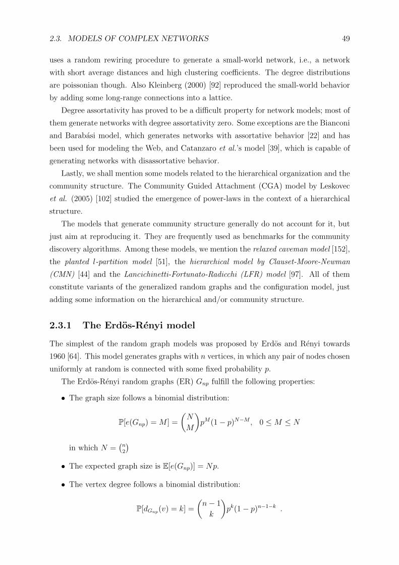
2.3. MODELS OF COMPLEX NETWORKS 49
uses a random rewiring procedure to generate a small-world network, i.e., a network
with short average distances and high clustering coefficients. The degree distributions
are poissonian though. Also Kleinberg (2000) [92] reproduced the small-world behavior
by adding some long-range connections into a lattice.
Degree assortativity has proved to be a difficult property for network models; most of
them generate networks with degree assortativity zero. Some exceptions are the Bianconi
and Barabasi model, which generates networks with assortative behavior [22] and has
been used for modeling the Web, and Catanzaro et al.’s model [39], which is capable of
generating networks with disassortative behavior.
Lastly, we shall mention some models related to the hierarchical organization and the
community structure. The Community Guided Attachment (CGA) model by Leskovec
et al. (2005) [102] studied the emergence of power-laws in the context of a hierarchical
structure.
The models that generate community structure generally do not account for it, but
just aim at reproducing it. They are frequently used as benchmarks for the community
discovery algorithms. Among these models, we mention the relaxed caveman model [152],
the planted l-partition model [51], the hierarchical model by Clauset-Moore-Newman
(CMN) [44] and the Lancichinetti-Fortunato-Radicchi (LFR) model [97]. All of them
constitute variants of the generalized random graphs and the configuration model, just
adding some information on the hierarchical and/or community structure.
2.3.1 The Erdos-Renyi model
The simplest of the random graph models was proposed by Erdos and Renyi towards
1960 [64]. This model generates graphs with n vertices, in which any pair of nodes chosen
uniformly at random is connected with some fixed probability p.
The Erdos-Renyi random graphs (ER) Gnp fulfill the following properties:
• The graph size follows a binomial distribution:
P[e(Gnp) = M ] =
(N
M
)pM(1− p)N−M , 0 ≤M ≤ N
in which N =(n2
)• The expected graph size is E[e(Gnp)] = Np.
• The vertex degree follows a binomial distribution:
P[dGnp(v) = k] =
(n− 1
k
)pk(1− p)n−1−k .

50 CHAPTER 2. COMBINATORIAL MODELS OF COMPLEX SYSTEMS
• The expected degree is E[dGnp(v)] = (n− 1)p.
• The expected clustering coefficient for a vertex is E[ccGnp(v)] = p.
• Degree assortativity is asymptotic to 0 with n→∞.
• The diameter is asymptotic to lnn/ ln(pn) with n→∞ [42].
• The graph is connected with high probability.
• Edge-connectivity is asymptotic to (n− 1)p with n→∞.
Figure 2.11: Erdos-Renyi model. Visualization. Instance of an Erdos-Renyi randomgraph with 100 vertices and expected degree 5.
It is usual to study the behavior of the Erdos-Renyi random graphs as n→∞ while
keeping np constant, so as to conserve the expected vertex degree. Under this restriction,
as n→∞ it holds that:
• Degree distribution converges to a Poisson distribution with mean np.
• The vertex clustering coefficient and the global clustering coefficient are asymptotic
to 0.
• The graph is disconnected (the diameter tends to infinity).

2.3. MODELS OF COMPLEX NETWORKS 51
The Erdos-Renyi graphs are not appropriate for modeling complex networks, as they
have degree distributions with an exponential fall off (instead of a heavy tail) and short
clustering coefficients. Also, the absence of correlations produces a degree assortativity
close to zero.
Degree
Re
lative
Fre
qu
en
cy
1 3 5 7 9 11 13 15
00
.05
0.1
0.1
5
0 5 10 15
05
10
15
k
k’
knn(k)
Figure 2.12: Erdos-Renyi model. Instance of a random graph generated with an Erdos-Renyi model, with p = 0.00025 and n = 20000. Its average degree is d = 5.00, and itsmaximum degree is dmax = 16. (Left) Relative frequency of the vertex degrees, comparedwith a binomial distribution with the same expected degree. (Right) Correlation betweenadjacent vertex degrees. Dots represent the mean of the neighbors’ degrees, knn, as afunction of vertex degree. The slope of the regression line (which equals the degreeassortativity) is null. The global clustering coefficient is also zero.
2.3.2 Internet models
Next, we shall describe 3 models used for studying the Internet topology: Waxman’s
model, the Barabasi-Albert model and the FKP model.
2.3.2.1 Waxman’s model
After performing some observations on the Internet, Waxman suggested two hypothesis
regarding how the routers connect among them. According to Waxman’s paper from
1988 [154]:
1. Routers in the Internet are geographically distributed, and this distribution affects
the way in which they are connected.

52 CHAPTER 2. COMBINATORIAL MODELS OF COMPLEX SYSTEMS
2. As a consequence of a resource optimization process, connections are more likely
to occur between close routers than between distant ones.
Considering these two ideas, Waxman introduced a change in the Erdos-Renyi model
in order to make the connection probability distance-dependent. In Waxman’s model,
n vertices are randomly positioned in a square of side L. Then, each pair of vertices
(vi, vj) is connected with a probability pij which is exponential on the euclidean distance
between them, which we denote as d(vi, vj):
pij = βe−d(vi,vj)
αL , 0 < α, β ≤ 1 .
The β constant determines the expected degree of the model. The α constant regulates
the exponential fall off, and thus it determines the probability of establishing long-
distance connections between the vertices.
This model was the first one that intended to reproduce the Internet topology.
Nonetheless, it shares many of the limitations of its predecesor: the vertex degree distri-
butions still have an exponential fall off.
−1.0 −0.5 0.0 0.5 1.0
−1.0
−0.5
0.0
0.5
1.0
Figure 2.13: Waxman’s model. Visualization. Instance of a graph generated with Wax-man’s model, with α = 0.22 and β = 0.30, with n = 200 vertices and 529 edges. Theaverage degree is d = 5.29.

2.3. MODELS OF COMPLEX NETWORKS 53
Degree
Re
lative
Fre
qu
en
cy
1 3 5 7 9 11 13
00
.05
0.1
0.1
50
.2
0 2 4 6 8 10 12 14
02
46
81
01
21
4
k
k’
knn(k)
Figure 2.14: Waxman’s model. Instance of a graph generated with Waxman’s model,with α = 0.15 and β = 0.0008, containing n = 20000 vertices. The average degree isd = 6 and the maximum degree is dmax = 14. The global clustering coefficient is almostzero. The degree assortativity is 0.043. The average distance is 8.59, and the diameteris 19.
2.3.2.2 The Barabasi-Albert model
When Faloutsos et al. showed that the degree distributions in the Internet followed
a power-law [66], many models tried not only to reproduce this property, but also to
explain it. The first of them was the model by Barabasi and Albert (BA) (1999) [14].
In their work, Barabasi and Albert discovered the presence of power-laws in the
degree distributions of different complex networks, as the Web, a cocitation network,
and the power distribution network of the United States. They also showed that the
previous models (like the Erdos-Renyi and the Watts-Strogatz models) could not capture
this scale-free property of the degree distributions. Then, they proposed a new model
in order to obtain power-laws. This model was based upon two hypotheses: network
growth and the preferential attachment mechanism.
Growth. The first of the two hypotheses was related to the dynamical evolution of
networks. As time evolves, networks incorporate new vertices. The authors pointed out
that the previous models failed partly because they considered a fixed initial number of
vertices.
Preferential attachment. According to this hypothesis, when a new vertex ap-
pears, it prefers to connect towards other well-connected vertices (i.e., high-degree ones).

54 CHAPTER 2. COMBINATORIAL MODELS OF COMPLEX SYSTEMS
Barabasi and Albert used the Web as example: The Web contains relatively few famous
sites, and when new pages appear they usually contain links towards them. With this
mechanism the authors applied an idea which was in fact present since many years. We
mention for example Price’s work on scientific collaborations from 1976 [128], and the
social aphorism known as the-rich-get-richer.
Under the BA (Barabasi-Albert) model, a network initially contains m0 vertices con-
nected among them. We shall call this initial graph as G0. This graph evolves through
discrete time, and one vertex is added in each time step. At time t, given the graph
Gt−1 = (Vt−1, Et−1), a vertex vt is added in order to obtain a graph Gt. This vertex
connects to a number m ≤ m0 of vertices in Vt−1, which are chosen with a probability
distribution in which the probability of choosing vj is proportional to its degree:
p(v(j)) =dGt−1(j)∑
k≤t−1 dGt−1(vk), j ≤ t− 1 .
From this simple rule, and after some time, the degree distribution arrives at a sta-
tionary state in which it is scale-free. This behavior was empirically showed by Barabasi
and Albert and later proved by mean-field approaches based on rate equations [15, 93].
The BA model description in [14] is somewhat inaccurate, as observed by Bollobas
et al. [30]. In particular, the layout of the initial m0 vertices (i.e., their connections)
is not described in the model. In each step, when choosing the m connections, the
joint distribution of them is not specified, but only the marginal distribution of each
connection. Nonetheless, the general scale-free properties of the model do not seem to
depend upon these choices.
The network graphs generated under the BA model present the following properties
in the stationary state (n→∞):
• The mean degree d is asymptotic to 2m.
• The global clustering coefficient is asymptotic to m−18n(G)
ln(n(G))2 [28].
• The degree distribution converges to a power-law with exponent α = 3.
• The average distances are those of small-world networks (i.e., they are shorter than
ln(n(G)) with high probability) [49].
• The diameter is asymptotic to ln(n(G))ln ln(n(G))
for m ≥ 2 [29].
• The degree assortativity is asymptotic to 0.

2.3. MODELS OF COMPLEX NETWORKS 55
• The graph is connected.
Even though the original BA model tends to generate power-laws with exponent α =
3, a simple adjustment makes it possible to get power-laws with exponents α ≥ 2 [60].
In conclusion, this model reproduces the power-laws which are present in many com-
plex networks, but it does not wholly reproduce the small-world phenomenon: the net-
works generated under the BA model have small diameters but their clustering coeffi-
cients are too short.
2.3.2.3 The FKP model
The model by Fabrikant et al. (FKP) [65] stands out for having applied the Highly
Optimized Tolerance (HOT) mechanism proposed by Carlson and Doyle [36] in 1999 for
obtaining power-laws in the degree distribution. Let us recall that the HOT mechanism
suggested that power-laws in complex systems emerged as the result of resource opti-
mization. Following this idea, Fabrikant et al. proposed an evolutive model in which the
vertices are added dynamically and are randomly positioned in space (in a similar way
as in Waxman’s model). But the connections between the vertices are not determined
by a probability distribution. When the i-th vertex is added, just a single connection is
established, which is determined as the one that minimizes a cost function, Ψ(vi, vj):
Ψ(vi, vj) = α(n(G))d(vi, vj) + φ(vj), j ≤ i− 1 ,
in which:
• α(n(G)) is a function of the final number of vertices. Its role is to determine the
relative weight of each of the two terms in the formula.
• d(vi, vj) represents the euclidean distance between vi and vj.
• φ(vj) is the inverse of some centrality measure on the vertices. E.g., it might be
the inverse of the betweenness, or the closeness.
A connection is established between vi and the vertex that minimizes this cost.
The minimization of the functional Ψ(vi, vj) defines a trade-off between two aspects:
the economic cost of establishing the link (measured under the euclidean distance) and its
utility, measured as the vertex centrality in the network. The FKP model successfully
reproduces a power-law in the degree distribution, but it generates graphs with core
number 1 (their maximal non-empty k-core is the 1-core), which have a tree structure
and whose global clustering coefficient is zero. A method extension proposed by Alvarez-
Hamelin and Schabanel solves this last limitation [9].

56 CHAPTER 2. COMBINATORIAL MODELS OF COMPLEX SYSTEMS
k
p(k
)
100
100.5
101
101.5
102
102.51
0−
61
0−
51
0−
41
0−
31
0−
21
0−
11
00
Clustering coefficient
Re
lative
Fre
qu
en
cy
0.025 0.225 0.425 0.6251e
−0
50
.00
10
.1
0 50 100 150 200
05
10
15
20
k
k’
knn(k)
Figure 2.15: Barabasi-Albert model. Instance of a graph generated with a Barabasi-Albert model (BA) with m = 3 and n = 20000 vertices. The average degree is d = 6and the maximum degree is dmax = 222. Upwards, to the left, a visualization of thegraph after adding the first 200 vertices. To the right, a log-histogram of the degreedistribution of the vertices, adjusted to a power-law with exponent α = 3.10, by themax-likelihood method. Downwards to the right, a histogram of the vertex clusteringcoefficients, grouped with a linear binning. To the left, the correlation between adjacentvertex degrees. The dots represent the mean value of the neighbors’ degrees, knn, as afunction of vertex degree. The slope of the regression line (i.e., the assortativity of thegraph) is −0.004. The clustering coefficient is almost zero. The average distance is 4.71and the diameter is 7.

2.3. MODELS OF COMPLEX NETWORKS 57
−1.0 −0.5 0.0 0.5 1.0
−1
.0−
0.5
0.0
0.5
1.0
k
p(k
)
100
100.5
101
101.5
102
102.51
0−
61
0−
51
0−
41
0−
31
0−
21
0−
11
00
10
1Figure 2.16: FKP model. Instance of a graph generated under the FKP model, withα = 25 and n = 20000 vertices. Closeness has been used as centrality measure. Themean degree is d = 2, the maximum degree is dmax = 229 and the global clusteringcoefficient is zero. The average distance is 6.70 and the diameter is 12. To the left, agraph visualization after connecting the first 200 vertices, in which the vertex positionrepresents its geographical location. To the right, a log-histogram of the degree distribu-tion, adjusted by a power-law for k ≥ 2, with exponent α = 1.67, by the max-likelihoodmethod.
The network graphs generated under the FKP model have the following properties:
• For 4 ≤ α(n(G)) <√n(G) the degre distribution is asymptotic to a power-law
with exponent bigger than 1 as n → ∞ (the authors prove this when using the
graph distance between the vertices and a fixed vertex as centrality measure).
• The global clustering coefficient is zero.
• The mean degree is asymptotic to 2.
2.3.3 Generalizations of the Erdos-Renyi model
The original Erdos-Renyi model generates network graphs with poissonian degree distri-
butions, in which vertex degrees have scarse dispersion. These graphs are usually called
as homogeneous. Some proposals were made for adapting the ER model in order to
obtain heterogeneous graphs and, in particular, graphs with scale-free distributions. We

58 CHAPTER 2. COMBINATORIAL MODELS OF COMPLEX SYSTEMS
shall now describe two of them: the configuration model and the random graph with
specified expected degrees.
In the configuration model [21] a specific degree sequence is guaranteed. According
to the prescribed degrees d(vi), each vertex i is connected to a number of d(vi) stubs
(which can be thought as edge endpoints). From the set of 2e(G) stubs, two of them are
randomly chosen and connected19. The process is repeated (without reposition of the
stubs) until no stubs remain. Necessarily, when the process ends, each vertex will have
the specified degree for it. As one of its properties, this model obtains an equiprobable
sample from the set of all non-isomorphic graphs with some fixed degree distribution.
In the random graph model with specified expected degrees [43], each pair of vertices
vi and vj is connected with a probability pij =DiDj∑iDi
, so that the expected degree for
some vertex i is E[d(vi)] = Di.
Figure 2.17: Configuration model and random graph model with specified expected degrees.In the configuration model (Left) each vertex connects to a number of stubs equal to itsprescribed degree. The stubs are chosen by pairs, in a random fashion, and they areconnected until no stub remains. In the random graphs with specified expected degrees(Right) the probability of connecting two vertices vi and vj is pij =
DiDj∑iDi
, where Di is
the expected degree for vertex i.
In both models, the introduction of scale-free distributions also reproduces part of
the small-world phenomenon: the expected average distance, for values of α between 2
and 3, tends asymptotically to 2log(log(n(G)))log(α−2)−1 as n→∞, and the diameter is in the order
of n(G). But none of them reproduces the high clustering coefficients of small-world
networks [133, 43].
19Each stub is chosen with uniform distribution from among the remaining ones. The configurationmodel may generate graphs with loops and multiedges.

2.3. MODELS OF COMPLEX NETWORKS 59
2.3.4 Models of Social Networks
We shall now describe the characteristics of the Watts-Strogatz model. This model was
the first to fully reproduce the small-world behavior. We shall also introduce some of
the models used to generate community structure: the planted l-partition model and the
Lancichinetti-Fortunato-Radicchi (LFR) model.
2.3.4.1 The Watts-Strogatz model
Many complex networks (specially the social ones) present small-world behavior. This
behavior can be described as the presence of small average distances between vertices
and high clustering coefficients.
Watts and Strogatz tried to reproduce this problem in a graph model with fixed
average degree [153]. In the Erdos-Renyi model we showed that it was not possible. If we
kept the np product fixed, when n was large enough we got a disconnected network an and
clustering coefficient tending to zero. The authors compare this situation against that of
lattices, in which the clustering coefficient is high but the average distance may be very
high too. Looking for a half-way point between these two cases, they proposed a model
whose initial structure is a ring in which vertices only connect with all their neighbors at
distance at most k (in this way, a high clustering coefficient is obtained) and a rewiring
procedure is performed in which the edges uv are removed with some probability p,
and new edges uw are set with a randomly chosen vertex w. This rewiring procedure
does not change the total number of edges in the graph, and thus the average degree is
conserved. Increasing the probability p shortens the average distance but also the global
clustering coefficient. But, for a wide range of values of p (between n−1 p 1) the
model obtains graphs with small average distances and a high clustering coefficient.
The random graphs obtained with the Watts-Strogatz model have the following prop-
erties [17]:
• The size of the graph is kn.
• For n→∞ and p→ 1, the degree distribution converges to a Poisson distribution
with mean k.
• In the region n−1 p 1 the expected clustering coefficient is 3(k−1)2(2k−1)
.
• In the region n−1 p 1 the expected distance between vertices is lnn/ ln k.
Although the degree distribution of the graphs generated under the Watts-Strogatz
model is still poissonian, its importance lies in being the first to fully reproduce the
small-world behavior.
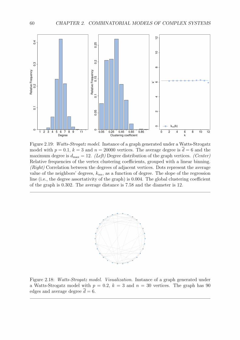
60 CHAPTER 2. COMBINATORIAL MODELS OF COMPLEX SYSTEMS
Degree
Rela
tive
Fre
quency
1 2 3 4 5 6 7 8 9 11
00.1
0.2
0.3
0.4
Clustering coefficient
Rela
tive
Fre
quency
0.05 0.25 0.45 0.65 0.85
00.0
50.1
0.1
50.2
0.2
5
0 2 4 6 8 10 12
02
46
810
12
k
k’
knn(k)
Figure 2.19: Watts-Strogatz model. Instance of a graph generated under a Watts-Strogatzmodel with p = 0.1, k = 3 and n = 20000 vertices. The average degree is d = 6 and themaximum degree is dmax = 12. (Left) Degree distribution of the graph vertices. (Center)Relative frequencies of the vertex clustering coefficients, grouped with a linear binning.(Right) Correlation between the degrees of adjacent vertices. Dots represent the averagevalue of the neighbors’ degrees, knn, as a function of degree. The slope of the regressionline (i.e., the degree assortativity of the graph) is 0.004. The global clustering coefficientof the graph is 0.302. The average distance is 7.58 and the diameter is 12.
Figure 2.18: Watts-Strogatz model. Visualization. Instance of a graph generated undera Watts-Strogatz model with p = 0.2, k = 3 and n = 30 vertices. The graph has 90edges and average degree d = 6.

2.3. MODELS OF COMPLEX NETWORKS 61
2.3.4.2 The planted l-partition model
The planted l-partition model was proposed by Condon and Karp in 2001 [51] in the
context of data mining, as a benchmark for the clustering task.
This model builds a graph Gn with n vertices grouped into l communities, all of them
equally-sized, which form a partition of the vertex set. After this initial assignment, each
pair of vertices (u, v) is considered, and they are connected with some probability pi if
they belong to the same community, and with a different probability po < pi if they
belong to different communities. In this way, vertices tend to be more connected inside
their communities than towards the outside.
The graphs obtained under this model have homogeneous vertex degrees, with ex-
pected degree E[d] = pi(nl− 1)
+ pon(l−1)
land scarse dispersion.
The Girvan-Newman (GN) benchmark [76], with n = 128 and l = 4, is a particular
case of the planted l-partition model, in which the probabilities pi and po are chosen so
that the expected degree of the vertices is E[d(v)] = 16, which determines the relation
31pi + 96po = 16, po < pi .
2.3.4.3 The LFR model
This model proposed by Lancichinetti, Fortunato and Radicchi in 2008 [97] generates
graphs with heterogeneous distributions both in the vertex degrees as in the community
sizes. It is adjusted by a series of parameters20:
• n, the size of the graph, n(G).
• γ, the exponent of the power-law for the vertex degree distribution.
• d, the average degree for the power-law.
• dmax, the maximum vertex degree.
• β, the exponent of the power-law for the community size distribution21.
• smin, the minimum size of a community.
• smax, the maximum size of a community.
20We do not describe here the two parameters related to the definition of overlappings betweencommunities.
21The authors define the community size as the sum of the vertex degrees.

62 CHAPTER 2. COMBINATORIAL MODELS OF COMPLEX SYSTEMS
5
3
11
1915
17
01
7
213
6
4
8
1612
1814
925
36
24
39
27
29
303335
2622
20
23
31
28
38
34
32
4452
46 5359
49
404142
45
43
50
54
47
5658
92
9580
83
81
86
85
84
88
87
89
97
91
98
94
96
6864
65
66
70 61
62
63
69
717672
77
74
79
102
112105
107
101106
117
100
103 109
116
110
119
0
1
2
3
4
5
6
Figure 2.20: Planted l-partition model. Instance of a graph generated under the plantedl-partition model, with 120 vertices organized into 6 communities. The connection prob-abilities inside and outside the communities are 0.4 and 0.02 respectively. The visual-ization was generated with the LaNet-vi software, using the k-dense decomposition ofthe graph. The scale on the right represents the dense index of the vertices. Verticesin the same community have consecutive numbers, so that a vertex vi belongs to thecommunity d i
20e.
• µ, to so-called mixing parameter, which specifies the ratio of the external connec-
tions (towards other communities) of the vertices to their degree.
• C, a desired value for the global clustering coefficient.
The graph is built by performing the following steps:
1. Each vertex is assigned a degree which is taken from a power-law with a cut-off
(d ≤ dmax), with exponent γ and expected degree d.
2. The connections are made in the same way as in the configuration model.
3. The community sizes are assigned from a power-law with a cut-off (s ≤ smax), with
exponent β and minimum size smin.

2.3. MODELS OF COMPLEX NETWORKS 63
4. Each vertex is assigned a community at random, under the restriction that after
the inclusion of the vertex, the community should not exceed its assigned size. A
successive refinement procedure is performed until all vertices are assigned to a
community.
5. A rewiring procedure is made in order to adjust the µ values of the vertices to the
specified µ.
6. Finally, a second rewiring is performed in order to adjust the clustering coefficient
to its desired value.

64 CHAPTER 2. COMBINATORIAL MODELS OF COMPLEX SYSTEMS
Degree
Re
lative
Fre
qu
en
cy
1 5 9 14 20 26 32 38 44 50
00
.05
0.1
0.1
50
.2
Clustering coefficient
Re
lative
Fre
qu
en
cy
0.05 0.25 0.45 0.65 0.85
00
.05
0.1
0.1
50
.20
.25
0 10 20 30 40 50
01
02
03
04
0
k
k’
knn(k)
Figure 2.21: LFR model. Instance of a graph generated under the Lancichinetti-Fortunato-Radicchi (LFR) model, with the following parameters: n = 256, d =10, dmax = 50, γ = 2.0, β = 1.0, µ = 0.2, smin = 10, smax = 50, C = 0.4. This instancehas an average degree of 10.84, an average µ of 0.199 and a clustering coefficient of 0.41.The visualization was produced with the Gephi software. The vertex colors representthe communities they belong to, and their sizes are proportional to their degree. Belowwe show the degree distribution, a histogram of the clustering coefficients of the vertices,and the knn as a function of vertex degree.

Chapter 3
Discovering Communities in Social
Networks
Community structure arises from the organization of the members of a network into
groups, which we call communities. This organization is typical of many complex net-
works, especially the following ones:
• Social networks. The discovery of community structure makes it possible to study
relations between people, like friendship networks, workgroups and families. The
Internet has reduced the geographical barriers and impulsed the constitution of
virtual communities, in which people interact according to their cultural, political
or ideological affinity. The fact that these communities are founded on the informa-
tion technologies has important consequences. On one side, it offers large volumes
of data for scientific analysis, and it requires efficient processing methods. On the
other side is has a potential economical value: the information on people’s virtual
life helps companies discover their clients and offer their own services efficiently.
But the potential of information technology has also led to serious discussions on
information security and privacy in the virtual world.
• Scientific collaboration networks. Scientists cooperate and work in communities ac-
cording to their research areas. Some of these areas are prone to extense collabora-
tions between scientists. Other areas are quite close instead, and their communities
are smaller [111].
• The Web. Web sites are organized into communities around some topics. These
communities arise spontaneously from the established hyperlinks [68].
• Metabolic networks. This type of biological network represents compounds (i.e.
metabolites) evolution along chemical processes or cycles. In each process, a series
65

66 CHAPTER 3. DISCOVERING COMMUNITIES IN SOCIAL NETWORKS
of reactions takes place in which some metabolites react and produce some others.
The network formed by all the metabolites has a community structure in which
metabolites are organized into modules. Each module is correlated with one or
more cycles or processes [86].
• Networks of protein interactions. In live organisms, proteins interact inside cells in
order to take part in some vital processes. Each of these processes performs some
important function for the organism. Discovering community structure in protein
networks is a powerful tool for inferring functionality from structure [41].
• Trophic networks. Discovering communities in ecosystems helps studying trophic
relations among the species. The notion of community is here related to the concept
of ecological compartment [94].
In general terms, the potential of community discovery is related to its capacity for
inferring relations between the network members, predicting their behavior or future
decisions, and understanding the way in which communities arise and evolve.
This chapter presents the following structure: in the first section, we discuss the
notion of community and some of its interpretations; in 3.2 we briefly describe the
state of the art in community discovery; then we stress the need for defining appropriate
comparison metrics. In sections 3.4 and 3.5 we present our contribution to the community
discovery problem in complex networks. This contribution is contained in our articles [33,
20].
3.1 Introduction to the notion of community
An important precedent for community study in complex networks is provided by the
data mining problem known as data clustering. In the data clustering problem, the
elements of a set are to be grouped into clusters according to their properties (which are
usually modeled as coordinates in an n-dimensional space. In this problem, a notion of
distance between elements is usually defined, and the assignment of elements intends to
produce compact clusters, i.e., with small distances between intra-cluster elements.
In the community discovery problem, instead, two main differences arise:
1. The existence of communities is uncertain, so that the community discovery method
is expected to determine if they exist, in addition to how many and which they
are.
2. Vertex assignment into a community in mainly determined by the connections they
have. There is no need to define any distance.

3.1. INTRODUCTION TO THE NOTION OF COMMUNITY 67
However, some community discovery methods introduce a distance notion and even
apply traditional data clustering methods, especially those of hierarchical clustering.
Another important precedent is set by the studies of cohesion in social groups. Group
cohesion (i.e., strength of its links) may determine the production of uniform opinion or
influence over its members. From the 40es on, sociologists have introduced concepts as
the cliques [106], the n-cliques [1], the k-plexes [142], the n-clans [109], the n-clubs [109]
and the LS sets [98] for studying group cohesion (see Figure 3.1).
In the area of complex networks, the notion of community began to take shape with
the works by Flake et al. (2000) [68] and Newman and Girvan (2001) [111]:
• Flake et al. [68] proposed the notion of web community as that of a set of vertices
C ⊂ V (G) in which each vertex has more neighbors inside the set than outside of
it. This can be expressed (using the notation introduced in Table 3.2) as:
∀v ∈ C : dinC (v) > doutC (v) .
• Newman analyzed in [111] the concept of community in the context of a scientific
collaboration network. In this network, he observed that the existence of commu-
nities was related to the observation of high clustering coefficients: two scientists,
who had each of them collaborated with a third one, may also have worked together
with high probability.
Since then, the interest on studying community structure has increased year after
year.

68 CHAPTER 3. DISCOVERING COMMUNITIES IN SOCIAL NETWORKS
Structure Definition Example
clique of order kmaximally complete subgraph with k ver-tices.
n-cliquemaximal set of vertices such that all of themlie at a distance at most n. Example: 2-clique.
k-plexmaximal subgraph with n vertices in whicheach vertex is connected to at least n − kothers. Example: 3-plex.
n-clann-clique whose induced subgraph has diame-ter at most n. Example: 2-clan.
n-cluba maximal subgraph of diameter at most n.Example: 2-club.
LS setset of vertices such that each vertex has moreconnections to others in the same set than toexternal vertices.
Table 3.1: Some cohesive structures used for studying social groups.

3.2. COMMUNITY DISCOVERY METHODS. STATE OF THE ART 69
3.2 Community discovery methods. State of the Art
We shall now describe the evolution of community discovery and some of its best-known
methods. We shall classify the methods into local and global ones. Global methods
are those in which the communities arise from a problem defined over the whole graph
(e.g., a functional minimization). Local methods are those in which the communities are
based on the local structure and are not affected by the structure of other areas of the
graph. We shall see that community study evolved from global into local methods, and
nowadays the later are preferred. For a deeper comprehension of the state of the art we
suggest consulting the exhaustive survey by Fortunato [70].
We did already mention the seminal work by Newman on scientific collaboration
networks. One year later, Newman developed a divisive hierarchical clustering method
for community discovery based on the edge-betweenness (2002) [76] (see our Subsec-
tion 2.1.3.1). This method is based on the idea that those edges which connect vertices
in the same communities should have a smaller edge-betweenness as compared to that
of edges connecting vertices in different communities. This occurs because the latter
are more probable to take part into minimum paths between those vertices. Thus, the
proposed algorithm computes the edge-betweenness for every edge, and removes them
sequentially, beginning by those of higher edge-betweenness. As the graph disconnects, a
dendrogram is built whose branches represent the connected components. The algorithm
updates the edge-betweenness after each edge removal; this makes it computationally ex-
pensive.
Radicchi et al. (2004) [129] suggested a variation of Newman’s algorithm in which the
edge-betweenness is replaced by the edge-clustering coefficient, which they introduced. In
the same work, they noticed the need for counting on a non-operational definition of com-
munity (i.e., one which were not based just in the result of some algorithm or method).
This would make it possible to evaluate and compare different detection methods, and
even to decide if the structures they find are significant or not. Radicchi et al. suggest
two definitions of community:
1. Community in a strong sense. A set C ⊂ V (G) is a community in a strong sense
if:
∀v ∈ C : dinC (v) > doutC (v) .
2. Community in a weak sense. A set C ⊂ V (G) is a community in a weak sense if:
∑v∈C
dinC (v) >∑v∈C
doutC (v) .
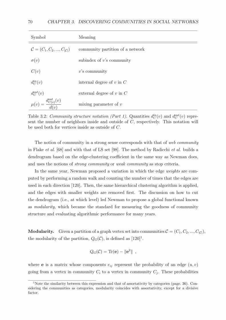
70 CHAPTER 3. DISCOVERING COMMUNITIES IN SOCIAL NETWORKS
Symbol Meaning
C = (C1, C2, ..., C|C|) community partition of a network
σ(v) subindex of v’s community
C(v) v’s community
dinC (v) internal degree of v in C
doutC (v) external degree of v in C
µ(v) =doutC(v)(v)
d(v)mixing parameter of v
Table 3.2: Community structure notation (Part 1). Quantities dinC (v) and doutC (v) repre-sent the number of neighbors inside and outside of C, respectively. This notation willbe used both for vertices inside as outside of C.
The notion of community in a strong sense corresponds with that of web community
in Flake et al. [68] and with that of LS set [98]. The method by Radicchi et al. builds a
dendrogram based on the edge-clustering coefficient in the same way as Newman does,
and uses the notions of strong community or weak community as stop criteria.
In the same year, Newman proposed a variation in which the edge weights are com-
puted by performing a random walk and counting the number of times that the edges are
used in each direction [120]. Then, the same hierarchical clustering algorithm is applied,
and the edges with smaller weights are removed first. The discussion on how to cut
the dendrogram (i.e., at which level) led Newman to propose a global functional known
as modularity, which became the standard for measuring the goodness of community
structure and evaluating algorithmic performance for many years.
Modularity. Given a partition of a graph vertex set into communities C = (C1, C2, ..., C|C|),
the modularity of the partition, QG(C), is defined as [120]1.
QG(C) = Tr(e)− ‖e2‖ ,
where e is a matrix whose components eij represent the probability of an edge (u, v)
going from a vertex in community Ci to a vertex in community Cj. These probabilities
1Note the similarity between this expression and that of assortativity by categories (page. 36). Con-sidering the communities as categories, modularity coincides with assortativity, except for a divisivefactor.

3.2. COMMUNITY DISCOVERY METHODS. STATE OF THE ART 71
can be computed as
eij =|(Ci, Cj)|
2e(G)=
∑(u,v)∈Ci×Cj 1u→ v
2e(G).
From here it follows [45]
QG(C) =1
2e(G)
∑(vi,vj)∈V (G)×V (G)
[Aij −
d(vi)d(vj)
2e(G)
]1σ(vi) = σ(vj) , (3.1)
where 1σ(vi) = σ(vj) equals 1 when vi and vj belong to the same community, and 0
otherwise.
The first term of modularity, which is determined by Tr(e), equals the ratio of inter-
nal edges (i.e., edges connecting vertices in the same communities) to the total number
of edges. The second term evaluates the expected ratio of internal edges under a random
graph model with the same vertices, expected degrees and assigned communities2. We
shall thus say that modularity measures the goodness of a community structure by com-
paring its ratio of internal edges to the expected ratio of internal edges if the connections
were made at random.
By assuming that the higher the modularity the better the community structure,
Newman suggested that the best community partition would be the one that maximizes
the Q value. Modularity maximization is a combinatorial optimization problem3 which is
computationally expensive. Brandes et al. proved that it is NP-complete [31]. However,
it can be approached by heuristic methods.
From being an quantitative measure of community structure, modularity turned
into a global functional to be optimized. From among the many modularity maxi-
mization methods, we recall: the greedy algorithm by Clauset-Newman-Moore (CNM,
2004) [45], that of Guimera et al. based on simulated annealing (2004) [85], the ex-
tremal optimization method by Duch and Arenas (2005) [63], the method by Danon et
al. (2006) [53], Newman’s method of spectral bisection [117], that of Wakita and Tsu-
rumi (2007) [151], the one by Blondel et al. (2008) [24] and the multilevel algorithm by
Noack and Rotta (2009) [121]. Some modularity extensions have also been proposed for
directed graphs [99] and weighted graphs [10].
The limitations found in modularity (which we discuss in Section 3.4), especially its
scaling limit, inspired the research on local methods of community detection. One of
2This null model is built according to the random graph model with specified expected degrees (seepage 58).
3It falls into the category of quadratic assignment problems.

72 CHAPTER 3. DISCOVERING COMMUNITIES IN SOCIAL NETWORKS
the first local methods was the Clique Percolation Method (CPM) proposed by Palla et
al. (2005) [123]. This method builds the communities through a percolation process of
cliques of order k. It does not find partitions but covers, in which communities may
overlap.
Raghavan et al. (2007) [130] proposed a local algorithm which finds a partition by
using a label propagation algorithm. First, the algorithm assigns each vertex a different
label. Then, through an iterative process, each vertex replaces its label by the most
frequent one among its neighbors4. The stop criterion consists on verifying that every
vertex has at least as many edges inside its community as outside of it5. Even though
the algorithm might be unstable (in fact, convergence is not guaranteed) in the complex
networks studied by them convergence is verified after a few iterations. In this method,
the idea is implicit that communities play an important role into diffusion processes.
This idea is also present in other percolation and spectral methods. Tibely and Kertesz
showed that Raghavan et al.’s process is equivalent to finding a local minimum of a Potts
model Hamiltonian [148].
In 2009 Lancichinetti et al. proposed a local method based in the concept of natural
community [96]. The natural community of a vertex is defined by construction, by
departing from the vertex and adding (and sometimes removing) vertices so as to increase
the community’s (fitness function), defined as: [96]
fL(C) =din(C)
(din(C) + dout(C))α, (3.2)
where din(C) and dout(C) represent the sum of the internal and external degrees of the
vertices in C (see this notation in Table 3.3).
The method by Lancichinetti et al. finds graph covers, as each vertex may belong
to more than one natural community. Besides, the fitness function offers a quantitative
measure of the community significance.
Many researchers have analyzed the community sizes of complex networks and have
found heavy-tailed distributions. This phenomenon had been observed in 2002 by
Guimera et al in the e-mail exchange network [87], by Gleiser and Danon in 2003 in
the jazz network [78] and by Newman in the scientific collaboration network [113] in
2003. In all these cases, the results were obtained by modularity maximization, and
they showed power-laws over a range of about 3 decades in the logarithmic scale, with
exponents between 1.5 and 2. The limited size of those networks did not make it possible
4If a tie occurs, the label is randomly chosen from among those with maximum frequency.5This criterion is similar to that of community in a strong sense by Radicchi, with a ≥ sign instead
of >.

3.3. COMPARISON METRICS 73
to observe the effects of the scaling limit of modularity, which becomes more evident for
larger networks. The local methods by Lancichinetti et al. [96] and Palla et al. [123],
reproduced the same phenomenon over a larger range of values. In conclusion, the ex-
istence of a resolution limit for modularity questions its capacity for finding community
structures with scale-free degree distributions in heterogeneous networks. In Section 3.5.7
we will use the benchmark by Lancichinetti-Fortunato-Radicchi [97] in order to show the
effects of the scaling limit of modularity in the degree distribution of the communities.
Lastly, among the global methods we mention InfoMAP, which is based on a novel
idea proposed by Rosvall and Bergstrom (2008) [138]. In their work, the authors sug-
gested that the best community structure is the one which minimizes the description
length, i.e., the amount of information in a joint encoding of the community structure
and the graph. In other words, if a community structure is optimal, it should be possible
to recover the whole graph from the community assignment to vertices, with very little
additional information. At the same time, the amount of information of the community
assignment should not be excessive. The authors have minimized this global functional
by different methods, as simulated annealing [138] and random walks [139].
The description length. In order to compute the description length of a partition Cwe need: (i) a graph encoding in which each community is assigned a code, and (ii) a set
of internal encodings, one for each community, which assign a code to each vertex inside a
community. The description length thus represents the average length of the description
of an infinite random graph using this set of encodings. It is computed in the stationary
state of the Markov process associated to the graph. The minimum description length,
L(C), is the minimum average length from among all the encodings, and corresponds to
the Shannon limit. Its formula, which is known as map equation, can be found in [137].
Here we only write it in terms of our measures mV and cE, for undirected graphs:
L(C) =
(∑C∈C
cE(C)
)log
(∑C∈C
cE(C)
)− 2
∑C∈C
cE(C) log(cE(C))−
−∑
v∈V (G)
mV (v) log(mV (v)) +∑C∈C
(cE(C) +mV (C)) log(cE(C) +mV (C))
3.3 Comparison metrics
As the notion of community does not have a unique definition but rather depends on the
context, we need to establish criteria for measuring the goodness of the different commu-
nity discovery methods. In principle, we distinguish two ways to evaluate performance:

74 CHAPTER 3. DISCOVERING COMMUNITIES IN SOCIAL NETWORKS
Quantity Notation Definition Equivalences
Size s(Ci) |Ci|
Degree d(Ci)∑
v∈Ci d(v) |Ci, V (G)|
Degree measure mV (Ci)d(Ci)
2e(G)
Internal degree din(Ci)∑
v∈Ci dinCi
(v) |(Ci, Ci)|
Internal degree measure mE(Ci)din(Ci)
2e(G)
|(Ci, Ci)|2e(G)
External degree dout(Ci)∑
v∈Ci doutCi
(v) |(Ci, V (G)\Ci)|
External degree measure cE(Ci)dout(Ci)
2e(G)
|(Ci, V (G)\Ci)|2e(G)
Cut measure mE(Ci × Cj)|(Ci, Cj)|
2e(G)
Mixing parameter µ(Ci)mV (Ci)−mE(Ci)
mV (Ci)
∑v∈Ci
µ(v) · d(v)
d(Ci)
Table 3.3: Community structure notation (Part 2).
• Quantifying goodness of community structure by some global functional. As an ex-
ample we shall mention modularity [45] and the minimum description length [138].
In these cases, we would rather say that the functional imposes its own definition
of community structure.
• In networks with a priori defined communities, we may compare both community
structures (the a priori structure and the obtained one) by using a comparison
metric. Again, two possibilities arise:
– Using real networks. In a few real networks community structure is known.
Some examples are the karate network, the dolphins networks and the college
football network.
– Using random graphs with community structure as benchmarks. We recall
the Girvan-Newman benchmark, which is a particular case of the planted
l-partition model (see page 61), and the Fortunato-Lancichinetti-Radicchi
benchmark (see page 61).
In this section we shall discuss the following comparison metrics in the context of
the community detection problem: the mutual information, the Jaccard index and the

3.3. COMPARISON METRICS 75
fraction of correctly classified vertices6.
Mutual information The mutual information is used in Information Theory for quan-
tifying the amount of information in common between two or more random variables. In
order to use it as a measure of comparison between community structures, we shall define
two random variables, X1 and X2, associated to the partitions C1 = (C11, C12, ..., C1n)
and C2 = (C21, C22, ..., C2m) of a graph G [54]. Let us consider a random process in which
a vertex from V (G) is picked at random, with uniform distribution, and the subindex of
its community in the first partition, σC1(v), is observed. We define the random variable
X1 as the subindex of this community, which ranges between 1 and n. The probability
distribution for X1 is:
P[X1 = i] = pi =|C1i|n(G)
,
with i = 1, 2, ..., n. The entropy of the partition C1 is defined as:
H(C1) = −n∑i=1
pi · log (pi) .
We define the second random variable X2 in a similar way, but considering now the
partition C2. Then we define the following joint distribution for X1, X2:
P[X1 = i,X2 = j] = pij =|C1i ∩ C2j|n(G)
,
with i = 1, 2, ..., n, j = 1, 2, ...,m. The joint entropy of C1 and C2 is defined as:
H(C1, C2) = −n∑i=1
m∑j=1
pij · log (pij) ,
and the mutual information between them is:
MI(C1, C2) = H(C1) +H(C2)−H(C1, C2) .
6The term metric is not used here in a rigorous sense. The formal definition of metric requiresfulfilling conditions as positivity, symmetry and the triangular inequality. In this sense: (i) the mutualinformation is a metric if normalized in a specific way, but not as we do here; (ii) the Jaccard index,JI(x, y), produces a metric if 1 − J(x, y) is considered. J(x, y) would rather be a similarity measure;(iii) the fraction of correctly classified vertices is not a metric, as symmetry does not hold.

76 CHAPTER 3. DISCOVERING COMMUNITIES IN SOCIAL NETWORKS
The normalized mutual information between C1 and C2 is: [54]
NMI(C1, C2) =2MI(C1, C2)
H(C1) +H(C2)=
= −2 ·
∑ni=1
∑mj=1 pij · log
(pijpi·pj
)∑n
i=1 pi · log (pi) +∑m
j=1 pj · log (pj). (3.3)
The normalized mutual information lies between 0 and 1, and it gives a sense of the
similarity between two partitions, in terms of the information about one of them that
underlies in the other. It reaches a value of 1 when both partitions are coincident7.
Jaccard index The Jaccard index computes the ratio of vertex pairs assigned to the
same community in both partitions C1 and C2, to the number of vertex pairs which belong
to the same community in either one or both partitions. We introduce the following
quantities:
• a11: Number of pairs (v, w) assigned to the same community in both C1 and C2.
• a01: Number of pairs (v, w) assigned to the same community just in C2.
• a10: Number of pairs (v, w) assigned to the same community just in C1.
• a00: Number of pairs (v, w) assigned to different communities both in C1 as in C2.
This index is defined as:
JI(C1, C2) =a11
a11 + a01 + a10
.
We observe that a11, a01y a10 can be computed as:
a11 =∑C1i∈C1
∑C2j∈C2
|C1i ∩ C2j|(|C1i ∩ C2j|+ 1)
2,
a10 =∑C1i∈C1
|C1i|(|C1i|+ 1)
2− a11 ,
a01 =∑C2j∈C2
|C2j|(|C2j|+ 1)
2− a11 ,
7For a deeper analysis on the properties of the entropy and the mutual information in the contextof Information Theory, we suggest consulting the book by Cover and Thomas [52].
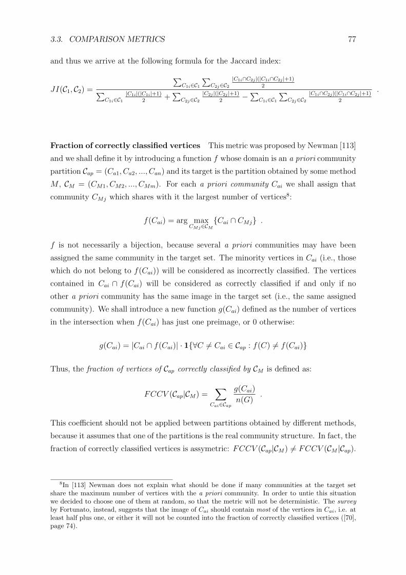
3.3. COMPARISON METRICS 77
and thus we arrive at the following formula for the Jaccard index:
JI(C1, C2) =
∑C1i∈C1
∑C2j∈C2
|C1i∩C2j |(|C1i∩C2j |+1)
2∑C1i∈C1
|C1i|(|C1i|+1)2
+∑
C2j∈C2|C2j |(|C2j |+1)
2−∑
C1i∈C1∑
C2j∈C2|C1i∩C2j |(|C1i∩C2j |+1)
2
.
Fraction of correctly classified vertices This metric was proposed by Newman [113]
and we shall define it by introducing a function f whose domain is an a priori community
partition Cap = (Ca1, Ca2, ..., Can) and its target is the partition obtained by some method
M , CM = (CM1, CM2, ..., CMm). For each a priori community Cai we shall assign that
community CMj which shares with it the largest number of vertices8:
f(Cai) = arg maxCMj∈CM
Cai ∩ CMj .
f is not necessarily a bijection, because several a priori communities may have been
assigned the same community in the target set. The minority vertices in Cai (i.e., those
which do not belong to f(Cai)) will be considered as incorrectly classified. The vertices
contained in Cai ∩ f(Cai) will be considered as correctly classified if and only if no
other a priori community has the same image in the target set (i.e., the same assigned
community). We shall introduce a new function g(Cai) defined as the number of vertices
in the intersection when f(Cai) has just one preimage, or 0 otherwise:
g(Cai) = |Cai ∩ f(Cai)| · 1∀C 6= Cai ∈ Cap : f(C) 6= f(Cai)
Thus, the fraction of vertices of Cap correctly classified by CM is defined as:
FCCV (Cap|CM) =∑
Cai∈Cap
g(Cai)
n(G).
This coefficient should not be applied between partitions obtained by different methods,
because it assumes that one of the partitions is the real community structure. In fact, the
fraction of correctly classified vertices is assymetric: FCCV (Cap|CM) 6= FCCV (CM |Cap).
8In [113] Newman does not explain what should be done if many communities at the target setshare the maximum number of vertices with the a priori community. In order to untie this situationwe decided to choose one of them at random, so that the metric will not be deterministic. The surveyby Fortunato, instead, suggests that the image of Cai should contain most of the vertices in Cai, i.e. atleast half plus one, or either it will not be counted into the fraction of correctly classified vertices ([70],page 74).

78 CHAPTER 3. DISCOVERING COMMUNITIES IN SOCIAL NETWORKS
3.4 Analysis of the Q functional (modularity)
Since its original expression, contained in Equation (3.1), the modularity has had several
interpretations. Here we present two of them, and introduce our own interpretation as
a signed measure, from which many of its properties will be deduced.
Interpretation as a quadratic assignment problem Smith and White (2005) [146]
restated the problem of modularity maximization as a quadratic assignment one. Given
a partition C, we define a vector xC of N elements for each community C ∈ C. This
vector will be assigned a value of 1 in its i-th position if and only if the vertex vi is
assigned to community C in the partition, and 0 otherwise. We may now rewrite the
modularity as:
QG(C) = −∑C∈C
xCTLQxC ,
where the matrix LQ has the following components:
lij =d2(vi)
4e2(G)− Aij
2e(G).
If all the vectors xC are joined into an assignment matrix X whose components xic
represent the assignment of community Cc to the vertex i, then we get to the following
expression:
QG(C) = −Tr(XTLQX) .
Modularity maximization has been thus restated as the problem of minizing the trace of
XTLQX, subject to the restriction that X is an assignment matrix, i.e., that XTX is a
diagonal matrix with discrete values 0, 1 and its trace is n(G).
This translation into a quadratic assignment problem leads to the use of spectral
decomposition methods, which compute the components of the main eigenvectors of
LQ. As the eigenvectors components are not discrete but continuous, usually some data
clustering algorithm as the k-means has to be applied in order to extract the communities.
Figure 3.1 illustrates this approach with the football network.
In 2006 Newman suggested using a similar approximation for the particular case of
graph bijection (i.e., a partition into 2 communities) computing the graph laplacian [117].
Interpretation as a Potts spin-glass model [132]. Reichardt and Bornholdt showed
that modularity is proportional to the Hamiltonian of a Potts model in which the spin
values σ(vi) of the vertices represent the subindexes of their communities in a partition

3.4. ANALYSIS OF THE Q FUNCTIONAL (MODULARITY) 79
−0.15 −0.05 0.05 0.10
−0.1
5−
0.0
50.0
50.1
5
Coordinates of the 1st eigenvector
Coord
inate
s o
f th
e 2
nd e
igenve
cto
r
−0.15 −0.05 0.05 0.10
−0.2
−0.1
0.0
0.1
0.2
Coordinates of the 1st eigenvector
Coord
inate
s o
f th
e 3
rd e
igenve
cto
rFigure 3.1: Spectral methods in community discovery. Football network. Here we applythe spectral decomposition of the matrix LQ to the football network. The vertex coor-dinates will be determined by the main eigenvectors of the matrix. In these figures weonly show the 3 eigenvectors which are associated to the 3 largest eigenvalues. Vertexcolors point out the a priori communities of the football network.
C = (C1, C2, ..., Cn):
Hγ(σ(vi)) = −∑i,j
Jij1σ(vi) = σ(vj) ,
in which: the left term points out that the value of H is a function of the set of spins;
in the right term, the matrix J represents the coupling between vertices and is defined
as Jij = Aij − γ d(vi)d(vj)
2e(G); 1σ(vi) = σ(vj) takes a value of 1 when i and j have both the
same spin, and 0 otherwise; the γ parameter is related to the temperature. Under these
terms, modularity can be restated as:
QG(C) = −H1(σ(vi))2e(G)
.
Thus, the partition maximizing modularity corresponds to the ground state of the
spin-glass. In this state, the graph communities are reflected as the sets of vertices having
the same spin. By controlling the temperature with γ, different resolution levels of com-
munity structure might be explored. However, it has been shown that this adjustment
does not solve the resolution limit problem [95].
Interpretation as a signed measure. Our interpretation of modularity as a signed
measure arises from the definition of two measures, mE and mV . The first of them is a

80 CHAPTER 3. DISCOVERING COMMUNITIES IN SOCIAL NETWORKS
measure on V (G)× V (G), while the second is a measure on V (G). We shall define mE
by establishing its value for each pair (u, v) ∈ V (G)× V (G) and additivity, whereas mV
will be defined from its value for each v ∈ V (G) and additivity:
mE(u, v) =1u→ v
2e(G)(3.4)
mV (v) =d(v)
2e(G). (3.5)
Finally, by using mV we define the following product measure, mV V , as
mV V (u, v) = mV (u)mV (v) .
From these definitions it follows that mV V (C×C) =d2(C)
4e2(G)and mE(C×C) =
din(C)
2e(G)for every C ⊂ V (G). In order to simplify this notation, we shall call them m2
V (C) and
mE(C). All these definitions are resumed in Table 3.3.
From these two measures and considering the Equation (3.1), modularity can be
restated as
QG(C) =∑Ci∈C
mE(Ci)−m2V (Ci) .
If we introduce D(C) =∑
iCi × Ci, by applying simple measure properties we have
QG(C) = m(D(C)) = mE(D(C))−mV V (D(C)) , (3.6)
from where we observe that QG(C) is a signed measure (because it arises as the difference
between two measures).
From this interpretation of Q, the following results can be easily proved:
• Community join. Given a partition C, any partition C ′ built from the union of two
communities Ci and Cj in C has a modularity value of:
Q(C ′) = Q(C) + 2m(Ci × Cj) .
Thus, we observe that the modularity will increase if and only if
m(Ci × Cj) = mE(Ci × Cj)−mV (Ci)mV (Cj) ≥ 0 .
• Resolution limit. This question was stated by Fortunato and Barthelemy in 2007,
after analyzing the modularity maximization problem in some simple graphs and
observing that it is affected by a resolution limit. This limit implies that the com-

3.4. ANALYSIS OF THE Q FUNCTIONAL (MODULARITY) 81
A B C D
AB
CD
C C’
CC’
Figure 3.2: Modularity interpretation as a signed measure. Let us consider a partitionC = (A,B,C,D). We shall visualize the space V (G) × V (G) in a grid, in which weplace in consecutive order those vertices belonging to the same community in C, and weassign each vertex a length equal to mV (vi). As mV is a unitary measure, we get the[0, 1]×[0, 1] grid. To the left, we observe the definition of the region D(C) =
∑C∈C C × C.
To the right, we show that the union of two communities C and C ′ produces a newpartition C ′ and a new region D(C ′) in which modularity undergoes a variation of ∆Q =m(D(C ′))− m(D(C)) = 2m(C × C ′).
munities obtained by modularity maximization have a “level of detail” depending
on global graph properties, and not only on its local structure. This phenomenon
is related to the fact of modularity being a global functional [71]. The authors put
some simple graphs as example, like a clique ring or a graph containing two small
communities and a large one connected between them (see Figure 3.3). For the case
of a ring with R cliques of order k, they arrived at the following clique-separation
condition:
R < k(k − 1) + 2 [71].
Some time later Kumpula et al. [95] showed that this phenomenon is also present
when the γ resolution parameter by Reichardt and Bornholdt is used, and they
obtained a generalized condition for the clique ring at a resolution γ:
R
γ< k(k − 1) + 2 [95].
The larger the value of γ, the more flexible this condition is, and cliques of smaller
order can be distinguished. In other words, a larger γ implies a higher resolu-
tion, i.e., a smaller temperature. Unfortunately, this will also break the largest
communities, so that it does not solve the resolution limit problem efficiently.

82 CHAPTER 3. DISCOVERING COMMUNITIES IN SOCIAL NETWORKS
Figure 3.3: Modularity’s resolution limit. Examples. (Left) R cliques of order k, con-nected in a ring. This graph contains e(G) = Rk(k−1)/2+R edges. When the number ofcliques, R, is larger than k(k−1)+2, modularity prefers to join some cliques. The figureillustrates the optimal partition for k = 4 and R = 15. Each color represents a commu-nity in this partition. (Right) A situation in which two cliques of size p are connectedbetween them and towards a third clique of size k > p. This graph has n(G) = k+2p ver-tices and e(G) = k(k−1)/2+p(p−1) edges. If the condition k(k−1) > (p(p−1)+1)2 +7is fulfilled, the the modularity optimization prefers to join the small communities. E.g.,with p = 5 this condition is fulfilled when k ≥ 22. The figure shows the optimal partitionfor k = 22 and p = 5. The general results illustrated in both figures easily come outfrom our expression of the resolution limit (Equation (3.7)).
Both works by Fortunato and Barthelemy and by Kumpula analyze particular
cases, but they do not arrive at a general formalization of the problem. Kumpula’s
work is imprecise when mentioning that “communities with less than some number
of links are not visible” ([95], pag. 1). As we shall see later, this is not true.
Now we shall show that the resolution limit can be easily stated and proved into
our framework. Let us suppose that C∗ is an optimal partition of a graph G. Then,
none of its unions will increase the modularity value, i.e., ∀Ci, Cj, i 6= j:
m(Ci × Cj) = mE(Ci × Cj)−mV (Ci)mV (Cj) ≤ 0 .
Applying measure additivity and a simple algebraic inequality:
m2V (Ci ∪ Cj) = (mV (Ci) +mV (Cj))
2 ≥ 4mV (Ci)mV (Cj) ,

3.4. ANALYSIS OF THE Q FUNCTIONAL (MODULARITY) 83
we get the following condition for a partition being optimal:
4mE(Ci × Cj) ≤ m2V (Ci ∪ Cj) . (3.7)
The right-side term of this inequality is the degree of Ci∪Cj squared, normalized by
twice the graph size, also squared. This term falls out much slower than mE(Ci ×Cj). As a consequence, as the graph size increases modularity optimization cannot
keep both communities separate, unless they are unconnected. In other words, for
any pair of connected communities Ci and Cj, if the graph growths without changing
the neighborhoods of Ci and Cj, at some moment modularity optimization will join
the communities. In particular, modularity optimization would rather prefer to join
the small communities when they are connected.
So, does it mean that a minimum community size is implied at the modularity
optimum? Let us consider the case of two communities Ci and Cj connected by at
least one edge. They will verify that:
m2V (Ci ∪ Cj) ≤ (mV (Ci) +mV (Cj))
2 ≤ 4 max(d2(Ci), d2(Cj))
4e2(G)(3.8)
4mE(Ci × Cj) ≥4
2e(G). (3.9)
These conditions imply that the communities will not be resolved (i.e., they will
be joined at the modularity optimum) if it holds that
4
2e(G)>
4 max(d2(Ci), d2(Cj))
4e2(G),
or, which is the same
√2e(G) > max(d(Ci), d(Cj)) .
This means that if both communities are small enough, they will be joined. Nonethe-
less, a small community may “survive” and be resolved when it is only connected
to large communities. This aspect is ambiguous in Kumpula’s work, where it can
be read that “communities with less than e(G)2
links are not visible” [95](page 1)9.
• Controlling the temperature. Our interpretation can also include the generalization
by Reichardt and Bornholdt [132]. For some resolution value γ, we define the
9The number of internal edges is din(C)2 . As din(C) < d(C), our inequality implies that
√e(G)2 >
max(din(Ci)
2 ,din(Cj)
2
).

84 CHAPTER 3. DISCOVERING COMMUNITIES IN SOCIAL NETWORKS
generalized modularity as:
Qγ(C) = mγ(D(C)) = mE(D(C))− γmV V (D(C)) .
This definition is coincident with −Hγ(σ(vi))2e(G)
. In both of them, when setting
γ = 1, Q(C) is recovered. All the previous results can be immediately generalized.
In particular, the resolution limit for some γ value can be expressed as
4mE(Ci × Cj) ≤ γm2V (Ci ∪ Cj) . (3.10)
Other results of this interpretation of modularity can be found in our article [33].
There, we also propose a greedy algorithm for finding weakly optimal partitions.
3.4.1 Limitations
In ending this section we summarize the two results which stated (together with the
resolution limit) the necessity of finding outstanding new methods for community detec-
tion:
• In 2008 Brandes et al. proved that the modularity optimization problem is NP-
complete [31]. As a consequence, the problem may only be approached by heuristic
methods.
• More recently, in 2010, Good et al. [81] studied the extreme degeneracy of modular-
ity. This degeneracy implies that around the optimum there exist an exponential
number of peaks for which the modularity values are very close to the optimal
value. This result questions the real significance of the partitions maximizing Q.
3.5 The FGP method
In this section we will present our local community detection method, called FGP (Fit-
ness Growth Process).
This method is an extension of the work by Lancichinetti et al. (2009) [96], in which
a process is defined based on a fitness function fL with a parameter α:
fL(C) =din(C)
(din(C) + dout(C))α. (3.11)
When the process begins, the initial community is composed of some vertex v. Then,
the following stages are performed:

3.5. THE FGP METHOD 85
1. A vertex w is chosen which maximizes the increase in the community fitness func-
tion, and this vertex is inserted into the community.
2. All the vertices whose remotion increases the community fitness function are re-
moved.
3. Return to step 1.
The process ends when no vertex can be inserted. The community obtained under this
process is called the natural community for vertex v. The α coefficient plays the role of
resolution parameter; the larger the α, the larger the natural communities. For α = 1
the fitness function is closely related to the notion of community in a weak sense by
Radicchi [129], which we introduced in Section 3.2.
Once the first natural community is finished, a new one is started with one of the
vertices that do not belong to it. Under the same process, this new community may
even incorporate vertices belonging to the first one, producing an overlap. The process
is repeated until every vertex belongs to at least one community. The final result is a
graph cover.
Our contribution is to define a uniform growth process which goes through the whole
graph visiting the communities one after the other. We shall define a new fitness function
which also contains a resolution parameter, and we shall propose an algorithm which
monotonically increases the fitness function as it traverses the graph, while dynamically
updating the resolution parameter. Finally, by means of a cutting technique, we obtain
a graph partition into communities.
3.5.1 Formalization of the algorithm by Lancichinetti et al.
Here we present a formalization of the procedure described in Lancichinetti et al. [96]
for obtaining the natural community of a vertex v. We generalize the procedure for any
fitness function f . We shall call this procedure a growth process for f .
The growth process has a series of stages of vertex insertions and eliminations. In
the insertion stages, one and just one vertex must be inserted (otherwise, the process
ends), whereas in the elimination stage it may happen that no vertex is to be removed.
Thus, vertex sequences containing one insertion and elimination sets (which might be
empty) will occur. The evolution of the community throughout these sequences will be
denoted with two subindexes: m and k. The m subindex will be increased by 1 after
each pair insertion–elimination(s) occurs, going from 0 upto M . The k parameter will
be increased for each inserted-eliminated vertex into that pair, from 0 upto km. In this
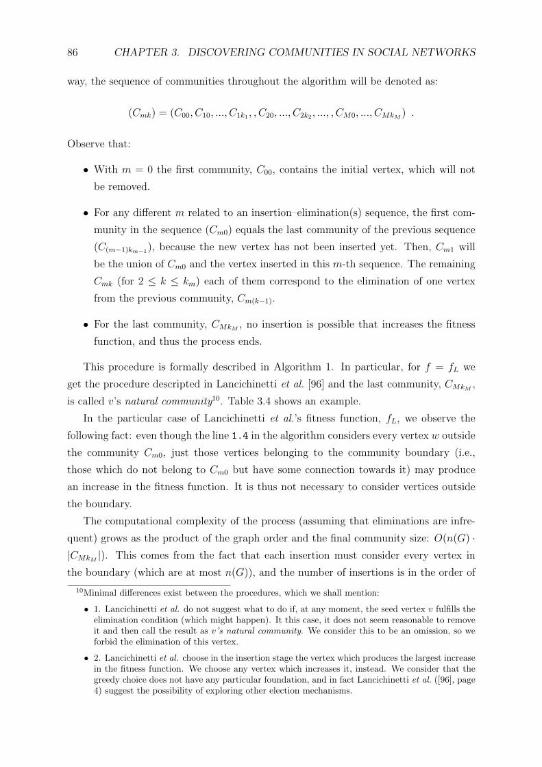
86 CHAPTER 3. DISCOVERING COMMUNITIES IN SOCIAL NETWORKS
way, the sequence of communities throughout the algorithm will be denoted as:
(Cmk) = (C00, C10, ..., C1k1 , , C20, ..., C2k2 , ..., , CM0, ..., CMkM ) .
Observe that:
• With m = 0 the first community, C00, contains the initial vertex, which will not
be removed.
• For any different m related to an insertion–elimination(s) sequence, the first com-
munity in the sequence (Cm0) equals the last community of the previous sequence
(C(m−1)km−1), because the new vertex has not been inserted yet. Then, Cm1 will
be the union of Cm0 and the vertex inserted in this m-th sequence. The remaining
Cmk (for 2 ≤ k ≤ km) each of them correspond to the elimination of one vertex
from the previous community, Cm(k−1).
• For the last community, CMkM , no insertion is possible that increases the fitness
function, and thus the process ends.
This procedure is formally described in Algorithm 1. In particular, for f = fL we
get the procedure descripted in Lancichinetti et al. [96] and the last community, CMkM ,
is called v’s natural community10. Table 3.4 shows an example.
In the particular case of Lancichinetti et al.’s fitness function, fL, we observe the
following fact: even though the line 1.4 in the algorithm considers every vertex w outside
the community Cm0, just those vertices belonging to the community boundary (i.e.,
those which do not belong to Cm0 but have some connection towards it) may produce
an increase in the fitness function. It is thus not necessary to consider vertices outside
the boundary.
The computational complexity of the process (assuming that eliminations are infre-
quent) grows as the product of the graph order and the final community size: O(n(G) ·|CMkM |). This comes from the fact that each insertion must consider every vertex in
the boundary (which are at most n(G)), and the number of insertions is in the order of
10Minimal differences exist between the procedures, which we shall mention:
• 1. Lancichinetti et al. do not suggest what to do if, at any moment, the seed vertex v fulfills theelimination condition (which might happen). It this case, it does not seem reasonable to removeit and then call the result as v’s natural community. We consider this to be an omission, so weforbid the elimination of this vertex.
• 2. Lancichinetti et al. choose in the insertion stage the vertex which produces the largest increasein the fitness function. We choose any vertex which increases it, instead. We consider that thegreedy choice does not have any particular foundation, and in fact Lancichinetti et al. ([96], page4) suggest the possibility of exploring other election mechanisms.

3.5. THE FGP METHOD 87
Algorithm 1: Natural communities
Input: A graph G, a fitness function f, an seed vertex v ∈ V (G)Output: A growth process C00, C10, . . . , Ca0, . . . , Caka , . . . , . . . , CMkM
1.1 begin1.2 D00 = v1.3 m = 01.4 while there exists some w out of Cm0 such that f(Cm0 + w) > f(Cm0) do1.5 Cm1 = Cm0 + w1.6 k = 11.7 while there exists some w ∈ Cmk, w 6= v : f(Cmk − w) > f(Cmk) do1.8 Cm(k+1) = Cmk − w1.9 k = k + 1
1.10 end1.11 C(m+1)0 = Cmk1.12 m = m+ 1
1.13 end
1.14 end
CMkM (under the hypothesis that eliminations are infrequent). In the worst case, the
computational cost of finding a natural community is of O(n(G)2). As the procedure in
Lancichinetti et al. must find a graph cover, the complexity can be bound as the product
between n(G)2 and the number of communities in the cover. This makes for a worst-
case complexity of O(n(G)3) when communities have great overlap, and a complexity of
O(n(G)2) when the overlapping is small.
3.5.2 Fitness functions
The work by Lancichinetti et al. suggests exploring other fitness functions in the con-
struction of natural communities. Here we shall deal with two parametric families of
fitness functions, based in our measures mV and cE (see Table 3.3):
Lt =mV − cEm
1/tV
(3.12)
Ht = mV (1−mV /2t)− cE , (3.13)
with t > 0. The first fitness function is proportional to the one in Lancichinetti et al.,
for α = 1/t. As we shall see, t plays the role of resolution parameter.
A differential analysis. We will show these two facts:
• In both fitness functions, Lt and Ht, changing the resolution parameter t does
not essentially affect the evolution of the growth process, but only defines the

88 CHAPTER 3. DISCOVERING COMMUNITIES IN SOCIAL NETWORKS
f(C
)=
din
(C)
din
(C)+dout(C
)=
0f
(C)
=din
(C)
din
(C)+dout(C
)=
26f
(C)
=din
(C)
din
(C)+dout(C
)=
49
f(C
)=
din
(C)
din
(C)+dout(C
)=
814
f(C
)=
din
(C)
din
(C)+dout(C
)=
14
21
f(C
)=
din
(C)
din
(C)+dout(C
)=
20
25
f(C
)=
din
(C)
din
(C)+dout(C
)=
24
29
f(C
)=
din
(C)
din
(C)+dout(C
)=
26
31
f(C
)=
din
(C)
din
(C)+dout(C
)=
28
33
Tab
le3.4:
The
natu
ralcom
mu
nity
ofa
vertexfor
α=
1.C
onstru
ctionof
the
natu
ralcom
munity
ofa
vertex,
accordin
gto
the
pro
cedure
descrip
tedin
Lan
cichin
ettiet
al..In
this
exam
ple,
no
elimin
ations
arenecessary.
The
natu
ralcom
munity
has
9vertices
and
afinal
fitn
essfu
nction
value
of28
33 .
Addin
gan
yvertex
into
the
final
comm
unity
wou
ldpro
duce
adecrease
inth
efitn
essfu
nction
value.

3.5. THE FGP METHOD 89
termination criteria. Vertices that are candidates for insertion or elimination under
some value of the resolution parameter, will remain candidates when the resolution
is decreased (i.e., when we obtain larger natural communities).
• Both fitness functions, Lt and Ht, are essentially equivalent, in the sense that
candidates for insertion or elimination for the Lt process are also candidates for
the Ht process.
In order to prove this, let us consider a community Cmk and some vertex w. If w 6∈Cmk then we shall consider vertex insertion, otherwise we shall consider its elimination.
In both cases we shall get a new community C+mk = Cmk ± w11.
Let us denote ∆mV = mV (C+mk)−mV (Cmk) and ∆cE = cE(C+
mk)− cE(Cmk), and let
us consider that s, t > 0 are two fixed values of the resolution parameter. Then we get
the following approximate expression for the difference quotient of Lt:
∆Lt∆mV
≈ L′t =1
m1/tV
(1− ∆cE
∆mV
− L1
t
).
For the difference quotient of Ht we obtain:
∆Ht
∆mV
≈ H ′t =
(1− ∆cE
∆mV
− mV
t
).
Notice then the following relations:
H ′t = H ′s +t− sts
mV (3.14)
m1/tV L′t = m
1/sV L′s +
t− sts
L1 (3.15)
H ′t = m1/tV L′t + (L1 −mV )/t . (3.16)
Equation (3.14) shows us that if t > s and H ′s > 0, then H ′t > 0, which means that
if the vertex w is a candidate for insertion into Cmk for the Hs function, then it is also
a candidate for insertion for the Ht function.
Equation (3.15) shows us analogously that if t > s and L′s > 0, then L′t > 0, which
means that if the vertex w is a candidate for insertion into Cmk for the Ls function, then
it is also a candidate for insertion for the Lt function.
This shows that the parameter t does not play an essential role during the growth
process for Ht or Lt, but merely establishes the termination criterion.
11We shall call C+mk to the element which follows Cmk in the sequence. Committing an abuse of
notation, we shall write Cmk + w instead of Cmk ∪ w, and Cmk − w instead of Cmk − w.

90 CHAPTER 3. DISCOVERING COMMUNITIES IN SOCIAL NETWORKS
Equation (3.16) shows a delicate fact: if a vertex w is a candidate for insertion
(elimination) for the Lt function and mV < L1 then it is a candidate for insertion
(elimination) for the Ht function. The condition mV < L1 is usually true; notice that
from mV > L1 it would follow that cE > mV (1 −mV ), which contradicts the notion of
community, because the second term would be the mean of the first one if the vertices
were to be selected randomly. Thus, both processes are essentially equivalent, their
difference lying in the termination criterion. There are approximations involved, so that
our previous comments are rough and qualitative, but our experience testing both fitness
functions confirms them.
3.5.3 The fitness growth process (FGP)
The described algorithm gets natural communities for different values of the t parameter.
We have seen that, as a general rule, the larger the t value, the larger the communities,
so that t behaves as a resolution parameter. It is reasonable to wonder whether it is
possible to obtain all these communities for different values of the resolution parameter
with a unique process. We shall see that this is indeed possible when using our Ht
function.
We shall call ∂(Cmk) to the boundary of Cmk, which is formed by those vertices which
lie outside of Cmk but have one or more connections to vertices in it.
Let us now consider a community Cmk and its boundary ∂(Cmk). We shall analyze
what happens when trying to insert into Cmk some vertex w in the boundary, or either
remove it in case it belongs to Cmk12. The updated fitness function value will be in each
case (±)
Ht(C ± w) = (mV + ∆mV )(1− (mV + ∆mV )/2t)− (cE + ∆cE)
= mV (1−mV /2t)− cE
−∆mV
t(mV + ∆mV /2) + ∆mV −∆cE
= Ht(C)− ∆mV
t(mV + ∆mV /2) + ∆mV −∆cE .
The variation of the fitness function is
∆Ht = −∆mV
t(mV + ∆mV /2) + ∆mV −∆cE ,
from where we observe that for t big enough (or small enough, according to ∆mV ’s sign),
12Those vertices which do not belong to Cmk nor its boundary are not considered, because ∆Ht isalways negative for them, for every t value.

3.5. THE FGP METHOD 91
∆Ht will be positive. The critical value of t is:
tc(Cmk, w) =∆mV (mV + ∆mV /2)
∆mV −∆cE.
It follows that if we are inserting w, then t > tc → ∆Ht > 0, whereas if we are eliminating
it, then t < tc → ∆Ht > 0.
Let us now suppose that when we reach the termination criterion of the natural
community for some resolution t, we increase this parameter as little as possible so
as to arrive at a new t′ = tc(Cmk, w) in which we can insert a new vertex w without
diminishing the value of Htc . The result will be a uniform growth process for Htc , where
tc is dynamically updated. If we extend this process till we span the whole graph, we
will get a sequence of natural communities (Cmk) at different resolutions.
Each natural community Cmk will have some associated resolution tmk, which will be
updated after each insertion, as:
t+mk = maxtmk, tc(Cmk, w) ,
where t+mk is the resolution of the new natural community C+mk = C+
mk ∪ w. The
sequence formed by the resolution values (tmk) will be a non-decreasing one, and each
community in the sequence C00, ..., Cmk will be a growth process for Ht, ∀t > tmk. The
sequence of natural communities (Cmk) built under this procedure is a uniform growth
process for H.
We describe this procedure in Algorithm 2.
3.5.4 Extracting the communities
Our hypothesis states that the uniform growth process will traverse the communities one
after the other until it spans the whole graph. In each step, the growth process tends to
choose the next vertex in terms of its cohesion with the natural community at that time.
Thus, two vertices which are consecutive in the process should either belong to the same
community or either be border vertices. Our community detection method includes a
technique for cutting the process into communities.
We consider the sequence of communities (Cmk) in which several insertions and elim-
inations are included. At the end of the sequence, the whole graph is contained into
the natural community. Then, every vertex must appear an odd number of times in the
sequence (k insertions and k − 1 eliminations). As a first step, we shall now keep only
the last insertion of each vertex. This insertion is the one which determines the vertex
position in a new sequence called S. In this sequence, each vertex appears just once.

92 CHAPTER 3. DISCOVERING COMMUNITIES IN SOCIAL NETWORKS
Algorithm 2: Uniform growth process for H
Input: A graph G, a seed vertex v ∈ V (G)Output: A uniform growth process for H:
C00, C10, . . . , Ca0, . . . , Caka , . . . , CM0, . . . , DMkM
2.1 begin2.2 C00 = v2.3 ta = 02.4 m = 02.5 while there exists some w ∈ ∂(Cm0) do2.6 let w0 be such that tc(Cm0, w0) = minw∈∂(Cm0)(tc(Cm0, w))2.7 ta = maxta, tc(Cm0, w0)2.8 Cm1 = Cm0 + w0
2.9 k = 12.10 while there exists some w ∈ Cmk, w 6= v : tc(Cmk, w) > ta do2.11 Cm(k+1) = Cmk − w2.12 k = k + 1
2.13 end2.14 C(m+1)0 = Cmk2.15 m = m+ 1
2.16 end
2.17 end
Thus, the sequence defines an ordering of the set V (G).
The conversion of this sequence S into a set of final communities C = (C1, C2, ..., CN)
is performed by observing the behavior of the following function:
S(w) =cE(C(w))
mV (C(w)), (3.17)
where the C(w) sets are subsequences of S, from the point in which the last community
was started, up to w. We will close a community and start a new one each time we
observe an increase in the function S(w).
In other words, the function S(w) considers the set of vertices since the beginning
of the last community, and computes the ratio of the normalized external community
degree (cE) to its normalized degree (mV ). In the next section, we shall offer a statistical
argument for the correct behavior of this cutting technique.
3.5.5 Behavior in the thermodynamic limit
In order to understand the statistical behavior of the function S(w), we shall consider a
community C = (v1, v2, ..., vn) whose vertices have a homogeneous mixing parameter µ.
That is, they share a fraction µ of their edges with other communities and a fraction 1−µ

3.5. THE FGP METHOD 93
with their own community C. We shall call Ci to the partial communities compressed
from v1’s insertion up to the insertion of some vi. The evolution of S(vi) will follow
Si = S(vi) =mE(Ci × (V \ Ci))
mV (Ci)= 1− L1(Ci) .
Our statistical analysis will be based in the following relations:
mE(Ci × (V \ C)) = µmV (Ci)
mE(Ci × Ci) = λimE(Ci × C) .
The first of them follows from the hypothesis that all the vertices in C share a similar
µ. The second is just a definition of a parameter λi which belongs to the interval [0, 1].
From these equations it can be shown, by a straightforward calculation and using the
additivity of mE, that
Si = µ+ (1− µ)(1− λi)
(1− µ)λi = L1(Ci) .
Here we assume that L1 has a monotone increasing behavior throughout the com-
munity construction13, and this implies a monotone decreasing behavior on Si also, even
without assuming a constant µ. We also observe that, for the last vertex in the commu-
nity, vn, it holds that S = µ (because λ = 1).
Now, let us see what happens when the community is finished and we incorporate
some vertex v from the following community, C ′, which has its own mixing parameter
µ′. We shall call C+ to C ∪ v, and we define ε by the relation
mE(v × C) = ε mE(v × (V \ C ′)) = εµ′mV (v) ,
which represents the proportion of external connections from v ∈ C ′ going to vertices in
C.
The new value for S is then:
S+ =mE(C+ × (V \ C+))
mV (C+)
13Let us recall that the fitness function L1 is related to the concept of community in a weak sense byRadicchi.

94 CHAPTER 3. DISCOVERING COMMUNITIES IN SOCIAL NETWORKS
and it can be shown that
S+ = µ+(1− 2εµ′ − µ)mV (v)
mV (C+).
If the mixing parameters are not very high (which would imply scarcely cohesive
communities) or either ε is small (which is expected) then this new value for S+ will
break the decreasing behavior of S producing the closure of C and the start of a new
community C ′ containing v′ as its first vertex, v′1.
We can now resume the behavior of S(w) in the following way:
• The function starts from S(w) = 1 when the first vertex of the community is
incorporated (w = v1).
• The function S(w) decreases from 1 up to µ throughout the community construc-
tion.
• The function S(w) will increase when the community is finished and the process
tries to incorporate an external vertex w′.
• Under this condition, a new community C ′ is started with that external vertex and
S(w′) is set to 1.
• Even in case that the mixing parameters of the vertices are not homogeneous,
the minimum of S(w) reached at the end of the community is still the average of
the mixing parameters of the vertices in the community, weighted by each own’s
degree, d(v). To this community mixing parameter we shall call µ(C).
Example: The football network. We shall illustrate the cutting technique in Fig-
ure 3.5 by picturing the evolution of the function S(v) throughout the growth process in
the football network. We clearly observe the function’s decreasing behavior inside each
community. Figure 3.4 visualizes the obtained community partition.
3.5.6 Computational complexity
In this section we shall prove that our community structure detection method has a com-
putational time complexity of O(n(G) · dmax + e(G) · log(n(G))), and a space complexity
of O(n(G) + e(G)).
We begin by analyzing the time complexity. Let us consider a community Cmk in the
process, and its associated parameter tmk. A new vertex is to be inserted. Line 2.6 in

3.5. THE FGP METHOD 95
0 20 40 60 80 100
0.4
0.6
0.8
1.0
Index for v in the growth process
S(v
)
Figure 3.4: The uniform growth process in the football network.
Algorithm 2 points out that we must insert that vertex w in the boundary of Cmk which
has the minimum tc(Cmk, w). We observe, from the expression of tc, that
tc(Cmk, w) =∆mV
∆mV −∆cE· (mV + ∆mV /2) .
From among the vertices in the boundary having the same degree as w, the one with
the minimum tc is the one that minimizes ∆mV∆mV −∆cE
. For a given degree, minimizing
this expression is the same as minimizing ∆cE, which is proportional to doutC − dinC . So,
if we group the vertices in the boundary into lists according to their degree, and we
order each list by increasing value of doutC − dinC , then we can assure that the vertex in
the boundary which minimizes tc must be at the head of one of these lists. Then we
propose to keep an updated structure with the boundary ∂(Cmk) (see Figure 3.6). We
shall need an analogous structure for the vertices in the community Cmk for speeding
the eliminations; this structure is also shown in the same figure. In this way we reduce
the complexity from analyzing the whole boundary into analyzing dmax vertices at most.
We shall call lmax to the maximum length of one list, and these lists will be imple-
mented with a direct access, ordered structure, as a map or tree. The operations of
insertion preserving order have complexity O(log(lmax)), while the access has complexity
O(1). We are now ready to analyze the complexity of the r-th step.
1. Looking for the vertex w with the minimum tc(Cmk, w) implies finding the minimum
between the heads of each of the lists. This has a complexity O(dmax).
2. Updating the structures involves:
(a) Removing w from its list in the ∂(Cmk) structure. Complexity O(1).
(b) Updating ∆cE for w to (−∆cE). Complexity O(1).
(c) Inserting w into the k(w)-list in the Cmk structure. Complexity O(log(lmax)).
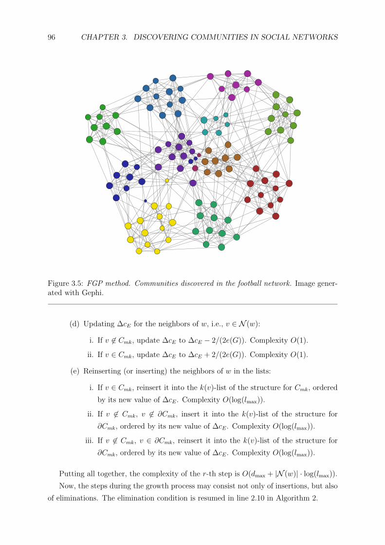
96 CHAPTER 3. DISCOVERING COMMUNITIES IN SOCIAL NETWORKS
Figure 3.5: FGP method. Communities discovered in the football network. Image gener-ated with Gephi.
(d) Updating ∆cE for the neighbors of w, i.e., v ∈ N (w):
i. If v 6∈ Cmk, update ∆cE to ∆cE − 2/(2e(G)). Complexity O(1).
ii. If v ∈ Cmk, update ∆cE to ∆cE + 2/(2e(G)). Complexity O(1).
(e) Reinserting (or inserting) the neighbors of w in the lists:
i. If v ∈ Cmk, reinsert it into the k(v)-list of the structure for Cmk, ordered
by its new value of ∆cE. Complexity O(log(lmax)).
ii. If v 6∈ Cmk, v 6∈ ∂Cmk, insert it into the k(v)-list of the structure for
∂Cmk, ordered by its new value of ∆cE. Complexity O(log(lmax)).
iii. If v 6∈ Cmk, v ∈ ∂Cmk, reinsert it into the k(v)-list of the structure for
∂Cmk, ordered by its new value of ∆cE. Complexity O(log(lmax)).
Putting all together, the complexity of the r-th step is O(dmax + |N (w)| · log(lmax)).
Now, the steps during the growth process may consist not only of insertions, but also
of eliminations. The elimination condition is resumed in line 2.10 in Algorithm 2.
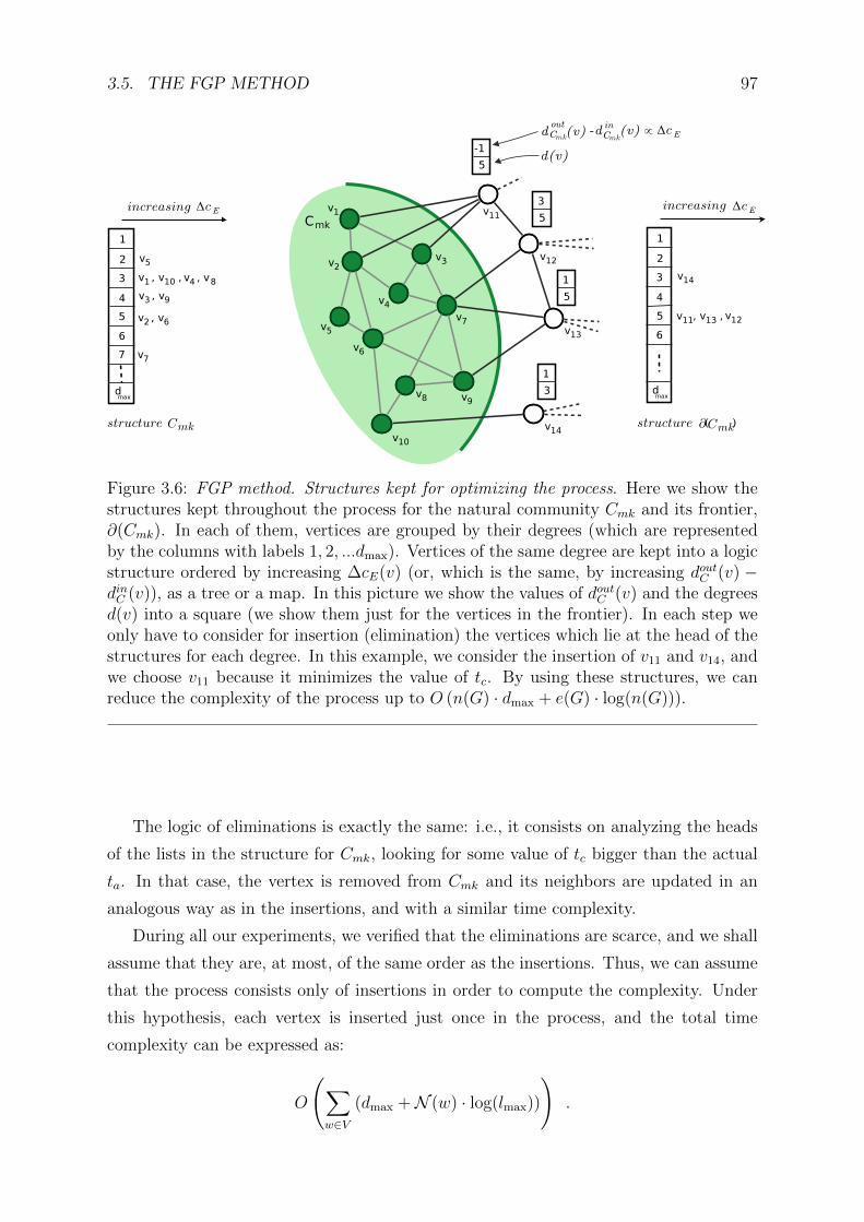
3.5. THE FGP METHOD 97
Figure 3.6: FGP method. Structures kept for optimizing the process. Here we show thestructures kept throughout the process for the natural community Cmk and its frontier,∂(Cmk). In each of them, vertices are grouped by their degrees (which are representedby the columns with labels 1, 2, ...dmax). Vertices of the same degree are kept into a logicstructure ordered by increasing ∆cE(v) (or, which is the same, by increasing doutC (v) −dinC (v)), as a tree or a map. In this picture we show the values of doutC (v) and the degreesd(v) into a square (we show them just for the vertices in the frontier). In each step weonly have to consider for insertion (elimination) the vertices which lie at the head of thestructures for each degree. In this example, we consider the insertion of v11 and v14, andwe choose v11 because it minimizes the value of tc. By using these structures, we canreduce the complexity of the process up to O (n(G) · dmax + e(G) · log(n(G))).
The logic of eliminations is exactly the same: i.e., it consists on analyzing the heads
of the lists in the structure for Cmk, looking for some value of tc bigger than the actual
ta. In that case, the vertex is removed from Cmk and its neighbors are updated in an
analogous way as in the insertions, and with a similar time complexity.
During all our experiments, we verified that the eliminations are scarce, and we shall
assume that they are, at most, of the same order as the insertions. Thus, we can assume
that the process consists only of insertions in order to compute the complexity. Under
this hypothesis, each vertex is inserted just once in the process, and the total time
complexity can be expressed as:
O
(∑w∈V
(dmax +N (w) · log(lmax))
).

98 CHAPTER 3. DISCOVERING COMMUNITIES IN SOCIAL NETWORKS
The sum over all the neighbors ofN (w) can be translated into the fact that every edge
in the network is considered only once. Regarding lmax, we cannot make any assumption.
In heavy-tailed degree distributions, the amount of vertices with a certain small degree
value may be close to O(n(G)), so we shall bound lmax with n(G). Thus, we have a
complexity of
O (n(G) · dmax + e(G) · log(n(G))) .
We shall also mention that in the initialization, the ∆cE’s and ∆mV ’s of the vertices
are both set to the their degrees. This step does not change the final complexity.
The cutting technique for obtaining a partition from the sequence S has a linear
complexity. It implies processing each element w ∈ S just once, computing the ratio
between cE and mV , which had already been obtained during the growth process.
In conclusion, the complexity of our method is dominated by the growth process
and is O (n(G) · dmax + e(G) · log(n(G))). By using appropriate data structures we man-
aged to reduce the original process complexity, which was of O(n(G)2). These same
structures might also improve the complexity of the covering algorithm by Lancichinetti
et al., whose original complexity lies between O(n(G)2) and O(n(G)3), as discussed in
Section 3.5.1.
Finally, regarding the spatial complexity, it is just of O(n(G) + e(G)), which is also
the spatial complexity of keeping the graph structure in memory. The data structures
on the community and its boundary just contain a degree list of size O(dmax), and a
set of dmax lists storing the information on the vertices for each vertex degree. For each
vertex, information of O(1) is kept, so the set of all lists has an extension of O(n(G)). As
we see, the spatial complexity of these two data structures does not exceed the spatial
complexity of the graph.
3.5.7 Results and data analysis
We have tested our community discovery method in some real networks and in instances
of random graphs generated with the LFR benchmark by Lancichinetti et al.. Thanks
to its low complexity and execution speed (which rivals that of known methods), our
method can be applied in networks of several millions of edges. We have made the source
code available for the scientific community at https://code.google.com/p/commugp/.
Next, we shall show the obtained results and we will produce comparisons with the
following methods:
• InfoMAP, by Rosvall and Bergstrom, based in the minimum description length [138].
• Louvain, by Blondel et al., an efficient greedy algorithm for modularity optimiza-
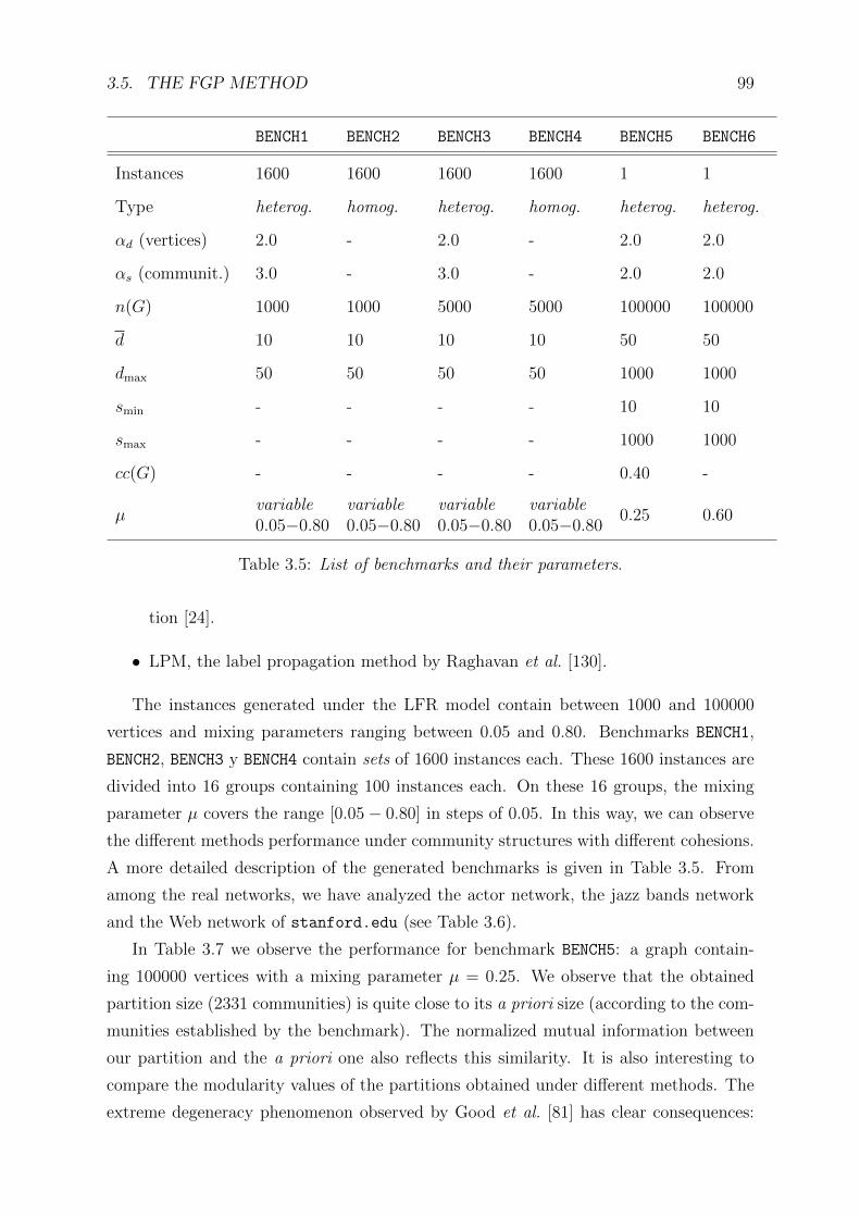
3.5. THE FGP METHOD 99
BENCH1 BENCH2 BENCH3 BENCH4 BENCH5 BENCH6
Instances 1600 1600 1600 1600 1 1
Type heterog. homog. heterog. homog. heterog. heterog.
αd (vertices) 2.0 - 2.0 - 2.0 2.0
αs (communit.) 3.0 - 3.0 - 2.0 2.0
n(G) 1000 1000 5000 5000 100000 100000
d 10 10 10 10 50 50
dmax 50 50 50 50 1000 1000
smin - - - - 10 10
smax - - - - 1000 1000
cc(G) - - - - 0.40 -
µvariable0.05−0.80
variable0.05−0.80
variable0.05−0.80
variable0.05−0.80
0.25 0.60
Table 3.5: List of benchmarks and their parameters.
tion [24].
• LPM, the label propagation method by Raghavan et al. [130].
The instances generated under the LFR model contain between 1000 and 100000
vertices and mixing parameters ranging between 0.05 and 0.80. Benchmarks BENCH1,
BENCH2, BENCH3 y BENCH4 contain sets of 1600 instances each. These 1600 instances are
divided into 16 groups containing 100 instances each. On these 16 groups, the mixing
parameter µ covers the range [0.05− 0.80] in steps of 0.05. In this way, we can observe
the different methods performance under community structures with different cohesions.
A more detailed description of the generated benchmarks is given in Table 3.5. From
among the real networks, we have analyzed the actor network, the jazz bands network
and the Web network of stanford.edu (see Table 3.6).
In Table 3.7 we observe the performance for benchmark BENCH5: a graph contain-
ing 100000 vertices with a mixing parameter µ = 0.25. We observe that the obtained
partition size (2331 communities) is quite close to its a priori size (according to the com-
munities established by the benchmark). The normalized mutual information between
our partition and the a priori one also reflects this similarity. It is also interesting to
compare the modularity values of the partitions obtained under different methods. The
extreme degeneracy phenomenon observed by Good et al. [81] has clear consequences:

100 CHAPTER 3. DISCOVERING COMMUNITIES IN SOCIAL NETWORKS
football jazz stanford.edu LiveJournal
n(G) 115 198 255265 4843953
e(G) 613 2742 1941926 42845684
d 10.66 27.70 15.21 17.69
dmax 12 100 38625 20333
cc(G) 0.403 0.633 0.653 0.351
Reference [76] [78] [103] [103]
Table 3.6: List of real networks and their parameters. All the networks have beenconsidered as undirected graphs.
qualitatively different partitions have very close modularity values (observe for example
the size of Louvain’s partition). The minimum description length also suggests a signi-
ficative difference between Louvain and the other methods, when compared with a trivial
partition. Finally, the community size distributions clearly show the consequences of the
resolution limit. While FGP, InfoMAP and LPM obtain community structures with
heterogeneous degree distributions (and quite close to that of the a priori partition),
Louvain is “forced” to obtain a community structure with more homogeneous commu-
nity sizes. Because of this, the Louvain partition has a smaller number of communities
as compared with the other methods. Table 3.8 also confirms these results for BENCH6,
whose mixing parameter is µ = 0.60.
Figure 3.7 uses a series of boxplots in order to show statistical values of the results
for the 4 benchmark sets with 1000 and 5000 vertices. Recall that each set contains
1600 graph instances in which the mixing parameter ranges between 0.05 and 0.80. The
boxplots reflect the normalized mutual information between the obtained partitions and
the a priori partitions, as a function of the mixing parameter µ. In Figure 3.8 we compare
our results with those of InfoMAP and Louvain. We observe that InfoMAP gets the best
results. In the same figure, we evidence that the modularity tends to generate small
partitions, and this tendency grows as the mixing parameter becomes larger.
Table 3.9 shows the results for a real network: the jazz bands network, formed by 198
bands whose connections point out that they have had some musician in common. As
we do not have a reference partition, we have compared the modularity, the minimum
description length, and the normalized mutual information between methods. Even
though the first two metrics are quite close for all methods (excepting Louvain) the
normalized mutual information reveals that the partitions are structurally different.
We have also analyzed a portion of the Web graph for the stanford.edu domain.

3.5. THE FGP METHOD 101
0.05 0.15 0.25 0.35 0.45 0.55 0.65 0.75
0.5
0.6
0.7
0.8
0.9
1.0
BENCH1, heterogeneous, n(G)=1000
Mixing parameter µ
Norm
aliz
ed m
utu
al in
form
ation
0.05 0.15 0.25 0.35 0.45 0.55 0.65 0.75
0.5
0.6
0.7
0.8
0.9
1.0
BENCH3, heterogeneous, n(G)=5000
Mixing parameter µ
Norm
aliz
ed m
utu
al in
form
ation
0.05 0.15 0.25 0.35 0.45 0.55 0.65 0.75
0.5
0.6
0.7
0.8
0.9
1.0
BENCH2, homogeneous, n(G)=1000
Mixing parameter µ
Norm
aliz
ed m
utu
al in
form
ation
0.05 0.15 0.25 0.35 0.45 0.55 0.65 0.75
0.5
0.6
0.7
0.8
0.9
1.0
BENCH4, homogeneous, n(G)=5000
Mixing parameter µ
Norm
aliz
ed m
utu
al in
form
ation
Figure 3.7: Results of the benchmarks BENCH1-4 (Part I). Normalized mutual informa-tion of the partitions obtained with the FGP method in the benchmarks BENCH1, BENCH2,BENCH3 and BENCH4, as a function of the mixing parameter µ. Each box contains statis-tical information on the 100 instances of the set with the same µ value. The horizontalline inside each box represents the median of the 100 samples, whereas the box extremescorrespond to the first and third quartile. The full interval (whiskers) spans all the rangeof samples.
This network contains 281903 web pages connected by 2312497 hyperlinks14. Table 3.10
shows the results.
The results on the LiveJournal network, with 5 million vertices, is particularly in-
teresting. Due to its size and hardware limitations, we only managed to process it with
FGP and Louvain. Table 3.11 shows that in both cases the community degree distribu-
tions follow a power-law. The resolution limit phenomenon is not observed for Louvain
in this case. This happens because the small communities are not connected among
them. Nonetheless, there are important differences. FGP detects 127058 communities,
whereas Louvain detects 8491. In FGP, the largest community contains 839473 vertices,
whereas in Louvain it contains 23993. Finally, we emphasize that the FGP partition
closely follows a power-law.
In order to visualize our observation relating how the communities in Louvain are
14We have only considered the biggest connected component, which contains the 90% of the pages.

102 CHAPTER 3. DISCOVERING COMMUNITIES IN SOCIAL NETWORKS
connected, we have considered the 8 largest communities (in terms of community degree,
d(C)) in Louvain’s partition, a the smallest ones (those with degree at most 5) and we
have visualized their connections with our software SnailVis [19]. Figure 3.10 shows that
the small communities are not connected among them.
In conclusion, we have shown that our FGP method, based on a uniform growth
process, obtains community structures from a local community notion. When the com-
munity degrees of the network follow heavy-tailed distributions, our method can detect
them, without presenting any resolution limit. In the LFR benchmarks our method in
surpassed by LPM and InfoMAP, while in real networks results are quite close. We con-
sider that one of the advantages of our method is its bounded complexity. Both in LPM
as in InfoMAP, it is difficult to perform a complexity analysis. In the former convergence
is not formally guaranteed, while in the latter heuristic methods are needed in order to
minimize the description length, and the computational complexity mostly depends on
the termination criterion.

3.5. THE FGP METHOD 103
FGP InfoMAP Louvain LPM a priori
|C| 2331 2346 314 2336 2346
MI(C, Capriori) 0.977 1.000 0.882 0.999 1.000
L(C) (min.desc. length.) 10.44 10.21 11.15 10.21 10.21
Q(C) (modularity) 0.708 0.731 0.727 0.731 0.731
JI(C, Capriori) 0.897 1.000 0.354 0.992 1.000
FCCV (C, Capriori) 0.920 1.000 0.000 0.945 1.000
µ(C) 0.298 0.252 0.249 0.252 0.252
d(C)
p(d
(C))
Community degree distribution
102
103
104
105
1061
0−
81
0−
71
0−
61
0−
51
0−
41
0−
31
0−
2
FGP
InfoMAP
Louvain
LPM
a priori
s(C)
p(s
(C))
Community size distribution
100
101
102
103
1041
0−
61
0−
51
0−
41
0−
31
0−
21
0−
11
00
FGP
InfoMAP
Louvain
LPM
a priori
Table 3.7: Results for benchmark BENCH5. (Up) Comparison among the partitions ob-tained by FGP, InfoMAP, Louvain and LPM for an instance of the LFR benchmarkcontaining 100000 vertices. The network description is given in Table 3.5. In order tointerpret the values of the minimum description length, we shall mention that, for atrivial partition in which all the vertices were in the same community, the minimumdescription length would be of 12.82. The last row, µ(C), represents the average mixingparameter of the communities in the partition. (Down) Community size distribution forthe partitions obtained with FGP, InfoMAP, Louvain and LPM, and for the a prioripartition. The distribution was adjusted with a logarithmic binning. The similarity inthe community size distribution for such diverse methods as FGP, InfoMAP and LPMis surprising.

104 CHAPTER 3. DISCOVERING COMMUNITIES IN SOCIAL NETWORKS
FGP InfoMAP Louvain LPM a priori
|C| 1878 2314 150 2104 2315
MI(C, Capriori) 0.914 0.999 0.814 0.989 1.000
L(C) (min.desc. length.) 14.09 13.56 14.37 13.61 13.56
Q(C) (modularity) 0.343 0.390 0.389 0.391 0.391
JI(C, Capriori) 0.635 0.978 0.189 0.814 1.000
FCCV (C, Capriori) 0.589 0.989 0.000 0.706 1.000
µ(C) 0.664 0.601 0.595 0.601 0.601
d(C)
p(d
(C))
Community degree distribution
102
103
104
105
1061
0−
81
0−
71
0−
61
0−
51
0−
41
0−
31
0−
2
FGP
InfoMAP
Louvain
LPM
a priori
s(C)
p(s
(C))
Community size distribution
100
101
102
103
1041
0−
61
0−
51
0−
41
0−
31
0−
21
0−
11
00
FGP
InfoMAP
Louvain
LPM
a priori
Table 3.8: Results for benchmark BENCH6. (Up) Comparison among the partitions ob-tained by FGP, InfoMAP, Louvain and LPM for an instance of the LFR benchmarkcontaining 100000 vertices. The network description is given in Table 3.5. (Down) Com-munity size distribution for the partitions obtained with FGP, InfoMAP, Louvain andLPM, and for the a priori partition. The distribution was adjusted with a logarithmicbinning.
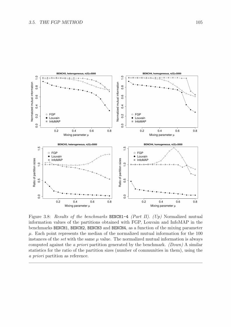
3.5. THE FGP METHOD 105
0.2 0.4 0.6 0.8
0.0
0.2
0.4
0.6
0.8
1.0
BENCH3, heterogeneous, n(G)=5000
Mixing parameter µ
Norm
aliz
ed m
utu
al in
form
ation
FGP
Louvain
InfoMAP
0.2 0.4 0.6 0.8
0.0
0.2
0.4
0.6
0.8
1.0
BENCH4, homogeneous, n(G)=5000
Mixing parameter µ
Norm
aliz
ed m
utu
al in
form
ation
FGP
Louvain
InfoMAP
0.2 0.4 0.6 0.8
0.0
0.5
1.0
1.5
BENCH3, heterogeneous, n(G)=5000
Mixing parameter µ
Ratio o
f part
itio
n s
izes
FGP
Louvain
InfoMAP
0.2 0.4 0.6 0.8
0.0
0.5
1.0
1.5
BENCH4, homogeneous, n(G)=5000
Mixing parameter µ
Ratio o
f part
itio
n s
izes
FGP
Louvain
InfoMAP
Figure 3.8: Results of the benchmarks BENCH1-4 (Part II). (Up) Normalized mutualinformation values of the partitions obtained with FGP, Louvain and InfoMAP in thebenchmarks BENCH1, BENCH2, BENCH3 and BENCH4, as a function of the mixing parameterµ. Each point represents the median of the normalized mutual information for the 100instances of the set with the same µ value. The normalized mutual information is alwayscomputed against the a priori partition generated by the benchmark. (Down) A similarstatistics for the ratio of the partition sizes (number of communities in them), using thea priori partition as reference.

106 CHAPTER 3. DISCOVERING COMMUNITIES IN SOCIAL NETWORKS
FGP InfoMAP Louvain LPM
|C| 2 5 4 3
L(C) (min.desc. length.) 6.93 6.92 6.87 6.93
Q(C) (modularity) 0.282 0.286 0.443 0.282
µ(C) 0.079 0.401 0.319 0.165
NMI FGP InfoMAP Louvain LPM
FGP 1.0000000 0.8310516 0.6048218 0.9531406
InfoMAP 0.8310516 1.0000000 0.5879541 0.8556317
Louvain 0.6048218 0.5879541 1.0000000 0.5866110
LPM 0.9531406 0.8556317 0.5866110 1.0000000
Table 3.9: Results obtained for the jazz bands network. (Up) Visualization of the parti-tion obtained with the FGP method. The visualization was generated with Gephi, andthe vertex positioning was performed with a force-directed method. Vertex colors repre-sent the assigned communities, and their sizes are proportional to the degree. (Center)Characterization of the partitions obtained by different methods. (Down) Comparisonmatrix for the partitions using the normalized mutual information.

3.5. THE FGP METHOD 107
Figure 3.9: FGP method. A community in the Web graph of stanford.edu. In thisfigure we show in green those vertices which belong to the community (excepting the bluevertex, which also belongs to it), and in white/gray the first networks of the community(i.e., vertices at distance 1 from it). We only draw the edges which are internal to thecommunity (dark green) and those connecting the community to its first neighbors (lightgreen), but we do not draw edges between community neighbors. The blue vertex is thefirst vertex in the community found by the process. Observe that it is a border vertex.The vertex sizes are proportional to their degrees. The vertices inside the communityhave a mean degree of 40 and a deviation of 10. The big vertices which are drawnlie between the 15 vertices of highest degree in the whole graph, their degrees rangingbetween 20000 and 40000. The picture was generated with Gephi, and the vertices werepositioned with a force-directed algorithm.

108 CHAPTER 3. DISCOVERING COMMUNITIES IN SOCIAL NETWORKS
FGP InfoMAP Louvain LPM
|C| 4173 5454 513 4678
L(C) (min.desc. length.) 10.13 9.15 10.47 9.66
Q(C) (modularity) 0.769 0.846 0.920 0.861
µ(C) 0.201 0.198 0.010 0.151
d(C)
p(d
(C))
Community degree distribution
100
101
102
103
104
105
1061
0−
81
0−
61
0−
41
0−
21
00
FGP
InfoMAP
Louvain
LPM
s(C)
p(s
(C))
Community size distribution
100
101
102
103
104
1051
0−
81
0−
61
0−
41
0−
21
00
FGP
InfoMAP
Louvain
LPM
Table 3.10: Results obtained for the Web graph of stanford.edu. (Up) Comparisonamong the partitions obtained by FGP, InfoMAP, Louvain and LPM. (Down) Com-munity size distributions for the partitions obtained with FGP, InfoMAP, Louvain andLPM. The distributions were adjusted with a logarithmic binning.

3.5. THE FGP METHOD 109
FGP Louvain
|C| 127058 8491
L(C) (min.desc. length.) 18.05 17.66
Q(C) (modularity) 0.304 0.727
µ(C) 0.551 0.126
d(C)
p(d
(C))
Community degree distribution
100
102
104
106
1081
0−
10
10
−8
10
−6
10
−4
10
−2
10
0
s(C)
p(s
(C))
Community size distribution
100
101
102
103
104
105
1061
0−
10
10
−8
10
−6
10
−4
10
−2
10
0
Table 3.11: Results obtained for the graph of the LiveJournal social network. (Up)Comparison among the partitions obtained by FGP and Louvain. (Down) Communitysize distributions for the partitions obtained with FGP (green) and Louvain (violet).The distributions were adjusted with a logarithmic binning.

110 CHAPTER 3. DISCOVERING COMMUNITIES IN SOCIAL NETWORKS
Figure 3.10: Communities obtained by Louvain in LiveJournal. Visualization of the8 biggest communities, those with degree at most 5, and the edge-cuts among them,in the partition of the LiveJournal social network obtained by Louvain. Each circlerepresents a community C, whose radius is proportional to the logarithm of its degree,d(C). The edge widths are proportional to the logarithm of the edge-cuts. We observethat, while the big communities almost form a clique among them, the small communitiesare not interconnected. The drawn communities may also have edges towards medium-sized communities, which are not drawn. The picture was generated with our softwareSnailVis [19].

Chapter 4
Connectivity in the Internet
In this chapter we shall address the study of the Internet as a complex system. We shall
begin by stating the technological relevance of its study, and by mentioning the most
important results up to now. In Section 4.2 we will present our contribution, which
relates the edge-connectivity of the network to the k-core decomposition, and we shall
apply it to recent Internet explorations.
4.1 Introduction
In its beginnings, the Internet was composed by a series of troncal connections referred
to as the backbone. Towards 1995, this backbone was the NSFNet, with 45 Mbps links
belonging to the United States government. In 1995 the NSFNet was shut down and the
Internet turned into being a completely decentralized network. Nowadays, the global
telecommunications companies provide network connectivity by means of their high-
speed links. Smaller companies buy the service from them, and resell it to the end
clients. This organization provides the Internet with certain hierarchical structure in
which some nodes are closer to the network center or backbone than others1.
Telecommunication companies in the different tiers have an autonomous internal
organization. From this autonomy, the concept of Autonomous System (AS) arises. An
Autonomous System of the Internet is a subnetwork which is under control of one or more
telecommunication companies, defining its own routing policy inside it. This means that
each Autonomous System controls the way in which routing is performed inside it, and
has a full vision of its own structure. The structure of an Autonomous System can be
1The concept of Tier, though rather diffuse in its definition, is related to this hierarchical structure.It is usually stated that an Internet Tier-1 network is a subnetwork of the Internet backbone. Tier-2networks connect to Tier-1s and use them to reach other parts of the network. At the same time, theyoffer their service to the other tiers. Lastly, Tier-3 networks purchase the service from the Tiers-2s.They also establish connections among them and are the usual Internet access providers for end users.
111

112 CHAPTER 4. CONNECTIVITY IN THE INTERNET
described as a network graph formed by routers (vertices) connected by links (edges).
We can thus distinguish between two levels of study of the Internet as a complex
network:
• The Autonomous Systems level (AS), in which nodes identify Autonomous Systems,
and edges correspond to links between routers in different ASes, which arise from
commercial agreements between them.
• The inter-router level (IR) , of higher level of detail, formed by routers and their
links.
At both levels it is quite useful to understand the rapport between network structure
and function. Some of the most important aspects of Internet’s study are:
• Latency: It consists of the communication delay between two nodes in the network.
It is related to propagation times in physical links, but mostly to the processing
delay at the nodes, which is seriously affected by congestion.
• Bandwidth: It is the amount of information transmitted between two nodes by
unit of time. Though it depends on the physical capacity of the links (which gets
higher and higher as new technologies develop), it is also enormously affected by
congestion.
• Robustness or resilience: It is the network capacity of tolerating a local failure
without serious effects on its global operation. A fundamental concept related to
robustness is redundancy, which is close to network connectivity, i.e., the multiplic-
ity of paths between the nodes.
• Topology: The Internet is a complex system. It presents scale-free distributions
and emergent behavior and it lacks of centralized control. In particular, the Inter-
net seems to be designed for maximizing fault tolerance (as the HOT mechanism
suggests) and information flow [126].
As we see, the Internet’s topology and its constitution as a complex system affect its
congestion and robustness. It is thus important to know the structure of the Internet
graph.
But the Internet is a dynamical network, and it is impossible to get a complete
snapshot of it. As it is not a centralized system either, no institution comes to have a
global register of its topology. Because of this, one of the initial problems in Internet’s
study was the network exploration.

4.1. INTRODUCTION 113
Internet explorations Nowadays, a couple of institutions perform this task. We shall
work with:
• CAIDA Association2: Explorations performed by the CAIDA association consist
of sending IP packets (called probes) from sites connected to the network (the
monitors) towards different destinations. As IP routing gives some information on
the path traversed by the packets, it is possible to use this information in order
to partially reconstruct the Internet graph. Up to now (July 2013) the system has
about 80 monitors around the world.
• DIMES Project3: It is a distributed system composed of nodes which voluntarily
cooperate. From each node, IP packets are sent with a low frequency. Up to now
(July 2013) it counts about 400 active agents, most of them in the United States.
• Route Views Project4: Whereas the previous methods send active probes, this
project performs passive measurements: it observes the BGP routing tables from
some AS border routers. As BGP stores the full path to reach other ASes, it is
possible to reconstruct the AS level topology of the Internet from these tables.
However, this method is biased as some routes between ASes are hidden (due to
private policies or agreements).
CAIDA and DIMES only provide information on the Internet router-level. But, as
the routers are identified by IP addresses which are publicly associated to the ASes, it is
possible to deduce the AS-level graph from the router-level one. In RouteViews, instead,
only an AS-level vision is provided, because the BGP tables only route between ASes.
Before these projects, the first works on Internet topology just observed a couple of
BGP tables. This is the case of Govindan and Reddy’s exploration [82] in 1997. In
this work, the authors showed that, despite the Internet’s growth during those years,
the diameter was quite stable. In 1998, Pansiot and Grad reconstructed the router-level
graph after sending IP packets among 11 routers in different parts of the world [124].
One year later, Govindan and Tangmunarunkit constructed a much more complete map
by exploiting the source-routing option of the IP protocol [83].
In 1999 Faloutsos et al. presented their well-known article showing the existence of
power-laws in some distributions of the Internet graph, as the vertex degree distribution
and the distance distribution [66]. In order to obtain these results, they analyzed some
2http://www.caida.org/home/ [34].3http://www.netdimes.org/new/ [56].4http://www.routeviews.org/ [150].

114 CHAPTER 4. CONNECTIVITY IN THE INTERNET
BGP tables provided by the NLANR5 and by the router-level exploration by Pansiot
and Grad [124].
The work by Faloutsos et al. had great impact. Pastor-Satorras et al. confirmed the
scale-free distributions observed in it, but they also detected a disassortative behavior
of the vertex degree distribution at the Autonomous Systems level [125]6. This result
is tightly related to the Internet’s structure: as Catanzaro et al. point out, combining
scale-free distributions with disassortative behavior avoids the obtention of a self-similar
structure, producing a hierarchical one, instead. The hierarchical structure of the Inter-
net is formed by hubs (densely connected nodes) which also connect to other hubs, and
peripheral nodes which connect among them by using the hubs.
This hierarchical structure of the Internet at the AS-level is part of some conceptual
models like the jellyfish by Siganos et al. (2006) [145] and the MEDUSA by Carmi et
al. (2007) [38]. Both of them model the network with a layered structure. The jellyfish
model is stricter regarding the edge-density inside layers: they must constitute cliques
or k-plexes (see their definition in Figure 3.1). The MEDUSA model, instead, is inspired
in the k-core decomposition, introduced in Section 2.1.3.4.
The k-core decomposition is a quite useful tool for studying Internet’s structure.
Alvarez-Hamelin et al. [7] showed that the k-cores of the Internet preserve the scale-
free behavior of the complete network: e.g., when observing the degree distribution
inside a k-core, a power-law is found with the same exponent as the one of the whole
network. The same results were obtained for the neighbor degree distribution and the
vertex clustering coefficient as a function of degree. Lastly, the authors also found a
disassortative behavior.
The k-cores are tightly related to connectivity. The works by Carmi et al. (2006) [37]
and Alvarez-Hamelin et al. (2008) [7] empirically showed that the k-cores in the Internet
AS-level graph are k-connected.
Our contribution in this chapter is to define sufficient conditions for guaranteeing the
core-connectivity of a network, defined as the k-edge-connectivity of each k-core. We
will show that these conditions are satisfied in the AS-level Internet graphs. The results
of this work are published in [6].
5National Laboratory for Advanced Network Research. The project which funded the Laboratoryended in 2006, its resources being transferred to the CAIDA project.
6The data analyzed by Pastor-Satorras et al. were also provided by NLANR.

4.2. CONNECTIVITY ESTIMATION USING K-CORES 115
4.2 Connectivity estimation using k-cores
Let us recall that the edge-connectivity of a graph G, κ′(G), is the minimum number of
edges to be removed for obtaining a disconnected graph, and it equals the capacity of
the minimum edge-cut (see Chapter 2, Section 2.1.2.2). A graph G is k-edge-connected
when κ′(G) ≥ k. Also, if G is k-edge-connected, then at least k edge-disjoint paths exist
between any pair of vertices in G.
4.2.1 Formalization
As a first step, we shall introduce an expansion theorem about distance:
4.2.1.1 An expansion theorem
Given a simple graph G, we shall define the distance between a vertex x ∈ V (G) and a
subset A ⊂ V (G), dG(x,A), as the minimum among all distances between v and vertices
in A. In other words, dG(x,A) is the distance between x and its closest vertex in A.
In this theorem we shall consider two non-empty disjoint subsets of V (G):(Fig.4.1.a) Q and C.
Let G′ be the graph induced by C ′ = Q ∪ C, denoted as G′ = G[C ′]7. We define the
contracted distance for vertices(Fig.4.1.b)
(Fig.4.1.c)
x, y ∈ Q as:
dC′/C(x, y) = mindG′[Q](x, y), dG′(x,C) + dG′(y, C) ,
and for vertices(Fig.4.1.d)
(Fig.4.1.e)
x ∈ C ′, y ∈ C as:
dC′/C(x, y) = dC′/C(y, x) = dG′(x,C) .
With these definitions, our notion of contracted distance is defined for every pair of
vertices in C ′8.
We also define the contracted distance between a vertex x ∈ C ′ and a subset A ⊂ C ′,
as:
dC′/C(x,A) = mina∈A
dC′/C(x, a) .
Lastly, we introduce the notion of(Fig.4.1.f) contracted diameter of G′ = G[C ′] with respect to C
as
diamC′/C = maxx,y∈C′
dC′/C(x, y) .
7C will later represent a more central k-core which will provide connectivity to Q.8Its designation as contracted distance can be understood as the usual distance G′ considering that
the set C collapses into a unique vertex, which is connected to those vertices in Q which were previouslyneighbors of some vertex in C.

116 CHAPTER 4. CONNECTIVITY IN THE INTERNET
(a) A graph G′, induced by C ′ = C ∪Q. (b) Two vertices in Q whose contracteddistance is 2.
(c) Two vertices in Q whose contracted dis-tance is 1.
(d) The contracted distance between theblack vertex and any vertex in C is 2.
(e) The contracted distance between ver-tices in C is always 0.
(f) The contracted diameter of G′ is 3.
Figure 4.1: The notion of contracted distance.
With these definitions, it holds that if dC′/C(x, y) = 2 for some vertex pair x, y ∈ C ′,
then there exists some z ∈ C ′ such that dC′/C(x, z) = dC′/C(z, y) = 1.

4.2. CONNECTIVITY ESTIMATION USING K-CORES 117
(a) The border set ∂1Q. (b) The border set ∂2Q.
Figure 4.2: Border sets in Q.
We shall also use the following notation:9
∂jQ = x ∈ Q : |[x,C]| ≥ j
∂jQ = x ∈ Q : |[x,C]| < j = Q \ ∂jQ .
(Fig.4.2.a)
(Fig.4.2.b)
These nested sets ∂jQ organize the border vertices in Q according to the number of
connections they have with C.
Lastly, we shall consider:
ΦC′/C =∑x∈Q
minmax1, |[x, ∂2Q]|, |[x,C]|
Now we are ready for formulating our theorem.
Theorem 1. Given a simple graph G′ such that V (G′) = C ′ and C ⊂ C ′, if diamC′/C ≤2, then for every edge-cut [S, S] in G′ such that C ⊂ S it holds that:
1. If maxs∈S dC′/C(s, S) = 1, then |[S, S]| ≥ maxs∈S d(s).
2. If maxs∈S dC′/C(s, S) = 1, then |[S, S]| ≥ |S|.
3. If maxs∈S dC′/C(s, S) = 2, then |S| > mins∈S d(s).
4. If maxs∈S dC′/C(s, S) = 2, then maxs∈S dC′/C(s, S) = 1.
5. If maxs∈S∩Q dC′/C(s, S) = 1, then |[S ∩Q, S]| ≥ maxs∈S∩Q(d(s)− dC(s)).10
6. If maxs∈S∩Q dC′/C(s, S) = 1, then |[S ∩Q, S]| ≥ |S ∩Q|.9We shall commit a small abuse of notation in writing |[x,C]| instead of |[x, C]|.
10Our notation dC(s) denotes the internal degree of s in C, according to the notation introduced forcommunity structure in Chapter 3. It equals the number of edges going from s to vertices in C.

118 CHAPTER 4. CONNECTIVITY IN THE INTERNET
Proof.
1. (Fig.4.3.a)
(Fig.4.3.b)
Consider some s ∈ S. We split s’s degree into two components: dS(s) = |[s, S]| and
dS(s) = |[s, S]|. For each one of s’s neighbors in S, the edge-cut |[S, S]| is increased
by 1. Now, for each one of s’s neighbors in S the edge-cut is also increased by 1, as
its contracted distance to S is 1 (which means that it must have an edge to some
vertex in S). Then: |[S, S] ≥ dS(s) + dS(s) = d(s). As this holds for any s ∈ S,
we have that |[S, S]| ≥ maxs∈S d(s)
2. (Fig.4.3.c)This follows immediately if we note that for each s ∈ S there exists at least one
edge to S, and this edge increases the edge-cut [S, S] by 1.
3. (Fig.4.3.d)
(Fig.4.3.e)
In this case, there exists at least one vertex s ∈ S without any edge to S. For this
vertex, s, it holds that dS(s) = d(s). Then: |S| ≥ d(s) + 1 > mins∈S d(s).
4. (Fig.4.3.f)Following the reasoning in the previous item, if s does not have any edge to S then
the minimum path to reach s from any vertex s ∈ S has length 2 (because the
contracted diameter is less than or equal to 2) and the halfway vertex must belong
to S. Then, d(s, S) = 1.
5. If vertices in S which belong to Q have at least one edge to S, then using an
argument similar to that in item 1, we have that for each s ∈ S ∩ Q the edges
which do not arrive to C will arrive to S or either to other neighbors in S ∩ Q,
which also have at least one edge to S. Then, d(s) − dC(s) is a lower bound for
|[S ∩Q, S]|.
6. As in item 2, this is immediate if we observe that for each s ∈ S ∩ Q there exists
at least one edge to S.

4.2. CONNECTIVITY ESTIMATION USING K-CORES 119
(a) A graph G′, induced by C ′ = C ∪ Q,whose contracted diameter is 2, and anedge-cut [S, S] such that C ⊂ S. For everys ∈ S it holds that dC′/C(s, S) = 1.
(b) Item 1. s’s degree is a lower bound for|[S, S]|.
(c) Item 2. S’s cardinal is also a lowerbound for |[S, S]|.
(d) Here we modify some connections ofthe vertices in Q. The contracted diameteris still 2, but now we have some vertices inS without any edge to S. For every s ∈ Sit holds that dC′/C(s, S) ≤ 2.
(e) Item 3. s does not have any edge to S.Then, s’s degree plus 1 is a lower boundfor S’s cardinal.
(f) Item 4. Every vertex S is at a con-tracted distance of 2 from s. Then, everyvertex in S is at a contracted distance of 1from S.
Figure 4.3: Illustration of Theorem 1.

120 CHAPTER 4. CONNECTIVITY IN THE INTERNET
Corollary 1. Let us assume that in addition to the hypotheses of Theorem 1 it holds
that
|[S, S]| < minv∈Q
d(v) .
Then:
1. maxs∈S dC′/C(s, S) = 2.
2. maxs∈S dC′/C(s, S) = 1.
3. |[C, S]| ≥ 1.
4. |S ∩Q| < |[S, S]| < minv∈Q d(v) < |S|.
5. S ∩Q ⊂ ∂2Q or, which is the same, ∂2Q ⊂ S.
6. ΦC′/C ≤ |[S, S]|.
Proof.
1. (Fig.4.4.a)
(Fig.4.4.b)
This is a consequence of Item 1 in Theorem 1. Otherwise, vertices in S would have
an edge in the edge cut, and its capacity would be greater than or equal to the
degree of each vertex s.
2. (Fig.4.4.c)This is a consequence of Item 4 in Theorem 1 and our new hypothesis.
3. (Fig.4.4.d)Otherwise, every vertex in s ∈ S would have an edge to S ∩Q, and it would follow
that |[S, S]| ≥ d(s).
4. From Items 3 and 4 the first inequality follows. The second one is just the hypoth-
esis of this Corollary, and the third one comes from Item 3 in Theorem 1.
5. From Item 5 in Theorem 1 and Item 3 in this Corollary, it follows that:
|[S, S]| = |[S ∩Q, S]|+ |[C, S]| > maxs∈S∩Q
(d(s)− dC(s))
Then, for every s ∈ S ∩Q, our hypothesis implies that:
d(s) > |[S, S]| > (d(s)− dC(s))
from where it follows that dC(s) ≥ 2, and thus we conclude that every vertex in
S ∩Q belongs to the border set ∂2Q.

4.2. CONNECTIVITY ESTIMATION USING K-CORES 121
(a) A graph G′, induced by C ′ = C ∪ Q,with contracted diameter 2, and an edge-cut [S, S] such that C ⊂ S. The additionalhypothesis |[S, S]| < minv∈Q d(v) holds.
(b) Item 1. d(s, S) = 2.
(c) Item 2. Vertices in S ∩ Q must havesome edge to S.
(d) Item 3. The capacity of the edge-cut[C, S] is at least 1.
Figure 4.4: Illustration of Corollary 1.
6. As ∂2Q ⊂ S, for every s ∈ S ∩Q it holds that:
|[s, S]| ≥ max1, |[s, ∂2Q]|
whereas for s ∈ S it holds that |[s, S]| ≥ |[s, C]|. Then:
|[S, S]| = |[S ∩Q, S]|+ |[C, S]|
≥∑s∈S∩Q
max1, |[s, ∂2Q]|+∑s∈S
|[s, C]|
≥ ΦC′/C

122 CHAPTER 4. CONNECTIVITY IN THE INTERNET
Now we shall use Theorem 1 and Corollary 1 in order to establish a result on the
k-edge connectivity of a graph G′.
Corollary 2. Let k ≤ dmin(G′). If it holds that:
1. G′[C] is dmin(G′)-edge-connected
2. diamC′/C ≤ 2
Then any of the following conditions implies that G′ is k-edge-connected:
1. ΦC′/C ≥ k
2. |∂1Q| ≥ k
3. Q = ∂1Q
Proof. Let [S, S] be an edge-cut in G′. We will show that, under the 2 hypothesis and
any of the 3 alternatives, it holds that |[S, S]| ≥ k.
As a first case, let us suppose that C is split by the edge-cut, i.e.: S ∩ C 6= ∅ and
S ∩C 6= ∅. Then the edge-cut [S ∩C, S ∩C] is included in ⊂ [S, S]. But, as we assumed
that G′[C] is k-edge-connected, it follows that:
|[S, S]| ≥ |[S ∩ C, S ∩ C]| ≥ k
Then, let us suppose that C ⊂ S (without loss of generality; just for using the same
notation as in our previous results). If it held that |[S, S]| < k, then as k ≤ dmin(G′) ≤minv∈Q d(v), the first hypothesis in Corollary 1 would hold.
Nonetheless, the first of the conditions contradicts Item 6 in Corollary 1.
If v ∈ ∂1Q instead, then v has some edge to C. Then, v increases ΦC′/C by at least 1.
Now the second of our conditions implies the first one which, as we showed, contradicts
the Corollary.
Lastly, if Q = ∂1Q then every vertex in Q will have some edge to C, which contradicts
Item 1 in the Corollary.
Notation. In order to summarize the three conditions of Corollary 2, we shall use the
following notation:
ΨC′/C(k) = maxΦC′/C − k, |∂1Q| − k, |∂1Q| − |Q|, for k ≤ dmin(G′) .
Then, the 3 conditions can be summarized as: ΨC′/C(k) ≥ 0.

4.2. CONNECTIVITY ESTIMATION USING K-CORES 123
Observation: Our Corollary 2 is closely related to Plesnık’s theorem [127], which
states that in simple graphs of diameter 2 the edge-connectivity is equal to the minimum
degree. In fact, the condition of having a contracted diameter of 2 assures that the
graph obtained from G′ by contracting C into a vertex would be k-edge connected for
k ≤ dmin(G′). However, this is not enough for guaranteeing k-edge-connectivity, and
some of our 3 additional conditions is required.
4.2.1.2 Strict-sense and wide-sense edge-connectivity
Here we expand our notion of edge-connectivity for subgraphs induced by subsets A ⊂V (G).
We shall say that an induced subgraph G[A] is k-edge-connected in the strict sense
just when G[A] is k-edge-connected, i.e., when every edge-cut in G[A] has at least k
edges or, which is the same, at least k pairwise edge-disjoint paths exist for any vertex
pair u, v in G[A].
We shall say that an induced subgraph G[A] is k-edge-connected in the wide sense
when every edge-cut [X, X] in G which splits the A set –i.e., such that X ∩ A 6= ∅ and
X ∩ A 6= ∅– has at least k edges. This is the same as requiring the existence in the full
graph G of at least k pairwise edge-disjoint paths for any vertex pair u, v in A.
It immediately follows that if G[A] is k-edge-connected in the strict sense, then it is
also k-edge-connected in the wide sense.
4.2.1.3 Building core-connected sets
We will now relate our notions of edge-connectivity in the strict and wide sense with the
k-core decomposition. Let us recall that a k-core is an induced subgraph with minimum
degree k, which is maximal with respect to this property (see Section 2.1.3.4). Our
hypothesis here is that the k-cores are usually k-edge-connected. We shall design an
algorithm for traversing the k-cores, from the most central to the most peripheral ones.
This algorithm constructs a subset C ⊂ V (G) such that the k-cores of the subgraph
induced by C are k-edge-connected in the strict (wide) sense. We shall call this property
as core-connectivity in the strict (wide) sense:
Definition. A graph is core-connected in the strict (wide) sense when all of its k-cores
are k-edge-connected in the strict (wide) sense.
We expect the whole graph G to verify core-connectivity. But when this is not pos-
sible, the algorithm will extract a core-connected induced subgraph as large as possible.

124 CHAPTER 4. CONNECTIVITY IN THE INTERNET
Figure 4.5: k-shells and clusters in a graph. The graph in this example has core number5. The central k-core in included inside the 4-core (blue+light blue). Vertices belongingto the 4-core but not to the 5-core form the 4-shell (light blue). The 4-shell has 5connected components (clusters). The 4-core is contained inside the 3-core (blue+lightblue+green). The 3-shell (green) is composed of 4 clusters.
Core-connectivity in the strict sense The algorithm needs an initial subset with
large edge-connectivity, so it analyzes the more central k-core, and verifies the diameter-2
condition of Plesnık’s theorem. In order to verify this, the kmax-core must have a single
connected component. Otherwise, each component will be considered separately.
If no connected component is found which verifies the diameter-2 condition in the
kmax-core, then the algorithm advances to the next core, and considers the vertices in
the (kmax − 1)-core which do not belong to the kmax-core. This “crust” of a k-core is
called a k-shell (see Figure 4.5). The k-shell is the subgraph induced by the vertices with
shell index equal to k. Each k-shell may be composed of several connected components,
which are called clusters. The algorithm processes each k-shell until finding a first cluster
verifying the diameter-2 condition, and with minimum degree at least k. The vertices in
this cluster will form the initial C set. As the cluster is k-edge-connected for k equal to
its k-shell, the graph G[C] will be core-connected.
Once this first stage is over, the algorithm tries to append other clusters to C11. It
begins with the k-shell which immediately follows the one of the first cluster, and its
checks the conditions in Corollary 2 for each cluster in this k-shell. The cluster will
play the role of Q in the Theorem, whereas the C set satisfies the required hypothesis
of k-edge-connectivity12. In order to apply the Theorem in G[C ′], with C ′ = C ∩Q, the
11Observe that, as new vertices are added into C, the edge-connectivity of G[C] will decrease, butG[C] will always be core-connected.
12As C is core-connected and its minimum degree is at least the actual k, then C es k-edge-connected.

4.2. CONNECTIVITY ESTIMATION USING K-CORES 125
Algorithm 3: Core-connectivity in the strict sense
Input: Sk[G] = Qk1, Qk2, ..., QkMk, the k-shells of G (from 1 to kmax), split into
their connected components (clusters)Output: C ⊂ V , core-connected in the strict sense
3.1 C ← ∅3.2 k ← kmax3.3 begin3.4 while C = ∅ and k ≥ 1 do3.5 if there exists some Q ∈ Sk[G] satisfying diam(G[Q]) ≤ 2 and
dmin(G[Q]) ≥ k then3.6 C ← C ∪Q3.7 end3.8 k ← k − 1
3.9 end3.10 while k ≥ 2 do
3.11 while there exists some Q ∈ Sk[G] satisfying:
diamC∪Q/C ≤ 2ΨC∪Q/C(k) ≥ 0
]do
3.12 C ← C ∪Q3.13 Sk[G]← Sk[G] \Q3.14 end3.15 k ← k − 1
3.16 end3.17 for each Q ∈ S1[G] do3.18 if |∂1Q| ≥ 1 then3.19 C ← C ∪Q3.20 end
3.21 end
3.22 end
algorithm checks the 3 conditions in Corollary 2. If any of them holds, then the cluster
is added to C13.
The procedure traverses all the k-shells considering each cluster, until processing the
2-layer. For the 1-layer, our conditions are unnatural, and we simply have to verify that
the clusters in the 1-layer have at least one edge to C.
The final result is a subgraph G[C] satisfying core-connectivity, i.e., whose k-cores
are k-edge-connected. The computational time complexity of the algorithm is O(e(G))
(see [6]).
The full procedure is described in Algorithm 3.
13When Q is added, C will have minimum degree k and will be k-core-connected. But as the (k + 1)-core of C does not include any of the vertices in Q, then its keeps its previous edge-connectivity value.Thus, C is still core-connected.

126 CHAPTER 4. CONNECTIVITY IN THE INTERNET
Core-connectivity in the wide sense This procedure is shown in Algorithm 4.
Now the algorithm needs a buffer B in which we keep those clusters which could not
be added to C. If any time later some cluster verifies the conditions in line 4.15, then
the cluster is added to a set D. These belatedly added clusters have a connectivity in
G[C ∪D] which is smaller than their shell index. However, the value of k of the step in
which they were added assures the k-edge-connectivity of G[C∪D], which is the required
hypothesis on G[C∪D] in order to apply the theorem. So, the vertices in D are not part
of the core-connected set (only those in C are), but they can be used by other clusters
in order to establish their paths. The connectivity thus obtained is a connectivity in the
wide sense, as the paths connecting vertices in C may use vertices in the D set.
4.2.2 Results and data analysis
We applied our algorithms to the analysis of core-connectivity in Internet AS-level
graphs. The data was obtained from explorations by CAIDA and DIMES, and are
summarized in Table 4.1.
In Table 4.2 we show the number of nodes of the core-connected subgraphs extracted
from both algorithms. We observe that most vertices belong to the core-connected
subgraph. For each pair of vertices in this subgraph we can assure a minimum value of
edge-connectivity as the minimum between the shell indexes of the vertices.
We also compared our lower bound for edge-connectivity with the real edge-connectivity
in the graph. These results are shown in Figures 4.7 and 4.8. In these pictures, every
pair of vertices is considered. The pairs are organized on the x-axis according to min-
imum shell index. For each value of minimum shell index, the segment on the y-axis
shows the mean and standard deviation for the edge-connectivity of pairs with such
value of minimum shell index. Edge-connectivity is computed in two fashions: as the
edge-connectivity inside the deepest k-core containing both vertices (which we call edge-
connectivity through the core) and as the edge-connectivity in the full graph. For both
cases, we also show the curve f(x) = x corresponding to the edge-connectivity lower
bound guaranteed by our algorithm for those vertices belonging to the C set. We con-
clude that our lower bound is quite close to the edge-connectivity through the core.
The computation of the real edge-connectivity was made using a Gomory-Hu tree of
the full graph or either of each k-core (in the case of the edge-connectivity through the
core). The procedure is briefly described in the next lines.

4.2. CONNECTIVITY ESTIMATION USING K-CORES 127
4.2.2.1 Gomory-Hu trees
Edge-connectivity in graphs is related to the minimum edge-cut by Menger’s theorem
for edges (see page 30). This implies that the edge-connectivity can be computed using
the maximum flow algorithm by Ford-Fulkerson, with unitary weights in the edges. By
recursively applying this algorithm, Gomory and Hu showed that it is possible to build
an edge-weighted tree containing all the information on connectivity in the graph [80].
Figure 4.6 shows a Gomory-Hu tree for a simple graph. The edge-connectivity be-
tween any two vertices v and w equals the minimum among the capacities of the edges
in the path which connects both vertices.
Figure 4.6: Computing edge-connectivity with Gomory-Hu trees. On the left, we show asimple graph. On the right, an associated Gomory-Hu tree. This tree contains all theinformation on edge-connectivity for every pair of vertices v and w. In particular, theminimum among the capacities of the edges equals the edge-connectivity of the graph.

128 CHAPTER 4. CONNECTIVITY IN THE INTERNET
mincK(u),cK(v)
κ(u
, v)
5 10 15 20
10
01
01
10
21
03
mincK(u),cK(v)
κ(u
, v)
5 10 15 20
10
01
01
10
2Figure 4.7: Edge-connectivity in the AS-CAIDA 2013 network. The figure on the leftshows the edge-connectivity between every vertex pair u, v in the network, as a functionof minimum shell index, mincK(u), cK(v). On the right we plot the edge-connectivitythrough the core, i.e., the edge-connectivity inside the deepest core containing bothvertices. The continuous line represents the function f(x) = x. Vertical segmentsrepresent mean values and standard deviation. We observe that the minimum shell indexis quite close to the edge-connectivity through the core. The real edge-connectivity wascomputed by previously constructing the Gomory-Hu tree of the graph [80].
mincK(u),cK(v)
κ(u
, v)
5 10 15 20 25 30 35
10
01
01
10
21
03
mincK(u),cK(v)
κ(u
, v)
5 10 15 20 25 30 35
10
01
01
10
2
Figure 4.8: Edge-connectivity in the AS-DIMES 2011 network. Edge-connectivity (Left)and edge-connectivity through the core (Right) for every vertex pair u, v in the net-work, as a function of the minimum shell index of the pair, mincK(u), cK(v). For moredetails, see the caption on Figure 4.7.

4.2. CONNECTIVITY ESTIMATION USING K-CORES 129
Algorithm 4: Core-connectivity in the wide sense
Input: Sk[G] = Qk1, Qk2, ..., QkMk, the k-shells of G (from 1 to kmax), split into
their connected components (clusters)Output: C ⊂ V , core-connected in the wide sense
4.1 C ← ∅4.2 D ← ∅4.3 B← ∅4.4 k ← kmax4.5 begin4.6 while C = ∅ and k ≥ 2 do4.7 if there exists some Q ∈ Sk[G] satisfying diam(G[Q]) ≤ 2 and
dmin(G[Q]) ≥ k then4.8 C ← C ∪Q4.9 Sk[G]← Sk[G] \Q
4.10 end4.11 B← B ∪ Sk[G]4.12 k ← k − 1
4.13 end4.14 while k ≥ 2 do
4.15 while there exists some Q′ ∈ B satisfying:
diam(C∪D∪Q′)/(C∪D) ≤ 2Ψ(C∪D∪Q′)/(C∪D)(k) ≥ 0
]do
4.16 D ← D ∪Q′4.17 B← B \ Q′4.18 end
4.19 while there exists some Q ∈ Sk[G] satisfying:
diam(C∪D∪Q)/(C∪D) ≤ 2Ψ(C∪D∪Q)/(C∪D)(k) ≥ 0
]do
4.20 C ← C ∪Q4.21 Sk[G]← Sk[G] \ Q4.22 end4.23 B← B ∪ Sk[G]4.24 k ← k − 1
4.25 end4.26 for each Q ∈ S1[G] do4.27 if |∂1Q| ≥ 1 then4.28 C ← C ∪Q4.29 end
4.30 end
4.31 end

130 CHAPTER 4. CONNECTIVITY IN THE INTERNET
AS-CAIDA
2009
AS-CAIDA
2011
AS-CAIDA
2013
AS-DIMES
2011
n(G) 16117 19895 23779 26083
e(G) 32847 44560 54752 83305
d 4.08 4.48 4.61 6.39
dmax 2012 2465 2818 4517
kmax 16 20 24 35
cc(G) 0.013 0.014 0.016 0.015
Table 4.1: List of analyzed Internet graphs. For more details on the statistics of thesegraphs, consult Appendix B.
|V (G)| |V (G) \ Cstrict| |V (G) \ Cwide|
AS-CAIDA 2009 16117 145 94
AS-CAIDA 2011 19895 111 72
AS-CAIDA 2013 23779 28 24
AS-DIMES 2011 26083 45 34
Table 4.2: Core-connectivity of Internet graphs. Our algorithm obtains a core-connectedsubgraph G[C]. Core-connectivity implies that every k-core in this subgraph is k-edgeconnected. This table shows in its second column the number of vertices in the explo-ration graph. The next columns represent the number of vertices which could not beadded into the core-connected graph in the strict sense and in the wide sense, respec-tively.

4.3. VISUALIZING INTERNET CONNECTIVITY 131
4.3 Visualizing Internet connectivity
We used the visualization tool LaNet-vi [5] in order to visualize the k-core decomposition
of Internet graphs. From version 2.2.0 onwards, LaNet-vi incorporates an option for
finding core-connected subgraphs in the strict sense and in the wide sense, using the
algorithms presented here.
Figures 4.9 and 4.10 show the k-core decomposition of the AS-CAIDA 2011 and
AS-DIMES 2011 networks. Vertices which do not belong to the core-connected graph
in the strict sense are drawn in black. We observe just a few of them, in the peripheral
layers.
Figure 4.9: k-core decomposition and core-connected set in the strict sense for theAS-CAIDA 2011 network. The scale on the left represents vertex degree, and the oneon the right represents its shell index.
These pictures also reveal that the AS-level of the Internet has a high core number,
which increases year after year. Between the explorations in 2009 and 2013 the core
number increased from 16 to 24. Figure 4.11 shows the evolution of the maximum core
of the Internet between 2009 and 2013. The labels show that most of the ASes which
were in the center of the network in 2009 remain there in 2013, but many new ASes were
added. The ASes in this core are the most important providers of connectivity in the
Internet.
Lastly, we observe that the explorations by DIMES have more detail than those by

132 CHAPTER 4. CONNECTIVITY IN THE INTERNET
Figure 4.10: k-core decomposition and core-connected set in the strict sense for theAS-DIMES 2011 network. The scale on the left represents vertex degree, and the one onthe right represents its shell index.
CAIDA. In 2011 we find a core number of 35, in comparison to that of 20 in CAIDA.
The k-edge-connectivity is still verified, except for a few vertices.
Throughout this chapter, we have shown that it is possible to obtain lower bounds for
edge-connectivity in a time linear with the graph size. In the AS-level Internet graphs,
we showed that these lower bounds are closely adjusted by the edge connectivity through
the core.

4.3. VISUALIZING INTERNET CONNECTIVITY 133
PACNET
INTERNET2-TRANSITRAIL-CPS
CW
TELIANET
AS1239
FLAG-ASCOGENT
ASN-QWEST-US
KDDI
TINET-BACKBONE
LEVEL3
BTN-ASN
GBLX
SAVVIS-AS
CHINANET-BACKBONE
KIXS-AS-KR TMNET-AS-AP
GLOBEINTERNET
MFNX
SEABONE-NET
ATT-INTERNET4
HURRICANE
NET-ACCESS-CORP
NTT-COMMUNICATIONS-2914
HUTCHISON-AS-AP
TWTC
XO-AS15
UUNET
EVOLVA
LINX-AS
DTAG
CHINANET-BACKBONE
PACNET
INTERNET2-TRANSITRAIL-CPS
CW
AMS-IX1
AS1239
HWNG
COGENT
TELIANET
FLAG-AS
ASN-QWEST-US
AMAZON-02
ASN-CXA-ALL-CCI-22773-RDC
AKAMAI-ASN1
NTT-COMMUNICATIONS-2914
AKAMAI-ASN1
KDDI
TINET-BACKBONE
XO-AS15
DTAG
LEVEL3
BTN-ASNGBLX
TWTC
AS-NLAYER
ASN-TELSTRA-GLOBAL
KIXS-AS-KR
ERX-CERNET-BKB
CHINA169-BACKBONE
GLOBEINTERNET
TMNET-AS-AP
HURRICANE
MFNX
SEABONE-NET
LGI-UPC
UUNET
ATT-INTERNET4
SINGTEL-AS-AP
AARNET-AS-AP
ASN852
RETN-ASCPRM
BBIL-AP
SAVVIS-AS
KPN
COMCAST-7922
ISC-AS1280
INIT7
VODANET
VERSATEL
AS34288
TELEFONICA
STARHUBINTERNET-AS
Figure 4.11: Evolution of the central core of the Internet in CAIDA between 2009 (above)and 2013 (below). The name assignment for the ASes was done using data from 2013.

134 CHAPTER 4. CONNECTIVITY IN THE INTERNET

Chapter 5
Clustering in Complex Networks
Complex systems lie between order and disorder. Because of this, complex systems
usually show small-world behavior and scale-free distributions (which are typical of dis-
ordered systems) at the same time as three point correlations, which are characteristic
of ordered systems.
The notion of order is typically related to the existence of a metric structure in the
network. This structure can be captured by the clustering coefficient (see page 33) which
is the smallest network motif encoding the triangle inequality. The clustering coefficient
is quite extended for studying order in complex systems.
In this chapter, we shall discuss some existent clustered network models, and using
the k-dense decomposition we shall show that some of them are better adjusted to real
networks than others.
One of the aims of this chapter is to highlight the importance of visualization as a
tool for studying complex systems. We developed an algorithm for visualizing the k-
dense decomposition as a variation of the k-core decomposition within the LaNet-vi 3.0
software [5]. As we will show, some of the differences among the models can be observed
at a glance in the pictures.
The results described here are published in [50].
5.1 Introduction
Classical random graph models as the Erdos-Renyi and its generalizations1 are un-
correlated, and the graphs obtained with them have a poor clustering coefficient. In
these models, vertex neighborhoods rather have a tree-like aspect, with scarce connec-
tions among neighbors. However, their advantage is their simplicity and mathematical
tractability.
1See Section 2.3.3.
135

136 CHAPTER 5. CLUSTERING IN COMPLEX NETWORKS
The first clustered network models tried to include correlations in a simple way, so
as to be able to compute their properties in the thermodynamic limit. The models
by Newman [118] (2009) and Gleeson [77] (2009), for example, perform what we call a
clique-based clustering (CB).
Gleeson’s model requires as input a joint distribution γ(c, k), defined as the probabil-
ity that a randomly chosen vertex has degree k and belongs to a clique of order c. Using
this distribution, a graph formed by cliques is constructed. These cliques are embedded
into a larger graph in which the cliques are just vertices. The connections among these
“super-vertices” are established as in the classical configuration model. By choosing an
appropriate distribution γ(c, k), we obtain a graph with expected degree distribution
p(k) and a certain average vertex clustering coefficient as a function of vertex degree.
These clique-based methods produce a modular structure formed by cliques, and they
represent a high ordering of the graph. However, it is possible build highly-clustered
graphs but with the minimal necessary correlation among edges. We call these meth-
ods as maximally random clustering (MR). The general model which we propose here is
based on a set of exponential random graphs. An exponential random graph under a set
of invariants is a random graph in which the probability distribution for the graph in-
stances is the one which maximizes the entropy, constrained to the expected value for the
invariants. In our particular case, the invariant is the vertex clustering coefficient distri-
bution, which we take from the real network that we are modeling. Thus, the probability
distribution for the random graph is represented by the following Hamiltonian:
H(G∗) =
k=dmax(G)∑k=1,p(k)6=0
|cc∗(k)− cc(k)| ,
in which cc∗(k) is the average clustering coefficient for vertices of degree k in G∗, and
cc(k) is the average vertex clustering coefficient in the real network. The minimization
is performed with a simulated annealing procedure. The details about vertex rewiring
during this process can be found in [50].
Both types of methods (clique-based and maximally random clustering) are some-
how opposed to each other in the space of graphs with fixed degree distribution p(k) and
average clustering coefficient cc(k). We wonder which of them better represents real com-
plex networks. In order to answer this question, we shall use the k-dense decomposition
introduced in Section 2.1.3.5.

5.2. COMPUTING THE K-DENSE DECOMPOSITION 137
5.2 Computing the k-dense decomposition
Let us recall that a k-dense is a maximal subgraph whose edges have multiplicity at least
k − 2. In order to compute the k-dense decomposition, we have developed an original
approach. In the original work by Saito et al. [140] each k-dense is obtained by successive
elimination of edges with multiplicity less than k−2. When each edge is eliminated, the
multiplicity of every adjacent edge must be updated. Here we speed up this update by
using a data structure which stores the triangles associated to each edge.
Our decomposition algorithm uses a hypergraph H which is constructed from the
original graph. A hypergraph is a generalization of the graph notion, in which each edge
is associated to a non-empty subset of the vertex set (whereas in a classical graph each
edge is associated to exactly two vertices). The hypergraph H will have one vertex for
each edge in the original graph. The edges in H will connect triples of vertices. Three
vertices in the hypergraph are connected if and only if the edges associated to those
vertices in the original graph form a triangle. In short words, in this hypergraph H each
original edge turns into a vertex, and each original triangle turns into an edge.
We have proved that the k-dense decomposition of the original graph is in a certain
way equivalent to the k-core decomposition of the hypergraph (see [50], Supplementary
Information). The vertex set of each k-core of the hypergraph equals the edge set of the
(k + 2)-dense of the graph. Figure 5.1 illustrates the procedure.
As the computational time complexity of the k-core decomposition is O(e(H)) and
the number of edges in H equals the number of triangles in G, we conclude that our
algorithm has a time complexity of the order of the number of triangles in G.
5.3 Visualizing clustering models
We analyzed 3 real networks of different type: an Internet exploration in the AS-level
obtained by CAIDA in 2009, the PGP trust network [25] and the metabolic network of
the bacteria E. Coli [144]. We computed the vertex degree distribution and the average
clustering coefficient as a function of vertex degree, and we used them for building
instances with the same graph order and size, using: (a) the clique-based procedure by
Gleeson [77]; and (b) our maximally random clustering model.
In the graph visualizations we use edge-multiplicity m instead of the dense index k.
A minimum edge-multiplicity m inside a k-dense implies a dense index of (m + 2). Or,
in other words, the edges in a k-dense with dense index k have a multiplicity at least
k − 2.
The pictures should be interpreted in the following way: each k-dense is plotted

138 CHAPTER 5. CLUSTERING IN COMPLEX NETWORKS
Figure 5.1: Procedure for computing the k-dense decomposition. In a first stage, the hy-pergraph H is built. The vertex set in H is the edge set in the original graph, E(G). Theedge set T in H is the set of triangles in G. In a second stage, the k-core decompositionof H is computed. Finally, each edge in G is assigned a dense index equal to the shellindex of its associated vertex in H.
inside a circular space, but the circle border is not drawn. As the k-dense may contain
several connected components, each connected component is observed as a circle inside
the space assigned to its k-dense.
When a k-dense contains many connected components but one of them is much larger
than the others, the small components lie around the central one. This is clearly the
case of the MR model of the PGP network.
When all the connected components are small, many small circles are observed inside
the circular space of the k-dense. This is the case of the CB model of the metabolic
network.
Now we describe each figure. For the Autonomous Systems network, the original
graph presents a hierarchical structure in which each k-dense contains only one connected
component. This fact is well reproduced by the MR model, whereas the CB model
produces a large number of small connected components inside each k-dense.
The PGP trust network is particularly interesting. As it is a social network, it

5.3. VISUALIZING CLUSTERING MODELS 139
combines a modular structure (revealed by the existence of many small connected com-
ponents inside the k-denses) and a hierarchical structure. The latter implies a large
number of radial edges among the k-denses. As a consequence, each k-dense has a main
connected component, which lies immersed in the main connected component of the
lower k-dense (the (k − 1)-dense). However, the CB model produces a flat modular
structure without any hierarchy. All the connected components are small.
Finally, in the metabolic network (much smaller than the previous ones) the original
graph has a clear hierarchical structure, typical of biological networks. But this structure
is not captured by the CB model which, once more, obtains a modular structure.
In summary, our visualizations have shown that the CB model does not appropriately
model those networks having a hierarchical structure.

140 CHAPTER 5. CLUSTERING IN COMPLEX NETWORKS
Figure 5.2: k-dense decomposition of the AS-level Internet graph. We show the originalnetwork (Up), the one obtained with the maximally random clustering model (MR)(Left) and the one obtained with the clique-based model (CB) (Right). The color scaleis determined by the dense number of the original network, which is 21. In both models,those vertices with dense index equal to or greater than 21 are colored in red. The densenumbers for the models are 27 (MR) and 58 (CB).

5.3. VISUALIZING CLUSTERING MODELS 141
Figure 5.3: k-dense decomposition of the PGP trust network. We show the originalnetwork (Up), the one obtained with the maximally random clustering model (MR)(Left) and the one obtained with the clique-based model (CB) (Right). The color scaleis determined by the dense number of the original network, which is 25. The densenumbers for the models are 23 (MR) and 36 (CB).

142 CHAPTER 5. CLUSTERING IN COMPLEX NETWORKS
Figure 5.4: k-dense decomposition of the metabolic network of E. Coli. We show theoriginal network (Up), the one obtained with the maximally random clustering model(MR) (Left) and the one obtained with the clique-based model (CB) (Right). The colorscale is determined by the dense number of the original network, which is 5. The densenumbers for the models are 9 (MR) and 14 (CB).

Chapter 6
Conclusions
Throughout this dissertation we have studied some aspects of the combinatorial modeling
of complex systems, and we have presented some new models for characterizing complex
networks.
We have put special effort in the computational complexity of the models. In each
of our contributions we intended to provided scalable methods in order to apply them
in large scale networks.
The developed methods can be classified into three groups:
• The discovery of community structure.
• The characterization of some invariants of complex networks, as the edge-connectivity
and the clustering coefficient.
• Network visualization.
In Chapter 3 we characterized the community structure of complex networks. The
development of models of community structure is relevant for explaining collective be-
havior and predicting the constitution of affinity groups in social networks. It is also
used in biological networks for inferring functionality from structure. From among our
contributions here, we mention:
• A formalization of modularity, in which we concisely expressed the resolution
limit [33]. A similar formalization was later used for describing our growth pro-
cess [20].
• The proposition of a local method for community discovery. This method, based
on the growth process of a fitness function, can be applied to large scale networks.
We compared it against well-known methods for community discovery. We showed
that it solved the resolution limit problem. When compared against InfoMAP and
143

144 CHAPTER 6. CONCLUSIONS
LPM, whose results slightly ourperform ours, our method has a low and bounded
complexity.
• Study of method behavior. We showed that the growth process has a correct be-
havior in the thermodynamic limit when the vertices inside the community have a
typical mixing parameter. We optimized our algorithm and data structures in or-
der to obtain a time complexity of O (n(G) · dmax + e(G) · log(n(G))). We applied
the method in networks containing up to 5 million nodes. For many real networks
we obtained partitions in which the community size distributions adjust to a power
law, as expected [20].
In Chapter 4 we studied the Internet topology through the k-core decomposition,
and we performed a detailed analysis of the relation between the k-cores and the edge-
connectivity. Our fundamental contribution was to develop a low complexity algorithm
for guaranteeing a lower bound for edge-connectivity among the vertices. This algorithm
is based on the verification of simple conditions. We showed that these conditions hold
in almost every vertex of the AS-level Internet graphs. Obtaining these lower bounds for
connectivity in information flow networks like Internet is of practical relevance, because
it helps service providers guarantee some robustness or quality of service to final users.
Our algorithm for core-connectivity in the strict sense can obtain these bounds in a time
of O(e(G)) [6].
Finally, in Chapter 5 we studied some clustered network models and we compared
them using the k-dense decomposition. We proposed an efficient algorithm for computing
it, whose complexity is of the order of the number of triangles in the graph. We used
our visualization tool to show that clustering is better modeled by maximally random
clustering methods than by clique-based ones [50].
We have constantly emphasized on model visualization. We improved the LaNet-vi
visualization tool and added new functionality into it, like the k-dense decomposition and
the visualization of core-connectivity, together with some minor features. LaNet-vi was
extensively used in Chapter 4 to visualize the core-connected sets in the Internet graphs,
and also in Chapter 5 to compare clustering models using the k-dense decomposition.
All the developed methods are publicly available to the scientific community in the
following locations:
• CommUGP (local community discovery algorithm using a uniform growth process):
https://code.google.com/p/commugp/
• LaNet-vi (k-core and k-dense visualization, and computation of core-connected
sets): http://lanet-vi.fi.uba.ar/

145
• SnailVis (community structure visualization): http://cnet.fi.uba.ar/mariano.
beiro/snailvis.tar.gz
• DeltaCom (greedy algorithm for modularity optimization): http://sourceforge.
net/projects/deltacom/
The results of our work were published in the following articles in international jour-
nals:
M.G. Beiro, J.R. Busch, S.P. Grynberg, and J.I. Alvarez-Hamelin. Obtaining com-
munities with a fitness growth process. Physica A: Statistical Mechanics and its Appli-
cations, 392(9):2278 – 2293, 2013.
J.I. Alvarez-Hamelin, M.G. Beiro, and J.R. Busch. Understanding edge connectivity
in the internet through core decomposition. Internet Mathematics, 7(1):45–66, 2011.
P. Colomer de Simon, M.A. Serrano, M.G. Beiro, J.I. Alvarez-Hamelin, and M. Boguna.
Deciphering the global organization of clustering in real complex networks. Scientific
Reports, 3(2517), 2013.
Some results are included in the following articles:
J.R. Busch, M.G. Beiro, and J.E. Alvarez-Hamelin. On weakly optimal partitions in
modular networks. CoRR, abs/1008.3443, 2010.
M.G. Beiro, J.R. Busch, J.I. Alvarez-Hamelin. SnailVis: a paradigm to visualize
complex networks. Simposio Argentino de Tecnologıa, 39o JAIIO (Jornadas Argentinas
de Informatica e Investigacion Operativa), Buenos Aires, 2010.

146 CHAPTER 6. CONCLUSIONS

Appendix A
Power Laws
In complex systems we usually find parameters whose probability distribution function
follows a law of the form f(x) ∝ x−α, which is usually called as a power-law. Unlike
other classical distributions as the binomial or normal distribution, power-laws have a
slow fall off for increasing values of the random variable. This gives rise to interesting
consequences, as a non-negligible probability concentration for large values of the random
variable, or the irrelevance of the mean as a sample estimator due to the large variance
value.
One of the first observers of this behavior is V.Pareto. When he studied the distribu-
tion of wealth in 1906, he observed that “the 80% of the Italian wealth was concentrated
on the 20% of the population”. This was is fact a consequence of a power-law in the
distribution of wealth. Power-laws are also found in population density in cities [116], in
earthquake magnitudes [88], in citations in scientific publications [55], or in the number
of hyperlinks in the web pages [3]. In complex systems, typical power-laws exponents lie
in the range 2 ≤ α ≤ 3 [116].
But many variables studied in complex systems take discrete values. This is the
case, for example, of the number of hyperlinks in web pages, the number of authors who
collaborate with a scientist, or the number of edges which meet in a network vertex (for
example, in a transport, communication, or social network; this quantity is known as
the node degree). In these cases, the variables are either modeled as random discrete
variables, or either a continuous approximation is made (which will be quite efficient when
the number of samples is large enough). We will start our discussion with this latter
case (i.e., of power-law variables with continuous distribution), and we shall introduce
discrete power-laws on a later section.
147

148 APPENDIX A. POWER LAWS
A.1 Mathematical properties of continuous power
laws
We shall say that a continuous random variable X follows a power-law when its proba-
bility density function has the form
f(x) = Cx−α , x ≥ xmin > 0 ,
with α > 1. Its support must begin in some value xmin > 0 because x−α has a non-
integrable singularity at the origin1. The value for the constant C can be deduced from
the area-1 constraint for the probability density function:∫ ∞xmin
Cx−α = 1→ C = (α− 1) · xα−1min .
Power-laws have finite moments of order m only for m < α− 1. For example, in the
usual range 2 < α ≤ 3 the mean is finite but the variance is not. When the mean µ and
variance σ2 are finite, their values are:
µ =(α− 1)
(α− 2)· xmin σ2 =
(α− 1)
(α− 3)· x2
min .
The tail distribution function for X also follows a power-law, but the exponent β differs
in 1 with respect to α:
G(x) = P [X > x] =
∫ ∞x
Cx′−αdx′ =
(x
xmin
)−(α−1)
=
(x
xmin
)−β, x ≥ xmin, β = α−1 .
The inverse tail distribution function G−1 for X is:
G−1(y) = xmin · y−1/β .
This last formula is particularly useful to generate X samples from samples of a uniform
U(0, 1) random variable.
Power-laws are usually drawn in the Cartesian plane with both edges in logarithmic
scale. Thus, calling y′ = log(y) and x′ = log(x), we have:
1Power-laws with exponents less than 1 also exist, but they are not relevant usually for the study ofcomplex systems. In these cases, the function x−α has a non-integrable singularity at infinity insteadof 0.

A.2. FITTING A CONTINUOUS POWER LAW FROM EMPIRICAL DATA 149
y′ = log(y)
= log(f(x))
= log(C · x−α)
= log(C)− α log(x)
= log(C)− αx′ .
In the log-log scale, a power-law will be observed as a decreasing line with slope −α.
Figure A.1 illustrates the situation with a power-law with exponent α = 3 drawn in a
linear scale and in a log-log scale.
x
f(x)
1 1.5 2 2.5 3 3.5 4
01
x
f(x)
100
101
102
103
1041
0−
10
10
−8
10
−6
10
−4
10
−2
10
0
Figure A.1: Power laws. A power-law with exponent α = 3 and xmin = 1, drawn in alinear scale (left) and in a log-log scale (right).
A.2 Fitting a continuous power law from empirical
data
Power-laws are detected by taking a certain number of samples from the system
under study. Because of this, we shall address the problem of power-law adjustment
from empirical data.
Given a random sample (X1, X2, ..., XN) of a continuous random variable X which
a priori follows a power-law, we can approximate the probability density function with
a histogram. A histogram is a set of points (xi, yi) obtained from the following binning
procedure:

150 APPENDIX A. POWER LAWS
1. We define a sequence (mi) containing M consecutive intervals or bins of the form
[ai, bi), with i = 0, 1, ...,M − 1, such that:
(a) a0 = xmin
(b) ai = bi−1 for i = 1, 2, ...,M − 1
(c) bM−1 = xmax .
2. We count the number of samples falling in each interval: Si =∑N
1 1Xj ∈ mi.
3. For each interval we define a point in the histogram, (xi, yi) =(ai,
SiN ·(bi−ai)
).
One property of this histogram is that the yi values represent the probability of one
randomly chosen sample belonging to the mi interval, normalized by the interval length.
In this way, the yi values represent a rectangle approximation of the probability density
function. When constructing the histogram we must choose a subdivision of the random
variable support into intervals. In other contexts a division into equal sized intervals
is used, or either the intervals are chosen such that each interval contains the same
number of samples. However, in power-law distributions (and heavy-tailed distributions
in general) a binning with equal sized intervals presents two problems: (i) it introduces
much noise for large values of the random variable; and (ii) when transformed into a log-
log scale, the histogram bins cumulate towards the right of the plot, and the small values
of the variable (which are the most frequent ones) fall into the same bin. It is better
then to use a logarithmic binning. Thus, the bins will be equal sized when visualized in
the logarithmic scale.
Logarithmic binning. The logarithmic binning is constructed in the following way:
a0 = xmin
ai = ai−1 ·xmax
xmin
1/(M−1)
= xmin ·xmax
xmin
i/(M−1)
for i=1,2,...,M-1 .
In the logarithmic scale, the bins borders are:
a′0 = log(xmin)
a′i = log(xmin) +i
M − 1log
(xmax
xmin
)for i=1,2,...,M-1 .
The points of the logarithmic histogram are then (x′i, y′i) =
(a′i, log
(Si
N ·(bi−ai)
)).

A.2. FITTING A CONTINUOUS POWER LAW FROM EMPIRICAL DATA 151
Parameter estimation. When the logarithmic histogram seems to reveal a power-
law, the next problem consists of estimating the distribution parameters, xmin and α:
• The value of xmin is usually obtained from the meaning of the variable which we
are modeling. It is also possible to use the minimum from among all the samples
as a value for xmin.
• The value of α can be adjusted by least squares, i.e., finding the line y′ = log(C)−αx′ which minimizes the mean squared error of the (x′i, y
′i) pairs in the logarithmic
histogram. However, it has been observed that this method is prone to error, and
is widely outperformed by the maximum likelihood method [116, 46].
Linear regression. Linear regression adjusts the points to a line y′ = Ax′ + B.
According to our previous observations, we have A = −α y B = log(C). As the
linear regression is not subject to the constraint C = (α − 1) · xα−1min , the obtained
values for α and C do not necessarily correspond to a probability distribution
function. To overcome this problem, we can just consider the value for the α
exponent and then deduce the value for C using some a priori xmin value. Or either
we can choose the value for xmin such that the probability distribution function lies
on the regression line.
In the least squares method, we define x′ as the column vector containing the x-
coordinates of the histogram points, and y′ as the column vector containing the
y-coordinates. Then: (A B
)= (ZTZ)−1ZT · y′ ,
where Z =(
x′ 1)
y 1 is a column vector containing M ones. After some alge-
bra, we get:
A =M∑x′iy′i −∑x′i∑y′i
M∑x′2i − (
∑x′i)
2
B =
∑y′i (∑x′i)
2 −∑x′i∑x′iy′i∑
x′2i − (
∑x′i)
2 .
Maximum likelihood. In the maximum likelihood method we compute the
joint probability density function for the random sample (X1, X2, ..., XN), in which
α and xmin are parameters. This function is evaluated in the sampled values,
(x1, x2, ..., xn). The result, which is a function of (α, xmin), will be called likelihood
function, L(αxmin|x1x2...xN):

152 APPENDIX A. POWER LAWS
fα,xmin(x1x2...xN) =
N∏i=1
fα,xmin(xi)
.= L(αxmin|x1x2...xN) .
As the samples belong to independent, identically distributed random variables,
with a continuous power-law distribution, the likelihood function becomes:
L(αxmin|x1x2...xN) = (α− 1)Nx(α−1)Nmin
N∏i=1
x−αi α > 1, xmin ≤ min(x1, x2, ..., xN) .
The estimations of α and xmin are obtained as the maximum of the likelihood
function:
(α, xmin) = arg max(α,xmin)
L(αxmin|x1x2...xN) .
L(αxmin|x1x2...xN) is strictly increasing for xmin. Thus, the xmin-coordinate for its
maximum is produced at xmin ≤ min(x1, x2, ..., xN), whereas the α-coordinate is
obtained after a maximization:
α = arg maxαL(αxmin|x1x2...xN) .
For convenience, we shall maximize the logarithm of L(αxmin|x1x2...xN):
lnL(αxmin|x1x2...xN) = ln
((α− 1)N x
N(α−1)min
N∏i=1
x−αi
)=
= Nln(α− 1) +N(α− 1)ln(xmin)− αN∑i=1
xi .
The value of α maximizing lnL is
α = 1 +N ·
(N∑i=1
ln
(xixmin
))−1
.

A.3. SCALE-FREE PROPERTY OF POWER LAWS 153
Example. In order to illustrate these two methods, we generated a million samples
from a continuous power-law with xmin = 1 and α = 3. Figure A.2 shows a logarith-
mic histogram together with the α value estimated by least squares and by maximum
likelihood.
x
f(x)
100
101
102
1031
0−
810
−6
10
−4
10
−2
10
0
Least squares, α=3.08
Max−likelihood, α=3.00
Figure A.2: Power-laws estimation. Histogram for a million samples of a power-law withxmin = 1, α = 3. The estimation by least squares (light blue) gives a coefficient α = 3.08.By max-likelihood, we get α = 3.00.
Estimation of the maximum. When sampling a power-law, it is quite useful
to predict the maximum from among the samples. As Newman observed in [115], the
expected value for the maximum among N samples of a continuous power-law is close
to that value for which the tail distribution equals 1/N :
E[Xmax] = E[max(X1, X2, ...XN)] ≈ N1
α−1 = N1β .
A.3 Scale-free property of power laws
The probability distributions of power-laws present an interesting property known as
scale invariance. The scale invariance implies that a rescaling of the type Z = cX

154 APPENDIX A. POWER LAWS
conserves the probability distribution function:
fZ(z) = fZ(cx) =1
cfX(x) ∝ fX(cx) , z ≥ cxmin .
In fact, the probability distributions of power-laws are the only continuous and derivable
functions with this property, as we show here:
f(x) = g(c)f(cx) x > 0 .
As this behavior must hold for every c > 0, we derivate with respect to c:
0 = g′(c)f(cx) + xg(c)f ′(cx) .
For c = 1:
xf ′(x) = −g′(1)f(x)
g(1).
The solution for this differential equation is:
f(x) = Cx−g′(1)g(1) = Cx−α .
Finally, the area-1 constraint in order to be a probability distribution implies α > 1 and
xmin > 0.
What does scale invariance mean? Let us go back to one of our first examples, the
distribution of wealth: if we measure it in dollar units, in yen units or in gold units, we
shall always find a power-law with the same exponent α.
Let us now compare this behavior with the one observed in exponential laws: the
lifetime of an electronic component is usually modeled with an exponential distribution
λe−λx. This distribution will have a certain exponent λ1x when measured in months,
but a different exponent, λ2 = 12λ1, when measured in years. That is, the “shape of
the probability distribution function” is conserved, but its parameters are not. Power-
laws completely conserve the variable distribution after rescaling instead (except for a
constant).

A.4. DISCRETE POWER LAWS 155
A.4 Discrete power laws
As pointed at the beginning of this appendix, it is also possible to use discrete power-
laws, which take the form2
p(k) = Ck−α k ≥ k0 > 0, k ∈ N ,
with α > 1. The value for constant C is:
C =1
ζ(α, k0),
where ζ(α, k0) designates the Hurwitz ζ function:
ζ(α, k0) =∞∑
k=k0
k−α .
Its mean is finite for α > 2 and takes the same value as in the continuous case:
µ =(α− 1)
(α− 2)· k0 .
The tail distribution function is:
G(k) =∞∑k′=k
Ck′−α =ζ(α, k)
ζ(α, k0), k ≥ k0 .
The mathematical methods for dealing with discrete power-laws are usually more
laborious. The maximum likelihood adjustment arrives at a transcendental equation
involving ζ(α), which must be maximized by numerical methods.
A.4.1 Fitting a continuous power law from discrete empirical
data
It is quite usual to approximate discrete power-laws with continuous ones, in order to
simplify the mathematical calculations. This is the method that we use in this work.
The procedure is the same as for continuous power-laws (see Section A.2). Histograms,
logarithmic binning and linear regression are performed in the same way. The estimation
2This is not the only generalization of the continuous power-law. Some others exist, as the onesbased on the Beta function or the Yule distribution. See references [116, 46].

156 APPENDIX A. POWER LAWS
of α by max-likelihood in this case prefers the estimator
α = 1 +N ·
(N∑i=1
ln
(xi
xmin − 12
))−1
,
which is slightly different to the expression for continuous power-laws, but is more pre-
cise [46].
A.5 Other heavy-tailed distributions
Power-laws belong to a more general family: the so called heavy-tailed distributions,
whose fall-offs as x→∞ are slower than that of exponential distributions. That is:
limx→∞
f(x)
e−x=∞ .
Some examples of heavy-tailed distributions are: the log-normal distribution, the
Levy distribution and the Student’s t distribution.

Appendix B
Network Datasets
157
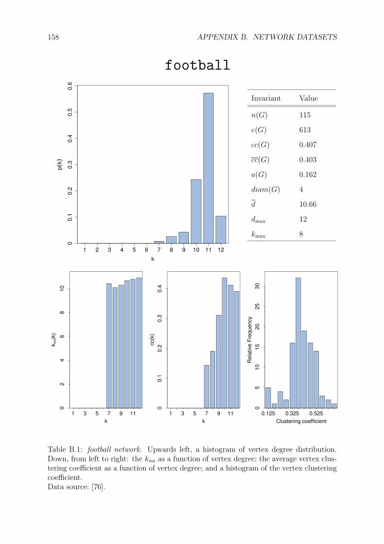
158 APPENDIX B. NETWORK DATASETS
football
k
p(k
)
1 2 3 4 5 6 7 8 9 10 11 12
00
.10
.20
.30
.40
.50
.6
Invariant Value
n(G) 115
e(G) 613
cc(G) 0.407
cc(G) 0.403
a(G) 0.162
diam(G) 4
d 10.66
dmax 12
kmax 8
k
kn
n(k
)
1 3 5 7 9 11
02
46
810
k
cc(k
)
1 3 5 7 9 11
00.1
0.2
0.3
0.4
Clustering coefficient
Rela
tive
Fre
quency
0.125 0.325 0.525
05
10
15
20
25
30
Table B.1: football network. Upwards left, a histogram of vertex degree distribution.Down, from left to right: the knn as a function of vertex degree; the average vertex clus-tering coefficient as a function of vertex degree; and a histogram of the vertex clusteringcoefficient.Data source: [76].

159
jazz bands
k
p(k
)
100
100.5
101
101.5
1021
0−
41
0−
31
0−
21
0−
11
00
p(k)
Invariant Value
n(G) 198
e(G) 2742
cc(G) 0.520
cc(G) 0.633
a(G) 0.020
diam(G) 6
d 27.70
dmax 100
kmax 29
k
k’
100
100.5
101
101.5
102
10
010
0.5
10
110
1.5
10
2
knn(k)
k
cc(k
)
100
100.5
101
101.5
102
10
−1
10
−0.5
10
0
cc(k)
Clustering coefficient
Rela
tive
Fre
quency
0.05 0.35 0.65 0.95
00.0
50.1
0.1
50.2
Table B.2: jazz bands network. Upwards left, a histogram of vertex degree distribution.Down, from left to right: the knn as a function of vertex degree; the average vertex clus-tering coefficient as a function of vertex degree; and a histogram of the vertex clusteringcoefficient.Data source: [78].

160 APPENDIX B. NETWORK DATASETS
Web (stanford.edu)
k
p(k
)
100
101
102
103
104
1051
0−
10
10
−8
10
−6
10
−4
10
−2
10
0
p(k)
f(k)=23.1k−2.28
Invariant Value
n(G) 255265
e(G) 1941926
cc(G) 0.009
cc(G) 0.653
a(G) −0.116
diam(G) 164(BCC)
d 15.21
dmax 38625
kmax 71
k
kn
n(k
)
100
101
102
103
104
10
010
110
210
310
4
knn(k)
f(k)=7089k−0.73
k
cc(k
)
100
101
102
103
104
10
−3
10
−2
10
−1
10
0
cc(k)
f(k)=12.28k−0.94
Clustering coefficient
Rela
tive F
requency
0.05 0.35 0.65 0.95
00.0
50.1
0.1
50.2
Table B.3: stanford.edu web network. Upwards left, a histogram of vertex degreedistribution, adjusted by max-likelihood for k ≥ 10. Down, from left to right: the knn asa function of vertex degree, adjusted to a power-law by least squares; the average vertexclustering coefficient as a function of vertex degree, adjusted to a power-law by leastsquares; and a histogram of the vertex clustering coefficient. Only the biggest connectedcomponent was considered (90.6% of the vertices).Data source: Stanford Large Network Dataset Collection http://snap.stanford.edu/
data/web-Stanford.html [103].

161
AS-CAIDA 2009
k
p(k
)
100
101
102
103
1041
0−
81
0−
61
0−
41
0−
21
00
p(k)
f(k)=0.512k−2.57
Invariant Value
n(G) 16117
e(G) 32847
cc(G) 0.013
cc(G) 0.472
a(G) −0.170
diam(G) 9
d 4.08
dmax 2012
kmax 16
k
kn
n(k
)
100
101
102
103
10
010
110
210
3
knn(k)
f(k)=630k−0.47
k
cc(k
)
100
101
102
103
10
−3
10
−2
10
−1
10
0
cc(k)
f(k)=1.2k−0.77
Clustering coefficient
Rela
tive
Fre
quency
0.05 0.35 0.65 0.95
00.0
50.1
0.1
5
Table B.4: AS-CAIDA 2009 network. Upwards left, a histogram of vertex degree distri-bution, adjusted by max-likelihood. Down, from left to right: the knn as a function ofvertex degree, adjusted to a power-law by least squares; the average vertex clusteringcoefficient as a function of vertex degree, adjusted to a power-law by least squares; anda histogram of the vertex clustering coefficient.Data source: The CAIDA UCSD IPv4 Routed /24 Topology Dataset - 2009-07-02, http://www.caida.org/data/active/ipv4_routed_24_topology_dataset.xml.

162 APPENDIX B. NETWORK DATASETS
AS-CAIDA 2011
k
p(k
)
100
101
102
103
1041
0−
81
0−
61
0−
41
0−
21
00
p(k)
f(k)=0.74k−2.48
Invariant Value
n(G) 19895
e(G) 44560
cc(G) 0.014
cc(G) 0.500
a(G) −0.170
diam(G) 9
d 4.48
dmax 2465
kmax 20
k
kn
n(k
)
100
101
102
103
10
010
110
210
3
knn(k)
f(k)=870k−0.48
k
cc(k
)
100
101
102
103
10
−3
10
−2
10
−1
10
0
cc(k)
f(k)=1.56k−0.77
Clustering coefficient
Rela
tive
Fre
quency
0.05 0.35 0.65 0.95
00.0
50.1
0.1
5
Table B.5: AS-CAIDA 2011 network. Upwards left, a histogram of vertex degree distri-bution, adjusted by max-likelihood. Down, from left to right: the knn as a function ofvertex degree, adjusted to a power-law by least squares; the average vertex clusteringcoefficient as a function of vertex degree, adjusted to a power-law by least squares; anda histogram of the vertex clustering coefficient.Data source: The CAIDA UCSD IPv4 Routed /24 Topology Dataset - 2011-06-30, http://www.caida.org/data/active/ipv4_routed_24_topology_dataset.xml.

163
AS-CAIDA 2013
k
p(k
)
100
101
102
103
1041
0−
81
0−
61
0−
41
0−
21
00
p(k)
f(k)=0.752k−2.53
Invariant Value
n(G) 23779
e(G) 54712
cc(G) 0.016
cc(G) 0.523
a(G) −0.171
diam(G) 9
d 4.61
dmax 2818
kmax 24
k
kn
n(k
)
100
101
102
103
10
010
110
210
3
knn(k)
f(k)=1148k−0.49
k
cc(k
)
100
101
102
103
10
−3
10
−2
10
−1
10
0
cc(k)
f(k)=1.84k−0.75
Clustering coefficient
Rela
tive
Fre
quency
0.05 0.35 0.65 0.95
00.0
50.1
0.1
5
Table B.6: AS-CAIDA 2013 network. Upwards left, a histogram of vertex degree distri-bution, adjusted by max-likelihood. Down, from left to right: the knn as a function ofvertex degree, adjusted to a power-law by least squares; the average vertex clusteringcoefficient as a function of vertex degree, adjusted to a power-law by least squares; anda histogram of the vertex clustering coefficient.Data source: The CAIDA UCSD IPv4 Routed /24 Topology Dataset - 2013-07-03, http://www.caida.org/data/active/ipv4_routed_24_topology_dataset.xml.

164 APPENDIX B. NETWORK DATASETS
AS-DIMES 2011
k
p(k
)
100
101
102
103
1041
0−
81
0−
61
0−
41
0−
21
00
p(k)
f(k)=0.637k−2.09
Invariant Value
n(G) 26083
e(G) 83305
cc(G) 0.015
cc(G) 0.643
a(G) −0.204
diam(G) 9
d 6.39
dmax 4517
kmax 35
k
kn
n(k
)
100
101
102
103
10
010
110
210
3
knn(k)
f(k)=2411k−0.53
k
cc(k
)
100
101
102
103
10
−3
10
−2
10
−1
10
0
cc(k)
f(k)=3.13k−0.78
Clustering coefficient
Rela
tive
Fre
quency
0.05 0.35 0.65 0.95
00.0
50.1
0.1
50.2
0.2
50.3
Table B.7: AS-DIMES 2011 network. Upwards left, a histogram of vertex degree distri-bution, adjusted by max-likelihood. Down, from left to right: the knn as a function ofvertex degree, adjusted to a power-law by least squares; the average vertex clusteringcoefficient as a function of vertex degree, adjusted to a power-law by least squares; anda histogram of the vertex clustering coefficient.Data source: DIMES, Distributed Internet MEasurements and Simulations, http://
www.netdimes.org/.

165
LiveJournal
k
p(k
)
100
101
102
103
104
1051
0−
12
10
−1
01
0−
81
0−
61
0−
41
0−
21
00
p(k)
f(k)=738.8x−2.58
Invariant Value
n(G) 4843953
e(G) 42845684
cc(G) 0.118
cc(G) 0.351
a(G) 0.021
diam(G) 16
d 17.69
dmax 20333
kmax 372
k
k’
100
101
102
103
104
10
010
110
210
310
4
knn(k)
k
cc(k
)
100
101
102
103
104
10
−4
10
−3
10
−2
10
−1
10
0
cc(k)
f(k)=35.98k−1.01
Clustering coefficient
Rela
tive F
requency
0.05 0.35 0.65 0.95
00.0
50.1
0.1
50.2
Table B.8: LiveJournal network. Upwards left, a histogram of vertex degree distribu-tion, adjusted by max-likelihood for k ≥ 50. Down, from left to right: the knn as afunction of vertex degree; the average vertex clustering coefficient as a function of vertexdegree, adjusted to a power-law by least squares; and a histogram of the vertex clus-tering coefficient. Only the biggest connected component was considered (99.9% of thevertices).Data source: Stanford Large Network Dataset Collection http://snap.stanford.edu/
data/soc-LiveJournal1.html [103].

166 APPENDIX B. NETWORK DATASETS
PGP
k
p(k
)
100
100.5
101
101.5
102
102.5
1031
0−
81
0−
61
0−
41
0−
21
00
p(k)
f(k)=0.88k−3.41
Invariant Value
n(G) 57243
e(G) 61837
cc(G) 0.403
cc(G) 0.504
a(G) 0.384
diam(G) 24 (BCC)
d 2.16
dmax 205
kmax 31
k
kn
n(k
)
100
100.5
101
101.5
102
10
010
0.5
10
110
1.5
10
2
knn(k)
f(k)=6.23k0.34
k
cc(k
)
100
100.5
101
101.5
102
10
−3
10
−2.5
10
−2
10
−1.5
10
−1
10
−0.5
10
0
cc(k)
f(k)=2.68k−0.66
Clustering coefficient
Rela
tive
Fre
quency
0.05 0.35 0.65 0.95
00.0
50.1
Table B.9: PGP trust network. Upwards left, a histogram of vertex degree distribution,adjusted by max-likelihood. Down, from left to right: the knn as a function of vertexdegree, adjusted to a power-law by least squares; the average vertex clustering coefficientas a function of vertex degree, adjusted to a power-law by least squares; and a histogramof the vertex clustering coefficient.Data source: [25].

167
E. Coli
k
p(k
)
100
100.5
101
101.5
102
102.5
1031
0−
61
0−
51
0−
41
0−
31
0−
21
0−
11
00
p(k)
f(k)=0.48k−1.68
Invariant Value
n(G) 1010
e(G) 3286
cc(G) 0.142
cc(G) 0.480
a(G) −0.106
diam(G) 10
d 6.51
dmax 143
kmax 9
k
kn
n(k
)
100
100.5
101
101.5
102
10
010
0.5
10
110
1.5
10
2
knn(k)
f(k)=20.83k−0.053
k
cc(k
)
100
100.5
101
101.5
102
10
−3
10
−2.5
10
−2
10
−1.5
10
−1
10
−0.5
10
0
cc(k)
f(k)=1.57k−0.72
Clustering coefficient
Rela
tive
Fre
quency
0.05 0.35 0.65 0.95
00.0
50.1
0.1
50.2
Table B.10: E. Coli metabolic network. Upwards left, a histogram of vertex degreedistribution, adjusted by max-likelihood. Down, from left to right: the knn as a functionof vertex degree, adjusted to a power-law by least squares; the average vertex clusteringcoefficient as a function of vertex degree, adjusted by least squares; and a histogram ofthe vertex clustering coefficient.Data source: [144].

168 APPENDIX B. NETWORK DATASETS

Bibliography
[1] R.D. Alba. A graph-theoretic definition of a sociometric clique. The Journal of
Mathematical Sociology, 3(1):113–126, 1973. 67
[2] R. Albert and A-L. Barabasi. Statistical mechanics of complex networks. Reviews
of Modern Physics, 74(1):47–97, January 2002. 45
[3] R. Albert, H. Jeong, and A-L. Barabasi. The diameter of the world wide web.
Nature, 401:130–131, 1999. 11, 17, 43, 147
[4] R. Albert, H. Jeong, and A-L. Barabasi. Error and attack tolerance of complex
networks. Nature, 406:200–0, 2000. 44
[5] J.I. Alvarez-Hamelin, M.G. Beiro, A. Barrat, L. Dall’Asta, and A. Vespignani.
Lanet-vi: Large network visualization tool. http://lanet-vi.fi.uba.ar/. 131,
135
[6] J.I. Alvarez-Hamelin, M.G. Beiro, and J.R. Busch. Understanding edge connectiv-
ity in the internet through core decomposition. Internet Mathematics, 7(1):45–66,
2011. 114, 125, 144
[7] J.I. Alvarez-Hamelin, L. Dall’Asta, A. Barrat, and Vespignani A. k-core decom-
position of internet graphs: hierarchies, self-similarity and measurement biases.
Networks and Heterogeneous Media, 3(2):371, 2008. 46, 114
[8] J.I. Alvarez-Hamelin, L. Dall’Asta, A. Barrat, and A. Vespignani. Large scale
networks fingerprinting and visualization using the k-core decomposition. In NIPS,
2005. 46
[9] J.I. Alvarez-Hamelin and N. Schabanel. An internet graph model based on trade-off
optimization. The European Physical Journal B - Condensed Matter and Complex
Systems, 38(2):231–237, 2004. 55
[10] A. Arenas, J. Duch, A. Fernandez, and S. Gomez. Size reduction of complex
networks preserving modularity. New Journal of Physics, 9(6):176, 2007. 71
169
170 BIBLIOGRAPHY
[11] D. Bailer-Jones. Scientific models in philosophy of science. University of Pittsburgh
Press Pittsburgh, Pa, 2009. 19
[12] P. Bak, K. Chen, and C. Tang. A forest-fire model and some thoughts on turbu-
lence. Physics Letters A, 147(5-6):297–300, 1990. 14, 17
[13] P. Bak, C. Tang, and K. Wiesenfeld. Self-organized criticality. an explanation of
1/f noise. Physical Review Letters, 59:381–384, 1987. 14, 17
[14] A-L. Barabasi and R. Albert. Emergence of scaling in random networks. Science,
286(5439):509–512, October 1999. 17, 43, 48, 53, 54
[15] A-L. Barabasi, R. Albert, and H. Jeong. Mean-field theory for scale-free random
networks. Physica A, 272:173–187, 1999. 54
[16] A. Barrat, M. Barthelemy, R. Pastor-Satorras, and A. Vespignani. The architecture
of complex weighted networks. Proceedings of the National Academy of Sciences,
101(11):3747, 2004. 33, 35
[17] A. Barrat and M. Weigt. On the properties of small-world network models. The Eu-
ropean Physical Journal B - Condensed Matter and Complex Systems, 13(3):547–
560, January 2000. 59
[18] V. Batagelj and M. Zaversnik. An o(m) algorithm for cores decomposition of
networks. arXiv, 2001. 39
[19] M.G. Beiro, J.R. Busch, and J.I. Alvarez-Hamelin. Snailvis: a paradigm to visual-
ize complex networks. In 39 Jornadas Argentinas de Informatica e Investigacion
Operativa (JAIIO), pages 1682–1693. SADIO, 2010. http://cnet.fi.uba.ar/
mariano.beiro/snailvis.tar.gz. 102, 110
[20] M.G. Beiro, J.R. Busch, S.P. Grynberg, and J.I. Alvarez-Hamelin. Obtaining
communities with a fitness growth process. Physica A: Statistical Mechanics and
its Applications, 392(9):2278 – 2293, 2013. 66, 143, 144
[21] E. A. Bender and E. R. Canfield. The asymptotic number of labeled graphs with
given degree sequences. Journal of Combinatorial Theory, Series A, 24(3):296–307,
May 1978. 48, 58
[22] G. Bianconi and A-L. Barabasi. Competition and multiscaling in evolving net-
works. Europhysics Letters, 54(4):436, 2001. 49

BIBLIOGRAPHY 171
[23] Y.M.M. Bishop, S.E. Fienberg, and P.W. Holland. Discrete Multivariate Analysis:
Theory and Practice. Springer, 2007. 36
[24] V.D. Blondel, J-L. Guillaume, R. Lambiotte, and E. Lefebvre. Fast unfolding
of communities in large networks. Journal of Statistical Mechanics: Theory and
Experiment, 2008(10):P10008, 2008. 71, 99
[25] M. Boguna, R. Pastor-Satorras, A. Dıaz-Guilera, and A. Arenas. Models of social
networks based on social distance attachment. Physical Review E, 70(5):056122+,
November 2004. 137, 166
[26] B. Bollobas. Graph Theory, An Introductory course. Springer-Verlag, New York,
Heidelberg, Berlin, 1979. 26
[27] B. Bollobas. Random Graphs. Cambridge University Press, 2001. 48
[28] B. Bollobas. Mathematical results on scale-free random graphs. In Handbook of
Graphs and Networks, pages 1–37. Wiley, 2003. 48, 54
[29] B. Bollobas and O. Riordan. The diameter of a scale-free random graph. Combi-
natorica, 24(1):5–34, January 2004. 54
[30] B. Bollobas, O. Riordan, J. Spencer, and G. Tusnady. The degree sequence of a
scale-free random graph process. Random Struct. Algorithms, 18(3):279–290, May
2001. 54
[31] U. Brandes, D. Delling, M. Gaertler, R. Gorke, M. Hoefer, Z. Nikoloski, and
D. Wagner. On modularity clustering. IEEE Transactions on Knowledge and
Data Engineering, 20(2):172–188, February 2008. 71, 84
[32] M. Bunge. Epistemologıa. Ariel, Barcelona, 1980. 7
[33] J.R. Busch, M.G. Beiro, and J.E. Alvarez-Hamelin. On weakly optimal partitions
in modular networks. CoRR, abs/1008.3443, 2010. 66, 84, 143
[34] CAIDA. The cooperative association for internet data analysis. http://www.
caida.org/. 46, 113
[35] G. Caldarelli and A. Vespignani. Large Scale Structure and Dynamics of Complex
Networks: From Information Technology to Finance and Natural Science. World
Scientific Publishing Co., Inc., River Edge, NJ, USA, 2007. 35, 42
[36] J. Carlson and J. Doyle. Highly optimized tolerance: A mechanism for power laws
in designed systems. Physical Review E, 60(2):1412–1427, 1999. 14, 17, 55

172 BIBLIOGRAPHY
[37] S. Carmi, S. Havlin, S. Kirkpatrick, Y. Shavitt, and E. Shir. Medusa - new model
of internet topology using k-shell decomposition. arXiv, January 2006. 46, 114
[38] S. Carmi, S. Havlin, S. Kirkpatrick, and E. Shir. A model of internet topology
using k-shell decomposition. PNAS, 104:11150–11154, 2007. 114
[39] M. Catanzaro, G. Caldarelli, and L. Pietronero. Assortative model for social net-
works. Physical Review E, 70(3), 2004. 49
[40] D.J. Chalmers. Strong and Weak Emergence, on The Re-Emergence of Emergence.
Oxford University Press, 2006. 6
[41] J. Chen and B. Yuan. Detecting functional modules in the yeast protein–protein
interaction network. Bioinformatics, 22(18):2283–2290, September 2006. 66
[42] F. Chung and L. Lu. The diameter of sparse random graphs. Advances in Applied
Mathematics, 26(4):257–279, May 2001. 50
[43] F.R.K. Chung and L. Lu. The average distance in a random graph with given
expected degrees. Internet Mathematics, 1(1):91–113, 2003. 48, 58
[44] A. Clauset, C. Moore, and M.E.J. Newman. Hierarchical structure and the pre-
diction of missing links in networks. Nature, 453(7191):98–101, 2008. 49
[45] A. Clauset, M.E.J. Newman, and C. Moore. Finding community structure in very
large networks. Physical Review E, 70(6):066111+, December 2004. 71, 74
[46] A. Clauset, C.R. Shalizi, and M.E.J. Newman. Power-law distributions in empirical
data. SIAM Review, 51(4):661–703, November 2009. 151, 155, 156
[47] J. Cohen. A coefficient of agreement for nominal scales. Educational and Psycho-
logical Measurement, 20(1):37, 1960. 36
[48] R. Cohen, K. Erez, D. ben Avraham, and S. Havlin. Breakdown of the internet
under intentional attack. Physical Review Letters, 86(16):3682–3685, April 2001.
44
[49] R. Cohen and S. Havlin. Scale-free networks are ultrasmall. Physical Review
Letters, 90(5):058701+, February 2003. 54
[50] P. Colomer de Simon, M.A. Serrano, M.G. Beiro, J.I. Alvarez-Hamelin, and
M. Boguna. Deciphering the global organization of clustering in real complex
networks. Scientific Reports, 3(2517), 2013. 135, 136, 137, 144

BIBLIOGRAPHY 173
[51] A. Condon and R.M. Karp. Algorithms for graph partitioning on the planted
partition model. Random Structures and Algorithms, 18(2):116–140, 2001. 49, 61
[52] T.M. Cover and J.A. Thomas. Elements of information theory. Wiley-Interscience,
New York, NY, USA, 1991. 76
[53] L. Danon, A. Dıaz-Guilera, and A. Arenas. Effect of size heterogeneity on com-
munity identification in complex networks. Journal of Statistical Mechanics,
2006(11):P11010, 2006. 71
[54] L. Danon, A.D. Guilera, J. Duch, and A. Arenas. Comparing community struc-
ture identification. Journal of Statistical Mechanics: Theory and Experiment,
2005(9):P09008–09008, September 2005. 75, 76
[55] D.J. De Solla Price. Networks of Scientific Papers. Science, 149(3683):510–515,
July 1965. 147
[56] DIMES. Distributed internet measurements and simulations. http://www.
netdimes.org/. 46, 113
[57] M.B. Doar. A better model for generating test networks. In Global Telecommuni-
cations Conference, 1996. GLOBECOM ’96. ’Communications: The Key to Global
Prosperity, pages 86–93, 1996. 48
[58] S. Dorogovtsev. Lectures on Complex Networks. Oxford University Press, Inc.,
New York, NY, USA, 2010. 42
[59] S.N. Dorogovtsev, A.V. Goltsev, and J.F.F. Mendes. Critical phenomena in com-
plex networks. Reviews of Modern Physics, 80:1275–1335, Oct 2008. 45
[60] S.N. Dorogovtsev, J.F.F. Mendes, and A.N. Samukhin. Structure of growing net-
works with preferential linking. Physical Review Letters, 85:4633–4636, 2000. 55
[61] J.C. Doyle, D.L. Alderson, L. Li, S. Low, M. Roughan, S. Shalunov, R. Tanaka,
and W. Willinger. The “robust-yet-fragile” nature of the internet. Proceedings of
the National Academy of Sciences, 102(41):14497–14502, October 2005. 44
[62] B. Drossel and F. Schwabl. Self-organized critical forest-fire model. Physical Review
Letters, 69:1629–1632, September 1992. 14
[63] J. Duch and A. Arenas. Community detection in complex networks using extremal
optimization. Physical Review E, 72:027104, 2005. 71

174 BIBLIOGRAPHY
[64] P. Erdos and A. Renyi. On random graphs i. Publicationes Mathematicae Debrecen,
6:290, 1959. 48, 49
[65] A. Fabrikant, E. Koutsoupias, and C.H. Papadimitriou. Heuristically optimized
trade-offs: A new paradigm for power laws in the internet. In Proceedings of the
29th International Colloquium on Automata, Languages and Programming, ICALP
’02, pages 110–122. Springer-Verlag, 2002. 17, 48, 55
[66] M. Faloutsos, P. Faloutsos, and C. Faloutsos. On power-law relationships of the
internet topology. In Proceedings of the conference on Applications, technologies,
architectures, and protocols for computer communication, SIGCOMM ’99, pages
251–262, New York, NY, USA, 1999. ACM. 17, 43, 53, 113
[67] R.A. Fiesner. Advances in Chemical Physics, Computational Methods for Protein
Folding. Wiley-Interscience, 2001. 9
[68] G.W. Flake, S. Lawrence, and C.L. Giles. Efficient identification of web com-
munities. In Proceedings of the sixth ACM SIGKDD international conference on
Knowledge discovery and data mining, KDD ’00, pages 150–160, New York, NY,
USA, 2000. ACM. 65, 67, 70
[69] L.R. Ford and D.R. Fulkerson. Maximal flow through a network. Canadian Journal
of Mathematics, 8:399–404, 1956. 30
[70] S. Fortunato. Community detection in graphs. Physics Reports, 486(3-5):75 – 174,
2010. 69, 77
[71] S. Fortunato and M. Barthelemy. Resolution limit in community detection. Pro-
ceedings of the National Academy of Sciences, 104(1):36–41, January 2007. 81
[72] L.C. Freeman. A set of measures of centrality based on betweenness. Sociometry,
40(1):35–41, March 1977. 37
[73] L.C. Freeman. Centrality in social networks: conceptual clarification. Social Net-
works, 1(3):215–239, 1979. 37
[74] R. Garcia. Sistemas complejos. Conceptos, metodo y fundamentacion episte-
mologica de la investigacion interdisciplinaria. Gedisa, Barcelona, 2006. 7
[75] M. Gardner. Mathematical games: The fantastic combinations of john conway’s
new solitaire game “life”. Scientific American, pages 120–123, 1970. 6, 17

BIBLIOGRAPHY 175
[76] M. Girvan and M.E.J. Newman. Community structure in social and biological
networks. Proceedings of the National Academy of Sciences, 99(12):7821–7826,
June 2002. 37, 61, 69, 100, 158
[77] J.P. Gleeson. Bond percolation on a class of clustered random networks. Physical
Review E, 80(3):036107+, September 2009. 136, 137
[78] P. Gleiser and L. Danon. Community structure in jazz. Advances in Complex
Systems, 6(4):565–573, July 2003. 72, 100, 159
[79] T. Gneiting and M. Schlather. Stochastic models that separate fractal dimension
and the hurst effect. SIAM Review, 46(2):pp. 269–282, 2004. 21
[80] R.E. Gomory and T.C. Hu. Multi-terminal network flows. Journal of the Society
for Industrial and Applied Mathematics, 9(4):551–570, 1961. 127, 128
[81] B.H. Good, Y.A. De Montjoye, and A. Clauset. Performance of modularity maxi-
mization in practical contexts. Physical Review E, 81(4):046106, 2010. 84, 99
[82] R. Govindan and A. Reddy. An analysis of internet inter-domain topology and
route stability. In Proceedings of the INFOCOM ’97. Sixteenth Annual Joint Con-
ference of the IEEE Computer and Communications Societies. Driving the In-
formation Revolution, INFOCOM ’97, pages 850–, Washington, DC, USA, 1997.
IEEE Computer Society. 113
[83] R. Govindan and H. Tangmunarunkit. Heuristics for internet map discovery. In
Proceedings of the INFOCOM 2000. Nineteenth Annual Joint Conference of the
IEEE Computer and Communications Societies, pages 1371–1380, Washington,
DC, USA, 2000. IEEE Computer Society. 113
[84] C.W.J. Granger and Roselyne Joyeux. An introduction to long-memory time series
models and fractional differencing. Journal of Time Series Analysis, 1(1):15–29,
1980. 21
[85] R. Guimera and L.A.N. Amaral. Cartography of complex networks: modules and
universal roles. J. Stat. Mech.-Theory and Exp., 2:02001+, February 2005. 71
[86] R. Guimera and L.A.N. Amaral. Functional cartography of complex metabolic
networks. Nature, 433(7028):895–900, February 2005. 66
[87] R. Guimera, L. Danon, Dıaz A. Guilera, F. Giralt, and A. Arenas. Self-similar
community structure in organisations. Physical Review E, 68, 2002. 72
176 BIBLIOGRAPHY
[88] B. Gutenberg and C. Richter. Frequency of Earthquakes in California. Bulletin of
the Seismological Society of America. Seismological Society of America, 1944. 147
[89] F. A. Hayek. Degrees of explanation. The British Journal for the Philosophy of
Science, 6(23):pp. 209–225, 1955. 19
[90] H. Jeong, B. Tombor, R. Albert, Z.N. Oltval, and A-L. Barabasi. The large-scale
organization of metabolic networks. Nature, 407:651–654, October 2000. 44, 45
[91] S. Johnson, J.J. Torres, J. Marro, and Miguel A. Munoz. Entropic origin of disas-
sortativity in complex networks. Physical Review Letters, 104(10):108702+, March
2010. 47
[92] J. Kleinberg. Navigation in a small world. Nature, 406:845, 2000. 49
[93] P. L. Krapivsky, S. Redner, and F. Leyvraz. Connectivity of growing random
networks. Physical Review Letters, 85:4629–4632, November 2000. 54
[94] A.E. Krause, K.A. Frank, D.M. Mason, R.E. Ulanowicz, and W.W. Taylor. Com-
partments revealed in food-web structure. Nature, 426(6964):282–285, November
2003. 66
[95] J.M. Kumpula, J. Saramaki, K. Kaski, and J. Kertesz. Limited resolution in
complex network community detection with potts model approach. The European
Physical Journal B, 56(1):41–45, 2007. 79, 81, 82, 83
[96] A. Lancichinetti, S. Fortunato, and J. Kertesz. Detecting the overlapping and
hierarchical community structure in complex networks. New Journal of Physics,
11(3):033015, 2009. 72, 73, 84, 85, 86
[97] A. Lancichinetti, S. Fortunato, and F. Radicchi. Benchmark graphs for testing
community detection algorithms. Physical Review E, 78(4):046110, October 2008.
49, 61, 73
[98] E.L. Lawler. Cutsets and partitions of hypergraphs. Networks, 3(3):275–285, 1973.
67, 70
[99] E.A. Leicht and M.E.J. Newman. Community structure in directed networks.
Physical Review Letters, 100(11):118703+, March 2008. 71
[100] W.E. Leland, M.S. Taqqu, Willinger W., and D.V. Wilson. On the self-similar
nature of ethernet traffic. In In Proceedings of the ACM SIGCOMM’93, 1993. 17,
21
BIBLIOGRAPHY 177
[101] J. Leskovec and E. Horvitz. Planetary-scale views on a large instant-messaging
network. In Proceedings of the 17th international conference on World Wide Web,
WWW ’08, pages 915–924. ACM, 2008. 10
[102] J. Leskovec, J. Kleinberg, and C. Faloutsos. Graphs over time: densification laws,
shrinking diameters and possible explanations. In Proceedings of the eleventh ACM
SIGKDD international conference on Knowledge discovery and data mining, KDD
’05, pages 177–187, New York, NY, USA, 2005. ACM. 49
[103] J. Leskovec, K.J. Lang, A. Dasgupta, and M.W. Mahoney. Community structure in
large networks: Natural cluster sizes and the absence of large well-defined clusters.
Internet Mathematics, 6(1):29–123, 2009. 100, 160, 165
[104] C. Levinthal. How to Fold Graciously. In J. T. P. Debrunnder and E. Munck,
editors, Mossbauer Spectroscopy in Biological Systems: Proceedings of a meeting
held at Allerton House, Monticello, Illinois, pages 22–24. University of Illinois
Press, 1969. 8
[105] N. Litvak and R. van der Hofstad. Degree-degree correlations in random graphs
with heavy-tailed degrees, October 2012. 47
[106] R.D. Luce and A.D. Perry. A method of matrix analysis of group structure. Psy-
chometrika, 14(2):95–116, 1949. 67
[107] T. Luczak. Size and connectivity of the k-core of a random graph. Discrete Math-
ematics, 91(1):61 – 68, 1991. 46
[108] D. C. Mikulecky. The emergence of complexity: science coming of age or science
growing old? Computers and Chemistry, 25(4):341–348, 2001. 3
[109] R.J. Mokken. Cliques, clubs and clans. Quality & Quantity, 13(2):161–173, April
1979. 67
[110] E. Morin. La Methode I. La nature de la nature. Seuil, 1977. 7
[111] M.E.J. Newman. The structure of scientific collaboration networks. Proceedings
of the National Academy of Sciences, 98(2):404–409, January 2001. 65, 67
[112] M.E.J. Newman. Assortative mixing in networks. Physical Review Letters,
89:208701, October 2002. 35
[113] M.E.J. Newman. Fast algorithm for detecting community structure in networks.
Physical Review E, 69, September 2003. 72, 77

178 BIBLIOGRAPHY
[114] M.E.J. Newman. Mixing patterns in networks. Physical Review E, 67(2), 2003.
36, 45, 46
[115] M.E.J. Newman. The structure and function of complex networks. SIAM Review,
45:167–256, 2003. 42, 153
[116] M.E.J. Newman. Power laws, pareto distributions and zipf’s law. Contemporary
Physics, 46(5):323–351, May 2005. 147, 151, 155
[117] M.E.J. Newman. Finding community structure in networks using the eigenvectors
of matrices. Physical review E, 74(3), 2006. 71, 78
[118] M.E.J. Newman. Random Graphs with Clustering. Physical Review Letters,
103(5):058701+, July 2009. 136
[119] M.E.J. Newman. Networks: An Introduction. Oxford University Press, Inc., New
York, NY, USA, 2010. 37
[120] M.E.J. Newman and M. Girvan. Finding and evaluating community structure in
networks. Physical Review E, 69(026113), 2004. 70
[121] A. Noack and R. Rotta. Multi-level algorithms for modularity clustering. In
Proceedings of the 8th International Symposium on Experimental Algorithms, SEA
’09, pages 257–268, Berlin, Heidelberg, 2009. Springer-Verlag. 71
[122] L. Page. Method for node ranking in a linked database. United States patent
6,285,999, 2001. 46
[123] G. Palla, I. Derenyi, I. Farkas, and T. Vicsek. Uncovering the overlapping commu-
nity structure of complex networks in nature and society. Nature, 435(7043):814–
818, June 2005. 72, 73
[124] J-J. Pansiot and D. Grad. On routes and multicast trees in the internet. Computer
Communication Review, 28(1):41–50, January 1998. 113, 114
[125] R. Pastor-Satorras, A. Vazquez, and A. Vespignani. Dynamical and correlation
properties of the internet. Physical Review Letters, 87:258701+, 2001. 35, 46, 114
[126] R. Pastor-Satorras and A. Vespignani. Epidemic spreading in scale-free networks.
Physical Review Letters, 86(14):3200–3203, April 2001. 45, 112
[127] J. Plesnık. Critical graphs of a given diameter. Acta Facultatis Rerum Naturalium
Universitatis Comenianae: Mathematica, 30:71–93, 1975. 123

BIBLIOGRAPHY 179
[128] D.D. Price. A general theory of bibliometric and other cumulative advantage
processes. Journal of the American Society for Information Science, 27(5):292–
306, 1976. 43, 54
[129] F. Radicchi, C. Castellano, F. Cecconi, V. Loreto, and D. Parisi. Defining and iden-
tifying communities in networks. Proceedings of the National Academy of Sciences,
101(9):2658, 2004. 69, 85
[130] U.N. Raghavan, R. Albert, and S. Kumara. Near linear time algorithm to detect
community structures in large-scale networks. Physical Review E, 76(3):036106+,
September 2007. 72, 99
[131] E. Ravasz and A-L. Barabasi. Hierarchical organization in complex networks.
Physical Review E, 67(2):026112, February 2003. 47
[132] J. Reichardt and S. Bornholdt. Statistical mechanics of community detection.
Physical Review E, 74(1):016110, July 2006. 78, 83
[133] H. Reittu and I. Norros. On the power-law random graph model of massive data
networks. Perform. Eval., 55(1-2):3–23, January 2004. 58
[134] L. G. Rodrıguez Zoya and J.L. Aguirre. Teorıas de la complejidad y ciencias
sociales; nuevas estrategias epistemologicas y metodologicas. Nomadas. Revista
Crıtica de Ciencias Sociales y Jurıdicas, 30(2), 2011. 7
[135] R. Rosen. Life Itself: A Comprehensive Inquiry into the Nature, Origin, and
Fabrication of Life (Complexity in Ecological Systems). Columbia University Press,
July 2005. 6, 19
[136] A. Rosenblueth and N. Wiener. The role of models in science. Philosophy of
Science, 12(4):pp. 316–321, 1945. 19
[137] M. Rosvall, D. Axelsson, and C.T. Bergstrom. The map equation. The European
Physical Journal Special Topics, 178(1):13–23, 2009. 73
[138] M. Rosvall and C.T. Bergstrom. An information-theoretic framework for resolving
community structure in complex networks. Proceedings of the National Academy
of Sciences, 104(18):7327–7331, 2007. 73, 74, 98
[139] M. Rosvall and C.T. Bergstrom. Maps of random walks on complex networks
reveal community structure. Proceedings of the National Academy of Sciences,
105(4):1118–1123, 2008. 73

180 BIBLIOGRAPHY
[140] K. Saito, T. Yamada, and K. Kazama. Extracting communities from complex net-
works by the k-dense method. IEICE Transactions on Fundamentals of Electronics
Communications and Computer Sciences, E91-A(11):3304–3311, November 2008.
39, 137
[141] S.B. Seidman. Network structure and minimum degree. Social Networks, 5(3):269
– 287, 1983. 39
[142] S.B. Seidman and B.L. Foster. A graph-theoretic generalization of the clique con-
cept. Journal of Mathematical Sociology, 6:139–154, 1978. 67
[143] E. Seneta. Non-Negative Matrices and Markov Chains. Springer, 2006. 38
[144] M.A. Serrano, M. Boguna, and F. Sagues. Uncovering the hidden geometry behind
metabolic networks. Molecular BioSystems, 8:843–850, 2012. 137, 167
[145] G. Siganos, S.L. Tauro, and M. Faloutsos. Jellyfish: A conceptual model for the as
internet topology. Journal of Communications and Networks, 8(3):339–350, 2006.
114
[146] S. Smyth and S. White. A spectral clustering approach to finding communities in
graphs. Proceedings of the 5th SIAM International Conference on Data Mining,
pages 76–84, 2005. 78
[147] C. Song, S. Havlin, and H.A. Makse. Self-similarity of complex networks. Nature,
433(7024):392–395, January 2005. 47
[148] G. Tibely and J. Kertesz. On the equivalence of the label propagation method of
community detection and a potts model approach. Physica A: Statistical Mechanics
and its Applications, 387(19-20):4982–4984, 2008. 72
[149] J. Travers and S. Milgram. An experimental study of the small world problem.
Sociometry, 32:425–443, 1969. 9, 17
[150] Route Views. University of oregon route views project. http://www.routeviews.
org/. 46, 113
[151] K. Wakita and T. Tsurumi. Finding community structure in mega-scale social
networks. In Proceedings of the 16th international conference on World Wide Web,
WWW ’07, pages 1275–1276, New York, NY, USA, 2007. ACM. 71
[152] D.J. Watts. Small worlds: The dynamics of networks between order and random-
ness. Princeton University Press, Princeton, NJ, 1999. 49

BIBLIOGRAPHY 181
[153] D.J Watts and S.H. Strogatz. Collective dynamics of small-world networks. Nature,
393:440–442, 1998. 12, 17, 33, 48, 59
[154] B.M. Waxman. Routing of multipoint connections. IEEE Journal on Selected
Areas in Communications, 6(9):1617–1622, 1988. 48, 51
[155] W. Weaver. Science and complexity. American Scientist, 36(4):536–544, 1948. 3,
4, 5, 16
[156] D.B. West. Introduction to Graph Theory (2nd Edition). Prentice Hall, 2000. 26,
30, 31, 32, 41
[157] S. Wolfram. A New Kind of Science. Wolfram Media, 2002. 13
[158] W. Y. Yang and M. Gruebele. Folding at the speed limit. Nature, 423:193–197,
2003. 8
[159] S.H. Yook, F. Radicchi, and H. Meyer-Ortmanns. Self-similar scale-free networks
and disassortativity. Physical Review E, 72(4):045105, 2005. 47
[160] W. Zachary. An information flow model for conflict and fission in small groups.
Journal of Anthropological Research, 33:452–473, 1977. 10
[161] E.W. Zegura, K.L. Calvert, and M.J. Donahoo. A quantitative comparison of
graph-based models for internet topology. IEEE/ACM Transactions on Network-
ing, 5(6):770–783, December 1997. 48

182 BIBLIOGRAPHY

Index
Asch’s experiment, 9
assortativity, 36, 47
by degree, 35
austrian school, 16
Autonomous System, 111
behavior
assortative, 36, 46, 47
disassortative, 36, 46, 47, 49
betweenness, 37
binning, 149
logarithmic, 150
cellular automaton, 6, 12
centrality, 36
chaotic system, 4
closeness, 37
clustering coefficient, 33, 135
collective behavior, 6
community
in a strong sense, 69
in a weak sense, 69, 85
natural, 72, 85, 86
web, 67
community structure, 46, 49
complex system
adaptive, 17
definition, 7
complex systems models, 18
agent-based, 6, 17, 18
cellular automata, 6, 12, 21
differential equation, 20
mean-field, 20
recurrence equation, 20
time series, 14, 20
connectivity, 32, 112
cover, 72, 85
cybernetics, 16
diameter, 33
distribution
heavy-tailed, 12, 156
scale-free, 12, 44, 153
edge-betweenness, 69
edge-connectivity, 32, 115
strict sense, 123
wide sense, 123
eigenvector centrality, 38, 46
emergence, 5
emergentism, 6
strong, 6
weak, 6
feedback, 16, 45
fitness function, 72, 84, 85
fractal theory, 12, 17
fraction of correctly classified vertices, 77
game of life, 6, 12, 17
graph
definition, 26
random, 47
growth process, 85
uniform, 91
183

184 INDEX
highly optimized tolerance (HOT), 14, 17,
55, 112
histogram, 149
holism, 6
hypergraph, 137
Jaccard index, 76
k-core, 39
k-dense, 39, 137
k-shell, 124
linear regression, 151
long-range dependency, 14, 21
maxima verosimilitud, 151
Milgram’s experiment, 9, 43
minimum description length, 73
mixing patterns, 36, 46
model
Barabasi-Albert (BA), 17, 53
configuration, 58
definition, 19
Erdos-Renyi, 49
FKP, 17, 55
forest-fire, 14, 17
LFR, 61, 74
planted l-partition, 61, 74
sandpile, 14, 17
Watts-Strogatz, 12, 17, 59
Waxman’s, 51
modularity, 70
mutual information, 75
normalized, 76
network
CAIDA, 130, 131, 161–163
complex, 18, 22
DIMES, 130, 131, 164
E. Coli metabolic, 137, 167
football, 78, 94, 158
jazz bands, 100, 159
karate (Zachary), 10, 19
LiveJournal, 101, 165
metabolic, 65
PGP trust, 137, 166
protein interaction, 43, 66
trophic, 66
Web (Barabasi), 11, 43
Web (Stanford), 100, 108, 160
power-law, 12, 14, 15, 43
preferential attachment, 17, 48, 53
protein folding, 7
scientific reductionism, 6
self-organized criticality (SOC), 14, 17
self-similarity, 14
small-world, 9, 12, 43, 135
system, 7