c l a s p snuffler: geophysics software from sussex university

Doc. Ref: TR08CLASP TrainingInstruction Manual for ‘Snuffler’ Software Iss./Date: A, Dec. 13

C L A S P

Snuffler: Geophysics Software from Sussex University:Introduction and Help File

After coming across a cheap resistivity meter provided by the 'Council for Independent Archaeology'and 'TR Systems Ltd' I decided to try writing some Windows software to go with it. The software isnot restricted to this particular meter however, and can be used for any resistivity or magnetometrydataset in electronic or paper format, and most importantly it is FREE.

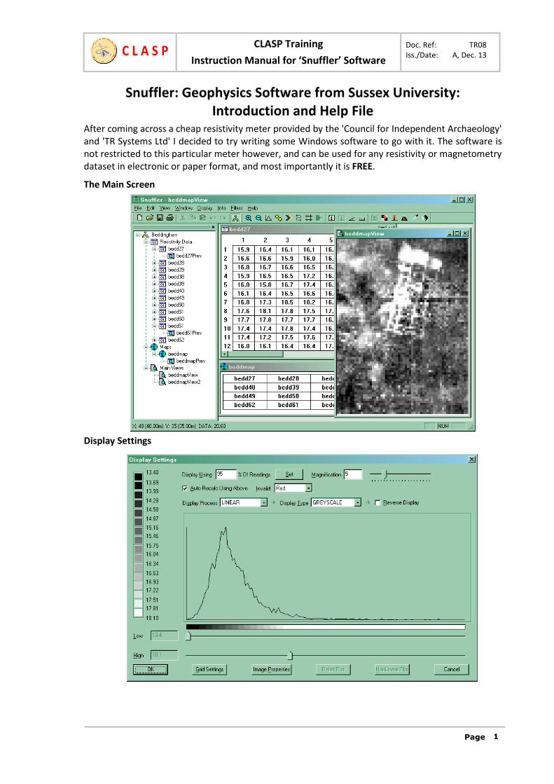
The Main Screen

Display Settings


C L A S P

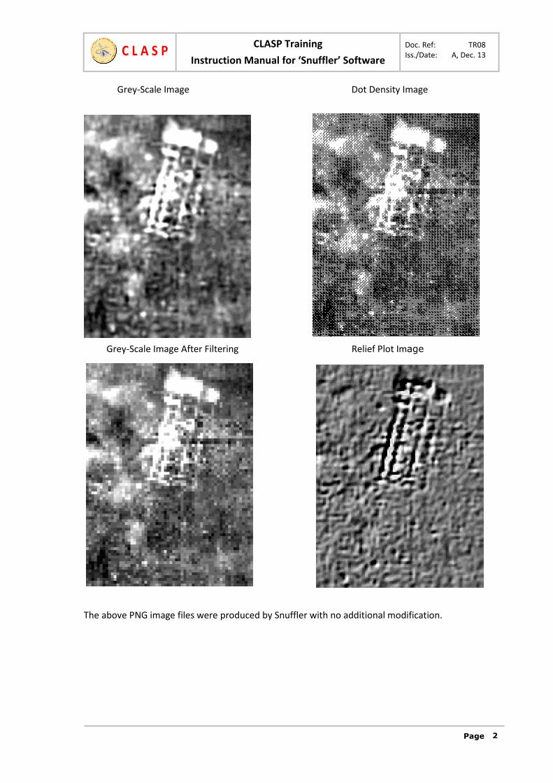
Grey-Scale Image Dot Density Image

Grey-Scale Image After Filtering Relief Plot Image

The above PNG image files were produced by Snuffler with no additional modification.


C L A S P

Features: Enter data from keyboard or text files Import from RM15 & TR Systems resistivity meters, FM18/36 magnetometers, Arc-Geo

logger, Bartington GRAD601 and EPE Resistivity Meter Export data to text files Preview data sets Image view in Grey Scale, Dot Density and Relief Display range clipping Data and selection statistics Print images with image info Export images to PNG (Portable Network Graphic) image files and VRML Metadata Storage Continuously sampled data processing Filters, including:

Despike Direct modification of data in a selection Interpolation Geological Flattening Sharpen Edge correction Destripe Clip Data Destagger


C L A S P

Snuffler Help file

1. Main Help PageWelcome to Snuffler, a Freeware geophysics program designed for Archaeological Resistivity andMagnetometry. Actually this is not Freeware, it is Hugware. If after 30 days of use, you decide tocontinue using the software, you must find someone you love and give them a big hug. If you arenot feeling in a mood for hugs, but think the author deserves some reward for writing this, thenthere is a donate button on the website.

The version you are running is Beta software (v0.90), it is undergoing testing prior to a full releaseand is in no way polished, bug-free or stable. As this software is still in development, I would verymuch appreciate if you let me know of any bugs you come across or features you would like to see.

In addition to problems with the software, I would also like to know about problems with this helpfile. As I have written this software, everything about it seems obvious to me, yet it may seemobtuse to everyone else. So please let me know if I have not explained something properly, orindeed if I have not explained it at all.

1.1 Getting StartedIf you are reading this, you have already successfully installed the software. Snuffler will create itselfa directory in your documents folder, but if you want to change this, you can do so in the OptionsMenu.

Once you have set the software up to your satisfaction, please read the File Overview section. If youdon't know much about the basic processes involved in geophysics, check out the ResistivityRefresher. Once you understand how the program works, there is some Sample Data for you to playaround with.

1.2 Resistivity RefresherThis section is for those who don't know the basics of Resistivity. Resistivity is a type ofArchaeological Prospecting that works by measuring the 'Resistivity' of the ground in a grid of pointsacross a site.

The process itself works like this. A section of ground to be 'measured' has a set of probes pushedinto the surface, which pass an electrical current through the ground. As electricity conducts wellthrough water, the amount of water in the soil will affect how much resistance there is to thecurrent being passed through it. If there is little moisture, the electricity meets greater resistance inpassing through the soil, which is said to have a high resistance value. If there is a lot of moisture inthe ground, the current passes through it easily and is said to have low resistance. A numerical valuerepresenting exactly how much resistance is met is calculated by the resistivity meter. Given a set ofsuch measurements in a regular pattern across a site, a picture can be created, which is where thissoftware comes in.

What does this have to do with archaeology?

The amount of moisture in the soil can be affected by a range of underground archaeologicalfeatures. For example, if there is a pit cut into the bedrock, this pit may have a greater capacity forstoring moisture than the surrounding rock, so the topsoil above will dry out slower as there is asupply of stored moisture, which will give a low resistance reading. Alternatively, if you have thefoundations of a brick wall underneath the topsoil, there is less room for stored moisture and thetopsoil dries out quicker, giving a high resistance reading. Many other factors can affect this, such as


C L A S P

soil type and density, but without getting into the nitty gritty, just remember that it is thedifferences in resistance across a site that we are interested in, as these show up as recognisablepatterns on the images produced by this software.

1.3 Sample Data SetIncluded with the other files in this software is a sample data set of a Roman Villa in XYZ format. Thefilename is testdata.txt and can be found in the same directory that the software was installed. Dotake the time to look at the file yourself to see what the raw data looks like. To use this yourself,start by creating a blank Project by selecting 'New Project' from the file menu and choosing a newname for the project.

Now you will need to import the file into Snuffler. You can do this by going to the file menu andselecting Easy XYZ Import Into New File. You will be prompted for a filename, at which point, youwill need to find the directory on your computer where the software is installed, and locate thetestdata.txt file. The software will look at the file and bring up the screen with some options, whichyou can ignore for the moment. Just Press OK and the file will be read. You now have a file full ofdata. These files are described in greater detail in the Geophysics Data Files section of this help file.

Now comes the part where we create an image from the data file. For this you will need to use theProject Window on the left hand side of your display. This lists all of the files currently in the projectyou are working on in what is known as a tree display. This tree has branches that can be expandedand collapsed. To the left of each icon in this display is either a + or - sign in a small box. Clicking onthis will expand or collapse that branch of the tree. So if you click now on that box, you should nowsee another branch called 'Geophysics Data' which contains all of your data files. Clicking on the boxnext to this branch should show you the data file you have created. Right clicking on the icons (notthe boxes) in the Project Window will bring up a submenu. You now want to do this with your datafile. Right-clicking on the icon will bring up a sub-menu, from which you want to select 'Spawn MainView'. This will add another branch to the tree and create a basic image for you to see. Theseimages are described in the View Files section of this documentation.

2. User Interface

2.1 MenusThe Menus at the top of the Snuffler window will change according to which type of file you haveopen at the time, giving access to functions appropriate to that file. Nevertheless, there are menuoptions that are available with whatever type of file you are editing. For other menu options, seethe help pages specific to the different file types.

File Menu

Some menu options are available even when you don't have a project open: New Project Creates a new, empty, project Open Project Opens an existing project Print Setup Sets how your images will appear when Printing Options Sets options controlling the behaviour of the software

Other menu options in the file menu are only available with a project open: Save Project Save current project. This only affects the Project Options, as all other files

are saved separately Close Project Close the currently open project New Create new Geophysics Data, Preview, View, Map or Import file


C L A S P

Open Open an existing file within the project Project Options Sets the Options for the current project only (these are copied initially

from the main options when the project is created). Project Metadata Store various pieces of information about the current project Easy XYZ Import Allows you to read in an XYZ file

View Menu

Allows you to hide or show the Toolbar, the Status Bar (at the bottom of the screen, and the ProjectBar. The help menu allows you to see this file!

Toolbar

The Toolbar at the top of the Snuffler window is a useful shortcut for performing a lot of tasks:

The three icons in the File section represent New, Open, Save and Print, which act the sameas the functions on the File Menu.

The five icons in the Edit section represent Cut, Copy, Paste, Undo and Redo from the EditMenu. The first three are detailed in the page on View Files. Undo is used to put back achange that you have made to an image if you don't like it. Redo undoes the Undo.

The Toggle Project Bar button turns the Project Bar on and off, in the same way as theProject Bar option in the View Menu.

The two magnify icons can be used to increase and decrease magnification of the displayedimage without going into the Display Settings. These two icons are only available in thePreview and View windows.

In the Display section of the toolbar, there are eight buttons, which are only available in thePreview and View windows. The first two increase and decrease magnification, the nextbutton brings up the main Display Settings window. The next two change the displayprocess and display type respectively. The sixth, Reverse Display, will reverse the palette ifyou are using a linear process, but will move the horizontal angle on 45 degrees if you areusing the Relief plot process. The seventh will activate or deactivate the Display Gridaround the grid squares of your image. Finally, the last button will set the display clippingbounds to the high and low values within the area you have selected.

The Info section of the toolbar contains four buttons which perform exactly the same tasksas the options within the info menu.

The Filters section of the toolbar contains nine buttons, which are only available whenworking in a View. They are (in order) the filters, Modify Selection, Interpolate, RemoveSpikes, Remove Geology, Sharpen, Edge Correction, Destripe, Clip Data and Destagger.

As well as using the Toolbar, many functions can be accessed using Keyboard Shortcuts.

Keyboard Shortcuts

As well as the menus and the Toolbar, many of the functions in Snuffler can be controlled by thekeyboard. Following is a list of keys used in Snuffler.

Ctrl+N New Document Ctrl+O Open Document Ctrl+P Print Document Ctrl+Alt+P Print Preview Ctrl+S Save Document Alt+Backspace Undo Ctrl+Backspace Redo


C L A S P

F1 Help F6 Next Document Alt+P Toggle Project Window Ctrl+Shift+P Set the focus to the project bar

The following keys are used in Main Views and Previews only : Alt+C Set Clip To Selection Alt+D Display Settings Alt+G Toggle Grid Alt+R Reverse Display Alt+T Next Display Type Alt+N Next Process Type Ctrl+A Select All Ctrl+C Copy Ctrl+X Cut Ctrl+V Paste Ctrl+Shift+V Transparent Paste Ctrl+Alt+V Paste As New View Ctrl+R Rotate Clockwise Shift Holding this down whilst selecting or pasting will align to grid square edges Ctrl Holding this down whilst selecting will align to lines within grid squares

2.2 ProjectsProjects And File Overview

To use Snuffler, you will need to know about the different types of files it uses. PROJECT FILES: The first thing you will need to do is create a project. A 'project'

encompasses all of the data you will need for a site you are surveying. The details of theproject and the various data files within it are displayed in the Project Window on the leftside of your screen. To create a project, select 'New Project' from the file menu. You will beprompted to enter a name for the project. When this is done, Snuffler will create theproject and allow you to create the other types of files listed below, which form part of theproject.

IMPORT DATA FILES: An Import Data File is the file containing the raw data imported fromyour resistivity meter, which is just a string of numbers. The next stage in the importprocess is to export to individual data files, or grids, from which an image can be compiled.

Geophysics DATA FILES: A Geophysics Data File contains readings for a single grid square.The default size for these squares is 20x20, but can be changed to whatever size you want.The readings can be keyed into the file manually, read in from a text file or importeddirectly from whatever geophysics equipment you are using via an import file.

MAP FILES: A Map File types holds information on the location of the above data files inrelation to eachother. Composite images can then be generated from this map.

PREVIEW FILES: A Preview is a graphical display of a set of data. Either of an individual gridsquare or of a composite image generated from a map. As the preview is linked directly tothe data, it changes as the data changes. Also, this means that no filters or other changescan be made to the preview, as this would affect the original data it is generated from.Preview files are not necessary for the process of creating an image, they are designed soyou can see the image changing as you type in data from the keyboard, to make the processless boring.

VIEW FILES: A View File is similar to a preview file, except once it has been created, it isindependent from the data it was created from. This means that changes to the original


C L A S P

data will not affect it, and changes, such as filtering, can be applied to the view itself. This isthe main file used for viewing the results created from your data.

As well as files used directly by Snuffler, there are other file formats used independently by Snuffler,that it can import or export.

PNG FILES: PNG (Portable Network Graphics) is the graphics file format that Snufflerexports. It is used as opposed to other file formats because it is unencumbered by patents,is lossless, and is well supported. For more information on this file format see the officialwebsite at http://www.libpng.org/pub/png/

XYZ FILES: XYZ files are text files formatted in a certain way that contain data with alocation. Snuffler can both import and export XYZ files. The name of the file format refers tothe position of the data (X & Y), and the data itself (Z), and this is how that data is arrangedon each line of the file: eg, if the X position is 20 metres, Y position 25.5 metres and the datais 45.67, the XYZ file reads “20.0 25.5 45.67”.

RES2DINV FILES: RES2DINV is a software package that produces resistance tomographyimages, that is using resistance to take a vertical slice through the ground. The processinvolved in doing this, called Inversion, is quite complex, so Snuffler simply provides anexport in the appropriate format for RES2DINV to read. This export was originally designedwith the TR Systems tomography setup in mind, but should work with data from any meterthat can produce the data in the same way. The data is exported on a per grid basis, fromthe data files, and those files must be in a certain order to export correctly. The size of thegrid should be the number of probes used by the number of lines. Dummy readings arealways put in at the end of lines, never at the beginning. The first line should have threedummy readings at the end, with each subsequent line having three less again. Contrary tothe instructions given in the TR Systems documentation, you do not need to go back to thebeginning of the line each time. You can zig-zag if you wish, you just need to tell Snufflerthat you have done so when creating the grid from the import file. Thus if you do not zig-zag, all the dummy readings will be at one end of the grid, but if you do zig-zag, the dummyreadings will alternate between each end between lines.

2.3 Project WindowThe Project Window is the large white bar on the left side of your screen when Snuffler starts up.When a project is created or loaded, details of the files contained within the project are shown inthis window. The files are arranged in what isknown as a tree, the nodes of which can beopened and closed using the +/- icons on thetree, just like in Windows Explorer. The projectitself is shown at the top with the name of theproject next to an icon consisting of a bluediamond surrounded by three yellow boxes.The same icon on the Toolbar will make theProject Window appear and disappear ifpressed. An example of how the project barmay look is shown below. The project windowcan be made to float by double-clicking on thebar at the top of the window, and can beresized by dragging the right side of thewindow.

Below the project itself in the project windowis a list of the files in the project that expands


C L A S P

as new files are created. New files can be added to the project either using the 'new' menu option inthe 'file' menu, or the new file button, which is the first button on the toolbar at the top of theSnuffler window.

Once files have been created, they can be opened (if not already so) by simply double clicking withthe left mouse button on the relevant icon in the tree. A menu of functions that relate to these filescan also be accessed by right clicking on the icon. Three menu options which are common to all filetypes are Open, which acts in the same way as double-clicking on the file, Delete, which will deletethe file from the list, destroying it forever without any hope of return (you have been warned), andRename, which allows you to change the name of the file.

Additionally, the following types of files will have additional functions available on their pop-upmenu.

Geophysics Data Files You can also use the Preview Window option to create a graphicalPreview for your grid square and create a View File incorporating the single data file usingthe Spawn Main View option. They also have an Export Data submenu, which allows theraw data contained within the file to be exported to a text file in the order selected, an XYZfile, or a RES2DINV file if the data is in the correct format for a pseudo section. For this lastoption, you will be asked to confirm the order in which the data was taken.

Map Files also have the same Preview Window option as the Data Files above, and can alsocreate a View Window using the Spawn Main View option and save the map as an easilyviewed text file using the Export Map As Text File option.

Import Files can't be deleted, for your own good, but they do have an 'Export To Text File'option to allow you to dump the raw data into a text file, and 'Create Data Grids', which willallow you to split the raw imported data into individual grid squares.

In addition to these, you can access the Project Options and Project MetaData by right-clicking onthe project entry in the project window. New files can also be created by right-clicking on the filegroup headings.

2.4 Project MetaDataProject MetaData means data about the project. It is here that you store the various pieces ofinformation that would normally be in a notebook or on the back of an envelope. While it is notessential, it is good practise to store this information for those people who didn't actually take partin the survey and may not be able to get this type of data any other way. Thanks to the irritatingobtuseness of human memory, you will undoubtedly find it useful yourself in many years to come,no offence intended :)

The MetaData screen is accessible either by using the Project MetaData... option in the File Menu,or by right clicking on the Project Name in the Project Window. The Project MetaData window isdivided into three subsections, which can be accessed using the tabs at the top. They are Survey,which relates to the nature of the survey and what is intended to be accomplished, Geographical,which relates to the location and geology of the area under survey, and finally, Instrument, whichrelates to the hardware used, and its configuration.

In the Survey section, the following entries are available: Survey Dates: The dates over which the survey was carried Weather: The weather at time of survey. Rain is especially relevant to Resistivity Monument Type: What you are expecting to find or have found. e.g. Villa, Causewayed

Enclosure Monument period: The chronological period(s) of the monuments found Surveyor: The individuals/organisations involved in performing the survey Comments: Any other comments on reasons for survey / interpretation of results.


C L A S P

In the Geographical section, the following entries are available: Survey Name: Full name of survey, e.g. Ditchling Beacon Resistivity Survey 2001 Reference: If you have any relevant internal or external references for this survey, store

them here Map Coordinates: The grid references for the limits of the survey Country: The country in which the survey took place Administrative Area: The country/parish in which the survey took place Solid Geology: Underlying solid geology under survey area, e.g. Chalk, Limestone Drift Geology: Temporal Geology, e.g. Alluvium, Colluvium, Dunes Soil Condition: Information on condition of soil due to weather/geology/agriculture Land Use: What the land has historically been used for

In the Instrument section, the following entries are available: Instrument Type: e.g. Resistivity meter, magnetometer Instrument Make/Model: Who made it, and the model number Instrument Configuration: e.g. Twin Probe, Wenner, Schlumberger Transverse Separation: Distance between the lines transversed within the grid Reading Interval: How far between each reading along the line of survey Magnetic North: Clockwise offset between magnetic north and the top of the survey grid,

needed for magnetometer surveys

2.5 Options and project optionsIn the 'File' menu are two items marked Options and Project Options. When selected, a window willappear with a set of preferences to change the behaviour of the software. Though they bothcontain the same preferences, the difference between the two is that 'Options' contains items thatare set in the project when it is created. These can then be changed for a single project using the'Project Options' menu item.

The options are divided into two sections. Those on the left are general options relating to thesoftware, the options on the right relate to the setup of individual pieces of hardware.

The general options on the left are as follows:


C L A S P

Default Data Directory: the directory to which Snuffler writes its files. For the 'Options', thisis the main directory in which the project subdirectories are created. In the 'ProjectOptions', this is the name of the subdirectory for this project, which cannot be changed. Ifyou want to change the location of a project on your hard disk, simply move the filessomewhere else. NB: the project considers any files that are in its directory as part of thatproject, so don't get them mixed up.

Default Magnification: the magnification level that images start on when first created. Readings Per Metre: also defaulted when you are asked for the dimensions of a new set of

geophysics data. Default Invalid Colour: the default colour used in images where there is no data to display. Import Valid Range: the range, outside which imported data is marked as invalid. Decimal Places For Data: the number of decimal places (zero, one or two) used for storing

geophysics data.The hardware-specific options are on the right. You can select the Default Import Hardware, whichis the machine first shown when you start an import. If you have a favourite piece of hardware, thenset this so you don't need to change it when doing an import each time.

If you change the Default Settings For options, the rest of the right hand area will display theoptions specific to that piece of hardware. Those options are as follows.

Default Grid Size: the width and height defaulted when you are asked for the dimensions ofa new set of geophysics data.

Readings Per Metre: relates to the default grids as above. Zero Point Drift: defaults for the Fm18/FM36 whether or not this option is active Com Port: the default com port that the machine is plugged into Baud Rate: the default speed of transfer from the machine Import Valid Range: the range of readings, outside which the data will be marked as a

dummy reading

2.6 File types

2.6.1 Import filesUnless you are importing your data from some sort of file, or keying it in by hand, the first steptowards producing an image is to import the data from your geophysics meter. At the moment,Snuffler supports downloading from the following :

Geoscan Research RM15 TR/CIA Resistivity Meter Geoscan Research FM18/36 Arc-Geo Logger Bartington GRAD601 EPE Resistivity Meter

Please note, the download from these meters is entirely unofficial. The companies that produce thehardware are in no way responsible for the download features available in this software. Havingsaid that, if you wish your meter to be supported by Snuffler, then just pop one in the post, and I'llsort it out for you :)

To start reading in data from your meter, the first thing to do, is create an import file, which can bedone from File > New > Import File or by clicking the New button on the toolbar and selecting DataImport.


C L A S P

You will then be asked for several pieces of information. First of all, the name of the import file youwish to create should be entered in Import Name, which must not be the same as any otherfilename already created. There is also a choice of Hardware, i.e. RM15, TR, FM18/36, Arc-Geo,GRAD601, EPE. You also need to say which Comms Port that your meter is attached to, and theBaud Rate used, all of which is defaulted from the Project Options.

Next you have to tell Snuffler how much data you want to read, and there are three ways of doingthis. If in the Import Quantity box you have selected Grids, then you can enter two more values.The Quantity in this case is the number of complete grids you wish to download, and the StartPosition is the grid you wish to start at. For the TR Systems meter, the GRAD601 and the EPE meter,the grid information is downloaded with the data. For the RM15 and FM18/36, you have to specifyit yourself by entering the Grid Settings, which is dictated by the settings in the Project Options. TheArc-Geo is similar to the RM15, though you do not download the grids all at once. You can set animport for multiple grids and then you have to set the Arc-Geo to download each grid, whichSnuffler will collect in a single import file. The EPE meter data consists of a single 128x128 grid,which is downloaded in its entirety each time.

If you have an RM15, you also have the option of importing a number of readings rather than grids.You do this by selecting Readings in the Import Quantity box, then entering the appropriatenumbers in the Quantity and Start boxes. The third option, All, is only available on the TR Systemsmeter and the GRAD601 because the RM15 and FM36 do not stop sending data when it reaches theend! This option will read all the grids in the memory of the meter.

At this point, you can also split into grids, rather than waiting until later. First select Split Into GridsNow, then enter the prefix which you want to use for the data grid filenames. If you do decide tosplit the data into grids now, you will be asked for the order in which the readings will be taken after


C L A S P

the download has completed. If you are using a magnetomer, such as an FM18 or FM36 and havelogged drift readings, you should tick the Zero Point Drift box to make sure this is processedcorrectly.

After you have made your selections, there are separate procedures to start the download. RM15/FM18/FM36: With any Geoscan meter, you then need to press the OK button on the

Meter Import window. A small window will appear that will show you how many readingshave been downloaded, which will read zero until you start the download. You can pressStop at any time to abort the process. Snuffler is now waiting for data to be sent from themeter, so start the download process on your meter, which with an RM15 is started bypressing the DUMP button on the meter itself, and Snuffler will read the data until it hasread as many as you have asked for, at which point the read process will automatically stop,and you can press the Cancel button on your meter to stop the process, and turn the meteroff.

TR Systems: With the TR systems meter, you first need to turn the meter on and press theDOWNLOAD button on the meter itself. This will not start sending the data as with theRM15, but allows the computer itself to activate the download process. You can now pressthe OK button on the Snuffler 'Meter Import Window', which will tell the meter to startdownloading, displaying the number of readings in the same manner as the RM15. Whenthe process has finished, you can turn the meter off.

Arc-Geo Logger: For the Arc-Geo Logger, you must follow these steps after you haveentered the correct details. Firstly, set the AUTO/MANUAL switch in the AUTO position onthe logger and then set the bank and grid switches to choose which grid to download. Pressthe OK button on the Snuffler 'Meter Import Window' then press D/LOAD followed byYES/LOG on the logger.

GRAD601: Turn on the meter and arrow down to select the Output Data option on themeter. The meter will then wait until you press the OK button on the Snuffler 'Meter ImportWindow', which will tell the meter to start transmitting. Once the download is complete,turn the meter off.

EPE Resistivity Meter: Turn on the meter. Press the OK button on the Snuffler 'MeterImport Window', followed by the Download button on the meter. Once the download iscomplete, turn the meter off.

You now have a file containing the imported data, and the next stage, if you have not already doneso by entering the appropriate information into the grid split box, is to split this up into individualgrids, and there are two ways of doing this. The quickest and easiest way is to right click on theimport file in the Project Window and select Create Data Grids. You will first be prompted to enter afile name prefix. Snuffler will create grids beginning with this name, also followed by the nextavailable number in a sequence beginning at one (unless you are exporting a single grid). Secondly,you will be prompted to enter the order in which the readings were taken. For the TR meter, thiswill default to that shown in the manual, though you are not limited to this. Snuffler will then createa set of Data Files. For the RM15, which does not store grid information for download, the grid sizedictated by the settings in the Project Options. The downside of this method is that all the gridshave to be the same size with the same readings order. For the TR Systems meter, the grid sizes arestored for download, so you can have different grid sizes created from an import file. For the EPEmeter, you are not asked for the order in which the readings progress, as the order is kept withinthe meter itself.

A more flexible but much slower method is to create individual grids yourself and import data a gridat a time by right clicking within the Data File window itself and selecting Import Data > FromImport File from the menu that appears. The size is then dictated by the size of the grid you havecreated, and the data order can be changed for each grid you do.


C L A S P

2.6.2 Geophysics Data FilesA Geophysics Data File contains the raw data produced by the geophysics equipment you are using.Each file represents a single grid square. To create a geophysics data file in your project, selectGeophysics Data File from the 'file' menu and within it the 'New' menu. You will be asked for aname for the grid square, which must be unique in your project. A common prefix followed by anumber for the grid is a good name to use. You will also be asked to specify the size of the gridsquare, which defaults to 20x20 (or whatever is specified in the Project Options) and also thenumber of readings per metre, which will be important later on.

When the file has been created, it will in the project on the left hand side of the Snuffler window, aswell as showing the empty grid on the right. Now you have this empty grid, you can start to enteryour data into it. There are several ways of doing this. First of all, points for which there are no datacan be marked by simply double-clicking in them with the left mouse button, which will mark it withan X. Part of a completed grid is shown below.

If you want to edit the value of a single point in the grid, click within it with the right mouse buttonand select 'Edit Cell' from the menu that appears. You will be asked to enter the value for this point,after which you press enter or click ok to save it. You can also mark the point as having no data byclicking in the invalid box or using the ALT-I key combination, which acts in the same way as if youdouble-clicked within the point with the left mouse button, to mark it with an X. You will see thatthe data you are entering is to one decimal place. If you are working with two, or zero, you canchange this in the Project Options.

This is of course a very slow way to enter in your data. If you don't have the benefit of reading inyour data from a file, there is still a quicker way to enter inyour data from the keyboard. If you right click anywherewithin the grid square and then select 'Import Data > FromKeyboard', you can enter in the data without having to selectevery single point.

First of all, you will be presented with a box asking you inwhich order you are entering the data. You can select whichcorner you are starting from as well as whether you are to gohorizontally or vertically. Finally, you can select whether youwant to double-back when you get to the end of the line youare keying, or go back to the start of the line, with the 'Bi-Directional' tick box.

Once you have chosen the order in which you are keying, youwill be presented with the same data entry box as you sawwhen changing the data in a single point. The difference hereis when you have entered your data, the box will appear again


C L A S P

asking for the next point along, until you stop it, or thegrid is full. Another feature that is activated in thismode that is not available when editing a single cell, isthe ability to enter multiple invalid values with a singlekeypress. The count shown under 'Fill with' is defaultedto the number of cells that are left in the line you arekeying, so you can just use ALT-V or click on the 'InvalidValues' button to fill the rest of the line with invalidvalues. You can of course change the value to enter adifferent number of invalid values.

The ideal way to enter data into Snuffler is from a text file. Snuffler treats any number, '.' or '-' asnumerical data, separated by anything that doesn't fall into this category. The exception to this is 'X'or 'x' which is treated as a point with no data. To read in from a file. Click the right mouse button inyour grid and select 'Import Data > From Text File' from the menu. You will be asked for the order inwhich to import the data, in the same manner as importing from the keyboard above. Snuffler willthen check that the number of data items found in the file matches the number of empty pointswithin the grid. If it matches, the file will be read into the grid. If invalid points are represented inthe file by something other than an 'x', or not represented at all, the invalid sections of the grid canbe selected first using the left mouse button, as detailed above. Remember, the software will readyour text file in sequential order and enter those values into the Grid in the order that you specify. Ifyou want to see how this works, try entering data from the keyboard to see how you progressaround the grid as you enter values. With this type of file import, and the other two listed below,there is a threshold of what is considered valid data. Outside of this, the data is marked as invalid.The default range is from -3000 to 3000, though this can be changed in Options and Project Options.

Another type of text file is called an XYZ file,which has on each line, the x position, the yposition and the data, one line for eachpiece of data. Snuffler can read these files,but you must first make sure your data gridis the correct size, and most importantly,empty. To use this feature, use the menuoption 'Import Data > From XYZ File'. Afterselecting the file you want to import, youwill be presented with the window shownon the left. The first option, 0,0 Origin isuseful for software compatibility. Thoughthe XYZ format has absolute positioning ofdata, not all software agrees on where 0,0is. For example, Geoplot and Snuffler have0,0 in the Top-Left, whilst Surfer and theTR-Systems software have it in the Bottom-Left. Chosing the right option now will saveflipping your data later on. The secondoption allows you to select what you wantas a dummy (invalid) value. Any non-numeric value in the Z column of the data will be entered asinvalid, and the Non-Numeric Only option will leave it as just that. Geoplot uses 2047.5 as a dummyvalue, so select that if you are importing a file produced by Geoplot. If you want Zero as the invalidnumber then there is an option for that, or you can enter a value under Other Dummy Value to useas invalid data. Finally, All Of The Below, the default, means any of those options will produce aninvalid value. Please note that whilst this software can read XYZ files with X & Y values that are not


C L A S P

whole numbers, it cannot yet cope with continuous sampling data where the number of data pointalong a line is not the same as the number of lines. You can also export Text, XYZ and RES2DINV filesusing the 'Export Data' submenu, in the same way as the menu options in the Project Window.Further information on these file types can be found in the Projecta And File Overview

Another way to import data is from a Geoplot file. These files have an extension of 'DAT' for a singlegrid, and 'CMP' for a composite, and sometimes come with an associated file with an extension of'CMD', which describes the data. You still have to set up the grid first and tell it how big it is, but thewidth and height can be found in the CMD file, which is a simple text file that can be viewed withnotepad. Geoplot seems to represents invalid data with the number 2047.5. Since the Geoplot filesare always in the same order, you will not be asked to specify which order to read in the data.Otherwise, the import process is much the same as for a text file.

As well as creating several grids at once from an Import File, you can copy data from one of theseinto a data file using the 'Import Data > From Import File'. The advantage of this is all of theimported grids don't have to be of the same size or survey direction. You just select the start grid orreading you want and the survey direction, and the data will be imported.

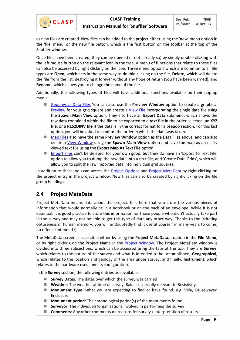
A final feature to take note of is veryuseful when keying in data manually. Youcan select blocks of readings by holdingdown the left mouse button anddragging the mouse. The selected areawill be highlighted in red and can bemanipulated using three menu optionsavailable on the context menu when youright click.They are all under the sub-menu 'Change Selected Cells', whichcontains 'Delete Cell Contents', whichwill clear the selected area of any data,'Set Cells To Invalid' which will set all the readings in the area to invalid, and 'Shift Cells', which willmove the readings in the selected area. This is especially useful if you are keying data and you havemissed out a reading or a line. Rather than delete everything and start again, the mis-aligned datacan be shifted to its correct position and the missing data entered in the correct place. Please note,shifted data will overwrite any data that it is shifted over. There is no undo, so be careful. Inaddition to these three options, the selected area will also be affected by the standard 'Cut', 'Copy'and 'Paste' from the 'Edit' menu.

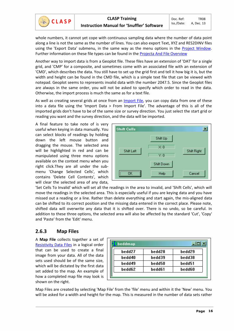
2.6.3 Map FilesA Map File collects together a set ofResistivity Data Files in a logical orderthat can be used to create a finalimage from your data. All of the datasets used should be of the same size,which will be dictated by the first dataset added to the map. An example ofhow a completed map file may look isshown on the right.

Map Files are created by selecting 'Map File' from the 'file' menu and within it the 'New' menu. Youwill be asked for a width and height for the map. This is measured in the number of data sets rather


C L A S P

than metres. Once you have entered this data, you will be presented with a blank grid. There aretwo ways to fill in the map grid.

If you left-click within one of the squares of this grid, you will be presented with a list ofavailable datasets. The dataset name will appear in the grid when selected.

A quicker way to select grids for inclusion in the map is using the right mouse button. Thisfeature assumes all of the data grids in the project use the same prefix, followed by anumber. E.G. 'griddat1', 'griddat2', 'graddat3'. If you click in the map with the right mousebutton, Snuffler will take the data grid with the lowest unused number and put it in themap. So the first time you click, Snuffler will use 'griddat1' and the second time, it will use'griddat2', etc. This will not work if there is already data in the grid or there is more thanone prefix in the data sets of the project.

If you have an existing map and have surveyed more of the area around it, rather than just creatinga new map and selecting all the grids you have already entered, you can resize the map by using theEdit -> Resize Map menu option.

When you have filled the grid, or as much of it as is needed, you can then create a Preview or Viewfile from it using the Project Window. The preview is not necessary, to creating the final image. TheView itself, which you will be able modify using Filters can be created by right clicking on the map inthe Project Window and selecting Spawn Main View.

Map Files can be saved as an easily readable text file by right clicking on the map in question in theProject Window and selecting Export Map As Text File.

2.6.4 Preview FilesA Preview File is one of two display files, the other being the View File. The difference between thetwo is that a Preview File is directly linked to the data (either a Data File or Map File) that itrepresents, so as you update the data, the Preview is also updated to reflect the changes. The ViewFile on the other hand, is independent of the data it was created from.

The use of preview windows is not necessary in the process of creating an image. It was included inthis program so when you are typing in data using the keyboard, you can see the image beinggenerated as you type, which makes the process a little less boring. If you are not interested in this,just use View Files

To create a Preview Window for a data set or map, right click on your chosen item in the ProjectWindow and select 'Preview Window' from the menu that appears. You can only create one previewfor each data set or map. You will be asked for a name for the preview, which defaults to the nameof the map file plus the word 'Prev'. Another way to create a Preview for a set of data is to use theNew menu option in the file menu or the New File icon on the Toolbar. You will then be asked fromwhich data set to create a preview for.

What you see in the preview window is a graphical display of your numerical data. You can't applyFilters to the Preview Window, but you can change the Display Settings and use the info menu.

As in a View File, the Copy option from the edit menu is activated in a Preview Window, though notthe cut and paste options as the data cannot be changed.

2.6.5 View FilesA View File is similar to a Preview File, except that instead of the data being read from the file it islinked to, a View File holds its own set of data and is not dependant on the data it was created from.Because of this independence, Filters can be used to change the view data. This View File is the


C L A S P

main place where you display and modify your results, Preview Files are not necessary in theprocess of generating a final image.

View Files can be created from Map Files and Resistivity Data Files, though a blank view can also becreated using the New option from the File Menu or the New File icon on the Toolbar. In the lattercase, you will be asked to give a size for the newly created view. This view is blank but can be editedto fill it with data using the Cut/Copy/Paste option explained below. As with Preview Files, Viewfiles are created using the Project Window. Clicking with the right mouse button on the map or dataof your choice will bring up a menu, from which you should select 'Spawn Main View'. You will beasked for a name for the view, which defaults to the name of the map/data file plus the word'View'.

As with the Preview Files, you can change the Display Settings, but you can also use Filters to modifythe View.

The Cust/Copy/Paste options in the Edit Menu and on the Toolbar can all be used on Views, to copya section of an image to the clipboard, drag the mouse with left button down to select the area youwant to copy, then just use the copy menu option, icon or Ctrl+C to copy to the clipboard. Cut(Ctrl+X) acts in much the same way, except it blanks the area you have copied to the clipboard. ToPaste the contents of the clipboard to the View, select Paste (or use Ctrl+V). You will notice themouse pointer has changed, and it is at this point that you select a point in the view with the leftmouse button to place the top-left corner of where you want the data pasted. The paste operationcan be cancelled with the right mouse button. Another useful feature when using paste is that afteryou have selected the paste option, you can hold down the shift key when selecting where to pasteto, and the software will place your data against the top-left hand corner of the grid square youhave clicked in. There are two additional Paste options in the Edit Menu. Transparent Paste(Ctrl+Shift+V) is the same as the normal Paste, except any area that does not contain valid data willnot be copied. This is useful when you are copying an area with an irregular outline and therectangle you are pasting would otherwise overwrite an area containing data with blank data. PasteTo New View (Ctrl+Alt+V) takes the contents of the clipboard and pastes it into a new view, whichyou are prompted for a name.

It should also be noted that copying or cutting an image will place a copy of that image on thewindows clipboard. Unfortunately, this is currently limited to what you can see on the screen at thetime, but this will hopefully be rectified in a future release.

Also in the Edit Menu, are three options, which will Flip Horizontal, Flip Vertical and Rotate 90 DegClockwise and Rotate 180 Degrees. Useful if you realise you have the image the wrong way up.These will also work on selected areas if they encompass entire grids, but the rotate 90 function willnot operate if the grid size and pitch are not the same.

If you right click within an open View File image, a small menu will appear with the followingoptions. Display Settings, Image Information and Selection Information act the same as in theFilters Menu

In the File menu, you will also have access to an Export submenu, which has the following options: To Text File: This option will export the data to a text file, with one reading on each line.

You will be asked in what order you wish to export the data. To XYZ File: This option will export the data as an XYZ file, which is a standard data file

recognised by many pieces of geophysics software. Each line stores the position of the data(X & Y) and the data itself (Z).

To VRML: A VRML file is a file which contains 3D data, and the value of the readings in thefile are taken as the height. These files can be viewed by browser with a suitable plugin.


C L A S P

PNG File: Whilst the first three files export the data underlying the image, this option willexport the image itself. The PNG file format is a popular open file format replacement forGIF, and is considered most suitable for archive purposes.

Finally, a note on selecting parts of your image, which also applies to Preview Files. Severalfunctions in the program require you to select part of your image to work. This is done by movingthe mouse pointer to one corner of the area you want to select, holding down the left mousebutton and dragging the mouse to the opposite corner. The area you have selected will behighlighted and any function which requires an area to be selected will be activated. The selectioncan be de-selected by clicking at a single point on the image without moving the mouse. There areother means of selecting parts of the image. By pressing CTRL+A, you will select the entire image. Byholding down the Shift key, and selecting an area, as you normally would, you will select entire gridsquares that the mouse pointer passes through. By holding down the Ctrl key, and selecting an area,as you normally would, you will select lines within grid squares that the mouse pointer passesthrough. The extent of the selection you have made will be shown in the status bar at the bottom ofthe Snuffler window.

2.7 Display SettingsThe Display Settings window controls how an image is displayed can be accessed from the Previewand View windows by right clicking with the mouse and selecting 'Display Settings', or in the case ofthe View window, you can also select it from the display menu at the top of the screen or using therelevant icon on the toolbar. Below is an example of what the Display Settings window may looklike.

The main focus of this window, and the first part we will learn about is the clipping. Clipping iswhere you set an upper and lower value to display, so anything outside of these bounds will bedisplayed just as the highest or lowest value. The reason for doing this, is if you use the full range of


C L A S P

readings to display with just the 16 shades available, you will have very large blocks of readingsdisplayed using the same colour, which is not very helpful for interpretation. By clipping the displayof the image, we can reduce the range of values represented by a single shade.

In the middle of the display settings window you will see a graph representing the values in thedata. The horizontal axis of the graph measures resistance in ohms whilst the vertical axis measuresthe number of readings with this resistance. The purpose of this graph is to help you decide the highand low bounds you want for clipping. For an average set of data, you will see something like a bellcurve displayed on the graph. Below the graph are two sliding bars with numbers next to themwhich represent the low and high values used for the clipping. You will find that you will not be ableto change these. This is because the computer is handling the clipping itself.

The automatic clipping system is represented by two controls above the left hand side of the graphand are called 'Display Using ***% Of Readings' and 'Auto Recalc Using Above'. The latter tickboxturns the auto clipping on and off, it is on by default. If you turn it off, you can manually set theclipping bounds using the two sliders below the graph. When it is on, the computer will take thepercentage value shown in the first control, and that percentage of the readings closest to theaverage as within the clipping bounds. If you change this percentage, the computer will recalculatethe clipping bounds using the new percentage. This automatic clipping applies to changes made tothe data itself. Say you apply a Filter to the image. When it is done, the computer will recalculatethe clipping bounds automatically. Whether the bounds are decided by yourself or by the computer,the high and low values for each shade in the scale will be displayed to the left of the graph.

For magnetometer data, which has a range of values that goes into the negative, a tickbox isactivated called 'Centre on Zero' that will centre the automatic clipping on Zero. This is beneficial forthe de-stripe filter, and is activated for magnetometer data by default, but if you do not wish it todo this, you can turn off this feature by un-ticking the box.

Moving on from clipping, some of the other controls should be explained. 'Invalid' is the colour usedfor invalid areas of data, you can choose from Red, Yellow, Green, Blue, Black and White. The'Magnification' slider and value control how small or large the resulting image is. 'Info On Screen'displays the extra information associated with a printout, such as the scales, on the screen, so theycan be outputted in PNG files. 'Display Process' controls how the software processes the data toproduce a display. At the moment, this can either be 'LINEAR' which is the standard process bywhich a range of values are assigned to a specific colour on the output, and 'RELIEF PLOT', wherethe data is taken as height values and an artificial light is shone to produce areas of light and dark,or 'NONLINEAR' where there is still a simple scale like the linear plot, but the colour boundaries arenot all equal. This process is explained further down this page. 'Display Type' is how the data isdisplayed once processed, and is a collection of palletes of colour or greyscale, which are explainedbelow. The 'Reverse Display' flag will flip the scale, so that low readings come out light and highreadings come out dark. Many of these functions can also be controlled by buttons on the Toolbar.

GREYSCALE is the standard means of viewing an image. It is made up of 16 shades of grey and anyresulting images exported to a PNG file are browser safe. DOT DENSITY is not as nice on the eyes,but is useful when printing out to a black and white printer that cannot handle. RELIEF PLOT createsa '3D' illuminated image, described further below. EXT GREYSCALE, or more fully, EXTENDEDGREYSCALE, is like the normal greyscale except there are 31 rather than 16 shades of grey. This isuseful when you have a heavily interpolated image where you want smooth shading. RGB,EXT RGBand RAINBOW can be used if you want something more colourful with more contrast.


C L A S P

The 'Relief Plot' button brings up awindow that controls the displaycharacteristics of the Relief Plot. This is adisplay mode that treats the image as a3D object, with the high resistancereadings being treated as a high pointand the low resistance readings as a lowpoint. A virtual light source is shone onthis object, which will be lit accordingly.The origin of this light source can becontrolled from the Relief Plot Window,in which you can change the horizontal(0-359 degrees) and vertical (0-90degrees) angles from which the lightsource shines. The relief plot is good for showing up features in geologically noisy areas as it showschanges in readings relative to the adjacent readings rather than relative to the image as a whole. Agood vertical angle to use is 40 degrees, whilst the horizontal angle can be quickly selected using thesmall squares around the horizontal angle indicator. Features can easily appear and disappeardepending on which horizontal angle you use, so try a few. It should also be noted that a betterresult can be achieved in a lot of cases if you use the interpolate filter first before trying the ReliefPlot. You will also notice a 'False-Relief' tickbox. If you select this, the rest of the options for therelief plot will be turned off. The purpose of this is not to shine a light from a specific direction, buthave the hue generated dependant of the contrast of the readings with their immediateneighbours. Whilst this works as a process, the results are not particularly helpful, so this is left as afeature of limited interest, just to show that it can be done.

The 'Nonlinear Plot' encompasses severalprocesses under one banner. What theyhave in common is they still assign coloursto a range of readings like the linear plot,but the ranges each colour are assigned toare not equal. When you select Nonlinear asa process, a button marked 'NonLinear Plot'will become active at the bottom of theDisplay settings window. Clicking this willbring up the window shown on the left. Asyou can see, there are four sub-processesthat you can select. The default process 'UseData Distribution' is probably the mostuseful. Whereas the linear plot will assignblocks of colour to equal ranges of valueswithin the clipping bounds, this process willassign the colours to equal numbers ofreadings, so the colour bands are quite wideat the edges of your clipping area wherethere are few readings, but narrow near thecentre, where most of your readings will beclustered. This has the effect of increasingthe contrast in your image. You will notice atthe bottom of the window a 'Severity' bar.This is not active for the Data Distribution


C L A S P

option, as the process does not support it, but the other three options do. These options highlightparticular blocks of readings by narrowing the range for a colour in the area you wish to higlight.The 'Highlight Middle' option will produce similar results to the data distribution option, as theshape used to generate the colour boundaries is similar to the shape of the average distributioncurve. The severity slider at the bottom can be used to increase or decrease the effect produced.The 'Highlight Low' and 'Highlight High' also assign the colours based on a shape, but in this case atthe lower and upper ends of your clipping boundary. These two options are not as useful and youwould have to be after a specific effect to want to use them.

The Grid Settings button at the bottom of the window controls the grid that is shown around eachgrid square of 20x20 (or whatever you have it set to). It is turned off by default. Certain filters, suchas the edge matching, will use the grid size here, so if is wrong for some reason, it can be correctedhere.

The physical grid setting in the second part of the window allows you to store real world, or site,coordinates for the image. You have to enter thecoordinates for all four corners for this to work, which thesoftware will check make sense before accepting them.Once the coordinates are accepted, you will be able tomove the mouse over the image, and have the physicalcoordinates of the mouse pointer displayed in the statusbar at the bottom of the Snuffler window. This will allowyou to get physical coordinates for features you wish toexcavate without having to calculate them yourself.

The Image properties window contains information such asthe number ofreadings permetre andwhich way isnorth, that isunique to thisindividualview. The'Original'readings permetre are foryour recordonly, they donot affect thedisplay. The 'Current' readings per metre is used to display the readings in the right proportion.They can be changed by you and by filters such as the Interpolation filter. This information can alsoappear on a Printout.

Going back to the display menu itself, 'Display Settings' will display the main window discussedabove, the 'Next Process Type' and 'Next Display Type' will move on to the next relevant type, whilst'Reverse Display' has the same effect as setting or unsetting the flag in the main settings window.'Display Grid' toggles the grid on and off. Finally, 'Set Clip To Selection' will only work if you haveselected a portion of the image by holding down the left mouse button and dragging the mouse.This tool will set the high and low clipping bounds to the high and low within the data selected. Thisis useful if you want to highlight a particular area to search for features, especially is there is a greatrange of values in your data.


C L A S P

2.8 FiltersFilters are processes that can be applied to an image for various to make certain things clearer.Since we are changing the data, this process wont work on Preview Files, you can only apply Filtersto a View Files. Snuffler has several filters, which can be accessed from the Filters menu or from theToolbar, and are described below. Remember, if you don't like what the filter has done to yourimage, you can put it back to how it was using the Undo button on the Toolbar. A list of filtersapplied to a view can be seen using the Filter History option on the Filters Menu.

Remove Geology is a filter that removes the slow change in the background soil depth. Thisis useful in sites on slopes where there is a change in soil depth as you go down the hill. Thisproduces a greater range of resistance readings for a site, meaning each shade in your greyscale will represent a large spread of resistance readings. The filter goes through each pointand finds its 'geological background' by taking the average of a circle of points around it.This background is then removed from the image, highlighting the high frequency changescaused by archaeological features. The first stage of the process attempts to work out thebest size of circle to use when finding the geological background. You will then be presentedwith a window which will allow you to adjust the size of this circle up or down. If you are notsure about this, just leave it alone, but generally, a higher value will reduce the flatteningeffect, whilst a lower value will start to remove larger features. It is best to experiment untilyou are happy with it. This filter is only really suitable for large images with pronouncedgeological gradients. The downside is strong features develop 'halos', where a highresistance feature, for example, will develop a ring of low resistance around it.

Remove Spikes attempts to remove lone 'spikes' in the image caused by a bad reading. Thisis generally more useful for magnetometer data, but can be useful before using the'Remove Geology' filter, where these spikes can seriously affect the backgroundcalculations. The user is asked two things. The first is the 'Threshold', which is the differencebetween the point in question and the points around it necessary for the point to beflattened. This value is defaulted by Snuffler to something reasonable for the image you areworking on. The second thing is how much to flatten it, ranging from 'Light', through'Normal' to 'Sit On It Like A Moose'.

Interpolate is a filter that smooths the image by increasing the number of readings andfilling in the gaps by taking averages of surrounding points. This is useful for producing a lessblocky, prettier picture that may in some cases show up more features, but it is not muchhelp when you are taking the image out into the field and trying to work out where yourfeature is on the ground. Interpolation cannot be used more than twice due to the internalstructure of the software and is not recommended for use more than once on exceptionallylarge data sets.

Sharpen attempts to find edges and make them more visible. This Filter is useful for findingwalls under rubble. It is basically a High Pass Filter. How much the image is sharpened, fromlight to heavy, can be selected by the user when they use this filter. The sample area it usesis shown by the spidery feature at the bottom right of the sharpen window, which changeswhen you use the directed feature. The directed feature is used when you have regularfeatures such as a Roman Villa where all the walls go in the same direction. If you knowwhich direction these features run (and they are uniform in their direction) then tick the'Directed' Box and select which angle the walls run. This angle can be between 0 and 89degrees and represents the angle clockwise from the vertical and is defaulted using the'Measure Angle' tool in the info menu. The sample diagram in the bottom right will changeto show which direction the data is coming from.

Modify Selection actually contains six separate, but similar filters. Firstly, you need to selectan area that the filter should be applied to by dragging the mouse across it. Once that isdone, you can use the menu option to bring up a window which will ask you for two pieces


C L A S P

of information. The first is a value, which will be defaulted to the last 'Average' found using'Selection Information' in the info menu. The second is how to apply this value to theselected area. The six options are 'Add/Sub Average', 'Add', 'Subtract', 'Mult/Div Average','Multipy' and 'Divide'. The second and third will simply add or subtract the value specifiedfrom the readings in the selection. Add/Sub Average will take the given value and modifythe selection so that the readings will average to that value. For example, say you go outwith your meter and do a grid square. It rains overnight and you go back the next day to doanother grid square. The rain will affect the image so that the second square will come outuniformly darker than the first. To fix this, select the first grid square and find the averageusing 'Selection Information', then use the 'Add/Sub Average' using that on the secondsquare to make the average the same, and therefore making the two squares appear as ifthey were done on the same day. Features within the two squares will affect the average,so you should tweak the second square using add and subtract until the edges of thesquares broadly match. The 'Multiply' and 'Divide' do exactly as they say. The 'Mult/DivAverage' basically works the same as the 'Multiply' filter except the value is defaulted to thevalue necessary to make the selection have the same average as the 'Selection Information'value. This may sometimes be preferable to using 'Add/Sub Average', as the range of theresulting values will be affected in a way that the latter does not do.

Edge Correction automates a process which can be performed manually using the ModifySelection option detailed above. Where there is a discrepancy in the edges of grid squares,as detailed above, you can use the edge correction tool to correct this. First, select the EdgeCorrection option from the toolbar or filter menu. The mouse pointer will change,prompting you to select the first grid, which will be reference grid, to which the second gridis matched. Then select an adjecant grid, which will then be matched to the first. As withthe Modify Selection option, it is not exact, but will suffice for most cases. Please note thatif you do not select an adjecant grid for the second grid you select, you will get an errormessage. It may help you to turn the grid lines on before using this. You can continue edgematching rather than selecting the option again if you hold down shift as you match grids.This filter is designed for resistivity. For magnetometry, destripe should remove the needfor this filter.

Destripe is a filter generally unused with resistivity. It is designed for a common problemwith magnetometer data, where there is a consistant difference between the lines surveyedwalking in different directions or recorded with different sensors, which leads to a stripeyeffect on the resulting image. This filter uses the display bounds to clip the data used foraveraging, so it will perform better if there is a narrow display range, e.g. +/-2nT. You canalso decide to affect only a selected area,such as a grid or set of grids selected by holdingdown shift and left-click dragging the mouse. Thus if you have certain grids that have a largemetal pipe through them, which destriping would make worse, you can avoid them by onlyselecting the grids that you want. There are three methods used for destriping. The first andmost commonly used, is zero mean line. This is the simplest method and treats each line asa separate entity. The downside of this is if you have particularly noisy data, the filter cancreate artifacts near the noise, and features parallel to the direction of survey may befiltered out completely. These effects can be mitigated by collecting the average values foreach sensor/direction, either across each grid, or across the image as a whole. Averagingthe image as a whole is theoretically better, but in practice, instrument drift will still mostlikely leave you with stripes, so the average per grid will usually be a better option. Pleasenote that the sensor/direction options will not be available for files generated beforeversion 0.90, but you can use it if you regenerate everything from the original import file.

Clip Data is a filter for getting rid of spurious data, for example if your machine hasproduced some spikes which despike can't deal with, or if it has malfunctioned and haveproduced incorrect data in some parts. The area affected can be the whole image, or just


C L A S P

the selection if you have one. The maximum and minimum are defaulted to the max/mindisplay settings and you can choose to either set data outside that threshold to thethreshold you have set, or set it to be invalid.

Destagger is a filter used for magnetometer data only. When collecting data, there may be atendancy to walk so that you are ahead or behind where you are supposed to be. Either dueto operator fault, or surveying on a hill. There may also be sensor lag, where the actualreadings as regards location are somewhat delayed. All of these can lead to a noticable zig-zag effect on linear features. When you use this filter, you will be asked for several pieces ofinformation. The destagger filter can be used to correct this by shifting lines so that they nolonger appear with a zig-zag. Lines controls whether you have been walking horizontally orvertically, and should default correctly due to there being more readings along the line permetre than there are lines per metre. Sensors, which you must set yourself, is the numberof sensors on your magnetometer, so if adjecent lines were taken walking in the samedirection, then you must select two as opposed to one. Affect is the area of the image to beaffected. If you have selected entire grids on the image, then you have the option of usingSelection, otherwise the filter will act on the Entire Image. Finally, 'Movement' is thedirection and number of readings you wish to destagger. The image below the slider willshow you how the image will be staggered in relation to the top-left corner of the image.The amount of stagger is controlled by how far the slider is moved.

Finally, a note on the use of filters. The best thing to do first is always a Despike and then Clip Data(If necessary), as rogue heavy spikes can cause problems with all other filters. If you have largediscrepancies between grid squares due to changes in the soil conditions over the time of thesurvey, or if you are using a twin probe configuration and the remote probes were incorrectlymoved, it is useful to try and make the grid squares match using the Add/Subtract/Multiply/Divide,or Edge Correction filters, not only for aesthetic reasons, but because the edge between the gridsquares will produce undesirable artifacts under some of the other filters and plots. After this, if youare using a magnetometer, you will probably need to Destripe and Destagger your data. TheInterpolate filter should always be applied last, as Interpolating before using any of the other filterswill render their algorithms useless. Interpolating will also substantially increase the amount of datathe software has to deal with, slowing it down. Interpolating gives better results when you are usingthe Relief Plot, but if you are using that plot, try to steer clear of using Remove Geology as that willremove some of the lumps and bumps that the plot depends on. If you are using both plots,produce two views, using Remove Geology on only one of them. Remove Geology is only reallyuseful when you have massive changes in the background soil depth, usually because of a slope. TheSharpen filter is useful for removing rubble from around walls, especially when directed, but youmay need to do a second Despike afterwards, particularly if you intend to Interpolate, which isusually necessary after a Sharpen, just to clean things up a bit.

2.9 PrintingYou can print images to your printer from both Previews and Views. As with many windowsprograms, there are three relevant options in the File menu. Print... will start the process of printingyour image to the printer, whilst Print Preview will give you an idea of what it will look like onpaper. By default, the image is printed as large as possible on the paper, though this and othersettings can be changed by selecting Print Setup... from the File Menu. The Print Setup windowlooks like this:


C L A S P

The default setting of Max for the Scale options will print the image as large as possible on thepage. MM and 1/20 Inch mean that a single cell on your printout will be printed at the size youspecify. With DPI, the number specified is the number of cells that will be fitted into an inch on theprintout. The Systems Settings button will bring up the standard Windows printer settings, in whichyou can specify Landscape Mode, which is useful if your image is wider than it is tall. The Print Infotickbox tells Snuffler to print information on the printout along with your image. This information,which will appear at the bottom of your image, consists of the name of the View, the width andheight in cells and in real terms, the sample size at which the survey was done, an arrow pointingnorth and scales showing the clipping boundaries and distance. The direction of north along withthe sample size can be changed by selecting Image Properties in the Display Settings. The DistanceTicks option will put small marks at the edge the printed image so you can judge distance withouthaving to break up your image with a grid. Once this is turned on the software will put one of thesedistance ticks at an interval that you specify. If the value is set to zero, it will use the grid size inwhatever image you are printing.

2.10 View InfoThe Info menu and section on the toolbar contains fouroptions, which will give you various bits of informationabout the image you have created.

Image Information gives you a set of statistics about theimage you are working on. The related SelectionInformation gives you the same information, but works ona selected part of the image rather than the whole image. Apart of the image can be selected by clicking and holdingthe left mouse button on the image on one corner of yourselection area and dragging it to the opposite corner. Yourselection is now highlighted in red and the 'SelectionInformation' menu option can be used. The otherdifference between the two option is that with the latter,the 'Average' figure is held by the computer for use in the'Modify Selection' filter. The various pieces of informationthat you are given are as follows:

Valid - The number of cells containing data in the image Invalid - The number of invalid cells, where you have specified there is nothing


C L A S P

No Data - The number of cells where you have said nothing at all Average - The mean of the data values within the image Low - The value of the lowest reading High - The value of the highest reading

Measure Angle is a tool used to measure the angle between the nearest vertex in the anti-clockwisedirection and the line specified by two points. After selecting the Measure Angle option, the mousepointer will change, prompting you to select the first point, which is the point around which theangle is calculated. The second point you select will complete the line used to calculate the angle.The best way to understand this is to use it a few times to see what it is doing. The angle is storedbyt the software for subsequent use in the Sharpen filter.

Measure Distance asks you to select two points on the image in the same way as the MeasureAngle tool above, but will give you a distance between the two points based upon the Scale given inthe Display Setting/Image Properties. This is useful in the field if you want to set out a trench forexcavation. If you know the location of at least two points on the ground that are on the image, youcan measure two distances from these points to the point you want to find and triangulate usingtwo tapes to find it on the ground.

VRML Export

Right clicking on a View or Preview and selecting the Export option will give you several means toexport your data, one of which is To VRML. VRML stands for Virtual Reality Modelling Language,which is a type of data file which describes 3D worlds. To view these files, you will need a suitableplugin for your web browser. I recommend Cosmo Player. Snuffler will produce a file which willshow your data as a landscape with hills for high readings and valleys for low readings.

When you select the option to export VRML, you will see a window that looks something like this:

The first three items are the X Readings / Metre, YReadings / Metre. These are defaulted from the ImageInformation window in Display Settings, but you canchange these values for the VRML export. The MaximumHeight for the data is shown in metres, since everythingin a VRML world is measured in metres. That height isused for the highest point in your data, with everythingelse in proportion to it. Interpolating your imagebeforehand is recommended, as you will get a morepleasing landscape image with less jaggedness.

The Ground Colour and Sky Colour can be selected froma short list. If the Use Clipping flag is set, the high andlow data will be clipped in much the same way as onyour normal image, which will leave you with flat areasin places, though can remove unsightly spikes. The ViewFrom options allows you to select at which corner of theimage you want the initial viewpoint to be. After youhave made your choices and clicked OK, you will begiven a standard file requester to select the name of thefile to save the data to, which will default to the name ofyour document, with an extension of .wrl. You can now view this file with your browser, or upload itto your web site to be viewed by others. You can now fly or walk around the landscape created. It isparticularly satisfying to walk along a ditch or along the corridor of a villa.


C L A S P

Finally, the View On Save flag will tell Snuffler to run your default application for viewing VRML files.If you do not have one set up, nothing will happen. Please note that some plugins like Cosmo Player,which is detailed above, will assign the default application to the plugin itself, rather than yourbrowser. This will also cause nothing to happen, so if this is the case, you must tell Windows (usingthe File Types tab in Folder Options) that your web browser is the default application for the wrlextension.

c l a s p snuffler: geophysics software from sussex university

Documents