c copyright 2013 brian hutchinsonhutchib2/papers/hutchinson_thesis.pdf · brian hutchinson a...
TRANSCRIPT

c©Copyright 2013
Brian Hutchinson


Rank and Sparsity in Language Processing
Brian Hutchinson
A dissertationsubmitted in partial fulfillment of the
requirements for the degree of
Doctor of Philosophy
University of Washington
2013
Reading Committee:
Mari Ostendorf, Chair
Maryam Fazel, Chair
Li Deng
Program Authorized to Offer Degree:Electrical Engineering

University of Washington
Abstract
Rank and Sparsity in Language Processing
Brian Hutchinson
Co-Chairs of the Supervisory Committee:Professor Mari OstendorfElectrical Engineering
Assistant Professor Maryam FazelElectrical Engineering
Language modeling is one of many problems in language processing that have to grapple with
naturally high ambient dimensions. Even in large datasets, the number of unseen sequences
is overwhelmingly larger than the number of observed ones, posing clear challenges for
estimation. Although existing methods for building smooth language models tend to work
well in general, they make assumptions that are not well suited to training with limited
data.
This thesis introduces a new approach to language modeling that makes different as-
sumptions about how best to smooth the distributions, aimed at better handling the limited
data scenario. Among these, it assumes that some words and word sequences behave simi-
larly to others and that similarities can be learned by parameterizing a model with matrices
or tensors and controlling the matrix or tensor rank. This thesis also demonstrates that
sparsity acts as a complement to the low rank parameters: a low rank component learns
the regularities that exist in language, while a sparse one captures the exceptional sequence
phenomena. The sparse component not only improves the quality of the model, but the
exceptions identified prove to be meaningful for other language processing tasks, making the
models useful not only for computing probabilities but as tools for the analysis of language.
Three new language models are introduced in this thesis. The first uses a factored low
rank tensor to encode joint probabilities. It can be interpreted as a “mixture of unigrams”


model and is evaluated on an English genre-adaptation task. The second is an exponential
model parameterized by two matrices: one sparse and one low rank. This “Sparse Plus
Low Rank Language Model” (SLR-LM) is evaluated with data from six languages, finding
consistent gains over the standard baseline. Its ability to exploit features of words is used
to incorporate morphological information in a Turkish language modeling experiment, with
some improvements over a word-only model. Lastly, its use to discover words in an unsu-
pervised fashion from sub-word segmented data is presented, showing good performance in
finding dictionary words. The third model extends the SLR-LM in order to capture diverse
and overlapping influences on text (e.g. topic, genre, speaker) using additive sparse ma-
trices. The “Multi-Factor SLR-LM” is evaluated on three corpora with different factoring
structures, showing improvements in perplexity and the ability to find high quality factor-
dependent keywords. Finally, models and training algorithms are presented that extend the
low rank ideas of the thesis to sequence tagging and acoustic modeling.


TABLE OF CONTENTS
Page
List of Figures . . . . . . . . . . . . . . . . . . . . . . . . . . . . . . . . . . . . . . . . iii
List of Tables . . . . . . . . . . . . . . . . . . . . . . . . . . . . . . . . . . . . . . . . . iv
Chapter 1: Introduction . . . . . . . . . . . . . . . . . . . . . . . . . . . . . . . . . 1
1.1 Problem Context . . . . . . . . . . . . . . . . . . . . . . . . . . . . . . . . . . 1
1.2 Research Goals and Approach Overview . . . . . . . . . . . . . . . . . . . . . 4
1.3 Major Contributions . . . . . . . . . . . . . . . . . . . . . . . . . . . . . . . . 5
1.4 Thesis Organization . . . . . . . . . . . . . . . . . . . . . . . . . . . . . . . . 5
Chapter 2: Background . . . . . . . . . . . . . . . . . . . . . . . . . . . . . . . . . 7
2.1 Mathematical Background . . . . . . . . . . . . . . . . . . . . . . . . . . . . . 7
2.2 Prior Work in Rank Minimization and Matrix and Tensor Factorization . . . 9
2.3 Prior Work in Language Modeling . . . . . . . . . . . . . . . . . . . . . . . . 16
Chapter 3: The Low Rank Language Model . . . . . . . . . . . . . . . . . . . . . . 22
3.1 Background . . . . . . . . . . . . . . . . . . . . . . . . . . . . . . . . . . . . . 22
3.2 Low Rank Language Models . . . . . . . . . . . . . . . . . . . . . . . . . . . . 25
3.3 English Genre Modeling Experiments . . . . . . . . . . . . . . . . . . . . . . . 27
3.4 Conclusions . . . . . . . . . . . . . . . . . . . . . . . . . . . . . . . . . . . . . 31
Chapter 4: The Sparse Plus Low-Rank Language Model . . . . . . . . . . . . . . . 32
4.1 Sparse and Low-Rank Language Models . . . . . . . . . . . . . . . . . . . . . 33
4.2 English Language Modeling Experiments . . . . . . . . . . . . . . . . . . . . . 40
4.3 Low Resource Language Modeling Experiments . . . . . . . . . . . . . . . . . 43
4.4 Comparison with other Continuous Space Models . . . . . . . . . . . . . . . . 44
4.5 Turkish Morphological Language Modeling Experiments . . . . . . . . . . . . 49
4.6 Word and Multiword Learning Experiments . . . . . . . . . . . . . . . . . . . 55
4.7 Conclusions . . . . . . . . . . . . . . . . . . . . . . . . . . . . . . . . . . . . . 64
i

Chapter 5: Modeling Overlapping Influences with a Multi-Factor SLR-LM . . . . 68
5.1 The Multi-Factor Sparse Plus Low Rank LM . . . . . . . . . . . . . . . . . . 71
5.2 English Topic Modeling Experiments . . . . . . . . . . . . . . . . . . . . . . . 73
5.3 English Supreme Court Modeling Experiments . . . . . . . . . . . . . . . . . 77
5.4 English Genre Modeling Experiments . . . . . . . . . . . . . . . . . . . . . . . 80
5.5 Conclusions . . . . . . . . . . . . . . . . . . . . . . . . . . . . . . . . . . . . . 82
Chapter 6: Model Extensions . . . . . . . . . . . . . . . . . . . . . . . . . . . . . . 85
6.1 Sequence Tagging . . . . . . . . . . . . . . . . . . . . . . . . . . . . . . . . . . 85
6.2 Acoustic Modeling . . . . . . . . . . . . . . . . . . . . . . . . . . . . . . . . . 89
Chapter 7: Summary and Future Directions . . . . . . . . . . . . . . . . . . . . . 96
7.1 Summary of Contributions . . . . . . . . . . . . . . . . . . . . . . . . . . . . . 96
7.2 Future Directions . . . . . . . . . . . . . . . . . . . . . . . . . . . . . . . . . . 100
Bibliography . . . . . . . . . . . . . . . . . . . . . . . . . . . . . . . . . . . . . . . . . 106
Appendix A: Stop Word List . . . . . . . . . . . . . . . . . . . . . . . . . . . . . . . 117
ii

LIST OF FIGURES
Figure Number Page
1.1 Illustration of the extreme sparsity of trigram observations. . . . . . . . . . . 2
3.1 The effect of n-gram smoothing on conditional probability singular values . . 23
3.2 Low rank language model perplexity by rank. . . . . . . . . . . . . . . . . . . 29
4.1 Matrix parameterized exponential models naturally decompose into low rankand sparse matrices . . . . . . . . . . . . . . . . . . . . . . . . . . . . . . . . . 34
4.2 Hypothetical illustration of continuous, low-dimensional representations ofwords and histories . . . . . . . . . . . . . . . . . . . . . . . . . . . . . . . . . 37
4.3 SLR-LM perplexity reduction over exponential baseline, by topic and trainingset size . . . . . . . . . . . . . . . . . . . . . . . . . . . . . . . . . . . . . . . . 42
4.4 Example Morfessor morphological decomposition . . . . . . . . . . . . . . . . 50
4.5 Relative weights of morpheme and word features in sparse and low rankcomponents . . . . . . . . . . . . . . . . . . . . . . . . . . . . . . . . . . . . . 54
4.6 Plot of dictionary precision rates for Cantonese . . . . . . . . . . . . . . . . . 59
4.7 Plot of dictionary precision rates for Vietnamese . . . . . . . . . . . . . . . . 60
4.8 Cantonese perplexities after resegmenting with different word and multiwordlearning methods . . . . . . . . . . . . . . . . . . . . . . . . . . . . . . . . . . 62
4.9 Vietnamese perplexities after resegmenting with different word and multiwordlearning methods . . . . . . . . . . . . . . . . . . . . . . . . . . . . . . . . . . 63
4.10 A visualization of the pairwise Spearman’s correlation between different wordand multiword-learning methods for Cantonese and Vietnamese . . . . . . . . 66
5.1 Examples of overlapping scopes of influence . . . . . . . . . . . . . . . . . . . 69
5.2 Example of different influences on the content of an utterance . . . . . . . . . 69
5.3 Example of a “scope” matrix specifying what factors are active when . . . . . 72
5.4 Top characteristic “Sports” keywords learned by SLR-LM . . . . . . . . . . . 76
5.5 Topic keyword results . . . . . . . . . . . . . . . . . . . . . . . . . . . . . . . 78
6.1 The linear chain CRF conditional independence assumptions . . . . . . . . . 86
iii

LIST OF TABLES
Table Number Page
2.1 Four basic rank minimization forms . . . . . . . . . . . . . . . . . . . . . . . 10
2.2 A summary of convex relaxations used . . . . . . . . . . . . . . . . . . . . . . 10
3.1 Low rank language model genre adaptation experiment data . . . . . . . . . . 28
3.2 Low rank language model experimental results . . . . . . . . . . . . . . . . . 30
3.3 Samples drawn randomly from LRLM mixture components. . . . . . . . . . . 31
4.1 Topics from the Fisher corpus used for English SLR-LM experiments . . . . . 41
4.2 SLR-LM English perplexity results, by topic and training set size . . . . . . . 41
4.3 Words, histories and their nearest neighbors in the continuous-space embed-dings induced by the low rank component of a trained model . . . . . . . . . 43
4.4 SLR-LM low resource language experiment data statistics . . . . . . . . . . . 45
4.5 SLR-LM language modeling performance relative to a mKN baseline for lowresource languages . . . . . . . . . . . . . . . . . . . . . . . . . . . . . . . . . 45
4.6 Neural network language model perplexity reductions report in [85] . . . . . . 46
4.7 Neural network language model perplexity reductions reported in [6] . . . . . 46
4.8 Summary of key differences between the SLR-LM and other language models 48
4.9 Morphological feature SLR-LM results . . . . . . . . . . . . . . . . . . . . . . 52
4.10 Data for SLR-LM word and multiword learning experiments . . . . . . . . . . 57
4.11 Perplexity after resegmenting the training and test data using the specifiedset of multiwords. . . . . . . . . . . . . . . . . . . . . . . . . . . . . . . . . . . 61
4.12 Pairwise Spearman’s correlation between different word and multiword-learningmethods for Cantonese and Vietnamese . . . . . . . . . . . . . . . . . . . . . 65
5.1 Multi-Factor SLR-LM perplexity results . . . . . . . . . . . . . . . . . . . . . 75
5.2 The best unique keywords found for each method . . . . . . . . . . . . . . . . 78
5.3 Multi-Factor genre modeling experiment data. . . . . . . . . . . . . . . . . . . 81
5.4 Multi-Factor genre modeling experiment results. . . . . . . . . . . . . . . . . 81
5.5 Top 15 bigram exceptions in the BC and BN matrices. . . . . . . . . . . . . . 83
5.6 Top spontaneous speech bigram exceptions for BC and BN . . . . . . . . . . 83
iv

ACKNOWLEDGMENTS
First, I would like to thank my advisors, Mari Ostendorf and Maryam Fazel, for
their exceptional guidance and mentorship. I am deeply grateful to have had the
opportunity to work with and learn from them. I would also like to thank the third
member of my supervisory committee and summer internship mentor, Li Deng, with
whom I have very much enjoyed a productive research collaboration.
I am grateful for my other official and unofficial Microsoft Research summer in-
ternship mentors, Jasha Droppo and Dong Yu, and to all of the other excellent
researchers at Microsoft Research with whom I have had the good fortune to inter-
act. I also owe thanks for the outstanding mentorship in teaching I received from
Perry Fizzano, Ken Yasuhara and Jim Borgford-Parnell on my Huckabay Fellowship
project.
I would like to thank the various research collaborators that I have been able
to work with over the years, including Fuliang Weng, Emily Bender, Mark Zachry,
Meghan Oxley, Jonathan Morgan, Nelson Morgan, Steven Wegmann, Adam Janin,
Eric Fosler-Lussier, Janet Pierrehumbert, Dan Ellis, Ryan He, Peter Baumann, Arlo
Faria and Rohit Prabhavalkar.
My peers and colleagues at the University of Washington have played a key role
in my graduate experience. I would like to thank Dustin Hillard, Jeremy Kahn,
Chris Bartels, Kevin Duh, Jon Malkin and Amar Subramanya for sharing their se-
The research conducted in this thesis is supported in part by the Office of the Director of National Intelli-gence (ODNI) under the Intelligence Advanced Research Projects Activity (IARPA) SCIL program and inpart by the IARPA via Department of Defense US Army Research Laboratory contract number W911NF-12-C-0014. The U.S. Government is authorized to reproduce and distribute reprints for Governmentalpurposes notwithstanding any copyright annotation thereon. Disclaimer: The views and conclusions con-tained herein are those of the authors and should not be interpreted as necessarily representing the officialpolicies or endorsements, either expressed or implied, of IARPA, DoD/ARL, or the U.S. Government.
v

nior student wisdom when I first arrived. I have been fortunate to have been able
to collaborate with many excellent fellow students, including Amy Dashiell, Anna
Margolis, Alex Marin, Bin Zhang, Dave Aragon and Wei Wu in research and Julie
Medero in teaching. I am also grateful for the great interactions I have had with my
other fellow students, including Amittai Axelrod, Nichole Nichols, Sangyun Hahn, Ji
He, Karthik Mohan, De Meng, Amin Jalali, Reza Eghbali and Palma London.
Finally, I cannot give enough thanks to my wife, Britt, for her unwavering support
and remarkable patience.
vi

DEDICATION
to my wife, Britt, my daughter, Violet, and my parents, Paul and Kathy
vii


1
Chapter 1
INTRODUCTION
1.1 Problem Context
A recurring theme in speech and language processing is the need to make simplifying mod-
eling assumptions to overcome the natural, vast ambient dimension in which language lives.
For example, there are a staggering number of possible word sequences (exponential in
the sequence length), so a naive maximum likelihood estimate of sequence probabilities is
doomed to be poorly estimated and simplifying assumptions (e.g. that word sequences
are Markov) must be made. When modeling speech acoustics, it is observed that the
phonetic context (e.g. triphone or quinphone) affects the acoustic properties of a phone
(speech sound), suggesting that context should be taken into account when modeling acous-
tics. However, the large number of tri- or quinphones again necessitates a simplification
(e.g. clustering context-dependent phones) in order for the model to be adequately trained
(achieve good performance given the training data). These are just two examples of the
competing goals of accuracy and trainability, where the former criterion argues in favor of
rich models and the latter demands simple models. In this thesis we will propose a new
approach to balancing this trade-off, focusing on the problem of sequence modeling, that
draws some insights from multi-task learning.
1.1.1 Sequence Modeling Overview
Language is fundamentally a sequential process. Spoken words are sequences of articulatory
gestures. Written words are sequences of characters. Phrases and sentences are sequences
of words. Paragraphs and their spoken equivalents are sequences of sentences and phrases,
which are in turn arranged into larger discourse structures. Thus the statistical modeling of
sequences is core to the automatic processing of human language. Formally, if x1, x2, . . . , xT
denote a sequence of some unit of language (e.g. words), the ability to assign probabilities

2
Figure 1.1: 99.99999% of possible Tagalog trigrams have zero count in a 539k word trainingset with a vocabulary of 20.7k words. The y-axis plots how many trigrams occur n timesin the training set, where n is specified on the x-axis. The data comes from IARPA Babeldata collection release babel106b-v0.2g-sub-train.
P (x1, x2, . . . , xT ) is critical. We focus on the case where they are categorical, drawn from
some alphabet of size V . Such models are typically referred to as language models. If
the maximum sequence length is fixed to T , the number of entries in the joint probability
table is O(V T ). Due to the exponential model complexity, even moderate values of V and
T pose substantial problems for the proper estimation of these probabilities. In practice,
then, one must make simplifying assumptions about the form of the distribution in order to
control model complexity. As an example, the n-th order Markov assumption is widely used
in language modeling, where the distributions are conditioned on only the n most recent
history symbols. Even with this n-th order assumption, observations are overwhelming
sparse. To illustrate, Fig. 1.1 plots the number of trigrams (sequences of three words) that
occur zero, one, two, three and four or more times in a 539k word training dataset. Despite
the Markov assumption, 99.99999% of trigram never occur, and 99.9999999% do not occur
more than three times.

3
1.1.2 Language Processing as Multi-Task Learning
It is the connection between the sequence modeling problem and the field of multi-task
learning that inspired the approach taken in this thesis, and it is illustrative to discuss this
connection. The intuitive idea underlying multi-task learning is that it is better to solve
related problems jointly than to solve them independently. If you can exploit commonalities
between problems, you bring more information to bear in each individual learning task.
One common mechanism for sharing information between related tasks is to learn a shared
representation - either of the input features or of the class label. Although rarely viewed
this way, language modeling can be naturally phrased as a multi-task learning problem.
In a language model, one must estimate (either explicitly or implicitly) a set of con-
ditional probability distributions, p(x|h), one distribution for each unique history (where
“history” denotes the sequence of words that precede x). If there are H unique histo-
ries, this can be phrased as solving H different (sub-)problems. But clearly these prob-
lems are related. For example, the distributions p(x|“she wore fuchsia socks and”) and
p(x|“she wore magenta socks and”) should be very similar, while the distributions
p(x|“she said you would”) and p(x|“he insisted you could”) should be somewhat similar,
and so forth. Though slightly less intuitive, one can instead decompose the language mod-
eling problem as solving V related problems: finding the values p(x|·) for each unique word
x in a vocabulary of size V . Again, the problems are clearly related since, for example,
the values p(“monday”|·) and p(“tuesday”|·) should be fairly similar. As we will see, it
is possible to elegantly exploit both sources of commonality between related problems by
learning shared, low-dimensional representations of words and of histories. Although the
standard language model strategies of backoff or interpolation (i.e. incorporating lower or-
der Markov models) are in fact a simple, prescribed strategy for “solving related problems
jointly,” learning a continuous representation is much more flexible, allowing the model to
discover underlying semantic and syntactic commonalities without being forced to use the
back-off structure as a proxy.

4
1.2 Research Goals and Approach Overview
The primary goal of this work is to design novel probabilistic models of language that:
• more effectively balance the trade-off between rich (accurate) and simple (trainable)
models by exploiting the inherent commonalities that exist between modeling sub-
problems, and
• identify underlying structure in language, thus serving as a tool for its analysis.
We approach the task of language modeling by encoding relationships between symbols in
a sequence with a matrix or tensor. This gives us a principled way to control the complexity
of their relationships, so that model expressiveness may be more precisely balanced with
the amount of training data available. Sparsity, on the other hand, is particularly well
suited to modeling exceptional phenomena, such as multi-word sequences which function as
a single word (e.g. “san francisco”). We will consider both a non-convex method, in which
a basis of simple models is learned, and several convex methods, which learn continuous
representations of words and histories, and whose training techniques possess desirable
theoretical and algorithmic properties. Our approach has two key aspects:
1. We build probabilistic models that make use of multilinear functions of the input on
which we are conditioning (e.g. word history) and the label we are predicting (e.g. the
next word). In practice, this means using (possibly sums of) matrix or tensor weights
and permits the model to capture richer (and more accurate) relationships between
input and output than are supported by existing standard methods.
2. We constrain or regularize the parameter matrices or tensors to be low rank to identify
and exploit commonalities between sub-problems: both can be viewed as inducing
shared representations. Optionally, we regularize additional weight matrices or tensors
to be sparse. The result is a simple, trainable model.
As will be seen in this thesis, this strategy leads to highly interpretable models, which can
be leveraged to benefit other language processing tasks. In this thesis, we focus on the

5
sequence modeling problem, which is fundamentally important to language processing, but
include discussion of extensions to the sequence tagging acoustic modeling problems.
1.3 Major Contributions
The major contributions of this thesis, described in detail later, can be summarized as:
1. The introduction of a new low rank tensor language model, which can be interpreted as
a mixture of unigram models and permits fine-grained control over model complexity.
2. The introduction of new exponential language models, parameterized by a low rank
matrix and one or more sparse matrices, which
• Automatically learn low dimensional continuous representations of words and
word sequences.
• Automatically identify meaningful, “exceptional” sequences.
• Have a convex training objective and efficient training algorithms.
• Can exploit features of words and word sequences beyond n-gram indicators; for
example, morphological features.
3. A study of exceptional word sequences identified by the novel exponential language
models, including applications to
• Factoring out distinct, potentially overlapping factors influencing n-gram proba-
bilities (e.g. keywords associated with topic, genre, speaker or role).
• Automatically learning words and multiwords from syllable-segmented data.
1.4 Thesis Organization
The remainder of this thesis is organized as follows.
• In Chapter 2, we introduce the mathematical background, including a formal defini-
tion of the notions of matrix and tensor rank that will be used, as well as the basic

6
strategies for rank minimization. We also discuss relevant prior language modeling
work, including exponential and neural network models, each of which shares some
properties with our models.
• In Chapter 3, we show that popular, standard language model smoothing methods
have the effect of approximately reducing the rank of conditional probability matrices.
Using this insight, we introduce a non-convex, factored low-rank tensor approach to
language modeling, which can be interpreted as a mixture of unigram models.
• In Chapter 4, we introduce another language model which deviates from Chapter 3
in two important ways: first, it uses rank in the parameter space (of an exponential
language model) rather than the probability distributions, and second, it introduces
a sparse weight matrix to capture exceptions. We show that it is superior to standard
baseline methods on experiments in several language, that it can benefit by incorpo-
rating additional (e.g. morphological) features and that the exceptions themselves can
be useful for learning words and multiwords in subword-segmented languages.
• In Chapter 5, we explore how an extension of the model of Chapter 4 can be an
effective tool for accounting for distinct and overlapping influences on the words in
a text. We see that sparse exceptions can be an effective mechanism for identifying
multi-token sequences (words or multiwords) that are particularly important to topic,
role and the speaker.
• In Chapter 6, we show that the ideas behind the model of Chapter 4 can be extended
in two key ways. First, the low rank matrix parameterization is extended to a low n-
rank tensor parameterization, and second, we employ the ideas in the context of two
different modeling problems, sequence tagging and acoustic modeling. The models
and training algorithms are presented, but since they are not yet implemented, we do
not include any experimental results.
• Finally, in Chapter 7, we discuss potential future extensions of this work and conclude.

7
Chapter 2
BACKGROUND
This chapter introduces the mathematical notation and concepts used in later chapters
and then discusses the relevant prior literature into which the contributions of this thesis
will be placed.
2.1 Mathematical Background
The rank of a matrix or tensor is fundamentally a measurement of the complexity of its
structure: low rank matrices/tensors can be decomposed into the sum of a small number
of underlying factors, while those with high rank require many. This section reviews the
concepts of matrix and tensor rank and discusses the class of optimization problems that
aim to minimize them.
2.1.1 Matrix Rank
There are a number of equivalent definitions of the rank of a matrix M ∈ Rm×n. The most
useful for the purposes of this research are: 1) the dimension of the column space of M , 2)
the minimum number r of factors uivTi such that M =
∑ri=1 uiv
Ti , and 3) the number of
non-zero singular values of M . As a result of the second property, any rank r matrix can
be decomposed as M = UV T , where U ∈ Rm×r, V ∈ R
n×r. It can also be factored by the
well-known singular value decomposition: M = UΣV T , where the columns of U and V are
orthonormal bases of M ’s column- and row-space, respectively, and Σ ∈ Rr×r is a diagonal
matrix containing the singular values.
The rank function is non-convex (indeed it is piecewise constant), and thus can be
problematic to optimize directly. Instead, it is often relaxed to the nuclear norm ‖M‖∗(also known as trace norm, Ky-Fan r-norm, or Schatten-1 norm), which is the sum of the

8
singular values:
‖M‖∗ =r∑
i=1
σi. (2.1)
The relaxation is simply the sparsity-inducing ℓ1 norm applied to the vector of singular
values, and is the tightest convex relaxation of the rank function over the set X|‖X‖ ≤ 1[47]. Because the nuclear norm is convex, it has found widespread use in optimization
problems that seek to minimize matrix rank. Some problems have conditions under which
the optimal solution to a nuclear norm penalized problem can be proven to be identical to
that of the rank constrained version [22, 23, 99]. In general, it has been demonstrated to
be an effective heuristic for minimizing rank.
2.1.2 Tensors and Tensor Rank
Tensors are multi-dimensional arrays that generalize vectors and matrices. A vector is
a first-order tensor; a matrix is a second-order tensor. The i-th mode refers to the i-th
dimension of the tensor. The “rows” and “columns” of tensors are referred to generically
as fibers; they are vectors obtained by fixing all but one dimension. A tensor A can be
unfolded along the i-th mode into a matrix A<i>: the mode-i unfolding simply arranges
all of the mode-i fibers into a matrix. A matrix can then be folded back into a tensor;
the exact ordering of fibers is not important so long as the same ordering is used during
unfolding and folding. The mode-i product T = A×iB is defined to be the folded version of
T<i> = BA<i>, where BA<i> is matrix-matrix multiplication. The tensor outer product,
denoted ⊗, generalizes the vector outer product. If aj are vectors, the i1i2 . . . in entry of
a1 ⊗ a2 ⊗ · · · ⊗ an is a1i1a2i2. . . anin .
The most straight-forward extension of rank to the tensor case defines the rank as the
minimum number of rank-1 objects into which it can be decomposed. That is, the rank of
a n-th-order tensor T is the smallest R for which there exist λ ∈ RR, F (1), F (2), . . . , F (d) ∈
RR×n such that
T =R∑
r=1
λrF(1)r ⊗ F (2)
r ⊗ · · · ⊗ F (d)r . (2.2)
This decomposition into factors is known as the CANDECOMP/PARAFAC (or CP) de-
composition [69]. Unfortunately, not only is the tensor rank function non-convex, but even

9
computing the rank for tensors greater than order 2 is NP-hard [53]. Another useful concept
of tensor rank is the n-rank [69], which is a vector R = (R1, R2, . . . , Rn). Ri is the dimension
of the space spanned by the mode-i fibers. Put another way, Ri is the matrix rank of the
i-th unfolding of the tensor. Researchers [112, 124] have proposed a convex nuclear norm
for tensors that relaxes the tensor n-rank by applying the matrix nuclear norm to each of
the tensor unfoldings.
2.1.3 Efficient SVD Computation
Most algorithms for matrix or tensor rank minimization require a singular value decompo-
sition at each iteration. In general, the cost of computing the SVD of an m×n matrix with
m > n is O(mn2). It is of great practical importance to be able to compute this decom-
position more efficiently. When only singular values above a given threshold µ are needed,
one can compute a partial (truncated) SVD. This is true, for example, when computing a
SVD that will subsequently be thresholded (as in equation 2.6). If there are r singular val-
ues above the threshold, the SVD computation requires only O(mnr) operations. Packages
such as PROPACK [71, 72] implement these operations efficiently. One can further improve
efficiency with randomized algorithms [50, 43, 82], which are able to compute approximate
SVDs in as little as O(max(m,n)) time. Many of the randomized algorithms are designed
to require only a constant number of passes over the data and require little memory. Brand
[16] proposes a method that allows one to compute the SVD of the sum of a rank-r matrix
and a rank-1 matrix in O(r3) time. Our research uses PROPACK to compute the SVD, but
could in theory incorporate approximate or randomized SVDs to improve time complexity.
2.2 Prior Work in Rank Minimization and Matrix and Tensor Factorization
2.2.1 Example Rank Minimization Problems
Our research fits into a general class of optimization problems over matrices or tensors that
either exactly or approximately constrain or penalize the rank. Four basic related forms are
illustrated in Table 2.1. Ultimately, the goal is to estimate the optimal value θ out of the
space Θ, where a penalty is incorporated on the rank of H(θ) ∈ X (where X denotes either a

10
Penalized Constrained
Strict minθ∈Θ g(θ) + µ rank(H(θ))minθ∈Θ g(θ)
s.t. rank(H(θ)) ≤ r
Relaxed minθ∈Θ g(θ) + µ′‖H(θ)‖∗minθ∈Θ g(θ)
s.t. ‖H(θ)‖∗ ≤ r′
Table 2.1: Four basic rank minimization forms. g : Θ → R. h : Θ → X and must not beconstant.
Non-Convex Objective Convex Relaxation
Rank rank(A) Nuclear norm ‖A‖∗Cardinality cardinality(A) ℓ1 norm ‖A‖1
Tensor n-Rank n-rank(A) Tensor nuclear norm∑
i ‖A<i>‖∗
Table 2.2: A summary of the convex relaxations used for a matrix A and tensor A.

11
set of matrices or tensors). Arbitrary constraint sets can be encoded in the feasible set Θ. In
Chapter 3, we see an example of the “Strict, Constrained” framework, which is a non-convex
problem. In Chapters 4, 5, and 6, we see examples of the “Relaxed, Penalized” problem
using the relaxations summarized in Tab. 2.2. These problems are convex but non-smooth,
complicating optimization. In the following subsections we discuss several well known rank
minimization problems that are special cases of this framework before discussing strategies
for rank minimization itself.
Low rank matrix and tensor completion [19, 66, 21, 39, 22, 23, 40, 79, 119, 77, 48, 111]
In the matrix completion problem only a subset of the entries of a low rank matrix M ∈Rm×n are observed; namely, the set of entries Mij for all (i, j) in an index set Ω. The
goal is to recover the missing entries. The “parameters” θ ∈ Rm×n are simply the estimated
entries of the matrix, and H(θ) = θ. If one assumes there is no noise in the observed entries,
g(θ) = 0 and the known entries are constrained by Θ = X ∈ Rm×n|Xij = Mij , ∀(i,j)∈Ω.
If bounded noise is permitted, the feasible set Θ can be expanded to include all matrices
that deviate by no more than ǫ from the observed entries. Finally, one can simply penalize
the deviations; e.g., letting g(θ) =∑
(i,j)∈Ω(θij −Mij)2. The tensor completion problem is
solved analogously using the tensor nuclear norm.
Sparse plus low rank decomposition [24, 25, 89, 133, 20, 76]
Also known as “robust PCA,” the goal of this problem is to decompose a given matrix
M ∈ Rm×n into the sum of a sparse matrix S and a low rank matrix L. Here, θ = [S,L],
g(θ) = ‖S‖1, H(θ) = L, and Θ = [S,L] ∈ Rm×2n|M = L+ S.
Min et al. [89] apply sparse and low-rank decomposition via the principal components
pursuit algorithm [20] to the task of decomposing background topics from keywords. Specifi-
cally, they decompose a term-document matrix and find that, upon solving the robust PCA
problem, the low rank component corresponds to a background model capturing topics,
while the sparse component captures keywords - words of particular and unique significance
to the given document. This decomposition of empirical counts is in contrast to the model

12
parameter space decompositions we will see in Chapters 4 and 5.
Nuclear norm regularized least squares (NNLS) [123]
The goal of this problem is to find a low rank matrix M ∈ Rm×n such that an affine
mapping of M , A (M), is close to a vector b ∈ Rd. Specifically, θ ∈ R
m×n, H(θ) = θ, and
g(θ) = 12‖A (θ)− b‖22 for a given affine map A : Rn×m → R
d.
2.2.2 Rank Minimization Algorithms
A number of algorithms have been introduced to solve matrix rank minimization problems
of the forms of Table 2.1. Most solve specialized cases and exploit problem structure. Here
we focus on generic approaches that can be applied to rank minimization.
One approach, first proposed in [46], is to reformulate the relaxed, penalized (nuclear
norm) problem as a semidefinite program (SDP). With standard solvers, this does not scale
beyond small (e.g. 100×100) matrices. Jaggi and Sulovsky [59] propose a variant that does
scale, using the approximate SDP solver of Hazan [51]. In their approach, each iteration is
linear in the number of non-zero terms in the gradient of the function (at worst O(nm)), and
it requires O(1/ǫ) iterations to obtain an ǫ-small primal-dual error. Another strategy [3] is
to replace the non-smooth nuclear norm with a smooth approximation. One can then use
gradient descent on this new objective. More recently, researchers [123, 61] have used sub-
gradient descent to solve nuclear norm penalized problems, including accelerated versions
that obtain an ǫ-accurate solution in O(1/√ǫ) time. These solve the relaxed, penalized case
of Table 2.1, which is rewritten below in terms of X.
minX∈Rm×n
f(X) + µ‖X‖∗ (2.3)
The algorithms we use in this thesis are variants of the accelerated proximal gradient algo-
rithm of [123], which is listed in its original form in Algorithm 1. This algorithm makes use
of the quadratic approximation Qτ (X,Y ) of f(X) + ‖X‖∗ at Y :
Q(X,Y ) =τk
2‖X −G‖2F + µ‖X‖∗ + f(Y )− 1
2τ‖∇f(Y )‖2F . (2.4)

13
where G = Y − 1τ∇f(Y ) for some parameter τ > 0. Let Sτ (G) denote the minimizer of Q
over X:
Sτ (G) = argminX
Qτ (X,Y ). (2.5)
There is in fact a closed form solution for Sτ (G). Let G = UΣV T be the singular value
decomposition, and let Dτ (σ) = max(0, σ − τ) be the thresholding operator. Then
Sτ (G) = UDµ/τ (Σ)VT (2.6)
where Dτ (Σ) denotes the element-wise application of Dτ (σ). One can also perform tensor
nuclear norm minimization, which minimizes the tensor n-rank, using the convex multilinear
estimation (CMLE) algorithm [112]. Gandy et al [48] also introduce a convex algorithm
for identifying low n-rank tensors using the Douglas-Radford splitting technique and the
alternating direction method of multipliers.
Algorithm 1: Accelerated Proximal Gradient Algorithm (from [123])
Input: A convex smooth function f
Choose X0 = X−1 ∈ Rm×n, set t0 = t−1 = 1. Set k = 0.
while not converged do
Set Y k = Xk + tk−1−1tk
(Xk −Xk−1)
Set Gk = Y k − 1τk∇f(Y k), where τk > 0
Set Sk = Sτk(Gk)
Choose stepsize αk > 0 and set Xk+1 = Xk + αk(Sk −Xk)
Set step size tk+1 =1+√
1+4(tk)2
2
Set k = k + 1
end
return X
2.2.3 Multitask and Multiclass Learning
In Chapter 1, we saw how low-rank bilinear and multilinear models could be seen as solving
related problems simultaneously, and that this was a good fit for the language processing

14
tasks we tackle in this thesis. Our approach was inspired by the multi-task learning lit-
erature. Multitask learning involves solving a set of related problems. By solving a set
of related problems simultaneously, one can exploit overlap in the tasks to more robustly
solve the individual tasks. Amit et al. [3] approach multiclass classification as a multitask
problem. For each class i ∈ 1, . . . , c they estimate a linear score function si(x) = θTi x, and
apply the decision rule fθ(x) = argmaxi∈1,2,...,c θTi x to classify a point x ∈ R
d. The indi-
vidual weight vectors θc can be stacked into a weight matrix θ ∈ Rd×c. Instead of applying
the standard ℓ2 penalty, ‖θ‖F , they apply a nuclear norm penalty ‖θ‖∗. This has the effect
of learning a low-dimensional representation of the data that is shared by all tasks. On two
image recognition tasks they find that the model trained with nuclear norm regularization
significantly outperforms that regularized with the Frobenius norm; this regularization is
particularly useful when the number of training instances for the class is small. Argyriou
et al. [4] consider a slightly different formulation where sparse shared representations are
learned. Pong et al. [96] derive fast primal and dual accelerated proximal gradient algo-
rithms for solving a nuclear norm regularized multitask learning problem.
2.2.4 Matrix Factorization
Although none of the methods we propose in this thesis fit into the category of matrix
factorization directly, the concepts of low rank and factorization are closely linked. Given
a low rank matrix (possibly estimated with a convex algorithm), one can convert it into
factored form. Likewise, parameterizing with a factored matrix is a simple way to constrain
the matrix rank. The primary disadvantage of using factorization to find low-rank matrices
is that estimating a factored matrix is in general a non-convex problem, with the undesirable
training implications that result. We sketch the literature on matrix factorization here for
completeness.
A substantial amount of work has been conducted on matrix factorization methods,
including their use in machine learning (e.g. [115]). Matrix factorization seeks to approx-
imate X ≈ UV T as a function of U and V under various constraints and criteria. Singh
and Gordon [113] describe a unifying framework that encompasses a wide range of existing

15
matrix factorization approaches, phrasing the problem as
arg min(U,V )∈C
D(X‖f(UV T ),W ) +R(U, V ). (2.7)
The function D is a generalized Bregman divergence [49], f is a link function mapping input
to output, W is a matrix of weights on the penalties applied to entries, R is some regularizer
and C imposes constraints on U and V . Into this framework they place the SVD, the
weighted SVD [116], k-means clustering, k-medians clustering, probabilistic latent semantic
indexing [54], non-negative matrix factorization [73], various forms of PCA [35, 104], and
maximum margin matrix factorization [117]. Latent semantic analysis [42], being a SVD,
is another obvious method of this type.
Matrix factorization can also be used to incorporate side information or otherwise trans-
fer information between different domains through simultaneous (or “collective”) factoriza-
tion [113, 74]. For example, if one has two matrices that share a common dimension (e.g. a
users-by-movie matrix X1 and a movie-by-genre matrix X2), the matrices can be simulta-
neously factored so that X1 ≈ UV T and X2 ≈ V ZT . Solving these simultaneously forces V
to learn a representation of users that is useful for both the movie and genre relationships.
Due to the factored form used in matrix factorizations, these problems are non-convex and
typically no guarantees can be made about the solution found.
2.2.5 Tensor Factorization
The advantage of tensors is that they allow more sophisticated modeling of multi-way inter-
actions, which has been used in learning, for example, in [121]. The primary disadvantage
of parameterizing with tensors is that they can easily have too many free parameters. By
explicitly representing tensors in a factored low-rank form, one can significantly decrease
the number of parameters.
Tensor factorizations have been used in a variety of application areas, including the
adaptation of acoustic models for speech recognition [60], machine learning [70], approximate
inference in graphical models [127], learning latent variable models [80, 98, 81], and phone
recognition [38].

16
Much work has been done on the task of non-negative tensor factorization (NNTF).
The connections between latent variable models and NNTF is addressed in [109], and the
connection to tensorial probabilistic latent semantic analysis is described in [95]. We elab-
orate upon the relationship between low rank models and latent variables in Chapter 3
(where the model is interpreted as a mixture model). Some of the applications of NNTF
include recommendation systems [34], speaker recognition [132], computer vision [110, 135],
subject-verb-object co-occurrences [126], semantic word similarity [125] and music genre
classification [9]. Without drawing the connection to low rank tensors, Lowd and Domingos
[78] propose Naive Bayes models for estimating arbitrary probability distributions that can
be seen as a generalization of the model introduced in Chapter 3. General algorithms for
NNTF are presented in [134, 75, 136, 137]. One of these algorithms, based on expectation-
maximization, is reviewed in Chapter 3.
2.3 Prior Work in Language Modeling
The primary application considered in this thesis is language modeling; here we review
related work in n-gram model smoothing, maximum entropy language modeling and various
continuous space language models.
2.3.1 n-gram Language Models and Smoothing
The dominant approach to language modeling uses a non-parametric n-gram approach com-
bined with a method for smoothing the probability distributions. The fundamental idea in
an n-gram language model is that the word sequence can be modeled as (n − 1)th order
Markov. That is, the probability of a sequence is assumed to decompose as follows
p(x1, x2, . . . , xT ) =T∏
i=1
p(xi|xi−n+1, . . . , xi−1) = p(xi|hi). (2.8)
Here we let hi = xi−n+1, . . . , xi−1 denote a history: the sequence of words that precede
word xi. Given a set of training sequences, the maximum likelihood estimate of the model
is simply
pML(x|h) =C(hx)
∑
x′ C(hx)(2.9)

17
where C(z) denotes the count of n-gram z in the training data. Clearly, this probability
will be zero for all h and x such that C(hx) = 0, with disastrous consequences for systems
using the model (for example, a speech recognition system would be unable to recognize any
sequence containing a zero probability n-gram sequence). It is crucial, therefore, that unob-
served sequences not be assigned zero probability, but some very low non-zero probability.
To accomplish this, researchers employ one of many methods for smoothing the probability
distributions to ensure that p(x|h) > 0 for all x and h. Necessarily, this involves taking
probability mass from events that have been seen and distributing them to unseen events,
which “smooths” the distribution, hence the name. For a very thorough, if now slightly
dated, comparison of smoothing methods, we refer the reader to [31]. To give an illustrative
example of smoothing, we will describe modified Kneser-Ney smoothing, introduced in [31]
and used throughout this thesis as a baseline for comparison. Empirical studies show that
the modified Kneser-Ney method works well over a range of training set sizes on a variety
of sources [31], although other methods are more effective when pruning is used in training
large language models [26]. The modified Kneser-Ney (mKN) smoothed model, pmKN is
defined to be
pmKN (xi|xi−n+1, . . . , xi−1) =C(xi−n+1, . . . , xi)−D(C(xi−n+1, . . . , xi))
∑
xiC(xi−n+1, . . . , xi)
(2.10)
+γ(xi−n+1, . . . , xi−1)pmKN (xi|xi−n+2, . . . , xi−1)
whereD serves to discount the maximum likelihood counts C, and is a function of C(xi−n+1, . . . , xi)
as follows:
D1 = 1− 2Yn2n1, D2 = 2− 3Y
n3n2, D3+ = 3− 4Y
n4n3, Y =
n1n1 + 2n2
. (2.11)
That is, the counts of n-grams that we observe only once in the training data will be
discounted by D1; those that were observed twice discounted by D2, and those observed
three or more times discounted by D3+ (where ni is the total number of n-grams with
count equal to i). So the first term in Eqn. 2.10 is analogous to the maximum likelihood
estimate, with some adjustments to the counts. The second term interpolates the n-gram
estimate with an (n−1)-gram mKN model. γ is chosen to ensure that the overall probability
distribution sums to one; its details are given in [31]. The idea of interpolation with lower

18
order models is common in language model smoothing; it gives a simple but relatively
effective way of balancing richer models (higher order n) that are difficult to estimate but
potentially more predictive with simpler models (lower order n) that can be better estimated,
at the expense of some predictive power.
Another popular way to smooth n-gram language models is with a class-based model
[17]. Here we assume that we have a function that maps a word xi deterministically to its
corresponding word class ci (for example, its part-of-speech class). In a class-based model,
one can decompose the conditional word probability as
pC(xi|xi−n+1, . . . , xi−1) = p(xi|ci)p(ci|ci−n+1, . . . , ci−1). (2.12)
Because the conditional probability tables defining the two conditional probabilities on the
right side of Eqn. 2.12 are smaller, they can be much more robustly estimated from the
training data.
Whereas class-based language models associate a class with each word, the factored
language model [12] associates a set of classes, called factors, with each word. Designed for
use with morphologically rich languages, the factors of an Arabic word might include the
stem, the root and the morphological pattern. A word can be written as the set of its factors;
for example,e xi = f1i f2i f3i . Then the conditional probability p(xi|xi−n+1, . . . , xi−1) can
be written in terms of the factors as
p(xi|xi−n+1, . . . , xi−1) = p(f1i f2i f
3i |f1i−n+1, f
2i−n+1, f
3i−n+1, . . . , f
1i−1, f
2i−1, f
3i−1). (2.13)
Using factors instead of a single class means that the factored language model has more de-
grees of freedom, which Bilmes and Kirchhoff take advantage of using the idea of generalized
backoff. The idea is straightforward: assuming there are not enough instances of a given
history-word n-gram to robustly estimate the conditional probability, one can drop some of
the factors on which Eqn. 2.13 is conditioned. For example, even if one had not observed
a sequence of two Arabic words frequently enough to trust the estimate, one might trust
the estimate of the second word following the stem of the first word. Bilmes and Kirchhoff
provide numerous strategies for generalized backoff; refer to [12] for details. Gains from
factored language models have been reported in subsequent work [128, 44].

19
2.3.2 Maximum Entropy Models
Maximum entropy models, also known as exponential or log-linear models, are popular in
language processing. In a maximum entropy language model [101], the relationship between
a word x and its history h is encoded through a vector-valued feature function f(x, h). Given
f , the conditional probability p(x|h) is defined to be
p(x|h) = exp(aT f(x, h))∑
x′ exp(aT f(x′, h))
. (2.14)
The features f(x, h) are typically an n-gram indicator vector, but one can also use fea-
tures of word classes or long range dependencies (“triggers”). Learning involves estimating
the weight vector a ∈ Rm that maximizes the data log-likelihood, which in turn corresponds
to finding the maximum entropy distribution such that the feature expectations under the
model and empirical distributions match (hence the name).
Chen found that the ℓ1 norm of the weight vector a was closely tied to model gen-
eralization performance [28]; specifically that the average log-likelihood of the test set is
approximately equal to the average log-likelihood of the training set plus a scaled ℓ1 norm
of a. Motivated by this empirical evidence in favor of models that fit the training data well
with less overall weight mass, he introduced a new class-based model, termed Model M [29].
It decomposes the probabilities as follows:
p(w1, . . . , wT ) =
T+1∏
j=1
p(cj |c1, . . . , cj−1, w1, . . . , wj−1)
T∏
j=1
p(wj |c1, . . . , cj , w1, . . . , wj−1)
(2.15)
Here ci denotes the class label of word i and cT+1 is a end-of-sentence token. Model M uses
exponential models for both conditional probability distributions and obtains significant
gains in perplexity over baseline n-gram models that use Katz and modified Kneser-Ney
smoothing. As a bonus, introducing the classes means that the normalization factors of each
model sum over a smaller number of items, providing a speed advantage. Subsequent work
has improved the scalability of the model [32, 33, 107], improved word classing strategies
[30, 45] and incorporated new features [138].

20
2.3.3 Continuous Representations for Language Modeling
There are many potential advantages to representing discrete objects with continuous rep-
resentations, including natural notions of distance and other geometric manipulations of
the objects. Mapping to a sufficiently low-dimensional space can also help to compensate
for training data sparsity. A prototypical example of using continuous representations of
words is latent semantic analysis [42], where words are embedded into a lower dimensional
space defined by the SVD of a word-by-document co-occurrence matrix. In that application,
distances in the continuous space are intended to capture the notion of semantic similarity.
Continuous space models have also been advocated and pursued among many in the
field of language modeling, where the representations learned encode primarily syntactic,
but also potentially topical and stylistic, similarity. Perhaps the best known example of
these are neural network language models [11, 106], where first a discrete representation of
the history (usually the concatenation of word indicator vectors) is mapped to a continuous
representation of the history (usually a concatenation of low dimensional continuous word
representations), and then the continuous history representation is fed into a single hidden
layer neural network that predicts the following word. Both the continuous low-dimensional
word representations and the neural network parameters are learned from the data. Re-
cently, neural network language models have been extended to consider deep networks (with
multiple hidden layers) [6] and recurrent neural networks [86, 84, 83, 87]. The latter, in
particular, shows very good improvements in perplexity by taking advantage of an arbitrar-
ily long history context, although only a finite context is practical for speech recognition
decoding or lattice rescoring. Though effective, neural network language models pose some
challenges for training in terms of both time complexity and sensitivity to parameters.
Another example of continuous representation language models are latent variable and
factored models [94, 93, 90, 91, 92, 15]. Son et al. [114] offer a comparison of and some
practical observations on different continuous space language model approaches, including
neural network approaches. One of their observations is that local optima do occur and
must be dealt with; this will not be the case for many of the models we propose.
As is shown in Chapter 4, one may also incorporate a feature-rich representation of

21
words. Then the mapping is not from discrete word to continuous space, but from fea-
ture representation to continuous space. A feature-based representation offers the same
advantages as factors did above in the Factored Language Model. In a follow up study to
the original factored language model work, Alexandrescu and Kirchhoff [2] introduced neu-
ral factored language models, which feed a factored representation into a neural language
model.
Mnih proposed several low rank tensor factorization approaches to language modeling,
with the goal of capturing interactions between continuous space representations of words
[90]. A matrix R maps words into a continuous representation. Each of the history vectors
for a fixed history length are multiplied by a position-dependent “interaction” matrix and
summed. The inner-product between the aggregated history and the representation of the
predicted word is used as the score. Some additional factored forms are considered in [92]
that allow a restricted style of non-linear interaction between history words. The mapping
and interaction matrices are iteratively learned in a non-convex training procedure. In con-
trast to Mnih’s models, the methods we will introduce in Chapter 4 learn the dimensionality
of the representation at the same time as the representation is learned, and use a convex
training objective to guarantee optimality of the solution.

22
Chapter 3
THE LOW RANK LANGUAGE MODEL
Language model smoothing has been well studied, and it is widely known that perfor-
mance improves substantially when training on large data sets. While large training sets
are valuable, there are situations where they are not available, including system prototyping
for a new domain or training language models that specialize for communicative goals or
roles. Existing, non-parametric language model smoothing methods control for complex-
ity primarily through the n-gram order and through thresholds on the minimum number
of observations needed for a specific parameter estimate. This thesis provides alternative
approaches based on the concepts of rank and sparsity in matrices and tensors. In this
chapter, we cast the smoothing problem as low rank tensor estimation.1 By permitting
finer control over model complexity, our low rank language models are able to fit the small
in-domain data with better generalization performance.
3.1 Background
3.1.1 Notation
Let R denote the tensor rank, n the order of the n-gram model, V the size of the vocabulary,
and K the number of n-gram tokens in the training set. Let Rp denote the set of vectors of
length p, and Rp×q the set of p× q matrices. Tensors are written in script font (e.g. T ).
3.1.2 Rank in Language Modeling
Every n-gram language model implicitly defines an nth-order joint probability tensor T :
P (w1w2 . . . wn = i1i2 . . . in) = Ti1i2...in . (3.1)
1Portions of this chapter appeared previously in [58].

23
0 50 100 1500
2
4
6
8
10
12
14
Index i
Sin
gula
r V
alue
σi
UnsmoothedModified KNAdd−ε
Figure 3.1: Singular values of conditional probability matrix for unsmoothed (solid blue),modified-KN smoothed (dashed red), and add-ǫ smoothed (dash-dotted black) models.Trained on 150K words of broadcast news text, with a 5K word vocabulary.
An unsmoothed maximum likelihood-estimated language model can be viewed as an entry-
wise sparse tensor. The obvious problem with parameterizing a language model directly by
the entries of T is that, under nearly all conditions, there are too many degrees of freedom
for reliable estimation. Hence, a substantial amount of research has gone into the smoothing
of n-gram language models.
One can compare different smoothing methods by their effects on the properties of T . Inparticular, even highly distinct approaches to smoothing have the effect of reducing, either
exactly or approximately, the rank of the tensor T . Reducing the rank implies a reduction
in model complexity, yielding a model that is easier to estimate from the finite amount
of training data. In the matrix case, reducing the rank of the joint probability matrix is
equivalent to pushing the distributions over a vocabulary of size V , P (·|wt−1), either exactly
or approximately into a subspace of RV . More generally, a low rank tensor implies that
the set of distributions P (·|·) are largely governed by a common set of R ≪ V underlying
factors. Although the factors need not be interpretable, and certainly not pre-defined, one

24
might envision that a set of syntactic (e.g. part-of-speech), style and/or semantic factors
could account for much of the observed sequence behavior in natural language. Fig. 3.1
illustrates the rank-reducing phenomenon of smoothing in a conditional probability matrix.
Both modified Kneser-Ney and add-ǫ [31] smoothing shrink the mass of the singular values
over the unsmoothed estimate. This effect is most pronounced on small training sets, which
require more smoothing.
The number of factors (the rank R) of a tensor thus provides a mechanism to control
model complexity. The benefits of controlling model complexity are well-known: a model
that is too expressive can overfit the training, while a model that is too simple may not be
able to capture the inherent structure. By reducing the mass of singular values, existing
smoothing methods effectively reduce the complexity of the model. Although they do so
in a meaningful and interpretable way, it is unlikely that any fixed approach to smoothing
will be optimal, in the sense that it may return a model whose complexity is somewhat
more or somewhat less than ideal for the given training data. In this chapter we test the
hypothesis that it is the rank-reducing behavior that is important in the generalization of
smoothed language models, and propose a model and training approach better matched to
this objective.
3.1.3 Tensor Rank Minimization
There are two dominant approaches to estimating low rank tensors. One approach solves an
optimization problem that penalizes the tensor rank, which encourages but does not impose
a low rank solution:
minT ∈T
f(T ) + rank(T ). (3.2)
(T denotes the feasible set.) Recall from Chapter 2 that the rank of a tensor T is defined
to be the minimum R such that it can be written as
T =R∑
r=1
λrF(1)r ⊗ F (2)
r ⊗ · · · ⊗ F (d)r . (3.3)
where F(i)r is a vector and ⊗ denotes the tensor outer product. When the tensor is order-3 or
higher, not only is this problem NP-hard [53], but there are no tractable convex relaxations

25
of this notion of rank. Instead, one can impose a hard rank constraint:
minT ∈T, rank(T )≤R
f(T ). (3.4)
In this non-convex problem, R is a pre-determined hard limit; in practice, the problem is
solved repeatedly for different R and the best result is used. This approach allows one
to reduce the space complexity to O(nRV ) by explicitly encoding the parameters in the
low-rank factored form of Eqn. 3.3, which makes scaling to real-world datasets practical.
3.2 Low Rank Language Models
3.2.1 Model
Our low rank language models (LRLMs) represent n-gram probabilities in a factored tensor
form:
P (wt−n+1, . . . , wt = i1i2 . . . in) = Ti1i2...in
=R∑
r=1
λrF(1)ri1F
(2)ri2
. . . F(n)rin. (3.5)
The model is parametrized by the non-negative component weights λ ∈ RR and the factor
matrices F (i) ∈ RR×V .
Because T denotes a joint probability distribution, we must impose that T is entry-wise
non-negative and sums to one. If all of the parameters in Eqn. 3.5 are non-negative, we
can constrain the rows of F (i) to sum to one. It is then sufficient to constrain λ to sum
to one for T to sum to one. We will see later that requiring our parameters to be non-
negative provides substantial benefits for interpretability and leads to an efficient training
algorithm. Technically, R denotes the non-negative tensor rank, which is never less than
the tensor rank. Under these constraints, the rows of the factor matrices can be interpreted
as position-dependent unigram models over our vocabulary, and the elements of λ as priors
on each component:
P (wt−n+1, . . . , wt = i1 . . . in) =R∑
r=1
λrF(1)ri1F
(2)ri2
. . . F(n)rin
=R∑
r=1
P (r)P (1)r (wt−n+1) . . . P
(n)r (wt). (3.6)
26
Note that when R = 1, T degenerates to a unigram model. On the other extreme,
when T is sufficiently high rank (R = V n−1), it can represent any possible joint probability
distribution over n words. Interpolating R between these extremes permits us to carefully
control model complexity, so that it can be matched to the amount of training data available.
We construct the probability of a word sequence using the standard n-gram Markov
assumption:
P (w1, . . . , wT ) =T∏
t=1
P (wt|wt−1t−n+1)
=T∏
t=1
∑Rr=1 P (r)P
(1)r (wt−n+1) · · ·P (n)
r (wt)∑R
s=1 P (s)P(1)s (wt−n+1) · · ·P (n−1)
s (wt−1), (3.7)
where for notational convenience we assume that w1−n+1, . . . , w0 are a designated sen-
tence start token. Note that in Eqn. 3.7, unlike traditional language mixture models,
P (wt|wt−1t−n+1) does not take the form of a sum of conditional distributions. By learning
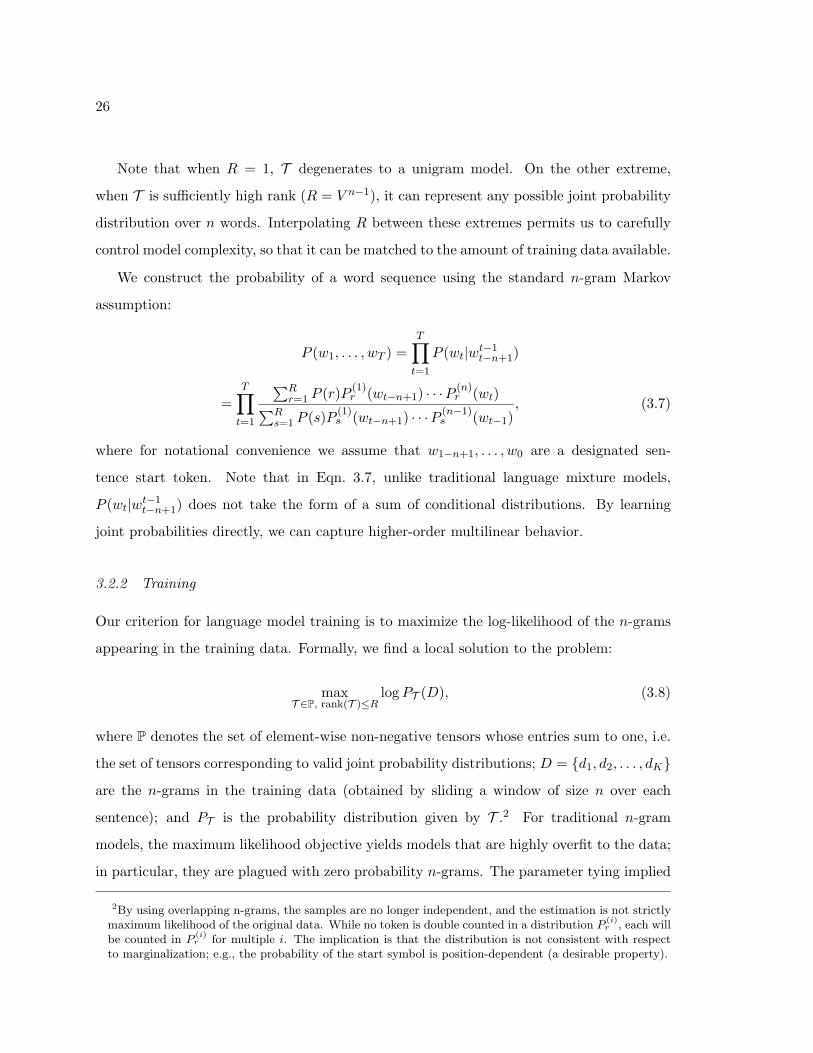
joint probabilities directly, we can capture higher-order multilinear behavior.
3.2.2 Training
Our criterion for language model training is to maximize the log-likelihood of the n-grams
appearing in the training data. Formally, we find a local solution to the problem:
maxT ∈P, rank(T )≤R
logPT (D), (3.8)
where P denotes the set of element-wise non-negative tensors whose entries sum to one, i.e.
the set of tensors corresponding to valid joint probability distributions; D = d1, d2, . . . , dKare the n-grams in the training data (obtained by sliding a window of size n over each
sentence); and PT is the probability distribution given by T .2 For traditional n-gram
models, the maximum likelihood objective yields models that are highly overfit to the data;
in particular, they are plagued with zero probability n-grams. The parameter tying implied
2By using overlapping n-grams, the samples are no longer independent, and the estimation is not strictlymaximum likelihood of the original data. While no token is double counted in a distribution P
(i)r , each will
be counted in P(i)r for multiple i. The implication is that the distribution is not consistent with respect
to marginalization; e.g., the probability of the start symbol is position-dependent (a desirable property).

27
by the low rank form greatly reduces the risk of introducing zero probabilities into the
model; in practice, some additional smoothing is still required.
The low-rank language model can be interpreted as a mixture model, where each compo-
nent is a joint distribution that decomposes into a product of position-dependent unigram
models over words: Pr(wt−n+1, . . . , wt) = P(1)r (wt−n+1) · · ·P (n)
r (wt). Using this interpre-
tation, we propose an expectation-maximization (EM) approach to training our models,
iterating:
1. Given model parameters, assign the responsibilities γrk of each component r to the
k-th n-gram instance dk = (w(k)1 , w
(k)2 , . . . , w
(k)n ):
γrk =P (dk|r)P (r)
P (dk)=P (r)P
(1)r (w
(k)1 ) · · ·P (n)
r (w(k)n )
P (w(k)1 , w
(k)2 , . . . , w
(k)n )
(3.9)
2. Given responsibilities γ, re-estimate F (i), λ:
P (p)r (w) =
∑Kk=1 γrkδ(w
(k)p = w)
∑Kk=1 γrk
(3.10)
P (r) =1
K
K∑
k=1
γrk (3.11)
where δ is an indicator function. Iterations continue until perplexity on a held-out develop-
ment set begins to increase.
The above training is only guaranteed to converge to a local optimum, which means
that proper initialization can be important. A simple initialization is reasonably effective
for bigrams: randomly assign each training sample to one of the R mixture components
and estimate the component statistics similar to step 2. To avoid zeroes in the component
models, a small count mass weighted by the global unigram probability is added to each
distribution P(p)r (w) in Eqn. 3.10.
3.3 English Genre Modeling Experiments
Our expectation is that the LRLM will be good for applications with small training sets.
The experiments here first evaluate the LRLM by training on a small set of conversational

28
Dataset Size (words)
BN Train 3.2M
BC Train 99K
BC Dev 189K
BC Test 136K
Table 3.1: Language model experiment data.
speech transcripts and then in a domain adaptation context, which is another common
approach when there is data sparsity in the target domain. The adaptation strategy is
the standard approach of static mixture modeling, specifically linearly interpolating a large
general model trained on out-of-domain data with the small domain-specific model.
3.3.1 Experimental Setup
Our experiments use LDC English broadcast speech data,3 with broadcast conversations
(BC) or talkshows as the target domain. This in-domain data is divided into three sets:
training, development and test. For the out-of-domain data we use a much larger set of
broadcast news speech, which is more formal in style and less conversational. Table 3.1
summarizes the data sets.
We train several bigram low rank language models (LR2) on the in-domain (BC) data,
tuning the rank (in the range of 25 to 300). Because the initialization is randomized, we
train models for each rank 10 times with different initializations and pick the one that
gives the best performance on the development set. As baselines, we also train in-domain
bigram (B2) and trigram (B3) standard language models with modified Kneser-Ney (mKN)
smoothing. Our general trigram (G3), trained on BN, also uses mKN smoothing. Finally,
each of the in-domain models is interpolated with the general model. We use the SRILM
toolkit [118] to train the mKN models and to perform model interpolation. The vocabulary
consists of the top 5K words in the in-domain (BC) training set.
3http://www.ldc.upenn.edu

29
50 100 150 200 250 300160
165
170
175
180
Rank
Per
plex
ity
Figure 3.2: Low rank language model perplexity by rank.
3.3.2 Results
The experimental results are presented in Table 3.2. As expected, models using only the
small in-domain training data have relatively high perplexities. Of the in-domain-only
models, however, the LRLM gives the best perplexity, 3.6% lower than the best baseline.
Notably, the LR bigram outperforms the mKN trigram. The LR trigram gave no further
gain; extensions to address this are described later. The LRLM results are similar to mKN
when training on the larger BN set.
Benefiting from a larger training set, the out-of-domain model alone is much better than
the small in-domain models. Interpolating the general model with any of the in-domain
models yields an approximately 15% reduction in perplexity over the general model alone,
highlighting the importance of in-domain data. However, the different target-domain models
are contributing complementary information: when the in-domain models are combined
performance further improves. In particular, combining the baseline trigram and LRLM
gives the largest relative reduction in perplexity.
Figure 3.2 reports LRLM perplexity for the LR2 model by rank R (the number of
mixture components). For an in-domain bigram model, using approximately R = 250
mixture components is optimal, which corresponds to roughly 10% as many parameters as
a full bigram joint probability matrix.

30
Model Perplexity
B2 166.7
B3 169.1
LR2 162.9
B2+LR2 154.5
G3 98.7
G3+B2 83.7
G3+B3 83.6
G3+LR2 83.6
G3+B2+LR2 83.1
G3+B3+LR2 82.6
Table 3.2: In-domain test set perplexities. B denotes in-domain baseline model, G denotesgeneral model, and LR denotes in-domain low rank model. Each model is suffixed by itsn-gram order.
3.3.3 Discussion
Each component in the model specializes in some particular language behavior; in this light,
the LRLM is a type of mixture of experts. To gain insight into what the different LRLM
components capture, we investigated likely n-grams for different mixture components. We
find that components tend to specialize in one of four ways: 1) modeling the distribution of
words following a common word, 2) modeling the distribution of words preceding a common
word, 3) modeling sets of n-grams where the words in both positions are relatively inter-
changeable with the other words in the same position, and 4) modeling semantic related
n-grams. Table 3.3 illustrates these four types, showing sample n-grams randomly drawn
from different components of a trained low rank model.

31
r = 53 r = 33 r = 236 r = 122
λr = 1.29e-02 λr = 1.41e-02 λr = 1.26e-02 λr = 1.26e-03
he was down and should be we civilians
he goes over and can be defense security
he says people and will make syrian armed
he faces one and would affect iraqi prison
Table 3.3: Samples drawn randomly from LRLM mixture components.
3.4 Conclusions
Language model smoothing techniques can be viewed as operations on joint probability
tensors over words; in this space, it is observed that one common thread between many
smoothing methods is to reduce, either exactly or approximately, the tensor rank. This
chapter introduces a new approach to language modeling that more directly optimizes the
low rank objective, using a factored low-rank tensor representation of the joint probability
distribution. Using a novel approach to parameter-tying, the LRLM is better suited to
modeling domains where training resources are scarce. On a genre-adaptation task, the
LRLM obtains lower perplexity than the baseline (modified Kneser-Ney-smoothed) models.
Our initial experiments did not obtain gains for trigrams as for bigrams. Possible im-
provements that may address this include alternative initialization methods to find better
local optima (since training optimizes a non-convex objective), exploration of smoothing in
combination with regularization, and other low-rank parameterizations of the model (e.g.
the Tucker decomposition [69]). For domain adaptation, there are many other approaches
that could be leveraged [8], and the LRLM might be useful as the filtering LM used in
selecting data from out-of-domain sources [18]. Finally, it would be possible to incorporate
additional criteria into the LRLM training objective, e.g. minimizing distance to a reference
distribution.

32
Chapter 4
THE SPARSE PLUS LOW-RANK LANGUAGE MODEL
In Chapter 3 we introduced a tensor-based “low rank language model” (LRLM) that
outperforms baseline models when training data is limited. A disadvantage of the LRLM is
that the non-convex objective complicates training. In this chapter, we propose a new model
based on a reparameterization of the maximum entropy modeling (exponential) framework,
side-stepping the limitations of the LRLM and leveraging advantages of exponential models.1
Like existing exponential models, our model can make use of features of words and histories
and training is convex. Unlike existing models, however, we parameterize the model with the
sum of two weight matrices: a low rank matrix that effectively models frequent, productive
sequential patterns, and a sparse matrix that captures exceptional sequences. We will show
that the low rank weight matrix can be interpreted as incorporating a continuous-space
language model into the exponential setting, and will discuss how the sparsity pattern in
the sparse weight matrix can benefit other, important language processing tasks.
We evaluate the model and its properties in a sequence of experiments. First we evaluate
its language modeling performance on English telephone conversations, which allows us to
gain insight into the model’s behavior. We then evaluate the how well the model does
with low resource languages, reporting results using limited training data from Cantonese,
Pashto, Turkish, Tagalog and Vietnamese. To explore the model’s ability to incorporate
non-trivial features of words and histories, we investigate morphological features in further
Turkish language modeling experiments. Finally, we conclude with an analysis of how we
can use learned sparse weights to automatically discover words and multiwords in Cantonese
and Vietnamese.
1Portions of this chapter appeared previously in [56].

33
4.1 Sparse and Low-Rank Language Models
4.1.1 The Model
As described in Chapter 2, the standard exponential language model [101] has the form
p(w|h) = exp(
aT f(w, h))
∑
w′ exp (aT f(w′, h)), (4.1)
where a ∈ Rd are the parameters and f(w, h) ∈ R
d is the feature vector extracted from word
w and history h. We generalize the model with two key changes: i) the vector is recast
as a feature matrix with a corresponding weight matrix A, and ii) the weight matrix A is
decomposed into the sum of two matrices, A = S+L, each of which have special structure.
The basic weight matrix parameterized exponential model can be written as:
p(w|h) = exp(
ψ(w)TAφ(h))
∑
w′ exp (ψ(w′)TAφ(h)). (4.2)
Here ψ(w) ∈ Rdψ is the vector of features of w individually and φ(h) ∈ R
dφ are the features
of h. In this case A ∈ Rdψ×dφ is a parameter matrix. This can be linked to the notation
of Eqn. 4.1 by noting that ψ(w)TAφ(h) = 〈A,ψ(w)φ(h)T 〉, where 〈·, ·〉 denotes a matrix
inner-product (element-wise multiply and sum). If one denotes the vectorization of A with
a and the vectorization of feature matrix ψ(w)φ(h)T with f(w, h), then we can convert
any model of the form Eqn. 4.2 into one of the form of Eqn. 4.1. On the other hand, any
exponential language model of the form Eqn. 4.1 whose features are products of features on
words and histories can transformed into one in the form of Eqn. 4.2. In particular, standard
n-gram features take this form, where ψ(w) and φ(h) are one-hot (indicator) encodings of
the words and histories. In most of our experiments we focus on these standard n-gram
features, though we branch out to morphological features in Sec. 4.5.
Empirically we observe that the weight matrices A learned for models of the form Eqn.
4.2 contain two qualitatively different kinds of information. First, there are relatively dense
regions of the matrix that model the sequential behavior of high frequency words. Because
only a small fraction of the words are frequent, this information can be well modeled by a low
rank matrix. Second, there are large sparse regions of the matrix, where only a handful of
the elements deviate significantly from zero - these correspond to n-grams whose individual

34
20 40 60 80 100 120 140 160 180 200
50
100
150
200
20 40 60 80 100 120 140 160 180 200
50
100
150
200
Figure 4.1: The weight matrix A can be naturally decomposed into sparse (top) and lowrank (bottom) matrices.
words infrequently appear outside of a small handful of n-grams (e.g. “san francisco”).
This information alone can be well modeled by a sparse matrix. Fig. 4.1 illustrates this
result, visualizing the estimated weights in the 200 × 200 leading submatrix of a bigram
weight matrix trained on 100K tokens with a 5K vocabulary. The complete matrix can be
decomposed accurately into the sum of a sparse matrix (S, upper) and low rank matrix (L,
lower). We show in this chapter that language modeling performance can be improved by
using a more general model able to efficiently capture both types of structure inherent in
the data.
Sparse Component
The model of Eqn. 4.1 is often trained with ℓ1 regularization applied to a. Not only is it
well-known that this particular penalty leads to sparse solutions, but it empirically has also
been found to be a good criterion to minimize (in terms of test set perplexity) [28]. An
entry-wise ℓ1 penalty can be applied to a weight matrix S to the same effect. In standard

35
models, the “sparse” component is the only component, and is thus tasked with modeling
all of the sequential behavior; we will see below how our model uses sparsity in a different
way.
Low-Rank Component
Restricting ourselves to a sparse solution ignores an important attribute of language: that
similarities exist between words and between histories in the data. A sparse model has no
way to exploit similarities that might exist (e.g. between the words “bicycle” and “bike”).
Viewed in the form of Eqn. 4.1, this is inevitable: features are values at arbitrary positions
in a vector. Viewed in the form of Eqn. 4.2, we see similarities between two words can be
expressed by similarity between the corresponding rows, and similarities between histories
can be viewed as similarities between the corresponding columns. More generally, sets of
rows (or columns) may live in subspaces, e.g. one might envision a “space” of adjectives,
or a “space” of nouns. This property corresponds to a low rank solution; i.e. finding a low
rank weight matrix A.
Empirically, a low rank component typically appears in the solution without any encour-
agement from the model or training. By facilitating the existence of a low-rank component,
we can improve the modeling performance. For example, the co-occurrence statistics for
a word α that has been observed 50 times may be sufficiently similar to a set of words β
that have been observed hundreds or thousands of times for α’s weights to be pushed into
β’s subspace of weights; in effect, this “fills in” missing entries from α’s weight rows and
columns.2
The idea of learning and exploiting similarities between objects (e.g. words and histories)
is a common theme in the literature on learning shared representations [3] and is used
by language models with continuous representations of words, particularly neural network
language models [10, 106]. We show here that an exponential model with a low rank weight
matrix A is in fact a continuous-space language model. To see this, note that A ∈ Rdψ×dφ
with rank R ≤ min(dψ, dφ) has a singular value decomposition A = UΣV T , with diagonal
2This basic idea is extensively exploited in low-rank matrix completion approaches to collaborative filter-ing, as discussed in Chapter 2.

36
matrix of singular values Σ ∈ RR×R, left singular vectors U ∈ R
dψ×R and right singular
vectors V ∈ Rdφ×R. Substituting the structure of A into Eqn. 4.2, we get
p(w|h) =1
Z(h)exp
(
ψ(w)TUΣV Tφ(h))
(4.3)
=1
Z(h)exp
((
UTψ(w))
Σ(
V Tφ(h)))
(4.4)
=1
Z(h)exp
(
ψ(w)TΣφ(h))
. (4.5)
Here ψ(w) = UTψ(w) denotes a continuous, low-dimensional representation of w, φ(w) =
V Tφ(h) denotes a continuous, low-dimensional representation of h, and Z(h) is the normal-
izing factor. The probability of a word following a history is proportional to the weighted
inner-product ψ(w)TΣφ(h) in the low-dimensional space. A illustrative example is given in
Fig. 4.2, which plots the hypothetical continuous representation of three different histories
and three different prediction position words; the inner products induced by this embed-
ding means that “next Tuesday” and “next Thursday” (with a positive inner product) are
probable sequences, while “orange Tuesday” and “orange Thursday” (with a negative inner
product) are not. The dimension of the continuous representation is equal to R, the rank;
lower rank solutions for A correspond to embeddings of words in lower dimensional spaces.
Similar words will have continuous representations that are close to each other in the low-
dimensional space; the same is true for similar histories. Crucially, the low dimensional
representation of a word can (and should) be different in the history position h than in the
predictive position w. In Section 4.1.2, we present an algorithm that discriminatively learns
a low rank matrix, and thus discriminatively learns low dimensional continuous representa-
tions of words and histories.
When A is low rank, the model of Eqn. 4.2 bears some similarity to Mnih and Hinton’s
“log-bilinear” language model [90], which estimates a matrix that is analogous to our U in
Eqn. 4.4, and matrices analogous to V for each word in a fixed history window. In doing
so, they find continuous low-dimensional representations of words and history words. A
few advantages of our approach are that 1) we are guaranteed to converge to a globally
optimal solution, 2) we support arbitrary feature functions of words and histories, and 3)
the dimension of the hidden representation is learned, rather than pre-specified.

37
Figure 4.2: Illustration of continuous, low-dimensional representations of words (blue) andhistories (red). The weighted inner products between these representations determines theprobability of the word following the history. Note that similar words (e.g. days of theweek) naturally cluster together; the same is true of histories.
Sparse and Low-Rank Combination
It is not plausible that all regularities in the data can be learned from a finite training set.
For example, if a word is observed only a handful of times, we may simply not know enough
about it to know what subspace of words it lives in. Further, some n-grams (e.g. proper
nouns, idioms, etc.) do not fit into any regular pattern. A low rank matrix is not well suited
to capture all of these exceptions. Thus we propose a hybrid model, where the weight matrix
A is the sum of two individual components: a low rank matrix L and a sparse matrix S.
The low rank component is free to model all of the regularities present in the data (a result
of the inherent structure present in language). The sparse component learns the rest - the
exceptions to the rule. Unlike the traditional use of sparse weights in an exponential model,
our sparse matrix does not need to allocate any weights to regular, productive patterns
(e.g. it does not need to model n-grams easily explained by part-of-speech constraints).
Our proposed sparse plus low rank language model (SLR-LM) thus has the following form:
p(w|h) = exp(
ψ(w)T (S + L)φ(h))
∑
w′ exp (ψ(w′)T (S + L)φ(h)). (4.6)
As a byproduct of learning, the SLR-LM separates n-grams into two qualitatively dif-
ferent sets: the regular low rank n-grams which are well predicted by the regular rules, and
the sparse n-grams that are not. There are auxiliary benefits to this decomposition. For

38
example, Min et al. [89] show that applying a sparse plus low rank decomposition directly
to a word-document matrix can be used to extract document keywords; in Chapter 5 we
consider similar applications of the n-grams in our sparse matrix.
4.1.2 Training Algorithm
To train the SLR-LM of Eqn. 4.6 we solve the following non-smooth convex optimization
problem:
minS,L
γ0‖L‖∗ + γ1‖S‖1 + γ2‖S + L‖2F − L(X ;S,L). (4.7)
The entry-wise ℓ1 norm, ‖S‖1, promotes sparsity in our S variables. We penalize L’s nuclear
norm, ‖L‖∗, which is known to encourage low rank solutions [47, 99]. The Frobenius norm
permits standard ℓ2-norm regularization. L denotes the average log-likelihood, which has
the familiar empirical-minus-model expectation form for its gradient as a function of A:
∇AL = Ep(w,h)[ψ(w)φ(h)T ]− EpA(w,h)[ψ(w)φ(h)T ]. (4.8)
In Alg. 2 we introduce an iterative algorithm for solving the above convex optimization
problem. The basic structure of each iteration is to make four updates: 1) a gradient step
on S, 2) an entry-wise threshold step to shrink the entries of S, 3) a gradient step on
L, and 4) a singular-value threshold step on L. Both thresholding steps make use of the
soft-thresholding operator:
Sµ(X) = sgn(X) max(0, |X| − µ) (4.9)
where all operations are entry-wise; in particular, denotes entry-wise multiplication. Our
algorithm is a block-coordinate variant of the accelerated proximal gradient descent algo-
rithm introduced by Toh and Yun in [123] (see Alg. 1 in Chapter 2), modified to alternate
between the ℓ1 and ‖ · ‖∗ regularized terms.
4.1.3 Computational Complexity
Compared to standard exponential language model training, the SVD increases the com-
putational cost, adding a O(dψdφRk) term to the per-iteration complexity, where Rk is the

39
Algorithm 2: TrainSLR-LM()
1: S ← L← S′ ← L′ = 0; t← t′ ← 1
2: while not converged do
3: mL← L′ + ((t′ − 1)/t)(L− L′)
4: mS ← S′ + ((t′ − 1)/t)(S − S′)
5: mA← mL+mS
6: Pick τS
7: gS ← mS + (1/τS)∇mA(L − γ2‖mA‖2F )8: pS ← Sγ1/τS (gS)9: S′ ← S and S ← pS
10: sA← mL+ pS
11: Pick τL
12: gL← mL+ (1/τL)∇sA(L − γ2‖sA‖2F )13: [U,Σ, V ]← SVD(gL)
14: pL = USγ0/τL(Σ)V T
15: L′ ← L and L← pL
16: t′ ← t and t← (1 +√1 + 4t2)/2
17: end while
rank of L at iteration k. To speed up training, we employ many of the tricks proposed in
[123], including computing partial SVDs (with PROPACK [71]) and using a continuation
technique that gradually decreases the γ0 and γ1 weights from a large initial value to their
intended target values. The τS and τL parameters in Alg. 2 are picked according to a line
search analogous to Toh and Yun’s. All training computation can be phrased as matrix
operations, permitting us to locally parallelize computation over many cores.

40
4.2 English Language Modeling Experiments
4.2.1 Experimental details
All of our English experiments use telephone conversations from the Fisher corpus [41].
Each conversation in the corpus is labeled by topic; we draw data from eight of the topics
(see Table 4.1) that had at least 350K word tokens. For each topic, we split the data (at the
granularity of conversation) into training, development and test sets, at a 60/20/20 ratio.
To avoid conflating the effects of topic and training set size, after basic text normalization we
subsampled the training data (by sentence) to create three training subsets per topic, with
roughly 200K, 100K and 25K word tokens, respectively. Due to limited training data, we
restrict our vocabulary to the most frequency 5K word types; all out-of-vocabulary tokens
are mapped to a dedicated OOV symbol.
For each topic and training set size, we train a bigram language model on the training set,
use the development data to tune the regularization weights γ0 and γ1 (we fixed γ2 = 0), and
evaluate on the test set. Our first baseline is a “standard” ℓ1 regularized bigram exponential
(Exp) language model, trained as an SLR-LM with γ0 chosen such that the low rank matrix
is zero. Our second baseline is a modified Kneser-Ney (mKN) smoothed bigram language
model.
4.2.2 Results and Discussion
The results are presented in Table 4.2. As expected, in all cases the optimal SLR-LM has
a lower perplexity than the baseline ℓ1 regularized model. Fig. 4.3, which plots the percent
perplexity reduction over the Exp baseline by topic and training set size, makes it easier
to see the overall trends. In particular, although gains are observed at all configurations,
the biggest gains are achieved on the 100K data set size. Presumably, when there is very
little training data (25K), it is difficult to learn the patterns in the data simply because too
few instances are observed. In other words, we observe a rough skeleton of the true matrix,
with too many holes to be accurately filled by the low rank component. On the other hand,
as the amount of training data grows, there become enough examples that the patterns can
be captured by the aggregation of “exceptions”; that is, the patterns in the matrix become

41
Topic # Test Tokens Test OOV Description
ENG01 158K 3.5% Professional sports
ENG02 157K 4.4% Pets
ENG03 130K 2.9% Life partners
ENG04 151K 3.2% Minimum wage
ENG05 131K 3.9% Comedy
ENG24 63K 3.6% September 11
ENG30 76K 3.8% Family
ENG37 81K 3.3% Reality TV
Table 4.1: Topics used from the Fisher corpus.
25K 100K 200K
Topic SLR Exp mKN SLR Exp mKN SLR Exp mKN
ENG01 109.4 109.9 114.6 83.0 86.5 91.6 76.7 78.8 83.4
ENG02 115.1 116.6 126.8 86.6 91.9 97.2 79.5 83.1 87.9
ENG03 116.7 119.6 125.0 88.0 92.6 96.9 80.9 83.7 88.2
ENG04 109.2 110.4 114.3 82.3 85.2 90.8 75.4 77.3 81.8
ENG05 110.2 111.3 118.5 83.4 86.4 91.9 75.4 78.4 82.9
ENG24 125.7 126.8 129.4 93.6 98.0 102.8 85.7 88.6 93.3
ENG30 114.9 116.8 123.4 86.5 90.6 96.3 79.5 83.4 86.8
ENG37 112.5 114.0 116.0 84.1 88.1 92.5 77.8 80.9 84.8
Table 4.2: Test set perplexity by topic and training set size.

42
Figure 4.3: Percent perplexity reduction over Exp baseline by topic and training set size.
dense enough that there are few holes left for the low rank component to fill. Again, the
SLR-LM still outperforms the standard Exp-LM in these cases, just by a smaller margin.
We looked at the high and low weight entries (n-grams) learned for the sparse and low
rank components for a model trained on the topic “minimum wage.” The sparse component,
which models the exceptions in the data, typically learned common noun phrases, including
locations (“new york”, “united states”) and topic-related phrases (“social security”, “gro-
cery store”). Note that nothing prevents the sparse component from having large negative
weight entries to revise the probabilities of n-grams downward, although empirically this
behavior is less common than positive revisions. The low rank component assigned high
weights to n-grams that are syntactically plausible and semantically coherent (“you know,”
“I think,” “I don’t”), and low weights to ones that are not (“the a,” “my that”).
If the SLR-LM is indeed learning a low-dimensional continuous representation, words (or
histories) that function similarly should be mapped close to each other in the continuous
representation. Using a model trained with 200K tokens on the topic of “pets,” we list
in Table 4.3 several words and histories with their nearest neighbors in the low dimension
space. Note that sometimes a word’s neighbors are similar in either position (e.g. “would”),
but they need not be (e.g. “but”). As expected, natural clusters form, e.g. numbers.

43
History Word h Nearest Neighbors
would could, didn’t, can’t, don’t, should
but well, mean, because, guess, think
of from, for, at, in, make
Prediction Word x Nearest Neighbors
would can, did, don’t, didn’t, should, could
but so, because, now, for, as
know keep, think, want, get, talk
one two, four, three, ten, five
dog cat, thing, ones, animal, baby
Table 4.3: Words, histories, and their nearest neighbors in the continuous-space embeddingsinduced by the low rank component from the 200K ENG02 set.
Although our approach to finding low dimensional representations bears a superficial
similarity to Latent Semantic Analysis (LSA) [42], they are learned in very different ways
and optimize different objectives. LSA compiles a word-document co-occurrence matrix and
takes a single truncated singular value decomposition, which minimizes the Frobenius norm
between the original and low rank matrices, to induce semantic similarity between words
based on their co-occurrence within documents. In contrast, training our model iteratively
learns low dimensional representations of words and histories jointly in order to maximize
the log-likelihood of a parametric distribution whose probabilities are governed by weighted
inner products between the low dimensional representations. In our model, the singular
value decomposition is computed on the low rank weight matrix, and not on any empirical
counts from the data directly.
4.3 Low Resource Language Modeling Experiments
As the English language modeling experiment results in Table 4.2 indicate, the SLR-LM
can aid performance when training data is limited (which is when exploiting the similarities
between words and histories is most beneficial). For English, many common scenarios

44
do not involve limited training data; in fact, a fair amount of English language modeling
research involves scaling models to massive datasets. However, limited training data is the
norm for many so called “low resource languages,” which lack the corpora and tools that
are available for languages like English, Mandarin and Modern Standard Arabic. In this
section we conduct language modeling experiments in low resource conditions.
We employ corpora from a diverse set of five languages (Cantonese, Pashto, Turkish,
Tagalog and Vietnamese) to evaluate the SLR-LM’s performance in the limited data condi-
tion. Our corpora consist of transcribed telephone conversations and are distributed through
the IARPA Babel program3 Specifically, we use the “Limited Language Pack” version of
the data for each language, where only roughly 10 hours of speech is available for training.
After text normalization to lower-case the data and remove word fragments, unintelligible
speech and most non-speech tokens, our data sets statistics are summarized in Table 4.4.
Note the large variation in vocabulary size and OOV rate.
For each language we train a bigram SLR-LM. Unlike previous experiments, OOV words
are not mapped to an OOV token: our models never predict OOVs and they break history
context (OOVs at test time are not included in the perplexity computation). At a very
coarse level we tune the regularization weights (γ0, γ1 and γ2) on a small development set,
and evaluate on the test set. As a baseline, we also train modified Kneser-Ney bigram
models on the language models, treating OOVs in the same fashion.
The perplexity results of our model are listed in Table 4.5. On all languages the SLR-LM
beats the baseline model, with an average of a 7.1% reduction in perplexity. This reduction
is consistent with the reduction observed in English, and supports the idea that the SLR-LM
is an appropriate model to use when training data is limited.
4.4 Comparison with other Continuous Space Models
As discussed in Chapter 2, there are other continuous-space language models. Though we
do not have direct comparisons to these models on our data, we present in this section some
3We use the Cantonese language collection release babel101b-v0.4c sub-train1, the Pashto language col-lection release babel104b-v0.4bY, the Turkish language collection babel105b-v0.4, the Tagalog languagecollection release babel106b-v0.2g-sub-train, and the Vietnamese language collection release babel107b-v0.7.

45
Language # Training Tokens # Test Tokens Vocab Size OOV Rate
Cantonese 98.9k 17.0k 5.0k 7.4%
Pashto 111.0k 36.4k 6.2k 5.2%
Turkish 70.8k 24.1k 10.1k 15.4%
Tagalog 68.3k 23.4k 5.5k 9.1%
Vietnamese 115.5k 41.2k 2.9k 1.4%
Table 4.4: Statistics of the low resource language data used in our language modeling work,which come from the “Limited Language Pack” portions of the data collection releases forthe IARPA Babel program.
Language mKN Perplexity SLR-LM Perplexity
Cantonese 112.7 103.3
Pashto 159.0 145.9
Turkish 246.5 234.6
Tagalog 123.3 113.0
Vietnamese 176.7 166.2
Table 4.5: Language modeling performance across languages, comparing a modified Kneser-Ney (mKN) baseline to the SLR-LM.

46
Ppl Reduction
Model n Alone Interpolated
Neural Net (NN) 5 0.7% 17.4%
Log-Bilinear 5 -2.3% 18.4%
Recurrent NN - 11.7% 25.1%
RNN-LDA - 19.5% 30.4%
Table 4.6: Perplexity reductions reported in [85] with the Penn Treebank corpus (930Ktraining tokens).
Ppl Reduction
Model n Alone Interpolated
NN 4 9.2% -
Deep NN 4 10.1% 19.3%
Table 4.7: Perplexity reductions reported in [6] with the Penn Treebank corpus (930Ktraining tokens).
recent results from the literature to give context for the kinds of gain researchers achieve
over baselines.
In Table 4.6, we summarize results included in [85]. The “Alone” column lists the relative
reduction in perplexity over a baseline modified-Kneser-Ney 5-gram using the listed model
only, while the interpolated column shows the improvement when the individual model is
also interpolated with the baseline. Alone, the neural network language model gives very
little gain, and the log-bilinear model [90] actually hurts performance. It is only with in-
terpolation do they get large gains. In contrast, the reductions we reported in previous
sections, between 5.6% to 9.5%, are obtained using our model alone with no interpolation.
Zweig and Mikolov report two recurrent neural network (RNN) results: the first a “stan-
dard” RNN and the latter one that also uses topic information as learned by latent Dirichlet

47
allocation [14] as an input feature. Both give strong improvements, particularly with inter-
polation. These large improvements are typical of recurrent neural network models, though
as mentioned in Chapter 2, the arbitrary history length precludes their practical use in
speech recognition decoding and lattice rescoring. Table 4.7 reports a few additional data
points from [6] on a larger training set, showing improvements around 10% alone. Again,
the improvements reported in Tables 4.6 and 4.7 are not directly comparable to ours, since
they use different datasets (with different sizes, languages and genres), but do give a sense
of the kinds of improvements being obtained by state-of-the-art continuous space models.
In Table 4.8, we summarize the relative advantages and disadvantages of the SLR-LM
relative to other classes of language model. The “Pros” refer to places where the SLR-LM
is stronger, and “Cons” where it is at a disadvantage. That the SLR-LM learns sparse
exceptions, which will be shown to be meaningful for other language processing tasks, is an
advantage over all of the comparison language models listed. Relative to n-gram language
models in particular, the SLR-LM is better able to smooth, in part due to its continuous
space nature and in part to its ability to incorporate features. This comes at the cost of
training complexity and ease of integrating into speech recognition decoding, both of which
favor the n-gram model. Compared to maximum entropy and Model M language models,
the SLR-LM has the advantage of being a continuous space model, but is slower to train
and requires more memory. In favor of the SLR-LM relative to neural network language
models (include deep and recurrent ones) is its ability to use features of the prediction
word, its convex training objective and that it learns the dimensionality of the continuous
representation automatically. Unlike the deep or recurrent neural networks, the SLR-LM is
unable to learn deep representations of histories. Unlike recurrent neural networks, the SLR-
LM can only exploit arbitrarily long histories through features. Finally, compared to the
log-bilinear model, the SLR-LM is convex and learns the dimensionality of the continuous
representation, but since it does not factor the weights, it is less scalable. There are some
attributes that could be interpreted as either an advantage or disadvantage. For example,
the SLR-LM has a simpler form compared to neural network language models, which makes
training easier but limits the capacity of the continuous space mapping. Likewise, the fact
that recurrent neural network language models have arbitrarily long histories is an advantage

48
SLR-LM Compared to Standard n-gram LMs
Pros Cons
Able to exploit similarities (better smoothing) Far less scalable
Supports features (word and history) Harder to integrate into decoding
Able to identify exceptional n-grams
SLR-LM Compared to Maximum Entropy and Model M LMs
Pros Cons
Able to exploit similarities (better smoothing) Less scalable
Able to identify exceptional n-grams
SLR-LM Compared to Neural Network LMs
Pros Cons
Convex (easier training) Cannot learn deep representations
Able to incorporate features of prediction word Harder to exploit arbitrarily long history
Dimensionality of continuous representation is learned
Able to identify exceptional n-grams
SLR-LM Compared to the Log-Bilinear LM
Pros Cons
Convex (easier training) Less scalable
Dimensionality of continuous representation is learned
Able to identify exceptional n-grams
Table 4.8: Summary of key differences between the SLR-LM and other language models.Pros refer to advantages of the SLR-LM; cons refer to limitations of the SLR-LM.

49
in terms of modeling power, but limits the scenarios in which they can be used.
4.5 Turkish Morphological Language Modeling Experiments
Highly agglutinating languages are challenging to model due to the substantial vocabulary
sizes. One common strategy for grappling with this challenge is to incorporate morphological
information, allowing information to be pooled over related sets of words (e.g. those with
a shared inflectional affix). One nice property that the SLR-LM shares with the ME-LM is
the ability to incorporate arbitrary features of words and of histories [100]. In this section
we explore the use of morphology as features in a SLR-LM on conversational Turkish data,
which exhibits extensive agglutination. It is important to note that the units of our language
model are words, not morphemes; we use morphological information only as a feature.
There are several ways in which morphology can be used as features. If the morphology
is concatenative, one might decompose a word into its constituent morphemes and treat the
presence of a morpheme as a feature for that word; for example, by representing a word
as an indicator vector of its morphological constituents. In highly agglutinating languages,
it may be reasonable to treat sequences of affixes as a single affix bundle, in which case
there would be features indicating the stem and any affix bundles (prefix or suffix). Non-
concatenative morphological phenomena can be handled as well; for example, in language
with reduplication a single binary reduplication feature can be added to the morphological
feature vector to indicate whether the word does or does not contain reduplication. In
cases of templatic morphology, as in Arabic, one might indicate the stem and the template.
Beyond the issue of the way in which a word can be decomposed into morphological elements,
there is the issue of how and when to include it as a feature. One can use only features of
the history or features of the word, or both. Empirically in pilot studies, we find that using
features of the word can lead to overly smoothed probability distributions. Features of the
history typically decompose into features over individual history words. The features of
the history words can be stacked (so that the overall history vector is the concatenation of
per-history-word feature vectors), which preserves sequencing information, or they can be
merged in a “bag-of-morphs” style, where one only indicates whether a morpheme appeared

50
babandan Original Form
babLndLn After vowel harmony normalization
babL +n +dL +n After morphological decomposition
Figure 4.4: Example Morfessor morphological decomposition of Turkish word “babandan”(father). This decomposition yields one stem feature (“babL”) and two suffix features(“+dL” and “+n”) for the word.
or not anywhere in the history window.4 The effectiveness of the two styles will depend on
the language: the freer the word order the more appropriate the bag-of-morphs modeling
assumption is. The bag-of-morphs style has a computational advantage, since it leads to a
lower history feature dimension.
4.5.1 Experimental details
Data
Our Turkish data comes from the IARPA Babel project (Turkish data collection release
babel105b-v0.4) and consists of telephone conversation transcripts. For language modeling,
we use the provided “Limited Language Pack” (LLP) training set which, after removing
non-speech tokens and lower-casing, has a 10k word vocabulary despite only containing 70k
training tokens. We tune our models using a 23k word development set that is a subset of
the official 70k development set, and evaluate on a different 24k word subset (the subsets
were automatically selected to balance dialect and gender characteristics).
Morphological Decomposition
We use an unsupervised morphological decomposition learned on the “Full Language Pack”
(IARPA Babel Turkish data collection release babel105b-v0.4) which consists of 38k word
types and 554k word tokens.5 It uses the Morfessor tool [36] to learn the decomposition,
4We thank Janet Pierrehumbert for the suggesting features that ignore word order, motivated by Turkish.
5In addition to our appreciation for providing this decomposition, we would also like to thank PeterBaumann and Janet Pierrehumbert for their advice on choices of features and insights in the interpretation

51
after the vocabulary was first pre-processed to normalize orthography for vowel harmony
(another notable feature of Turkish) [7]. Fig. 4.4 illustrates the way in which a word might
be decomposed into morphological constituents. Each distinct morpheme will serve as a
feature, as described next.
Features
In these experiments, our representation of the history, φ(h) =[
φ(w−(n−1))T , . . . , φ(w−1)
T]T
,
is the concatenation of vector representations of each word in the history. The vector rep-
resentation of the kth most recent history word, φ(w−k), is (V +M)-dimensional, where V
is the number of words in the vocabulary and M is the number of distinct sub-word units
(e.g. morphemes) observed in the decomposition of the vocabulary. Then φ(w−k) is a sparse
binary vector with a 1 indicating the word identity and 1s indicating each of its constituent
sub-word units. As our experiments will show, feature pruning is an useful step in order to
obtain good performance. We rely on three criteria for pruning:
1. First, a morphological feature must appear in a sufficient number of word types.
Without any cutoff, it is possible that a morphological feature only appears in a single
word type, in which case it provides no additional information over the word identity
itself.
2. Second, a morphological feature must appear in a sufficient number of word train-
ing tokens. This simply ensures that the weights for the feature can be estimated
effectively.
3. Finally, we also consider excluding certain classes of morphemes; e.g. stems. For
example, with a bigram model, the local sequencing is largely influenced by part of
speech, which is better captured with affix morphemes or affix bundles. In contrast,
stems are poor for local sequencing information, because they can be present with
different parts of speech, reducing their utility as a predictor of an upcoming word.
of the results.

52
Morpheme Units Type Cutoff Token Cutoff Perplexity
None - - 234.7
2g stem, 2g affix None None 237.2
2g stem, 2g affix 5 20 235.3
2g affix None None 232.3
2g affix 5 20 231.6
10g B-o-S, 2g affix None None 231.6
10g B-o-S, 2g affix 5 20 233.1
Table 4.9: Language modeling results with different morphological feature sets. ng denotesn-gram and B-o-S denotes “bag of stems.” A bigram modified-Kneser Ney model on wordsgives a perplexity of 246.5, while a bigram Factored Language Model with affix featuresgives a perplexity of 241.9.
The thresholds for criteria 1 and 2 are loosely tuned on our development set.
4.5.2 Results and Analysis
Using the LLP training data, we estimate train several variants of morphological-feature
SLR-LMs. The results are listed in Table 4.9. First, the baseline SLR-LM that uses no
morphological features achieves a perplexity of 234.7. The second block of the table includes
results with the unsupervised Morfessor decomposition features. Adding bigram stem and
affix features without pruning yields a perplexity of 237.2 (though this is improved to 235.3
when stem and affixes are pruned by type and token frequency). Excluding stem features,
which risk conflating noun, verb and other part-of-speech contexts, improves performance
to 232.3. Finally, with a pruned affix feature set yields a perplexity of 231.6. A 10-gram
bag-of-stem features with bigram affix features neither helps nor hurts performance, despite
needing no pruning. When the features are pruned, performance slightly degrades. These
results outperform our two baselines: a bigram modified-Kneser Ney model on words, which
gives a perplexity of 246.5, and a bigram Factored Language Model with affix features, which
gives a perplexity of 241.9.

53
To gain intuition into how morphological features are being used in the model, we
plotted the low rank and sparse weights for morpheme and word features (i.e. the ℓ2 norms
of the rows of L and S) for the “2g affix” model with token and type cutoffs of 20 and 5,
respectively. As shown in Fig. 4.5, morphological features are more naturally modeled by
the low rank matrix (in comparison to word features). This distinction between morpheme
and word features suggests two possible explanations: 1) the way that morpheme and words
function in the history may be qualitatively too different to effectively map down into the
same low-dimensional space, forcing the low rank and sparse matrices to model different
kinds of features, and 2) the morphological features yield more regular sequential patterns,
and are thus more naturally suited to the low rank matrix.
Ours is not the first model to incorporate morphological features. One of our baseline
models, the Factored Language Model (FLM) [12], was discussed in Chapter 2. It maps each
word to a set of factors; for example, mapping an Arabic word to a stem, root and pattern.
Our approach shares with the FLM the idea that expressing a word as a set of sub-parts can
lead to more reliable estimation for morphologically rich languages. There are a number of
key differences, though: the SLR-LM is an exponential model while the FLM is an n-gram
model, the FLM assumes a fixed number of “factors” while in the SLR-LM a word can
map to a variable number of features (as long as the feature vector dimension is fixed),
and the SLR-LM provides a mechanism for learning similarities and exceptions within the
morphological feature space, which is not supported by the FLM. The Factored Neural
Language Model [2] uses morphology more closely to the way we use it; namely, it treats
morphology as features. The modeling assumptions are fairly different, though, due to the
underlying differences between neural networks and exponential models, and while FNLM
can learn low-dimensional representations of morphological features (in the history, at least),
it has no mechanism for learning exceptions. Others have introduced sophisticated and
effective language models in the exponential framework that use morphological information
[108, 103], but like the FNLM, they do not learn low dimensional representations nor can
they find exceptions.

54
Figure 4.5: For each history feature in a trained morphological SLR-LM, the ℓ2 norm of theweights are plotted (morphological features in red circles; word features in blue x’s).

55
4.6 Word and Multiword Learning Experiments
In the writing systems of most languages, words are delimited with white space, but this
is not universal. Mandarin and Cantonese, for example, are often written without any
whitespace. For consistency, Vietnamese is often written at the syllable level. In both cases,
the easiest unit to work with is the syllable, since this is the only deterministic segmentation
available that does not rely on external linguistic knowledge. This is problematic for speech
recognition for two reasons: first, syllable-based language models tend to be weak, since for
any given n the n-gram context covers less of the full history, and second, shorter units have
fewer distinguishing components and are thus more prone to accidental insertion, deletion or
substitution. It is desirable, therefore, to take a syllable-level representation of language and
automatically convert it into one that includes multi-syllable units, which typically would
be word or multiword units. It is even better for the low-resource case if the technique
for identifying words and multiwords is entirely automatic and makes no use of language
knowledge. This is the problem we tackle in this section.
One very important characteristic of the SLR-LM is that its weight structure reveals
something about language; in particular, the sparse plus low rank structure decomposes
language into exceptional n-grams and productive n-grams. In this section, we see how
the sparse elements in a language model over sub-word units (i.e. syllables) can automat-
ically identify words and multiwords in the language. We compare what it learns against
and combine with several other state-of-the-art techniques, and evaluate both in terms of
language modeling performance and in the rate at which it identifies actual words.
4.6.1 Experimental details
As mentioned above, we will consider two syllable segmented languages: Cantonese and
Vietnamese. Our data come from the IARPA Babel program (Cantonese data collection
release babel101b-v0.4c sub-train1 and Vietnamese data collection release babel107b-v0.7).
We use the “Full Language Pack” training sets with roughly 100 hours of training data per
language. The Vietnamese data comes syllable segmented, while for Cantonese the data
comes word segmented. To simulate more typical conditions, we converted the Cantonese

56
text into a character-segmented form (leaving foreign words with roman character sequences
intact). The data set and vocabulary sizes are summarized in Table 4.10.
Using the training data, we generate several ranked lists of candidate multiwords ac-
cording to the following methods.
• SLR-LM (slrlm). To obtain these, we first train a bigram SLR-LM on the syllable- or
character-level data. After the model has been tuned, we take the positive elements of
the sparse weight matrix to be our candidate (bigram) multiwords. The list is sorted
by the magnitude of the entries, from largest to smallest.
• Bigram product (bp). Drawing from the literature on multiword learning [102], we
compute the bigram product p(w1, w2)/√
(p(w1)p(w2)) for all bigrams w1w2 in the
training data, and sort the list from largest to smallest. (Bigram product was shown
to work better than mutual information in [102].) With some manipulation, this can
be shown to give an equivalent ranking as taking the product of the probability of the
first word given the second and the probability of the second word given the first. In
either form, it clearly favors bigrams whose relative frequency of occurring together is
high.
• Adaptor Grammar (ag).6 Adaptor Grammars [62] are a framework for defining a
variety of non-parametric hierarchical Bayesian models that delivers state-of-the-art
performance on unsupervised word segmentation of phonemically transcribed child di-
rected speech [63]. Here we investigated two different “collocation” adaptor grammars
for resegmenting the training data. Both these models capture inter-word dependen-
cies by learning larger-than-word units (see [65] for details). The resulting segmenta-
tion is used to identify potential multiwords to be added to the lexicon. Following the
methodology outlined in [65], we used minimum Bayes risk decoding and put fixed
priors on all hyper-parameters instead of manually tuning model parameters.
6We thank Mark Johnson and Benjamin Borschinger both for providing our Adaptor Grammar multiwordcandidate lists and for providing this paragraph describing Adaptor Grammars.

57
Language Units Training Tokens Dev Tokens Test Tokens Vocab Size
Vietnamese Syllables 890k 40.7k 38.7k 5.2k
Cantonese Characters 970k 21.1k 78.1k 3.5k
Table 4.10: Description of data for the word and multiword learning experiments. For Can-tonese, the character-level segmentation is obtain by splitting an original word segmentationto simulate unsegmented conditions.
• Frequency (freq). This simple baseline sorts all bigrams in the training data by their
frequency of occurrence.
• Pronunciation variability (pron).7 This method finds adjacent token sequences that
most often exhibit non-standard pronunciations, where non-standard pronunciations
are found by first performing a forced alignment of the training text, and then marking
as non-standard any candidate multiword that contains at least one phoneme with
pronunciation variation (defined to be phones whose average per-frame acoustic score
is at least two standard deviations under the model mean for that triphone).
• Voting. We consider a simple voting strategy, where several multiword lists are taken
as input. Each list is truncated to the top K candidate multiwords, and then each of
the lists “vote” for their K multiwords. The combination sorts multiwords by vote
count, so any candidate multiword that appeared in all lists would appear before any
candidate multiword that appeared in all but one list, and so forth. Multiwords with
the same vote count are sorted by their bigram product score.
• Zipper. An even simpler combination method is also considered. This combination
approach walks round-robin through the input lists, first taking the top entries in
each, then the second entries in each, and so forth (candidate multiwords are only
added the first time they are encountered).
7We thank Rohit Prabhavalkar, Yanzhang He and Eric Fosler-Lussier at Ohio State University for con-ducting the pronunciation variability analyses and for providing the corresponding lists.

58
4.6.2 Results and Discussion
We first evaluate how well each method does at identifying words in the language. Specif-
ically, for each list, we take the top N entries and see which percentage of the candidate
multiwords (recall that these are actually multisyllables or multicharacters) appear in an
external dictionary,8 and vary N . Note that precision with an external dictionary is an
imperfect criterion, since there is no guarantee that the dictionaries have perfect cover-
age, especially of valid multiwords. In a limited analysis, we took the top 25 hypothesized
words for the ag, slrlm and bp methods that were not in the dictionary and asked native
speakers of Cantonese and Vietnamese to evaluate them.9 The native Vietnamese speaker
indicated that 84% of the hypothesized words were actually valid words or multiwords. In
Cantonese, 58% were deemed valid words (often nouns shared with Mandarin), 15% deemed
valid multiwords (typically Cantonese spoken expressions) and 27% neither valid words nor
multiwords. Because of the noisy nature of this statistic, we consider only large differences
meaningful.
The results are shown in Figs. 4.6 and 4.7. Our analysis of the dictionary does not suggest
that fixing the dictionary would bias in favor of one method or the other, but does suggest
that the performance is stronger in general than these figures indicate. For Cantonese,
the voting combination of bp, slrlm and ag is the clear winner for all list sizes. Selecting
multiwords by pronunciation variability performs poorly; it may be that the variation is
often attributable to dialect instead of within-word reduction. The frequency criterion,
as expected, is quite poor at identifying words. The overall trends are quite similar for
Vietnamese, with the exception that voting does not help and the ag method is somewhat
weaker.
Next, we evaluate how word and multiword learning can be used to improve language
modeling. By selectively joining syllables or characters into words, both the vocabulary
size and the average effective history context increases. The process is simple: 1) given a
multiword list we resegment the training and test data, joining pairs of syllables or characters
8Cantonese dictionary: http://kaifangcidian.com/xiazai/ (33.3k words).Vietnamese dictionary: http://vlsp.vietlp.org/ (31.1k words).
9We thank Yanzhang He and Van Hai Do for performing these analyses.

59
0
0.2
0.4
0.6
0.8
1
0 500 1000 1500 2000
Fra
ctio
n of
Mul
tiwor
ds in
Dic
tiona
ry
Cumulative # Multiwords Added
Cantonese Dictionary Hit Rates
Voting (bp+slrlm+ag)Zipper (bp+slrlm)
Bigram ProductSLR-LM
Adaptor GrammarFrequency
Pronunciation Var
Figure 4.6: The proportion of Cantonese “multiwords” (words) found in an external dictio-nary as the number of multiwords grows, for different multiword lists. Methods comparedinclude SLR-LM, Bigram Product, Adaptor Grammar, Frequency, Pronunciation variabil-ity and two combination methods: a voting combination of bp, slrlm and ag (Voting) anda zipper combination of bp and slrlm (Zipper).

60
0
0.2
0.4
0.6
0.8
1
0 500 1000 1500 2000
Fra
ctio
n of
Mul
tiwor
ds in
Dic
tiona
ry
Cumulative # Multiwords Added
Vietnamese Dictionary Hit Rates
Voting (bp+slrlm+ag)Zipper (bp+slrlm)
Bigram ProductSLR-LM
Adaptor GrammarFrequency
Pronunciation Var
Figure 4.7: The proportion of Vietnamese “multiwords” (words) found in an external dictio-nary as the number of multiwords grows, for different multiword lists. Methods comparedinclude SLR-LM, Bigram Product, Adaptor Grammar, Frequency, Pronunciation variabil-ity and two combination methods: a voting combination of bp, slrlm and ag (Voting) anda zipper combination of bp and slrlm (Zipper).

61
Multiword Method Cantonese Test ppl Vietnamese Test ppl
No Multiwords 74.2 138.5
slrlm 73.1 138.0
bp 72.3 137.9
ag 73.1 141.2
freq 80.1 148.2
pron 75.3 139.7
v-bp+slrlm+ag 72.4 137.9
z-bp+slrlm 72.0 137.8
Table 4.11: Perplexity after resegmenting the training and test data using the specified setof multiwords.
that are elements of the multiword list, 2) a language model is trained on the resegmented
training data, and 3) the perplexity is computed on the resegmented test data. In order to
compare perplexities with the different vocabularies, we normalize our perplexity here not
by the number of “words” in the text, but by the number of syllables or characters in the
text, making comparisons across conditions meaningful.
In order to resegment the text, a fixed list size needs to be established. In Figs. 4.8
and 4.9 we plot the perplexities for a subset of the methods over list size. To establish a
fixed list size, we choose the list size that minimizes the median perplexity over the five
methods, which results in a list size of 1400 for Cantonese and 1200 for Vietnamese. With
the exception of the ag method for Vietnamese, there is a range of sizes that give similar
performance as the vocabulary sizes chosen; perplexity is relatively flat in those regions.
Given the fixed list sizes, we summarize the perplexity for several lists in Table 4.11. Small
reductions in perplexity are obtained by slrlm, bp, ag and the combination methods. The
best result is obtained with the zipper combination, but the differences relative to individual
methods is probably not significant. Which method is best needs to be answered in the
context of a downstream application (e.g. speech recognition), which serves as future work.
Finally, we conclude with an analysis of how similar the different lists are to each other.

62
73.5
74
74.5
75
75.5
76
76.5
0 500 1000 1500 2000 2500 3000
Per
plex
ity
Cumulative # Multiwords Added
Cantonese Perplexity Tuning
Adaptor GrammarBigram Product
SLR-LMZipper (bp+slrlm)
Voting (bp+slrlm+ag)
Figure 4.8: The dev set perplexity of Cantonese language models using resegmented data.Five multiword lists are considered: Adaptor Grammar, Bigram Product, SLR-LM andtwo combination methods: a voting combination of bp, slrlm and ag (Voting) and a zippercombination of bp and slrlm (Zipper).

63
131
132
133
134
135
136
137
0 500 1000 1500 2000 2500 3000
Per
plex
ity
Cumulative # Multiwords Added
Vietnamese Perplexity Tuning
Adaptor GrammarBigram Product
SLR-LMZipper (bp+slrlm)
Voting (bp+slrlm+ag)
Figure 4.9: The dev set perplexity of Vietnamese language models using resegmented data.Five multiword lists are considered: Adaptor Grammar, Bigram Product, SLR-LM andtwo combination methods: a voting combination of bp, slrlm and ag (Voting) and a zippercombination of bp and slrlm (Zipper).

64
Since each list is ordered, we can convert it into a ranked list and use Spearman’s rank
correlation coefficient ρ to compute pairwise correlations between each lists, where
ρ =
∑Ni=1(xi −mx)(yi −my)
√
∑Ni=1(xi −mx)2
∑Ni=1(yi −my)2
. (4.10)
Here xi is the rank of ith candidate multiword in the first list and yi is the rank of the ith
candidate multiword in the second list. All candidate multiwords whose scores are originally
tied (e.g. all multiwords in the freq list that appear the same number of times) are assigned
the same rank, which is the average of their original rank values. mx and my are the average
values of the first and second lists, respectively. N is the number of candidate multiwords
appearing in either list. The set of candidate multiwords in the first list but not the second
list are appended to the end of the second list, sharing the same “tied for last” rank; words in
second list but not the first list are handled analogously. The pairwise correlations between
lists (after truncated to the fixed list lengths determined earlier) are shown in Table 4.12.
The only positive correlation is between slrlm and bp. The correlations are visualized using
multi-dimensional scaling in Fig. 4.10, which makes it clear that in these fixed length lists
there are three sets: 1) bp and slrlm, 2) freq and ag and 3) pron. These sets are roughly
compatible with the behaviors of the methods in the dictionary hit rate experiments. It is
noteworthy how similar the trends are for Cantonese and Vietnamese.
4.7 Conclusions
In this chapter we introduce a new sparse plus low rank language model that generalizes
existing, popular ℓ1-regularized exponential models, and an efficient algorithm to train it.
The SLR-LM automatically performs natural and flexible “soft-tying” of parameters be-
tween similar words (and histories) that improves generalization, and can be viewed as a
continuous space language model trained in the exponential framework. In English language
modeling experiments on conversational speech, with varying topic and training set sizes, we
observe consistent 2-5% reductions in perplexity over a maximum entropy baseline, and 5-
9% reductions over a modified Kneser-Ney baseline. Motivated by previous results [58, 101]
and those summarized in Tables 4.6 and 4.7, we expect that interpolating the SLR-LM with

65
(a) ag bp freq slrlm pron
ag 1.000 -0.267 -0.120 -0.502 -0.856
bp -0.267 1.000 -0.550 0.669 -0.798
freq -0.120 -0.550 1.000 -0.725 -0.857
slrlm -0.502 0.669 -0.725 1.000 -0.785
pron -0.856 -0.798 -0.857 -0.785 1.000
(b) ag bp freq slrlm pron
ag 1.000 -0.371 -0.029 -0.580 -0.855
bp -0.371 1.000 -0.617 0.741 -0.807
freq -0.029 -0.617 1.000 -0.766 -0.857
slrlm -0.580 0.741 -0.766 1.000 -0.801
pron -0.855 -0.807 -0.857 -0.801 1.000
Table 4.12: Pairwise Spearman’s correlation for Cantonese with the top 1400 entries in eachlist (a) and Vietnamese with the top 1200 entries in each list (b).

66
−0.5 −0.4 −0.3 −0.2 −0.1 0 0.1 0.2 0.3 0.4 0.5−0.4
−0.2
0
0.2
0.4
0.6
0.8
1Cantonese List Correlation (top 1400)
ag
bp
freq
slrlm
pron
−0.5 −0.4 −0.3 −0.2 −0.1 0 0.1 0.2 0.3 0.4 0.5−0.4
−0.2
0
0.2
0.4
0.6
0.8
1Vietnamese List Correlation (top 1200)
ag
bp
freq
slrlm
pron
Figure 4.10: A visualization of the pairwise Spearman’s correlation for Cantonese with thetop 1400 entries in each list (top) and Vietnamese with the top 1200 entries in each list(bottom).

67
a standard smoothed n-gram model would yield further improvements. To facilitate inter-
pretation of the model, we first focused on basic n-gram features and an English language
model task, but followed up with experiments on several low resource languages: Cantonese,
Pashto, Turkish, Tagalog and Vietnamese. We find an average reduction in perplexity over
the modified Kneser-Ney baseline of 7.1%, consistent with the English results. Though
the training set sizes limited our models to bigrams, feature functions allow one to trivially
model higher order n-grams (e.g. by letting φ(h) map to a one-hot encoding of (n-1)-grams).
Since the SLR-LM supports arbitrary feature functions on words and on histories, we con-
ducted a set of experiments using morphological features for morphologically-rich Turkish,
finding that the use of morpheme features can bring an improvement over word features
alone. The Turkish experiments also point to an intuitive result that morphological se-
quential behavior is more reliably estimated from a small training set than word sequential
behavior. Finally, we investigate the ability of the SLR-LM to automatically learn words
and multiwords from character-segmented Cantonese and syllable-segmented Vietnamese,
finding that SLR-LM (possibly in combination with standard, existing methods) does a bet-
ter job than our baseline methods at finding dictionary words, and when used to re-segment
the training data is able to improve language modeling performance.

68
Chapter 5
MODELING OVERLAPPING INFLUENCES WITH A
MULTI-FACTOR SLR-LM
The probabilities of word sequences in language are influenced by numerous factors,
such as topic, genre, formality, as well as the role, intention and idiosyncrasies of the
speaker/author. Furthermore, within a corpus, the scopes of these different influences will
vary; for example, in a collection of newswire text the discussion of professional sports is
likely to be concentrated in a subset of the documents. These scopes of influence can also
be arbitrarily overlapping, as would be the case if you have several speakers/authors cov-
ering different sets of topics, or formal and informal examples of language in the form of
both written and spoken documents. We illustrate this effect with two hypothetical exam-
ples from real corpora. The first is a corpus of spontaneous speech from spoken telephone
conversations, where each conversation fits into one of a small set of topics. As shown in
Fig. 5.1 (a), two influences are active at a given time: one topic-dependent and one topic-
independent (corpus-wide). The second example is a corpus of Supreme Court cases, where
the case, the speaker and his or her role in the case is known. This more complicated setup
is illustrated in Fig. 5.1 (b). The speaker, the court case and the role of the speaker all
augment language-wide factors in an overlapping fashion. As an illustration of how these
factors influence the words in a document, Fig. 5.2 displays a quote from Supreme Court
Justice Breyer, highlighting the influence of the court case (which affects the topical con-
tent), the genre, which here is a general, corpus-wide influence because the entire corpus
belongs to the same genre (and accounts for the presence of disfluencies), the speaker (which
accounts for the use of “all right” - a Breyer idiosyncrasy) and the role (which accounts
for the questioning leading with “in your view”). All highlighted words and phrases were
among the top 20 characteristic phrases learned for that particular influence on the data
described in Sec. 5.3.

69
Topic 1 Topic 2 Topic 3
General
Topic 5Topic 4
(a) Topic and general influences
Case 1 Case 2 Case 3
General
Atty. Justice JusticeAtty.
A B C D E C D E F G H B D E
(b) Role, speaker, case and general influences
Figure 5.1: Two examples of overlapping scopes of influence: topic in conversational tele-phone speech (a) and several factors in Supreme Court transcripts (b).
“what about a child who i remember in my third grade my teacher who thought it was her
job to teach had problems sometimes with discipline and i might talk too much i used to
and and uh so uh the teacher would say that’s reasoned self discipline you lack it and i’d
get a check and you’d get three checks and you get a mark on your report card all right
and say stephen that’s the third time you now have a mark on your report card all right
now she did that in front of the class because she felt that this is the way i keep my class in
order and it helps me teach she did the same thing with her grades many of them she did
the same thing with attendance by the way we all said here here sometimes present all
right in your view are all those things now forbidden by senator buckley’s statute that the
teacher cannot run her class that way”
Figure 5.2: Example of different influences on the content of an utterance learned on aSupreme Court case, including topic (a case on privacy in education, in red), the genre(spontaneous speech, in blue), the speaker’s idiosyncrasies (Stephen Breyer, in green) androle (Supreme Court Justice, in purple). A word is colored if it is one of the top 20 charac-teristic n-grams learned for the given influence.

70
In most language models (LMs), different sources of variation are not explicitly accounted
for. Instead, training data from different sources are combined in a mixture model, e.g.
[105, 68], or via count merging, e.g. [1], or domain adaptation techniques are used to leverage
a general language model in the context of limited in-domain training data [8, 27]. More
recently, the impact of topic has been explored using non-parametric Bayesian models, e.g.
[13, 122, 120], which use a Dirichlet (or other) prior in unsupervised learning of latent topic
variables. In [55], a similar approach is used with latent variables for both topic and role.
Most of this work has focused on unigram language models for computational reasons, but
n-gram variants of the non-parametric Bayesian topic model are described in [131]. While
their framework can be generalized to include multiple factors, non-parametric Bayesian
approaches have not been widely adopted; they have a relatively high computational cost
and their non-parametric nature makes them somewhat more difficult to interpret.
We propose an alternative approach for characterizing different sources of variation in
language: a Multi-Factor Sparse Plus Low Rank (SLR) exponential language model.1 At
the base of the model is a low rank component that, as in Chapter 4, induces continuous
representations of words and histories to get a smooth model capturing general syntactic-
semantic language behavior. Added to that in the parameter space are arbitrarily many
factor-dependent sparse components, each specializing in some phenomenon (e.g. capturing
the idiosyncrasies of a speaker or topic) which may overlap in different ways with other
factors. By regularizing these components to be sparse, we emphasize the most salient
differences and discourage overfitting. In this light, each of the factor-dependent components
can be seen as an additive correction to a global model. The model provides a flexible
framework for adaptation to a new domain: depending on the nature and the extent of the
mismatch, some factors can be updated, some kept intact, and others thrown out entirely.
A key feature of the Multi-Factor model is its interpretability: the elements of the
sparse factor-dependent components correspond to keywords that represent salient factor-
dependent differences. Unlike past work leveraging topic in exponential models [27, 67],
identifying topic-related n-gram keywords is a byproduct; no separate pre-processing step
1Portions of this chapter appeared previously in [57].

71
is used to find them. Further, topic characteristics can be learned jointly with other factors
such as genre, speaker, or speaker role. With multiple factors accounted for, the keywords
are more meaningful. We explore the use of the learned keywords for topic summarization,
and show that they can be used to identify salient characteristics of speaker roles and
idiosyncrasies of individual speakers. In contrast to [89], where a sparse plus low rank
decomposition of word-document matrices was shown to be effective at identifying document
keywords, we need no stop word filtering and support arbitrarily many overlapping factors.
5.1 The Multi-Factor Sparse Plus Low Rank LM
In the Multi-Factor SLR-LM, the monolithic sparse component is replaced with a variable
number of factor-dependent sparse components. At any given point in the document, only
a subset of all sparse components will be “active.” In the example of Fig. 5.1 (a), each
n-gram will be associated with a set of three matrices: the (general) low rank component
L, the (general) sparse component S0, and a topic-dependent sparse component St. The
low rank L exists to capture topic-independent linguistic regularities as before; the general
sparse S0 captures topic-independent exceptions (e.g. genre artifacts like “yeah yeah” or
common place names like “new york”); the topic-dependent sparse matrices St capture
topical exceptions (e.g. “black lab” and “pure bred” for the topic “Pets”).
Let Ci denote the set of components active at word token xi in the document. We refer
to the set of word tokens xi (and corresponding histories hi) that have the same set Ci ofactive components as a “segment.” For example, in Fig. 5.1 (a) there are five segments
(t = 1, 2, . . . , 5), while in Fig. 5.1 (b) there are fourteen (t = 1, 2, . . . , 14). Let C(t) denote
the shared set Ci for all word tokens xi in segment t; i.e., Ci = C(t) for all word tokens i
in segment t. The sets C(t) can be equivalently represented in a binary “scope” matrix,
K. The rows of K correspond to the sparse components in the model, while the columns
correspond to segments. Fig. 5.3 shows the scope matrix for the Supreme Court example
of Fig. 5.1 (b), with sparse components for each speaker, for each case, as well as a sparse
component for “justices” and one for “attorney.” Then the set C(t) is just the set of rows
j : Kjt = 1.The Multi-Factor LM thus consists of a general low rank L, a general sparse S0, and C

72
Adv. 1 1 1 1 1 1
Justice 1 1 1 1 1 1 1 1
A 1
B 1 1 1
C 1 1
D 1 1 1
E 1 1 1
F 1
G 1
Case1 1 1 1 1 1
Case2 1 1 1 1 1 1
Case3 1 1 1
General 1 1 1 1 1 1 1 1 1 1 1 1 1 1
Figure 5.3: A binary “scope” matrix K defining which sparse components (rows) are activein which segments of the document (columns). This key corresponds to the example inFig. 5.1 (b).
additional sparse components (e.g. the other rows in Fig. 5.3). The average log-likelihood
L of the full dataset X (with Nt word tokens in segment t and N =∑T
t=1Nt overall) is
L(X ;L, S0, S1, . . . , SC) =1
N
N∑
i=1
logPCi(xi|hi) =1
∑
tNt
T∑
t=1
Nt∑
i=1
logPC(t)(xi|hi), (5.1)
PCi(x|h) =exp
(
ψ(x)T (L+∑
c∈CiSc)φ(h)
)
∑
x′ exp(
ψ(x′)T (L+∑
c∈CiSc)φ(h)
) . (5.2)
Training involves solving a convex optimization problem:
minL,S0,...,SC
(
γ0‖L‖∗ +C∑
c=0
γ1c‖Sc‖1 − L(X ;L, S0, . . . , SC))
. (5.3)
We can solve this problem using a modified accelerated proximal gradient descent algo-
rithm, a variant of the algorithm used in Chapter 4 (which was based on [123]); the key
difference is that sparsifying line searches are performed in parallel for all sparse compo-
nents, instead of a single sparse component. Due to the fact that proximal operator for all of
the sparse matrices decomposes over individual matrices, the same convergence guarantees

73
apply. We assume that the different sparse components cover different subsets of the data;
otherwise, the solution may not be unique.
The training algorithm requires computing the gradient of the smooth part of the ob-
jective (the last two terms) with respect to each problem variable. These gradients can be
computed efficiently in one pass over the data. Let ∇AtL denote the gradient of average
log-likelihood with respect to the sum At = L+∑
c∈C(t) Sc, then
∇AtL = EP (x,h)[ψ(x)φ(h)T ]− EP
C(t)[ψ(x)φ(h)T ] (5.4)
where P is the unnormalized empirical joint distribution of words and histories occurring
in segment t. (P sums to the number of words in segment t over the number of words in
the corpus.) PC(t) is similarly unnormalized. Then, the gradients of the smooth part of the
objective with respect to the sparse components, Sc, are simply
∇Scfsmooth =∑
t:Kct=1
∇AtL+ γ2(L+C∑
j=0
Sj). (5.5)
That is, one can do a single pass from t = 1, . . . , T and accumulate each of the ∇Scfsmooth
along the way.
5.2 English Topic Modeling Experiments
We conducted several English topic modeling experiments to measure the Multi-Factor LM,
including its performance in terms of perplexity with joint training and adaption scenarios
and in terms of the quality of keywords learned in the sparse components.
5.2.1 Data
We use transcripts from conversational telephone speech form the Fisher corpus, which
consists of conversations between strangers on 40 pre-assigned topics. We split (by conver-
sation) each topic into training, development and test sets, yielding 5.5M word tokens of
training data, 1.9M word tokens of development data, and 2.0M word tokens of test data.
The training set size varied among topics, from as small as 24k training tokens to as large
as 366k, with an average of 140k words per topic. Our language model vocabulary includes

74
all word types that appeared nine or more times in the training data, for a vocabulary
size of 9.7k (all out-of-vocabulary words are mapped to a dedicated OOV token). Due to
our motivation to analyze the exceptions learned, we restrict ourselves to bigram language
models in all experiments, which are sufficient for most topical keywords.
Topic-Dependent Language Model
We first consider the joint training case, where our training data consists of the first 20
Fisher topics, split by topic, and we evaluate test set perplexities on each of the same 20
topics; specifically, we report the average test set perplexity over all 20 topics. Using a
Multi-Factor LM with sparse component topology analogous to that in Fig. 5.1 (a) (but
with 20 topics) we trained a joint model on the training set. Parameters γ0, γ1c and γ2
were tuned using coarse grid search on the development set (for simplicity we set γ1c equal
for all c). The model we use to compute perplexity on test set topic t is the matched
topic-dependent model with parameters L+ S0 + St.
We also consider another common scenario: the training data and evaluation data have
some type of mismatch; specifically, we consider topic mismatch. Our training data consists
of the same first 20 topics of the Fisher data used before, while we treat each of the next
20 topics (21-40) as new domains. We adapt our Multi-Factor LM to new test topic t′ as
follows: 1) from the model trained in Sec. 5.2.1, we keep general L and S0, but discard
all training topic-specific models St, 2) we parameterize the adapted model with weights
L + S0 + St′ , and 3) we estimate the new St′ by solving the following convex adaptation
optimization problem
minSt′
γ1‖St′‖1 +γ22‖St′‖2F − L(Xt′ ;L, S0, St′) (5.6)
This is solved by a straightforward variant of the proximal gradient algorithm employed used
for training the Multi-Factor LM. There are a few points to note about adaptation. First,
the low rank L and general sparse S0 components are preserved, which assumes that they
are capturing topic-independent information; this is a reasonable assumption in our case
because topic-dependent n-grams ended up in the various St, by design. Second, the adapted
models are learned independently from other new topics, rather than jointly. Finally, the

75
mKN Multi-Factor LM L+ S0
Joint Training 81.5 79.7 93.1
Adaptation 84.6 83.3 98.9
Table 5.1: Jointly trained and adapted test set perplexities, averaged over topics 1-20 (joint)or topics 21-40 (adaptation).
adaptation problem is significantly faster than the original model training, because no low
rank component is being learned.
As a baseline we compare against an n-gram model with modified-Kneser-Ney (mKN)
smoothing; to evaluate topic t we linearly interpolate a general model (trained on the first
20 topics) with a topic-dependent model trained only on topic t’s data using the SRILM
toolkit [118]. (We found linear interpolation to perform better than count merging for this
task.) In the “Joint case,” the topic training data is accounted for in the general model, and
in the “Adaptation case” it is not. The results are presented in Table 5.1. In perplexity,
the Multi-Factor SLR-LM performs similarly to the baseline, slightly edging the modified-
Kneser-Ney interpolated models by 2%. In the last column we see that the perplexities
using models parameterized by L+ S0 only (i.e. omitting the topic-dependent factors) are
much worse, suggesting that the topic-dependent factors play a prominent role in capturing
the language behavior.
Keyword Extraction
Apart from its role as a language model, the Multi-Factor SLR-LM is of interest for its
ability to identifying keywords associated with the factors. Specifically, the sparse entries of
the St components contain the corrections to the general model for the factor-specific case;
that is, they distill out the key differences between general and factor-dependent language.
Fig. 5.4 illustrates this, displaying the top 30 non-zero elements (by weight) in a sparse
topic-dependent matrix. From the entries, it is clear that this matrix is finding words and
phrases that are particularly characteristic of the topic of sports. We use this behavior as
a mechanism to automatically identify topic keywords.

76
Example Sparse Entries
super bowl green bay figure skating spring training world cup
world series die hard winter olympics sporting event summer olympics
baseball season tickets football soccer car racing
sport hockey basketball e s p n
sports watch minor league golf final four
teams s p olympics professional stadium
Figure 5.4: Top 30 non-zero elements of a topic-dependent sparse matrix (left to right, thentop to bottom); in this case, on the topic of Sports.
In this section we evaluate the effectiveness of this approach to keyword extraction;
to measure quality, we collect the largest positive magnitude 30 entries in each of the 20
learned topic-dependent sparse matrices and use those as candidate keywords. Recall that
our “keywords” can be any order of n-gram; because our model in Sec. 5.2.1 is a bigram,
the keywords learned here are unigrams and bigrams.
We compare against two other keyword extraction methods, which each make use of a
special word-document matrix (technically n-gram-topic matrix - the rows are all bigrams
and unigrams observed in the data and the columns are the 20 topics). The first base-
line reweights the matrix using the standard term-frequency inverse-document-frequency
(TF-IDF) scheme; after reweighting, the largest 30 entries in each column are used as the
keywords. In our second baseline, inspired by feature selection, we use mutual information
(MI) between the features (n-grams) and the topics (binary one-vs-rest) to rank the fea-
tures per topic; the top 30 largest n-grams per topic after stop word filtering are selected
as keywords.2 (In contrast, the Multi-Factor and TF-IDF methods did not require any stop
word filtering.)
The keywords from all three methods were combined, with order randomized, and labeled
as clearly-topically-relevant or not by two annotators unaffiliated with this research. Fig. 5.5
2We use a custom stop word list containing 280 stop-words, compiled by Amittai Axelrod of the Universityof Washington (see Appendix A).

77
plots the percentage of keywords that were rated as clearly-relevant (averaged over 20 topics
and two annotators), in three bins: the top 10 rated keywords per topic, keywords 11-20,
and keywords 21-30. While the Multi-Factor model has the highest percentage of relevant
keywords at each level, the biggest gains are due to the quality of keywords decaying more
slowly in Multi-Factor model than the other baselines. Over all bins, the precision of
keywords learned by the Multi-Factor model are 13% absolute better than the TF-IDF
method and 31% absolute better than the mutual information approach.
In Tab. 5.2, we display the top three unique candidate keywords for each method that
were deemed to be valid keywords by the annotators, with the goal of illustrating the
relative strengths of each method. The Multi-Factor method finds a diverse set of “colorful”
keywords, the MI method finds “plain” keywords, and the TF-IDF method finds keywords
somewhere in-between. We believe it is the diversity of the Multi-Factor’s lists that allow
it to perform better, particularly as one travels further down the keyword lists.
We compare against TF-IDF and mutual information because they are standard, easy-to-
use techniques. However, researchers have introduced more sophisticated models for finding
topically relevant words and phrases. In [129], Wang et al. introduce the Topical n-Gram
Model (TNG), a hierarchical Bayesian model similar to Latent Dirichlet Allocation (LDA)
[14]. Like our approach, the TNG is able to learn topical-dependent unigrams and bigrams.
Exact inference is intractable for the TNG, necessitating the use of approximate inference
techniques. Unlike our approach, however, the TNG does not need supervised topic labels,
which is convenient when no such labels are available beforehand. In [64], Johnson draws the
connection between LDA and probabilistic context free grammars, and uses this to motivate
new topic models that combine attributes of both. No formal evaluation is provided of their
topic model that support topical n-grams, but illustrative examples suggest that it is capable
of learning good topic-dependent n-grams. Like the TNG, no topic labels are needed.
5.3 English Supreme Court Modeling Experiments
We also informally investigate the modeling of overlapping factors in Supreme Court tran-
scription, with an overlapping factor configuration similar to that shown in Fig. 5.1 (b) (but
with more cases and speakers).
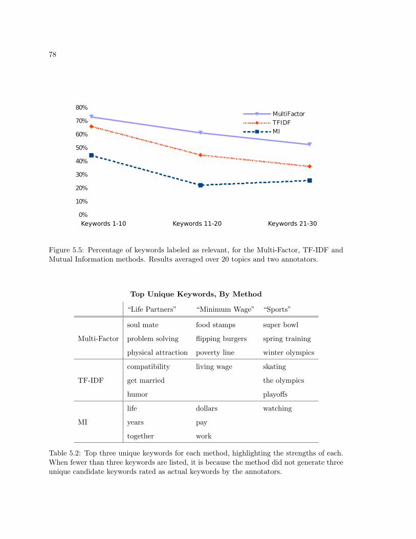
78
0%
10%
20%
30%
40%
50%
60%
70%
80%MultiFactor
TFIDF
MI
Keywords 1-10 Keywords 11-20 Keywords 21-30
Figure 5.5: Percentage of keywords labeled as relevant, for the Multi-Factor, TF-IDF andMutual Information methods. Results averaged over 20 topics and two annotators.
Top Unique Keywords, By Method
“Life Partners” “Minimum Wage” “Sports”
Multi-Factor
soul mate food stamps super bowl
problem solving flipping burgers spring training
physical attraction poverty line winter olympics
TF-IDF
compatibility living wage skating
get married the olympics
humor playoffs
MI
life dollars watching
years pay
together work
Table 5.2: Top three unique keywords for each method, highlighting the strengths of each.When fewer than three keywords are listed, it is because the method did not generate threeunique candidate keywords rated as actual keywords by the annotators.

79
5.3.1 Data and Model
We use a 20 court case transcript subset of the Supreme Court corpus.3 Since these exper-
iments only involve a qualitative discussion, we use a single (training) set, with 207k word
tokens (7.3k word types) from 58 speakers. All speakers are labeled with one of two roles:
justice or attorney. We again use bigrams, and our vocabulary consists of all 7.3k word
types that appeared in the training data.
5.3.2 Discussion
In our trained model, we find topically relevant keywords appearing for the case-dependent
sparse matrices. Examples include:
1. Rush Prudential HMO, Inc. v. Moran. An HMO denying a request to cover a
surgery: “savings clause,” “medical necessity,” “h m,” “m o,” “pilot life.”
2. TRW v. Andrews. Allegations of violating the Fair Credit Reporting Act: “equi-
table estoppel,” “reporting agency,” “misrepresentation exception,” “liability arises.”
3. Harris v. United States. Regarding the sale of illegal narcotics while carrying an
unconcealed firearm: “mandatory minimum,” “reasonable doubt,” “seven years.”
4. Edelman v. Lynchburg College. A claim of discrimination in the denial of tenure
at a college: “under oath,” “title VII,” “common law.”
5. Owasso Independent School Dist. No. 1011 v. Falvo. A claim that peer
grading violates FERPA: “school district,” “tenth circuit,” “grade book,” “education
record.”
6. Toyota Motor Mfg v. Williams. A claim of assembly line work leading to carpal
tunnel syndrome: “worker’s compensation,” “assembly line,” “life activity.”
3www.oyez.org

80
The model also learned characteristic language associated with the roles of justice, in-
cluding question words (“why,” “how,”) and confirmations structured as statements (“you’re
saying,” “your view,” “I thought”), and attorney, including deferential language (“your
honor,” “chief justice,” “that’s correct”) and hedging (“I think”).
The per-speaker factors are most reliable for justices, for whom the data covers several
cases. In this, we captured speaker idiosyncrasies (e.g. Breyer’s habit of starting sentences
with “all right” and Scalia’s disfluencies) and Rehnquist’s expressions that are characteristic
of the role of Chief Justice (e.g. “we’ll hear,” ”minutes remaining,” ”is submitted”).
5.4 English Genre Modeling Experiments
In Sec. 5.2 we showed that the Multi-Factor model can account for variation in topic, and
in Sec. 5.3 we saw that it can account for the overlapping influences of topic, speaker and
role, but in both cases the our data came from a single genre (telephone conversations
and court cases, respectively). In this section we take a brief look into how the Multi-
Factor model handles data coming from heterogeneous genres. We revisit the two television
genres encountered in experiments of Chapter 3, using a small amount of data from the
“broadcast conversations” (BC) genre, which are political and news talk shows that are
largely unscripted discussions or interviews between hosts and guests, and a larger amount
of the more abundant broadcast news (BN) genre, which is mostly scripted and more formal
in tone. The data and vocabulary configuration is the same as in Chapter 3 (the statistics
are repeated for convenience in Tab 5.3). Our vocabulary size is 5k and all OOV tokens are
mapped to a dedicated OOV token. Our Multi-Factor model has four weight matrices: a
general low rank L, a general sparse S, a BC-dependent sparse SBC and a BN-dependent
sparse SBN .
After jointly training, we evaluate on the BC Test set using weights L + S + SBC
(discarding the BN-dependent weights). The results are listed in Tab. 5.4. In contrast
to the interpolated mKN bigram models trained on BC and BN, which uses a held-out
development set to find the optimal interpolation weights, the Multi-Factor has no such
source of supervision guiding the relative importance of the two data sources. Despite
this limitation, it recovers a fair amount of the perplexity obtained by incorporating the BN

81
Dataset Size (words)
BN Train 3.2M
BC Train 99K
BC Dev 189K
BC Test 136K
Table 5.3: Multi-Factor genre modeling experiment data.
Model Test Set Perplexity
mKN BC-only 166.7
Multi-Factor (L+ S + SBC) 118.5
mKN BC + mKN BN 82.6
Table 5.4: Multi-Factor genre modeling experiment results.
data. Ideally, the method would be able to permit more control over the relative importance
the model gives to different portions of the data to permit it to beat the 82.6 perplexity
number. Extensions to permit control over the relative importance of particular subsets of
the data is an important future direction.
In Tab. 5.5, we take a look at what the SBC and SBN matrices are learning. The top
15 positive exceptional bigrams are listed for BC and BN. The initial observation is that
it appears to be modeling the topical differences between the two data associated with the
two genres more so than the actual genre differences themselves. However, some genre
phenomena do appear; for example, the presence of “the” in the BN list does appear to be
capturing a true genre difference, since the relative frequency of the word “the” is roughly
10% lower in BC than BN.
In Tab. 5.6 we list the exceptions we deem to be indicative of spontaneous, conversational
speech among the top 200 exceptions for BC and for BN. In this case, more genre differences
are evident. BC shows, which often involve discussion of personal positions on issues,
include phrases reflective of this interaction, such as “ya know,” “i wanna,” and “yea.”

82
Given the frequency of contention in BC shows, it is not surprising that they also show
disfluencies associated with holding the floor, like “um” and “uh.” Whereas in BC, with
mostly in-studio discussions where nodding and other non-verbal back-channels are possible,
the interaction between in-studio anchors and remote reporters in BN is more similar to
telephone interaction, with verbal backchannels like “uh-huh” and phrases like “bye bye”
at the end of conversations.
Despite this evidence that some genre phenomena are being captured, the emphasis of
topical phrases in the lists suggests a straightforward extension of the Multi-Factor model,
where one is not limited to modeling the influence of different factors as sparse corrections,
but as low rank corrections (instead or in addition to the sparse corrections). Such a
structure would likely be better able to handle the systematic rather than sparse nature of
language usage differences between genres. While this extension can be handled with minor
variants of modeling framework and training algorithms already introduced, we leave the
assessment of such an extension to future work.
5.5 Conclusions
In summary, we introduced a multi-factor exponential language model that allows super-
vised learning of overlapping factors that influence sequential language behavior. As a
language model, the model provides small gains in perplexity in a topic adaptation scenario
compared to a baseline modified-Kneser-Ney that interpolates general and topic specific
models. It can also be used as a mechanism to identify factor-dependent characteristics.
In particular, the n-gram elements encoded in sparse parameter matrices give an intuitive
way to identify factor-dependent keyword phrases. On a conversational speech task, we
demonstrate that human raters prefer topic keywords learned by the multi-factor model
over TF-IDF and mutual information baselines. With Supreme Court transcripts, we show
qualitatively the ability to learn factor-dependent keywords for different court cases, roles
(justice vs attorney), and speakers. Experiments modeling heterogeneous genres show some
promising initial perplexity results, but suggest that low-rank corrections may be useful in
addition to (or possibly instead of) the sparse correction structure when the differences are
systematic rather than exceptional. In addition to summarization, identification of keyword

83
BC Exceptions BN Exceptions
san francisco los angeles
hum v’s et cetera
thelma wahl al qaeda
neil entwistle bin laden
al queda bin laden’s
mike gowan abu ghraib
leslie ballin the
patricia whitfield abu musab
robert bork cnn com
chicken hawk dianne feinstein
mary kero sharm el
bob woodruf al qaida
representative kilmartin aneesh raman
micah garen keith oppenheim
emile lahoud sherrod brown
Table 5.5: Top 15 bigram exceptions in the BC and BN matrices.
BC Spontaneous Exceptions BN Spontaneous Exceptions
ya know ha ha
mhm uh huh
i wanna bye bye
uh whoa whoa
eh eh
lets lets
yea
um
Table 5.6: Bigram exceptions indicative of spontaneous, conversational speech data foundamong the top 200 BC and BN exceptions.

84
phrases is of interest for feature selection, learning lexical items (as shown in Chapter 4), and
detecting new events by learning keywords on new data sources. Encoding words with other
features (e.g. morphological structure, syntactic dependents) would also make it possible
to identify other types of idiosyncratic phenomena.

85
Chapter 6
MODEL EXTENSIONS
This thesis has focused on the task of modeling the probability of a sequence of cate-
gorical symbols, p(x1, x2, . . . , xT ); in particular, on the language modeling case where the
symbols are words. We also explored how byproducts of our model, such as sparse matrix
entries, could be useful for other language processing tasks. However, the low rank ideas
developed here can be easily translated to other modeling problems. In this chapter we will
introduce the models and algorithms for two important extensions: first, to the sequence
tagging problem and second to the acoustic modeling problem. The goal here is to show
that the techniques developed are broader than language modeling; we leave experimental
evaluation to future work.
6.1 Sequence Tagging
The problem of sequence tagging is closely related to the language modeling problem studied
extensively in this thesis. In tagging, there are two parallel sequences: x1, . . . , xT and
y1, . . . , yT . For example, xi may denote the i-th character in a word, while yi denotes its
corresponding pronunciation (possibly null if not pronounced). Often the goal is to predict
the sequence of labels y1, . . . , yT from some sequence of observations x1, . . . , xT . This can
be accomplished either by modeling the joint distribution P (x1, . . . , xT , y1, . . . , yT ), or by
modeling the conditional distribution p(y1, . . . , yT |x1, . . . , xT ) = p(y|x) directly, where we
will use bold lowercase letters to denote sequences. Clearly, this is a more challenging task:
there are potential interactions between y’s, between x’s, and between y’s and x’s. As in
language modeling, conditional independence assumptions are often made to control model
complexity.

86
...
Y1
Y2
Y3
YT-1
YT
X1, X
2, … X
T
Figure 6.1: A graphical representation of the conditional independence assumptions in thefirst-order linear chain conditional random field.
6.1.1 The Low Rank Conditional Random Field
Two different models are popular in the field of language processing for sequence tagging:
hidden Markov models and conditional random fields (CRFs). The feature-based approach
of the exponential models introduced in Chapter 4 is most naturally incorporated into the
CRF, so it will be our focus. If we assume that the label sequence is a first-order chain, we
obtain the linear chain CRF, which is defined to be:
p(y|x) =∏ni=1 exp(θ
T f(yi−1, yi, x))∑
y′
∏ni=1 exp(θ
T f(y′i−1, y′i, x))
. (6.1)
The conditional independence assumptions of this undirected graph are shown in Fig. 6.1;
the basic assumption is that the probability can be decomposed into potentials over pairs
of adjacent words and the entire input sequence x. Feature function f maps to Rd, and
the model is parameterized by a weight vector θ ∈ Rd. In a higher-order (nth-order) linear
chain CRF, is
p(y|x) =∏ni=1 exp(θ
T f(yi−n, . . . , yi, x))∑
y′
∏ni=1 exp(θ
T f(y′i−n, . . . , y′i, x))
. (6.2)
The primary complication of moving to larger orders is in inference, which is needed both
to make predictions and during parameter estimation. Exact inference is quadratic in the
size of the label alphabet for linear chain CRFs, and quartic in the size of the label alphabet
for second-order chain CRFs. We focus our discussion on first order models for notational
simplicity.
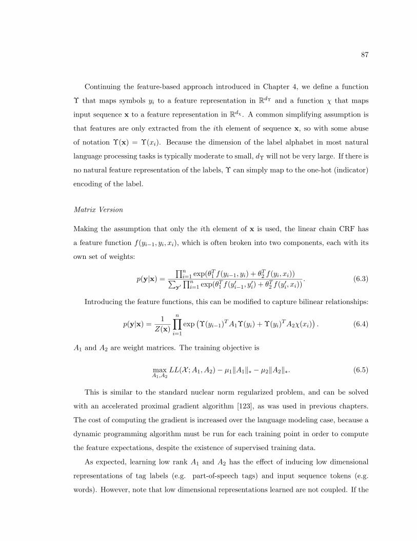
87
Continuing the feature-based approach introduced in Chapter 4, we define a function
Υ that maps symbols yi to a feature representation in RdΥ and a function χ that maps
input sequence x to a feature representation in Rdχ . A common simplifying assumption is
that features are only extracted from the ith element of sequence x, so with some abuse
of notation Υ(x) = Υ(xi). Because the dimension of the label alphabet in most natural
language processing tasks is typically moderate to small, dΥ will not be very large. If there is
no natural feature representation of the labels, Υ can simply map to the one-hot (indicator)
encoding of the label.
Matrix Version
Making the assumption that only the ith element of x is used, the linear chain CRF has
a feature function f(yi−1, yi, xi), which is often broken into two components, each with its
own set of weights:
p(y|x) =∏ni=1 exp(θ
T1 f(yi−1, yi) + θT2 f(yi, xi))
∑
y′
∏ni=1 exp(θ
T1 f(y
′i−1, y
′i) + θT2 f(y
′i, xi))
. (6.3)
Introducing the feature functions, this can be modified to capture bilinear relationships:
p(y|x) = 1
Z(x)
n∏
i=1
exp(
Υ(yi−1)TA1Υ(yi) + Υ(yi)
TA2χ(xi))
. (6.4)
A1 and A2 are weight matrices. The training objective is
maxA1,A2
LL(X ;A1, A2)− µ1‖A1‖∗ − µ2‖A2‖∗. (6.5)
This is similar to the standard nuclear norm regularized problem, and can be solved
with an accelerated proximal gradient algorithm [123], as was used in previous chapters.
The cost of computing the gradient is increased over the language modeling case, because a
dynamic programming algorithm must be run for each training point in order to compute
the feature expectations, despite the existence of supervised training data.
As expected, learning low rank A1 and A2 has the effect of inducing low dimensional
representations of tag labels (e.g. part-of-speech tags) and input sequence tokens (e.g.
words). However, note that low dimensional representations learned are not coupled. If the

88
optimal A1 = U1VT1 and A2 = U2V
T2 , then the three maps from label sequence y to low-
dimensional representations, UT1 , VT1 and UT2 , need not be the same. Indeed, UT1 and UT2
need not map to the same lower dimension. This is (at least partially) desirable behavior.
If UT1 and V T1 were coupled, it would favor sequences that repeated labels. Constraining UT1
to be near UT2 assumes that the same mapping preserves the discriminative information for
both potential functions (between pairs of labels and between labels and input elements),
and that the optimal lower dimension is the same, either of which may or may not be true.
Depending on the nature of the problem, it may also be of interest to frame the weights
as sparse plus low rank, so that Ai = Si + Li. The problem remains convex, and could be
handled using the same optimization techniques applied in Chapters 4 and 5.
Tensor Version
While the matrix variant captures two pair-wise relationships with two bilinear structures
(matrices), one can also directly capture multi-way relationships directly with a multilinear
structure (tensor). There are a few natural ways to approach this. First, in the linear chain
CRF discussed above, the function f(yi−1, yi, x) need not be broken into two, but instead
modeled multilinearly. This gives a model of the form
p(y|x) = 1
Z(x)
n∏
i=1
exp (A×1 Υ(yi−1)×2 Υ(yi)×3 χ(x)) . (6.6)
Recall from Chapter 2 that tensor multiplication generalizes matrix multiplication: A×i zdenotes multiplying vector z along the i-th mode of a tensor A. Generalizing the above
model to an m-order Markov assumption on the labels yields
p(y|x) = 1
Z(x)
n∏
i=1
exp (A×1 Υ(yi−m)×2 Υ(yi−m+1)×3 · · · ×m+1 Υ(yi)×m+2 χ(x)) . (6.7)
Either of the above models can be solved with the CMLE algorithm [112], optimizing
the non-smooth, convex objective:
minA‖A‖∗ − LL(X ;A). (6.8)
Because this approach has greater time complexity than the problems discussed in previous
chapters, steps must be taken to keep the feature dimensions and tensor order down (e.g.,

89
by projecting large feature representations to lower dimensional space before training the
model).
6.1.2 Summary
In this thesis, we have seen how sequences of symbols (typically words) can be modeled
with bilinear and multilinear models, and how the notions of matrix rank and sparsity can
give rise to models that are both easy to train and easy to interpret. The sequence tagging
problem takes this one step further: again we are determining probabilities of a sequence y,
but in this case we also condition on a separate sequence x whose information is critical to
determining y’s probability. Compared to the language model introduced in Chapter 4, the
conditional random field discussed here has two key differences. First, we need to normalize
over entire sequences, rather than just the next symbol. This only affects the log-probability
and can be addressed with dynamic programming in a standard way. The second is that
the need arises to model general multilinear relationships (as opposed to the history-word
bilinear relationship). This is accomplished by replacing matrix weights with tensor weights,
and replacing the matrix nuclear norm to encourage low matrix rank with the tensor nuclear
norm to encourage low tensor n-rank. Like a low rank matrix, a low n-rank tensor induces
low-dimensional representations of the objects it is modeling. Conveniently, training these
proposed tagging models involves solving convex optimization problems for which suitable
algorithms already exist.
6.2 Acoustic Modeling
An acoustic model describes the probabilistic relationship P (o1, . . . , oT |s1, . . . , sT ) betweenan acoustic observation sequence o1, . . . , oT and the corresponding latent linguistic state
sequence s1, . . . , sT that produced it.1 We focus in particular on the state-dependent emis-
sion distributions, p(o|s), which are typically Gaussian mixture models. Each state models
the acoustic characteristics of a portion of a context-dependent phone. Research has shown
1Typically in speech recognition the problem is phrased as giving the probability of acoustic observationgiven a word sequence, but ultimately the word sequence must be mapped to a state sequence; e.g., witha pronunciation dictionary mapping words to a sequence of individual context-dependent phone models.

90
that context-dependency improves performance because it better models phenomena like
coarticulation, but there are limits to the context that can be accounted for. With a pho-
netic inventory of 50 and three states per context-dependent phone, there are 375k possible
triphones or 937.5M possible quinphones. Clearly, no reasonable amount of training data
supports training such a large number of context-dependent models. Training each of these
models can be seen as solving related sub-problems, which suggests that we should solve
them jointly. The dominant strategy of explicitly tying models using a decision tree which
partitions the tri- or quinphone set by asking questions about the left and right context is
interpretable and effective, but it relies on knowledge of the target language for designing
possible questions. A more recent technique for training models jointly is known as the
Subspace Gaussian Mixture Model [97], in which a large set of mixtures are shared among
all states, but the mean vectors are distinct for each state, living in a subspace of possible
mean vectors. We propose here a general, principled approach, where shared, continuous
representation of phones and contexts are learned and used to solve each of the individual
context-dependent phone modeling problems jointly.
Specifically, we will propose a new approach to acoustic modeling, in which multilinear
relationships between the acoustics, phone, context and states are learned, and the complex-
ity is controlled by the n-rank of a weight tensor. This not only gives us control over model
complexity, but as a byproduct learns a low-dimensional representation of the acoustics, the
phone, the context and the state. It then is capable of defining distinct (but multilinearly
related) distributions for all possible tri- or quin-phone states. We will show that it can be
used directly as an acoustic model, as a mechanism to learn feature transformations and
as a way to partition the space of context-dependent phones, allowing it to be used as a
clustering method in traditional acoustic models.
6.2.1 The Low n-Rank Tensor Acoustic Model
The dominant approach to speech recognition uses a Hidden Markov model with Gaussian
mixture models for the output distributions. However, one can plug in a different output
distribution; this is commonly referred to as a “hybrid” approach. Hybrid approaches

91
typically involve a discriminative state posterior model p(s|o) and Bayes’ rule:
p(o|s) = p(s|o)p(o)p(s)
(6.9)
The maximum likelihood estimate of the denominator p(s) can be obtained trivially from
an initial alignment. The p(o) term can be ignored during decoding (i.e. finding the most
probable state sequence), since it is a non-negative constant. Thus the focus is on the state
posterior model, p(s|o).
Although neural networks are the most famous example for p(s|o) in hybrid automatic
speech recognition (ASR), one can use any model that produces valid probabilities, including
a maximum entropy model. In this case, the state posterior probabilities are given by:
p(s|a) = exp(wTs a)∑
s′ exp(wTs′a)
. (6.10)
Here s ∈ 1, 2, . . . , C is the state index, ws ∈ RD is a state-dependent weight vector and
a ∈ RD is the acoustic feature vector. An example of an approach similar to this is presented
in [52], where phone classification performance was comparable to many published results,
but not state-of-the-art. One obvious way to extend the above model is to incorporate
second order features, replacing the state-dependent weight vectors with weight matrices:
p(s|a) = exp(aTWsa)∑
s′ exp(aTWs′a)
. (6.11)
This is equivalent to Eqn. 6.10 where a contains all pairs of products between the frame’s
acoustic feature elements (along with the original features themselves), and is a standard way
to improve linear discriminability between classes. Note that our overall set of parameters
is a tensor W, where each Ws is just a matrix slice of W. If we let z denote an indicator
vector of the state s, we get the same equations in a different form:
p(s|a) = exp(W ×1 a×2 a×3 z)∑
z′ exp(W ×1 a×2 a×3 z′)=
exp(∑
i,j,k aiajzkWijk)∑
z′ exp(∑
i,j aiajz′Wijk)
. (6.12)
The problem with this parameterization is that there can be too many free parameters,
and there is no inherent tying between states. This is remedied by imposing a structure
on W; namely, making it have low n-rank. Recall that the n-rank of a tensor is a tuple

92
of scalars, one for each mode. If W has n-rank < r1, r2, r3 >, then there exist matrices
U1 ∈ RD×r1 , U2 ∈ R
D×r2 and U3 ∈ RC×r3 and a core tensor G ∈ R
r1×r2×r3 such that
p(s|a) = exp(W ×1 a×2 a×3 z)∑
z′ exp(W ×1 a×2 a×3 z′)=
exp(G ×1 (UT1 a)×2 (U
T2 a)×3 (U
T3 z))
∑
z′ exp(G ×1 (UT1 a)×2 (UT2 a)×3 (UT3 z′)).
(6.13)
This has the following interpretation: rather than model the second order features of the
input directly, we first learn two linear transformations of the acoustic features, U1 and U2
that project a down to r1 and r2 dimensional representations, and then model the second
order features of those lower-dimensional features (preliminary experiments suggest that,
as expected, U1 = U2 due to the symmetry of the problem setup). Further, we learn a low
dimensional representation of the state, UT3 z, so the weight matrix for state s is a linear
combination of r3 basis matrices (UT3 z are the mixture weights). This gives a mechanism
to exploit similarities between states.
We can go even further, though, by using a factored representation of the state. Rather
than have a single state indicator vector z, say we could have three indicator functions,
ΦC(s), ΦL(s) and ΦR(s) that map a state s to its center phone identity and left and right
phone contexts, respectively. If we let W be the corresponding fifth-order tensor, then we
obtain the following acoustic model:
p(s|a) =exp(W ×1 a×2 a×3 Φ(s)
C ×4 ΦL(s)×5 Φ
R(s))∑
s exp(W ×1 a×2 a×3 ΦC(s′)×4 ΦL(s′)×5 ΦR(s′))(6.14)
=exp(
∑
i,j,k,ℓ,m aiajΦCk (s)Φ
Lℓ (s)Φ
Rm(s)Wijkℓm)
∑
s′ exp(∑
i,j,k,ℓ,m aiajΦCk (s
′)ΦLℓ (s′)ΦRm(s
′)Wijkℓm). (6.15)
Assuming the state labels are obtained via a forced alignment from an HMM-GMM
system, there will be a limited number of state labels, so the sum in the denominator of
Eqn. 6.15 is over the same set of states as in Eqn. 6.13. But when we regularize W to
be low weight we now learn five basis matrices, U1, U2, . . . , U5. As before U1 and U2 are
transformations of the acoustic features a (and should be equal), while U3 now gives a low
dimensional representation of the center phone, U4 gives a low dimensional representation
of the left context phone and U5 gives a low dimensional representation of the right context
phone. For notational simplicity we do not explicitly include the phonetic state index, or

93
other potentially useful factors like tone in tonal languages. Those can be included either
by expanding the order of the tensor, or by creating distinct indicator entries for different
state or tone labels. Quinphone models are a straightforward generalization of triphone
models. Factoring the representation has a few key benefits:
• The weight tensor allows all possible triphones to be covered, and due to the smoothing
effect of the n-rank regularization, the model can will learn non-zero probabilities for
all triphones. For practical speed considerations during training, one may restrict the
support to cover only the triphones observed in the training data and normalize over
only this subset of triphones. At run-time, any set of triphones can be accommodated
simply by changing the normalization term.
• We can use the low dimensional representations to cluster the center phone and left and
right context phones, yielding a similar effect as decision tree state tying. This allows
the weights learned in our model to be injected back into a standard HMM-GMM,
which may be desirable for practical reasons (e.g. using standard, well-optimized
tools). It may also benefit other discriminative acoustic models (e.g. deep neural
networks), whose triphone state inventory typically comes from a baseline HMM-
GMM system. Earlier work [37] showed clearly that using context-dependent phone
states as opposed to context-independent ones improves deep neural network acoustic
modeling performance; it is possible that better triphone state sets could provide
additional benefit.
6.2.2 Training
With or without a factored representation of the state, the model can be trained by solving
a non-smooth convex optimization problem:
minW‖W‖∗ − LL(X ;W). (6.16)
LL is the average log-likelihood of the data ( 1N
∑Ni=1 p(si|ai)) and ‖ · ‖∗ denotes the convex
tensor nuclear norm. It can be solved using the Convex Multilinear Estimation algorithm
[112].

94
6.2.3 Computational Complexity
The primary limitations of this approach are the time complexity (one singular value de-
composition is required for each mode of the tensor at each iteration) and the memory
complexity (one needs to be able to hold a full-rank, dense tensor in memory). To give a
sense of the computational costs, we consider two scenarios with typical placeholder values,
the first does not factor state representation, while the second does.
• Non-factored state. If we use the non-factored triphones, with 5000 triphone phone
states, and our acoustic features are the second order features of the concatenation of
seven frames of 13-dimensional mel frequency cepstral coefficients, the tensor contains
5000(13 · 7)2 ≈ 41M elements and uses roughly 0.33 GB of memory (assuming double
precision). Three SVDs would need to be computed at each iteration (two acoustic
feature modes and one state label mode), two on matrices of dimension 91 × 455000
and one on a matrix of dimension 5000 × 8281. The first would be fairly fast and
the last not prohibitive (we have no trouble with matrices larger than that in the
SLR-LM).
• Factored state. Using the same second order acoustic features, but instead using a
factored representation of the triphone state, with a phone inventory of 40 and 3
states per phone, the tensor would contain 3 ·403(13 ·7)2 ≈ 1.6B elements, and require
12.7GB to store. Now six SVDs would be required per iteration (one state mode, three
phone modes and two acoustic feature modes). The first matrix would be dimension
3 × 530M, the next three dimension 40 × 39.7M and last two dimension 91 × 17.5M.
Due to the extreme asymmetry in the dimensions, the SVD computation costs are
surprising light. (Recall that the SVD has linear cost in the larger dimension and
quadratic cost in the smaller dimension).
6.2.4 Conclusions
Acoustic modeling is a challenging problem that requires trade-offs between accuracy and
trainability. The literature clearly indicates that context-dependent modeling improves

95
performance, but this comes at a cost. If there are K phones, then a context-dependent
acoustic model is tasked with assigning an emission distribution to K3 triphones (or K5
quinphones). Viewing the training of each context-dependent model as a sub-problem to
solve, one observes that there are many ways in which the sub-problems are related. Intu-
itively, context-dependent phones sharing a common center phone should have some under-
lying commonalities, but to a lesser extent, so should those sharing the same left or right
contexts. The traditional strategy of clustering context-dependent phones can be viewed
(like n-gram back-off) as a rigid mechanism for solving related problems jointly. In that
case, sub-problems are either merged entirely or left completely distinct. We propose here
a a more flexible way to exploit the commonalities, by phrasing the training problem as
estimating a low n-rank tensor which learns a shared representation of the acoustics and
the state. Conveniently, the joint training problem is convex, and algorithms exist to solve
it.
Besides providing state posterior probabilities for use in hybrid ASR, our model has
other potential applications. The low-dimensional representations it learns can be used to
cluster triphones (or quinphones), which can improve traditional HMM-GMM systems (at
the least, it removes the need for linguistic knowledge when determining state tying), but
can also provide better targets for other state-of-the-art discriminative acoustic models (e.g.
deep neural nets) whose triphone state inventory often comes from a baseline HMM-GMM.
It is completely compatible with the “tandem” ASR approach, whereby state posteriors are
used as features (typically after another dimensionality reducing transformation). Finally,
the acoustic feature transformations learned by the model may be useful themselves as a
data pre-processing stage, since by design they preserve information that is discriminative
when a model makes use of their second order features (as is the case in a full covariance
GMM).

96
Chapter 7
SUMMARY AND FUTURE DIRECTIONS
7.1 Summary of Contributions
7.1.1 New Modeling Frameworks and Experimental Findings
Many fundamental language processing problems have a vast ambient dimension, requir-
ing the use of simplifying assumptions when building models of language. The primary
example in this thesis is the assigning probabilities to sequences of categorical variables,
p(x1, x2, . . . , xT ), whose joint probability table has vT entries (where v is the size of the
vocabulary from which the variables are drawn). Standard non-parametric maximum likeli-
hood estimates of this table are plagued with zero probability estimates, and thus very poor
for use in real applications. Fortunately, there is a great deal of regularity in language, so
that its intrinsic dimension is much lower. Different simplifying assumptions can be viewed
as different ways to capture the intrinsic variability in language - that is, identify the mean-
ingful patterns without fitting the noise in a finite training sample. In this thesis we develop
a new way to view the sequence modeling problem, which has two key components:
1. We parametrize our models with matrices or tensors to capture bilinear or multilinear
relationships between symbols, increasing the expressiveness of our model relative to
standard models.
2. We regularize the matrices or tensors to be low rank, sparse, or the sum of the two
structures. This yields highly interpretable models. The low rank weights can be
seen as finding one or more low-dimensional subspaces that capture the meaningful
variation in language, and more directly tackles the goal of uncovering the intrinsic
dimension in the high ambient dimension problem. They typically induce continuous
low-dimensional representations of words, giving us geometric intuition into the rela-
tionships between words. We also observe that sparse weights nicely complement the

97
low-rank weights, distinguishing exceptional patterns from regular ones.
These characteristics are embodied in three new language models, evaluated under many
experimental conditions. In Chapter 3, we introduce a novel factored low rank tensor lan-
guage model, termed the Low Rank Language Model (LRLM), which is motivated by the
observation that most existing language model smoothing techniques have the effect of re-
ducing the rank of conditional probability tables. The LRLM models the joint probability
over n-grams directly as a tensor and then constrains the tensor rank. This can be in-
terpreted as learning a mixture of position-dependent unigram models, where the number
of mixtures is equal to the tensor rank. We observe that it improves perplexity over the
popular, widely-used modified Kneser-Ney n-gram model in a limited-data scenario. We
also draw connections between low rank tensor language modeling and related problems,
including non-negative tensor factorization.
In Chapter 4, the rank regularization idea is extended into the exponential language
model framework, penalizing the rank of a weight matrix rather than the probabilities
themselves, which is the fundamental difference relative to LRLM of Chapter 3. The model,
termed the Sparse Plus Low Rank Language Model (SLR-LM), gives probabilities p(x|h)of words x given histories h, and the weight matrix defines a bilinear function of word and
history features. In doing so, we observe that learning a rank r weight matrix is equivalent
to learning r-dimensional continuous representations of words and histories. In contrast
to Latent Semantic Analysis, neural network language models and other continuous-space
techniques, the rank and thus dimensionality r is learned during training, instead of being
fixed ahead of time. One important finding of this work was that rather than using a low
rank weight matrix alone, it is better to parameterize the model with the sum of two matri-
ces: the low rank matrix and a sparse matrix. The latter “corrects” the former, increasing
or decreasing n-gram probabilities due to exceptional linguistic behavior (e.g. to correct for
multiwords like “united states”). We extensively evaluate the SLR-LM, including language
modeling experiments in English, Cantonese, Pashto, Turkish, Tagalog and Vietnamese,
finding consistent perplexity reductions of 5-9% over a modified-Kneser-Ney baseline. Tak-
ing advantage of the flexibility afforded by the feature functions, the chapter includes ex-

98
perimental results using morphological features in Turkish, a morphologically-rich language,
where we find that we can improve perplexity over a word-feature-based SLR-LM. Finally,
we introduce a new technique for the automatic identification of words and multiwords, us-
ing the entries of the sparse matrix, and evaluate it on character-segmented Cantonese data
and syllable-segmented Vietnamese data. We find that we can obtain small improvements
in perplexity using the learned words, and obtain larger gains in the dictionary precision
rates.
In Chapter 5, we extend the SLR-LM to be able to account for overlapping influence
on language behavior, including the topic, genre, speaker or author identity, role, etc. This
extension, termed the Multi-Factor SLR-LM, replaces the single sparse matrix with a set of
sparse matrices, one dedicated to each possible influence. Factoring the model in this way
has two key advantages: first, it allows us to identify the words or phrases most important
to a given topic, genre, etc., and second, it provides a new method for model adaptation
(e.g. certain weights can be kept as is, others can be discarded, and others learned new).
We evaluate both on English conversational telephone data, focusing on accounting for
variation in topic. We see small gains in perplexity and larger gains in topic keyword
precision. We also present a qualitative analysis on a Supreme Court transcript case to
explore the potential for capturing more than one type of factor and see that meaningful
phrases for speakers, roles and court cases are being learned. Finally, we evaluate the ability
to model heterogeneous genres on English broadcast news and broadcast conversation data.
Some genre phenomena are captured, but the results motivate an extension of the Multi-
Factor model that permits factors to be modeled with low rank corrections, to be left for
future work.
Although our focus is on language modeling, in Chapter 6, we introduce new models
and training algorithms that extend our approach to two other important human language
processing tasks. Our first extension generalizes our sparse plus low rank sequence model to
the sequence tagging task, where we need to assign probabilities to one (label) sequence given
a second sequence. To do this, we need to extend the bilinear relationships we modeled with
matrices to multilinear relationships modeled with tensors. Our second extension branches
out into the task of acoustic modeling, where we introduce several ways in which we can

99
use low n-rank tensors to find posterior probabilities over context-dependent phone states
given an acoustic feature input.
7.1.2 Specific Contributions
The specific contributions of this thesis are:
• The introduction of the novel factored tensor Low Rank Language Model (LRLM)
and the implementation of its learning algorithm, and the interpretation of the LRLM
as a mixture of unigrams, drawing a connection to non-negative tensor factorization.
• The introduction of the novel exponential Sparse Plus Low Rank Language Model
(SLR-LM) and the implementation of its learning algorithm and lattice rescoring.
• A multi-language evaluation of the SLR-LM, including results on English, Cantonese,
Pashto, Turkish, Tagalog and Vietnamese.
• A study of the use of morphological features in the SLR-LM on Turkish data, finding
that perplexity improvements can be obtained on a morphologically rich language over
a word-only SLR-LM.
• A novel method for finding words and multiwords using the sparse entries of a SLR-
LM, and a study of its effectiveness on character-segmented Cantonese and syllable-
segmented Vietnamese, in terms of its ability to discover dictionary words and its
ability to lower language model perplexity through data resegmentation.
• The introduction of the novel exponential Multi-Factor SLR-LM, which uses super-
vised training to factor the effects of an arbitrary number of overlapping factors (e.g.
topic, genre, speaker) and the implementation of its learning algorithm.
• A novel method for keyword extraction, using the sparse entries of a Multi-Factor
SLR-LM, and a study of topic keywords in English.
• A novel method for language model adaptation using the Multi-Factor SLR-LM.

100
• A modeling and algorithmic guide for extending the low rank sequence modeling
techniques to sequence tagging and acoustic modeling applications.
7.2 Future Directions
There are several promising future directions that build on the work in this thesis. We
discuss them here in terms of three categories: algorithm and computational improvements,
extensions to our language modeling approach, and novel models for new applications.
7.2.1 Algorithmic and Computational
New, sophisticated models often come with a computational cost, and the SLR-LM and
its variants are no exception. There are two training bottlenecks, itemized below, with the
following potential work-arounds:
1. Storing the weight matrices and computing the singular value decomposition (SVD).
In our algorithms, the gradients are typically dense and full rank, so they cannot be
represented in a compact form and require dφdψ entries. Computing the SVD then
requires dψdφr operations, where r is the current estimate of the rank. The easiest
way to address both the memory and computational problems is to limit the size of the
vocabulary and to limit the n-gram order (thus reducing the dimension of the history
features), but alternative encoding strategies could also be employed to reduce the
dimensions. Chapter 4 introduced two such options: using a morphological feature
representation of words and using a “bag-of-x” representation for histories. Rather
than indicator encodings of words and histories, one could also start with moderate-
dimensional continuous representations learned elsewhere; for example, from a previ-
ously trained lower-order or smaller vocabulary SLR-LM. The primary disadvantage
of starting with a continuous representation is that it would come at the cost of inter-
pretability of the sparse matrix, whose entries would no longer represent n-grams. To
deal with dψ in particular, one strategy would be to limit the vocabulary’s size by ex-
cluding infrequent words, and design the model to be interpolated with or backoff to a
full vocabulary n-gram model, as has been done before with neural network language

101
models. Another strategy would be to use word classes, as is done in Model M and
in newer neural network language models. Regarding the SVD itself, we have done
some preliminary exploration of SVD speedups using approximate and randomized
algorithms [50, 43, 82], observing a small degradation in performance, but we have
not tested this systematically. Another possibility for SVD speed-up is to use the
“warmstarted” SVD [130], which does not start the SVD computation from scratch,
but is instead seeded with the result from a previous iteration. This approach seems
promising, but remains unexplored in our experiments.
2. Computing the gradient. Ultimately, HV conditional probabilities must be computed
in order to compute the full gradient, where H is the number of unique histories
observed in the training data and V is the vocabulary size. We have implemented
and informally explored the use of stochastic mini-batch gradients, where a subset
of the histories are sampled and all n-grams with those histories are used in train-
ing. When the histories are weighted by the n-gram counts to favor more frequent
histories, the method appears to give large memory savings at the expense of some
minor degradation in perplexity. Another approach would be to parallelize full gra-
dient computation over multiple machines, as opposed to multiple local cores as is
currently done. Parallelization over multiple machines would also help to alleviate the
memory costs incurred when H and/or V are large.
Finally, we have relied upon variants of accelerated proximal gradient descent algorithms
to solve our optimization problems. Although these algorithms have optimal theoretical
convergence rates for the general class to which our problems belong, it is conceivable that
the special structure of this problem could be exploited to obtain a better rate. Even if not,
future advances in algorithms may offer speed improvements by a constant factor, or even
better, may be able to reduce the memory complexity of model training.
7.2.2 Modeling Extensions
One very straightforward extension would be to port the idea of a sparse plus low rank
form from Chapter 4 into the factored tensor model of Chapter 3. In this case, the sparse

102
elements would be corrections to the joint probability distribution directly. Although this
would likely benefit the modeling power, it would also complicate training, which is already
problematic due to the non-convexity of the problem. Given these challenges for training,
we feel that improvements targeting the exponential models of Chapters 4 and 5 are more
likely to provide a gain.
So far our exponential SLR-LM models assume a bilinear relationship between two
objects: the next word x and the history h. One could instead break the single history
apart, in order to give additional importance to the most recent words in the history,
which provide the most predictive information. In this case one would extract separate
representations of the immediate history, and learn interactions between all feature vectors
through a weight tensor, A.Recall that p(x|h) is short-hand for p(xt|x1, . . . , xt−1) for some unspecified t. If one
believes that the most recent m symbols in the history should receive special treatment,
one can define h−i = xt−i for i = 1, . . . ,m, and let the remainder of the history be h =
x1, . . . , xt−m−1. Let p(x|h) now denote p(x|h−1, h−2, . . . , h−m, h). Let A be a (m + 2)-th
order tensor, let Ψ map symbols to RdΨ , Ω map symbols to R
dΩ , and let Φ map sequences
of symbols to RdΦ . One could then introduce a low n-rank tensor version of the SLR-LM
as follows:
pA(x|h) =exp(A×1 Ω(h−1)×2 Ω(h−2) · · · ×m Ω(h−m)×m+1 Φ(h)×m+2 Ψ(x))
∑
x′ exp(A×1 Ω(h−1)×2 Ω(h−2) · · · ×m Ω(h−m)×m+1 Φ(h)×m+2 Ψ(x′))(7.1)
Recall that ×i denotes multiplication along the i-th mode. If tensor A is decomposed into
the sum of two tensors, A = L + S, this directly generalizes the SLR-LM in Chapter 4.
Here, the symbol x is mapped with Ψ instead of ψ, the remaining history h is mapped
with Φ instead of φ, and the new history elements h−i are mapped through a third function
Ω. For simplicity, one could let Ω = Ψ, so that single symbols are mapped the same way,
whether in the history or predictive position.
Training this new model is analogous to the SLR-LM:
minS,L
γ0‖L‖∗ + γ1‖S‖1 − LL(D;S + L) (7.2)
where LL is the data log-likelihood as before, and ‖L‖∗ denotes the tensor nuclear norm of
L. This problem can be solved using the CMLE algorithm of [112].

103
Recall that the tensor nuclear norm is the sum over each mode i of the matrix nuclear
norms of the mode i tensor unfoldings.1 That is, it approximates the minimum∑
i ri such
that the fibers of mode i live in an ri-dimensional subspace. This can also be viewed as
learning globally-optimal feature transformations for Ψ(x), Ω(h−1), . . . ,Ω(h−m) and Φ(h)
simultaneously. If the first mode has n-rank r1, then the first history symbol Ω(h−1) is
implicitly mapped down to an r1-dimensional space. Likewise, if the (m + 1)-th mode has
n-rank rm+1, the vector Ψ(x) is implicitly mapped down to rm+1 dimensional space, and so
forth. Instead of a simple inner product between the low-dimensional representations, they
are combined via tensor multiplication with a full rank core tensor, C ∈ R×m+2i=1 ri . The core
tensor encodes the interactions between modes, allowing it to capture more sophisticated
sequence information than the SLR-LM alone.
The price to be paid for the richer modeling abilities would be in terms of time and space
complexity. Training the model would involve unfoldings along each mode, followed by an
SVD on each unfolding. Because unfolding does not efficiently represent the low rank tensor
structure, a compact representation of the matrices is not immediately apparent. Storing
each matrix requires memory linear in the size of the tensor, O(dmΩ dΨdΦ), and computing
the SVD for the i-th mode requires O(dmΩ dΨdΦri) time. The obvious solution is to limit the
size of m, dΨ, dΦ and dΩ. It is expected that a small m (e.g. 1 or 2) should be sufficient,
because 1) most of the key information in language is contained in bigrams and trigrams,
and 2) the remainder of the history still appears in the h term. The cost of the large ambient
feature dimensions may be addressed with the techniques discussed in Sec. 7.2.1.
One final promising direction of this research is to extend our ideas into new modeling
problems beyond sequence modeling. Chapter 6 outlines two such extensions in detail. In
the first, we generalize the low n-rank exponential tensor language model idea sketched above
to the task of sequence tagging, where multilinear relationships are defined not just between
symbols in a single sequence, but between symbols in two sequences. Regularizing the weight
tensor n-rank would have the effect of learning continuous, low-dimensional representations
of each of the symbols involved in the multilinear relationship. The second extension is to
1There exist other definitions of the tensor nuclear norm, but we use this one, defined in Chapter 2,throughout.

104
the realm of acoustic modeling. Here a multilinear relationship is defined between acoustic
features and (a potentially structured representation of) a context-dependent phone state
label, and regularizing the n-rank of the weight tensor induces low-dimensional continuous
representations of the acoustics and of the phonetic state.
7.2.3 New Applications
One natural application direction for our language models is use in automatic speech recog-
nition. As designed, our models can be used in the second pass (lattice rescoring), but are
not practical for first pass decoding. Despite our models’ intrinsic low-dimension, they fac-
tor in a way that is not compatible with “ARPA” style (back-off) n-gram language models,
which are used in many speech recognition systems. This limitation is not unique to our
models: it is shared by neural network models (including deep and recurrent models) and
by some exponential models. Recently, researchers have introduced a strategy for building
ARPA-style models from neural network language models [5]. A similar strategy should
be applicable to our models. Using our language models in a first pass rather than second
pass would improve its ability to make a meaningful impact on speech recognition perfor-
mance. Whether via decoding or through lattice rescoring, the use of our language models
in automatic speech recognition deserves a careful study.
There are additional interesting applications that make use of the interpretability of
the weight structure. For example, in [88], Mikolov et al. find that the low dimensional
continuous word representations learned by recurrent neural network language models very
effectively encode syntactic and semantic regularities. Relations such as male/female are
associated with a specific vector offset; e.g., using the representations of “king” - “man” +
“woman” gives a vector close to the representation of “queen.” They exploit this property to
obtain state of the art performance on the SemEval-2012Measuring Relation Similarity task.
Given that the log-bilinear model to which our models are most closely related obtains very
strong performance, it would be interesting to evaluate the low dimensional representations
learned by the SLR-LM for this same purpose.
An obvious extension of the word and multiword learning application discussed in Sec-

105
tion 4.6 would be to learn words and multiwords with more than two syllables. There are
two ways to approach this. First, one could learn words with n or fewer syllables directly
using an n-gram SLR-LM. Second, and more generally, one could iteratively train bigram
models and then resegment the training data. Each new bigram model would be capable
of learning words one syllable longer than present in the training data. This second style is
analogous to the multiword learning method employed in [102].
The new model extensions presented in Chapter 6 open up many new potential applica-
tions. First, it would be interesting to apply the sequence tagging model to the grapheme-
to-phoneme task. Here, the goal is to find the most likely phone sequence conditioned on
an orthographic character sequence. The low n-rank tensor would induce low dimensional
representation of phones and characters, exploiting the phonetic and phonotactic regulari-
ties of language. Finally, there are numerous applications of the low n-rank tensor acoustic
model, which could be used directly in a hybrid speech recognition system, used as a fea-
ture dimensionality reduction technique, or as a mechanism for for tying context-dependent
phone states for use in either a HMM-GMM or deep neural network system.

106
BIBLIOGRAPHY
[1] G. Adda, M. Jardino, and J. Gauvain. Language modeling for broadcast news tran-scription. In Proc. Eurospeech, pages 1759–1762, 1999.
[2] A. Alexandrescu and K. Kirchhoff. Factored neural language models. In Proc NAACL-HLT, pages 1–4, 2006.
[3] Y. Amit, M. Fink, N. Srebro, and S. Ullman. Uncovering shared structures in multi-class classification. In Proc. ICML, pages 17–24, 2007.
[4] A. Argyriou, T. Evgeniou, and M. Pontil. Convex multi-task feature learning. Mach.Learn., 73(3):243–272, Dec 2008.
[5] E. Arisoy, S. F. Chen, and B. R. A. Sethy. Converting neural network language modelsinto back-off language models for efficient decoding in automatic speech recognition.In Proc. ICASSP, pages 8242–8246, 2013.
[6] E. Arisoy, T. N. Sainath, B. Kingsbury, and B. Ramabhadran. Deep neural net-work language models. In Proc. NAACL-HLT Workshop on the Future of LanguageModeling for HLT, pages 20–28, 2012.
[7] P. Baumann and J. Pierrehumbert. Using vowel harmony to improve unsupervisedmorphological segmentation in turkish. 2013. (under review).
[8] J. R. Bellegarda. Statistical language model adaptation: review and perspectives.Speech Communication, 42:93–108, 2004.
[9] E. Benetos and C. Kotropoulos. Non-negative tensor factorization applied to musicgenre classification. IEEE Transactions on Audio, Speech and Language Processing,18:1955–1967, Nov 2010.
[10] Y. Bengio, R. Ducharme, P. Vincent, and C. Jauvin. A neural probabilistic languagemodel. Journal of Machine Learning Research, 3:1137–1155, 2003.
[11] Y. Bengio, R. Ducharme, and P. Vincent. A neural probabilistic language model. InProc. NIPS, pages 932–938, 2001.
[12] J. A. Bilmes and K. Kirchhoff. Factored language models and generalized parallelbackoff. In Proc. NAACL-HLT, pages 4–6, 2003.

107
[13] D. Blei, A. Ng, and M. Jordan. Latent Dirichlet allocation. Journal of MachineLearning Research, 3:993–1022, 2003.
[14] D. M. Blei, A. Y. Ng, and M. I. Jordan. Latent Dirichlet allocation. Journal ofMachine Learning Research, 3:993–1022, 2003.
[15] J. Blitzer, A. Globerson, and F. Pereira. Distributed latent variable models of lexicalco-occurrences. In Proc. AI-STATS, pages 25–32, 2005.
[16] M. Brand. Fast low-rank modifications of the thin singular value decomposition.Linear Algebra and its Applications, 415(1):20–30, May 2006.
[17] P. F. Brown, V. J. Della Pietra, P. V. de Souza, J. C. Lai, and R. L. Mercer. Class-based n-gram models of natural language. Computational Linguistics, 18:467–479,1992.
[18] I. Bulyko, M. Ostendorf, M. Siu, T. Ng, A. Stolcke, and O. Cetin. Web resources forlanguage modeling in conversational speech recognition. ACM Trans. Speech Lang.Process., 5(1):1–25, December 2007.
[19] J.-F. Cai, E. J. Candes, and Z. Shen. A singular value thresholding algorithm formatrix completion. SIAM Journal on Optimization, 20(4):1956–1982, Jan 2010.
[20] E. J. Candes, X. Li, Y. Ma, and J. Wright. Robust principal component analysis?Journal of ACM, 58(1):1–37.
[21] E. J. Candes and Y. Plan. Matrix completion with noise. CoRR, abs/0903.3131, 2009.
[22] E. J. Candes and B. Recht. Exact matrix completion via convex optimization. Foun-dations of Computational Mathematics, 9(6):717–772, Dec 2009.
[23] E. J. Candes and T. Tao. The power of convex relaxation: near-optimal matrixcompletion. IEEE Trans. Inf. Theor., 56(5):2053–2080, 2010.
[24] V. Chandrasekaran, S. Sanghavi, P. A. Parrilo, and A. S. Willsky. Rank-sparsityincoherence for matrix decomposition. Jun 2009. http://arxiv.org/abs/0906.2220.
[25] V. Chandrasekaran, S. Sanghavi, P. A. Parrilo, and A. S. Willsky. Sparse and low-rank matrix decompositions. In Proc. IFAC Symposium on System Identification,pages 962–967, Sep 2009.
[26] C. Chelba, T. Brants, W. Neveitt, and P. Xu. Study on interaction between entropypruning and Kneser-Ney smoothing. In Proc. Interspeech, pages 2422–2425, 2010.

108
[27] S. F. Chen, K. Seymore, and R. Rosenfeld. Topic adaptation for language modelingusing unnormalized exponential models. In Proc. ICASSP, 1998.
[28] S. F. Chen. Performance prediction for exponential language models. In Proc. HLT-NAACL, pages 450–458, 2009.
[29] S. F. Chen. Shrinking exponential language models. In Proc. HLT-NAACL, pages468–476, 2009.
[30] S. F. Chen and S. M. Chu. Enhanced word classing for Model M. In Proc. Interspeech,pages 1037–1040, 2010.
[31] S. F. Chen and J. Goodman. An empirical study of smoothing techniques for languagemodeling. Computer Speech and Language, 13(4):359–394, Oct 1999.
[32] S. F. Chen, L. Mangu, B. Ramabhadran, R. Sarikaya, and A. Sethy. Scaling shrinkage-based language models. In Proc. ASRU, pages 299–304, 2009.
[33] S. F. Chen, A. Sethy, and B. Ramabhadran. Pruning exponential language models.In Proc. ASRU, pages 237–242, 2011.
[34] Y. Chi, S. Zhu, Y. Gong, and Y. Zhang. Probabilistic polyadic factorization and itsapplication to personalized recommendation. In Proc. CIKM, pages 941–950, 2008.
[35] M. Collins, S. Dasgupta, and R. E. Schapire. A generalization of principal componentanalysis to the exponential family. In Proc. NIPS, volume 14, 2001.
[36] M. Creutz, K. Lagus, K. Lindn, and S. Virpioja. Morfessor and hutmegs: Unsuper-vised morpheme segmentation for highlyinflecting and compounding languages. InProc. Second Baltic Conference on HLT, pages 107–112, 2005.
[37] G. Dahl, D. Yu, L. Deng, and A. Acero. Context-dependent pre-trained deep neu-ral networks for large vocabulary speech recognition. IEEE Transactions on Audio,Speech, and Language Processing - Special Issue on Deep Learning for Speech andLanguage Processing, 20(1):33–42, Jan 2012.
[38] G. E. Dahl, M. Ranzato, A.-r. Mohamed, and G. E. Hinton. Phone recognition withthe Mean-Covariance restricted boltzmann machine. In Proc. NIPS, pages 469–477,2010.
[39] W. Dai, E. Kerman, and O. Milenkovic. A geometric approach to low-rank matrixcompletion. Jun 2010. http://arxiv.org/abs/1006.2086.

109
[40] W. Dai and O. Milenkovic. Set: an algorithm for consistent matrix completion. InProc. ICASSP, pages 3646–3649, 2010.
[41] C. C. David, D. Miller, and K. Walker. The Fisher Corpus: a Resource for theNext Generations of Speech-to-Text. In Proc. International Conference on LanguageResources and Evaluation, pages 69–71, 2004.
[42] S. Deerwester, S. T. Dumais, G. W. Furnas, T. K. Landauer, and R. Harshman. In-dexing by latent semantic analysis. Journal Of The American Society For InformationScience, 41(6):391–407, 1990.
[43] P. Drineas, R. Kannan, and M. W. Mahoney. Fast monte carlo algorithms for matricesII: Computing a Low-Rank approximation to a matrix. Siam Journal on Computing,36:158–183, 2006.
[44] A. El-Desoky, R. Schluter, and H. Ney. A hybrid morphologically decomposed factoredlanguage models for Arabic LVCSR. In Proc. HLT, pages 701–704, 2010.
[45] A. Enami and S. F. Chen. Multi-class Model M. In Proc. ICASSP, pages 5516–5519,2011.
[46] M. Fazel, H. Hindi, and S. Boyd. A rank minimization heuristic with application tominimum order system approximation. In Proc. American Control Conference, pages4734–4739, Jun 2001.
[47] M. Fazel. Matrix Rank Minimization with Applications. PhD thesis, Stanford, Mar2002.
[48] S. Gandy, B. Recht, and I. Yamada. Tensor completion and low-n-rank tensor recoveryvia convex optimization. Inverse Problems, 27(2), Feb 2011.
[49] G. J. Gordon. Generalized2 linear2 models. In NIPS, pages 577–584, 2002.
[50] N. Halko, P.-G. Martinsson, and J. A. Tropp. Finding structure with randomness:Stochastic algorithms for constructing approximate matrix decompositions. SIAMRev., 53(2):217–288, Jun 2011.
[51] E. Hazan. Sparse approximate solutions to semidefinite programs. In Proc. LATIN,pages 306–316, 2008.
[52] Y. Hifny, S. Renals, and N. D. Lawrence. A hybrid MaxEnt/HMM based ASR system.In Proc. Interspeech, pages 3017–3020, 2005.

110
[53] C. J. Hillar and L.-H. Lim. Most tensor problems are np hard. CoRR, abs/0911.1393,2009.
[54] T. Hoffman. Probabilistic latent semantic indexing. In Proc. SIGIR, pages 50–57,1999.
[55] S. Huang and S. Renals. Unsupervised language model adaptation based on topic androle information in multiparty meetings. In Proc. Interspeech, pages 833–836, 2008.
[56] B. Hutchinson, M. Ostendorf, and M. Fazel. A sparse plus low rank maximum entropylanguage model. In Proc. Interspeech, 2012.
[57] B. Hutchinson, M. Ostendorf, and M. Fazel. Exceptions in language as learned by themulti-factor sparse plus low-rank language model. In Proc. ICASSP, pages 8580–8584,2013.
[58] B. Hutchinson, M. Ostendorf, and M. Fazel. Low rank language models for smalltraining sets. IEEE Signal Processing Letters, 18(9):489–492, 2011.
[59] M. Jaggi and M. Sulovsky. A simple algorithm for nuclear norm regularized problems.In Proc. ICML, pages 471–478, 2010.
[60] Y. Jeong. Acoustic model adaptation based on tensor analysis of training models.IEEE Signal Processing Letters, 18(6):347–350, Jun 2011.
[61] S. Ji and J. Ye. An accelerated gradient method for trace norm minimization. InProc. ICML, pages 457–464, 2009.
[62] M. Johnson. Why doesn’t EM find good HMM POS-taggers? In Proc. EMNLP-CoNLL, pages 296–305, 2007.
[63] M. Johnson. Using Adaptor Grammars to identify synergies in the unsupervisedacquisition of linguistic structure. In Proc. ACL, pages 398–406, 2008.
[64] M. Johnson. PCFGs, topic models, adaptor grammars and learning topical colloca-tions and the structure of proper names. In Proc. ACL, pages 1148–1157, 2010.
[65] M. Johnson and S. Goldwater. Improving nonparameteric Bayesian inference: exper-iments on unsupervised word segmentation with adaptor grammars. In Proc. HLT,pages 317–325, 2009.
[66] R. H. Keshavan, A. Montanari, and S. Oh. Matrix completion from a few entries.IEEE Transactions on Information Theory, 56(6):2980–2998, Jun 2010.

111
[67] S. Khudanpur and J. Wu. Maximum entropy techniques for exploiting syntactic,semantic and collocational dependencies in language modeling. Computer Speech andLanguage, 14(4):355–372, 2000.
[68] R. Kneser and V. Steinbiss. On the dynamic adaptation of stochastic language models.In Proc. ICASSP, volume 2, pages 586–589, 1993.
[69] T. G. Kolda and B. W. Bader. Tensor decompositions and applications. SIAM Review,51(3):455–500, 2009.
[70] I. Kotsia and I. Patras. Multiplicative update rules for multilinear support tensormachines. In Proc. ICPR, pages 33–36, 2010.
[71] R. M. Larsen. Propack: a software for large and sparse SVD calculations.
[72] R. M. Larsen. Lanczos bidiagonalization with partial reorthogonalization. Technicalreport, Department of Computer Science, Aarhus University, Sep 1998.
[73] D. D. Lee and H. S. Seung. Algorithms for non-negative matrix factorization. In Proc.NIPS, pages 556–562, 2001.
[74] T. Li, V. Sindhwani, C. H. Q. Ding, and Y. Zhang. Bridging domains with words:Opinion analysis with matrix tri-factorizations. In Proc. SDM, pages 293–302, 2010.
[75] L.-H. Lim and P. Comon. Nonnegative approximations of nonnegative tensors. J.Chemometrics, 23(7-8):432–441, 2009.
[76] Z. Lin, M. Chen, L. Wu, and Y. Ma. The augmented lagrange multiplier method forexact recovery of corrupted low-rank matrices. Technical Report UILU-ENG-09-2215,University of Illinois at Urbana-Champaign, Oct 2009.
[77] J. Liu, P. Musialski, P. Wonka, and J. Ye. Tensor completion for estimating missingvalues in visual data. IEEE Transactions on Pattern Analysis and Machine Intelli-gence, 35(1):208–220, Jan 2013.
[78] D. Lowd and P. Domingos. Naive bayes models for probability estimation. In Proc.ICML, pages 529–536, 2005.
[79] R. Meka, P. Jain, and I. Dhillon. Matrix Completion from Power-Law DistributedSamples. In Proc. NIPS, pages 1258–1266. 2009.
[80] R. Memisevic, C. Zach, G. Hinton, and M. Pollefeys. Gated softmax classification. InProc. NIPS, pages 1603–1611, 2010.

112
[81] A. K. Menon and C. Elkan. A log-linear model with latent features for dyadic predic-tion. In Proc. ICDM, pages 364–373, 2010.
[82] A. K. Menon and C. Elkan. Fast algorithms for approximating the singular valuedecomposition. ACM Trans. Knowl. Discov. Data, 5(2), February 2011.
[83] T. Mikolov, A. Deoras, S. Kombrink, L. Burget, and J. Cernocky. Empirical evaluationand combination of advanced language modeling techniques. In Proc. Interspeech,pages 605–608, 2011.
[84] T. Mikolov, S. Kombrink, L. Burget, J. Cernocky, and S. Khudanpur. Extensions ofrecurrent neural network language model. In Proc. ICASSP, pages 5528–5531, 2011.
[85] T. Mikolov and G. Zweig. Context dependent recurrent neural network languagemodel. In Proc. SLT, pages 234–239, 2012.
[86] T. Mikolov, M. Karafiat, L. Burget, J. Cernocky, and S. Khudanpur. Recurrent neuralnetwork based language model. In Proc. Interspeech, pages 1045–1048, 2010.
[87] T. Mikolov, S. Kombrink, A. Deoras, L. Burget, and J. Cernock. RNNLM Recurrentneural network language modeling toolkit. In Proc. ASRU, pages 196–201, 2011.
[88] T. Mikolov, W. tau Yih, and G. Zweig. Linguistic regularities in continuous spaceword representations. In Proc. NAACL-HLT, pages 746–751, 2013.
[89] K. Min, Z. Zhang, J. Wright, and Y. Ma. Decomposing background topics fromkeywords by principal component pursuit. In Proc. CIKM, pages 269–278, 2010.
[90] A. Mnih and G. Hinton. Three new graphical models for statistical language modelling.In Proc. ICML, pages 641–648, 2007.
[91] A. Mnih and G. Hinton. A scalable hierarchical distributed language model. In Proc.NIPS, volume 21, pages 1081–1088, 2008.
[92] A. Mnih, Z. Yuecheng, and G. Hinton. Improving a statistical language model throughnon-linear prediction. Neurocomputing, 72:1414–1418, Mar 2009.
[93] M. Novak and R. Mammone. Improvement of non-negative matrix factorization basedlanguage model using exponential models. In Proc. ASRU, pages 190–193, 2001.
[94] M. Novak and R. Mammone. Use of non-negative matrix factorization for languagemodel adaptation in a lecture transcription task. In Proc. ICASSP, pages 541–544,2001.

113
[95] W. Peng. Equivalence between nonnegative tensor factorization and tensorial proba-bilistic latent semantic analysis. In Proc. ACM SIGIR, pages 668–669, 2009.
[96] T. K. Pong, P. Tseng, S. Ji, and J. Ye. Trace norm regularization: Reformulations,algorithms, and multi-task learning. SIAM Journal on Optimization, 20(6):3465–3489,2010.
[97] D. Povey, L. Burget, M. Agarwal, P. Akyazi, K. Feng, A. Ghoshal, O. Glembek, N. K.Goel, M. Karafiat, A. Rastrow, R. C. Rose, P. Schwarz, and S. Thomas. SubspaceGaussian mixture models for speech recognition. In Proc. ICASSP, pages 4330–4333,2010.
[98] M. Ranzato and G. E. Hinton. Modeling pixel means and covariances using factorizedthird-order boltzmann machines. In Proc. CVPR, pages 2551–2558, 2010.
[99] B. Recht, M. Fazel, and P. A. Parrilo. Guaranteed minimum-rank solutions of linearmatrix equations via nuclear norm minimization. SIAM Review, 52(3):471–501, 2010.
[100] R. Rosenfeld. Adaptive statistical language modeling: A maximum entropy approach.Master’s thesis, Carnegie Mellon University, 1994.
[101] R. Rosenfeld. A maximum entropy approach to adaptive statistical language modeling.Computer Speech and Language, 10(3):187–228, 1996.
[102] G. Saon and M. Padmanabhan. Data-driven approach to designing compound wordsfor continuous speech recognition. IEEE Transactions on Speech and Audio Process-ing, 9(4):327–332, 2001.
[103] R. Sarikaya, M. Afify, Y. Deng, H. Erdogan, and Y. Gao. Joint morphological-lexicallanguage modeling for processing morphologically rich languages with application todialectal Arabic. 16(7):1330–1339, 2008.
[104] A. I. Schein, L. K. Saul, and L. H. Ungar. A generalized linear model for principalcomponent analysis of binary data. In Proc. International Workshop on ArtificialIntelligence and Statistics, 2003.
[105] S. Schwarm and M. Ostendorf. Text normalization with varied data sources for con-versational speech language modeling. In Proc. ICASSP, pages 789–792, 2002.
[106] H. Schwenk. Continuous space language models. Comput. Speech Lang., 21(3):492–518, Jul 2007.
[107] A. Sethy. Distributed training of large scale exponential language models. In Proc.ICASSP, pages 5520–5523, 2011.

114
[108] I. Shafran and K. Hall. Corrective models for speech recognition of inflected languages.In Proc. EMNLP, pages 390–398, 2006.
[109] M. Shashanka, B. Raj, and P. Smaragdis. Probabilistic latent variable modelsas nonnegative factorizations. Computational Intelligence and Neuroscience, 2008.doi:10.1155/2008/947438.
[110] A. Shashua and T. Hazan. Non-negative tensor factorization with applications tostatistics and computer vision. In Proc. ICML, pages 792–799, 2005.
[111] M. Signoretto, R. Van De Plas, B. De Moor, and J. Suykens. Tensor versus matrixcompletion: a comparison with application to spectral data. IEEE Signal ProcessingLetters, 18(7):403–406, 2011.
[112] M. Signoretto, L. De Lathauwer, and J. A. K. Suykens. Nuclear norms for tensorsand their use for convex multilinear estimation. Linear Algebra and Its Applications,2010. (submitted).
[113] A. P. Singh and G. J. Gordon. A unified view of matrix factorization models. In Proc.ECML/PKDD, pages 358–373, 2008.
[114] L. H. Son, A. Allauzen, G. Wisniewski, and F. Yvon. Training continuous spacelanguage models: some practical issues. In Proc. EMNLP, pages 778–788, 2010.
[115] N. Srebro. Learning with Matrix Factorization. PhD thesis, Aug 2004.
[116] N. Srebro and T. Jaakkola. Weighted Low-Rank approximations. In Proc. ICML,pages 720–727, 2003.
[117] N. Srebro, J. Rennie, and T. Jaakkola. Maximum margin matrix factorizations. InProc. NIPS, 2005.
[118] A. Stolcke. SRILM - an extensible language modeling toolkit. In Proc. ICSLP, pages901–904, 2002.
[119] B. Sturmfels and C. Uhler. Multivariate gaussians, semidefinite matrix completion,and convex algebraic geometry. Annals of the Institute of Statistical Mathematics,62(4):603–638, Aug 2010.
[120] Y.-C. Tam and T. Schultz. Correlated latent semantic model for unsupervised LMadaptation. In Proc. ICASSP, volume 4, pages 41–44, 2007.
[121] D. Tao, X. Li, W. Hu, S. Maybank, and X. Wu. Supervised tensor learning. In Proc.ICDM, pages 450–457, 2005.

115
[122] Y. Teh, M. Jordan, M. Beal, and D. Blei. Hierarchical Dirichlet processes. Journal ofthe American Statistical Association, 101(476):1566–1581, 2006.
[123] K.-C. Toh and S. Yun. An accelerated proximal gradient algorithm for nuclear normregularized least squares problems. Pacific Journal of Optimization, 6(3):615–640,2010.
[124] R. Tomioka, K. Hayashi, and H. Kashima. On the extension of trace norm to tensors.Oct 2010. http://arxiv-web3.library.cornell.edu/abs/1010.0789v1.
[125] P. D. Turney. Empirical evaluation of four tensor decomposition algorithms. TechnicalReport ERB-1152, Institute for Information Technology, NRC Canada, 2007.
[126] T. Van de cruys. A non-negative tensor factorization model for selectional preferenceinduction. Nat. Lang. Eng., 16:417–437.
[127] M. van Gerven. Approximate inference in graphical models using tensor decomposi-tions. Technical report, Radboud University Nijmegen, 2007.
[128] D. Vergyri, K. Kirchhoff, K. Duh, and A. Stolcke. Morphology-based language mod-eling for Arabic speech recognition. In Proc. ICSLP, pages 2245–2248, 2004.
[129] X. Wang, A. McCallum, and X. Wei. Topical n-grams: Phrase and topic discovery,with an application to information retrieval. In Proc. ICDM, pages 697–702, 2007.
[130] S. Wei and Z. Lin. Accelerating iterations involving eigenvalue or singular valuedecomposition by block lanczos with warm start. Technical Report MSR-TR-2010-162, Microsoft Research, 2010.
[131] F. Wood and Y. Teh. A hierarchical nonparametric Bayesian approach to statisticallanguage model domain adaptation. In Proc. AISTATS, volume 12, 2009.
[132] Q. Wu, L. Q. Zhang, and G. C. Shi. Robust feature extraction for speaker recognitionbased on constrained nonnegative tensor factorization. J. Comput. Sci. Technol.,25:783–792, Jul 2010.
[133] X. Yuan and J. Yang. Sparse and low-rank matrix decomposition via alternatingdirection methods. Technical report, Hong Kong Baptist University, 2009.
[134] S. Zafeiriou. Algorithms for nonnegative tensor factorization. In Tensors in Im-age Processing and Computer Vision, Advances in Pattern Recognition, chapter 5.Springer, 2009.

116
[135] S. Zafeiriou. Discriminant nonnegative tensor factorization algorithms. IEEE Trans-actions on Neural Networks, 20:217–235, Feb 2009.
[136] R. Zdunek and T. Rutkowski. Nonnegative tensor factorization with smoothness con-straints. In Advanced Intelligent Computing Theories and Applications. With Aspectsof Theoretical and Methodological Issues, volume 5226 of Lecture Notes in ComputerScience, chapter 38, pages 300–307. Springer Berlin / Heidelberg, Berlin, Heidelberg,2008.
[137] Q. Zhang, M. W. Berry, B. T. Lamb, and T. Samuel. A parallel nonnegative tensorfactorization algorithm for mining global climate data. In Proc. ICCS, pages 405–415,Berlin, Heidelberg, 2009.
[138] G. Zweig and S. Chang. Personalizing Model M for voice-search. In Proc. Interspeech,pages 609–612, 2011.

117
Appendix A
STOP WORD LIST
The following stop word list was used in experiments in Chapter 5.
</s>
?
.
,
;
:
"
’
(
)
<
>
/
!
@
#
$
%
^
&
*
[
]
~
‘
=
+
-
_
...
--
’s
’d
’t
’ve
’m
i
me
you
he
him
she
her
it
we
us
they
them
myself
yourself
himself
herself
itself
ourselves
yourselves
themselves
oneself
my
mine
your
yours
his
her
hers
its
our
ours
their
theirs
this
these
that
those
a
an
the
who
whom
whose
what
which
some
somebody
someone
something
any
anybody
anyone
anything
every
everybody
everyone

118
everything
each
all
both
many
much
more
most
too
enough
few
little
fewer
less
least
no
nobody
nothing
none
be
am
are
is
was
were
been
being
have
has
had
having
will
would
can
cannot
could
shall
should
may
might
must
do
does
did
done
doing
here
there
now
then
where
when
how
why
somewhere
sometime
somehow
anywhere
anytime
anyhow
anyway
everywhere
always
nowhere
never
aboard
about
above
across
after
against
ago
along
alongside
amid
among
amongst
around
as
astride
at
atop
before
behind
below
beneath
beside
besides
between
beyond
by
despite
de
down
during
en
except
for
from
in
inside
into
lest
like
minus
near
next
notwithstanding
of
off
on
onto
opposite
out
outside
over
par
past

119
per
plus
post
since
through
throughout
’til
till
to
toward
towards
under
underneath
unlike
until
unto
up
upon
versus
via
vs.
with
within
without
worth
&
and
both
but
either
et
less
minus
’n
’n’
neither
nor
or
plus
so
times
v.
versus
vs.
yet
albeit
although
because
’cause
don
don’t
if
neither
since
so
than
that
though
’til
till
unless
until
whereas
whether
which
while
yes
no
not
to