C-A/AP/#274 May 2007

DRAFT

ANALYSIS NOTE Absolute Polarization Determination at RHIC

in 2005

K.O. Eyser, I. Alekseev, A. Bazilevsky, A. Bravar, G. Bunce, S. Dhawan, R. Gill, W. Haeberli, H. Huang, Y. Makdisi, I. Nakagawa, A. Nass, H. Okada,

E. Stephenson, D.N. Svirida, T. Wise, J. Wood, A. Zelenski

Collider-Accelerator Department Brookhaven National Laboratory

Upton, NY 11973

Analysis Note

Absolute Polarization Determination at RHIC

in 2005

K.O. Eyser, I. Alekseev, A. Bazilevsky, A. Bravar,

G. Bunce, S. Dhawan, R. Gill, W. Haeberli,H. Huang, Y. Makdisi, I. Nakagawa, A. Nass,

H. Okada, E. Stephenson, D.N. Svirida, T. Wise,J. Wood, and A. Zelenski

May 22, 2007

Contents

1 Introduction 2

2 Setup 3

3 Particle Identification 14

4 Asymmetries 34

1

1 Introduction

The knowledge of beam polarizations in RHIC is based on two crucial premises.Fast measurements have to be carried out at several times during a fill, whichinclude injection energy and regular intervals at storage energy. These mea-surements only need a relative comparison for polarization development andpolarization preservation in the accelerator. The physics program, on theother hand, relies on the knowledge of the absolute value of the polarization.

In order to comply with these requirements, two different devices havebeen installed into the accelerator. A hydrogen jet target polarimeter pro-vides an absolute normalization for the polarization. Precise measurementswith sufficient statistical accuracy cover many fills and usually have to runover several days for a single beam. Two carbon target polarimeters (pC)with fiber targets can determine the beam polarization for each beam withina minute or less. Certain theoretical and experimental challenges preventthese polarimeters from measuring the absolute polarization from the verybeginning.

For the RHIC spin physics program, the accuracy of the beam polarizationmeasurement

(

∆PP

)

beamhas the goal of:

(

∆P

P

)

beam

≤ 5%. (1)

Our approach is to measure the beam polarization directly with the jet,alternately with the blue and yellow beams, and to use these measurementsalso to calibrate the pC polarimeters. We then use the pC polarimeters todetermine the beam polarization for each beam for the periods when the jetdid not measure the polarization directly for that beam.

In the following, this analysis note describes the measurements with thejet polarimeter in the RHIC 2005 run. In order to provide the necessary nor-malization, different asymmetry calculations are presented and compared. Adetailed study of background and systematic errors show that the polariza-tion measurements are close to the set goal.

2

2 Setup

The hydrogen jet target provides an absolute polarization normalization forthe RHIC proton beams. It detects recoil protons from elastic scattering atvery small momentum transfer. Interference of Coulomb and nuclear contri-butions (CNI) results in a maximum of the analyzing power AN ≈ 4 − 5%,which was predicted from the interference of the electromagnetic spin flipamplitude that generates the proton anomalous magnetic moment, and thehadronic spin non-flip amplitude that is obtained from the p+p total crosssection. This expected asymmetry, with the large cross section for small an-gle scattering, therefore led to a predicted large figure of merit for using CNIscattering to measure the RHIC beam polarization. This was confirmed inthe 2004 run [1]. Furthermore, the use of elastic scattering allows an elegantapproach to transfer knowledge of the polarization of the proton jet targetthrough measurement of only the recoil proton asymmetry to determine thebeam polarization.

The jet polarimeter was commissioned in 2004 and was used with the blueRHIC beam only. In 2005 the detectors were shifted to be able to measurewith both beams. Measurements were taken with both beams simultaneouslyon the jet target, initially, in 2005. To do this, the beams were separated ver-tically to avoid collision background, and to avoid beam-beam interactionswhich can cause increased beam emittance and reduce the RHIC luminosity.However, higher backgrounds and reduced detector acceptance from the dis-placed beams led to our measuring the polarization of the beams separatelyfor the rest of 2005.

2.1 Jet Target & Detectors

The jet polarimeter uses a polarized atomic hydrogen target [2]. A molecu-lar hydrogen beam is dissociated and focussed through a cooled nozzle, afterwhich it passes an inhomogeneous sextupole magnetic field and a radio fre-quency transition unit. As for the Stern-Gerlach experiment, the magneticfield leads to a hyperfine splitting of atomic hydrogen. Due to the largerelectron magnetic moment, only one electron spin state is focussed in the in-homogeneous field, the other state is defocussed or sorted out. The electronspin polarized beam passes the transition unit, where an electromagneticwave induces a transition of one of the hyperfine states into another. Thistransition depends on the frequency (energy) of the electromagnetic wave and

3

recoil scatte

red

targ

et

beam

8 cm

5 cm

78 cm

ϕ

θ1

3

6

5

4

2

Figure 1: Setup of the jet target and the six detectors (labeled 1 through 6)around the interaction region with the RHIC beam (blue). The scatteringplane (yellow) is rotated by ϕ with regards to the accelerator plane. Shownfor the blue beam passing through the center of the jet target; the yellowbeam, not shown, would be displaced 1 cm horizontally and vertically. Notto scale.

transfers the electron polarization into a proton polarization either parallelor antiparallel to the magnetic holding field.

The jet target polarization is constantly measured with a Breit-Rabi po-larimeter after the atoms pass through the interaction region. The targetpolarization is extremely stable in time and measured every six secondsto much less than 1% statistical uncertainty. The atomic polarization isPatomic = 96%. Recombination and other background lowers the effectiveproton target polarization to Peff = (92.4 ± 1.8)%. (This estimate of themolecular background and effective hydrogen polarization is based on 2004.)

Figure 1 shows the detector setup for 2005.Figure 1 shows the detector geometry for 2005. The silicon strip detector

characteristics are described in [3], with the detectors and geometry for the

4

2004 run. In 2004 the detectors were mounted to only measure forwardscattering from the blue beam. The detectors and geometry were changedfor the 2005 run, and set up to measure scattering from both blue and yellowbeams by centering the detectors at 90 degrees from the beams, left and right.All six detectors were Hamamatsu type, pp2pp design, active area 50 mmvertically and arranged in 18 channels, each 4.44 mm wide (by connecting40 individual strips to form one channel, referred to either as channel orstrip in this note). Eight downstream channels from each end were read outfor each detector, providing coverage for scattering from both beams. Thetwo central channels on each detector were not read out. The active areatherefore was from 4.44 mm from the target center plane (θ=0 in Fig. 1)to 40.0 mm for scattering from each beam, in polar angle θ. However, thegeometry of scattering to left and right is not symmetric due to the verticalmagnetic holding field. This field, which has a net field integral of 0 dueto an opposing coil arrangement, displaces the recoils by about 1/2 channelfor scattering to left and right, one side displaced upstream and one sidedownstream. The detectors were 78 cm from the collision point, staggeredby 1 cm steps for mounting purposes, and nearly adjacent to each other inthe azimuthal angle ϕ (the azimuthal angle subtended was about ±6◦ fromhorizontal for the three detectors).

2.2 Data Acquisition

Each silicon strip had its own electronic chain, including preamp, amplifier,shaper, and waveform digitizer (WFD) channel. Additional WFD channelswere built for the 2005 run to separate the jet measurement WFDs from thepC measurement WFDs (the WFD channels had been shared previously). Animportant difference in 2005 was the use of the 120 bunch mode in RHIC,where beam bunches were separated by 106 ns, rather than the 212 ns sepa-ration of the 60 bunch mode used in 2004 and part of 2005. The jet waveformshape had a rise time (10% to 90% of pulse maximum) of 14 ns and a halfwidth of 31 ns, in 2005 (changed from 2004). With the bunch separation of106 ns, and the event gates set to accept the pulse within the bunch crossingtime, the tail of the waveform was cut off for later arriving pulses (lowerenergy recoils) in the 120 bunch mode. This was not the case for the 60bunch mode running. However, the pulse maximum and time based on quar-ter pulse maximum were not affected. The data were analyzed in separategroups, according to whether 60 or 120 bunch mode setups were used, in any

5

case.

2.3 Data Set

In 2005, data sets, as discussed above, included a first run with both beams,displaced vertically on the jet target, and subsequent runs alternating be-tween centering either the yellow or blue beam on the jet target, with theother beam displaced horizontally and vertically by about 1 cm. At this po-sition the displaced beam was shadowed from the detectors by the rf shieldthat is a part of the target setup [2]. Furthermore, initial RHIC runningused the 60 bunch mode, followed by increasing the number of bunches ina 120 bunch mode pattern. Over the course of a few weeks, the number ofbunches, using the 120 bunch mode, was increased to 111. The polarimeterdata acquisition system was changed to a 120-bunch mode setup before thefirst fill when directly adjacent filled bunches was begun. Both the 60- andthe 120-bunch mode setups were used for polarization measurements of theblue and the yellow beams. The data set can therefore be divided into fivedifferent subsets, see table 1. Between data set 2 and data set 3 (actuallyon 4 May 2005), an access was made to the jet and the recoil arms wererealigned. This reduced a left-right acceptance asymmetry that is noticeablefor higher recoil energy in data sets 0 and 2. Collimators were also added tothe recoil arms to reduce any background in the recoil detectors from scat-tering from upstream or downstream of the interaction region (this had littleeffect). Measurements of blue and yellow polarizations in 120-bunch modewere carried out repeatedly and alternatingly, compare the overlapping peri-ods in table 1. The number of events refers to the yields within all particleidentification cuts of elastic proton-proton scattering and are used for theasymmetry calculations.

2.4 ADC Calibrations

The energy calibration of the ADC signals is done with α-sources that weremounted on each detector arm, with Americium (241Am) used for the de-tectors on both sides of the beam, and Gadolinium (148Gd) used for thedetectors on the south side (to beam right for the blue beam direction).In 2005, the sources were blocked during data taking. Americium-241 de-cays mainly through 5.486 MeV (85%) and 5.443 MeV (13%) α-particles.Gadolinium-150 decays completely via 3.183 MeV α-particles.

6

Table 1: Data sets for the 2005 RHIC run. The number of events refers tothe identified, elastically scattered proton-proton scattering events, summingover 2 strips per energy bin. Not shown is the commissioning period for205 GeV/c.

data set from until beam mode runs events

0 04/21 04/29 both 60-bunch 47 0.8 · 106

2 04/26 05/03 yellow 60-bunch 32 0.7 · 106

3 05/03 06/24 yellow 120-bunch 127 3.7 · 106

4 05/17 05/20 blue 60-bunch 19 0.5 · 106

5 05/20 06/21 blue 120-bunch 71 2.9 · 106

Figure 2 shows an example of a calibration spectrum from a north sidesilicon strip (red curve). The high peak at large ADC counts shows the 5.483-6 MeV α-particles from the Americium source. There is a small extensionto lower energies that might account for lower energy decay modes. For theGadolinium, there are clearly two peaks visible at about half of the ADC ofthe Americium. The double peak originates from differences in the thicknessof the entrance window above the active area of the silicon strips, i.e. abouthalf of the area is covered with aluminum electrodes that add to the entrancewindow. It is, however, not really clear why the double peak is not seen forthe Americium signal.1

Figures 3 and 4 summarize the calibration spectra for all 96 silicon strips,grouped into the six detector pads from top to bottom on the right and leftsides. Although there are differences between the single strips, overall theenergy calibration is in the same range for all strips.

The signals in the spectra are fitted with gaussians (black curves in figure2). Therefore, first the peak positions are searched as local maxima, allowingfor one to four peaks above 150 entries.2 The gaussian fit is then limited tofive or six bins around the found peak position. Usually, the local maximumfinding and fitting works well. Only the two Gadolinium peaks are in somecases to close together, and only one of the fits converges on top of the higher

1Ron Gill has carried out measurements in December 2006 that show how the doublepeak develops with increasing voltage. For 2005, a bias of 180 volts was used.

2The minimum of 150 entries for a peak removes random peaks from noise or back-ground, e.g. the small local maximum below the Gadolinium signals in figure 2.

7

ADC0 50 100 150 200

even

ts

0

100

200

300

400

500

600

700

Figure 2: A typical event spectrum with Am and Gd signals in a single strip.

signal.Fit results and the agreement between fit and local maxima can be seen

in figure 5. Black circles show the Americium signal, red squares and bluetriangles are the two Gd-signals. There are two cases, in which two peaksfor the Americium source can be seen. And in some cases the fit does notreally sit well on top of a local maximum and the width (error bar) is large.The lower part of the figure shows the differences between the fit and theunderlying local maxima. Error bars represent one sigma of the gaussians.Most of the fits are within one ADC count of the local maximum and thedifference always smaller than its width.

The energy calibration is calculated from the fit results. The double peaksof signals lead to a decreased energy resolution. On the other hand, doublepeaks for both signals would be a good check of the linearity of the detectors.It is:

Emeas,i = Tkin − ∆Ei = ci · ADCi (2)

with the measured energy Emeas, the energy of the α-particles Tkin, the energyloss in the entrance window ∆E, and the ADC counts ADC. c is the ADC-to-energy calibration constant for each strip i.

Now, for two different α-energies and two different entrance window thick-nesses, this reads:

EAm,meas,1,i = 5.486 MeV − ∆EAm,1,i = ci · ADCAm,1,i

8

ADC0 50 100 150 200

even

ts

0

200

400

600

800

1000

ADC

0 50 100 150 200

even

ts

0

200

400

600

800

1000

ADC

0 50 100 150 200

even

ts

0

200

400

600

800

1000

Figure 3: Calibration spectra for all Silicon strips with Am and Gd peaks.The spectra are separated for three detectors (top to bottom) on one side ofthe polarimeter (the south side detectors 4.5.6).

9

ADC0 50 100 150 200

even

ts

0

200

400

600

800

1000

ADC

0 50 100 150 200

even

ts

0

200

400

600

800

1000

ADC

0 50 100 150 200

even

ts

0

200

400

600

800

1000

Figure 4: Calibration spectra for all Silicon strip with only Am peaks. Thespectra are separated for three detectors (top to bottom) on one side of thepolarimeter (the north side detectors 1,2,3).

10

channel0 10 20 30 40 50 60 70 80 90

AD

C f

it

0

20

40

60

80

100

120

140

160

180

200

220

channel0 10 20 30 40 50 60 70 80 90

AD

C p

eak-

fit

-3

-2

-1

0

1

2

3

4

Figure 5: Fit results and comparison of fit with the peak positions of thecalibration spectra. The Gd calibration shows two peaks (red and blue), Amonly has one peak (black). Error bars are one sigma of gaussian fits.

11

channel50 55 60 65 70 75 80 85 90 95

Am

-Gd

0

20

40

60

80

100

120

140

160

180

200

channel

50 55 60 65 70 75 80 85 90 95

Gd

/Am

0

0.2

0.4

0.6

0.8

1

channel50 55 60 65 70 75 80 85 90 95

entr

ance

win

do

w (

MeV

)

0

0.1

0.2

0.3

0.4

0.5

0.6

0.7

0.8

0.9

1

Figure 6: Comparison of the Am peaks with both Gd peaks for strips 48 to95. (Strips 0 to 47 only use Am for calibration.) Red and blue refer to thetwo Gd peaks; black is an average.

12

EAm,meas,2,i = 5.486 MeV − ∆EAm,2,i = ci · ADCAm,2,i

EGd,meas,1,i = 3.183 MeV − ∆EGd,1,i = ci · ADCGd,1,i

EGd,meas,2,i = 3.183 MeV − ∆EGd,2,i = ci · ADCGd,2,i.

In principle, there are four equations with five unknowns, ∆EAm,1, ∆EAm,2,∆EGd,1, ∆EGd,2, and c. Assuming, that the differences between ∆EAm and∆EGd are small (or known from the stopping power for α-particles), thenumber of unknowns reduces to three and the linearity of the Silicon stripscould be tested. When only one Am peak can be seen in the data, clearlythis is not possible. For α-particles, the stopping power drops by almost30% from 3.2 MeV to 5.5 MeV, so the double peak might just vanish in theenergy resolution (∆EAm ≈ 0.7 · ∆EGd) [4]. The top part of figure 6 showsthe differences between the Am-peak and the two Gd-peaks for strips 48 to95. Ignoring the few bad fits, the separation between the two differences isnearly constant. Then, the following ratios can be calculated (shown in themiddle part of figure 6):

r1 =5.486 MeV−0.7·∆E1,i

3.183 MeV−∆E1,i=

ADCAm,i

ADCGd,1,i

r2 =5.486 MeV−0.7·∆E2,i

3.183 MeV−∆E2,i=

ADCAm,i

ADCGd,2,i

The mean ratios are about 0.54 and 0.52, the statistical errors on each pointare a little less than half of the difference, indicating that the double Am-peak is actually really lost in the energy resolution. The entrance windowscan now be derived from the above equations, see the lower part of figure 6:

∆E1,i =ADCAm − r1 · ADCGd,1

0.7 − r1

∆E2,i =ADCAm − r2 · ADCGd,2

0.7 − r2

The mean entrance windows at 3.2 MeV are ∆E1 = 0.365± 0.010 MeV and∆E2 = 0.530 ± 0.012 MeV for α-particles. Protons lose less than one sixthof this energy, which is less than the energy resolution.

The ADC-to-energy calibration constants are typically in the range of0.025 to 0.028 MeV per ADC count with uncertainties of 0.0004. They arewritten to a file data/ADC Calib.dat.

13

3 Particle Identification

The silicon detectors measure the time-of-flight and the energy of the parti-cles. While this is sufficient for proton identification, the asymmetries haveto be determined for elastic proton-proton scattering.

3.1 Elastic Scattering

We are interested in identifying elastic proton proton scattering in the Coulombnuclear interference region, in the region of the expected peak in analyzingpower at −t ≈ 0.003 (GeV/c2), as discussed in the introduction. In thesecollisions, the recoil proton is scattered almost perpendicular to the target,the ejectile continues almost in the beam direction. Due to the very smallmomentum transfer, the recoil energies are in the range of a few MeV andthe reaction can be described by non-relativistic kinematics. For the recoilproton (mass mP ), this means:

mP ≈ 2 · TR ·(

tt.o.f.

d(ϑR)

)2

(3)

with the time-of-flight tt.o.f., recoil energy TR, and the distance to the detectord(ϑR). The kinematics of the elastic scattering process of two particles of thesame mass correlate the momentum transfer or the recoil energy with thescattering angle ϑR:

mP ≈TR

2 · sin2 ϑR

. (4)

These kinematic correlations are demonstrated in figure 7 using the datafor one of the six detector pads for the yellow RHIC beam hitting the jettarget. The eight Silicon strips in the down-stream direction detect elasticallyscattered protons in a certain energy range. Strip #8, in the bottom rightfigure, is nearly perpendicular to the beam and detects the most peripheralevents with the smallest momentum transfer. Decreasing strip numbers arefurther down-stream, and the recoil energies increases. The spectra in figure7 have already been filtered for the purpose of an enhanced proton signal.Otherwise, prompt events at small energies and short times-of-flight woulddominate the signal even in logarithmic z-scale. The black lines show thefitted range of the proton signal, for details see the next subsection.

14

(MeV)RT1 2 3 4 5 6

(n

s)T

DC

t

0

20

40

60

80

100

120

1

(MeV)RT1 2 3 4 5 6

(n

s)T

DC

t

0

20

40

60

80

100

120

2

(MeV)RT1 2 3 4 5 6

(n

s)T

DC

t

0

20

40

60

80

100

120

3

(MeV)RT1 2 3 4 5 6

(n

s)T

DC

t

0

20

40

60

80

100

120

4

(MeV)RT1 2 3 4 5 6

(n

s)T

DC

t

0

20

40

60

80

100

120

5

(MeV)RT1 2 3 4 5 6

(n

s)T

DC

t

0

20

40

60

80

100

120

6

(MeV)RT1 2 3 4 5 6

(n

s)T

DC

t

0

20

40

60

80

100

120

7

(MeV)RT1 2 3 4 5 6

(n

s)T

DC

t

0

20

40

60

80

100

120

8

Figure 7: Kinematic correlations for eight strips (1 to 8) of one detector inthe time of flight vs. recoil energy distributions.

15

3.2 T0 Calibrations

After the energy calibration, a time offset has to be determined for each of thesilicon strips separately since each has its own electronics chain. The TDCcounts are scaled with 1.19 ns for the measured time-of-flight tTDC . From thegeometry d(ϑR) and the kinetic energy of the particles TR, a time-of-flighttt.o.f is calculated. For better visualization, the difference tt.o.f. − tTDC isplotted as a function of the calculated time-of-flight, see center top part offigure 8.

The time offset is determined in several steps. In figure 8, the blue box isset by hand, such that all proton signals are contained within its boundariesfor all silicon strips. Then, a projection on the ordinate is fitted with agaussian, see the top right plot. The mean of the gaussian is displayed inthe middle plot with the dashed green line. Second, a projection on theabscissa is used to further constrain the blue box in the x-direction, red linesin the time offset spectrum. The lower right plot shows the projection of thespectrum on the ordinate within the constrained red-blue box, its gaussianfit is represented by the solid green line.

Differences between the two fits are usually not more than a few ns. How-ever, the time offsets on both (yellow and blue signal) sides of the detectorhave to be determined from the same data set. For the non-signal side, thefit is not always successful in the first approach. Therefore, the procedure isrepeated a second time with additional filtering based on the average of thedetermined time offsets, see figure 9.

Figures 10 to 12 summarize and compare the results of the two repetitionsof the fitting procedure for different data sets. The yellow-blue line marksthe Silicon strips on the respective signal sides of the detector pads. Figure10 uses the first data set, in which both RHIC beams have been centered onthe jet target (set 0). Differences between the first (green) and the second(red) fit are usually smaller than 1 ns. There are a few strips with largeuncertainties, in which the alignment of the detector was such that there wasno clear signal on these strips. Figures 11 and 12 show the results for the120-bunch mode for only one beam hitting the target. Clearly, one side ofthe detector gives good results after the first set of fits, while the other sideimproves considerably in the second approach.

For the final determination of yields, an average time of flight width forproton identification is determined from all strips. The variations in thewidths are usually small, although they seem to be consistently increased

16

in the non-signal sides. Using the individual width with an evenly dis-tributed background would lead to strip depencencies and increased back-ground yields, when there is no clear proton signal for the fit.

3.3 Data selection

There are two types of bad waveforms in the discussed data set. For 120-bunch mode measurements, the waveforms can be late and the tail of thewaveform is not recorded in the data acquisition.

The other type of bad waveforms appears in all data sets. Waveforms ofthis kind are somehow distorted or truncated, the rise and fall-off behaviouris steeper than that of typical waveforms. This might indicate problems withpedestal subtraction, but the details are not understood. These waveformscontribute less than 4% to the total data set and are excluded by a comparisonof the integral and the peak ADC information, see figure 15.

3.4 Signal and Background

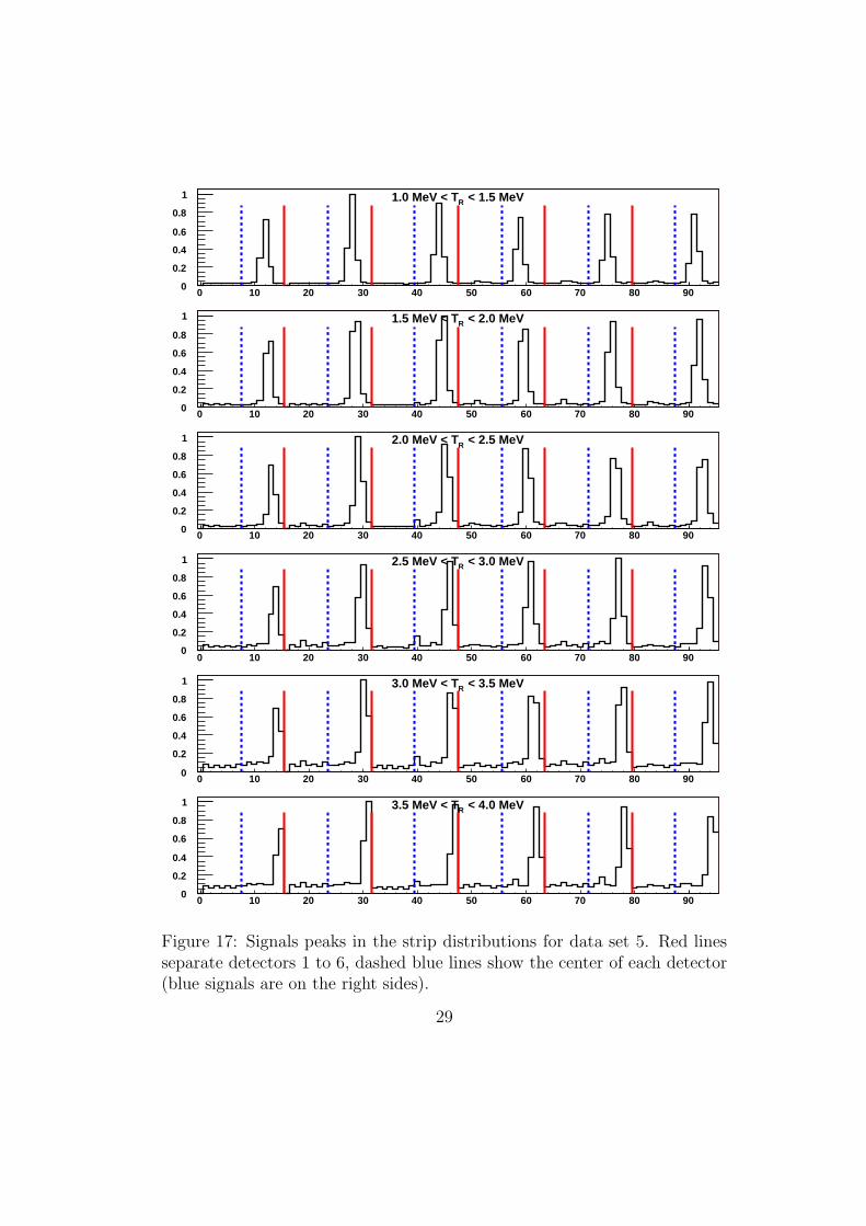
For elastically scattered protons, the scattering angle is correlated to therecoil energy. Instead of integrating over the entire detectors and all energies,the signal region can be determined as function of energy. Using 0.5 MeVwide energy bins, the peaks of the signals fall within two to three strips,compare figures 7, 13, and 14. Figures 16 and 17 show the elastic protonsignals as functions of the Silicon strip number for six different energy bins.The spectra are normalized to the highest yield in a single strip for a givenenergy bin. The red lines separate the six detectors, the dashed blue linesshow the center of each detector separating the yellow (left) and blue (right)signal sides. Energies below 1 MeV are discarded because of an increasedbackground contribution from prompt events. Above 4 MeV, most of thesignal is lost from the detector acceptance. The kinematic correlation canbe traced along the peak positions moving from the center of the detector tothe sides with increasing energy.

Instead of integrating over the whole detector and all energies, the yieldsare determined only around the peak positions for each selected energy range.This way, the background is reduced by a factor of two to four, dependingon the number of strips used for the signal region. (The final asymmetriesare calculated with two strips for the signals. For background studies, thenumber of strip is varied from one to all eight strips.)

17

3.4.1 Empty target measurements

Empty target measurements have been carried out several times during the2005 RHIC run by closing the valves of the jet target. This way, the beamgascontribution to the background can be estimated. The yields from theseruns are then scaled with the beam intensities integrated over the durationof the measurements. For measurements with one displaced beam, only theintensity of the centered beam should be used for scaling. Usually, differencesbetween relative beam intensities are small, and there is less than a 5%deviation between the results, when the scaling uses both beam intensities.Typically, the beamgas background amounts to about one fourth to one thirdof the total estimated background.

3.4.2 Abort gaps

For all but the first measurement, one of the two RHIC beams is threadedaround the jet target. The effectiveness of the displacement can be tested,by looking at yields for the signal and non-signal sides of the detectors asfunctions of bunch numbers. Each of the RHIC beams has abort gaps frombunch 112 to 119 which do not contain filled buckets. For the beam thathits the target, the abort gap shows drastically reduced yields, see the upperpart of figures 18 and 19. The blue and green curves show the yields for theblue and yellow signal sides (ns) including all proton identification cuts, thereduced yield is from the respective non-signal side (nb). Both figures areexamples from the 120-bunch mode, in which the fills did not always havethe same number of filled bunches (rising from 60 in the early fills to 111 inthe last fills). Summation over all fills then leads to the spiky structure inthe bunch distributions.

At IP12 bunch 0 of the blue beam collides with bunch 40 of the yellowbeam, indicated by the blue lines in the lower part of the figures. The abortgap of the displaced beam cannot be seen as clearly in the yield distributions.However, if one calculates the ratio of the difference of yields between signaland non-signal sides, divided by the sum, this abort gap becomes visible,too. While the figures only show examples for two measurements for recoilenergies 1.5 MeV < TR < 2.0 MeV, this difference is energy dependent andvaries between 1% and 3% in most cases.

Notice also, that the signal side yield in the respective abort gap of thecentered beam is still larger (by 20%) than the non-signal side yield. From

18

this, one can conclude that background from the displaced beam is mainlyinelastic and spreads out over the whole detectors. The same is then alsotrue for the inelastic events from the centered beam. Therefore, most ofthe bunches contain a small amount of contamination from the displacedbeam, except those from its abort gap. The step in the difference (ns −nb)/(ns+nb) is a measure of this effect. Table 3 summarizes this contributionand is later used to estimate the systematic error to describe the resultsfrom the bunch shuffling method. Comparison with table 2 shows that thistype of beam related background amounts to about one third of the totalbackground. Also, there might be overlap with the previously discussedbeamgas background.

3.5 Final Data Sets

Tables 4 and 5 present the observed number of events within a 2-strip elasticsignal region, for the left (silicon 1,2,3) and right (silicon 4,5,6) counters, foreach data set (refer to Table 1 for the data sets). We present the results in 8columns labeled NT↑

left and NT↑

right for scattering to beam left, with the target

polarized up; NT↓

left and NT↓

right for scattering to beam left and right with thetarget polarized down; and four columns for the combinations of left andright scattering with the beam polarized up and down.

19

(MeV)RT

1 2 3 4 5 6

(n

s)T

DC

t

0

20

40

60

80

100

120

(ns)TDC

t0 10 20 30 40 50 60 70 80 90

(n

s)T

oF

- t

To

Ft

-50

-40

-30

-20

-10

0

10

20

30

40

50

6.0 ( 3.7)

-50 -40 -30 -20 -10 0 10 20 30 40 50

(n

s)T

oF

- t

To

Ft

0

5000

10000

15000

20000

25000

30000

35000

40000

45000

(ns)TDC

t0 10 20 30 40 50 60 70 80 90

0

5000

10000

15000

20000

25000

30000

35000

-50 -40 -30 -20 -10 0 10 20 30 40 50

(n

s)T

oF

- t

To

Ft

0

5000

10000

15000

20000

25000

30000

35000

40000

Figure 8: Example of the time-of-flight spectrum and time offset determina-tion for a single silicon strip from the yellow 120-bunch mode measurement.The top left spectrum (t.o.f. versus recoil energy) is transformed into the topmiddle spectrum of calculated time-of-flight minus measured TDC countedtime. The contents of the blue box are projected onto the ordinate for a firstfit of the time offset. A projection onto the abscissa is used to further con-strain signal in the blue box within the red boundaries. A second projectionof the limited box is fitted for the time offset.

20

(MeV)RT

1 2 3 4 5 6

(n

s)T

DC

t

0

20

40

60

80

100

120

(ns)TDC

t0 10 20 30 40 50 60 70 80 90

(n

s)T

oF

- t

To

Ft

-50

-40

-30

-20

-10

0

10

20

30

40

50

2.0 ( 3.6)

-50 -40 -30 -20 -10 0 10 20 30 40 50

(n

s)T

oF

- t

To

Ft

0

2000

4000

6000

8000

10000

(ns)TDC

t0 10 20 30 40 50 60 70 80 90

0

1000

2000

3000

4000

5000

-50 -40 -30 -20 -10 0 10 20 30 40 50

(n

s)T

oF

- t

To

Ft

0

2000

4000

6000

8000

10000

Figure 9: Similar to figure 8, proton peaks in the non-signal region of thedetector pads have to be determined. The offsets cannot be taken from othermeasurements, because the clock synchronization changes with the beamthat is centered on the jet target.

21

channel

0 10 20 30 40 50 60 70 80 90

(n

s)0

T

-5

0

5

10

15

20

Figure 10: Time-of-flight offset determination for data set 0 (see table 1,both RHIC beams hitting the jet target). Green symbols show the results ofthe first set of fits, red are the improved fits with additional data filtering.

recoil energy d-set 2 d-set 3 d-set 4 d-set 5

1.0 MeV < TR < 1.5 Mev 4.4 % 4.0 % 2.6 % 2.8 %1.5 MeV < TR < 2.0 Mev 4.9 % 4.1 % 3.4 % 3.3 %2.0 MeV < TR < 2.5 Mev 6.7 % 5.0 % 3.5 % 3.5 %2.5 MeV < TR < 3.0 Mev 7.3 % 6.4 % 3.8 % 4.7 %3.0 MeV < TR < 3.5 Mev 8.9 % 7.4 % 5.0 % 6.6 %3.5 MeV < TR < 4.0 Mev 11.3 % 8.8 % 5.7 % 7.5 %

Table 2: Energy dependent background estimated from the non-signal sideof the detectors. Energies below 1 MeV and above 4 MeV are not furtherconsidered in the analysis because of increased background and limited ac-ceptance.

22

channel

0 10 20 30 40 50 60 70 80 90

(n

s)0

T

-8

-6

-4

-2

0

2

4

6

8

10

Figure 11: Time-of-flight offsets of the yellow beam measurement in 120-bunch mode. The offsets are comparable to those in figure 10. In both casesthe internal clock was synchronized to the yellow RHIC clock.

recoil energy d-set 2 d-set 3 d-set 4 d-set 5

1.0 MeV < TR < 1.5 Mev 1.3 % 1.3 % 1.2 % 1.1 %1.5 MeV < TR < 2.0 Mev 2.3 % 1.9 % 2.0 % 1.5 %2.0 MeV < TR < 2.5 Mev 1.4 % 2.1 % 2.1 % 1.9 %2.5 MeV < TR < 3.0 Mev 2.4 % 2.7 % 2.0 % 2.5 %3.0 MeV < TR < 3.5 Mev 3.6 % 3.8 % 2.7 % 2.8 %3.5 MeV < TR < 4.0 Mev 4.7 % 5.2 % 1.7 % 3.1 %

Table 3: Background contribution from the displaced beam estimated fromthe bunch distributions, compare figures 18 and 19. The uncertainties aredominated by the number of events in the abort gaps of the displaced beam,giving uncertainties typically less than 0.4%. For data sets 3 and 5, they are0.2% or smaller.

23

channel

0 10 20 30 40 50 60 70 80 90

(n

s)0

T

-20

-15

-10

-5

0

5

Figure 12: Time-of-flight offsets of the blue beam measurement in 120-bunchmode. The offsets are systematically about 12 ns smaller than those in figure11 where the internal clock was synchronized to the yellow instead of the blueRHIC clock.

24

T_R (MeV)

1 2 3 4 5 6 (

ns)

tof

T0

10

20

30

40

50

60

70

80

90

1

T_R (MeV)

1 2 3 4 5 6

(n

s)to

fT

0

10

20

30

40

50

60

70

80

90

0

500

1000

1500

2000

2500

3000

3500

2

T_R (MeV)

1 2 3 4 5 6

(n

s)to

fT

0

10

20

30

40

50

60

70

80

90

3

T_R (MeV)

1 2 3 4 5 6

(n

s)to

fT

0

10

20

30

40

50

60

70

80

90

0

500

1000

1500

2000

2500

3000

3500

4000

4

T_R (MeV)

1 2 3 4 5 6

(n

s)to

fT

0

10

20

30

40

50

60

70

80

90

5

T_R (MeV)

1 2 3 4 5 6

(n

s)to

fT

0

10

20

30

40

50

60

70

80

90

0

500

1000

1500

2000

2500

3000

3500

4000

4500

6

T_R (MeV)

1 2 3 4 5 6

(n

s)to

fT

0

10

20

30

40

50

60

70

80

90

7

T_R (MeV)

1 2 3 4 5 6

(n

s)to

fT

0

10

20

30

40

50

60

70

80

90

0

50

100

150

200

250

300

3508

T_R (MeV)

1 2 3 4 5 6

(n

s)to

fT

0

10

20

30

40

50

60

70

80

90

9

T_R (MeV)

1 2 3 4 5 6

(n

s)to

fT

0

10

20

30

40

50

60

70

80

90

0

50

100

150

200

250

300

350

400

10

T_R (MeV)

1 2 3 4 5 6

(n

s)to

fT

0

10

20

30

40

50

60

70

80

90

11

T_R (MeV)

1 2 3 4 5 6

(n

s)to

fT

0

10

20

30

40

50

60

70

80

90

0

50

100

150

200

250

300

350

400

12

T_R (MeV)

1 2 3 4 5 6

(n

s)to

fT

0

10

20

30

40

50

60

70

80

90

13

T_R (MeV)

1 2 3 4 5 6

(n

s)to

fT

0

10

20

30

40

50

60

70

80

90

0

50

100

150

200

250

300

350

14

T_R (MeV)

1 2 3 4 5 6

(n

s)to

fT

0

10

20

30

40

50

60

70

80

90

15

T_R (MeV)

1 2 3 4 5 6

(n

s)to

fT

0

10

20

30

40

50

60

70

80

90

0

50

100

150

200

250

300

350

16

T_R (MeV)

1 2 3 4 5 6

(n

s)to

fT

0

10

20

30

40

50

60

70

80

90

1

T_R (MeV)

1 2 3 4 5 6

(n

s)to

fT

0

10

20

30

40

50

60

70

80

90

0

500

1000

1500

2000

2500

3000

35002

T_R (MeV)

1 2 3 4 5 6

(n

s)to

fT

0

10

20

30

40

50

60

70

80

90

3

T_R (MeV)

1 2 3 4 5 6

(n

s)to

fT

0

10

20

30

40

50

60

70

80

90

0

1000

2000

3000

4000

5000

4

T_R (MeV)

1 2 3 4 5 6

(n

s)to

fT

0

10

20

30

40

50

60

70

80

90

5

T_R (MeV)

1 2 3 4 5 6

(n

s)to

fT

0

10

20

30

40

50

60

70

80

90

0

500

1000

1500

2000

2500

3000

3500

4000

6

T_R (MeV)

1 2 3 4 5 6

(n

s)to

fT

0

10

20

30

40

50

60

70

80

90

7

T_R (MeV)

1 2 3 4 5 6

(n

s)to

fT

0

10

20

30

40

50

60

70

80

90

0

50

100

150

200

250

300

3508

T_R (MeV)

1 2 3 4 5 6

(n

s)to

fT

0

10

20

30

40

50

60

70

80

90

9

T_R (MeV)

1 2 3 4 5 6

(n

s)to

fT

0

10

20

30

40

50

60

70

80

90

0

50

100

150

200

250

300

35010

T_R (MeV)

1 2 3 4 5 6

(n

s)to

fT

0

10

20

30

40

50

60

70

80

90

11

T_R (MeV)

1 2 3 4 5 6

(n

s)to

fT

0

10

20

30

40

50

60

70

80

90

0

50

100

150

200

250

300

350

12

T_R (MeV)

1 2 3 4 5 6 (

ns)

tof

T0

10

20

30

40

50

60

70

80

90

13

T_R (MeV)

1 2 3 4 5 6

(n

s)to

fT

0

10

20

30

40

50

60

70

80

90

0

50

100

150

200

250

300

350

400

14

T_R (MeV)

1 2 3 4 5 6

(n

s)to

fT

0

10

20

30

40

50

60

70

80

90

15

T_R (MeV)

1 2 3 4 5 6

(n

s)to

fT

0

10

20

30

40

50

60

70

80

90

0

50

100

150

200

250

300

350

400

450

16

Figure 13: Yields for data sample 3 in strips of detectors 3 and 6. For the yellow beam, the first and thirdlines are the signal region, lines two and four are the non-signal side.

25

T_R (MeV)

1 2 3 4 5 6 (

ns)

tof

T0

10

20

30

40

50

60

70

80

90

1

T_R (MeV)

1 2 3 4 5 6

(n

s)to

fT

0

10

20

30

40

50

60

70

80

90

0

20

40

60

80

100

120

140

160

180

200

2

T_R (MeV)

1 2 3 4 5 6

(n

s)to

fT

0

10

20

30

40

50

60

70

80

90

3

T_R (MeV)

1 2 3 4 5 6

(n

s)to

fT

0

10

20

30

40

50

60

70

80

90

0

20

40

60

80

100

120

140

160

180

200

220

4

T_R (MeV)

1 2 3 4 5 6

(n

s)to

fT

0

10

20

30

40

50

60

70

80

90

5

T_R (MeV)

1 2 3 4 5 6

(n

s)to

fT

0

10

20

30

40

50

60

70

80

90

0

20

40

60

80

100

120

140

160

180

200

220

6

T_R (MeV)

1 2 3 4 5 6

(n

s)to

fT

0

10

20

30

40

50

60

70

80

90

7

T_R (MeV)

1 2 3 4 5 6

(n

s)to

fT

0

10

20

30

40

50

60

70

80

90

0

20

40

60

80

100

120

140

160

180

200

220

240

8

T_R (MeV)

1 2 3 4 5 6

(n

s)to

fT

0

10

20

30

40

50

60

70

80

90

9

T_R (MeV)

1 2 3 4 5 6

(n

s)to

fT

0

10

20

30

40

50

60

70

80

90

0

50

100

150

200

250

10

T_R (MeV)

1 2 3 4 5 6

(n

s)to

fT

0

10

20

30

40

50

60

70

80

90

11

T_R (MeV)

1 2 3 4 5 6

(n

s)to

fT

0

10

20

30

40

50

60

70

80

90

0

500

1000

1500

2000

2500

3000

3500

12

T_R (MeV)

1 2 3 4 5 6

(n

s)to

fT

0

10

20

30

40

50

60

70

80

90

13

T_R (MeV)

1 2 3 4 5 6

(n

s)to

fT

0

10

20

30

40

50

60

70

80

90

0

500

1000

1500

2000

2500

3000

3500

14

T_R (MeV)

1 2 3 4 5 6

(n

s)to

fT

0

10

20

30

40

50

60

70

80

90

15

T_R (MeV)

1 2 3 4 5 6

(n

s)to

fT

0

10

20

30

40

50

60

70

80

90

0

500

1000

1500

2000

250016

T_R (MeV)

1 2 3 4 5 6

(n

s)to

fT

0

10

20

30

40

50

60

70

80

90

1

T_R (MeV)

1 2 3 4 5 6

(n

s)to

fT

0

10

20

30

40

50

60

70

80

90

0

20

40

60

80

100

120

140

160

180

200

220

2

T_R (MeV)

1 2 3 4 5 6

(n

s)to

fT

0

10

20

30

40

50

60

70

80

90

3

T_R (MeV)

1 2 3 4 5 6

(n

s)to

fT

0

10

20

30

40

50

60

70

80

90

0

50

100

150

200

250

4

T_R (MeV)

1 2 3 4 5 6

(n

s)to

fT

0

10

20

30

40

50

60

70

80

90

5

T_R (MeV)

1 2 3 4 5 6

(n

s)to

fT

0

10

20

30

40

50

60

70

80

90

0

20

40

60

80

100

120

140

160

180

200

220

240

6

T_R (MeV)

1 2 3 4 5 6

(n

s)to

fT

0

10

20

30

40

50

60

70

80

90

7

T_R (MeV)

1 2 3 4 5 6

(n

s)to

fT

0

10

20

30

40

50

60

70

80

90

0

50

100

150

200

250

8

T_R (MeV)

1 2 3 4 5 6

(n

s)to

fT

0

10

20

30

40

50

60

70

80

90

9

T_R (MeV)

1 2 3 4 5 6

(n

s)to

fT

0

10

20

30

40

50

60

70

80

90

0

200

400

600

800

1000

1200

1400

1600

1800

10

T_R (MeV)

1 2 3 4 5 6

(n

s)to

fT

0

10

20

30

40

50

60

70

80

90

11

T_R (MeV)

1 2 3 4 5 6

(n

s)to

fT

0

10

20

30

40

50

60

70

80

90

0

500

1000

1500

2000

250012

T_R (MeV)

1 2 3 4 5 6 (

ns)

tof

T0

10

20

30

40

50

60

70

80

90

13

T_R (MeV)

1 2 3 4 5 6

(n

s)to

fT

0

10

20

30

40

50

60

70

80

90

0

500

1000

1500

2000

2500

300014

T_R (MeV)

1 2 3 4 5 6

(n

s)to

fT

0

10

20

30

40

50

60

70

80

90

15

T_R (MeV)

1 2 3 4 5 6

(n

s)to

fT

0

10

20

30

40

50

60

70

80

90

0

500

1000

1500

2000

250016

Figure 14: Yields for data sample 5 in strips of detectors 3 and 6. For the blue beam, the second and fourthlines are the signal region, lines one and three are the non-signal side.

26

ADC peak0 20 40 60 80 100 120 140 160 180 200 220 240

AD

C in

teg

ral

0

50

100

150

200

250

1

10

210

310

410

s:adc

Figure 15: A typical distribution of ADC integral versus ADC peak counts.The lower branch is excluded from the analysis.

27

0 10 20 30 40 50 60 70 80 900

0.2

0.4

0.6

0.8

1 < 1.5 MeVR1.0 MeV < T

0 10 20 30 40 50 60 70 80 900

0.2

0.4

0.6

0.8

1 < 2.0 MeVR1.5 MeV < T

0 10 20 30 40 50 60 70 80 900

0.2

0.4

0.6

0.8

1 < 2.5 MeVR2.0 MeV < T

0 10 20 30 40 50 60 70 80 900

0.2

0.4

0.6

0.8

1 < 3.0 MeVR2.5 MeV < T

0 10 20 30 40 50 60 70 80 900

0.2

0.4

0.6

0.8

1 < 3.5 MeVR3.0 MeV < T

0 10 20 30 40 50 60 70 80 900

0.2

0.4

0.6

0.8

1 < 4.0 MeVR3.5 MeV < T

Figure 16: Signals peaks in the strip distributions for data set 3. Red linesseparate detectors 1 to 6, dashed blue lines show the center of each detector(yellow signals are on the left sides).

28

0 10 20 30 40 50 60 70 80 900

0.2

0.4

0.6

0.8

1 < 1.5 MeVR1.0 MeV < T

0 10 20 30 40 50 60 70 80 900

0.2

0.4

0.6

0.8

1 < 2.0 MeVR1.5 MeV < T

0 10 20 30 40 50 60 70 80 900

0.2

0.4

0.6

0.8

1 < 2.5 MeVR2.0 MeV < T

0 10 20 30 40 50 60 70 80 900

0.2

0.4

0.6

0.8

1 < 3.0 MeVR2.5 MeV < T

0 10 20 30 40 50 60 70 80 900

0.2

0.4

0.6

0.8

1 < 3.5 MeVR3.0 MeV < T

0 10 20 30 40 50 60 70 80 900

0.2

0.4

0.6

0.8

1 < 4.0 MeVR3.5 MeV < T

Figure 17: Signals peaks in the strip distributions for data set 5. Red linesseparate detectors 1 to 6, dashed blue lines show the center of each detector(blue signals are on the right sides).

29

bunch number0 20 40 60 80 100

b, n

sn

0

2000

4000

6000

8000

10000

12000

bunch number0 20 40 60 80 100

) b +

ns

) / (

nb

- n

s(n

0.84

0.86

0.88

0.9

0.92

0.94

0.96

0.98

Figure 18: Yield per bunch integrated over the signal sides (green) and non-signal sides (blue) of all detectors including all proton identification cuts(data set 3, yellow 120-bunch mode). The bottom plot shows the relativedifference between signal and non-signal side yields.

30

bunch number0 20 40 60 80 100

b, n

sn

0

1000

2000

3000

4000

5000

6000

7000

8000

bunch number0 20 40 60 80 100

) b +

ns

) / (

nb

- n

s(n

0.84

0.86

0.88

0.9

0.92

0.94

0.96

0.98

Figure 19: Yield per bunch integrated over the signal sides (blue) and non-signal sides (green) of all detectors including all proton identification cuts(data set 5, blue 120-bunch mode). The bottom plot shows the relativedifference between signal and non-signal side yields.

31

yellow beam TR (MeV) NT↑

left NT↑

right NT↓

left NT↓

right NB↑

left NB↑

right NB↓

left NB↓

right

0.80 48255 44850 44538 47309 48007 45985 44786 461741.25 44345 42038 40497 43986 43965 42836 40877 431881.75 35987 32869 32707 34733 35538 33574 33156 34028

data 2.25 34062 30920 30885 32561 33641 31806 31306 31675set 0 2.75 30302 28467 27663 29888 30058 29275 27907 29080

3.25 31385 24174 29015 25538 31259 25029 29141 246833.75 29542 16547 27440 16883 29623 16762 27359 166685.00 86272 24349 80234 24017 85663 24428 80843 23938

0.80 39303 42799 35319 44827 38307 43648 36315 439781.25 40364 39386 36403 42063 39735 40638 37032 408111.75 33869 32290 30386 34223 33175 32991 31080 33522

data 2.25 35372 32917 31765 34532 34582 33459 32555 33990set 2 2.75 34586 28728 31370 30438 33841 29517 32115 29649

3.25 31906 27074 28631 28315 31211 27619 29326 277703.75 32860 20116 29791 20994 32209 20482 30442 206285.00 85587 28088 78755 28028 84156 28234 80186 27882

0.80 128121 108388 125723 124416 130930 116070 122914 1167341.25 202219 193750 192697 216643 204581 204137 190335 2062561.75 179947 144277 170334 160494 181203 151385 169078 153386

data 2.25 157277 136175 148843 152041 157889 143376 148231 144840set 3 2.75 151112 135896 144384 150528 152537 142514 142959 143910

3.25 159194 116862 151969 128748 160280 122799 150883 1228113.75 135019 125290 130406 138369 136777 131264 128648 1323955.00 258003 263685 249994 286485 259996 274889 248001 275281

Table 4: Final numbers of events in the elastic signal region of two strips, for the three data sets with theyellow beam.

32

blue beam TR (MeV) NT↑

left NT↑

right NT↓

left NT↓

right NB↑

left NB↑

right NB↓

left NB↓

right

0.80 49075 49179 50930 45133 48501 47539 51504 467731.25 49029 47877 52307 43199 48756 45847 52580 452291.75 40073 39228 42263 35636 39811 37587 42525 37277

data 2.25 33686 38240 35560 34009 33773 36499 35473 35750set 0 2.75 34633 36462 36521 32949 34395 34745 36759 34666

3.25 28355 33615 29951 30535 28213 32240 30093 319103.75 20030 33400 20410 30085 19670 31964 20770 315215.00 23121 121832 23030 112545 22856 117569 23295 116808

0.80 30482 21791 32740 21078 30538 21579 32684 212901.25 26162 26550 28231 25227 26451 26093 27942 256841.75 23600 24219 26284 22912 24048 23861 25836 23270

data 2.25 20936 23823 23254 22377 21460 23224 22730 22976set 4 2.75 19097 22547 21031 21287 19371 22178 20757 21656

3.25 18773 21927 20705 20729 19030 21485 20448 211713.75 18146 20043 19747 18863 18429 19546 19464 193605.00 27559 53256 29755 51516 28035 52692 29279 52080

0.80 141378 127711 145512 114737 141232 123925 145658 1185231.25 143246 143481 148202 127498 142896 138203 148552 1327761.75 130871 133364 136042 117778 131142 128674 135771 122468

data 2.25 115010 130485 118872 115436 115107 125571 118775 120350set 5 2.75 106633 122874 109832 109266 105940 118609 110525 113531

3.25 106047 124684 108633 111680 105365 121169 109315 1151953.75 101961 114084 104840 102248 101634 110202 105167 1061305.00 157828 310933 160029 283065 156972 302513 160885 291485

Table 5: Final numbers of events in the elastic signal region of two strips, for the three data sets with theblue beam.

33

4 Asymmetries

4.1 Square-root Asymmetries

All final asymmetries have been calculated with the square-root formula [5].This analysis method uses a geometrical mean to obtain an estimate of thenumber of counts, comparing data from polarization up and down directions(target or beam) and left and right scattering. This approach can also beused to determine the acceptance or luminosity asymmetries. Below, ǫ refersto the physics asymmetry, which in the case of the polarized proton beamscattering elastically from the polarized proton target can be calculated fora polarized beam, summing over the spin states of the target to obtain anunpolarized target, and can be calculated for a polarized target, summingover the spin states of the polarized beam to obtain an unpolarized beam. 3

ǫacceptance is the acceptance asymmetry, and ǫrel−lumi is the asymmetry of theluminosities for up and down polarized target or beam:

ǫ =

√

N↑

left · N↓

right −√

N↓

left · N↑

right√

N↑

left · N↓

right +√

N↓

left · N↑

right

(5)

ǫacceptance =

√

N↑

left · N↓

left −√

N↑

right · N↓

right√

N↑

left · N↓

left +√

N↑

right · N↓

right

(6)

ǫrel.lumi =

√

N↑

left · N↑

right −√

N↓

left · N↓

right√

N↑

left · N↑

right +√

N↓

left · N↓

right

(7)

Figures 20 and 21 shows results for data sets 3 and 5 of the square rootasymmetries at recoil energies 1.5 MeV < TR < 2.0 MeV. The vertical dashedlines separate the three detector pairs. Both the physical and the luminosityasymmetries are emerging in the strips of the signal region. Although thestastical accuracy is lacking, we see no indication of an asymmetry in thebackground strips.

3Residual polarization, for example for residual target polarization in the beamasymmetry ǫbeam, contributes at third order, with a correction factor of ǫbeam × (1 +

(ANPT ǫTargetrel.lumi)

2). For the observed values of ǫTargetrel.lumi=0.02, this correction is about

10−6 × ǫbeam.

34

strip0 5 10 15 20 25 30 35 40 45

∈ta

rget

-0.06

-0.04

-0.02

-0

0.02

0.04

strip0 5 10 15 20 25 30 35 40 45

rel.l

um

i.∈

-0.02

0

0.02

0.04

0.06

strip0 5 10 15 20 25 30 35 40 45

∈b

lue

-0.05

-0.04

-0.03

-0.02

-0.01

0

0.01

0.02

0.03

0.04

strip0 5 10 15 20 25 30 35 40 45

rel.l

um

i.∈

-0.02

-0.01

0

0.01

0.02

0.03

0.04

strip0 5 10 15 20 25 30 35 40 45

∈ye

llow

-0.03

-0.02

-0.01

0

0.01

0.02

0.03

0.04

strip0 5 10 15 20 25 30 35 40 45

rel.l

um

i.∈

-0.02

-0.01

0

0.01

0.02

0.03

0.04

0.05

0.06

Figure 20: Square root asymmetries for data set 3 at recoil energies 1.5 MeV< TR < 2.0 MeV.

35

strip0 5 10 15 20 25 30 35 40 45

∈ta

rget

-0.06

-0.04

-0.02

-0

0.02

0.04

strip0 5 10 15 20 25 30 35 40 45

rel.l

um

i.∈

-0.02

0

0.02

0.04

0.06

strip0 5 10 15 20 25 30 35 40 45

∈b

lue

-0.06

-0.04

-0.02

-0

0.02

0.04

strip0 5 10 15 20 25 30 35 40 45

rel.l

um

i.∈

-0.04

-0.02

0

0.02

0.04

0.06

strip0 5 10 15 20 25 30 35 40 45

∈ye

llow

-0.06

-0.04

-0.02

-0

0.02

0.04

strip0 5 10 15 20 25 30 35 40 45

rel.l

um

i.∈

-0.04

-0.02

0

0.02

0.04

Figure 21: Square root asymmetries for data set 5 at recoil energies 1.5 MeV< TR < 2.0 MeV.

36

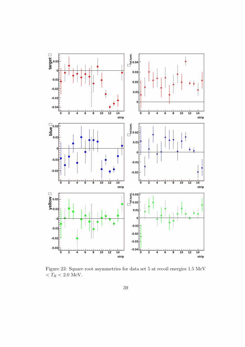
Figures 22 and 23 use the combined yields of all left and right side de-tectors, that have been kept separated in figures 20 and 21. The verticaldashed lines here divide the signal side on the detectors from the non-signalsides. Again, no indication of any background asymmetry can be seen withinthe statistical errors. The luminosity asymmetries are also shown; they arethe same for the three elastic signal regions for the three detector pairs, andshow some variation for the background regions.

After extensive cross checks with simple and square-root asymmetries,we go on to calculate the asymmetries as functions of recoil energy TR onlywithin the determined signal strips. These asymmetry calculations use themeasured number of elastic events given in tables 4 and 5. The results arepresented for each data set in tables 6 and 7. Note that the uncertainties forthe asymmetries are ∆ǫ=1/

√Ntotal, where Ntotal is the total number of events,

and the uncertainty is the same for the beam and target asymmetries. Thetable also presents the asymmetry ratio r = ǫbeam/ǫtarget, and its uncertainty.

This uncertainty is δr/r = (1/AN)×√

1/P 2

beam + 1/P 2target×

√

1/Ntotal. with

Pbeam = r×Ptarget and Ptarget independently measured. AN is obtained fromthe target asymmetry and target polarization, AN = ǫtarget/Ptarget.

Figures 24 to 27 present the asymmetry results and asymmetry ratiosfor data sets 2 through 5. The measured asymmetries are compared to anexisting formal description of the analyzing power AN in terms of helicityamplitudes φ1 to φ5 [1], which is scaled with the jet target polarization (solidred line) and the determined beam polarization (dashed green or blue line).These curves are not fitted to the data and are only meant to guide the eye.

Energies below TR = 1 MeV and above TR = 4 MeV are not consid-ered further for the beam polarization determination because of asymmetricacceptance and increased background (note the drop-off in all asymmetriesabove 4 MeV).

The beam polarization Pbeam is derived from the target (ǫtarget) and thebeam (ǫbeam) related asymmetries and the independently measured targetpolarization Ptarget:

Pbeam

Ptarget

=ǫbeam

ǫtarget

. (8)

The errors for the asymmetry ratios, presented above with the table, arecalculated from the independent measurements of the numbers of elasticevents given in tables 4 and 5, and are identical to the result of treatingthe measurements of ǫbeam and ǫtarget as independent measurements. We

37

strip0 2 4 6 8 10 12 14

∈ta

rget

-0.02

-0.01

0

0.01

0.02

0.03

0.04

strip0 2 4 6 8 10 12 14

rel.l

um

i.∈

-0.02

-0.01

0

0.01

0.02

0.03

0.04

0.05

strip0 2 4 6 8 10 12 14

∈b

lue

-0.015

-0.01

-0.005

0

0.005

0.01

0.015

0.02

strip0 2 4 6 8 10 12 14

rel.l

um

i.∈

0

0.005

0.01

0.015

0.02

0.025

0.03

strip0 2 4 6 8 10 12 14

∈ye

llow

-0.015

-0.01

-0.005

-0

0.005

0.01

0.015

0.02

0.025

strip0 2 4 6 8 10 12 14

rel.l

um

i.∈

-0.005

0

0.005

0.01

0.015

0.02

0.025

0.03

0.035

Figure 22: Square root asymmetries for data set 3 at recoil energies 1.5 MeV< TR < 2.0 MeV.

38

strip0 2 4 6 8 10 12 14

∈ta

rget

-0.04

-0.03

-0.02

-0.01

0

0.01

strip0 2 4 6 8 10 12 14

rel.l

um

i.∈

0

0.01

0.02

0.03

0.04

strip0 2 4 6 8 10 12 14

∈b

lue

-0.02

-0.01

0

0.01

0.02

strip0 2 4 6 8 10 12 14

rel.l

um

i.∈

-0.02

-0.01

0

0.01

0.02

strip0 2 4 6 8 10 12 14

∈ye

llow

-0.03

-0.02

-0.01

-0

0.01

0.02

strip0 2 4 6 8 10 12 14

rel.l

um

i.∈

-0.04

-0.03

-0.02

-0.01

0

0.01

0.02

0.03

Figure 23: Square root asymmetries for data set 5 at recoil energies 1.5 MeV< TR < 2.0 MeV.

39

yellow beam TR ǫtarget ǫbeam ∆ǫ r = ǫbeam

ǫtarget∆r

(MeV) (%) (%) (%) (%) (%)

1.25 3.40 2.02 0.24 59.6 8.31.75 3.77 2.07 0.27 55.0 8.2

data 2.25 3.74 1.70 0.28 45.3 8.2set 0 2.75 3.49 1.69 0.29 48.3 9.3

3.25 3.33 1.41 0.30 42.2 9.93.75 2.35 1.85 0.34 78.7 18.7

1.0-4.0 51.8 3.8

1.25 4.22 1.87 0.25 44.2 6.51.75 4.16 2.03 0.28 48.7 7.4

data 2.25 3.88 1.90 0.27 49.0 7.8set 2 2.75 3.88 1.42 0.28 36.6 7.8

3.25 3.83 1.69 0.29 44.3 8.43.75 3.52 1.59 0.32 45.1 9.9

1.0-4.0 44.7 3.2

1.25 4.00 2.06 0.11 51.6 3.11.75 4.03 2.06 0.12 51.1 3.4

data 2.25 4.13 1.83 0.13 44.3 3.4set 3 2.75 3.69 1.86 0.13 50.5 4.0

3.25 3.58 1.51 0.13 42.2 4.13.75 3.35 1.75 0.14 52.1 4.6

1.0-4.0 48.7 1.5

Table 6: Final asymmetries in the elastic signal region of two strips, for thethree data sets with the yellow beam.

40

blue beam TR ǫtarget ǫbeam ∆ǫ r = ǫbeam

ǫtarget∆r

(MeV) (%) (%) (%) (%) (%)

1.25 4.19 2.23 0.23 53.2 6.21.75 3.73 1.86 0.25 49.8 7.6

data 2.25 4.28 1.75 0.27 40.8 6.7set 0 2.75 3.86 1.72 0.27 44.5 7.6

3.25 3.77 1.87 0.29 49.6 8.53.75 3.08 1.71 0.32 55.5 11.8

1.0-4.0 48.2 3.1

1.25 3.18 1.77 0.31 55.5 11.01.75 4.08 2.42 0.32 59.3 9.2

data 2.25 4.19 1.71 0.33 40.7 8.6set 4 2.75 3.85 2.32 0.35 60.4 10.5

3.25 3.85 2.16 0.35 56.2 10.43.75 3.63 1.60 0.36 44.2 10.9

1.0-4.0 52.2 4.1

1.25 3.80 1.97 0.13 51.9 4.01.75 4.07 2.10 0.14 51.6 3.8

data 2.25 3.89 1.85 0.14 47.5 4.1set 5 2.75 3.67 2.15 0.15 58.6 4.7

3.25 3.35 2.18 0.15 65.1 5.33.75 3.43 1.80 0.15 52.3 5.1

1.0-4.0 53.5 1.8

Table 7: Final asymmetries in the elastic signal region of two strips, for thethree data sets with the blue beam.

41

(MeV)T1 2 3 4 5 6

∈as

ymm

etry

0

0.01

0.02

0.03

0.04

0.05target asymmetrybeam asymmetry

Figure 24: Square root asymmetries for data set 2 (yellow beam, 60-bunchmode) as functions of recoil energy TR.

determine a TR-dependent asymmetry ratio mainly to reduce the containedbackground in the yields, before calculating the weighted mean. Cross checkswith integrated yields show that the functional form of AN is negligible forthe determination of the beam polarization.

4.2 Background Contributions in Asymmetry Ratios

As shown in the previous chapter (table 2), the background below the signalregion can be estimated from the non-signal sides of the detectors. Thisbackground can be as large as 10% of the signal height and in the followingleads to reduced asymmetries by the same fraction. If the background ispolarization dependent, this must also be considered in the determination ofthe analyzing power.

For the 2005 data, the primary objective is the determination of the beampolarization and not the analyzing power of elastic proton-proton scatteringitself. Therefore, combination of equation 8 with the respective asymme-try formulas removes polarization independent background from the beampolarization result. For simple asymmetries, the denominator of both asym-metries (i.e. the sum over both polarization states) is the same, while thenumerator (the difference of both polarization states) removes all polarization

42

(MeV)T1 2 3 4 5 6

∈as

ymm

etry

0

0.01

0.02

0.03

0.04

0.05target asymmetrybeam asymmetry

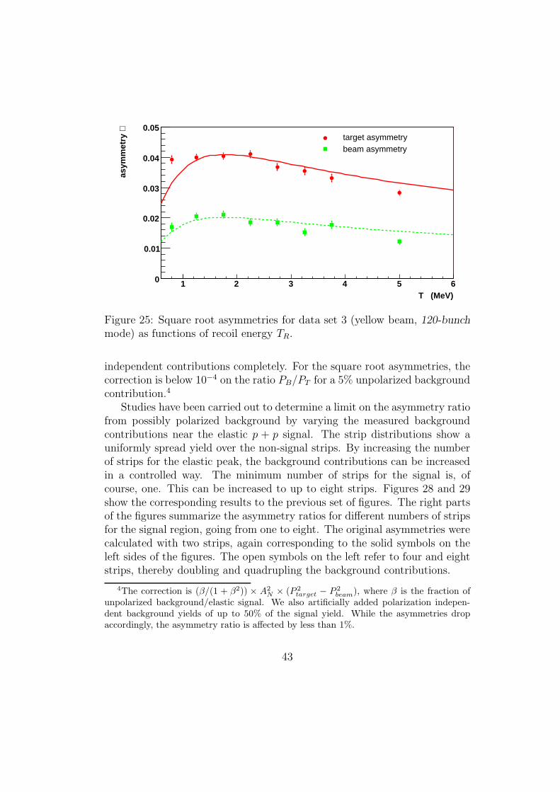
Figure 25: Square root asymmetries for data set 3 (yellow beam, 120-bunchmode) as functions of recoil energy TR.

independent contributions completely. For the square root asymmetries, thecorrection is below 10−4 on the ratio PB/PT for a 5% unpolarized backgroundcontribution.4

Studies have been carried out to determine a limit on the asymmetry ratiofrom possibly polarized background by varying the measured backgroundcontributions near the elastic p + p signal. The strip distributions show auniformly spread yield over the non-signal strips. By increasing the numberof strips for the elastic peak, the background contributions can be increasedin a controlled way. The minimum number of strips for the signal is, ofcourse, one. This can be increased to up to eight strips. Figures 28 and 29show the corresponding results to the previous set of figures. The right partsof the figures summarize the asymmetry ratios for different numbers of stripsfor the signal region, going from one to eight. The original asymmetries werecalculated with two strips, again corresponding to the solid symbols on theleft sides of the figures. The open symbols on the left refer to four and eightstrips, thereby doubling and quadrupling the background contributions.

4The correction is (β/(1 + β2)) × A2

N × (P 2

target − P 2

beam), where β is the fraction ofunpolarized background/elastic signal. We also artificially added polarization indepen-dent background yields of up to 50% of the signal yield. While the asymmetries dropaccordingly, the asymmetry ratio is affected by less than 1%.

43

(MeV)T1 2 3 4 5 6

∈as

ymm

etry

0

0.01

0.02

0.03

0.04

0.05target asymmetrybeam asymmetry

Figure 26: Square root asymmetries for data set 4 (blue beam, 60-bunchmode) as functions of recoil energy TR.

While the variations are smaller than the statistical errors, these differ-ences do not necessarily point to a polarization dependence of inelastic eventsbut might well be just statistical fluctuations.5 Also, no clear asymmetry hasbeen seen in figures 20 through 23.

The conclusion from the variations of signal strips is that the backgroundyields below the elastic peak contribute at most 1.1% to the asymmetry ratio,where we use the largest change observed. The systematic error for the beampolarization scales with the target polarization, accordingly.

4.3 Bunch Shuffling

Certain beam related systematic errors can be explored with the bunch shuf-fling technique. In this method, the polarization direction of each RHICbunch is randomly assigned and the resulting asymmetries are calculated.6

5The deteriorating statistical accuracy is less obvious, because the single strip resultscontain only about half of the elastic statistics of two strips and there can also be elasticevents in a third strip. Again, the blue asymmetry ratio seems to drop slightly, and theyellow asymmetry rises.

6While a randomized polarization pattern and randomization of single events both leadto an unpolarized beam, the first approach still assumes polarization of single bunches and

44

This process is repeated several thousand times. Systematic errors are di-luted by the statistical accuracy of the data sample, which is usually thedominant part of the uncertainties.

The bunch shuffling results are shown in figures 30 and 31 for the twodata sets with the highest statistics. Beam asymmetries were calculated asweighted means for separate recoil energies, the target asymmetries were notconsidered. Asymmetries from integrated yields over all energies have beencross checked and show similar results. Each figure contains 5000 iterationsof the randomization process and the asymmetries have been scaled withreciprocal statistical errors. The average asymmetry should be zero by con-struction. The distributions for the randomized patterns are gaussian witha width of one if the associated errors are purely stochastic. Gaussian fits tothe distributions are also included in the figures and they describe the shapewell for all asymmetries.

Emphasis has to be put to the yellow beam (green curve) in figure 30and the blue beam in figure 31, compare table 8. In both cases, the width isslightly enhanced. The number of bunches n can have an effect on the widthof the distributions, leading to larger deviations for fewer bunches that arepart of the randomization:

σshuffle =1√

n − 1. (9)

The average number of bunches for the relevant data sets is 80 to 100, leadingto σshuffle ≈ 0.12, which still does not cover the observed widths. Obviously,for these two data sets the statistical accuracy is in the range of an emergingsystematic uncertainty. The other data sets have significantly less statistics,which does not mean that they don’t suffer from the same systematic errors.It is further noticeable, that the displaced beam asymmetries do not showthe same discrepancies.

Table 8 indicates that there is some beam related systematic uncertainty.Differences between yields for different bunch numbers have been seen andhave been associated to the displaced beam, the beam threaded around thetarget, compare abort gap studies in the previous chapter. A rough estimateof the systematic error arising from these differences has been added to thestatistical errors and the total error has then been used in the bunch shuffling.As a result, the widths of the problematic beams fall off to 1.09 and 1.13 andare consistent with one. All other widths are minimally, if at all, affected.

is sensitive to differences between separate bunches.

45

data set ǫblue σ(ǫblue) ǫyellow σ(ǫyellow)

0 0.018 1.06 0.014 1.092 -0.043 1.01 -0.021 1.113 -0.005 1.11 0.005 1.324 -0.007 1.07 -0.007 1.025 0.014 1.27 -0.013 1.03

Table 8: Results from the bunch shuffling method. For data sets 3 and 5,the centered beam asymmetry distributions show an increased width (ǫyellow

for data set 3 and ǫyellow for data set 5).

data set beam r = ǫbeam/ǫtarget σr Pbeam σPbeam(stat)

0 yellow 0.5183 0.0381 47.89% 3.52%0 blue 0.4821 0.0309 44.55% 2.86%2 yellow 0.4466 0.0317 41.27% 2.93%3 yellow 0.4872 0.0151 45.02% 1.40%4 blue 0.5220 0.0406 48.23% 3.75%5 blue 0.5353 0.0179 49.46% 1.65%

Table 9: Results of the asymmetry ratios, beam polarizations, and statisticalerrors.

4.4 Beam Polarizations

The final asymmetry ratios and beam polarizations with their statisticalerrors are summarized in table 9. The beam polarizations are obtainedfrom the asymmetry ratios presented in tables 6 and 7, using the indepen-dently measured jet polarization discussed in Section 2.1. The jet polar-ization was Ptarget = (92.4 ± 1.8)%, with the uncertainty from estimatingthe unpolarized molecular contribution to the polarized atomic hydrogen jettarget. The uncertainties in the table are statistical. The global system-atic uncertainty is obtained from the quadratic sum of the molecular frac-tion uncertainty and the background uncertainty for the asymmetry ratio r:∆Pbeam/Pbeam(syst) =

√

(0.018/Ptarget)2 + (0.011/r)2. With r ≈0.5, this is

∆Pbeam/Pbeam(syst) = ±√

0.01952 + 0.0222=±0.029.Figure 32 shows a comparison of the final polarization values determined

46

with the jet polarimeter with online numbers taken with the Carbon po-larimeters (blue in the top and yellow in the bottom part of the figure). Theabscissa is in units of days, starting shortly before April 22 and running untilJune 24. The online numbers are displayed by the red circles. Underlyingthe circles are colored (blue and yellow) boxes which indicate a ± one sigmaband of the jet polarization in the respective data sub-sample. The verti-cal dashed line show a change of the jet polarimeter target setup, either achange in the 60/120-bunch mode, movement/displacement of RHIC beams,or change of RHIC energies. For reference, each of the sub-figures containsa colored band starting with green on the left side. Green regions refer tothe both-beam mode in the beginning of the run. Yellow and blue regionsare, of course, measurements with the blue (yellow, resp.) beam displaced.Dashed bands indicate the 60-bunch mode, filled bands are measurements inthe 120-bunch mode. Also, there is a short magenta region of 205 GeV/ccommissioning, where the data are not presented. Near the right edge, afew measurements in a single fill have been excluded from the jet analysisbecause both beams were slightly displaced.

47

(MeV)T1 2 3 4 5 6

∈as

ymm

etry

0

0.01

0.02

0.03

0.04

0.05target asymmetrybeam asymmetry

Figure 27: Square root asymmetries for data set 5 (blue beam, 120-bunchmode) as functions of recoil energy TR.

(MeV)RT1 2 3 4 5 6

∈as

ymm

etry

0

0.01

0.02

0.03

0.04

0.05

signal strip width1 2 3 4 5 8

asym

met

ry r

atio

0.47

0.48

0.49

0.5

0.51

0.52

Figure 28: Background contributions to asymmetries and asymmetry ratiosfor data set 3, see text for details about the symbols in the left figure.

48

(MeV)RT1 2 3 4 5 6

∈as

ymm

etry

0

0.01

0.02

0.03

0.04

0.05

signal strip width1 2 3 4 5 8

asym

met

ry r

atio

0.52

0.53

0.54

0.55

0.56

Figure 29: Background contributions to asymmetries and asymmetry ratiosfor data set 5, see text for details about the symbols in the left figure.

σ / ∈-5 -4 -3 -2 -1 0 1 2 3 4 50

50

100

150

200

250

300

350

σ / ∈-5 -4 -3 -2 -1 0 1 2 3 4 50

50

100

150

200

250

300

Figure 30: Bunch shuffling results (5000 repetitions) for data set 3. Asym-metries have been scaled with statistical errors to make deviations from theexpected shape more distinctive.

49

σ / ∈-5 -4 -3 -2 -1 0 1 2 3 4 50

50

100

150

200

250

300

350

σ / ∈-5 -4 -3 -2 -1 0 1 2 3 4 50

50

100

150

200

250

300

350

400

Figure 31: Bunch shuffling results (5000 repetitions) for data set 5.

50

04-22 04-29 05-06 05-13 05-20 05-27 06-03 06-10 06-17 06-240

10

20

30

40

50

60

70

80

04-22 04-29 05-06 05-13 05-20 05-27 06-03 06-10 06-17 06-240

10

20

30

40

50

60

70

80

Figure 32: Comparison of results of the jet polarimeter (colored boxes) withthe pC-polarimeter online numbers (red circles) (top: blue beam polariza-tions, bottom: yellow beam polarizations). The vertical dashed lines indicatea change of the jet polarimeter setup. Detailed explanation of color codes inthe text.

51

References

[1] H. Okada et al., Phys. Lett. B638, 450 (2006).

[2] A. Zelinski et al., Nucl. Instr. Meth. A536, 248 (2005); T. Wise et al.,Nucl. Instr. Meth. A559, 1 (2006).

[3] H. Okada, Doctor of Science Thesis, Kyoto University (2006).

[4] M.J. Berger et al., http://physics.nist.gov/ PhysicsRef-Data/Star/Text/contents.html

[5] G.G. Ohlsen and P.W. Keaton Techniques for measurement of spin-1

2and

spin-1 polarization analyzing tensors. Nucl. Instr. and Meth. 109 (1973),41.

[6] I. Nakagawa et al., CNIpol analysis note for 2005, CAD Note 275.

52