c 2016 varun badrinath krishna - university of illinoisvarun badrinath krishna thesis submitted in...
TRANSCRIPT

c© 2016 Varun Badrinath Krishna

AN ENERGY-EFFICIENT P2P PROTOCOL FOR VALIDATING MEASUREMENTSIN WIRELESS SENSOR NETWORKS
BY
VARUN BADRINATH KRISHNA
THESIS
Submitted in partial fulfillment of the requirementsfor the degree of Master of Science in Electrical and Computer Engineering
in the Graduate College of theUniversity of Illinois at Urbana-Champaign, 2016
Urbana, Illinois
Adviser:
Professor William H. Sanders

ABSTRACT
Wireless sensor networks (WSNs) should collect accurate measurements to reliably capture
the state of the environment that they monitor. However, measurement data collected from
one or more sensors may drift or become erroneous due to hardware failures or sensor degra-
dation. In WSNs with remote deployments, detecting those measurement errors through a
centralized reporting approach can result in a large number of message transmissions, which
in turn dramatically decreases the battery life of sensors in the network. In this thesis,
we address this issue through three main contributions. First, we propose a protocol in
which sensors detect errors in a peer-to-peer (P2P) fashion, and that extends the life of the
WSN by minimizing the number of messages transmitted. Second, we propose an effective
anomaly detection approach that has low memory and processing requirements, allowing for
easy deployment on low-cost sensor hardware. Third, we develop a trace-driven, discrete-
event simulator that allows us to evaluate the developed protocol and approach. In doing so,
we use three datasets from real WSN deployments, which include indoor air temperature,
sea surface water temperature and seismic wave amplitude sensors. Our results show that
our P2P protocol can accurately detect errors and simultaneously extend the effective WSN
lifetime dramatically compared to the centralized protocol.
ii

To Bill Sanders, Marianne Winslett and David Yau.
iii

ACKNOWLEDGMENTS
I would first like to acknowledge Michael Rausch and Benjamin Ujcich for their contributions
to this work. They contributed to the abstract, introduction and related work sections of
this thesis. They also helped with improving the quality of the writing. Most importantly,
the brainstorming sessions with them produced some of the main ideas in this thesis.
I would like to thank the following people:
• Prof. William Sanders, Dr. Kiryung Lee and Prof. Indranil Gupta for their technical
guidance on the project that led to this thesis. Several aspects of the thesis, including
writing and organization were improved based on their feedback.
• Prof. Marianne Winslett, Prof. David Yau and Dr. Bimlesh Wadhwa, who recom-
mended me for graduate school.
• Prof. Sanders, Prof. Winslett and Prof. Ravishankar Iyer for their continued support
of my endeavors.
• Jenny Applequist, James Hutchinson, Aarti Shah, Dr. Wander Wadman, Brett Fed-
dersen, and Sangeetha A. J. for their help with proof-reading and improving the writing
quality of the thesis.
• My colleagues in the PERFORM Group (Ahmed Fawaz, Atul Bohara, Ben Ujcich,
Carmen Cheh, Ken Keefe, Michael Rausch, Mohammad Noureddine, Ronald Wright,
and Uttam Thakore) for their support.
• My colleagues in the Information Trust Institute (Prof. David Nicol, Amy Irle, Tim
Yardley, Jeremy Jones, Tonia Siuts, Amy Clay, Cheri Soliday, Al Valdes) for their
support.
iv

• My former colleagues in the Advanced Digital Sciences Center (Prof. Douglas Jones,
Dr. Rui Tan, Dr. Deokwoo Jung, Dr. Binbin Chen, Nguyen Hoang Hai, William
Temple, and Ngo Quang Minh Khiem), from whom I have learned a lot.
• The authors of the papers that I have cited in this thesis. They have provided an
invaluable knowledgebase.
• My friends and family for their support.
We use three datasets in this study and thank the providers. First, the GeoNet Project
in New Zealand for the seismic waveform data [1] (and, in particular, Kevin Fenaughty for
his assistance). Second, the TAO Project Office of NOAA/PMEL for the sea water surface
temperature data. Finally, the Intel Berkeley Research Lab [2] for the indoor air temperature
data.
Finally, I would like to thank the University of Illinois at Urbana-Champaign for providing
me with a highly conducive environment for research, access to great people and resources,
travel opportunities, and social opportunities.
v

TABLE OF CONTENTS
LIST OF FIGURES . . . . . . . . . . . . . . . . . . . . . . . . . . . . . . . . . . . . viii
LIST OF ABBREVIATIONS . . . . . . . . . . . . . . . . . . . . . . . . . . . . . . . xi
CHAPTER 1 INTRODUCTION . . . . . . . . . . . . . . . . . . . . . . . . . . . . 1
CHAPTER 2 PRELIMINARIES . . . . . . . . . . . . . . . . . . . . . . . . . . . . 42.1 System Model . . . . . . . . . . . . . . . . . . . . . . . . . . . . . . . . . . . 42.2 Failure Model . . . . . . . . . . . . . . . . . . . . . . . . . . . . . . . . . . . 52.3 Protocol Requirement . . . . . . . . . . . . . . . . . . . . . . . . . . . . . . 52.4 Evaluation Metrics . . . . . . . . . . . . . . . . . . . . . . . . . . . . . . . . 6
CHAPTER 3 POTENTIAL APPLICATIONS . . . . . . . . . . . . . . . . . . . . . 83.1 Indoor Air Temperature of an Office (Berkeley) . . . . . . . . . . . . . . . . 83.2 Sea Surface Temperatures (TAO) . . . . . . . . . . . . . . . . . . . . . . . . 83.3 Seismic Wave Measurement Data (NZ) . . . . . . . . . . . . . . . . . . . . . 12
CHAPTER 4 P2P ERROR DETECTION PROTOCOL . . . . . . . . . . . . . . . 164.1 Protocol Description . . . . . . . . . . . . . . . . . . . . . . . . . . . . . . . 164.2 Required Properties of the Anomaly Detection Approach and
Similarity Metric . . . . . . . . . . . . . . . . . . . . . . . . . . . . . . . . . 204.3 Memory Requirement . . . . . . . . . . . . . . . . . . . . . . . . . . . . . . . 214.4 Handling Changes in the Network . . . . . . . . . . . . . . . . . . . . . . . . 214.5 Proof of Energy-Optimality . . . . . . . . . . . . . . . . . . . . . . . . . . . 224.6 Main Strength and Limitation . . . . . . . . . . . . . . . . . . . . . . . . . . 25
CHAPTER 5 VALIDATION OF SENSOR MEASUREMENTS . . . . . . . . . . . 275.1 Summary of Approach . . . . . . . . . . . . . . . . . . . . . . . . . . . . . . 275.2 Anomaly Detection Approach Assumptions . . . . . . . . . . . . . . . . . . . 285.3 Isocontours of the Bivariate Normal Distribution . . . . . . . . . . . . . . . . 295.4 Anomaly Detection Procedure . . . . . . . . . . . . . . . . . . . . . . . . . . 345.5 Similarity Metric . . . . . . . . . . . . . . . . . . . . . . . . . . . . . . . . . 385.6 Demonstrating Required Properties of Approach . . . . . . . . . . . . . . . . 395.7 Illustration of Approach on Datasets . . . . . . . . . . . . . . . . . . . . . . 42
vi

CHAPTER 6 PROTOCOL EVALUATION . . . . . . . . . . . . . . . . . . . . . . 486.1 Sensor Network Protocol Simulator . . . . . . . . . . . . . . . . . . . . . . . 486.2 Protocol Implementation . . . . . . . . . . . . . . . . . . . . . . . . . . . . . 516.3 Detection Accuracy Results . . . . . . . . . . . . . . . . . . . . . . . . . . . 706.4 Reachability Results . . . . . . . . . . . . . . . . . . . . . . . . . . . . . . . 70
CHAPTER 7 RELATED WORK . . . . . . . . . . . . . . . . . . . . . . . . . . . . 77
CHAPTER 8 CONCLUSION . . . . . . . . . . . . . . . . . . . . . . . . . . . . . . 80
APPENDIX A UNSUITABLE ANOMALY DETECTIONAPPROACHES . . . . . . . . . . . . . . . . . . . . . . . . . . . . . . . . . . . . . 81A.1 OLS Linear Regression . . . . . . . . . . . . . . . . . . . . . . . . . . . . . . 81A.2 TLS Linear Regression . . . . . . . . . . . . . . . . . . . . . . . . . . . . . . 83A.3 Correlation and Dot Products . . . . . . . . . . . . . . . . . . . . . . . . . . 85
APPENDIX B SENSOR ID AND NAME MAPPING . . . . . . . . . . . . . . . . . 86B.1 Berkeley Dataset . . . . . . . . . . . . . . . . . . . . . . . . . . . . . . . . . 86B.2 TAO Dataset . . . . . . . . . . . . . . . . . . . . . . . . . . . . . . . . . . . 86B.3 NZ Dataset . . . . . . . . . . . . . . . . . . . . . . . . . . . . . . . . . . . . 86
REFERENCES . . . . . . . . . . . . . . . . . . . . . . . . . . . . . . . . . . . . . . . 89
vii

LIST OF FIGURES
3.1 Sample of temperature data from Intel Berkeley Research. The white spotsare anomalous measurements. . . . . . . . . . . . . . . . . . . . . . . . . . . 9
3.2 Sample of sea surface temperature data from the Tropical AtmosphereOcean Project by the Pacific Environmental Laboratory. The white spotin Sensor 2 is an anomaly. . . . . . . . . . . . . . . . . . . . . . . . . . . . . 9
3.3 TAO Dataset: linear relationships and closeness in measurements valuesas a function of physical distance. . . . . . . . . . . . . . . . . . . . . . . . . 10
3.4 Sample of the seismic waveform data in the GeoNet National SeismographNetwork in New Zealand. Note that the seismic amplitude has no unitspecified since the data is uncalibrated. . . . . . . . . . . . . . . . . . . . . . 12
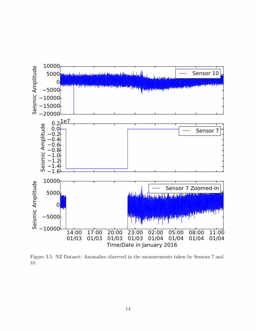
3.5 NZ Dataset: Anomalies observed in the measurements taken by Sensors 7and 10. . . . . . . . . . . . . . . . . . . . . . . . . . . . . . . . . . . . . . . . 14
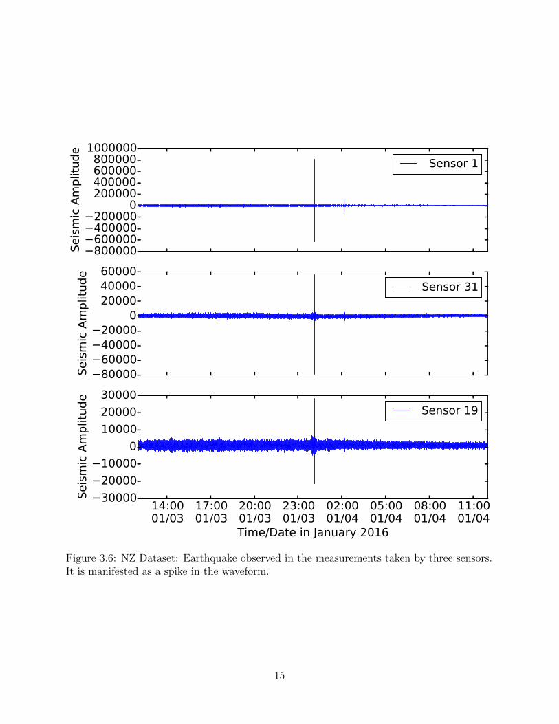
3.6 NZ Dataset: Earthquake observed in the measurements taken by threesensors. It is manifested as a spike in the waveform. . . . . . . . . . . . . . . 15
4.1 P2P protocol at each sensor . . . . . . . . . . . . . . . . . . . . . . . . . . . 174.2 P2P protocol for Stage 1 (complete stage1) at each sensor . . . . . . . . . . 184.3 P2P protocol for Stage 2 (complete stage2) at each sensor . . . . . . . . . . 194.4 P2P Protocol for Stage 3 at sink . . . . . . . . . . . . . . . . . . . . . . . . . 204.5 WSN showing the routing path of the optimal message in our protocol
that reports the erroneous measurement (solid red arrow), unnecessarymessages that report anomalous measurements (dashed red arrows), andmessages containing measurements (dotted blue arrows). Sensor S(1) is faulty. 22
5.1 Single anomalous measurement (in red) in the NZ dataset is detected byconstructing an isocontour (blue shaded elliptical region) as a detectionboundary. Normal measurements are inside the isocontour and are jointlyGaussian. . . . . . . . . . . . . . . . . . . . . . . . . . . . . . . . . . . . . . 28
5.2 Anomalies (red crosses) in the NZ dataset due to earthquake observed innormalized measurement space (left) and the space spanned by the twoprincipal components (right). . . . . . . . . . . . . . . . . . . . . . . . . . . 32
5.3 Anomalies (yellow stars) due to the earthquake presented in the seismicwaveform in the NZ Dataset (200 sec view). . . . . . . . . . . . . . . . . . . 43
viii

5.4 Anomalies (red crosses) in the three datasets are egregious. They wouldbe detected even if the isocontour were drawn 75, 500 and 3600 standarddeviations from the mean in the Berkeley, TAO and NZ datasets, respectively. 44
5.5 Map of physical location of select seismic wave sensors in the NZ dataset.The four sensors grouped in the largest circle are located around a volcano. . 46
6.1 Components of the custom-built discrete event simulator. . . . . . . . . . . . 496.2 Centralized validation protocol (Berkeley: Actual Layout): Battery life
illustration for static routing with routing paths shown for 4 arbitrarysensors. Sink is the star in the center. Crossed-out sensors are unreachable. . 57
6.3 P2P validation protocol (Berkeley: Actual Layout): Battery life illustra-tion for static routing with routing paths shown for 4 arbitrary sensors.Sink is the star in the center. Crossed-out sensors are unreachable. . . . . . . 58
6.4 Centralized validation protocol (Berkeley: Actual Layout): Battery lifeillustration for MBCR routing with routing paths shown for 4 arbitrarysensors. Sink is the star in the center. Crossed-out sensors are unreachable. . 59
6.5 P2P validation protocol (Berkeley: Actual Layout): Battery life illustra-tion for MBCR routing with routing paths shown for 4 arbitrary sensors.Sink is the star in the center. Crossed-out sensors are unreachable. . . . . . . 60
6.6 Centralized validation protocol (Berkeley: Grid Layout): Battery life illus-tration for static routing with routing paths shown for 4 arbitrary sensors.Sink is near the center. Crossed-out sensors are unreachable. . . . . . . . . . 61
6.7 P2P validation protocol (Berkeley: Grid Layout): Battery life illustrationfor static routing with routing paths shown for 4 arbitrary sensors. Sinkis near the center. Crossed-out sensors are unreachable. . . . . . . . . . . . . 62
6.8 Centralized validation protocol (Berkeley: Grid Layout): Battery life il-lustration for MBCR routing with routing paths shown for 4 arbitrarysensors. Sink is near the center. Crossed-out sensors are unreachable. . . . . 63
6.9 P2P validation protocol (Berkeley: Grid Layout): Battery life illustrationfor MBCR routing with routing paths shown for 4 arbitrary sensors. Sinkis near the center. Crossed-out sensors are unreachable. . . . . . . . . . . . . 64
6.10 Centralized validation protocol (NZ: Actual Layout): Battery life illustra-tion for static routing with routing paths shown for 2 arbitrary sensors.Sink is the star in the ring topology. Crossed-out sensors are unreachable. . . 66
6.11 P2P validation protocol (NZ: Actual Layout): Battery life illustration forstatic routing with routing paths shown for 2 arbitrary sensors. Sink isthe star in the ring topology . . . . . . . . . . . . . . . . . . . . . . . . . . . 67
6.12 Centralized validation protocol (NZ: Actual Layout): Battery life illustra-tion for MBCR routing with routing paths shown for 2 arbitrary sensors.Sink is the star in the ring topology . . . . . . . . . . . . . . . . . . . . . . . 68
6.13 P2P validation protocol (NZ: Actual Layout): Battery life illustration forMBCR routing with routing paths shown for 2 arbitrary sensors. Sink isthe star in the ring topology . . . . . . . . . . . . . . . . . . . . . . . . . . . 69
ix

6.14 Results for Intel Berkeley Dataset (Actual Layout). The inverse functionsof Longevity and Reachability, which are the number of sensors dead andunreachable, respectively, are plotted. . . . . . . . . . . . . . . . . . . . . . 72
6.15 Results for Intel Berkeley Dataset (Grid Layout). The inverse functionsof Longevity and Reachability, which are the number of sensors dead andunreachable, respectively, are plotted. . . . . . . . . . . . . . . . . . . . . . 73
6.16 Results for TAO Dataset. The inverse functions of Longevity and Reacha-bility, which are the number of sensors dead and unreachable, respectively,are plotted. . . . . . . . . . . . . . . . . . . . . . . . . . . . . . . . . . . . . 75
6.17 Results for NZ Dataset. The inverse functions of Longevity and Reacha-bility, which are the number of sensors dead and unreachable, respectively,are plotted. . . . . . . . . . . . . . . . . . . . . . . . . . . . . . . . . . . . . 76
A.1 NZ dataset: OLS regression used in anomaly detection. . . . . . . . . . . . . 82A.2 NZ dataset: Failure of OLS regression used in anomaly detection. . . . . . . 83A.3 NZ dataset: TLS regression used in anomaly detection. . . . . . . . . . . . . 84
x

LIST OF ABBREVIATIONS
2-D Two Dimensional
AR Auto-Regressive
ARIMA Auto-Regressive Integrated Moving Average
CPU Central Processing Unit
EPIC Explicitly Parallel Instruction Computing
MBCR Minimum Battery Cost Routing
NOAA US National Oceanic and Atmospheric Administration
NZ New Zealand
P2P Peer-to-peer
PCA Principal Component Analysis
PDF Probability Density Function
PMEL Pacific Marine Environmental Laboratory
SST Sea Surface Temperatures
TAO Tropical Atmosphere Ocean Project
TPM Trusted Platform Module
US United States
WSN Wireless Sensor Network
xi

CHAPTER 1
INTRODUCTION
Wireless sensor networks (WSNs) are being increasingly deployed in a number of differ-
ent areas, most recently in scenarios involving the Internet of Things (IoT devices). In
remote monitoring applications, sensors measure temperature and humidity of forest envi-
ronments [3], animal habitats [4], crops [5], etc., and measure vibrations in volcanoes [6]
and in civil structures [7], such as bridges [8]. It is essential that those WSNs are designed
in a way that minimizes energy consumption of sensors, since the sensors are typically
battery-powered. Therefore, extensive research has been performed in designing protocols
that extend the lifetime of sensor networks [9].
Measurements from sensors in a WSN may become faulty or drift with time from their
true values because of natural degradation of hardware, hardware failures, or manufacturing
defects [10]. This can lead to poor measurement quality, which can in turn undermine the
monitoring benefits of installing the sensors. There is a need to develop an automated error
detection protocol, but the challenge is to minimize its overhead and impact on battery life
of individual sensors as well as the connectivity of the network.
Sensor measurement errors manifest themselves as anomalies, and these anomalies need
to be reported to the sink (i.e., base station of the sensor network) in a timely fashion, so
that the faulty sensors can be investigated. In a naive centralized protocol for validating
measurements [10] [11], every sensor periodically reports its measurements to the sink (e.g.,
via a spanning tree or a DAG topology). The sink then runs a centralized anomaly detec-
tion algorithm on these collected measurements, to detect anomalies. While this scheme is
attractive in its simplicity, it has two major drawbacks. First, sensors farthest from the sink
(by number of hops) may have to route their sensor data through many other sensors to
reach the sink. As message transmission consumes significantly more energy than other sen-
1

sor functions [12], the number of message transmissions should be minimized when possible
to extend the sensor network’s life. Second, over a long timeframe, sensors closest to the
sink will have more data routed through them on behalf of other sensors farther from the
sink. As a result, those sensors closest to the sink will exhaust their battery power and die
before sensors farthest from the sink. This disconnects the network earlier, and results in far
away sensors needing to transmit at higher amplitudes to reach the sink, further depleting
their batteries. Unreachable sensors are effectively “dead” from the sink’s point of view.
In this thesis we adopt a peer-to-peer (P2P) approach for error detection. Such an ap-
proach drains the power of sensors in the network more equitably. As a result, sensors closest
to the sink can last longer in the P2P approach than in the centralized approach. That al-
lows sensors farther from the sink to communicate with the sink for a longer time than
possible in the centralized approach. While the usefulness of such a distributed protocol was
acknowledged in [6] (in the context of seismic activity monitoring in volcanoes), the authors
did not propose an energy-efficient solution.
To the best of our knowledge, ours is the first measurement error detection protocol for
WSNs that minimizes the energy cost of transmitting the additional messages required to
report measurement errors. The protocol is distributed, and is designed to be widely applica-
ble in the context of battery-constrained sensor monitoring, for environments including (but
not limited to) indoor spaces, forests, agricultural soil, oceans, volcanoes, distant planets,
etc.
Although the P2P protocol reduces the number of message transmissions needed to capture
a sensor that is in error, it shifts the onus of anomaly detection from the sink onto the
sensors themselves. Therefore, the CPU consumption on sensors increases, and this has an
impact on sensor battery life. However, we show that increasing computation costs while
decreasing communication costs leads to a net benefit in extending the life of the WSN
because communication drains sensor battery faster than computation.
We make three main contributions in designing an energy-efficient protocol to validate
sensor measurements. First, we design a P2P error detection protocol that is optimal in
that it minimizes message transmissions, thereby extending sensor battery life. Second, we
provide a theoretically supported error detection mechanism that has properties required by
2

the protocol in order to minimize message transmissions. Finally, we evaluate our protocol
using a custom-built simulator that uses data traces from two real WSN deployments, as well
as real topologies. Our results show that the P2P approach dramatically extends network
lifetime.
The thesis is organized as follows. The assumptions within which the protocol is energy-
optimal are stated in Chapter 2. The datasets we use to motivate and evaluate our approach
are described in Chapter 3. The protocol is described and analyzed in Chapter 4. A val-
idation mechanism to support the protocol is presented in Chapter 5. The results of the
evaluation of our protocol on the datasets are presented in Chapter 6. Related work is
discussed in Chapter 7, and we conclude in Chapter 8.
3

CHAPTER 2
PRELIMINARIES
In this chapter, we describe our assumptions for the model within which our error detection
protocol is energy-optimal with regard to minimizing message transmissions.
2.1 System Model
A WSN comprises a multitude of sensors that use wireless radio communications to transmit,
receive, and forward measurements to a base station or sink. Depending on the application,
the measurements may be of temperature or humidity of environments, seismic vibrations,
etc. Our protocol was designed to be broadly applicable to a range of WSN applications,
and is thus agnostic to the application or physical quantities being measured by the sen-
sors in the network. We do, however, require that every sensor have at least two other
neighboring sensors that can be used for voting on whether that sensor’s measurements are
anomalous. The WSN may comprise heterogeneous and multimodal sensors that measure
different physical quantities, such as temperature and pressure.
In this thesis, we design the error detection approach for a WSN model in which each sensor
has a finite, exhaustible, and non-renewable power supply. That is the case for sensors that
rely solely on batteries and do not have access to external power sources (e.g., solar power,
or the power grid). Each sensor communicates wirelessly. There are many different wireless
communication technologies that a sensor could employ; laser, infrared, and radio frequency
(RF) are the most common. We chose to focus on an RF-based system with omnidirectional
antennae, which implies that all communication is broadcast to sensors within wireless range.
Upon system deployment, there are a multitude of sensors alive in the WSN. The sensors
sample and report measurements at discrete time intervals ∆t, whose value is set by the
4
network administrator depending on the application (e.g., ∆t = 15 s). Between consecutive
reports, sensors can go into a low-powered state to reduce battery consumption (see [13]).
2.2 Failure Model
In our model, a sensor is faulty if it reports measurements that statistically deviate sig-
nificantly from past measurements, given the same environmental conditions. We refer to
measurements that are not erroneous as “proper.” We assume sensors will not intentionally
act in a malicious manner, and that Byzantine faults do not occur.
We do not assume a fail-stop model. In the event of a transient error, the network
administrator may allow the sensor to continue reporting measurements to the sink. In the
event of a persistent error, the sensor may be forced by the network administrator to fall
back to a “routing-only mode,” in which it serves as a routing node in a multi-hop network,
but does not generate measurement packets itself.
We say that sensors in our model are alive until their batteries are depleted, in which case
they are dead. Our P2P protocol operates at the application level of the networking stack,
and can run on top of lower-level routing protocols such as SPMS [14] and MBCR [15], or
gossip style failure detection protocols such as [16] to detect node failures that occur before
battery depletion. Our protocol may be able to run along with the methods in [17], for
robustness to message drops or ordering issues, but that is not the focus of this thesis.
2.3 Protocol Requirement
The WSN network administrator requires erroneous measurements to be reported immedi-
ately after detection. Since the detection is performed at the sink in the centralized protocol,
the sensors must synchronously report measurements periodically (at every discrete time in-
terval) to the sink for real-time error detection. In the P2P approach, however, sensors
exchange readings among themselves synchronously for error detection, but messages are
reported to the sink asynchronously, only when an error is detected. In addition, the sensors
5

in the P2P approach could report their measurements to the sink in large batches if the net-
work administrator needs to keep a record of all measurements at the sink. Such batching
prolongs the overall lifetime of the network [18].
The error may be due to a fault or a legitimate rare event in the environment being
monitored (such as an earthquake). We believe both events are of interest to the network
administrator, and show in Section 5.7 that they can be easily differentiated using appropri-
ate detection thresholds. The Hidden Markov Model-driven approach presented in [19] may
also be applicable in making that differentiation.
2.4 Evaluation Metrics
Sensors with finite, nonrenewable energy sources will inevitably expend all of their energy
and cease to report measurements, so it is important to design protocols that extend the
lifetime of the WSN. At start-up, all sensors are alive with full battery power, and as time
progresses their battery power gets depleted. The rate at which that depletion happens
depends mostly on how much radio and CPU are used by the sensor.
We quantify the lifetime of the entire WSN by defining two metrics from different per-
spectives:
Longevity quantifies the WSN’s lifetime from each sensor’s perspective. We define
longevity(λ) as the time it takes for λ sensors to die because of battery depletion.
Reachability quantifies the WSN’s lifetime from the sink’s perspective. We define
reachability(ω) as the time it takes before ω sensors lose end-to-end connectivity with the
sink (or become unreachable).
Together, longevity and reachability quantify the survivability of the WSN. We say that
the validation protocol is energy-efficient if it extends the survivability of the WSN.
In examining the shortcomings of the centralized validation approach, one can see that the
survivability of the WSN is constrained by the time it takes for sensors closest to the sink to
expend their energy, and the repercussions that has on the reachability of sensors farthest
from the sink. Similarly, survivability is constrained in the P2P validation approach, where
CPU consumption increases on the sensors, affecting longevity. Because of that trade-off, it
6

is not immediately clear that the P2P approach is more beneficial.
7

CHAPTER 3
POTENTIAL APPLICATIONS
In this chapter, we use three independent datasets to motivate the applications of our dis-
tributed validation protocol. The datasets illustrate the kinds of anomalies seen in measure-
ments taken from sensors measuring air temperature of buildings, water temperature of seas
and seismic waves on the Earth’s surface.
We use these datasets to evaluate our approach, and refer to them in the thesis by the
shorthand given in the parenthesis.
3.1 Indoor Air Temperature of an Office (Berkeley)
This is a dataset of temperature measurements from 54 Mica2Dot sensors with weather
boards deployed at the Intel Berkeley Research Lab [2], in the US. The dataset in its entirety
is plotted as a heatmap in Fig. 3.1. The temperatures are nearly all below 30 C, which is
normal for an indoor environment. However, it can be clearly seen that sensor 14 (in the
14th row) has reported temperatures of over 120 C between 2 and 9 March 2004. The sensor
readings proceed to deteriorate and ultimately all become anomalous. These anomalies were
present in the dataset despite averaging of measurements in one-hour periods, and are clearly
indicative of errors, which are most likely due to battery drain.
3.2 Sea Surface Temperatures (TAO)
This dataset was obtained from the Tropical Atmosphere Ocean Project (TAO) by the Pacific
Marine Environmental Laboratory (PMEL), and supported by the US National Oceanic and
Atmospheric Administration. We extract-time aligned data from 8 moorings located in the
8

03/02/04 03/09/04 03/16/04 03/23/04 03/30/04Date (mm/dd/yy)
0
10
20
30
40
50
Senso
r ID
20
0
20
40
60
80
100
120
Tem
pera
ture
(degre
es
C)
Figure 3.1: Sample of temperature data from Intel Berkeley Research. The white spots areanomalous measurements.
09/01/05 10/01/05 11/01/05 12/01/05 01/01/06Date (mm/dd/yy)
0
1
2
3
4
5
6
7
Senso
r ID
10
5
0
5
10
15
20
25
30
Tem
pera
ture
(degre
es
C)
Figure 3.2: Sample of sea surface temperature data from the Tropical Atmosphere OceanProject by the Pacific Environmental Laboratory. The white spot in Sensor 2 is ananomaly.
9

24.15 24.2 24.25 24.3 24.35 24.4sst0n125w ( C)
24
25
26
27
28
29
30
31
Oth
er
senso
rs (C
)
sst0n140w
sst0n155w
sst0n180w
sst0n165e
Figure 3.3: TAO Dataset: linear relationships and closeness in measurements values as afunction of physical distance.
Pacific Ocean on the equator (0N) at 95W, 110W, 125W, 140W, 155W, 170W, and
165E. Several sensors are located on the moorings, as described in [20], and we analyze the
sea water temperature data measured by the thermistors at 1 to 1.5 m below the surface.
The data for all 8 sensors was available between 2 Aug 2005 and 16 Jan 2006, and is
illustrated in Fig. 3.2. The anomaly in the dataset is the obvious white mark for Sensor 2.
The reason for the anomaly was not described by the providers of the dataset, and we assume
that the sensor malfunctioned in those time periods. Note that water temperatures can go
below 0 C, but that only happens near the North and South poles, and the temperature
never goes below −2 C. Therefore, the anomalies in this particular dataset could be detected
by trivial thresholds set with that prior knowledge.
Figure 3.3 shows how linearly related the ocean temperatures seem to be over a five hour
period. There are 30 measurements in the plot and it can be seen that the magnitudes of the
temperatures bear some relationship to the physical distance between the sensors. Sensor
sst0n125w measures temperatures in the range of 24 C. Among the sensors plotted, Sensor
10

sst0n140w is the nearest to sst0n125w in distance (it is 15 degrees west of sst0n125w, as
measured by longitudinal geodesic distance). It can be seen that the measurements taken by
sst0n140w are nearest in magnitude to sst0n125w. The next sensor west of sst0n140w on
the equator is sst0n155w, and its magnitude is the next closest to sst0n125w. That trend
continues on till sst0n165e, which is farthest (both in geodesic distance and measurement
magnitude) to sst0n125w.
The highest resolution data obtained from the sensors was a 10 minute average reading.
That data was stored internally in the mooring, and acquired from the memory later when
recovering the mooring. Daily averages were transmitted to satellites for what the PMEL
refers to as real-time monitoring. We do not know why the more fine-grained information
is not transmitted, but we assume it is because of the sensors are battery-powered and the
energy cost of transmission is high.
Since the data is monitored once a day, the more fine-grained weather changes cannot be
monitored. If anomalous readings were to be recorded, they would not be discovered until
the end of the 24 hour cycle (assuming they significantly alter the daily mean). For example,
if changes in sea temperature were important to monitor to identify potential cyclones, the
necessary granularity would be missing in this data. The TAO project was set up to study
the El Nino Southern Oscillations, which can lead to severe cyclones.
In order to capture and report the fine-grained changes in measurements, our energy-
efficient P2P validation protocol can be applied in a way that minimizes the transmission
cost for the sensors. The protocol can be used to monitor and report anomalies in more fine-
grained temporal resolution so that the appropriate actions can be taken (raise an alarm
for a storm, or disregard the reading as unreliable). The non-anomalous readings could
continue to be recorded once a day, or on recovering the mooring, and are not as important
to transmit since they do not contain information that needs to be acted upon immediately.
In addition, more spatially fine-grained data can be obtained by installing more moorings in
the area, forming a more dense sensor network.
11

14:0001/03
17:0001/03
20:0001/03
23:0001/03
02:0001/04
05:0001/04
08:0001/04
11:0001/04
Time (hrs) and Date (mm/dd)
0
5
10
15
20
25
30
35
40
Senso
r ID
50000
40000
30000
20000
10000
0
10000
20000
30000
40000
50000
Seis
mic
Wave A
mplit
ude
Figure 3.4: Sample of the seismic waveform data in the GeoNet National SeismographNetwork in New Zealand. Note that the seismic amplitude has no unit specified since thedata is uncalibrated.
3.3 Seismic Wave Measurement Data (NZ)
This dataset was obtained from the GeoNet National Seismograph Network in New Zealand [1].
Broadband seismic data was obtained from stations evenly distributed throughout the coun-
try.
This dataset is the most interesting of the three that we study in this thesis. That is
because the anomalies in this dataset not only correspond to sensor failures, but also are
caused by extreme events (an earthquake).
The seismic waveform data we extracted is from 41 stations in the seismograph network,
for the 24hr period between 12:00hrs on 3 January and 12:00hrs on 4 January 2016. The
sampling rate is 100 samples per second. We take the average of each second and detect
anomalies in those averages. As a result, we do not perform anomaly detection at the same
rate at which the data is sampled, but at a much lower rate. The lower rate at which
we perform anomaly detection is sufficiently high to capture anomalies, and sufficiently
12

low to ensure that anomalies are reported in a timely manner. The lower rate also helps
dramatically minimize computation and network usage related costs. The averaged data is
shown as a heat map in Fig. 3.4.
The seismic amplitude has no unit specified since the data is uncalibrated. The providers
of the data informed us that calibrating the data is a complex procedure, and we avoided
the need for that procedure by normalizing the data in our models so that the normalized
values are inherently unitless.
The large white gap for Sensor 7 was due to a failure. That anomaly is illustrated along
with another anomaly with Sensor 10 in time series plots in Fig 3.5.
There were other, less noticeable, white spots (most noticeable in Sensor 1, at high zoom)
at 00:08 hrs on 4 January, and they coincided with a strong earthquake that had occurred at
the same time (with a magnitude of 5.0 on the Richter scale). Based on separate earthquake
data provided by GeoNet, we found the ground truth on the earthquake recorded at 00:08
hrs on 4 January. The details of the earthquake are available at http://www.geonet.org.
nz/quakes/region/newzealand/2016p008122.
The impact of the earthquake on the seismic waveforms for three seismic stations (closest
to the earthquake epicenter) is illustrated in Fig 3.6. The spike due to the earthquake is
noticeable in the measurements taken by all the stations in the seismograph network, but to
varying degrees. For example, the spike due to the earthquake is less prominent for Sensors
7 and 10, but is still visible in Fig 3.5.
13
20000
15000
10000
5000
0
5000
10000
Seis
mic
Am
plit
ude
Sensor 10
1.61.41.21.00.80.60.40.20.00.2
Seis
mic
Am
plit
ude
1e7
Sensor 7
14:0001/03
17:0001/03
20:0001/03
23:0001/03
02:0001/04
05:0001/04
08:0001/04
11:0001/04
Time/Date in January 2016
10000
5000
0
5000
10000
Seis
mic
Am
plit
ude
Sensor 7 Zoomed-In
Figure 3.5: NZ Dataset: Anomalies observed in the measurements taken by Sensors 7 and10.
14
800000600000400000200000
0200000400000600000800000
1000000
Seis
mic
Am
plit
ude
Sensor 1
80000600004000020000
0200004000060000
Seis
mic
Am
plit
ude
Sensor 31
14:0001/03
17:0001/03
20:0001/03
23:0001/03
02:0001/04
05:0001/04
08:0001/04
11:0001/04
Time/Date in January 2016
30000
20000
10000
0
10000
20000
30000
Seis
mic
Am
plit
ude
Sensor 19
Figure 3.6: NZ Dataset: Earthquake observed in the measurements taken by three sensors.It is manifested as a spike in the waveform.
15

CHAPTER 4
P2P ERROR DETECTION PROTOCOL
We propose a P2P sensor measurement error detection protocol as an alternative to the
centralized protocol described in Chapter 1, which we use as a comparison baseline. In
this section, we describe that protocol and show that it minimizes the number of message
transmissions within the assumptions stated in Chapter 2. In that sense, it is energy-optimal.
4.1 Protocol Description
The protocol comprises three stages: reference sensor identification, telemetry/detection, and
response. In the first stage, each sensor identifies neighboring sensors whose measurements
are most similar to its own, and marks those sensors as reference sensors. The reference
sensors are used in the second stage of the protocol, which combines telemetry with error
detection and fault reporting. In the third stage, the sink identifies the faulty sensor from
fault reports, and responds to the reports.
The main algorithm running on each sensor, which encompasses all three stages, is de-
scribed in Fig. 4.1. Note that Stage 2 cannot be started until Stage 1 is completed. Also,
note that Stage 3 happens at the sink, and is only reflected in the sensor behavior in lines
17–18 of the algorithm in Fig. 4.1. Stage 3 happens after a fault has been reported in Stage
2, and if a sensor has been commanded to operate in a forwarding-only mode, the sensor
remains in that mode, effectively exiting from Stage 2.
Each sensor in the WSN operates independently and its stage does not need to be in sync
with other sensors’ stages. For example, sensor S(1) might have just joined the WSN and be
in Stage 1, while sensor S(2) is in Stage 3.
In this Stages 1 and 2, each sensor broadcasts its measurements to its immediate neighbors
16

using its omnidirectional antenna at all discrete time steps given by the sampling interval.
Figure 4.1: P2P protocol at each sensor
1: stage1 complete ← False2: candidates ← empty 1D array(size M)3: reference sensors ← empty 1D array(size R)4: candidate measurements ← empty 2D array(size M,size T)5: in forwarding only mode ← False6: while True do7: neighbor messages ← get messages from buffer()8: for message in neighbor messages do9: if message.id = sink.id and message.command = forwarding only then
10: in forwarding only mode ← True11: else if message.destination id = sink id then12: forward message(message)13: else if message.command = routing details then14: update routing details(message)15: end if16: end for17: if in forwarding only mode then18: continue19: end if20: if not stage1 complete then21: complete stage1(neighbor messages)22: stage1 complete ← True23: else24: complete stage2(neighbor messages)25: end if26: sleep(sampling interval)27: end while
4.1.1 Stage 1
Stage 1 is illustrated at a high level in Fig. 4.2 and inherits the global variables defined in
Fig. 4.1. Let sensor S(1) be within range of N sensors. In Stage 1, S(1) randomly selects up
to M candidate sensors from those N sensors, as shown in line 1 of Fig. 4.2. S(1) then stores
T measurements that have been broadcast by each of those M sensors, as shown in in line
5 of Fig. 4.2. The store function overwrites the oldest measurement in memory if T values
are already stored. Thus, the memory requirement for the sensors is O(MT ), where M and
17
T are fixed.
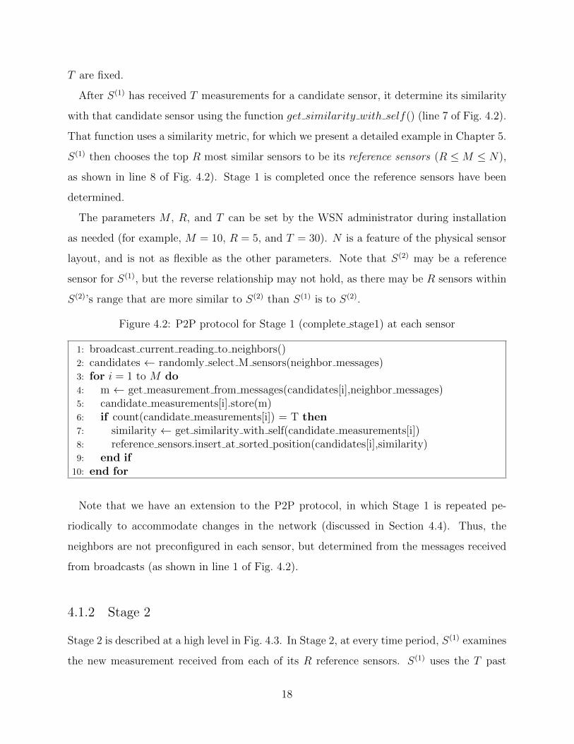
After S(1) has received T measurements for a candidate sensor, it determine its similarity
with that candidate sensor using the function get similarity with self() (line 7 of Fig. 4.2).
That function uses a similarity metric, for which we present a detailed example in Chapter 5.
S(1) then chooses the top R most similar sensors to be its reference sensors (R ≤M ≤ N),
as shown in line 8 of Fig. 4.2). Stage 1 is completed once the reference sensors have been
determined.
The parameters M , R, and T can be set by the WSN administrator during installation
as needed (for example, M = 10, R = 5, and T = 30). N is a feature of the physical sensor
layout, and is not as flexible as the other parameters. Note that S(2) may be a reference
sensor for S(1), but the reverse relationship may not hold, as there may be R sensors within
S(2)’s range that are more similar to S(2) than S(1) is to S(2).
Figure 4.2: P2P protocol for Stage 1 (complete stage1) at each sensor
1: broadcast current reading to neighbors()2: candidates ← randomly select M sensors(neighbor messages)3: for i = 1 to M do4: m ← get measurement from messages(candidates[i],neighbor messages)5: candidate measurements[i].store(m)6: if count(candidate measurements[i]) = T then7: similarity ← get similarity with self(candidate measurements[i])8: reference sensors.insert at sorted position(candidates[i],similarity)9: end if
10: end for
Note that we have an extension to the P2P protocol, in which Stage 1 is repeated pe-
riodically to accommodate changes in the network (discussed in Section 4.4). Thus, the
neighbors are not preconfigured in each sensor, but determined from the messages received
from broadcasts (as shown in line 1 of Fig. 4.2).
4.1.2 Stage 2
Stage 2 is described at a high level in Fig. 4.3. In Stage 2, at every time period, S(1) examines
the new measurement received from each of its R reference sensors. S(1) uses the T past
18

measurements to model the behavior of each of its reference sensors, using an approach
detailed in Chapter 5. If a sensor measurement from one of the reference sensors is found
to be anomalous as per that model (line 5 of Fig. 4.3), S(1) marks its own measurement as
anomalous. If S(1)’s measurement is found to be anomalous with respect to the majority of its
R reference sensors’ measurements, S(1) declares its own measurement as erroneous. S(1) then
immediately reports itself to the sink as faulty along with the erroneous measurement. If S(1)
has only two reference sensors, it reports the fault only if its measurement is anomalous with
respect to the measurements of both those reference sensors. The majority vote increases the
confidence in a fault report, and is a measure against false positives. A scenario is possible
in practice, although unlikely, wherein the majority of reference sensors are faulty, and the
sensor incorrectly marks itself as being faulty, following the majority. To enable investigation
in that scenario, when a sensor reports itself as faulty, it includes in that message a list of
all reference sensors that it used to find itself faulty (suspecting sensors). That allows a
network administrator to investigate those suspecting sensors (line 10 of Fig. 4.3).
Figure 4.3: P2P protocol for Stage 2 (complete stage2) at each sensor
1: broadcast current reading to neighbors()2: suspecting sensors ← empty queue()3: for reference sensor in reference sensors do4: r ← get measurement from messages(reference sensor,neighbor messages)5: if is anomalous(r,candidate measurements) then6: suspecting sensors.enqueue(reference sensor)7: end if8: end for9: if count(suspecting sensors) > count(reference sensors)/2 then
10: report fault to sink(current measurement,suspecting sensors)11: end if
4.1.3 Stage 3
Stage 3 happens at the sink after a sensor has asynchronously reported a fault in Stage
2. In this stage, the sink responds to the fault report by taking one of three decisions: 1)
commanding that sensor to serve purely as a forwarding node in a multi-hop network, 2)
19
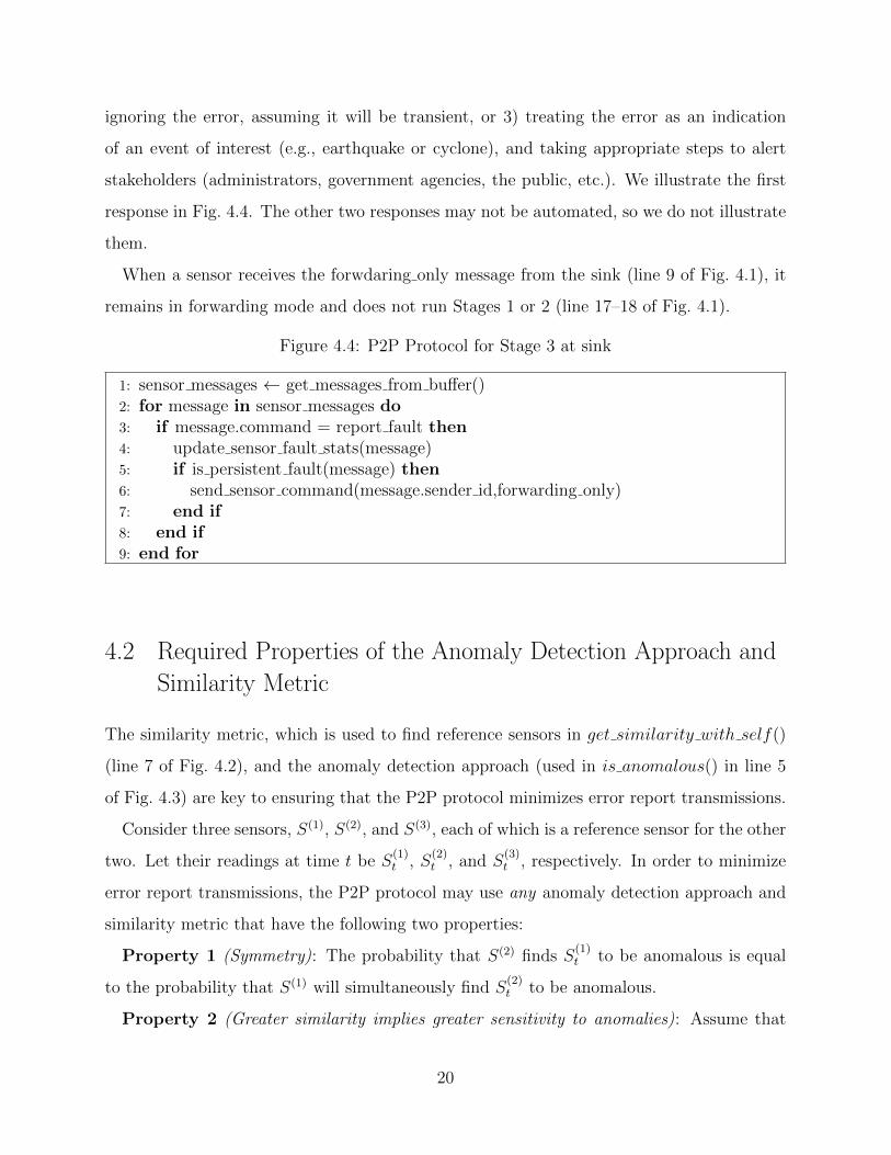
ignoring the error, assuming it will be transient, or 3) treating the error as an indication
of an event of interest (e.g., earthquake or cyclone), and taking appropriate steps to alert
stakeholders (administrators, government agencies, the public, etc.). We illustrate the first
response in Fig. 4.4. The other two responses may not be automated, so we do not illustrate
them.
When a sensor receives the forwdaring only message from the sink (line 9 of Fig. 4.1), it
remains in forwarding mode and does not run Stages 1 or 2 (line 17–18 of Fig. 4.1).
Figure 4.4: P2P Protocol for Stage 3 at sink
1: sensor messages ← get messages from buffer()2: for message in sensor messages do3: if message.command = report fault then4: update sensor fault stats(message)5: if is persistent fault(message) then6: send sensor command(message.sender id,forwarding only)7: end if8: end if9: end for
4.2 Required Properties of the Anomaly Detection Approach and
Similarity Metric
The similarity metric, which is used to find reference sensors in get similarity with self()
(line 7 of Fig. 4.2), and the anomaly detection approach (used in is anomalous() in line 5
of Fig. 4.3) are key to ensuring that the P2P protocol minimizes error report transmissions.
Consider three sensors, S(1), S(2), and S(3), each of which is a reference sensor for the other
two. Let their readings at time t be S(1)t , S
(2)t , and S
(3)t , respectively. In order to minimize
error report transmissions, the P2P protocol may use any anomaly detection approach and
similarity metric that have the following two properties:
Property 1 (Symmetry): The probability that S(2) finds S(1)t to be anomalous is equal
to the probability that S(1) will simultaneously find S(2)t to be anomalous.
Property 2 (Greater similarity implies greater sensitivity to anomalies): Assume that
20

the similarity between S(1) and S(2) is greater than the similarity between S(1) and S(3).
Then, the probability that S(2) will mark S(1)t as anomalous is greater than the probability
that S(3) will mark S(1)t as anomalous, because S(2) was more similar to S(1).
We prove energy-optimality assuming the above properties in Section 4.5, and present an
anomaly detection approach and similarity metric that have both properties in Chapter 5.
4.3 Memory Requirement
In all stages, each sensor stores T measurements broadcast by each of the M candidate sen-
sors. At each time period, a new measurement is stored and oldest of the T measurements is
discarded, so that the memory requirement is bounded to MT floating point measurements.
As a result, the memory requirement is O(MT ) = O(1), since M and T are fixed for a given
WSN. A typical experiment may have R = 3, M = 10, T = 300, and N = 200. Thus, the
memory requirement is well within low-cost sensor hardware capabilities.
4.4 Handling Changes in the Network
The WSN may change over time because of churn (in mobile settings) or changes in the
environment being monitored (resulting in a need for an updated model of sensor measure-
ment behavior). To account for those changes, the latest T measurements are refreshed after
a new set of M measurements (from the M candidate sensors) are received at every time
interval. Stage 1 of the protocol may be repeated, and a new set of R reference sensors may
be selected if the similarity rankings of the candidate sensors changed.
Instead of randomly selecting a new set of M candidates, Stage 1 as given in Fig.4.3 can be
modified as follows. The Q least similar sensors are occasionally removed from the candidate
sensor list and replaced with Q other randomly chosen sensors from the N −M neighbors,
where Q ≤M − R. This allows those Q other sensors to be given a chance to be chosen as
reference sensors. All that is implemented in place of line 1 of Fig.4.3. The remaining lines
of Fig.4.3 remain the same.
21
In order to accurately realize the energy-efficient protocol, it is necessary for the reference
sensors to represent the most similar sensors within a given sensor’s range.
4.5 Proof of Energy-Optimality
Many strategies for energy-optimized communication have been proposed that highlight the
importance of minimizing the number and length of messages to extend the lifetime of the
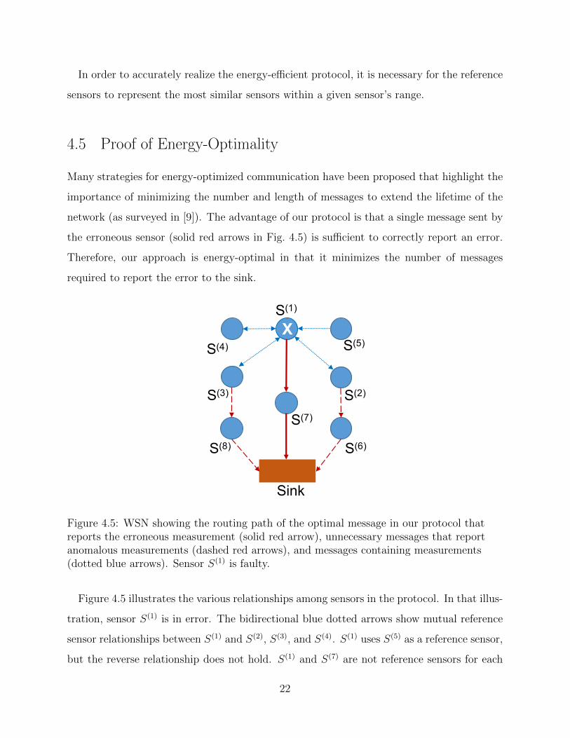
network (as surveyed in [9]). The advantage of our protocol is that a single message sent by
the erroneous sensor (solid red arrows in Fig. 4.5) is sufficient to correctly report an error.
Therefore, our approach is energy-optimal in that it minimizes the number of messages
required to report the error to the sink.
S(3) S(2)
S(4)
S(1)
Sink
S(6)
S(7)
S(8)
S(5)X
Figure 4.5: WSN showing the routing path of the optimal message in our protocol thatreports the erroneous measurement (solid red arrow), unnecessary messages that reportanomalous measurements (dashed red arrows), and messages containing measurements(dotted blue arrows). Sensor S(1) is faulty.
Figure 4.5 illustrates the various relationships among sensors in the protocol. In that illus-
tration, sensor S(1) is in error. The bidirectional blue dotted arrows show mutual reference
sensor relationships between S(1) and S(2), S(3), and S(4). S(1) uses S(5) as a reference sensor,
but the reverse relationship does not hold. S(1) and S(7) are not reference sensors for each
22

other, but S(7) is in S(1)’s shortest path to the sink.
Consider S(1), S(2), and S(3) in the example in Fig. 4.5. Let their readings at time t
be S(1)t , S
(2)t , and S
(3)t , respectively. Each sensor receives the readings from the other two
sensors at time t. Then, when S(1) exchanges its readings with S(2) and S(3), all three sensors
would immediately detect that there is an anomaly (by the two properties in Section 4.2).
In that situation, a suboptimal approach (such as the one in [6]) would have S(2) and S(3)
report the anomaly to the sink, leaving the sink to count votes and make a decision on the
error. That decision would affect not only the battery life of S(2) and S(3), but also that of
S(6) and S(8), which are on their respective routing paths to the sink. Another suboptimal
alternative would be for S(2) and S(3) to let S(1) know that they believe S(1)’s measurement
is anomalous, so that S(1) can then report its own error to the sink. While that approach
is significantly more energy-efficient than the previous one, it is still suboptimal. In our
approach, S(1) implicitly recognizes that S(2) and S(3) must have found it to be in error, and
it reports itself as erroneous to the sink.
It is obvious that at least one message must be necessary in order for S(1) to implicitly
recognize the fact that the majority of its 3 reference sensors found it to be anomalous.
The fact that one message is sufficient is not obvious, and is crucial in ensuring that the
protocol correctly reports the anomaly, while minimizing message transmissions (which is
the objective of this thesis). In order to show that one message is sufficient, we use Properties
1 and 2, as stated in Section 4.2.
Lemma 1. Assume that the similarity between S(1) and S(2) is greater than the similarity
between S(1) and S(3). Then the probability that S(1) would mark its own measurement as
anomalous with respect to S(2)’s measurement is greater than the probability that it would
mark its own measurement as anomalous with respect to S(3)’s measurement.
Proof. We know from Property 2 that, if S(1)t were anomalous, the anomaly would be recog-
nized with greater probability by S(2) than by S(3). From Property 1, we know that if S(2)
finds S(1)t to be anomalous, then S(1) would find S
(2)t to be anomalous with equal probability.
The Lemma follows.
Lemma 1 is phrased from the perspective of S(1) as it is detecting whether its own mea-
23

surement is anomalous with respect to measurements from S(2) and S(3) at time t. Also, it
follows that S(2) is the better sensor to be used by S(1) as a reference for anomaly detection,
because its greater similarity with S(1) implies greater sensitivity to anomalies.
Lemma 1 also highlights an important relationship detail. Consider S(1) and S(5) in
Fig. 4.5. S(1) uses S(5) as a reference sensor, meaning S(5) sends S(1) its measurements. S(5)
may not use S(1) as a reference sensor because it may have found other sensors that are more
similar to it. Therefore, S(5) does not consider whether S(1)t is anomalous at time t, but if
it did, and the similarity between S(1) and S(5) were greater than that between S(1) and
S(3), then it would have detected S(1)t as anomalous with greater probability than S(3) would
have (by Property 2). However, from Lemma 1, S(5) does not need to consider whether
S(1)t is anomalous at time t for S(1) to know that it did. As long as S(1) found S
(5)t to be
anomalous, we know that S(5) would have found S(1)t to be anomalous with equal probability
(by Property 1). Therefore the reference sensor relationship does not need to be a two-way
relationship for the protocol to work.
In [6], the authors suggest than any sensor that detects an anomalous measurement must
report the anomaly to the sink. However, that leads to unnecessary energy overhead for the
various sensors that detect the anomaly, and for the sensors on their multi-hop routing paths.
We now show that the erroneous sensor will recognize that other sensors have found it to be
anomalous without requiring those sensors to waste messages transmissions communicating
their knowledge of the anomaly.
Theorem 1. In the system model described in Section 2.1, let S(A) be a sensor whose
measurement at time t, S(A)t , is deemed anomalous by any neighboring sensor S(V ). Then,
the P2P error detection protocol, described in Section 4.1, ensures that S(A) will implicitly
recognize that S(A)t is anomalous with respect to that sensor’s measurement, S
(V )t .
Proof. If S(V ) is one of S(A)’s reference sensors, S(A) would evaluate its own measurements
with respect to S(V )’s measurements and will recognize that S(V ) found S(A)t to be anomalous
as soon as it finds that S(V )t was anomalous (by Property 1).
If S(V ) is not one of S(A)’s reference sensors, S(A) would not check its measurements against
S(V ), and will not know that S(A)t is anomalous with respect to S
(V )t . However, based on
24

how reference sensors are chosen, S(V ) not being one of S(A)’s reference sensors implies that
S(A)’s reference sensors are more similar to S(A) than S(V ) is to S(A). From Lemma 1, that
means that if S(A)t were anomalous with respect to S
(V )t , S
(A)t would also be anomalous with
respect to the measurements of all of S(A)’s reference sensors. In that scenario, although
S(A) is not checking its measurements against S(V ), S(A) will implicitly recognize that it is
anomalous using its reference sensors’ measurements.
Corollary 1. In the system model described in Section 2.1, consider a sensor that generates
a measurement that is deemed anomalous by the majority of that sensor’s reference sensors.
Exactly one message is sufficient to report the fact that the majority of multiple reference
sensors detected the anomaly.
Corollary 1 follows from Theorem 1, for if a sensor implicitly recognizes itself as erroneous,
it is not necessary for any sensor other than the erroneous sensor to report itself as erroneous
to the sink. We believe that this result is a major contribution of our work, combining results
from anomaly detection and routing theory in the design of an energy-optimal error detection
protocol that is easy to implement.
The path of the single message reported by erroneous sensor S(1) is given by the solid red
line in Fig. 4.5. That message is sufficient to capture the anomaly detected by the majority
of S(1)’s reference sensors. No other sensor is required to report the error, unlike in the
approach suggested in [6].
4.6 Main Strength and Limitation
The main strength of our approach lies in the fact that we minimize the number of messages
required to report an error to the sink. Exactly one message needs to be sent to the sink
when the network agrees that a sensor is in error, which happens when the majority of the
sensors most sensitive to an anomaly find that the sensor’s reading is anomalous.
The P2P protocol scales well to dense sensor networks where each sensor might have
several sensors within range to choose from. By controlling the parameter M described in
25

Section 4.1, the memory requirement for each sensor can be limited to order O(1), for fixed
M and T .
The P2P protocol can also be used in the context of mobile sensors, since we periodically
refresh the list of M candidate sensors from which R reference sensors are chosen.
The main limitation of our approach is the reliance of each sensor on the existence of
at least two similar sensors within its wireless communication range to serve as reference
sensors. For simplicity, we assume that reference sensors are always within one hop of the
sensor that is using them for reference. Since the one-hop distance implies spatial closeness
in a setting where sensors have a limited wireless communication range, it is assumed that
a sensor would find sufficient reference sensors to meaningfully vote on an error. However,
in a setting with isolated sensors or wireless signal barriers separating nearby sensors, our
protocol may not be able to find sufficient reference sensors to vote on an anomaly.
In order to address that limitation, the protocol can be trivially extended to allow sensors
to report their own measurements as erroneous, using their own past measurements for refer-
ence (without requiring any other sensor). Discussion of that extension is beyond the scope
of this thesis, but we provide a solution in [21]. That approach uses the Auto-regressive Inte-
grated Moving Average (ARIMA) model from past measurements to construct a confidence
interval to validate future measurements. The choice of confidence interval impacts detection
and false positive rates. Those rates can be controlled by setting appropriate thresholds set
for classifying measurements as anomalous. An Auto-regressive (AR) model alone may be
sufficient to detect anomalies at a computation cost much lower than that of the ARIMA
model. The computation cost is important to consider because running complex algorithms
on sensor hardware impacts the battery life.
26

CHAPTER 5
VALIDATION OF SENSOR MEASUREMENTS
In this chapter, we present a detailed description of an anomaly detection approach and an
associated similarity metric that satisfy both the properties required by our P2P protocol
(stated in Section 4.2). We use isocontours on a bivariate normal distribution to draw an
anomaly detection boundary, assuming that T measurements of two sensors have a joint
distribution that can be approximated by the normal distribution.
5.1 Summary of Approach
Consider two sensors SX and SY that take T measurements in T time periods. We seek
to determine whether a new measurement tuple (x, y) (from the two sensors SX and SY
respectively) is statistically consistent with the past T measurements taken by SX and SY .
The new measurement would typically arrive at time period T + 1.
Consider the simple model where SY sends all its measurements to SX . Let X and Y
denote the vector of the past T measurements from SX and SY respectively. Then SX
has both X and Y in its memory. Our assumption is that X and Y are jointly normally
distributed. Therefore, SX can create an isocontour from the jointly normal distribution to
define a region of normal and anomalous points.
For illustration (Fig. 5.1), we use two arbitrary sensors from the NZ dataset, and set
T = 300 to capture measurements during a 5 minute interval. In order to remove the effects
of having X and Y at different scales, and to simplify the anomaly detection procedure
(to meet low power constraints on sensors), we center the data and divide by the standard
deviation. That explains the range of the vertical and horizontal scales in the figure, and
why the isocontour is centered at the origin. The red point is an anomalous point (caused
27

5 0 5Sensor 16 Centered & Normalized
12
10
8
6
4
2
0
2
4
6
Senso
r 1
Cente
red &
Norm
aliz
ed
Figure 5.1: Single anomalous measurement (in red) in the NZ dataset is detected byconstructing an isocontour (blue shaded elliptical region) as a detection boundary. Normalmeasurements are inside the isocontour and are jointly Gaussian.
by an earthquake). Note that the measurement was not anomalous as per Sensor 16’s
measurements, but was anomalous as per Sensor 1’s measurements. That is explained in
Section 5.7, but for now we just point out that the anomalies are relative to the joint Gaussian
model of two sensors.
5.2 Anomaly Detection Approach Assumptions
The main assumptions for this anomaly detection approach are: 1) anomalies can lie any-
where in the two-dimensional vector space spanned by both sensors’ normalized measure-
ments, 2) anomalies lie farther away from the cluster centroid than proper measurements,
and in a manner that an elliptic isocontour can be used to separate them from proper mea-
surements (as shown in Fig 5.2), while maintaining an acceptable trade-off between true
positives and false positives, and 3) that elliptical isocontour must be centered at the cen-
troid of the proper measurements. The choice of the sliding window size, T , is crucial to
ensuring that these assumptions hold.
The reasoning behind our anomaly detection procedure applies to two sensors whose mea-
28

surements are jointly Gaussian. In practice, if they are jointly Gaussian, then detection
thresholds can be defined by well-known confidence intervals (or probabilities) for the Gaus-
sian distribution. If they are not strictly Gaussian, we may not be able to associate the
threshold with a confidence interval or probability. Even so, as along as the three afore-
mentioned assumptions hold, a valid detection boundary can be drawn using the approach
presented in this chapter.
5.3 Isocontours of the Bivariate Normal Distribution
The joint PDF of the Gaussian distribution for two random variables X ∼ N(µX , σ2X) and
Y ∼ N(µY , σ2Y ) is given as follows:
fX,Y (x, y) =1
2πσXσY√
1− ρ2exp− 1
2(1− ρ2)[CX,Y (x, y)] (5.1)
CX,Y (x, y) =(x− µX)2
σ2X
+(y − µY )2
σ2Y
− 2ρ((x− µX)(y − µY )
σXσY(5.2)
An isocontour is the equation of a hyperplane (in this case, a line) for which the joint
distribution has the same value (denoted by U). The equation of the isocontour can be
derived as follows:
fX,Y (x, y) = U (5.3)
⇒ 1
2πσXσY√
1− ρ2exp− 1
2(1− ρ2)[CX,Y (x, y)] = U (5.4)
⇒ CX,Y (x, y) =(x− µX)2
σ2X
+(y − µY )2
σ2Y
− 2ρ((x− µX)(y − µY )
σXσY= V (5.5)
V = −2(1− ρ2)log(2πσXσY√
1− ρ2U) (5.6)
Here, V is a constant (a function of U , which is also a constant). Thus, CX,Y (x, y) defines
the equation of an ellipse centered at (µX , µY ) at an angle with respect to the X and Y axes.
Clearly, it would be very complicated and computationally expensive to compute CX,Y (x, y)
29

in the above form. This motivates a simplified approach.
5.3.1 Simplified Isocontours of Two Uncorrelated Gaussians
If we were to assume that X and Y were already centered uncorrelated, then µX = µY =
ρ = 0, and Eqn. (5.6) simplifies to
CX,Y (x, y) =x2
σ2X
+y2
σ2Y
= V (5.7)
V = −2log(2πσXσYU) (5.8)
In addition, let us find the isocontour with the value U such that U is k standard deviations
from the mean. Then,
U = fX,Y (kσX , kσY ) =1
2πσXσYexp−1
2[CX,Y (kσX , kσY )] (5.9)
Substituting into V in Eqn. (5.8), we get
CX,Y (x, y) =x2
σ2X
+y2
σ2Y
= CX,Y (kσX , kσY ) = 2k2 (5.10)
This is a much simpler isocontour of an ellipse that is parallel to the X and Y axes, centered
at the origin with major/minor radii given by√
2σX and√
2σY .
5.3.2 Obtaining the Simplified Isocontour
The first step in obtaining the simplified isocontour is to center the data by subtracting the
means from both X and Y . The second step is to obtain a transformation matrix such that
the transformed data is uncorrelated. That transformation matrix is obtained as follows.
Let A =[X Y
]be a T × 2 matrix containing the data. Then the 2× 2 covariance matrix
for X and Y is given as follows:
A′A
T − 1=[ V ar(X) Cov(X,Y )Cov(Y,X) V ar(Y )
](5.11)
30

The covariance matrix is symmetric because Cov(X, Y ) = Cov(Y,X). We want to estimate
the matrix E that performs the following transformation:
AE = A∗ (5.12)
where A∗ =[X∗ Y ∗
]is a T × 2 projection of A, and has uncorrelated columns X∗ and Y ∗.
If Cov(X, Y ) = 0, there is nothing further to be done because A = A∗, and we can directly
apply the simplified isocontour Eqn. (5.10).
Cov(X, Y ) 6= 0, we are effectively interested in rotating the measurements into a new axis
where the covariance is zero. That is obtained by Principal Component Analysis (PCA),
which states that the orthonormal eigenvectors of the covariance matrix rotate the original
data into the principal component space where the data is uncorrelated. After applying
PCA, we get the covariance matrix of A∗ as
(A∗)′A∗
T − 1=[L1 00 L2
](5.13)
where L1 and L2 are the eigenvalues of A′A/(T −1), and represent the variance in the direc-
tion of the new space spanned by the eigenvectors given by the columns of E in Eqn. (5.12).
To show that E is the matrix that produces X∗ and Y ∗ that are uncorrelated, consider the
following:(A∗)′A∗
T − 1=
(AE)′(AE)
T − 1=E ′(A′A)E
T − 1(5.14)
From the definition of eigenvectors E =[E1 E2
]and eigenvalues L =
[L1 00 L2
], of the
matrix CA = A′AT−1 ,
CAE = EL (5.15)
⇒ E−1CAE = L (5.16)
That is a simple proof of one of the basic principles from Linear Algebra, called the diagonal-
ization of CA. Noting that by orthonormality, E ′ = E−1, we can substitute into Eqn. (5.14)
31

8 6 4 2 0 2 4 6 8Sensor 16 Centered & Normalized
8
6
4
2
0
2
4
6
Senso
r 1
1 C
ente
red &
Norm
aliz
ed
8 6 4 2 0 2 4 6 8Larger Principal Component
8
6
4
2
0
2
4
6
Sm
alle
r Pri
nci
pal C
om
ponent
Figure 5.2: Anomalies (red crosses) in the NZ dataset due to earthquake observed innormalized measurement space (left) and the space spanned by the two principalcomponents (right).
to get the following:
(A∗)′A∗
T − 1=E ′(A′A)E
T − 1=E−1(A′A)E
T − 1= L (5.17)
where L is a diagonal matrix containing the eigenvalues of A′A. Therefore (A∗)′A∗
T−1 is diagonal,
and the columns of A∗, which are X∗ and Y ∗, are thus uncorrelated. X∗ and Y ∗ represent
the principal components in the orthogonal subspace Fig. 5.2 (right plot), while X and Y
represent the points in the original space of sensor measurements (left plot).
With these new uncorrelated vectors in the new principal component space, we can apply
Eqn. (5.10). Note that we cannot apply that equation directly on X and Y when they are
correlated.
CX∗,Y ∗(x∗, y∗) =
(x∗)2
σ2(X∗)
+(y∗)2
σ2(Y ∗)
= 2k2 (5.18)
Note that in order for this to work, we had to rotate not only X and Y , but also the
test data point (x, y) to get (x∗, y∗). The rotation was obtained from the transformation E,
32

resulting in the points being aligned in a way that the direction of maximum variance is in
line with the horizontal axis. This is illustrated for two sensors in the NZ dataset in Fig. 5.2.
5.3.3 Calculating the Angle of Rotation
The data X and Y was rotated in the 2-D space to produce X∗ and Y ∗ which were un-
correlated. Note that X and Y are to some extent blended together in X∗ and Y ∗. So in
the new principal component space (Fig. 5.2 (right)), X∗ and Y ∗ do not directly correspond
to the original sensor measurements, but to some blend of the measurements. This rota-
tion was performed purely for mathematical simplification, which in turn leads to efficient
computation.
The ellipse CX∗,Y ∗ is essentially the rotation of the ellipse CX,Y . The angle of rotation
describes the angle of the rotated ellipse with respect to the axes of the original ellipse.
Calculating the angle of rotation is not useful for anomaly detection, but we present it here
for completeness of the mathematical intuition. We used this approach in plotting the ellipse
in the figures because the plotting tools required the angle to be specified as a parameter.
Let us give names to the elements of E. Let E =[e00 e01e10 e11
]. And let θ be the angle of
rotation. Then there is a one-to-one correspondence between the elements of E and the
rotation matrix.
E =[e00 e01e10 e11
]=[cos θ − sin θsin θ cos θ
](5.19)
⇒ θ = arctan(e10/e00) (5.20)
In implementing the function in code, one must note that it is possible (though in our
applications highly unlikely) that e00 = 0, leading to a divide by zero error. That simply
means that θ = 90 (if e10 > 0) or θ = 270 (if e10 < 0). The Numpy library in Python has
a function called arctan2 which is an alternative to arctan, and takes care of those special
cases.
33

5.4 Anomaly Detection Procedure
In this section, we explain the algorithm that goes into is anomalous(), the function used
in Stage 2 of the P2P protocol in line 5 of Fig. 4.3. If Sensor SX receives all measurements
from sensor SY , then SX can determine whether a particular reading of SY was anomalous.
Let the test reading be y and have a corresponding reading x measured by SX at the same
time period. SX builds a model of SY ’s measurements using T measurements from the past.
If y was found to be anomalous as per that model, then SX declares y to be in error. The
model we use is the bivariate normal distribution described in Section 5.3.
Let X be the past T measurements of SX and Y be the past T measurements of SY .
Let ← denote the assignment operator. In summary, the anomaly detection approach is
composed of the following steps:
1. Center the data for numerical simplicity so that the scatter plot is centered at the
origin. Here data refers to both the historic measurements X and Y as well as the test
point (x, y)
X ← X − µX Y ← Y − µY (5.21)
x← x− µX y ← y − µY (5.22)
2. Normalize the data by dividing by standard deviation. This ensures that the difference
in scale of magnitudes does not matter. For example, a sensor that is located closer
to a region of large seismic activity (a volcano, for example) may have an amplitude
much greater than that of a farther away sensor. We want to remove that amplitude
disparity because that allows us to give equal weight to anomalies in the direction of
both sensors. If we had not done that, a deviation in the direction of the sensor that
measures a larger amplitude would automatically be weighted more than a deviation
in the direction of the smaller amplitude. Normalization also takes care of the fact
that some sensors may not be calibrated to have a standard unit (like the cast of all
34

our NZ data).
X ← X/σX Y ← Y/σY (5.23)
x← x/σX y ← y/σY (5.24)
As a consequence of this step, σX = σY = 1.
3. Compute the covariance matrix CA of X and Y , as explained in Eqn. (5.3).
A←[X Y
](5.25)
CA ←A′A
T − 1(5.26)
4. Compute the orthonormal eigenvectors E and eigenvalues L of CA. A computationally
simple way of doing this is presented in Section 5.4.1.
E,L← eig(CA) (5.27)
The diagonal elements of L give the variance in the rotated space. L =[ σ2
(X∗) 0
0 σ2(Y ∗)
]5. Transform the test point into the principal component space given by E.
[x∗ y∗
]←[x y
]E (5.28)
6. For a given detection threshold k, the point test point (x, y) is anomalous if the fol-
lowing condition holds, as explained in Eqn. (5.18):
(x∗)2
σ2(X∗)
+(y∗)2
σ2(Y ∗)
> 2k2 (5.29)
35

5.4.1 Cost-efficient Computation of Orthonormal Eigenvectors andEigenvalues
While designing the validation approach for a peer-to-peer validation mechanism, it is im-
portant to consider the computation cost of validation. In this subsection we show that
the above detection scheme can be computed with very simple addition and multiplication
operations.
For a 2x2 covariance matrix, the eigenvectors and eigenvalues can be computed using the
following simple Python code. Note that no library functions were called other than the sqrt
(square root function).
1 import numpy as np
2 de f e i g (X) :
3 D = X[ 0 , 0 ] ∗X[1 ,1 ]−X[ 0 , 1 ] ∗X[ 1 , 0 ]
4 Tr = X[0 ,0 ]+X[ 1 , 1 ]
5 L1 = Tr/2 .0 + np . sq r t (Tr∗∗2/4.0 −D)
6 L2 = Tr/2 .0 − np . sq r t (Tr∗∗2/4.0 −D)
7 i f X[ 1 , 0 ] != 0 :
8 E1 = np . matrix ( [ L1−X[ 1 , 1 ] , X[ 1 , 0 ] ] ) . reshape (2 , 1 )
9 E2 = np . matrix ( [ L2−X[ 1 , 1 ] , X[ 1 , 0 ] ] ) . reshape (2 , 1 )
10 E1 = E1/np . l i n a l g . norm(E1)
11 E2 = E2/np . l i n a l g . norm(E2)
12 e l s e :
13 E1 = [ 1 , 0 ]
14 E2 = [ 0 , 1 ]
15 re turn np . array ( [ L1 , L2 ] ) , np . hstack ( [ E1 , E2 ] )
Listing 5.1: A simplified implementation of the eig function
Note that the matrix X in the above example must be symmetric (a property inherent to
covariance matrices). Therefore X[0, 1] = X[1, 0], and the first condition checks to see if the
matrix is a diagonal matrix. If it is a diagonal matrix, it means that the two sensors were
uncorrelated to begin with. Hence there is no need to transform them onto a space where
they are uncorrelated, and the transformation matrix is the identity matrix.
We now explain the mathematics of the code. Let X =[a bc d
]. By definition of eigenvectors
36

(E) and eigenvalues (L),
Xv = λv ⇔ (X − λI)v = 0 (5.30)
where v is a 2 × 1 eigenvector, λ is a scalar eigenvalue, and I is the 2 × 2 identity matrix.
In order for Eqn. (5.30) to have a non-trivial solution, we require
det(X − λI) = 0⇒ det([a−λ bc d−λ
]) = 0 (5.31)
⇒ λ2 − (a+ d)λ+ (ad− bc) = 0 (5.32)
where det is the determinant function. Let the D = det(X) = ad−bc and Tr = tr(X) = a+d
(these are defined in lines 3 and 4 of Code 5.1). The two eigenvalues can be obtained by
solving the quadratic Eqn. (5.32), and the solutions are given in lines 5 and 6 of Code 5.1.
Let the first eigenvector E1 =[e00e10
]have the corresponding eigenvalue L1. Then, from
Eqn. (5.30),
ce00 + (d− L1)e10 = 0⇒ e00e10
=(L1− d)
c(5.33)
Since we require orthonormal vectors, E1 is the normalized (by L − 2 norm) form of the
vector[(L1−d)
c
]. This is given for E1 (and similarly for E2) in lines 8 to 11 of Code 5.1.
Note that this solution is only valid in the case where X[1, 0] = c 6= 0 because of the
division by c in Eqn. (5.33). The eigenvectors are combined into a transformation matrix
E = [E1, E2] =[e00 e01e10 e11
]Note that lines 8 to 11 of Code 5.1 can be collapsed into a single line of Python code, but
we have separated them here for better readability. Our separation of code explains how the
eigenvectors are related to their eigenvalues.
37

5.4.2 Algorithm Complexity
Since the anomaly detection approach is executed on low-cost sensor hardware, it is essential
that the implementation be simple and memory requirements be minimal. The computations
in Steps 1–3 of the procedure in Section 5.4 are all O(T ), and Steps 4–6 are O(1). Since the
procedure is repeated for R reference sensors, the total algorithm complexity is O(RT ) =
O(1) since R and T are fixed for a given WSN.
5.4.3 Robustness of Implementation
When we say that X and Y contain the past T measurements taken by sensors SX and SY ,
we mean the past T normal measurements. Therefore, if a test measurement (x, y) is found
to be anomalous, it is discarded from the model. This ensures that the model is robust and
cannot easily become biased due to outliers. If the anomalies were included in the model,
the area of the isocontour would effectively increase, and measurements that were earlier
flagged as anomalous may no longer be flagged as anomalous as they may now fall within
the isocontour.
5.5 Similarity Metric
We say that the measurements of two sensors are similar if they are tightly clustered in the
2-dimensional space. That tight clustering may be defined in many ways, but we use the
area of the kσ isocontour to determine how similar two sensors are. Mathematically, the
degree of similarity is expressed as the area of the ellipse in Eqn. (5.18). That is given as
follows:
Similarity(SX , SY ) = [2πk2σ(X∗)σ(Y ∗)]−1 (5.34)
5.5.1 Computation of Similarity Metric
The formula given in Eqn. (5.34) is the correct formula to calculate the area of the ellipse,
and is a perfectly valid similarity metric. The purpose of the similarity metric, however,
38

is for a sensor to compare its similarity to other sensors and obtain an ordering of similar
sensors from which it can obtain its reference sensors. Consider three sensors SX , SY , SZ .
If SY is more similar to SX than SZ is to SX ,
[2πk2σ(X∗)σ(Y ∗)]−1 < [2πk2σ(X∗)σ(Z∗)]
−1 ⇒ [σ2(X∗)σ
2(Y ∗)]
−1 < [σ2(X∗)σ
2(Z∗)]
−1 (5.35)
The above relationship is valid because we use the same value for k across all sensors to
define a threshold. Therefore, we can define an equivalent similarity metric (for ranking
purposes) as follows:
Similarity(SX , SY ) = [σ2(X∗)σ
2(Y ∗)]
−1 (5.36)
Computing the formula in Eqn. (5.36) is more efficient than computing the formula in
Eqn. (5.34) because we already had L1 = σ2(X∗) and L2 = σ2
(Y ∗) from the two eigenvalues of
the covariance matrix of[X Y
]. So we simply take their product, and skip taking the square
root and other operations. Also note that this version of the similarity metric is independent
of the anomaly detection threshold k.
5.6 Demonstrating Required Properties of Approach
This approach has two properties that are critical to our design of the P2P validation pro-
tocol. The two properties were assumed in the analysis of the protocol in Section 4.5 when
proving that our approach can achieve the minimum number of messages that need to be sent
in order to report the error. We now show that our approach satisfies those two properties,
and is thereby suitable for the protocol.
5.6.1 Symmetry
In this subsection, we show that our anomaly detection approach satisfies Property 1, as
stated in Section 4.2.
In Section 5.4, we assumed that Sensor SX receives all measurements from sensor SY and
39

performs anomaly detection. If we also assumed that Sensor SY receives all measurements
from sensor SX , then the question is whether or not the same pair (x, y) would be determined
as anomalous by SY .
Symmetry is not always guaranteed by anomaly detection approaches (see Appendix A.1
for an example of an approach that fails to provide symmetry). Let X and Y be centered
and normalized measurements of two sensors SX and SY . When SX performs anomaly
detection, it constructs the matrix in Step 3 of Section 5.4 as A ←[X Y
]. SY would
similarly construct the matrix as A ←[Y X
]. In order to show symmetry, we now show
that this construction leads to the same condition for anomaly detection in Eqn. (5.29). We
use the ‘hat’ notation to distinguish the results of the A construction.
Notice that the following column swap elementary transformation can be used to relate A
and A
A = A
0 1
1 0
, A = A
0 1
1 0
(5.37)
The corresponding covariance matrix is given as follows:
CA ←A′A
T − 1(5.38)
(5.39)
Substituting from Eqn. (5.37),
CA =
0 1
1 0
A′A0 1
1 0
T − 1
=
0 1
1 0
CA0 1
1 0
(5.40)
CA =
a b
c d
⇒ CA =
d c
b a
(5.41)
Note that the characteristic equation for CA is identical to the equation for CA given in
Eqn. (5.32). Therefore, the eigenvalues are exactly the same, except that we must name the
40

larger of the eigenvalues as σ∗Y .
σ∗Y = σ∗X (5.42)
σ∗X = σ∗Y (5.43)
The equation for computing eigenvectors and eigenvalues of CA is given as follows:
CAE = EL (5.44)
where CA, E and L are all 2× 2 matrices. L is a 2× 2 diagonal matrix of eigenvalues. We
showed that L = L. Similarly we can apply Eqn. (5.33) to show that E =
0 1
1 0
E.
In Step 4. of Section 5.4, SX rotated the test point[x y
]as follows:
[x∗ y∗
]←[x y
]E (5.45)
Similarly, SY would rotate the test point[y x
]as follows:
[y∗ x∗
]←[y x
]E =
[y x
]0 1
1 0
E =[x∗ y∗
](5.46)
Combining the above equation with Eqn. (5.43), we obtain the anomaly detection equation
for SY , which is the same as it is for SX in Eqn. (5.29).
5.6.2 Greater Similarity Implies Greater Sensitivity to Anomalies
In this subsection, we show that our similarity metric (described in Section 5.5) satisfies
Property 2, as stated in Section 4.2.
Let Similarity(SX , SY ) > Similarity(SX , SZ) for some sensors SX , SY , and SZ . From the
definition of the similarity metric in Eqn. (5.34), the area of the isocontour spanned by the
normalized measurements of SX and SY is smaller than the corresponding area spanned by
41

the normalized measurements of SX and SZ . With the assumption that anomalies are spread
out farther away from the centroid than are proper measurements, SX is more likely to detect
anomalies if it were to choose SY instead of SZ as a reference sensor because anomalies are
more likely to fall outside the smaller isocontour formed by SX and SY . Hence Property 2
is satisfied.
Note that if the area of the isocontour is smaller, more anomalies will be detected, but
also more false positives may result. If the area is larger, fewer anomalies will be detected,
but there would also be fewer false positives. Therefore, an appropriate threshold k must be
set to a good trade-off between true and false positives. In all our experiments, we set k = 3
and found that it achieves a perfect detection rate for all sensors and a zero false-positive
rate.
5.7 Illustration of Approach on Datasets
In this section, we demonstrate anomaly detection approach and also demonstrate important
features of the similarity metric on our three datasets. For the Berkeley dataset we use
T = 30, grouping 30 hours of data in one cluster. For the TAO dataset we use T = 30,
grouping 5 hours of data in one cluster. For the NZ dataset we use T = 300, grouping 5
minutes of data in one cluster.
5.7.1 Detecting Anomalies in the Datasets
In this subsection, we demonstrate our anomaly detection approach on all three datasets.
Consider the two sensors Sensor 1 and Sensor 16 in the NZ dataset. In Fig. 5.1, it can
be seen that the anomalous point is only anomalous with respect to Sensor 1 and not with
respect to Sensor 16. That is because Sensor 16 measured the earthquake later than Sensor 1
did. The waveforms along with anomalies flagged by the approach are illustrated in Fig. 5.3,
and the lag between Sensor 1 and Sensor 16 detecting the quake is clear in Fig. 5.3.
We also experimentally verified that our anomaly detection approach does indeed have
the symmetric property. From Sensor 1’s perspective, 67 anomalies were discovered in 86400
42

measurements during the 24 hr period with respect to Sensor 16’s measurements. Conversely,
from Sensor 16’s perspective, 67 anomalies were discovered during that period with respect
to Sensor 1’s measurements and those anomalies were reported at the exact same time indices
as those reported by Sensor 1. Note that each of the two sensors are performing anomaly
detection independent of the other. That is, the fact that one sensor finds the other sensor
to be anomalous is in no way communicated to the other sensor. Therefore the probability
of the two sensors having the exact same match in this case is 6× 10⁻⁷. That highly precise
match was expected because we know that symmetry is mathematically supported.
The 67 anomalies detected from the 86400 measurements were a result of the robust
anomaly detection approach discussed in Section 5.4.3. If the robust approach were not
used, we found from experiments that 33 anomalies would have been detected in the same
time period. That is because the initial anomalies would bias the model in a way that makes
future anomalies seem normal. That is, the isocontour would be expanded to accommodate
the initial anomalies in the model, leading to a wider range of what is normal.
10000
5000
0
5000
10000
Seis
mic
Am
plit
ude
Sensor 16
Relative Anomalies
00:06:5101/04
00:07:2101/04
00:07:5101/04
00:08:2101/04
00:08:5101/04
00:09:2101/04
00:09:5101/04
Time/Date in January 2016
200000
100000
0
100000
200000
Seis
mic
Am
plit
ude
Sensor 1
Relative Anomalies
Figure 5.3: Anomalies (yellow stars) due to the earthquake presented in the seismicwaveform in the NZ Dataset (200 sec view).
Figure 5.3 highlights that it is not necessary for both sensors to produce anomalous mea-
43

15 10 5 0 5 10 15 20Sensor 1 Centered & Normalized
5
0
5
10
15
20
25
30
35
Senso
r 13 C
ente
red &
Norm
aliz
ed
(a) Berkeley- Isocontour drawn atk = 75
400 300 200 100 0 100 200 300 400Sensor 1 Centered & Normalized
700
600
500
400
300
200
100
0
100
Senso
r 2
Cente
red &
Norm
aliz
ed
(b) TAO- Isocontour drawn atk = 500
3000 2000 1000 0 1000 2000 3000Sensor 1 Centered & Normalized
6000
5000
4000
3000
2000
1000
0
1000
Senso
r 7
Cente
red &
Norm
aliz
ed
(c) NZ- Isocontour drawn at k = 75
Figure 5.4: Anomalies (red crosses) in the three datasets are egregious. They would bedetected even if the isocontour were drawn 75, 500 and 3600 standard deviations from themean in the Berkeley, TAO and NZ datasets, respectively.
surements at the same time for the anomaly to be detected. Since anomalies are detected in
pairs of sensor measurements, it can be seen in Fig. 5.3 that at times anomalies are due to
Sensor 1’s measurements and at other times anomalies are due to Sensor 16’s measurements.
In order to ascertain which sensor is actually in error, we invoke the majority voting proce-
dure described in the protocol in Chapter 4. If a sensor believes its own reading is anomalous
based on the measurements taken at the same time by the majority of its reference sensors,
it will report itself as being in error to the sink.
An important point to notice in Fig. 5.2 is that there are points that are not anomalous
with respect to either Sensor 11 or Sensor 16. They are anomalous with respect to the
joint distribution of both sensors’ measurements. In other words, if the region capturing
normal consumption were rectangular, those anomalies would not be detected. They are
only detected because the region is elliptical. Since we did want to capture those anomalies,
the elliptical isocontour captured the detection boundary better than a rectangular region
would have.
In all three datasets, the anomalies due to errors were so egregious that our approach easily
detected them. Centering the data in the TAO dataset caused the anomalous points at −9.99
C to go further negative (to approximately −35 C), where the correct measurements were
around the origin. Dividing that by a fractional standard deviation further exaggerated
44

the anomaly to the extent that it would be detected even if the isocontour were drawn 500
standard deviations from the mean. Similarly, the errors in the Berkeley and NZ dataset
could be detected by isocontours drawn at 75 and 3600 standard deviations from the mean,
respectively. As shown in Fig. 5.4 for all three datasets, the anomalies due to errors were so
egregious that they could be easily distinguished from legitimate rare events. For example,
in the NZ dataset, a k = 3600 isocontour could detect an anomaly caused by a fault, but
it would have been too large to detect an earthquake. A k = 3 isocontour would detect
errors due to faults and earthquakes. Using both isocontours, the two errors types can be
differentiated.
5.7.2 Similarity Metric and Physical Distance
In this section we illustrate the relationship between the similarity metric and physical
distance in our dataset. Recall that we had analyzed the properties of the similarity metric
in relation to the protocol in Section 4.1.
Consider the 4 location markers in the largest circle in the top left of Fig. 5.5. Those
sensors are located around a volcano. We picked one of those sensors, and ranked the
similarity of all 40 other sensors in the dataset with that sensor (let us refer to it as SX).
The 41 sensors were located all around the country of New Zealand including small islands
(like Chatham Island). Of those 41 sensors, 5 are marked with smaller circles in the figure,
to avoid confusion with the other highway symbols shown by Google Maps.
Our first observation is important to show that our choice of similarity metric (explained
in Section 4.2) works for our protocol. That observation is that the top 3 sensors on the
ranked list of sensors were the nearest three at that same volcano as SX . Therefore, our
similarity metric picked the sensors that were physically closest to the one being considered.
We believe that it is because the sensor readings are from an almost identical distribution.
Our second observation is that the normalizing constant used in normalizing the sensor
data before deriving the similarity metric cannot be arbitrarily chosen (Step 3 of the anomaly
detection approach in Section 5.4). To test the effect, we normalized the data by the L− 2
norm of the T measurement values, instead of the standard deviation. We found that the
45

Figure 5.5: Map of physical location of select seismic wave sensors in the NZ dataset. Thefour sensors grouped in the largest circle are located around a volcano.
resultant similarity metric produced a ranking that had arbitrary sensors in the top 3 for
SX , none of which were at the volcano. That is because the standard deviation preserves
properties of the original distribution that the L− 2 norm does not.
Our third observation is that the ranking (using the standard deviation) outside of the
top 3 is not really indicative of physical distance. For instance, SX ’s similarity with the
sensor at the top right of Fig. 5.5 is less than the similarity with the sensor at the bottom
right of the figure. despite the fact that the sensor at the top right is clearly closer to SX .
We believe that this is because of two reasons. First, the sensors farther away from the
volcano belonged to a different seismic network maintained by a different organization, and
therefore the data collection and calibration methods might have been different. The sensors
at the volcano all belonged to the same network. Second, the location of the sensor, with
respect to the surface terrain might have affected the readings. Those effects might be due
46

to the way winds blow or other geological factors. The sensors at the volcano, on the other
hand, were all on the same hill so similar to each other. Third, external disturbances due to
moving vehicles, animals, machinery, etc., may create different amounts of noise at different
locations.
The conclusion is that the similarity metric captures physical distance only within a local
area. Outside of that area, no guarantees can be made on the relationship between similarity
and physical distance. That does not necessarily hurt our approach because each sensor is
only identifying reference sensors within its wireless range which is inherently restricted to
a local area.
47

CHAPTER 6
PROTOCOL EVALUATION
We evaluated the centralized and P2P validation protocols using our own implementation
of the protocols in a trace-driven simulator. In this section, we present the simulator and
our simulation results. The simulator allows us to quantify the longevity and reachability
of the network, when using the centralized and P2P protocols. Longevity and reachability
are the two metrics we care about, and were defined in Chapter 2. Our results show that
the P2P protocol described in Chapter 4 increases longevity and reachability, highlighting
its usefulness. The simulations are performed on the three datasets described in Chapter 3.
6.1 Sensor Network Protocol Simulator
Several simulators exist for modeling WSNs, as described in [22]. However, those simulators
either fail to conveniently support the implementation of P2P validation on top of existing
functionality, or fail to capture the impact of various sensor actions on battery consumption.
NS-2 [23] is a general-purpose network simulator that is targeted towards IP networks, but it
does not consider power consumption or cost metrics for energy-efficient routing as adjustable
parameters. TOSSIM [24] is an emulator specifically for TinyOS sensors developed by the
TinyOS project team, but it suffers from many of the same limitations [22]. To focus on
the application and routing layers of the network stack in developing an energy-efficient
P2P validation protocol, we developed a trace-driven simulator of a WSN in Python. The
simulator performs shortest-path routing and implements the application-layer protocols for
both centralized and P2P validation.
48

6.1.1 Simulator Design
The simulator is logically divided into three components: 1) the simulation engine that
bootstraps the simulation, 2) the sensor class that contains the code that would run on
sensor motes, and 3) the sink class that contains the code that would be executed at the
sink (on a server at the base station). The components are illustrated in Fig. 6.1.
SIMULATIONENGINE
SENSORCLASS SINKCLASS
CommunicationModule
EventManager
RoutingManager
AnomalyDetectionModule
MainModule
CommunicationModule
AnomalyDetectionModule
MainModule
InputParser
EventLogger
Figure 6.1: Components of the custom-built discrete event simulator.
In the P2P protocol implementation, the sensor class implements all three stages of the
protocol, described in Section 4.1. In the centralized implementation, the sensor class simply
sends all measurements to the sink at every time period, so that the sink may perform
anomaly detection in real-time. In both the centralized and P2P protocol implementations,
the sink class implements Stage 3 of the protocol, as described in Fig. 4.4.
Both the sensor and the sink classes contain a communication module that handles the
application and routing layer protocol messages, an anomaly detection module that imple-
ments the mechanism described in Chapter 5, and a main module that coordinates the other
two modules as per the protocol. On the sink, anomaly detection is performed with respect
to reference sensors that may be chosen from any sensor in the network (not limited to the
wireless range of each sensor). We obtain the top 5 reference sensors for each sensor when
performing anomaly detection at the sink.
The simulation engine contains an input parser, event manager, routing manager and
49

event logger. The input manager parses datasets and sensor layout description files (con-
taining spatial coordinates of sensors). The event manager stores and runs synchronous and
asynchronous events performed by the sensor and sink. Synchronous events include mea-
surement reading and reporting. Asynchronous events are communication events relating to
error reports. The sensor and sink class communicate with each other through the routing
manager in the simulation engine, which reads and writes to message buffers in the sensor
and sink classes. The routing manager implements static and time-varying routing protocols
to route messages between sensors and the sink. The event logger is used by the sensor and
sink classes to records statistics that allow us to trace the trajectory of the simulation and
evaluate performance metrics for different experiments.
6.1.2 Simulation Parameters
The simulator contains several configurable parameters that describe WSN settings. Lo-
cation coordinates are one such parameter, and they describe the physical locations of the
sensors and the sink. We place sensors in a 2-dimensional coordinate space for illustrative
simplicity, although we note that the implementation can be trivially extended to support
a 3-dimensional space. The second set of parameters describes the energy consumption of
the sensor motes in the network. We categorized CPU processes into long and short pro-
cesses. Long processes occur only in the P2P validation protocol (where the processing onus
is on the sensors), causing more battery drain due to CPU than in the centralized validation
protocol.
For the evaluation in this thesis, we assumed the use of the Mica2Dot sensors with weather
boards deployed at the Intel Berkeley Research Lab [2]. We obtained values for the energy
consumption of the CPU, radio transmission and radio receive from the third-generation
Mica2Dot sensor datasheet [25], and note that the choice of those values can have a major
effect on the evaluation results. The values for the Berkeley dataset deployment are presented
in Table 6.1.
In order to complete the simulation in reasonable time, we scaled down the battery capacity
of the sensors. For simplicity, we assume that the time at which sensors die will scale
50

linearly with increased battery capacity. We believe that is a reasonable assumption given
homogeneous sensor hardware. We leave a simulation time scaling analysis for future work.
We assume the same time scaling factor given in Table 6.1 for all three datasets deployments.
That assumption is reasonable if we also assume the following: if the sensor transmitter
hardware consumes more power in one deployment, then that deployment is equipped with
proportionately greater battery capacity.
The sensor battery capacity in the simulation (0.2 mAh) corresponds to 4 button cells of
200 mAh each1. We include a correction factor to account for battery capacity degradation
(due to imperfect battery quality or environmental effects), and to account for sensor activ-
ities that we did not carefully model (such as the idle state when asleep). Therefore, we say
the effective battery life of four button cells is reduced from 800 mAh to 666 mAh (a reduc-
tion of nearly 18%. In each time step, all alive sensors broadcast their readings to neighbors
within their wireless transmission range. By diving all times shown in the results and plots
by the time scaling factor given in Table 6.1, one can obtain the number of simulation time
steps that were run.
6.2 Protocol Implementation
In the centralized validation protocol, the sensors report their measurements to the sink at
every time epoch. These messages are forwarded by sensors that lie between the sender
and the sink. Upon receiving each measurement, the sink performs anomaly detection, as
described in Chapter 5.
In the P2P validation protocol, the sensors broadcast their measurements to their one-hop
neighbors at every time epoch. Each sensor determines whether its own measurement is in
error with regard to measurements from its reference sensors. If a measurement is in error,
the sensor reports the error to the sink through the shortest path, and falls back to a forward-
ing mode. In this forwarding mode, the sensor does not report its own measurements, but
acts as a routing intermediary between other sensors and the sink. All sensors periodically
send a single message containing a batch of B measurements every B time periods to the
1Button cell capacity obtained from http://www.ti.com/lit/ug/tidu797c/tidu797c.pdf
51

Table 6.1: Simulation Parameters for Berkeley Dataset
Parameter Value Description
Sensor batter capacity 0.2 mAh
This is a time scaling choice so we can observethe death of the system.We use the realistic value of 666 mAhin performing time scaling.
Energy for transmit 2e-4 mAh
Transmitter current is 25 mA as per Mica2datasheet.We assume the time to transmit is 0.3 seconds.Value is 25mA× 0.3 ms/3600
Energy for receive 6.7e-5 mAh
Transmitter current is 8 mA as per Mica2datasheet.We assume the time to transmit is 0.3 seconds.Value is 8mA× 0.3 ms/3600
Energy for CPU 6.7e-5 mAhSame as energy for receive.Applicable only to the P2P protocol foranomaly detection.
Batch Period 3600We assume the data is packaged and sent to thesink in the P2P approach after 3600 packetshave been collected.
Reporting Frequency 1 min1 simulation step is 1 min in the originalsimulation time (before scaling).
Time scaling factor 2.31 ×
1 simulation step is 2.31 days after time scaling.1440 min are in 1 day.Scale by 666/0.2 to adjust for battery life.Value is 666/(0.2× 1440)
52

sink. Those raw measurements may be used by the WSN operator to estimate the state of
the environment being monitored. B is configurable, and in our evaluation, we chose B = 10
time periods.
Both the P2P and centralized validation protocols can run on top of a dynamic, battery-
aware routing protocol, such as those described in [15], to further improve survivability. For
this thesis, we implement the Minimum Battery Cost Routing (MBCR) presented in [15] for
its advantage in extending the overall network reachability.
For illustration, we simulate the 54-sensor network from the Intel Berkeley dataset, as-
suming a 9 × 6 grid layout with the sink near the center (see Fig. 6.6). The sensors were
spaced apart from each other such that each sensor’s range could allow for communication
with only its immediate neighbor (no diagonal interactions). That grid layout is envisioned
for multiple rooms in a single floor of a building, and there could be walls anywhere between
the sensors as long as they do not interfere with the wireless range. That layout could also
potentially be used for monitoring soil moisture in a rectangular field. We chose the layout
for its simplicity in illustrating the impact of different routing and validation protocols.
6.2.1 Protocol Implementation in Simulator
In the centralized error detection protocol, the sensors report their measurements to the sink
at every time epoch. These messages are forwarded by sensors that lie between the sender
and the sink. Upon receiving each measurement, the sink performs anomaly detection, as
described in Chapter 5.
In the P2P error detection protocol, the sensors broadcast their measurements to their one-
hop neighbors at every time epoch. Each sensor determines whether its own measurement is
in error with regard to measurements from its reference sensors. If a measurement is in error,
the sensor reports the error to the sink through the shortest path, and falls back to a routing-
only mode. In this routing-only mode, the sensor does not report its own measurements,
but acts as a routing intermediary between other sensors and the sink.
53

6.2.2 Routing Implementation in Simulator
Both the P2P and centralized error detection protocols can run on top of a variety of rout-
ing protocols, including battery-aware routing protocols described in [15] and [26], to further
improve reachability. For this thesis, we implemented static rounding and the Minimum Bat-
tery Cost Routing (MBCR) approach presented in [15]. MBCR was chosen for its advantage
in extending the overall network reachability.
Static Routing
In static routing, we used Dijkstra’s algorithm to calculate the shortest path between each
sensor and the sink, using a homogeneous edge cost of 1. These routes were never updated
(hence the name “static”).
Minimum Battery Cost Routing
In MBCR, we used Dijkstra’s algorithm to calculate the shortest path between each sensor
and the sink, using a time-varying edge cost.
Let R be the set of all root sensors (the sensors located within wireless range of the sink),
and N(SX) be the set of neighbors of sensors SX . The cost to sink, C, for a sensor SX at
time t can be given as follows:
C(SX , t) =
0 if SX ∈ R
minSi∈N(SX)[1
Battery(Si,t)+ C(Si, t)] else
(6.1)
The edge cost for the root sensors is always zero. At each time t, each root sensor sends
its own measurements to its neighboring sensors for anomaly detection. When it sends the
measurements, it piggybacks a cost to sink value that is the inverse of its battery life. Each
neighbor of that root sensor in turn sends its measurements to its own neighboring sensors
along with a cost to sink that is the inverse of that sensor’s battery life added to the root
sensor’s cost to sink. The process continues recursively until all sensors have a cost to sink
defined at time t. The piggybacking ensures that the protocol does not generate any extra
54

messages.
There are scenarios where piggybacking is insufficient and extra messages need to be
generated. Consider a sensor SX /∈ R that is connected to a root sensor through two
different paths. At time t, SX receives its first cost to sink. Since this is the first cost to
sink at time t, SX must set its own cost to sink to the value it receives. It then propagates
that cost to its own neighbors by piggybacking it onto its own measurements. If SX receives
another cost to sink message from a different path at time t after the first message, then
it compares this new cost with its existing cost to sink. If the new cost is greater, nothing
needs to be done and the message is ignored. If the new cost is lower, then SX must update
its cost to sink and propagate that update to its neighbors by means of a dedicated cost to
sink message. As a result, additional messages are generated.
6.2.3 Illustration of Simulation Results
Berkeley: Actual Layout
We illustrate the 54-sensor network from the Intel Berkeley dataset, simulating the Mica2Dot
sensors used in that dataset [2], and assuming the sink is at the center of the lab. All
sensors were configured to use wireless transmission power that provided a range of 10 meters
indoors. In agreement with the authors of [14], we did not set the wireless range too large
because increasing it requires an exponential increase in transmission power. Decreasing
the range, however, forces multi-hop routing, which increases the reliance of sensors farther
away from the sink on routing sensors to maintain connectivity with the sink.
Figures 6.2- 6.5 are drawn to scale with the sensor layouts obtained from the real deploy-
ment in the Intel Berkeley lab. The figures include snapshots at four different days since
the start of the simulation. The first snapshot shows the start of the simulation, when all
sensors were alive, and the last snapshot was taken when all sensors except the root sensors
had lost connectivity with the sink.
Figures 6.4 and 6.5 illustrate the MBCR protocol. As seen for Day 185 and Day 245 in
Figs. 6.4 and 6.5, the sensors that were closest to the sink in the centralized protocol tended
55

to exhaust their battery the fastest because they had to frequently forward messages on
behalf of more distant sensors.
In the P2P protocol, all sensors compute whether their measurements are anomalous with
respect to the measurements that they receive from reference sensors, and that adds to
computation costs. Therefore, it can be seen that on Day 185, the energy depleted is more
uniform across the sensor network in the P2P protocol than in the centralized protocol. Even
so, it takes 200 more days for 53 sensors to become unreachable in the P2P approach than in
the centralized approach, as seen in Figs 6.4(c) and 6.5(d). Hence, our P2P protocol obtains
a good trade-off between computation and communication costs, improving reachability by
over 80%.
6.2.4 Berkeley: Grid Layout
In this experimental layout, the 54 sensors are arranged in a 9 × 6 grid with the sink near
the center. Figures 6.6 and 6.7 illustrate battery drain in the centralized and P2P protocols
for static routing, respectively. 30 sensors lose reachability after 115 days, and they all lose
reachability after 145 days in the centralized protocol. It takes 638 days (over 5× as long)
for the P2P approach to disconnect those 30 sensors, and 645 days (over 4× as long) to
disconnect all sensors.
It is clear from the illustrations in Fig. 6.8 and Fig. 6.9 that the routing paths change over
time. Those paths represent the paths between the sensors and sink that are optimal on the
MBCR cost function. All observations for the static routing (such as the uniformly P2P load
on sensors in the P2P approach) apply to the MBCR protocol. In the centralized protocol,
MBCR routing disconnects only 2 sensors after 115 days, while it disconnected 30 sensors
at that same time with static routing (in Fig. 6.6). However, ultimately static routing
takes more time to disconnect all sensors because MBCR re-routes sensors to maintain
connectivity, while increasing the load on sensors near the sink. The P2P approach has a
greater gain over the centralized approach in MBCR than it did in static routing, extending
overall reachability by nearly 5 times.
56
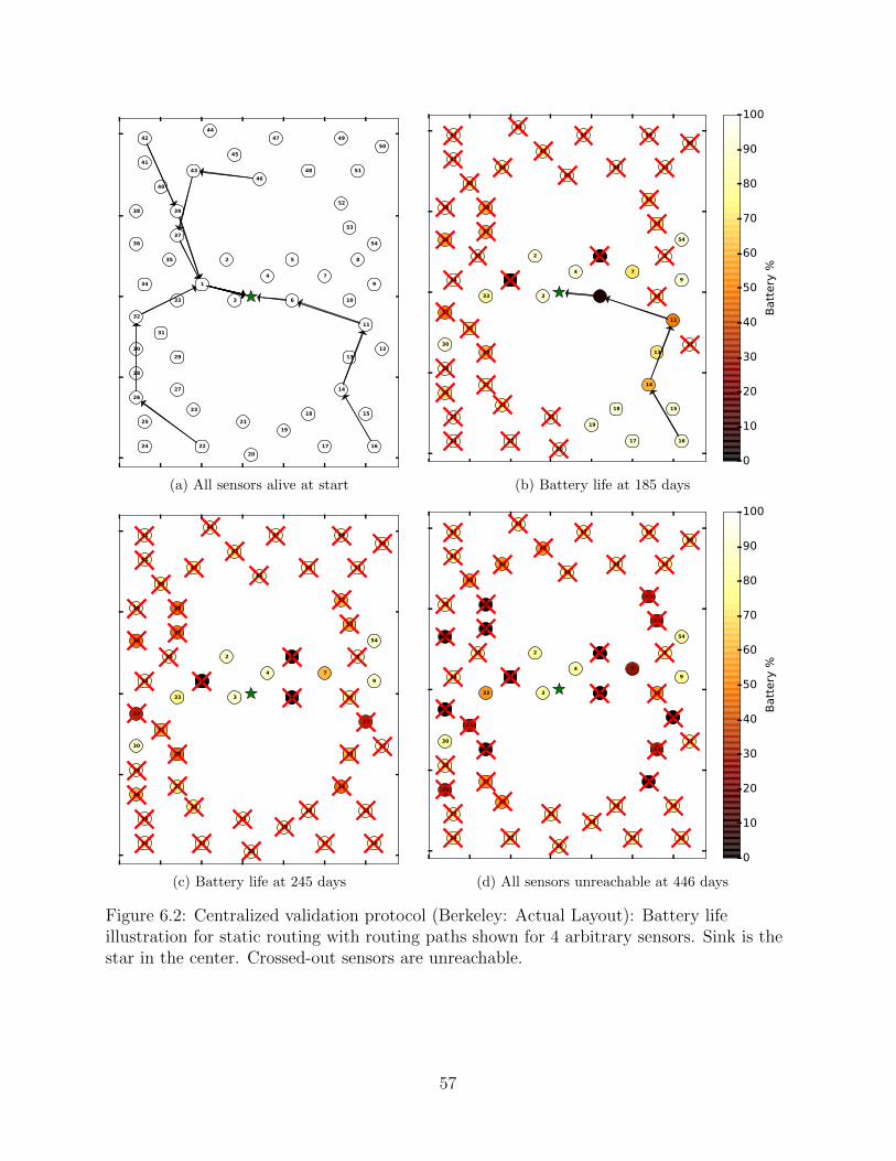
1
2
3
4
5
6
7
8
9
10
11
12
13
14
15
1617
18
19
20
21
22
23
24
25
26
27
28
29
30
31
32
33
34
35
36
37
38 39
40
41
42
43
44
45
46
47
48
49
50
51
52
53
54
(a) All sensors alive at start
1
2
3
4
5
6
7
8
9
10
11
12
13
14
15
1617
18
19
20
21
22
23
24
25
26
27
28
29
30
31
32
33
34
35
36
37
38 39
40
41
42
43
44
45
46
47
48
49
50
51
52
53
54
0
10
20
30
40
50
60
70
80
90
100
Batt
ery
%
(b) Battery life at 185 days
1
2
3
4
5
6
7
8
9
10
11
12
13
14
15
1617
18
19
20
21
22
23
24
25
26
27
28
29
30
31
32
33
34
35
36
37
38 39
40
41
42
43
44
45
46
47
48
49
50
51
52
53
54
(c) Battery life at 245 days
1
2
3
4
5
6
7
8
9
10
11
12
13
14
15
1617
18
19
20
21
22
23
24
25
26
27
28
29
30
31
32
33
34
35
36
37
38 39
40
41
42
43
44
45
46
47
48
49
50
51
52
53
54
0
10
20
30
40
50
60
70
80
90
100
Batt
ery
%
(d) All sensors unreachable at 446 days
Figure 6.2: Centralized validation protocol (Berkeley: Actual Layout): Battery lifeillustration for static routing with routing paths shown for 4 arbitrary sensors. Sink is thestar in the center. Crossed-out sensors are unreachable.
57

1
2
3
4
5
6
7
8
9
10
11
12
13
14
15
1617
18
19
20
21
22
23
24
25
26
27
28
29
30
31
32
33
34
35
36
37
38 39
40
41
42
43
44
45
46
47
48
49
50
51
52
53
54
(a) All sensors alive at start
1
2
3
4
5
6
7
8
9
10
11
12
13
14
15
1617
18
19
20
21
22
23
24
25
26
27
28
29
30
31
32
33
34
35
36
37
38 39
40
41
42
43
44
45
46
47
48
49
50
51
52
53
54
0
10
20
30
40
50
60
70
80
90
100
Batt
ery
%
(b) Battery life at 185 days
1
2
3
4
5
6
7
8
9
10
11
12
13
14
15
1617
18
19
20
21
22
23
24
25
26
27
28
29
30
31
32
33
34
35
36
37
38 39
40
41
42
43
44
45
46
47
48
49
50
51
52
53
54
(c) Battery life at 245 days
1
2
3
4
5
6
7
8
9
10
11
12
13
14
15
1617
18
19
20
21
22
23
24
25
26
27
28
29
30
31
32
33
34
35
36
37
38 39
40
41
42
43
44
45
46
47
48
49
50
51
52
53
54
0
10
20
30
40
50
60
70
80
90
100
Batt
ery
%
(d) All sensors unreachable at 446 days
Figure 6.3: P2P validation protocol (Berkeley: Actual Layout): Battery life illustration forstatic routing with routing paths shown for 4 arbitrary sensors. Sink is the star in thecenter. Crossed-out sensors are unreachable.
58
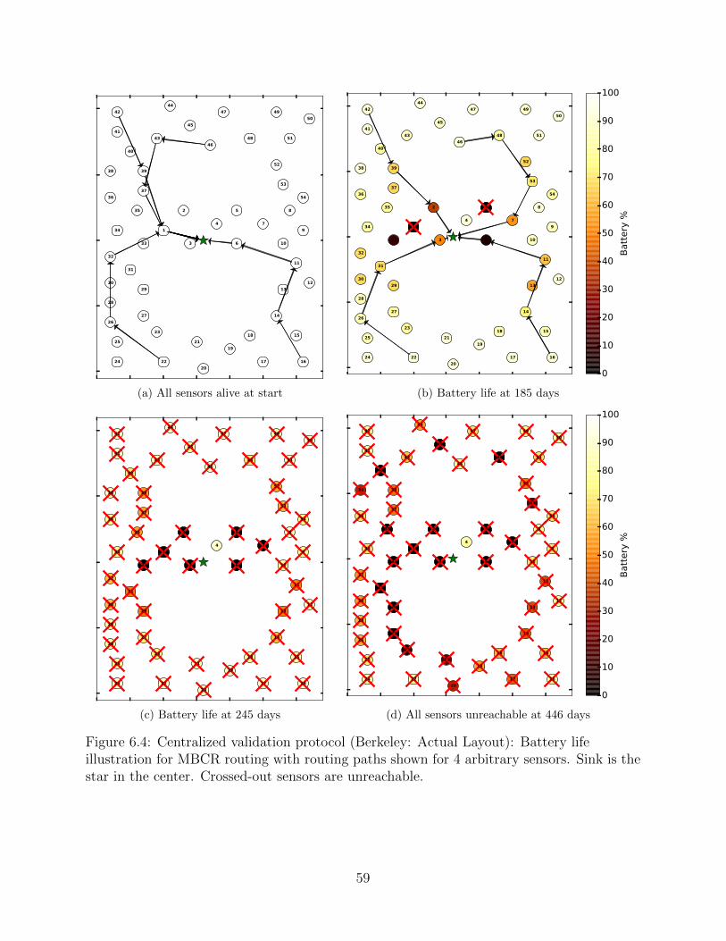
1
2
3
4
5
6
7
8
9
10
11
12
13
14
15
1617
18
19
20
21
22
23
24
25
26
27
28
29
30
31
32
33
34
35
36
37
38 39
40
41
42
43
44
45
46
47
48
49
50
51
52
53
54
(a) All sensors alive at start
1
2
3
4
5
6
7
8
9
10
11
12
13
14
15
1617
18
19
20
21
22
23
24
25
26
27
28
29
30
31
32
33
34
35
36
37
38 39
40
41
42
43
44
45
46
47
48
49
50
51
52
53
54
0
10
20
30
40
50
60
70
80
90
100
Batt
ery
%
(b) Battery life at 185 days
1
2
3
4
5
6
7
8
9
10
11
12
13
14
15
1617
18
19
20
21
22
23
24
25
26
27
28
29
30
31
32
33
34
35
36
37
38 39
40
41
42
43
44
45
46
47
48
49
50
51
52
53
54
(c) Battery life at 245 days
1
2
3
4
5
6
7
8
9
10
11
12
13
14
15
1617
18
19
20
21
22
23
24
25
26
27
28
29
30
31
32
33
34
35
36
37
38 39
40
41
42
43
44
45
46
47
48
49
50
51
52
53
54
0
10
20
30
40
50
60
70
80
90
100
Batt
ery
%
(d) All sensors unreachable at 446 days
Figure 6.4: Centralized validation protocol (Berkeley: Actual Layout): Battery lifeillustration for MBCR routing with routing paths shown for 4 arbitrary sensors. Sink is thestar in the center. Crossed-out sensors are unreachable.
59
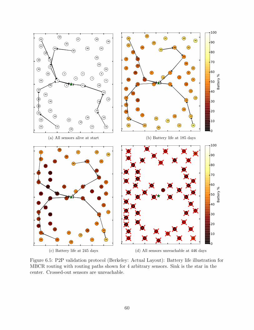
1
2
3
4
5
6
7
8
9
10
11
12
13
14
15
1617
18
19
20
21
22
23
24
25
26
27
28
29
30
31
32
33
34
35
36
37
38 39
40
41
42
43
44
45
46
47
48
49
50
51
52
53
54
(a) All sensors alive at start
1
2
3
4
5
6
7
8
9
10
11
12
13
14
15
1617
18
19
20
21
22
23
24
25
26
27
28
29
30
31
32
33
34
35
36
37
38 39
40
41
42
43
44
45
46
47
48
49
50
51
52
53
54
0
10
20
30
40
50
60
70
80
90
100
Batt
ery
%
(b) Battery life at 185 days
1
2
3
4
5
6
7
8
9
10
11
12
13
14
15
1617
18
19
20
21
22
23
24
25
26
27
28
29
30
31
32
33
34
35
36
37
38 39
40
41
42
43
44
45
46
47
48
49
50
51
52
53
54
(c) Battery life at 245 days
1
2
3
4
5
6
7
8
9
10
11
12
13
14
15
1617
18
19
20
21
22
23
24
25
26
27
28
29
30
31
32
33
34
35
36
37
38 39
40
41
42
43
44
45
46
47
48
49
50
51
52
53
54
0
10
20
30
40
50
60
70
80
90
100
Batt
ery
%
(d) All sensors unreachable at 446 days
Figure 6.5: P2P validation protocol (Berkeley: Actual Layout): Battery life illustration forMBCR routing with routing paths shown for 4 arbitrary sensors. Sink is the star in thecenter. Crossed-out sensors are unreachable.
60
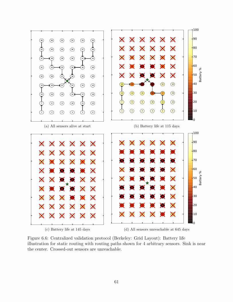
1 2 3 4 5 6
7 8 9 10 11 12
13 14 15 16 17 18
19 20 21 22 23 24
25 26 27 28 29 30
31 32 33 34 35 36
37 38 39 40 41 42
43 44 45 46 47 48
49 50 51 52 53 54
(a) All sensors alive at start
1 2 3 4 5 6
7 8 9 10 11 12
13 14 15 16 17 18
19 20 21 22 23 24
25 26 27 28 29 30
31 32 33 34 35 36
37 38 39 40 41 42
43 44 45 46 47 48
49 50 51 52 53 54
0
10
20
30
40
50
60
70
80
90
100
Batt
ery
%
(b) Battery life at 115 days
1 2 3 4 5 6
7 8 9 10 11 12
13 14 15 16 17 18
19 20 21 22 23 24
25 26 27 28 29 30
31 32 33 34 35 36
37 38 39 40 41 42
43 44 45 46 47 48
49 50 51 52 53 54
(c) Battery life at 145 days
1 2 3 4 5 6
7 8 9 10 11 12
13 14 15 16 17 18
19 20 21 22 23 24
25 26 27 28 29 30
31 32 33 34 35 36
37 38 39 40 41 42
43 44 45 46 47 48
49 50 51 52 53 54
0
10
20
30
40
50
60
70
80
90
100
Batt
ery
%
(d) All sensors unreachable at 645 days
Figure 6.6: Centralized validation protocol (Berkeley: Grid Layout): Battery lifeillustration for static routing with routing paths shown for 4 arbitrary sensors. Sink is nearthe center. Crossed-out sensors are unreachable.
61

1 2 3 4 5 6
7 8 9 10 11 12
13 14 15 16 17 18
19 20 21 22 23 24
25 26 27 28 29 30
31 32 33 34 35 36
37 38 39 40 41 42
43 44 45 46 47 48
49 50 51 52 53 54
(a) All sensors alive at start
1 2 3 4 5 6
7 8 9 10 11 12
13 14 15 16 17 18
19 20 21 22 23 24
25 26 27 28 29 30
31 32 33 34 35 36
37 38 39 40 41 42
43 44 45 46 47 48
49 50 51 52 53 54
0
10
20
30
40
50
60
70
80
90
100
Batt
ery
%
(b) Battery life at 638 days
1 2 3 4 5 6
7 8 9 10 11 12
13 14 15 16 17 18
19 20 21 22 23 24
25 26 27 28 29 30
31 32 33 34 35 36
37 38 39 40 41 42
43 44 45 46 47 48
49 50 51 52 53 54
(c) Battery life at 643 days
1 2 3 4 5 6
7 8 9 10 11 12
13 14 15 16 17 18
19 20 21 22 23 24
25 26 27 28 29 30
31 32 33 34 35 36
37 38 39 40 41 42
43 44 45 46 47 48
49 50 51 52 53 54
0
10
20
30
40
50
60
70
80
90
100
Batt
ery
%
(d) All sensors unreachable at 645 days
Figure 6.7: P2P validation protocol (Berkeley: Grid Layout): Battery life illustration forstatic routing with routing paths shown for 4 arbitrary sensors. Sink is near the center.Crossed-out sensors are unreachable.
62
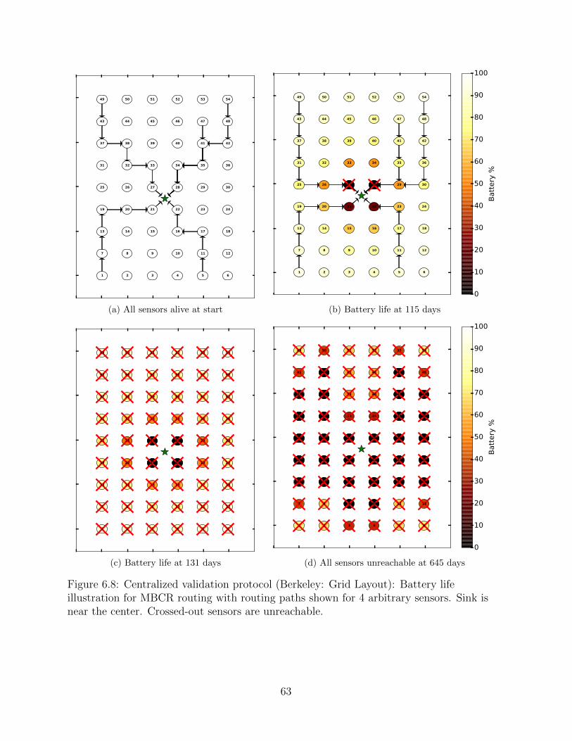
1 2 3 4 5 6
7 8 9 10 11 12
13 14 15 16 17 18
19 20 21 22 23 24
25 26 27 28 29 30
31 32 33 34 35 36
37 38 39 40 41 42
43 44 45 46 47 48
49 50 51 52 53 54
(a) All sensors alive at start
1 2 3 4 5 6
7 8 9 10 11 12
13 14 15 16 17 18
19 20 21 22 23 24
25 26 27 28 29 30
31 32 33 34 35 36
37 38 39 40 41 42
43 44 45 46 47 48
49 50 51 52 53 54
0
10
20
30
40
50
60
70
80
90
100
Batt
ery
%
(b) Battery life at 115 days
1 2 3 4 5 6
7 8 9 10 11 12
13 14 15 16 17 18
19 20 21 22 23 24
25 26 27 28 29 30
31 32 33 34 35 36
37 38 39 40 41 42
43 44 45 46 47 48
49 50 51 52 53 54
(c) Battery life at 131 days
1 2 3 4 5 6
7 8 9 10 11 12
13 14 15 16 17 18
19 20 21 22 23 24
25 26 27 28 29 30
31 32 33 34 35 36
37 38 39 40 41 42
43 44 45 46 47 48
49 50 51 52 53 54
0
10
20
30
40
50
60
70
80
90
100
Batt
ery
%
(d) All sensors unreachable at 645 days
Figure 6.8: Centralized validation protocol (Berkeley: Grid Layout): Battery lifeillustration for MBCR routing with routing paths shown for 4 arbitrary sensors. Sink isnear the center. Crossed-out sensors are unreachable.
63
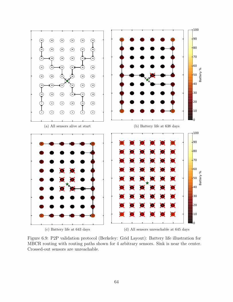
1 2 3 4 5 6
7 8 9 10 11 12
13 14 15 16 17 18
19 20 21 22 23 24
25 26 27 28 29 30
31 32 33 34 35 36
37 38 39 40 41 42
43 44 45 46 47 48
49 50 51 52 53 54
(a) All sensors alive at start
1 2 3 4 5 6
7 8 9 10 11 12
13 14 15 16 17 18
19 20 21 22 23 24
25 26 27 28 29 30
31 32 33 34 35 36
37 38 39 40 41 42
43 44 45 46 47 48
49 50 51 52 53 54
0
10
20
30
40
50
60
70
80
90
100
Batt
ery
%
(b) Battery life at 638 days
1 2 3 4 5 6
7 8 9 10 11 12
13 14 15 16 17 18
19 20 21 22 23 24
25 26 27 28 29 30
31 32 33 34 35 36
37 38 39 40 41 42
43 44 45 46 47 48
49 50 51 52 53 54
(c) Battery life at 643 days
1 2 3 4 5 6
7 8 9 10 11 12
13 14 15 16 17 18
19 20 21 22 23 24
25 26 27 28 29 30
31 32 33 34 35 36
37 38 39 40 41 42
43 44 45 46 47 48
49 50 51 52 53 54
0
10
20
30
40
50
60
70
80
90
100
Batt
ery
%
(d) All sensors unreachable at 645 days
Figure 6.9: P2P validation protocol (Berkeley: Grid Layout): Battery life illustration forMBCR routing with routing paths shown for 4 arbitrary sensors. Sink is near the center.Crossed-out sensors are unreachable.
64

6.2.5 NZ: Actual Layout
For the NZ dataset, we consider five sensors spaced around Mount Ruapehu (which is an
active volcano in New Zealand) in a ring topology. We do not consider the remaining
sensors in the dataset because they are spread out hundreds of miles apart, and located in
different regional networks. The sink could not be placed in the center of the ring (inside
the volcano), so it was placed in the ring, within range of two of the sensors (which achieves
better reachability than having it within range of only one sensor, which would be a routing
bottleneck). Snapshots for static routing in both protocols are illustrated in Fig. 6.10 and
Fig. 6.11. On Day 629, 3 sensors had just lost reachability with the centralized protocol.
That day is also clearly marked by the solid red line in Fig. 6.17.
Snapshots for MBCR routing in both protocols are illustrated in Fig. 6.12 and Fig. 6.13.
It is clear from both static and MBCR illustrations that the P2P approach dramatically
improves reachability.
65
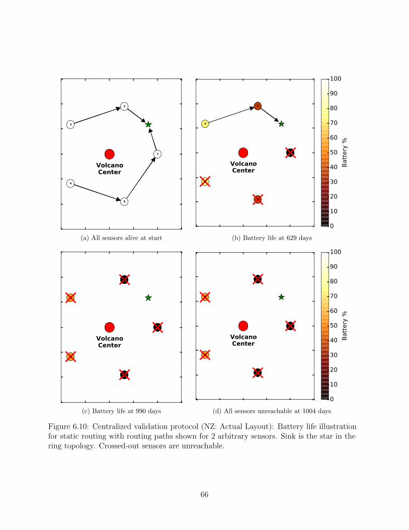
1
2
3
4
5
VolcanoCenter
(a) All sensors alive at start
1
2
3
4
5
VolcanoCenter
0
10
20
30
40
50
60
70
80
90
100
Batt
ery
%
(b) Battery life at 629 days
1
2
3
4
5
VolcanoCenter
(c) Battery life at 990 days
1
2
3
4
5
VolcanoCenter
0
10
20
30
40
50
60
70
80
90
100
Batt
ery
%
(d) All sensors unreachable at 1004 days
Figure 6.10: Centralized validation protocol (NZ: Actual Layout): Battery life illustrationfor static routing with routing paths shown for 2 arbitrary sensors. Sink is the star in thering topology. Crossed-out sensors are unreachable.
66

1
2
3
4
5
VolcanoCenter
(a) All sensors alive at start
1
2
3
4
5
VolcanoCenter
0
10
20
30
40
50
60
70
80
90
100
Batt
ery
%
(b) Battery life at 629 days
1
2
3
4
5
VolcanoCenter
(c) Battery life at 990 days
1
2
3
4
5
VolcanoCenter
0
10
20
30
40
50
60
70
80
90
100
Batt
ery
%
(d) All sensors unreachable at 1004 days
Figure 6.11: P2P validation protocol (NZ: Actual Layout): Battery life illustration forstatic routing with routing paths shown for 2 arbitrary sensors. Sink is the star in the ringtopology
67
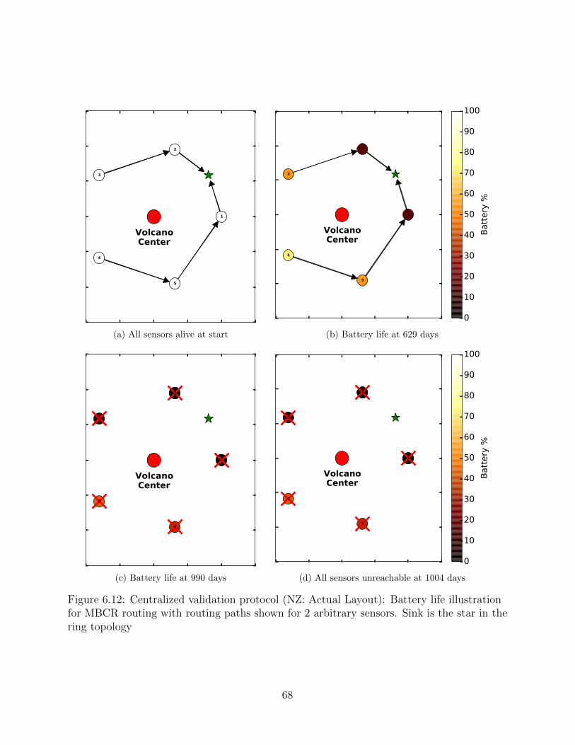
1
2
3
4
5
VolcanoCenter
(a) All sensors alive at start
1
2
3
4
5
VolcanoCenter
0
10
20
30
40
50
60
70
80
90
100
Batt
ery
%
(b) Battery life at 629 days
1
2
3
4
5
VolcanoCenter
(c) Battery life at 990 days
1
2
3
4
5
VolcanoCenter
0
10
20
30
40
50
60
70
80
90
100
Batt
ery
%
(d) All sensors unreachable at 1004 days
Figure 6.12: Centralized validation protocol (NZ: Actual Layout): Battery life illustrationfor MBCR routing with routing paths shown for 2 arbitrary sensors. Sink is the star in thering topology
68
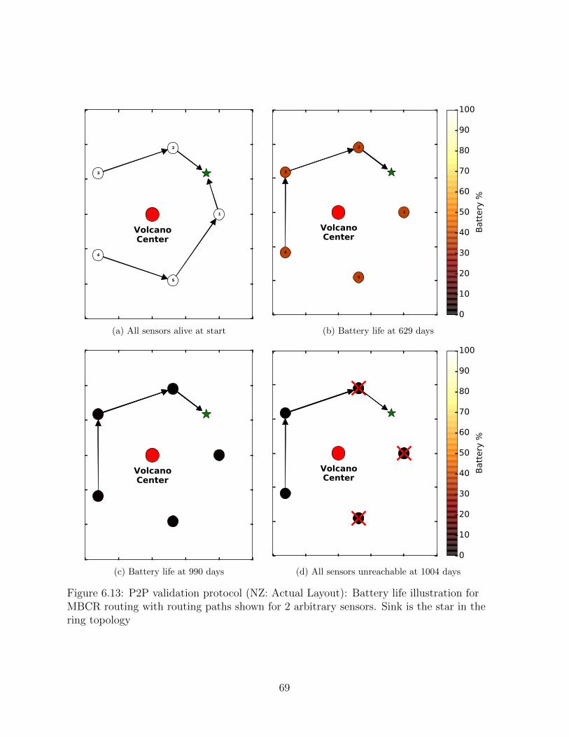
1
2
3
4
5
VolcanoCenter
(a) All sensors alive at start
1
2
3
4
5
VolcanoCenter
0
10
20
30
40
50
60
70
80
90
100
Batt
ery
%
(b) Battery life at 629 days
1
2
3
4
5
VolcanoCenter
(c) Battery life at 990 days
1
2
3
4
5
VolcanoCenter
0
10
20
30
40
50
60
70
80
90
100
Batt
ery
%
(d) All sensors unreachable at 1004 days
Figure 6.13: P2P validation protocol (NZ: Actual Layout): Battery life illustration forMBCR routing with routing paths shown for 2 arbitrary sensors. Sink is the star in thering topology
69

6.3 Detection Accuracy Results
In terms of error detection accuracy, both the centralized and P2P algorithms performed
equally well on all datasets, consistently identifying the faulty sensors and reporting zero false
positives at an isocontour threshold of k = 3. For the NZ dataset, that threshold successfully
reported anomalies due to faults as well as abnormal seismic activity. We manually inspected
potential false positives and noticed that there were indeed deviations in the data when errors
were reported.
6.4 Reachability Results
We designed experiments on our simulator that illustrate the impact of the P2P and central-
ized validation protocols on sensor network longevity and reachability. We evaluated both
protocols on three different datasets having different sensor layouts. In general, the results
show that reachability is maximized with our P2P protocol using MBCR routing. The P2P
protocol also improves longevity up until sensors get disconnected. Once sensors are discon-
nected, the centralized protocol provides better longevity due to less CPU drain. However
that advantage of the centralized protocol is irrelevant because the sensors are effectively
dead from the sink’s perspective once they are disconnected.
6.4.1 Notation for Metrics
We describe our evaluation metrics, stated in Section 2, formally in this subsection.
Let Λ(t) = λ be the number of sensors that are dead (due to battery depletion) at time t.
Then Longevity(λ) = mint : Λ(t) = λ. In other words, longevity can be described as
the inverse function of Λ(t). However, illustrating Λ(t) is more intuitive because functions
of time are more commonly illustrated. Therefore, we illustrate Λ(t) instead.
Let Ω(t) = ω be the number of sensors that have lost end-to-end connectivity with the
sink (in other words, become unreachable) at time t.
Then Reachability(ω) = mint : Ω(t) = ω. In other words, reachability can be described
70

as the inverse function of Ω(t). However, illustrating Ω(t) is more intuitive for the same
reasons as it was for Λ(t).
The system should ideally have both high Longevity and high Reachability. That is
because we want the sensors to last longer and be reachable for longer periods of time.
6.4.2 Berkeley Dataset (Actual Layout)
Figure 6.14(a) is in agreement with Figs. 6.4 and 6.5. As shown in Fig. 6.14(a), the P2P
approach improves reachability for all of the sensors in MBCR and 85% of the sensors
in static routing. The remaining few sensors that survived in static routing were on few
or zero multi-hop routes to begin with because of their location in the lab. Thus, their
communication overhead was the same in both protocols, and the computation overhead
high in P2P.
For 50% of the sensors in static routing, the P2P protocol improved reachability by over
4× that of the centralized protocol. Those sensors became unreachable when the root nodes
they forwarded through died. MBCR improved their reachability because it dynamically
found a new route to maintain connectivity with the sink. Therefore, our P2P protocol had
lesser of an advantage over the centralized protocol with MBCR routing.
6.4.3 Berkeley Dataset (Grid Layout)
It is clear from Fig. 6.15 that the P2P approach improves reachability by three to four times.
The MBCR routing protocol provides negligible improvement over static routing in reacha-
bility of the network as a whole, not favoring any specific sensors for greater reachability.
71

0 500 1000 1500 2000 2500Time (Days): t
0
10
20
30
40
50
60
Num
ber
of
Dead S
enso
rs: Λ
(t)
Centralized Static
Centralized MBCR
P2P Static
P2P MBCR
(a) Longevity
0 200 400 600 800 1000Time (Days): t
0
10
20
30
40
50
60
Num
ber
of
Unre
ach
able
Senso
rs: Ω
(t)
Centralized Static
Centralized MBCR
P2P Static
P2P MBCR
(b) Reachability
Figure 6.14: Results for Intel Berkeley Dataset (Actual Layout). The inverse functions ofLongevity and Reachability, which are the number of sensors dead and unreachable,respectively, are plotted.
72

0 500 1000 1500 2000 2500Time (Days): t
0
10
20
30
40
50
60
Num
ber
of
Dead S
enso
rs: Λ
(t)
Centralized Static
Centralized MBCR
P2P Static
P2P MBCR
(a) Longevity
0 200 400 600 800 1000 1200 1400 1600Time (Days): t
0
10
20
30
40
50
60
Num
ber
of
Unre
ach
able
Senso
rs: Ω
(t)
Centralized Static
Centralized MBCR
P2P Static
P2P MBCR
(b) Reachability
Figure 6.15: Results for Intel Berkeley Dataset (Grid Layout). The inverse functions ofLongevity and Reachability, which are the number of sensors dead and unreachable,respectively, are plotted.
73

6.4.4 TAO Dataset Experiments
In this layout, all 8 sensors were placed in a linear physical topology to resemble their actual
placement on the equator. The sink was placed at one end. The P2P protocol improved
reachability by 4.5× over the centralized protocol for both static and MBCR routing, as
shown in Fig. 6.16.
6.4.5 NZ Dataset Experiments
The P2P protocol improved reachability by 60% and 30% over the centralized protocol
for static and MBCR routing, respectively for 60% of sensors, as illustrated in Fig. 6.17.
The P2P protocol performed equally well with static and MBCR routing because of a lack
of routing options in the limited topology (reachability was extended by MBCR by only
two days, and the overlapping curves are not shown separately in the figure to improve
readability).
74

0 500 1000 1500 2000 2500Time (Days): t
0
1
2
3
4
5
6
7
8
9
Num
ber
of
Dead S
enso
rs: Λ
(t)
Centralized Static
Centralized MBCR
P2P Static
P2P MBCR
(a) Longevity
0 500 1000 1500 2000Time (Days): t
0
1
2
3
4
5
6
7
8
Num
ber
of
Unre
ach
able
Senso
rs: Ω
(t)
Centralized Static
Centralized MBCR
P2P Static
P2P MBCR
(b) Reachability
Figure 6.16: Results for TAO Dataset. The inverse functions of Longevity and Reachability,which are the number of sensors dead and unreachable, respectively, are plotted.
75

0 500 1000 1500 2000 2500Time (Days): t
0.0
0.5
1.0
1.5
2.0
2.5
3.0
3.5
4.0
Num
ber
of
Dead S
enso
rs: Λ
(t)
Centralized Static
Centralized MBCR
P2P Static
P2P MBCR
(a) Longevity
0 500 1000 1500 2000Time (Days): t
0
1
2
3
4
5
Num
ber
of
Unre
ach
able
Senso
rs: Ω
(t)
Centralized Static
Centralized MBCR
P2P Static/MBCR
(b) Reachability
Figure 6.17: Results for NZ Dataset. The inverse functions of Longevity and Reachability,which are the number of sensors dead and unreachable, respectively, are plotted.
76

CHAPTER 7
RELATED WORK
There is an extensive literature on the design of anomaly detection protocols (surveyed
in [27]), and on energy-efficient protocols for WSNs (surveyed in [9]). The literatures on
those two topics are largely separate, despite the need for an integrated solution. The topics
have separately received attention from the dependable systems and networks community [7,
13,14,17,19], as cited throughout the thesis.
Elnahrawy and Nath [28] leverage contextual information in the form of spatial correlations
to detect anomalies, similar to our approach. However, they fail to address the impact of
adding validation features on sensor battery and WSN survivability.
Paola et al. [29], propose an adaptive distributed outlier detector algorithm to detect
faults in WSNs. The algorithm overlays a Bayesian network on the network topology that
propagates belief in the sensor’s correctness. The limitation of that approach is that con-
ditional probabilities on the hidden variables in the Bayesian network need to be computed
for each sensor offline using supervised learning. In contrast, our approach is completely
unsupervised, significantly simplifying its installation and set-up.
Dua et al. [30] rely on a hardware-based trusted platform module (TPM) on each sensor
to enable trust by attesting to the integrity of the data. We do not require an expensive
TPM approach because we assume that a sensor may report false data, but not maliciously
or in collusion with others.
Meng et al. [11] present two techniques to ascertain the true value reported by multiple,
possibly unreliable sensors by leveraging the correlation among different sensors. In their
system, the sensors act as clients and submit their information to a centralized server. The
server solves an optimization problem to detect anomalies. Our method takes a different
approach and allows each sensor to act locally as a measurement validator to minimize the
77

overhead of routing packets through the WSN to a centralized server.
Rajasegarar et al. [31] propose an in-network anomaly detector that uses a cluster-based
approach for energy efficiency. However, the way the authors measure dissimilarity and
form clusters differs from our approach. The authors use Euclidean distances as a way to
measure dissimilarity and use a fixed-width clustering algorithm, while we use regression
based techniques to measure dissimilarity.
Branch et al. [32] also demonstrate an in-network anomaly detection approach, but they
make the assumption that every sensor in the network has to be made aware of the anomaly.
We relax that assumption in our model and require that a quorum of validating sensors in
a group be aware of the anomalous sensor in that group. This results in reduced message
transmission in the power-constrained network, yet it effectively and efficiently serves the
purpose of identifying the faulty sensor.
A patent by Samsung [33] proposes a scheme in which an aggregator collects information
from a number of sensors and informs the base station (sink). A base station selects one or
more verifiers and commands the aggregator to submit the information to the verifiers for
verification. The verifiers choose a random subset of the sensors and query them to determine
whether the aggregator’s result is truthful. This differs from our approach, in which every
sensor could in theory act as a validator with no explicit coordination or command from an
aggregator or base station.
Sundaram and Eugster [17] provide a lightweight tracing mechanism for debugging sensor
networks when messages are lost, dropped or received out of order. We do not consider such
errors, and instead focus on measurement errors.
Zhang and Liu [34] present DataGuard, a software-based approach to protect the integrity
of the memory and software running on the sensors from attacks. Unlike our work, that
approach is not concerned with detecting non-malicious measurement errors.
Khalil et al. [13] present SLAM, a method to monitor neighboring sensors for suspicious
behavior using a Sleep-Wake protocol that extends battery life. While our approach can
use similar sleep-wake methods, we monitor sensors for erroneous measurements, and not
suspicious behavior.
Basile et al. [19] provide a method that uses Hidden Markov Models to characterize anoma-
78

lies as caused by malicious or non-malicious faults. That method can be used in conjunction
with our work, if a network administrator desired to make that differentiation.
Liu et al. [7] describe the detection of erroneous measurements in structural health moni-
toring applications. They do no consider the impact of their methods on sensor battery life,
and their approaches may dramatically benefit from our work.
79

CHAPTER 8
CONCLUSION
In this thesis, we developed a P2P protocol that detects erroneous measurements in a WSN
while simultaneously minimizing the impact of the detection overhead on its reachability.
Using a simulation tool built to evaluate the protocol, we confirmed our hypothesis that
sensor networks that employ the naive centralized error detection approach will drain sensors
near the sink, disconnecting sensors farther away from it. In contrast, the P2P approach is
less harsh on the sensors near the sink. The P2P protocol trades off computation savings for
communication savings; it moves the onus of error detection from the sink onto the sensors
themselves, and in doing so, it minimizes the number of messages required to report an error.
Since communication consumes more energy on a sensor than computation, that trade-off
effectively allows sensors to remain connected to the sink for a significantly longer period of
time.
In our distributed protocol, anomalous data from erroneous sensors were flagged by the
sensors themselves and reported to the sink. In future work, we may explore a self-healing
approach in which sensors report anomalies to a validators in the network that are nearer
to them than the sink. A validator would command an erroneous sensor to stop measuring
and reporting data. That would obviate the need to report to the sink, saving even more
energy. However, the sink would lose some knowledge of what is happening in the network
and therein lies a trade-off.
80
APPENDIX A
UNSUITABLE ANOMALY DETECTIONAPPROACHES
In this appendix we describe anomaly detection approaches that were considered, but not
adopted because of their unsuitability for the purpose of validating sensor measurements.
A.1 OLS Linear Regression
Our first thought was to use ordinary least squares (OLS) linear regression because we
observed that sensor values tended to be linearly related, as seen in Fig. 3.3, in all our
datasets.
Consider two sensors S(1) and S(19) whose measurements at time t, S(1)t and S
(19)t , are
linearly related as follows:
S(19)t = mS
(1)t + c+ ε (A.1)
The variables m and c are scalars representing the slope and intercept of the linear re-
lationship, and the residual ε ∼ N(0, σ2) represents Gaussian white noise in the relative
measurements. Given this Gaussian assumption, which is also made in [10], OLS linear
regression is solved by minimizing the L2-norm of the residuals (which is itself a vector of ε
values obtained from T latest sensor measurements). Since T is not large, the closed-form
solution for linear regression can be computed without having to resort to CPU-intensive
gradient descent methods.
Consider the scenario in which sensor S(19) validates its measurements with respect to
another sensor S(1) with which it is linearly related. S(19) does so by building a model of
S(1)’s measurements using linear regression and storing the model parameters m, c, and σ.
Those model parameters are estimated using the latest T measurements of S(1), which were
81

6000 4000 2000 0 2000 4000 6000 8000Sensor 19 Measurements
100000
80000
60000
40000
20000
0
20000
40000Senso
r 1 M
easu
rem
ents
Scatter Plot and TLS Fitting
OLS Fitting Line
Normal Points
Anomalous Point
30000 20000 10000 0 10000 20000 30000Sensor 1 Errors
0.00000
0.00001
0.00002
0.00003
0.00004
0.00005
0.00006
Pro
babili
ty D
ensi
ty
Projection Errors
Figure A.1: NZ dataset: OLS regression used in anomaly detection.
stored in S(19)’s memory. At time t, S(19) computes the residual εt = S(2)t − (mS(1) + c) and
compares this to a threshold. This is illustrated in Fig. A.1, where the past residuals (or
fitting errors) of S(1) clearly form a Gaussian distribution.
There are many ways to choose a threshold for anomaly detection, and the choice de-
termines the detection (true positive) and false positive rate. We adopt the common 3σ
threshold, where ε ∼ N(0, σ2). If the observed residual |εt| > 3σ, then the probability that
S(2)t is valid given S
(1)t is P (|εt| > 3σ) = 0.3%, so S
(2)t will be flagged as anomalous.
The similarity metric is used by each sensor in our protocol to decide which other sensors
should be its reference sensors for the purposes of anomaly detection. If S(1) and S(2) are
perfectly collinear, then εt = S(2)t − (mS
(1)t + c) = 0. If they are highly collinear, then
|εt| = |S(2)t − (mS
(1)t + c)| approaches zero. This implies that σ must also approach zero,
since ε ∼ N(0, σ2) can be written as ε = σz, where z ∼ N(0, 1). As a result, high collinearity
implies a smaller σ (sensor measurements are very similar), and low collinearity implies a
larger σ (sensor measurements are dissimilar). Therefore, collinearity is a suitable similarity
metric.
The failure of this method lies in its asymmetry. Symmetry was an essential property
of the algorithm for our protocol, as described in Section 4.5. Figure A.2 shows that even
82

100000 80000 60000 40000 20000 0 20000 40000Sensor 1 Measurements
6000
4000
2000
0
2000
4000
6000
8000Senso
r 19 M
easu
rem
ents
Scatter Plot and TLS Fitting
OLS Fitting Line
Normal Points
Anomalous Point
6000 4000 2000 0 2000 4000 6000Sensor 19 Errors
0.00000
0.00005
0.00010
0.00015
0.00020
0.00025
Pro
babili
ty D
ensi
ty
Projection Errors
Figure A.2: NZ dataset: Failure of OLS regression used in anomaly detection.
though the measurement taken by Sensor 1 appears anomalous with respect to Sensor 19, the
reverse does not hold. The measurement taken by Sensor 19 is not anomalous with respect
to Sensor 1 because of the manner in which the fitting line is drawn by OLS regression. The
line is drawn to minimize the vertical distance (parallel to the vertical axis) between points
and the line.
A.2 TLS Linear Regression
Total least squares (TLS) linear regression or orthogonal regression provides a symmetric
approach to finding a fitting line by finding a line that minimizes the orthogonal distance
between the points and the line.
In order to estimate the line, we can use the Eckart-Young theorem to relate the mini-
mization of the Frobenius norm of the projection errors with the principal components of
the measurement data. We omit the details here, but it can be proven that this method is
symmetric in the fitting line it produces. The projection errors of the original data points
on the fitting line are Gaussian, as shown in Fig. A.3.
83

100000 80000 60000 40000 20000 0 20000 40000Sensor 1 Measurements
60000
40000
20000
0
20000
40000
60000
Senso
r 19 M
easu
rem
ents
Scatter Plot and TLS Fitting
TLS Fitting Line
Normal Points
Anomalous Point
80 60 40 20 0 20 40 60 80Sensor 1 Errors
0.000
0.002
0.004
0.006
0.008
0.010
0.012
0.014
Pro
babili
ty D
ensi
ty
6000 4000 2000 0 2000 4000 6000Sensor 19 Errors
0.00000
0.00005
0.00010
0.00015
0.00020
0.00025
Pro
babili
ty D
ensi
ty
(a) Sensor 19 with respect to Sensor 1
60000 40000 20000 0 20000 40000 60000Sensor 19 Measurements
100000
80000
60000
40000
20000
0
20000
40000
Senso
r 1 M
easu
rem
ents
Scatter Plot and TLS Fitting
TLS Fitting Line
Normal Points
Anomalous Point
6000 4000 2000 0 2000 4000 6000Sensor 19 Errors
0.00000
0.00005
0.00010
0.00015
0.00020
0.00025
Pro
babili
ty D
ensi
ty
80 60 40 20 0 20 40 60 80Sensor 1 Errors
0.000
0.002
0.004
0.006
0.008
0.010
0.012
0.014
Pro
babili
ty D
ensi
ty
(b) Sensor 1 with respect to Sensor 19
Figure A.3: NZ dataset: TLS regression used in anomaly detection.
84

Although this approach provides symmetry, unlike OLS regression, it is not suitable for
anomaly detection. As can be seen in Fig. A.3, the anomalous point lies almost on the best
fit line. Therefore, the approach does not detect the anomaly.
A good approach would not look for anomalies in only one dimension because that could
miss the anomaly in the orthogonal dimension. Therefore we choose to use a two-dimensional
approach leveraging bivariate Gaussian isocontours.
A.3 Correlation and Dot Products
Correlation and dot products have been suggested in related work [27] for anomaly detec-
tion. We believe that these are reasonable similarity metrics, but impractical for anomaly
detection. Both correlation and dot products apply to vectors. Assume that we have T
points of historic data from two sensors. That can produce one value for the correlation or
the dot product. With that one value it is difficult to tell whether a new pair of points from
the two sensors is anomalous or not. One would need to calculate the change that the new
value causes to the correlation or dot product, assuming that those values do not tend to
change much (to the best of our knowledge, there is no well-known underlying probabilistic
behavior associated with that change). In our approach, however, there is a clear decision
boundary constructed from a bivariate normal distribution, which captures the tendency of
the data to cluster together.
85

APPENDIX B
SENSOR ID AND NAME MAPPING
B.1 Berkeley Dataset
The sensors were numbered as given in the layout in [2].
B.2 TAO Dataset
0 - sst0n110w
1 - sst0n125w
2 - sst0n140w
3 - sst0n155w
4 - sst0n165e
5 - sst0n170w
6 - sst0n180w
7 - sst0n95w
B.3 NZ Dataset
0 - APZ.HHZ.10.NZ
1 - BFZ.HHZ.10.NZ
2 - BKZ.HHZ.10.NZ
3 - COVZ.HHZ.10.NZ
4 - CTZ.HHZ.10.NZ
86

5 - CVZ.HHZ.10.NZ
6 - DCZ.HHZ.10.NZ
7 - DSZ.HHZ.10.NZ
8 - EAZ.HHZ.10.NZ
9 - ETVZ.HHZ.10.NZ
10 - FOZ.HHZ.10.NZ
11 - FWVZ.HHZ.10.NZ
12 - GLKZ.HHZ.10.NZ
13 - GRZ.HHZ.10.NZ
14 - GVZ.HHZ.10.NZ
15 - HAZ.HHZ.10.NZ
16 - MAVZ.HHZ.10.NZ
17 - MLZ.HHZ.10.NZ
18 - MQZ.HHZ.10.NZ
19 - MRZ.HHZ.10.NZ
20 - MSZ.HHZ.10.NZ
21 - MWZ.HHZ.10.NZ
22 - MXZ.HHZ.10.NZ
23 - PUZ.HHZ.10.NZ
24 - PXZ.HHZ.10.NZ
25 - PYZ.HHZ.10.NZ
26 - THZ.HHZ.10.NZ
27 - TLZ.HHZ.10.NZ
28 - TMVZ.HHZ.10.NZ
29 - TOZ.HHZ.10.NZ
30 - TRVZ.HHZ.10.NZ
31 - TSZ.HHZ.10.NZ
32 - TUZ.HHZ.10.NZ
33 - WCZ.HHZ.10.NZ
34 - WEL.HHZ.10.NZ
87

35 - WHVZ.HHZ.10.NZ
36 - WHZ.HHZ.10.NZ
37 - WIZ.HHZ.10.NZ
38 - WKZ.HHZ.10.NZ
39 - WSRZ.HHZ.10.NZ
40 - WVZ.HHZ.10.NZ
88

REFERENCES
[1] GeoNet Project, “GeoNet National Seismograph Network dataset,” Date LastAccessed: 6 Nov 2016. [Online]. Available: http://doi.org/10.21420/G2WC7M
[2] S. Madden, “Intel lab data,” 2004, Date Last Accessed: 6 Nov 2016. [Online].Available: http://db.csail.mit.edu/labdata/labdata.html
[3] G. Tolle, J. Polastre, R. Szewczyk, D. Culler, N. Turner, K. Tu, S. Burgess, T. Daw-son, P. Buonadonna, D. Gay, and W. Hong, “A macroscope in the redwoods,” in InProceedings SenSys ’05. New York, NY, USA: ACM, 2005, pp. 51–63.
[4] R. Szewczyk, A. Mainwaring, J. Polastre, J. Anderson, and D. Culler, “An analysis of alarge scale habitat monitoring application,” in Proceedings of SenSys ’04. New York,NY, USA: ACM, 2004, pp. 214–226.
[5] J. Burrell, T. Brooke, and R. Beckwith, “Vineyard computing: sensor networks inagricultural production,” IEEE Pervasive Computing, vol. 3, no. 1, pp. 38–45, Jan2004.
[6] G. Werner-Allen, K. Lorincz, J. Johnson, J. Lees, and M. Welsh, “Fidelity and yield in avolcano monitoring sensor network,” in Proceedings of OSDI ’06. USENIX Association,2006, pp. 381–396.
[7] X. Liu, J. Cao, M. Bhuiyan, S. Lai, H. Wu, and G. Wang, “Fault tolerant wsn-basedstructural health monitoring,” in 2011 IEEE/IFIP 41st International Conference onDependable Systems Networks (DSN), June 2011, pp. 37–48.
[8] S. Kim, S. Pakzad, D. Culler, J. Demmel, G. Fenves, S. Glaser, and M. Turon, “Healthmonitoring of civil infrastructures using wireless sensor networks,” in Proceedings ofIPSN ’07, April 2007, pp. 254–263.
[9] G. M. Shafiullah, A. Gyasi-Agyei, and P. J. Wolfs, “A survey of energy-efficient andqos-aware routing protocols for wireless sensor networks,” in Novel Algorithms andTechniques In Telecommunications, Automation and Industrial Electronics, T. Sobh,K. Elleithy, A. Mahmood, and M. A. Karim, Eds. Dordrecht: Springer Netherlands,2008, pp. 352–357.
89

[10] S. Alag, A. M. Agogino, and M. Morjaria, “A methodology for intelligent sensor mea-surement, validation, fusion, and fault detection for equipment monitoring and diag-nostics,” Artificial Intelligence for Engineering Design, Analysis and Manufacturing,vol. 15, no. 4, pp. 307–320, Sep. 2001.
[11] C. Meng, W. Jiang, Y. Li, J. Gao, L. Su, H. Ding, and Y. Cheng, “Truth discovery oncrowd sensing of correlated entities,” in Proceedings of SenSys ’15. New York, NY,USA: ACM, 2015, pp. 169–182.
[12] S. Madden, M. J. Franklin, J. M. Hellerstein, and W. Hong, “TAG: A Tiny AGgregationService for ad-hoc sensor networks,” SIGOPS Oper. Syst. Rev., vol. 36, no. SI, pp. 131–146, Dec. 2002.
[13] I. Khalil, S. Bagchi, and N. B. Shroff, “Slam: Sleep-wake aware local monitoring insensor networks,” in 37th Annual IEEE/IFIP International Conference on DependableSystems and Networks (DSN’07), June 2007, pp. 565–574.
[14] G. Khanna, S. Bagchi, and Y.-S. Wu, “Fault tolerant energy aware data disseminationprotocol in sensor networks,” in Proc. of DSN, June 2004.
[15] C. K. Toh, H. Cobb, and D. A. Scott, “Performance evaluation of battery-life-awarerouting schemes for wireless ad hoc networks,” in Proceedings of ICC ’01, vol. 9, 2001,pp. 2824–2829 vol.9.
[16] A. Das, I. Gupta, and A. Motivala, “Swim: scalable weakly-consistent infection-styleprocess group membership protocol,” in Proceedings of DSN, 2002, pp. 303–312.
[17] V. Sundaram and P. Eugster, “Lightweight message tracing for debugging wireless sen-sor networks,” in 2013 43rd Annual IEEE/IFIP International Conference on DependableSystems and Networks (DSN), June 2013, pp. 1–12.
[18] L. Paradis and Q. Han, “Tigra: Timely sensor data collection using distributed graphcoloring,” in Proceedings of PerCom ’08, March 2008, pp. 264–268.
[19] C. Basile, M. Gupta, Z. Kalbarczyk, and R. K. Iyer, “An approach for detecting anddistinguishing errors versus attacks in sensor networks,” in International Conference onDependable Systems and Networks (DSN’06), June 2006, pp. 473–484.
[20] Pacific Marine Environmental Laboratory, “Tropical Atmosphere Ocean Project,”Date Last Accessed: 6 Nov 2016. [Online]. Available: http://www.pmel.noaa.gov/tao/proj over/mooring.shtml
[21] V. Badrinath Krishna, R. K. Iyer, and W. H. Sanders, “ARIMA-Based Modeling andValidation of Consumption Readings in Power Grids,” in Proceedings of Critical Infor-mation Infrastructure Security (CRITIS). Springer Verlag, 2015.
[22] F. Yu, “A survey of wireless sensor network simulation tools,” April 2011. [Online].Available: http://www.cse.wustl.edu/∼jain/cse567-11/ftp/sensor/index.html
90

[23] Information Sciences Institute, “The network simulator - NS-2,” January 2016.[Online]. Available: http://www.isi.edu/nsnam/ns/
[24] P. Levis and N. Lee, “TOSSIM: A simulator for TinyOS networks,” June 2003.[Online]. Available: http://www.tinyos.net/tinyos-1.x/doc/nido.pdf
[25] “Mica2dot wireless microsensor mote,” Date Last Accessed: 6 Dec 2016. [Online].Available: https://www.eol.ucar.edu/isf/facilities/isa/internal/CrossBow/DataSheets/mica2dot.pdf
[26] F. Ferrari, M. Zimmerling, L. Mottola, and L. Thiele, “Low-power wireless bus,” inProceedings of SenSys. New York, NY, USA: ACM, 2012, pp. 1–14.
[27] Y. Zhang, N. Meratnia, and P. Havinga, “Outlier detection techniques for wireless sensornetworks: A survey,” Commun. Surveys Tuts., vol. 12, no. 2, pp. 159–170, Apr. 2010.
[28] E. Elnahrawy and B. Nath, “Context-aware sensors,” in Proceedings of EWSN ’04.Berlin, Heidelberg: Springer Berlin Heidelberg, 2004, pp. 77–93.
[29] A. De Paola, S. Gaglio, G. Re, F. Milazzo, and M. Ortolani, “Adaptive DistributedOutlier Detection for WSNs,” Cybernetics, IEEE Transactions on, vol. 45, no. 5, pp.902–913, May 2015.
[30] A. Dua, N. Bulusu, W.-C. Feng, and W. Hu, “Towards trustworthy participatory sens-ing,” in Proceedings of HotSec’09. Berkeley, CA, USA: USENIX Association, 2009, pp.8–8.
[31] S. Rajasegarar, C. Leckie, M. Palaniswami, and J. Bezdek, “Distributed anomaly de-tection in wireless sensor networks,” in Proceedings of ICCS ’06, Oct 2006, pp. 1–5.
[32] J. Branch, B. Szymanski, C. Giannella, R. Wolff, and H. Kargupta, “In-network outlierdetection in wireless sensor networks,” in Proceedings of ICDCS ’06, 2006, pp. 51–51.
[33] E. Kim, J. Yi, A. Fomin, A. Afanasyeva, and S. Bezzateev, “Method and system for per-forming distributed verification with respect to measurement data in sensor network,”Aug. 2012, US Patent 8,255,689.
[34] D. Zhang and D. Liu, “Dataguard: Dynamic data attestation in wireless sensor net-works,” in 2010 IEEE/IFIP International Conference on Dependable Systems Networks(DSN), June 2010, pp. 261–270.
91