c© 2007 Anthony J. Halley

A SIMPLE DISTRIBUTED BACKPRESSURE-BASED SCHEDULING ANDCONGESTION CONTROL SYSTEM

BY

ANTHONY J. HALLEY

B.S., Wright State University, 2005

THESIS

Submitted in partial fulfillment of the requirementsfor the degree of Master of Science in Electrical and Computer Engineering

in the Graduate College of theUniversity of Illinois at Urbana-Champaign, 2007

Urbana, Illinois

Adviser:

Professor Nitin Vaidya

To Mom and Dad.

ii

ACKNOWLEDGMENTS

First and foremost, I would like to acknowledge God for His continual blessings and

guidance in my life. “And whatever you do, whether in word or deed, do it all in the

name of the Lord Jesus, giving thanks to God the Father through him.” – Colossians

3:17.

I would also like to thank my adviser, Dr. Nitin Vaidya, for offering me a position

in the Wireless Networking Group and guiding me through the thesis process. It has

been an honor to work under him. I would also like to thank my many colleagues at

the University of Illinois for their assistance during my time in the Wireless Network-

ing Group. In no certain order, this includes Nistha Tripathi, Vijay Raman, Rishi

Bhardwaj, Vartika Bhandari, Cheolgi Kim, Wonyong Yoon, Chandrakanth Chereddi,

Pradeep Kyasanur, Matt Miller, Simone Merlin, Weihua Helen Xi, Dwayne Hager-

man, and Michael Bloem.

iii

TABLE OF CONTENTS

LIST OF TABLES . . . . . . . . . . . . . . . . . . . . . . . . . . . . . . vi

LIST OF FIGURES . . . . . . . . . . . . . . . . . . . . . . . . . . . . . vii

CHAPTER 1 INTRODUCTION . . . . . . . . . . . . . . . . . . . . . 11.1 Ad Hoc Networking and Cross-Layer Algorithms . . . . . . . . . . . . 11.2 From Theory to Simulation . . . . . . . . . . . . . . . . . . . . . . . 21.3 Outline of Thesis . . . . . . . . . . . . . . . . . . . . . . . . . . . . . 2

CHAPTER 2 BACKGROUND AND RELATED WORK . . . . . . 42.1 802.11 Distributed Coordination Function (DCF) Medium Access Method 42.2 802.11 Priority Schemes . . . . . . . . . . . . . . . . . . . . . . . . . 62.3 Queue-Length-Based Scheduling and Congestion Control . . . . . . . 8

CHAPTER 3 SYSTEM MODEL AND THEORY . . . . . . . . . . . 103.1 System Model and Notation . . . . . . . . . . . . . . . . . . . . . . . 103.2 Problem Statement and Optimal Point . . . . . . . . . . . . . . . . . 133.3 Backpressure-Based Centralized Scheduling Algorithm . . . . . . . . . 133.4 Congestion Controller . . . . . . . . . . . . . . . . . . . . . . . . . . . 14

CHAPTER 4 DESIGN OF DISTRIBUTED CONTROLLER ANDSCHEDULER . . . . . . . . . . . . . . . . . . . . . . . . . . . . . . . 154.1 NS2 and MIRACLE . . . . . . . . . . . . . . . . . . . . . . . . . . . 154.2 Distributed Congestion Controller . . . . . . . . . . . . . . . . . . . . 19

4.2.1 Optimal flow rate . . . . . . . . . . . . . . . . . . . . . . . . . 204.3 Distributed Backpressure-Based Scheduler . . . . . . . . . . . . . . . 22

CHAPTER 5 SIMULATIONS AND ANALYSIS OF DISTRIBUTEDALGORITHM . . . . . . . . . . . . . . . . . . . . . . . . . . . . . . . 265.1 Scenarios . . . . . . . . . . . . . . . . . . . . . . . . . . . . . . . . . . 26

5.1.1 NS2 parameters . . . . . . . . . . . . . . . . . . . . . . . . . . 285.2 Simulations . . . . . . . . . . . . . . . . . . . . . . . . . . . . . . . . 30

5.2.1 Symmetric local area network . . . . . . . . . . . . . . . . . . 305.2.2 Multihop multiflow straight line . . . . . . . . . . . . . . . . . 365.2.3 Random topology . . . . . . . . . . . . . . . . . . . . . . . . . 41

5.3 Summary of Simulations . . . . . . . . . . . . . . . . . . . . . . . . . 44

iv

CHAPTER 6 CONCLUSIONS AND FUTURE WORK . . . . . . . 46

REFERENCES . . . . . . . . . . . . . . . . . . . . . . . . . . . . . . . . 48

v

LIST OF TABLES

4.1 Sample broadcast packet. . . . . . . . . . . . . . . . . . . . . . . . . . 234.2 A sample neighbor backpressure table. . . . . . . . . . . . . . . . . . 23

5.1 NS2 scenario properties. . . . . . . . . . . . . . . . . . . . . . . . . . 285.2 NS2 scenario properties for the LAN simulations. . . . . . . . . . . . 325.3 Statistics from the circle scenario simulations. . . . . . . . . . . . . . 325.4 Statistics from the circle scenario simulations. . . . . . . . . . . . . . 335.5 Performance of the multihop multiflow straight line simulations. . . . 405.6 NS2 scenario properties for the random simulations. . . . . . . . . . . 425.7 Overall throughput values for random scenarios. . . . . . . . . . . . . 425.8 Sum of utility values for random scenarios. . . . . . . . . . . . . . . . 44

vi

LIST OF FIGURES

2.1 An example of the 802.11 DCF MAC access mode. . . . . . . . . . . 6

3.1 An example network showing traffic flows and nodes’ queues. . . . . . 11

4.1 Schematic of NS2 mobile node. . . . . . . . . . . . . . . . . . . . . . 164.2 An example node using the NS-MIRACLE extension to NS2. . . . . . 174.3 An example of the node structure used in this work. . . . . . . . . . . 18

5.1 Scenario layouts. . . . . . . . . . . . . . . . . . . . . . . . . . . . . . 275.2 The flow rates for a normalized flow. . . . . . . . . . . . . . . . . . . 325.3 Statistics from the circle scenario simulations. . . . . . . . . . . . . . 345.4 The normalized throughput for the multihop multiflow straight line

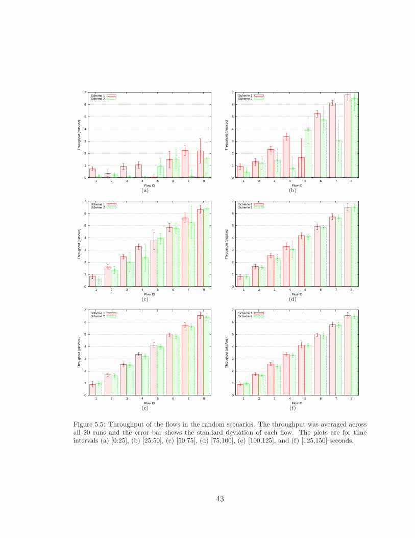
simulation. . . . . . . . . . . . . . . . . . . . . . . . . . . . . . . . . . 385.5 Throughput of the flows in the random scenarios. . . . . . . . . . . . 43

vii

CHAPTER 1

INTRODUCTION

1.1 Ad Hoc Networking and Cross-Layer Algorithms

It is difficult to walk down the street in the developed world and not spot some

sort of wireless communication device in action. It could be any number of things:

cell-phone, wireless-enabled laptop, Bluetooth headset, in-car GPS device, portable

video game system, etc. Wireless connectivity has been changing from a consumer

convenience to a consumer necessity. This trend is also apparent in other sectors

such as military, corporate, medical, manufacturing, etc. With so many devices

already out there and many more to come, it is desirable that these devices be able

to communicate with one another, thus creating an ad hoc network. These devices

will want to communicate with minimal delay and maximum throughput. It is the

job of most ad hoc networking protocols to provide such a solution, and it is the goal

of this thesis.

When searching for a solution for a good networking algorithm which has the

aforementioned properties, it does not take long to discover the complexity involved.

The classical approach is to break down the networking problem into smaller parts,

called layers, and then optimize them individually. This modularization process serves

its purpose well—to break down the problem into smaller, more-manageable pieces—

however, all of this comes at the cost of overall optimization. By designing the layers

exclusive of one another, the chances of the whole system being optimal are slim. Due

to this sub optimality of the layered approach, we will focus on cross-layer networking

solutions.

1

1.2 From Theory to Simulation

Many, if not all, electronic devices available on the market today are the indirect

result of abstract theoretical works. The theories of which these products are the

result are often based upon oversimplified models of the actual problem. However,

that does not discredit the theory, but only makes the jump from theory to imple-

mentation tougher because the designer has to be able to (i) discover the stated and

unstated simplifications and (ii) find ways to overcome them. In overcoming these

simplifications, the designer has to make compromises that may hurt the theoretical

performance while making the system more practical. In this thesis, we serve as the

designers and try to find the delicate balance between practicality and performance.

The theoretical work, which we will discuss in more detail in Chapter 2, has proven

that there exists a centralized scheduler which will provide maximal throughput. The

scheduler uses the queue-length information of all nodes to schedule transmissions

and transmission rates. In addition to providing maximal throughput, the scheduler

guarantees the stability of the queues.

The congestion controller in [1], upon which our work is based, works to provide

fairness for all flows by using the queue lengths to determine the flow rate at the

application layer. The “cross-layer” term is due to the fact that the congestion con-

troller is usually implemented at the transport layer and the queue length is found at

the medium access (MAC) layer.

In this thesis, we take the scheduler and congestion controller and apply the the-

ory to a decentralized protocol and simulate the protocol in the Network Simulator

(NS2) [2].

1.3 Outline of Thesis

In Chapter 2, we provide the reader with some background materials, such as the

802.11 Distributed Coordination Function, and some related works in the areas of

2

priority scheduling and backpressure-based scheduling. In Chapter 3, we summarize

the system notation and the theoretical findings upon which this thesis is based. Then,

in Chapter 4, we describe the design of a distributed backpressure-based scheduler and

congestion controller. In Chapters 5 and 6 we discuss and analyze the performance of

the distributed system, then summarize this thesis and suggest areas for future work.

3

CHAPTER 2

BACKGROUND AND RELATED WORK

2.1 802.11 Distributed Coordination Function (DCF)Medium Access Method

This work involves an adaptation of the 802.11 Distributed Coordination Function

(DCF) medium access control (MAC) mode. The 802.11 standard describes two MAC

modes: the DCF and Point Coordination Function (PCF) modes. The coordination

functions control access to the wireless medium. The PCF mode is for infrastructure-

based networks and is not discussed in this thesis (for further information on the

PCF mode, refer to [3] or [4]). The DCF, on the other hand, is designed mainly for

infrastructure-less networks and is what this thesis involves. The DCF mode allows

many independent nodes to access the same wireless medium without the aid of a

central entity. The mode uses a carrier sense multiple access (CSMA) scheme and

collision avoidance (CA) to help access the medium while avoiding collisions. This

type of system is referred to as CSMA/CA.

When trying to access the medium using the DCF mode, the node will always be

performing carrier sensing. Carrier sensing is simply the act of sensing the channel

to see if there is a transmission currently taking place or not. The carrier sensing

will decide whether the channel is idle or busy. If carrier sensing finds the channel

idle, then the node can contend for access to the channel. However, in DCF mode, a

node cannot simply transmit whenever the channel is deemed idle; it must wait for a

period of time referred to as the backoff window, or contention window.

Once a node gets a packet to send and wants to access the medium, it will first

4

choose a value for its backoff interval, which we will refer to as b. This value is chosen

randomly on the interval [0, CWmin], where CWmin is a constant. We will refer to

this interval as the contention window interval (CWI) and we will use the symbols

CWlb and CWub for the lower and upper bounds. The window corresponds to slots

and a slot corresponds to a real time, which we will refer to as slot time. So, once

the node carrier senses the channel as idle, it will then start decrementing b every

slot time seconds. As long as the channel stays idle, the node will keep decrementing

b until it gets to 0, and it will then send out its frame.1 If there is no collision, then

the receiving node will reply with an acknowledgment. Otherwise, the transmitting

node will deem that a collision has taken place and exponentially increase its CWI

upper bound, CWub, by multiplying it by two. The CWI upper bound is calculated

according to

CWub = 2log2(CWmin+1)+i − 1, i ≤ log2(CWmax + 1)− log2(CWmin + 1), (2.1)

where i is the number of consecutive collisions, CWmin = min(CWub) and CWmax =

max(CWub). For example, if CWmin = 31 and CWmax = 1023, then i ≤ 5 and as

long as collisions happen, CWub will evolve as follows: 31, 63, 127, 255, 511, 1023.

Also, we should mention the interframe spacing (IFS). The two interframe spacings

of interest are the DCF interframe space (DIFS) and the short interframe space

(SIFS). The DIFS is the minimum idle time required before nodes can have immediate

access to the medium. The SIFS is shorter than DIFS and is intended for use by high

priority packets, such as positive acknowledgements.

We will wrap up our overview of the 802.11 DCF with a short example, shown in

Figure 2.1. In this example, we have three nodes A, B, and C and let CWmin = 7.

At t0, both A and C get a packet from their upper layers to send to B. Nodes A and

C then calculate backoff b over the interval [0, 7], and they both happen to choose 4

1We assume that the RTS/CTS virtual carrier sensing method is not used here.

5

in this case. At t1, all nodes sense the channel is idle. After waiting for the DIFS

period, both A and C start counting down. At t2, both A and C have counted down

to 0, and they both transmit their data frames, which causes a collision. Since B

could not receive either data frame due to the collision, no acknowledgement is sent.

At t3, both A and C have not received an acknowledgement and assume a collision

has occurred. Using the new upper bound in (2.1), they recalculate their backoff b in

the interval [0, 15]. We will assume A chooses 3 and C chooses 5. Once again, both A

and C start to countdown. At t4, A reaches 0 and retransmits its data frame. Node

B then receives the data frame from A, waits for an SIFS period, and at t5, sends an

acknowledgement. After waiting for a DIFS period, node C restarts its countdown

at t6, and then after counting down to 0, sends its data frame to B, which is then

acknowledged.

Figure 2.1: A simple example showing some properties of the 802.11 DCF MAC access mode. Thesmall rectangles with the numbers above them represent backoff slots and are of duration slot time.

2.2 802.11 Priority Schemes

In [5], the authors propose a priority scheme for the DCF access method of 802.11.

They provide four priority levels. Two levels are created by changing the interframe

spacing (IFS). In 802.11 DCF, once the channel has been declared idle by the carrier

sensing mechanism, the node will wait for a DIFS period before starting to decrement

6

its backoff counter. Deng and Chang [5] decided to create two DIFS period values,

one for priority traffic, PIFS, and one for regular traffic, DIFS, where a PIFS period

was shorter than a DIFS period. Thus, if two nodes had the same backoff value and

sensed the channel as being idle at the same time, but one had a priority packet

and the other did not, then the node with the priority packet would start counting

down first and thus have a better chance of sending its priority packet before the

regular packet. The second method of providing priority was via the backoff counter.

In the regular 802.11 DCF, a packet would choose a random backoff value from the

CWI (0, CWub), where CWub is calculated according to (2.1). To create prioritization,

Deng et. al change the CWI to (0, CWub

2) for high priority packets and (CWub

2, CWub)

for low priority packets. Thus, assuming no collisions, the high priority packets are

guaranteed a lower backoff value b.

In [6], Xiao creates another priority scheme based upon the backoff mechanism.

The author uses the following three metrics to differentiate the priority ith class: the

initial window size Wi,0, the window-increasing factor σi, and the maximum back-

off stage mi, where σi is the factor by which the current window size is increased

when a transmitted packet frame collides. In the 802.11 standard, the initial window

size (Wi,0) is equal to 31, the window increasing factor (σi) is 2, and the maximum

backoff stage (mi) is 6. In this scheme, class i’s backoff window is calculated by

bx · d(σi)jWi,0ec, where x is a uniform random variable in (0, 1), j is the number of

consecutive times a station tries to send a frame, byc represents the largest integer

less than or equal to y, and dye represents the smallest integer greater than or equal

to y. If priority class i has a higher priority than class j, then the authors declare

Wi,0 ≤ Wj,0, 1 < σi ≤ σj, and mi ≤ mj.

In [7], Vaidya et al. construct an algorithm to emulate Self-Clocked Fair Queuing

(SCFQ) in a distributed manner. Given weights for each traffic flow, the goal is to

have the throughput proportional to that weight. For example, if φi is the weight for

7

flow i and Ti is the throughput for flow i, then the equality

Ti

Tj

=φi

φj

, ∀i, j (2.2)

should be maintained, assuming that both flows i and j are backlogged. As in the

previous schemes, this also prioritizes traffic via an intelligent choice of the initial

backoff interval, which reflects the weighting of the flow. However, this scheme,

unlike [5] and [6] which simply prioritize traffic, attempts to achieve an actual ratio

reflecting the weights of the flows, as seen in (2.2).

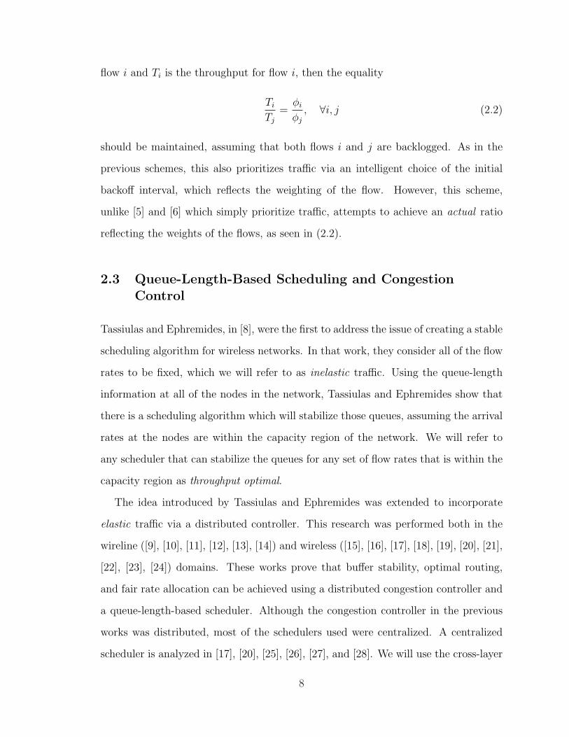
2.3 Queue-Length-Based Scheduling and CongestionControl

Tassiulas and Ephremides, in [8], were the first to address the issue of creating a stable

scheduling algorithm for wireless networks. In that work, they consider all of the flow

rates to be fixed, which we will refer to as inelastic traffic. Using the queue-length

information at all of the nodes in the network, Tassiulas and Ephremides show that

there is a scheduling algorithm which will stabilize those queues, assuming the arrival

rates at the nodes are within the capacity region of the network. We will refer to

any scheduler that can stabilize the queues for any set of flow rates that is within the

capacity region as throughput optimal.

The idea introduced by Tassiulas and Ephremides was extended to incorporate

elastic traffic via a distributed controller. This research was performed both in the

wireline ([9], [10], [11], [12], [13], [14]) and wireless ([15], [16], [17], [18], [19], [20], [21],

[22], [23], [24]) domains. These works prove that buffer stability, optimal routing,

and fair rate allocation can be achieved using a distributed congestion controller and

a queue-length-based scheduler. Although the congestion controller in the previous

works was distributed, most of the schedulers used were centralized. A centralized

scheduler is analyzed in [17], [20], [25], [26], [27], and [28]. We will use the cross-layer

8

congestion control and scheduling framework developed in the works mentioned as a

foundation for this thesis.

9

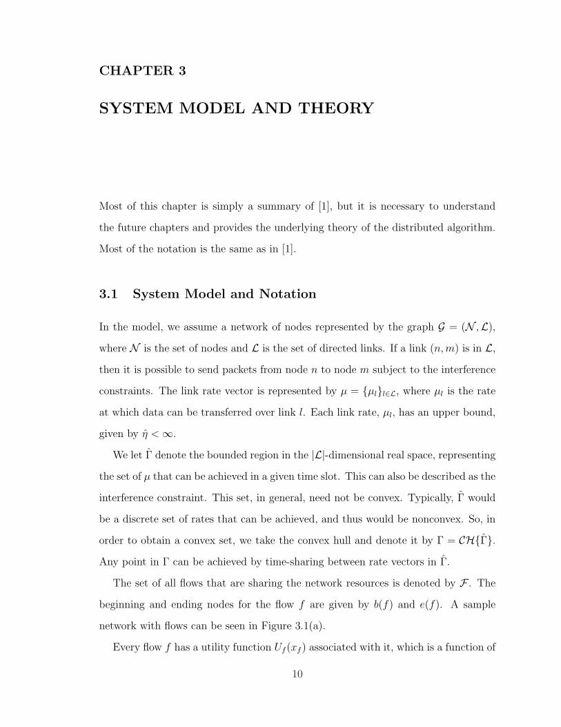
CHAPTER 3

SYSTEM MODEL AND THEORY

Most of this chapter is simply a summary of [1], but it is necessary to understand

the future chapters and provides the underlying theory of the distributed algorithm.

Most of the notation is the same as in [1].

3.1 System Model and Notation

In the model, we assume a network of nodes represented by the graph G = (N ,L),

where N is the set of nodes and L is the set of directed links. If a link (n,m) is in L,

then it is possible to send packets from node n to node m subject to the interference

constraints. The link rate vector is represented by µ = {µl}l∈L, where µl is the rate

at which data can be transferred over link l. Each link rate, µl, has an upper bound,

given by η < ∞.

We let Γ denote the bounded region in the |L|-dimensional real space, representing

the set of µ that can be achieved in a given time slot. This can also be described as the

interference constraint. This set, in general, need not be convex. Typically, Γ would

be a discrete set of rates that can be achieved, and thus would be nonconvex. So, in

order to obtain a convex set, we take the convex hull and denote it by Γ = CH{Γ}.Any point in Γ can be achieved by time-sharing between rate vectors in Γ.

The set of all flows that are sharing the network resources is denoted by F . The

beginning and ending nodes for the flow f are given by b(f) and e(f). A sample

network with flows can be seen in Figure 3.1(a).

Every flow f has a utility function Uf (xf ) associated with it, which is a function of

10

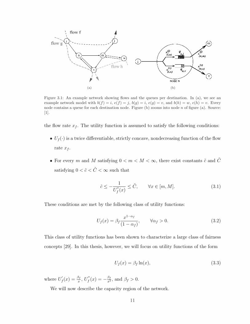
(a) (b)

Figure 3.1: An example network showing flows and the queues per destination. In (a), we see anexample network model with b(f) = i, e(f) = j, b(g) = i, e(g) = v, and b(h) = w, e(h) = v. Everynode contains a queue for each destination node. Figure (b) zooms into node n of figure (a). Source:[1].

the flow rate xf . The utility function is assumed to satisfy the following conditions:

• Uf (·) is a twice differentiable, strictly concave, nondecreasing function of the flow

rate xf .

• For every m and M satisfying 0 < m < M < ∞, there exist constants c and C

satisfying 0 < c < C < ∞ such that

c ≤ − 1

U′′f (x)

≤ C, ∀x ∈ [m,M ]. (3.1)

These conditions are met by the following class of utility functions:

Uf (x) = βfx1−αf

(1− αf ), ∀αf > 0. (3.2)

This class of utility functions has been shown to characterize a large class of fairness

concepts [29]. In this thesis, however, we will focus on utility functions of the form

Uf (x) = βf ln(x), (3.3)

where U′f (x) =

βf

x, U

′′f (x) = −βf

x2 , and βf > 0.

We will now describe the capacity region of the network.

11

Definition 1 (Capacity Region). The capacity region Λ of the network contains the

set of flow rates {xf}f∈F ≥ 0 for which there exists a set{

µ(d)l

}d∈N

l∈Lthat satisfies

•[∑

d

µ(d)l

]∈ Γ, where µ

(d)l ≥ 0 for all l ∈ L, d ∈ N .

• µ(d)into(n) +

∑

f

xfI{b(f)=n,e(f)=d} ≤ µ(d)out(n) for each n ∈ N , and d 6= n, where

µ(d)into(n) :=

∑

(k,n)∈Lµ

(d)(k,n) and µ

(d)out(n) :=

∑

(n,m)∈Lµ

(d)(n,m). Notice that µ

(d)into(n) (or

µ(d)out(n)) denotes the potential number of packets that are destined for node d,

incoming to (or outgoing from) node n. Here, Ia=b is the identity function,

where Ia=b = 1 if a = b and Ia=b = 0 if a 6= b.

At every node, there is a queue for each flow having the same destination. We

will use qn,d[t] to denote the number of packets that are destined for node d, waiting

for service at node n at time t. Figure 3.1(b) shows an example of such queues. The

evolution of the queues is then given by

qn,d[t+1] = qn,d+∑

f

xf [t]I{b(f)=n,e(f)=d}+s(d)into(n)−s

(d)out(n)[t], ∀n ∈ N , d ∈ N \{n},

(3.4)

where s(d)into(n) :=

∑

(k,n)∈Ls(d)(k,n) and s

(d)out(n)[t] :=

∑

(n,m)∈Ls(d)(n,m), and s

(d)(n,m) denotes the

rate provided to d-destined packets over link (n,m) at slot t (a slot is 1 unit time).

It is important to note the distinction between s and µ: s(d)(n,m)[t] denotes the actual

amount of packets served over the link, whereas µ(d)(n,m)[t] denotes the potential amount

served. Thus, s(d)(n,m)[t] = min(µ

(d)(n,m)[t], qn,d[t]) for all (n,m) ∈ L, d 6= n. We also let

s(n,m)[t] =∑

d sd(n,m[t], which is the total amount of traffic served over link (n, m). We

will refer to the queues with destinations, qn,d, as queue’s-per-destination, or QPDs.

Also, the sum of all QPDs at a given node will be called the overall queue, or OQ.

12

3.2 Problem Statement and Optimal Point

The goal of Eryilmaz et al. in [1] was to design a congestion control, scheduling

mechanism such that the flow rate vector x solves the following optimization problem:

maxx∈Λ

∑

f∈FUf (xf ). (3.5)

Due to the strict concavity assumption of Uf (·) and the convexity of the capacity

region Λ, there does exist a unique optimizer to (3.5), which we will further refer to

as x?, or the fair rate allocation point. We will also refer to an element out of x? as

x?f .

3.3 Backpressure-Based Centralized Scheduling Algorithm

Introduced by Tassiulas and Ephremides [8], the centralized scheduling algorithm

upon which our work is based is known as the back-pressure scheduler. This scheduler

uses the differential backlog at the two end-nodes of a link to determine the rate of

that link. The idea behind the scheduler can be explained simply. Assume we have

a flow f which must take a route consisting of three nodes: (na → nb → nc). The

idea behind the backpressure based scheduler is to schedule traffic such that, in this

case, the middle node nb does not get overloaded with packets from na, but will have

a similar link rate from nb → nc as the link na → nb. By doing so, the queues at na

and nb will be stable and the traffic over the links will also be stable.

Definition 2 (Back-pressure Scheduler). At slot t, for each (n,m) ∈ L, we define the

differential backlog for destination node d as W(n,m),d[t] := (qn,d[t]− qm,d[t]). Also, we

let W(n,m)[t] = maxd

{W(n,m),d[t]

}and d(n,m)[t] = arg max

d

{W(n,m),d

}. Then, choose

13

the rate vector µ[t] ∈ L that satisfies

µ[t] ∈ arg max{η∈Γ}

∑

{(n,m)∈L}η(n,m)W(n,m)[t], (3.6)

then serve the queue holding packets destined for node d(n,m)[t] over link (n,m) at

rate µ(n,m)[t]. Effectively, this is setting µ(d(n,m)[t])

(n,m) [t] = µ(n,m)[t]. The rest of the queues

at node n are not served at slot t.

3.4 Congestion Controller

Definition 3 (Congestion Controller). At the beginning of time slot t, each flow, say

f , has access to the queue length of its first node, qb(f),e(f)[t]. The data rate xf [t] of

flow satisfies

xf [t + 1] ={xf [t] + α(KU ′(xf [t])− qb(f),e(f)[t])

}M

m, (3.7)

where the notation yba projects the value of y to the closest point in the interval [a, b].

We assume that m is a fixed positive valued quantity that can be arbitrarily small,

M > 2η, and K > 0.

In [1], the authors prove the following theorem, which shows that the average rate

obtained for each flow can be made arbitrarily close to its fair share, according to

(3.5), by choosing a sufficiently large K.

Theorem 1. For α = (1/K)2, and for some finite B > 0, we have: for all f ∈ F

x?f −

B√K≤ lim inf

T→inf

1

T

T−1∑t=0

xf [t] ≤ lim supT→inf

1

T

T−1∑t=0

xf [t] ≤ x?f +

B√K

. (3.8)

14

CHAPTER 4

DESIGN OF DISTRIBUTED CONTROLLER

AND SCHEDULER

In this chapter, we will first discuss our simulation tool and then discuss the design

and implementation of the scheduler and congestion controller.

4.1 NS2 and MIRACLE

The Network Simulator [2], which we will further refer to as NS2, is an open source

discrete event simulator aimed at networking research. NS2 is comprised of two parts:

an object oriented simulator, written in C++, and an interpreter, written in object

oriented Tool Command Language (OTcl). The simulator portion is built for speed

and allows simulations with tens to hundreds of nodes with hundreds of flows to take

less than real time. The interpreter, on the other hand, is meant for the user to be

able to have access to all aspects of the scenario (network topology, traffic generation,

protocol parameters) without having to change and recompile the C++ code.

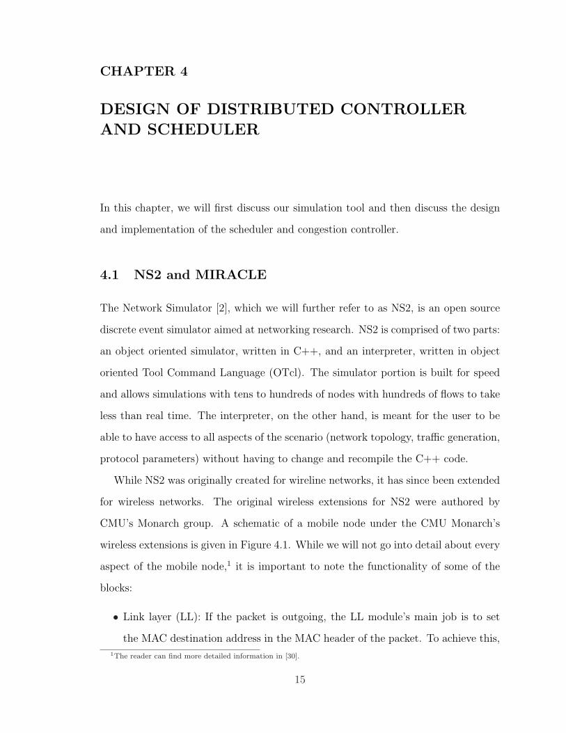
While NS2 was originally created for wireline networks, it has since been extended

for wireless networks. The original wireless extensions for NS2 were authored by

CMU’s Monarch group. A schematic of a mobile node under the CMU Monarch’s

wireless extensions is given in Figure 4.1. While we will not go into detail about every

aspect of the mobile node,1 it is important to note the functionality of some of the

blocks:

• Link layer (LL): If the packet is outgoing, the LL module’s main job is to set

the MAC destination address in the MAC header of the packet. To achieve this,

1The reader can find more detailed information in [30].

15

LL

IFq

MAC

NetIF

RadioPropagationModel

Channel

Src/Sink

ARP

arptable_

uptarget_

uptarget_channel_

propagation_

uptarget_downtarget_

downtarget_

downtarget_

uptarget_

demuxport

entry_

demuxaddr

defaulttarget_RTagent

(DSDV)

255IP address

mac_

target_

Figure 4.1: Schematic of a mobile node under the CMU Monarch’s wireless extensions. Source: [2].

there is an ARP module connected to it which will perform the Internet protocol

(IP) destination address to MAC hardware address conversion. Once the MAC

address has been placed in the header, the packet is passed down to the IFq.

• Address resolution protocol (ARP): The ARP module receives requests from

the LL wanting MAC addresses resolved from IP addresses. If the ARP module

already has a MAC address for the corresponding IP address, then it immediately

responds with that MAC address. If not, it immediately broadcasts an ARP

query and caches the packet temporarily.

• Interface queue (IFq): The IFq is a simple queue module with priority for control

packets. If the IFq receives a control packet such as a routing protocol packet,

it will immediately put it at the head of the queue. Some aspects of this module

will later be modified to implement the scheduler.

• Medium access control (MAC): The 802.11 DCF MAC has been implemented

in this module by the CMU Monarch team. It implements both virtual and

physical carrier sensing and uses the RTS/CTS/DATA/ACK pattern for unicast

16

packets and just DATA for broadcast packets. Some aspects of this module will

later be modified to implement the scheduler.

In order to keep a strict modularized network stack, most layers in NS2 are only

designed to send packets up or down with no other communication between layers

taking place. In the system in this work, cross-layer communication is important and

necessary for easy implementation. Thus, the Multi-Interface Cross-Layer Extension

library for the Network Simulator (NS-MIRACLE) [31] was used.

NS-MIRACLE is a set of libraries which extend NS2 and allow for easy exchange of

messages from one layer to another (cross-layer messages). NS-MIRACLE also allows

for placing multiple modules at each layer (e.g., multiple physical layer modules to

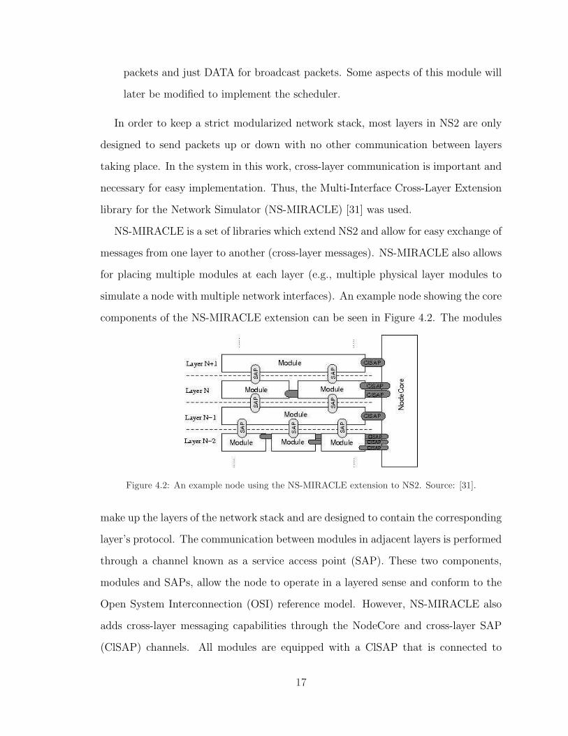
simulate a node with multiple network interfaces). An example node showing the core

components of the NS-MIRACLE extension can be seen in Figure 4.2. The modules

Figure 4.2: An example node using the NS-MIRACLE extension to NS2. Source: [31].

make up the layers of the network stack and are designed to contain the corresponding

layer’s protocol. The communication between modules in adjacent layers is performed

through a channel known as a service access point (SAP). These two components,

modules and SAPs, allow the node to operate in a layered sense and conform to the

Open System Interconnection (OSI) reference model. However, NS-MIRACLE also

adds cross-layer messaging capabilities through the NodeCore and cross-layer SAP

(ClSAP) channels. All modules are equipped with a ClSAP that is connected to

17

the NodeCore. The NodeCore serves as a cross-layer bus that will carry cross-layer

messages from any module to any other module. The cross-layer messages are also

fully customizable to allow the designer maximum flexibility.

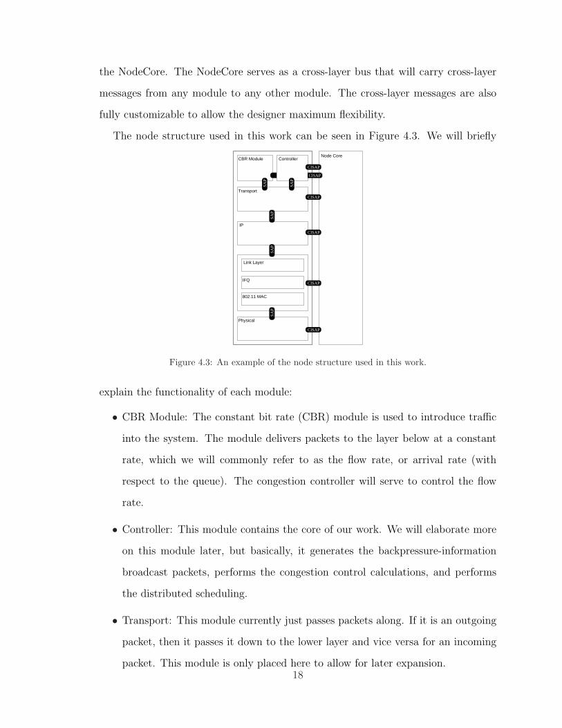
The node structure used in this work can be seen in Figure 4.3. We will briefly

CBR Module ControllerNode Core

Transport

IP

Link Layer

IFQ

Physical

802.11 MAC

SAP

SAP

SAP

ClSAP

ClSAP

ClSAP

ClSAP

ClSAP

SAP

SAP

ClSAP

Figure 4.3: An example of the node structure used in this work.

explain the functionality of each module:

• CBR Module: The constant bit rate (CBR) module is used to introduce traffic

into the system. The module delivers packets to the layer below at a constant

rate, which we will commonly refer to as the flow rate, or arrival rate (with

respect to the queue). The congestion controller will serve to control the flow

rate.

• Controller: This module contains the core of our work. We will elaborate more

on this module later, but basically, it generates the backpressure-information

broadcast packets, performs the congestion control calculations, and performs

the distributed scheduling.

• Transport: This module currently just passes packets along. If it is an outgoing

packet, then it passes it down to the lower layer and vice versa for an incoming

packet. This module is only placed here to allow for later expansion.18

• IP: The IP module performs the routing. The packets generated from the CBR

module have a destination address and the IP module converts that address to

a next-hop address. Once the next-hop address has been placed in the packet

header, the packet is sent on to the lower layer. If the packet is an incoming

packet, the IP layer first figures out if this node is the final destination or not. If

so, the packet is passed on to the upper layer. If not, the node needs to forward

this packet on, so the next-hop address is placed into the header and the packet

is then sent on to the lower layer.

• MAC: This module contains three NS2 components, the Link Layer (LL), the

interface queue (IFQ), and the 802.11 MAC. These are the same components

shown in Figure 4.1 and explained above.

• Physical (PHY): The Physical (PHY) module performs some simple signal to

interference plus noise (SINR) threshold testing to decide whether or not packets

have been correctly received.

4.2 Distributed Congestion Controller

The congestion controller is discussed in Section 3.4 and updates the flow rate itera-

tively based upon the current queue length at the source node and the derivative of

the utility of the flow. In order to avoid large oscillations of the flow rate, we will use

a modified version of (3.7), given by

xf [t + ∆cc] ={xf [t] + α(KU ′(xf [t])− qb(f),e(f)[t])

}M ′

m′ , (4.1)

where m′ = max{m,xf [t]

2}, M ′ = min{M, 2xf [t]}, m and M are constant scalars, and

∆cc is the time between rate updates. In most of our simulations, m = 1 pkts/sec

and M = 200 pkts/sec. The m′ and M ′ serve to put hard limits on the rate of change

and their need will be shown in the next section. Similar ideas are implemented in

19

versions of the transport control protocol (TCP).

In our NS2 model, we place the congestion controller in the Controller module, as

shown in Figure 4.3. Every ∆cc seconds, the Controller sends a cross-layer message

(ClMessage) to the MAC module, requesting the current queue length. When the

MAC module receives that query, it immediately responds with another ClMessage

which contains the current queue length for the flow, or flows, being generated by

this node. Once the Controller receives the ClMessage containing the queue length, it

updates the rate according to (4.1) and then sends a ClMessage to the CBR module

which contains the updated rate. On receipt of the rate update ClMessage, the CBR

module will then update its timer to accurately reflect the new flow rate.

The CBR module generates packets every ∆CBR s, where ∆CBR = packetSizexf

. The

module uses a timer to schedule packet generation. When the timer expires, a packet

is sent to the layer below. When a rate update cross-layer message is received from

the Controller, the CBR timer is updated according to

Tnp = max (∆new − (tc − tlp), 0) , (4.2)

where Tnp is the time until the next packet generation, ∆new is the new packet interval,

tc is the current time, and tlp is the time the last packet was generated. So, after this

update, the next packet will be scheduled to be generated in Tnp s, or at simulation

time tc + Tnp.

4.2.1 Optimal flow rate

Later in our simulations, it will be valuable to know what the optimal fair rate allo-

cation is for certain scenarios. Let us start with a simple scenario with four flows and

calculate the optimal flow rates using Lagrange multipliers. Let f(x1, x2, x3, x4) be

the function which we are trying to optimize and let g(x1, x2, x3, x4) be the constraint.

Recall that our optimization problem is maxx

∑f U(xf ), where xf is the flow rate of

20

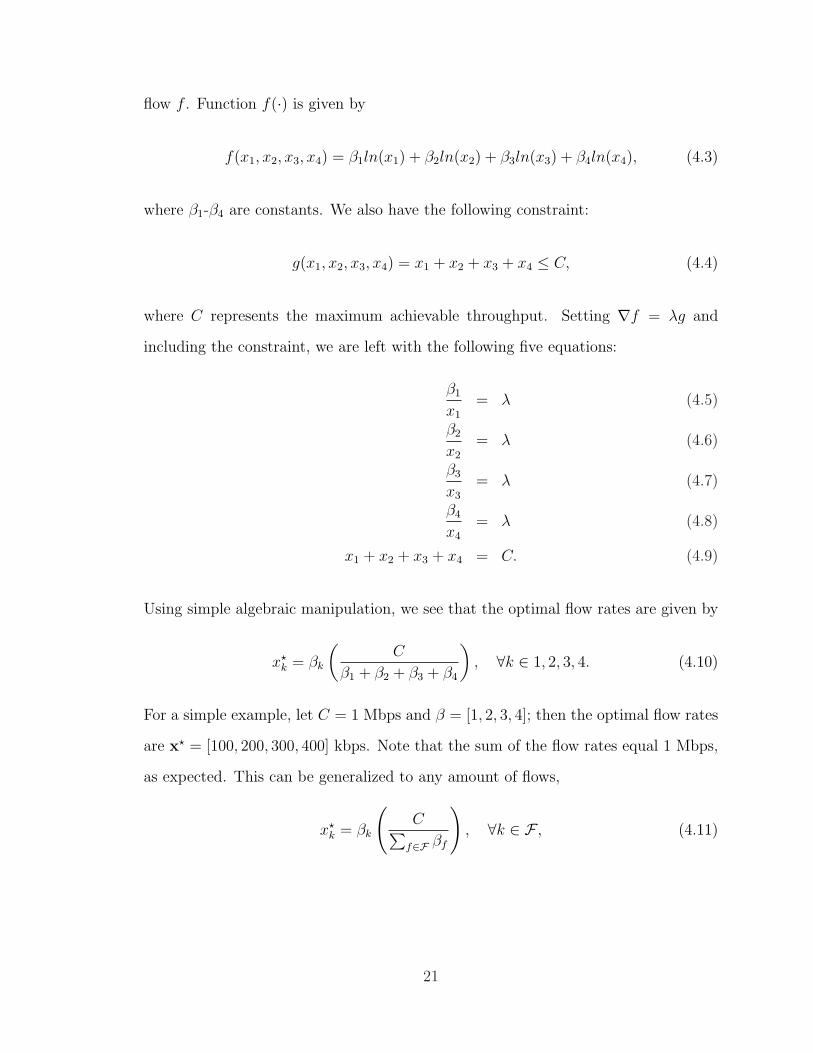
flow f . Function f(·) is given by

f(x1, x2, x3, x4) = β1ln(x1) + β2ln(x2) + β3ln(x3) + β4ln(x4), (4.3)

where β1-β4 are constants. We also have the following constraint:

g(x1, x2, x3, x4) = x1 + x2 + x3 + x4 ≤ C, (4.4)

where C represents the maximum achievable throughput. Setting ∇f = λg and

including the constraint, we are left with the following five equations:

β1

x1

= λ (4.5)

β2

x2

= λ (4.6)

β3

x3

= λ (4.7)

β4

x4

= λ (4.8)

x1 + x2 + x3 + x4 = C. (4.9)

Using simple algebraic manipulation, we see that the optimal flow rates are given by

x?k = βk

(C

β1 + β2 + β3 + β4

), ∀k ∈ 1, 2, 3, 4. (4.10)

For a simple example, let C = 1 Mbps and β = [1, 2, 3, 4]; then the optimal flow rates

are x? = [100, 200, 300, 400] kbps. Note that the sum of the flow rates equal 1 Mbps,

as expected. This can be generalized to any amount of flows,

x?k = βk

(C∑

f∈F βf

), ∀k ∈ F , (4.11)

21

and the optimal value of the summation can be given by

∑

f

U(x?f ) =

∑

k∈Fβk ln

(βk

(C∑

f∈F βf

)). (4.12)

4.3 Distributed Backpressure-Based Scheduler

The goal of the backpressure scheduler is to normalize the queues in the network. The

centralized scheduler in Section 3.3 uses the differential backlog at the end nodes of a

link, i.e., the backpressure, to determine the rate of that link. Effectively, it provides

a high rate to those nodes with the highest backpressure in the network. By assigning

a higher rate to those nodes with a high backpressure, the scheduler is attempting to

decrease the backpressure at those nodes and, in turn, normalize the queues of the

network.

The centralized scheduler is proven to work, but we are interested in a scheduler

that is distributed and does not need information about every node in the network.

In order to do so, the following two main questions must be answered:

• How is the backpressure information going to be obtained?

• Once the backpressure has been obtained, how is the node going to use that

information?

For the first item, each node will periodically send out a broadcast packet contain-

ing its own queue information, as well as its backpressure information. The recipient

of this broadcast packet can then (i) calculate its own backpressure using the queue

length of the sending node, and (ii) compare backpressure values with the neighboring

node. The format of an example broadcast packet can be seen in Table 4.1. Accord-

ing to the example packet, at node n, qn,m1 = 5, qn,m2 = 40, qn,m3 = 10, Wn,m1 = 2,

Wn,m2 = 25, and Wn,m3 = 0, where Wn,d = (qn,d − qx,d) with x representing the next

hop for packets destined for d.

22

Table 4.1: Sample broadcast packet from node n which has packets destined for m1, m2, and m3.

Destination Queue Length Backpressure(2 bytes) (2 bytes) (2 bytes)

m1 5 2m2 40 25m3 10 0

Upon arrival of that broadcast packet from n, the receiving node, say r, does two

things. First, r checks to see if n is the next hop for any of the destinations for which

it has queues. If so, r then calculates the backlog. So, continuing with the example, if

there is a flow with route r-n-(· · · )-m2, then when r receives the broadcast packet, it

will update its backpressure to W(r,n),m2 = qr,m2 − qn,m2 = qr,m2 − 40. Secondly, r will

take the maximum backpressure from the packet, maxd Wn,d, and update its neighbor

backpressure table (NBT). The NBT is simply a table containing the neighbor’s ID

and its maximum backpressure. A neighbor is added any time a broadcast is received

from that node. A sample for r can be seen in Table 4.2.

Table 4.2: A sample neighbor backpressure table (NBT) for node r.

Neighbor (N) Backpressure (W )n 22N2 32N3 13N4 0

Assuming that r has the backpressure values for all of r’s neighbors, r now has

to decide how to use those backpressure values. This brings us to the second item,

that is, how to use the local backpressure values. In the centralized scheme, link rates

are chosen according to (3.6), a maximization of a weighted sum. This maximization

would most likely result in the links with high backpressure getting high link rates

alloted to them and vice versa with links with low backpressure.

Using this basic concept, we developed a distributed scheduler on top of the 802.11

MAC. As explained in Section 2.1, the 802.11 DCF chooses a random backoff value

when it has a packet to transmit. This backoff value was created to deal with con-

23

tention in the network. Depending on the level of contention in the network, the

backoff value may be either large (high contention) or small (low contention). In

addition, a node with a small backoff value will have faster access to the channel than

a node with a large backoff value. It is simple to see that this value can be used as a

priority mechanism for channel access. For example, if a node has high (low) priority

traffic then it can set its backoff value low (high). By doing so, it is more likely that

the high priority traffic will obtain a higher throughput. Some prior 802.11 priority

schemes are mentioned in Section 2.2.

The goal of our scheduler is to allow nodes with high backpressure to transmit

more often than nodes with low backpressure. To do so, we will take advantage of

802.11 DCF backoff value and treat the backpressure as a priority value, where a high

backpressure represents high priority traffic.

As explained in Section 2.1, the backoff value (b) is chosen uniformly on the interval

[CWlb, CWub], where CWlb = 0 in the 802.11 standard, and CWub evolves according

to (2.1). With the goal of prioritizing based on backpressure, we have created the

following two schemes for our scheduler:

1. This scheme simply changes CWmin based upon the backpressure values of the

node in question, n, and its neighbors, nbr(n). The node first calculates the

minimum and maximum backpressure values among itself and its neighbors:

Wmax = max(k,m)

k∈{nbr(n),n}

{W(k,m)}

Wmin = min(k,m)

k∈{nbr(n),n}

{W(k,m)}.

Then, it sets its contention window minimum value according to

CWmin = (CWumax − CWumin)

(1− W −Wmin

Wmax −Wmin

)+ CWumin, (4.13)

where CWumin and CWumax are user-supplied values that set the minimum and

24

maximum CWub, CWumax ≥ CWumin, and W = maxm W(n,m). Basically, this is

a simple linear mapping function that maps high backpressure to low contention

window values. For example, if W = Wmax, then CWmin = CWumin and the

node will pick a b along the interval [0, CWumin]. Likewise, if W = Wmin, then

the node will pick a b along the interval [0, CWumax]. In this scheme, CWlb = 0

always and CWub evolves according to (2.1), but with CWmin changing.

2. This scheme is loosely based on [5] and changes both CWub and CWlb. In scheme

1, there is a nonzero probability that a node with CWmin = 255, for example,

could gain access to the channel before a node with CWmin = 31 because b is

chosen over the interval [0, CWub]. We will use a similar mapping as the other

schemes, but use the value calculated as a mean value. That is,

CWavg = (CWumax − CWumin)

(1− W −Wmin

Wmax −Wmin

)+ CWumin (4.14)

and

CWlb = max {CWavg − σ, 0} (4.15)

CWub = CWavg + σ. (4.16)

As an example case, let us assume that Wmax = 200, Wmin = 50, and W = 75.

Also, let CWumax = 511 and CWumin = 31. This would result in CWavg = 431.

Further, letting σ = 10, we have CWlb = 421 and CWub = 441. So, in this

scheme, b would be chosen randomly from the interval [421,441], whereas in

scheme 1 it would be chosen from [0,431].

25

CHAPTER 5

SIMULATIONS AND ANALYSIS OF

DISTRIBUTED ALGORITHM

5.1 Scenarios

Before we go through the simulations we have performed, we will first clearly explain

the general scenario layouts for our simulations. When these scenarios are referred

to later, assume that everything is exactly the same as explained here, unless it is

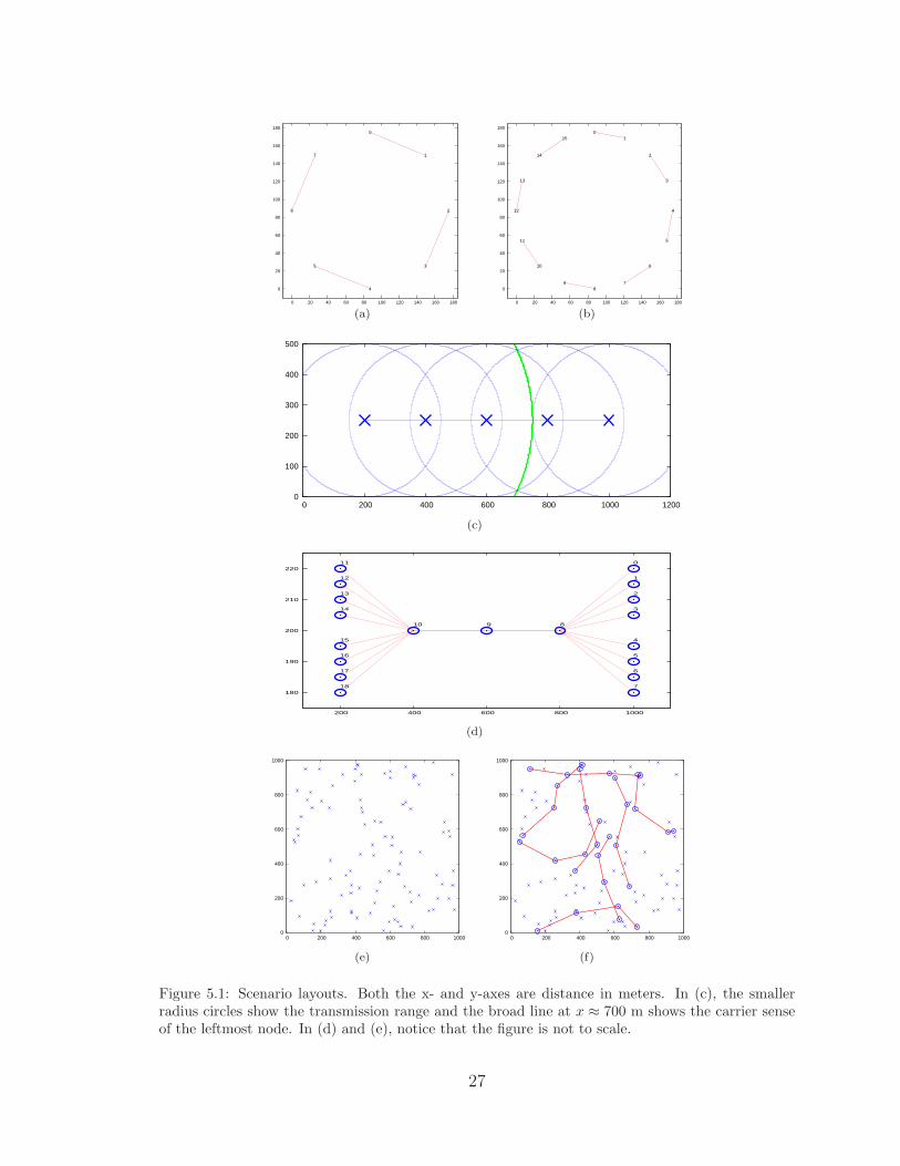
specifically stated otherwise. All the scenarios can be seen in Figure 5.1.

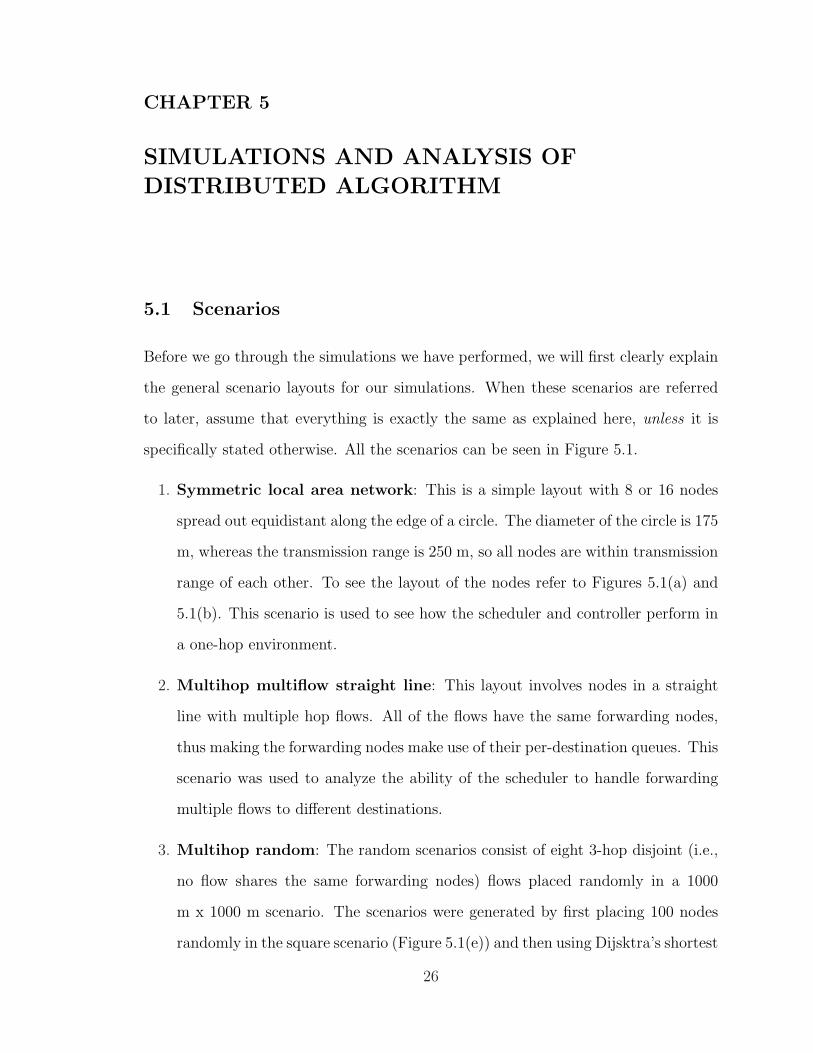
1. Symmetric local area network: This is a simple layout with 8 or 16 nodes

spread out equidistant along the edge of a circle. The diameter of the circle is 175

m, whereas the transmission range is 250 m, so all nodes are within transmission

range of each other. To see the layout of the nodes refer to Figures 5.1(a) and

5.1(b). This scenario is used to see how the scheduler and controller perform in

a one-hop environment.

2. Multihop multiflow straight line: This layout involves nodes in a straight

line with multiple hop flows. All of the flows have the same forwarding nodes,

thus making the forwarding nodes make use of their per-destination queues. This

scenario was used to analyze the ability of the scheduler to handle forwarding

multiple flows to different destinations.

3. Multihop random: The random scenarios consist of eight 3-hop disjoint (i.e.,

no flow shares the same forwarding nodes) flows placed randomly in a 1000

m x 1000 m scenario. The scenarios were generated by first placing 100 nodes

randomly in the square scenario (Figure 5.1(e)) and then using Dijsktra’s shortest

26

0

20

40

60

80

100

120

140

160

180

0 20 40 60 80 100 120 140 160 180

0

1

2

3

4

5

6

7

(a)

0

20

40

60

80

100

120

140

160

180

0 20 40 60 80 100 120 140 160 180

01

2

3

4

5

6

78

9

10

11

12

13

14

15

(b)

0

100

200

300

400

500

0 200 400 600 800 1000 1200

(c)

180

190

200

210

220

200 400 600 800 1000

0

1

2

3

4

5

6

7

8910

11

12

13

14

15

16

17

18

(d)

0

200

400

600

800

1000

0 200 400 600 800 1000

(e)

0

200

400

600

800

1000

0 200 400 600 800 1000

(f)

Figure 5.1: Scenario layouts. Both the x- and y-axes are distance in meters. In (c), the smallerradius circles show the transmission range and the broad line at x ≈ 700 m shows the carrier senseof the leftmost node. In (d) and (e), notice that the figure is not to scale.

27

hop algorithm to find eight 3-hop disjoint flows (Figure 5.1(f)). This scenario

was chosen to analyze the robustness of the scheduler and controller.

5.1.1 NS2 parameters

Like most network simulation tools, there are many input parameters and NS2 is not

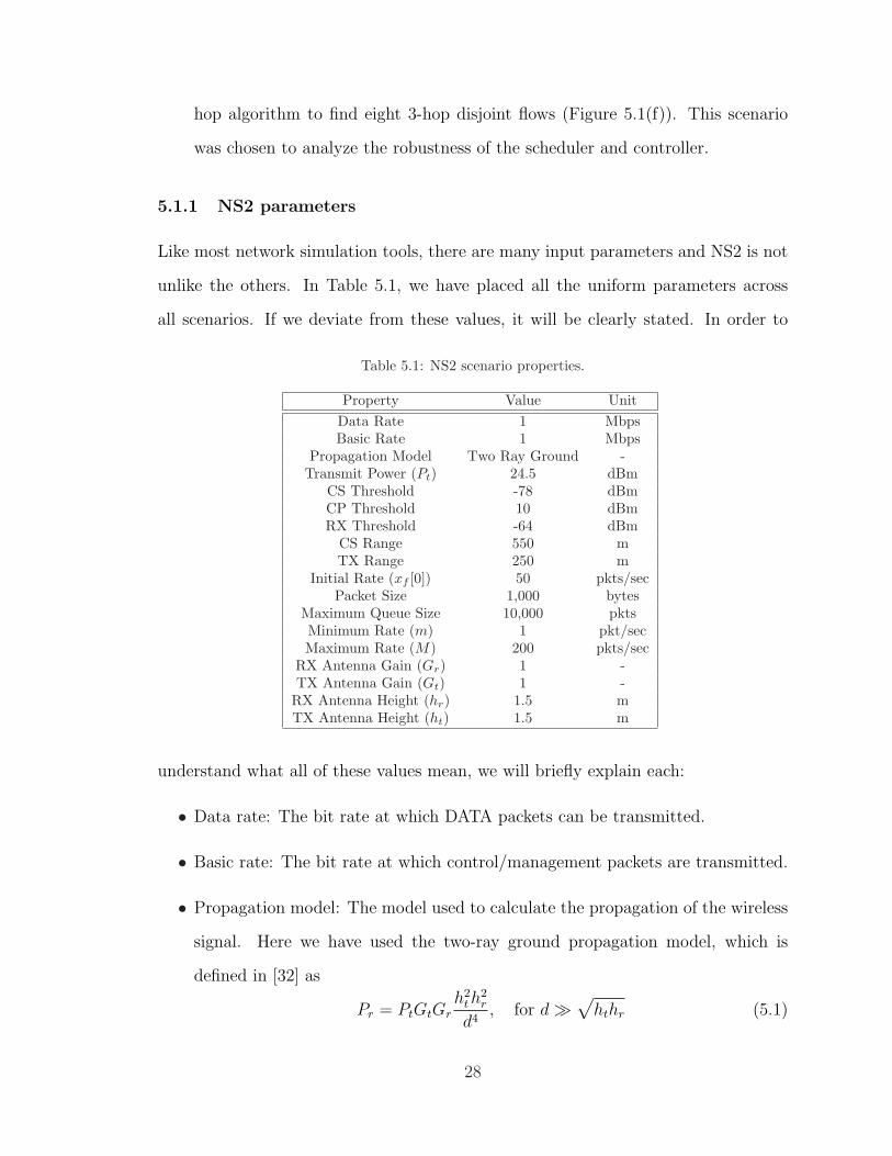
unlike the others. In Table 5.1, we have placed all the uniform parameters across

all scenarios. If we deviate from these values, it will be clearly stated. In order to

Table 5.1: NS2 scenario properties.

Property Value UnitData Rate 1 MbpsBasic Rate 1 Mbps

Propagation Model Two Ray Ground -Transmit Power (Pt) 24.5 dBm

CS Threshold -78 dBmCP Threshold 10 dBmRX Threshold -64 dBm

CS Range 550 mTX Range 250 m

Initial Rate (xf [0]) 50 pkts/secPacket Size 1,000 bytes

Maximum Queue Size 10,000 pktsMinimum Rate (m) 1 pkt/secMaximum Rate (M) 200 pkts/sec

RX Antenna Gain (Gr) 1 -TX Antenna Gain (Gt) 1 -RX Antenna Height (hr) 1.5 mTX Antenna Height (ht) 1.5 m

understand what all of these values mean, we will briefly explain each:

• Data rate: The bit rate at which DATA packets can be transmitted.

• Basic rate: The bit rate at which control/management packets are transmitted.

• Propagation model: The model used to calculate the propagation of the wireless

signal. Here we have used the two-ray ground propagation model, which is

defined in [32] as

Pr = PtGtGrh2

t h2r

d4, for d À

√hthr (5.1)

28

where Pr and Pt are the received and transmitted power, Gr and Gt are the

receiver and transmitter antenna gain constants, hr and ht are the height of the

receiver and transmitter antenna, and d is the distance between the transmitter

and receiver.

• CS threshold: If the received power is below the carrier sense (CS) threshold,

then the channel is deemed to be idle.

• CP threshold: Suppose a packet A arrives at node n with receive power Pr(A) at

t = 0 and is not done being received until t = 1. Now also assume that another

node transmits a packet B and it arrives at n at t = 0.5 with power Pr(B). Now,

NS2 compares the received powers to decide whether packet A will be correctly

received. The decision is made according to

10 log(Pr(A))− 10 log(Pr(B))no collision

≷collision

CPthresh, (5.2)

where CPthresh is the capture threshold in dBm.

• RX threshold: The receive threshold is the receive power threshold below which

a packet cannot be correctly decoded, or received.

• CS range: Given the transmit power and the carrier sense threshold, this is the

range at which a node can sense another node transmitting a packet.

• TX range: Given the transmit power and the receive threshold, and assuming

no interference, this is the range at which a node can correctly decode a packet.

• Initial rate: The initial CBR flow rate at the beginning of the simulation (at

t = 0).

• Packet size: The size of the DATA packets generated by the CBR module.

• Maximum queue size: The maximum size of the queue. If the queue overflows,

packets will be discarded.

29

• Minimum rate: The minimum flow rate of the congestion controller.

• Maximum rate: The maximum flow rate of the congestion controller.

5.2 Simulations

5.2.1 Symmetric local area network

In these scenarios, all nodes are within the transmission range of all other nodes.

Thus, only one node can transmit at a time without causing a collision. The 4-flow

and 8-flow scenario can be seen in Figure 5.1.

In this set of simulations, we want to see the following two things:

• The effect of changing the frequency of the backpressure broadcasts. We will

denote the backpressure broadcast frequency as

BPfreq =1

∆bp

, (5.3)

where ∆bp denotes the time, in seconds, between each broadcast of backpressure

information.

• The effect of using the two different congestion window update schemes in the

distributed scheduler, as explained in Section 4.3.

We would expect to see a unique optimal value of BPfreq, considering that too few

broadcasts would hurt the performance of the scheduler, but too many broadcast

packets will hurt overall throughput.

To gauge performance, we will look at the following metrics:

• Simulation average throughput: The CBR throughput averaged over the entire

simulation. In particular, we will compare this performance against the regular

802.11 throughput with each node always being backlogged. This will give us an

idea of the efficiency of the scheduler and the impact of the broadcast packets.

30

The simulation average throughput is calculated as

TPavg(0, T ) =1

T

∑

f∈Frfe(f)(0, T ), (5.4)

where T is the simulation time in seconds and rfn(t1, t2) represents the number

of packets from flow f received by node n in the interval [t1, t2].

• Average sum of utility: The goal of this system is to optimize the sum of the

utilities according to (3.5). This metric is calculated as

Uavgsum(Tstable, T ) =

1

|T |∑t∈T

∑

f∈FU(xf [t]), T = {Tstable, Tstable + 0.1, ..., T} ,

(5.5)

where Tstable is the point where the flow rates appear to begin to stabilize (de-

termined empirically) and T is the simulation time.

• Optimum sum of utility: This is the optimal sum of utility as seen in (4.12), given

that C equals the average throughput, TPavg(Tstable, T ), for that simulation.

In the 4-flow and 8-flow scenario the weights for the flows are βf = [1, 2, 3, 4]

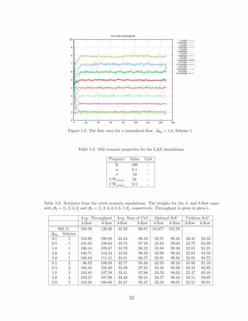
and βf = [1, 2, 3, 4, 5, 6, 7, 8] respectively. Figure 5.2 shows the normalized flow rates

with respect to time for one simulation. The flow rates are normalized with respect to

minf (x?f ), given that x?

f represents the optimal flow rate for flow f according to (4.10),

where C in this case is the average throughput in the simulation. For example, in the

4-flow 802.11 case, the average throughput is 108.59 pkts/s. Therefore, minf (x?f ) =

10.86 pkts/s.

In addition to Table 5.1, the parameters used in these simulations are given in

Table 5.2. The scenario statistics can be found in Tables 5.3 and 5.4. In the table,

we show the average throughput, average sum of utility, optimal sum of utility, and

the sum of utility if the flows were all uniform. The optimal sum term is calculated

using (4.12) where C is the average throughput in this case. The uniform sum term

31

0

1

2

3

4

5

6

7

8

9

10

0 20 40 60 80 100 120 140 160

Flow Rates (Normalized)

1 (calc)1 (actual)

3 (calc)3 (actual)

5 (calc)5 (actual)

7 (calc)7 (actual)

9 (calc)9 (actual)11 (calc)

11 (actual)13 (calc)

13 (actual)15 (calc)

15 (actual)

Figure 5.2: The flow rates for a normalized flow. ∆bp = 1.0, Scheme 1.

Table 5.2: NS2 scenario properties for the LAN simulations.

Property Value UnitK 100 -α 0.1 -σ 10 -

CWumin 31 -CWumax 511 -

Table 5.3: Statistics from the circle scenario simulations. The weights for the 4- and 8-flow caseswith βf = [1, 2, 3, 4] and βf = [1, 2, 3, 4, 5, 6, 7, 8], respectively. Throughput is given in pkts/s.

Avg. Throughput Avg. Sum of Util Optimal SoU Uniform SoU4-flow 8-flow 4-flow 8-flow 4-flow 8-flow 4-flow 8-flow

802.11 108.59 120.46 32.92 96.87 34.077 102.76∆bp Scheme0.1 1 102.60 106.89 33.43 96.10 33.51 98.46 32.45 93.320.5 1 105.94 108.60 33.74 97.76 33.83 99.03 32.77 93.891.0 1 106.44 109.67 33.79 98.22 33.88 99.38 32.81 94.252.0 1 106.71 110.44 33.82 98.43 33.90 99.63 32.84 94.505.0 1 106.83 111.15 33.81 98.57 33.91 99.86 32.85 94.730.1 2 96.82 100.50 32.77 94.49 32.93 96.24 31.86 91.100.5 2 102.34 105.80 33.39 97.35 33.48 98.09 32.42 92.951.0 2 102.85 107.38 33.41 97.96 33.53 98.62 32.47 93.492.0 2 103.27 107.99 33.48 98.24 33.57 98.83 32.51 93.695.0 2 103.28 108.66 33.47 98.47 33.58 99.05 32.51 93.91

32

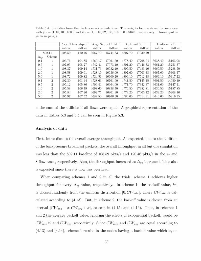
Table 5.4: Statistics from the circle scenario simulations. The weights for the 4- and 8-flow caseswith βf = [1, 10, 100, 1000] and βf = [1, 3, 10, 32, 100, 316, 1000, 3162], respectively. Throughput isgiven in pkts/s.

Avg. Throughput Avg. Sum of Util Optimal SoU Uniform SoU4-flow 8-flow 4-flow 8-flow 4-flow 8-flow 4-flow 8-flow

802.11 108.59 120.46 3667.70 15744.83 4807.70 17939.79∆bp Scheme0.1 1 105.76 104.85 4760.17 17091.60 4778.40 17298.04 3638.40 15103.080.5 1 107.95 108.27 4742.41 17073.40 4801.20 17446.33 3661.20 15251.371.0 1 108.37 109.14 4731.73 16982.40 4805.50 17483.46 3665.50 15288.502.0 1 108.58 109.61 4728.19 16936.00 4807.60 17503.33 3667.60 15308.375.0 1 108.72 109.82 4724.56 16900.20 4809.10 17512.18 3669.10 15317.220.1 2 102.30 101.44 4728.66 16761.60 4741.50 17145.15 3601.50 14950.190.5 2 105.12 105.86 4709.41 16964.00 4771.70 17342.37 3631.60 15147.411.0 2 105.58 106.79 4698.60 16858.70 4776.50 17382.81 3636.50 15187.852.0 2 105.84 107.26 4692.75 16801.90 4779.20 17403.12 3639.20 15208.165.0 2 105.97 107.52 4689.50 16766.30 4780.60 17414.31 3640.60 15219.35

is the sum of the utilities if all flows were equal. A graphical representation of the

data in Tables 5.3 and 5.4 can be seen in Figure 5.3.

Analysis of data

First, let us discuss the overall average throughput. As expected, due to the addition

of the backpressure broadcast packets, the overall throughput in all but one simulation

was less than the 802.11 baseline of 108.59 pkts/s and 120.46 pkts/s in the 4- and

8-flow cases, respectively. Also, the throughput increased as ∆bp increased. This also

is expected since there is now less overhead.

When comparing schemes 1 and 2 in all the trials, scheme 1 achieves higher

throughput for every ∆bp value, respectively. In scheme 1, the backoff value, bv,

is chosen randomly from the uniform distribution [0, CWmin], where CWmin is cal-

culated according to (4.13). But, in scheme 2, the backoff value is chosen from an

interval [CWavg − σ,CWavg + σ], as seen in (4.15) and (4.16). Thus, in schemes 1

and 2 the average backoff value, ignoring the effects of exponential backoff, would be

CWmin/2 and CWavg, respectively. Since CWmin and CWavg are equal according to

(4.13) and (4.14), scheme 1 results in the nodes having a backoff value which is, on

33

31.5

32

32.5

33

33.5

34

34.5

0.1 0.1 0.5 0.5 1.0 1.0 2.0 2.0 5.0 5.0

Scheme 1Scheme 2

802.11

(a)

91

92

93

94

95

96

97

98

99

100

0.1 0.1 0.5 0.5 1.0 1.0 2.0 2.0 5.0 5.0

Scheme 1Scheme 2

802.11

(b)

3400

3600

3800

4000

4200

4400

4600

4800

5000

0.1 0.1 0.5 0.5 1.0 1.0 2.0 2.0 5.0 5.0

Scheme 1Scheme 2

802.11

(c)

15000

15500

16000

16500

17000

17500

0.1 0.1 0.5 0.5 1.0 1.0 2.0 2.0 5.0 5.0

Scheme 1Scheme 2

802.11

(d)

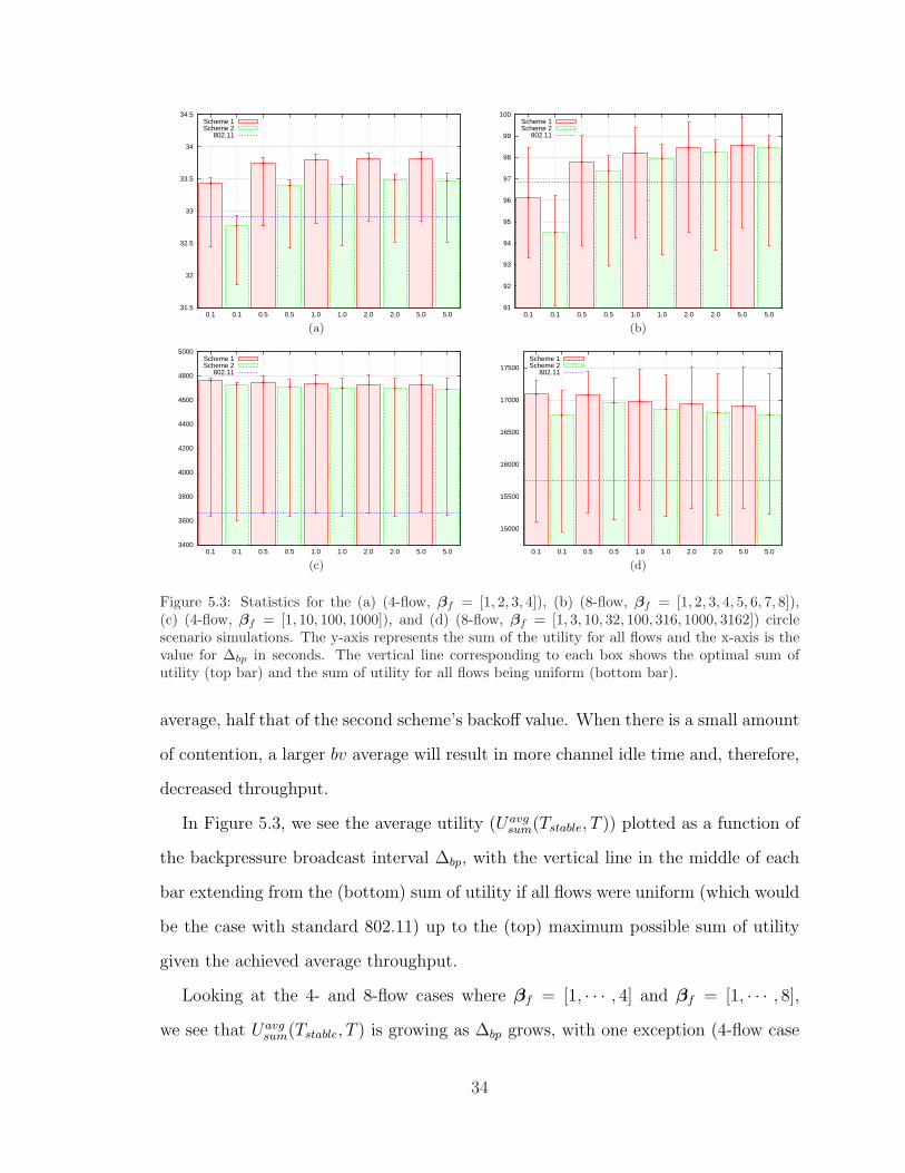
Figure 5.3: Statistics for the (a) (4-flow, βf = [1, 2, 3, 4]), (b) (8-flow, βf = [1, 2, 3, 4, 5, 6, 7, 8]),(c) (4-flow, βf = [1, 10, 100, 1000]), and (d) (8-flow, βf = [1, 3, 10, 32, 100, 316, 1000, 3162]) circlescenario simulations. The y-axis represents the sum of the utility for all flows and the x-axis is thevalue for ∆bp in seconds. The vertical line corresponding to each box shows the optimal sum ofutility (top bar) and the sum of utility for all flows being uniform (bottom bar).

average, half that of the second scheme’s backoff value. When there is a small amount

of contention, a larger bv average will result in more channel idle time and, therefore,

decreased throughput.

In Figure 5.3, we see the average utility (Uavgsum(Tstable, T )) plotted as a function of

the backpressure broadcast interval ∆bp, with the vertical line in the middle of each

bar extending from the (bottom) sum of utility if all flows were uniform (which would

be the case with standard 802.11) up to the (top) maximum possible sum of utility

given the achieved average throughput.

Looking at the 4- and 8-flow cases where βf = [1, · · · , 4] and βf = [1, · · · , 8],

we see that Uavgsum(Tstable, T ) is growing as ∆bp grows, with one exception (4-flow case

34

where ∆bp increases from 2.0 to 5.0). This steady growth is due to the throughput

increase coupled with the fact that the large broadcast interval does not hurt much in

this scenario because it is a single hop route, the traffic is constant, and the scenario

is symmetric. Looking at the vertical lines in the 8-flow scenario, we see that scheme

2 is higher to the maximum achievable, but scheme 1 still outperforms due to the

higher throughput. That is, scheme 2 may provide a better system to correctly assign

priority, but it loses in the long run due to its poor throughput when compared to

scheme 1. In the 4-flow scenarios, scheme 1 with ∆bp = 2.0 performed the best. In

the 8-flow scenarios, scheme 1 with ∆bp = 5.0 performed the best.

Looking at the 4- and 8-flow cases where βf = [1, · · · , 1000] and βf = [1, · · · , 3162],

we see that Uavgsum(Tstable, T ) is decreasing as ∆bp increases, with one exception (8-flow

case using scheme 1 where ∆bp increases from 0.1 to 0.5). However, in all of these

cases, the average throughput increases as ∆bp increases. So, we see here that the

weights make a larger difference. Because these weights are growing exponentially, it

is much more important (when compared to the linear weight growth) for the flows

to reach the fair rate allocation point, specifically the flows with large weights. In

order to reach fair rate allocation, the nodes need up-to-date backpressure information

which can be achieved by more broadcast messages (i.e., a low ∆bp). Thus, in these

cases, the lower ∆bp values correspond to the best Uavgsum(Tstable, T ) values. In both the

4- and 8-flow scenarios, scheme 1 with ∆bp = 0.1 performed the best.

In both weighting schemes, we observe that the achieved Uavgsum(Tstable, T ) is closer

to the maximum possible sum of utility in the 4-flow case than the 8-flow case. This is

due to the increased contention and imperfect backpressure information. As the num-

ber of competing flows increases, the number of broadcast messages increases in the

contention region and collisions happen and less accurate backpressure information

is used by the scheduler, adversely effecting performance.

In Figure 5.3, we have plotted Uavgsum(Tstable, T ) for the standard 802.11 case (i.e.,

no utility-based scheduler or congestion controller) shown by the blue dashed line.

35

In the linear weighting scheme, we see that the 802.11 case actually performs better

than a few of the cases which use the utility-based scheduler and congestion controller.

However, this does not happen, or even come close to happening, with the exponential

weighting setup. This is because the optimal flows, x?f , are spread out linearly for

the linear weighting scheme and exponentially for the exponential weighting scheme.

So, if the flows’ throughputs are uniform, then it will have a worse effect on the

exponential weighting scheme. One can extend this result to say that utility-based

scheduling and congestion control is more effective when the weighting scheme is

more diverse or spread out. Due to the limited scope of this thesis, we will limit the

following two scenarios to the linear weighting scheme.

5.2.2 Multihop multiflow straight line

In the straight line simulations, we want to see how the system works when nodes are

forwarding multiple flows. The 8-flow scenario layout can be seen in Figure 5.1(d),

with the transmission ranges and carrier sense range shown in Figure 5.1(c). In this

scenario, the forwarding nodes (n10, n9, n8) have to forward the traffic for all flows,

which all have different destinations. For example, the second flow is generated by

n12 and is destined for n1 via the route n12 → n10 → n9 → n8 → n1. At the start of

the simulation, all the nodes at x = 200 m begin transmitting packets destined for

the nodes at x = 1000 m.

Also, unlike the circular LAN scenarios, these scenarios allow for simultaneous

transmissions. The transmission and carrier sense ranges are set to 250 and 550 m,

respectively. This can be seen clearly in Figure 5.1(c). This setup allows a node at

x = 200 to transmit while a node at x = 800 also transmits. The following are the

combinations where simultaneous transmission could occur (the numbers represent

the set of nodes by their x-coordinate): [200,800], [200,1000], and [400,1000].

36

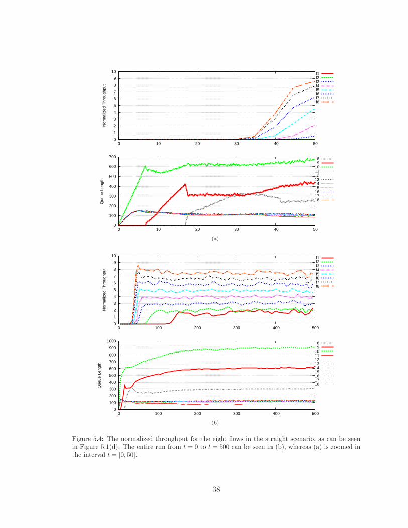
Analysis of data

Before we discuss any throughput or utility results, let us first discuss what is hap-

pening in Figure 5.4. The figure shows the normalized instantaneous throughput and

the overall queue size for all 8 flows for one scenario, with t ranging from 0 to 50 in

(a) and 0 to 500 in (b). The throughput is normalized with respect to minf∈F{x?f},

where x?f is the optimal fair rate for flow f given in (3.5) and can be calculated, in this

case, using (4.11). Since the weights used are βf = [1, 2, 3, 4, 5, 6, 7, 8], the normalized

optimal rates are also [1, 2, 3, 4, 5, 6, 7, 8].

In (b), we see that the scheduler/controller is doing a pretty good job of getting

the rates to their fair rate allocation point, with the exception of flows f1, f7, and

f8. Flow f1 is almost twice its optimal and flows f7 and f8 are below their optimal

points. Flows f2-f6 are all oscillating right around their optimal points.

Recall that the queues-per-destination and the overall queue will be abbreviated

as QPFs and OQ, respectively, where the overall queue is the sum of all the QPFs at

a given node.

In (a), we see the normalized throughput and the overall queue length, OQ, from

t = 0 to t = 50 s. We will start from t = 0 and explain what is happening. At t = 0

the simulation begins and nodes n11 through n18 begin generating packets at a rate

of 50 pkts/s, per the NS2 scenario properties given in Table 5.1. These packets are

destined for nodes at x = 1000 and must go through the path n10 → n9 → n8. Since

n10 is the next hop for all 8 flows, n10 begins to get a lot of packets and its QPFs

grow quickly, as shown by the growth in the OQ. In the meantime, the QPFs at the

generating nodes also grow because the channel cannot withstand a rate of 50 × 8

pkts/s. Between t = 0 and t = 6, due to the backpressure scheduler, n10’s OQ grows

linearly and n9’s OQ stays empty. This is because all of the nodes at x = 200 have

higher backpressure values than n10; therefore, n10 has a high backoff value and a

low priority to access the channel, resulting in very few packets reaching n9 during

37

0

1

2

3

4

5

6

7

8

9

10

0 10 20 30 40 50

Nor

mal

ized

Thr

ough

put

f1f2f3f4f5f6f7f8

0

100

200

300

400

500

600

700

0 10 20 30 40 50

Que

ue L

engt

h

89

101112131415161718

(a)

0

1

2

3

4

5

6

7

8

9

10

0 100 200 300 400 500

Nor

mal

ized

Thr

ough

put

f1f2f3f4f5f6f7f8

0

100

200

300

400

500

600

700

800

900

1000

0 100 200 300 400 500

Que

ue L

engt

h

89

101112131415161718

(b)

Figure 5.4: The normalized throughput for the eight flows in the straight scenario, as can be seenin Figure 5.1(d). The entire run from t = 0 to t = 500 can be seen in (b), whereas (a) is zoomed inthe interval t = [0, 50].

38

this time period. At t = 6, this changes and the backpressure values (one for each

destination n0-n7) at n10 are now comparable to those at n11-n18. Thus, n10 begins to

gain access to the channel and forwards packets to n9. From t = 6 until t = 17, the

same thing that happened at n10 during t = [0, 6] happens at n9. That is, the QPFs

have to build up at n9 before the backpressure values are large enough to gain a high

priority to access the channel. At t = 17, n9’s QPFs have grown sufficiently large and

can now forward packets to n8. From t = 17 to t = 31, n8’s QPFs grow until it can

forward traffic to the end destinations. At t = 31, we start to see packets arriving

at the end destinations. However, in (b) we see that some flows do not start getting

packets to their destinations until much later. Namely, f2 and f1 do not start getting

meaningful throughput until around t = 70 and t = 125, respectively. This is due to

the fact that the lower priority flows have a harder time getting packets forwarded

initially due to their low priority.

In Table 5.5, we see the average throughput and the sum of utility, broken up

by three time intervals, for several simulations. It is broken up into time intervals

due to the large delay in forwarding of packets as can be seen in Figure 5.4. To

use as comparison, the link capacity is 125 pkts/s, considering a packet size of 1000

bytes and a physical rate of 1 Mbps. Considering the interference region and taking

advantage of spatial reuse, the throughput capacity is given by 1253

, or 41.67 pkts/s.

In the first row we have the 802.11 baseline statistics. The 802.11 scenario was

hampered by a lot of collisions which led to poor throughout. As expected, it grew

a little, but was fairly uniform throughout each interval. Due to the low throughput

and the uniformity in flows, the utility term was very low.

For both schemes, we varied the α and K congestion controller parameters in order

to see their effect on this scenario. As stated earlier, α controls the rate of change of

the flow rate. The larger α is, the faster the flow rate changes. We also tested against

the two schemes and the broadcast interval, ∆bp. In average throughput, scheme 1 had

the maximum value in all three intervals, and also over the whole interval of [0,150],

39

Table 5.5: Performance of the multihop multiflow straight line simulations. Note: In calculatingUavg

sum(·, ·), if xf [t] = 0 for some t, we would use xf [t] = 0.01 instead due to ln(0) = −∞.

TPavg(x, y) Uavgsum(x, y)

α K ∆bp 0,50 50,100 100,150 0,150 0,50 50,100 100,150802.11 17.76 18.8 19.7551 18.7651 26.7141 27.111 26.4652

Scheme 10.1 100 0.1 22.58 25.86 29.55 25.97 31.82 43.11 50.320.1 100 0.5 24.88 27.12 30.35 27.43 39.17 47.44 50.240.1 100 1.0 24.70 28.50 28.84 27.34 41.64 47.44 46.690.1 500 0.1 14.00 24.96 27.10 21.99 -22.45 24.02 26.660.1 500 0.5 16.06 26.98 28.08 23.68 -32.03 21.08 27.840.1 500 1.0 16.36 26.62 27.61 23.50 -9.36 27.66 32.77

0.01 100 0.1 17.80 28.68 30.98 25.78 7.91 49.57 52.610.01 100 0.5 19.60 29.04 31.10 26.55 26.29 49.23 49.950.01 100 1.0 21.00 27.98 30.06 26.32 35.40 46.74 48.250.01 500 0.1 13.40 26.66 26.26 22.08 -16.18 28.16 32.440.01 500 0.5 15.26 28.06 28.45 23.89 -5.41 31.66 34.960.01 500 1.0 15.00 27.28 28.61 23.60 -34.44 28.06 39.13

Scheme 20.1 100 0.1 8.52 25.76 28.18 20.77 -47.88 36.92 40.580.1 100 0.5 11.56 26.10 29.06 22.19 -40.08 41.69 47.780.1 100 1.0 15.66 27.08 28.69 23.78 -4.89 44.19 45.960.1 500 0.1 6.96 20.56 19.33 15.59 -32.78 18.55 18.990.1 500 0.5 13.36 23.18 21.75 19.41 -6.16 23.19 22.710.1 500 1.0 15.22 23.68 22.49 20.45 2.62 23.62 23.63

0.01 100 0.1 4.10 27.06 28.57 19.85 -120.36 41.60 47.130.01 100 0.5 15.44 27.70 30.12 24.38 7.81 45.27 48.550.01 100 1.0 15.70 27.72 29.41 24.24 14.85 45.72 46.510.01 500 0.1 3.92 18.90 17.88 13.54 -46.04 17.37 19.810.01 500 0.5 12.32 21.72 20.86 18.28 -10.31 22.33 22.910.01 500 1.0 13.12 22.42 22.06 19.18 -11.01 25.66 28.07

as shown by the numbers in bold. Surprisingly, in scheme 1, ∆bp = 0.5 provided

the maximum throughput in [0,150] for all values of α and K, when compared to

∆bp = 0.1 and ∆bp = 1.0. In scheme 2, ∆bp = 1.0 provided the maximum in three

out of the four α,K combinations. Also, notice that in both schemes, the K = 100

trials achieved more throughput than the K = 500 trials because the higher the

K value is, then the higher the queue must be in order to drive ∆xfto 0. If the

queue has to be larger, then it will take longer for the backpressure values at n10-

n8 to level out and get the first packet of each flow to its destinations. Over the

whole interval [0,150], the maximum average throughput was achieved by scheme 1

using parameters [α,K, ∆bp] = [0.1, 100, 0.5]. As for the average of the sum utility,

40

Uavgsum, scheme 1 also had the maximum value for all three intervals. With [α, K]

being constant, Uavgsum(0, 50) increased with ∆bp because more packets were making

it to the destination faster due to innacurate (old) backpressure information at the

intermediate nodes. With only 1 broadcast packet every second, the intermediate

nodes would think that their backpressure was large enough to have priority access

to the channel. However, for the other two intervals, the lower ∆bp values proved

better due to more accurate backpressure information. For the last two intervals,

scheme 1 with parameters [α,K, ∆bp] = [0.01, 100, 0.1] achieved the highest Uavgsum,

with Uavgsum(50, 100) = 49.57 and Uavg

sum(100, 150) = 52.61. These parameters will be

used in the random scenarios. For that case and with C = 30.98, the optimal sum is

53.88 and the sum with uniform flows is 48.74.

5.2.3 Random topology

In the random topology trials, we generated scenarios with eight three-hop disjoint

flows. That is, every node only forwards traffic for, at most, one node. To generate

the scenarios, we first randomly placed nodes on a 1000 m x 1000 m grid. Then, for

each of the eight flows, we selected a random source node and a random destination

node. Using Dijktra’s shortest route algorithm, a route was selected. If the route was

three hops long and did not contain any nodes from any of the other flows, then it

was added. Twenty of these scenarios were generated. A sample scenario is shown in

Figure 5.1(f).

For the sake of brevity, we decided it was only necessary to run the random tests

across one set of parameters. A good performing set of parameters from the straight-

line simulations were used and can be seen in Table 5.6.

Table 5.7 shows the average throughput across all random scenarios, both for the

case where the scheduler/controller was used and also for the simple 802.11 case. It

is also broken down into time intervals for analyzing.

41

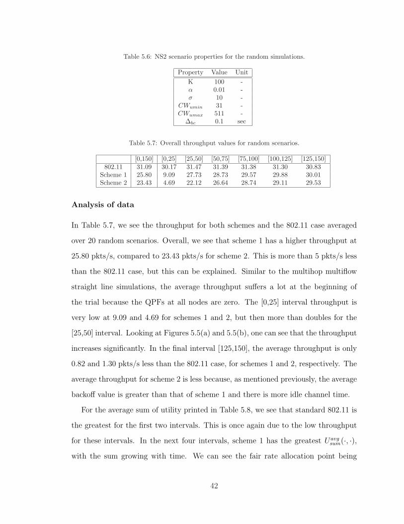
Table 5.6: NS2 scenario properties for the random simulations.

Property Value UnitK 100 -α 0.01 -σ 10 -

CWumin 31 -CWumax 511 -

∆bc 0.1 sec

Table 5.7: Overall throughput values for random scenarios.

[0,150] [0,25] [25,50] [50,75] [75,100] [100,125] [125,150]802.11 31.09 30.17 31.47 31.39 31.38 31.30 30.83

Scheme 1 25.80 9.09 27.73 28.73 29.57 29.88 30.01Scheme 2 23.43 4.69 22.12 26.64 28.74 29.11 29.53

Analysis of data

In Table 5.7, we see the throughput for both schemes and the 802.11 case averaged

over 20 random scenarios. Overall, we see that scheme 1 has a higher throughput at

25.80 pkts/s, compared to 23.43 pkts/s for scheme 2. This is more than 5 pkts/s less

than the 802.11 case, but this can be explained. Similar to the multihop multiflow

straight line simulations, the average throughput suffers a lot at the beginning of

the trial because the QPFs at all nodes are zero. The [0,25] interval throughput is

very low at 9.09 and 4.69 for schemes 1 and 2, but then more than doubles for the

[25,50] interval. Looking at Figures 5.5(a) and 5.5(b), one can see that the throughput

increases significantly. In the final interval [125,150], the average throughput is only

0.82 and 1.30 pkts/s less than the 802.11 case, for schemes 1 and 2, respectively. The

average throughput for scheme 2 is less because, as mentioned previously, the average

backoff value is greater than that of scheme 1 and there is more idle channel time.

For the average sum of utility printed in Table 5.8, we see that standard 802.11 is

the greatest for the first two intervals. This is once again due to the low throughput

for these intervals. In the next four intervals, scheme 1 has the greatest Uavgsum(·, ·),

with the sum growing with time. We can see the fair rate allocation point being

42

0

1

2

3

4

5

6

7

1 2 3 4 5 6 7 8

Thr

ough

put (

pkts

/sec

)

Flow ID

Scheme 1Scheme 2

(a)

0

1

2

3

4

5

6

7

1 2 3 4 5 6 7 8

Thr

ough

put (

pkts

/sec

)

Flow ID

Scheme 1Scheme 2

(b)

0

1

2

3

4

5

6

7

1 2 3 4 5 6 7 8

Thr

ough

put (

pkts

/sec

)

Flow ID

Scheme 1Scheme 2

(c)

0

1

2

3

4

5

6

7

1 2 3 4 5 6 7 8

Thr

ough

put (

pkts

/sec

)

Flow ID

Scheme 1Scheme 2

(d)

0

1

2

3

4

5

6

7

1 2 3 4 5 6 7 8

Thr

ough

put (

pkts

/sec

)

Flow ID

Scheme 1Scheme 2

(e)

0

1

2

3

4

5

6

7

1 2 3 4 5 6 7 8

Thr

ough

put (

pkts

/sec

)

Flow ID

Scheme 1Scheme 2

(f)

Figure 5.5: Throughput of the flows in the random scenarios. The throughput was averaged acrossall 20 runs and the error bar shows the standard deviation of each flow. The plots are for timeintervals (a) [0:25], (b) [25:50], (c) [50:75], (d) [75,100], (e) [100,125], and (f) [125,150] seconds.

43

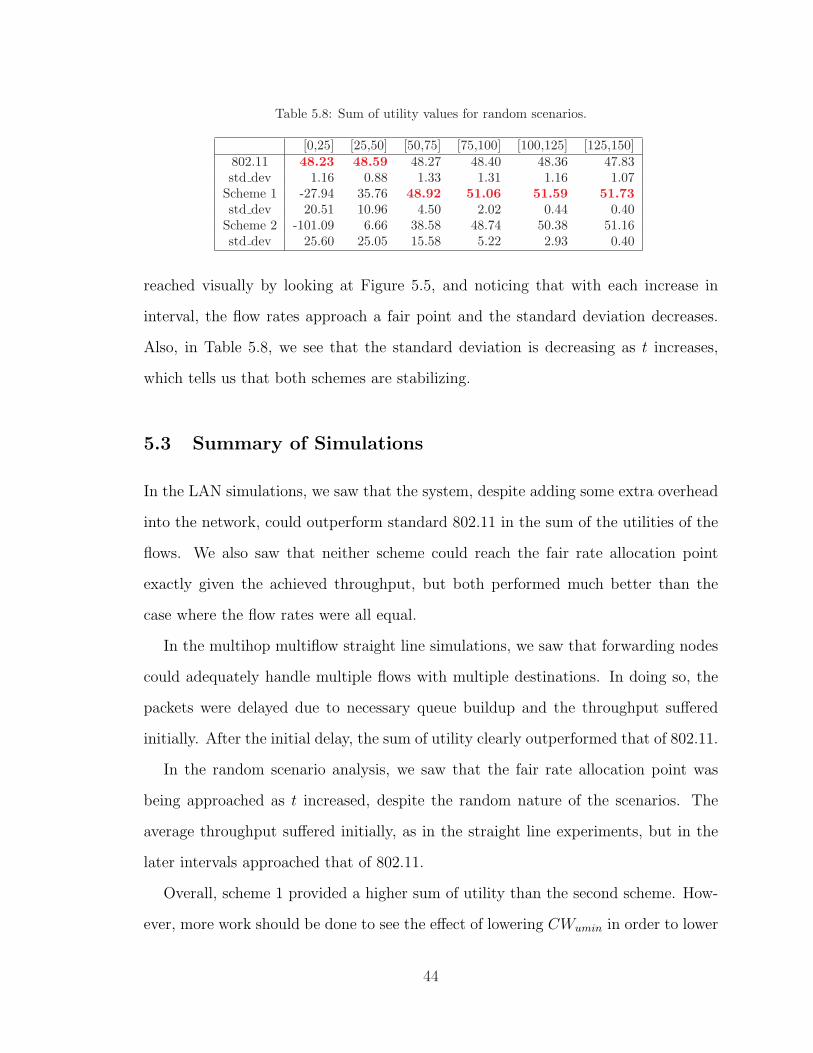
Table 5.8: Sum of utility values for random scenarios.

[0,25] [25,50] [50,75] [75,100] [100,125] [125,150]802.11 48.23 48.59 48.27 48.40 48.36 47.83std dev 1.16 0.88 1.33 1.31 1.16 1.07

Scheme 1 -27.94 35.76 48.92 51.06 51.59 51.73std dev 20.51 10.96 4.50 2.02 0.44 0.40

Scheme 2 -101.09 6.66 38.58 48.74 50.38 51.16std dev 25.60 25.05 15.58 5.22 2.93 0.40

reached visually by looking at Figure 5.5, and noticing that with each increase in

interval, the flow rates approach a fair point and the standard deviation decreases.

Also, in Table 5.8, we see that the standard deviation is decreasing as t increases,

which tells us that both schemes are stabilizing.

5.3 Summary of Simulations

In the LAN simulations, we saw that the system, despite adding some extra overhead

into the network, could outperform standard 802.11 in the sum of the utilities of the

flows. We also saw that neither scheme could reach the fair rate allocation point

exactly given the achieved throughput, but both performed much better than the

case where the flow rates were all equal.

In the multihop multiflow straight line simulations, we saw that forwarding nodes

could adequately handle multiple flows with multiple destinations. In doing so, the

packets were delayed due to necessary queue buildup and the throughput suffered

initially. After the initial delay, the sum of utility clearly outperformed that of 802.11.

In the random scenario analysis, we saw that the fair rate allocation point was

being approached as t increased, despite the random nature of the scenarios. The

average throughput suffered initially, as in the straight line experiments, but in the

later intervals approached that of 802.11.

Overall, scheme 1 provided a higher sum of utility than the second scheme. How-

ever, more work should be done to see the effect of lowering CWumin in order to lower

44

the average backoff value for the second scheme. As far as the backpressure broadcast,

ten per second (∆bp = 0.1) seemed to work the best in multihop situations, whereas

one every two seconds seemed adequate for the LAN one-hop scenario.

45

CHAPTER 6

CONCLUSIONS AND FUTURE WORK

In this thesis, we propose a distributed backpressure-based congestion controller and

scheduler system, based upon the controller-scheduler described in [1]. This system

allows for flows within a wireless network to be assigned a weighted utility that is a

function of the flow rate. The goal of the system is to maximize the sum of all of the

utilities of all the flows in the network, as seen in (3.5).

In our simulations, we showed that while the flow rates did not converge to the

optimal solution, they did converge very closely at times and almost always performed

better than standard 802.11. Our simulations highlighted the performance of this

distributed system in three topologies: a simple LAN, a fixed multihop scenario,

and a random multihop scenario. We also compared two different schemes for the

backpressure-based scheduler.

We believe that, although a lot was learned through the work performed in this

thesis, there is still more work that needs to be done. Thus, we would like to propose

some future work. The following list highlights some of the areas/ideas that we would

like to pursue to extend this distributed controller-scheduler in attempt to establish

a solid framework:

• Physical layer rate control: Instead of controlling the flow rate at the MAC layer,

one could harness the power of the physical layer rate control.

• Move the broadcast packets down to the MAC layer: Currently, mainly due

to simulation ease, the broadcast packets come from the application layer even

though they should be generated by the MAC layer. In future simulations, we

46

should move all of the scheduler components down to the MAC layer.

• Evaluate non-802.11 based system: In our simulations, we took the standard

802.11 MAC and physical layer and modified it to incorporate our scheduler and

controller. It would be valuable to look at a clean slate approach and not restrict

oneself to the confines of the 802.11 standard.

47

REFERENCES

[1] A. Eryilmaz and R. Srikant, “Joint congestion control, routing, and MAC forstability and fairness in wireless networks,” IEEE Journal on Selected Areas inCommunications, vol. 24, no. 8, pp. 1514–1524, 2006.

[2] The network simulator—ns-2. [Online]. Available: http://www.isi.edu/nsnam/ns/.

[3] M. S. Gast, 802.11 Wireless Networks: The Definitive Guide, M. Loukides, Ed.Sebastopol, CA: O’Reilly & Associates, Inc., 2002.

[4] LAN/MAN Standards Committee of the IEEE Computer Society.ANSI/IEEE Std 802.11, 1999 Edition (R2003). [Online]. Available:http://standards.ieee.org/getieee802/802.11.html.

[5] J. Deng and R.-S. Chang, “A priority scheme for IEEE 802.11 DCF accessmethod,” IEICE Transactions on Communication, vol. E82-B, no. 1, pp. 96–102, 1999.

[6] Y. Xiao, “A simple and effective priority scheme for IEEE 802.11,” IEEE Com-munication Letters, vol. 7, no. 2, pp. 70–72, 2003.

[7] N. Vaidya, A. Dugar, S. Gupta, and P. Bahl, “Distributed fair scheduling ina wireless LAN,” IEEE Transactions on Mobile Computing, vol. 4, no. 6, pp.616–629, 2005.

[8] L. Tassiulas and A. Ephremides, “Stability properties of constrained queueingsystems and scheduling policies for maximum throughput in multihop radio net-works,” IEEE Transactions on Automatic Control, vol. 37, no. 12, pp. 1936–1948,1992.

[9] H. Yaiche, R. R. Mazumdar, and C. Rosenberg, “A game-theoretic framework forbandwidth allocation and pricing in broadband networks,” IEEE/ACM Trans-actions on Networking, vol. 8, no. 5, pp. 667–678, 2000.

[10] S. Kunniyur and R. Srikant, “A time-scale decomposition approach to adaptiveECN marking,” IEEE Transactions on Automatic Control, vol. 47, no. 6, pp.882–894, 2002.

[11] T. Alpcan and T. Basar, “A utility-based congestion control scheme for internet-style networks with delay,” in Proceedings of IEEE INFOCOM, San Francisco,CA, March 2003, pp. 2039–2048.

48

[12] F. P. Kelly, A. Maulloo, and D. Tan, “Rate control in communication networks:Shadow prices, proportional fairness and stability,” Journal of the OperationalResearch Society, vol. 49, no. 3, pp. 237–252, 1998.

[13] S. H. Low and D. E. Lapsley, “Optimization flow control, I: Basic algorithmand convergence,” IEEE/ACM Transactions on Networking, vol. 7, no. 6, pp.861–874, 1999.

[14] J. T. Wen and M. Arcak, “A unifying passivity framework for network flowcontrol,” IEEE Transactions on Automatic Control, vol. 49, no. 2, pp. 162–174,2004.

[15] A. Eryilmaz and R. Srikant, “Fair resource allocation in wireless networks usingqueue-length based scheduling and congestion control,” in Proceedings of IEEEINFOCOM, Miami, FL, March 2005, pp. 1794–1803.

[16] L. Chen, S. H. Low, and J. C. Doyle, “Joint congestion control and media accesscontrol design for wireless ad hoc networks,” in Proceedings of IEEE INFOCOM,Miami, FL, March 2005, pp. 2212–2222.

[17] X. Lin and N. Shroff, “The impact of imperfect scheduling on cross-layer rate con-trol in multihop wireless networks,” in Proceedings of IEEE INFOCOM, Miami,FL, March 2005, pp. 1804–1814.

[18] Y. Yi and S. Shakkottai, “Hop-by-hop congestion control over a wireless multi-hop network,” in Proceedings of IEEE INFOCOM, Hong Kong, March 2004, pp.2548–2558.

[19] M. Chiang, “To layer or not to layer: Balancing transport and physical layersin wireless multihop networks,” in Proceedings of IEEE INFOCOM, Hong Kong,March 2004, pp. 2525–2536.

[20] L. Chen, S. H. Low, M. Chiang, and J. C. Doyle, “Cross-layer congestion control,routing and scheduling design in ad hoc wireless networks,” in Proceedings ofIEEE INFOCOM, Barcelona, Spain, April 2006, pp. 1–13.

[21] X. Lin and N. Shroff, “Joint rate control and scheduling in multihop wirelessnetworks,” in Proceedings of the IEEE Conference on Decision and Control, Par-adise Island, Bahamas, Dec. 2004, pp. 1484–1489.

[22] A. Stolyar, “Maximizing queueing network utility subject to stability: Greedyprimal-dual algorithm,” Queuing Systems, vol. 50, no. 4, pp. 401–457, 2005.

[23] M. J. Neely, E. Modiano, and C. Li, “Fairness and optimal stochastic control forheterogeneous networks,” in Proceedings of IEEE INFOCOM, Miami, FL, March2005, pp. 1723–1734.

[24] L. Tassiulas and S. Sarkar, “Maxmin fair scheduling in wireless networks,” inProceedings of IEEE INFOCOM, New York, NY, June 2002, pp. 763–772.

49

[25] X. Wu and R. Srikant, “Regulated maximal matching: A distributed schedulingalgorithm for multi-hop wireless networks with node-exclusive spectrum sharing,”in Proceedings of the IEEE Conference on Decision and Control, Seville, Spain,Dec. 2005, pp. 5342–5347.

[26] L. Bui, A. Eryilmaz, R. Srikant, and X. Wu, “Joint asynchronous congestioncontrol and distributed scheduling for wireless networks,” in Proceedings of IEEEINFOCOM, Barcelona, Spain, April 2006, pp. 1–12.

[27] P. Chaporkar, K. Kar, and S. Sarkar, “Throughput guarantees through maximalscheduling in wireless networks,” in Proceedings of the Allerton Conference onCommunication, Control, and Computing, Urbana, IL, Sept. 2005, pp. 1557–1567.

[28] X. Wu and R. Srikant, “Scheduling efficiency of distributed greedy schedulingalgorithms in wireless networks,” in Proceedings of IEEE INFOCOM, Barcelona,Spain, April 2006, pp. 1–12.

[29] J. Mo and J. Walrand, “Fair end-to-end window-based congestion control,”IEEE/ACM Transactions on Networking, vol. 8, no. 5, pp. 556–567, 2000.

[30] K. Fall and K. Varadhan, “The ns manual,” 2007. [Online]. Available:http://www.isi.edu/nsnam/ns/ns-documentation.html.

[31] “NS-MIRACLE: Multi-interface cross-layer extension library for the net-work simulator,” 2007. [Online]. Available: http://www.dei.unipd.it/wdyn/?IDsezione=3966.

[32] T. S. Rappaport, Wireless Communications: Principles and Practice. UpperSaddle River, NJ: Prentice Hall PTR, 2002.

50