by venkata krishna rao m - globaljournals.org filespectral kurtosis theory: a review through...

© 2015. Venkata Krishna Rao M. This is a research/review paper, distributed under the terms of the Creative Commons Attribution-Noncommercial 3.0 Unported License http://creativecommons.org/licenses/by-nc/3.0/), permitting all non commercial use, distribution, and reproduction in any medium, provided the original work is properly cited.

Global Journal of Researches in Engineering : F Electrical and Electronics Engineering Volume 15 Issue 6 Version 1.0 Year 2015 Type: Double Blind Peer Reviewed International Research Journal Publisher: Global Journals Inc. (USA) Online ISSN: 2249-4596 & Print ISSN: 0975-5861

Spectral Kurtosis Theory: A Review through Simulations

By Venkata Krishna Rao M Vidya Jyothi Institute of Technology, Hyderabad, India

Abstract- Kurtosis of a time signal has been a popular tool for detecting nongaussianity. Recently, kurtosis as a function frequency defined in spectral domain has been successfully used in the fault detection of induction motors, machine bearings. A link between the nongaussianity and nonstationaity has been established through Wold-Cramer’s decomposition of a nonstationary signal, and the properties of the so-designated conditional nonstationary (CNS) process have been analytically obtained. As the nonstationary signals are abundantly found in music, the spectral kurtosis could find applications in audio processing e.g. music instrument classification and music-speech classification. In this paper, the theory of spectral kurtosis is briefly reviewed from the first principles and the spectral kurtosis properties of some popular stationary signals, nonstationary signals and mixed processes are analytically obtained. Extensive Monte Carlo simulations are carried out to support the theory.

Keywords: spectral kurtosis, stft, random amplitude sinusoid, chirp, harmonic sinusoid, higher order statistics, wold-cramer’s decomposition, mixing processes.

GJRE-F Classification : FOR Code: 090699

SpectralKurtosisTheoryAReviewthroughSimulations

Strictly as per the compliance and regulations of :

Spectral Kurtosis Theory: A Review through SimulationsVenkata Krishna Rao M

Abstract- Kurtosis of a time signal has been a popular tool for detecting nongaussianity. Recently, kurtosis as a function frequency defined in spectral domain has been successfully used in the fault detection of induction motors, machine bearings. A link between the nongaussianity and nonstationaity has been established through Wold-Cramer’s decomposition of a nonstationary signal, and the properties of the so-designated conditional nonstationary (CNS) process have been analytically obtained. As the nonstationary signals are abundantly found in music, the spectral kurtosis could find applications in audio processing e.g. music instrument classification and music-speech classification. In this paper, the theory of spectral kurtosis is briefly reviewed from the first principles and the spectral kurtosis properties of some popular stationary signals, nonstationary signals and mixed processes are analytically obtained. Extensive Monte Carlo simulations are carried out to support the theory. The spectral kurtosis of the simulated stationary, nonstationay and mixed signals or processes at different signal-to-noise ratios (SNRs) is estimated and the results are in perfect match with the previous analytical findings. Keywords: spectral kurtosis, stft, random amplitude sinusoid, chirp, harmonic sinusoid, higher order statistics, wold-cramer’s decomposition, mixing processes.

I. Introduction

haracterization of a given signal as noise like or tone like finds several applications in music-speech classification [1,2,3], perceptual audio

coding [4], Multi Band Excitation (MBE) model based perceptual coding of speech [5] and voice activity detection [6]. Within each category, the signals may be stationary/nonstationary/transient signal or gaussian/nongaussian. The Nongaussianity and/or nonstationary signal also occur when a radar signal is reflected by a fluctuating target or clutter [7] or when a communication signal passes through a fading wireless channel [8,9]. The fourth-order cumulant based kurtosis of the time signal was traditionally used for nongaussianity detection [10], Harmonic Retrieval from nongaussian processes[11], nonminimum phase system identification [12]. Recently the frequency dependent kurtosis defined in spectral domain was proposed and successfully used in bearing fault detection [13,14,15] and vibratory surveillance and diagnostics of rotating machines [16]. Spectral Kurtosis

(SK) was originally introduced by Dwyer [17] where it was defined on the real part of the STFT filter bank output to overcome the deficiency of the power spectral density to detect and characterize the signal transients. Vrabie [18] justified the theoretical definition of SK and proposed an unbiased estimator of SK. Antoni [19,20] formulated SK differently by using Wold-Cramér decomposition with a theoretical basis for the SK estimation of non-stationary processes. He also practically used it for machine surveillance and diagnostics [16,21]. Other applications of spectral kurtosis reported in the literature include SNR estimation in speech signals [22], denoising [23] and subterranean termite detection [24].

In this paper, the important aspects of original spectral kurtosis theory is reviewed from fundamentals. The spectral kurtosis properties of both stationary and nonstationary signals as well as the stochastic mixtures are analytically obtained. Extensive Monte Carlo simulations are carried out to support the theory reviewed and the spectral kurtosis of several processes at different signal-to-noise ratios (SNRs) is estimated.The results are in perfect match with the previous analytical findings.

The paper is organized section wise as follows. The mathematical basics of spectral kurtosis are introduced in the section II. The Test Signal Set comprising several popular signals are analytically described in section III. Short time fourier transform (STFT) for dynamically estimating the magnitude spectrum and the expression for estimation of SK from STFT is given in section IV. In Section V the details of Monte Carlo simulations of the Test Signal Set and the derived mixture processes, and the simulation results are presented. Finally the review summary and future work is given in Section VI.

II. Spectral Kurtosis

a) BackgroundWold-Cramer’s decomposition uniquely

describes a non-stationary signal y(t) as the response of a causal linear system with time varying impulse response h(t, s) excited by a signal X(t) i.e.

𝑌𝑌(𝑡𝑡) = � ℎ(𝑡𝑡, 𝑡𝑡 − 𝜏𝜏)𝑋𝑋(𝜏𝜏)𝑑𝑑𝜏𝜏𝑡𝑡

−∞ (1)

C

© 20 15 Global Journals Inc. (US)

Globa

l Jo

urna

l of

Resea

rche

s in E

nginee

ring

()

Volum

e X

V

Issu

e VI V

ersion

I

49

Year

2015

F

Author: Vidya Jyothi Institute of Technology, Hyderabad, India. e-mail: [email protected]

Here h(t,s) means the linear causal impulse response of the system at time instant t when excited by an impulse

at time instant t-s. The frequency counterpart of eq.(1) is given by

𝑌𝑌(𝑡𝑡) = � 𝐻𝐻(𝑡𝑡, 𝑓𝑓) exp(𝑗𝑗2𝜋𝜋𝑓𝑓𝑡𝑡)𝑑𝑑𝑋𝑋(𝑓𝑓)∞

−∞ (2)

where H(t, f) is the time varying transfer function of the system, which can be interpreted as the complex envelope of signal Y(t) at frequency f and dX(f ) is an ortho-normal spectral process associated with input driving process X(t). In many cases, H(t, f) is stochastic and can be represented with 𝐻𝐻(𝑡𝑡, 𝑓𝑓, 𝜉𝜉) where 𝜉𝜉 is a representative random parameter of filter’s time varying transfer function. Let H(t, f) be conditioned to 𝜉𝜉 i.e. the shape of H(t, f) depends on the outcome of the random variable 𝜉𝜉. H(t, f, 𝜉𝜉) can be assumed to be time stationary, stochastic and independent of the spectral process dX(f). Thus the signal X(t) is stationary in general but non-stationary for a particular outcome 𝜉𝜉.Such a process was designated as conditionally nonstationary (CNS) process in [19]. It may be noted down that the simplest way to convert a nonstationary process to a CNS process is the time datum randomization. Any CNS process driven by a white process X(t) of order p ≥ 4 is likely to be leptokurtic i.e. its probability density function having tails flatter than those of its generating gaussian process and hence non-gaussian. In fact, this connectivity between the CNS and nongaussianity makes the kurtosis, originally defined on time processes to characterize the nongaussianity, a very useful in analyzing the nonstationary processes through kurtosis defined in spectral domain.

For the stationary white driving process X(t) of order p ≥ 2n , the spectral kurtosis of the nonstationary signal Y(t) is defined as the normalized fourth-order spectral cumulant [19] as

К𝑌𝑌(𝑓𝑓) =𝑆𝑆4𝑌𝑌 (𝑓𝑓)𝑆𝑆2𝑌𝑌 (𝑓𝑓) − 2

=

𝐸𝐸{|𝐻𝐻(𝑛𝑛, 𝑓𝑓)|4}𝐸𝐸{|𝐻𝐻(𝑛𝑛, 𝑓𝑓)|2}2 (2 + 𝜅𝜅𝑋𝑋 ) − 2 ≥ 𝜅𝜅𝑋𝑋

= 𝛾𝛾4𝐻𝐻(𝑓𝑓) (2 + 𝜅𝜅𝑋𝑋) − 2 ≥ 𝜅𝜅𝑋𝑋 𝑓𝑓 ≠ 0 (3)

where the factor 2 in place of 3 as in usual definition of cumulants comes from the fact that dX(f) is a circular random variable, 𝛾𝛾4𝐻𝐻(𝑓𝑓) is the kurtosis of the (stochastic) frequency response of the time varying filter and 𝜅𝜅𝑋𝑋 is the time kurtosis of the input process.

If Y(t) is a purely stationary process, then 𝛾𝛾4𝐻𝐻(𝑓𝑓) is independent of frequency and is unity, then spectral kurtosis of Y(t) is given by

К𝑌𝑌(𝑓𝑓) = 𝜅𝜅𝑋𝑋 (4)

which is a constant and independent of the frequency. In particular, the spectral kurtosis of a stationary gaussian process is zero (i.e. 𝜅𝜅𝑋𝑋 = 0).

b) Mixing ProcessesLet Z(t) be the mixture of two processes (i) a

non-stationary process Y(t) and (ii). a stationary additive noise N(t) .

𝑍𝑍(𝑡𝑡) = 𝑌𝑌(𝑡𝑡) + 𝑁𝑁(𝑡𝑡) (5)

The spectral kurtosis of this mixture is given by [19]

К𝑧𝑧(𝑓𝑓) =К𝑌𝑌(𝑓𝑓)

[1 + 𝜌𝜌(𝑓𝑓)]2 +𝜌𝜌(𝑓𝑓)2К𝑁𝑁(𝑓𝑓)[1 + 𝜌𝜌(𝑓𝑓)]2 𝑓𝑓 ≠ 0 (6)

where 𝜌𝜌(𝑓𝑓) is the local Noise-to-Signal power ratio at the frequency f given by

𝜌𝜌(𝑓𝑓) = 𝑆𝑆2𝑁𝑁 (𝑓𝑓)𝑆𝑆2𝑌𝑌 (𝑓𝑓)

(7)

If the mixing process N(t) is stationary (white or colored) gaussian process, then К𝑁𝑁(𝑓𝑓) vanishes at all frequencies except at 𝑓𝑓 ≠ 0. Thus eq.(6) becomes

К𝑧𝑧(𝑓𝑓) =К𝑌𝑌(𝑓𝑓)

[1 + 𝜌𝜌(𝑓𝑓)]2 𝑓𝑓 ≠ 0 (8)

If the noise power is zero i.e. signal is clean,

then 𝜌𝜌(𝑓𝑓) = 0 and hence

К𝑧𝑧(𝑓𝑓) = К𝑌𝑌(𝑓𝑓) 𝑓𝑓 ≠ 0 (9)

When the process Y(t) is gaussian, eq.(6) becomes

К𝑧𝑧(𝑓𝑓) =𝜌𝜌(𝑓𝑓)2К𝑁𝑁(𝑓𝑓)[1 + 𝜌𝜌(𝑓𝑓)]2 𝑓𝑓 ≠ 0 (10)

where 𝜌𝜌(𝑓𝑓) is finite. If the noise power becomes larger and larger, 𝜌𝜌(𝑓𝑓) → ∞, the process Z(t) becomes purely the mixing noise process, the spectral kurtosis becomes

К𝑧𝑧(𝑓𝑓) = К𝑁𝑁(𝑓𝑓) 𝑓𝑓 ≠ 0 (11)

III. Test Signal Set

In what follows, some commonly found signals are considered for analytically computing the spectral kurtosis. The spectral kurtosis of some other signals not considered earlier is also obtained analytically.

a) Real SinusoidsA real sinusoid of constant amplitude and

constant frequency is given by

Spectral Kurtosis Theory: A Review through SimulationsGloba

l Jo

urna

l of

Resea

rche

s in E

nginee

ring

()

Volum

Year

2015

50

Fe

XV

Issu

e VI V

ersion

I

© 2015 Global Journals Inc. (US)

𝑦𝑦(𝑡𝑡) = 𝐴𝐴 cos(2𝜋𝜋𝑓𝑓0𝑡𝑡 + 𝜑𝜑) (12)

where 𝜑𝜑 is a constant initial phase from 𝑈𝑈(−𝜋𝜋,𝜋𝜋).

К𝑌𝑌(𝑓𝑓0) =𝑆𝑆4𝑌𝑌 (𝑓𝑓0)𝑆𝑆2𝑌𝑌 (𝑓𝑓0) − 2 =

𝐸𝐸{|𝐴𝐴|4}𝐸𝐸{|𝐴𝐴|2}2 − 2 = −1 (13)

A real sinusoid of time varying amplitude and constant frequency is given by

𝑦𝑦(𝑡𝑡) = 𝐴𝐴(𝑡𝑡) cos(2𝜋𝜋𝑓𝑓0𝑡𝑡 + 𝜑𝜑) (14)

If the amplitude decreases exponentially, the signal is called a damped sinusoid and is given by

𝑦𝑦(𝑡𝑡) = 𝐴𝐴 𝑒𝑒−𝑘𝑘𝑡𝑡 cos(2𝜋𝜋𝑓𝑓0𝑡𝑡 + 𝜑𝜑) (15)

where k is the damping (bandwidth) factor, 𝑒𝑒−𝑘𝑘𝑡𝑡 is thedecaying real envelope and 𝜑𝜑 is the constant initial phase from 𝑈𝑈(−𝜋𝜋,𝜋𝜋).

b) Random Amplitude SinusoidWhen a radar transmitted carrier signal is

reflected by a fluctuating target, the carrier amplitude of the echo signal undergoes random fluctuations [7]. Similarly, a communication signal passing through a fading wireless channel, the amplitude of the signal at the receiver input undergoes random fluctuations [8,9]. In these cases, the time varying amplitude 𝐴𝐴(𝑡𝑡) in eq.(14) can be represented by

𝐴𝐴(𝑡𝑡) = 𝐴𝐴𝑐𝑐 + 𝐴𝐴𝑟𝑟(𝑡𝑡) (16)

where 𝐴𝐴𝑐𝑐 is the constant part and the random part 𝐴𝐴𝑟𝑟(𝑡𝑡)which is also called as the multiplicative noise. In case of deep fluctuations the constant part becomes zero and then 𝐴𝐴(𝑡𝑡) = 𝐴𝐴𝑟𝑟(𝑡𝑡). The spectral kurtosis of such a process is totally dependent on the probability density function of 𝐴𝐴𝑟𝑟(𝑡𝑡). In [25] the spectral kurtosis of such a random amplitude sinusoid was shown to be

К𝑌𝑌(𝑓𝑓) = 𝜅𝜅𝐴𝐴𝑟𝑟 + 1 (17)

where 𝜅𝜅𝐴𝐴𝑟𝑟 is the coefficient of kurtosis or time kurtosis of the random amplitude. The coefficient of kurtosis 𝜅𝜅𝐴𝐴𝑟𝑟based on cumulants can be obtained from the following expressions [26, 27].

𝐶𝐶2 = 𝑀𝑀2 − 𝑀𝑀12

𝐶𝐶4 = 𝑀𝑀4 − 4𝑀𝑀1𝑀𝑀3 + 6𝑀𝑀12𝑀𝑀2 − 3𝑀𝑀1

4

𝛾𝛾2 = 𝐶𝐶2

𝛾𝛾4 = 𝐶𝐶4 − 3𝛾𝛾22 = 𝐶𝐶4 − 3𝐶𝐶2

2

𝜅𝜅𝐴𝐴𝑟𝑟 =𝛾𝛾4

𝛾𝛾2=𝐶𝐶4

𝐶𝐶22 − 3 (18)

where 𝑀𝑀𝑘𝑘 are the k-th standard moments, 𝐶𝐶𝑘𝑘 are the k-th central moments and 𝛾𝛾𝑘𝑘 are the cumulants.a) If the amplitude of the random sinusoid in eq.(16) is

totally random with a gaussian density function, then from eq.(17) and eq.(18), the spectral kurtosis is given by

К𝑌𝑌(𝑓𝑓) = 𝜅𝜅𝐴𝐴𝑟𝑟 + 1 =3𝜎𝜎4

(𝜎𝜎2)2 − 3 + 1 = 1 (19)

b) If the amplitude of varies uniformly in the range (a,

b), then the spectral kurtosis from eq.(17) and eq.(18) is given by

К𝑌𝑌(𝑓𝑓) =(𝑏𝑏 − 𝑎𝑎)4

80�

�(𝑏𝑏 − 𝑎𝑎)2

12� �2 − 3 + 1 =

14480

= −0.2 (20)

c) For a rayleigh distributed random amplitude, the standard moments are given by

𝑀𝑀2𝑘𝑘 = 2𝑘𝑘𝑏𝑏2𝑘𝑘𝑘𝑘! 𝑘𝑘 = 1,2

Then from eq.(17) and eq.(18), the spectral kurtosis can be obtained as

К𝑌𝑌(𝑓𝑓) = 0 (21)

c) Harmonic and Inharmonic SinusoidsA harmonic sinusoid comprises a sine wave of

fundamental frequency 𝑓𝑓0and its finite number of harmonics 𝑓𝑓𝑚𝑚 = 𝑚𝑚𝑓𝑓0 as denoted by

𝑦𝑦(𝑡𝑡) = ∑ 𝐴𝐴𝑚𝑚 cos(2𝜋𝜋𝑚𝑚𝑓𝑓0𝑡𝑡 + 𝜑𝜑) 𝑀𝑀−1𝑚𝑚=0 (22)

where M is the number of harmonics. The amplitudes of the harmonics decay at different rates depending on the instrument or the note played. A typical profile of the harmonic amplitudes is given by 𝐴𝐴𝑚𝑚 = 1/𝑚𝑚.If the frequencies are independent and no harmonic relation among them i.e. 𝑓𝑓𝑚𝑚 ≠ 𝑚𝑚𝑓𝑓0, then the sinusoids are called inharmonic sinusoids. Both harmonic and inharmonic sinusoids appear frequently in music produced by several instruments.

d) Additive Gaussian NoiseAdditive White Gaussian Noise (AWGN) signal

is a noise commonly found in communication channel which adds to the transmitted signal. The spectrum of this signal is flat with a constant one-sided power spectral density η within the channel bandwidth.

If power spectral density of the noise within the channel bandwidth is function of frequency, then the



Globa

l Jo

urna

l of

Resea

rche

s in E

nginee

ring

()

Volum

e X

V

Issu

e VI V

ersion

I

51

Year

2015

F

Similarly the spectral kurtosis for other density functions can be obtained. The focus of this paper is not to derive such expressions, but to show that К𝑌𝑌(𝑓𝑓)is a positive constant depending on the probabilitydensity function. However for some more density functions, the simulations are carried out as described in the section V.

noise is called colored noise and is characterized by η(f).

e) Modulated SignalsAn amplitude modulated signal with a carrier

frequency fc modulated by a sine wave of a low frequency fm and is given by

𝑦𝑦(𝑡𝑡) = 𝐴𝐴𝑐𝑐(1 + 𝑚𝑚𝐴𝐴 𝑚𝑚𝑒𝑒𝑚𝑚(t) cos(2𝜋𝜋𝑓𝑓𝑐𝑐𝑡𝑡 + 𝜑𝜑) (23𝑎𝑎)where 𝐴𝐴𝑐𝑐 is the amplitude of the carrier and 𝑚𝑚𝐴𝐴 is the modulation index, 𝑚𝑚𝑒𝑒𝑚𝑚(𝑡𝑡) is the low frequency message

signal. The Double Side Band (DSB) signal, the Lower Side Band (LSB) signal and the Upper Side Band (USB) signal can be formed by appropriate processing the AM signal.

The Frequency Modulated (FM) signal can be obtained as

𝑦𝑦(𝑡𝑡) = 𝐴𝐴𝑐𝑐 cos�2𝜋𝜋𝑓𝑓𝑐𝑐𝑡𝑡 + 2𝜋𝜋 𝑘𝑘𝑓𝑓 �𝑚𝑚𝑒𝑒𝑚𝑚(𝑡𝑡)𝑑𝑑𝑡𝑡𝑡𝑡

0

� (23𝑏𝑏)

f) Chirp SignalA chirp signal is a frequency modulated signal

in which the frequency of the carrier is linearly or hyperbolically varied. This kind of chirp signal is extensively used in pulse radars for achieving higher range resolution using a longer transmitted pulse, which is otherwise possible with a shorter transmitted pulse [14]. A phase modulated signal is given by

𝑦𝑦(𝑡𝑡) = 𝐴𝐴 cos 𝜑𝜑(𝑡𝑡) = 𝐴𝐴 cos 2𝜋𝜋𝑓𝑓(𝑡𝑡)𝑡𝑡 (24)

where 𝜑𝜑(𝑡𝑡) is the time-varying phase of the carrier. The frequency profile f(t) can be linear, quadratic or logarithmic.

In a linear chirp signal, the carrier frequency f is varied as 𝑓𝑓𝑐𝑐 + 𝛼𝛼𝑡𝑡, where α=df/dt is the chirp rate. Then time-varying phase of the carrier is given by

𝜑𝜑(𝑡𝑡) = 2𝜋𝜋� 𝑓𝑓(𝑡𝑡)𝑑𝑑𝑡𝑡𝑡𝑡

0= 2𝜋𝜋� (𝑓𝑓𝑐𝑐 + 𝛼𝛼𝑡𝑡 )𝑑𝑑𝑡𝑡

𝑡𝑡

0

= 2𝜋𝜋 � 𝑓𝑓𝑐𝑐𝑡𝑡 + 12𝛼𝛼𝑡𝑡

2� (25)

Substituting eq.(23) in eq.(22), we get

𝑦𝑦(𝑡𝑡) = 𝐴𝐴 cos 2𝜋𝜋 � 𝑓𝑓𝑐𝑐𝑡𝑡 + 12𝛼𝛼𝑡𝑡

2� (26)

If the start frequency at 𝑡𝑡 = 0 is fc and the end frequency at 𝑡𝑡 = 𝑡𝑡1 is f1, then the chirp rate is given by α= (f1-f0)/t1.

In a quadratic chirp signal, the instantaneous frequency is given by

𝑓𝑓(𝑡𝑡) = 𝑓𝑓𝑐𝑐 + 𝛼𝛼𝑡𝑡2

(27)

where 𝛼𝛼 = (𝑓𝑓1 − 𝑓𝑓0)/𝑡𝑡12.

In a logarithmic chirp signal, the instantaneous frequency is given by

𝑓𝑓(𝑡𝑡) = 𝑓𝑓𝑐𝑐𝛼𝛼𝑡𝑡1 (28)

where 𝛼𝛼 = (𝑓𝑓1/𝑓𝑓0)1/𝑡𝑡1 .

IV. STFT Based Spectral Kurtosis Estimation

In this section a means of estimating the spectral kurtosis from the short time fourier transform (STFT) is presented. Here the input signal y(n) is divided into overlapping or non overlapping frames each of size N, multiplied by a window function w(k) like a hamming window of same size and analyzed by using the Fourier Transform. A matrix popularly known as a spectrogram is formed by arranging STFT coefficients as columns as given by

𝑆𝑆(𝑘𝑘, 𝑙𝑙) =1

𝑀𝑀𝑊𝑊𝑛𝑛𝑁𝑁�� 𝑦𝑦 (𝑛𝑛 + 𝑙𝑙𝑀𝑀) 𝑤𝑤(𝑛𝑛)𝑒𝑒−𝑗𝑗

2𝜋𝜋𝑛𝑛𝑘𝑘𝑁𝑁

𝑁𝑁−1

𝑛𝑛=0

�

2

0 ≤ 𝑘𝑘 ≤ 𝐾𝐾 − 1, 0 ≤ 𝑙𝑙 ≤ 𝐿𝐿 − 1 (29)

where k is the frequency index, l is the time frame index, M is the hop size, K is the total number of frequency bins of one-sided STFT and L is the total number of frames contained in the signal.

An un-biased estimator of the spectral kurtosis is proposed in [19] based on L realizations of K-sample signal. The discrete fourier transform (DFT) on a K-sample signal computes the signal spectrum at K-number of discrete frequencies. If the L number of nonoverlapping frames used in the STFT analysis are considered as L number of the independent stochastic signal realizations, the spectral kurtosis К𝑆𝑆(𝑘𝑘0) at thefrequency index 𝑘𝑘0 can be computed from the 𝑘𝑘0-th row of the spectrogram matrix 𝑆𝑆(𝑘𝑘0, . )The spectral kurtosis at all frequency indices 0 ≤ 𝑘𝑘 ≤ 𝐾𝐾 − 1 is given by

К𝑆𝑆(𝑘𝑘) =𝐿𝐿

𝐿𝐿 − 1�(L + 1)∑ ∙ |𝑆𝑆(𝑘𝑘, 𝑙𝑙)|4𝐿𝐿−1

𝑙𝑙=0

{∑ |𝑆𝑆(𝑘𝑘, 𝑙𝑙)|2𝐿𝐿−1𝑙𝑙=0 }2 − 2�

0 ≤ 𝑘𝑘 ≤ 𝐾𝐾 − 1 (30)



Globa

l Jo

urna

l of

Resea

rche

s in E

nginee

ring

()

Volum

Year

2015

52

Fe

XV

Issu

e VI V

ersion

I

V. Simulations and Results

The following signals are simulated using eq.(12), eq.(14), eq.(15) and eq.(20) through eq.(28).

1. A Constant Amplitude Sinusoid signal2. A Random Amplitude Sinusoid signal

a. A Uniform Amplitude Sinusoid signalb. A Gaussian Amplitude Sinusoid signalc. A Exponential Amplitude Sinusoid signald. A Rayleigh Amplitude Sinusoid signale. A Lognormal Amplitude Sinusoid signalf. A Gamma Amplitude Sinusoid signalg. A Weibull Amplitude Sinusoid signalh. A Chisquare Amplitude Sinusoid signal

3. A Damped Sinusoid signal



Globa

l Jo

urna

l of

Resea

rche

s in E

nginee

ring

()

Volum

e X

V

Issu

e VI V

ersion

I

53

Year

2015

F

Different mixture processes are formed by adding two or more of the above simulated signals. The spectral kurtosis is estimated for each mixture process. In all simulations a sampling frequency of 44100Hz is used. Customized Matlab code is developed for generating the test signals, for computing STFT and for estimating the spectral kurtosis.

a) Mixture-1A composite signal if formed by summing four

sinusoids of frequencies 1800Hz, 4000Hz, 9000Hz and

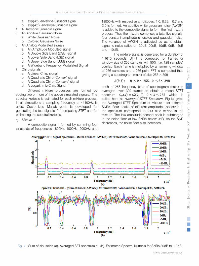
18000Hz with respective amplitudes: 1.0, 0.25, 0.7 and 2.0 is formed. An additive white gaussian noise (AWGN) is added to the composite signal to form the first mixture process. Thus the mixture comprises a total five signals: four constant amplitude sinusoids and gaussian noise. The variance of AWGN is adjusted so as to obtain signal-to-noise ratios of 30dB, 20dB, 10dB, 0dB, -5dB and -10dB.

The mixture signal is generated for a duration of 1.1610 seconds. STFT is computed for frames or window size of 256 samples with 50% (i.e. 128 samples) overlap. Each frame is multiplied by a hamming window of 256 samples and a 256-point FFT is computed thus giving a spectrogram matrix of size 256 × 399

𝑆𝑆(𝑘𝑘, 𝑙𝑙) ; 0 ≤ 𝑘𝑘 ≤ 255, 0 ≤ 𝑙𝑙 ≤ 398

each of 256 frequency bins of spectrogram matrix is averaged over 399 frames to obtain a mean STFT spectrum 𝑆𝑆𝑀𝑀(𝑘𝑘) = ⟨𝑆𝑆(𝑘𝑘, . )⟩; 0 ≤ 𝑘𝑘 ≤ 255 which is called here as Averaged STFT Spectrum. Fig.1a gives the Averaged STFT Spectrum of Mixture-1 for different SNRs. Four peaks of different amplitudes observed in the spectrum correspond to four sine waves in the mixture. The low amplitude second peak is submerged in the noise floor at low SNRs below 0dB. As the SNR decreases, the noise floor also increases.

a. exp(-kt) envelope Sinusoid signalb. exp(-kt2) envelope Sinusoid signal

4. A Harmonic Sinusoid signal5. An Additive Gaussian Noise

a. White Gaussian Noiseb. Colored Gaussian Noise

6. An Analog Modulated signalsa. An Amplitude Modulted signalb. A Double Side Band (DSB) signalc. A Lower Side Band (LSB) signald. A Upper Side Band (USB) signale. A Wideband Frequency Modulated Signal

7. Chirp signalsa. A Linear Chirp signalb. A Quadratic Chirp (Convex) signalc. A Quadratic Chirp (Concave) signald. A Logarithmic Chirp Signal

Fig. 1 : Sum of sinusoids (a). Averaged SFT spectrum of (b). Estimated Spectral Kurtosis for SNRs 30dB to -10dB



Globa

l Jo

urna

l of

Resea

rche

s in E

nginee

ring

()

Volum

Year

2015

54

Fe

XV

Issu

e VI V

ersion

I

The spectral kurtosis К𝑆𝑆(𝑘𝑘); 0 ≤ 𝑘𝑘 ≤ 255 is also computed from the spectrogram matrix using eq.(28) as explained in section IV. It may be noted that К𝑆𝑆(0) is to be ignored, as the kurtosis is not defined at 𝑓𝑓 = 0. The Fig.1b gives the spectral kurtosis (SK) of Mixture-1 for different SNRs.

The spectral kurtosis has four negative peaks corresponding to four sinusoids. For higher SNR (30dB) the peaks have a value of -1 irrespective of the sinusoid amplitudes. As the SNR decreases, the peaks values increase from -1 towards zero. Local SNR computed at peak locations vary depending upon the amplitude of the sinusoid. Here it is maximum at 18000Hz and minimum at 4000Hz. It may be noted down that the SNR referred in the legend of the figures1(a) and (b) is the global SNR, which is computed based on the aggregate of all sinusoids. For global SNRs below 0dB, where the AWGN power dominates the aggregate power of all

sinusoids, the mixture becomes more and more gaussian, the spectral kurtosis tends to zero, relatively faster at 4000Hz where the local SNR is minimum.b) Mixture-2

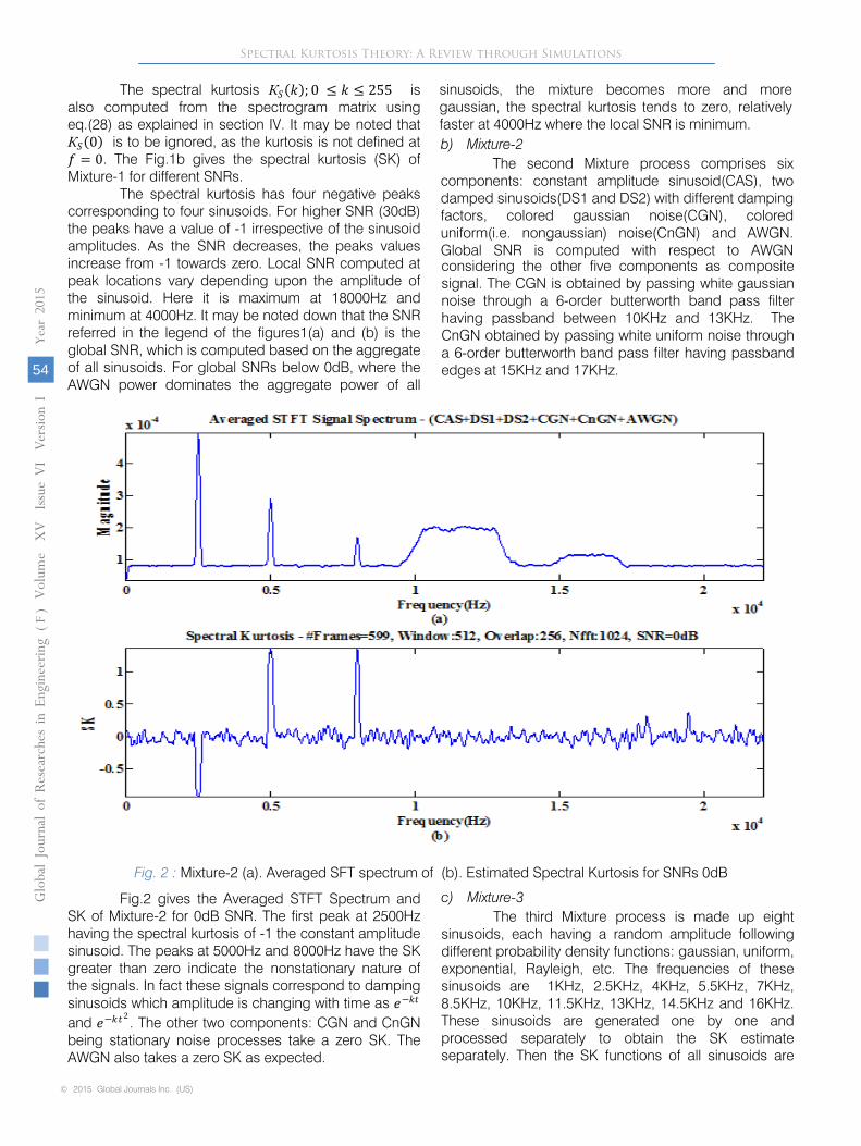
The second Mixture process comprises six components: constant amplitude sinusoid(CAS), two damped sinusoids(DS1 and DS2) with different damping factors, colored gaussian noise(CGN), colored uniform(i.e. nongaussian) noise(CnGN) and AWGN. Global SNR is computed with respect to AWGN considering the other five components as composite signal. The CGN is obtained by passing white gaussian noise through a 6-order butterworth band pass filter having passband between 10KHz and 13KHz. The CnGN obtained by passing white uniform noise through a 6-order butterworth band pass filter having passband edges at 15KHz and 17KHz.

Fig. 2 : Mixture-2 (a). Averaged SFT spectrum of (b). Estimated Spectral Kurtosis for SNRs 0dB

Fig.2 gives the Averaged STFT Spectrum and SK of Mixture-2 for 0dB SNR. The first peak at 2500Hz having the spectral kurtosis of -1 the constant amplitude sinusoid. The peaks at 5000Hz and 8000Hz have the SK greater than zero indicate the nonstationary nature of the signals. In fact these signals correspond to damping sinusoids which amplitude is changing with time as 𝑒𝑒−𝑘𝑘𝑡𝑡

and 𝑒𝑒−𝑘𝑘𝑡𝑡2. The other two components: CGN and CnGN

being stationary noise processes take a zero SK. The AWGN also takes a zero SK as expected.

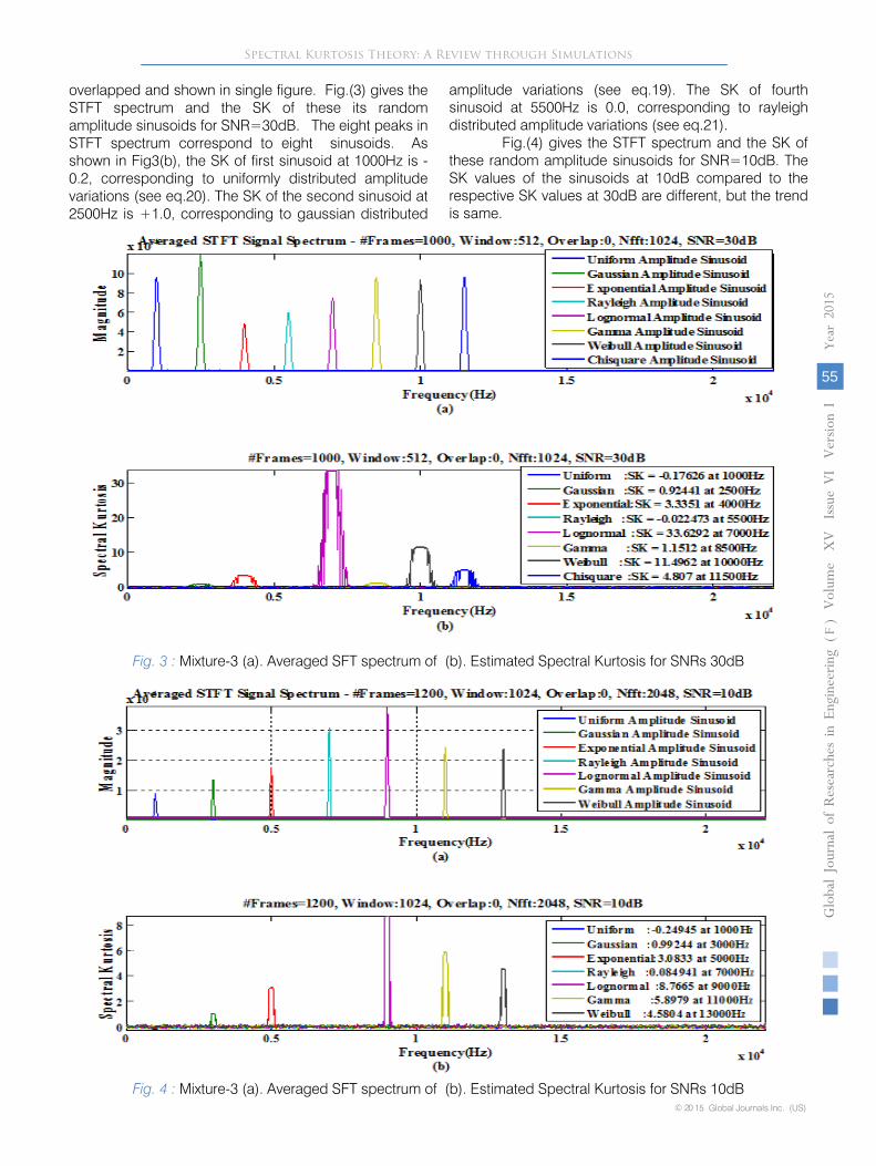
c) Mixture-3The third Mixture process is made up eight

sinusoids, each having a random amplitude following different probability density functions: gaussian, uniform, exponential, Rayleigh, etc. The frequencies of these sinusoids are 1KHz, 2.5KHz, 4KHz, 5.5KHz, 7KHz, 8.5KHz, 10KHz, 11.5KHz, 13KHz, 14.5KHz and 16KHz. These sinusoids are generated one by one and processed separately to obtain the SK estimate separately. Then the SK functions of all sinusoids are



Globa

l Jo

urna

l of

Resea

rche

s in E

nginee

ring

()

Volum

e X

V

Issu

e VI V

ersion

I

55

Year

2015

F

overlapped and shown in single figure. Fig.(3) gives the STFT spectrum and the SK of these its random amplitude sinusoids for SNR=30dB. The eight peaks in STFT spectrum correspond to eight sinusoids. As shown in Fig3(b), the SK of first sinusoid at 1000Hz is -0.2, corresponding to uniformly distributed amplitude variations (see eq.20). The SK of the second sinusoid at 2500Hz is +1.0, corresponding to gaussian distributed

amplitude variations (see eq.19). The SK of fourth sinusoid at 5500Hz is 0.0, corresponding to rayleigh distributed amplitude variations (see eq.21).

Fig.(4) gives the STFT spectrum and the SK of these random amplitude sinusoids for SNR=10dB. The SK values of the sinusoids at 10dB compared to the respective SK values at 30dB are different, but the trend is same.





Globa

l Jo

urna

l of

Resea

rche

s in E

nginee

ring

()

Volum

Year

2015

56

Fe

XV

Issu

e VI V

e rsion

I

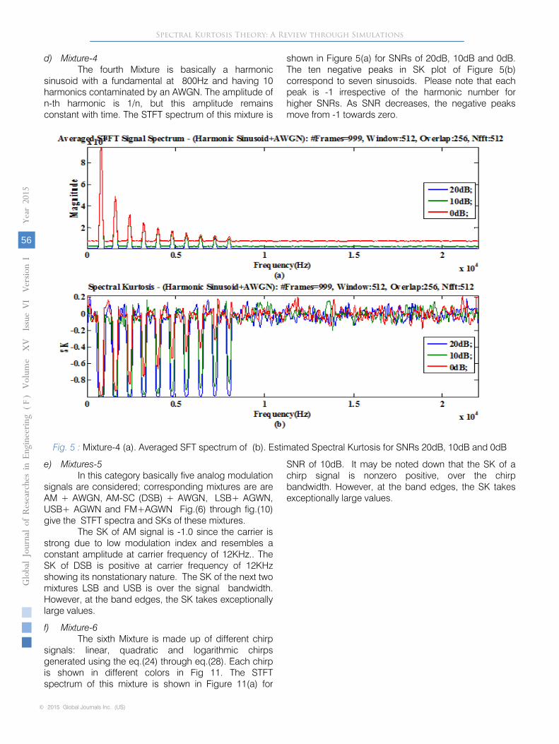
d) Mixture-4The fourth Mixture is basically a harmonic

sinusoid with a fundamental at 800Hz and having 10 harmonics contaminated by an AWGN. The amplitude of n-th harmonic is 1/n, but this amplitude remains constant with time. The STFT spectrum of this mixture is

shown in Figure 5(a) for SNRs of 20dB, 10dB and 0dB. The ten negative peaks in SK plot of Figure 5(b) correspond to seven sinusoids. Please note that each peak is -1 irrespective of the harmonic number for higher SNRs. As SNR decreases, the negative peaks move from -1 towards zero.

Fig. 5 : Mixture-4 (a). Averaged SFT spectrum of (b). Estimated Spectral Kurtosis for SNRs 20dB, 10dB and 0dB

e) Mixtures-5In this category basically five analog modulation

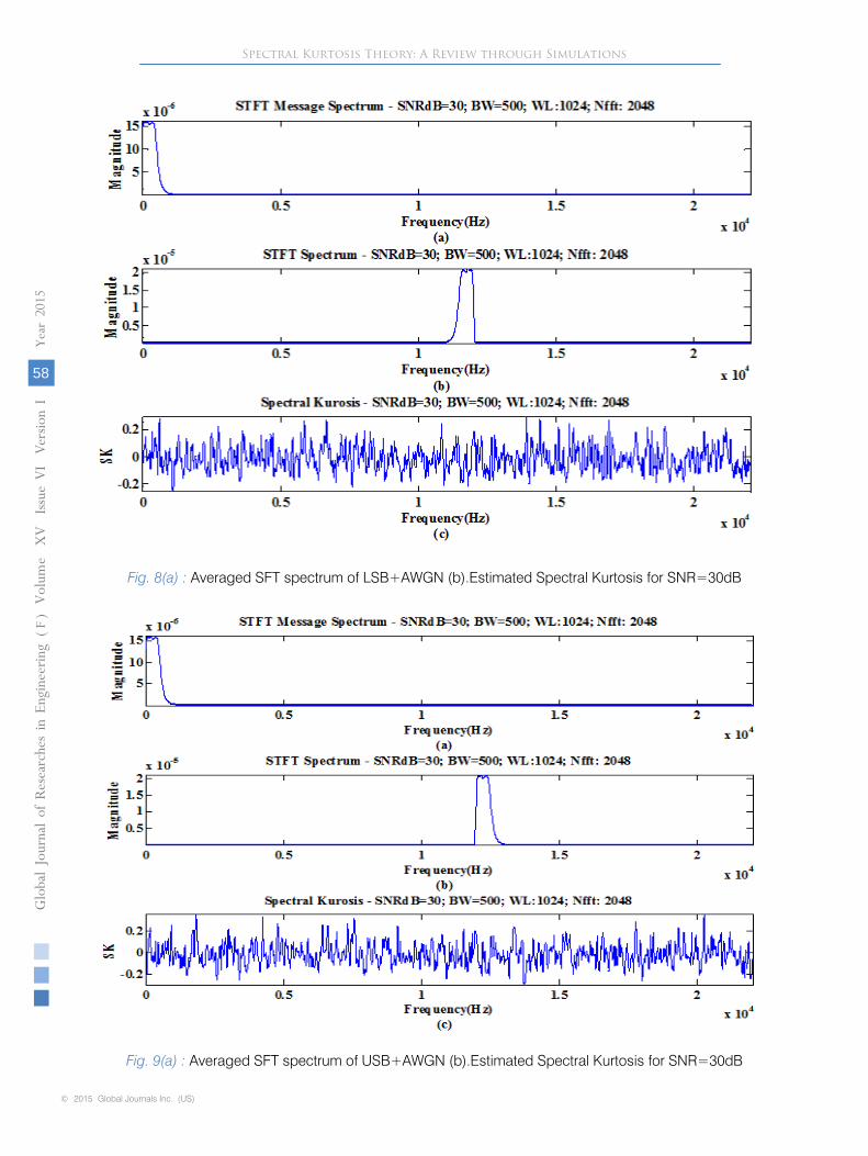
signals are considered; corresponding mixtures are are AM + AWGN, AM-SC (DSB) + AWGN, LSB+ AGWN, USB+ AGWN and FM+AGWN Fig.(6) through fig.(10) give the STFT spectra and SKs of these mixtures.

The SK of AM signal is -1.0 since the carrier is strong due to low modulation index and resembles a constant amplitude at carrier frequency of 12KHz.. The SK of DSB is positive at carrier frequency of 12KHz showing its nonstationary nature. The SK of the next two mixtures LSB and USB is over the signal bandwidth. However, at the band edges, the SK takes exceptionally large values.

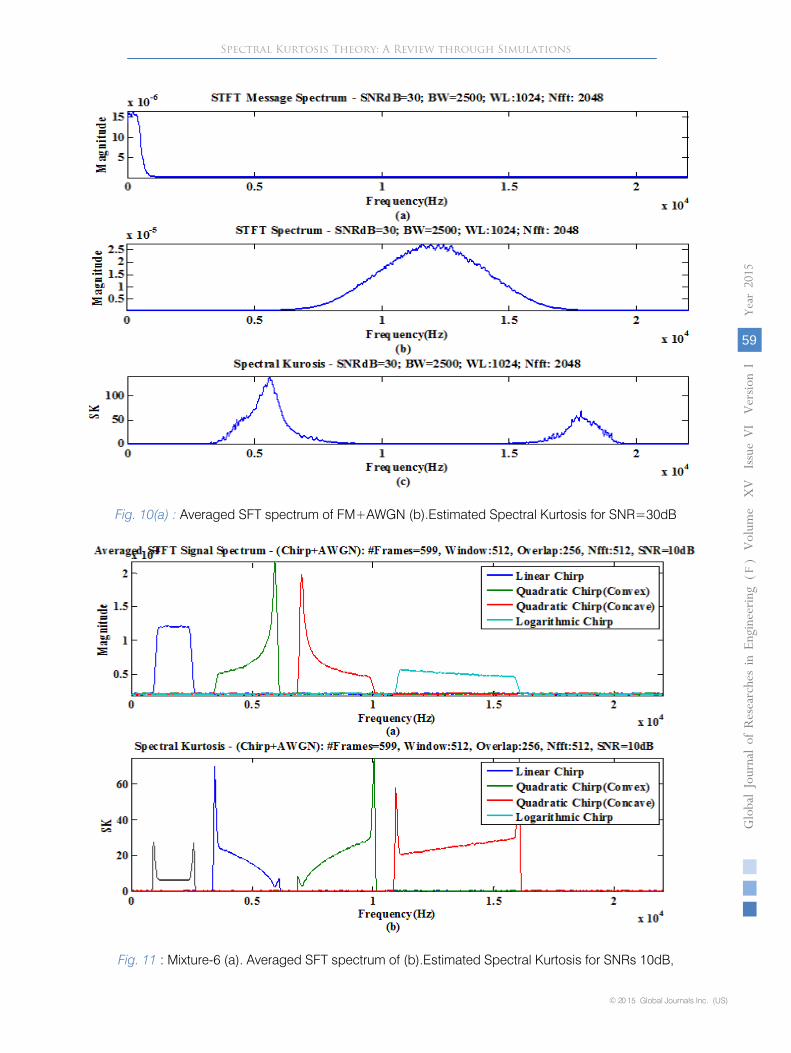
f) Mixture-6The sixth Mixture is made up of different chirp

signals: linear, quadratic and logarithmic chirps generated using the eq.(24) through eq.(28). Each chirp is shown in different colors in Fig 11. The STFT spectrum of this mixture is shown in Figure 11(a) for

SNR of 10dB. It may be noted down that the SK of a chirp signal is nonzero positive, over the chirp bandwidth. However, at the band edges, the SK takes exceptionally large values.

https://www.google.co.in/search?tbo=p&tbm=bks&q=inauthor:%22Randy+Goldberg%22�

https://www.google.co.in/search?tbo=p&tbm=bks&q=inauthor:%22Lance+Riek%22�

http://ieeexplore.ieee.org/search/searchresult.jsp?searchWithin=%22Authors%22:.QT.Makloi%2C%20N..QT.&newsearch=true�

http://ieeexplore.ieee.org/search/searchresult.jsp?searchWithin=%22Authors%22:.QT.Chayawan%2C%20C..QT.&newsearch=true�



Globa

l Jo

urna

l of

Resea

rche

s in E

nginee

ring

()

Volum

e X

V

Issu

e VI V

ersion

I

57

Year

2015

F

Fig. 6 (a) : Averaged SFT spectrum of AM+AWGN (b).Estimated Spectral Kurtosis for SNR=30dB

Fig. 7(a) : Averaged SFT spectrum of DSB+AWGN (b).Estimated Spectral Kurtosis for SNR=30dB


Globa

l Jo

urna

l of

Resea

rche

s in E

nginee

ring

()

Volum

Year

2015

58

Fe

XV

Issu

e VI V

e rsion

I


Fig. 8(a) : Averaged SFT spectrum of LSB+AWGN (b).Estimated Spectral Kurtosis for SNR=30dB

Fig. 9(a) : Averaged SFT spectrum of USB+AWGN (b).Estimated Spectral Kurtosis for SNR=30dB


Globa

l Jo

urna

l of

Resea

rche

s in E

nginee

ring

()

Volum

e X

V

Issu

e VI V

ersion

I

59

Year

2015

F


Fig. 10(a) : Averaged SFT spectrum of FM+AWGN (b).Estimated Spectral Kurtosis for SNR=30dB

Fig. 11 : Mixture-6 (a). Averaged SFT spectrum of (b).Estimated Spectral Kurtosis for SNRs 10dB,


Globa

l Jo

urna

l of

Resea

rche

s in E

nginee

ring

()

Volum

Year

2015

60

Fe

XV

Issu

e VI V

e rsion

I


VI. Conclusions and Future Work

The cumulant based spectral kurtosis defined in frequency domain originally proposed for bearing fault detection and monitoring of electrical machines, is a promising tool for analyzing nonstationary signals. It complements the traditional power spectrum based on second order statistics. In this paper, the theory of spectral kurtosis is briefly reviewed from the fundamentals. The properties of spectral kurtosis of popular stationary signals, nonstationary signals and mixed processes are analytically given. Extensive Monte Carlo simulations were carried out to support the theory. The spectral kurtosis of the simulated stationary, nonstationay and mixed processes at different signal-to-noise ratios (SNRs) is estimated and the results are in good match with the previous analytical findings. The review highlights the usage of spectral kurtosis for other areas of signal processing like communications and radar signal processing. Future work could be (i). Obtaining closed-form expressions for spectral kurtosis of communication and radar signals (analog or digital modulated) (ii). classification of communication signals using spectral kurtosis at different SNRs.(iii). radar signal classification using spectral kurtosis.

References Références Referencias

1. E. Scheier and M. Slaney, “Construction and evaluation of a robust multifeature speech/ music discriminator,” Proc. IEEE,ICASSP-97, 1997.

2. E. Wold, T. Blum, D. Keislar, and J. Wheaton, “Content-based classification, search, and retrieval of audio,” IEEE Multimedia Mag., vol. 3, pp. 27–36, Fall 1996.

3. Peeters, G., Burthe, A. L. and Rodet, X., ”Toward automatic music audio summary generation from signal analysis”, Proceedings of the Third International Conference on Music Information Retrieval, pp. 94-100, 2002, Paris, France.

4. Eberhard Hänsler and Gerhard Schmidt (editors), “Speech and Audio Processing in Adverse Environments”, Springer, 2008.

5. Randy Goldberg, and Lance Riek, “A Practical Handbook of Speech Coders”, CRC Press, 2000, pp.200-203.

6. Pham Chau Khoa and Chng Eng Siong, “Spectral local harmonicity feature for voice activity detection”, International Conference on Audio, Language and Image Processing (ICALIP), Shanghai , 2012, pp.407 – 413

7. Merrill I. Skolnik, ”Introduction to Radar Systems”, Second edition, McGraw-Hill, 1980, pp.46-50.

8. Makloi, N. and Chayawan, C., ”Performance evaluation of wireless communications using equal gain diversity combining in a nongaussian multipath fading environment”, TENCON 2004. IEEE Region 10 Conference, 2004, Vol. 2, pp.613 – 616.

9. Yi Chen et. al., ”Exact Non-Gaussian Interference Model for Fading Channels”, IEEE Transactions on Wireless Communications”, Volume: 12, 2013, Issue: 1, pp.168 - 179,

10. Keh-Shin Lii, ”Identification and Estimation of Non-Gaussian ARMA Processes”, IEEE Trans on Acoustics, Speech and Signal Processing, Vol.38, No.7, July 1990, pp.1266-1276.

11. Ananthram Swami and Jerry M. Mendel, ” Cumulant-Based Approach to the Harmonic Retrieval and related Problems”, IEEE Trans on Signal Processing, Vol.39, No.5, March 1991, pp.1099-1108.

12. Georgios B. Giannakis and Jerry M. Mendel,”Identification of Non-minimum phase systems using Higher Order Statistics”, IEEE Trans on Acoustics, Speech and Signal Processing, Vol.37, No.3, March 1989, pp.360-377.

13. Sawalhi, N. and Randall, R, “The application of spectral kurtosis to bearing diagnostics”, Proceedings of Acoustics-2004, 3-5 November 2004, Gold Coast, Australia, pp. 393-398.

14. Wang, Y. and Liang, M.. “An adaptive SK technique and its application for fault detection of rolling element bearings”, Mechanical Systems and Signal Processing, Vol. 25, pp. 1750–1764.

15. Chun Li et. al., ”Bearing Fault Detection by resonant frequency band persuit using a synthesized criterion,”proc 3rd Int. conf. on Mechnanical engineering and Mechatronics, Prague, 14-15 August 2014, pp.37.1 -37.8.

16. J. Antoni and R. Randall, “The spectral kurtosis: application to the vibratory surveillance and diagnostics of rotating machines”, Mechanical Systems and Signal Processing, vol. 20, no. 2, pp. 308 -331, 2006.

17. R. Dwyer, ”Detection of non-gaussian signals by frequency domain kurtosis estimation”, Proc. Int. Conf. on Acoustics, Speech and Signal Processing, ICASSP-83, vol. 8, 1983, pp. 607-610.

18. Valeriu Vrabie et. al., "Spectral Kurtosis: From Definition To Application", 6th IEEE International Workshop on Nonlinear Signal and Image Processing, NSIP-2003, Grado-Trieste, Italy, pp.1-5.

19. J. Antoni, “The Spectral Kurtosis of Nonstationary Signals: Formalisation, Some Properties, And Application”, 12th European Signal Processing Conference, Vienna, Austria, 2004.

20. J. Antoni, “The spectral kurtosis: a useful tool for characterizing nonstationary signals”, Mechanical Systems and Signal Processing, vol. 20, no. 2, pp. 282 - 307, 2006.

21. J. Antoni, “Fast computation of the kurtogram for the detection of transient faults”, Mechanical Systems and Signal Processing, vol. 21, pp. 108-124, Jan. 2007.


Globa

l Jo

urna

l of

Resea

rche

s in E

nginee

ring

()

Volum

e X

V

Issu

e VI V

ersion

I

61

Year

2015

F


22. E. Nemer, R. Goubran, and S. Mahmoud, “SNR estimation of speech signals using subbands and fourth-order statistics”, IEEE Signal Process. Lett., vol. 6, no. 7, pp. 171-174, Jul. 1999.

23. P. Ravier and P. O. Amblard, “Denoising using wavelet packets and the kurtosis: application to transient detection”, Proc. IEEE-SP International Symposium on Time-Frequency and Time-Scale Analysis, 6_9 Oct.1998, pp. 625-628.

24. J. J. G. de la Rosa, C. G. Puntonet, and A. Moreno, “Subterranean termite detection using the spectral kurtosis”, Proc. 4th IEEE Workshop on Intelligent Data Acquisition and Advanced Computing Systems: Technology and Applications IDAACS 2007, 2007, pp. 351-354.

25. Valeriu Vrabie et. al., " Application of Spectral Kurtosis To Bearing Fault Detection in Induction Motors", Surveilance 5 CETIM Senlis 11-13 October 2004.

26. Athanasios Papoulis and S.Unnikrishna Pillai, ”Probability, Random Variables and Stochastic Processes”, Fourth edition, Tata McGraw-Hill, 2002, pp.146-148.

27. Jerry M. Mendel, ”Tutorial on Higher Order Statistics(Spectra) in Signal Processing and System Theory: Theoretical Results and Some Applications”, IEEE Trans on Acoustics, Speech and Signal Processing, Vol.37, No.3, March 1989, pp.278-305, proc IEEE, Vol.79, No.3, March 1991.

by venkata krishna rao m - globaljournals.org filespectral kurtosis theory: a review through...

Documents