by suched likitlersuang balliol college michaelmas term … · 2013-07-26 · suched likitlersuang...
TRANSCRIPT

A HYPERPLASTICITY MODEL FOR CLAY BEHAVIOUR: AN APPLICATION TO BANGKOK CLAY
by
Suched Likitlersuang
Balliol College
Michaelmas Term 2003
A thesis submitted for the degree of Doctor of Philosophy at the
University of Oxford

i
A HYPERPLASTICITY MODEL FOR CLAY BEHAVIOUR: AN APPLICATION TO BANGKOK CLAY
by
Suched Likitlersuang
Balliol College
Michaelmas Term 2003
A thesis submitted for the degree of Doctor of Philosophy at the
University of Oxford
ABSTRACT The main purpose of this thesis is the development of a new constitutive soil
model emphasising the use of thermodynamic principles. This new approach to
plasticity modelling, termed ‘hyperplasticity’, was first developed by Collins and
Houlsby (1997) and Houlsby and Puzrin (2000). This idea has been further extended
to continuous hyperplasticity in which smooth transitions between elastic and plastic
behaviour can be modelled (Puzrin and Houlsby, 2001b). Applying hyperplasticity to
this researh, a kinematic hardening model specified by means of two scalar
functionals is used to accommodate the effect of stress history on stiffness. A rate-
dependent calculation for an approximation of the incremental stress-strain response
is introduced. The model developed in the research is named ‘kinematic hardening
modified Cam-clay (KHMCC) model’ and requires eight parameters (plus an extra
parameter for rate-dependent analysis). Triaxial test results from the Asian Institute
of Technology (AIT) and cyclic undrained triaxial data from Chulalongkorn
University are employed to establish the soil parameters for the new model. The
model is initially developed in terms of triaxial stress-strain parameters for the
purpose of comparison with the experimental data on Bangkok clay. The model is
expressed in FORTRAN code for implementation into the OXFEM finite element
program. Two examples of real geotechnical projects in Bangkok (a road
embankment and tunnelling in soft ground) are analysed under plane strain
conditions. Comparisons of the numerical analysis results with field data are made.
In addition, factors affecting the results of the analysis such as stress history and K0,
are investigated.

ii
ACKNOWLEDGEMENT
The research would not have been possible without the support of many people
whom it is appropriate to acknowledge and thank.
Firstly, I would like to express my profound gratitude and sincere appreciation
to Professor Guy T. Houlsby for giving valuable suggestions and guidance throughout
my research. I would like to extend my gratitude to Chair Professor A.S.
Balasubramaniam for providing triaxial experimental data from AIT. I am also
thankful to Assistant Professor Supot Teachavorasinskun for offering a set of cyclic
undrained triaxial data from Chulalongkorn University.
Most importantly the support staff and friends in the Civil Engineering research
group, I specially thank Dr. Harvey J. Burd for his recommendation on the OXFEM
finite element program as well as its numerical implementation. I owe a debt of
gratitude to many of my colleagues, in particular to Nguyen Dinh Giang and John
Pickhaver and the support staffs, Alison, Karen, Bob as well as the old secretary,
Nicola.
I am very grateful to all of my lecturers at Chulalongkorn University for
providing general civil engineering background during my study in undergraduate
level. The knowledge imparted to me by all the lecturers at AIT during the masters
course of my study helped strengthen my knowledge in geotechnical engineering.
I appreciate many helpful discussions with Jarungwit Wongsaroj, who is
undergoing a numerical research on tunnelling at Cambridge University. I would also
like to thank, Nopphol Witvorapong (B.A., PPE, St. Hugh’s college) and Paradorn
Rangsimaporn (D.Phil student, Department of Politics and IR, St. Antony’s college)
for their generous proof and corrections of my thesis draft.
I owe greatest debt of gratitude to my family for their continuous inspiration and
moralistic as well as financial support for the first two years of my course. I also
acknowledge with gratitude my sponsorship, the Thai Royal Government, for the last
year of my course.
Over the course of my doctorate I have many friends throughout the Oxford
University in particular in Balliol College, Holywell Manor, 49 Banbury Road and
Thai Society. Many thanks are due to all my friends at Oxford University.
TABLE OF CONTENTS
iii
TABLE OF CONTENTS No. Content Page
ABSTRACT……………………………………………………………. i
ACKNOWLEDGEMENT……………………………………………. ii
TABLE OF CONTENTS……………………………………………... iii
LIST OF SYMBOLS………………………………………………….. vii
Chapter 1 Introduction
1.1 Real soil behaviour……………………………………………………. 1-1
1.2 Problems associated with soil models…………………………………. 1-3
1.3 Research objectives and structure of the thesis………………………... 1-7
Chapter 2 Constitutive model for soil
2.1 Constitutive models for soil…………………………………………...... 2-1
2.2 Classical soil models…………………………………………………..... 2-2
2.3 Development in soil models……………………………………………. 2-4
2.3.1 The bounding surface concept……………………………………. 2-4
2.3.2 Kinematic yield surface concept…………………………………. 2-6
2.4 Some recently developed soil models………………………………….. 2-7
2.4.1 A kinematic hardening model (KH)……………………………… 2-8
2.4.2 Three-surface kinematic hardening model (3-SKH)……………... 2-11
2.4.3 The MIT soil model…………………………………………….… 2-14
2.5 Evaluation and prediction of models…………………………………… 2-20
2.5.1 A kinematic hardening model (KH)……………………………… 2-21
2.5.2 Three-surface kinematic hardening model (3-SKH)……………... 2-25
2.5.3 The MIT-E3 model (MIT-E3)…………………………………… 2-28
2.6 Comparison of models…………………………………………………. 2-32
Chapter 3 Hyperplasticity Theory
3.1 Hyperplasticity theory…………………………………………………. 3-1
3.2 Hyperplasticity model for rate-dependent material……………………. 3-2
3.3 Multiple internal variables and continuous internal function………….. 3-5
3.4 Strain hardening model………………………………………………… 3-7
TABLE OF CONTENTS
iv
3.3.1 Isotropic hardening model……………………………………….. 3-8
3.3.2 Kinematic hardening model……………………………………… 3-9
3.5 Kinematic hardening function for a continuous hyperplasticity model.. 3-10
3.6 Hyperplasticity models for soil mechanics…………………………….. 3-12
3.6.1 Elastic model…………………………………………………….. 3-13
3.6.2 Elasto-platic model with single internal variable……………….. 3-17
3.6.3 Elasto-plastic model with single kinematic internal variable…… 3-21
3.6.4 Elasto-plastic model with multiple kinematic internal variables.. 3-24
3.6.5 Elasto-plastic model with continuous kinematic internal function 3-27
3.7 Continuous hardening function………………………………………..... 3-30
3.7.1 Linear volumetric stress-strain relation.………………………….. 3-30
3.7.2 Logarithmic volumetric stress-strain relation…………………….. 3-34
3.8 Summarised tables of the hyperplasticity soil model…………………... 3-36
3.9 Calculation algorithms…………………………………………………. 3-40
3.9.1 Rate independent formulation……………………………………. 3-40
3.9.2 Example of rate-independent triaxial test…………..…………….. 3-42
3.9.3 Rate dependent formulation……………………………………..... 3-43
3.9.4 Example of rate-dependent triaxial test…………..………………. 3-45
3.9.5 Comparison between two approaches……………………………. 3-45
Chapter 4 Review of experimental work
4.1 Geology condition…………………………………………………….... 4-1
4.2 Experimental program…………………………………………………. 4-3
4.2.1 Sample preparation………………………………………………. 4-3
4.2.2 Equipment accuracy…………………………………………….... 4-4
4.2.3 Testing program………………………………………………….. 4-5
4.3 AIT experimental data………………………………………………….. 4-6
4.4 Consolidation data……………………………………………………… 4-7
4.4.1 Isotropic consolidation data from triaxial test………………….… 4-8
4.4.2 Anisotropic consolidation data from triaxial test……………….... 4-8
4.4.3 Consolidation data from Oedometer……………………………... 4-11
4.4.4 Consolidation data from CRS test………………………………... 4-12
4.5 Undrained shear data………………………………………………….... 4-13

TABLE OF CONTENTS
v
4.6 Drained shear data……………………………………………………... 4-15
4.7 Cyclic undrained data………………………………………………….. 4-17
4.8 Conclusion……………………………………………………………… 4-19
Chapter 5 Comparison, Results and Discussion
5.1 Implementation in FORTRAN code………………………………….... 5-2
5.2 Consolidation behaviour prediction……………………………………. 5-3
5.3 Isotropic behaviour prediction…………………………………………. 5-6
5.3.1 Isotropic undrained behaviour………………………………….… 5-6
5.3.2 Isotropic drained behaviour…………………………………….… 5-9
5.4 Anisotropic behaviour prediction…………………………………….… 5-11
5.4.1 Anisotropic undrained behaviour………………………………… 5-12
5.4.2 Anisotropic drained behaviour…………………………………… 5-17
5.5 Cyclic behaviour prediction……………………………………………. 5-19
5.6 Conclusion and Future work………………………………………….... 5-24
Chapter 6 Implementation into Finite Element Code
6.1 Stress-strain definition…………………………………………………. 6-1
6.2 Generalised soil models………………………………………………... 6-2
6.3 Two-dimensional soil models for OXFEM…………………………..… 6-4
6.4 Solution scheme………………………………………………………... 6-5
6.4.1 Incremental stress-strain solution at element level………………. 6-5
6.4.2 Modified Newton-Raphson (MNR) method……………………... 6-5
6.5 Choice of element type……………………………………………….… 6-8
6.6 Analysis type…………………………………………………………… 6-8
6.7 Test problems……………………………………………………….….. 6-9
6.8 Comparison of results………………………………………………….. 6-10
6.9 Conclusion……………………………………………………………… 6-14
Chapter 7 Application to Geotechnical problems
7.1 Road embankment……………………………….…………………….. 7-1
7.1.1 Embankment geometry and soil conditions……………………… 7-2
7.1.2 Data collection………………………………………………….... 7-3
TABLE OF CONTENTS
vi
7.1.3 Finite element mesh…………………………………………….... 7-4
7.1.4 Constitutive models…………………………………………….… 7-5
7.1.5 Analysis results…………………………………………………... 7-6
7.2 Tunnelling………………………………………………………………. 7-18
7.2.1 Empirical prediction of tunnelling-induced settlement…………... 7-18
7.2.2 Model ground condition and input soil properties……………….. 7-19
7.2.3 Model of lining………………………………………………….... 7-20
7.2.4 Finite element mesh……………………………………………..... 7-21
7.2.5 Choice of constitutive model……………………………………... 7-22
7.2.6 Analysis result……………………………………………………. 7-23
7.3 Conclusion……………………………………………………………… 7-33
Chapter 8 Concluding remarks
8.1 Summary of research…………………………………………………… 8-1
8.1.1 Theoretical soil models………………………………………….... 8-1
8.1.2 Evaluation of model parameters………………………………….. 8-2
8.1.3 Implementations to software……………………………………... 8-2
8.1.4 Applications……………………………………………………… 8-3
8.2 Conclusions…………………………………………………………….. 8-3
8.3 Recommendations……………………………………………………… 8-7
REFERENCES……………………………………………………….. 9-1
APPENDIX A: New OXFEM input………………………………….. A-1
APPENDIX B: FORTRAN code for MCC and KHMCC model…... A-3
LIST OF SYMBOLS
vii
LIST OF SYMBOLS
Symbol Meaning a KHMCC model parameter controlling rate of change of stiffness ap KHMCC model parameter a for p term in triaxial model aq KHMCC model parameter a for q term in triaxial model b KHMCC model parameter controlling rate of change of stiffness b parameter related to effect of immediate principal stress bp KHMCC model parameter b for p term in triaxial model bq KHMCC model parameter b for q term in triaxial model c friction stress in slip component ci friction stress in each slip component of multiple yield surface model c friction function in slip component of infinite yield surface model c′ cohesion parameter (Mohr-Coulomb failure criteria)
*c mathematical constraint d dissipation function
inG∆d vector of incremental nodal displacements
e void ratio e choice of four energy potentials (u, f, h, g) f specific Helmholtz free energy cf ′ compressive strength of concrete
iG∆f vector of incremental nodal forces
g specific Gibbs free energy gx shear modulus gradient g shear modulus function h specific enthalpy hc damping ratio i trough width parameter p mean effective stress (triaxial stress parameter) p0 reference pressure (KHMCC model) pa reference pressure (power function of modulus) pc reference pressure (MCC model) pini initial pressure (after consolidation) pm maximum past pressure px reference of yield surface q deviatoric stress (triaxial stress parameter) qu unconsolidated undrained shear strength r KHMCC model parameter controlling plastic stiffness n number of yield surface n degree of power function s specific entropy su undrained shear strength t time u specific internal energy u∆ excess pore pressure
u, v, w displacement components in Cartesian coordinates v specific volume w flow potential (rate-independent material)
LIST OF SYMBOLS
viii
y yield function iy each yield function of multiple yield surface model
y yield functional of infinite yield surface model z force potential (rate-dependent material) z depth
AS axi-symmetry condition CID isotropic consolidated drained triaxial compression test CIU isotropic consolidated undrained triaxial compression test
CK0DC K0 consolidated drained triaxial compression test CK0DE K0 consolidated drained triaxial extension test CK0UC K0 consolidated undrained triaxial compression test CK0UE K0 consolidated undrained triaxial extension test
CR compression ratio CRS constant rate of strain consolidometer test CSL critical state line
CSSM critical state soil mechanics E elastic Young’s modulus E ′ drained Young’s modulus E50 secant Young’s modulus at 50% of strength Ep plastic Young’s modulus
Esec secant Young’s modulus at particular stress ET tangential Young’s modulus Eu undrained Young’s modulus
EVM elastic Von Mises model FEM finite element method
G elastic shear modulus Gini initial shear modulus Gsec secant shear modulus at particular stress H hardening parameter Hp hardening parameter for p term Hq hardening parameter for q term
iH each of hardening parameters of multiple yield surface model
piH each of p-hardening parameters of multiple yield surface model
qiH each of q-hardening parameters of multiple yield surface model H hardening function of infinite yield surface model
pH p-hardening function of infinite yield surface model
qH q-hardening function of infinite yield surface model I1 first stress invariant J cross-coupling between shear and volumetric stress-strain J2 second stress invariant J3 third stress invariant K elastic bulk modulus K in-situ stress ratio ( vhK σσ= ) K0 coefficient of earth pressure at rest Ka coefficient of active pressure Ke elastic stiffness matrix
iGK incremental global stiffness matrix

LIST OF SYMBOLS
ix
Kp plastic bulk modulus Ksec secant bulk modulus at particular stress KT tangential Young’s modulus
KHMCC kinematic hardening modified Cam-clay model M slope of critical state line MC magnitude of critical state cone in compression side ME magnitude of critical state cone in extension side
MCC modified Cam-clay model N number of testing cycles
NCL normal consolidated line OCR overconsolidated ratio
OXFEM Oxford finite element program Pa active force PS plane strain condition RR recompression ratio S transverse settlement trough due to tunnel excavation maxS maximum settlement above tunnel axis
SBS state boundary surface UU unconsolidated undrained shear test VL volume loss α internal variable α& rate of change of internal variable
iα each of internal variables
iα each of internal variable functions
ijα internal variable tensor
ijα& rate of change of internal variable tensor
ijα internal variable tensor function
pα internal variable for p term in triaxial model
piα each of internal variables for p term in triaxial model
pα internal variable function for p term in triaxial model
qα internal variable for q term in triaxial model
qiα each of internal variables for q term in triaxial model
qα internal variable function for q term in triaxial model β modified isotropic hardening variable γ engineering shear strain
yzxzxy γγγ ,, direction shear components in Cartesian coordinates
zrrz θθ γγγ ,, direction shear components in cylindrical coordinates
SAγ single amplitude shear strain ε one-dimensional strain ε& rate of change of strain
321 ,, εεε major, intermediate, minor principal strain
vh εε , horizontal and vertical strain
zyx εεε ,, direction strain components in Cartesian coordinates
LIST OF SYMBOLS
x
θεεε ,, rz direction strain components in cylindrical coordinates
vε volumetric strain
ijε strain tensor evε elastic volumetric strain p
vε plastic volumetric strain
sε shear strain esε elastic shear strain psε plastic shear strain η internal coordinate η stress ratio (q/p)
*η active internal coordinate θ temperature θ Lode’s angle κ slope of swelling line (e – ln p plot)
*κ slope of swelling line (ln v – ln p plot) κ ′ slope of swelling line at half of maximum past stress λ slope of NCL (e – ln p plot) λ arbitrary non-negative multiplier for Legendre-Fenchel transformation
*λ slope of NCL (ln v – ln p plot) λ λ function µ viscosity coefficient υ Poisson’s ratio υ′ angle of dilation υ′ drained Poisson’s ratio
uυ undrained Poisson’s ratio σ total stress σ& rate of change of stress σ ′ effective stress
0σ reference stress
321 ,, σσσ major, intermediate, minor principal stress
vh σσ ′′ , horizontal and vertical effective stress
00 , vh σσ ′′ horizontal and vertical in-situ effective stress
zyx σσσ ,, direction stress components in Cartesian coordinates
θσσσ ,, rz direction stress components in cylindrical coordinates
mσ maximum past stress
ijσ total stress tensor
ijσ ′ effective stress tensor φ′ friction angle parameter (Mohr-Coulomb failure criteria)
TCφ′ critical state angle of shearing resistance in triaxial compression
TEφ′ critical state angle of shearing resistance in triaxial extension χ dissipative generalised stress χ generalised stress

LIST OF SYMBOLS
xi
ijχ dissipative generalised stress tensor
ijχ generalised stress tensor
pχ dissipative generalised stress for p term in triaxial model
qχ dissipative generalised stress for q term in triaxial model
pχ generalised stress for p term in triaxial model
qχ generalised stress for q term in triaxial model plane−π deviatoric plane Λ arbitrary non-negative multiplier for constraint
Macaulay bracket Bounding surface model parameters, Dafalias and Herrmann (1982) n parameters for non-linear hardening H total stiffness H0 stiffness parameter Hp plastic stiffness at image point δ mapping distance
*σ image stress Kinematic hardening model parameters, Wood (1995) b distance from current stress to conjugate stress k parameter controlling rate of destructuration strain
(p0,0) centre of reference surface (pα,qα) centre of bubble
r size of structure surface r0 initial degree of structure rs reference surface ss structure surface
A destructuration parameter controlling influence of volumetric and distortion strain
B, ψ soil constants controlling contribution and rate of change of hardening θM ratio of semi-axes of yield surface
R size of bubble dε destructuration strain
0η dimensionless shear stress
cσ conjugate stress
Three-surface kinematic hardening model, Atkinson and Stallebrass (1991)
b1 dot product between movement vector from history surface to bounding surface and normal vector at bounding surface
b2 dot product between movement vector from yield surface to history surface and normal vector at history surface
h plastic stiffness h0 elastic stiffness
(p0,0) centre of bounding surface (pa,qa) centre of history surface (pb,qb) centre of yield surface
H1 plastic stiffness parameter 1 H2 plastic stiffness parameter 2
LIST OF SYMBOLS
xii
S size of yield surface T size of history surface β movement vector from history surface to bounding surface γ movement vector from yield surface to history surface ψ hardening modulus parameter MIT-E3 model, Whittle (1993) b direction of yield surface axis h function of critical state cone k half range of critical state cone
( )revrev qp , stress reversal point
cr parameter describing location of current stress state relative to failure surface
xr relative ratio between orientation of yield surface and critical state cone
Cc friction angles parameter measured from triaxial compression tests Ce friction angles parameter measured from triaxial extension tests
C, n material constant characterising non-linear behaviour in unloading H elasto-plastic modulus
( )qp PP , plasticity flow direction ( )qp QQ , yield surface gradient
tS material parameter influencing strain softening behaviour ξ critical state cone axis
pξ , sξ dimensionless parameters relating current stress state to stress reversal state
ζ scalar obtained from the consistency requirement 0κ initial slope of swelling line in v-ln p plot
γ , h dimensionless input parameter for non-linear hardening rule λd plastic scalar multiplier
NCK 0η stress ratio at K0 normally consolidated condition 0Ψ material constant controlling rate yield surface’s rotation
ω parameter describing non-linearity at small strain due to undrained shearing
χ magnitude of reversal strain
Introduction
1-1
Chapter 1 Introduction
In soil mechanics research many constitutive models are currently built in
terms of sophisticated mathematics which can be difficult to employ in geotechnical
engineering practice. This research therefore aims to develop a new constitutive soil
model for application in engineering practice and also to capture the main
characteristics of soil behaviour.
There are many different groups of constitutive equations used to characterise
the stress-strain-strength behaviour of materials. These constitutive models should be
contrasted with the majority of conventional design methods, where much simpler
representations of material behaviour are used. Examples of conventional design
methods are stability analyses, typically assuming rigid perfectly plastic behaviour;
while separate deformation calculations often assume linear elastic behaviour.
1.1 Real soil behaviour Practical analyses of geotechnical problems at this time still often assume
material behaviour to be linear elastic. However, real soils do not simply behave
linear elastically. Real soil behaviour is highly nonlinear, with both strength and
stiffness depending on stress and strain level. For realistic predictions, a more
complex constitutive model is therefore required. Before delving into the constitutive
theory, it is useful to consider real soils and identify some important aspects of their
behaviour. Thus, the following section will begin by considering the behaviour of
soils.
The stress-strain behaviour of soils can be divided into two categories: elastic
and elasto-plastic behaviour. However, it is well established that this behaviour is
controlled by strain amplitude. For instance, soils can be regarded as perfectly elastic
(fully recoverable) only under extremely small strain levels, and as the strain
amplitude increases the apparent stiffness decreases. The most challenging problem
is how to describe, accurately, the smooth transition zone varying from the small
strain level (elastic) to the large strain level (elasto-plastic). Several experimental
researches show that the transition of the stiffness with strain level depends on the
overconsolidation ratio (OCR) and the magnitude of the mean effective stress (p). An
Introduction
1-2
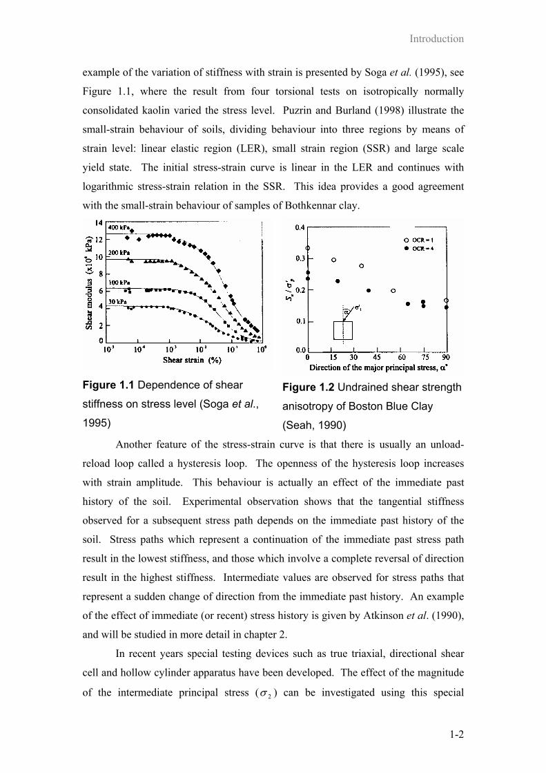
example of the variation of stiffness with strain is presented by Soga et al. (1995), see
Figure 1.1, where the result from four torsional tests on isotropically normally
consolidated kaolin varied the stress level. Puzrin and Burland (1998) illustrate the
small-strain behaviour of soils, dividing behaviour into three regions by means of
strain level: linear elastic region (LER), small strain region (SSR) and large scale
yield state. The initial stress-strain curve is linear in the LER and continues with
logarithmic stress-strain relation in the SSR. This idea provides a good agreement
with the small-strain behaviour of samples of Bothkennar clay.
Figure 1.1 Dependence of shear
stiffness on stress level (Soga et al.,
1995)
Figure 1.2 Undrained shear strength
anisotropy of Boston Blue Clay
(Seah, 1990)
Another feature of the stress-strain curve is that there is usually an unload-
reload loop called a hysteresis loop. The openness of the hysteresis loop increases
with strain amplitude. This behaviour is actually an effect of the immediate past
history of the soil. Experimental observation shows that the tangential stiffness
observed for a subsequent stress path depends on the immediate past history of the
soil. Stress paths which represent a continuation of the immediate past stress path
result in the lowest stiffness, and those which involve a complete reversal of direction
result in the highest stiffness. Intermediate values are observed for stress paths that
represent a sudden change of direction from the immediate past history. An example
of the effect of immediate (or recent) stress history is given by Atkinson et al. (1990),
and will be studied in more detail in chapter 2.
In recent years special testing devices such as true triaxial, directional shear
cell and hollow cylinder apparatus have been developed. The effect of the magnitude
of the intermediate principal stress ( 2σ ) can be investigated using this special

Introduction
1-3
equipment. The relative magnitude of the intermediate principal stress ( 2σ ) is
expressed by the value of 31
32
σσσσ
−−
=b . For example, the undrained shear strength of
undisturbed Haney clay in plane strain condition is some 10% higher than in triaxial
compression, according to Vaid and Campanella (1974).
An anisotropic behaviour of soils is also observed by directional shear testing.
In fact, soils are likely to be isotropic in the plane normal to its deposited direction,
and are therefore called cross anisotropic or transversely isotropic. For instance, the
data on the undrained shear strength of reconsolidated Boston Blue Clay varied the
orientation of the major principal stress ( 1σ ) to the direction of deposition (Seah,
1990). It shows that the undrained shear strength drops by 50% as the angle of 1σ to
the deposited direction increases from 0o-90o as shown in Figure 1.2.
1.2 Problems associated with soil models Due to the complexity of real soil behaviour, a single constitutive model that
can describe all facets of behaviour, with a reasonable number of input parameters,
has not been achieved. Consequently, there are many soil models available, each of
which has different advantages and disadvantages. The constitutive soil models can
be divided into two groups: elastic and elasto-plastic models.
Firstly, the elastic constitutive models are considered. The simple linear
isotropic elastic models, which require only two material parameters, do not simulate
any of important behaviour of real soil identified above, especially the change in
stiffness. Although, the linear cross-anisotropic elastic models, which require 5
parameters, can reproduce anisotropic stiffness behaviour; they still do not describe
the change in stiffness. Nonlinear elastic models, in which the material parameters
vary with stress-strain level, give a substantial improvement on the shape of stress-
strain curve; however, they still fail to model other behaviour. In particular, they
never offer an irrecoverable or plastic strain along an unload-reload path.
Secondly, the elasto-plastic constitutive models are introduced. Tresca and
Von Mises elastic perfectly plastic material models (Figure 1.3(a) and 1.3(b)), which
require an extra input parameter than elastic models, are not suitable for all soils. This
is because they assume that the stress-strain characteristic does not depend on the
mean effective stress (p). Thus, the extended Von Mises yield function, known as a

Introduction
1-4
Drucker-Prager (1952) yield function is considered instead (Figure 1.4(a)). However,
the Von Mises model can be used to simulate the undrained behaviour of saturated
clay, which the input parameter plays the role as the undrained shear strength (su).
σ'1
σ'3
σ'2
Figure 1.3 (a) Tresca yield surface in
principal stress space
σ'1
σ'3
σ'2
Figure 1.3 (b) Von Mises yield
surface in principal stress space
The Mohr-Coulomb is the most well-known elastic perfectly plastic soil model
(see Figure 1.4(b)). This still however has no requirement of hardening/softening law.
The Mohr-Coulomb elastic perfectly plastic model needs at least two extra input
parameters from elastic models: cohesion and friction angle ( φ′′,c ). Furthermore,
there are some modifications of the Mohr-Coulomb model such as:
(i) using two different friction angles based on conventional triaxial
compression and extension results ( TETC φφ ′′ , ); and
(ii) adding the plastic potential function which requires the angle of dilation
(υ′ ) and non-associated flow rule to describe the dilation behaviour,
especially for dense sands.
The problem with the Mohr-Coulomb model is a discontinuity of the expression at the
corners in the deviatoric plane (π -plane) as shown in Figure 1.5. As a result, other
failure surfaces have been suggested which are continuous and correlate more with
experimental result in the π -plane. Matsuoka and Nakai’s criteria is the most well
known, see Figure 1.5.

Introduction
1-5
σ'1
σ'3
σ'2
Figure 1.4(a) Drucker-Prager yield
surface in principal stress space
σ'1
σ'3
σ'2
Figure 1.4(b) Mohr-Coulomb yield
surface in principal stress space
However, the elastic perfectly plastic models behave as purely elastic when
the stress state is inside the yield surface and purely plastic on the yield surface. This
is far from the real soil behaviour. Hardening/softening plasticity formulations can be
introduced to improve the stress-strain behaviour beyond the yield state. A simple
possibility of the mathematic formulation is in the form of exponential function,
which gradually increases/decreases from the yield strength until an asymptotic value
is reaches, playing the role of a residual strength.
σ'1
σ'3σ'2
Drucker-Prager
Mohr-Coulomb
Matsuoka-Nakai
Figure 1.5 Failure surfaces in the deviatoric plane (π -plane)
Introduction
1-6
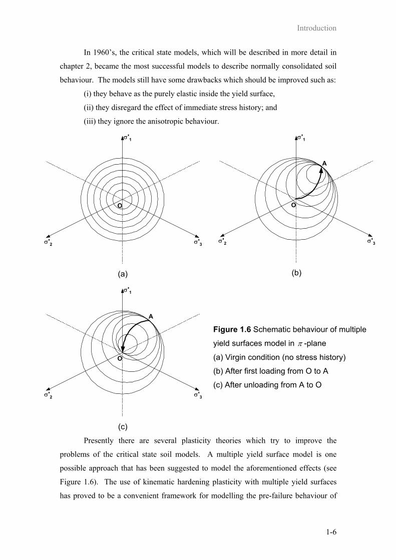
In 1960’s, the critical state models, which will be described in more detail in
chapter 2, became the most successful models to describe normally consolidated soil
behaviour. The models still have some drawbacks which should be improved such as:
(i) they behave as the purely elastic inside the yield surface,
(ii) they disregard the effect of immediate stress history; and
(iii) they ignore the anisotropic behaviour.
σ'1
σ'3σ'2
O
(a)
σ'1
σ'3σ'2
A
O
(b)
σ'1
σ'3σ'2
A
O
(c)
Figure 1.6 Schematic behaviour of multiple
yield surfaces model in π -plane
(a) Virgin condition (no stress history)
(b) After first loading from O to A
(c) After unloading from A to O
Presently there are several plasticity theories which try to improve the
problems of the critical state soil models. A multiple yield surface model is one
possible approach that has been suggested to model the aforementioned effects (see
Figure 1.6). The use of kinematic hardening plasticity with multiple yield surfaces
has proved to be a convenient framework for modelling the pre-failure behaviour of
Introduction
1-7
soils. This is because it can give a gradual change in stiffness, as more surfaces can
be used to increase the smoothness of the change. Furthermore, it is capable of
describing the effects of the immediate past history as well. The improvement of
anisotropic behaviour can be further included in the model.
1.3 Research objectives and structure of the thesis
Many plasticity theories are used and combined together to predict the stress-
strain response of soil in the overconsolidated state. The new constitutive model for
soil currently being developed is the multi yield surface type of model. Chapter 2
presents the background of constitutive soil models. Three examples of recently
developed soil models are illustrated; moreover, the model predictions and
comparisons are addressed in chapter 2.
A new development of a soil model based on thermomechanics is introduced
in chapter 3. The constitutive formulations in this chapter are developed based on the
modified Cam-clay model, which are presented in triaxial stress-strain parameters.
The incremental stress-strain calculation algorithms based on both rate-independence
and rate-dependence are presented in chapter 3.
Chapter 4 illustrates the experimental data from Bangkok clay, carried out by
Asian Institute of Technology (AIT) and Chulalongkorn University in Thailand. The
geological background for Bangkok clay and the testing programmes are stated here.
Prediction series of triaxial tests with the soil models are illustrated in chapter 5.
Comparisons between predictions and the experimental data from Bangkok clay are
also shown in chapter 5.
Chapter 6 explains the translation of the soil models from the triaxial stress-
strain parameters to generalised stress-strain parameters. The two-dimensional soil
models are implemented into the finite element program as new material subroutines.
A series of tests, which simulate the triaxial condition to test the new subroutines, are
carried out and presented in chapter 6. Two demonstrations using the models are
described in chapter 7. The comparisons between the analysis result and monitoring
data are also described in this chapter.
Finally, the conclusions on the development of new soil models are discussed
in chapter 8. Developments for future research are stated in this last chapter.

Constitutive model for soil
2-1
Chapter 2
Constitutive model for soil
A simple elastic theory is used to model the basic features of the stress-strain
behaviour of soils in routine engineering. An example is the calculation of final
settlement of a rigid foundation, in which a single parameter for soil stiffness or
flexibility (such as the coefficient of volume change, mv) will be sufficient to provide
the solution. However, additional predictions such as profiles of surface and
subsurface settlement, horizontal and vertical movements and soil-structure
interaction, require a relatively complex calculation and will usually need non-linear
stress-strain theory.
2.1 Constitutive models for soil
A general constitutive soil model can be written in the following form:
( )dtdFd ,σε = (2.1)
Note that σd and dt represent changes in effective stresses (not total stresses as in
other material models such as models for steel and concrete) and time respectively.
However, most soil models have been developed from the results of laboratory tests
with axi-symmetry condition (for example triaxial and oedometer tests).
Consequently, and for simplicity, the Cambridge parameters for stress and strain are
used to describe the stress-strain behaviour:
( ) ( )
( ) ( )3
2;2
;3
2
rasrav
rara qp
εεεεεε
σσσσ
−=+=
−=+
= (2.2)
where the subscripts a and r refer to axial and radial directions. The parameters p and
vε are mean effective stress and volumetric strain, whereas q and sε are deviatoric
stress and shear strain respectively. These parameters are related to the bulk modulus
K and shear modulus G by
sv d
dqG
d
dpK
εε== 3; (2.3)

Constitutive model for soil
2-2
Note that the multiplier 3 is needed to ensure that G corresponds to the general
definition used in solid mechanics. Graham and Houlsby (1983) introduce a general
constitutive equation for elastic anisotropic soil as
⋅
=
s
v
d
d
GJ
JK
dq
dp
εε
*
*
3 (2.4)
where J results in cross-coupling between shear and volumetric behaviour. In the
case of naturally deposited soil, the stiffness depends on mode of deposition and its
stress history. The superscript * is introduced to distinguish the anisotropic modulus
from the isotropic modulus.
For a material which is elastic and isotropic, shear and volumetric stiffness are
decoupled, that is, 0=J . The bulk modulus and shear modulus become elastic
following Hooke’s law, and the elastic constitutive equation can be written in the
form:
⋅
=
dq
dp
G
K
d
des
ev
310
01
εε
(2.5)
where GK , are elastic bulk modulus and elastic shear modulus respectively. Note
that the elastic parameters can also be defined in the term of Young’s modulus (E)
and Poisson’s ratio (υ ) by the relations ( )υ+⋅=
12
EG and ( )υ213 −⋅
=E
K .
2.2 Classical soil models
Many early developments of soil modelling are often referred to collectively
as Critical State Soil Mechanics (CSSM), introduced by Schofield and Wroth (1968).
CSSM combines three well-known concepts: the critical state line, normalisation with
respect to pre-consolidation pressure, and the state boundary surface (SBS). Based on
the critical state concept, a complete mathematical model of soil behaviour was
created by Roscoe, et al. (1963) and called Cam-clay model. The original Cam-clay
model developed for normally overconsolidated clay assumes that the energy is only
dissipated due to plastic shear distortion. Roscoe and Burland (1968) subsequently
developed the modified Cam-clay model (MCC), which considers both plastic
volumetric strain and plastic shear distortion in the formulation of the energy
dissipation equation.

Constitutive model for soil
2-3
The shape of modified Cam-clay yield locus is assumed to be elliptical, as
shown in Figure 2.1(a). The equation of the yield locus is:
02
22 =−+= cpp
M
qpy (2.6)
Making use of the state boundary surface as a yield surface and combining this with
an associated flow rule, the constitutive equation of modified Cam-clay can be
derived. The constitutive equation for plastic response may be expressed as:
( )( )( )
( )( )
( )( )
( )( )
⋅
+−−
+−
+−
++−−
=
dq
dp
GqpMv
pq
qpMv
qqpMv
q
pvqpMpv
qpM
d
d
s
v
3
142
2
444
2
222
222222
222
κλκλ
κλκκλ
εε
(2.7)
where v is a specific volume defined by ev +=1 , e is a void ratio, pc is the measure
of size of the yield surface which depends on the stress history, and M, λ, as well as κ
are the soil parameters that define the state boundary surface as shown in Figure 2.1.
(Note that the elastic bulk modulus for the MCC model is defined as:κpv
K = ) Thus,
the complete description of the model requires five parameters to specify the shape
and size of the yield locus at a given pressure and specific volume, as well as the
elastic properties of the material.
p
qM
pc
MCC yield surface
CSL
(a)
λ
κ
CSL
IsotropicNCL
SwellingLine
ln p
v
Pc
(b)
Figure 2.1 (a) Yield locus of Modified Cam-clay model; (b) Critical state soil parameters definition
The basic critical state model is particularly successful in describing the
principal features of soft clay behaviour. The model provides good predictions of
volumetric strain for normally consolidated soils subjected to isotropic consolidation.

Constitutive model for soil
2-4
However, it also has disadvantages. It does not describe anisotropic consolidation
conditions because the shape of the modified Cam-clay yield surface is symmetric
about the p-axis. It also gives poor predictions for heavily overconsolidated clay, in
particular for shear strains, since it assumes purely elastic and reversible inside state
boundary surface.
2.3 Development in soil models
In order to represent more realistic soil behaviour in a model, it is necessary to
introduce plasticity within the SBS. To date, several approaches have been proposed.
There are two main ideas that are often used to introduce plastic strain inside the SBS.
The first involves mapping the stress inside the SBS to an image point on an extra
surface usually known as the bounding surface. The plastic behaviour is obtained by
relating the stress and the image points by means of the hardening rule. Examples are
the bounding surface model by Dafalias and Herrmann (1982), the Hashiguchi model
by Hashiguchi (1985); and the MIT-E3 model by Whittle (1993).
The other idea is to introduce multiple yield surfaces to give a smoother
transition between elastic and plastic behaviour. This idea can also describe the effect
of the recent past history. Illustrations of this idea include the multiple nested yield
surface by Mroz et al. (1978), multiple surface model by Prevost (1978); and the
continuous hyperplasticity model by Einav, Puzrin and Houlsby (2001).
2.3.1 The bounding surface concept
In the original bounding surface model by Dafalias and Herrmann (1982),
there is a ‘radial mapping rule’, in which each stress state inside the SBS is mapped to
a corresponding image point on the bounding surface. This idea can be applied to a
soil model as shown in Figure 2.2(a). The SBS is defined as the MCC yield surface
and a radial mapping rule is adopted to define the image stress ( )*σ from the current
stress state ( )σ .
A smooth transition between elastic and plastic behaviours is obtained by
means of the hardening rule. The hardening rule can be written in the form:
Constitutive model for soil
2-5
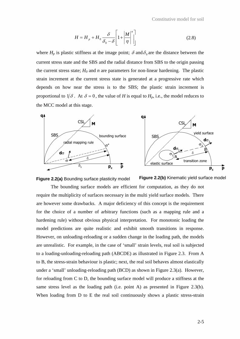
+
−+=
n
p
MHHH
ηδδδ
10
0 (2.8)
where Hp is plastic stiffness at the image point; δ and 0δ are the distance between the
current stress state and the SBS and the radial distance from SBS to the origin passing
the current stress state; H0 and n are parameters for non-linear hardening. The plastic
strain increment at the current stress state is generated at a progressive rate which
depends on how near the stress is to the SBS; the plastic strain increment is
proportional to δ1 . At 0=δ , the value of H is equal to Hp, i.e., the model reduces to
the MCC model at this stage.
M
p
q
pc
CSL
SBS
dσδ
δ0
σ∗
σ
radial mapping rule
bounding surface
Figure 2.2(a) Bounding surface plasticity model
q
M
ppc
CSL
SBS
dσ1δσ1
σ2
dσ2
elastic surfacetransition zone
yield surface
A
B
Figure 2.2(b) Kinematic yield surface model
The bounding surface models are efficient for computation, as they do not
require the multiplicity of surfaces necessary in the multi yield surface models. There
are however some drawbacks. A major deficiency of this concept is the requirement
for the choice of a number of arbitrary functions (such as a mapping rule and a
hardening rule) without obvious physical interpretation. For monotonic loading the
model predictions are quite realistic and exhibit smooth transitions in response.
However, on unloading-reloading or a sudden change in the loading path, the models
are unrealistic. For example, in the case of ‘small’ strain levels, real soil is subjected
to a loading-unloading-reloading path (ABCDE) as illustrated in Figure 2.3. From A
to B, the stress-strain behaviour is plastic; next, the real soil behaves almost elastically
under a ‘small’ unloading-reloading path (BCD) as shown in Figure 2.3(a). However,
for reloading from C to D, the bounding surface model will produce a stiffness at the
same stress level as the loading path (i.e. point A) as presented in Figure 2.3(b).
When loading from D to E the real soil continuously shows a plastic stress-strain
Constitutive model for soil
2-6
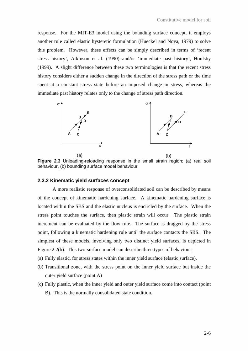
response. For the MIT-E3 model using the bounding surface concept, it employs
another rule called elastic hysteretic formulation (Hueckel and Nova, 1979) to solve
this problem. However, these effects can be simply described in terms of ‘recent
stress history’, Atkinson et al. (1990) and/or ‘immediate past history’, Houlsby
(1999). A slight difference between these two terminologies is that the recent stress
history considers either a sudden change in the direction of the stress path or the time
spent at a constant stress state before an imposed change in stress, whereas the
immediate past history relates only to the change of stress path direction.
σ
ε
A
B
C
D
E
(a)
σ
ε
A
B
C
D
E
(b)
Figure 2.3 Unloading-reloading response in the small strain region; (a) real soil behaviour, (b) bounding surface model behaviour
2.3.2 Kinematic yield surfaces concept
A more realistic response of overconsolidated soil can be described by means
of the concept of kinematic hardening surface. A kinematic hardening surface is
located within the SBS and the elastic nucleus is encircled by the surface. When the
stress point touches the surface, then plastic strain will occur. The plastic strain
increment can be evaluated by the flow rule. The surface is dragged by the stress
point, following a kinematic hardening rule until the surface contacts the SBS. The
simplest of these models, involving only two distinct yield surfaces, is depicted in
Figure 2.2(b). This two-surface model can describe three types of behaviour:
(a) Fully elastic, for stress states within the inner yield surface (elastic surface).
(b) Transitional zone, with the stress point on the inner yield surface but inside the
outer yield surface (point A)
(c) Fully plastic, when the inner yield and outer yield surface come into contact (point
B). This is the normally consolidated state condition.

Constitutive model for soil
2-7
The original idea of the kinematic hardening model was introduced separately
by Mroz (1967) and by Iwan (1967). Subsequently, the model has been extended to
multiple surfaces models by Prevost (1978). The best known of this is the multiple
“nested” yield surfaces model by Mroz et al. (1982). The multiple “nested” surfaces
model is based on the assumption that the yield surfaces do not overlap. In some
models overlapping is allowed, although this may occur only rarely.
The multiple yield surface models can successfully explain the effect of
immediate past history. However, there are again some disadvantages. Firstly, the
multiple surfaces model requires a considerable amount of calculation. This problem
can be reduced by using a rate-dependent algorithm, which will be addressed later.
Secondly, the multiple surfaces model requires a large number of hardening
parameters. This problem can be eliminated by introducing a function to replace a
large number of kinematic parameters.
2.4 Some recently developed soil models
This section will present some selected recent developments of constitutive
models for soil. Based on the two different approaches for plasticity inside the SBS,
the present research on constitutive models can be categorised into two groups as
already described in the previous section. However, there are some models which
merge the two ideas together and end up with somewhat complicated mathematical
expressions, which are practicable. The following will explain the developments of
some selected soil models which are a kinematic hardening model (Wood, 1995),
three-surface kinematic hardening model (Atkinson and Stallebrass, 1991) and the
MIT-E3 model (Whittle, 1993).
The first two models based on the kinematic hardening concept are selected to
present here. Both models are modified from an original ‘bubble’ model (Al Tabbaa
and Wood, 1989) to improve the transition zone between elastic behaviour and
elastoplastic behaviour. The parametric study for the kinematic hardening model
(Wood 1995) was done by Rouainia and Wood (2000) for Norrkoping clay. On the
other hand, the three-surface kinematic hardening model (Atkinson and Stallebrass,
1991) was laboratory validated by using a centrifuge model foundation test at City
University and also numerically implemented into a Finite Element analysis
(Stallebrass and Taylor, 1997).
Constitutive model for soil
2-8
The MIT-E3 is the well known example based on the bounding surface
concept. The parametric studies for MIT-E3 model were done by Whittle (1993) for
Boston blue clay at MIT and Zdravkovic et al.(2001) for silt at Imperial College by
using special equipment such as resonant column and large hollow cylindrical
apparatus respectively.
2.4.1 A kinematic hardening model (Wood, 1995)
The kinematic hardening framework was applied to the MCC model to
describe the behaviour of overconsolidated clay in a ‘bubble’ model, Al Tabbaa and
Wood (1989). The underlying assumption is that soil ‘structure’ is seen as a
strengthening contribution which is progressively removed by plastic strain. A
‘bubble’, hypothetically treated as a kinematically hardening yield surface, can
describe small strain stiffness, degradation of stiffness with strain for
overconsolidated clays and hysteretic behaviour due to the immediate stress history.
In this model, a ‘structure surface’ is introduced to control the process of
‘destructuration’ through its interaction with the bubble, and this destructuration can
capture strain softening effects.
The model consists of three elliptical yield surfaces (Figure 2.4(a)). A
reference surface (rs) represents the intrinsic behaviour of the remoulded material. Its
equation is defined as follows:
( ) 202
22
0 pM
qpp =+−
θ
(2.9)
where (p0,0) is the centre of this surface (20
cpp = in the MCC model). The
parameter θM is the ratio of the semi-axes of the yield surface, as in the MCC model.
Taking into account an unsymmetrical critical state cone between compression and
extension, θM is further defined as: ( ) ( ) θθ 3sin11
2
⋅−−+=
mm
mMM , where θ is an
angle on the π-plane related to the second and third stress invariants (J2, J3), that is
62
33sin
6 2/32
31 πθπ≤
−=≤− −
J
J. For the triaxial compression case
6
πθ = , MM =θ ;

Constitutive model for soil
2-9
whereas in the triaxial extension case6
πθ −= , mMM =θ . Note that normally the m
value should be between 1 and 0.7 for certain technical reasons.
A bubble with centre (pα,qα) and the size R times the size of the rs represents
the boundary of elastic response and the bubble’s equation can be written in the form:
( ) ( ) 20
22
22 pR
M
qqpp =
−+−
θ
αα (2.10)
A structure surface (ss) with size r times the size of the rs takes the place of the outer
yield surface, or can be thought of as a bounding surface. The ss controls the process
of destructuration, with its mathematical equation given by:
( ) ( )( ) 20
22
2002
0
1pr
M
prqrpp =
−−+−
θ
η (2.11)
where 0η is a dimensionless shear stress controlling the soil structure. The above
equation indicates that both the size and location of the ss are affected by the process
of destructuration through the variable r. Note that the centre of the ss is
( )( )000 1, prrp η⋅− .
The process of destructuration is controlled by the quantity r, which is
assumed to be a monotonic decreasing function of the plastic strain. A simple
exponential destructuration is then introduced as an example:
−−
−+=**0 exp)1(1
κλε dk
rr (2.12)
where r0 is the initial value of r (the initial degree of structure) probably related to the
sensitivity of the soil, and a general destructuration strain, dε , is defined as
( ) 221 p
sp
vd AddAd εεε +−= . The quantity ddε increases whenever plastic strain
pvdε or p
sdε occurs; the parameter A controls the relative influence that volumetric
and distortion effects have in causing destructuration. For A = 1, the destructuration is
completely distortional, whereas for A = 0, the destructuration is fully volumetric. The
parameter k controls the rate of destructuration with strain, and *λ and *κ represent the
slope of the NCL and swelling lines in log v-log p space.
The elastic behaviour inside the bubble is assumed as behave as in the MCC
model, with the elastic strain increments as given in equation (2.5). The plastic
Constitutive model for soil
2-10
strains occur when the stress state lies on the surface of bubble. The plastic strain
increment vector is assumed to lie in the direction of outward normal to the bubble at
the current stress. For the kinematic yield surface it is assumed that the size
parameter R is constant but the reference pressure p0 will be varying. Therefore,
when a stress increment is applied, it will require the kinematic hardening bubble to
translate. Since the bubble and ss have the same shape, a conjugate stress state cσ can
be determined on the ss in the same geometric position as the current stress state on
the bubble:
( )
−=
−−
α
α
η q
p
R
r
pr
rpσσ c
00
0
1 (2.13)
It is assumed that translation of the centre of the bubble occurs along the line joining
the current stress state σ and the conjugate stress state cσ . This ensures that the
bubble may touch the ss but can never intersect it. The constitutive equation can be
written into the form given below.
( ) ( ) ( )
( ) ( ) ( )
⋅
−−−
−−−
−=
dq
dp
M
M
qqpp
M
qqpppp
WRppd
d
bbb
bbb
ps
pv
2
22
2
2
0
**
θθ
θκλεε
(2.14)
where
( ) ( ) ( ) ( )( )2
2
2
2
2
2
max
0 11
−+−−
−−
−+−
+−=
θ
αα
θ
αα
ψ
αM
qqAppA
r
rk
M
qqpp
b
b
Rp
BpppW
and B, ψ are soil constants controlling the contribution and rate of change of
hardening. The scalar quantity b is the dot product between the vector joining the
stress state on the bubble σ and the conjugate stress state cσ on the ss and the
outward normal vector to the bubble. Because all the yield surfaces are elliptical in
(p,q) space, the maximum value of bmax will occur when the bubble is touching the ss
at a point diametrically opposite to the conjugate stress state (Figure 2.4(b)).
The model uses both the concepts of a kinematic hardening yield surface and a
bounding surface. The elastic behaviour, when the stress state is inside the bubble,
can be described by means of the MCC model. The bubble kinematic yield surface

Constitutive model for soil
2-11
can be used to describe the immediate stress history at the small strain level relatively
well. However, due to the limitation of a single kinematic yield surface, the soil
behaviour under a complex applied load history (such as cyclic loading) cannot be
captured by the model. The introduction of the structure surface (or bounding
surface) with the destructuration parameters can model aspects of the ansiotropic and
strain softening behaviour by allowing the centre of the structure surface to move. All
of the surfaces are elliptic in shape similar to the MCC yield surface. The model also
modifies the value of semi-axis ratio of (M) by considering the asymmetry of the
critical state cone in compression and extension. The plastic behaviour of
overconsolidated clay can be described by a hardening rule using the bounding
surface concept which uses a geometric mapping rule. The two hardening parameters
are added in order to describe nonlinear plasticity behaviour.
M
p
qCSL
SBS
Structure surface, ss
Referencesurface, rs
Bubble
pα,qα
p0
rp0
Rp0
rp0 , (r-1)η0p0
(a)
p
q
bbmax
σcσ
σb
Structuresurface, ss
Bubble
η0
Referencesurface, rs
(b) Figure 2.4 (a) Elastic bubble, reference surface (rs), and structure surface (ss) for destructration model in triaxial space; (b) Conjugate stress ( cσ ) and corresponding
stress ( bσ ) on extreme bubble for definition of bmax, Wood (1995)
2.4.2 Three-surface kinematic hardening model (Atkinson and Stallebrass, 1991)
The three-surface kinematic hardening (3-SKH) soil model was formulated
specifically to simulate the behaviour of clays in overconsolidated states and during
early stages of loading. The model gives an improvement to the ‘bubble’ model of Al
Tabbaa and Wood (1989), so that the effect of immediate stress history and yield at
small strains or changes in the stresses can be modelled. The model is represented in
p-q space in Figure 2.5(a). It requires three yield surfaces: Modified Cam-clay SBS
(referred to as the bounding surface), and two nested kinematic surfaces (yield surface
Constitutive model for soil
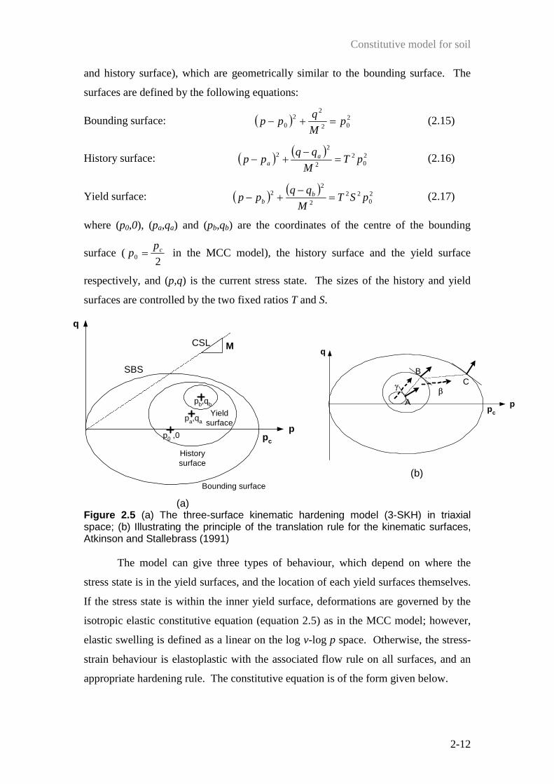
2-12
and history surface), which are geometrically similar to the bounding surface. The
surfaces are defined by the following equations:
Bounding surface: ( ) 202
22
0 pM
qpp =+− (2.15)
History surface: ( ) ( ) 20
22
22 pT
M
qqpp a
a =−
+− (2.16)
Yield surface: ( ) ( ) 20
222
22 pST
M
qqpp b
b =−
+− (2.17)
where (p0,0), (pa,qa) and (pb,qb) are the coordinates of the centre of the bounding
surface (20
cpp = in the MCC model), the history surface and the yield surface
respectively, and (p,q) is the current stress state. The sizes of the history and yield
surfaces are controlled by the two fixed ratios T and S.
M
p
q
CSL
SBS
Bounding surface
Historysurface
Yieldsurface
pa,qa
pb,qb
p0 ,0 pc
(a)
p
q
pc
A
BC
βγ
(b)
Figure 2.5 (a) The three-surface kinematic hardening model (3-SKH) in triaxial space; (b) Illustrating the principle of the translation rule for the kinematic surfaces, Atkinson and Stallebrass (1991) The model can give three types of behaviour, which depend on where the
stress state is in the yield surfaces, and the location of each yield surfaces themselves.
If the stress state is within the inner yield surface, deformations are governed by the
isotropic elastic constitutive equation (equation 2.5) as in the MCC model; however,
elastic swelling is defined as a linear on the log v-log p space. Otherwise, the stress-
strain behaviour is elastoplastic with the associated flow rule on all surfaces, and an
appropriate hardening rule. The constitutive equation is of the form given below.

Constitutive model for soil
2-13
( ) ( ) ( )
( ) ( ) ( )
⋅
−−−
−−−
=
dq
dp
M
M
qqpp
M
qqpppp
hd
d
bbb
bbb
ps
pv
2
22
2
2
1
εε
(2.18)
where h = h0 + H1 + H2 , and ( ) ( ) ( )
−+−
−−
=2**0
M
qqqppp
pph b
bb
κλ.
*λ and *κ represent the slope of the NCL and swelling lines in the log v-log p space.
The above equations can be reduced to the MCC constitutive equation when all the
surfaces are in contact (h = h0). Otherwise, the general case has to include H1 and H2
terms, which are functions of the position of the history and yield surfaces
respectively. The functions H1 and H2 have to be added to ensure that they will give a
smooth change in stiffness, so an exponent is introduced as a hardening modulus
parameter, ψ. The general hardening function can be finally expressed in the form:
( ) ( ) ( )
+
+
−
+−⋅−−
= 30
max2
2230
max1
12**
1p
b
bSp
b
b
M
qqqppppph b
bb
ψψ
κλ (2.19)
where b1 is the dot product of the normal vector at point B and vector β (the
movement vector from the point B on the history surface to the point C on the
bounding surface). b2 is the dot product of the normal vector at point A and vector γ
(the movement vector from the point A on the yield surface to the point B on the
history surface). These can be illustrated in Figure 2.5(b).
The model adds another kinematic hardening yield surface to improve the
variation of the elastoplastic stiffness; this make an improvement from the original
‘bubble’ model by Al Tabbaa and Wood (1989). The modifications on the effect of
recent stress history and yield at small strains are obtained by means of the two
kinematic and one outer yield surfaces with the same elliptical geometry. The size of
each surface is controlled by two fixed ratios (T, S). The model captures three types
of behaviour, depending on where the stress state is in the yield surfaces and the
location of each yield surfaces themselves. The elastic behaviour occurs, when the
stress state is inside the yield surface. The plastic behaviour of the overconsolidated
clay can be described by the kinematic hardening rule. The hardening exponent (ψ )
is adopted in order to explain the smooth transition of stiffness.

Constitutive model for soil
2-14
2.4.3 The MIT soil models (Whittle, 1993 and Pestana and Whittle, 1999)
Research at the Massachusetts Institute of Technology (MIT) has developed a
series of generalised rate independent models for clays based on the theory of
incremental linear elasto-plasticity. This model evolved from MIT-E1. Its key
features are an anisotropic yield surface, kinematic plasticity and strain softening
behaviour under undrained condition for normally consolidated clays. Subsequently,
the further developments on model, MIT-E3, describe the rate independent behaviour
of normally to moderately overconsolidated clays (OCR<8). The two additional
features incorporated into MIT-E3 are small strain nonlinear elasticity using a closed
hysteric loop and bounding surface plasticity.
The MIT-E3 model’s conceptual framework can be subdivided into three
components:
(a) an anisotropic yield surface with hardening rule and flow rule;
(b) a closed symmetric hysteresis loop; and
(c) a bounding surface plasticity formulation.
Table 2.1 Comparison between transformed variables for MIT-E3
Variables Generalised space Triaxial space
Effective stress ijσ ′ ( )qp,
Strain ijε ( )sv εε ,
Yield surface gradient ij
fσ ′∂∂ , where f is yield function
( )qp QQ , , where
pfQp ∂∂
= and qfQq ∂∂
=
Plasticity flow
direction ij
gσ ′∂∂ , where g is plastic
potential function
( )qp PP , , where pgPp ∂∂
=
and qgPq ∂∂
=
Anisotropic axis ijb ( )b,1
The anisotropic model always has to deal with all six components of the stress-strain
or some meaningful definitions. The constitutive relations have been presented in the

Constitutive model for soil
2-15
original paper in terms of generalised effective stresses. However, in order to be
equivalent to other models, the MIT-E3 model equation will be expressed in triaixal
stress-strain parameters. This will make the MIT-E3 model formulation slightly
different from the original work. For more detail see Potts and Zdravkovic (1999).
Table 2.1 presents a comparison between the transformed variables that are used in
the original paper and variables in the triaxial case.
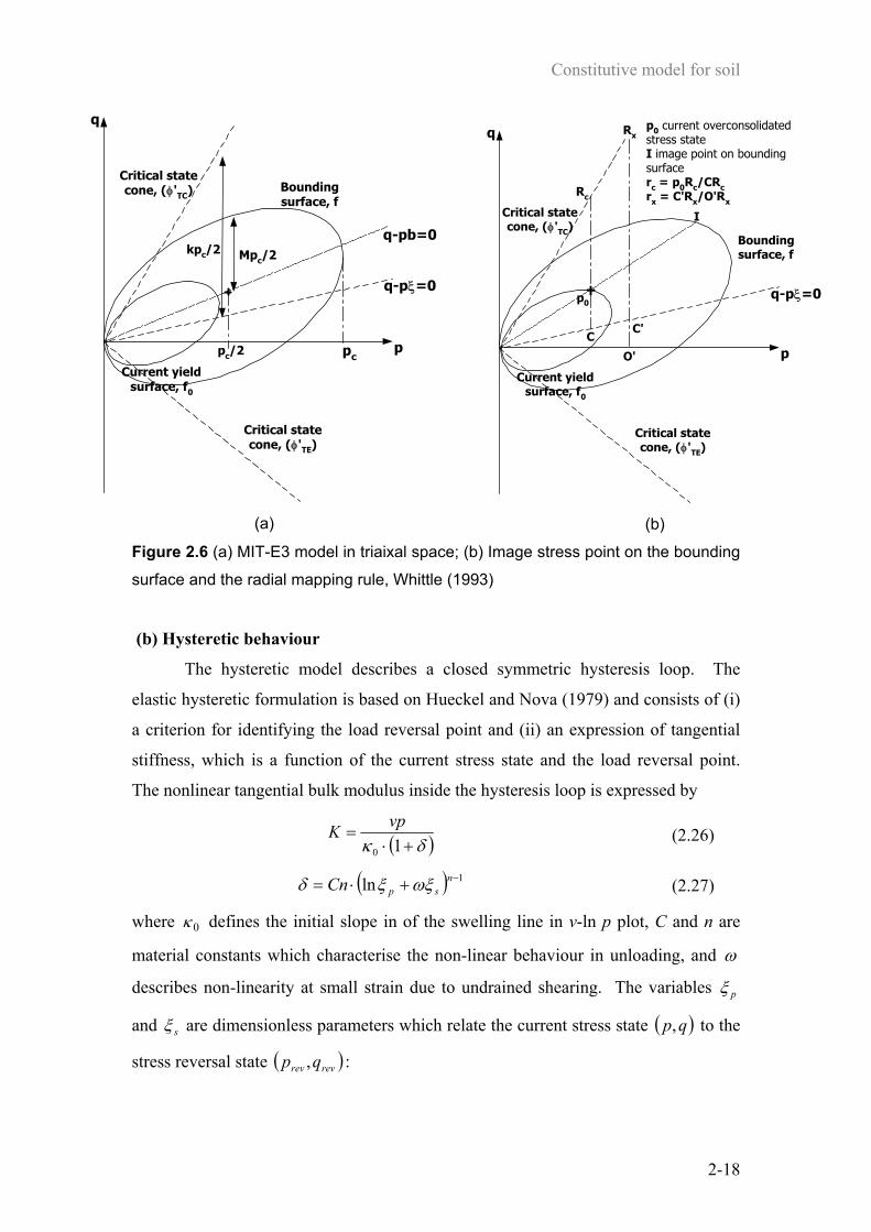
(a) An anisotropic yield surface
The yield function (Figure 2.6(a)) is assumed to be an anisotropic form of the
elliptical modified Cam-clay yield written in the form:
( ) ( ) 022 =−−⋅−= pppMbpqf c (2.20)
where b is the direction of the yield surface axis and M defines the ratio of the semi-
axes of the ellipsoid, which is slightly different from the critical state definition.
The failure criterion, at which critical state behaviour is exhibited, is defined
by an anisotropic conical surface:
( ) 0222 =−⋅−= pkpqh ξ (2.21)
where h describes two boundaries of the critical state cone in compression and
extension. Its axis of symmetry is on the direction ξ from p-axis, and a constant k
parameter defines the half range of critical state cone. These two parameters ( k,ξ )
can be fully defined by the friction angles measured in triaxial compression and
extension tests ( TETC φφ ′′ , based on Mohr-Coulomb’s failure criteria):
( )ec CC −=21ξ ; ( )ec CCk +=
21
where TC
TCcC φ
φ′−′
=sin3
sin632 ;
TE
TEeC φ
φ′+′
=sin3
sin632 .
Note that the direction of anisotropy of the yield surface (b) does not generally
coincide with the direction of anisotropy of the critical state cone (ξ ) as shown in
Figure 2.6(a).
Flow rule
The model uses a non-associated flow rule with the flow direction defined as:
Constitutive model for soil
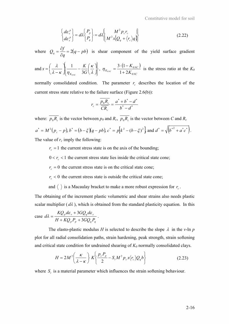
2-16
{ }
+=
=
qrQxMrpM
dPP
ddd
cq
cc
q
pps
pv
2
2
λλεε
(2.22)
where ( )pbqqfQq −=∂∂
= 2 is shear component of the yield surface gradient
and
−
−=
λκ
ηκλλ
GKx
NCK 31
0
, ( )
NC
NCK K
KNC
0
0
2113
0 +−⋅
=η is the stress ratio at the K0
normally consolidated condition. The parameter cr describes the location of the
current stress state relative to the failure surface (Figure 2.6(b)):
**
***0
dbdba
CRRp
rc
cc −
−+==
where: cRp0 is the vector between p0 and Rc, cRp0 is the vector between C and Rc
( ) ( )( ) [ ] ( )**2**22**2* and,)(,, cabdbkpcpbqbbppMa c +=−−=−−=−= ξξ .
The value of rc imply the following:
1=cr the current stress state is on the axis of the bounding;
10 << cr the current stress state lies inside the critical state cone;
0=cr the current stress state is on the critical state cone;
0<cr the current stress state is outside the critical state cone;
and is a Macaulay bracket to make a more robust expression for cr .
The obtaining of the increment plastic volumetric and shear strains also needs plastic
scalar multiplier ( λd ), which is obtained from the standard plasticity equation. In this
case qqpp
sqvp
PGQPKQHdGQdKQ
d3
3++
+=
εελ .
The elasto-plastic modulus H is selected to describe the slope λ in the v-ln p
plot for all radial consolidation paths, strain hardening, peak strength, strain softening
and critical state condition for undrained shearing of K0 normally consolidated clays.
−⋅
−= bQrxpMS
PpKMH qcct
pc 22
22
κλκ (2.23)
where tS is a material parameter which influences the strain softening behaviour.

Constitutive model for soil
2-17
Hardening rule
The model assumes two hardening rules to describe changes in size and
orientation of the yield surface respectively:
pv
c
c dpdp
εζ ⋅= (2.24)
( ) pvx
c
dpbqrp
db ε−Ψ
= 02 (2.25)
where ζ is a scalar, obtained from the consistency requirement ( )0=df . In this
case: ( )
−
Ψ−⋅=c
cx
pcc pppp
rPH
pMp212
02ζ , with 0Ψ being a material constant
controlling the rate of rotation of the yield surface. xr is a relative ratio between
orientation of the yield surface and the critical state cone, which is graphically
illustrated in Figure 2.6(b) and is defined as:
kbk
ROCR
rx
xx
ξ−−=
′=
The value of rx imply the following:
1=xr the axis of yield surface coincides with the axis of the critical state cone;
10 << xr the axis of yield surface lies inside the critical state cone;
0=xr the axis of yield surface is on the critical state cone;
0<xr the axis of yield surface is outside the critical state cone.
The equation (2.25) describes rotational hardening of the yield surface and hence
controls the rate of change of anisotropy of the clay. The variable xr is controlled by
the degree of anisotropy: 10 <≤ xr (If 1=xr , the clay is an isotropic material). From
the fact that the axes of anisotropy does not rotate outside the critical state cone, thus
Macaulay bracket is introduced in the expression for xr .
Constitutive model for soil
2-18
q
ppcpc/2
Mpc/2
q-pb=0
q-pξ=0
Boundingsurface, f
Current yieldsurface, f0
Critical statecone, (φ'TC)
Critical statecone, (φ'TE)
kpc/2
(a)
q
p
Rx
q-pξ=0p0
Boundingsurface, f
Current yieldsurface, f0
Critical statecone, (φ'TC)
Critical statecone, (φ'TE)
I
Rc
O'
C
p0 current overconsolidatedstress stateI image point on boundingsurfacerc = p0Rc/CRcrx = C'Rx/O'Rx
C'
(b)
Figure 2.6 (a) MIT-E3 model in triaixal space; (b) Image stress point on the bounding
surface and the radial mapping rule, Whittle (1993)
(b) Hysteretic behaviour
The hysteretic model describes a closed symmetric hysteresis loop. The
elastic hysteretic formulation is based on Hueckel and Nova (1979) and consists of (i)
a criterion for identifying the load reversal point and (ii) an expression of tangential
stiffness, which is a function of the current stress state and the load reversal point.
The nonlinear tangential bulk modulus inside the hysteresis loop is expressed by
( )δκ +⋅=
10
vpK (2.26)
( ) 1ln −+⋅= nspCn ωξξδ (2.27)
where 0κ defines the initial slope in of the swelling line in v-ln p plot, C and n are
material constants which characterise the non-linear behaviour in unloading, and ω
describes non-linearity at small strain due to undrained shearing. The variables pξ
and sξ are dimensionless parameters which relate the current stress state ( )qp, to the
stress reversal state ( )revrev qp , :

Constitutive model for soil
2-19
>>
=pppp
pppp
revrev
revrevp for
forξ (2.28)
revq ηηξ −= (2.29)
where pq=η is the stress ratio. The major assumption of the perfectly hysteretic
model is that the strains are fully recovered in a stress cycle. A further assumption is
that there is uncoupling between volumetric and shear behaviour in the perfectly
hysteretic model. Therefore, the elastic shear modulus (G) can be described by the
elastic relation, in which a constant Poisson’s ratio (or K/G constant) is used.
Another feature of this formulation is that the hysteretic behaviour is only a
function of the last load reversal point and maintain no memory of any previous
loading history. The definition of the load reversal point is achieved by introducing a
scalar strain amplitude parameter which describes the strain history from the
immediate stress reversal point as follows:
=−≠−
=0if0if
vrevss
vrevvv
εεεεεε
χ&
& (2.30a)
A load reversal point then occurs when the magnitude of χ reduces, i.e. 0<∆χ .
However, as the condition above is difficult to implement in an analysis, a more
robust expression is presented by Potts and Zdravkovic (1999):
( ) ( )22revssrevvv εεεεχ −+−= (2.30b)
(c) Bounding surface plasticity
In the case of normally consolidated clay, the bounding surface is described by
the yield function; whereas, for overconsolidated clay, a radial mapping rule defines a
unique image point on the bounding surface (Figure 2.6(b)). Plastic behaviour at the
current stress state (p0) is linked to the plastic behaviour at the image point I. The
plastic strain increments at p0 depend on the loading condition defined as:
<≥
=+Unloading
Loading
00
3 sqvp dGQdKQ εε (2.31)
where pQ and qQ are the yield surface gradients at the image stress point in the
volumetric and deviatoric directions respectively.

Constitutive model for soil
2-20
The MIT-E3 model assumes separate mapping rules for the elasto-plastic
modulus H and flow direction Pp, Ps at the current stress state p0 inside the bounding
surface. The flow direction and modulus are given in the forms:
⋅−
=
Iq
pIp
q
p
PgPP
PP γ
10 (2.32)
20 gHHH I ⋅+= (2.33)
where { }IqIccp QrpMP η+= 2
0,
icc
cc
pppp
g0
01 −
−= ,
icc
cc
pppp
g00
02 −
−= , and
( )IpIpcc PhQppvH 0
00 2
−=κ
; in which 0cp and icp 0 are the reference pressure of the
yield surface at the current stress state p0 and at the first yield, and h and γ are
dimensionless input parameters.
The MIT soil models have been developed based on experimental data,
especially that on Boston Blue clay. The conceptual framework encompasses three
concepts:
(a) K0 normally consolidated yield surface, which allows yield surface distortion;
(b) a perfectly hysteretic model, which give a smooth changes of tangential
stiffness during unloading; and
(c) a bounding surface model with the radial mapping rule, which describes the
plastic behaviour inside yield surface by using the non-linear hardening rule.
2.5 Evaluation and Prediction of Models In general, after the development of the model formulation, a parametric study
is carried out mostly by an evaluation of model against laboratory data especially
triaxial test. The simulation of a stress path triaxial test is carried out by using a
computer program which models the test as a single element. A set of model
parameters for any particular soil are obtained by using the procedure outlined above
excepted some special model parameters which may require sophisticated apparatus
such as resonant column and large hollow cylinder.

Constitutive model for soil
2-21
2.5.1 A kinematic hardening model (Rouainia and Wood, 2000) The kinematic hardening model has been specifically tested for its ability to
reproduce a series of triaxial test results for Norrkoping clay from Sweden (Rouainia
and Wood, 2000). The thirteen model parameters have been estimated by using an
automatic optimization procedure. The assumption that all samples from the same
depth have the same initial conditions such as stress state, location of yield surface
and structure surface is made. However, the value of 00** and,,, ηλκ r have been
varied with depth in order to improve the match for the test concerned. The resulting
set of model parameters, which has been used for matching the data at 5m depth, is
shown in Table 2.2.
Table 2.2 Kinematic hardening model parameters for Norrkoping clay at depth
5m (After Rouainia and Wood, 2000) Symbols Physical meaning Value
*κ Slope of swelling line in ln v–ln p plot 0.0297
υ Poissons’s ratio 0.22 *λ Slope of NCL in ln v–ln p plot 0.252
M Critical state stress ratio 1.35
m Ratio of extension and compression strength 0.85
R Ratio of size of bubble and reference surface 0.145
bmax Stiffness interpolation parameter 1.980 ψ Stiffness interpolation exponent 1.547
k Destructuration parameter 4.16
A Destructuration strain parameter 0.494
pc0 Initial centre of reference surface 13.28
r0 Initial degree of structure 1.75
0η Anisotropy of initial structure 0.50
The simulations of the consolidation procedure for all tests follow the stress
path in Figure 2.7. The optimization has been done using a K0-consolidated undrained
compression and extension triaxial test (CK0UC and CK0UE) with approximately the
same effective stresses at the starting point (Figure 2.8). Other predictions based on
the optimized parameters have been carried out, which are

Constitutive model for soil
2-22
(i) isotropic normally consolidated undrained compression tests with four
different pressures of 40, 50, 58 and 100 kPa (Figure 2.9);
(ii) anisotropic normally consolidated undrained compression tests with four
different initial stresses (Figure 2.10); and
(iii) isotropic overconsolidated undrained compression tests with three different
overconsolidation ratios of 2, 5 and 9 (Figure 2.11).
Figure 2.7 Stress path during consolidation procedure
( i = in-situ stress state; s = stress state at start of shearing);
(a) isotropic starting stress, (b) anisotropic starting stress,
Rouainia and Wood (2000)
It is not surprising that the normally consolidated undrained compression tests
(Figure 2.8 and 2.9) can be predicted well by the kinematic hardening model. This is
because the outer surface of the kinematic hardening model uses the MCC model
yield surface that generally gives a good prediction for the normally consolidation
clay. An improvement of the M value offers a slightly better prediction for
anisotropic normally consolidated undrained compression tests. This model gives
relatively accurate predictions for the overconsolidated sample, especially for the
stress path direction (Figure 2.10). The model can also describe the softening
behaviour due to the destructuration process (that allows the yield surface to relocate)
as shown in Figure 2.10. When actually presenting the tests results, however,
Rouainia and Wood changed some parameters including A, B,ψ , k and r0 for two
drained compression tests. It seems unreasonable to tune some parameters to offer a
better prediction of drained shear behaviour.
However, the simulation still requires at least another set of experimental
triaixal extension tests. The two predictions of drained shear tests are not enough to
make a conclusion. Moreover, there is still no evidence on hysteretic behaviour,

Constitutive model for soil
2-23
especially the effects of immediate stress history on the unload-reload stress-strain
response.
Figure 2.8 K0-consolidated undrained triaxial
compression and extension tests and KH-
model predictions for Norrkoping Clay,
Rouainia and Wood (2000)
Figure 2.9 Isotropic normally consolidated
undrained triaxial compression tests varied
pressures of 40, 50, 58 and 100 kPa and KH-
model prediction for Norrkoping Clay,
Rouainia and Wood (2000)
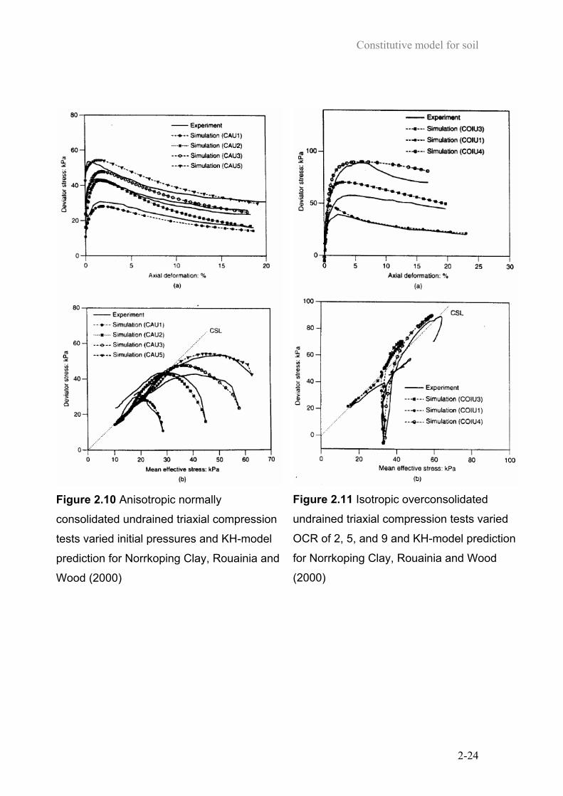
Constitutive model for soil
2-24
Figure 2.10 Anisotropic normally
consolidated undrained triaxial compression
tests varied initial pressures and KH-model
prediction for Norrkoping Clay, Rouainia and
Wood (2000)
Figure 2.11 Isotropic overconsolidated
undrained triaxial compression tests varied
OCR of 2, 5, and 9 and KH-model prediction
for Norrkoping Clay, Rouainia and Wood
(2000)

Constitutive model for soil
2-25
2.5.2 Three-surface kinematic hardening model (Stallebrass and Taylor,
1997) A set of 3-SKH model parameters is obtained for comparison with the
experimental data from Speswhite kaolin as shown in Table 2.3 (Stallebrass and
Taylor, 1997). All eight parameters in the model are assumed to be constant, except
the elastic shear modulus (G ), which varies with p and OCR according to the power
function. Five of the parameters ( cseandGM ,,,, ** λκ ) carry the same meanings
and significance as previously defined in the MCC model. T and S can be evaluated
from two sets of isotropic consolidation stress paths (Figure 2.12(a)):
(i) a stress path after swelling from half of the maximum stress history (O-B-A); and
(ii) a stress path after one cycle of stress reversal (O-B-A-B-A).
The typical plots of secant bulk modulus ( cK ) against p can be used to estimate T
and S values (Figure 2.12(b)). However, the exponent for the hardening modulus, ψ
is the only parameter that cannot be obtained directly from the experimental data; it
has to be derived from parametric studies.
Table 2.3 3-SKH model parameter for Speswhite kaolin (After Stallebrass,
1990) Symbols Physical meaning Value
*κ Slope of swelling line in ln v–ln p plot 0.005
*λ Slope of NCL in ln v–ln p plot 0.073
M Critical state stress ratio 0.89
T Ratio of size of history to bounding surface 0.25
S Ratio of size of yield surface to history surface 0.08 ψ Exponent in hardening modulus 2.5
ecs Void ratio of isotropically normally
consolidated soil at reference pressure pr=1kPa 1.994
G Elastic shear modulus 60000*
*Calculate from 2.065.0
1964 OCRppG
r
⋅
=

Constitutive model for soil
2-26
Figure 2.12 Sketch showing (a) isotropic stress
path required to determine values for
parameters T and S; (b) typical stiffness plots
from T and S can be estimated, Atkinson, et al.
(1991)
Figure 2.14 Comparison between stiffness data
computed from a single element simulation and
measured data, Atkinson, et al. (1991)
Figure 2.13 Typical stress path showing the recent stress history (AO) and its
sudden change of direction; (a) Anticlockwise direction (negative θ ), (b) Clockwise
direction (positive θ ), Atkinson, et al. (1991)

Constitutive model for soil
2-27
Figure 2.15 Cycle of loading during test, pini = 300 kPa,
pmax = 720 kPa: comparison between predicted and
measured stress-strain response, Atkinson, et al. (1991)
A study of the effect of recent stress history has been experimentally carried
out by Atkinson et al. (1991), who use test procedures as illustrated in Figure 2.13.
The simulations of tests have been numerically reproduced by following the same
stress paths. Figure 2.14 shows a comparison between experimental secant shear
modulus data and the model predictions. A study of the hysteresis loop has been done
by means of unload-reload shear stress at constant p . The comparison between the
model prediction and experimental data is shown in Figure 2.15.
The 3-SKH model is developed with the purpose of describing the effect of
recent stress history. Therefore, the presented paper emphasises only this effect.
Although the 3-SKH model can explain the variation of shear modulus due to a
sudden change of stress path direction during shearing process, the curve is still not
smooth. This might be a result of the fact that number of the kinematic yield surfaces
is limited to only two. The 3-SKH model could show two sudden changes of
elastoplastic behaviour when the inner surface touches the outer surface. For the
hysteretic behaviour, the prediction of the unload-reload shear stress-strain shape is
correct. The magnitude still needs improvement nevertheless.
Constitutive model for soil
2-28
A yield surface shape that uses the elliptic modified Cam-clay yield surface
can explain the normally consolidated behaviour. The model still needs a proof of
anisotropic behaviour particularly on K0-consolidated undrained/drained compression
and extension tests.
2.5.3 The MIT-E3 model (Whittle et al., 1994)
The fifteen input parameters for the MIT-E3 model can be evaluated directly
or indirectly based on laboratory tests, as presented in Table 2.4. The parameters that
can be directly measured from standard laboratory tests are:
,0e ,0NCK ,GK ,, TETC φφ ′′ 0and κλ . The remaining input constants must be
determined from parametric studies:
(i) C, n are the parameters for the nonlinear in perfect hysteretic volumetric
response and h is the controlling parameter for the amount of irreversible
volumetric strain, which can be selected to match swelling curves from the CRS
consolidometer (Figure 2.16);
(ii) St and M are established from the K0-consolidated undrained shear
compression and extension (CK0UC and CK0UE) at OCR = 1.0, which control the
shape of the undrained path in both compression and extension (Figure 2.17);
(iii) γω and are nonlinear secant shear modulus at small strain level and shear-
induced pore pressure at large strain level during undrained shear condition
respectively, which can be measured from the secant modulus and excess pore
pressure; and
(iv) 0ψ controls the rate of change of the anisotropic direction (yield surface
rotation), which suggested the reasonable values between 75 to 200 based on the
parametric studies (Figure 2.18).
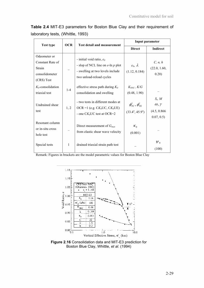
Constitutive model for soil
2-29
Table 2.4 MIT-E3 parameters for Boston Blue Clay and their requirement of
laboratory tests, (Whittle, 1993)
Input parameter Test type OCR Test detail and measurement
Direct Indirect
Odeometer or
Constant Rate of
Strain
consolidometer
(CRS) Test
_
- initial void ratio, e0
- slop of NCL line on e-ln p plot
- swelling at two levels include
two unload-reload cycles
e0, λ
(1.12, 0.184)
C, n, h
(22.0, 1.60,
0.20)
K0-consolidation
triaxial test 1-4
effective stress path during K0
consolidation and swelling
K0NC , K/G
(0.48, 1.90) _
Undrained shear
test 1, 2
- two tests in different modes at
OCR =1 (e.g. CK0UC, CK0UE)
- one CK0UC test at OCR=2
TETC φφ ′′ ,
(33.4o, 45.9o)
St, M γω,
(4.5, 0.866
0.07, 0.5)
Resonant column
or in-situ cross
hole test
_ Direct measurement of Gmax
from elastic shear wave velocity 0κ
(0.001) _
Special tests 1 drained triaxial strain path test _ 0ψ
(100)
Remark: Figures in brackets are the model parametric values for Boston Blue Clay
Figure 2.16 Consolidation data and MIT-E3 prediction for
Boston Blue Clay, Whittle, et al. (1994)

Constitutive model for soil
2-30
Figure 2.17 K0-consolidated undrained triaxial compression and extension shear data and
MIT-E3 prediction for Boston Blue Clay, Whittle, et al. (1994)
Figure 2.18 Parametric studies of 0ψ value and MIT-E3 prediction of
drain strain path triaxial test, Whittle, et al. (1994)

Constitutive model for soil
2-31
Figure 2.19 K0-consolidated undrained plan strain compression and extension shear data
varied OCR = 1-4 and MIT-E3 prediction for Boston Blue Clay, Whittle, et al. (1994)
The MIT-E3 model offers accurate predictions for Boston Blue Clay as shown
in Figures 2.16, 2.17 and 2.19. This is because the model contains many advantages
of theories such as the bounding surface theory (Dafalias and Herrmann, 1982), the
elastic hysteretic formulation (Hueckel and Nova, 1979) and the anisotropic yield
surface and critical state cone. In particular, the stress path of anisotropic
consolidated tests can be simulated by the MIT-E3 model as presented in Figures 2.17
and 2.19. Although the hysteresis loop can be reproduced by the MIT-E3 model, it is
controlled by the stress reversal point. This cannot be used to explain the complicated
unloading response; for instance the three different unloading paths from A to B in the
generalised stress space as illustrated in Figure 2.20. The elastic hysteretic
formulation (Hueckel and Nova, 1979) cannot be used to distinguish the responses
from these three different unloading paths because they are unloaded from the same
reversal stress point (i.e. point A).
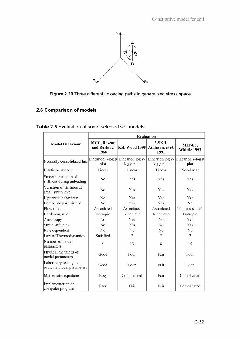
Constitutive model for soil
2-32
σ1
σ2 σ3
A
B
123
Figure 2.20 Three different unloading paths in generalised stress space
2.6 Comparison of models Table 2.5 Evaluation of some selected soil models
Evaluation
Model Behaviour MCC, Roscoe and Burland
1968 KH, Wood 1995
3-SKH, Atkinson, et al.
1991
MIT-E3, Whittle 1993
Normally consolidated line Linear on v-log pplot
Linear on log v-log p plot
Linear on log v-log p plot
Linear on v-log pplot
Elastic behaviour Linear Linear Linear Non-linear Smooth transition of stiffness during unloading No Yes Yes Yes
Variation of stiffness at small strain level No Yes Yes Yes
Hysteretic behaviour No Yes Yes Yes Immediate past history No Yes Yes No Flow rule Associated Associated Associated Non-associatedHardening rule Isotropic Kinematic Kinematic Isotropic Anisotropy No Yes No Yes Strain softening No Yes No Yes Rate dependent No No No No Law of Thermodynamics Satisfied ? ? ? Number of model parameters 5 13 8 15
Physical meanings of model parameters Good Poor Fair Poor
Laboratory testing to evaluate model parameters Good Poor Fair Poor
Mathematic equations Easy Complicated Fair Complicated
Implementation on computer program Easy Fair Fair Complicated

Constitutive model for soil
2-33
Each soil model described above tries to explain the behaviour of
overconsolidated soil with the aim of generating plastic behaviour inside the SBS
which could not be previously achieved by a conventional plasticity model. Of the
several frameworks of plasticity theory with mathematically sophisticated equations,
most are based on two different concepts: bounding surface models (Dafalias and
Herrmann, 1982) and kinematic hardening models (Mroz, 1967 and Iwan, 1967).
There are some advantages and disadvantages in relation to both concepts. The
models introduced previously are compared in Table 2.5. The author’s comments in
Table 2.5 present not only the facts but also the author’s views especially in the last
four lines. For instance physical meanings of model parameters: ‘good’ for the MCC
model means that the author is of the opinion that all the physical meanings of the
parameters are well defined; however, ‘poor’ for the MIT-E3 model refers to a lack of
clear definition for the physical meanings of some of the model parameters.
Table 2.6 Comparison of physical meaning of soil model parameters
Symbols Physical meaning of
parameter MCC, Roscoe and Burland
1968 KH, Wood 1995
3-SKH, Atkinson, et al.
1991
MIT-E3, Whittle 1993
Normally consolidated line λ,κ λ∗,κ∗ λ∗,κ∗ λ,κ0
Reference of yield surface pc p0 P0 pc (2α) Elastic parameter G* or ν G* (ν) G* K/G Critical state parameter M Mθ M M (c) Anisotropic parameters - m, η0 - K0NC, φ'TC, φ'TE Non-linear hardening parameter - B,ψ ψ h, γ, Ψ0
Non-linear at small strain - r0,A,k,ψ T,S,ψ C,n,ω
Parameters describe the effect of immediate history - R,r0 T,S -
Strain softening parameter - r0 - St
Total no. of parameter 5 13 8 15 Remark: symbols in brackets are those used in the original papers
The nature of the model parameters is an important factor in indicating the
laboratory testing requirements to define the constitutive equations. Table 2.6
summarises the physical meanings of model parameters used in each model.

Constitutive model for soil
2-34
The MIT model was developed strictly based on the bounding surface theory.
The considerable experimental research on Boston Blue Clay was used to validate the
model. The MIT-E3 model is developed from the MCC model, but their features are
distinctively different. Firstly, the elliptic modified Cam-clay yield surface is
replaced by a twisted elliptic shaped yield surface. The unsymmetrical critical state
cone is defined using two different values of compression and extension Mohr-
Coulomb’s friction angles. Although these two modifications enable the model to
exhibit the anisotropic behaviour relatively well, a few criteria (such as the change of
yield surface direction, b and the location of the critical state cone axis, ξ ) have to be
carefully defined. The MIT-E3 model uses the non-associated flow rule which has to
assume another arbitrary function for plastic flow potential. The two hardening rules
which describe the changes in size and orientation of the yield surface are also
assumed. The hysteresis behaviour based on only one point of stress reversal state
could not sufficiently describe the effect of the immediate stress history especially the
complicated stress path (such as cyclic loading). The irrecoverable strain from each
loading cycle could not be captured by the model. The MIT-E3 bounding surface
uses two different radial mapping rules for the gradient of plastic flow and hardening
modulus at image stress point. As a result, the final model employs many
complicated mathematic expressions as well as model parameters. The most
important shortcoming of the MIT model is the implementation in numerical
calculations. This is because the model is not a standard elastic-plastic model, thus
some special techniques are required such as hystersis formulation and mapping
algorithm for bounding surface plasticity.
On the other hand, the 3-SKH model, Atkinson, et al. (1991) and the
kinematic hardening model, Wood (1995) are based on the same original idea of the
‘bubble’ model, Al Tabbaa and Wood (1989). These tried to improve the original
bubble model by adding an extra intermediate yield surface in order to deal with
moderate strain levels. The bubble surface (or inner surface) covers the elastic
behaviour at small strain, whereas the bounding surface (or outer surface), which acts
as the modified Cam-clay yield surface, gives the prediction of strength near failure.
As a result, they can give a smoother transition response from small strain level
(elastic) to large strain level (near failure). However, there is still a question whether

Constitutive model for soil
2-35
it is logical to limit the numbers of multiple yield surfaces to 3 surfaces. The models
cannot produce the response to cyclic loading behaviour which has a small change of
stress amplitude. These models could be extended to an infinite number of yield
surfaces. However, the infinite yield surface must be based on a theoretical basis if
unwarranted complexity is to be avoided.
All three examples of the recent soil models are originally modified from the
MCC model and add somewhat considerable arbitrary changes. This is because they
aim to generate plasticity behaviour inside the SBS which could not be achieved by
the MCC model. Some models contain many advantages of theories such as
anisotropic yield surface, hysteretic formulation and process of destructuration. Thus,
they give a better quality in terms of laboratory prediction. However, they express the
models too complicatedly, thereby making it impracticable. This research tries to
bridge between the theoretical and practical aspects. Although the new model may
not give better prediction qualities than those three models, the new model can
address some of the weak points that can not be achieved by other models. The
developing process of the new model will be explained in the next section.
Hyperplasticity theory
3-1
Chapter 3 Hyperplasticity Theory
The specification of a conventional plasticity model requires the definition of
the incremental stress-strain response, which consists of the following: (i) the elastic
response, (ii) the yield surface, (iii) the flow rule or plastic potential and (iv) the
hardening rule including strain hardening and yield surface translation rules.
Plasticity models for the prediction of the behaviour of realistic soil usually employ a
non-associated flow rule. Although many variants of plasticity theory have been
proposed for soil, they are flexible enough to disobey the Laws of Thermodynamics.
In contrast plasticity theories rigorously based on thermodynamic frameworks have
also been developed over the years such as thermodynamics of internal variables
(Coleman and Gurtin, 1967 and Lubliner, 1972). Ziegler (1983) has shown that a
constitutive model of a deformable solid may be completely defined by the use of two
potential functions: energy and dissipation. This is a unique characteristic that means
that the constitutive model could be written in a compact and consistent framework
for the computation of the stress-strain response. Collins and Houlsby (1997) recently
developed an approach called “hyperplasticity” theory which adopts Ziegler’s
concept.
It is important to clarify that an alternative plasticity approach termed
“hypoplasticity” originally proposed by Kolymbas (1977) has no thermodynamic
basis and fundamentally ignores the Law of Thermodynamics. It is totally different
and not related to the hyperplasticity theory; therefore, the author will not consider to
this concept.
3.1 Hyperplasticity theory Houlsby and Puzrin (1999) illustrate an approach to plasticity based on
generalised thermodynamics, which is called hyperplasticity theory. In that approach,
the entire constitutive model is specified by two scalar potential functions: an energy
function and a dissipation function (or yield function).
The energy function can be defined by using one of four alternative forms,
which are internal energy (u), Helmholtz free energy (f), Gibbs free energy (g) or
enthalpy (h). They are not independent, but related by Legendre transformations.
Hyperplasticity theory
3-2
An assumption that the dissipation is a function of the thermodynamic state
and the rate of change of material state is introduced. In fact it is sufficient to
consider that the dissipation function depends only on the rate of change of the
internal variable, ijα& . The dissipation function can be written in four possible ways,
depending on which form of the energy function is specified:
( ) 0,or,,or ≥= ijijijije sdd αθαεσ & (3.1)
where the thermodynamic state of the material depends not only on strain ( ijε ), stress
( ijσ ), temperature (θ ) or specific entropy (s), but also kinematic internal variables
( ijα ) and e represents one of the four energy functions.
A yield function is defined as a degenerate special case of the Legendre
transformation of the dissipation function:
( ) 0,,, == ijijijije orsoryy χθαεσ (3..2)
where the dissipative generalised stress can be given as ij
e
ijdα
χ&∂
∂= .
Due to the fact that the dissipation is homogeneous and first order in the rate of
internal variables, the relation for the Legendre-Fenchel transformation is written in
this special case as
0=−= eijij
e dy αχλ & (3.3)
The flow rule, following the Legendre-Fenchel transformation, becomes ij
e
ijyχ
λα∂∂
=& ,
where λ is an arbitrary non-negative multiplier.
Therefore, a constitutive framework for materials can be fully defined by using two
potential functions: energy function and dissipation function. Table 3.1 summarises
the formulations that define the constitutive law based on Gibbs free energy (g) and
Helmholtz free energy (f). Note that thermal effects will be ignored in this research.
3.2 Hyperplasticity model for rate-dependent material Houlsby and Purzin (2002) derived a rate-dependent plasticity model from two
potential functions. The energy function does not change from the rate-independent
model, but the dissipation function is no longer a potential. Instead, two potentials are
used that are force potential (z) and flow potential (w). They are related by a

Hyperplasticity theory
3-3
Legendre-Fenchel transformation, and the sum of these two potentials is equal to the
dissipation function (d). Table 3.2 presents the comparison between rate-dependent
and rate-independent formulas.
Table 3.1 Basic formulations for hyperplasticity theory
Gibbs free energy (g) Helmholtz free energy (f)
Energy function ( )ijijgg ασ ,= ( )ijijff αε ,=
Dissipation function ( ) 0,, ≥= ijijijgdd αασ & ( ) 0,, ≥= ijijij
fdd ααε &
Generalised stress
ijij
gα
χ∂∂
−= ij
ijfα
χ∂∂
−=
Formula for stress and strain
ijij
gσ
ε∂∂
−= ij
ijfε
σ∂∂
=
Dissipative generalised stress
ij
g
ijdα
χ&∂
∂=
ij
f
ijdα
χ&∂
∂=
Yield function ( ) 0,, == ijijijgyy χασ ( ) 0,, == ijijij
fyy χαε
Formula for flow rule
ij
g
ijyχ
λα∂∂
=& ij
f
ijyχ
λα∂∂
=&
Table 3.2 Comparison of formulations between rate-independent and rate-
dependent hyperplasticity
Definition Rate-independent model Rate-dependent model
First potential The same definition of energy functions (g, f, h, u)
Second potential dissipation function (d) and
yield function (y)
force potential (z) and flow
potential (w)
Dissipative
generalised stress ijij
dα
χ&∂∂
= ij
ijzα
χ&∂∂
=
Legendre-Fenchel
transformation 0=−= dy ijijαχλ & zdzw ijij −=−= αχ &
Formula for flow
rule ijij
yχ
λα∂∂
=& ij
ijwχ
α∂∂
=&

Hyperplasticity theory
3-4
An example of a simple elastic-viscoplastic model is presented by Houlsby
and Puzrin (2002). The simplest form of one-dimensional viscosity model is the
linear viscosity model, which is given in terms of dissipation function as: 2αµ &=d .
Combing the elastic perfectly plastic model of α&cd = , the dissipation function of the
simple elastic-viscoplastic model becomes: 2αµα && += cd (3.4)
Following the definition of rate-dependent formulations expressed in Table 3.2, the
linear viscosity formula can be calculated as summarised in Table 3.3.
The linear viscosity model is sufficient and may be suitable to simulate the
conventional triaxial experiment data, since the strain rate is not too high. However,
for other complicated geotechnical problems, the more sophisticated rate process
theory may be required. Houlsby and Purzin (2002) also produce the rate-dependent
formula based on a rate process theory, Mitchell (1976).
This following considers a more sophisticated form of rate-dependence for soil
behaviour. The rate process theory is regarded as a thermally activated process,
providing a useful theory for soil mechanics. The final result of the theory is that the
rate of change of state depends on the driving force in the form of exponential
function. Denoting the rate of change of state as α& and the driving force as χ , the
expected relation of rate process is
−−
∝
BBχχα expexp& . This can be rewritten
in the form:
=
BA χα sinh& , where A and B are functions of the temperature.
Therefore, the viscous dissipation is defined as
== −
ABd αααχ
&&& 1sinh . Finally,
adding a dissipative plasticity term and changing the constants, the dissipation
function is expressed as:
+= −
rrcd ααµα
&&& 1sinh (3.5)
Following the definition of rate-dependent formulations expressed in Table 3.2, the
rate process viscosity formula can be produced as shown in Table 3.3.

Hyperplasticity theory
3-5
Table 3.3 Summary of the formulations of the rate-dependent models (After
Houlsby and Purzin, 2002)
Definition Linear viscosity
model Rate process theory
Dissipation
function 2αµα && += cd
+= −
rrcd ααµα
&&& 1sinh
Force
potential 2
2αµα&
& += cz
+−+
+= − 221sinh αααµα &&
&& rrr
rcz
Flow
potential µχ
2
2c
w−
=
−
−⋅= 1cosh2
rc
rwµ
χµ
Formula for
flow rule ( )χ
µ
χα sg
c−=& ( )χ
µχ
α sgr
cr ⋅
−⋅= sinh&
Note that, for small strain rate, (α& approach to small value); the flow potential
function can be approximated to be of the linear viscous type: µ
χ
2
2c
w−
≈ (because
( ) L++≈2
1cosh2xx ).
3.3 Multiple internal variables and continuous internal function Puzrin and Houlsby (2001b) describe the idea of extending the single yield
surface to multiple yield surface hyperplasticity. It still based on the concept that the
entire constitutive response is the product of the derivative of two scalar potential
functions. Finally, these are further extended to be internal functions, which represent
infinite number of internal variables. The principal advantage of this development is
that it provides realistic modelling of kinematic hardening and smooth transitions
between elastic and elastic-plastic behaviour.
The multiple internal variables approach is developed to be applied to a more
complex case. For instance, the case of N internal variables would mean that the
function for the Gibbs free energy ),,( θασ ijijg is simply generalised to
),,.....,,( )()1( θαασ Nijijijg . The corresponding differentiation
ijij
gα
χ∂∂
−= is replaced
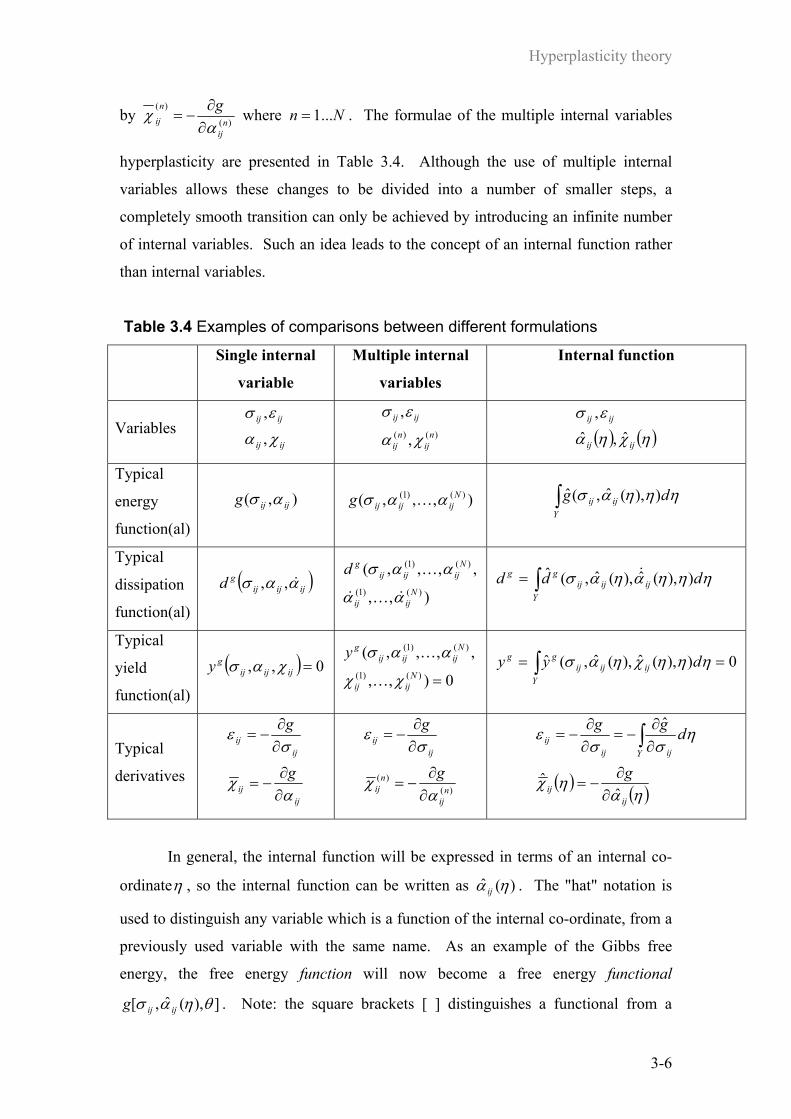
Hyperplasticity theory
3-6
by )(
)(
nij
nij
gα
χ∂∂
−= where Nn ...1= . The formulae of the multiple internal variables
hyperplasticity are presented in Table 3.4. Although the use of multiple internal
variables allows these changes to be divided into a number of smaller steps, a
completely smooth transition can only be achieved by introducing an infinite number
of internal variables. Such an idea leads to the concept of an internal function rather
than internal variables.
Table 3.4 Examples of comparisons between different formulations
Single internal
variable
Multiple internal
variables
Internal function
Variables ijij
ijij
χα
εσ
,
,
)()( ,
,n
ijn
ij
ijij
χα
εσ ( ) ( )ηχηα
εσ
ijij
ijij
ˆ,ˆ,
Typical
energy
function(al)
),( ijijg ασ ),,,( )()1( Nijijijg αασ K ηηηασ dg ijij
Y
)),(ˆ,(ˆ∫
Typical
dissipation
function(al)
( )ijijijgd αασ &,,
),,
,,,,()()1(
)()1(
Nijij
Nijijij
gd
αα
αασ
&K&
K ηηηαηασ ddd ijijijY
gg )),(ˆ),(ˆ,(ˆ &∫=
Typical
yield
function(al)
( ) 0,, =ijijijgy χασ
0),,
,,,,()()1(
)()1(
=Nijij
Nijijij
gy
χχ
αασ
K
K 0)),(ˆ),(ˆ,(ˆ == ∫ ηηηχηασ dyy ijijij
Y
gg
Typical
derivatives ij
ij
ijij
g
g
αχ
σε
∂∂
−=
∂∂
−=
)()(
nij
nij
ijij
g
g
αχ
σε
∂∂
−=
∂∂
−=
( ) ( )ηαηχ
ησσ
ε
ijij
Y ijijij
g
dgg
ˆˆ
ˆ
∂∂
−=
∂∂
−=∂∂
−= ∫
In general, the internal function will be expressed in terms of an internal co-
ordinateη , so the internal function can be written as )(ˆ ηα ij . The "hat" notation is
used to distinguish any variable which is a function of the internal co-ordinate, from a
previously used variable with the same name. As an example of the Gibbs free
energy, the free energy function will now become a free energy functional
]),(ˆ,[ θηασ ijijg . Note: the square brackets [ ] distinguishes a functional from a
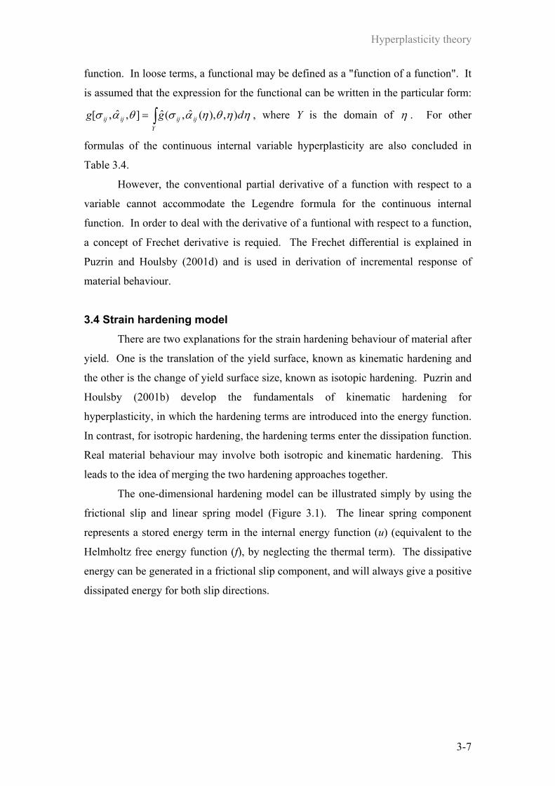
Hyperplasticity theory
3-7
function. In loose terms, a functional may be defined as a "function of a function". It
is assumed that the expression for the functional can be written in the particular form:
ηηθηασθασ dgg ijijY
ijij ),),(ˆ,(ˆ],ˆ,[ ∫= , where Y is the domain of η . For other
formulas of the continuous internal variable hyperplasticity are also concluded in
Table 3.4.
However, the conventional partial derivative of a function with respect to a
variable cannot accommodate the Legendre formula for the continuous internal
function. In order to deal with the derivative of a funtional with respect to a function,
a concept of Frechet derivative is requied. The Frechet differential is explained in
Puzrin and Houlsby (2001d) and is used in derivation of incremental response of
material behaviour.
3.4 Strain hardening model There are two explanations for the strain hardening behaviour of material after
yield. One is the translation of the yield surface, known as kinematic hardening and
the other is the change of yield surface size, known as isotopic hardening. Puzrin and
Houlsby (2001b) develop the fundamentals of kinematic hardening for
hyperplasticity, in which the hardening terms are introduced into the energy function.
In contrast, for isotropic hardening, the hardening terms enter the dissipation function.
Real material behaviour may involve both isotropic and kinematic hardening. This
leads to the idea of merging the two hardening approaches together.
The one-dimensional hardening model can be illustrated simply by using the
frictional slip and linear spring model (Figure 3.1). The linear spring component
represents a stored energy term in the internal energy function (u) (equivalent to the
Helmholtz free energy function (f), by neglecting the thermal term). The dissipative
energy can be generated in a frictional slip component, and will always give a positive
dissipated energy for both slip directions.
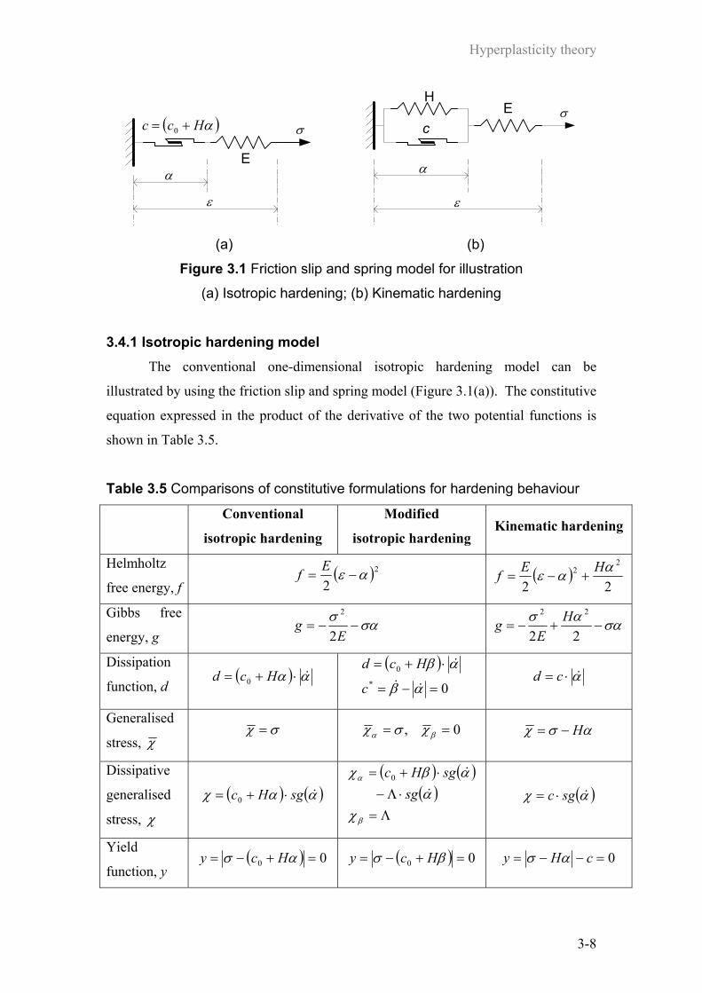
Hyperplasticity theory
3-8
ε
α E
( )αHcc += 0 σ
(a)
α
ε
cE
Hσ
(b)
Figure 3.1 Friction slip and spring model for illustration
(a) Isotropic hardening; (b) Kinematic hardening
3.4.1 Isotropic hardening model The conventional one-dimensional isotropic hardening model can be
illustrated by using the friction slip and spring model (Figure 3.1(a)). The constitutive
equation expressed in the product of the derivative of the two potential functions is
shown in Table 3.5.
Table 3.5 Comparisons of constitutive formulations for hardening behaviour
Conventional
isotropic hardening
Modified
isotropic hardening Kinematic hardening
Helmholtz
free energy, f ( )2
2αε −=
Ef ( )22
22 ααε HEf +−=
Gibbs free
energy, g σασ
−−=E
g2
2
σαασ−+−=
22
22 HE
g
Dissipation
function, d ( ) αα &⋅+= Hcd 0
( )0*
0
=−=
⋅+=
αβ
αβ
&&
&
c
Hcd α&⋅= cd
Generalised
stress, χ σχ = 0, == βα χσχ ασχ H−=
Dissipative
generalised
stress, χ
( ) ( )ααχ &sgHc ⋅+= 0 ( ) ( )
( )Λ=
⋅Λ−⋅+=
β
α
χα
αβχ&
&
sgsgHc0
( )αχ &sgc ⋅=
Yield
function, y ( ) 00 =+−= ασ Hcy ( ) 00 =+−= βσ Hcy 0=−−= cHy ασ
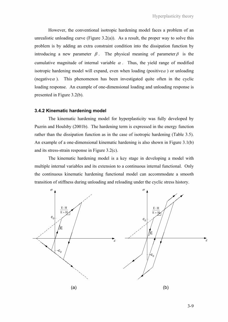
Hyperplasticity theory
3-9
However, the conventional isotropic hardening model faces a problem of an
unrealistic unloading curve (Figure 3.2(a)). As a result, the proper way to solve this
problem is by adding an extra constraint condition into the dissipation function by
introducing a new parameter β . The physical meaning of parameter β is the
cumulative magnitude of internal variable α . Thus, the yield range of modified
isotropic hardening model will expand, even when loading (positiveα ) or unloading
(negativeα ). This phenomenon has been investigated quite often in the cyclic
loading response. An example of one-dimensional loading and unloading response is
presented in Figure 3.2(b).
3.4.2 Kinematic hardening model The kinematic hardening model for hyperplasticity was fully developed by
Puzrin and Houlsby (2001b). The hardening term is expressed in the energy function
rather than the dissipation function as in the case of isotropic hardening (Table 3.5).
An example of a one-dimensional kinematic hardening is also shown in Figure 3.1(b)
and its stress-strain response in Figure 3.2(c).
The kinematic hardening model is a key stage in developing a model with
multiple internal variables and its extension to a continuous internal functional. Only
the continuous kinematic hardening functional model can accommodate a smooth
transition of stiffness during unloading and reloading under the cyclic stress history.
E
σ
c0
-c0
HEHE+⋅
ε
(a)
σ
E
ε
c0
-c0
HEHE
+⋅
(b)

Hyperplasticity theory
3-10
E
σ
ε
c
-c
2c
HEHE
+⋅
(c)
Figure 3.2 One-dimensional plot of
loading and unloading response
(a) Conventional isotropic hardening
(b) Modified isotropic hardening
(c) Kinematic hardening
3.5 Kinematic hardening function for a continuous hyperplasticity model Based on the kinematic hardening function in section 3.4.2, the bilinear stress-
strain behaviour can be described by a single internal variable. By using the multiple
internal variables, this idea can be extended to explain a piecewise linear stress-strain
behaviour. Finally, for non-linear stress-strain behaviour, a continuous internal
function is required. The comparison of the bilinear, piecewise and non-linear stress-
strain behaviours is illustrated in Figure 3.3.
σ
ε
(a)
σ
ε
(b)
σ
ε
(c)
Figure 3.3 Stress-strain relationships
(a) Bilinear; (b) Piecewise linear; (c) Non-linear
The concept of kinematic hardening hyperplasticity with a continuous internal
function can be employed to describe a continuous smooth transition from elastic to
plastic behaviour, including the case of a small finite area of the truly elastic region.
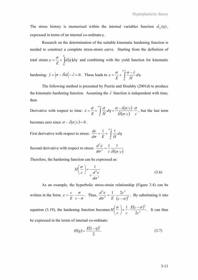
Hyperplasticity theory
3-11
The stress history is memorised within the internal variables function )(ˆ ηα ij ,
expressed in terms of an internal co-ordinateη .
Research on the determination of the suitable kinematic hardening function is
needed to construct a complete stress-strain curve. Starting from the definition of
total strain: ( )∫+=η
ηηασε0
ˆ dE
and combining with the yield function for kinematic
hardening: 0ˆˆˆˆ =−−= cHy ασ . These leads to ∫−
+=c
dHc
E
σ
ησσε0
ˆ) .
The following method is presented by Puzrin and Houlsby (2001d) to produce
the kinematic hardening function. Assuming the c function is independent with time,
then
Derivative with respect to time: ( )( ) ccH
ccdHE
c σσσσησσε
σ&
)&&
& ⋅−
++= ∫ ˆˆ
0
, but the last term
becomes zero since ( ) 0ˆ =− cc σσ .
First derivative with respect to stress: ∫+=c
dHEd
d σ
ησε
0
11)
Second derivative with respect to stress: ( )cHcd
dσσ
εˆ
112
2
=
Therefore, the hardening function can be expressed as:
2
2
1
σε
σ
ddcc
H =
(3.6)
As an example, the hyperbolic stress-strain relationship (Figure 3.4) can be
written in the form: σ
σε−
⋅=cE
c . Thus, ( )3
2
2
2 21σσ
ε−
⋅=cc
Edd . By substituting it into
equation (3.19), the hardening function becomes ( )2
3
21
ccE
ccH σσ −
⋅=
. It can thus
be expressed in the terms of internal co-ordinate:
( ) ( )2
1 3ηη −=EH (3.7)

Hyperplasticity theory
3-12
σ
ε
c
E
Figure 3.4 Hyperbolic stress-strain relationship
The continuous hyperplasticity approach allows the definition of a material
model, which gives a continuous smooth stress-strain response. However, in applying
this numerically, the continuous non-linear function has to be replaced by a piecewise
linear function. The implementation details will be given in the next section.
3.6 Hyperplasticity models for soil mechanics The hyperplasticity model for soil behaviour was first introduced by rewriting
the modified Cam Clay equation in the form of the dissipation function using a single
kinematic variable (Collins and Houlsby, 1997). Further development has continued
leading to the latest version called “kinematic hyperplasticity modified Cam-clay
model (KHMCC)” by Houlsby (2001).
In general, the development of a new material model starts from a simple
formula. Further mathematic expressions are then added to better predict stress-strain
behaviour. The model formulae and parameters should have physical meaning.
Finally, the model parameters also need tuning to correspond with experimental
results.
The following section describes the development of a new constitutive model
for soil mechanics, which begins with the one-dimensional elasticity model. The
model is then manipulated into the elasto-plastic model with a single internal variable,
multiple internal variables and a continuous internal function respectively. In
addition, the model will extend to two-dimension including triaxial stress-strain
parameters. This is useful for validation of the model with the triaxial experimental
data. The research aims to develop a soil model which will address some of the weak
σσε−
⋅=cE
c
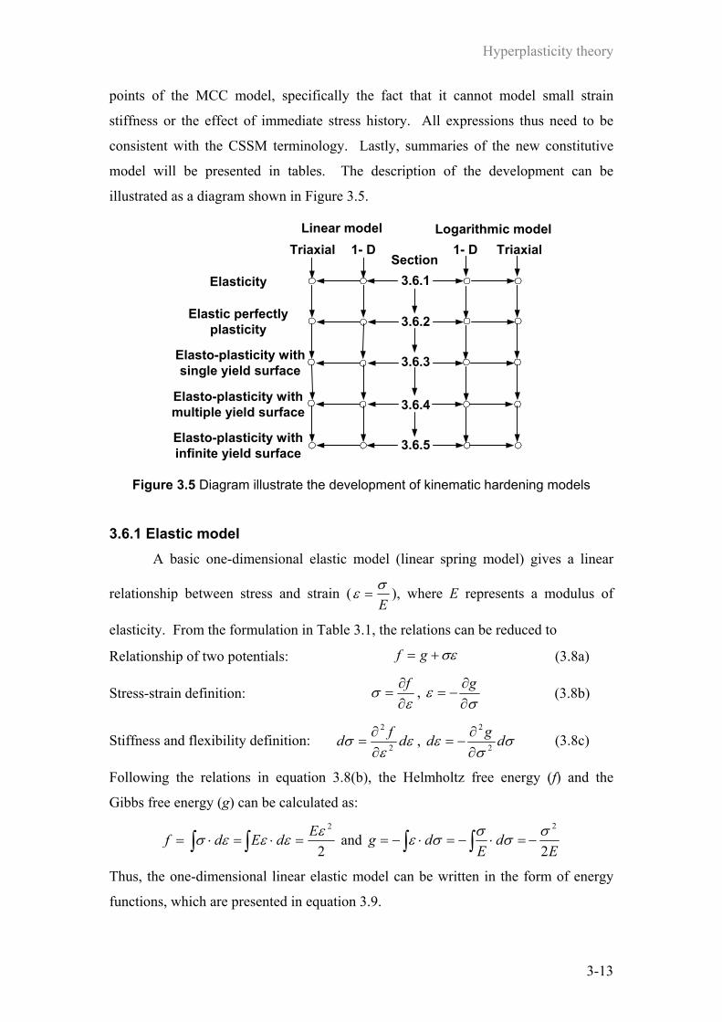
Hyperplasticity theory
3-13
points of the MCC model, specifically the fact that it cannot model small strain
stiffness or the effect of immediate stress history. All expressions thus need to be
consistent with the CSSM terminology. Lastly, summaries of the new constitutive
model will be presented in tables. The description of the development can be
illustrated as a diagram shown in Figure 3.5.
Elasticity
Linear model
Elasto-plasticity withmultiple yield surface
Elasto-plasticity withsingle yield surface
Elastic perfectlyplasticity
Elasto-plasticity withinfinite yield surface
Logarithmic model
3.6.1
3.6.5
3.6.4
3.6.3
3.6.2
1- DTriaxial 1- D TriaxialSection
Figure 3.5 Diagram illustrate the development of kinematic hardening models
3.6.1 Elastic model A basic one-dimensional elastic model (linear spring model) gives a linear
relationship between stress and strain (Eσε = ), where E represents a modulus of
elasticity. From the formulation in Table 3.1, the relations can be reduced to
Relationship of two potentials: σε+= gf (3.8a)
Stress-strain definition: ε
σ∂∂
=f ,
σε
∂∂
−=g (3.8b)
Stiffness and flexibility definition: εε
σ dfd 2
2
∂∂
= , σσ
ε dgd 2
2
∂∂
−= (3.8c)
Following the relations in equation 3.8(b), the Helmholtz free energy (f) and the
Gibbs free energy (g) can be calculated as:
2
2εεεεσ EdEdf =⋅=⋅= ∫∫ and E
dE
dg2
2σσσσε −=⋅−=⋅−= ∫∫
Thus, the one-dimensional linear elastic model can be written in the form of energy
functions, which are presented in equation 3.9.
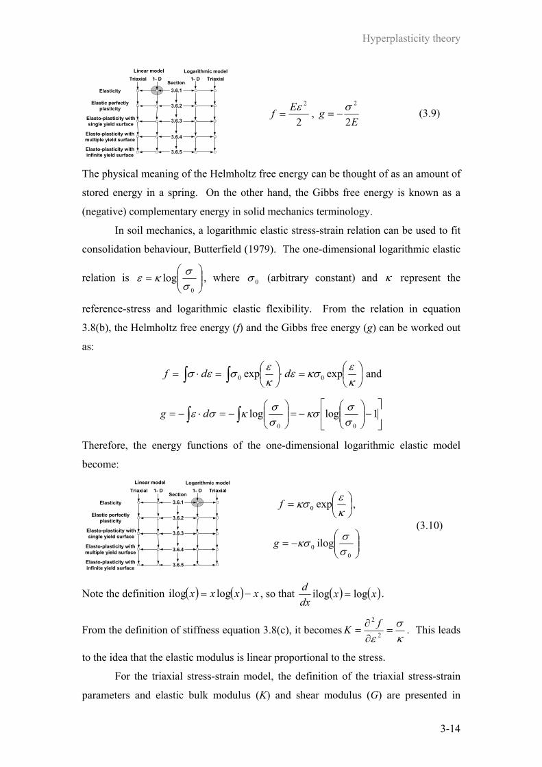
Hyperplasticity theory
3-14
Elasticity
Linear model
Elasto-plasticity withmultiple yield surface
Elasto-plasticity withsingle yield surface
Elastic perfectlyplasticity
Elasto-plasticity withinfinite yield surface
Logarithmic model
3.6.1
3.6.5
3.6.4
3.6.3
3.6.2
1- DTriaxial 1- D TriaxialSection
2
2εEf = , E
g2
2σ−= (3.9)
The physical meaning of the Helmholtz free energy can be thought of as an amount of
stored energy in a spring. On the other hand, the Gibbs free energy is known as a
(negative) complementary energy in solid mechanics terminology.
In soil mechanics, a logarithmic elastic stress-strain relation can be used to fit
consolidation behaviour, Butterfield (1979). The one-dimensional logarithmic elastic
relation is
=
0
logσσκε , where 0σ (arbitrary constant) and κ represent the
reference-stress and logarithmic elastic flexibility. From the relation in equation
3.8(b), the Helmholtz free energy (f) and the Gibbs free energy (g) can be worked out
as:
=⋅
=⋅= ∫∫ κ
εκσεκεσεσ expexp 00 ddf and
−
−=
−=⋅−= ∫∫ 1loglog
00 σσκσ
σσκσε dg
Therefore, the energy functions of the one-dimensional logarithmic elastic model
become:
Elasticity
Linear model
Elasto-plasticity withmultiple yield surface
Elasto-plasticity withsingle yield surface
Elastic perfectlyplasticity
Elasto-plasticity withinfinite yield surface
Logarithmic model
3.6.1
3.6.5
3.6.4
3.6.3
3.6.2
1- DTriaxial 1- D TriaxialSection
=κεκσ exp0f ,
−=
00 ilog
σσκσg
(3.10)
Note the definition ( ) ( ) xxxx −= logilog , so that ( ) ( )xxdxd logilog = .
From the definition of stiffness equation 3.8(c), it becomesκσ
ε=
∂∂
= 2
2 fK . This leads
to the idea that the elastic modulus is linear proportional to the stress.
For the triaxial stress-strain model, the definition of the triaxial stress-strain
parameters and elastic bulk modulus (K) and shear modulus (G) are presented in

Hyperplasticity theory
3-15
equation 2.2 and 2.3 respectively. Since, it is a fact that the elastic moduli of soils is
non-linear, i.e. the tangent moduli depend on the stress level, the bulk and shear
moduli may be written in the form of a power function of mean stress p: n
aa ppk
pK
= ,
n
ax
a ppg
pG
= (3.11)
where pa and n represent the reference mean stress and power order. This expression
can be reduced to simple linearity where n is equal to unity (i.e. pGpK ∝∝ , ). In
this research an assumption that the shear modulus (G) vary linearly with pressure
(i.e. pgG x= )1 is made.
The formulation in Table 3.1 for the triaxial stress-strain case is slightly more
complicated than for the one-dimensional case. It can be expressed in the form as
Relationship of two potentials: )( sv qpgf εε ++= (3.12a)
Triaxial stress-strain parameter definition:
sv
fqfpεε ∂∂
=∂∂
= , ; qg
pg
sv ∂∂
−=∂∂
−= εε , (3.12b)
Stiffness and flexibility matrix for triaxial stress-strain parameter:
∂∂
∂∂∂
∂∂∂
∂∂
=
s
v
ssv
svv
dd
ff
ff
dqdp
εε
εεε
εεε
2
22
2
2
2
,
∂∂
−∂∂
∂−
∂∂∂
−∂∂
−=
dqdp
qg
qpg
qpg
pg
dd
s
v
2
22
2
2
2
εε
(3.12c)
The linear elastic modulus is displayed in equation 2.3 which are vKddp ε= and
sx pdgdq ε3= . Thus, following the relation in equation 3.12(b), the Gibbs free
energy (g) can be worked out as
( ) ( )qgK
pqgdpg v 1
2
1 2+−=+⋅−= ∫ε , and ( ) ( )pg
pgqpgdqg
xs 2
2
2 6+−=+⋅−= ∫ε
Assuming there is no coupling term between p and q, g can then be expressed in
equation 3.13.
For the Helmholtz free energy (f), the assumption that p depends on not only
vε but also sε is made, and can be written in the form:
+=
23 2
sxv
gKp
εε . The
1 The subscript x is introduced to distinguish gx from g of the Gibbs free energy

Hyperplasticity theory
3-16
23 2
sxg ε term is added in order to generate the complete mathematic relation between g
and f as in equation 3.12, which introduces a small change from the original
definition. Following the same procedure for defining g, f can also be evaluated and
presented as in equation 3.13.
Elasticity
Linear model
Elasto-plasticity withmultiple yield surface
Elasto-plasticity withsingle yield surface
Elastic perfectlyplasticity
Elasto-plasticity withinfinite yield surface
Logarithmic model
3.6.1
3.6.5
3.6.4
3.6.3
3.6.2
1- DTriaxial 1- D TriaxialSection 22
23
2
+= sx
vgKf ε
ε ,
pgq
Kpg
x62
22
−−=
(3.13)
For example, from equation 3.12(c) the linear elastic stiffness matrix can be
expressed as:
−
−+=
∂∂
−∂∂
∂−
∂∂∂
−∂∂
−=
pgpgq
pgq
pgq
K
qg
qpg
qpg
pg
xx
xxe
31
3
331
2
23
2
2
22
2
2
2
K
Comparing this matrix with the elastic stiffness matrix for anisotropic soil in equation
2.4 (Graham and Houlsby, 1983), the cross-coupling term
− 23 pg
q
x
comes from
the second differentiation. This term also represents “stress-induced anisotropy”.
For the triaxial stress-strain parameters, the energy function can be calculated
based on the logarithmic elasticity in volumetric behaviour, which is dpp
d vκε = .
Conversely, the deviatoric term is still linear elasticity: pg
dqdx
s 3=ε . Thus, following
the equation 3.12(b), the Gibbs free energy (g) is calculated:
( ) ( )qgpppqgdpg v 1
001 ilog +
⋅−=+−= ∫ κε , and
( ) ( )pgpg
qpgdqgx
s 2
2
2 6+−=+−= ∫ε
and the final g expression is shown in equation 3.14. Similar to the linear case, p
should be modified and written in the form:
+=
κεε 23
exp2
0sxv g
pp . The term

Hyperplasticity theory
3-17
23 2sxg ε is added in order to generate the complete mathematic solution of equation
3.12, which introduces an insignificant modification from the original definition. The
Helmholtz free energy (f) can be evaluated in the same way as procedure for defining
g and it is presented in equation 3.14.
Elasticity
Linear model
Elasto-plasticity withmultiple yield surface
Elasto-plasticity withsingle yield surface
Elastic perfectlyplasticity
Elasto-plasticity withinfinite yield surface
Logarithmic model
3.6.1
3.6.5
3.6.4
3.6.3
3.6.2
1- DTriaxial 1- D TriaxialSection
+=
κεε
κ23
exp2
0sxv gpf ,
pgq
pppg
x6ilog
2
00 −
⋅−= κ
(3.14)
For example, from equation 3.12(c) the logarithmic elastic stiffness matrix can
be expressed as:
−
−+=
∂∂
−∂∂
∂−
∂∂∂
−∂∂
−=
pgpgq
pgq
pgq
p
qg
qpg
qpg
pg
xx
xx
31
3
33
2
23
2
2
22
2
2
2 κeK
where the cross-coupling term
− 23 pg
q
x
comes from the second differentiation and
introduces the stress-induced anisotropy to the material.
3.6.2 Elasto-plastic model with single internal variable The linear elasto-plastic model has been mentioned in section 3.5; while, the
logarithmic elasto-plasticity model will be stated in this section. A single internal
variable model offers a sudden change of modulus at yield. It behaves as purely
elastic under the yield surface and plastic once yield is reached. The stress-strain
curve is composed of two straight lines (i.e. linear elastic and perfect plastic), and it is
sometimes called the bi-linear model.
A perfectly plastic model is a special case of the elasto-plastic model, in which
there is an absence of hardening or softening. The stress-strain relations are
ασε +=E
and ασσκε +
=
0
log for linear and logarithmic elasticity respectively,
which α refers to the plastic strain. Following the stress-strain relation in equation
3.8(b), the calculation of energy functions can be processed as:
Linear model:

Hyperplasticity theory
3-18
( ) ( )2
2αεεαε −=⋅−= ∫
EdEf and
σασσασ−−=⋅
+−= ∫ E
dE
g2
2
Logarithmic model:
−
=⋅
−
= ∫ καεκσε
καεσ expexp 00 df and
σασσκσσα
σσκ −
−=⋅
+
−= ∫
00
0
iloglog dg
The energy functions of the linear and logarithmic perfect plastic model are in
equations 3.15 and 3.16 respectively.
Elasticity
Linear model
Elasto-plasticity withmultiple yield surface
Elasto-plasticity withsingle yield surface
Elastic perfectlyplasticity
Elasto-plasticity withinfinite yield surface
Logarithmic model
3.6.1
3.6.5
3.6.4
3.6.3
3.6.2
1- DTriaxial 1- D TriaxialSection ( )
2
2αε −=
Ef ,
σασ−−=
Eg
2
2
(3.15)
Elasticity
Linear model
Elasto-plasticity withmultiple yield surface
Elasto-plasticity withsingle yield surface
Elastic perfectlyplasticity
Elasto-plasticity withinfinite yield surface
Logarithmic model
3.6.1
3.6.5
3.6.4
3.6.3
3.6.2
1- DTriaxial 1- D TriaxialSection
−
=καεκσ exp0f ,
σασσκσ −
−=
00 ilogg
(3.16)
The plasticity can be modelled by using the friction slip component which
generates the dissipative energy in form the α&cd = , where c is a friction stress in the
slip component. The yield function can be calculated using Legendre transformation
( ( )αα
χ &&
sgcd⋅=
∂∂
= ), thus the dissipation and yield function are written in the form as
in equation 3.17.
Elasticity
Linear model
Elasto-plasticity withmultiple yield surface
Elasto-plasticity withsingle yield surface
Elastic perfectlyplasticity
Elasto-plasticity withinfinite yield surface
Logarithmic model
3.6.1
3.6.5
3.6.4
3.6.3
3.6.2
1- DTriaxial 1- D TriaxialSection
α&cd = , 0=−= cy χ (3.17)

Hyperplasticity theory
3-19
Note that the generalised stress is defined by α
χ∂∂
−=e , where e represents one of the
four choices of the energy function. Thus, the yield surface in the case of one-
dimensional elastic perfectly plastic becomes 0=−= cy σ , and can be drawn as in
Figure 3.6(a). If the hardening term is addressed by replacing the slip friction
component (c) with the linear hardening term ( αH ), the yield function
becomes 0=−= ασ Hy . For this case the yield surface can be plotted as in Figure
3.6(b). If the hardening term is also added into the energy function, the yield surface
might be illustrated as in Figure 3.6(c). This could be a benefit for developing a
model to describe the consolidation behaviour. To deal with this, the model with a
kinematic hardening function is considered in the next section.
σc
c-c
(a)
Hασ
Hα-Hα
(b)
Hασ
2Hα
(c)
Figure 3.6 One-dimensional yield surfaces;
(a) Elasto-plasticity, (b) Elasto-plasticity with linear hardening term,
(c) Elasto-plasticity with hardening function in the energy potential
For triaxial stress-strain parameters, the energy function has been referred to in
equation 3.13 and 3.14, but the plasticity terms ( qp αα , ) have been not yet
considered. Following the formulas in equation 3.12(b), the energy potential can be
expressed as equation 3.18 for the linear model and equation 3.19 for the logarithmic
model.
Elasticity
Linear model
Elasto-plasticity withmultiple yield surface
Elasto-plasticity withsingle yield surface
Elastic perfectlyplasticity
Elasto-plasticity withinfinite yield surface
Logarithmic model
3.6.1
3.6.5
3.6.4
3.6.3
3.6.2
1- DTriaxial 1- D TriaxialSection
( ) ( ) 2
23
2
−+−= qsx
pv
gKfαε
αε ,
( )qpx
qppg
qK
pg αα +−−−=62
22
(3.18)

Hyperplasticity theory
3-20
Elasticity
Linear model
Elasto-plasticity withmultiple yield surface
Elasto-plasticity withsingle yield surface
Elastic perfectlyplasticity
Elasto-plasticity withinfinite yield surface
Logarithmic model
3.6.1
3.6.5
3.6.4
3.6.3
3.6.2
1- DTriaxial 1- D TriaxialSection ( ) ( )
−+−=
καεαε
κ23
exp2
0qsxpv g
pf ,
( )qpx
qppg
qpppg αακ +−−
⋅−=
6ilog
2
00
(3.19)
The dissipation potential has to be chosen in order to correspond with the
elliptical yield surface of the MCC model 022
22 =−+= c
My q
p
χχ , where c is half of
the major axis of the elliptical yield surface. The reader should be reminded that the
definition of the generalised stress ( χ ), the two generalised stresses are defined
as:q
qp
peeα
χα
χ∂∂
−=∂∂
−= , , where e represents one of the four choices of the energy
function.
Firstly, assuming the dissipation is proportional to the rate of internal
variables, which is in the form of 222qp Md αα && +∝ . Next, by using the Legendre
transformation, we getp
pdα
χ&∂∂
= ,q
qdα
χ&∂∂
= . Thus, the dissipation function and the
yield function become as in equation 3.20.
Elasticity
Linear model
Elasto-plasticity withmultiple yield surface
Elasto-plasticity withsingle yield surface
Elastic perfectlyplasticity
Elasto-plasticity withinfinite yield surface
Logarithmic model
3.6.1
3.6.5
3.6.4
3.6.3
3.6.2
1- DTriaxial 1- D TriaxialSection
0222 =+⋅= qp Mcd αα && ,
0/ 222 =−+= cMy qp χχ (3.20)
Note that the shape of yield surface depends on the definition of generalised stresses
( qp χχ , ).
The shape of yield function in the case of triaxial elastic perfectly plastic
becomes 022
22 =−+= c
Mqpy , and can be drawn as in Figure 3.7(a). Similar to the
one-dimensional case, a development for the consolidation model requires an
modification of the yield function. If the slip friction component (c) is replaced by the
linear hardening term ( pHα ), the yield function becomes ( ) 022
22 =−+= pH
Mqpy α .
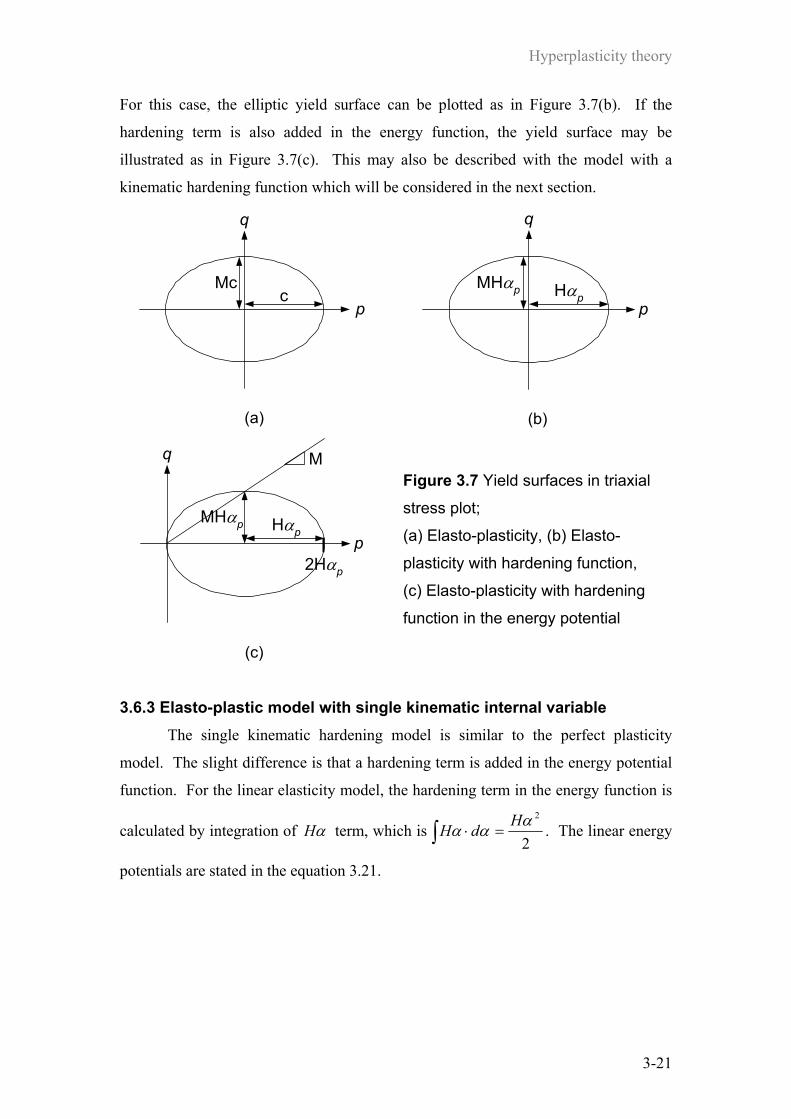
Hyperplasticity theory
3-21
For this case, the elliptic yield surface can be plotted as in Figure 3.7(b). If the
hardening term is also added in the energy function, the yield surface may be
illustrated as in Figure 3.7(c). This may also be described with the model with a
kinematic hardening function which will be considered in the next section.
p
q
cMc
(a)
MHαp Hαp
q
p
(b)
Hαp
M
2Hαp
MHαp
q
p
(c)
Figure 3.7 Yield surfaces in triaxial
stress plot;
(a) Elasto-plasticity, (b) Elasto-
plasticity with hardening function,
(c) Elasto-plasticity with hardening
function in the energy potential
3.6.3 Elasto-plastic model with single kinematic internal variable The single kinematic hardening model is similar to the perfect plasticity
model. The slight difference is that a hardening term is added in the energy potential
function. For the linear elasticity model, the hardening term in the energy function is
calculated by integration of αH term, which is ∫ =⋅2
2ααα
HdH . The linear energy
potentials are stated in the equation 3.21.

Hyperplasticity theory
3-22
Elasticity
Linear model
Elasto-plasticity withmultiple yield surface
Elasto-plasticity withsingle yield surface
Elastic perfectlyplasticity
Elasto-plasticity withinfinite yield surface
Logarithmic model
3.6.1
3.6.5
3.6.4
3.6.3
3.6.2
1- DTriaxial 1- D TriaxialSection ( )
22
22 ααε HEf +−
= ,
22
22 ασασ HE
g +−−=
(3.21)
In contrast, the logarithmic model uses an exponential hardening term, which
is calculated from ∫
=⋅
λαλσα
λασ expexp 00 d , to be included in the energy
function as in equation 3.22.
Elasticity
Linear model
Elasto-plasticity withmultiple yield surface
Elasto-plasticity withsingle yield surface
Elastic perfectlyplasticity
Elasto-plasticity withinfinite yield surface
Logarithmic model
3.6.1
3.6.5
3.6.4
3.6.3
3.6.2
1- DTriaxial 1- D TriaxialSection
+
−
=λαλσ
καεκσ expexp 00f ,
+−
−=
λαλσσα
σσκσ expilog 0
00g
(3.22)
Nevertheless, for the dissipation and yield function, the expressions used are likewise
the same as in equation 3.17.
A special feature of the consolidation behaviour of soil is that when the stress
state is touching the yield surface, the yield surface will translate and expand along
the p-axis (in triaixal stress space) as illustrated in Figure 3.6(c). This leads to the
idea of controlling the amount of the yield surface expansion to equal the amount of
the translation of yield surface’s centre, i.e. substituting αHc = or
=λασ exp0c
into equation 3.17. Thus, the yield surface becomes 0=−= αχ Hy for linear
model, and 0exp0 =
−=λασχy for logarithmic model.
The triaxial stress-strain models for the elasto-plastic model with the
kinematic internal variable are now considered. The hardening terms are required in
the equations 3.18 and 3.19 for explication of the kinematic hardening behaviour. For
the linear elastic model, the separated linear hardening terms of volumetric and shear
behaviour are used in the energy potential, which are calculated from

Hyperplasticity theory
3-23
2
2pp
ppp
HdH
ααα =⋅∫ and
2
2qq
qqq
HdH
ααα =⋅∫ respectively. The use of the
dissipation function and yield function are the same as in equation 3.20.
Elasticity
Linear model
Elasto-plasticity withmultiple yield surface
Elasto-plasticity withsingle yield surface
Elastic perfectlyplasticity
Elasto-plasticity withinfinite yield surface
Logarithmic model
3.6.1
3.6.5
3.6.4
3.6.3
3.6.2
1- DTriaxial 1- D TriaxialSection
( ) ( )
22
23
222
2
qqpp
qsxpv
HH
gKf
αα
αεαε
++
−+−=
( )
22
6222
22
qqpp
qpx
HH
qppg
qK
pg
αα
αα
++
+−−−=
(3.23)
Note that for the consolidation behaviour, the term c is replaced by ppH α as in
equation 3.20. The yield function becomes 0/ 222 =−+= ppqp HMy αχχ as
illustrated in Figure 3.7(c).
For the logarithmic relation, the hardening term ( xp ) is assumed in terms of
an exponential function. We know from the one-dimensional model that the
hardening function of pα is
⋅
λα
λ pp exp0 . The hardening function of the triaxial
model (in terms of qp αα , ) is assumed as following the elastic term in the Helmholtz
free energy (f), which is
+⋅
λεα
λ23
exp2
0sp g
p . Therefore, the final energy
potentials end up with the form as in equation 3.24.
Elasticity
Linear model
Elasto-plasticity withmultiple yield surface
Elasto-plasticity withsingle yield surface
Elastic perfectlyplasticity
Elasto-plasticity withinfinite yield surface
Logarithmic model
3.6.1
3.6.5
3.6.4
3.6.3
3.6.2
1- DTriaxial 1- D TriaxialSection
( ) ( )
+⋅+
−+−=
λεα
λ
καεαε
κ
23exp
23exp
2
0
2
0
sp
qsxpv
gp
gpf
( )
+⋅+
+−−
⋅−=
λεα
λ
αακ
23exp
6ilog
2
0
2
00
sp
qpx
gp
qppg
qpppg
(3.24)
Hyperplasticity theory
3-24
For the consolidation behaviour
+⋅==
λεα
λ23
exp2
0sp
x
gppc is replaced into
equation 3.20. This idea is employed to control the expansion of yield surface and
translation of yield surface’s centre occurring simultaneously.
In Collins and Houlsby, (1997), the MCC model was displayed in the
thermomechanics framework, in which the two potentials are defined as:
( ) ( )
−
−++−−
−
−=
κλα
κλαακ pxqp
c
pqpG
qpppg exp
61log 0
2
2220 exp qp
px Mpd αα
κλα
&& +
−
=
This model is an application of the single kinematic hardening model, in which the
shear modulus (G) is constant and the kinematic hardening term is defined following
the MCC model. The elastic and plastic bulk modulus are related to κ and λ values
as κpK = and
λpK p = respectively, where κ and λ are defined as two constant
slopes of the consolidation curve in pv ′− lnln plot. This model is one type of the
elasto-plastic model with a single kinematic hardening yield surface, in which one of
its main drawbacks is that it is purely elastic inside the yield surface and plastic on the
yield surface.
3.6.4 Elasto-plastic model with multiple kinematic internal variables Combining the idea of kinematic hardening and multiple internal variables
together, the piecewise linear stress-strain response can be built. This model can be
thought as a series of spring and friction slip components in the multiple yield
surfaces model, Iwan (1967). Following this approach, the one-dimensional linear
model with multiple kinematic internal variables can be formulated as shown in
equation 3.25 for the energy functions and equation 3.26 for the dissipation and the
yield function, Puzrin and Houlsby (2001b).
Hyperplasticity theory
3-25
Elasticity
Linear model
Elasto-plasticity withmultiple yield surface
Elasto-plasticity withsingle yield surface
Elastic perfectlyplasticity
Elasto-plasticity withinfinite yield surface
Logarithmic model
3.6.1
3.6.5
3.6.4
3.6.3
3.6.2
1- DTriaxial 1- D TriaxialSection ( ) ∑
=
+−
=n
i
iiHEf1
22
22ααε ,
∑=
+−−=n
i
iiHE
g1
22
22α
σασ
(3.25)
Elasticity
Linear model
Elasto-plasticity withmultiple yield surface
Elasto-plasticity withsingle yield surface
Elastic perfectlyplasticity
Elasto-plasticity withinfinite yield surface
Logarithmic model
3.6.1
3.6.5
3.6.4
3.6.3
3.6.2
1- DTriaxial 1- D TriaxialSection
∑=
=n
iiicd
1α& , 0=−= iii cy χ
and 01
* =−= ∑=
n
iic αα
(3.26)
Note that the total of an internal variable is the sum of each kinematic internal
variable, which plays the role of the plastic strain. This may be thought of as a
constraint condition, i.e. 01
* =−= ∑=
n
iic αα .
The dissipation function is computed from the summation of the dissipative
energy of each slip friction element, where ic is the friction stress of the ith element.
The Legendre-Fenchel transformation is used for the evaluation of the yield functions.
A simple form of the friction stress is linearly proportional to the maximum friction
stress (or size of outer yield surface). Thus, ic is generally defined as 0ccnici +
= ,
where n, 0c represent the number of the internal variable and an amount of elastic
region (for simplicity sometimes 0c is set to zero). In this research, ic is defined as
cnici
= . Furthermore, for consolidation behaviour the size of each yield surface is
simply defined as iii Hnic α
= .
For the logarithmic relation, based on equation 3.22, the energy function of the
one-dimensional logarithmic model with multiple kinematic internal variables can be
written into the equation 3.27.
Hyperplasticity theory
3-26
Elasticity
Linear model
Elasto-plasticity withmultiple yield surface
Elasto-plasticity withsingle yield surface
Elastic perfectlyplasticity
Elasto-plasticity withinfinite yield surface
Logarithmic model
3.6.1
3.6.5
3.6.4
3.6.3
3.6.2
1- DTriaxial 1- D TriaxialSection
∑=
⋅+
−
⋅=n
i i
iif
100 expexp
λα
λσκαεκσ
∑=
⋅+−
⋅−=
n
i i
iig
10
00 expilog
λα
λσσασσκσ
(3.27)
The dissipation function and the yield function of the logarithmic multiple internal
variables model also uses equation 3.26. In addition, for consolidation behaviour the
size of each yield surface is defined as
⋅
=
nic
i
ii λ
ασ exp0 .
For the triaxial stress-strain parameters, the energy functions of linear and
logarithmic multiple kinematic hardening models are evaluated and presented in
equation 3.28 and 3.29 respectively.
Elasticity
Linear model
Elasto-plasticity withmultiple yield surface
Elasto-plasticity withsingle yield surface
Elastic perfectlyplasticity
Elasto-plasticity withinfinite yield surface
Logarithmic model
3.6.1
3.6.5
3.6.4
3.6.3
3.6.2
1- DTriaxial 1- D TriaxialSection
( ) ( )
∑=
++
−+−=
n
i
iqiqipip
qsxpv
HH
gKf
1
2,,
2,,
22
23
2
αα
αεαε
( )
∑=
++
+−−−=
n
i
iqiqipip
qp
HH
qpG
qK
pg
1
2,,
2,,
22
22
62αα
αα
(3.28)
Elasticity
Linear model
Elasto-plasticity withmultiple yield surface
Elasto-plasticity withsingle yield surface
Elastic perfectlyplasticity
Elasto-plasticity withinfinite yield surface
Logarithmic model
3.6.1
3.6.5
3.6.4
3.6.3
3.6.2
1- DTriaxial 1- D TriaxialSection
( ) ( )
∑=
+⋅+
−+−=
n
i i
iqiipi
qsxpv
gp
gpf
1
2,,
0
2
0
2/3exp
23exp
λαα
λ
καεαε
κ
( )
∑=
+⋅+
+−−
⋅−=
n
i i
iqiipi
qp
gp
qpG
qpppg
1
2,,
0
2
00
2/3exp
6ilog
λαα
λ
αακ
(3.29)
For the second potentials, the dissipation function and the yield surface are
modified from equation 3.20, taking into account the multiple internal variables. The
final expressions are shown in equation 3.30.

Hyperplasticity theory
3-27
Elasticity
Linear model
Elasto-plasticity withmultiple yield surface
Elasto-plasticity withsingle yield surface
Elastic perfectlyplasticity
Elasto-plasticity withinfinite yield surface
Logarithmic model
3.6.1
3.6.5
3.6.4
3.6.3
3.6.2
1- DTriaxial 1- D TriaxialSection
01
2,
22, =+⋅= ∑
=
n
iiqipi Mcd αα && ,
0/ 22,
2, =−+= iiqipi cMy χχ
and 01
,* =−= ∑
=
n
iipppc αα ,
01
,* =−= ∑
=
n
iiqqqc αα
(3.30)
Note that the total of an internal variable is the sum of each kinematic internal
variable, which plays the role of the plastic strain. These may be thought of as two
constraint conditions, which are 01
,* =−= ∑
=
n
iipppc αα , 0
1,
* =−= ∑=
n
iiqqqc αα for pα
and qα . In addition, for consolidation behaviour in the triaxial case the size of each
yield surface can be defined as: ipipi Hnic ,, α
= and
⋅
+=
nig
pci
iqiipi λ
αα 23exp
2,,
0 for the linear and logarithmic model respectively.
3.6.5 Elasto-plastic model with continuous kinematic internal function
Following the idea of the continuous kinematic internal function )(ˆ ηα ij , a
smooth stress-strain curve can be generated. This idea is further developed from the
multiple kinematic hardening model, in which the summation of finite internal
variables is replaced by the integral of the internal function, Puzrin and Houlsby
(2001b). The energy functions of the one-dimensional models are shown in equations
3.31 and 3.32 for the linear and logarithmic models respectively.
Elasticity
Linear model
Elasto-plasticity withmultiple yield surface
Elasto-plasticity withsingle yield surface
Elastic perfectlyplasticity
Elasto-plasticity withinfinite yield surface
Logarithmic model
3.6.1
3.6.5
3.6.4
3.6.3
3.6.2
1- DTriaxial 1- D TriaxialSection ( )
∫+−
=1
0
22
2ˆˆ
2ηααε dHEf ,
∫+−−=1
0
22
2ˆˆ
2ηασασ dH
Eg
(3.31)
Hyperplasticity theory
3-28
Elasticity
Linear model
Elasto-plasticity withmultiple yield surface
Elasto-plasticity withsingle yield surface
Elastic perfectlyplasticity
Elasto-plasticity withinfinite yield surface
Logarithmic model
3.6.1
3.6.5
3.6.4
3.6.3
3.6.2
1- DTriaxial 1- D TriaxialSection ∫
⋅+
−
⋅=1
000 ˆ
ˆexpˆexp η
λασλ
καεκσ df ,
∫
⋅+−
⋅−=
1
00
00 ˆ
ˆexpˆilog η
λασλσα
σσκσ dg
(3.32)
The continuous dissipation energy and yield function are additionally shown in
equation 3.33 by Puzrin and Houlsby (2001b).
Elasticity
Linear model
Elasto-plasticity withmultiple yield surface
Elasto-plasticity withsingle yield surface
Elastic perfectlyplasticity
Elasto-plasticity withinfinite yield surface
Logarithmic model
3.6.1
3.6.5
3.6.4
3.6.3
3.6.2
1- DTriaxial 1- D TriaxialSection
∫=1
0
ˆˆ ηα dcd & , 0ˆˆˆ =−= cy χ
and 0ˆ1
0
* =−= ∫ ηαα dc
(3.33)
Note that the total of an internal variable constraint condition is 0ˆ1
0
* =−= ∫ ηαα dc .
A simple form of the c function can be defined as a linear function in the internal
coordinate. Thus, the c is generally defined as 0ˆ ccc += η , where c, 0c are arbitrary
constants. In this research, for simplicity 0c is set to zero, thus c becomes ηc .
Moreover, for consolidation behaviour of the infinite yield surface model it is simply
defined as ηαˆˆ Hc = and ηλ
α⋅
= ˆ
ˆexpˆ 0
ppc for linear and logarithmic model
respectively.
For triaxial stress-strain parameters model, the energy formulations are
expressed by equations 3.34 and 3.35 for the linear and logarithmic models
respectively.
Elasticity
Linear model
Elasto-plasticity withmultiple yield surface
Elasto-plasticity withsingle yield surface
Elastic perfectlyplasticity
Elasto-plasticity withinfinite yield surface
Logarithmic model
3.6.1
3.6.5
3.6.4
3.6.3
3.6.2
1- DTriaxial 1- D TriaxialSection
( ) ( )
∫ ++
−+
−=
1
0
22
22
2ˆˆ
2ˆˆ
23
2
ηαα
αεαε
dHH
GKf
qqpp
qspv
( )
∫ ++
+−−−=
1
0
22
22
2ˆˆ
2ˆˆ
62
ηαα
αα
dHH
qpG
qK
pg
qqpp
qp
(3.34)

Hyperplasticity theory
3-29
Elasticity
Linear model
Elasto-plasticity withmultiple yield surface
Elasto-plasticity withsingle yield surface
Elastic perfectlyplasticity
Elasto-plasticity withinfinite yield surface
Logarithmic model
3.6.1
3.6.5
3.6.4
3.6.3
3.6.2
1- DTriaxial 1- D TriaxialSection
( )
∫
+⋅+
−+
−⋅=
1
0
2
0
2
0
ˆ2/ˆˆ3ˆ
expˆ
23
exp
ηλ
ααλ
αεκαε
κ
dg
p
Gpf
qp
qspv
( )
∫
+⋅+
+−−
⋅−=
1
0
2
0
2
00
ˆ2/ˆˆ3ˆ
expˆ
6ilog
ηλ
ααλ
αακ
dg
p
qpG
qpppg
qp
qp
(3.35)
The dissipation and yield function can be modified based on the multiple yield
surfaces model in equation 3.30, and thus the formulations become as in equation
3.36.
Elasticity
Linear model
Elasto-plasticity withmultiple yield surface
Elasto-plasticity withsingle yield surface
Elastic perfectlyplasticity
Elasto-plasticity withinfinite yield surface
Logarithmic model
3.6.1
3.6.5
3.6.4
3.6.3
3.6.2
1- DTriaxial 1- D TriaxialSection
0ˆˆˆ1
0
222 =+⋅= ∫ ηαα dMcd qp&& ,
0ˆ/ˆˆˆ 222 =−+= cMy qp χχ
and 0ˆ1
0
* =−= ∫ ηαα dc ppp ,
0ˆ1
0
* =−= ∫ ηαα dc qqq
(3.36)
Note that the total internal variables are calculated from the integration of the
kinematic internal variable, which plays the role of the plastic strain. The particular
case of the c function is simply defined as a liner function with an internal
coordinate, which is ηcc =ˆ . In addition, for consolidation behaviour of the triaxial
case it can be defined as: ηα ppHc ˆˆˆ = and ηλ
αα⋅
+= ˆ
2ˆˆ3ˆexpˆ
2
0qp g
pc for the linear
and logarithmic model respectively.
The models, however, need an expression of the kinematic hardening function
which corresponds to the observed stress-strain curve. This process involves much
trial and error in order to define the mathematic formulae. Some selected hardening
functions, which are suitable for soil behaviour, will be presented in the next section.

Hyperplasticity theory
3-30
3.7 Continuous hardening function In the previous section, the continuous hardening functions are required to
define the stress-strain response for the continuous hyperplasticity model. The
continuous function provides a smooth transition of the stiffness from elastic stiffness
(when 0=η ) to plastic stiffness (when 1=η ). In order to construct the stress-strain
curve, some components of the curve must be decided upon such as the initial slope,
the asymptotic slope, and the secant or tangential slope at particular stress. This is
because a particular hardening function is able to define only one particular stress-
strain curve, for example the kinematic hardening function in equation 3.7 is used to
generate the curve in Figure 3.4. The research is conducted separately for linear and
logarithmic stress-strain relations.
3.7.1 Linear volumetric stress-strain relation Puzrin and Houlsby (2001d) showed how to define a new hardening function
based on a particular curve (backbone curve). An example of a specific form of the
hyperbolic curve is also given in that paper. A more general hyperbolic curve, which
can control the asymptote (c) and the rate of change of slope by adjusting two
additional parameters (a, b), is shown in Figure 3.8(a). A hardening function for the
general hyperbolic curve is in the form:
( )( )121ˆ−−⋅
=a
EHbη (3.37)
1
0.5
σ/c
ε/c
E
f(a)
(a)
1
0.5
σ/c
ε/c
E
f(a)
f(r)
(b) Figure 3.8 Hyperbolic stress-strain backbone curve
(a) Horizontal asymptote (b) Sloping asymptote

Hyperplasticity theory
3-31
This following section shows a mathematic proof of the hyperbolic hardening
function (equation 3.37) based on work by Puzrin and Houlsby (2001a).
General hyperbolic curve (Backbone curve)
Now, consider the first loading from cˆ =χ , and ασχ ˆˆˆ H−= thus,H
cˆ
ˆˆ −=σα
For the case ηcc =ˆ and assuming the hardening function as in equation 3.37, we
obtain:
( )( )
( )( )
( )
−−−
−−−−
+=
−−−
+=−
+=
−
−
∫∫
cbc
cEbb
aE
dcE
aE
dH
cE
b
b
c
b
c
σσ
σ
ηηησσηησσε
σσ
2)2)(1(
12
112
ˆ
2
1
00
Next, following the method presented by Puzrin and Houlsby (2001d) for general
( )ηH , we obtain:
( )( ) ( )cHcccE
add
b σσσε
ˆ1
1112
2
2
=
−−
=
Thus, the loading curve can be defined by( )cHcd
dσσ
εˆ
12
2
= , which is exactly the same
as equation 3.6.
The modified version of the hyperbolic hardening function is shown in
equation 3.38.
( )( )121ˆ
−⋅−⋅
=a
rEHbη (3.38)
The modification gives a sloping asymptote (when η approaches to 1), which is
controlled by the parameter r, see Figure 3.8(b). The r-value should be between 0
(asymptote approaches vertical) and 1 (horizontal asymptote).
Consolidation loading curve Now, we consider the loading curve of the consolidation model.
From ==== ηαηχ ˆˆˆˆˆ Hpc x , and ασχ ˆˆˆ H−= thus,( )ησα−⋅
=1ˆ
ˆH
.
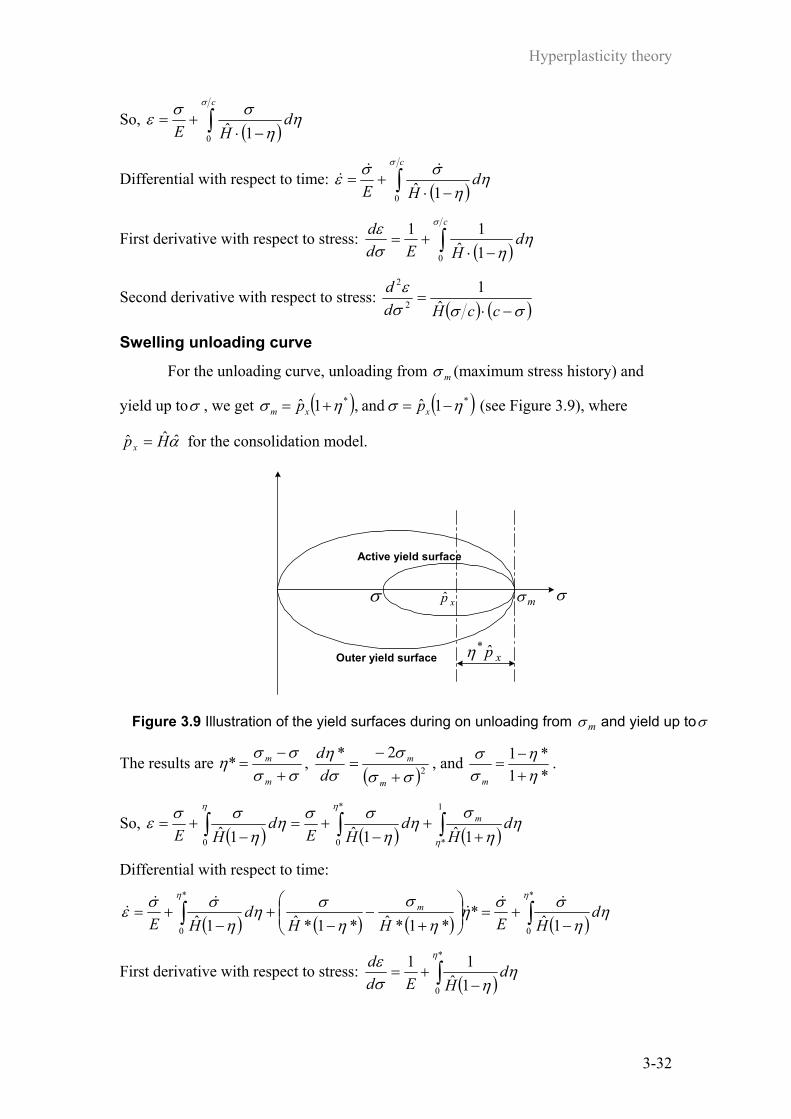
Hyperplasticity theory
3-32
So, ( )∫ −⋅
+=c
dHE
σ
ηη
σσε0 1ˆ
Differential with respect to time: ( )∫ −⋅
+=c
dHE
σ
ηη
σσε0 1ˆ
&&&
First derivative with respect to stress: ( )∫ −⋅
+=c
dHEd
d σ
ηησ
ε
0 1ˆ11
Second derivative with respect to stress: ( ) ( )σσσ
ε−⋅
=ccHd
dˆ
12
2
Swelling unloading curve
For the unloading curve, unloading from mσ (maximum stress history) and
yield up toσ , we get ( ) ( )** 1ˆand,1ˆ ησησ −=+= xxm pp (see Figure 3.9), where
αˆˆ Hpx = for the consolidation model.
xp mσσ σ
xp*ηOuter yield surface
Active yield surface
Figure 3.9 Illustration of the yield surfaces during on unloading from mσ and yield up toσ
The results are σσσσ
η+−
=m
m* , ( )2
2*σσσ
ση
+
−=
m
m
dd , and
*1*1
ηη
σσ
+−
=m
.
So, ( ) ( ) ( )∫∫∫ +
+−
+=−
+=1
*
*
00 1ˆ1ˆ1ˆη
ηη
ηη
ση
ησση
ησσε d
Hd
HEd
HEm
Differential with respect to time:
( ) ( ) ( ) ( )∫∫ −+=
+−
−+
−+=
*
0
*
0 1ˆ**1*ˆ*1*ˆ1ˆ
ηη
ηη
σσηη
ση
σηη
σσε dHEHH
dHE
m &&&
&&&
First derivative with respect to stress: ( )∫ −
+=*
0 1ˆ11 η
ηησ
ε dHEd
d

Hyperplasticity theory
3-33
Second derivative with respect to stress: ( ) ( )σσσ
σση
ησε
+
−=
−=
m
m
Hdd
Hdd
*ˆ*
*1*ˆ1
2
2
Thus, the swelling unloading curve is defined by( )σσσσ
σε
+
−=
m
m
Hdd
*ˆ2
2
.
p
εv
K Kppm
Ksec
p*
KT
(a)
lnV
λ
κκ ′
σmσm/2ln σ
(b)
Figure 3.10 Consolidation loading and unloading curve
(a) Linear stress-strain relation, (b) Logarithmic stress-strain relation
Evaluation of the hardening parameter Using the hardening function in equation 3.38, the linear consolidation
hardening function can be written as ( )( )121ˆ
−⋅−⋅
=p
b
p arKH
pη , which has four parameters
(K, ap, bp and r) in total. The following are four conditions defining the components
of the consolidation curve (see Figure 3.10(a)):
1. Initial bulk modulus K, 0→
=v
vddpK
εε
2. Tangential bulk modulus TK at particular p , ( )∫ −
+=cp
pT
dHKK 0 1ˆ
111 ηη
3. Plastic modulus PK (or asymptotic slope), ( )∫ −
+=1
0 1ˆ111 η
ηd
HKK pP
4. Secant modulus secK at particular *p ,
Hyperplasticity theory
3-34
( ) ( )∫
−−
+−+=
cp
pp
m
m
dH
pH
pppKK
*
0*
sec 1ˆ1ˆ111 η
ηη
Thus, the above four conditions are adequate to estimate the linear consolidated
parameters.
On the shearing behaviour, the shear modulus (G) is assumed to be linearly
proportional to the mean stress that is pgG x= . The shear hardening function is
assumed by equation 3.37, which is ( )
( )1213ˆ−−⋅
=q
bx
q apg
Hqη
. The additional three
parameters (gx, aq, bq) are evaluated by using the shear stress-strain curve. Firstly, the
gx value can be obtained from the initial shear modulus (shearing after the
consolidation process), which is cxini pgG = , where pc represents consolidation
pressure. The aq and bq parameters are observed using the parametric study based on
experimental results.
3.7.2 Logarithmic volumetric stress-strain relation Consolidation loading curve
Consider first loading from
==λαησχ ˆˆ
expˆˆ 0c , and
−=λασσχ ˆˆ
expˆ0
thus, ( )
+
=ησ
σλα1
logˆˆ0
( )∫
+
+
=
*
0 00 1logˆlog
η
ηησ
σλσσκε d , where η * is the largest active internal
coordinate.
Differentiating with respect to time:
( ) ∫∫ +=
+
++=*
00
*
0
ˆ**1
logˆˆηη
ησσλ
σσκη
ησσλη
σσλ
σσκε dd
&&&
&&& , since
0
*1σση =+ .
First derivative with respect to stress: ∫+=*
0
ˆη
ησλ
σκ
σε d
dd
It is noteworthy that the definition of the conventional slope of the consolidation line
is ( ) σεσ
σε
dd
dd
=log
. Thus, ( ) ∫+=*
0
ˆlog
η
ηλκσ
ε dd
d . The slope of the consolidation
line should go toλ , when η approaches to 1, and equal toκ , when 0=η .

Hyperplasticity theory
3-35
As a result, a possible function λ is assumed in the form of the power
function:
( )( ) nn ηκλλ 1ˆ +−= (3.39)
where n is the degree of power function and κ , λ are the slope of the swelling line
and normally consolidated line.
Swelling unloading curve
The form of λ is probably best determined from the unloading curve.
( ) ( )∫∫
+
+
−
+
=
1
0
*
0 00 * 1logˆ
1logˆlog
η
η
ηησ
σλη
ησσλ
σσκε dd m ,
where mσ represents the stress history.
Differential with respect to time:
( ) ( ) ( )
∫
∫
+=
⋅
+
−
−
+
−
+=
*
0
00
*
0 0
ˆ
**1
log*ˆ*1
log*ˆ1
logˆ
η
η
ησσλ
σσκε
ηησ
σλ
ησσλη
ησσλ
σσκε
d
d m
&&&
&&&
&
First derivative with respect to stress: ∫+=*
0
ˆη
ησλ
σκ
σε d
dd , so ( ) ∫+=
*
0
ˆlog
η
ηλκσ
ε dd
d .
This leads to the same equation as derived from the loading curve.
Evaluation of the hardening parameter There are three parameters (κ ,λ , and n) for the logarithmic hardening
function (equation 3.39). The κ and λ are the conventional soil parameters, which
respectively represent the slope of swelling line and normally consolidated line. The
n value can be obtained using the measure of the slope at half of the maximum past
pressure ( 2mσ ).
Let ( )σεκ
logdd
=′ at 21
=mσσ (see Figure 3.10(b)),
then from Figure 3.9, 31* =
+−
=σσσση
m
m .
Thus, 13 +=−′− n
κκκλ , in which the n value can be obtained.
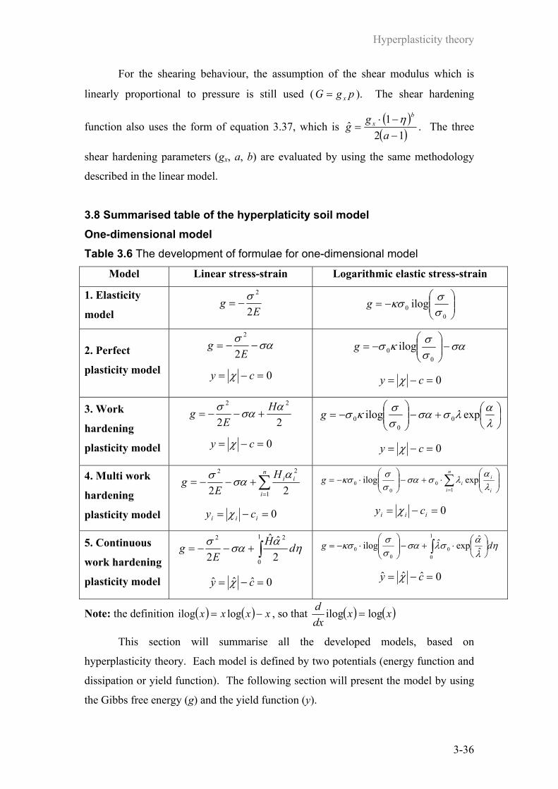
Hyperplasticity theory
3-36
For the shearing behaviour, the assumption of the shear modulus which is
linearly proportional to pressure is still used ( pgG x= ). The shear hardening
function also uses the form of equation 3.37, which is ( )( )121ˆ−−⋅
=a
gg
bx η
. The three
shear hardening parameters (gx, a, b) are evaluated by using the same methodology
described in the linear model.
3.8 Summarised table of the hyperplaticity soil model One-dimensional model Table 3.6 The development of formulae for one-dimensional model
Model Linear stress-strain Logarithmic elastic stress-strain
1. Elasticity
model Eg
2
2σ−=
−=
00 ilog
σσκσg
2. Perfect
plasticity model
σασ−−=
Eg
2
2
0=−= cy χ
σασσκσ −
−=
00 ilogg
0=−= cy χ
3. Work
hardening
plasticity model
22
22 ασασ HE
g +−−=
0=−= cy χ
+−
−=
λαλσσα
σσκσ expilog 0
00g
0=−= cy χ
4. Multi work
hardening
plasticity model
∑=
+−−=n
i
iiHE
g1
22
22α
σασ
0=−= iii cy χ
∑=
⋅+−
⋅−=
n
i i
iig
10
00 expilog
λα
λσσασσκσ
0=−= iii cy χ
5. Continuous
work hardening
plasticity model
∫+−−=1
0
22
2ˆˆ
2ηασασ dH
Eg
0ˆˆˆ =−= cy χ
∫
⋅+−
⋅−=
1
00
00 ˆ
ˆexpˆilog η
λασλσα
σσκσ dg
0ˆˆˆ =−= cy χ
Note: the definition ( ) ( ) xxxx −= logilog , so that ( ) ( )xxdxd logilog =
This section will summarise all the developed models, based on
hyperplasticity theory. Each model is defined by two potentials (energy function and
dissipation or yield function). The following section will present the model by using
the Gibbs free energy (g) and the yield function (y).

Hyperplasticity theory
3-37
The study begins with the elasticity model, followed by the perfectly plastic
model, the kinematic work hardening plasticity model, and the multi work hardening
plasticity model respectively. The development ends with the continuous work
hardening plasticity model (plus the consolidation variant for consolidation
behaviour). The above development is applied to both the linear and logarithmic type
of stress-strain behaviour as summarised in Table 3.6.
Triaxial stress-strain model Table 3.7 The development formulae of triaixal model
Model Linear volumetric
stress-strain
Logarithmic volumetric
stress-strain
1. Elasticity
model pgq
Kpg
x62
22
−−= pg
qpppg
x6ilog
2
00 −
⋅−= κ
2. Perfect
plasticity model
( )qpx
qppg
qK
pg αα +−−−=62
22
0/ 222 =−+= cMy qp χχ
( )qpx
qppg
qpppg αακ +−−
⋅−=
6ilog
2
00
0/ 222 =−+= cMy qp χχ
3. Work
hardening
plasticity model
( )
22
6222
22
qqpp
qpx
HH
qppg
qK
pg
αα
αα
++
+−−−=
0/ 222 =−+= cMy qp χχ
( )
+⋅+
+−−
⋅−=
λεα
λ
αακ
23exp
6ilog
2
0
2
00
sp
qpx
gp
qppg
qpppg
0/ 222 =−+= cMy qp χχ
4. Multi work
hardening
plasticity model
( )
∑=
++
+−−−=
n
i
iqiqipip
qpx
HH
qppg
qK
pg
1
2,,
2,,
22
22
62
αα
αα
0/ 22,
2, =−+= iiqipi cMy χχ
( )
∑=
+⋅+
+−−
⋅−=
n
i i
iqiipi
qpx
gp
qppg
qpppg
1
2,,
0
2
00
2/3exp
6ilog
λαα
λ
αακ
0/ 22,
2, =−+= iiqipi cMy χχ
5. Continuous
work hardening
plasticity model
( )
∫ ++
+−−−=
1
0
22
22
2
ˆˆ
2
ˆˆ62
ηαα
αα
dHH
qppg
qK
pg
qqpp
qpx
0ˆ/ˆˆˆ 222 =−+= cMy qp χχ
( )
∫
+⋅+
+−−
⋅−=
1
0
2
0
2
00
ˆ2/ˆˆ3ˆ
expˆ
6ilog
ηλ
ααλ
αακ
dg
p
qppg
qpppg
qp
qpx
0ˆ/ˆˆˆ 222 =−+= cMy qp χχ
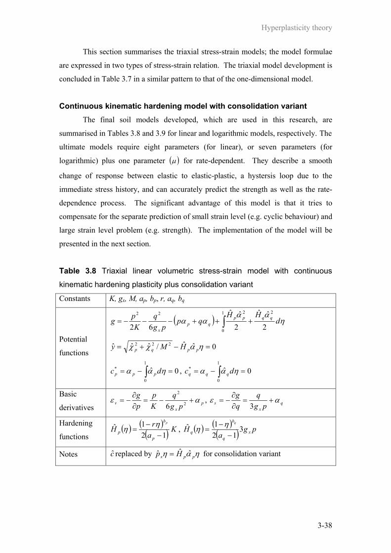
Hyperplasticity theory
3-38
This section summarises the triaxial stress-strain models; the model formulae
are expressed in two types of stress-strain relation. The triaxial model development is
concluded in Table 3.7 in a similar pattern to that of the one-dimensional model.
Continuous kinematic hardening model with consolidation variant The final soil models developed, which are used in this research, are
summarised in Tables 3.8 and 3.9 for linear and logarithmic models, respectively. The
ultimate models require eight parameters (for linear), or seven parameters (for
logarithmic) plus one parameter ( )µ for rate-dependent. They describe a smooth
change of response between elastic to elastic-plastic, a hystersis loop due to the
immediate stress history, and can accurately predict the strength as well as the rate-
dependence process. The significant advantage of this model is that it tries to
compensate for the separate prediction of small strain level (e.g. cyclic behaviour) and
large strain level problem (e.g. strength). The implementation of the model will be
presented in the next section.
Table 3.8 Triaxial linear volumetric stress-strain model with continuous
kinematic hardening plasticity plus consolidation variant
Constants K, gx, M, ap, bp, r, aq, bq
Potential
functions
( ) ∫ +++−−−=1
0
2222
2ˆˆ
2ˆˆ
62η
αααα d
HHqp
pgq
Kpg qqpp
qpx
0ˆˆ/ˆˆˆ 222 =−+= ηαχχ ppqp HMy
0ˆ1
0
* =−= ∫ ηαα dc ppp , 0ˆ1
0
* =−= ∫ ηαα dc qqq
Basic
derivatives p
xv pg
qKp
pg αε +−=∂∂
−= 2
2
6, q
xs pg
qqg αε +=∂∂
−=3
Hardening
functions ( ) ( )
( ) Ka
rHp
b
p
p
121ˆ
−−
=ηη , ( ) ( )
( ) pga
H xq
b
q
q
312
1ˆ−
−=
ηη
Notes c replaced by ηαη ppx Hp ˆˆˆ = for consolidation variant

Hyperplasticity theory
3-39
Table 3.9 Triaxial logarithmic volumetric stress-strain model with continuous
logarithmic work hardening plasticity plus consolidation variant
Constants p0 (reference pressure), κ, λ, M, gx, a, b
Definitions Note the definition ( ) ( ) xxxx −= logilog , so that ( ) ( )xxdxd logilog =
Potential
functions
( ) ∫
+++−−
−=
1
0
2
0
2
00 ˆ
2/ˆˆ3ˆexpˆ
6ilog η
λ
ααλαακ d
gpqp
pgq
pppg qp
qpx
0ˆ2/ˆˆ3ˆ
exp/ˆˆˆ2
0222 =
+−+= η
λ
ααχχ qp
qp
gpMy
0ˆ1
0
* =−= ∫ ηαα dc ppp , 0ˆ1
0
* =−= ∫ ηαα dc qqq
Basic
derivatives p
xv pg
qpp
pg ακε +−
=
∂∂
−= 2
2
0 6log , q
xs pg
qqg αε +=∂∂
−=3
Hardening
functions
( ) ( )( ) nn ηκληλ 1ˆ +−= , where ( ) 13log/log −
−′−
=κκκλn
( ) ( )( ) x
b
ga
g12
1ˆ−
−=
ηη
Notes Replaced c by ηλ
ααη
+= ˆ
2/ˆˆ3ˆexpˆ
2
0qp
x
gpp for consolidation variant
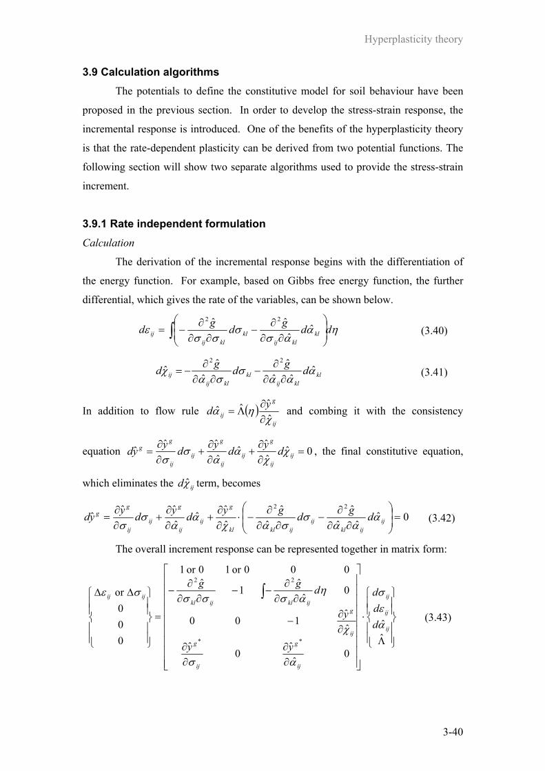
Hyperplasticity theory
3-40
3.9 Calculation algorithms The potentials to define the constitutive model for soil behaviour have been
proposed in the previous section. In order to develop the stress-strain response, the
incremental response is introduced. One of the benefits of the hyperplasticity theory
is that the rate-dependent plasticity can be derived from two potential functions. The
following section will show two separate algorithms used to provide the stress-strain
increment.
3.9.1 Rate independent formulation Calculation
The derivation of the incremental response begins with the differentiation of
the energy function. For example, based on Gibbs free energy function, the further
differential, which gives the rate of the variables, can be shown below.
ηαασ
σσσ
ε ddgdgd klklij
klklij
ij ∫
∂∂∂
−∂∂
∂−= ˆ
ˆˆˆ 22
(3.40)
klklij
klklij
ij dgdgd ααα
σσα
χ ˆˆˆ
ˆˆ
ˆˆ22
∂∂∂
−∂∂
∂−= (3.41)
In addition to flow rule ( )ij
g
ijydχ
ηαˆˆˆˆ
∂∂
Λ= and combing it with the consistency
equation 0ˆˆˆˆ
ˆˆˆˆ =
∂∂
+∂∂
+∂∂
= ijij
g
ijij
g
ijij
gg dydydyyd χ
χα
ασ
σ, the final constitutive equation,
which eliminates the ijdχ term, becomes
0ˆˆˆ
ˆˆ
ˆˆˆˆ
ˆˆˆˆ
22
=
∂∂∂
−∂∂
∂−⋅
∂∂
+∂∂
+∂∂
= ijijkl
ijijklkl
g
ijij
g
ijij
gg dgdgydydyyd α
αασ
σαχα
ασ
σ (3.42)
The overall increment response can be represented together in matrix form:
Λ
⋅
∂∂
∂∂
∂∂
−
∂∂∂
−−∂∂
∂−
=
∆∆ ∫
ˆˆ
0ˆ
ˆ0
ˆ
ˆˆ
100
0ˆ
ˆ1
ˆ000or10or1
000
or
**
22
ij
ij
ij
ij
g
ij
gij
gijklijkl
ijij
ddd
yy
y
dgg
αεσ
ασ
χ
ηασσσσε
(3.43)
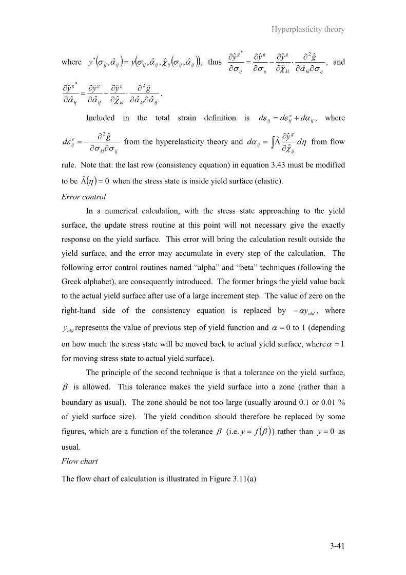
Hyperplasticity theory
3-41
where ( ) ( )( )ijijijijijijij yy ασχασασ ˆ,ˆ,ˆ,ˆ,* = , thus ijklkl
g
ij
g
ij
g gyyyσαχσσ ∂∂
∂⋅
∂∂
−∂∂
=∂∂
ˆˆ
ˆˆˆˆ 2*
, and
ijklkl
g
ij
g
ij
g gyyyααχαα ˆˆˆ
ˆˆ
ˆˆ
ˆˆ 2*
∂∂∂
⋅∂∂
−∂∂
=∂∂ .
Included in the total strain definition is ijeijij ddd αεε += , where
ijkl
eij
gdσσ
ε∂∂
∂−=
ˆ2
from the hyperelasticity theory and ∫ ∂∂
Λ= ηχ
α dydij
g
ij ˆˆˆ from flow
rule. Note that: the last row (consistency equation) in equation 3.43 must be modified
to be ( ) 0ˆ =Λ η when the stress state is inside yield surface (elastic).
Error control
In a numerical calculation, with the stress state approaching to the yield
surface, the update stress routine at this point will not necessary give the exactly
response on the yield surface. This error will bring the calculation result outside the
yield surface, and the error may accumulate in every step of the calculation. The
following error control routines named “alpha” and “beta” techniques (following the
Greek alphabet), are consequently introduced. The former brings the yield value back
to the actual yield surface after use of a large increment step. The value of zero on the
right-hand side of the consistency equation is replaced by oldyα− , where
oldy represents the value of previous step of yield function and =α 0 to 1 (depending
on how much the stress state will be moved back to actual yield surface, where 1=α
for moving stress state to actual yield surface).
The principle of the second technique is that a tolerance on the yield surface,
β is allowed. This tolerance makes the yield surface into a zone (rather than a
boundary as usual). The zone should be not too large (usually around 0.1 or 0.01 %
of yield surface size). The yield condition should therefore be replaced by some
figures, which are a function of the tolerance β (i.e. ( )βfy = ) rather than 0=y as
usual.
Flow chart
The flow chart of calculation is illustrated in Figure 3.11(a)

Hyperplasticity theory
3-42
Define two potentials: - Energy function (ex. g)- Yield function (y)
Calculate governing matrix components (ex. elastic stiffness, plastic stiffness etc.)
Set up initial condition and Specify control condition (First two lines in governing matrix)
If ( )βfy <
Apply consistency eq.
(plastic calculation)
If 0>Λ
Elastic calculation
0=Λ
Calculate yield value (y)
Update state parameters
Yes No
Yes
No
(a)
Define two potentials:
- Energy function (ex. g)
- Flow potential (w)
Set up rate-dependent constants
( µ , dt and ε& )
Solve for { }σd
Update state parameter ( )α
Update stress and strain
Set up initial condition
and Specify control statement
(S, E and T)
Calculate matrix components
(A, B, and C)
(b)
Figure 3.11 Calculation flow chart
(a) Rate-independent algorithm, (b) Rate-dependent algorithm
3.7.2 Example of rate-independent triaxial test An example of triaxial stress-strain parameters for the rate-independent
calculation algorithm is presented. Assuming that there are n numbers of yield
surfaces, the governing matrix size becomes [(2+n)nv]+1, where nv is a number of
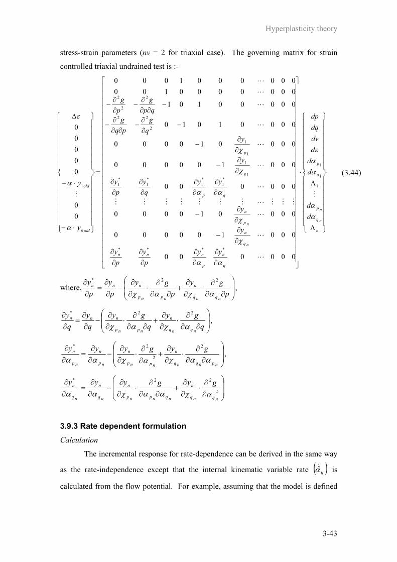
Hyperplasticity theory
3-43
stress-strain parameters (nv = 2 for triaxial case). The governing matrix for strain
controlled triaxial undrained test is :-
Λ
Λ⋅
∂∂
∂∂
∂∂
∂∂
∂∂
−
∂∂
−
∂∂
∂∂
∂∂
∂∂
∂∂
−
∂∂
−
−∂∂
−∂∂
∂−
−∂∂
∂−
∂∂
−
=
⋅−
⋅−
∆
n
nq
np
q
p
q
n
p
nnn
nq
n
np
n
qp
q
p
oldn
old
dd
ddddvdqdp
yypy
py
y
y
yyqy
py
y
yq
gpqg
qpg
pg
y
y
αα
ααε
αα
χ
χ
αα
χ
χ
α
α
ε
M
L
L
L
MMMLMMMMMMM
L
L
L
L
L
L
L
M1
1
1
****
*1
*1
*1
*1
1
1
1
1
2
22
2
2
2
1
000000
000100000
000010000
000000
000100000
000010000
00001010
00000101
00000001000000001000
00
00000
(3.44)
where,
∂∂∂
⋅∂∂
+∂∂
∂⋅
∂∂
−∂∂
=∂∂
pgy
pgy
py
py
nqnq
n
npnp
nnn
αχαχ
22*
,
∂∂∂
⋅∂∂
+∂∂
∂⋅
∂∂
−∂∂
=∂∂
qgy
qgy
qy
qy
nqnq
n
npnp
nnn
αχαχ
22*
,
∂∂∂
⋅∂∂
+∂∂
⋅∂∂
−∂∂
=∂∂
npnqnq
n
npnp
n
np
n
np
n gygyyyααχαχαα
2
2
2*
,
∂∂
⋅∂∂
+∂∂
∂⋅
∂∂
−∂∂
=∂∂
2
22*
nqnq
n
nqnpnp
n
nq
n
nq
n gygyyyαχααχαα
3.9.3 Rate dependent formulation Calculation
The incremental response for rate-dependence can be derived in the same way
as the rate-independence except that the internal kinematic variable rate ( )ijα& is
calculated from the flow potential. For example, assuming that the model is defined

Hyperplasticity theory
3-44
based on the Gibbs free energy function, the incremental relations in equation 3.40
and incorporates the derivative of flow potential ij
ijwχ
αˆ
ˆ∂∂
=& , the incremental response
can be re-expressed in the form:
dtdwgdgdklklij
klklij
ij ⋅
∂∂
⋅∂∂
∂−
∂∂∂
−= ∫ ηχασ
σσσ
εˆˆ
ˆˆ 22
(3.45)
dtwgdgdklklij
klklij
ij χαασ
σαχ
ˆˆˆˆ
ˆˆˆ
22
∂∂
⋅∂∂
∂−
∂∂∂
−= (3.46)
In addition the boundary conditions during the calculation (ex. undrained condition,
stress control etc.) are introduced by the controlling statement:
dtTdEdS ijklijklklijkl ⋅=⋅+⋅ εσ (3.47)
where S and E are stress and strain control matrices, and T is the strain or stress rate
vector.
Substituting ijdε into equation (3.47), the equation becomes:
dtdwgETdgESklklmn
ijmnijklklmn
ijmnijkl ⋅
∂∂
⋅∂∂
∂−−=⋅
∂∂
∂−+ ∫ η
χασσ
σσ ˆˆˆˆ 22
(3.48a)
or, in the matrix form: ( ) ( ){ } dtd ⋅⋅⋅⋅−=⋅⋅+ ∫ ηCBETdσAES (3.48b)
where klij
gσσ ∂∂
∂−=
ˆ2
A , klij
gασ ˆˆ2
∂∂∂
−=B , and ij
wχ∂∂
=C .
Error control
The accuracy of the rate-dependent calculation algorithm mainly depends on the time
step and the viscosity coefficient ( )µ . The artificial rate-independent process can be
approached by assuming a small value of viscosity. This would lead to a numerical
problem in the calculation of ijα& , because of the factor µ1 in the ijα& term. A
reasonable time step and strain rate must be tuned to correspond to the viscosity
value, otherwise errors from rate process would dominate.
Flow chart
The flow chart of rate-dependent algorithm is illustrated in Figure 3.11(b).

Hyperplasticity theory
3-45
3.9.4 Example of rate-dependent triaxial test An example of triaxial stress-strain parameters for the rate-dependent calculation
algorithm will also be presented. Assume that there are n numbers of yield surface;
the governing matrix for strain controlled triaxial undrained test as follows:
dtw
w
qg
qg
pg
pg
n
dqdp
qg
pqg
qpg
pg
n
i
iq
ip
iqip
iqip ⋅
∂∂∂∂
⋅
∂∂∂
−∂∂∂
−
∂∂∂
−∂∂∂
−
⋅
−
=
⋅
∂∂
−∂∂
∂−
∂∂∂
−∂∂
−⋅
+
∑=1
22
22
2
22
2
2
2
10110
0
0110
0000
χ
χ
αα
ααε&
(3.49)
3.9.5 Comparison between two approaches The most obvious benefit of the rate-dependent calculation is the including
rate dependency for materials which can exhibit any significant rate effects. Another
advantage of the rate-dependent procedure is that it is not necessary to stick with the
consistency condition (during the plasticity condition, the state always stays on the
yield surface). Thus, the higher complexity of numerical calculation is not required
for the rate-dependence. This may not require some error controlling by special
procedures that the rate-independent does. From the mathematic viewpoint, the
algorithm for rate-independence has to deal with the large size of the governing
matrix; on the other hand, the rate-dependent algorithm operates on smaller sized
matrices. As a result, it is logically shown that the computing time is reduced.
Review of experimental work
4-1
Chapter 4 Review of experimental work
In order to develop a constitutive soil model, relevant experimental soil data
are required. Two separate sets of experimental data for Bangkok clay have been
obtained from the Asian Institute of Technology (AIT), and Chulalongkorn University
in Bangkok, Thailand. The data set from AIT was gathered for the purpose of
studying the stress-strain behaviour of Bangkok clay inside the State Boundary
Surface (SBS). The experimental data set from Chulalongkorn University is focused
on the cyclic behaviour of Bangkok Clay, which is mostly concentrated on exploring
the undrained cyclic shear strength. The main purpose of this chapter is to present
and reproduce some key results from the experimental work on Bangkok clay. The
test data has been locally published as Masters theses at AIT and Chulalongkorn
University, the original copies of which are difficult for the reader to access.
Therefore, this chapter summarises the experimental techniques and conditions from
which the data is obtained. This chapter starts with a description of Bangkok clay
properties followed by the experimental programs, testing conditions and finally an
illustration of the experimental results. The advantages and disadvantages of these
experimental data are also discussed.
4.1 Geology Condition The Central Plain of Thailand consists of a flat, marine delta deposit about
300km measured north to south and about 200km east to west. These sediments
comprise alternate layers of stiff clay and dense sand aquifers down to 500m depth.
Generally, the topmost layer contains 2m thick weathered clay underlain by about 9m
of very soft clay, and followed by about 4m of soft to medium clay. Stiff clay is
encountered starting from a depth of about 15m. The thick deposit of soft clay is the
cause of substructure problems associated with low strength and high compressibility.
As a result, research on the stress-strain-strength of Bangkok clay has been
significantly developing for some time in Thailand.
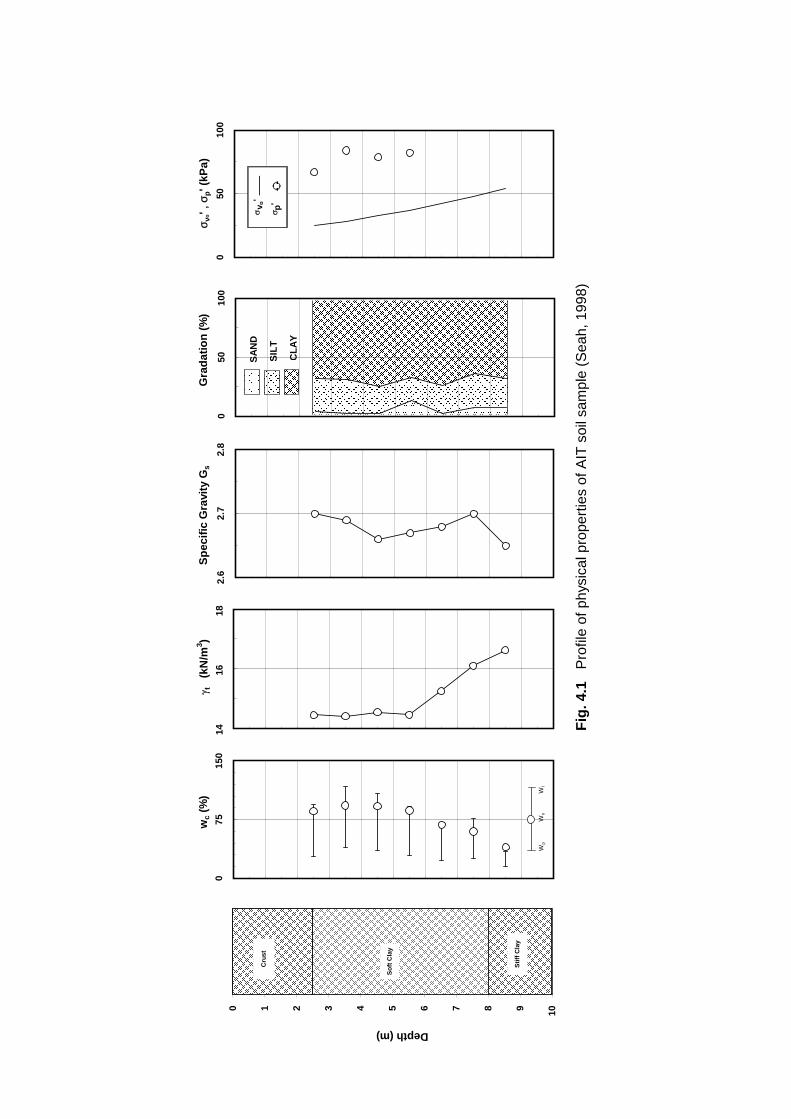
Fig
. 4.1
P
rofil
e of
phy
sica
l pro
pert
ies
of A
IT s
oil s
ampl
e (S
eah,
199
8)
075
150
1416
182.
62.
72.
80
5010
00 1 2 3 4 5 6 7 8 9 10
Cru
st
So
ft C
lay
Sti
ff C
lay
SA
ND
SIL
T
CL
AY
σ vo' ,
σp' (
kPa)
γt
(kN
/m3 )
wc
(%)
Gra
dat
ion
(%
)S
pec
ific
Gra
vity
Gs
Wp
W
n
Wl
Depth (m)
050
100
σ p'
σv o
'
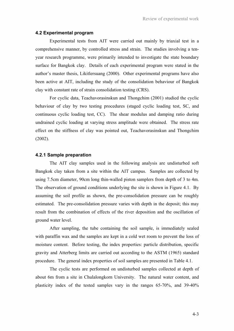
Review of experimental work
4-3
4.2 Experimental program Experimental tests from AIT were carried out mainly by triaxial test in a
comprehensive manner, by controlled stress and strain. The studies involving a ten-
year research programme, were primarily intended to investigate the state boundary
surface for Bangkok clay. Details of each experimental program were stated in the
author’s master thesis, Likitlersuang (2000). Other experimental programs have also
been active at AIT, including the study of the consolidation behaviour of Bangkok
clay with constant rate of strain consolidation testing (CRS).
For cyclic data, Teachavorasinskun and Thongchim (2001) studied the cyclic
behaviour of clay by two testing procedures (staged cyclic loading test, SC, and
continuous cyclic loading test, CC). The shear modulus and damping ratio during
undrained cyclic loading at varying stress amplitude were obtained. The stress rate
effect on the stiffness of clay was pointed out, Teachavorasinskun and Thongchim
(2002).
4.2.1 Sample preparation The AIT clay samples used in the following analysis are undisturbed soft
Bangkok clay taken from a site within the AIT campus. Samples are collected by
using 7.5cm diameter, 90cm long thin-walled piston samplers from depth of 3 to 4m.
The observation of ground conditions underlying the site is shown in Figure 4.1. By
assuming the soil profile as shown, the pre-consolidation pressure can be roughly
estimated. The pre-consolidation pressure varies with depth in the deposit; this may
result from the combination of effects of the river deposition and the oscillation of
ground water level.
After sampling, the tube containing the soil sample, is immediately sealed
with paraffin wax and the samples are kept in a cold wet room to prevent the loss of
moisture content. Before testing, the index properties: particle distribution, specific
gravity and Atterberg limits are carried out according to the ASTM (1965) standard
procedure. The general index properties of soil samples are presented in Table 4.1.
The cyclic tests are performed on undisturbed samples collected at depth of
about 6m from a site in Chulalongkorn University. The natural water content, and
plasticity index of the tested samples vary in the ranges 65-70%, and 39-40%
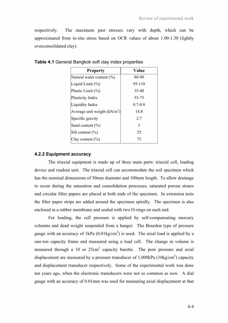
Review of experimental work
4-4
respectively. The maximum past stresses vary with depth, which can be
approximated from in-situ stress based on OCR values of about 1.00-1.30 (lightly
overconsolidated clay).
Table 4.1 General Bangkok soft clay index properties
4.2.2 Equipment accuracy The triaxial equipment is made up of three main parts: triaxial cell, loading
device and readout unit. The triaxial cell can accommodate the soil specimen which
has the nominal dimensions of 50mm diameter and 100mm length. To allow drainage
to occur during the saturation and consolidation processes, saturated porous stones
and circular filter papers are placed at both ends of the specimen. In extension tests
the filter paper strips are added around the specimen spirally. The specimen is also
enclosed in a rubber membrane and sealed with two O-rings on each end.
For loading, the cell pressure is applied by self-compensating mercury
columns and dead weight suspended from a hanger. The Bourden type of pressure
gauge with an accuracy of 1kPa (0.01kg/cm2) is used. The axial load is applied by a
one-ton capacity frame and measured using a load cell. The change in volume is
measured through a 10 or 25cm3 capacity burette. The pore pressure and axial
displacement are measured by a pressure transducer of 1,000kPa (10kg/cm2) capacity
and displacement transducer respectively. Some of the experimental work was done
ten years ago, when the electronic transducers were not so common as now. A dial
gauge with an accuracy of 0.01mm was used for measuring axial displacement at that
Property Value Natural water content (%) 80-90 Liquid Limit (%) 95-110 Plastic Limit (%) 35-40 Plasticity Index 55-75 Liquidity Index 0.7-0.8 Average unit weight (kN/m3) 14.8 Specific gravity 2.7 Sand content (%) 5 Silt content (%) 25 Clay content (%) 75

Review of experimental work
4-5
time. The accuracy achieved for load and displacement measurements varies between
the different theses cited here as different calibration procedures were used by
different authors. However, the accuracy of strain measurement of these data sets can
be estimated, based on the accuracy of the devices and dimensions of the specimen. It
is of the order of 10-4 for axial strain and 10-3 for volumetric strain.
4.2.3 Testing program
The triaxial program consists of three main processes: sample preparation,
consolidation and shearing process. The essential process of sample preparation is
to ensure that entire specimen is fully saturated, because of the simplicity of pore
pressure measurement and analysis. The specimen is saturated by balancing cell
pressure and back pressure, and then leaving the specimen for at least 24 hours before
testing.
After fully saturating the specimen, the consolidation process is implemented.
This consolidation process is done by two different approaches: isotropic
consolidation and K0-consolidation. In the first approach, the loading increment ratio1
is set to unity for the sample. The next incremental load will apply after leaving the
previous load 24 hours for ensuring fully drainage occur. The latter approach is more
complicated because cell pressure and axial stress must be applied simultaneously in
order to maintain the absence of lateral strain for K0-consolidation or other anisotropic
consolidation condition. The reduction of pressure is required for preparation of
overconsolidated samples. The overconsolidated ratio (OCR) is defined as the ratio
between the maximum past mean effective normal stress (pmax) and the current mean
effective normal stress (p).
The shearing process begins after 24 hours of consolidation or swelling to
ensure full dissipation of excess pore pressure. For stress controlled tests (only the
CID-0, CID-180, CK0D-0, CK0D-180, CAD-0 and CAD-180 tests), a mean normal
stress increment of 10kPa is used and the sample is left for 24 hours to allow the
drainage to occur. For strain controlled tests (all directions of the CID, CK0D and
CAD tests except 0o and 180o directions), the displacement rate applied for drained
tests was 0.0024mm/min and the cell pressure was continuously adjusted to maintain
1 Loading increment ratio is defined as the next load increment divided by the current applied load

Review of experimental work
4-6
the stress direction. Undrained tests (CIU tests) were conducted with constant cell
pressure and involved increasing the axial load for compression and increasing the
cell pressure for extension during undrained shearing. The sample was sheared at a
displacement rate of 0.009mm/min.
For cyclic undrained tests, the samples are firstly saturated and then
consolidated to the prescribed initial isotropic consolidation pressures: 50kPa and
100kPa. The samples tested were in a lightly overconsolidated state. The shearing
under undrained conditions was performed as stress controlled with varying rate of
loading. The shear stress amplitudes are varied from small, and moderate to large
stress levels: 0.3, 0.5 and 0.8 times unconsolidated undrained shear strength, qu
(measured from UU-test, where uu sq 2= ). In order to keep the load frequencies
constant at 0.1Hz and 1Hz, the rates of loading applied have to be automatically
adjusted corresponding with amplitude level. The testing schemes are summarised in
Table 4.2.
Table 4.2 Test scheme for cyclic undrained tests Initial consolidation
stress, (pini) Load frequency
(Hz) Stress amplitude,
(q/pini)
50
0.1, 1.0
0.1, 1.0
0.1, 1.0
0.24, 0.40
0.40, 0.60
0.60, 0.83
100
0.1, 1.0
0.1, 1.0
0.1, 1.0
0.32, 0.34
0.56, 0.52
0.80, 0.74 4.3 AIT experimental data The available triaxial experimental data from AIT are briefly summarised in
Table 4.3. The triaxial experimental data can be categorised into three groups:
consolidation data, undrained shear data and drained shear data. The detail of each
group is explained and illustrated as follows.

Review of experimental work
4-7
Table 4.3 Available triaxial experimental test data from AIT Author Year Test OCR2 η 3 Direction4 Number of tests.
Kim 1991 CIU 1.00-4.25 0 - 9
CK0UC 1.00-2.75 0.49-0.09 - 7
CK0UE 1.00-2.75 0.49-0.09 - 7
Gurung 1992 CIP 1.00-16.00 0 - 10
CIU 1.00-16.00 0 - 10
Uchaipichat 1998 CIDC 2.75 0 0-180 15
Navaneethan 1999 CIDE 2.75 0 180-360 15
Khan 1999 CK0DC 1.85 0.23 0-180 8
CK0DE 1.85 0.23 180-360 8
CK0UC 1.85 0.23 - 1
CK0UE 1.85 0.23 - 1
Tuladhar 2000 CADC 1.00 -0.27 0-180 8
CADE 1.00 -0.27 180-360 8
CAUC 1.00 -0.27 - 1
CAUE 1.00 -0.27 - 1
4.4 Consolidation data
Though there are several tests on consolidation, only some data on
consolidation hysteresis behaviour can be used. The complete load-unload-reload
loops are required for capturing the behaviour due to immediate stress history. The
consolidation data are divided into four types based on testing equipment and
condition.
4.4.1 Isotropic consolidation data from triaxial test The isotropic consolidation data are achieved from the consolidation stage of
the isotropic fan tests that were done by Uchipichat (1998) and Navaneethan (1999).
These two investigations prepared every specimen as an overconsolidated sample at
constant OCR value in isotropic consolidation condition; the consolidation stress path
2The definition of OCR-value is based on mean effective stress (p) rather than the original work that use the definition based on vertical effective stress ( vσ ′ ) 3 η is initial stress ratio (p/q) before shearing the samples 4 The direction of stress paths is measured from the p-axis in a counter clockwise direction
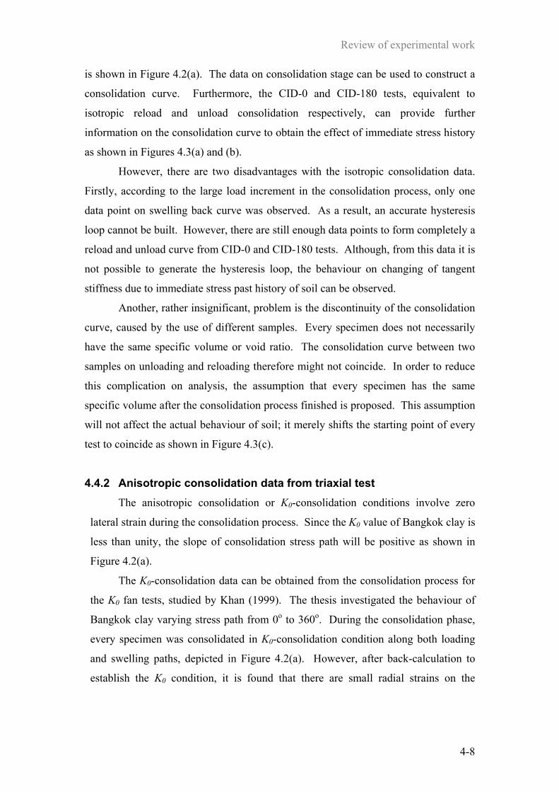
Review of experimental work
4-8
is shown in Figure 4.2(a). The data on consolidation stage can be used to construct a
consolidation curve. Furthermore, the CID-0 and CID-180 tests, equivalent to
isotropic reload and unload consolidation respectively, can provide further
information on the consolidation curve to obtain the effect of immediate stress history
as shown in Figures 4.3(a) and (b).
However, there are two disadvantages with the isotropic consolidation data.
Firstly, according to the large load increment in the consolidation process, only one
data point on swelling back curve was observed. As a result, an accurate hysteresis
loop cannot be built. However, there are still enough data points to form completely a
reload and unload curve from CID-0 and CID-180 tests. Although, from this data it is
not possible to generate the hysteresis loop, the behaviour on changing of tangent
stiffness due to immediate stress past history of soil can be observed.
Another, rather insignificant, problem is the discontinuity of the consolidation
curve, caused by the use of different samples. Every specimen does not necessarily
have the same specific volume or void ratio. The consolidation curve between two
samples on unloading and reloading therefore might not coincide. In order to reduce
this complication on analysis, the assumption that every specimen has the same
specific volume after the consolidation process finished is proposed. This assumption
will not affect the actual behaviour of soil; it merely shifts the starting point of every
test to coincide as shown in Figure 4.3(c).
4.4.2 Anisotropic consolidation data from triaxial test The anisotropic consolidation or K0-consolidation conditions involve zero
lateral strain during the consolidation process. Since the K0 value of Bangkok clay is
less than unity, the slope of consolidation stress path will be positive as shown in
Figure 4.2(a).
The K0-consolidation data can be obtained from the consolidation process for
the K0 fan tests, studied by Khan (1999). The thesis investigated the behaviour of
Bangkok clay varying stress path from 0o to 360o. During the consolidation phase,
every specimen was consolidated in K0-consolidation condition along both loading
and swelling paths, depicted in Figure 4.2(a). However, after back-calculation to
establish the K0 condition, it is found that there are small radial strains on the

Review of experimental work
4-9
swelling paths. This mean that the K0-consolidation condition occurs only on the
loading paths, whereas on the swelling paths should be treated as a stress path
control.
10 15
25
6768 126
150
180
Ko-consolidation
η = 0.23
η = -0.27
p'
consolidation pathof anisotropic fan test
q
Isotropicconsolidation
(a)
Ko - fan test
Anisotropicfan test
Isotropicfan test
p'
q
(b)
Figure 4.2 (a) Consolidation stress path, (b) Drained shear stress path (i) Isotropic fan test, Uchipichat (1998) and Navaneethan (1999), (ii) K0 fan test, Khan (1999), (iii) Anisotropic fan test, Tuladhar (2000)
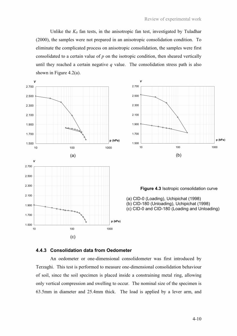
Review of experimental work
4-10
Unlike the K0 fan tests, in the anisotropic fan test, investigated by Tuladhar
(2000), the samples were not prepared in an anisotropic consolidation condition. To
eliminate the complicated process on anisotropic consolidation, the samples were first
consolidated to a certain value of p on the isotropic condition, then sheared vertically
until they reached a certain negative q value. The consolidation stress path is also
shown in Figure 4.2(a).
1.500
1.700
1.900
2.100
2.300
2.500
2.700
10 100 1000
p (kPa)
V
(a)
1.500
1.700
1.900
2.100
2.300
2.500
2.700
10 100 1000
p (kPa)
V
(b)
1.500
1.700
1.900
2.100
2.300
2.500
2.700
10 100 1000
p (kPa)
V
(c)
Figure 4.3 Isotropic consolidation curve
(a) CID-0 (Loading), Uchipichat (1998) (b) CID-180 (Unloading), Uchipichat (1998) (c) CID-0 and CID-180 (Loading and Unloading)
4.4.3 Consolidation data from Oedometer
An oedometer or one-dimensional consolidometer was first introduced by
Terzaghi. This test is performed to measure one-dimensional consolidation behaviour
of soil, since the soil specimen is placed inside a constraining metal ring, allowing
only vertical compression and swelling to occur. The nominal size of the specimen is
63.5mm in diameter and 25.4mm thick. The load is applied by a lever arm, and

Review of experimental work
4-11
compression is measured by a dial gauge with an accuracy 0.01mm. The specimen is
kept under water to maintain the saturation of the soil sample. The load increment
ratio is set to unity, and remains at this level for at least 24 hours until the next load
increment applied.
The consolidation data from oedometer can be simplified as a K0-
consolidation condition, because there is no lateral strain occuring during the
compression. Data interpretation on the logarithmic or square root of time plot are
required to evaluate the end of primary consolidation. The calculated effective stress
is based on the assumption of a parabolic pore water pressure distribution and if the
tests are slow enough there will be zero pore pressure at the end of each stage. The
analysis must be repeated at every data point to generate the complete consolidation
curve. The oedometer test data were obtained by Seah and Hassan (1999). The
oedometer tests were conducted with one loading increment per day up to a maximum
vertical pressure of 1,600kPa. The tests were performed on samples from 3.5m and
4.5m. The oedometer results at 3.5m are shown in Figure 4.4(a).
The weak point of the data comes from the limitation of the oedometer itself.
Firstly, there are fewer data points on the consolidation curve, particularly during the
swelling curve. This is because the assumption of pore pressure distribution cannot
be applied to the water absorbed during the swelling process. Thus, the data
interpretation procedure (logarithmic or square root time plot) cannot be processed on
the unloading curve correctly. The data point was therefore observed only at the end
of the testing program. Moreover, due to the inconstant strain rate during the testing
programme, the effect of viscosity is included in the consolidation result.
4.4.4 Consolidation data from CRS test In order to improve the one-dimensional consolidometer test, the constant rate
of strain (CRS) consolidometer is introduced. This is because the conventional
consolidometer usually applies the load increment ratio equal to one for the duration
of one day, giving a total testing period consisting of one to two weeks. The resulting
compression curve may be poorly defined, especially near the maximum past stress.
For example, in sensitive clay, it is frequently recommended to use a low strain rate in
order to capture the behaviour near the maximum past stress. However, a small strain
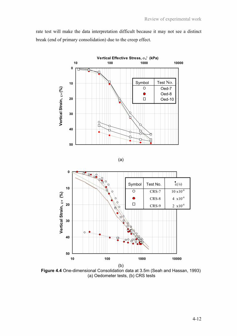
Review of experimental work
4-12
rate test will make the data interpretation difficult because it may not see a distinct
break (end of primary consolidation) due to the creep effect.
0
10
20
30
40
50
10 100 1000 10000Vertical Effective Stress, σv' (kPa)
Verti
cal S
train
, εv
(%)
(a)
0
10
20
30
40
5010 100 1000 10000
Verti
cal S
train
, εv
(%)
(b)
Figure 4.4 One-dimensional Consolidation data at 3.5m (Seah and Hassan, 1993) (a) Oedometer tests, (b) CRS tests
Symbol Test No.
Oed-8 Oed-7
Oed-10
CRS-9
Test No.Symbol
CRS-7
CRS-8
ε(/s)
10 x10-6
4 x10⁻⁶
2 x10⁻⁶

Review of experimental work
4-13
In the CRS consolidometer test, the soil sample is loaded continuously, rather
than incrementally, at the rate required to produce a desired constant rate of strain one
dimensionally with one end drainage at the top. Back pressure can be applied on the
sample to improve the degree of saturation. The pore water pressure develops at the
lower end of the sample. During the test, continuous reading of the loads
corresponding to the strain and the pore water pressure at the base are obtained.
These data allow a continuous compression curve to be produced with greater
objectivity.
The CRS consolidometer used consists of base plate from a triaxial cell,
sample-retaining ring from oedometer and loading cell at a constant speed. The
sample size is the same as the oedometer sample, and the pressure transducer is
connected at the base plate to measure the pore water pressure. In order to achieve
the single drainage condition, a coarse porous stone is attached to the top cap.
The CRS tests were carried out by Seah and Hassan (1999), and Seah and
Juirnarongrit (1999). The CRS tests were conducted with three different strain rates
between 10-5 and 2x10⁻⁶ /s. The tests were performed up to a maximum vertical
pressure of 1,600kPa on samples from 3.5 and 4.5m. The CRS results, at depth of
3.5m, are shown in Figure 4.4(b).
4.5 Undrained shear data The undrained shear data can be divided into two groups based on the
consolidation process.
The isotropic consolidation undrained shear (CIU) data come from two studies
which were done by Kim (1991) and Gurung (1992). Kim’s CIU tests were done by
varying the OCR value from 1.00 to 4.25, but each specimen was not consolidated to
the same pre-consolidation pressure. To reduce the complexity of analysis, the data
was normalised by the maximum past value of mean stress, which is equal to the
vertical pre-consolidation stress in this case. The normalised undrained stress path of
the OCR value varying from 1.00 to 4.25 is shown in Figure 4.5(a). Another source
of CIU data is obtained from Gurung (1992). The CIU tests were carried out by
varying the OCR value from 1.00 to 16.00, consolidated to the same value of
maximum past pressure.

Review of experimental work
4-14
The K0-consolidation undrained shear (CK0U) data has also been obtained
from Kim (1991). These CK0U tests were done by varying the OCR value from 1.00
to 4.25, in which each specimen was consolidated under K0-swelling conditions at the
same maximum past pressures. There are two sets of data, namely compression
(CK0UC) and extension (CK0UE) as shown in Figure 4.5(b).
0.00
0.20
0.40
0.60
0.80
1.00
1.20
0.00 0.20 0.40 0.60 0.80 1.00 1.20 1.40
p/pmax
q/pmax
(a)
-1.00
-0.80
-0.60
-0.40
-0.20
0.00
0.20
0.40
0.60
0.80
1.00
0.00 0.20 0.40 0.60 0.80 1.00 1.20 1.40p/pmax
q/pmax
(b)
Figure 4.5 Undrained shear test (Kim, 1990) (a) CIU test (b) CKU test
A possible weak point of Kim's undrained shear data is its unreliability due to
the fact that the research investigation took a total of four years. Every soil sample
was collected from the site at the same time and kept for more than two years.
Therefore, the in-situ stress and moisture content might decrease due to aging effects.
The specimen may be stiffer than its original behaviour. For Gurung’s data, the
electronic data is not supplied directly, however the secondary data were measured
from the stress-strain curve by Likitlersuang (2000). As a result, an error from human
measurement is added into these data.
4.6 Drained shear data
There are three complete sets of investigations on the triaxial drained
behaviour of overconsolidated clay. Each study program consists of two phases: the
consolidation phase and shearing phase. For the consolidation phase, each study

Review of experimental work
4-15
consolidated the specimens using different consolidation conditions, namely the
isotropic, K0, and anisotropic condition. The different consolidation stress paths are
already described in the consolidation data section as illustrated in Figure 4.2(b). For
the shearing phase, all studies sheared the specimens varying the stress path direction
from 0o to 360o as presented in Figure 4.2(b).
The isotropic fan tests (CID) were carried out by Uchaipichat (1998) and
Navaneethan (1999), (compression and extension drained shear tests respectively). A
total of 30 tests were sheared in a comprehensive manner which spread from the
centre point in a fan shape and all have the same stress history from the isotropic
overconsolidated stage. Therefore, the isotropic data can be used to validate the soil
model efficiently; by using the soil model to generate the numerical stress-strain data
in each shearing direction, a comparison with experimental data can be obtained. A
plot of volumetric and shear strain parameter )( 22sv εε + contour can be constructed
as shown in Figure 4.6.
However, the stress-strain data, which were tested under different rates of
strain conditions, can be observed from the contour plot. The CID-0 and CID-180
tests were carried out by stress controlled conditions which use the load increment
equal to 20kPa and 10kPa per step for loading and unloading respectively, and takes
24 hours allowing for the drainage. Thus, the CID-0 and CID-180 tests have taken 9
days and 6 days respectively. For other strain controlled tests, the strain increment of
0.0024mm/min have been used. The average time of strain controlled tests is roughly
3 days. The result of the using of two different rates is implied in Figure 4.6, where
the contour points of CID-0 and CID-180 tests are very close together than others.
The viscosity effects or rate effects have to be considered, as a result.
The K0 fan test (CKD) and anisotropic fan test (CAD) were carried out by
Khan (1999), and Tuladhar (2000), respectively. The CKD and CAD tests were
sheared in a comprehensive manner, which spread from the centre point in a fan
shape. However, in the consolidation process, the CKD tests were consolidated with
the K0-condition, the CAD tests on the other hand were consolidated by the isotropic
condition first and then constant-p shearing until they reach the anisotropic line as
already described in consolidation data. The CKD and CAD test data can be used to
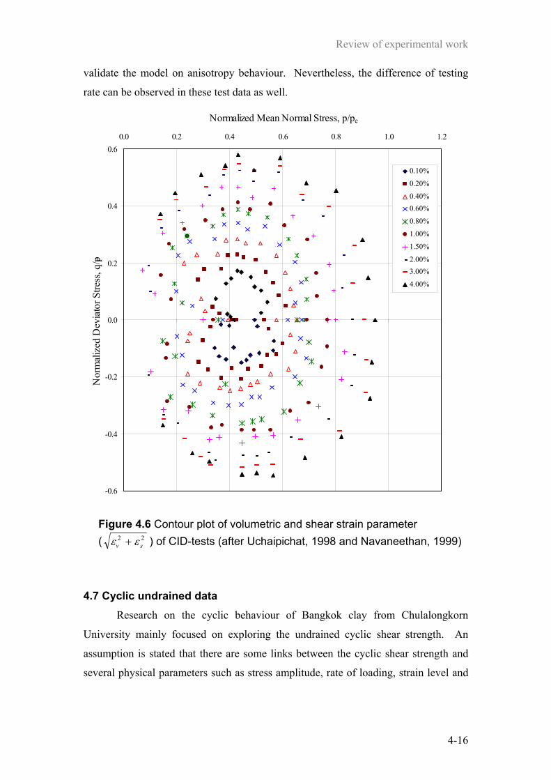
Review of experimental work
4-16
validate the model on anisotropy behaviour. Nevertheless, the difference of testing
rate can be observed in these test data as well.
-0.6
-0.4
-0.2
0.0
0.2
0.4
0.60.0 0.2 0.4 0.6 0.8 1.0 1.2
Normalized Mean Normal Stress, p/pe
Nor
mal
ized
Dev
iato
r Stre
ss, q
/p e
0.10%
0.20%
0.40%0.60%
0.80%
1.00%
1.50%
2.00%3.00%
4.00%
4.7 Cyclic undrained data Research on the cyclic behaviour of Bangkok clay from Chulalongkorn
University mainly focused on exploring the undrained cyclic shear strength. An
assumption is stated that there are some links between the cyclic shear strength and
several physical parameters such as stress amplitude, rate of loading, strain level and
Figure 4.6 Contour plot of volumetric and shear strain parameter ( 22
sv εε + ) of CID-tests (after Uchaipichat, 1998 and Navaneethan, 1999)

Review of experimental work
4-17
number of load cycles. The shear stress amplitude was defined, based on the
unconsolidated undrained (UU-Test) shear strength ( uu sq 2= ), as small, moderate,
and large amplitude levels. The cyclic tests data were carried out under initial
isotropic consolidation stress: 50kPa and 100kPa. The rate of loading was at two
constant frequencies of 0.1Hz and 1.0Hz.
The cyclic undrained shear strength behaviour can be determined by the
values of secant shear modulus (Gsec) and damping ratio (hc) as shown in Figure 4.7.
The initial shear modulus obtained at a small strain level of about 0.02-0.05% were
measured for all samples and compared with the shear wave velocity measurement at
field, which gave a reasonable agreement value about 13-15MPa. Moreover, the
semi-log plot of the shear modulus (G) with the single amplitude shear strain ( SAγ ) is
illustrated. The calculation of the damping ratio, which can represent the shape of
hystersis loop, was performed in this research. The relationship between the damping
ratio and the single amplitude shear strain is shown in Figure 4.7. Moreover, the
effect of rate of loading on cyclic properties was investigated. Because of the small
frequency difference between 0.1Hz and 1Hz, it does not show a significant effect on
shear modulus and damping ratio.
Due to the lack of the information on stress history of tested samples,
estimations of maximum stress past are required. Based on the other research on
Bangkok clay, there is some evidence showing that the top Bangkok clay soil layer is
lightly overconsolidated (approximated OCR value about 1.20). The maximum past
stress can be roughly estimated from the OCR value and in-situ stress. However, the
research pointed out that the in-situ stress of tested samples is around 90-100kPa.
These experimental data on cyclic load are particularly useful for the
validation of the model, because they consider the variation of stiffness at small strain
level. However, some significant information about testing procedure such as
sampling procedure, maximum past stress and also the parameter definitions used in
this research is not available. The confusion of stress-strain parameters has to be
eliminated by using Cambridge triaxial stress-strain parameters. The evidence on the
monotonic undrained compression test found that Chulalongkorn’s clay samples are
slightly stiffer than AIT’s samples. The natural water content and plasticity index are

Review of experimental work
4-18
also illustrated this same trend. However, this is not a significant issue for the
parametric evaluation and will be discussed in the next chapter.
0
1
2
3
4
5
6
7
8
9
10
0.0010 0.0100 0.1000 1.0000
γ(−)
G (MPa)
q/p =0.32
q/p =0.56
q/p =0.80
(a)
0
5
10
15
20
25
30
35
40
45
0.0010 0.0100 0.1000 1.0000
γ(−)
hc (%)
q/p =0.32
q/p =0.56
q/p =0.80
(b)
Figure 4.7 Cyclic Undrained Shear Test varying shear stress magnitude (q/p) at confining pressure (pc) = 100kPa (Teachavorasinskun and Thongchim, 2001)
(a) Plot of shear modulus (G) vs. single amplitude shear strain ( SAγ )
(b) Plot of damping ration (hc) vs. single amplitude shear strain ( SAγ )
Review of experimental work
4-19
4.8 Conclusion Almost all soil models focus on either large strain (near failure) or small strain
behaviour. It is rarely the case that a soil model can describe both behaviours. In
order to develop a model, the experimental data at both small strain and large strain
behaviours, which are carried out on the same material, are required.
A series of experimental investigations on stress-strain-strength behaviour of
Bangkok clay were carried out at AIT and Chulalongkorn University. There are
several categories of testing programs: consolidation test, undrained shear test and
drained shear test as well as cyclic loading test.
Consolidation data can be divided into four types, based on the testing
equipment and conditions: isotropic triaxial consolidation, anisotropic triaxial
consolidation, oedometer test and CRS consolidometer test. The triaxial
consolidation data is mainly obtained from of the consolidation phase of undrained
shear and drained shear tests. The research on one-dimensional consolidation was
investigated widely at AIT, employing an improved consolidometer called a CRS
consolidometer. Although, there are many sets of consolidation data available, only
some of them can be used to construct the hysteresis loop, which is important for the
current research.
The undrained and drained shear data can be divided into two groups based on
the consolidation process: isotropic and anisotropic consolidation. The accuracy of
the undrained shear data is subjected to the testing programme which took about four
years. This makes the sample stiffer than its original behaviour due to aging effects.
The drained shear data are obtained from the three series of the fan test. The major
disadvantage of drained shear data is the usage of different testing conditions, namely
the stress-controlled test on the horizontal direction and the strain-controlled test in
the other directions. These two different testing conditions also used two different
rates of loading, which is significant for the analysis using rate-dependent calculation.
The result is implied in the plot of strain contour as illustrated in Figure 4.6.
The experimental data at small strain levels can be achieved from the research
on cyclic undrained shear at Chulalongkorn University. This research provides the
information on the variation of shear modulus and damping ratio. However, although
the rate of loading was studied in the research, it does not point out that different rates

Review of experimental work
4-20
of loading would produce significantly different effects. Due to the lack of stress
history information, reasonable values have to be estimated. Moreover, evidence on
monotonic undrained compression test found that Chulalongkorn’s samples are
slightly stiffer than those of AIT.

Comparisons, Results and Discussion
5-1
Chapter 5 Comparisons, Results and Discussion
A hyperplasticity model in terms of triaxial stress-strain parameters has been
developed as presented in chapter 3. The experimental data for Bangkok clay have
been obtained from AIT and Chulalongkorn University. All experimental programs
have been already described in the previous chapter. In this chapter, some
comparisons between experimental data and model predictions based on a particular
set of parameters will be presented. The comparisons can be categorised into four
types based on the type of data: consolidation, undrained, drained, and cyclic
undrained data.
The predictions of the KHMCC model are compared with all experimental
data. Both linear and logarithmic stress-strain relations are used. The linear model,
however, seems to provide a better result than the logarithmic model, especially on
swelling data from consolidation tests. Another advantage of using the linear model
is the simplicity of the calculation. Nevertheless, from the CSSM viewpoint, the
definition of compression parameters ( )κλ , is defined based on v-log p plot. The log
v-log p plot introduced by Butterfield (1979) shows that it is not necessary to retain
with the v-log p plot in describing the consolidation behaviour. The compression
curve can be defined in other ways, and one possible stress-strain relation is a simple
linear one. As a result, the simple linear stress-strain relation is used to define the soil
behaviour in this research.
Tables 5.1(a) and (b) summary all parameters and their physical meaning
based on Bangkok clay experimental data for the linear model and the MCC model
respectively.
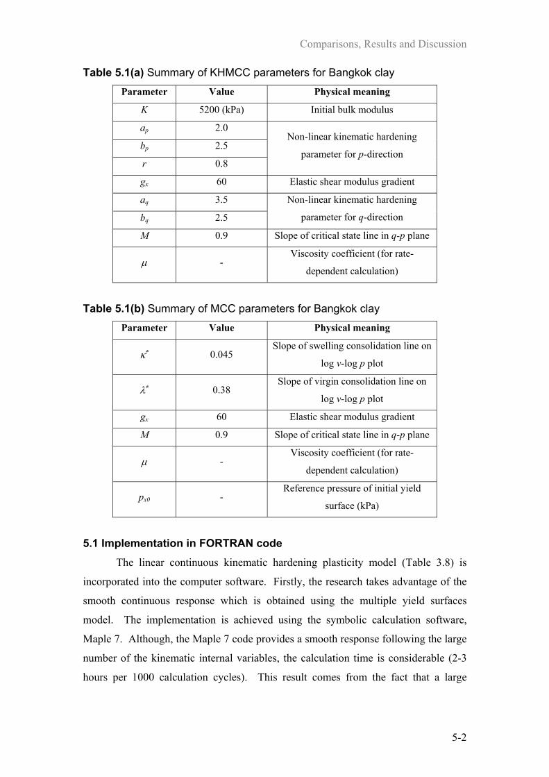
Comparisons, Results and Discussion
5-2
Table 5.1(a) Summary of KHMCC parameters for Bangkok clay
Parameter Value Physical meaning
K 5200 (kPa) Initial bulk modulus
ap 2.0
bp 2.5
r 0.8
Non-linear kinematic hardening
parameter for p-direction
gx 60 Elastic shear modulus gradient
aq 3.5
bq 2.5
Non-linear kinematic hardening
parameter for q-direction
M 0.9 Slope of critical state line in q-p plane
µ - Viscosity coefficient (for rate-
dependent calculation)
Table 5.1(b) Summary of MCC parameters for Bangkok clay
Parameter Value Physical meaning
κ∗ 0.045 Slope of swelling consolidation line on
log v-log p plot
λ∗ 0.38 Slope of virgin consolidation line on
log v-log p plot
gx 60 Elastic shear modulus gradient
M 0.9 Slope of critical state line in q-p plane
µ - Viscosity coefficient (for rate-
dependent calculation)
px0 - Reference pressure of initial yield
surface (kPa)
5.1 Implementation in FORTRAN code The linear continuous kinematic hardening plasticity model (Table 3.8) is
incorporated into the computer software. Firstly, the research takes advantage of the
smooth continuous response which is obtained using the multiple yield surfaces
model. The implementation is achieved using the symbolic calculation software,
Maple 7. Although, the Maple 7 code provides a smooth response following the large
number of the kinematic internal variables, the calculation time is considerable (2-3
hours per 1000 calculation cycles). This result comes from the fact that a large

Comparisons, Results and Discussion
5-3
amount of computer memory is needed for symbolic calculation, and an experiment
has revealed that the symbolic calculation is 100 times more time-consuming than
arithmetic calculation.
In order to make the smooth continuous plasticity model more practical, the
multiple yield surfaces model is considered. The numerical approach for the multiple
yield surfaces model is implemented in FORTRAN 90. This will give an advantage
in the next stage of the research on application into the OXFEM program, because
OXFEM was written in FORTRAN. Numerical problems such as rounding error can
be controlled by using double precision numbers (10-16 accuracy) rather than single
precision (10-8). The calculation accuracy also depends on other factors (eg. number
of yield surfaces, time step, and viscosity coefficient). The greater the number of
yield surfaces used, the smoother the response generated. Use of too many yield
surfaces, however, may lead to a computation time problem. This study uses fifty
yield surfaces for comparisons with triaxial experimental data and ten yield surfaces
for cyclic data. The effect of viscosity will be described in the next section.
5.2 Consolidation behaviour prediction The consolidation behaviour prediction is calculated from the KHMCC
model, however, the model can be reduced to the one-dimensional model as shown in
Table 3.6. The evaluation based on a rate-dependent algorithm assumes the set of
viscosity parameters to have no effect. This seems to be artificial rate-independence,
which use a small viscosity value µ . The study on the viscosity effect on the stress-
strain behaviour has found that the strength of material depends on a product of
coefficient of viscosity and strain rate ( )εµ & as shown in Figure 5.1(a). This
relationship is in terms of an exponential function, i.e. the material strength will grow
rapidly with increasing of εµ & value (see Figure 5.1(b)). However, at small values εµ & ,
the rate effect will not be significant. This leads to an approximation of the rate-
independent response.
The predicted results compare isotropic consolidation along unloading-
reloading curves in term of mean stress (p). The evaluation has found that the linear
model gives a more reasonable volumetric strain on the swelling path than the
logarithmic model. This continuous kinematic hardening model results comply
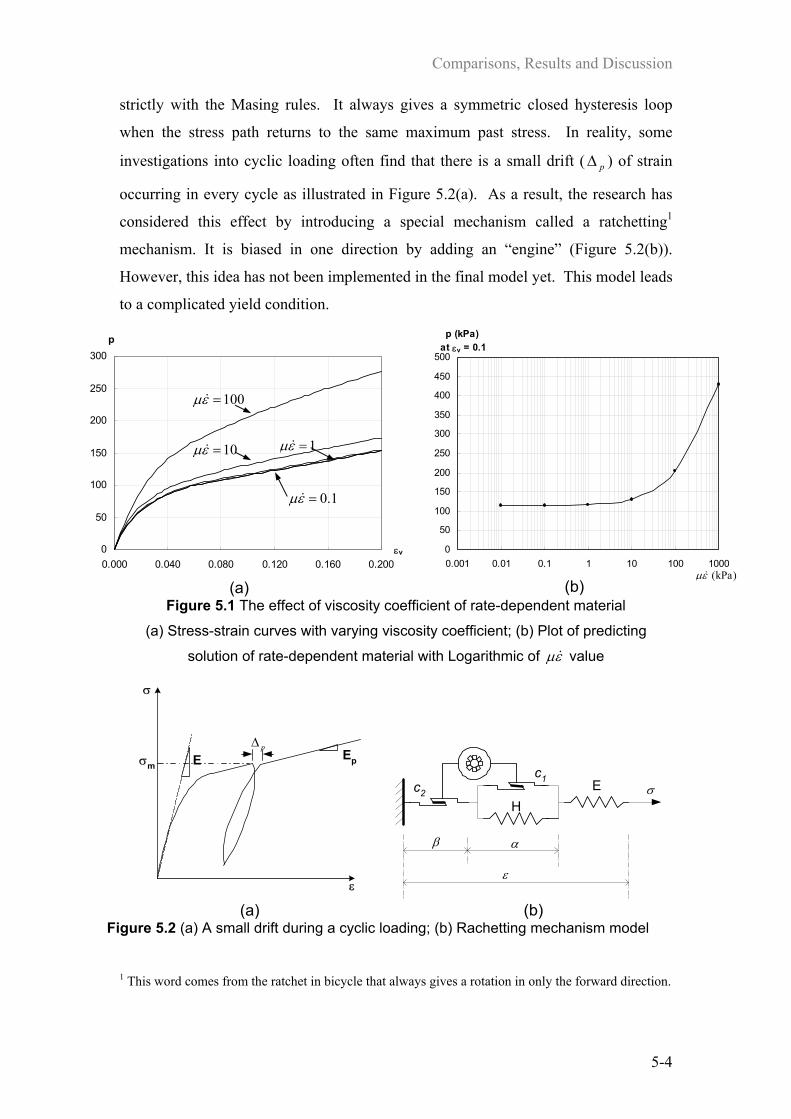
Comparisons, Results and Discussion
5-4
strictly with the Masing rules. It always gives a symmetric closed hysteresis loop
when the stress path returns to the same maximum past stress. In reality, some
investigations into cyclic loading often find that there is a small drift ( p∆ ) of strain
occurring in every cycle as illustrated in Figure 5.2(a). As a result, the research has
considered this effect by introducing a special mechanism called a ratchetting1
mechanism. It is biased in one direction by adding an “engine” (Figure 5.2(b)).
However, this idea has not been implemented in the final model yet. This model leads
to a complicated yield condition.
0
50
100
150
200
250
300
0.000 0.040 0.080 0.120 0.160 0.200
p
εv
(a)
0
50
100
150
200
250
300
350
400
450
500
0.001 0.01 0.1 1 10 100 1000
p (kPa) at εv = 0.1
(b) Figure 5.1 The effect of viscosity coefficient of rate-dependent material
(a) Stress-strain curves with varying viscosity coefficient; (b) Plot of predicting
solution of rate-dependent material with Logarithmic of εµ & value
ε
E Ep
σ
σm
p∆
(a)
α
ε
c1 EH
σ
β
c2
(b) Figure 5.2 (a) A small drift during a cyclic loading; (b) Rachetting mechanism model
1 This word comes from the ratchet in bicycle that always gives a rotation in only the forward direction.
)kPa(εµ &
100=εµ &
10=εµ & 1=εµ &
1.0=εµ &

Comparisons, Results and Discussion
5-5
The comparison between model prediction and isotropic consolidation data is
presented in Figure 5.3. There are four tests with two different strain rates, i.e.
isotropic consolidation unload and reload with average displacement rate 1.0x10⁻⁴
mm/min (curve A, B) and controlled stress path test at 14o and 194o with rate 2.4x10⁻³
mm/min (curve C, D). The model prediction uses two different values of strain rates
(i.e. 1.67x10⁻⁷s-1 and 4x10⁻⁶s-1). Note that the viscosity coefficient2 is assumed to be
in the order of 104 skPa ⋅ , thus εµ & values are approximately 0.005kPa and 0.1kPa
respectively. These two values do not significant affect the analysis result (see Figure
5.1(b)). Although, the volumetric behaviour given by the controlled stress path tests
at 14o and 194o does not conform to the condition of isotropic consolidation, they are
very close to the p-axis, thus the volumetric behaviour can be approximately treated
as isotropic consolidation.
-0.200
-0.150
-0.100
-0.050
0.000
0.050
0.100
0.150
0 50 100 150 200 250p (kPa)
εv
Figure 5.3 Isotropic consolidation prediction
0.00
0.20
0.40
0.60
0.80
1.00
1.20
0.00 0.20 0.40 0.60 0.80 1.00 1.20 1.40
p/pmax
q/pmax
Figure 5.4 Prediction of isotropic
consolidation undrianed shear stress
paths varying OCR from 1.00 to 4.25
The KHMCC model prediction of consolidation behaviour seems to be in
good agreement with experimental evidence. The KHMCC model is sufficient to
explain the behaviour of the consolidation paths for both reloading and unloading and
to describe the rate-effect on consolidation. Nevertheless, it does not accurately
2 Dynamic viscosity (kPa s)
A
B
CD
CS Line
Model
Data
A – isotropic consolidation loading (1.0 x 10⁻⁴mm/min) B – isotropic consolidation unloading (1.0 x 10⁻⁴mm/min) C – controlled stress path 14o (2.4 x 10⁻⁴mm/min) D – controlled stress path 194o (2.4 x 10⁻⁴mm/min)
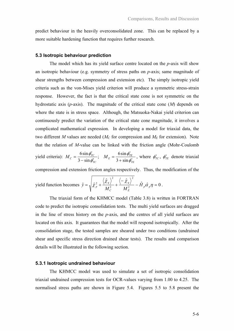
Comparisons, Results and Discussion
5-6
predict behaviour in the heavily overconsolidated zone. This can be replaced by a
more suitable hardening function that requires further research.
5.3 Isotropic behaviour prediction The model which has its yield surface centre located on the p-axis will show
an isotropic behaviour (e.g. symmetry of stress paths on p-axis; same magnitude of
shear strengths between compression and extension etc). The simply isotropic yield
criteria such as the von-Mises yield criterion will produce a symmetric stress-strain
response. However, the fact is that the critical state cone is not symmetric on the
hydrostatic axis (p-axis). The magnitude of the critical state cone (M) depends on
where the state is in stress space. Although, the Matsuoka-Nakai yield criterion can
continuously predict the variation of the critical state cone magnitude, it involves a
complicated mathematical expression. In developing a model for triaxial data, the
two different M values are needed (MC for compression and ME for extension). Note
that the relation of M-value can be linked with the friction angle (Mohr-Coulomb
yield criteria): TE
TEE
TC
TCC MM
φφ
φφ
′+′
=′−
′=
sin3sin6;
sin3sin6
, where TCφ′ , TEφ′ denote triaxial
compression and extension friction angles respectively. Thus, the modification of the
yield function becomes 0ˆˆˆˆ
ˆˆ2
2
2
2
2 =−−
++= ηαχχ
χ ppE
q
C
qp H
MMy .
The triaxial form of the KHMCC model (Table 3.8) is written in FORTRAN
code to predict the isotropic consolidation tests. The multi yield surfaces are dragged
in the line of stress history on the p-axis, and the centres of all yield surfaces are
located on this axis. It guarantees that the model will respond isotropically. After the
consolidation stage, the tested samples are sheared under two conditions (undrained
shear and specific stress direction drained shear tests). The results and comparison
details will be illustrated in the following section.
5.3.1 Isotropic undrained behaviour
The KHMCC model was used to simulate a set of isotropic consolidation
triaxial undrained compression tests for OCR-values varying from 1.00 to 4.25. The
normalised stress paths are shown in Figure 5.4. Figures 5.5 to 5.8 present the

Comparisons, Results and Discussion
5-7
KHMCC model predictions of the isotropic undrained compression tests with OCR
values of 1.00, 1.24, 2.15 and 2.75 respectively. The figures also show a comparison
between the KHMCC model and the MCC model. It shows that the normally
overconsolidated clay (Figure 5.5) is fully predicted by both the MCC model and the
KHMCC model, but the KHMCC model gives a slightly better prediction than the
MCC model. The undrained stress-strain response of normally consolidated clay
exhibits only plastic behaviour because the stress path drags along the yield surface
boundary, which is in the plastic region. Thus, the MCC model can capture this
special behaviour.
0.0
50.0
100.0
150.0
200.0
250.0
300.0
0.0 100.0 200.0 300.0 400.0 500.0 600.0
p (kPa)
q (kPa)
(a)
0.0
50.0
100.0
150.0
200.0
250.0
300.0
0.00 0.05 0.10 0.15 0.20
εs
q (kPa)
(b)
Figure 5.5 Prediction of isotropic consolidation undrained test at OCR = 1.00 (a) Stress path; (b) Shear stress-strain curve
0.0
50.0
100.0
150.0
200.0
250.0
300.0
350.0
400.0
0.0 100.0 200.0 300.0 400.0 500.0 600.0
p (kPa)
q (kPa)
(a)
0.0
50.0
100.0
150.0
200.0
250.0
300.0
350.0
400.0
0.00 0.02 0.04 0.06 0.08 0.10 0.12 0.14 0.16εs
q (kPa)
(b) Figure 5.6 Prediction of isotropic consolidation undrained test at OCR = 1.24
Model
MCC
Data
Model
MCC
Data

Comparisons, Results and Discussion
5-8
(a) Stress path; (b) Shear stress-strain curve
0.0
50.0
100.0
150.0
200.0
250.0
300.0
350.0
400.0
0.0 100.0 200.0 300.0 400.0
p (kPa)
q (kPa)
(a)
0.0
50.0
100.0
150.0
200.0
250.0
300.0
350.0
400.0
0.00 0.02 0.04 0.06 0.08 0.10 0.12 0.14 0.16εs
q (kPa)
(b) Figure 5.7 Prediction of isotropic consolidation undrained test at OCR = 2.15
(a) Stress path; (b) Shear stress-strain curve
0.0
50.0
100.0
150.0
200.0
250.0
300.0
350.0
400.0
0.0 100.0 200.0 300.0 400.0 500.0
p (kPa)
q (kPa)
(a)
0.0
50.0
100.0
150.0
200.0
250.0
300.0
350.0
400.0
0.00 0.02 0.04 0.06 0.08 0.10 0.12 0.14 0.16εs
q (kPa)
(b) Figure 5.8 Prediction of isotropic consolidation undrained test at OCR = 2.75
(a) Stress path; (b) Shear stress-strain curve
On the other hand, the lightly and moderately overconsolidated samples
(Figures 5.6, 5.7 and 5.8) can still use the MCC model to predict their behaviour;
however it does not fit very well for both stress path and stress-strain responses. This
is due to the limitation that the MCC model only gives the elastic response for the
stress state inside the yield surface. The multiple yield surface model can
accommodate the smooth transition change from elastic stiffness to elastic-plastic
Model
MCC
Data
Model
MCC
Data
Comparisons, Results and Discussion
5-9
stiffness. Figures 5.6, 5.7 and 5.8 show that the KHMCC model can capture the
transition of shear stiffness. However, the undrained stress path pattern (Figure 5.4)
does not fit well with all tests, especially heavily overconsolidated samples. This is
because the KHMCC model is strictly based on the CSSM assumption, i.e. every
sheared sample must reach the same final state called “critical state”. The
experimental data, however, did not show a unique critical state. This may be due to
localisation in which each element of the sample does not yield at the same time.
Another way of explaining the phenomenon is the introduction of a strain softening
function, an agenda for further research.
The final version of the KHMCC model cannot accurately give the prediction
of the undrained shear strength especially for the heavily overconsolidated sample.
The most significant advantage over the MCC model is that it can give a smooth
transition of stiffness without any additional expression. This benefit can be applied
for the cyclic loading response, the details of which are in the following section.
5.3.2 Isotropic drained behaviour A set of data for isotropic consolidation triaxial drained tests has been
obtained in the testing program with variation of stress path direction from 0o-360o.
The data are compared with the prediction for the models and some selected results
are presented in Figures 5.9, 5.10 and 5.11. The figures also show a comparison
between the KHMCC model and the MCC model.
The stress history is simplified in the testing program which is illustrated in
Figure 4.4(a). Every sample is in the moderately overconsolidated state (OCR =
2.75) after the isotropic consolidation history path. The samples are then sheared in
the particular direction with strain being controlled. The artificial rate-dependent
process is used for this prediction, using a εµ & value equal to 0.1kPa. This value has a
very small effect on the result following the rate-effect in the consolidation behaviour
prediction section (see Figure 5.1(b)).
Figures 5.9(a) and (b) show the volumetric and shear stress-strain curves of the
CID-56 and CID-236 tests as illustrated by the small diagram. There are three stress-
strain curves, i.e. data, MCC model prediction and KHMCC model prediction.

Comparisons, Results and Discussion
5-10
Figures 5.10(a) and (b) present the volumetric and shear stress-strain curves of the
CID-135 and CID-315 tests.
20.0
40.0
60.0
80.0
100.0
120.0
140.0
160.0
180.0
200.0
-0.100 -0.050 0.000 0.050 0.100 0.150
p(kPa)
εv (-)
(a)
-80.0
-30.0
20.0
70.0
120.0
170.0
-0.10 0.00 0.10 0.20 0.30
εs(-)
q(kPa)
(b) Figure 5.9 Prediction of isotropic consolidation drained test at 56o and 236o direction of
OCR = 2.75; (a) Volumetric stress-strain curve; (b) Shear stress-strain curve
10.0
60.0
110.0
160.0
210.0
-0.100 -0.050 0.000 0.050 0.100 0.150
p(kPa)
εv (-)
(a)
-180.0
-130.0
-80.0
-30.0
20.0
-0.18 -0.13 -0.08 -0.03 0.02 0.07εs(-)
q(kPa)
(b) Figure 5.10 Prediction of isotropic consolidation drained test at 135o and 315o direction of
OCR = 2.75; (a) Volumetric stress-strain curve; (b) Shear stress-strain curve
135o
315o
56o
236o
Model
MCC
Data
Model
MCC
Data
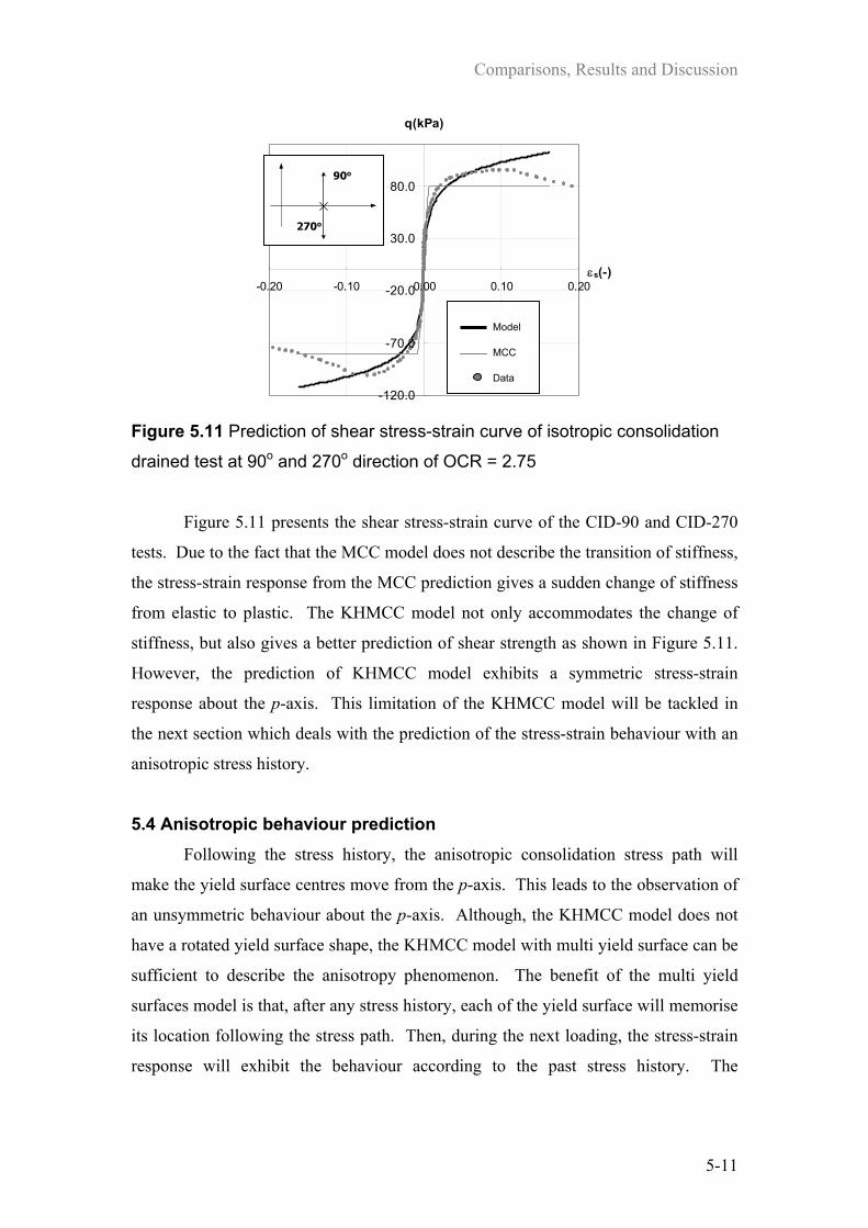
Comparisons, Results and Discussion
5-11
-120.0
-70.0
-20.0
30.0
80.0
-0.20 -0.10 0.00 0.10 0.20εs(-)
q(kPa)
Figure 5.11 Prediction of shear stress-strain curve of isotropic consolidation
drained test at 90o and 270o direction of OCR = 2.75
Figure 5.11 presents the shear stress-strain curve of the CID-90 and CID-270
tests. Due to the fact that the MCC model does not describe the transition of stiffness,
the stress-strain response from the MCC prediction gives a sudden change of stiffness
from elastic to plastic. The KHMCC model not only accommodates the change of
stiffness, but also gives a better prediction of shear strength as shown in Figure 5.11.
However, the prediction of KHMCC model exhibits a symmetric stress-strain
response about the p-axis. This limitation of the KHMCC model will be tackled in
the next section which deals with the prediction of the stress-strain behaviour with an
anisotropic stress history.
5.4 Anisotropic behaviour prediction Following the stress history, the anisotropic consolidation stress path will
make the yield surface centres move from the p-axis. This leads to the observation of
an unsymmetric behaviour about the p-axis. Although, the KHMCC model does not
have a rotated yield surface shape, the KHMCC model with multi yield surface can be
sufficient to describe the anisotropy phenomenon. The benefit of the multi yield
surfaces model is that, after any stress history, each of the yield surface will memorise
its location following the stress path. Then, during the next loading, the stress-strain
response will exhibit the behaviour according to the past stress history. The
90o
270o
Model
MCC
Data

Comparisons, Results and Discussion
5-12
prediction of the shear strength can be improved using the inequality of critical state
cone magnitude (M). In this stage, however, the two different M values are used for
the triaxial model (in p-q space).
Incorporating the KHMCC model (Table 3.8) into the FORTRAN code, the
prediction of anisotropic consolidation tests is processed. Firstly, the multi yield
surfaces are dragged following the anisotropic consolidation stress history as shown in
Figure 4.5. After the consolidation stage, the tested samples are sheared into two
conditions (undrained shear condition and some specific stress direction drained shear
condition). The results and comparison details will be described in the following
section.
0.00
0.10
0.20
0.30
0.40
0.50
0.60
0.70
0.80
0.90
1.00
0.00 0.20 0.40 0.60 0.80 1.00 1.20p/pmax
q/pmax
Figure 5.12 Prediction of K0 consolidation
undrained compression shear stress paths varying
OCR from 1.00 to 2.75
-1.20
-1.00
-0.80
-0.60
-0.40
-0.20
0.00
0.20
0.40
0.60
0.00 0.20 0.40 0.60 0.80 1.00 1.20
p/pmax
q/pmax
Figure 5.13 Prediction of K0 consolidation
undrained extension shear stress paths varying
OCR from 1.00 to 2.75
5.4.1 Anisotropic undrained behaviour The KHMCC model is used to simulate two sets of K0 consolidation triaxial
undrained tests with varying OCR-values from 1.00 to 2.75, both in compression and
extension tests. The normalised stress paths are shown in Figures 5.12 and 5.13 for
compression and extension tests respectively. Figures 5.14 to 5.17 present the model
predictions of the K0 undrained compression tests with OCR values 1.00, 1.24, 2.15
CS Line
Model
Data
CS Line
Model
Data

Comparisons, Results and Discussion
5-13
and 2.75 respectively, and Figures 5.18 to 5.21 exhibit the model predictions of the K0
undrained extension tests with varying the OCR values 1.00, 1.24, 2.15 and 2.75
respectively. These plots show the comparison between the experimental data, the
MCC model and the KHMCC model prediction.
0
50
100
150
200
250
300
350
0 100 200 300 400 500p (kPa)
q (kPa)
(a)
200
220
240
260
280
300
320
340
0.00 0.02 0.04 0.06 0.08 0.10 0.12εs (-)
q (kPa)
(b)
Figure 5.14 Prediction of K0 consolidation undrained compression test at OCR = 1.00
(a) Stress path; (b) Shear stress-strain curve
0
50
100
150
200
250
300
350
0 100 200 300 400 500p (kPa)
q (kPa)
(a)
200
220
240
260
280
300
320
0.00 0.02 0.04 0.06 0.08 0.10 0.12εs (-)
q (kPa)
(b)
Figure 5.15 Prediction of K0 consolidation undrained compression test at OCR = 1.24
(a) Stress path; (b) Shear stress-strain curve
Model
MCC
Data
Model
MCC
Data
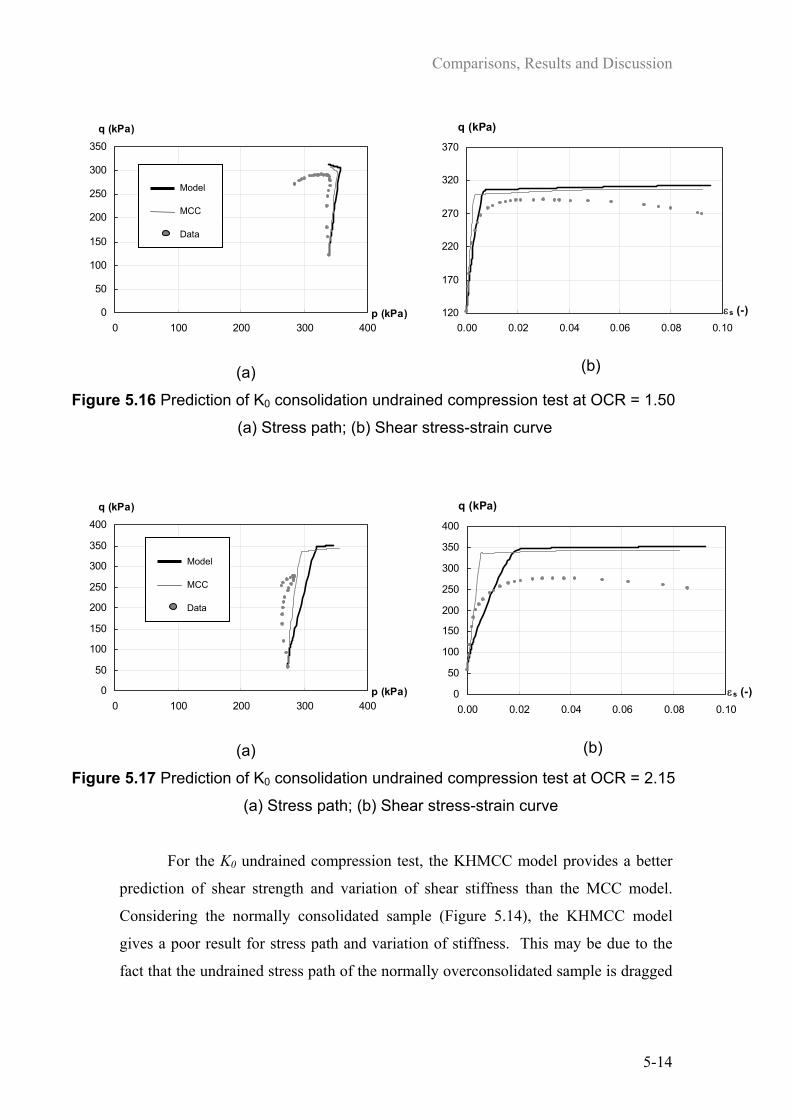
Comparisons, Results and Discussion
5-14
0
50
100
150
200
250
300
350
0 100 200 300 400p (kPa)
q (kPa)
(a)
120
170
220
270
320
370
0.00 0.02 0.04 0.06 0.08 0.10
εs (-)
q (kPa)
(b)
Figure 5.16 Prediction of K0 consolidation undrained compression test at OCR = 1.50
(a) Stress path; (b) Shear stress-strain curve
0
50
100
150
200
250
300
350
400
0 100 200 300 400p (kPa)
q (kPa)
(a)
0
50
100
150
200
250
300
350
400
0.00 0.02 0.04 0.06 0.08 0.10εs (-)
q (kPa)
(b)
Figure 5.17 Prediction of K0 consolidation undrained compression test at OCR = 2.15
(a) Stress path; (b) Shear stress-strain curve
For the K0 undrained compression test, the KHMCC model provides a better
prediction of shear strength and variation of shear stiffness than the MCC model.
Considering the normally consolidated sample (Figure 5.14), the KHMCC model
gives a poor result for stress path and variation of stiffness. This may be due to the
fact that the undrained stress path of the normally overconsolidated sample is dragged
Model
MCC
Data
Model
MCC
Data
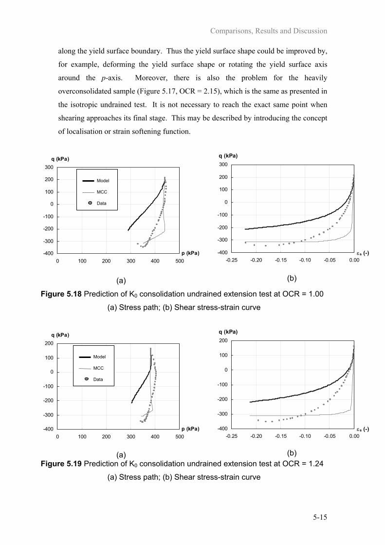
Comparisons, Results and Discussion
5-15
along the yield surface boundary. Thus the yield surface shape could be improved by,
for example, deforming the yield surface shape or rotating the yield surface axis
around the p-axis. Moreover, there is also the problem for the heavily
overconsolidated sample (Figure 5.17, OCR = 2.15), which is the same as presented in
the isotropic undrained test. It is not necessary to reach the exact same point when
shearing approaches its final stage. This may be described by introducing the concept
of localisation or strain softening function.
-400
-300
-200
-100
0
100
200
300
0 100 200 300 400 500p (kPa)
q (kPa)
(a)
-400
-300
-200
-100
0
100
200
300
-0.25 -0.20 -0.15 -0.10 -0.05 0.00εs (-)
q (kPa)
(b)
Figure 5.18 Prediction of K0 consolidation undrained extension test at OCR = 1.00
(a) Stress path; (b) Shear stress-strain curve
-400
-300
-200
-100
0
100
200
0 100 200 300 400 500p (kPa)
q (kPa)
(a)
-400
-300
-200
-100
0
100
200
-0.25 -0.20 -0.15 -0.10 -0.05 0.00εs (-)
q (kPa)
(b) Figure 5.19 Prediction of K0 consolidation undrained extension test at OCR = 1.24
(a) Stress path; (b) Shear stress-strain curve
Model
MCC
Data
Model
MCC
Data

Comparisons, Results and Discussion
5-16
-350-300
-250-200-150-100
-500
50
100150
0 100 200 300 400p (kPa)
q (kPa)
(a)
-350
-300
-250
-200
-150
-100
-50
0
50
100
150
-0.20 -0.15 -0.10 -0.05 0.00εs (-)
q (kPa)
(b)
Figure 5.20 Prediction of K0 consolidation undrained extension test at OCR = 1.78
(a) Stress path; (b) Shear stress-strain curve
-400-350
-300-250-200-150
-100-50
0
50100
0 100 200 300 400p (kPa)
q (kPa)
(a)
-400
-350
-300
-250
-200
-150
-100
-50
0
50
100
-0.25 -0.20 -0.15 -0.10 -0.05 0.00εs (-)
q (kPa)
(b)
Figure 5.21 Prediction of K0 consolidation undrained extension test at OCR = 2.15
(a) Stress path; (b) Shear stress-strain curve
For the K0 undrained extension test, the prediction exhibits the same trend as
the compression tests except for the prediction of shear strength. The KHMCC model
underestimates the shear strength value, compared to the MCC model. This may be
due to the effect of the M-value, i.e. MC is more than ME, when keeping TCφ′ = TEφ′ as a
Model
MCC
Data
Model
MCC
Data

Comparisons, Results and Discussion
5-17
material constant. However, this seems to be unsuitable for the explanation of the
experimental data from AIT because the data shows that the extension shear strength
is slightly higher than the compression shear strength. The KHMCC model allows the
use of the same M-value for both compression and extension, MC = ME (as shown in
Table 5.1). The prediction of shear stiffness on the extension side is reasonably
accurate, compared with the compression side. This simplification to the model
reasonably compensates for the shortfall of the model.
5.4.2 Anisotropic drained behaviour Like the isotropic consolidation data, the data for the anisotropic consolidation
triaxial drained test are provided by the varying stress path directions from 0o-360o.
Figures 5.22 to 5.25 show the comparison of the prediction of the KHMCC model and
the MCC model with experimental data from AIT. Figures 5.22(a) and (b) show the
volumetric and shear stress-strain curves of the CKD-45 and CKD-225 tests as shown
in the small diagram. Figures 5.23(a) and (b) present the similar curves of CKD-135
and CKD-315 tests. Figures 5.24(a) and (b) exhibit the volumetric stress-strain plots
of CKD-0 and CKD-180 tests respectively; on the other hand, Figure 5.25 presents the
shear stress-strain curve of CKD-90 and CKD-270 tests.
0
20
40
60
80
100
120
140
160
180
-0.100 -0.050 0.000 0.050 0.100
p (kPa)
εv (-)
(a)
-50
-30
-10
10
30
50
70
90
110
130
150
-0.150 -0.100 -0.050 0.000 0.050 0.100 0.150εs(-)
q (kPa)
(b)
Figure 5.22 Prediction of K0 consolidation drained test at 45o and 225o direction
of OCR = 2.75; (a) Volumetric stress-strain curve; (b) Shear stress-strain curve
45o
225o Model
MCC
Data

Comparisons, Results and Discussion
5-18
20
40
60
80
100
120
140
160
180
200
220
-0.100 0.000 0.100 0.200
p (kPa)
εv (-)
(a)
-130
-110
-90
-70
-50
-30
-10
10
30
50
-0.280 -0.180 -0.080 0.020 0.120εs(-)
q (kPa)
(b) Figure 5.23 Prediction of K0 consolidation drained test at 135o and 315o direction
of OCR = 2.75; (a) Volumetric stress-strain curve; (b) Shear stress-strain curve
60
160
260
360
460
560
660
0.000 0.050 0.100 0.150 0.200 0.250 0.300 0.350
p (kPa)
εv (-)
(a)
0
10
20
30
40
50
60
-0.060 -0.050 -0.040 -0.030 -0.020 -0.010 0.000
p (kPa)
εv (-)
(b)
Figure 5.24 Prediction of volumetric stress-strain curve of K0 consolidation drained test
of OCR = 2.75; (a) 0o direction; (b) 180o direction
135o
315o
0o180o Model
MCC
Data
Model
MCC
Data
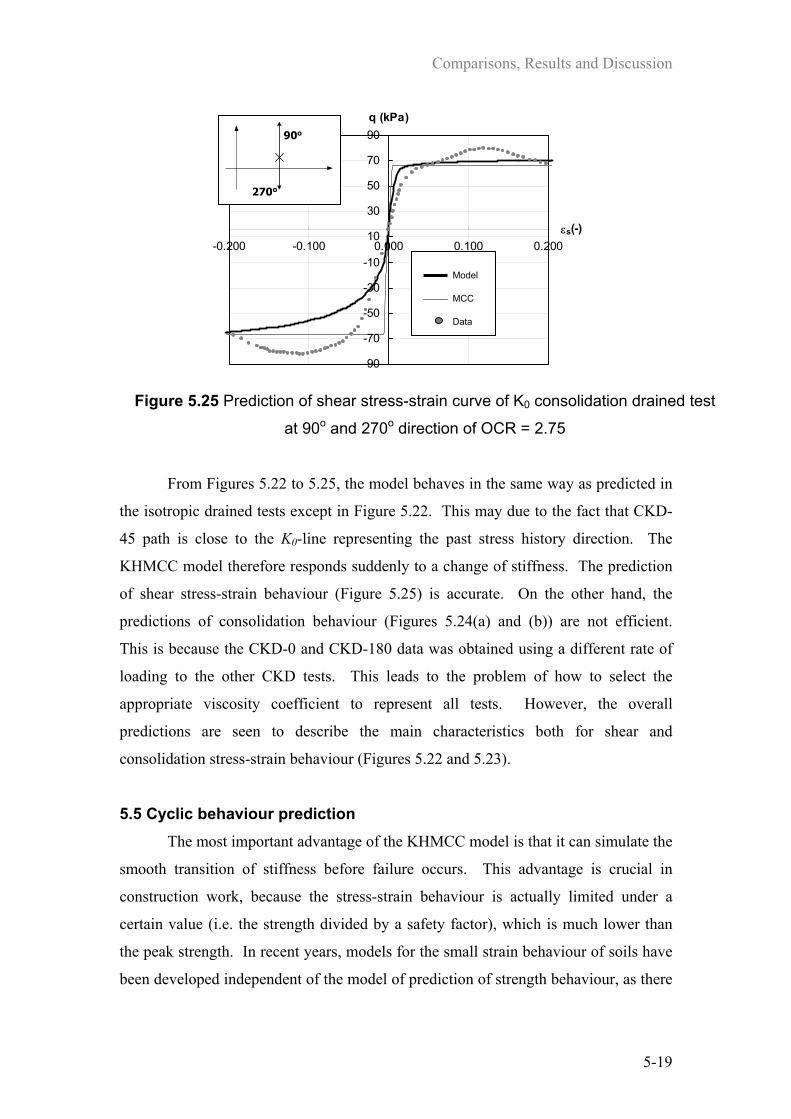
Comparisons, Results and Discussion
5-19
-90
-70
-50
-30
-10
10
30
50
70
90
-0.200 -0.100 0.000 0.100 0.200εs(-)
q (kPa)
Figure 5.25 Prediction of shear stress-strain curve of K0 consolidation drained test
at 90o and 270o direction of OCR = 2.75
From Figures 5.22 to 5.25, the model behaves in the same way as predicted in
the isotropic drained tests except in Figure 5.22. This may due to the fact that CKD-
45 path is close to the K0-line representing the past stress history direction. The
KHMCC model therefore responds suddenly to a change of stiffness. The prediction
of shear stress-strain behaviour (Figure 5.25) is accurate. On the other hand, the
predictions of consolidation behaviour (Figures 5.24(a) and (b)) are not efficient.
This is because the CKD-0 and CKD-180 data was obtained using a different rate of
loading to the other CKD tests. This leads to the problem of how to select the
appropriate viscosity coefficient to represent all tests. However, the overall
predictions are seen to describe the main characteristics both for shear and
consolidation stress-strain behaviour (Figures 5.22 and 5.23).
5.5 Cyclic behaviour prediction The most important advantage of the KHMCC model is that it can simulate the
smooth transition of stiffness before failure occurs. This advantage is crucial in
construction work, because the stress-strain behaviour is actually limited under a
certain value (i.e. the strength divided by a safety factor), which is much lower than
the peak strength. In recent years, models for the small strain behaviour of soils have
been developed independent of the model of prediction of strength behaviour, as there
90o
270o
Model
MCC
Data
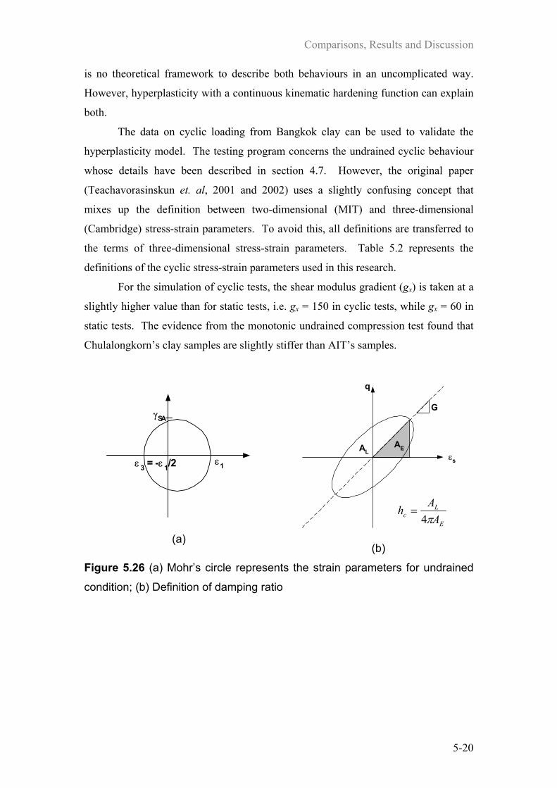
Comparisons, Results and Discussion
5-20
is no theoretical framework to describe both behaviours in an uncomplicated way.
However, hyperplasticity with a continuous kinematic hardening function can explain
both.
The data on cyclic loading from Bangkok clay can be used to validate the
hyperplasticity model. The testing program concerns the undrained cyclic behaviour
whose details have been described in section 4.7. However, the original paper
(Teachavorasinskun et. al, 2001 and 2002) uses a slightly confusing concept that
mixes up the definition between two-dimensional (MIT) and three-dimensional
(Cambridge) stress-strain parameters. To avoid this, all definitions are transferred to
the terms of three-dimensional stress-strain parameters. Table 5.2 represents the
definitions of the cyclic stress-strain parameters used in this research.
For the simulation of cyclic tests, the shear modulus gradient (gx) is taken at a
slightly higher value than for static tests, i.e. gx = 150 in cyclic tests, while gx = 60 in
static tests. The evidence from the monotonic undrained compression test found that
Chulalongkorn’s clay samples are slightly stiffer than AIT’s samples.
ε 3 = -ε 1/2 ε1
γSA
(a)
AEAL
G
q
εs
(b)
Figure 5.26 (a) Mohr’s circle represents the strain parameters for undrained
condition; (b) Definition of damping ratio
E
Lc A
Ahπ4
=

Comparisons, Results and Discussion
5-21
Table 5.2 The definitions of cyclic stress-strain parameters
Definition Description
( )22
31 εεγ −=SA ; in undrained condition sSA εγ 5.1= Single amplitude shear strain
( )ν−=
12EG ; in undrained condition
s
qGε
= Secant shear modulus
E
Lc A
Ahπ4
= ; where LA and EA represent the area of
hysterisis loop and the area of elastic zone (show in
Figure 5.26)
Damping ratio
Figures 5.27 and 5.28 present the simulated result of cyclic undrained shear
tests with varying confining pressure (pc) of 50 and 100kPa respectively. The results
exhibit the variation of shear modulus and damping ratio with single amplitude shear
strain. The prediction of cyclic undrained triaxial tests are good for both the normally
consolidated sample (pc = 100kPa) and lightly overconsolidated sample (pc = 50kPa).
The N-value in Figures 5.27 and 5.28 represent the number of testing cycles.
Although, the testing program has not been continued until failure (excess pore
pressure develops due to the cyclic load), the first ten cycles are sufficient to represent
the cyclic behaviour. The effect of viscous behaviour on cyclic properties can
actually be investigated by the KHMCC model. However, because of the
inconsiderable amount of the frequency difference in the data, it does not show a
significant effect.
The prediction of the cyclic test at small strains is the most important
advantage of the multiple yield surface model. In particular, the rate-dependent
model shows the deformed elliptical shape of hysteresis loops during the cyclic load.
The area of the hysteresis loop becomes larger when the number of cycles increases.
This evidence is exhibited on the damping ratio Figures 5.27(b) and 5.28(b).

Comparisons, Results and Discussion
5-22
0
12
34
56
78
9
0.0001 0.0010 0.0100 0.1000 1.0000
γ(−)
G (MPa)
0.24 (data) N=23700.40 (data) N=3500.60 (data) N=2130.24 (model) N=100.40 (model) N=100.60 (model) N=10
(a)
0
5
10
15
20
25
30
0.0001 0.0010 0.0100 0.1000 1.0000
γ(−)
h c (%)
(b)
Figure 5.27 Prediction of cyclic undrained shear test varying shear stress
magnitude (q/p) at confining pressure (pc) = 50kPa, N = number of cycles
(a) Plot of shear modulus (G) vs. single amplitude shear strain ( SAγ )
(b) Plot of damping ratio ( ch ) vs. single amplitude shear strain ( SAγ )

Comparisons, Results and Discussion
5-23
0123456789
10
0.0010 0.0100 0.1000 1.0000
γ(−)
G (MPa)
0.32 (data) N=234600.56 (data) N=53600.80 (data) N=6530.32 (model) N=100.56 (model) N=100.80 (model) N=10
(a)
0
5
10
15
20
25
30
35
40
45
50
0.0010 0.0100 0.1000 1.0000
γ(−)
h c (%)
(b)
Figure 5.28 Prediction of cyclic undrained shear test varying shear stress
magnitude (q/p) at confining pressure (pc) = 100kPa, N = number of cycles
(c) Plot of shear modulus (G) vs. single amplitude shear strain ( SAγ )
(d) Plot of damping ratio ( ch ) vs. single amplitude shear strain ( SAγ )
Comparisons, Results and Discussion
5-24
5.6 Conclusion and Future work The hyperplasticity model based on two potential functions can define the
constitutive law for an engineering material, especially soil. The advantage is that a
continuous kinematic hardening function can exhibit a continuous stress-strain
response. The KHMCC model with a linear stress-strain relationship has been finally
proposed for the implementation. A parametric study on Bangkok clay is based on
two sources of research. All predictions of the experimental result have been
processed by FORTAN 90 with the assumption that stress-strain is uniformly
distributed under the triaxial condition (axi-symmetry condition). Every sample is
consolidated following its stress history and sheared in its specific condition such as
undrained, drained or cyclic undrained condition.
The prediction for consolidation behaviour is more accurate than shear
behaviour. Since, the consolidation prediction only acts on the p term of the model,
there is no p-q coupling term that affects the stress-strain response. The real-time
analysis can be done by means of adjusting the viscosity coefficient and the rate in the
rate-dependent analysis.
The prediction for pure shear behaviour can be determined from the CID-90
and CID-270 tests. These two tests are used to evaluate the magnitude of the critical
state cone both on the compression and extension sides. The evidence on anisotropic
tests, however, shows that the extension strength is slightly higher than compression.
Thus, for simplicity for the downside of the model, the assumption that EC MM = has
been proposed in this study.
The isotropic consolidated tests are accurately predicted in terms of stress path
and shear strength. On the other hand, the anisotropic consolidated samples are
slightly inaccurate, especially the stress path. The variation of shear stiffness is
relatively well fitted for both isotropic and anisotropic consolidated tests. However,
the prediction of the shear strength of the heavily overconsolidated sample should be
improved.
The simulation of the cyclic undrained tests gives an accurate result. The
variation of the shear modulus is simulated by the model accurately all shear strain
amplitudes. The damping ratio is also well predicted at all shear strain amplitudes.
Comparisons, Results and Discussion
5-25
This leads to the significant benefit of the model that it can simulate both the
monotonic loading and the cyclic loading behaviour by a unique constitutive law.
However, this version of the hyperplasticity model still has to be improved.
The suggested information is summarised below:
1. Because the model is based strictly on the Masing rule; it always gives a
symmetric closed hysteresis loop when the stress path returns to the same maximum
past stress. Further research has to introduce a ratchetting mechanism that will
provide an unsymmetrical hysteresis loop and a small drift after one load cycle.
2. The investigation shows that it is not necessary to strictly enforce the CSSM
assumption that every sheared sample must reach the same critical state. Further
research should consider either the concept of localisation or the strain softening
phenomenon. The localisation idea assumes that material consists of two zones i.e.
elastic and plastic zones3, where the ratio of these two zone’s volume controls the
material behaviour. This idea implies that all material elements do not necessarily
reach the yield state at the same time. In contrast, the strain softening will result in a
softening behaviour after material yield. The yield surface will move inward or
shrink when the stress state touches the yield surface. These two concepts might be
used to explain the behaviour of heavily overconsolidated clay.
3. The fact that the magnitude of the critical state cone (M) depends on where
the stress state is in stress space. For the generalised stress-strain model, the general
expression to evaluate the shape of critical state cone has to be considered.
4. For the better prediction of anisotropy, the yield surface shape may be
improved by, for example, deforming the yield surface shape or rotating the yield
surface axis around the p-axis. These ideas are believed to be able to generate
anisotropy.
3 the plastic zone is sometimes called the shear band

Implementation into finite element code
6-1
Chapter 6 Implementation into Finite Element Code
In recent times, the finite element method has been used in engineering
practice including for the analysis of geotechnical problems. A finite element
program OXFEM has been developed at the University of Oxford over the last ten
years. The nested yield surface model, a multi yield surface soil model, has been
implemented into OXFEM (Augarde, 1997). Based on the hyperplasticity approach
(Collins and Houlsby, 1997, and Houlsby and Puzrin, 2000), rate independent
plasticity is not difficult apply in OXFEM. Nonetheless, the rate-dependent
calculation is distinctively different from the classical plasticity theory. The rate-
dependent stress-strain algorithm must be further developed and included in the
OXFEM code.
This chapter focuses on the implementation of the new constitutive law using
the finite element method, and the two-dimensional finite element formulation for
geotechnical problems is summarised. The KHMCC and MCC models are
represented in terms of generalised stress-strain parameters. The models are also
reduced for the analysis of the two-dimensional problem.
6.1 Stress-strain definition The formulation of an element stiffness matrix is based on the isoparametric
method used in the derivation of small strain finite element equations. If
deformations are defined by continuous functions u, v and w in the x, y and z
directions respectively, the strains (assuming small strain theory and a compression
positive sign convention) are defined as (Howatson, Lund and Todd, 1991):
zw
yv
xu
zyx ∂∂
−=∂∂
−=∂∂
−= εεε ;;
zu
xw
zv
yw
yu
xv
xzyzxy ∂∂
−∂∂
−=∂∂
−∂∂
−=∂∂
−∂∂
−= γγγ ;; (6.1)
As the six strains are a function of only three displacements, they are not independent.
However, to analyse a real geotechnical problem, some assumptions and
idealisations must be made. Due to the special geometric characteristics of many
problems such as retaining walls, continuous footings and stability of slopes, they can
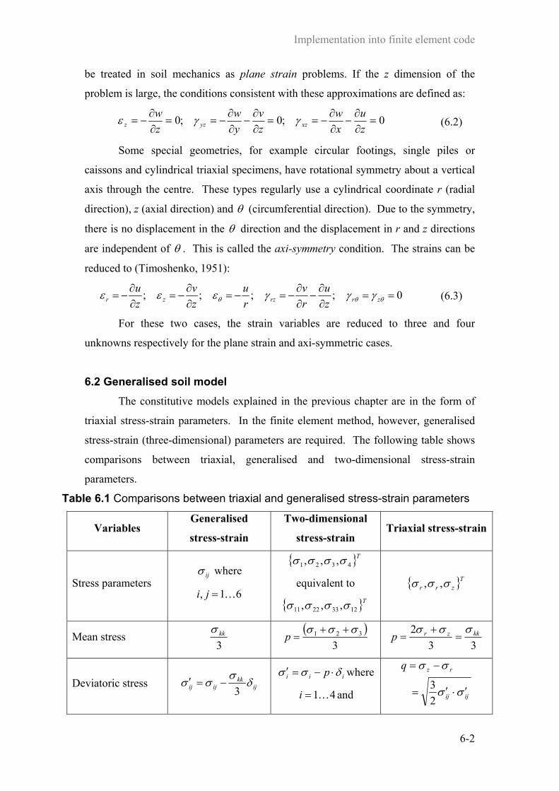
Implementation into finite element code
6-2
be treated in soil mechanics as plane strain problems. If the z dimension of the
problem is large, the conditions consistent with these approximations are defined as:
0;0;0 =∂∂
−∂∂
−==∂∂
−∂∂
−==∂∂
−=zu
xw
zv
yw
zw
xzyzz γγε (6.2)
Some special geometries, for example circular footings, single piles or
caissons and cylindrical triaxial specimens, have rotational symmetry about a vertical
axis through the centre. These types regularly use a cylindrical coordinate r (radial
direction), z (axial direction) and θ (circumferential direction). Due to the symmetry,
there is no displacement in the θ direction and the displacement in r and z directions
are independent of θ . This is called the axi-symmetry condition. The strains can be
reduced to (Timoshenko, 1951):
0;;;; ==∂∂
−∂∂
−=−=∂∂
−=∂∂
−= θθθ γγγεεε zrrzzr zu
rv
ru
zv
zu (6.3)
For these two cases, the strain variables are reduced to three and four
unknowns respectively for the plane strain and axi-symmetric cases.
6.2 Generalised soil model The constitutive models explained in the previous chapter are in the form of
triaxial stress-strain parameters. In the finite element method, however, generalised
stress-strain (three-dimensional) parameters are required. The following table shows
comparisons between triaxial, generalised and two-dimensional stress-strain
parameters.
Table 6.1 Comparisons between triaxial and generalised stress-strain parameters
Variables Generalised
stress-strain
Two-dimensional
stress-strain Triaxial stress-strain
Stress parameters ijσ where
61, K=ji
{ }T4321 ,,, σσσσ
equivalent to
{ }T12332211 ,,, σσσσ
{ }Tzrr σσσ ,,
Mean stress 3kkσ
( )3
321 σσσ ++=p
332 kkzrp
σσσ=
+=
Deviatoric stress ijkk
ijij δσ
σσ3
−=′ iii p δσσ ⋅−=′ where
41K=i and ijij
rzq
σσ
σσ
′⋅′=
−=
23

Implementation into finite element code
6-3
=−=
=40
31,1i
iiδ
Strain parameters ijε where
61, K=ji
{ }T4321 ,,, εεεε
equivalent to
{ }T12332211 2,,, εεεε
{ }Tzrr εεε ,,
Volumetric strain kkε 321 εεεε ++=v kkzrv εεεε =+= 2
Deviatoric strain ijkk
ijij δε
εε3
−=′ iiiv δεε3
−=′ where
41K=i
( )
ijij
rzs
εε
εεε
′⋅′=
−=
32
32
Bulk modulus (K) kk
kkKεσ
=3 v
pKε
= v
pKε
=
Shear modulus (G) ij
ijGεσ′
′=2
i
iGεσ′′
=2 s
qGε
=3
The MCC model and KHMCC model can be transformed into the generalised stress-
strain parameters shown in Table 6.2. The simplicity of the generalisation from
triaxial conditions is a feature of the approach in which the model is defined entirely
by scalar functions.
Table 6.2 Generalised soil models
MCC model
( )
−⋅⋅−+−
′′⋅−
⋅−=
κλασ
κλασσσσ
σσσ
κ kkkkijij
kkx
ijij
kk
kkkk
gg exp
343ilog
30
0
20
0exp32
39
02
2
=
−⋅−
′′⋅+=
κλασχχχ kkkkxijijkk
My
where subscript 0, x represent the reference (initial) and the reference point
of yield surface
KHMCC model
∫
′′++−
′′⋅−−=
1
0
22
3ˆˆˆ
2ˆˆ
43
18η
αααασ
σσσσ
dHH
gKg ijijqkkp
ijijkkx
ijijkk
0ˆˆˆˆ23
9ˆ
ˆ2
2
=−′′
⋅+= ηαχχχ
kkpijijkk H
My

Implementation into finite element code
6-4
6.3 Two-dimensional soil model for OXFEM Taking advantage of the special geometry arising in many geotechnical
problems, some assumptions are made to reduce the amount of calculation in the
finite element analysis. In this research, the two-dimensional analysis, such as plane
strain and/or axi-symmetry is used. However, a transformation from generalised
stress-strain parameters to two-dimensional stress-strain parameters is required and is
shown in Table 6.2. The two-dimensional version of the MCC model and KHMCC
model defined by two scalar functions is presented in Table 6.3.
Table 6.3 Two-dimensional soil models
MCC model
( )( )
( )
−⋅⋅−+
⋅+⋅−
′+′⋅−
⋅−=
∑∑
∑∑
∑
∑
∑∑
==
=
=
=
=
==
κλ
ασκλ
ασασ
σ
σσ
σ
σσκ
3
1
3
10
3
1
443
1
24
3
1
2
3
10
3
1
3
10
exp3
22
2
43ilog
3
ii
iix
iii
iix
ii
ii
ii
ii
gg
( )0exp
3
2
23
9
3
1
3
10
2
24
3
1
223
1 =
−⋅−
′+′⋅+
=∑∑∑∑====
κλ
ασχχχi
ii
ixi
ii
i
My
KHMCC model
( )( )
( )∫
∑∑
∑∑
∑∑
′
+′
+
+
⋅+⋅−
′+′⋅−
−=
==
=
=
==
1
0
24
3
1
223
1
3
1
443
1
24
3
1
223
1
3
2ˆ
2ˆˆ
2
ˆˆ
22
2
43
18
η
ααα
ασασ
σ
σσσ
d
HH
gK
g
iiq
iip
iii
iix
ii
ii
( )0ˆˆ
ˆ2ˆ
23
9
ˆˆ
3
12
24
3
1
223
1 =⋅
−
′+′⋅+
= ∑∑∑
=
== ηαχχχ
iip
ii
ii
HM
y

Implementation into finite element code
6-5
6.4 Solution scheme There are two levels for the calculation of the stress-strain relationship, i.e. the
incremental stress-strain for each single element, and the incremental load-
deformation behaviour of the global problem. The former calculation uses exactly the
same algorithm as in the case of the triaixal stress-strain calculation explained in
chapter 3. The latter one, on the other hand, has to deal with a slightly more
complicated situation, which will be discussed in this section.
6.4.1 Incremental stress-strain solution at element level
The incremental stress-strain solution at the element level is still based on rate-
dependent calculations mentioned in section 3.9.3. However, there exists no
requirement for a constraint statement during the finite element calculation. The
incremental response can be rewritten in the form:
dtdwgddg
jjiij
ji
∂∂
⋅∂∂
∂+=
∂∂∂
− ∫ ηχασ
εσσσ ˆˆ
ˆˆ 22
(6.4)
or, in the matrix form: ( ){ }dtd∫ ⋅−=⋅ ηCBdεdσA (6.5)
where ji
gσσ ∂∂
∂−=
ˆ2
A , ji
gασ ˆˆ2
∂∂∂
−=B , and j
wχ∂∂
=C .
The incremental stress can be solved from equation 6.5 in the form
( ){ }( )dtd∫ ⋅−⋅= − ηCBdεAdσ 1 . Compared with the formulation of the elasto-plastic
constitutive matrix, the relation between incremental stress and incremental strain
takes the form ( )pdεdεDdσ −⋅= , where D or 1A− represents the purely elastic
stiffness matrix.
6.4.2 Modified Newton-Raphson (MNR) method Commonly, the analysis of any boundary value problems can be expressed by
the governing finite element equations which can be reduced to the following
incremental form: iii
GnGG ∆f∆dK =⋅ (6.6)
where iGK is the incremental global stiffness matrix, i
nG∆d is the vector of
incremental nodal displacements, iG∆f is the vector of incremental nodal forces and

Implementation into finite element code
6-6
superscript i is the increment number. To obtain a solution to the boundary value
problem, the change in boundary conditions is normally applied in the form of a series
of increments, in which the governing equation of each increment must be solved.
The final solution is obtained by summing the results of each increment. Normally,
the incremental global stiffness matrix iGK depends on the current stress and strain
level and therefore is not constant, except in the linear elasticity case. If sufficiently
small increments are used, the integration of piecewise linear increments represents
non-linear constitutive behaviour. There are several strategies to solve the non-linear
governing equation. However, only two categories of solution algorithm are
considered: the Euler scheme and Newton-Raphson (NR) scheme (Burd, 1986).
The simplest solution strategy is the Euler scheme, also called the tangential
stiffness method. According to this approach, the incremental stiffness matrix is
assumed constant over each increment and is calculated by using the current state
from the beginning of each increment (i.e. iGK is calculated by using i
nG∆d ). This is
equivalent to making a piecewise linear approximation to the non-linear constitutive
behaviour as illustrated in Figure 6.1(a). Explicitly, the accuracy of the solution
depends on the size of load increments. For example, if the increment size was
reduced so that more increments were needed to reach the same accumulated load, the
tangent stiffness solution would be nearer to the true solution.
Force
Displacement
∆f1
∆f2
∆f3
True solution
Euler scheme
∆dnG1 ∆dnG
3
∆dnG2
KG1
KG3
KG2
(a)
Force
Displacement
∆f1
∆f2
∆f3
True solution
Newton-Raphson scheme
∆dnG1 ∆dnG
3∆dnG2
(b)
Figure 6.1 Solution schemes for Finite Element Analysis;
(a) Euler scheme, (b) Newton-Raphson (NR) scheme
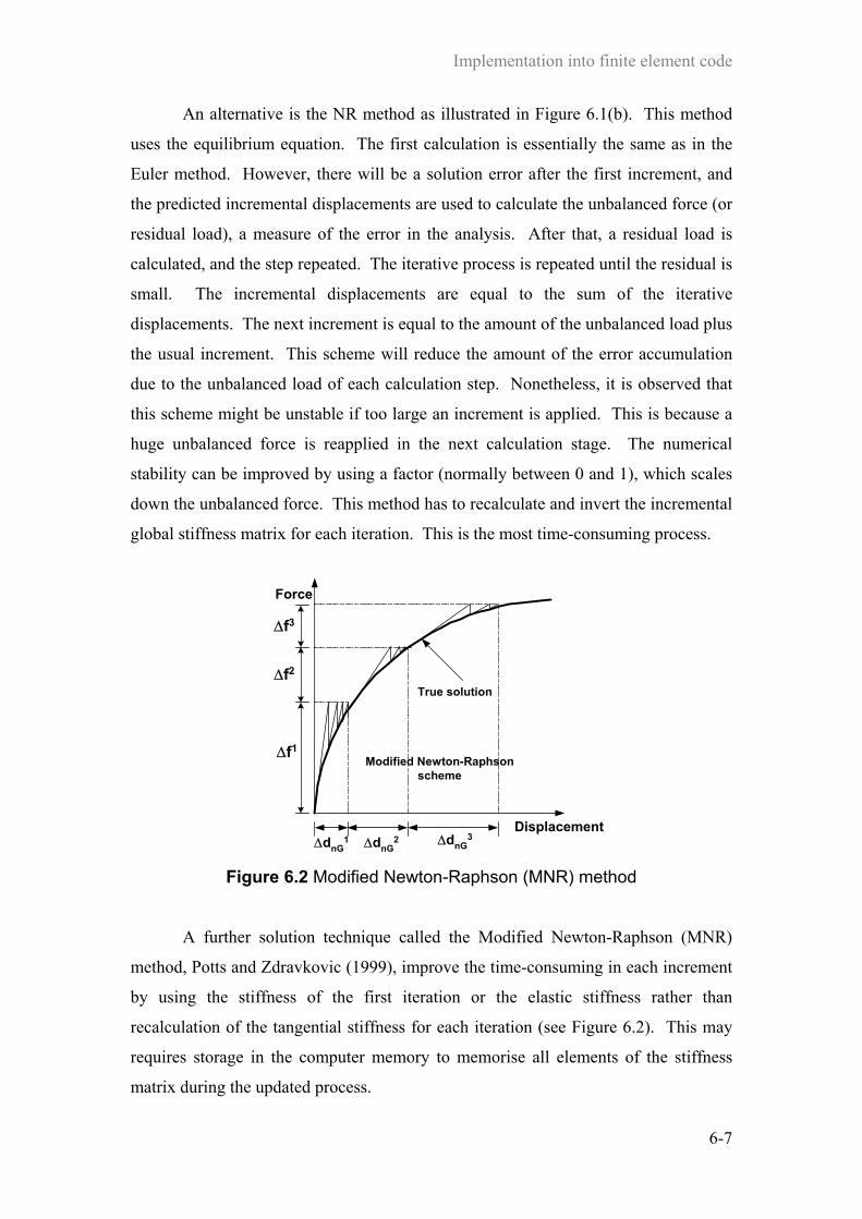
Implementation into finite element code
6-7
An alternative is the NR method as illustrated in Figure 6.1(b). This method
uses the equilibrium equation. The first calculation is essentially the same as in the
Euler method. However, there will be a solution error after the first increment, and
the predicted incremental displacements are used to calculate the unbalanced force (or
residual load), a measure of the error in the analysis. After that, a residual load is
calculated, and the step repeated. The iterative process is repeated until the residual is
small. The incremental displacements are equal to the sum of the iterative
displacements. The next increment is equal to the amount of the unbalanced load plus
the usual increment. This scheme will reduce the amount of the error accumulation
due to the unbalanced load of each calculation step. Nonetheless, it is observed that
this scheme might be unstable if too large an increment is applied. This is because a
huge unbalanced force is reapplied in the next calculation stage. The numerical
stability can be improved by using a factor (normally between 0 and 1), which scales
down the unbalanced force. This method has to recalculate and invert the incremental
global stiffness matrix for each iteration. This is the most time-consuming process.
Force
Displacement
∆f1
∆f2
∆f3
True solution
Modified Newton-Raphsonscheme
∆dnG1 ∆dnG
3∆dnG2
Figure 6.2 Modified Newton-Raphson (MNR) method
A further solution technique called the Modified Newton-Raphson (MNR)
method, Potts and Zdravkovic (1999), improve the time-consuming in each increment
by using the stiffness of the first iteration or the elastic stiffness rather than
recalculation of the tangential stiffness for each iteration (see Figure 6.2). This may
requires storage in the computer memory to memorise all elements of the stiffness
matrix during the updated process.
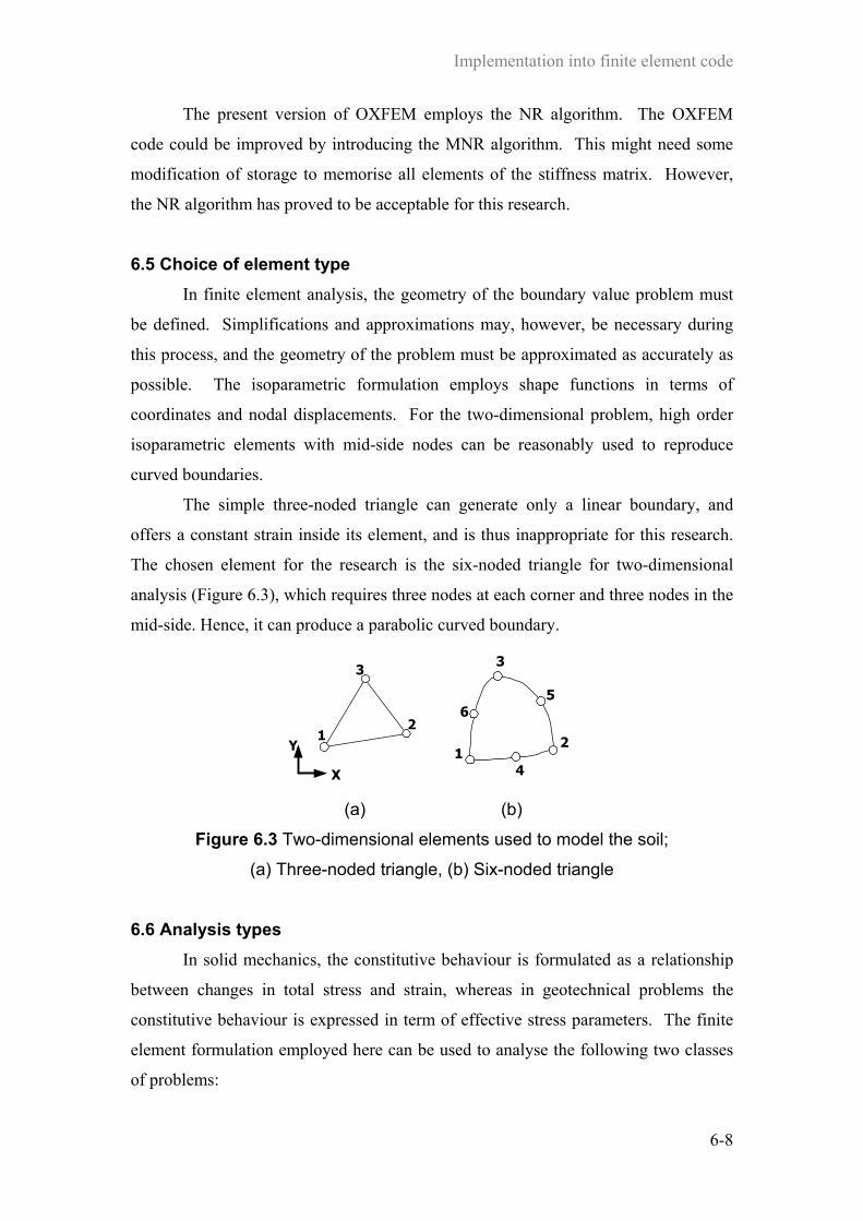
Implementation into finite element code
6-8
The present version of OXFEM employs the NR algorithm. The OXFEM
code could be improved by introducing the MNR algorithm. This might need some
modification of storage to memorise all elements of the stiffness matrix. However,
the NR algorithm has proved to be acceptable for this research.
6.5 Choice of element type In finite element analysis, the geometry of the boundary value problem must
be defined. Simplifications and approximations may, however, be necessary during
this process, and the geometry of the problem must be approximated as accurately as
possible. The isoparametric formulation employs shape functions in terms of
coordinates and nodal displacements. For the two-dimensional problem, high order
isoparametric elements with mid-side nodes can be reasonably used to reproduce
curved boundaries.
The simple three-noded triangle can generate only a linear boundary, and
offers a constant strain inside its element, and is thus inappropriate for this research.
The chosen element for the research is the six-noded triangle for two-dimensional
analysis (Figure 6.3), which requires three nodes at each corner and three nodes in the
mid-side. Hence, it can produce a parabolic curved boundary.
X
Y1
2
3
(a)
12
3
4
56
(b)
Figure 6.3 Two-dimensional elements used to model the soil;
(a) Three-noded triangle, (b) Six-noded triangle
6.6 Analysis types In solid mechanics, the constitutive behaviour is formulated as a relationship
between changes in total stress and strain, whereas in geotechnical problems the
constitutive behaviour is expressed in term of effective stress parameters. The finite
element formulation employed here can be used to analyse the following two classes
of problems:
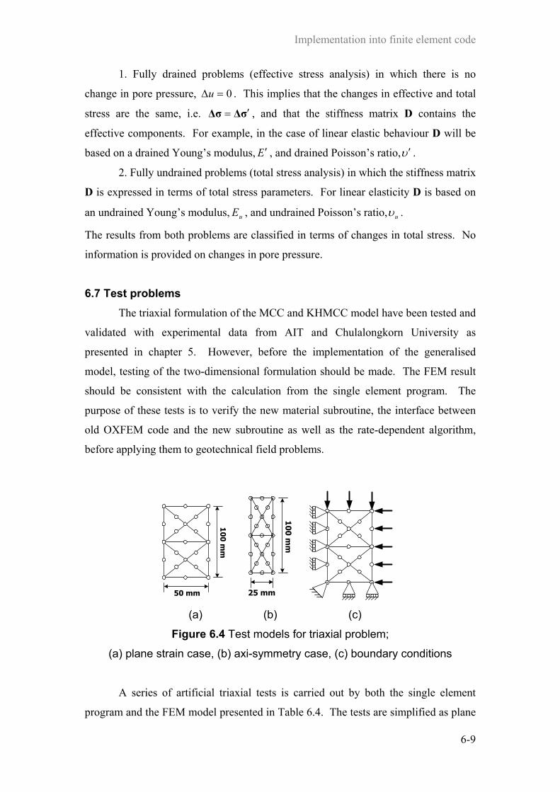
Implementation into finite element code
6-9
1. Fully drained problems (effective stress analysis) in which there is no
change in pore pressure, 0=∆u . This implies that the changes in effective and total
stress are the same, i.e. σ∆∆σ ′= , and that the stiffness matrix D contains the
effective components. For example, in the case of linear elastic behaviour D will be
based on a drained Young’s modulus, E ′ , and drained Poisson’s ratio,υ′ .
2. Fully undrained problems (total stress analysis) in which the stiffness matrix
D is expressed in terms of total stress parameters. For linear elasticity D is based on
an undrained Young’s modulus, uE , and undrained Poisson’s ratio, uυ .
The results from both problems are classified in terms of changes in total stress. No
information is provided on changes in pore pressure.
6.7 Test problems The triaxial formulation of the MCC and KHMCC model have been tested and
validated with experimental data from AIT and Chulalongkorn University as
presented in chapter 5. However, before the implementation of the generalised
model, testing of the two-dimensional formulation should be made. The FEM result
should be consistent with the calculation from the single element program. The
purpose of these tests is to verify the new material subroutine, the interface between
old OXFEM code and the new subroutine as well as the rate-dependent algorithm,
before applying them to geotechnical field problems.
50 mm
10
0 m
m
(a)
10
0 m
m
25 mm
(b)
(c)
Figure 6.4 Test models for triaxial problem;
(a) plane strain case, (b) axi-symmetry case, (c) boundary conditions
A series of artificial triaxial tests is carried out by both the single element
program and the FEM model presented in Table 6.4. The tests are simplified as plane
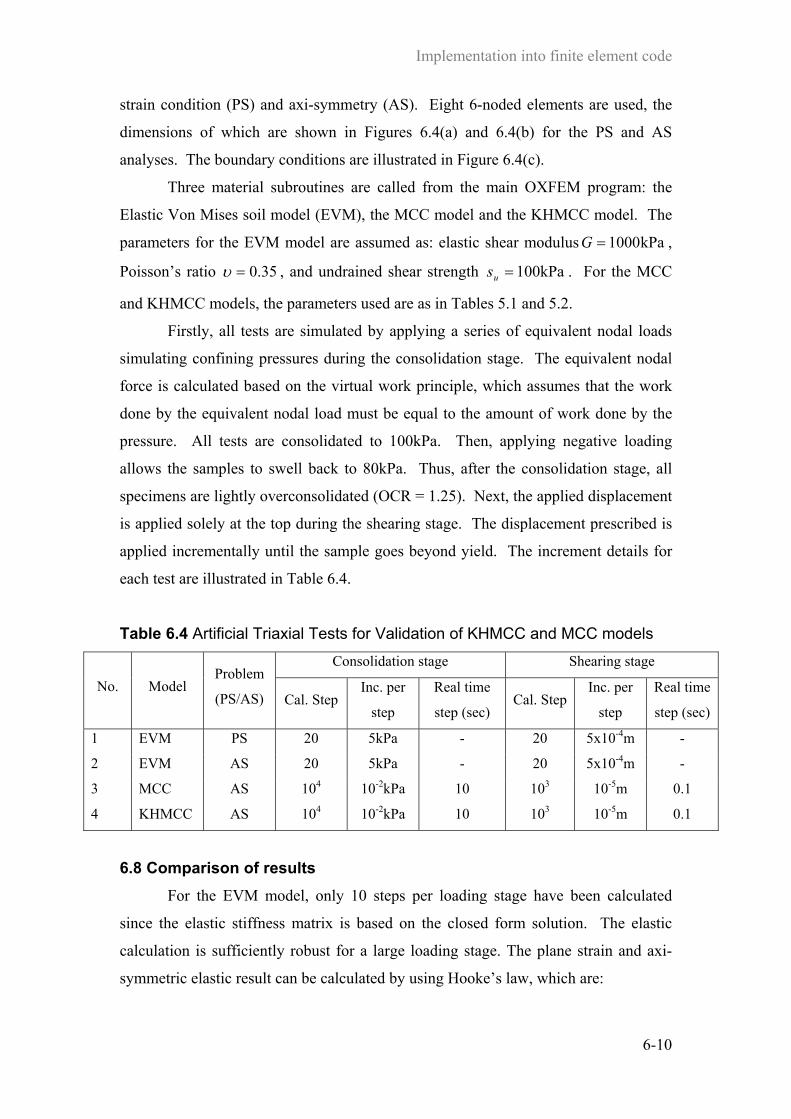
Implementation into finite element code
6-10
strain condition (PS) and axi-symmetry (AS). Eight 6-noded elements are used, the
dimensions of which are shown in Figures 6.4(a) and 6.4(b) for the PS and AS
analyses. The boundary conditions are illustrated in Figure 6.4(c).
Three material subroutines are called from the main OXFEM program: the
Elastic Von Mises soil model (EVM), the MCC model and the KHMCC model. The
parameters for the EVM model are assumed as: elastic shear modulus kPa1000=G ,
Poisson’s ratio 0.35=υ , and undrained shear strength 100kPa=us . For the MCC
and KHMCC models, the parameters used are as in Tables 5.1 and 5.2.
Firstly, all tests are simulated by applying a series of equivalent nodal loads
simulating confining pressures during the consolidation stage. The equivalent nodal
force is calculated based on the virtual work principle, which assumes that the work
done by the equivalent nodal load must be equal to the amount of work done by the
pressure. All tests are consolidated to 100kPa. Then, applying negative loading
allows the samples to swell back to 80kPa. Thus, after the consolidation stage, all
specimens are lightly overconsolidated (OCR = 1.25). Next, the applied displacement
is applied solely at the top during the shearing stage. The displacement prescribed is
applied incrementally until the sample goes beyond yield. The increment details for
each test are illustrated in Table 6.4.
Table 6.4 Artificial Triaxial Tests for Validation of KHMCC and MCC models
Consolidation stage Shearing stage
No. Model Problem
(PS/AS) Cal. Step Inc. per
step
Real time
step (sec) Cal. Step
Inc. per
step
Real time
step (sec)
1 EVM PS 20 5kPa - 20 5x10⁻⁴m -
2 EVM AS 20 5kPa - 20 5x10⁻⁴m -
3 MCC AS 104 10-2kPa 10 103 10-5m 0.1
4 KHMCC AS 104 10-2kPa 10 103 10-5m 0.1
6.8 Comparison of results For the EVM model, only 10 steps per loading stage have been calculated
since the elastic stiffness matrix is based on the closed form solution. The elastic
calculation is sufficiently robust for a large loading stage. The plane strain and axi-
symmetric elastic result can be calculated by using Hooke’s law, which are:
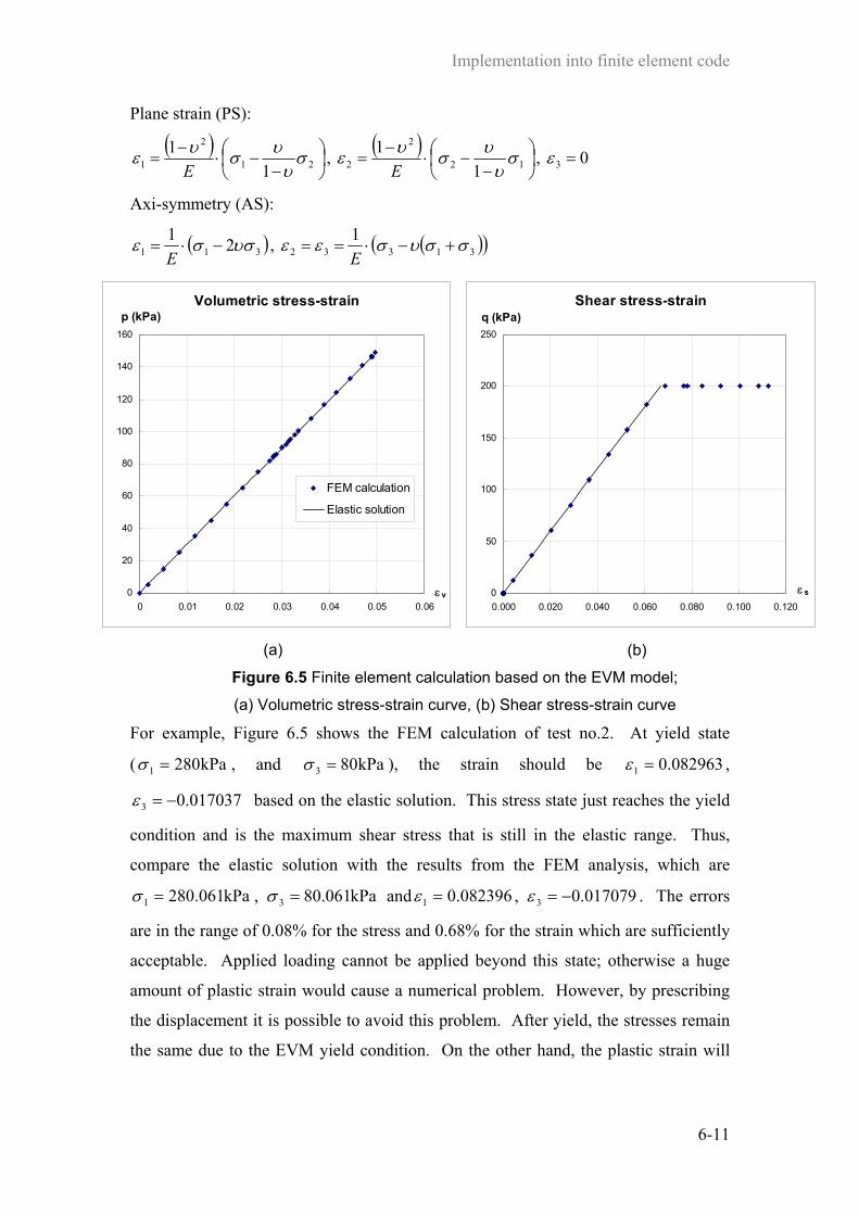
Implementation into finite element code
6-11
Plane strain (PS):
( )
−−⋅
−= 21
2
1 11 σ
υυσυε
E, ( )
−−⋅
−= 12
2
2 11 σ
υυσυε
E, 03 =ε
Axi-symmetry (AS):
( )311 21 υσσε −⋅=E
, ( )( )313321 σσυσεε +−⋅==E
Volumetric stress-strain
0
20
40
60
80
100
120
140
160
0 0.01 0.02 0.03 0.04 0.05 0.06ε v
p (kPa)
FEM calculation
Elastic solution
(a)
Shear stress-strain
0
50
100
150
200
250
0.000 0.020 0.040 0.060 0.080 0.100 0.120
ε s
q (kPa)
(b)
Figure 6.5 Finite element calculation based on the EVM model;
(a) Volumetric stress-strain curve, (b) Shear stress-strain curve
For example, Figure 6.5 shows the FEM calculation of test no.2. At yield state
( kPa2801 =σ , and kPa803 =σ ), the strain should be 082963.01 =ε ,
017037.03 −=ε based on the elastic solution. This stress state just reaches the yield
condition and is the maximum shear stress that is still in the elastic range. Thus,
compare the elastic solution with the results from the FEM analysis, which are
kPa061.2801 =σ , kPa061.803 =σ and 082396.01 =ε , 017079.03 −=ε . The errors
are in the range of 0.08% for the stress and 0.68% for the strain which are sufficiently
acceptable. Applied loading cannot be applied beyond this state; otherwise a huge
amount of plastic strain would cause a numerical problem. However, by prescribing
the displacement it is possible to avoid this problem. After yield, the stresses remain
the same due to the EVM yield condition. On the other hand, the plastic strain will

Implementation into finite element code
6-12
cause the shear strain to keep increasing. Figure 6.5 illustrates that the FEM
calculation give an accurate result for the EVM material behaviour.
Volumetric stress-strain
0
20
40
60
80
100
120
0.000 0.050 0.100 0.150 0.200ε v
p (kPa)
FEM
Single element
(a)
Stress path
0
10
20
30
40
50
60
70
0 50 100 150 200
p (kPa)
q (kPa)
(b)
Shear stress-strain
0
10
20
30
40
50
60
70
0.000 0.020 0.040 0.060 0.080 0.100
ε s
q (kPa)
(c)
Strain path
0.000
0.010
0.020
0.030
0.040
0.050
0.060
0.070
0.080
0.090
0.000 0.050 0.100 0.150 0.200ε v
ε s
(d)
Figure 6.6 Comparison of Finite element and Single element calculations based on the MCC model; (a) Volumetric stress-strain curve, (b) Stress path, (c) Shear stress-strain curve, (d) Strain path.

Implementation into finite element code
6-13
Volumetric stress-strain
0
20
40
60
80
100
120
0 0.02 0.04 0.06 0.08 0.1 0.12ε v
p (kPa)
FEM
Single element
(a)
Stress path
0
10
20
30
40
50
60
70
80
90
0 20 40 60 80 100 120
p (kPa)
q (kPa)
(b)
Shear stress-strain
0
10
20
30
40
50
60
70
80
90
0.000 0.020 0.040 0.060 0.080 0.100
ε s
q (kPa)
(c)
Strain path
0.000
0.010
0.020
0.030
0.040
0.050
0.060
0.070
0.080
0.090
0 0.02 0.04 0.06 0.08 0.1 0.12ε v
ε s
(d)
Figure 6.7 Comparison of Finite element and Single element calculations based on the KHMCC
model; (a) Volumetric stress-strain curve, (b) Stress path, (c) Shear stress-strain curve, (d) Strain
path.
For the rate-dependent calculation of the MCC and KHMCC models, the
calculation must be applied with very small increments. This is because instability of
the plastic strain will occur when the displacement is applied in large steps. There is
no closed form solution for the MCC and KHMCC models unlike the EVM model.
The comparison can be made only between the FEM and the single element
calculation. The eight elements of the FEM calculations are not significantly different
Implementation into finite element code
6-14
from the single element. The difference between two calculations is in the order of
10-4kPa (0.0001%) for the stresses and 10-7 (0.0002%) for the strains. Figures 6.6 and
6.7 show the results of tests no. 3 and 4 as compared with the single element
calculations where the line represents the single element calculation. The data points
represents the FEM results which are the average from the Gauss points of the top
element. The number of data points plotted is reduced by a factor of 100 and 1000
during the consolidation and shearing stages respectively.
6.9 Conclusion The models based on triaxial stress-strain parameters are developed from
experimental data on Bangkok clay as described in chapter 5. However,
implementation in the finite element program OXFEM is required for the generalised
models. As a result, this chapter presented the translation of models in the terms of
the generalised stress-strain parameters. This procedure needs some mathematical
processes and programming. Artificial triaxial tests are analysed to verify the
material subroutine and calculation procedure. The computer codes for rate-
dependent calculation of the MCC and KHMCC models are presented in Appendix B.
The analyses discovered that the numerical calculations are very robust in the
elastic range. The increments in the elastic range can be quite large. After the tests
reach yield state the numerical instability may occur, especially in the EVM and MCC
model. This comes from a sudden change of the behaviour from the elastic to the
plastic region. In the EVM model, the plastic range is unable to be observed by load
control because the perfectly plastic behaviour will occur after yield. The calculations
are processed using rate-independence. The analysis result is in an acceptable range
compared with the elastic solution. For the MCC and KHMCC model, the numerical
calculations are carried out using rate-dependence which is able to control the
numerical instability. By comparing between single element and FEM analyses, the
results found are that the difference is tiny. Thus, this exercise verifies that the
subroutine developed can be employed for the geotechnical field problem, which will
be discussed in the next chapter.
In addition, the analyses also found that the numerical calculation using
displacement control is slightly more robust than load control. Especially in the
shearing process where load control is not possible because a large plastic strain will
occur when the sample reaches yield. The rate-dependent algorithm with

Implementation into finite element code
6-15
displacement control will respond giving a smooth stress-strain behaviour, whereas
for load control it gives a slight non-smooth stress-strain response. This is because
the strain and strain rate are constant at any calculation step of the displacement
controlled problem.

Application to geotechnical problems
7-1
Chapter 7 Application to Geotechnical Problems
This chapter presents the application of the finite element method to the
analysis of geotechnical construction problems. This exercise applying the finite
element method is presented for the purpose of demonstrating the new constitutive
model. This is to prove that the newly developed model can be employed in
engineering practice as stated in the objectives of the research. Any further advanced
analysis such as considering the boundary effect is beyond the scope of the research
and will therefore be disregarded.
The construction problems can be categorised into two classes which are
equilibrium dominated and deformation compatibility dominated. The former relates
to the strength problem for example, shallow foundations and embankment problem.
The analysis with the advanced soil model is expected to offer an indifferent strength
prediction from the analysis with simple soil model. However, the latter deals with
the deformation problem such as earth retaining structures, and tunnelling problems.
A better deformation prediction is expected to be generated if the advanced soil model
is employed. The construction of a road embankment and tunnelling-induced
settlement are selected as two examples for this research.
7.1 Road embankment Earth embankments are built frequently for highway purposes in Thailand.
The subsoil conditions for the road embankment are mainly thick soft clay which is of
low strength and high compressibility. The design of road elevations and fill
thickness are based on the classical Terzaghi consolidation theory, which employs
compression ratio (CR) and recompression ratio (RR) as two key parameters for the
prediction of settlement and uses undrained shear strength as a strength parameter.
Embankment geometry is usually simple but, due to the weakness of the
subsoil, the embankment can be built only to a height of approximately 3m to 4m.
However, higher embankments are regularly needed in lowland area to protect from
floods. As a result, special construction methods such as reinforcement with
geotextiles and/or staged construction are necessary. In staged construction, the
embankment is constructed in stages and after each stage, a consolidated time is

Application to geotechnical problems
7-2
required for dissipation of excess pore water pressures. This process leads to a gain in
soil strength of the soft clay.
Highway No. 34 (Bangna-Trad) is one of the most economically important
highways, and problems have occurred with excessive settlement caused by the
underlying poor compressible subsoil along the route (Figure 7.1). A study of
settlement of highway no. 34 is presented by Seah (1998). The highway was initially
constructed as a two-lane highway in 1969 with design elevation of 2 to 2.8m (above
mean sea level) from chainage 0km to 55km. Ultimately, the highway was upgraded
to an eight-lane highway, and some part of roadway was on improved subsoil, using
soil cement column ground improvement.
12
CL+0.5% +3.5%
3.5 mPavement
2.75 mShoulder
Figure 7.1 Route of Highway No. 34
(Bangna-Trad Road), Seah (1998)
Figure 7.2 Typical Cross section of Highway
No. 34, Seah (1998)
7.1.1 Embankment geometry and soil conditions The construction of Bangna-Trad highway has been documented by the
Department of Highway Thailand since 1980. The typical highway cross section is
shown in Figure 7.2. However, the historical record provides only a single settlement
point at any section of road embankment. The settlement profiles are unavailable for
comparison with settlement analyses. The comparison can be only made using the
maximum settlement at the centre of the road embankment.
The original ground conditions and consolidation characteristics before
construction are represented by Seah (1998). The subsoil condition is composed of a
thick layer of very soft Bangkok clay, together with a sand layer underneath. The
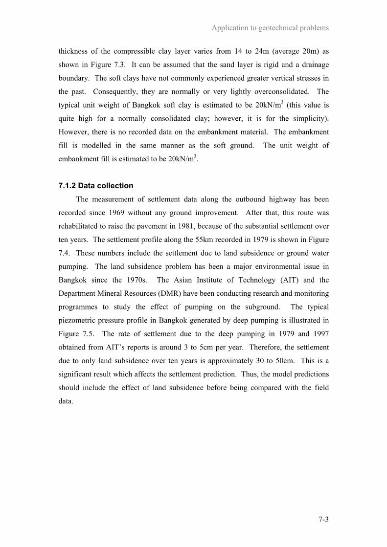
Application to geotechnical problems
7-3
thickness of the compressible clay layer varies from 14 to 24m (average 20m) as
shown in Figure 7.3. It can be assumed that the sand layer is rigid and a drainage
boundary. The soft clays have not commonly experienced greater vertical stresses in
the past. Consequently, they are normally or very lightly overconsolidated. The
typical unit weight of Bangkok soft clay is estimated to be 20kN/m3 (this value is
quite high for a normally consolidated clay; however, it is for the simplicity).
However, there is no recorded data on the embankment material. The embankment
fill is modelled in the same manner as the soft ground. The unit weight of
embankment fill is estimated to be 20kN/m3.
7.1.2 Data collection The measurement of settlement data along the outbound highway has been
recorded since 1969 without any ground improvement. After that, this route was
rehabilitated to raise the pavement in 1981, because of the substantial settlement over
ten years. The settlement profile along the 55km recorded in 1979 is shown in Figure
7.4. These numbers include the settlement due to land subsidence or ground water
pumping. The land subsidence problem has been a major environmental issue in
Bangkok since the 1970s. The Asian Institute of Technology (AIT) and the
Department Mineral Resources (DMR) have been conducting research and monitoring
programmes to study the effect of pumping on the subground. The typical
piezometric pressure profile in Bangkok generated by deep pumping is illustrated in
Figure 7.5. The rate of settlement due to the deep pumping in 1979 and 1997
obtained from AIT’s reports is around 3 to 5cm per year. Therefore, the settlement
due to only land subsidence over ten years is approximately 30 to 50cm. This is a
significant result which affects the settlement prediction. Thus, the model predictions
should include the effect of land subsidence before being compared with the field
data.
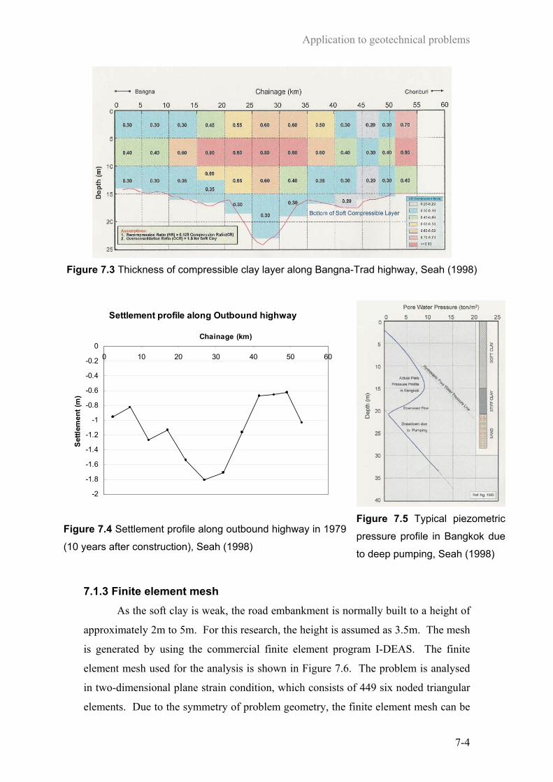
Application to geotechnical problems
7-4
Figure 7.3 Thickness of compressible clay layer along Bangna-Trad highway, Seah (1998)
Settlement profile along Outbound highway
-2
-1.8
-1.6
-1.4
-1.2
-1
-0.8
-0.6
-0.4
-0.2
00 10 20 30 40 50 60
Chainage (km)
Set
tlem
ent (
m)
Figure 7.4 Settlement profile along outbound highway in 1979
(10 years after construction), Seah (1998)
Figure 7.5 Typical piezometric
pressure profile in Bangkok due
to deep pumping, Seah (1998)
7.1.3 Finite element mesh As the soft clay is weak, the road embankment is normally built to a height of
approximately 2m to 5m. For this research, the height is assumed as 3.5m. The mesh
is generated by using the commercial finite element program I-DEAS. The finite
element mesh used for the analysis is shown in Figure 7.6. The problem is analysed
in two-dimensional plane strain condition, which consists of 449 six noded triangular
elements. Due to the symmetry of problem geometry, the finite element mesh can be

Application to geotechnical problems
7-5
reduced by half. The block of ground analysed is 20m thick and 30m wide. It is
assumed that there is a 10kPa surcharge applied on the ground surface (representing
made ground, vegetation etc.).
CL 6.25 m 7 m
3.5 m
30 m
20 m
Figure 7.6 Finite Element Mesh for Embankment of Highway No. 34
7.1.4 Constitutive models The analyses are carried out using three constitutive models; elastic Von Mises
(EVM), modified Cam-clay (MCC) and kinematic hardening modified Cam-clay
(KHMCC) model. The EVM model parameters are the Elastic shear modulus (G),
Poisson’s ratio (υ ), and Undrained shear strength (su). In the case of purely elastic
undrained analysis (EVM-1), the υ value is set to be 0.499 rather than 0.5 as the
infinite value of bulk modulus will cause a numerical problem, and su is set to be very
high (10,000kPa). The elastic-plastic undrained analysis (EVM-2) is also considered
by setting the value of su to be the undrained shear strength soft clay (10kPa). On the
other hand, for drained analysis (EVM-3), the υ value is assumed to be 0.2 which is
reasonable for soft clay and the value of su is set to be high because the purely elastic
behaviour is intended in this analysis. The MCC and KHMCC model parameters use
almost the same values that are evaluated by parametric study with the experimental
data in Table 5.1(a) and 5.1(b), the bulk and shear modulus, however, are modified to
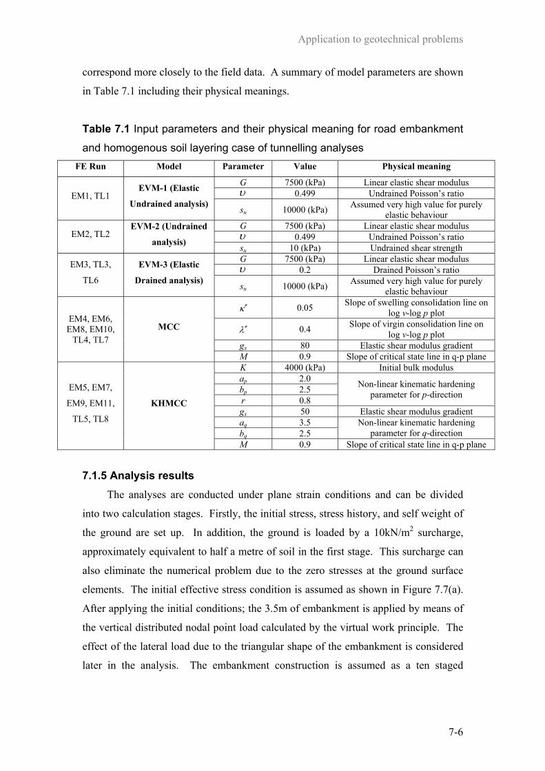
Application to geotechnical problems
7-6
correspond more closely to the field data. A summary of model parameters are shown
in Table 7.1 including their physical meanings.
Table 7.1 Input parameters and their physical meaning for road embankment
and homogenous soil layering case of tunnelling analyses FE Run Model Parameter Value Physical meaning
G 7500 (kPa) Linear elastic shear modulus υ 0.499 Undrained Poisson’s ratio EM1, TL1
EVM-1 (Elastic
Undrained analysis) su 10000 (kPa) Assumed very high value for purely elastic behaviour
G 7500 (kPa) Linear elastic shear modulus υ 0.499 Undrained Poisson’s ratio EM2, TL2
EVM-2 (Undrained
analysis) su 10 (kPa) Undrained shear strength G 7500 (kPa) Linear elastic shear modulus υ 0.2 Drained Poisson’s ratio EM3, TL3,
TL6
EVM-3 (Elastic
Drained analysis) su 10000 (kPa) Assumed very high value for purely elastic behaviour
κ∗ 0.05 Slope of swelling consolidation line on log v-log p plot
λ∗ 0.4 Slope of virgin consolidation line on log v-log p plot
gx 80 Elastic shear modulus gradient
EM4, EM6, EM8, EM10,
TL4, TL7 MCC
M 0.9 Slope of critical state line in q-p plane K 4000 (kPa) Initial bulk modulus ap 2.0 bp 2.5 r 0.8
Non-linear kinematic hardening parameter for p-direction
gx 50 Elastic shear modulus gradient aq 3.5 bq 2.5
Non-linear kinematic hardening parameter for q-direction
EM5, EM7,
EM9, EM11,
TL5, TL8
KHMCC
M 0.9 Slope of critical state line in q-p plane 7.1.5 Analysis results
The analyses are conducted under plane strain conditions and can be divided
into two calculation stages. Firstly, the initial stress, stress history, and self weight of
the ground are set up. In addition, the ground is loaded by a 10kN/m2 surcharge,
approximately equivalent to half a metre of soil in the first stage. This surcharge can
also eliminate the numerical problem due to the zero stresses at the ground surface
elements. The initial effective stress condition is assumed as shown in Figure 7.7(a).
After applying the initial conditions; the 3.5m of embankment is applied by means of
the vertical distributed nodal point load calculated by the virtual work principle. The
effect of the lateral load due to the triangular shape of the embankment is considered
later in the analysis. The embankment construction is assumed as a ten staged

Application to geotechnical problems
7-7
construction is which ten steps of calculation is applied for the loading stage.
Descriptions of the road embankment analyses are summarised in Table 7.2.
Normally consolidated soil
-30
-25
-20
-15
-10
-5
00 100 200 300
vertical stress (kPa)
dept
h (m
)
(a)
Overconsolidated soil
-30
-25
-20
-15
-10
-5
00 100 200 300
vertical stress history (kPa)
dept
h (m
)
(b) Figure 7.7 Distribution of vertical stress with depth; (a) in-situ vertical stress for
overconsolidated soil and normally consolidated soil. (b) maximum past vertical stress
for overconsolidated soil
Table 7.2 Description of finite element analyses of road embankment
FE Run Model Analysis type K0 Surface
crust
Horizontal
load
Maximum
settlement (cm)
EM1 EVM-1 Undrained 1 - - 2.06
EM2 EVM-2 Undrained 1 - - 10.83
EM3 EVM-3 Drained 1 - - 6.10
EM4 MCC Drained 1 - - 32.77
EM5 KHMCC Drained 1 - - 20.81
EM6 MCC Drained 0.7 - - 42.84
EM7 KHMCC Drained 0.7 - - 24.19
EM8 MCC Drained 1 Yes - 32.14
EM9 KHMCC Drained 1 Yes - 20.43
EM10 MCC Drained 1 - Yes 29.74
EM11 KHMCC Drained 1 - Yes 19.67
The ground settlement profiles for analyses EM1 to EM5 are shown in Figure
7.8. The analyses EM1 and EM3 offer only purely elastic stiffness when the soil
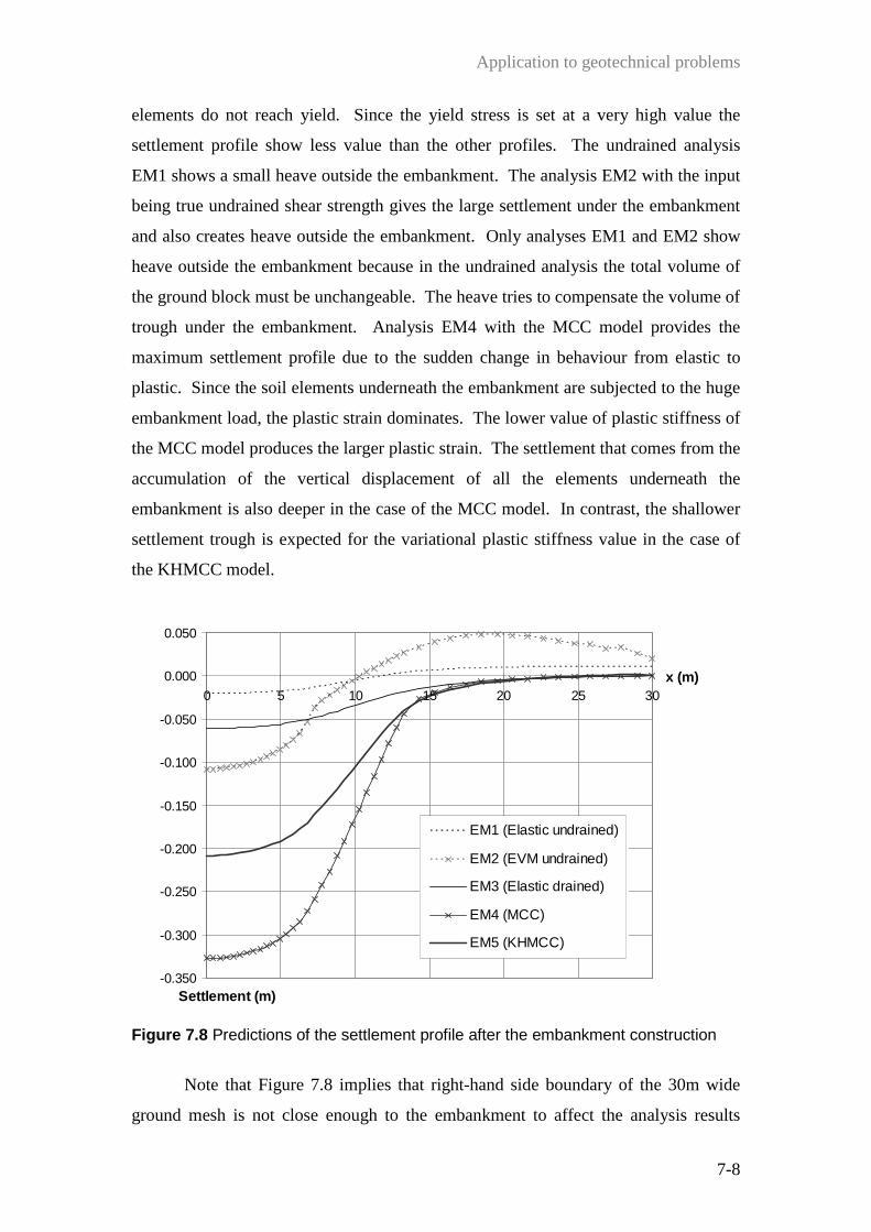
Application to geotechnical problems
7-8
elements do not reach yield. Since the yield stress is set at a very high value the
settlement profile show less value than the other profiles. The undrained analysis
EM1 shows a small heave outside the embankment. The analysis EM2 with the input
being true undrained shear strength gives the large settlement under the embankment
and also creates heave outside the embankment. Only analyses EM1 and EM2 show
heave outside the embankment because in the undrained analysis the total volume of
the ground block must be unchangeable. The heave tries to compensate the volume of
trough under the embankment. Analysis EM4 with the MCC model provides the
maximum settlement profile due to the sudden change in behaviour from elastic to
plastic. Since the soil elements underneath the embankment are subjected to the huge
embankment load, the plastic strain dominates. The lower value of plastic stiffness of
the MCC model produces the larger plastic strain. The settlement that comes from the
accumulation of the vertical displacement of all the elements underneath the
embankment is also deeper in the case of the MCC model. In contrast, the shallower
settlement trough is expected for the variational plastic stiffness value in the case of
the KHMCC model.
-0.350
-0.300
-0.250
-0.200
-0.150
-0.100
-0.050
0.000
0.050
0 5 10 15 20 25 30x (m)
Settlement (m)
EM1 (Elastic undrained)
EM2 (EVM undrained)
EM3 (Elastic drained)
EM4 (MCC)
EM5 (KHMCC)
Figure 7.8 Predictions of the settlement profile after the embankment construction
Note that Figure 7.8 implies that right-hand side boundary of the 30m wide
ground mesh is not close enough to the embankment to affect the analysis results

Application to geotechnical problems
7-9
except for the analysis EM2 which uses a very low input value of undrained shear
strength (10kN/m2).
The stresses are controlled by the initial ground conditions and applied nodal
loads. Therefore, they do not vary significantly in each case from analyses EM1 to
EM5. The typical horizontal ( hσ ′ ) and vertical ( vσ ′ ) stress contours selected from
analysis EM4 with the MCC model are in the ranges of -200 to 5kPa and -220 to
-25kPa respectively as shown in Figures 7.9(a) and (b), where the negative sign
convention indicates compression. The strains are controlled by the constitutive
model and the analysis condition (i.e. drained or undrained). The horizontal ( hε ) and
vertical ( vε ) strain contours of analysis EM4 are in the range of -0.02 to 0.02 and
-0.06 to 0.01 respectively as shown in Figures 7.9(c) and (d). The patterns of strain
distribution for analyses EM4 and EM5 respectively, using the MCC and KHMCC
models, are similar except for the contour range of -0.02 to 0.01 for the KHMCC
model as shown in Figure 7.10(d). This is because the analysis EM4 shows a deeper
settlement than EM5 and hence higher plastic strains are expected for the lower
plastic stiffness. The analyses EM1 and EM3 with purely elastic responses exhibit a
unique pattern of strain distribution. The maximum compressive strain of analysis
EM3 however is two times larger than analysis EM1 due to the difference between
undrained and drained analysis as shown in Figures 7.10(a) and (c). For the
undrained analysis EM2 with low su, the strain distribution takes no identifiable form:
the plot is scattered, however it can be represented as a slip line under the
embankment (see Figures 7.10 (b) and 7.11(d)). This is because the stress amplitude
of almost all elements reaches yield as shown in Figure 7.11(b). The stress amplitude
( ( ) 2minmax σσ ′−′ ) and strain amplitude ( ( ) 2minmax εε − ) values can imply the state of
stress and strain in the yield condition. Figures 7.11(a) and (c) show the typical stress
and strain amplitude contours of the embankment, which are selected from analysis
EM4.
Figure 7.12(a) shows the nodal force vector for all nodal points in the problem.
The nodal force is determined by the boundary conditions and ground conditions.
The force on the surface boundary corresponds to the applied surcharge load from the
embankment. Both sides of the boundaries correspond to the roller support condition
(fixed horizontal movement) and the nodal forces distribute in a triangular pattern
which corresponds to the horizontal stress. The nodal forces at the bottom boundary

Application to geotechnical problems
7-10
correspond to the total reaction force due to the gravity load and the applied surcharge
embankment. The nodal displacement vectors for all nodal points of analyses EM4,
EM2 and EM3 are shown in Figures 7.12(b), (c) and (d) respectively. For undrained
analysis EM2 (Figure 7.12(c)), all displacement vectors move outward due to the
embankment surcharge as expected. On the other hand, all displacements for drained
analyses EM4 and EM3 (Figures 7.12(b) and (d)) surprisingly move inward due to the
embankment surcharge. There are still no obvious evidence that shows this
phenomenon occurring for the drained case. The critical process of embankments on
soft clay is during the construction, which must be analysed as undrained or partially
drained, rather than drained condition. Few data exist for drained settlement of
embankment on soft clays.
Analyses EM6 and EM7 consider the effect of effective stress ratio (K0). In
analyses EM1 to EM5, an assumption of 10 =K is made. However, the actual ground
does not have isotropic stress conditions. Several experimental data from AIT such as
Kim (1991) and Khan (1999) conclude that the value of K0 is less than unity and
around 0.6 to 0.8. Thus, in analysis EM6 and EM7, 7.00 =K is assumed.
In addition, the most critical issue for embankments on soft clay is the strength
of the clay. The top soil layer normally has a high strength and OCR value due to its
stress history. The crust can have a marked effect on the behaviour of an
embankment. To illustrate the effect of the surface crust, analyses EM8 and EM9
with a distribution of OCR as shown in Figure 7.7 have been performed. The
comparisons of the results after considering the effect of K0 and the effect of the
surface crust are shown in Figure 7.13.
The effect of surface crust makes the settlement profile slightly shallower as
shown in Figure 7.13. This stress history effect can be modelled by specifying the
maximum past stress (see input to OXFEM in appendix A). In contrast, the effect of
K0 makes the settlement profile deeper, when reducing the K0 value from 1.00 to 0.70.

(a
)
(b)
(c
)
(d)
Fig
7.9
The
stre
ss a
nd s
train
con
tour
s of
the
anal
ysis
EM
4 w
ith M
CC
mod
el
(a) h
oriz
onta
l stre
ss c
onto
ur (
hσ′ ,
kP
a); (
b) v
ertic
al s
tress
con
tour
(v
σ′ ,
kP
a);(c
) hor
izon
tal s
train
con
tour
(hε, -
); (d
) ver
tical
stra
in c
onto
ur (
vε, -
)
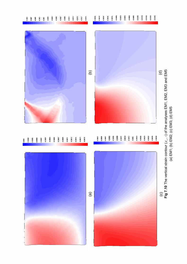
(a
)
(b)
(c
)
(d)
Fig
7.10
The
ver
tical
stra
in c
onto
ur (
vε, -
) of t
he a
naly
ses
EM
1, E
M2,
EM
3 an
d E
M5
(a) E
M1;
(b) E
M2;
(c) E
M3;
(d) E
M5

(a
)
(b)
(c
)
(d)
Fig
7.11
The
stre
ss a
nd s
train
am
plitu
de c
onto
ur o
f the
ana
lyse
s E
M4
and
EM
2 (a
) and
(c) a
re th
e st
ress
am
plitu
de o
f EM
4 an
d E
M2
resp
ectiv
ely,
kP
a; (b
) and
(d) a
re th
e st
rain
am
plitu
de o
f EM
4 an
d E
M2
resp
ectiv
ely

(a
)
(b)
(c
)
(d)
Fig
7.12
The
nod
al fo
rce
and
disp
lace
men
t vec
tor o
f the
ana
lyse
s E
M2,
EM
3, E
M4
(a) T
he n
odal
forc
e ve
ctor
of E
M4;
(b),
(c) a
nd (d
) are
the
noda
l dis
plac
emen
t vec
tor o
f EM
4, E
M2
and
EM
3 re
spec
tivel
y

Application to geotechnical problems
7-15
-0.450
-0.400
-0.350
-0.300
-0.250
-0.200
-0.150
-0.100
-0.050
0.0000 5 10 15 20 25 30
x (m)
Settlement (m)
EM4 (MCC)
EM5 (KHMCC)
EM6 (MCC-Ko reduction)
EM7 (KHMCC-Ko reduction)
EM8 (MCC-crust)
EM9 (KHMCC-crust)
Figure 7.13 Predictions of the settlement profile with effect of the surface crust and
stress ratio (K0)
The replacement of the soil embankment by a vertical nodal load can accurately
approximate a uniform wide embankment. The triangular embankment should be
replaced by vertical and horizontal distributed nodal load. However, the horizontal
load is relatively small compared with the whole size of the embankment. The
approximations of embankment nodal loads in the analyses are displayed in Figures
7.14(a) and (b). The evaluation of horizontal loads starts from the definition of active
pressure: vaa K σσ = and then calculates the active force: hKP vaa σ21= . The
summation of all horizontal nodal loads must be equal hKP vaa σ21= and this
amount has to triangularly distribute along the distance L as shown in Figure 7.14(c).
The analysis results of EM10 and EM11 considering the effect of horizontal nodal
load are presented in Figure 7.15. As the displacement vector moves inward, the
lateral load on the opposite side will cancel the displacement vector. Thus, the lateral
load makes the trough slightly shallower and wider.

Application to geotechnical problems
7-16
(a)
(b)
Kaσv
1/2Kaσvh
Kaσv(h/L)
1/2Kaσv(h/L)L
L
h
(c)
Figure 7.14 Equivalent nodal force of soil embankment load
(a) Vertical nodal load; (b) Effect of lateral nodal load; (c) Estimation of lateral nodal load
-0.350
-0.300
-0.250
-0.200
-0.150
-0.100
-0.050
0.0000 5 10 15 20 25 30
x (m)
Settlement (m)
EM4 (MCC)
EM5 (KHMCC)
EM10 (MCC-lateral load)
EM11 (KHMCC-lateral load)
Figure 7.15 Predictions of the settlement profile with effect of lateral nodal load
Figure 7.16(a) presents the effect of the horizontal shear nodal force under the
triangular embankment. The horizontal shear force tries to drag the horizontal
displacement in the outward direction from the embankment. This leads to the
reduction of the vertical settlement and can be illustrated by the displacement vector
as shown in Figure 7.16(b).
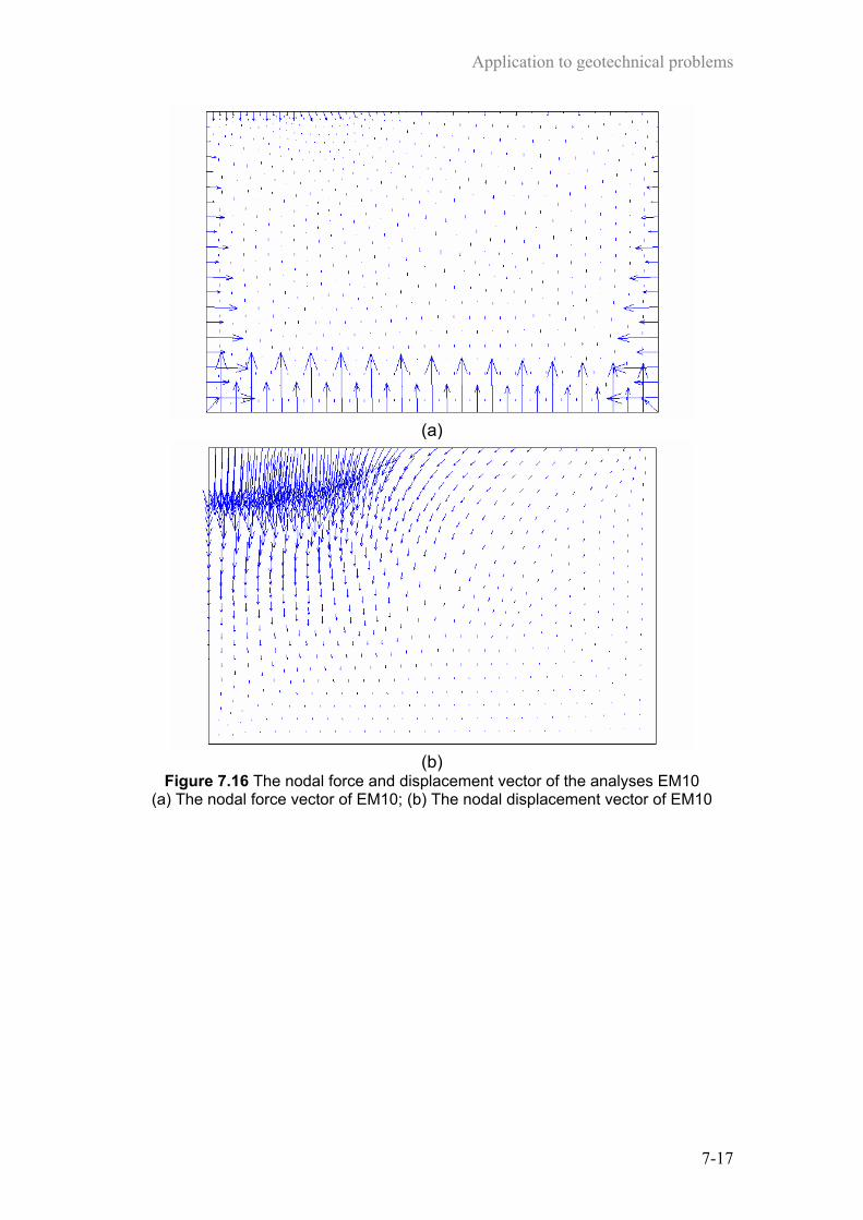
Application to geotechnical problems
7-17
(a)
(b)
Figure 7.16 The nodal force and displacement vector of the analyses EM10 (a) The nodal force vector of EM10; (b) The nodal displacement vector of EM10

Application to geotechnical problems
7-18
7.2 Tunnelling The analysis of tunnels using the finite element method is commonly used in
practical design. In the conventional designs, the load characteristics are determined
by a technique which is mostly elastic and movements by a technique which is
principally empirical. Nevertheless, there two techniques are not linked. In order to
progress the understanding of design methods for building interaction with tunnelling-
induced settlements, much research on tunnelling has been conducted such as Lee and
Rowe (1989) and Addenbrooke et al. (1997).
The Civil Engineering Research Group at Oxford University has also been
undertaken the tunnelling research since 1993. A number of two-dimensional finite
element analyses of a building and ground were carried out by Liu (1997). A nested
yield surface model offering a variation of stiffness was implemented in the finite
element for this study. The other factors affecting the tunnelling-induced settlement
such as percentage of volume loss, in-situ stress ratio ( vhK σσ= ), density of soil,
choice of external fixity to lining, and modification of parameters for the nested yield
surface model were further studied by Bloodworth (2002).
For three-dimensional numerical modelling, the tunnelling processes for
assessment of damage to buildings were analysed by Augarde (1997). Then, three-
dimensional finite element modelling of lined tunnelling problems was performed by
Augarde and Burd (2001). The choice of structural liner was studied using two
different elements to model the tunnel lining.
As stated in the introduction, this tunnelling problem is used to demonstrate
the new constitutive model. The analysis procedure here is performed by following
the standard approach from previous research by Bloodworth (2002).
7.2.1 Empirical prediction of tunnelling-induced settlement An empirical formulation for predicting the short-term transverse settlement
trough could be approximated by a normal distribution or Gaussian curve. The
equation for the assumed trough shape is:
−⋅= 2
2
max 2exp
ixSS (7.1)
where maxS is the maximum settlement above the tunnel axis and x is the transverse
distance from the tunnel axis. The width of the settlement trough is defined by the
Application to geotechnical problems
7-19
parameter i (distance from the axis to the inflexion point of Gaussian curve) which
varies according to the depth of the tunnel and the nature of the ground. O’Reilly and
New (1991) expressed the trough width parameter in the form of zKi ⋅= , where z is
the depth of the tunnel axis below ground level. For cohesive soil K is normally in the
range of 0.4 to 0.5.
Another parameter to control the amount of settlement is the volume loss (VL).
The volume loss can be estimated by using the volume of the settlement trough (Vs) or
the displacement of tunnel lining after excavation. For the undrained analysis, the
volume losses calculated from both definitions must be the same. Integrating
equation 7.1 to evaluate the volume of the trough, the expression
becomes max2 iSVs ⋅= π .
7.2.2 Model ground conditions and input soil properties The numerical research and design on tunnelling, especially in soft clay are
widely studied in Thailand due to the fact that a large tunnel project for a subway
system is currently under construction by the Metropolitan Rapid Transit Authority
(MRTA). The typical geological condition of MRTA project is displayed in Figure
7.17(a). The tunnel mainly involves excavation in stiff to very stiff clay using an
Earth Pressure Balance shield (EPB). The dimension of the shield machine is 6.45m
in diameter and 6m in length and the cutting speed can reach to 100mm/min.
Lin et al. (2002) has been studied three-dimensional deformation due to use of
EPB shield tunnelling in Bangkok subsoil. Additionally, this analysis presents the
field instrumented data of the MRT Blue Line Subway tunnel (RE-5T-06). The
observations of settlement trough at various depths for various stages of tunnel
advancement are recorded. The plane strain condition can be assumed when the
tunnel goes far enough through the observed station. The tunnel lies on the dense
sand layer, which is assumed to be rigid and a drainage boundary for analysis as
shown in Figure 7.17(b).
The two-dimensional plane strain condition is assumed for the analysis of
MRTA project, as shown in Figure 7.17(b). In general, the soils have much stiffer
behaviour when further soils have been deposited on the top. The first 2.5m is made
ground, and can be assumed as a crust. However, this crust has not induced much
effect on the settlement trough, so the high OCR value of the top soil layer can be

Application to geotechnical problems
7-20
disregarded. Therefore, the 14m top of Soft Clay to Medium Clay can be modelled as
normally or very lightly overconsolidated. Next, the second layer of Stiff Clay to
Very Stiff Clay can be assumed for the rest of ground between 14m to 25m. The
typical unit weight of Bangkok soft clay is still estimated to be 20kN/m3 for all layers
and the initial stress and stress history can also be assumed as in Figure 7.12(a).
The typical construction design and analysis in Bangkok assumes the first
dense sand layer as a rigid layer. This is due to the fact that the engineering properties
such as compressibility, strength and drainage are distinctively different from the
adjacent clay layers. The analysis here therefore approximates the first dense sand as
a rigid foundation as shown in Figure 7.17(b).
Made ground
Soft Clay
Medium Clay
Stiff Clay
Very stiff Clay
1st Dense sand
Very stiff Clay
0 m
2.5 m
12.8 m
14 m
18.7 m
25 m26.7 m
33.9 m
Elev
atio
n (m
) 23 m
(a)
Soft to Medium Clay
Stiff to Very stiff Clay
Assumed rigid foundation
0 m
2.5 m
12.8 m
14 m
18.7 m
25 m
23 m
Elev
atio
n (m
)
(b)
Figure 7.17 (a) Typical geological condition of Metropolitan Rapid Transit Authority (MRTA) project at
Bangkok Thailand; (b) Assumed ground condition for analysis of MRTA project, Lin et. al (2002)
7.2.3 Model of lining In order to model the concrete lining for the MRTA project, there are several
alternatives to model the lining; both in terms of the liner structures and constitutive
laws. In Augarde and Burd (2001), a comparison between the linings modelled by
shell elements and continuum elements was made. The paper reported that the liner

Application to geotechnical problems
7-21
behaviour depends on the stiffness ratio between soil and liner ( linersoil EE ). For
small values of this stiffness ratio, the liner behaves as a stiff tube and displacements
are small. For the larger values of the stiffness ratio, the liner response is more
flexible and displacements are larger. In addition, the paper noted that the shell
element formulations do not exhibit flexural behaviour that is excessively stiff (called
over-stiff).
In this research, the liner structural elements use 16 six-noded continuum
elements with an aspect ratio (thickness/radius) of 0.1. The elastic Von Mises (EVM)
constitutive law is selected for modelling of concrete lining. The concrete properties
were assumed as follows: Young’s modulus E = 24GPa, Poisson’s ratio υ = 0.2, and
compressive strength cf ′ = 30MPa. These properties can be converted to the EVM’s
parameters where shear modulus G = 10GPa, and su =15MPa. The liner behaves as a
flexible liner according to Augarde and Burd (2001). This is because the stiffness
ratio between soil and liner ( linersoil EE ) is around 0.3 to 0.5.
7.2.4 Finite element mesh
50 m
CL
10 m
14 m
5 m
6 m
(a)

Application to geotechnical problems
7-22
Layer of continuumlining elements
0.1RR
(b)
Figure 7.18 (a) Finite element mesh
for MRTA project; (b) Tunnel lining
details
The mesh for tunnel problem is generated by using the commercial finite
element program I-DEAS. In this study, the tunnel problem is simulated as a two-
dimensional plane strain problem with 1105 six-noded triangular elements. By taking
advantage of the symmetry of the problem one can reduce the amount of calculation
by half. The boundary conditions are assumed as roller supports for the side and fixed
supports for the bottom. The finite element mesh for the MRTA project is presented
in Figure 7.18(a). Moreover, the detail of tunnel lining mesh is shown in Figure
7.18(b).
7.2.5 Choice of constitutive model The analyses of the tunnel problem have been carried out using several
advanced soil models. The models are generally claimed their own advantages for
prediction of the settlement trough due to tunnel excavation. The simplest linear
elasticity model is still used to analyses the tunnel problem; however, some
modifications have been added such as anisotropic or nonlinear elasticity,
Addenbrooke et al. (1997). The results of elastic analyses indicate that the settlement
profile is too shallow and too wide when being compared with field data. Linear
isotropic elasticity predicts a profile of the wrong shape. Linear anisotropic elasticity
offers a better shape of the settlement profiles. However, it does not considerably
improve the prediction. Nonlinear elasticity provides a transition of stiffness;
however, the unloading stiffness is still based on the exact loading curve which is in
the wrong direction. To provide this, the plasticity models are recommended.

Application to geotechnical problems
7-23
For plasticity models, several elastic perfectly plastic soil models have been
proposed. For instance Von Mises, Mohr-Coulomb, Drucker-Prager (1952) and
Matsuoka-Nakai (1974). However, the critical state model known as the MCC model
is also used. These models offer the elastic behavior solely within the yield surface.
Thus, using them to predict the settlement may not be correct, especially for
overconsolidated soils. Several advanced models such as the Bubble model, (Al-
Tabbaa and Wood, 1987) and MIT-E3 model, (Whittle, 1993) are still difficult to use
according to the complication of their expressions, which may not be implemented in
numerical code easily.
The Three-surface kinematic hardening model, (Atkinson and Stallebrass, 1991)
has been employed in the CRISP finite element program to demonstrate the effect of
recent stress history on a two-dimensional tunnel problem, (Stallebrass, Jovicic and
Taylor, 1994). The study illustrates that the surface settlement profiles were
significantly affected by the recent stress history. This evidence implies that the
multiple yield surfaces model, which explains the immediate stress history, is able to
improve the numerical prediction of ground movements around a tunnel. Thus, the
KHMCC model with multiple kinematic hardening yield surfaces should exhibit the
effects of immediate stress history on tunnelling-induced settlement.
7.2.6 Analysis result The analyses are done in plane strain conditions for different soil models. The
analyses are divided into three calculation stages. At first, initial stress, stress history,
and self-weight of the ground are set up. In addition, the ground is loaded by a
10kN/m2 surcharge, which is approximately equivalent to 0.5m of soil. Next, the
tunnel elements are removed and the lining elements are inserted. Finally, the internal
pressure is incrementally applied, divided into 100 steps of loading. The internal
pressure, which controls the volume loss, is calculated and replaced by the nodal
force. The volume loss can be calculated from either the surface trough or the
displacement of the lining. In general, the volume loss should be controlled in the
range of 1 or 2% of tunnel volume.
All descriptions of the two-dimensional plane strain finite element analyses are
summarised in Table 7.3. Analyses TL1 to TL5 for homogeneous soil have been
performed using three models (i.e. EVM, MCC and KHMCC). Three different sets of
EVM can be categorised, i.e. EVM-1 for elastic undrained analysis, EVM-2 for elastic
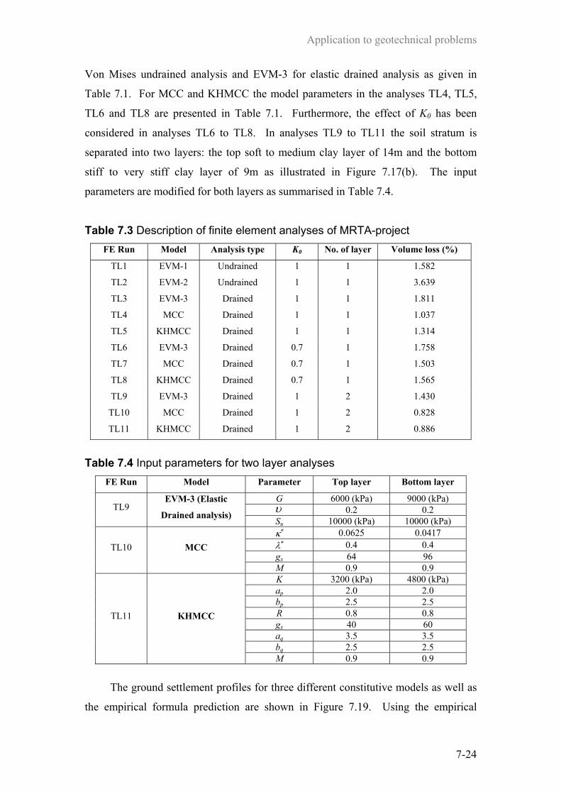
Application to geotechnical problems
7-24
Von Mises undrained analysis and EVM-3 for elastic drained analysis as given in
Table 7.1. For MCC and KHMCC the model parameters in the analyses TL4, TL5,
TL6 and TL8 are presented in Table 7.1. Furthermore, the effect of K0 has been
considered in analyses TL6 to TL8. In analyses TL9 to TL11 the soil stratum is
separated into two layers: the top soft to medium clay layer of 14m and the bottom
stiff to very stiff clay layer of 9m as illustrated in Figure 7.17(b). The input
parameters are modified for both layers as summarised in Table 7.4.
Table 7.3 Description of finite element analyses of MRTA-project FE Run Model Analysis type K0 No. of layer Volume loss (%)
TL1 EVM-1 Undrained 1 1 1.582
TL2 EVM-2 Undrained 1 1 3.639
TL3 EVM-3 Drained 1 1 1.811
TL4 MCC Drained 1 1 1.037
TL5 KHMCC Drained 1 1 1.314
TL6 EVM-3 Drained 0.7 1 1.758
TL7 MCC Drained 0.7 1 1.503
TL8 KHMCC Drained 0.7 1 1.565
TL9 EVM-3 Drained 1 2 1.430
TL10 MCC Drained 1 2 0.828
TL11 KHMCC Drained 1 2 0.886
Table 7.4 Input parameters for two layer analyses FE Run Model Parameter Top layer Bottom layer
G 6000 (kPa) 9000 (kPa) υ 0.2 0.2 TL9
EVM-3 (Elastic
Drained analysis) Su 10000 (kPa) 10000 (kPa) κ∗ 0.0625 0.0417 λ∗ 0.4 0.4 gx 64 96
TL10 MCC
M 0.9 0.9 K 3200 (kPa) 4800 (kPa) ap 2.0 2.0 bp 2.5 2.5 R 0.8 0.8 gx 40 60 aq 3.5 3.5 bq 2.5 2.5
TL11 KHMCC
M 0.9 0.9
The ground settlement profiles for three different constitutive models as well as
the empirical formula prediction are shown in Figure 7.19. Using the empirical

Application to geotechnical problems
7-25
formula in equation 7.1 to predict a settlement trough; assuming the parameter
zi ⋅= 5.0 , the volume loss can be calculated as 1.295%. All predictions are
consistent with the observed data from MRTA project (Lin et. al, 2002) except TL2.
All calculations are done without consolidation analysis (i.e. fully undrained analysis
or fully drained analysis), the undrained analyses TL1 and TL2 only show the total
stress result. In analysis TL1 undrained conditions are assumed with very high
undrained shear strength, thus the settlement trough is much shallower than the result
from TL2. Analysis TL2 gives the deepest trough as the analysis is done with the
actual undrained shear strength, which is at a lower strength than in other analyses.
On the other hand, the drained analyses TL3, TL4 and TL5 show effective stress
behaviour. All predicted troughs are consistent with the empirical formula and the
field data as shown in Figure 7.19(a). However, this cannot confirm the accuracy of
the model behaviour since only one set of field data is used as a comparison. Analysis
TL3 with the EVM model illustrates a slightly deeper and wider trough than the other
predictions do. Analysis TL4 with the MCC model shows a small heave at the far end
of the boundary. This may be due to the flow direction of strain vectors which move
inward to the tunnel for the elements near the tunnel and move upward for the ground
surface elements at the farther side. Analysis TL5 with the KHMCC model gives a
shallower and wider trough shape than TL4. These predictions can be improved by
modifying the ground, such as stress history or soil layering.
The analyses TL6, TL7 and TL8 with a reduction of K0 from 1.00 to 0.70 show
a deeper and narrower trough than TL3, TL4 and TL5. This may be due to the
direction of major principal stress which is in the vertical direction when K0 less than
1.00, and this results in the major principal strain also approximately in the vertical
direction. Thus, the vertical displacement is expected to be higher than in analysis
with K0 equal to 1.00. This was also found by Addenbrooke et. al (1997), in which
analyses were carried out reducing of K0 from 1.50 to 0.50 around the tunnel zone.
The settlement troughs of TL6, TL7 and TL8 are illustrated in Figure 7.19(b), and
compared with TL3, TL4 and TL5.
The analyses improved by splitting the ground into two regions as shown in
Figure 7.19(b) as presented in analyses TL9, TL10 and TL11. In these analyses, the
stiffness values of the top and bottom layer can be adjusted until satisfied. For the
consistency of all model comparisons, however, the stiffness parameters are modified
from the analyses TL3, TL4 and TL5 by a factor of 0.8 and 1.2 for the top and bottom
Application to geotechnical problems
7-26
soil layers respectively as illustrated in Figure 7.20. The analyses results of TL9,
TL10 and TL11 are displayed in Figure 7.19(c), and are comparable with TL3, TL4
and TL5.
The horizontal ( hσ ′ ) and vertical ( vσ ′ ) stress contours for analysis TL4 with the
MCC model are in the range of -390 to 0kPa and -490 to -10kPa respectively as
presented in Figures 7.21(a) and (b). This case is presented since the stresses are
similar for each of analyses TL1 to TL11. The horizontal stress increases at the
crown and reduces at the springline of the tunnel as shown in the contour plot in
Figure 7.21(a). On the other hand, the vertical stress decreases at the crown and
becomes greater at the springline of the tunnel. The strains, however, depend
principally on the choice of the constitutive model and the analysis conditions (i.e.
drained or undrained analysis). The horizontal ( hε ) and vertical ( vε ) strain contours
from analysis TL4 are in the range of -0.005 to 0.007 and -0.006 to 0.005 respectively
shown in Figures 7.21(c) and (d). Figure 7.22 presents four examples of vertical
strain contours from analyses TL2, TL5, TL7 and TL10. The undrained analysis TL2
with the low input shear strength as shown in Figure 7.22(a) indicates that the vertical
strains are tensile for all elements above the tunnel. This causes a deep settlement
trough. The result of analysis TL5 (Figure 7.22(b)) with the KHMCC model shows a
smoother transition of vertical strain than for the MCC model. The reduction of K0
leads to an increase in the vertical strain as shown in Figure 7.22(c). Figure 7.22(d)
shows the discontinuity of the stress contour at the boundary between soft and stiff
clay due to the sudden change of stiffness from a soft to a stiff layer.
The stress and strain amplitude contours from analyses TL4 and TL2 are
presented in Figure 7.23. Figures 7.23(b) and 7.23(d) illustrate the state of soil
elements around the tunnel reaching the yield state (i.e. ( ) Gsu=− minmax εε ). This
comes from the fact that the soil elements near the tunnel reach the yield state first
and then the stress will gradually transfer to the adjacent elements. Figures 7.23(a)
and 7.23(c) exhibit the typical stress and strain amplitude contour of analysis TL4
since they are moderately similar in each analysis except in some details such as
magnitude of contours.

Application to geotechnical problems
7-27
Settlement Trough
-20
-18
-16
-14
-12
-10
-8
-6
-4
-2
00 10 20 30 40 50 60
Horizontal distance (m)
Settl
emen
t (m
m)
Field dataEmpirical predictionTL1-Elastic undrainedTL2-EVM undrainedTL3-Elastic drainedTL4-MCCTL5-KHMCC
(a)
Settlement Trough
-20
-18
-16
-14
-12
-10
-8
-6
-4
-2
00 10 20 30 40 50 60
Horizontal distance (m)
Settl
emen
t (m
m)
Field data
TL3-Elastic
TL4-MCC
TL5-KHMCC
TL6-Elastic (Ko reduction)
TL7-MCC (Ko reduction)
TL8-KHMCC (ko reduction)
(b)

Application to geotechnical problems
7-28
Settlement Trough
-20
-18
-16
-14
-12
-10
-8
-6
-4
-2
00 10 20 30 40 50 60
Horizontal distance (m)
Settl
emen
t (m
m)
Field dataTL3-Elastic
TL4-MCCTL5-KHMCC
TL9-Elastic (2 layers)TL10-MCC (2 layers)
TL11-KHMCC (2 layers)
(c)
Figure 7.19 Predictions of settlement trough for MRTA-project; (a) Homogenous soil layering analyses (TL1 to TL5), (b) Effect of K0 analyses (TL6 to TL8), (c) Two soil layer analyses (TL9 to TL11)
60 m
CL
25 m 1.0
60 m
CL
14 m
11 m
0.8
1.2
Figure 7.20 Relative input stiffness parameters between homogenous and two layering
analyses
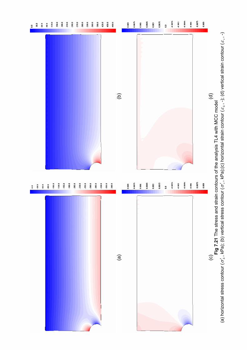
(a
)
(b)
(c
)
(d)
Fig
7.21
The
stre
ss a
nd s
train
con
tour
s of
the
anal
ysis
TL4
with
MC
C m
odel
(a
) hor
izon
tal s
tress
con
tour
(h
σ′ ,
kP
a); (
b) v
ertic
al s
tress
con
tour
(v
σ′ ,
kP
a);(c
) hor
izon
tal s
train
con
tour
(hε, -
); (d
) ver
tical
stra
in c
onto
ur (
vε, -
)
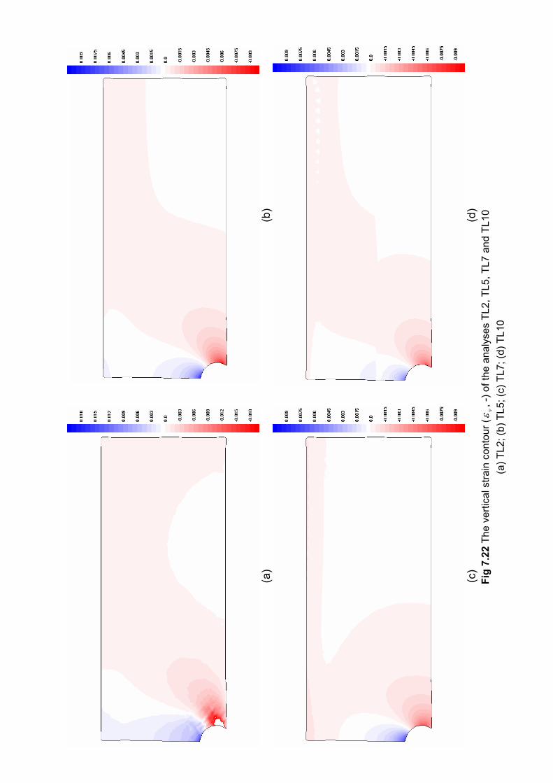
(a
)
(b)
(c
)
(d)
Fig
7.22
The
ver
tical
stra
in c
onto
ur (
vε, -
) of t
he a
naly
ses
TL2,
TL5
, TL7
and
TL1
0 (a
) TL2
; (b)
TL5
; (c)
TL7
; (d)
TL1
0
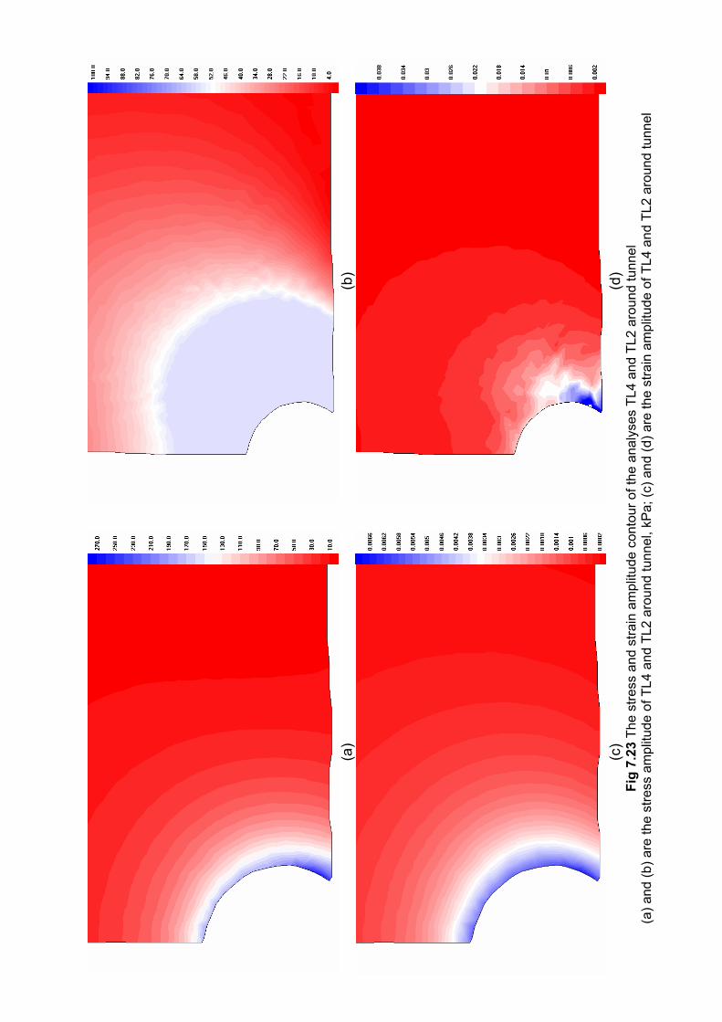
(a
)
(b)
(c
)
(d)
Fig
7.23
The
stre
ss a
nd s
train
am
plitu
de c
onto
ur o
f the
ana
lyse
s TL
4 an
d TL
2 ar
ound
tunn
el
(a) a
nd (b
) are
the
stre
ss a
mpl
itude
of T
L4 a
nd T
L2 a
roun
d tu
nnel
, kP
a; (c
) and
(d) a
re th
e st
rain
am
plitu
de o
f TL4
and
TL2
aro
und
tunn
el

(a
)
(b)
(c
)
(d)
Fig
7.24
The
nod
al fo
rce
and
disp
lace
men
t vec
tor o
f the
ana
lyse
s TL
4 w
ith M
CC
mod
el
(a) a
nd (c
) are
nod
al fo
rce
and
disp
lace
men
t vec
tor r
espe
ctiv
ely;
(b) a
nd (d
) are
nod
al fo
rce
and
disp
lace
men
t vec
tor a
roun
d th
e tu
nnel
Application to geotechnical problems
7-33
Figures 7.24(a) and (b) show the nodal force vectors for all nodal points around
the tunnel in analysis TL4. The nodal forces for all analyses should be the same
because they are constrained by the same boundary and ground conditions. The
surface boundary corresponds to the applied surcharge load. Both side boundaries
utilise the roller support condition. The nodal forces at the bottom boundary conform
with the total reaction force due to the gravity load and the applied surcharge load.
The nodal force around the lining presents the reaction of the concrete lining
subjected to the simulated internal pressure. The nodal displacement vector for all
nodal points in analysis TL4 is shown in Figures 7.24(c) and (d). The nodal
displacements are concentrated around the tunnel and reduce to small values in the far
field. All displacements are toward to the tunnel as expected. The movements are
significant at the crown and decrease towards the springline.
7.3 Conclusion These two exercises on finite element analysis are presented in this chapter to
illustrate the soil models as applied to Bangkok clay. The road embankment problem
is related to the strength of the soft ground. The problem is analysed under two-
dimensional plane strain conditions in order to reduce the amount of calculation.
Using 449 six-noded triangular elements is sufficient to model a ground block. The
undrained analysis can be only carried out using the EVM model (EM1 and EM2)
because of the limitation of OXFEM code. For the rest of the analyses (EM3 to
EM11), drained condition are analysed using the EVM, MCC and KHMCC models.
The analyses found that the strength does not vary too much among the constitutive
laws, whereas the deformation shape depends much on the constitutive law. The
analysis results exhibit a smooth distribution of stresses and strains as shown in the
contour plots. These two-dimensional analyses concern some factors such as surface
crust and K0. The effect of a surface crust makes the settlement profile slightly
shallower due to the higher stiffness of the overconsolidated state of the crust layer.
The reduction of K0 from 1.0 to 0.7 makes the settlement profile much deeper. The
approximation of the soil embankment by nodal forces can be reasonably assumed.
However, the triangular embankment should be replaced by not only the vertical
nodal force but also the horizontal nodal force. The analysis considering the effect of
lateral load discovered that the effect can be disregarded, because the horizontal load
is relatively small compared with the load from whole embankment.
Application to geotechnical problems
7-34
The critical problem for the tunnel is not the strength of soil but rather the
excessive settlement trough. An empirical formulation to predict tunnelling-induced
settlement is widely used in practice. However, there is no better solution than finite
element analysis to calculate the stress-strain behaviour around a tunnel. In this study,
the tunnel is simulated as a two-dimensional plane strain problem with 1105 six-
noded triangular elements, analysed by using three different models i.e. the EVM,
MCC and KHMCC models. The undrained analysis can only be analysed using the
EVM model (TL1 and TL2) and the other analyses (TL3 to TL11) are carried out in
drained conditions. The comparisons of the settlement trough prediction found that
all predicting troughs except TL2 are consistent with the empirical formula and the
field data. However, this cannot guarantee the accuracy of all models since only one
set of field data is used for comparison. The analyses with a reduction of K0 show
deeper and narrower troughs as expected. A discontinuity of the stress-strain contours
is found from the two layer analyses, and this is due to the sudden change of stiffness
from soft to stiff.
For the embankment problem with 449 nodes, the analysis time is roughly about
30 minutes whereas it is spent almost 2 hours for the tunnelling problem with 1105
nodes. The running time of the analysis with KHMCC model using 50 yield surfaces
is slightly longer than the MCC case (single yield surface) about 10-20%. This is
implied that the analysis time mainly uses for the global load-deformation matrix
operation rather than the updating of the stress-strain at element level. The former is
controlled by size of problems, but the latter depends on the choice of constitutive
model used.
However, these two examples of analysis prove the ability of soil model to be
employed in practice. In further analysis, more complicated factors need to be dealt
with, such as consolidation analysis, because the limitation on total stress calculation
in the present version of OXFEM is constrained to analyse problems for only fully
undrained or drained conditions.

Concluding remarks
8-1
Chapter 8 Concluding Remarks
8.1 Summary of research Research at Oxford University on constitutive modelling for soils concentrates
principally on the use of plasticity theory for building soil models. In much of the
recent work there has been an emphasis on the use of thermodynamic principles to
develop a new approach to plasticity modelling termed hyperplasticity. This project
is a programme of development of practical soil models, especially clay models,
based on hyperplasticity theory.
There are many soil models with their authors each claiming their advantages
over other soil models. There is still no explicit model which explains fully the
behaviour of soil subjected to general construction processes. Since some of the
models are based on laboratory research and are described in terms of sophisticated
expressions, they are rarely used in practice. This project tries to develop a practical
constitutive soil model to employ in geotechnical work. The research tasks can be
separated into three main areas:
(i) building a theoretical soil model based on the hyperplasticity concept,
(ii) evaluation the soil model parameters based on experimental data, and
(iii) implementation of the soil model in a finite element program.
8.1.1 Theoretical soil models The most important feature of the new approach is that the entire constitutive
behaviour can be derived from two scalar potentials. Applying the hyperplasticity
idea to soil models, the kinematic hardening model is selected as a key stage in
developing a model with a continuous internal functional. The continuous kinematic
hardening functional model can accommodate a smooth transition of stiffness during
unloading and reloading below the maximum past stresses. While the continuous
hyperplasticity approach can offer a continuous smooth stress-strain response, in
numerical applications, the continuous function has to be replaced by a series of
piecewise linear functions, which are implemented in terms of multiple internal
variables.
Concluding remarks
8-2
This research develops a new constitutive model for soil mechanics that makes
use of two underlying stress-strain relationships: linear and logarithmic. At this stage,
the development of research is directed to an elasto-plastic model with a continuous
hardening function in terms of triaxial stress-strain parameters. The ultimate model is
called kinematic hardening modified Cam-clay model (KHMCC), which requires
eight parameters (for linear stiffness), or seven parameters (for logarithmic stiffness)
plus one parameter ( )µ for rate-dependence.
8.1.2 Evaluation of model parameters In order to evaluate the model parameters, the experimental data for Bangkok
clay obtained from Asian Institute of Technology (AIT) and Chulalongkorn
University are employed. The experimental data at both the small strain level and
large strain are required to explain the variation of stiffness from small to large strain
levels. The AIT data contains information on triaxial tests at large strain level. On
the other hand, the small strain data is provided by the research on cyclic undrained
shear at Chulalongkorn University.
Based on the results of the study, the linear stress-strain model is proposed for
this study. All predictions are simulated by assuming uniform stress-strain
distribution in axi-symmetry conditions. Every sample is consolidated following its
stress history and sheared in its specific condition such as undrained, drained or cyclic
undrained condition where the rate effects are concerned. Utilising these results,
model parameters for Bangkok clay are proposed.
8.1.3 Implementation of software From a numerical aspect, an incremental response calculation is required to
evaluate the stress-strain response. There are two calculation algorithms (i.e. rate-
independent and rate-dependent) considered here. These two algorithms are initially
implemented using FORTRAN 90 for the triaxial calculation. Further development of
soil models in the form of generalised stress-strain parameters is performed to link the
model to the OXFEM finite element program. This research considers special
conditions, such as two-dimensional plane strain and axi-symmetry. The model
requires the transformation from generalised stress-strain to two-dimensional stress-
strain relation.

Concluding remarks
8-3
The calculation of global incremental load-deformation behaviour has to deal
with a slightly more complicated algorithm than the incremental stress-strain in a
single element calculation. The present version of OXFEM employs the Newton-
Raphson (NR) algorithm. Before starting the analysis, some triaxial problems are
tested to make sure that the subroutines developed and the link between the old code
and new subroutine are correct.
8.1.4 Applications Two application examples of geotechnical construction are selected: analysis
of a road embankment and estimation of tunnelling-induced settlement. The problems
are simplified into two-dimensional plane strain conditions, and symmetry is used to
reduce the amount of calculation. The mesh is generated using the I-DEAS
commercial programme. These finite element analyses are calculated using OXFEM
including the subroutines developed by the author. All analyses are carried out using
three constitutive models: elastic Von Mises (EVM), modified Cam-clay (MCC) and
kinematic modified Cam-clay (KHMCC) model. The model parameters are
employed from the parameters derived from laboratory testing except in the EVM
model, which have been estimated from the MCC parameters.
8.2 Conclusions The conclusions from this research can be summarised as follows:
1. The KHMCC model is categorised as a multiple yield surface model. However,
there is another idea called bounding surface plasticity which addresses some of the
weak points of critical state soil models. Although the bounding surface concept,
such as in the MIT-E3 model (Whittle, 1993), offers efficient computation and a
sufficiently accurate prediction of stress-strain-strength behaviour, there are still two
major drawbacks. The bounding surface concept requires some arbitrary functions
(such as a mapping rule and a hardening rule) without obvious physical meaning, and
the concept cannot explain the effect of immediate past history such as a hysteresis
loop on unloading-reloading. These two deficiencies can be described by the multiple
yield surface idea. There are also some disadvantages of the multiple yield surface
model; for example the nested yield surface model (Mroz et al., 1982). The multiple
yield surface model requires a considerable amount of calculation in each yield
surface and needs a large number of hardening parameters. These problems can be

Concluding remarks
8-4
eliminated by introducing a functional (loosely defined as function of a function).
This mathematical framework provides the concept that all yield surfaces are reduced
to a single structure with different sizes and a large number of kinematic parameters
are replaced by a function. These have been included in the current research.
2. A bubble model (Al Tabbaa and Wood, 1989) applies the kinematic hardening idea
to the MCC model. An improvement on the bubble model, to consider the effect of
immediate stress history, has been explored in the three-surface kinematic hardening
(3-SKH) soil model (Atkinson and Stallebrass, 1991). This model was intended to
improve the original bubble model by adding an extra intermediate yield surface in
order to deal with moderate strain levels. However, there is still a question whether it
is logical to limit the number of multiple yield surfaces to three surfaces. The models
cannot produce the response to cyclic loading behaviour which has a small change of
stress amplitude. These models could be extended to an infinite number of yield
surfaces. This can be dealt with by using a continuous functional which provides a
mathematical framework for generating a smooth curve. This concept has been
applied in the KHMCC model.
3. All recent soil models aim to generate plasticity behaviour inside the SBS which
could not be achieved by the MCC model. Some models contain many advantages of
theories such as anisotropic yield surface, hysteretic formulation and process of
destructuration. Therefore, they give a better quality in term of laboratory prediction.
However, these theories make the model too sophisticated. They are rarely used in
practice. This research tries to link between the theoretical and practical sides.
Although the new model does not give the best predictive qualities, it can resolve
some of the weak points that cannot be explained by other models.
4. In order to define the continuous kinematic hardening model, we need an
expression for the kinematic hardening function, which relates to the observed stress-
strain curve. This process involves much trial and error in order to define the
mathematical formulae. The research leads to a recommendation for a hyperbolic
function. The hyperbolic shape is controlled by four parameters (i.e. E, a, b and r
referred to equation 3.38), which have physical meaning. The initial slope of the
curve (E) refers to the elastic modulus while the asymptotic slope (related to

Concluding remarks
8-5
parameter r) defines the plastic modulus. The remaining parameters (a and b), which
control rate of change of slope, can be evaluated by the definition of secant modulus
and/or tangential modulus at particular stresses.
5. Both numerical approaches to determine the incremental stress-strain (rate-
independent and rate-independent) are implemented. The rate-independent
calculation requires some consistency conditions which involve a higher complexity
of computation than rate-dependence. It also requires some error control that the
rate-dependent algorithm does not need. The most obvious benefit of the rate-
dependent calculation is the inclusion of rate dependency for materials which can
exhibit any significant rate effects. In addition, for the rate-independent approach, the
updated strain increment, consistency condition, hardening rule as well as the error
controls are included in the governing matrix. In contrast, only the updated strain
increment appears in the governing matrix for the rate-dependent calculation.
Therefore, the algorithm for rate-independence has to deal with larger sizes of
governing matrix than the rate-dependent. As a result, the rate-dependence reduces
the computing time considerably.
6. The KHMCC model prediction of consolidation behaviour is more accurate than
its prediction of other behaviours. This is because the consolidation prediction only
acts on the p term of the model but does not deal with the p-q coupling term. The
prediction of pure shear behaviour (i.e. CID-90 and CID-270) can be used to estimate
critical state parameters (MC, ME). However, ME is normally slightly higher than MC.
For simplicity, the assumption of EC MM = is made in this research. The isotropic
consolidated drained tests are accurately predicted in terms of stress path and shear
strength using KHMCC model. On the other hand, the anisotropic consolidated
drained predictions are slightly inaccurate, especially in terms of stress path. The
prediction of the variation of shear stiffness is relatively accurate for both isotropic
and anisotropic consolidated tests. The simulation of the cyclic undrained tests gives
accurate results. The variation of the shear modulus and the damping ratio are
accurately simulated by the KHMCC model. The main advantage of the model is that
it can predict both the monotonic loading and cyclic loading response by the same
constitutive law.

Concluding remarks
8-6
7. The road embankment problem based on the field data from the Bangkok project
was selected as the first problem for study of a geotechnical application. The most
critical issue of embankments on soft clay is the strength of soft ground during the
construction period, as a low undrained shear strength cannot resist the high
embankment load. The analyses discovered that the stress fields do not vary much
among the constitutive soil models. Although, this study does not predict the
undrained behaviour with the soil models used, the drained long-termed settlement
prediction is calculated. This restriction in the analysis comes from a constraint of the
present version of the OXFEM finite element program, in which it does not include
code dealing with consolidation analysis. The comparison of the settlement profile
with field data can not be made, because only a single settlement point at each road
section was recorded. In addition, this series of two-dimensional analyses also
includes studies of some aspects of the embankment problem such as the effect of a
surface crust, K0 and lateral shear force. The effect of a surface crust makes the
ground response stiffer. On the other hand, the ground response is softer when the K0
is reduced. Theoretically, the lateral shear force must be included in the nodal force
for the embankment analysis. However, the research found that this effect can be
disregarded according to the small effect of lateral load compared with the whole size
of the embankment.
8. The second geotechnical problem considered in this study is the biggest public
transportation underground tunnel in Bangkok named MRTA. The important
problem of the tunnel is not the strength of soil but the excessive settlement trough.
The series of two-dimensional analyses also include some modifications to the ground
such as anisotropic ground (reduction of K0) and layered ground. The analyses found
that the displacement fields depend much on the models used. The result of analysis
with the KHMCC model offers a better transition of stress-strain than the MCC
model. The reduction of K0 leads to an increase in the vertical strains which lead to a
deeper and narrower settlement trough. The two-layer analyses show a discontinuity
of the stress contour at the boundary between soft and stiff clay due to the sudden
change of stiffness from the soft to stiff layer.
9. From the analyses of two geotechnical problems, it can be concluded that for the
analysis of the strength problem it is not necessary to utilise an advanced soil model.
Concluding remarks
8-7
The models such as the EVM and the MCC model can also provide a sufficient
strength prediction. In contrast, for the analysis of displacement problem, the
advanced soil models which give a transition of stiffness from small strain to large
strain level are recommended. The KHMCC model is therefore one of the possible
soil models used to predict this problem. The effect of past stress history and K0 can
also be described by the KHMCC model.
8.3 Recommendations Research on constitutive models for soils requires further work. Some
recommendations for future research are as follows:
1. To improve the stress-strain response, the continuous hardening function ( ( )ηH )
should be modified to generate a better stress-strain curve. The present version of the
KHMCC model assumes the stress-strain curve to be hyperbolic. Other forms of
continuous hardening function might be introduced.
2. The fact that soils are likely to be anisotropic, with their behaviour depending on
the direction of deposition, is important. The multiple yield surface concept can
accommodate the anisotropic behaviour by means of memorisation of the yield
surface locations from the past stress history. However, this is still not sufficient to
explain the experimental results. To improve this, the model should introduce other
yield criteria or/and anisotopic yield surface shape. Firstly, this is because the yield
criteria such as the Matsuoka-Nakai criterion offer a smooth change of yield strength
in the deviatoric plane. In the Matsuoka-Nakai criterion, the magnitude of critical
state cone will depend on where the stress state is in the deviatoric plane. Secondly,
the anisotropic yield surface shape, e.g. the deformed elliptical shape or the rotating
elliptical shape, is believed to be able to describe the anisotropic behaviour.
3. The laboratory investigation shows that every sheared sample is not necessarily
enforced to reach the same critical state as stated in the CSSM assumption. This is
especially the case for samples on the dry side of CSL. An improvement of the model
prediction should introduce some ideas to account for the aforementioned
phenomenon. The concepts of localisation and strain softening are believed to be able
to explain the behaviour of heavily overconsolidated clay. The localisation idea

Concluding remarks
8-8
assumes that all material elements do not necessary reach the yield state at the same
time. The material consists of both an elastic zone and a shear band (plastic zone),
where the ratio of these two volumes controls the material behaviour. In contrast,
strain softening allows the yield surface to move inward or reduce its size when the
stress state touches yield surface.
4. Although the cyclic undrained triaxial tests are predicted quite well by the KHMCC
model, the prediction of behaviour of soil at small strain level needs still to be
improved in future research. Experimental results for the Bangkok clay at small strain
levels from apparatus such as a directional shear cell and hollow cylinder are
currently unavailable.
5. Development of rate process theory (Houlsby and Purzin, 2002) could provide
improvements to the prediction of short-term consolidation behaviour (before the end
of primary consolidation) as well as long term creep behaviour.
6. A constraint of the present version of the OXFEM finite element program is that it
does not include the code dealing with consolidation analysis. Thus, the consolidation
code should be added in the OXFEM program.
7. In future analyses, the use of techniques other than the Newton-Raphson (NR)
method for solution of the incremental load-deformation is recommended to improve
the running speed and/or accuracy, particularly for larger size problems including
three-dimensional analyses.
This research aims to build a new constitutive soil model, in particular clay
model. Based on the continuous hyperplasticity concept, the research produces a
satisfied model which can generate the smooth transition behaviour from elastic to
plastic. Although the model does not substantially improve the prediction qualities, it
can describe the effects of immediate stress history which is a strong point of the
model. The model also includes the rate effect which is useful for the analysis of a
staged construction process. Two geotechnical applications of the model confirm
that it is undoubtedly used for the geotechnical engineering.

References
9-1
REFERENCES Addenbrooke, T.I., Potts, D.M., and Puzrin, A.M. (1997), “The influence of pre-failure soil stiffness on the numerical analysis of tunnel construction”, Geotechnique, Vol. 47, No. 3, pp. 693-712 Al-Tabbaa A. and Wood D.M. (1989), “An experimentally based ‘bubble’ model for clay”, Pro. of Int. Conf. Numerical models in geomechanics NUMOG 3, Edt. Pietruszczak and Pande, Balkema, pp 91-99 Atkinson, J.H., Richardson, D., and Stallebrass, S.E. (1990), “Effect of recent stress history on stiffness of overconsolidated soil”, Geotechnique, Vol. 40, pp. 531-540 Atkinson, J.H. and Sallfors, G. (1991), “Experimental determination of stress-strain-time characteristics in laboratory and in-situ tests”, Proc. of X ECSMFE, Florence, (Eds. Associazione Geotecnica Italiana), pp 915-956 Rotterdam: A. A. Balkema Atkinson, J.H. and Stallebrass, S.E. (1991), “A model for recent stress history and non-linearity in the stress-strain behaviour of overconsolidated soil”, Proc. 7th Int. Cof. On Computer Methods and Advances in Geomechanics, Cairns, Vol. 1, pp555-560 Augarde, C.E. (1997), “Numerical modelling of tunnelling processes for assessment of damage to buildings”, D.Phil. Thesis, University of Oxford Augarde, C.E. and Burd, H.J. (2001), “Three-dimensional finite element analysis of lined tunnels”, Int. J. Numer. Anal. Meth. Geomech., Vol. 25, pp 243-262 Bloodworth, A.G. (2002), “Three-dimensional analysis of tunnelling effects on structures to develop design method”, D.Phil. Thesis, University of Oxford Burd, H.J. (1986), “A large displacement finite element analysis of a reinforced unpaved road”, D.Phil. Thesis, University of Oxford Butterfield, R. (1979), “A natural compression law for soils (an advance on e-log p′ )”, Geotechnique, Vol. 29, No.4, pp 469-480 Coleman, B.D. and Gurtin, M.E. (1967), “Thermodynamics with internal state variables”, J. Chem. Phys. Vol. 47, pp. 597-613 Collins, I.F. and Houlsby G.T. (1997), “Application of thermomechanical principles to the modelling of geotechnical materials”, Proc. Royal Society of London, Series A, Vol. 453, pp 1975-2001 Dafalias, Y. and Herrmann, L.R. (1982), “Bounding surface formulation of soil plasticity”, Soil Mechanics Cyclic and Transient Loads (G. N. Pande and O. C. Zienkiewicz, eds), Chapter 10, pp 253-282, New York, John Wiley & Sons Drucker, D. C. and Prager, W. (1952), "Soil Mechanics and plastic analysis or limit design", Quarterly of Applied Mechanics, Vol. 10(2), pp. 157-165
References
9-2
Einav, I., Puzrin, A.M and Houlsby, G.T. (2000), “Continuous hyperplastic models for overconsolidated clays”, Proc. Symp. on Mathematical Models in Geomechanics, Scilla di Reggio Calabria, 19-22 Sept., Vol. 37, No. 5/6, pp 515-523 Graham, J. and Houlsby, G.T. (1983), “Anisotropic elasticity of a natural clay”, Geotechnique, Vol. 33, No. 2, pp165-180 Gurung, S.B. (1992), “Yielding of soft Bangkok clay below the boundary surface under compression conditions”, M. Eng. Thesis, GT-91-11, AIT, Bangkok Hashiguchi, K. (1985), “Two- and Three-surface models of plasticity”, Proc. 5th Int. Cof. Numerical Methods in Geomechancis, Nagoya, pp 285-292 Houlsby, G.T. (1999), “A model for the variable stiffness of undrained clay”, Proc. Int. Symp. on Pre-Failure Deformation of Soils, Torino, 26-29 September, Balkema, ISBN 9058090760, Vol. 1, pp 443-450 Houlsby, G.T. and Puzrin, A.M. (1999), “An approach to plasticity based on generalised thermodynamics”, Proc. of the International Symposium on Hypoplasticity, Horton, Greece, pp 233-245 in press Houlsby, G.T. and Puzrin, A.M. (2000), “A thermomechanical framework for constitutive models for rate-independent dissipative materials”, International Journal of Plasticity, Vol. 16 No. 9, pp 1017-1047 Houlsby, G.T. and Puzrin, A.M. (2002), “Rate-dependent plasticity models derived from potential functions”, Journal of Rheology, Vol. 46, No. 1, pp 113-126. Howatson, A.M., Lund, P.G., and Todd, J.D. (1991), “Engineering tables and data”, Chapman & Hall, London Hueckel, T. and Nova, R. (1979), “Some hysteresis effects of the behaviour of geologic media”, International Journal of Solids and Structures, Vol. 15, pp. 625-642 Iwan, W.D. (1967), “On the class of models for the yielding behavior of continuous and composite systems”, Transactions of the American Society of Mechanical Engineers, Journal of Applied Mechanics, Vol. 34, pp 612-617 Khan, M.R.A. (1999), “Stress-strain behaviour of soft Bangkok clay below the state boundary surface under anisotropic conditions”, M. Eng. Thesis, AIT Bangkok Kim, S.R. (1991), “Stress-strain behaviour and strength characteristics of lightly overconsolidated clays”, Doctoral Dissertation, GT-90-2, AIT, Bangkok Kolymbas, D. (1977), “A rate-dependent constitutive equation for soils”, Mech. Res. Comm., Vol. 4, pp. 367-372 Lee, K.M. and Rowe, R.K. (1989), “Deformations caused by surface loading and tunnelling: the role of elastic anisotropy”, Geotechnique, Vol. 39, No. 1, pp. 125-140

References
9-3
Likitlersuang, S. (2000), “Elasto-plastic analysis of soft clay behaviour”, M. Eng. Thesis, AIT, Bangkok Lin, D.G., Tseng, C.T., Phienwej, N., and Suwansawat, S. (2002), “3-D deformation analysis of earth pressure balance shield tunnelling in Bangkok subsoil”, Journal of Southeast Asian Geotechnical Society, Vol. 33, April 2002, pp13-27 Liu, G. (1997), "Numerical modelling of damage to masonry buildings due to tunnelling" D.Phil. Thesis, University of Oxford Lubliner, J. (1972), “On the thermodynamic foundation of non-linear solid mechanics”, Int. J. of Non-linear Mechanics Matsuoka, H. and T. Nakai (1974), “Stress-deformation and strength characteristics of soil under three different principal stresses” Proceedings, JSCE, no. 232, Dec, 1974, pp. 59-70 Mitchell, J.K. (1976), “Fundamentals of soil behavior”, John Wiley and Sons, New York Mroz, Z. (1967), “On the description of antisotropic workhardening”, J. Mech. Phys. Solids, Vol. 15, pp. 163-175 Mroz, Z. and Norris, V.A. (1982), “Elastoplastic and viscoplastic constitutive models for soils with application to cyclic loading”, Soil Mechanics Cyclic and Transient Loads (G. N. Pande and O. C. Zienkiewicz, eds), Chapter 8, pp 173-218, New York, John Wiley & Sons Navaneethan, T. (1999), “Extension behaviour of soft Bangkok clay with selected applied stress paths”, M. Eng. Thesis, AIT, Bangkok O'Reilly, M. P. and New, B. M. (1991), “Tunnelling induced ground movements; predicting their magnitude and effects”, 4th International Conference on Ground Movements and Structures, Cardiff invited review paper, Pentech Press, pp.671-697 Pestana, J.M. and Whittle, A.J. (1999), “Formulation of a unified constitutive model for clays and sands”, International Journal for Numerical and Analytical Methods in Geomechanics, Vol. 23, pp. 1215-1243 Potts, D.M. and Zdravkovic, L. (1999), “Finite element analysis in geotechnical engineering Volume I, II”: Theory and Application, Tomas Telford, ISBN 0727727532 Prevost, J.H. (1978), “Plasticity theory for soil stress-strain behaviour”, Proceedings of the American Society of Civil Engineers, Journal of the Engineering Mechanics Division, Vol. 104, No. EM5, October, pp 1177-1194

References
9-4
Puzrin, A.M. and Burland, J.B. (1996), “A logarithmic stress-strain function for rocks and soils”, Geotechnique, Vol. 46, No. 1, pp 157-164 Puzrin, A.M. and Burland, J.B. (1998), “Non-linear model of small-strain behaviour of soils”, Geotechnique, Vol. 48, No. 2, pp 217-233 Puzrin, A.M. and Houlsby, G.T. (2001a), “Strain-based plasticity models for soils and the BRICK model as an example of hyperplasticity approach”, Geotechnique, Vol. 51, No. 2, pp 169-172 Puzrin, A.M. and Houlsby, G.T. (2001b), “Fundamentals of kinematic hardening hyperplasticity”, International Journal of Solids and Structures, Vol. 38, pp 3771-3794 Puzrin, A.M. and Houlsby, G.T. (2001c) “On the non-intersection dilemma in multi-surface plasticity”, Geotechnique, Vol. 51, No. 4, pp 369-372 Puzrin, A.M. and Houlsby, G.T. (2001d), “A thermomechanical framework for rate-independent dissipative materials with internal functions”, International Journal of Plasticity, Vol. 17, pp 1147-1165 Puzrin, A.M. and Houlsby, G.T. (2003), “Rate-dependent hyperplasticity with internal functions”, Proceedings of the American Society of Civil Engineers, Journal of the Engineering Mechanics Division, Vol. 129, No. 3, March, pp 252-263 Roscoe, K. H., Schofield, A. N. and Thurairajah, A. (1963), "Yielding of clays in state wetter than critical" Geotechnique, Vol. 13, No. 3, pp. 211-240 Roscoe, K.H. and Burland, J.B. (1968), “On the generalised behaviour of ‘wet’ clay”, Engineering Plasticity, (Heyman, J. and Leckie, F.A. eds.), Cambridge University Press, pp. 535-610 Rouainia, M. and Wood, D.M. (2000), “A kinematic hardening constitutive model for natural clays with loss of structure”, Geotechnique, Vol. 50, No. 2, pp. 153-164 Schofield, A.N. and Wroth, C.P. (1968), “Critical state soil mechanics”, McGraw Hill, London Seah, T.H. (1990), “Anisotropy of normally consolidated Boston blue clay”, Sc.D. Thesis, MIT. Seah, T.H. (1998), “Differential settlements in highway no. 34 pavement caused by construction of Bangna-Bangpli-Bangpakong expressway”, Report submitted to Expressway Transit Authority of Thailand Seah, T.H. and Juirnarongrit, T. (1999), “Constant rate of strain consolidation with radial drainage”, in press Seah, T.H. and Hassan, S.I. (1999), “Constant rate of strain consolidation testing on Bangkok clay”, in press

References
9-5
Soga, K., Nakagawa, K., and Mitchell, J.K. (1995), "Measurement of stiffness degradation characteristics of clays using a torsional shear device", First International Conference on Earthquake Geotechnical Engineering, Tokyo, Nov. 14-16, pp. 107-112 Stallebrass, S.E., Jovicic, V. and Taylor, R.N. (1994), “The influence of recent stress history on ground movements around tunnels”, Pre-failure Deformation of Geomaterials (Shibuya, Mitachi and Miura eds), pp 615-620, Balkema, Hotterdam, ISBN 905410399 Stallebrass, S.E. and Taylor, R.N. (1997), “The development and evaluation of a constitutive model for the prediction of ground movements in overconsolidated clay”, Geotechnique, Vol. 47, No. 2, pp. 225-253 Teachavorasinskun, S., Thongchim, P., and Lukkunaprasit, P. (2001), “Shear modulus and damping ratio of clay during undrained cyclic loading”, Geotechnique, Vol 51, No. 5, pp 467-470 Teachavorasinskun, S., Thongchim, P., and Lukkunaprasit, P. (2002), “Stress rate effect on the stiffness of a soft clay from cyclic”, compression and extension triaxial tests, Geotechnique, Vol. 52, No. 1, pp 51-54 Tuladhar, L. (2000), “Behaviour of soft clay below the state boundary surface with stress Paths from extension to compression”, M. Eng. Thesis, AIT, Bangkok Uchaipichat, A. (1998), “Triaxial tests on soft Bangkok clay with different applied stress paths”, M. Eng. Thesis, GT-97-13, AIT, Bangkok Vaid, P. and Campanella, R.G. (1974), “Triaxial and plane strain behaviour of natural clay”, Journal of Geotechnical Engineering, ASCE, Vol. 100, No.3, pp 207 Whittle, A.J. (1993), “Evaluation of a constitutive model for overconsolidated clays”, Geotechnique, Vol. 43, No. 2, pp 289-313 Whittle, A.J., DeGroot, D.J., Ladd, C.C., and Seah, T.H. (1994), “Model prediction of anisotropic behaviour of Boston Blue Clay”, Journal of Geotechnical Engineering, ASCE, Vol. 120, pp 199-224 Wood, D.M. (1995), “Kinematic hardening model for structured soil”, Numerical models in geomechanics NUMOG 5 (Eds. G.N. Pande & S. Pietruszczak), pp 83-88 Rotterdam: A. A. Balkema Zdravkovic, L., Potts, D.M., and Jardine, R.J. (2001), “A parametric study of the pull-out capacity of bucket foundations in soft clay”, Geotechnique, Vol. 51, No. 1, pp. 55-67 Zdravkovic, L., Potts, D.M., and Hight D.W. (2002), “The effect of strength anisotropy on behaviour of embankments on soft ground”, Geotechnique, Vol. 52, No. 6, pp 447-457

References
9-6
Ziegler, H. (1983), “An introduction to thermomechanics”, North Holland, Amsterdam

Appendices
A-1
APPENDIX A This following section lists the new input modules for OXFEM. These will be
included in the OXFEM manual. The new input modules are for specifying two
material types, initial states and rate-dependent calculation.
Material properties
*MATERIALS
For mtyp = 9; Kinematic Hardening Modified Cam Clay model (KHMCC)
Property number (in
specification list) Constant properties Descriptions
p1 K Initial bulk modulus
p2 ap
p3 bp
p4 r
Non-linear kinematic hardening
parameter in isotropic (p) direction
p5 gx Elastic shear modulus gradient
p6 aq
p7 bq
Non-linear kinematic hardening
parameter in deviatoric (q) direction
p8 M Slope of critical state line
p9 µ Viscosity coefficient (for rate-
dependent calculation) For mtyp = 12; Modified Cam Clay model (MCC)
Property number
(in specification list) Constant properties Physical meaning
p1 κ∗ Slope of swelling consolidation line on
log v-log p plot
p2 λ∗ Slope of virgin consolidation line on
log v-log p plot
p3 gx Elastic shear modulus gradient
p4 M Slope of critical state line
p5 µ Viscosity coefficient (for rate-
dependent calculation)
p6 px0 Reference stress of initial yield surface Specification of initial states
*INITIAL_STATE
max1max1111 vhvhz σσσσ
max2max2222 vhvhz σσσσ

Appendices
A-2
… etc.
This module follows the *INTIAL module which contains information about initial
stresses in the order of vh σσ , (initial horizontal and vertical stress) and also includes
the information of stress history in the order of maxmax , vh σσ (maximum past horizontal
and vertical stress).
Calculation information
*CALCULATION_TIME
filename
nstep1 tol1 time1
nstep2 tol2 time2
… etc.
The CALCULATION module contains calculation information especially for rate-
independent model. In order to provide the rate-dependent calculation, timei
(calculation time in ith loading stages) is introduced into the
CALCULATION_TIME module.

Appendices
A-3
APPENDIX B !******************************* MCC - Subroutine ***************************************! ! ! This file contains a range of subroutines for a Modified Cam Clay model. These ! routines have been written by Suched Likitlersuang. Feb 2003 !********************************* Mathematic Definition**************************************! double precision function ilog(x) ! ~~~~~~~~ Integration of log(x) use utils implicit none real (kind=dp), intent(in) :: x ilog=x*log(x)-x end function ilog !******************************** Constitutive Equation **************************************! subroutine makeAA_MCC(STRESS,PROP,alpha,AA) ! ~~~~~~~~~ Elastic Compliance (d2g/dsigma2) use utils use maxdim use values implicit none real (kind=dp), intent(in) :: STRESS(MSTR),PROP(MPROP),alpha(MSTR) real (kind=dp), intent(out) :: AA(MSTR,MSTR) real (kind=dp), external :: delta real (kind=dp) :: kappa,gx,p,divSTS(MSTR),divSTS2 integer :: iSTR,jSTR kappa = PROP(1) gx = PROP(3) p = (STRESS(1)+STRESS(2)+STRESS(3))/3.0d0 divSTS2=0.0d0 do iSTR=1,MSTR divSTS(iSTR)=STRESS(iSTR)-p*delta(iSTR) if (iSTR==4) then divSTS2=divSTS2+2*divSTS(iSTR)**2 else divSTS2=divSTS2+divSTS(iSTR)**2 end if end do do iSTR=1,MSTR do jSTR=1,MSTR if ((iSTR<=3).and.(jSTR<=3)) then if (iSTR==jSTR) then AA(iSTR,jSTR)=(kappa/(9.0d0*abs(p)))+(1.0d0/(3.0d0*gx*abs(p))) & +(divSTS2/(18.0d0*gx*abs(p)**3))-(divSTS(iSTR)/(3.0d0*gx*p**2)) else AA(iSTR,jSTR)=(kappa/(9.0d0*abs(p)))-(1.0d0/(6.0d0*gx*abs(p))) & +(divSTS2/(18.0d0*gx*abs(p)**3))-((divSTS(iSTR)+divSTS(jSTR))/(6.0d0*gx*p**2)) end if else if ((iSTR<=4).and.(jSTR<=4)) then if ((iSTR==4).and.(jSTR==4)) then AA(iSTR,jSTR)=1.0d0/(gx*abs(p)) else AA(iSTR,jSTR)=-STRESS(4)/(3.0d0*gx*p**2) end if else AA(iSTR,jSTR)=0.0d0 end if end do end do end subroutine makeAA_MCC subroutine makeBB_MCC(STRESS,alpha,BB) ! ~~~~~~~~~ Stress-plastic coupling term (d2g/dalphadsigma) use utils use maxdim use values implicit none real (kind=dp), intent(in) :: STRESS(MSTR),alpha(MSTR) real (kind=dp), intent(out) :: BB(MSTR,MSTR) real (kind=dp), external :: delta integer :: iSTR,jSTR do iSTR=1,MSTR do jSTR=1,MSTR if (iSTR==jSTR) then BB(iSTR,jSTR)=1.0d0

Appendices
A-4
else BB(iSTR,jSTR)=0.0d0 end if end do end do end subroutine makeBB_MCC subroutine makeCC_MCC(STRESS,PROP,alpha,CC) ! ~~~~~~~~~ Plastic Rate-dependent (dw/dchi) use utils use maxdim use values implicit none real (kind=dp), intent(in) :: STRESS(MSTR),PROP(MPROP),alpha(MSTR) real (kind=dp), intent(out) :: CC(MSTR) real (kind=dp), external :: macaulay,delta real (kind=dp) :: kappa,lambda,gx,M,px0,mu real (kind=dp) :: px real (kind=dp) :: p,divSTS2,chip,divchi2,alphap,divalpha2 real (kind=dp), dimension(MSTR) :: divSTS,divchi,divalpha real (kind=dp) :: chi(MSTR),Yhat,temp integer :: iSTR kappa = PROP(1) lambda = PROP(2) gx = PROP(3) M = PROP(4) mu = PROP(5) px0 = PROP(6) p = (STRESS(1)+STRESS(2)+STRESS(3))/3.0d0 do iSTR=1,MSTR divSTS(iSTR)=STRESS(iSTR)-p*delta(iSTR) end do alphap=alpha(1)+alpha(2)+alpha(3) px =px0*exp(abs(alphap)/(lambda-kappa)) do iSTR=1,MSTR divalpha(iSTR)=alpha(iSTR)-(alphap/3.0d0)*delta(iSTR) if ((iSTR==1).or.(iSTR==2).or.(iSTR==3)) then chi(iSTR)=STRESS(iSTR)-px else chi(iSTR)=STRESS(iSTR) end if end do chip=(chi(1)+chi(2)+chi(3))/3.0d0 divchi2=0.0d0 do iSTR=1,MSTR divchi(iSTR)=chi(iSTR)-chip*delta(iSTR) if ((iSTR==1).or.(iSTR==2).or.(iSTR==3)) then divchi2=divchi2+divchi(iSTR)**2 else divchi2=divchi2+2.0d0*divchi(iSTR)**2 end if end do do iSTR=1,MSTR temp=sqrt(chip**2+1.50d0*(divchi2)/M**2) Yhat=temp-abs(px) if (Yhat==0.0d0) then CC(iSTR)=0.0d0 else if (temp==0.0d0) then CC(iSTR)=0.0d0 else if (STRESS(iSTR)==0.0d0) then CC(iSTR)=0.0d0 else if ((iSTR==1).or.(iSTR==2).or.(iSTR==3)) then CC(iSTR)=macaulay(Yhat)/(2.0d0*temp*mu)*(2.0d0/3.0d0*chip+3.0d0*divchi(iSTR)/M**2) else CC(iSTR)=macaulay(Yhat)/(2.0d0*temp*mu)*(3.0d0*divchi(iSTR)/M**2) end if end if end do end subroutine makeCC_MCC subroutine makeiAA_MCC(STRESS,PROP,iAA) ! ~~~~~~~~~ Elastic Stiffness (AA^-1) use utils use maxdim use values implicit none
Appendices
A-5
real (kind=dp), intent(in) :: STRESS(MSTR), PROP(MPROP) real (kind=dp), intent(out) :: iAA(MSTR,MSTR) real (kind=dp) :: kappa,gx,p integer :: iSTR,jSTR kappa = PROP(1) gx = PROP(3) p = (STRESS(1)+STRESS(2)+STRESS(3))/3.0d0 do iSTR=1,MSTR do jSTR=1,MSTR if ((iSTR<=3).and.(jSTR<=3)) then if (iSTR==jSTR) then iAA(iSTR,jSTR)=(4.0d0/3.0d0*gx*abs(p))+STRESS(iSTR)*STRESS(jSTR)/(kappa*abs(p)) else iAA(iSTR,jSTR)=(-2.0d0/3.0d0*gx*abs(p))+STRESS(iSTR)*STRESS(jSTR)/(kappa*abs(p)) end if else if ((iSTR<=4).and.(jSTR<=4)) then if ((iSTR==4).and.(jSTR==4)) then iAA(iSTR,jSTR)=(gx*abs(p))+(STRESS(iSTR)*STRESS(jSTR)/(kappa*abs(p))) else iAA(iSTR,jSTR)=STRESS(iSTR)*STRESS(jSTR)/(kappa*abs(p)) end if else iAA(iSTR,jSTR)=0.0d0 end if end do end do end subroutine makeiAA_MCC ! ******************************** Calculation Strain *****************************************! subroutine makeSTRAN_MCC(STRESS,PROP,alpha,STRAN) ! ~~~~~~~~~~~ Calculation strain use utils use maxdim use values implicit none real (kind=dp), intent(in) :: STRESS(MSTR),PROP(MPROP),alpha(MSTR) real (kind=dp), intent(out) :: STRAN(MSTR) real (kind=dp), external :: delta real (kind=dp) :: kappa,gx,px0,p0,p,divSTS(MSTR),divSTS2 integer :: iSTR kappa = PROP(1) gx = PROP(3) px0 = PROP(6) p0 = 2.0d0*px0 ! Reference pressure p = (STRESS(1)+STRESS(2)+STRESS(3))/3.0d0 divSTS2= 0.0d0 do iSTR=1,MSTR divSTS(iSTR)=STRESS(iSTR)-p*delta(iSTR) if ((iSTR==1).or.(iSTR==2).or.(iSTR==3)) then divSTS2=divSTS2+divSTS(iSTR)**2 else divSTS2=divSTS2+2.0d0*divSTS(iSTR)**2 end if end do do iSTR=1,MSTR if ((iSTR==1).or.(iSTR==2).or.(iSTR==3)) then STRAN(iSTR)=(kappa/3.0d0)*log(abs(p/p0))*(p/abs(p))+divSTS(iSTR)/(2.0d0*gx*abs(p)) & -(divSTS2/(12.0d0*gx*p**2))+alpha(iSTR) else STRAN(iSTR)=divSTS(iSTR)/(gx*abs(p))+alpha(iSTR) end if end do end subroutine makeSTRAN_MCC !************************** Creation of Elastic Stiffness Matrix *********************************! subroutine mtyMCCD(INDEX,PROP,STRESS,STATE,D) use utils use maxdim use values implicit none integer, intent(in) :: INDEX(MINFO) real (kind=dp), intent(in) :: PROP(MPROP),STATE(MAXSTA),STRESS(MSTR) real (kind=dp), intent(out) :: D(MSTR,MSTR) call makeiAA_MCC(STRESS,PROP,D)
Appendices
A-6
end subroutine mtyMCCD !****************************** Main MCC model subroutine *************************************! subroutine MCC(INDEX,PROP,dt,DSTRAN,STATE,STRESS) use utils use maxdim use values implicit none integer, intent(in) :: INDEX(MINFO) integer :: NPROP,NGAU,NSTR,MP integer :: iSTR,jSTR real (kind=dp), external :: delta real (kind=dp), intent(in) :: dt,PROP(MPROP),DSTRAN(MSTR) real (kind=dp), intent(inout) :: STRESS(MSTR),STATE(MAXSTA) real (kind=dp) :: alpha(MSTR) real (kind=dp) :: iAA(MSTR,MSTR) real (kind=dp) :: STRAN(MSTR),dsig(MSTR) real (kind=dp) :: AA(MSTR,MSTR),BB(MSTR,MSTR),CC(MSTR) real (kind=dp) :: D(MSTR,MSTR),H(MSTR) MP=matMCC if (MP==matMCC) then ! for MCC model do iSTR=1,MSTR alpha(iSTR)=STATE(iSTR) end do !call makeAA_MCC(STRESS,PROP,alpha,AA) ! ~~~~~~ elastic flexibility matrix call makeBB_MCC(STRESS,alpha,BB) ! ~~~~~~ stress-plastic coupling call makeCC_MCC(STRESS,PROP,alpha,CC) ! ~~~~~~ plastic (rate-dependent) call makeiAA_MCC(STRESS,PROP,iAA) ! ~~~~~~ elastic stiffness matrix ! ~~~~~~ Calculation process do iSTR=1,MSTR do jSTR=1,MSTR D(iSTR,jSTR)=BB(iSTR,jSTR)*CC(jSTR) end do H(iSTR)=DSTRAN(iSTR)-SUM(D(iSTR,1:MSTR))*dt end do do iSTR=1,MSTR dsig(iSTR)=SUM(iAA(iSTR,1:MSTR)*H(1:MSTR)) end do ! ~~~~~~ update STATE (STRESS,STRAN,alpha) do iSTR=1,MSTR STRESS(iSTR)=STRESS(iSTR)+dsig(iSTR) alpha(iSTR)=alpha(iSTR)+CC(iSTR)*dt STATE(iSTR)=alpha(iSTR) end do end if end subroutine MCC !**************** Initialisation of State variables (Yield surface location) ***************! subroutine makeINI_MCC(MP,STRESS0,PSTRESS,PROP,STATE) use utils use maxdim use values integer, intent(in) :: MP real (kind=dp), intent(in) :: STRESS0(MSTR),PSTRESS(MSTR) real (kind=dp), intent(out) :: STATE(MAXSTA) real (kind=dp), intent(inout) :: PROP(MPROP) real (kind=dp) :: alpha(MSTR) real (kind=dp) :: kappa,lambda,gx,M,mu real (kind=dp) :: px0,pmax,p0 real (kind=dp) :: dsig(MSTR), CC(MSTR), STRESS(MSTR) real (kind=dp) :: STRLEN, dt integer :: iSTR,iYIELD,istep,nstep,istage STATE(1:MAXSTA) = 0.0d0 p0 = (STRESS0(1)+STRESS0(2)+STRESS0(3))/3.0d0 ! ~~~~~~~ initial mean stress pmax = (PSTRESS(1)+PSTRESS(2)+PSTRESS(3))/3.0d0 ! ~~~~~~~ historical mean stress px0 = pmax/2.0d0 if (abs(p0) > abs(pmax)) then print*, "ERROR INPUT STRESS HISTORY"

Appendices
A-7
stop end if if (MP == matMCC) then ! ~~~~~~~~ MCC model kappa = PROP(1) lambda = PROP(2) gx = PROP(3) M = PROP(4) mu = PROP(5) PROP(6) = px0 ! Reference yield surface do iSTR=1,MSTR if ((iSTR==1).or.(iSTR==2).or.(iSTR==3)) then STRESS(iSTR)=px0 else STRESS(iSTR)=0.0d0 end if alpha(iSTR)=0.0d0 end do do istage=1,2 if (istage == 1) then do iSTR=1,MSTR if ((iSTR==1).or.(iSTR==2).or.(iSTR==3)) then dsig(iSTR)=(PSTRESS(iSTR)-STRESS(iSTR)) else dsig(iSTR)=0.0d0 end if end do else if (istage == 2) then do iSTR=1,MSTR if ((iSTR==1).or.(iSTR==2).or.(iSTR==3)) then dsig(iSTR)=(STRESS0(iSTR)-PSTRESS(iSTR)) else dsig(iSTR)=0.0d0 end if end do end if STRLEN=sqrt(dsig(1)**2+dsig(2)**2+dsig(3)**2) if (STRLEN < 1.0d-2) then nstep=1 dt=1.0d1 else if (STRLEN < 1.0d1) then nstep=10 dt=1.0d2 else if (STRLEN < 1.0d2) then nstep=100 dt=1.0d3 else if (STRLEN > 1.0d2) then nstep=1000 dt=1.0d4 end if do istep=1,nstep call makeCC_MCC(STRESS,PROP,alpha,CC) ! ~~~~~~ plastic (rate-dependent) ! ~~~~~~ update STATE (STRESS,alpha) do iSTR=1,MSTR STRESS(iSTR)=STRESS(iSTR)+(dsig(iSTR)/nstep) alpha(iSTR)=alpha(iSTR)+CC(iSTR)*dt STATE(iSTR)=alpha(iSTR) end do end do end do end if end subroutine makeINI_MCC
Appendices
A-8
!********************************* KHMCC - Subroutine ***********************************! ! ! This file contains a range of subroutines for a Kinematic Hardening Modified Cam Clay model. These ! routines have been written by Suched Likitlersuang. Feb 2003 !********************************* Mathematic Definition**************************************! double precision function macaulay(x) ! ~~~~~~~~~ Macaulay function use utils implicit none real (kind=dp), intent(in) :: x macaulay=(x+ABS(x))/2.0d0 end function macaulay double precision function delta(i) ! ~~~~~~~~~ Kronecker's delta implicit none integer, intent(in) :: i if ((i==1).or.(i==2).or.(i==3)) then delta=1.0d0 else delta=0.0d0 end if end function delta !******************************** Constitutive Equation **************************************! subroutine makeAA_KHMCC(STRESS,PROP,alpha,AA) ! ~~~~~~~~~ Elastic Compliance (d2g/dsigma2) use utils use maxdim use values implicit none real (kind=dp), intent(in) :: STRESS(MSTR),PROP(MPROP),alpha(MSTR,MAXYIELD) real (kind=dp), intent(out) :: AA(MSTR,MSTR) real (kind=dp), external :: delta real (kind=dp) :: K,gx,p,divSTS(MSTR),divSTS2 integer :: iSTR,jSTR K = PROP(1) gx = PROP(5) AA(1:MSTR,1:MSTR) = 0.0d0 p = (STRESS(1)+STRESS(2)+STRESS(3))/3.0d0 divSTS2 = 0.0d0 do iSTR=1,MSTR divSTS(iSTR)=STRESS(iSTR)-p*delta(iSTR) if (iSTR==1.or.iSTR==2.or.iSTR==3) then divSTS2=divSTS2+divSTS(iSTR)**2 else divSTS2=divSTS2+2.0d0*divSTS(iSTR)**2 end if end do do iSTR=1,MSTR do jSTR=1,MSTR if ((iSTR<=3).and.(jSTR<=3)) then if (iSTR==jSTR) then AA(iSTR,jSTR)=(1.0d0/(9.0d0*K))+(1.0d0/(3.0d0*gx*abs(p))) & +(divSTS2/(18.0d0*gx*abs(p)**3))-(divSTS(iSTR)/(3.0d0*gx*p**2)) else AA(iSTR,jSTR)=(1.0d0/(9.0d0*K))-(1.0d0/(6.0d0*gx*abs(p))) & +(divSTS2/(18.0d0*gx*abs(p)**3))-(divSTS(iSTR)+divSTS(jSTR))/(6.0d0*gx*p*p) end if else if ((iSTR<=4).and.(jSTR<=4)) then if ((iSTR==4).and.(jSTR==4)) then AA(iSTR,jSTR)=1.0d0/(gx*abs(p)) else AA(iSTR,jSTR)=-STRESS(4)/(3.0d0*gx*p**2) end if else AA(iSTR,jSTR)=0.0d0 end if end do end do end subroutine makeAA_KHMCC subroutine makeBB_KHMCC(STRESS,alpha,BB) ! ~~~~~~~~~ Stress-plastic coupling term (d2g/dalphadsigma) use utils use maxdim
Appendices
A-9
use values implicit none real (kind=dp), intent(in) :: STRESS(MSTR),alpha(MSTR,MAXYIELD) real (kind=dp), intent(out) :: BB(MSTR,MSTR,MAXYIELD) real (kind=dp), external :: delta integer :: iSTR,jSTR BB(1:MSTR,1:MSTR,1:MAXYIELD) = 0.0d0 do iSTR=1,MSTR do jSTR=1,MSTR if (iSTR==jSTR) then BB(iSTR,jSTR,1:MAXYIELD)=1.0d0 else BB(iSTR,jSTR,1:MAXYIELD)=0.0d0 end if end do end do end subroutine makeBB_KHMCC subroutine makeCC_KHMCC(STRESS,PROP,alpha,CC) ! ~~~~~~~~~ Plastic Rate-dependent (dw/dchi) use utils use maxdim use values implicit none real (kind=dp), intent(in) :: STRESS(MSTR),PROP(MPROP),alpha(MSTR,MAXYIELD) real (kind=dp), intent(out) :: CC(MSTR,MAXYIELD) real (kind=dp), external :: macaulay,delta real (kind=dp) :: K,ap,bp,r,gx,aq,bq,M,mu,eta real (kind=dp) :: p,chip,divchi2,alphap,divalpha2 real (kind=dp), dimension(MSTR) :: divchi,divalpha real (kind=dp) :: chi(MSTR,MAXYIELD),hp(MAXYIELD),hq(MAXYIELD),Yhat,temp integer :: iSTR,iYIELD K = PROP(1) ap = PROP(2) bp = PROP(3) r = PROP(4) gx = PROP(5) aq = PROP(6) bq = PROP(7) M = PROP(8) mu = PROP(9) divchi(1:MSTR) = 0.0d0 divalpha(1:MSTR) = 0.0d0 CC(1:MSTR,1:MAXYIELD) = 0.0d0 p = (STRESS(1)+STRESS(2)+STRESS(3))/3.0d0 do iYIELD=1,MAXYIELD eta=real(iYIELD)/real(MAXYIELD) hp(iYIELD)=K*(1.0d0-r*eta)**bp/(2.0d0*(ap-1.0d0)) hq(iYIELD)=3.0d0*gx*abs(p)*(1.0d0-eta)**bq/(2.0d0*(aq-1.0d0)) if (iYIELD==MAXYIELD) then hq(MAXYIELD)=3.0d0*gx*abs(p)*(1.0d-5)**bq/(2.0d0*(aq-1.0d0)) end if alphap=alpha(1,iYIELD)+alpha(2,iYIELD)+alpha(3,iYIELD) do iSTR=1,MSTR divalpha(iSTR)=alpha(iSTR,iYIELD)-(alphap/3.0d0)*delta(iSTR) if ((iSTR==1).or.(iSTR==2).or.(iSTR==3)) then chi(iSTR,iYIELD)=STRESS(iSTR)-hp(iYIELD)*alphap & -2.0d00*hq(iYIELD)*divalpha(iSTR)/3.0d0 else chi(iSTR,iYIELD)=STRESS(iSTR)-hq(iYIELD)/3.0d0*divalpha(iSTR) end if end do chip=(chi(1,iYIELD)+chi(2,iYIELD)+chi(3,iYIELD))/3.0d0 divchi2=0.0d0 do iSTR=1,MSTR divchi(iSTR)=chi(iSTR,iYIELD)-chip*delta(iSTR) if (iSTR==1.or.iSTR==2.or.iSTR==3) then divchi2=divchi2+divchi(iSTR)**2 else divchi2=divchi2+2.0d0*divchi(iSTR)**2 end if end do do iSTR=1,MSTR temp=sqrt(chip**2+1.50d0*(divchi2)/M**2) Yhat=temp-hp(iYIELD)*abs(alphap)*eta if (Yhat==0.0d0) then

Appendices
A-10
CC(iSTR,iYIELD)=0.0d0 else if (temp==0.0d0) then CC(iSTR,iYIELD)=0.0d0 else if (STRESS(iSTR)==0.0d0) then CC(iSTR,iYIELD)=0.0d0 else if ((iSTR==1).or.(iSTR==2).or.(iSTR==3)) then CC(iSTR,iYIELD)=macaulay(Yhat)/(2.0d0*temp*mu)*(2.0d0/3.0d0*chip+3.0d0*divchi(iSTR)/M**2) else CC(iSTR,iYIELD)=macaulay(Yhat)/(2.0d0*temp*mu)*(3.0d0*divchi(iSTR)/M**2) end if end if end do end do end subroutine makeCC_KHMCC subroutine makeiAA_KHMCC(STRESS,PROP,iAA) ! ~~~~~~~~~ Elastic Stiffness (AA^-1) use utils use maxdim use values implicit none real (kind=dp), intent(in) :: STRESS(MSTR), PROP(MPROP) real (kind=dp), intent(out) :: iAA(MSTR,MSTR) real (kind=dp) :: K,gx,p integer :: iSTR,jSTR K = PROP(1) gx = PROP(5) iAA(1:MSTR,1:MSTR) = 0.0d0 p = (STRESS(1)+STRESS(2)+STRESS(3))/3.0d0 do iSTR=1,MSTR do jSTR=1,MSTR if ((iSTR<=3).and.(jSTR<=3)) then if (iSTR==jSTR) then iAA(iSTR,jSTR)=(4.0d0/3.0d0*gx*abs(p))+K*STRESS(iSTR)*STRESS(jSTR)/p**2 else iAA(iSTR,jSTR)=(-2.0d0/3.0d0*gx*abs(p))+K*STRESS(iSTR)*STRESS(jSTR)/p**2 end if else if ((iSTR<=4).and.(jSTR<=4)) then if ((iSTR==4).and.(jSTR==4)) then iAA(iSTR,jSTR)=(gx*abs(p))+(K*STRESS(iSTR)*STRESS(jSTR)/p**2) else iAA(iSTR,jSTR)=K*STRESS(iSTR)*STRESS(jSTR)/p**2 end if else iAA(iSTR,jSTR)=0.0d0 end if end do end do end subroutine makeiAA_KHMCC ! ******************************** Calculation Strain *****************************************! subroutine makeSTRAN_KHMCC(STRESS,PROP,alpha,STRAN) ! ~~~~~~~~~~~ Calculation strain use utils use maxdim use values implicit none real (kind=dp), intent(in) :: STRESS(MSTR),PROP(MPROP),alpha(MSTR,MAXYIELD) real (kind=dp), intent(out) :: STRAN(MSTR) real (kind=dp), external :: delta real (kind=dp) :: K,gx,p,divSTS(MSTR),divSTS2 integer :: iSTR,deta K = PROP(1) gx = PROP(5) STRAN(1:MSTR) = 0.0d0 p = (STRESS(1)+STRESS(2)+STRESS(3))/3.0d0 divSTS2=0.0d0 do iSTR=1,MSTR divSTS(iSTR)=STRESS(iSTR)-p*delta(iSTR) if (iSTR==1.or.iSTR==2.or.iSTR==3) then divSTS2=divSTS2+divSTS(iSTR)**2 else divSTS2=divSTS2+2.0d0*divSTS(iSTR)**2 end if end do
Appendices
A-11
deta=1.0d0/real(MAXYIELD) do iSTR=1,MSTR if (iSTR==1.or.iSTR==2.or.iSTR==3) then STRAN(iSTR)=p/(3.0d0*K)+divSTS(iSTR)/(2.0d0*gx*abs(p))-(divSTS2/(12.0d0*gx*p**2)) & +SUM(alpha(iSTR,1:MAXYIELD))*deta else STRAN(iSTR)=divSTS(iSTR)/(gx*abs(p))+SUM(alpha(iSTR,1:MAXYIELD))*deta end if end do end subroutine makeSTRAN_KHMCC !************************** Creation of Elastic Stiffness Matrix *********************************! subroutine mtyKHMCCD(INDEX,PROP,STRESS,STATE,D) use utils use maxdim use values implicit none integer, intent(in) :: INDEX(MINFO) real (kind=dp), intent(in) :: PROP(MPROP),STATE(MAXSTA),STRESS(MSTR) real (kind=dp), intent(out) :: D(MSTR,MSTR) D(1:MSTR,1:MSTR) = 0.0d0 call makeiAA_KHMCC(STRESS,PROP,D) end subroutine mtyKHMCCD !****************************** Main KHMCC model subroutine *************************************! subroutine KHMCC(INDEX,PROP,dt,DSTRAN,STATE,STRESS) use utils use maxdim use values implicit none integer, intent(in) :: INDEX(MINFO) integer :: NPROP,NGAU,NSTR,MP integer :: iYIELD,iSTR,jSTR real (kind=dp), external :: delta real (kind=dp), intent(in) :: dt,PROP(MPROP),DSTRAN(MSTR) real (kind=dp), intent(inout) :: STRESS(MSTR),STATE(MAXSTA) real (kind=dp) :: alpha(MSTR,MAXYIELD) real (kind=dp) :: iAA(MSTR,MSTR) real (kind=dp) :: STRAN(MSTR),dsig(MSTR) real (kind=dp) :: eta,deta real (kind=dp) :: AA(MSTR,MSTR),BB(MSTR,MSTR,MAXYIELD),CC(MSTR,MAXYIELD) real (kind=dp) :: D(MSTR,MSTR,MAXYIELD),H(MSTR) MP=matKHMCC if (MP==matKHMCC) then ! for mutiyield surface kinematic hardeing MCC model deta=1.0d0/real(MAXYIELD) do iSTR=1,MSTR do iYIELD=1,MAXYIELD alpha(iSTR,iYIELD)=STATE((iSTR-1)*MAXYIELD+iYIELD) end do end do !call makeAA_KHMCC(STRESS,PROP,alpha,AA) ! ~~~~~~ elastic flexibility matrix call makeBB_KHMCC(STRESS,alpha,BB) ! ~~~~~~ stress-plastic coupling call makeCC_KHMCC(STRESS,PROP,alpha,CC) ! ~~~~~~ plastic (rate-dependent) call makeiAA_KHMCC(STRESS,PROP,iAA) ! ~~~~~~ elastic stiffness matrix ! ~~~~~~ Calculation process do iSTR=1,MSTR do jSTR=1,MSTR do iYIELD=1,MAXYIELD D(iSTR,jSTR,iYIELD)=BB(iSTR,jSTR,iYIELD)*CC(jSTR,iYIELD) end do end do H(iSTR)=DSTRAN(iSTR)-(SUM(D(iSTR,1:MSTR,1:MAXYIELD))*deta)*dt end do do iSTR=1,MSTR dsig(iSTR)=SUM(iAA(iSTR,1:MSTR)*H(1:MSTR)) end do ! ~~~~~~ update STATE (STRESS,STRAN,alpha) do iSTR=1,MSTR STRESS(iSTR)=STRESS(iSTR)+dsig(iSTR)

Appendices
A-12
do iYIELD=1,MAXYIELD alpha(iSTR,iYIELD)=alpha(iSTR,iYIELD)+CC(iSTR,iYIELD)*dt STATE((iSTR-1)*MAXYIELD+iYIELD)=alpha(iSTR,iYIELD) end do end do end if end subroutine KHMCC !**************** Initialisation of State variables (Yield surface location) ***************! subroutine makeINI_KHMCC(MP,STRESS0,PSTRESS,PROP,STATE) use utils use maxdim use values integer, intent(in) :: MP real (kind=dp), intent(in) :: STRESS0(MSTR),PSTRESS(MSTR) real (kind=dp), intent(out) :: STATE(MAXSTA) real (kind=dp), intent(inout) :: PROP(MPROP) real (kind=dp) :: alpha(MSTR,MAXYIELD), hp(MAXYIELD) real (kind=dp) :: K,ap,bp,r,gx,aq,bq,M,mu,p,alphap,chip real (kind=dp) :: px0,pmax,p0 real (kind=dp) :: CC(MSTR,MAXYIELD) real (kind=dp) :: dsig(MSTR), STRESS(MSTR) real (kind=dp) :: STRLEN, dt integer :: iSTR,iYIELD,istep,nstep,istage STATE(1:MAXSTA) = 0.0d0 p0 = (STRESS0(1)+STRESS0(2)+STRESS0(3))/3.0d0 ! ~~~~~~~ initial mean stress pmax = (PSTRESS(1)+PSTRESS(2)+PSTRESS(3))/3.0d0 ! ~~~~~~~ historical mean stress px0 = pmax/2.0d0 if (abs(p0) > abs(pmax)) then print*, "WARNING: ERROR INPUT STRESS HISTORY" end if if (MP==matKHMCC) then ! ~~~~~~~~ KHMCC model K = PROP(1) ap = PROP(2) bp = PROP(3) r = PROP(4) gx = PROP(5) aq = PROP(6) bq = PROP(7) M = PROP(8) mu = PROP(9) do iSTR=1,MSTR if ((iSTR==1).or.(iSTR==2).or.(iSTR==3)) then STRESS(iSTR)=px0 do iYIELD=1,MAXYIELD eta=real(iYIELD)/real(MAXYIELD) hp(iYIELD)=K*(1.0d0-r*eta)**bp/(2.0d0*(ap-1.0d0)) alpha(iSTR,iYIELD)=px0/(3.0d0*hp(iYIELD)) end do else alpha(iSTR,1:MAXYIELD)=0.0d0 end if end do do istage=1,2 if (istage == 1) then do iSTR=1,MSTR if ((iSTR==1).or.(iSTR==2).or.(iSTR==3)) then dsig(iSTR)=(PSTRESS(iSTR)-STRESS(iSTR)) else dsig(iSTR)=0.0d0 end if end do else if (istage == 2) then do iSTR=1,MSTR if ((iSTR==1).or.(iSTR==2).or.(iSTR==3)) then dsig(iSTR)=(STRESS0(iSTR)-PSTRESS(iSTR)) else dsig(iSTR)=0.0d0 end if end do end if STRLEN=sqrt(dsig(1)**2+dsig(2)**2+dsig(3)**2) if (STRLEN < 1.0d-2) then nstep=1

Appendices
A-13
dt=1.0d0 else if (STRLEN < 1.0d1) then nstep=10 dt=1.0d0 else if (STRLEN < 1.0d2) then nstep=100 dt=1.0d1 else if (STRLEN > 1.0d2) then nstep=1000 dt=1.0d2 end if do istep=1,nstep call makeCC_KHMCC(STRESS,PROP,alpha,CC) ! ~~~~~~ plastic (rate-dependent) ! ~~~~~~ update STATE (STRESS,alpha) do iSTR=1,MSTR STRESS(iSTR)=STRESS(iSTR)+(dsig(iSTR)/nstep) do iYIELD=1,MAXYIELD alpha(iSTR,iYIELD)=alpha(iSTR,iYIELD)+CC(iSTR,iYIELD)*dt STATE((iSTR-1)*MAXYIELD+iYIELD)=alpha(iSTR,iYIELD) end do end do end do end do end if end subroutine makeINI_KHMCC