by mark thomas wiltermuth doctor of philosophy

INFLUENCES OF CLIMATE VARIABILITY AND LANDSCAPE MODIFICATIONS ON

WATER DYNAMICS, COMMUNITY STRUCTURE, AND AMPHIPOD POPULATIONS IN

LARGE PRAIRIE WETLANDS: IMPLICATIONS FOR WATERBIRD CONSERVATION

A Dissertation Submitted to the Graduate Faculty

of the North Dakota State University

of Agriculture and Applied Science

By

Mark Thomas Wiltermuth

In Partial Fulfillment of the Requirements for the Degree of

DOCTOR OF PHILOSOPHY

Major Program: Environmental and Conservation Sciences

October 2014

Fargo, North Dakota

All rights reserved

INFORMATION TO ALL USERSThe quality of this reproduction is dependent upon the quality of the copy submitted.

In the unlikely event that the author did not send a complete manuscriptand there are missing pages, these will be noted. Also, if material had to be removed,

a note will indicate the deletion.

Microform Edition © ProQuest LLC.All rights reserved. This work is protected against

unauthorized copying under Title 17, United States Code

ProQuest LLC.789 East Eisenhower Parkway

P.O. Box 1346Ann Arbor, MI 48106 - 1346

UMI 3670216

Published by ProQuest LLC (2014). Copyright in the Dissertation held by the Author.

UMI Number: 3670216

North Dakota State University

Graduate School

Title INFLUENCES OF CLIMATE VARIABILITY AND LANDSCAPE

MODIFICATIONS ON WATER DYNAMICS, COMMUNITY STRUCTURE, AND AMPHIPOD POPULATIONS IN LARGE PRAIRIE WETLANDS: IMPLICATIONS FOR WATERBIRD CONSERVATION

By

Mark T. Wiltermuth

The Supervisory Committee certifies that this disquisition complies with North Dakota State

University’s regulations and meets the accepted standards for the degree of

DOCTOR OF PHILOSOPHY

SUPERVISORY COMMITTEE:

Michael J. Anteau, PhD

Co-Chair

Mark E. Clark, PhD

Co-Chair

Malcolm G. Butler, PhD

E. Shawn DeKeyser, PhD

Approved: 19 November 2014 Eakalak Khan, PhD Date Department Chair

iii

ABSTRACT

Northern prairie pothole wetlands provide crucial habitat for numerous waterbirds.

However, wetland abundance and quality in the Prairie Pothole Region of North America has

declined because of agricultural landscape modifications. Effective management of waterbird

populations relies on understanding how landscape modifications alter wetland hydrology and

biological communities in context of climate-driven wet–dry periods.

A common modification involves consolidation of smaller more-temporary wetlands into

larger more-permanent ones. I evaluated whether consolidation drainage has progressive-

chronic effects on hydrology of remaining wetlands during 2003–2010 in the Prairie Pothole

Region of North Dakota. For wetlands in topographic basins that were not already full, rate of

water surface area change was positively correlated with consolidation drainage during a wetting

phase, but negatively correlated during a drying phase. This unbalancing of water budgets

through wetting and drying phases suggests that 1) consolidation drainage has a progressive-

chronic effect on wetland hydrology; and 2) wetlands receiving water in extensively drained

landscapes will continue to increase in volume through each climate fluctuation until they reach

their spilling point, then stabilize. Proportion of wetlands covered by cattail was negatively

correlated with increases in water depth, thus cattail coverage may increase as water levels

stabilize as a result of consolidation drainage. Fish were present in 57% of wetlands and

probability of fish occurrence was greater in wetlands that had greater water depth and wetland

connectivity. Weak evidence suggests amphipod densities decreased where there was extensive

drainage and increased in more full basins, probably due to improved overwinter survival.

The alternative stable states hypothesis predicts clear versus turbid observable states that

reflect differing trophic structures in wetlands. I conducted a landscape-scale evaluation of this

iv

hypothesis by examining the distribution of remotely-sensed chlorophyll a concentrations within

978 wetlands. My findings suggest that trophic structure in prairie wetlands is better understood

within a continuum of trophic status rather than discrete states. My results provide an improved

understanding of how land use and climate variability influence productivity in wetlands across

the region and should help shape future research and conservation priorities focused on wetland

services and waterbird populations.

v

ACKNOWLEDGEMENTS

I thank the U.S. Geological Survey’s (USGS) Northern Prairie Wildlife Research Center

(NPWRC), Jamestown, North Dakota, for sponsoring me as a graduate student. I especially

thank Dr. Michael J. Anteau of NPWRC for his assistance and guidance as my advisor. The

impetus for this research came from Dr. Anteau and I very much appreciate the opportunity he

offered me to take on this work. I also want to acknowledge the patience he has displayed as I

slowly learned to be a scientist and writer.

I thank Dr. Mark E. Clark, Dr. Malcolm G. Butler, and Dr. E. Shawn DeKeyser for

serving on my committee, providing thought-provoking questions and discussions, and a critical

review of this research. I additionally thank Dr. Clark for his role as a co-advisor and for

assisting me with administrative tasks while I was not on campus. I also thank Dr. Gary K.

Clambey for the extraordinarily generous opportunity to have regular discussions with him about

prairie landscapes, research, and education. From these discussions I learned much about

ecology and kindness that I will not forget.

I am indebted to Dr. Michael Anteau, Dr. Lisa McCauley, and Dr. Max Post van der Burg

for the development of ideas and the many revisions they provided for Chapter 2, as co-authors

of the forthcoming manuscript. Additionally, I appreciate the opportunity to use data from Dr.

Anteau’s previous research throughout my dissertation. Therefore, I thank Dr. Alan Afton at

Louisiana State University for sharing his ideas and data with me through Dr. Anteau. I also

extend my thanks to all others who were involved in Dr. Anteau’s dissertation research.

I am grateful for the support and encouragement from everyone at NPWRC over the past

four years. Certainly, I sought out advice or moral support from each person there. I especially

thank Charlie Dahl, Dr. Raymond Finocchiaro, Dr. Lisa McCauley, Dr. David Mushet, Dr. Clint

vi

Otto, Dr. Aaron Pearse, and Dr. Max Post van der Burg for providing more detailed advice

specific to this research. I also thank Dr. Robert Gleason and Dr. Mark Sherfy for their support

and patience as I attempted to balance work and school responsibilities, and Dr. Rip Shively and

Dr. Dennis Jorde for facilitating my enrollment into the USGS Student Career Experience

Program.

I thank J. Bivens, J. Coulter, A. Lawton, J. McClinton, P. Mockus, S. Paycer, J. H.

Pridgen, A. Smith, N. Smith, and M. M. Weegman for assisting with wetland surveys,

invertebrate laboratory work, or GIS work. I also thank numerous landowners who allowed me

to conduct wetland surveys on their property. I am grateful for logistical or technical support

provided by A. Anderson, D. Azure, R. Bundy, D. Cunningham, C. Dixon, G. Erickson, M.

Erickson, D. Gillund, J. Gleason, K. Hanson, K. Hogan, R. Hollevoet, T. Ibsen, L. Irby, S.

Johnson, L. Jones, J. Lalor, W. Leach, C. Miller, P. Murray, R. Nelson, N. Shook, S. Schmoll,

M. Schwartz, S. Stephens, M. Szymanski, P. Van Ningen, J. Walker, and C. Zorn.

I thank the following for financial support: the Ducks Unlimited-Great Plains Regional

Office, the Institute for Wetland and Waterfowl Research of Ducks Unlimited Canada for

granting a Dr. Bruce D. J. Batt Fellowship in Waterfowl Conservation, the North Dakota

Department of Game and Fish for major funding through the State Wildlife Grant, North Dakota

State University, the U.S. Fish and Wildlife Service’s Plains and Prairie Pothole Landscape

Conservation Cooperative Program for funding the Consolidation Drainage Study, USGS

NPWRC, USGS Landscape Conservation Cooperative Program, and the USGS Youth Initiative

Student Career Experience Program. I appreciate the in-kind support that was provided by

Louisiana State University, LA Cooperative Fish and Wildlife Research Unit, and the North

Dakota Department of Health’s Surface Water Quality Program, North Dakota Game and Fish,

vii

and NPWRC.

Most importantly, I thank my parents, Diane and Steve, and my brothers for their support

and encouragement to continue my education and my further pursuit of happiness.

viii

TABLE OF CONTENTS

ABSTRACT ................................................................................................................................... iii

ACKNOWLEDGEMENTS ............................................................................................................ v

LIST OF TABLES ......................................................................................................................... xi

LIST OF FIGURES ...................................................................................................................... xv

CHAPTER 1. GENERAL INTRODUCTION ............................................................................... 1

Literature Cited ................................................................................................................... 5

CHAPTER 2. PRIOR CONSOLIDATION DRAINAGE HAS PROGRESSIVE-CHRONIC EFFECTS ON WETLAND HYDROLOGY ................................................................................ 11

Abstract ............................................................................................................................. 11

Introduction ....................................................................................................................... 12

Methods............................................................................................................................. 17

Study Area ............................................................................................................ 17

Data Preparation.................................................................................................... 18

Statistical Analyses ............................................................................................... 23

Results ............................................................................................................................... 25

Discussion ......................................................................................................................... 26

Literature Cited ................................................................................................................. 37

CHAPTER 3. IS CONSOLIDATION DRAINAGE AN INDIRECT MECHANISM FOR INCREASED ABUNDANCE OF CATTAIL IN NORTHERN PRAIRIE WETLANDS? ........ 44

Abstract ............................................................................................................................. 44

Introduction ....................................................................................................................... 45

Methods............................................................................................................................. 47

Study Area ............................................................................................................ 47

ix

Spring Wetland Surveys and Data Preparation ..................................................... 48


Results ............................................................................................................................... 55

Discussion ......................................................................................................................... 60


CHAPTER 4. ALTERED WETLAND HYDROLOGY SUPPORTS INCREASED PRESENCE OF FISH IN PRAIRIE POTHOLE WETLANDS ACROSS NORTH DAKOTA . 68

Abstract ............................................................................................................................. 68

Introduction ....................................................................................................................... 69

Methods............................................................................................................................. 71

Study Area ............................................................................................................ 71

Spring Wetland Surveys ....................................................................................... 72

Spatial Data Preparation ....................................................................................... 77


Results ............................................................................................................................... 80

Discussion ......................................................................................................................... 86


CHAPTER 5. AMPHIPOD DENSITIES REMAIN LOW FOLLOWING WATER-LEVEL FLUCTUATION IN PRAIRIE POTHOLE WETLANDS........................................................... 94

Abstract ............................................................................................................................. 94

Introduction ....................................................................................................................... 95

Methods............................................................................................................................. 98

Study Area ............................................................................................................ 98

Spring Wetland Surveys ....................................................................................... 99

Statistical Analyses ............................................................................................. 105

x

Results ............................................................................................................................. 108

Discussion ....................................................................................................................... 117

Literature Cited ............................................................................................................... 120

CHAPTER 6. A LANDSCAPE-SCALE EVALUATION OF THE “ALTERNATIVE STABLE STATE” HYPOTHESIS WITHIN LARGE NORTHERN PRAIRIE WETLANDS IN CONTEXT OF WATERBIRD CONSERVATION ....................................... 127

Abstract ........................................................................................................................... 127

Introduction ..................................................................................................................... 128

Methods........................................................................................................................... 131

Study Area .......................................................................................................... 131

Field Data Collection .......................................................................................... 133

Landsat Data ....................................................................................................... 135

Landscape Data ................................................................................................... 138

Wetland Surface Area Dynamics ........................................................................ 139

Statistical Analysis .............................................................................................. 139

Results ............................................................................................................................. 142

Post-Calibration of In Situ Chlorophyll a ........................................................... 142

Landsat to Predict In Situ Chlorophyll a............................................................. 142

Landscape Distribution of Wetland Chlorophyll a Concentration ..................... 142

Landscape Factors Influencing Chlorophyll a Concentration ............................ 142

Discussion ....................................................................................................................... 149


CHAPTER 7. GENERAL CONCLUSION ................................................................................ 164


xi

LIST OF TABLES

Table Page

2.1. Covariate suite selection results from an a priori model used to examine the effect of catchment drainage on water-level dynamics in wetlands of North Dakota during a drying and a wetting phase, included are: model log likelihood (LL), number of estimated parameters (K), Akaike’s Information Criterion for small sample size (AICC), increase over lowest AICC (∆AICC), and Akaike model weight (wi) for combinations of covariate suites (wi ≥0.01). ............................................28

2.2. Estimated coefficients (β), standard errors (SE), and lower (LCL) and upper (UCL) 85% confidence limits for fixed effects within the most parsimonious model used to examine the effect of catchment drainage on water-level dynamics in wetlands of North Dakota during climatic drying and wetting phases. A colon indicates an interaction between variables. ........................................................................29

3.1. Reduction of independent variables from an a priori full model used to examine the effect of wetland setting and climate on water depth increase in more-permanent wetlands from 2004 or 2005 to 2011 in North Dakota. Changes in model log likelihood (∆LL), number of estimated parameters (∆K), and Akaike’s Information Criterion for small sample size (∆AICC) are reported for the model with that variable removed relative to the referenced full model. We deemed covariates important (IMP) if their removal causes a >2 ∆K increase in AICC. A colon indicates an interaction between variables. ..............................................................57

3.2. Estimated coefficients (β), standard errors (SE), and 85% lower (LCL) and upper (UCL) confidence limits for fixed effects within the final reduced model used to examine the effect of wetland setting and climate on water depth increase in more-permanent wetlands from 2004 or 2005 to 2011 in North Dakota. ..........................58

3.3. Reduction of independent variables from an a priori full model used to examine the effect of hydrology and wetland setting on coverage by cattail within more-permanent wetlands in North Dakota in 2011. Changes in model log likelihood (∆LL), number of estimated parameters (∆K), and Akaike’s Information Criterion for small sample size (∆AICC) are reported for the model with that variable removed relative to the referenced full model. Covariates were deemed important (IMP) if their removal causes a >2 ∆K increase in AICC. .................................................59

4.1. Taxonomic names and rank to which aquatic invertebrates were sorted, counted, and biomass estimated. Taxonomic information retrieved 28 July 2014, from the Integrated Taxonomic Information System on-line database, http://www.itis.gov/. .........76

xii

4.2. Fixed effect parameter estimates from an a priori mixed effects binomial model used to examine the effect of wetland hydrology and connectivity on probability of occurrence of fish within more-permanent wetlands during a climatic wet period during spring 2011 in North Dakota. Included are: estimated coefficients (β), standard errors (SE), and lower (LCL) and upper (UCL) 95% confidence limits. .................................................................................................................................83

4.3. Fixed effect parameter estimates from an a priori mixed effects binomial model used to examine the effect of wetland hydrology and connectivity on probability of occurrence of fathead minnows within more-permanent wetlands during a climatic wet period during spring 2011 in North Dakota. Included are: estimated coefficients (β), standard errors (SE), and lower (LCL) and upper (UCL) 95% confidence limits. ...............................................................................................................83

4.4. Fixed effect parameter estimates from an a priori mixed effects regression model used to examine the effect of wetland hydrology and connectivity on relative abundance of fish (catch per unit effort) within more-permanent wetlands during a climatic wet period during spring 2011 in North Dakota. Included are: estimated coefficients (β), standard errors (SE), and lower (LCL) and upper (UCL) 95% confidence limits. A colon indicates an interaction predictor term. .................................84

4.5. Fixed effect parameter estimates from an a priori mixed effects regression model used to examine the effect of wetland hydrology and connectivity on relative abundance of fathead minnows (catch per unit effort) within more-permanent wetlands during a climatic wet period during spring 2011 in North Dakota. Included are: estimated coefficients (β), standard errors (SE), and lower (LCL) and upper (UCL) 95% confidence limits. ..........................................................................84

4.6. Parameter estimates from an a priori multivariate multiple regression model used to examine the effect of fathead minnows and fish of other species on quality of 138 more-permanent wetlands in North Dakota during spring 2011. Wetland quality was defined as low turbidity, greater abundance of submerged vegetation, greater densities of amphipod or cladocerans, and greater aquatic invertebrate biomass. Maximum depth and water surface area were used to control for wetland size. Included are: estimated coefficients (β), standard errors (SE), and lower (LCL) and upper (UCL) 95% confidence limits. .....................................................85

5.1. Back-transformed geometric least squares mean densities (m-3) and 95% lower (LCL) and upper (UCL) confidence limits of Gammarus lacustris and Hyalella azteca observed during 2004 or 2005, 2010, and 2011 in N number of wetlands within three physiographic regions of the Prairie Pothole Region of North Dakota. ......110

5.2. Back-transformed geometric least squares mean densities (m-3) and 95% lower (LCL) and upper (UCL) confidence limits of Gammarus lacustris and Hyalella azteca observed in 126 wetlands within the Prairie Pothole Region of North Dakota. .............................................................................................................................110

xiii

5.3. Estimated coefficients (β) and standard errors for fixed effects within an a priori model used to examine the effect of water-level dynamics on change in density of Gammarus lacustris in wetlands of North Dakota from 2004 or 2005 to 2010 and 2011..................................................................................................................................115

5.4. Estimated coefficients (β) and standard errors for fixed effects within an a priori model used to examine the effect of water-level dynamics on change in density of Hyalella azteca in wetlands of North Dakota from 2004 or 2005 to 2010 and 2011..................................................................................................................................115

5.5. Model selection results from alternative models composed of combinations of a priori variable suites, including water-level dynamics, water quality, change in occurrence of fish, salamander, or fathead minnows, used to examine their effect on change in density of Gammarus lacustris in wetlands of North Dakota from 2004 or 2005 to 2011. Reported are: model log likelihood (LL), number of estimated parameters (K), Akaike’s Information Criterion for small sample size (AICC), increase over lowest AICC (∆AICC), and Akaike model weight (wi) for models (wi ≥0.01) and an intercept only model. ...........................................................116

5.6. Model selection results from alternative models composed of combinations of a priori variable suites, including water-level dynamics, water quality, change in occurrence of fish, salamander, or fathead minnows, used to examine their effect on change in density of Hyalella azteca in wetlands of North Dakota from 2004 or 2005 to 2011. Reported are: model log likelihood (LL), number of estimated parameters (K), Akaike’s Information Criterion for small sample size (AICC), increase over lowest AICC (∆AICC), and Akaike model weight (wi) for models (wi

≥0.01) and an intercept only model. .............................................................................117

6.1. Landsat Thematic Mapper (TM) and Enhanced Thematic Mapper Plus (ETM+) scenes used to build and evaluate a predictive model of Chlorophyll a concentration in wetlands (Model) and to make predictions within wetlands in a landscape-scale assessment (Predict). Listed are the Landsat Scene Identifier, year of image (Year), ordinal day of year (Day), World Reference System 2 scene (Row and Path), and optical sensor that acquire the image (Sensor)...............................137

6.2. Spectral resolution (µm) for each band of Landsat Thematic Mapper (TM) and Enhanced Thematic Mapper Plus (ETM+) imagery used to develop a remote sensing equation for Chlorophyll a concentration. Band 6 (thermal) was not used. Data are courtesy of U.S. Geological Survey (http://landsat.usgs.gov/). ........................138

xiv

6.3. Regression parameter estimates from a model developed to detect chlorophyll a concentrations (ln) within semipermanent and permanent wetlands using Landsat Thematic Mapper (TM) and Enhanced Thematic Mapper Plus image data. Included are: estimated coefficients (β), standard errors (SE), and lower (LCL) and upper (UCL) 95% confidence limits. At-surface-reflectance values corrected for atmospheric effects (R band #) were used to develop the model. Predictor X1 = (R3 – R5 – R7) / (R3 + R5 + R7)

0.5 and X2 = R4-0.5. A colon indicates an interaction

predictor term. ..................................................................................................................143

6.4. Comparison of coefficient of determination (R2) from regression analysis of two alternative a priori models used to evaluate the influence of land use and upland modifications on probability of a wetland being in a turbid state using a binomial distribution (Model 1) or concentration of Chlorophyll a within wetlands using a continuous distribution (Model 2). Water surface area change during alternative climatic phases (Phase) and measures of land use/land cover (LU/LC) were used in addition to wetland basin percent full, percent catchment area that was drained wetland, and wetland catchment area (ln). See text for details. ......................................147

6.5. Regression parameter estimates from a model used to evaluate the influence of land use and upland modifications on chlorophyll a concentrations (ln) within 110 semipermanent and permanent. Included are: estimated coefficients (β), standard errors (SE), and lower (LCL) and upper (UCL) 95% confidence limits. ........................149

xv

LIST OF FIGURES

Figure Page

2.1. Conceptual model of possible temporal influences (acute, static-chronic, and progressive-chronic) that a disturbance can have on quality of an ecosystem over time. T0, T1, T2 represent a generic ecosystem quality prior to, immediately following, and some time after the disturbance event, respectively. .................................13

2.2. Predictions of experimental results under the expectation that catchment drainage has a progressive-chronic effect on rate of change in water surface area in remaining more-permanent wetlands during climatic wetting and drying phases (solid line). This prediction is compared to the expected result if catchment drainage did not affect the rate of change, but had either an acute effect, or a static-chronic effect (dashed line). .....................................................................................16

2.3. North Dakota study area with Prairie Pothole Region shaded, counties east of the Missouri River outlined, and randomly selected townships outlined wherein three wetlands were randomly sampled. Inset map of the United States and Canada showing the location of the Prairie Pothole Region (shaded) and North Dakota (bold outline). .....................................................................................................................18

2.4. Mean standardized precipitation-evapotranspiration climate index values and 95% confidence intervals from all surveyed wetlands for each climate period of the study. A value above zero to be a wet period and a value below zero to be a dry period. Arrows (gray) indicate the climate phases between climate periods. ...................27

2.5. Model predicted effects of past wetland drainage on the rates of increase and decrease in wetland water surface area (85% confidence intervals) derived from observations of semipermanent and permanent wetlands in North Dakota during a recently wet–dry climate fluctuation. Predictions were made for focal wetlands that were (A) less full, (B) moderately full, and (C) almost full, determined by 25th, 50th, and 75th percentiles of the data for the drying phase (51%, 67%, and 90%), and for wetting phase (34%, 50%, and 73%), respectively. Solid lines represent estimates with a slope different from zero and dashed lines represent estimates with a slope not different than zero. ...................................................................30

xvi

2.6. Model predicted effects of past wetland drainage on the rate of change in wetland water surface area over a spectrum of basin fullness values for remaining focal wetlands derived from observations of semipermanent and permanent wetlands in North Dakota during a recent wet–dry climate fluctuation. The drying phase is represented by the lighter gray color and wetting phase by the darker gray color. Predictions for the drying phase were plotted over a range of less to moderately full basins (3–90%), because this range represents wetland dynamics less likely to be influenced by artificial drainage pathways in the upper portion of the basin. Predictions for the wetting phase were plotted over a range of less full basins (1–34%), because these wetlands remained below the spill point throughout the wetting phase. Wetland water budgets are interpreted to be unbalanced where rate of change estimates do not overlap. ............................................................................31

3.1. North Dakota study area showing townships where wetlands were surveyed during early spring of 2004, 2005, 2010 and 2011. Shaded areas are three physiographic regions of the Prairie Pothole Region: Red River Valley (RRV), Northern Glaciated Plains (NGP), and Missouri Coteau (COT). ......................................48

3.2. Histogram showing increased water depth within 126 more-permanent wetlands in North Dakota from 2004 or 2005 to 2011. ....................................................................56

3.3. Model estimated effect (85% CI) of increase in water depth on cattail coverage within more-permanent wetlands in North Dakota. ...........................................................60

4.1. North Dakota study area showing townships where wetlands were surveyed during early spring of 2004, 2005, and 2011. Counties are outlined within the shaded region representing the Prairie Pothole Region. ....................................................73

4.2. Back-transformed geometric least squares means of catch per unit effort (±95% CI) of fish groups during spring 2004 or 2005 (circles) and 2011 (triangles) within semipermanent and permanent prairie pothole wetlands (n = 81) in North Dakota. Fish groups are fathead minnows, small fish as other small species typically < 10 cm, and large fish as species typically > 10 cm in length. .................................................82

5.1. North Dakota study area showing townships where wetlands were surveyed during early spring of 2004, 2005, 2010 and 2011. Shaded areas are three physiographic regions of the Prairie Pothole Region: Red River Valley (RRV), Northern Glaciated Plains (NGP), and Missouri Coteau (COT). ......................................99

5.2. Back-transformed geometric least squares mean densities (m-3) and 95% lower (LCL) and upper (UCL) confidence limits of Gammarus lacustris observed in 2004 or 2005 (circle), 2010 (square), and 2011 (triangle) in three physiographic regions of the Prairie Pothole Region of North Dakota: Red River Valley (RRV), Northern Glaciated Plains (NGP), and Missouri Coteau (COT). ....................................109

xvii

5.3. Back-transformed geometric least squares mean densities (m-3) and 95% lower (LCL) and upper (UCL) confidence limits of Hyalella azteca observed in 2004 or 2005 (circle), 2010 (square), and 2011 (triangle) in three physiographic regions of the Prairie Pothole Region of North Dakota: Red River Valley (RRV), Northern Glaciated Plains (NGP), and Missouri Coteau (COT). ....................................................112

5.4. Distribution of change in density (m-3) of Gammarus lacustris and Hyalella azteca from 2004 or 2005 to 2010 and 2011 observed in wetlands of the Prairie Pothole Region of North Dakota......................................................................................113

5.5. Back-transformed geometric least squares mean changes in density (m-3) of Gammarus lacustris and Hyalella azteca from 2004 or 2005 to 2010 (circles) and 2011 (squares) observed in wetlands of the Prairie Pothole Region of North Dakota. Mean changes were estimated for levels delimited by one-third quantiles for percent catchment area that was drained wetland, percent wetland area after drawdown during the drying period, and percent wetland area that was newly flooded beyond 2003–2005 water levels. ........................................................................114

6.1. North Dakota study area showing location of semipermanent and permanent wetlands within which chlorophyll a concentration during 2011 was remotely-sensed. Shaded areas are three physiographic regions of the Prairie Pothole Region: Red River Valley (RRV), Northern Glaciated Plains (NGP), and Missouri Coteau (COT)...................................................................................................................133

6.2. Accuracy evaluation of remotely-sensed chlorophyll a concentrations to predict mean in situ measurements within 26 semipermanent and permanent wetlands in North Dakota. ...................................................................................................................144

6.3. Natural log distribution of remotely-sensed chlorophyll a concentrations within 978 randomly selected semipermanent and permanent wetlands in North Dakota. ........145

6.4. Distribution of remotely-sensed chlorophyll a concentrations within 965 of 978 randomly selected semipermanent and permanent wetlands in North Dakota. Histogram truncated at 100 µg L-1. ..................................................................................146

6.5. Remotely-sensed chlorophyll a concentrations versus fitted values from alternative models using influence of land use and upland modifications to predict A) wetland chlorophyll a concentrations modeled in a continuous distribution, and B) probability of a wetland being turbid (>20 µg L-1). The diagonal line in A is a 1:1 relationship, and the horizontal line in B separates wetlands classified as clear-water wetlands (open circles) from turbid-water wetlands (filled circles) classified using a threshold of >20 µg L-1........................................................................148

1

CHAPTER 1. GENERAL INTRODUCTION

Northern prairie pothole wetlands provide crucial migration and breeding habitat for

numerous waterbirds, including fourteen species given Level-I and Level-II Conservation

Priority under the North Dakota Comprehensive Wildlife Conservation Strategy (NDGF 2004).

Effective management and restoration of wetland habitats targeted toward species of

conservation priority relies on an understanding of how land use can alter wetland hydrology and

ultimately influence the biological community structure and productivity in wetlands. Land-use

changes must be understood in context of climate variability, because fluctuations between wet

and dry conditions drive wetland hydrology in the Prairie Pothole Region (van der Valk 2005).

Hydrologic fluctuations in response to climate variability have shaped floral and faunal

community structures of prairie pothole wetlands for thousands of years (Kantrud et al. 1989;

Laird et al. 2003). Productivity in prairie pothole wetlands pulses in response to nutrient cycling

that is driven primarily by inter-annual water-level fluctuations (Murkin 1989; Euliss et al.

1999). Semipermanent wetlands are especially important across a region that experiences

pronounced wet–dry climate fluctuations. During dry years they may offer the only suitable

habitat for waterbirds in the region, while during wet years these wetlands are capable of

producing great amounts of food resources that support a variety of higher level consumers (e.g.,

waterbirds, salamanders, and fish; Kantrud and Stewart 1984; Batt et al. 1989; Kantrud et al.

1989; Euliss et al. 1999; Anteau and Afton 2009a; Anteau 2012). Accordingly, disturbances in

wetlands that alter hydrologic responses to climate variability represent a threat to native

communities and productivity. Moreover, abundance and quality of prairie wetlands has

declined due to landscape modifications, primarily related to agriculture (Dahl 1990; Anteau and

2

Afton 2008; Bartzen et al. 2010; Anteau and Afton 2011), and these declines may ultimately

impact waterbird populations (e.g., Devries et al. 2008; Anteau and Afton 2009b).

Since the late 1800’s, demand for agriculture in the northern prairie regions of the United

States has resulted in conversion of 75–99% of native prairie uplands for agricultural land use

and other development (Samson and Knopf 1994), with drainage of >50% to ~90% of the

original wetlands (e.g., North Dakota and Iowa, respectively; Dahl 1990). Consequently, the

quality of many remaining wetlands has been reduced due to hydrologic modifications and

sedimentation (Euliss and Mushet 1996; van der Kamp et al. 1999; Anteau 2012). Tillage within

a catchment may increase hydroperiods of less-permanent wetlands, but likely has less of an

effect on the hydrology of more-permanent wetlands that primarily receive water input from

groundwater (Euliss and Mushet 1996). However, drainage of smaller, less-permanent wetlands

into larger, more-permanent ones (i.e., consolidation drainage) represents a threat to all wetland

communities where it occurs (Krapu et al. 2004; Anteau 2012; McCauley et al. In Review).

Consolidation drainage moves water from many sites in the upper portion of the catchment to a

single site at the bottom of a catchment. Consolidation drainage likely minimizes recharge of

groundwater, decreases evapotranspiration that would normally occur in the upper catchments

(Spaling and Smit 1995; Anteau 2012), and disrupts hydrologic fluctuations in remaining

wetlands in response to climate variability (Merkey 2006; Anteau 2012). Thus, wetlands that

hold consolidated water are larger now than they were historically (McCauley et al. In Review).

Furthermore, wetlands in highly drained catchments are more likely to spill over their

topographic basin to become further connected to wetlands in adjacent basins (Leibowitz and

Vining 2003). I examined the impact of consolidation drainage on water-level dynamics in

3

more-permanent wetlands in North Dakota during both a climatic drying phase and a wetting

phase (Chapter 2).

Changes in hydrologic fluctuation and wetland connectivity have the potential to

influence ecological communities in prairie wetlands. High and stable water regimes may shift

community composition toward species adapted to more hydrologically stable environments.

Further, increased connectivity among basins often provides colonization corridors for aquatic-

obligate species (e.g., fish) that rarely colonize isolated basins (Peterka 1989). Together these

conditions can favor certain invasive plant and animal species like cattail (Typha spp.) and fish

that can further threaten natural ecological functions in prairie wetlands. Those species were

historically kept in check in native communities by greater dynamics and surface isolation of

natural wetlands (Shay et al. 1999). Compared to historical records the prevalence of cattails and

fish was found to have increased in prairie wetlands in 2004 and 2005, at the end of a high and

stable water regime (Swanson 1992; Anteau and Afton 2008). These increases likely have

implications for habitat structure and abundance and quality of forage for waterbirds. Therefore,

I evaluated how landscape modifications and water-level dynamics have influenced the

abundance and distribution of cattail and fish in prairie wetlands of North Dakota (Chapters 3

and 4).

Aquatic invertebrates are an important component of the waterbird food resources

produced in prairie wetlands (Euliss et al. 1999). Agricultural landscape modifications have

been linked to decreased abundance of aquatic invertebrates or shifts in community composition

that may alter food availability (Euliss and Mushet 1999; Anteau et al. 2011). In prairie

wetlands, amphipod density can serve as an indicator of wetland and water quality because

amphipods are sensitive to contaminants, disturbances in uplands, and invasive species (Grue et

4

al. 1988; Tome et al. 1995; Duan et al. 2000; Anteau and Afton 2008; Hentges and Stewart 2010;

Anteau et al. 2011). In a 2004–2005 survey, amphipod density was low across the Prairie

Pothole Region (including North Dakota) compared to historical records (Anteau and Afton

2008), perhaps due to landscape modifications (Anteau and Afton 2008; Anteau et al. 2011).

However, amphipod densities could have been low because 2004–2005 was preceded by a period

of relatively high and stable water since 1993 (Euliss et al. 1999; Euliss et al. 2004). The Prairie

Pothole Region in North Dakota experienced moderate to severe drought during 2006–2008

(NCDC 2014), making it possible for basins to have lower water levels and subsequent nutrient

cycling (Euliss et al. 1999). In spring 2009, wet conditions returned to prairie wetlands in North

Dakota (NCDC 2014). During 2010–2011, I surveyed amphipods within the same North Dakota

wetlands surveyed in 2004–2005 (Anteau and Afton 2008), and evaluated changes in their

density in relation to water-level dynamics and landscape modifications (Chapter 5). By

comparing water-level data and amphipod densities collected in 2010 and 2011 to those collected

in 2004 and 2005, I intended to provide, 1) an estimate of amphipod densities available for

spring-migrating and pre-breeding waterbirds under climatic conditions expected to be better for

amphipod production, and 2) an understanding of how landscape modification effect the

influence of climate variability on hydrology, amphipod density, and overall wetland

productivity.

Scheffer et al. (1993) described two alternative states in shallow lakes (typically <3 m

depth; Scheffer 1998), a clear state where primary productivity is dominated by submerged

aquatic vegetation and a turbid state where primary productivity is dominated by phytoplankton

(hereafter the “alternative stable state” hypothesis). Both semipermanent wetlands (Kantrud et

al. 1989) and shallow-water permanent wetlands (i.e., shallow lakes; Scheffer et al. 1993) have

5

been reported to exist in either a clear or a turbid state (Bayley and Prather 2003; Zimmer et al.

2009). Communities where submerged aquatic vegetation is abundant generally have food webs

with higher density and greater diversity of both invertebrates and vertebrates than in

phytoplankton-dominated wetlands (Hargeby et al. 1994; Scheffer and van Nes 2007). Aquatic

invertebrates, typical in clear wetlands, are important prey for waterbirds of conservation

concern. Consequently, clear-water wetlands likely provide better foraging conditions for

waterfowl and other waterbirds than do turbid wetlands (Anteau and Afton 2008). I evaluated

the alternative stable state hypothesis by examining whether these clear versus turbid states were

observable across landscapes in the Prairie Pothole Region of North Dakota as indicated by a

bimodal distribution of wetland chlorophyll a concentration (Chapter 6). To conduct the

evaluation across landscapes, I assessed previously published remote sensing techniques (see

Sass et al. 2007) and developed new indices to estimate chlorophyll a concentrations as a

proximate estimate of phytoplankton biomass within large semipermanent and permanent prairie

wetlands (Chapter 6). I examined the distribution of wetland chlorophyll a concentrations for

evidence of bimodality or discontinuity. Finally, I evaluated the influence of landscape

modification on wetland chlorophyll a concentration by applying both a continuous model and a

binomial model based on response thresholds consistent with the alternative stable states

hypothesis (Chapter 6).

Literature Cited

Anteau, M. J. 2012. Do interactions of land use and climate affect productivity of waterbirds and

prairie-pothole wetlands? Wetlands 32:1–9.

Anteau, M. J., and A. D. Afton. 2008. Amphipod densities and indices of wetland quality across

the upper-Midwest, USA. Wetlands 28:184–196.

6

Anteau, M. J., and A. D. Afton. 2009a. Wetland use and feeding by lesser scaup during spring

migration across the upper Midwest, USA. Wetlands 29:704–712.

Anteau, M. J., and A. D. Afton. 2009b. Lipid reserves of lesser scaup (Aythya affinis) migrating

across a large landscape are consistent with the “spring condition” hypothesis. Auk

126:873–883.

Anteau, M. J., and A. D. Afton. 2011. Lipid catabolism of invertebrate predator indicates

widespread wetland ecosystem degradation. PLoS ONE 6:e16029.

Anteau, M. J., A. D. Afton, A. C. E. Anteau, and E. B. Moser. 2011. Fish and land use influence

Gammarus lacustris and Hyalella azteca (Amphipoda) densities in large wetlands across

the upper Midwest. Hydrobiologia 664:69–80.

Bartzen, B. A., K. W. Dufour, R. G. Clark, and F. D. Caswell. 2010. Trends in agricultural

impact and recovery of wetlands in prairie Canada. Ecological Applications 20:525–538.

Batt, D. J., M. G. Anderson, C. D. Anderson, and F. D. Caswell. 1989. The use of prairie

potholes by North American ducks. In A. G. van der Valk (ed) Northern Prairie

Wetlands. Iowa State University Press, Ames, IA, USA, pp 204–227.

Bayley, S. E., and C. M. Prather. 2003. Do wetland lakes exhibit alternative stable states?

Submersed aquatic vegetation and chlorophyll in western boreal shallow lakes.

Limnology and Oceanography 48:2335–2345.

Dahl, T. E. 1990. Wetlands Losses in the United States 1780's to 1980's. U. S. Department of the

Interior, Fish and Wildlife Service, Washington, D.C., USA. 13 p.

Devries, J. H., R. W. Brook, D. W. Howerter, and M. G. Anderson. 2008. Effects of spring body

condition and age on reproduction in mallards (Anas Platyrhynchos). Auk 125:618–628.

7

Duan, Y., S. I. Guttman, J. T. Oris, and A. J. Bailer. 2000. Genotype and toxicity relationships

among Hyalella azteca: I. acute exposure to metals or low pH. Environmental Toxicology

and Chemistry 19:1414–1421.

Euliss, N. H., Jr., J. W. LaBaugh, L. H. Fredrickson, D. M. Mushet, M. K. Laubhan, G. A.

Swanson, T. C. Winter, D. O. Rosenberry, and R. D. Nelson. 2004. The wetland

continuum: a conceptual framework for interpreting biological studies. Wetlands 24:448–

458.

Euliss, N. H., Jr., and D. M. Mushet. 1996. Water-level fluctuation in wetlands as a function of

landscape condition in the Prairie Pothole Region. Wetlands 16:587–593.

Euliss, N. H., Jr., and D. M. Mushet. 1999. Influence of agriculture on aquatic invertebrate

communities of temporary wetlands in the Prairie Pothole Region of North Dakota, USA.

Wetlands 19:578–583.

Euliss, N. H., Jr., D. M. Mushet, and D. A. Wrubleski. 1999. Wetlands of the Prairie Pothole

Region: invertebrate species composition, ecology, and management. In D. P. Batzer, R.

B. Rader, and S. A. Wissinger (eds) Invertebrates in Freshwater Wetlands of North

America: Ecology and Management. John Wiley & Sons, New York, NY, USA, pp 471–

514.

Grue, C. E., M. W. Tome, G. A. Swanson, S. M. Borthwick, and L. R. DeWeese. 1988.

Agricultural chemicals and the quality of prairie-pothole wetlands for adult and juvenile

waterfowl—what are the concerns? In P. J. Stuber (ed) Proceedings National Symposium

of Protection of Wetlands from Agricultural Impacts. U.S. Department of the Interior,

U.S. Fish and Wildlife Service, Biological Report, pp 55–64.

8

Hargeby, A., G. Andersson, I. Blindow, and S. Johansson. 1994. Trophic web structure in a

shallow eutrophic lake during a dominance shift from phytoplankton to submerged

macrophytes. Hydrobiologia 279/280:83–90.

Hentges, V. A., and T. W. Stewart. 2010. Macroinvertebrate assemblages in Iowa Prairie Pothole

wetlands and relation to environmental features. Wetlands 30:501–511.

Kantrud, H. A., G. L. Krapu, and G. A. Swanson. 1989. Prairie Basin Wetlands of the Dakotas:

A Community Profile. U. S. Department of the Interior, Fish and Wildlife Service,

Washington, D.C., USA. Biological Report 85(7.28), 111 p.

Kantrud, H. A., and R. E. Stewart. 1984. Ecological distribution and crude density of breeding

birds on prairie wetlands. Journal of Wildlife Management 48:426–437.

Krapu, G. L., P. J. Pietz, D. A. Brandt, and R. R. Cox. 2004. Does presence of permanent fresh

water affect recuitment in prairie-nesting dabbling ducks? Journal of Wildlife

Management 68:332–341.

Laird, K. R., B. F. Cumming, S. Wunsam, J. A. Rusak, R. J. Oglesby, S. C. Fritz, and P. R.

Leavitt. 2003. Lake sediments record large-scale shifts in moisture regimes across the

northern prairies of North America during the past two millennia. Proceedings of the

National Academy of Sciences 100:2483–2488.

Leibowitz, S. G., and K. C. Vining. 2003. Temporal connectivity in a prairie pothole complex.


McCauley, L., M. J. Anteau, M. Post van der Burg, and M. T. Wiltermuth. In Review. Land use

and wetland drainage affect water levels and dynamics of remaining wetlands.

Merkey, D. H. 2006. Characterization of wetland hydrodynamics using HGM and

subclassification methods in southeastern Michigan, USA. Wetlands 26:358–367.

9

Murkin, H. R. 1989. The basis for food chains in prairie wetlands. In A. G. van der Valk (ed)

Northern Prairie Wetlands. Iowa State University Press, Ames, pp 316–339.

National Climate Data Center (NCDC). 2014. Time bias corrected divisional temperature,

precipitation, and drought index.

http://www7.ncdc.noaa.gov/CDO/CDODivisionalSelect.jsp - accessed: 1/24/2014.

North Dakota Game and Fish (NDGF). 2004. North Dakota's 100 species of conservation

priority. July. http://gf.nd.gov/multimedia/ndoutdoors/issues/2004/jul/docs/species-

intro.pdf.

Peterka, J. J. 1989. Fishes in northern prairie wetlands. In A. G. van der Valk (ed) Northern

Prairie Wetlands. Iowa State Press, Ames, IA, USA, pp 302–315.

Samson, F., and F. Knopf. 1994. Prairie conservation in North America. Bioscience 44:418–421.

Sass, G. Z., I. F. Creed, S. E. Bayley, and K. J. Devito. 2007. Understanding variation in trophic

status of lakes on the Boreal Plain: a 20 year retrospective using Landsat TM imagery.

Remote Sensing of Environment 109:127–141.

Scheffer, M. 1998. Ecology of shallow lakes. Chaman and Hall, London, UK.

Scheffer, M., S. H. Hosper, M. L. Meijer, B. Moss, and E. Jeppesen. 1993. Alternative equilibria

in shallow lakes. Trends in Ecology and Evolution 8:275–279.

Scheffer, M., and E. H. van Nes. 2007. Shallow lakes theory revisited: various alternative

regimes driven by climate, nutrients, depth and lake size. Hydrobiologia 584:455–466.

Shay, J. M., P. M. J. de Geus, and M. R. M. Kapinga. 1999. Changes in shoreline vegetation over

a 50-year period in the Delta Marsh, Manitoba in response to water levels. Wetlands

19:413–425.

10

Spaling, H., and B. Smit. 1995. A conceptual model of cumulative environmental effects of

agricultural land drainage. Agriculture, Ecosystems and Environment 53:99–108.

Swanson, G. A. 1992. Cycles of cattails in individual wetlands: enviromental influences. In G.

M. Linz (ed) Proceedings of the Cattail Management Symposium. Fargo, ND, USA, pp

13–19 http://www.npwrc.usgs.gov/resource/plants/cattail/swanson.htm

Tome, M. W., C. E. Grue, and M. G. Henry. 1995. Case studies: effects of agricultural pesticides

on waterfowl and prairie pothole wetlands. In D. J. Hoffman, B. A. Rattner, A. J. Burton,

and J. Cairns, Jr. (eds) Handbook of Ecotoxicity. Lewis Publishers, Inc., Chelsea, MI,

USA, pp 565–576.

van der Kamp, G., W. J. Stolte, and R. G. Clark. 1999. Drying out of small prairie wetlands after

conversion of their catchments from cultivation to permanent brome grass. Hydrological

Sciences Journal 44:387–397.

van der Valk, A. G. 2005. Water-level fluctuations in North American prairie wetlands.

Hydrobiologia 539:171–188.

Zimmer, K. D., M. A. Hanson, B. R. Herwig, and M. L. Konsti. 2009. Thresholds and stability of

alternative regimes in shallow prairie-parkland lakes of central North America.

Ecosystems 12:843–852.

11

CHAPTER 2. PRIOR CONSOLIDATION DRAINAGE HAS PROGRESSIVE-

CHRONIC EFFECTS ON WETLAND HYDROLOGY

Abstract

The potential of legacy effects from past ecosystem disturbances to progressively degrade

ecosystem integrity in the absence of management intervention has been ignored in ecological

literature. Identifying the temporal influence of a disturbance is essential to understanding how

ecosystems respond to environmental change and to developing management strategies. I used

drying and wetting phases resulting from climate variability during 2003–2010 in the Prairie

Pothole Region of North Dakota as a natural experiment to evaluate whether past wetland

drainage has progressive-chronic effects on the hydrology of 122 remaining, more-permanent

wetlands. For wetlands in topographic basins that were not already full (due to lower watershed

connectivity), the rate of water surface area change was positively correlated with past drainage

of wetlands within catchments of focal wetlands during the wetting phase, but was negatively

correlated during the drying phase. Wetlands that were nearer their spilling point changed less

during each phase than those basins that were less full. This unbalancing of water budgets

through wetting and drying phases suggests that wetlands in extensively drained landscapes will

continue to get larger through each climate fluctuation until they reach their spilling point; then

water levels should stabilize and produce a sustained, non-isolated lake phase. Accordingly, past

wetland drainage in the catchment likely has progressive-chronic effects on the hydrology of

more-permanent wetlands in the region. These changes in wetland hydrology have implications

for the integrity of ecological systems and social benefits derived from wetlands in the region.

Further, my findings support the hypothesis that wetland drainage increases surface-water

transfer from smaller to larger watersheds, adding to landscape- and regional-scale flooding

12

problems. Lastly, my results illustrate the importance of understanding the temporal influence of

anthropogenic disturbances for making informed conservation decisions, because progressive-

chronic effects can continue to degrade ecosystem services unless the prior disturbance is

mitigated.

Introduction

Anthropogenic modifications to landscapes can have long-lasting effects on ecosystems,

and those effects can remain well after disturbance events are over. Accordingly, to understand

how specific disturbances contribute to environmental change both an appropriate spatial and

temporal scale of observation are required to avoid misinterpretation of the effect or non-effect

on ecosystem response (Allen and Starr 1982). Much attention has been given to the

accumulation of anthropogenic modifications across a landscape or through time (Weller 1988;

Turner II et al. 1990; Spaling and Smit 1995). However, a scientific understanding of long-term,

or legacy, effects that disturbances have on ecosystems, even after further disturbance ceases

remains somewhat elusive (Harding et al. 1998; Foster et al. 2003; Cuddington 2011; Martin et

al. 2011). Identification of the temporal influence of an anthropogenic disturbance in an

ecosystem is a critical piece of information for conservation programs to understand, because

there is potential for further ecosystem degradation as a result of inaction if the past disturbance

continues to progressively affect the ecosystem.

Effects of ecosystem disturbances can manifest as temporally acute or chronic. An acute

effect will cause a temporary change in the condition of the ecosystem, and then once the

disturbance has ceased, resilience within the system can return the ecosystem to the previous

condition (Holling 1973; Figure 2.1)—akin to an allostatic response mechanism (Sterling and

Eyer 1988). Alternatively, chronic effects may keep ecosystems in a changed state. However,

13

simply stopping future modifications to a landscape may not be enough to stop the increasing

ecological effect of the disturbance. While static-chronic effects cause a more-immediate

transition to a new stable state (Scheffer et al. 2001), some disturbances may create a positive

feedback mechanism that may continue to amplify deleterious effects on an ecosystem after the

disturbance has ceased (Figure 2.1). Borrowing from epidemiology, I term these effects as

progressive-chronic effects. Temporal scale is important in distinguishing between progressive-

and static-chronic because eventually progressive-chronic effects may appear as static-chronic

effects once a system fundamentally changes in structure and function.

Figure 2.1. Conceptual model of possible temporal influences (acute, static-chronic, and progressive-chronic) that a disturbance can have on quality of an ecosystem over time. T0, T1, T2 represent a generic ecosystem quality prior to, immediately following, and some time after the disturbance event, respectively.

Time

Eco

syst

em Q

ual

ity

Disturbance

AcuteStatic Chronic

Progressive Chronic

Control (Undisturbed)T0 T1

T1

T2

T2

T2

14

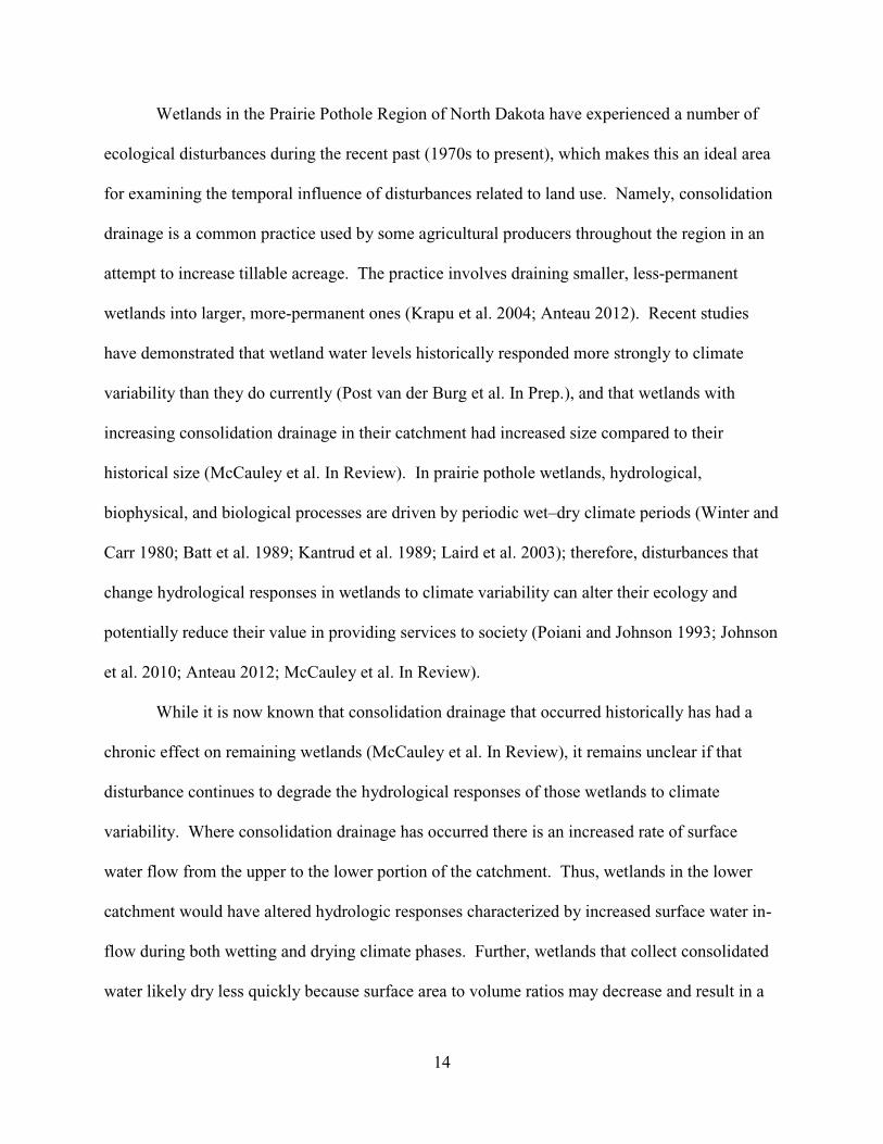
Wetlands in the Prairie Pothole Region of North Dakota have experienced a number of

ecological disturbances during the recent past (1970s to present), which makes this an ideal area

for examining the temporal influence of disturbances related to land use. Namely, consolidation

drainage is a common practice used by some agricultural producers throughout the region in an

attempt to increase tillable acreage. The practice involves draining smaller, less-permanent

wetlands into larger, more-permanent ones (Krapu et al. 2004; Anteau 2012). Recent studies

have demonstrated that wetland water levels historically responded more strongly to climate

variability than they do currently (Post van der Burg et al. In Prep.), and that wetlands with

increasing consolidation drainage in their catchment had increased size compared to their

historical size (McCauley et al. In Review). In prairie pothole wetlands, hydrological,

biophysical, and biological processes are driven by periodic wet–dry climate periods (Winter and

Carr 1980; Batt et al. 1989; Kantrud et al. 1989; Laird et al. 2003); therefore, disturbances that

change hydrological responses in wetlands to climate variability can alter their ecology and

potentially reduce their value in providing services to society (Poiani and Johnson 1993; Johnson

et al. 2010; Anteau 2012; McCauley et al. In Review).

While it is now known that consolidation drainage that occurred historically has had a

chronic effect on remaining wetlands (McCauley et al. In Review), it remains unclear if that

disturbance continues to degrade the hydrological responses of those wetlands to climate

variability. Where consolidation drainage has occurred there is an increased rate of surface

water flow from the upper to the lower portion of the catchment. Thus, wetlands in the lower

catchment would have altered hydrologic responses characterized by increased surface water in-

flow during both wetting and drying climate phases. Further, wetlands that collect consolidated

water likely dry less quickly because surface area to volume ratios may decrease and result in a

15

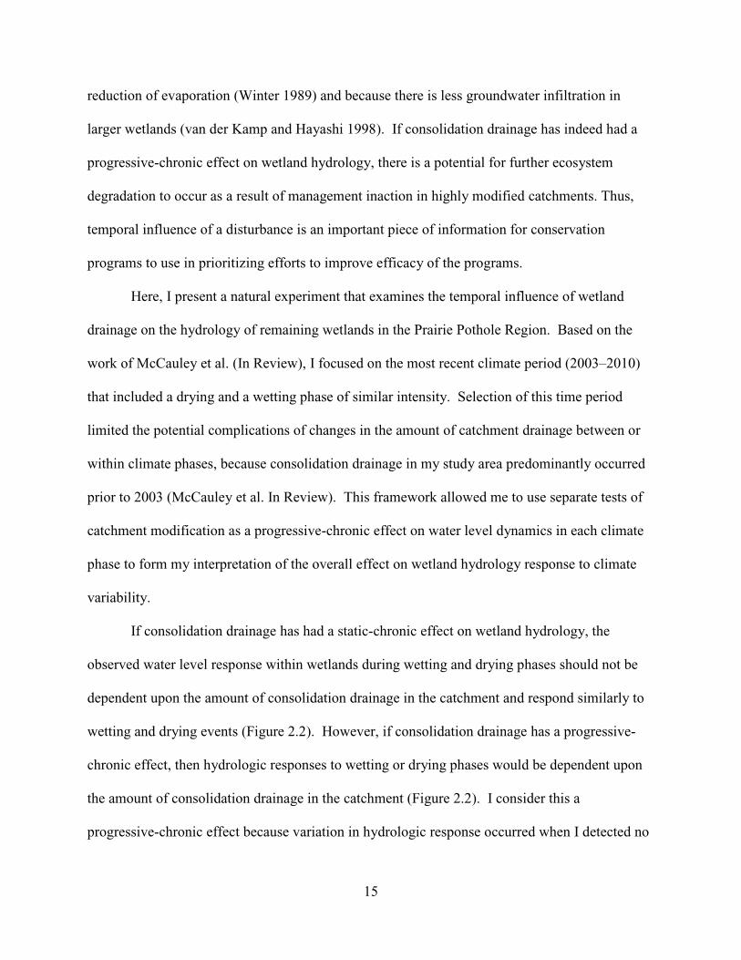
reduction of evaporation (Winter 1989) and because there is less groundwater infiltration in

larger wetlands (van der Kamp and Hayashi 1998). If consolidation drainage has indeed had a

progressive-chronic effect on wetland hydrology, there is a potential for further ecosystem

degradation to occur as a result of management inaction in highly modified catchments. Thus,

temporal influence of a disturbance is an important piece of information for conservation

programs to use in prioritizing efforts to improve efficacy of the programs.

Here, I present a natural experiment that examines the temporal influence of wetland

drainage on the hydrology of remaining wetlands in the Prairie Pothole Region. Based on the

work of McCauley et al. (In Review), I focused on the most recent climate period (2003–2010)

that included a drying and a wetting phase of similar intensity. Selection of this time period

limited the potential complications of changes in the amount of catchment drainage between or

within climate phases, because consolidation drainage in my study area predominantly occurred

prior to 2003 (McCauley et al. In Review). This framework allowed me to use separate tests of

catchment modification as a progressive-chronic effect on water level dynamics in each climate

phase to form my interpretation of the overall effect on wetland hydrology response to climate

variability.

If consolidation drainage has had a static-chronic effect on wetland hydrology, the

observed water level response within wetlands during wetting and drying phases should not be

dependent upon the amount of consolidation drainage in the catchment and respond similarly to

wetting and drying events (Figure 2.2). However, if consolidation drainage has a progressive-

chronic effect, then hydrologic responses to wetting or drying phases would be dependent upon

the amount of consolidation drainage in the catchment (Figure 2.2). I consider this a

progressive-chronic effect because variation in hydrologic response occurred when I detected no

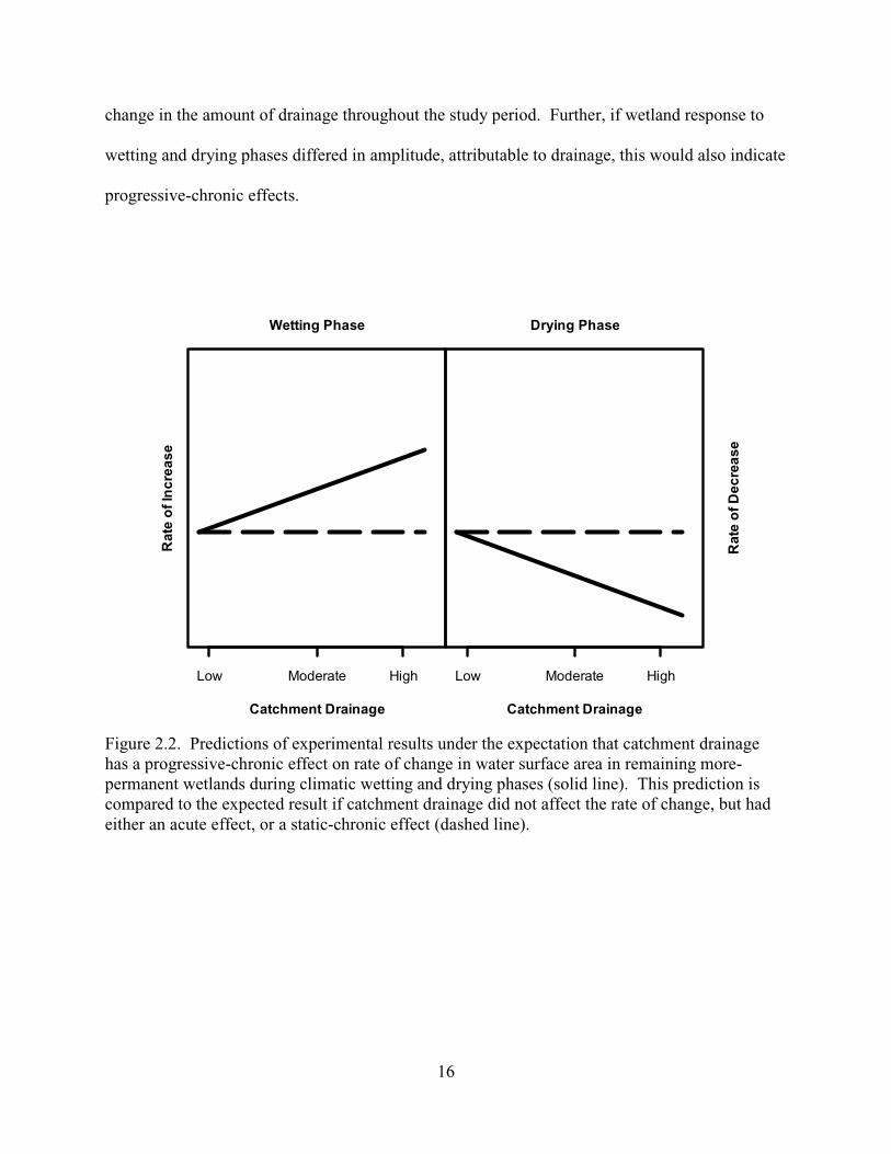
16

change in the amount of drainage throughout the study period. Further, if wetland response to

wetting and drying phases differed in amplitude, attributable to drainage, this would also indicate

progressive-chronic effects.

Figure 2.2. Predictions of experimental results under the expectation that catchment drainage has a progressive-chronic effect on rate of change in water surface area in remaining more-permanent wetlands during climatic wetting and drying phases (solid line). This prediction is compared to the expected result if catchment drainage did not affect the rate of change, but had either an acute effect, or a static-chronic effect (dashed line).

Catchment Drainage

Low Moderate High

Rat

e o

f In

crea

se

Wetting Phase

Catchment Drainage

Low Moderate High

Rat

e o

f Dec

reas

e

Drying Phase

17

Methods

Study Area

My study area was the Prairie Pothole Region of North Dakota (Figure 2.3) where

wetlands of varying water permanence (hereafter, hydroperiods) have formed within glacially-

created depression basins that were historically surrounded by temperate grassland. In these

wetlands, hydrological, biophysical, biological processes are driven by periodic wet–dry periods

caused by an oscillating climate pattern (Winter and Carr 1980; Batt et al. 1989; Kantrud et al.

1989; Laird et al. 2003). Larger and more-permanent wetlands were of particular interest in this

study because their condition is affected by disturbances throughout a larger watershed area that

often includes multiple smaller, less-permanent wetland basins; therefore, larger, more-

permanent wetlands may indicate the condition of the landscape (Anteau and Afton 2011).

Accordingly, I studied lacustrine semipermanent and shallow-water permanent wetlands

(Cowardin et al. 1979) that were originally randomly selected by Anteau and Afton (2008; n =

153) and visited once in 2004 or 2005. Wetlands must have had an open water area larger than

120 m across to be surveyed in 2004 or 2005. In 2004 or 2005, if reselection in the field was

necessary, the nearest suitable semipermanent or permanent wetland was surveyed. In 2010 and

2011, I was able to return to and collect necessary data from 122 of the original 153 wetlands.

Based on National Wetland Inventory classification (NWI; U.S. Fish and Wildlife Service 2003),

67% of wetlands were semipermanent, 3% seasonal, and the rest were permanent wetlands or

shallow-water lakes. Those wetlands classified by NWI as seasonal were reselected wetlands

that were more characteristic of semipermanent wetlands at the time of the field assessment in

2004 or 2005.

18

Figure 2.3. North Dakota study area with Prairie Pothole Region shaded, counties east of the Missouri River outlined, and randomly selected townships outlined wherein three wetlands were randomly sampled. Inset map of the United States and Canada showing the location of the Prairie Pothole Region (shaded) and North Dakota (bold outline).

Data Preparation

Climate index

I used a fine-scale climatic wetland hydrologic index (2.5 arc-minute) derived by Post

van der Burg et al. (In Prep.) to estimate the effect of climate on water surface area within

wetlands using the standardized precipitation-evapotranspiration index (SPEI; Vicente-Serrano et

al. 2010) calculated from PRISM (Parameter-elevation Regression on Independent Slopes

Model) Climate Group data (PRISM Climate Group 2002; Di Luzio et al. 2008). SPEI can

summarize moisture surpluses or deficits by aggregating the difference between precipitation and

potential evaporation over different time scales. During the period of my study, uniformly

averaged monthly climate conditions over the previous six years best explained wetland water

19

levels (Post van der Burg et al. In Prep.). Index values above zero represent wetter climate

conditions and values below zero represent drier conditions.

Based on climate conditions, I designated 2003–2005 as a wet period, 2006–2008 as a

dry period, and 2009–2010 as a wet period. I then identified the drying phase as the change

between the first wet period and the dry period, and the wetting phase as the change between the

dry period and the second wet period. I structured my analysis of wetland surface area change

by these two climate phases. In North Dakota, there is geographic variability in 1) the amount of

variability in the difference between precipitation and evapotranspiration, and 2) the intensity of

wetting and drying phases during one period of time (Laird et al. 2003; Post van der Burg et al.

In Prep.). In my model, I controlled for the influence of geographic variability in the intensity of

wetting and drying phases by using the peak-to-peak amplitude of the climatic wetland

hydrologic index for each phase.

Catchments

I used wetland catchments defined by McCauley et al. (In Review) that were delineated

using high-resolution digital elevation models (DEM) to detect the portion of the landscape

where surface water flows into the focal wetland. These catchments were an index of watershed

derived wetland complexes that included more-intermittent wetlands and their catchments

(McCauley and Anteau 2014). DEM source data included 1 m pixel lidar (data available from

the U.S. Geological Survey) or ~1.25 m pixel interferometric synthetic aperture radar (IfSAR;

Intermap Technologies, Inc., Englewood, Colorado). I used catchment size in my analysis, but I

also used the extent of the catchment to define the area to assess land use effects upon wetlands

(McCauley and Anteau 2014). For logistical reasons associated with assembling landscape

variables, such as amount of wetland area drained, I used catchments truncated to a 2.5 km

20

maximum radius from the wetland basin for 46% of catchments because they were large or

highly irregular in shape. The 2.5-km radius encompassed >90% of the total catchment area for

68% of catchments. Landscape conditions within these 2.5-km truncated catchments should

represent the condition of the full catchment, and the conditions nearest the wetland basin likely

influence the basin most. Therefore, I assume the 2.5-km-truncated catchment provided a

reasonable area to evaluate impacts of land use in this system and are an improvement over the

simply buffering around a wetland a set distance, a common practice (McCauley and Anteau

2014).

Catchment drainage

I used estimates of the percent of the catchment area that was drained wetland during

2003–2010 from multiple data sources, including: aerial photographs, DEM, NWI, and spatially

explicit soil data (see McCauley et al. In Review). Wetlands were identified as drained if they

were present in historical photographs (dating back to 1937) but not present in current

photographs, or if the wetlands were identified as part of a drainage network. Significant

drainage occurred prior to 2003 in my study area; however, I found negligible evidence of

additional drainage after 2003.

Basin area

Within a catchment, I defined the basin as the topographic depression that collects

surface water and which is isolated from basins of other wetlands of an equal or more permanent

hydroperiod. I calculated the maximum potential water surface area of each basin using the

high-resolution DEMs (3 m pixel lidar or 5 m pixel IfSAR) to find the elevation at which water

flows out of the basin (i.e., spill point) and then delineated the area at that spill point elevation

within the basin. Because I predicted that wetlands in basins that were near full or that were full

21

would have less surface area dynamics, I calculated the proportion of the basin that the focal

wetland filled at the start of each climate phase. I used a logit transformation of the proportion-

basin-full variable × 0.1 for use in my analysis.

Water surface area

I delineated water surface area for each surveyed wetland by photointerpretation of

National Agriculture Imagery Program (NAIP; U.S. Department of Agriculture) aerial imagery

for 2003–2006 and 2009–2010 (McCauley et al. In Review). Photointerpretation was performed

while images were viewed as panchromatic instead of true-color, because they were done as part

of a larger study that involved panchromatic imagery (see McCauley et al. In Review). Where

the waterline was obscured by emergent vegetation, the waterline was approximated to be

halfway between the emergent-vegetation to open-water interface and clearly identifiable upland.

NAIP imagery was not available for 2007 and 2008. For those years I used wetland water

surface area delineated once in either 2007 or 2008 using high-resolution digital elevation model

(DEM; source data: 1 m pixel lidar; Data available from the U.S. Geological Survey) or ~1.25 m

pixel interferometric synthetic aperture radar (IfSAR) orthorectified image (Intermap

Technologies, Inc., Englewood, Colorado).

I calculated the rate of increase in water surface area for each wetland during each

climate phase as the natural logarithm of the quotient of final surface area divided by the initial

surface area. For this calculation I used the maximum surface area from the wet period and the

minimum surface area from the dry period. The rate of increase was useful as a response

variable in my model because it allowed me to evaluate temporal dynamics, in a way that is

similar to that used in population biology (Hastings 1997).

22

Maximum depth

Depth of a wetland, along with topography (see Bank Slope below), can be used to

describe wetland basin shape and how water volume is distributed within the basin. To account

for the relationship of surface area and depth, I measured water depth (±0.1 m) at four locations

in each wetland. Locations were along randomly selected transects at 60 m from the shoreline or

emergent vegetation ring toward the center of the wetland. I used the maximum observation

from the initial survey in 2004 or 2005 in my analysis.

Bank slope

I calculated the bank slope of each wetland because I expected water-volume-to-surface

area relationships to differ with varying bank slopes. Wetlands with steeper sides would have

smaller changes in surface area with added volume than wetlands with flatter sides. I recorded

the average elevation of the water surface for all wetlands in 2007 or 2008 (the driest years) and

in 2010 (a wet year) using high-resolution DEMs. I calculated the average radius of each

wetland polygon in 2007 or 2008 and 2010 using surface area calculations of each wetland

(radius = �area/π ). I calculated bank slope as change in water surface elevation from 2010 to

2007 or 2008 divided by the change in radius from 2010 to 2007 or 2008. On average, 2010 was

a wetter year and water levels were higher than in 2007 or 2008 but in those rare cases (~5%)

where 2010 water levels were actually lower than in 2007 or 2008, another wetter year was

substituted.

Land use

I indexed current agricultural impacts within the catchment by calculating the proportion

of the upland that was cropland (i.e. row crop or small grains). Each quarter-quarter section (~16

ha) within the catchment was classified as cropland if ≥50% of the upland area was determined

23

to be cropped from photointerpretation of 2003 or 2004 NAIP imagery (see McCauley et al. In

Review).

Statistical Analyses

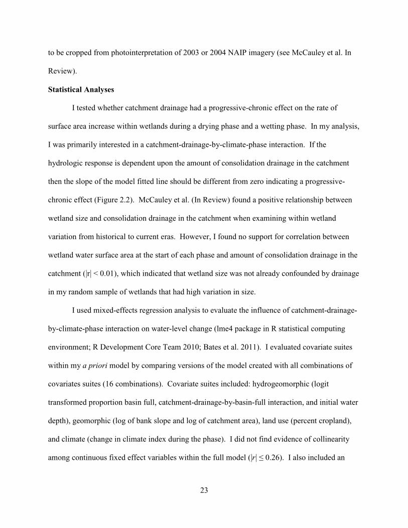
I tested whether catchment drainage had a progressive-chronic effect on the rate of

surface area increase within wetlands during a drying phase and a wetting phase. In my analysis,

I was primarily interested in a catchment-drainage-by-climate-phase interaction. If the

hydrologic response is dependent upon the amount of consolidation drainage in the catchment

then the slope of the model fitted line should be different from zero indicating a progressive-

chronic effect (Figure 2.2). McCauley et al. (In Review) found a positive relationship between

wetland size and consolidation drainage in the catchment when examining within wetland

variation from historical to current eras. However, I found no support for correlation between

wetland water surface area at the start of each phase and amount of consolidation drainage in the

catchment (|r| < 0.01), which indicated that wetland size was not already confounded by drainage

in my random sample of wetlands that had high variation in size.

I used mixed-effects regression analysis to evaluate the influence of catchment-drainage-

by-climate-phase interaction on water-level change (lme4 package in R statistical computing

environment; R Development Core Team 2010; Bates et al. 2011). I evaluated covariate suites

within my a priori model by comparing versions of the model created with all combinations of

covariates suites (16 combinations). Covariate suites included: hydrogeomorphic (logit

transformed proportion basin full, catchment-drainage-by-basin-full interaction, and initial water

depth), geomorphic (log of bank slope and log of catchment area), land use (percent cropland),

and climate (change in climate index during the phase). I did not find evidence of collinearity

among continuous fixed effect variables within the full model (|r| ≤ 0.26). I also included an

24

interaction of each covariate by climate phase because I expected the rate of increase to be of

opposite sign between climate phases. I identified wetland as a random error term to account for

the repeated measure across climate phase and to ensure proper variance estimates for fixed

effects of all models. I interpreted and made predictions from the most parsimonious

combination of covariate suites, which I evaluated by the number of estimated parameters and

Akaike’s Information Criterion adjusted for small sample size (AICc; Burnham and Anderson

2002). I evaluated model goodness-of-fit using the squared correlation coefficient (r2) between

observations and model fitted values. Confidence intervals for fixed effect estimates were

calculated at the 85% level to best match criteria used during covariate suite selection using

AICC (Arnold 2010).

I plotted the effect of catchment drainage on the rate of increase during the wetting phase

and rate of decrease (rate of increase × –1) for the drying phase separately for three levels of

basin full. I sliced the basin full variable at the 25th, 50th, and 75th percentiles, representing less

full, moderately full, and near full, respectively. I plotted the predicted effect of catchment

drainage on rate of change (increase or decrease, appropriately) for wetlands for a spectrum of

percent basin full to illustrate the degree of net balance in water budgets through drying and

wetting phases. For the drying phase I plotted effect estimates for 3–90% of basin full,

representing the 1st to 75th percentile of my data, because this range represents wetlands that

would likely remain isolated from downstream surface water connections throughout the drying

phase. For the wetting phase I plotted effect estimates for 1–34% of basin full, representing the

1st to 25th percentile of my data, because these wetlands remained below the spill point

throughout the wetting phase; therefore, the estimates were not influenced by water spilling out

of the basin. Additional covariates were set to median values in all effect plots.

25

Results

My analysis included a total of 122 wetlands of which catchment sizes ranged from 4–

200,900 ha and the mean was 3,686 ha (median = 394 ha). Percent of catchment area that was

drained wetland ranged from 0–13% (median = 1.1%). Basin area ranged from 1.7–6,646 ha and

the mean was 182 ha (median = 34 ha). On average, at the start of the drying period basins were

67% full (SD = 27, 25th percentile = 51% full, median = 67% full, 75th percentile = 90% full) and

at the start of the wetting period basins were 53% full (SD = 27, 25th percentile = 34% full,

median = 50% full, 75th percentile = 73% full). Percent of upland that was cropland averaged

52% and ranged from 0–100% (median = 55%). The mean wetland water surface area was 65.4

ha (SD = 129. 8, median = 24.5 ha) during the two wet periods and 54.7 ha (SD = 118.2, median

= 17.4 ha) during the dry period. My climate index ranged from -1.6 to 2.0. Mean climate index

for each period was different from zero in the expected direction for the climate period (Figure

2.4). The mean differences in climate index were -0.83 (SE = 0.03) and 0.89 (SE = 0.04) during

the drying and wetting phases, respectively.

My final model of wetland surface area dynamics included the treatment effect of

catchment-drainage-by-climate-phase interaction, hydrogeomorphic and climate covariate suites,

and the random error term (Table 2.1). My model explained 52%, 13%, and 51% of the

variability within the observations overall, within the drying phase, and within the wetting phase,

respectively. Model parameter estimates are reported in Table 2.2. Catchment drainage when

focal wetland basins were less full was positively correlated with rate of increase in water

surface area during the wetting phase and negatively correlated with rate of decrease in water

surface area during the drying phase (Figure 2.5A). Catchment drainage was not correlated with

rate of water surface area change during either the drying or wetting phase where focal wetlands

26

moderately filled their basin (Figure 2.5B). Catchment drainage when focal wetland basins were

nearly full was negatively correlated with rate of increase in water surface area during the

wetting phase and positively correlated with rate of decrease in water surface area during the

drying phase (Figure 2.5C). The rate of change in wetland surface area became increasingly

different between the drying and wetting phases with increased catchment drainage (Figure 2.6).

Discussion

My results indicate that past wetland drainage in a catchment can have a progressive-

chronic effect on drying and wetting phases of remaining wetlands and potentially on overall

wetland hydrology throughout the Prairie Pothole Region. This effect appears to manifest itself

in an unbalancing of wetland water budgets, which culminates in a pattern of increasing wetland

size over consecutive wet–dry climate fluctuations. This result indicates that the full impact of

historical wetland drainage has not yet been realized and that further degradation of wetland

ecosystems is likely because catchment drainage appears to influence succession of remaining

wetlands toward lake-like hydroperiods, as wetlands grow to and maintain at their spill point

elevations. This finding is a significant piece of information that could inform decisions about

wetland restoration, because inaction will lead to further degradation of semipermanent wetland

ecosystems. Here, I propose a mechanism by which to explain previously observed trends that

indicate an increase in the size of wetlands compared to historical size within drained catchments

(McCauley et al. In Review).

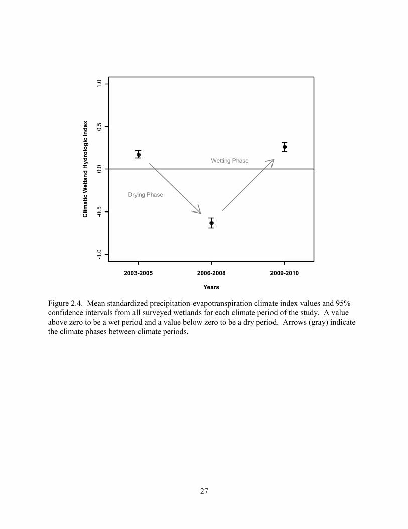
27

Figure 2.4. Mean standardized precipitation-evapotranspiration climate index values and 95% confidence intervals from all surveyed wetlands for each climate period of the study. A value above zero to be a wet period and a value below zero to be a dry period. Arrows (gray) indicate the climate phases between climate periods.

Years

Clim

atic

Wet

lan

d H

ydro

log

ic In

dex

2003-2005 2006-2008 2009-2010

-1.0

-0.5

0.0

0.5

1.0

Drying Phase

Wetting Phase

28

Table 2.1. Covariate suite selection results from an a priori model used to examine the effect of catchment drainage on water-level dynamics in wetlands of North Dakota during a drying and a wetting phase, included are: model log likelihood (LL), number of estimated parameters (K), Akaike’s Information Criterion for small sample size (AICC), increase over lowest AICC (∆AICC), and Akaike model weight (wi) for combinations of covariate suites (wi ≥0.01).

Covariate Suites LL K AICC ∆AICC wi

Hydrogeomorphic, Climate -118.78 13 265.15 0.00 0.45

Hydrogeomorphic, Land Use, Climate

-116.76 15 265.64 0.49 0.35

Hydrogeomorphic -122.70 11 268.55 3.40 0.08

Hydrogeomorphic, Land Use

-120.51 13 268.59 3.44 0.08

Hydrogeomorphic, Geomorphic, Land Use

-117.56 17 271.83 6.68 0.02

All Covariate Suites -115.44 19 272.27 7.12 0.01

No Covariate Suites -166.54 6 345.43 80.28 0.00

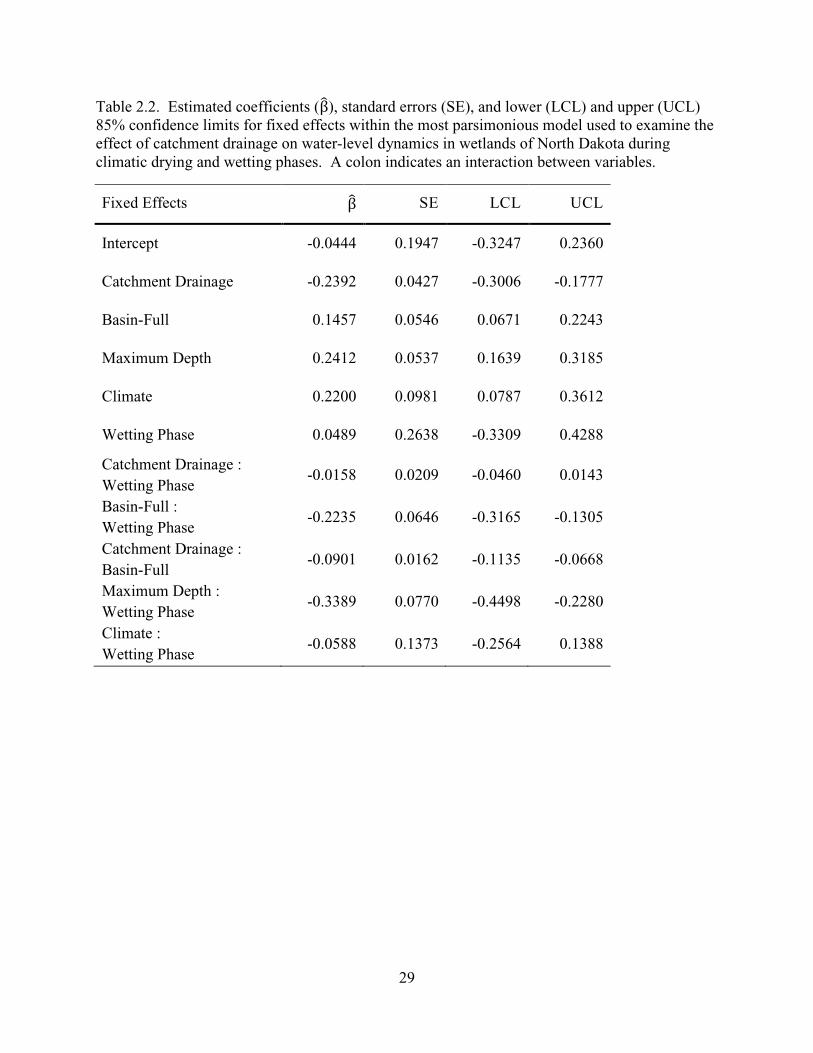
29

Table 2.2. Estimated coefficients (β�), standard errors (SE), and lower (LCL) and upper (UCL) 85% confidence limits for fixed effects within the most parsimonious model used to examine the effect of catchment drainage on water-level dynamics in wetlands of North Dakota during climatic drying and wetting phases. A colon indicates an interaction between variables.

Fixed Effects β� SE LCL UCL

Intercept -0.0444 0.1947 -0.3247 0.2360

Catchment Drainage -0.2392 0.0427 -0.3006 -0.1777

Basin-Full 0.1457 0.0546 0.0671 0.2243

Maximum Depth 0.2412 0.0537 0.1639 0.3185

Climate 0.2200 0.0981 0.0787 0.3612

Wetting Phase 0.0489 0.2638 -0.3309 0.4288

Catchment Drainage : Wetting Phase

-0.0158 0.0209 -0.0460 0.0143

Basin-Full : Wetting Phase

-0.2235 0.0646 -0.3165 -0.1305

Catchment Drainage : Basin-Full

-0.0901 0.0162 -0.1135 -0.0668

Maximum Depth : Wetting Phase

-0.3389 0.0770 -0.4498 -0.2280

Climate : Wetting Phase

-0.0588 0.1373 -0.2564 0.1388

30

Figure 2.5. Model predicted effects of past wetland drainage on the rates of increase and decrease in wetland water surface area (85% confidence intervals) derived from observations of semipermanent and permanent wetlands in North Dakota during a recently wet–dry climate fluctuation. Predictions were made for focal wetlands that were (A) less full, (B) moderately full, and (C) almost full, determined by 25th, 50th, and 75th percentiles of the data for the drying phase (51%, 67%, and 90%), and for wetting phase (34%, 50%, and 73%), respectively. Solid lines represent estimates with a slope different from zero and dashed lines represent estimates with a slope not different than zero.

Rat

e o

f In

crea

se

0.0

0.5

1.0 A Less full basin

Wetting Phase

0.0

0.5

1.0

Drying Phase

Rat

e o

f Dec

reas

e

Rat

e o

f In

crea

se

0.0

0.5

1.0 B Moderately full basin

0.0

0.5

1.0

Rat

e o

f Dec

reas

e

Rat

e o

f In

crea

se

0 3 6 9 12

0.0

0.5

1.0 C Near full basin

% Catchment Drainage0 3 6 9 12

0.0

0.5

1.0

Rat

e o

f Dec

reas

e

% Catchment Drainage

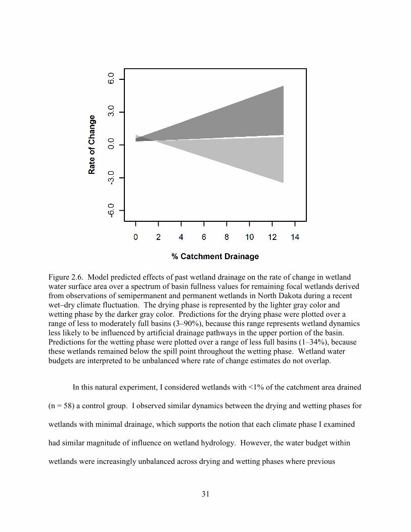
31

Figure 2.6. Model predicted effects of past wetland drainage on the rate of change in wetland water surface area over a spectrum of basin fullness values for remaining focal wetlands derived from observations of semipermanent and permanent wetlands in North Dakota during a recent wet–dry climate fluctuation. The drying phase is represented by the lighter gray color and wetting phase by the darker gray color. Predictions for the drying phase were plotted over a range of less to moderately full basins (3–90%), because this range represents wetland dynamics less likely to be influenced by artificial drainage pathways in the upper portion of the basin. Predictions for the wetting phase were plotted over a range of less full basins (1–34%), because these wetlands remained below the spill point throughout the wetting phase. Wetland water budgets are interpreted to be unbalanced where rate of change estimates do not overlap.

In this natural experiment, I considered wetlands with <1% of the catchment area drained

(n = 58) a control group. I observed similar dynamics between the drying and wetting phases for

wetlands with minimal drainage, which supports the notion that each climate phase I examined

had similar magnitude of influence on wetland hydrology. However, the water budget within

wetlands were increasingly unbalanced across drying and wetting phases where previous

32

drainage in catchments was >2% of area. I suspect that wetlands receiving consolidation

drainage water from historical drainage efforts will continue to increase in size with each

subsequent wetting phase, until they reach their spill point and then stabilize. This effect is most

evident in wetlands that have not yet filled to their natural or artificial spill point. Whereas, in

wetlands that were more full the rate of increase in water surface area decreased during the

wetting phase and the rate of decrease in water surface area increased during the drying phase,

likely due to water spilling out of the basin through either the natural or artificial spill points.

My observations support the hypothesis that consolidation of wetlands leads to semipermanent

and permanent wetlands in drained catchments experiencing a successional change toward a

more lake-like condition which likely has regional-scale implications on both the integrity of

wetland ecosystems and social benefits derived from services provided by wetlands (Anteau

2012).

This natural experiment demonstrates a case where legacy effects on ecosystems can

continue to degrade the integrity of an ecosystem after a disturbance activity has ceased and that

lack of management action likely will result in further deterioration of ecosystem function.

Identification of historical drainage of wetlands within the catchment of remaining wetlands

could inform the prioritization of conservation efforts to initially focus on remediation of

wetlands that have not yet reach their basin spill points, and restoring complexes of less-

permanent wetlands in the upper catchment to improve surface water reduction through natural

processes (Weller 1988; Galatowitsch and van der Valk 1994; Knutsen and Euliss 2001). Such

restoration would then likely restore more natural water-level dynamics within wetlands lower in

the catchment and improve hydrologic processes that maintain ecological integrity of wetland

systems and provide services to society (Anteau 2012). This case study also demonstrates the

33

importance of 1) re-evaluating previous studies that initially evaluated the condition of an

ecosystem before and after a disturbance, because the full effect of the disturbance may continue

beyond the temporal scale of the initial study, or 2) structuring analyses to evaluate the rate of

environmental change in relation to either historical rate or to a contemporaneous rate of a

complementary ecosystem process. In my case, comparing wetting and drying rates as

complementary processes in wetlands within modified catchments versus unmodified catchments

allowed me to evaluate long-term effects of consolidation drainage and infer the overall effect on

balance of wetland water budgets.

Agricultural intensity has increased in the Prairie Pothole Region since the 1800s,

generally following a southeast to northwestern pattern (Samson and Knopf 1994). As such,

there has been a varying period of catchment modification (Dahl 1990). In a recent evaluation of

productivity in more-permanent wetlands within the region, productivity appeared to be

decreased overall and showed a spatial pattern of stronger declines in the southeast compared to

the northwest (Anteau and Afton 2011). My results suggest one potential mechanism for that

loss of productivity was the progressive-chronic effect of consolidation drainage, as wetlands in

landscapes that have been modified for longer have had more time to reach their spill points and

stabilize. In North Dakota, I found 39% of more-permanent wetlands had sufficient drainage

within their catchments to unbalance their water budget and 23% of those wetlands to have filled

>90% of their maximum area. The remainder of the wetlands in drained catchments likely will

reach spill-over levels if management actions are not taken, but if the frequency or intensity of

wetting phases increases due to climate change this process likely would be accelerated. At

either rate, increased wetland size and reduced water-level fluctuation may result in a decline in

productivity similar to those observed in Iowa and Minnesota (Anteau and Afton 2011).

34

My findings also corroborate the idea that drainage of less-permanent wetlands has led to

greater amounts of water consolidated into fewer basins and those basins tend to be larger and

more stable than they were historically (Krapu et al. 2004; Anteau 2012; McCauley et al. In

Review). Consolidation drainage networks essentially speed the flow of surface water thereby

reducing infiltration into groundwater (Winter 2003). Furthermore, more inputs into a wetland

tends to reduce the surface area to volume ratio, which greatly reduces evapotranspiration

(Winter 1989). Together, these mechanisms suggest that consolidation of water inhibits the

natural processes that would reduce surface water within a catchment (LaBaugh et al. 1987;

Winter and Rosenberry 1995; Winter 2003). Consequently, more surface water is stored in

larger wetlands and when those wetlands reach spill-over levels more surface water flows out of

the catchments into larger watersheds. Accordingly, consolidation drainage can convert non-

contributing catchments into contributing catchments of larger watersheds, thus becoming

conducive to downstream flooding.

Increased wetland size and stabilized water levels can have deleterious effects on the

integrity of wetland ecosystems and the services they historically provided. As wetlands

increase in size they flood new habitat that provides nutrients to drive wetland productivity

through decomposition of vegetation and flooding of nutrient-rich soils. However, in modified

catchments once wetland water levels reach basin spill point elevations, water levels are likely to

become stabilized. Stabilization of water levels could reduce availability of nutrients in the

system, because during sustained lake phases nutrients get tied up in anoxic sediments.

Historically, these would become available again if the wetland draws down and sediments

oxidize (Euliss et al. 1999). Stabilized water levels also might drive a change in ecological

community structure because species more adapted to stable conditions become dominant where

35

there is a lack of water fluctuation (Van der Valk and Davis 1980). For example, Typha spp.

proliferate in stable water environments (Swanson 1992; Shay et al. 1999; Boers and Zedler

2008); and, higher, more stable water levels allow fish populations to become established in

wetlands where they were previously controlled by inhabitable conditions during drawdown

periods (Peterka 1989; Anteau and Afton 2008; Herwig et al. 2010).

Prairie pothole wetlands are an important resource for migratory waterbirds during spring

and fall migration and during the breeding season. Many waterbirds use these wetlands as

stopover sites where they rely on invertebrates to meet energy requirements of long migration

flights, and for building energy and nutrient supplies for breeding in the region or in other areas

on the continent (Batt et al. 1989; Swanson and Duebbert 1989; Anteau and Afton 2006, 2011).

Consequently, stabilization of water levels after chronic increases in water level is a concern for

waterbird conservation because of the likely decreases in wetland productivity. Indeed, drainage

of less-permanent wetlands and stabilization of water levels in more-permanent wetlands may

already be affecting waterbird populations (Niemuth et al. 2006; Anteau and Afton 2011;

McCauley & Anteau unpublished manuscript) and potentially other native inhabitants of these

wetlands, such as amphibians (Balas et al. 2012; Herwig et al. 2013; Mushet et al. 2014).

Consolidation drainage has been implicated in water-level increases in wetlands that

receive drainage water (Anteau 2012; McCauley et al. In Review), and my results suggest that

past drainage causes chronic flooding effects. As more-permanent wetlands continue to increase

in area, surrounding uplands are at higher risk for being flooded. Further, remaining wetlands

that reach their spill point have reduced or no ability to provide flood protection and flood waters

may then cascade into larger-scale watershed flooding problems. My findings suggest that once

these basins fill, catchments surrounding those basins transition from a non-contributing to

36

contributing area of larger order watersheds. Thus, landscapes within the Prairie Pothole Region

are shifting from catchments that may be only intermittently connected at the surface to larger-

order watersheds with much more hydrologic connectivity. While I think it is likely this shift is

occurring wherever there is consolidation drainage, there are opportunities to test this hypothesis

in larger watersheds of North Dakota (e.g., Devils Lake, Red River of the North, or Missouri

River) that have recently experienced flooding of increased intensity and magnitude. Using

techniques such as those outlined by McCauley and Anteau (2014), more detailed study of

formerly isolated catchments that are now contributing to larger watersheds could provide more

accurate information regarding the impact of wetland drainage on flooding within these larger

watersheds. This question deserves thorough investigation because the reduction in flood control

that wetlands can provide due to consolidation drainage has probably had a great economic cost,

and those costs will continue to come in the form of inundated property, damaged infrastructure,

and new flood control infrastructure lower in the watershed.

Progressive-chronic effects of anthropogenic modifications to the environment are likely

present throughout other systems. For example, installation of dams on river systems likely has

a static-chronic effect on flows if water management is consistent, but those dams may have a

progressive-chronic effect on sediment accumulation in reservoirs and river-bed incision.

Anthropogenically induced environmental change continues to alter services that ecosystems

provide to society, while reducing the integrity of the ecosystem, which likely will result in

permanent ecosystem change. There is a fundamental difference between managing the

cumulative harmful effects of continued anthropogenic disturbance to ecosystems, and

identifying and managing legacy effects of past disturbances that continue to degrade

ecosystems. Fortunately, identifying the positive feedback mechanisms within ecosystems that

37

were initiated by historical disturbances could help land managers improve their ability to

develop management strategies to counteract these disturbances on managed ecosystems.

Literature Cited



Anteau, M. J., and A. D. Afton. 2006. Diet shifts of lesser scaup are consistent with the spring

condition hypothesis. Canadian Journal of Zoology 84:779–786.





Arnold, T. W. 2010. Uninformative parameters and model selection using Akaike's information

criterion. Journal of Wildlife Management 74:1175–1178.

Balas, C., N. Euliss, Jr., and D. Mushet. 2012. Influence of conservation programs on

amphibians using seasonal wetlands in the Prairie Pothole Region. Wetlands 32:333–345.

Bates, D., M. Maechler, and B. Bolker. 2011. lme4: Linear mixed-effects models using S4

classes. R package version 0.999375-42. http://CRAN.R-project.org/package=lme4/




Boers, A. M., and J. B. Zedler. 2008. Stabilized water levels and Typha invasiveness. Wetlands

28:676–685.

38

Burnham, K. P., and D. R. Anderson. 2002. Model Selection and Multimodel Inference: A

Practical Information-Theoretic Approach, Second Edition ed. Springer-Verlag, New

York, NY, USA.

Cowardin, L. M., V. Carter, F. C. Golet, and E. T. LaRoe. 1979. Classification of Wetlands and

Deepwater Habitats of the United States. U. S. Department of the Interior, Fish and

Wildlife Service, Washington, D.C., USA. FWS/OBS 79/31, 131 p.

Cuddington, K. 2011. Legacy effects: the persistent impact of ecological interactions. Biological

Theory 6:203–210.



Di Luzio, M., G. L. Johnson, C. Daly, J. K. Eischeid, and J. G. Arnold. 2008. Constructing

retrospective gridded daily precipitation and temperature datasets for the conterminous

United States. Journal of Applied Meteorology and Climatology 47:475–497.





514.

Foster, D., F. Swanson, J. Aber, I. Burke, N. Brokaw, D. Tilman, and A. Knapp. 2003. The

importance of land-use legacies to ecology and conservation. Bioscience 53:77–88.

Galatowitsch, S. M., and A. G. van der Valk. 1994. Restoring Prairie Wetlands: An Ecological

Approach. Iowa State University Press, Ames, IA, 246 p.

39

Harding, J. S., E. F. Benfield, P. V. Bolstad, G. S. Helfman, and E. B. D. Jones. 1998. Stream

biodiversity: the ghost of land use past. Proceedings of the National Academy of Sciences

95:14843–14847.

Hastings, A. 1997. Population Biology: Concepts and Models. Springer, New York, NY, USA.

Herwig, B. R., L. W. Schroeder, K. D. Zimmer, M. A. Hanson, D. F. Staples, R. G. Wright, and

J. A. Younk. 2013. Fish Influences on amphibian presence and abundance in prairie and

parkland landscapes of Minnesota, USA. Journal of Herpetology 47:489–497.

Herwig, B. R., K. D. Zimmer, M. A. Hanson, M. L. Konsti, J. A. Younk, R. W. Wright, S. R.

Vaughn, and M. D. Haustein. 2010. Factors influencing fish distributions in shallow lakes

in prairie and prairie-parkland regions of Minnesota, USA. Wetlands 30:609–619.

Holling, C. S. 1973. Resilience and stability of ecological systems. Annual Review of Ecology

and Systematics 4:1–23.

Johnson, W. C., B. Werner, G. R. Guntenspergen, R. A. Voldseth, B. Millett, D. E. Naugle, M.

Tulbure, R. W. H. Carroll, J. Tracy, and C. Olawsky. 2010. Prairie wetland complexes as

landscape functional units in a changing climate. Bioscience 60:128–140.




Knutsen, G. A., and N. H. Euliss, Jr. 2001. Wetland Restoration in the Prairie Pothole Region of

North America: A Literature Review. U. S. Department of the Interior, Geological

Survey, Reston, VA, USA. Biological Science Report USGS/BRD/BSR—2001-0006,

54 p.

40




LaBaugh, J. W., T. C. Winter, V. A. Adomaitis, and G. A. Swanson. 1987. Hydrology and

Chemistry of Selected Prairie Wetlands in the Cottonwood Lake Area, Stutsman County,

North Dakota, 1979–82. U. S. Department of the Interior, Geological Survey,

Washington, D.C., USA. Professional Paper 1431 1431, 26 p.

Laird, K. R., B. F. Cumming, S. Wunsam, J. A. Rusak, R. J. Oglesby, S. C. Fritz, and P. R.

Leavitt. 2003. Lake sediments record large-scale shifts in moisture regimes across the

northern prairies of North America during the past two millennia. Proceedings of the

National Academy of Sciences 100:2483–2488.

Martin, S. L., D. B. Hayes, D. T. Rutledge, and D. W. Hyndman. 2011. The land-use legacy

effect: adding temporal context to lake chemistry. Limnology and Oceanography

56:2361–2370.



McCauley, L. A., and M. J. Anteau. 2014. Generating nested wetland catchments with readily-

available digital elevation data may improve evaluations of land-use change on wetlands.

Wetlands 34:1123–1132.

Mushet, D. M., J. L. Neau, and N. H. Euliss Jr. 2014. Modeling effects of conservation grassland

losses on amphibian habitat. Biological Conservation 174:93–100.

41

Niemuth, N., M. Estey, R. Reynolds, C. Loesch, and W. Meeks. 2006. Use of wetlands by

spring-migrant shorebirds in agricultural landscapes of North Dakota’s Drift Prairie.




Poiani, K. A., and W. C. Johnson. 1993. Potential effects of climate change on a semi-permanent

prairie wetland. Climatic Change 24:213–232.

Post van der Burg, M., M. J. Anteau, L. A. McCauley, and M. T. Wiltermuth. In Prep. Making

climate indices relevant to wetland hydrology.

PRISM Climate Group. 2002. Parameter-elevation regressions on independent slopes model.

Oregon State University.

R Development Core Team. 2010. R: A language and environment for statistical computing. R

Foundation for Statistical Computing, Vienna, Austria. http://www.R-project.org/

Samson, F., and F. Knopf. 1994. Prairie conservation in North America. Bioscience 44:418–421.

Scheffer, M., S. R. Carpenter, J. A. Foley, C. Folke, and B. Walker. 2001. Catastrophic shifts in

ecosystems. Nature 413:591–596.



19:413–425.

Spaling, H., and B. Smit. 1995. A conceptual model of cumulative environmental effects of

agricultural land drainage. Agriculture, Ecosystems and Environment 53:99–108.

42

Sterling, P., and J. Eyer. 1988. Allostasis: a new paradigm to explain arousal pathology. In S.

Fisher, and J. T. Reason (eds) Handbook of Life Stress, Cognition, and Health. Wiley,

Chicester, NY, USA.




Swanson, G. A., and H. F. Duebbert. 1989. Wetland habitats of waterfowl in the Prairie Pothole

Region. In A. G. van der Valk (ed) Northern Prairie Wetlands. Iowa State University

Press, Ames, IA, USA, pp 228–267.

Turner II, B. L., R. E. Kasperson, W. B. Meyer, K. M. Dow, D. Golding, J. X. Kasperson, R. C.

Mitchell, and S. J. Ratick. 1990. Two types of global environmental change: definitional

and spatial-scale issues in their human dimensions. Global Environmental Change 1:14–

22.

U.S. Fish and Wildlife Service. 2003. National Wetlands Inventory.

http://www.fws.gov/wetlands/.

van der Kamp, G., and M. Hayashi. 1998. The groundwater recharge function of small wetlands

in the semi-arid northern prairies. Great Plains Research 8:39–56.

Van der Valk, A. G., and C. B. Davis. 1980. The impact of a natural drawdown on the growth of

four emergent species in a prairie glacial marsh. Aquatic Botany 9:301–322.

Vicente-Serrano, S. M., S. Beguería, and J. I. López-Moreno. 2010. A multiscalar drought index

sensitive to global warming: the Standardized Precipitation Evapotranspiration Index.

Journal of Climate 23:1696–1718.

43

Weller, M. 1988. Issues and approaches in assessing cumulative impacts on waterbird habitat in

wetlands. Environmental Management 12:695–701.

Winter, T., and D. Rosenberry. 1995. The interaction of ground water with prairie pothole

wetlands in the Cottonwood Lake area, east-central North Dakota, 1979–1990. Wetlands

15:193–211.

Winter, T. C. 1989. Hydrologic studies of wetlands in the northern prairie. In A. G. van der Valk

(ed) Northern Prairie Wetlands. Iowa State University Press, Ames, IA, USA, pp 16–54.

Winter, T. C. 2003. Hydrological, Chemical, and Biological Characteristics of a Prairie Pothole

Wetland Complex Under Highly Variable Climate Conditions: The Cottonwood Lake

Area, East-central North Dakota. U. S. Department of the Interior, Geological Survey,


Winter, T. C., and M. R. Carr. 1980. Hydrologic Setting of Wetlands in the Cottonwood Lake

Area, Stutsman County, North Dakota. U. S. Department of the Interior, Geological

Survey, Denver, CO, USA. Water-Resources Investigation Report 80-99, 42 p.

44

CHAPTER 3. IS CONSOLIDATION DRAINAGE AN INDIRECT MECHANISM FOR

INCREASED ABUNDANCE OF CATTAIL IN NORTHERN PRAIRIE WETLANDS?

Abstract

Plant communities are structured by environmental conditions and the variability in those

conditions. Within northern prairie wetlands these conditions are primarily driven by water

levels and water chemistry. Therefore, disturbances to wetlands or their catchments that disrupt

water-level fluctuations in response to wet–dry climatic periods have the potential to alter natural

vegetative communities in favor of species that proliferate in stable environments, such as cattail

(Typha spp.). I evaluated the effect of water-level dynamics during a recent wet–dry climate

fluctuation on cattail coverage within wetlands situated in catchments with varying land use and

amounts of wetland drainage. I found that water depth increased more where wetlands filled less

of their topographic basin (β� = -0.006 ± 0.002 SE), had steeper bank slopes (β� = 0.124 ± 0.042

SE), and were in larger catchments (β� = 0.069 ± 0.032 SE). Proportion of the wetland covered

by cattail was negatively correlated with increased water depth (β� = -0.090 ± 0.027 SE), bank

slope (β� = -0.067 ± 0.013 SE) and wetland area (β� = -0.039 ± 0.013 SE). Existing evidence

suggests that drainage of wetlands within catchments of remaining wetlands causes water levels

to progressively increase until the topographic basin fills and then water levels stabilize. Thus,

the eventual filling and stabilizing of wetlands caused by consolidation drainage offers a

potential mechanism for increased cattail coverage observed on the northern prairie landscape.

Increased cattail coverage within a wetland reduces the quality of the wetland to support diverse

plant, invertebrate, and waterbird communities.

45

Introduction

It has been suggested that the prevalence of monotypic stands of cattail (Typha spp.) has

increased for prairie wetlands (Kantrud 1992; Swanson 1992; Anteau and Afton 2008), which

has implications for abundance and quality of food resources and foraging habitat for waterbirds,

particularly shorebirds. When shallow-water zones become dominated by cattails, wetlands have

less shallow-water foraging habitat, a reduction in or absence of submerged aquatic vegetation,

and a reduction in the variety of decomposer organisms—including macroinvertebrates that are

important food resources for waterbirds (Voigts 1976; Kantrud 1986). Monotypic stands of

cattails within wetlands may eliminate foraging and roosting habitat needed by migrating and

breeding shorebirds and waterfowl (Weller and Spatcher 1965; Voigts 1976; Kantrud 1986;

Anteau 2012). Landscape modifications likely have altered natural wetland hydrology that

included water-level fluctuation, changed sedimentation and nutrification, or introduced species

within wetlands (Galatowitsch et al. 2000; Gleason et al. 2003; Anteau 2012). Such changes

might be responsible for greater cattail abundance and resultant degradation of many wetland

ecosystems across North America (Galatowitsch et al. 1999). Therefore, it is important to

understand how landscape modifications have influenced the abundance of cattails and the

concomitant value of those wetlands to waterbirds to inform ongoing conservation efforts to

reverse the trend of increasing cattail encroachment in wetlands of the Prairie Pothole Region.

Hydrologic fluctuations in response to climate variability help shape floral community

structure of prairie wetlands. While plant community composition shifts in response to wet–dry

climate periods, the overall community structure is dominated by floral species adapted to

dynamic hydrologic conditions (Stewart and Kantrud 1972; Grace and Wetzel 1981; LaBaugh et

al. 1987; Kantrud et al. 1989; van der Valk 2005). Higher and more-stable water regimes may

46

shift emergent communities toward cattail-dominated systems because cattails proliferate in

more-stable environments (Swanson 1992; Shay et al. 1999; Boers and Zedler 2008).

Disturbances within wetlands and their surrounding catchment that increase

sedimentation and nutrient loading into wetlands or stabilize water levels may create conditions

more favorable to cattail invasions in prairie pothole wetlands (Wang et al. 1994; Gleason and

Euliss 1998; Shay et al. 1999). Increased sedimentation can decrease wetland depth through

addition of nutrient-rich soil while reducing or eliminating competing wetland plant species

(Jurik et al. 1994; Gleason and Euliss 1998). These conditions favor development of monotypic

stands of cattail (Gleason and Euliss 1998; Galatowitsch et al. 1999; Shay et al. 1999). Further,

additional nitrogen inputs from uplands can promote growth and expansion of cattail, especially

where nitrogen is limiting (Shay et al. 1999). Moreover, stabilization of water levels can

increase soil release of phosphorus and increase uptake by cattail resulting in enhanced growth

(Boers and Zedler 2008). Nutrient enrichment of wetlands with high and stable water-levels can

lead to changes in vegetation structure and consequently changes in the macroinvertebrate

community (Voigts 1976; McCormick et al. 2004) because species that are best adapted to

exploit available nutrients will gain a competitive advantage over those adapted for a more

oligotrophic environment.

In the Prairie Pothole Region of North Dakota, cattail was previously found during 2002

to be present in 28% of wetlands and averaged 37% areal coverage within wetlands that

contained cattail (Ralston et al. 2007). It is likely that monotypic stands of cattail will continue

to increase in occurrence and coverage within wetlands where hydrology has been modified and

uplands disturbed (Kantrud 1992; Swanson 1992; Anteau and Afton 2008); therefore, there is a

need to quantitatively evaluate factors that may be contributing to wetland conditions that are

47

favorable to increased cattail coverage. Accordingly, I examined the influence of hydrologic and

land-use factors on coverage of cattail within semipermanent and permanent wetlands. I

expected cattail coverage to be greater within wetlands where water levels were more stable and

where agricultural land-use modified uplands with drainage networks and tillage.

Methods

Study Area

I returned to wetlands within the Prairie Pothole Region of North Dakota (Figure 3.1) that

were previously randomly selected and surveyed once in 2004 or 2005 (hereafter, 2004/05) by

Anteau and Afton (2008; n = 153). Wetlands were randomly selected within a hierarchal

sampling design of three regions, three sub-regions, clusters of three townships, and three

wetlands within each township (Anteau and Afton 2008). Accordingly, I included township as a

random error term to account for this clustered design. These were lacustrine semipermanent

and shallow-water permanent wetlands (Cowardin et al. 1979) that must have had an open-water

area larger than 120 m across to be surveyed in 2004/05. In 2004/05, if reselection in the field

was necessary, the nearest suitable semipermanent wetland was surveyed. In April and May of

2011, I returned to 126 of the original 153 wetlands. Based on the National Wetland Inventory

classification (NWI; U.S. Fish and Wildlife Service 2003), 67% of wetlands surveyed were

semipermanent, 3% seasonal, and the rest were permanent wetlands or shallow-water lakes.

Those wetlands classified by NWI as seasonal were wetlands reselected in the field in 2004/05

that were more characteristic of semipermanent wetlands at time of field assessment.

My selection of wetlands was not completely random in regards to cattail coverage

within semipermanent and permanent wetlands throughout the region. My selection was

confined to more-permanent wetlands that had at least 120 m of open water to address objectives

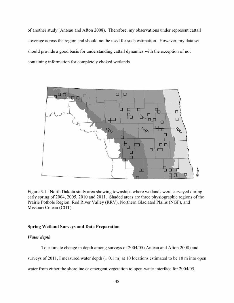
48

of another study (Anteau and Afton 2008). Therefore, my observations under represent cattail

coverage across the region and should not be used for such estimation. However, my data set

should provide a good basis for understanding cattail dynamics with the exception of not

containing information for completely choked wetlands.

Figure 3.1. North Dakota study area showing townships where wetlands were surveyed during early spring of 2004, 2005, 2010 and 2011. Shaded areas are three physiographic regions of the Prairie Pothole Region: Red River Valley (RRV), Northern Glaciated Plains (NGP), and Missouri Coteau (COT).

Spring Wetland Surveys and Data Preparation

Water depth

To estimate change in depth among surveys of 2004/05 (Anteau and Afton 2008) and

surveys of 2011, I measured water depth (± 0.1 m) at 10 locations estimated to be 10 m into open

water from either the shoreline or emergent vegetation to open-water interface for 2004/05.

49

When waves were present, I recorded the average depth between wave crests and troughs. Prior

to field work, I delineated the shoreline or emergent vegetation to open-water interface of each

wetland using imagery (National Agricultural Imagery Program, U.S. Department of

Agriculture; hereafter NAIP) acquired in the summer (July) prior to each spring survey

conducted by Anteau and Afton (2008). I used the imagery from the previous year because it

better represents the location of the emergent vegetation to open-water interface that Anteau and

Afton (2008) used to locate their sampling locations. I digitized the interface by using a

geographic information system (GIS) at a scale of 1:5,000. I offset (i.e. buffered) the digitized

open-water interface by 10 m in the direction of the wetland center to approximate locations of

2004/05 sampling. I derived my 10 random points from the 10-m buffer, but I constrained point

locations so there is a minimum distance of 40 m between points. I navigated to survey locations

that were pre-loaded onto a GIS data logger (Trimble GeoXT, Trimble Navigation, Sunnyvale,

CA). Survey locations found within the emergent vegetation ring were recorded as such,

because different dynamics of sedimentation and accumulation of organics were expected.

Emergent vegetation

I estimated the width of emergent vegetation coverage (0, 1–4, 5–10, 11–30, 31–60, or

>60 m) and the proportion (± 0.1) of emergent vegetation that was cattail at 10 randomly

selected transects that extended perpendicular from the shoreline through the random points

where water depth measurements were taken to the center of the wetland. I calculated an

average width of cattail coverage for each wetland using the midpoint value of the 10 categorical

estimates of emergent vegetation coverage (maximum value of 90 m) multiplied by the

proportion that was cattail. Finally, I calculated the area of cattail coverage within each wetland

50

by using a GIS to create a polygon from the perimeter of the wetland measured using 2010

imagery (see below) extending inward the distance of the average width of cattail coverage.

Land use

I classified current agricultural impacts immediately surrounding each wetland using

ground observations in 2011. I used GIS software in the field to attributed empty polygon

outlines of land-cover data (Habitat and Population Evaluation Team 1996) based on current

observations with one of the following categories: native grassland, restored grassland, unknown

grassland, hayland, cropland, shrubs, trees, developed, barren, or wetland. I calculated the

proportion of cropland for the upland area that was both within the defined catchment (see

below) and within 400 m of the subject wetland. I also estimated the width of upland grass

buffer (0, 1-4, 5-10, 11-50, >50 m) between any development or agricultural land use and the

wetland. In my analyses I used the midpoint of categorical estimates, with maximum value of

75 m.

Water surface area

I used water surface area delineated for each surveyed wetland by McCauley et al. (In

Review) using photointerpretation of NAIP aerial imagery for 2003–2006 and 2009–2010.

Photointerpretation was performed while images were viewed as panchromatic instead of true-

color, because they were done as part of a larger study that involved some panchromatic imagery

(see McCauley et al. In Review). Where the waterline was obscured by emergent vegetation, the

waterline was approximated to be halfway between the emergent-vegetation to open-water

interface and clearly identifiable upland. NAIP imagery was not available for 2007 and 2008.

For those years I used wetland water surface area delineated once in either 2007 or 2008 using

high-resolution digital elevation model (DEM; source data: 1 m pixel lidar; Data available from

51

the U.S. Geological Survey) or ~1.25 m pixel interferometric synthetic aperture radar (IfSAR)

orthorectified image (Intermap Technologies, Inc., Englewood, Colorado).

Catchments

I used wetland catchments as an index of watershed derived wetland complexes defined

as the portion of the landscape in which surface water flows into a focal wetland, and included

more-intermittent wetlands and their catchments (McCauley and Anteau 2014; McCauley et al.

In Review). Catchments were derived for each of the surveyed wetlands using high resolution

DEMs (3 m pixel lidar or 5 m pixel IfSAR) and surface hydrology modeling tools (McCauley

and Anteau 2014; McCauley et al. In Review). Some catchments (46%) that were large or

highly irregular in shape were truncated to a 2.5 km maximum radius from the wetland basin for

logistical reasons associated with assembling landscape variables, such as amount of wetland

area drained. The 2.5-km radius encompassed >90% of the total catchment area for 68% of

catchments. Landscape conditions within these 2.5-km truncated catchments should represent

the condition of the full catchment, and the conditions nearest the wetland basin likely influence

the basin most. Therefore, I assumed the 2.5-km-truncated catchment provided a reasonable area

to evaluate impacts of land use in our system and are an improvement over the simply buffering

around a wetland a set distance, a common practice (McCauley and Anteau 2014).

Catchment drainage

I used estimates of the percent catchment area that was drained wetland during 2003–

2010 using multiple data sources, including: aerial photographs, DEM, NWI, and spatially

explicit soil data (McCauley et al. In Review). Wetlands were identified as drained if they were

present in historical photographs (dating back to 1937) but not present in current photographs, or

if the wetlands were identified as part of a drainage network. Significant drainage occurred prior

52

to 2003 in our study area; however, there was negligible evidence of additional drainage after

2003.

I also recorded presence of drainage networks and connections between wetlands while in

the field in 2011. Surface-water connections include: inflow and outflow streams, ditches,

culverts, and temporal connections between wetland basins.

Basin area

I defined a wetland basin as the topographic depression that collects surface water that

which is isolated from basins of other wetlands of an equal or more permanent hydroperiod. I

measured the basin area to determine the maximum water surface area of a wetland that the basin

could hold before the water would spill and flow out of the basin. I used the high-resolution

DEMs (3 m pixel lidar or 5 m pixel IfSAR) to find the spill point of the basin and then delineated

the area at that spill point elevation within the basin. Because wetlands in basins that were near

full or that were full would have less surface area dynamics (Chapter 2), I calculated the

proportion of the basin that the focal wetland filled at the start of each climate phase.

Climate

I used a fine-scale climate index (2.5 arc-minute) derived by Post van der Burg et al. (In

Prep.) to estimate the spatially-explicit effect of climate on increase in water depth of wetlands.

The climate index used a standardized precipitation-evapotranspiration index calculated from

PRISM (Parameter-elevation Regression on Independent Slopes Model) Climate Group data

(PRISM Climate Group 2002). The temporal summary of the index that best explained water

levels in the current era, and used here, incorporated climate conditions over the previous six

years with a uniform average across years (Post van der Burg et al. In Prep.). For each wetland, I

53

calculated the difference in climate index values from the wet period during 2003–2005 and wet

period in 2009–2010.


Water depth increase

I examined the potential influence of climate, upland disturbance and wetland

connectivity on increased in wetland depth from 2004/05 to 2011 using mixed-effects regression

analysis (Package lme4 in R Statistical Computing Environment; R Development Core Team

2010; Bates et al. 2011). I created an a priori full model that included independent variables

including: difference in climate index, percent catchment area that was drained wetland,

presence/absence of wetland surface connections, percent surrounding upland that was cropland,

basin full percent, natural logarithm of bank slope, and natural logarithm of catchment area. I

also included interaction terms for difference in climate index-by-catchment area because

climate variability likely has a greater influence on water depth of wetlands in smaller

catchments than on larger catchments, and for wetland drainage-by-basin full percent because

water depth within wetlands that already filled their basins would be less influenced by drainage

within the catchment than would wetlands that have potential for increased water depth. I found

no evidence of strong correlations among dependent variables within the full model (|r| ≤ 0.24).

I evaluated variables in my a priori full model by comparing a one-variable-removed

reduced model to the full model (Arnold 2010). I assumed the removed variable was informative

if the Akaike’s Information Criterion adjusted for small sample size (AICc; Burnham and

Anderson 2002) of the reduced model was increased ≥2 points; all informative variables were

compiled into a final reduced model. I first evaluated each two-way interaction relative to the

full model and removed any interactions not supported from the full model before conducting the

54

variable selection process for all main effect variables. I specified township as a random error

term. I compared the final model to a null model using AICC to determine model adequacy

(Burnham and Anderson 2002). I evaluated the variation captured by the model from

interpretation of the squared correlation coefficient from the observed and fitted values.

Cattail coverage

I evaluated how coverage of cattail within wetlands in 2011 may have been influenced by

the change in water depth from 2004/05 to 2011, rate of water surface area change during a

drying phase 2003–2005 to 2006–2008, wetland drainage within the catchment, and amount of

upland that is cropland using a mixed effect regression analysis (Package lme4 in R Statistical

Computing Environment; R Development Core Team 2010; Bates et al. 2011). In my a priori

full model I also included the natural logarithm of wetland area, percent of the topographic basin

filled by the wetland, natural logarithm of bank slope as independent variables, and I included a

cropland-by-upland buffer width interaction term because a grass upland buffer can mitigate the

effects of surrounding land use on wetland quality (Anteau and Afton 2008; Anteau et al. 2011).

I found no evidence of strong correlations among independent variables within the a priori full

model (|r| ≤ 0.25), with the exception of cropland and upland buffer (r = -0.65) for which the

interaction term was included. I evaluated independent variables in the full model and created a

reduced model using the variable selection method described above. I specified township as a

random error term, compared the final model to a null model using AICC to determine model

adequacy (Burnham and Anderson 2002), and evaluated the variation captured by the model

from the squared correlation coefficient of the observed and fitted values. I plotted model

predicted effects across the observed range of variable of interest and held other variables at

median levels. I used 85% confidence intervals for interpretation of importance for variables to

55

be more consistent with the threshold used during variable selection within the full model using

AICC (Arnold 2010).

Results

Within the 126 wetlands visited in early spring of 2011 average water surface area was

68 ha (median = 26 ha, range = 1–965 ha, SD = 132) in July of 2010. Maximum water depth

within wetlands in spring 2011 averaged 2.0 m (SD = 0.7), and on average, wetland water depth

increased 1.1 m (SE = 0.1) from 2004/05 to 2011 (Figure 3.2). We detected cattail on at least

one transect at 51% of wetlands.

My final model used to explain increased water depth contained independent variables

including: percent basin full, bank slope, catchment area, and difference in climate index (Table

3.1). This model explained 54% of the variation in water depth increase and was 16 AICC points

better than a null model and held all of the Akaike model selection weight (wi). Water depth

increased more where wetlands filled less of their topographic basin, had steeper bank slopes,

and were in larger catchments (Table 3.2). Increase in wetland depth also occurred where

climate index indicated wetter conditions (Table 3.2).

My final model used to explain cattail coverage within wetlands contained independent

variables including: increase in water depth, bank slope, and wetland area (Table 3.3). This

model explained 38% of the variation in cattail coverage among wetlands and was better than a

null model (∆AICC = 43, wi = 0). Proportion of wetlands covered by cattail was negatively

correlated with increased water depth (β� = -0.090 ±0.027 SE; Figure 3.3). Cattail coverage was

also negatively correlated with bank slope (β� = -0.067 ±0.013 SE) and wetland area (β� = -0.039

±0.013 SE).

56

Figure 3.2. Histogram showing increased water depth within 126 more-permanent wetlands in North Dakota from 2004 or 2005 to 2011.

Increase in Depth (m)

Per

cen

t of W

etla

nd

s

0

5

10

15

0 1 2 3

57

Table 3.1. Reduction of independent variables from an a priori full model used to examine the effect of wetland setting and climate on water depth increase in more-permanent wetlands from 2004 or 2005 to 2011 in North Dakota. Changes in model log likelihood (∆LL), number of estimated parameters (∆K), and Akaike’s Information Criterion for small sample size (∆AICC) are reported for the model with that variable removed relative to the referenced full model. We deemed covariates important (IMP) if their removal causes a >2 ∆K increase in AICC. A colon indicates an interaction between variables.

Variable Removed ∆LL ∆K ∆AICc IMP

Climate : Catchment Area a -0.9 -1 -0.6 No

Drainage : Basin-Full a -0.1 -1 -2.2 No

Basin-Full b -4.1 -1 5.8 Yes

Bank Slope b -3.5 -1 4.7 Yes

Climate b -3.3 -1 4.3 Yes

Catchment Area b -2.4 -1 2.4 Yes

Cropland b -0.4 -1 -1.5 No

Surface Connection b -0.2 -1 -2.0 No

Drainage b 0.0 -1 -2.4 No

a Compared to full model: LL = -122.2, K = 12, AICC = 271.2 b Compared to model with no interactions: LL = -123.2, K = 10, AICC = 268.3

58

Table 3.2. Estimated coefficients (β�), standard errors (SE), and 85% lower (LCL) and upper (UCL) confidence limits for fixed effects within the final reduced model used to examine the effect of wetland setting and climate on water depth increase in more-permanent wetlands from 2004 or 2005 to 2011 in North Dakota.


Intercept 1.4544 0.3046 1.0159 1.8930

Basin-Filled -0.0063 0.0022 -0.0094 -0.0032

Bank Slope 0.1243 0.0419 0.0640 0.1847

Catchment Area 0.0687 0.0315 0.0233 0.1140

Climate 0.3062 0.1234 0.1285 0.4839

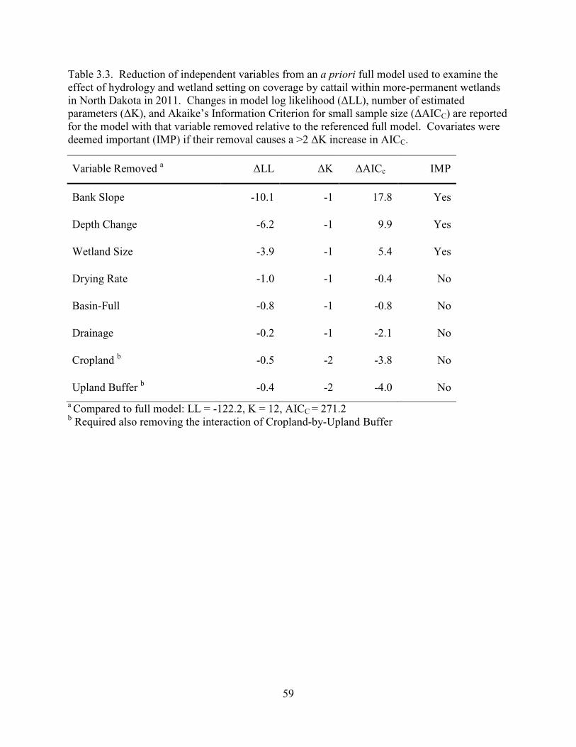
59

Table 3.3. Reduction of independent variables from an a priori full model used to examine the effect of hydrology and wetland setting on coverage by cattail within more-permanent wetlands in North Dakota in 2011. Changes in model log likelihood (∆LL), number of estimated parameters (∆K), and Akaike’s Information Criterion for small sample size (∆AICC) are reported for the model with that variable removed relative to the referenced full model. Covariates were deemed important (IMP) if their removal causes a >2 ∆K increase in AICC.

Variable Removed a ∆LL ∆K ∆AICc IMP

Bank Slope -10.1 -1 17.8 Yes

Depth Change -6.2 -1 9.9 Yes

Wetland Size -3.9 -1 5.4 Yes

Drying Rate -1.0 -1 -0.4 No

Basin-Full -0.8 -1 -0.8 No

Drainage -0.2 -1 -2.1 No

Cropland b -0.5 -2 -3.8 No

Upland Buffer b -0.4 -2 -4.0 No

a Compared to full model: LL = -122.2, K = 12, AICC = 271.2 b Required also removing the interaction of Cropland-by-Upland Buffer

60

Figure 3.3. Model estimated effect (85% CI) of increase in water depth on cattail coverage within more-permanent wetlands in North Dakota.

Discussion

My results show that wetland water depth was greater during the recent wetting phase

than that at the end of the previous wet period. However, increases in water depth were limited

within wetlands that had already filled, or nearly filled to their topographic basin. Additionally, I

observed a strong correlation between increased water depth and less cattail coverage, suggesting

Increase in Depth (m)

Cat

tail

cove

rag

e (p

rop

ort

ion

wet

lan

d a

rea)

0 1 2 3

-0.2

-0.1

0.0

0.1

0.2

0.3

0.4

61

cattail was eliminated where water depth increased. This process of cattail elimination by

flooding during wet periods is consistent with observations from other studies (Weller and

Spatcher 1965; van der Valk 1994). When combined with evidence that drainage of wetlands

within catchments of remaining wetlands causes water levels to progressively increase with each

wet–dry climate period until wetlands fill their topographic basin and then water levels stabilize

(Chapter 2), cattail coverage is kept in check by increases in water level resulting from

consolidation drainage, but ultimately will increase once water levels stabilize at their basin spill

elevation.

Cattail seed germination during drawdown and growth during re-flooding is part of the

natural vegetative cycle in prairie pothole wetlands (Weller and Spatcher 1965; van der Valk and

Davis 1978). Wetlands that experience flooding and drawdown of equal amplitude should

exhibit these natural vegetative cycles. However, when hydrologic responses to climate

variability are disrupted by disturbances within the wetland systems, then vegetative cycles are

also likely to be disrupted resulting in monotypic stands of cattail (Van der Valk and Davis

1980). For example, where consolidation drainage has resulted in higher and more-stable water

levels in remaining wetlands, cattail can become established at the fringes of high water levels.

Cattail is not likely to be eliminated by flooding within wetlands that have filled their

topographic basin because these wetlands have reached their spill-point at which they contribute

to larger watersheds with additional inflow. However, expansion of cattail toward the center of

the wetland can occur by extension of the habitable zone as a result of sedimentation and

accretion of organic debris (Waters and Shay 1992; Gleason and Euliss 1998; Shay et al. 1999).

Accumulation of sediment and organic debris increases the rate of habitable zone expansion,

ultimately reducing the water depth required to reach the basin spill point elevation. Wetlands in

62

landscapes with high agricultural land use are likely to have greater rates of sedimentation and

nutrient input (Gleason and Euliss 1998), than those surrounded by grasslands, making those

wetlands prime environments for cattail.

Consolidation drainage appears to have more of an indirect effect on increased cattail

coverage in wetlands through altered water-level fluctuations, rather than a direct effect.

Consolidation drainage actually could keep cattail coverage low in wetlands that have not yet

filled their topographic basin, because as a result of each climatic wetting phase water levels

progressively increase (Chapter 2) to flood existing cattail stands. However, that is only a

temporary response, until a wetland basin is full and water levels stabilize. Once water-levels

stabilized, cattail coverage is likely to increase within wetlands where consolidation drainage has

occurred.

My observations provide evidence that landscape modifications that have altered

hydrologic processes within wetlands have the potential to alter natural vegetative cycles,

resulting in increased coverage of cattail in monotypic stands rather than more diverse plant

communities interspersed within wetlands. This change can negatively impact invertebrate

forage and waterbird populations that feed on aquatic invertebrates. Restoration of more natural

water-level fluctuations in response to wet–dry climate periods, perhaps through restoration of

complexes of wetlands with vary hydroperiods, may restore vegetative cycles and transition

monotypic stands of cattail back into vegetative communities that vary in wetland coverage

according to hydrologic conditions.

Literature Cited



63






Arnold, T. W. 2010. Uninformative parameters and model selection using Akaike's information

criterion. Journal of Wildlife Management 74:1175–1178.



Boers, A. M., and J. B. Zedler. 2008. Stabilized water levels and Typha invasiveness. Wetlands

28:676–685.



York, NY, USA.




Galatowitsch, S., D. Whited, R. Lehtinen, J. Husveth, and K. Schik. 2000. The vegetation of wet

meadows in relation to their land-use. Environmental Monitoring and Assessment

60:121–144.

Galatowitsch, S. M., N. O. Anderson, and P. D. Ascher. 1999. Invasiveness in wetland plants in

temperate North America. Wetlands 19:733–755.

64

Gleason, R., N. Euliss, D. Hubbard, and W. Duffy. 2003. Effects of sediment load on emergence

of aquatic invertebrates and plants from wetland soil egg and seed banks. Wetlands

23:26–34.

Gleason, R. A., and N. H. Euliss, Jr. 1998. Sedimentation of prairie wetlands. Great Plains

Research 8:97–112.

Grace, J. B., and R. G. Wetzel. 1981. Habitat partitioning and competitive displacement in

cattails (Typha): experimental field studies. American Naturalist 118:463–474.

Habitat and Population Evaluation Team. 1996. U.S. Fish and Wildlife Service 1996 landcover:

U.S. Fish and Wildlife Service, Bismarck, ND.

Jurik, T. W., S.-C. Wang, and A. G. van der Valk. 1994. Effects of sediment load on seedling

emergence from wetland seed banks. Wetlands 14:159–165.

Kantrud, H. A. 1986. Effects of vegetation manipulation on breeding waterfowl in prairie

wetlands—a literature review. U. S. Department of the Interior, Washington, D.C. Fish

and Wildlife Technical Report 3, 15 p.

Kantrud, H. A. 1992. History of cattails on the prairies: wildlife impacts. In G. M. Linz (ed)

Proceedings of the Cattail Management Symposium. Fargo, ND, USA, pp 9–12

http://www.npwrc.usgs.gov/resource/plants/cattail/kantrud.htm - accessed:1/23/2011.




65









Wetlands 34:1123–1132.

McCormick, P. V., R. B. E. Shuford, and P. S. Rawlik. 2004. Changes in macroinvertebrate

community structure and function along a phosphorus gradient in the Florida Everglades.




PRISM Climate Group. 2002. Parameter-elevation regressions on independent slopes model.

Oregon State University.



Ralston, S. T., G. M. Linz, W. J. Bleier, and H. J. Homan. 2007. Cattail distribution and

abundance in North Dakota. Journal of Aquatic Plant Management 45:21–24.



19:413–425.

66

Stewart, R. E., and H. A. Kantrud. 1972. Vegetation of prairie potholes in North Dakota, in

relation to quality of water and other environmental factors. U. S. Department of the

Interior, Geological Survey, Washington, D.C., USA. Professional Paper 585-D.






van der Valk, A. G. 1994. Effects of prolonged flooding on the distribution and biomass of

emergent species along a freshwater wetland coenocline. Vegetatio 110:185–196.

van der Valk, A. G. 2005. Water-level fluctuations in North American prairie wetlands.


van der Valk, A. G., and C. B. Davis. 1978. The role of seed bands in the vegetation dynamics of

prairie glacial marshes. Ecology 59:322–335.

Van der Valk, A. G., and C. B. Davis. 1980. The impact of a natural drawdown on the growth of

four emergent species in a prairie glacial marsh. Aquatic Botany 9:301–322.

Voigts, D. K. 1976. Aquatic invertebrate abundance in relation to changing marsh vegetation.

American Midland Naturalist 95:313–322.

Wang, S.-C., T. W. Jurik, and A. G. van der Valk. 1994. Effects of sediment load on various

stages in the life and death of cattail (Typha × glauca). Wetlands 14:166–173.

Waters, I., and J. M. Shay. 1992. Effect of water depth on population parameters of a Typha

glauca stand. Canadian Journal of Botany 70:349–351.

67

Weller, M. W., and C. S. Spatcher. 1965. Role of habitat in the distribution and abundance of

marsh birds. Iowa Agriculture and Home Economics Experiment Station, Special Report

43. Ames, Iowa, USA.

68

CHAPTER 4. ALTERED WETLAND HYDROLOGY SUPPORTS INCREASED

PRESENCE OF FISH IN PRAIRIE POTHOLE WETLANDS ACROSS NORTH

DAKOTA

Abstract

In prairie wetlands fish have been implicated in the degradation of habitat for aquatic

invertebrates and in turn for waterbirds. Historically, fish occurrence had been mostly low,

approximately 10–20%, and intermittent in semipermanent and permanent wetlands within the

Prairie Pothole Region due to their depth, chemical and hydrological dynamics, and isolation.

However, landscape modifications such as consolidation drainage of wetlands have increased

water levels, connectivity, and hydroperiods of remaining wetlands. I evaluated how these

changes have influenced the occurrence and abundance of fish in prairie wetlands of North

Dakota and how fish have influenced wetland quality, as measured by the amount of submerged

aquatic vegetation, turbidity, and the nature of aquatic invertebrate communities. Fish were

present in 57% of 138 semipermanent and permeant wetlands surveyed in 2011, an increase of

14% compared to surveys conducted in 2004 and 2005. Logistic regression analysis indicated a

higher probability of fish occurrence in wetlands that had greater water depth (β� = 0.625 ±0.319

SE) and greater wetland connectivity by means of more full topographic basins (β� = 0.020

±0.009 SE). Fish abundance was similarly related to water depth (β� = 0.231 ±0.082 SE) and

more full topographic basins (β� = 0.007 ±0.002 SE), indicated by mixed-effect regression

analysis. Fathead minnow abundance was positively correlated with turbidity (β� = 2.735 ±0.709

SE) and negatively correlated with abundance of submerged aquatic vegetation (β� = -0.209

±0.088 SE) and invertebrate biomass (β� = -0.097 ±0.041 SE) in multivariate multiple regression

analysis. These results indicate an indirect negative influence of consolidation drainage on

69

wetlands’ ability to support productive and diverse invertebrate communities and the waterbird

populations that rely on them, through increased fish abundance and turbidity and decreased

abundance of submerged vegetation.

Introduction

Distribution of fish in wetlands in the Prairie Pothole Region is influenced by isolation of

wetland basins, water depth, and water chemistry all of which are dynamic as a result of

fluctuations between wet and dry climate periods (LaBaugh et al. 1987; Kantrud et al. 1989;

Peterka 1989; Euliss et al. 1999; Leibowitz and Vining 2003). However, anthropogenic

modifications to prairie landscapes have been linked to disruptions of water-level fluctuations

and basin isolation (Euliss and Mushet 1996; Merkey 2006; Anteau 2012). Specifically,

consolidation drainage of wetlands in prairie landscapes has led to more-permanent, larger

wetlands that contain more surface connections to other wetlands (McCauley et al. In Review;

Chapter 2). As a result, these modifications may contribute to an increase in the distribution and

abundance of fish in wetlands (Zimmer et al. 2000; Anteau 2012).

Fish populations in most semipermanent prairie wetlands historically have been

intermittent, dependent upon how wet or dry wetlands are in response to climate fluctuations

(Kantrud et al. 1989; Peterka 1989). During wet periods, fish disperse through flooded

connections among semipermanent and permanent wetlands (Kantrud et al. 1989). Flooding of

previously dried areas within these wetlands induces a pulse in invertebrate productivity

providing abundant food that facilitates growth of local fish populations (Euliss et al. 1999;

Hanson et al. 2005). Higher water-levels provide areas of wetlands that are deep enough for

over-winter survival or provide connections to other areas of winter refugia (Zimmer et al.

2001a). However, when water levels recede wetlands become isolated and fish are less likely to

70

survive as hypoxic conditions cause a winterkill or summerkill event (Kantrud et al. 1989;

Peterka 1989).

Changes in wetland hydrology have the potential to influence ecological communities in

prairie wetlands because native communities are the result of a dynamic and surface isolated

system. Higher, more stable water regimes may shift species composition toward a community

with species that are adapted to more stable environments. Further, increased connectivity

among basins would provide colonization corridors and deep-water refugia for fish that rarely

colonized isolated basins (Herwig et al. 2010). Together these conditions are more favorable for

fish that were previously kept in check by hydrologic dynamics and geographic isolation of

wetlands to become invasive and further threaten natural functions of prairie wetlands (Scheffer

et al. 1993; Hanson et al. 2005; Herwig et al. 2010; Anteau et al. 2011).

Compared to historical accounts, the prevalence of fish in prairie wetlands was

apparently increased in 2004 and 2005, during a high-stable-water regime (Anteau and Afton

2008; Anteau et al. 2011). Increases in occurrence and abundance of fish can decrease

abundance of invertebrates in wetlands thereby reducing forage quality and foraging efficiency

for waterbirds (Swanson and Nelson 1970; Cox et al. 1998; Hanson et al. 2005; Anteau and

Afton 2009). High abundance of fish can impact density of macroinvertebrates (e.g., amphipods

and cladocerans) in wetlands directly through predation and indirectly through increased

turbidity, which decreases submerged vegetation habitat for invertebrates, both resulting in a

change in wetland trophic structure (Scheffer et al. 1993; Hanson and Butler 1994; Zimmer et al.

2000; Zimmer et al. 2001b; Anteau et al. 2011). Abundance of fathead minnows (Pimephales

promelas) are of particular interest regarding the quality of a wetland to support waterbirds in the

region because they are tolerant of a wide range of environmental conditions, have a high rate of

71

reproduction, and are large enough to eat macroinvertebrates, yet have also been found to feed

on detritus that may increase turbidity (Held and Peterka 1974; Gale and Buynak 1982; Hanson

and Riggs 1995; Duffy 1998; Herwig and Zimmer 2007).

Here I examined how landscape modifications that have been linked to higher water

levels, altered water-level fluctuations, and increased wetland connectedness (McCauley et al. In

Review; Chapter 2) have influenced occurrence and abundance of fish in semipermanent and

permanent prairie wetlands of North Dakota. I evaluated their influence on occurrence of fish in

2011, with the expectation that fish had a higher probability of occurrence in wetlands within

modified catchments where water depths were greater and wetlands were more connected based

on evidence from previous studies (Herwig et al. 2010; Anteau et al. 2011; Maurer et al. 2014).

Further, I evaluated whether these factors also increased abundance of fish. Lastly, I evaluated

whether abundance of fish had a negative influence on wetland quality measured by the amount

of submerged aquatic vegetation, turbidity, and invertebrate densities and biomass (Hanson and

Butler 1994; Anteau et al. 2011; Maurer et al. 2014). Through these evaluations, I evaluate the

direct effect landscape modifications have on increased fish occurrence and abundance in

wetlands and indirect effect landscape modifications have on wetland community structure and

productivity through altered wetland hydrology and increased fish abundance.

Methods

Study Area

In 2011, I returned to 138 wetlands within the Prairie Pothole Region of North Dakota

(Figure 4.1) that were previously randomly selected and surveyed once in 2004 or 2005

(hereafter, 2004/05) by Anteau and Afton (2008). These were lacustrine semipermanent and

shallow-water permanent wetlands (Cowardin et al. 1979) that must have had an open-water area

72

larger than 120 m across to be included in the sample during 2004/05. In 2004/05, if reselection

in the field was necessary, the nearest suitable semipermanent wetland was surveyed. In 2011, I

returned to the 81 original wetlands and surveyed 57 additional randomly selected wetlands.

Based on National Wetland Inventory classification (NWI; U.S. Fish and Wildlife Service 2003),

93 of wetlands were semipermanent, 5 seasonal, and 40 permanent wetlands or shallow-water

lakes. The wetlands classified by NWI as seasonal were included because they were more

characteristic of a semipermanent wetland at time of field assessment.

Spring Wetland Surveys

In April and May of 2011, I surveyed wetlands using techniques described in Anteau and

Afton (2008) to collect data on fish abundance, invertebrate density, water quality, and wetland

vegetation structure. I collected data on randomly located transects extending from shoreline

toward the center of the wetland. I recorded data electronically and georeferenced all sampling

locations at the time of collection with a geographic information system (GIS) data logger

(Trimble GeoXT, Trimble Navigation, Sunnyvale, CA).

Fish communities

I used minnow traps and an experimental gill net in wetlands to determine relative

abundance of fish (Anteau and Afton 2008). I set five Gee-style minnow traps with 6.35-mm

mesh at the emergent vegetation to open-water interface (or equivalent position from the

shoreline if no emergent vegetation is present) at five transects. I set the monofilament

experimental gill net (21 × 2 m with seven 3-m panels ranging in mesh size from 1.9–7.6 cm) at

one of the five transects, positioned perpendicular to the shoreline with the small mesh end of the

net at the emergent vegetation to open-water interface (or equivalent position from the shoreline

if no emergent vegetation was present). Minnow traps and the gill net were deployed for 12–24

73

hours including an overnight period. At the time of trap and gill net retrieval, I sorted and

counted fish by species and by length category (<5, 5–10, 10–20, 20–40, >40 cm).

Figure 4.1. North Dakota study area showing townships where wetlands were surveyed during early spring of 2004, 2005, and 2011. Counties are outlined within the shaded region representing the Prairie Pothole Region.

I classified fish captures into one of three categories: fathead minnows, other small fish

species typically <10 cm (e.g., other minnows [Cyprinidae], darters [Anhingidae], and

sticklebacks [Gasterosteidae]), and large fish species typically >10 cm (e.g. northern pike [Esox

lucius], walleye [Sander vitreus], yellow perch [Perca flavescens], sunfishes [Lepomis spp.], and

bullhead and catfish [Ictaluridae]). I calculated catch per unit effort (relative abundance) for

each gear type by dividing the number of captures of each class by the hours the gear was in the

water. For each class, I summed the quotients of the two gear types. I also calculated catch per

unit effort for all three fish classes combined.

74

Invertebrate densities and biomass

I surveyed invertebrates in open water using a D-shaped sweep net (1,200 µm mesh,

0.072 m2 opening, WARD’S Natural Science, Rochester, NY) at the four of five transects used

for minnow traps; I excluded the one used for the gill net. Sampling stations at each transect

were located at 10 and 60 m from the shoreline or emergent vegetation to open-water interface.

Survey locations were adjusted along transects to ensure the station depth was between 0.5 and 3

m (see Anteau and Afton 2008). I recorded depth at each sampling station to the nearest 0.1 m.

At each station, a sweep-net sample consisted of a sweep across the bottom for a distance equal

to the water depth, and a sweep up through the water column. I calculated the volume of water

surveyed (VS; m3) with a sweep net using the following equation (Anteau and Afton 2008):

VS = 2(∑ Di ) x SN,

where Di = depth at each sampling location and SN = area of the sweep-net opening (0.072 m2).

Vegetation or debris that was brought up in the sweep net was included in the sample, unless

>50% of the object was hanging outside the net. I composited the samples into 10- and 60-m

samples for each wetland, and samples were chilled with ice then frozen within 8 hours of

collection. In the laboratory, I allowed the samples to thaw, and then I sorted and counted

invertebrates by taxonomic level (Table 4.1). I estimated dry biomass of aquatic invertebrates (g

m-3) for each wetland using counts multiplied by an average mass for each taxon, a mass that was

calculated from a long term wetland ecological study at Cottonwood Lake Study Area, North

Dakota, using data collected in April–May during 1992–2012 (David Mushet, Northern Prairie

Wildlife Research Center, U.S. Geological Survey, personal communication).

75

Wetland habitat

After a sweep-net sample had been taken at a station, I surveyed the abundance of

submerged aquatic vegetation along a perpendicular sub-transect originating at the sampling

station. I recorded vegetation presence/absence of 10 rake grabs (36-tine, 91.4 cm wide Lake

Rake, Ben Meadows Co., Janesville, WI) spaced approximately 1 m apart on each sub-transect

(Nyman and Chabreck 1996; Anteau and Afton 2008). One rake grab consisted of the rake being

gently placed on the wetland bottom and then pulled straight up to the surface. The rake was

cleaned of vegetation after each grab.

At four regularly spaced locations that approximated quarters of each wetland I measured

turbidity (± 2 nephelometric turbidity units [NTU]), electrical conductivity (± 1µS), and water

temperature (± 1ºC). These measurements were taken prior to any disturbance by other sampling

methods.

Water depth

To estimate change in depth between surveys of 2004/05 (Anteau and Afton 2008) and

2011, I measured water depth (± 0.1 m) at 10 locations estimated to be 10 m into open water

from 2004/05 the shoreline or emergent vegetation to open-water interface. When waves were

present, I recorded the average depth between wave crests and troughs. Prior to field work, I

delineated the shoreline or emergent vegetation to open-water interface of each wetland using

imagery (National Agricultural Imagery Program, U.S. Department of Agriculture; hereafter

NAIP) acquired in the summer (July) prior to each spring survey by Anteau and Afton (2008). I

used the imagery from the previous year because it better represents the location of the emergent

vegetation to open-water interface that Anteau and Afton (2008) used to locate their sampling

locations. I digitized the interface by using GIS software at a scale of 1:5,000. I offset (i.e.

76

buffered) the digitized open-water interface by 10 m in the direction of the wetland center to

approximate locations of 2004/05 sampling. I derived my 10 random points from the 10-m

buffer, but I constrained point locations so there is a minimum distance of 40 m between points.

I loaded the random points onto the Trimble GeoXT to navigate to sampling locations. Survey

locations found within the emergent vegetation ring were recorded as such, because different

dynamics of sedimentation and accumulation of organics were expected.

Table 4.1. Taxonomic names and rank to which aquatic invertebrates were sorted, counted, and biomass estimated. Taxonomic information retrieved 28 July 2014, from the Integrated Taxonomic Information System on-line database, http://www.itis.gov/.

Taxon Taxonomic Rank Taxon Taxonomic Rank

Anisoptera suborder Gastropoda class

Anostraca order Gyrinidae family

Bivalvia class Haliplidae family

Caenis genus Hirundinea subclass

Callibaetis genus Hyalella genus

Ceratopogonidae family Hydrophilidae family

Chaoboridae family Laevicaudata suborder

Chironomidae family Notonectidae family

Cladocera order Ostracoda class

Collembola order Pleidae family

Copepoda subclass Prostigmata suborder

Corixidae family Stratiomyidae family

Culicidae family Tipulidae family

Dytiscidae family Trichoptera order

Gammarus genus Zygoptera suborder

77

Spatial Data Preparation

Water surface area

I used water surface area delineated for each surveyed wetland by McCauley et al. (In

Review) using photointerpretation of NAIP aerial imagery from 2010, to approximate the

wetland water surface area during spring 2011. Photointerpretation was performed while images

were viewed as panchromatic instead of true-color, because they were done as part of a larger

study that involved panchromatic imagery (see McCauley et al. In Review). Where the waterline

was obscured by emergent vegetation, the waterline was approximated to be halfway between

the emergent-vegetation to open-water interface and clearly identifiable upland.

Catchments


as the portion of the landscape in which surface water flows into a focal wetland, and included

more-intermittent wetlands and their catchments (McCauley et al. In Review). Catchments were

derived for each of the surveyed wetlands using high-resolution digital elevation model (DEM;

source data: 3 m pixel lidar; Data available from the U.S. Geological Survey or 5 m pixel

interferometric synthetic aperture radar from Intermap Technologies, Inc., Englewood,

Colorado) and surface hydrology modeling tools by McCauley and Anteau (2014). Some

catchments (46%) that were large or highly irregular in shape were truncated to a 2.5 km

maximum radius from the wetland basin for logistical reasons associated with assembling

landscape variables, such as amount of wetland area drained. The 2.5-km radius encompassed

>90% of the total catchment area for 68% of catchments. Landscape conditions within these 2.5-

km truncated catchments should represent the condition of the full catchment, and the conditions

nearest the wetland basin likely influence the basin most. Therefore, I assumed the 2.5-km-

78

truncated catchment provided a reasonable area to evaluate impacts of land use in our system and

are an improvement over the simply buffering around a wetland a set distance, a common

practice (McCauley and Anteau 2014).

Catchment drainage

I used an index that estimated the percent catchment area that was drained wetland during

2003–2010 using multiple data sources, including: aerial photographs, DEM, NWI, and spatially

explicit soil data (McCauley et al. In Review). Wetlands were identified as drained if they were

present in historical photographs (dating back to 1937) but not present in current photographs, or

if the wetlands were identified as part of a drainage network. Significant drainage occurred prior

to 2003 in our study area; however, there was negligible evidence of additional drainage after

2003.

Basin area

I defined a wetland basin as the topographic depression that collects surface water that

which is isolated from basins of other wetlands of an equal or more permanent hydroperiod.

Thus the basin area is the maximum water surface area of a wetland without water spilling and

flowing out of the basin. I used the high-resolution DEMs (3 m pixel lidar or 5 m pixel IfSAR)

to find the spill point of the basin and then delineated the area at that spill point elevation within

the basin. Because I predicted that wetlands in basins that were near full or that were full would

more likely have or be connected to deep water refugia, I calculated the proportion of the basin

that the focal wetland filled in summer 2010 to approximate the condition in spring 2011.


I evaluated the potential effect of water level and water-level dynamics on occurrence of

fish in wetlands by using mixed effects logistic regression analyses (Package lme4 for R

79

Statistical Computing Environment; R Development Core Team 2010; Bates et al. 2011). I

separately analyzed presence/absence of fish of any species and specifically for fathead

minnows. Specific effects I evaluated were maximum water depth observed in 2011, drainage

within the catchment, and basin percent full. There was only weak evidence of correlation

among independent variables (|r| < 0.28). I included township-cluster as a random effect.

I evaluated the same effects of water level and water-level dynamics on abundance of fish

found in 2011 using mixed effects regression analyses (Package lme4 for R Statistical

Computing Environment; R Development Core Team 2010; Bates et al. 2011). I used catch per

unit effort (natural logarithm +1) as a relative abundance response index in separate analyses of

fish of all species and of fathead minnows. In an a priori model I evaluated the same

independent variables as in the occurrence model, including: maximum water depth observed in

2011, drainage within the catchment, and basin percent full. I included township cluster as a

random effect.

I used multivariate multiple regression analysis to evaluate the effect fish might have on

wetland quality (R Statistical Computing Environment; R Development Core Team 2010). I

evaluated the effect of fathead minnows separate from that of other fish species by using an

independent variable for each group. I also included maximum depth and water surface area as

additional independent variables to control for variation in size among wetlands. Dependent

variables used to index wetland quality related to habitat for waterbirds included: turbidity,

abundance of submerged vegetation, densities of amphipods and cladocerans, and total aquatic

invertebrate biomass.

I compared each a priori model to an intercept only model to evaluate model goodness-

of-fit. In each analysis, I interpreted importance and size of independent effects within models

80

using 95% confidence intervals. I considered effects with confidence intervals that did not

overlap zero important.

Results

In 2011, fathead minnows, small fish, large fish and fish of any species were present in

45%, 38%, 17%, and 57% of 138 wetlands surveyed, respectively. This was an increase of 18%,

16%, 5%, and 14%, respectively, over that observed in 81 wetlands during 2004/05 (Anteau and

Afton 2008; Anteau et al. 2011). Relative abundance of fathead minnows and other small fish

increased in wetlands from 2004/05 to 2011, but we found only weak evidence of an increase in

abundance of large fish for the same time period (Figure 4.2). Maximum wetland depth in 2011

ranged 0.2 m to >3.0 m (mean = 2.0 m, SD = 0.7). Wetland drainage within catchments of focal

wetlands ranged from 0–13% (mean = 2.2%, SD = 2.6). On average in 2011, wetland

topographic basins were 64% full (SD = 27; range = 1% to >100%).

Models used to explain occurrence of fish and specifically fathead minnows in 138

wetlands during 2011 both fit better than a null model (χ2 = 13.09, df = 3, P = 0.004; χ2 = 15.80,

df = 3, P = 0.001; respectively). Probability of fish occurrence was positively correlated with

greater wetland depth and water levels nearer the wetland basin spill elevation (Table 4.2).

Probability of fathead minnow occurrence was positively correlated with greater percent

catchment area that was drained wetland and water levels nearer the wetland basin spill elevation

(Table 4.3).

Mixed effects regression models used to explain abundance of fish and specifically

fathead minnows in 138 wetlands during 2011 both fit better than an intercept only model (χ2 =

18.39, df = 3, P < 0.001; χ2 = 11.76, df = 3, P = 0.008; respectively). These models explained

52% and 20% of the variability in abundance of fish and specifically fathead minnows in my

81

observations among wetlands. Township within which wetlands were surveyed accounted for

24% and 6% percent of the variation in fish and specifically fathead minnow abundance,

respectively. Fish abundance was positively correlated with greater wetland depth and water

levels nearer the wetland basin spill elevation (Table 4.4). Abundance of fathead minnows was

positively correlated with water levels nearer the wetland basin spill elevation (Table 4.5).

The multivariate multiple regression model used to evaluate the effect of fathead

minnows and other fish on wetland quality was better fitted than was an intercept only model

(Pillai = 0.640, F20, 528 = 5.031, P < 0.001). Abundance of fathead minnows was correlated with

increased turbidity and reduced abundance of submerged vegetation and invertebrate biomass

(Tables 4.6). There was insufficient evidence to support any correlation of other fish species to

these same parameters of wetland quality. I did not find sufficient evidence for fish abundance

directly impacting density of amphipods or cladocerans. Maximum depth of a wetland was an

important factor to control for turbidity, cladoceran density, and invertebrate biomass; and, water

surface area an important factor to control for turbidity, submerged vegetation, and invertebrate

biomass.

82

Figure 4.2. Back-transformed geometric least squares means of catch per unit effort (±95% CI) of fish groups during spring 2004 or 2005 (circles) and 2011 (triangles) within semipermanent and permanent prairie pothole wetlands (n = 81) in North Dakota. Fish groups are fathead minnows, small fish as other small species typically < 10 cm, and large fish as species typically > 10 cm in length.

Cat

ch P

er U

nit

Eff

ort

SMALL FISH LARGE FISHFATHEADMINNOW

0.0

0.5

1.0

1.5

2.0

83

Table 4.2. Fixed effect parameter estimates from an a priori mixed effects binomial model used to examine the effect of wetland hydrology and connectivity on probability of occurrence of fish within more-permanent wetlands during a climatic wet period during spring 2011 in North Dakota. Included are: estimated coefficients (β�), standard errors (SE), and lower (LCL) and upper (UCL) 95% confidence limits.

Fixed Effect β� SE LCL UCL

Intercept -1.351 0.835 -2.987 0.285

Max Depth 0.625 0.319 -0.001 1.252

Drainage 0.154 0.112 -0.066 0.374

Basin Full 0.020 0.009 0.003 0.036

Table 4.3. Fixed effect parameter estimates from an a priori mixed effects binomial model used to examine the effect of wetland hydrology and connectivity on probability of occurrence of fathead minnows within more-permanent wetlands during a climatic wet period during spring 2011 in North Dakota. Included are: estimated coefficients (β�), standard errors (SE), and lower (LCL) and upper (UCL) 95% confidence limits.


Intercept -1.905 0.741 -3.358 -0.451

Max Depth 0.031 0.259 -0.477 0.539

Drainage 0.217 0.085 0.051 0.383

Basin Full 0.018 0.007 0.004 0.032

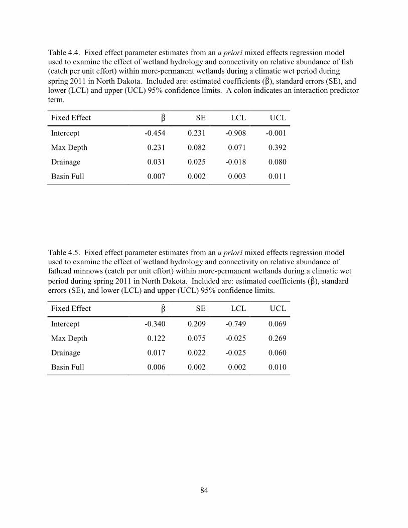
84

Table 4.4. Fixed effect parameter estimates from an a priori mixed effects regression model used to examine the effect of wetland hydrology and connectivity on relative abundance of fish (catch per unit effort) within more-permanent wetlands during a climatic wet period during spring 2011 in North Dakota. Included are: estimated coefficients (β�), standard errors (SE), and lower (LCL) and upper (UCL) 95% confidence limits. A colon indicates an interaction predictor term.


Intercept -0.454 0.231 -0.908 -0.001

Max Depth 0.231 0.082 0.071 0.392

Drainage 0.031 0.025 -0.018 0.080

Basin Full 0.007 0.002 0.003 0.011

Table 4.5. Fixed effect parameter estimates from an a priori mixed effects regression model used to examine the effect of wetland hydrology and connectivity on relative abundance of fathead minnows (catch per unit effort) within more-permanent wetlands during a climatic wet period during spring 2011 in North Dakota. Included are: estimated coefficients (β�), standard errors (SE), and lower (LCL) and upper (UCL) 95% confidence limits.


Intercept -0.340 0.209 -0.749 0.069

Max Depth 0.122 0.075 -0.025 0.269

Drainage 0.017 0.022 -0.025 0.060

Basin Full 0.006 0.002 0.002 0.010

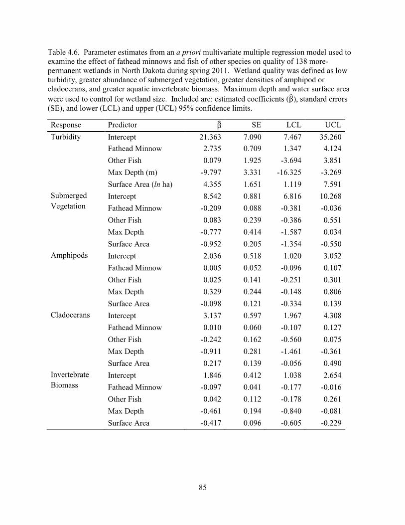
85

Table 4.6. Parameter estimates from an a priori multivariate multiple regression model used to examine the effect of fathead minnows and fish of other species on quality of 138 more-permanent wetlands in North Dakota during spring 2011. Wetland quality was defined as low turbidity, greater abundance of submerged vegetation, greater densities of amphipod or cladocerans, and greater aquatic invertebrate biomass. Maximum depth and water surface area were used to control for wetland size. Included are: estimated coefficients (β�), standard errors (SE), and lower (LCL) and upper (UCL) 95% confidence limits.

Response Predictor β� SE LCL UCL

Turbidity Intercept 21.363 7.090 7.467 35.260 Fathead Minnow 2.735 0.709 1.347 4.124

Other Fish 0.079 1.925 -3.694 3.851

Max Depth (m) -9.797 3.331 -16.325 -3.269

Surface Area (ln ha) 4.355 1.651 1.119 7.591

Submerged Vegetation

Intercept 8.542 0.881 6.816 10.268

Fathead Minnow -0.209 0.088 -0.381 -0.036

Other Fish 0.083 0.239 -0.386 0.551

Max Depth -0.777 0.414 -1.587 0.034

Surface Area -0.952 0.205 -1.354 -0.550

Amphipods Intercept 2.036 0.518 1.020 3.052

Fathead Minnow 0.005 0.052 -0.096 0.107

Other Fish 0.025 0.141 -0.251 0.301

Max Depth 0.329 0.244 -0.148 0.806

Surface Area -0.098 0.121 -0.334 0.139

Cladocerans Intercept 3.137 0.597 1.967 4.308

Fathead Minnow 0.010 0.060 -0.107 0.127

Other Fish -0.242 0.162 -0.560 0.075

Max Depth -0.911 0.281 -1.461 -0.361

Surface Area 0.217 0.139 -0.056 0.490

Invertebrate Biomass

Intercept 1.846 0.412 1.038 2.654

Fathead Minnow -0.097 0.041 -0.177 -0.016

Other Fish 0.042 0.112 -0.178 0.261

Max Depth -0.461 0.194 -0.840 -0.081

Surface Area -0.417 0.096 -0.605 -0.229

86

Discussion

My results provide support for the hypothesis that consolidation drainage has caused an

increase in dispersal of fish and creation of more deep-water refugia where fish are in higher

abundance and can serve as source populations for further dispersal during period of wet climate

conditions (Zimmer et al. 2001a; Anteau 2012). Thus, increased presence and abundance of fish

can be associated to consolidation drainage by the evidence that suggests progressive increases

in water level, less water-level fluctuation in response to climate variability, and ultimately more

connectivity amongst wetlands to larger watersheds as a result of drainage within the catchments

of wetlands (McCauley et al. In Review; Chapter 2). These results are consistent with those of

others that have explained presence of fish as a function of wetland depth and connectedness,

and climate variability (Tonn and Magnuson 1982; Rahel 1984; Magnuson et al. 1998; Hanson et

al. 2005; Herwig et al. 2010). Moreover, the impact of consolidation drainage on wetland

hydrology combined with evidence herein of sustained fish populations suggests that fish

populations are likely to be more-permanent in more wetlands within modified landscapes.

The overall increase in wetland depth that I observed provided more deep-water habitat

that was more suitable for fish to survive and allowed fish to colonize into more wetlands

through connections created by higher water-levels. I observed fish in more wetlands and in

higher abundances than had been observed in the past (Peterka 1989; Anteau and Afton 2008;

Anteau et al. 2011). Further, these increases were correlated with wetlands that filled more of

their topographic basin. While in the short term, some of the observed increases in fish could be

due to prolonged wet climate conditions; over the long-term it appears that consolidation

drainage has potential to permanently increased fish occurrence and abundance. If the climate

were to shift towards more severe dry periods perhaps these trends may be reversed; however, it

87

is unclear what level of drought is required to reverse the trends in increasing water level due to

consolidation drainage (McCauley et al. In Review; Chapter 2). Long-term fish community

trends that include a more-severe dry period as part of a longer period climate cycle will help to

evaluate the permanence of the effects from consolidation drainage.

Numerous studies have linked presence of fish in wetlands to increased turbidity, reduced

submerged vegetation, and reduced abundance of invertebrates (e.g., Scheffer et al. 1993;

Hanson and Butler 1994; Zimmer et al. 2001a; Anteau et al. 2011; Maurer et al. 2014). It is

perhaps safe to assume that fish have a direct negative affect on invertebrate abundance when

they forage upon them (e.g., Hanson and Riggs 1995). However, I did not observe a direct

decrease in amphipod or cladoceran abundance linked to abundance of fish, perhaps because

during an expansion of fish wetlands with good invertebrate abundance also result in great

abundances of fish. My observations were consistent with an indirect mechanisms where greater

fathead minnow abundance results in an increase in turbidity and a decrease in submerged

vegetation which in turn results in a decrease in overall invertebrate biomass including

amphipods, because there was evidence that amphipod abundance was positively related to

submerged vegetation and negatively related to turbidity (Anteau et al. 2011; Chapter 5). Maurer

et al. (2014) also found support for this indirect relationship within wetlands in Iowa. While

evidence from studies that provide snapshots of many wetlands suggests fish have an indirect

impact on aquatic invertebrate communities through increased turbidity and decreased

abundance of submerged vegetation and overall invertebrate biomass, long-term studies of fewer

wetlands or lakes have provided an opportunity to observe stages of changes in trophic structure

as a result of fish introduction and eliminations (Carpenter et al. 1985; Hanson and Butler 1994).

Nonetheless, increased permanence and greater abundance of fish, specifically fathead minnows,

88

in prairie pothole wetlands can be associated with negatively impacting the quality of a wetland

to support waterbird populations that rely on macroinvertebrate prey.

My results also indicated that small wetlands and shallow wetlands had greater

invertebrate biomass than large wetland and deep wetlands. Increased water level and

hydroperiod resulting from consolidation drainage are likely to continue to effect wetland

communities across the region, unless management actions are taken to restore complexes of

wetlands having various hydroperiods and more surface isolation. Increased fish abundance and

turbidity, which are linked to consolidation drainage, can serve as a negative indicator of wetland

quality to support waterbirds. Accordingly, evaluation of distributions of fish and turbidity

within wetlands across landscapes could provide a regional-scale assessment of wetland quality.

If the availability of quality wetlands that can support waterbirds continues to decrease, the

effects are likely to become more noticeable in waterbird populations that rely on invertebrates

within these wetlands to obtain nutrients required for migration and breeding (Afton and

Anderson 2001; Anteau and Afton 2004).

Literature Cited

Afton, A. D., and M. G. Anderson. 2001. Declining scaup populations: a retrospective analysis

of long-term population and harvest survey data. Journal of Wildlife Management

65:781–796.



Anteau, M. J., and A. D. Afton. 2004. Nutrient reserves of lesser scaup (Aythya affinis) during

spring migration in the Mississippi flyway: a test of the spring condition hypothesis. Auk

121:917–929.

89



Anteau, M. J., and A. D. Afton. 2009. Wetland use and feeding by lesser scaup during spring







Carpenter, S. R., J. F. Kitchell, and J. R. Hodgson. 1985. Cascading trophic interactions and lake

productivity. Bioscience 35:634–639.




Cox, R. R., Jr., M. A. Hanson, C. C. Roy, N. H. Euliss, Jr., D. H. Johnson, and M. G. Butler.

1998. Mallard duckling growth and survival in relation to aquatic invertebrates. Journal

of Wildlife Management 62:124–133.

Duffy, W. G. 1998. Population dynamics, production, and prey consumption of fathead minnows

(Pimephales promelas) in prairie wetlands; a bioenergetics approach. Canadian Journal

of Fish and Aquatic Science 54:15–27.

Euliss, N. H., Jr., and D. M. Mushet. 1996. Water-level fluctuation in wetlands as a function of

landscape condition in the Prairie Pothole Region. Wetlands 16:587–593.

90





514.

Gale, W. F., and G. L. Buynak. 1982. Fecundity and spawning frequency of the fathead

minnow—a fractional spawner. Transactions of the American Fisheries Society 111:35–

40.

Hanson, M., and M. Riggs. 1995. Potential effects of fish predation on wetland invertebrates: a

comparison of wetlands with and without fathead minnows. Wetlands 15:167–175.

Hanson, M. A., and M. G. Butler. 1994. Responses of plankton, turbidity, and macrophytes to

biomanipulation in a shallow prairie lake. Canadian Journal of Fish and Aquatic Science

51:1180–1188.

Hanson, M. A., K. D. Zimmer, M. G. Butler, B. A. Tangen, B. R. Herwig, and N. H. Euliss, Jr.

2005. Biotic interactions as determinants of ecosystem structure in prairie wetlands: an

example using fish. Wetlands 25:764–775.

Held, J. W., and J. J. Peterka. 1974. Age, Growth, and Food Habits of the Fathead Minnow,

Pimephales promelas, in North Dakota Saline Lakes. Transactions of the American

Fisheries Society 103:743–756.

Herwig, B. R., and K. D. Zimmer. 2007. Population ecology and prey consumption by fathead

minnows in prairie wetlands: importance of detritus and larval fish. Ecology of

Freshwater Fish 16:282–294.

91

Herwig, B. R., K. D. Zimmer, M. A. Hanson, M. L. Konsti, J. A. Younk, R. W. Wright, S. R.

Vaughn, and M. D. Haustein. 2010. Factors influencing fish distributions in shallow lakes

in prairie and prairie-parkland regions of Minnesota, USA. Wetlands 30:609–619.








Leibowitz, S. G., and K. C. Vining. 2003. Temporal connectivity in a prairie pothole complex.


Magnuson, J. J., W. M. Tonn, A. Banerjee, J. Toivonen, O. Sanchez, and M. Rask. 1998.

Isolation vs. extinction in the assembly of fishes in small northern lakes. Ecology

79:2941–2956.

Maurer, K. M., T. W. Stewart, and F. O. Lorenz. 2014. Direct and indirect effects of fish on

invertebrates and tiger salamanders in prairie pothole wetlands. Wetlands 34:735–745.





Wetlands 34:1123–1132.

92

Merkey, D. H. 2006. Characterization of wetland hydrodynamics using HGM and

subclassification methods in southeastern Michigan, USA. Wetlands 26:358–367.

Nyman, J. A., and R. H. Chabreck. 1996. Some effects of 30 years of weir-management on

coastal march aquatic vegetation and implications for waterfowl management. Gulf of

Mexico Science 14:16–25.





Rahel, F. J. 1984. Factors structuring fish assemblages along a bog lake successional gradient.

Ecology 65:1276–1289.



Swanson, G. A., and H. K. Nelson. 1970. Potential influence of fish rearing programs on

waterfowl breeding habitat. In E. Schneberger (ed) Symposium on the management of

midwestern winterkill lakes. North Central Division of the American Fisheries Socitey,

Winnipeg, Manitoba, Canada, pp 65–71.

Tonn, W. M., and J. J. Magnuson. 1982. Patterns in the species composition and richness of fish

assemblages in northern Wisconsin lakes. Ecology 63:1149-1166.



93

Zimmer, K. D., M. A. Hanson, and M. G. Butler. 2000. Factors influencing invertebrate

communities in prairie wetlands: a multivariate approach. Canadian Journal of Fisheries

and Aquatic Sciences 57:76–85.

Zimmer, K. D., M. A. Hanson, and M. G. Butler. 2001a. Effects of fathead minnow colonization

and removal on a prairie wetland ecosystem. Ecosystems 4:346–357.

Zimmer, K. D., M. A. Hanson, M. G. Butler, and W. G. Duffy. 2001b. Size distribution of

aquatic invertebrates in two prairie wetlands, with and without fish, with implications for

community production. Freshwater Biology 46:1373–1386.

94

CHAPTER 5. AMPHIPOD DENSITIES REMAIN LOW FOLLOWING WATER-

LEVEL FLUCTUATION IN PRAIRIE POTHOLE WETLANDS

Abstract

Variability in amphipod abundance and productivity within wetlands of the Prairie

Pothole Region is thought to have been historically driven by inter-annual fluctuations of water

levels that facilitated nutrient cycling. However, landscape modifications have altered wetland

hydrologic regimes and responses to climate variability, namely water-level fluctuation.

Consequent changes in amphipod abundance and productivity may impact waterbird

populations, because amphipods are important forage for migrating and breeding waterbirds in

the region. In 2004–2005, amphipods densities were low across the Prairie Pothole Region

following a period of high and stable water levels, perhaps due to lack of water-level fluctuation.

I tested whether subsequent water-level fluctuations in the prairie pothole wetlands in North

Dakota influenced a change in density of Gammarus lacustris and Hyalella azteca (hereafter

Gammarus and Hyalella, respectively) from prior to a dry period in 2006–2008 to after wetlands

re-flooded in 2010–2011. Wetland water surface area decreased 22% (±2.0S E) during the dry

period, and then wetlands re-flooded to 7% (±1.1 SE) greater than initial area during the wet

period. However, Gammarus and Hyalella densities remained generally low in North Dakota;

specifically, Gammarus densities did not change and Hyalella decreased slightly. Further,

density of both species decreased where extensive historical wetland drainage occurred within

catchments of surveyed wetlands; however, both species increased where wetlands filled more of

their topographic basins. My findings suggest that previously reported low region-wide densities

of amphipods were not a result of a sustained wet period; rather they may be the result of

landscape modifications that alter wetland hydrology.

95

Introduction

Amphipods are a common crustacean in semipermanent and permanent wetlands of the

Prairie Pothole Region, and Gammarus lacustris and Hyalella azteca (hereafter Gammarus and

Hyalella, respectively) are the two most abundant species within wetlands of the region (Kantrud

et al. 1989; Anteau and Afton 2008). The density of amphipods can serve as an indicator of

wetland and water quality because amphipods are sensitive to disturbances in uplands, invasive

species, and contaminants (Grue et al. 1988; Tome et al. 1995; Duan et al. 2000; Anteau and

Afton 2008; Hentges and Stewart 2010; Anteau et al. 2011). Rich in lipids and proteins,

amphipods are an important forage for locally breeding waterbirds and for those bound for other

breeding areas that must acquire and maintain nutrient reserves while migrating through the

region (Batt et al. 1989; Swanson and Duebbert 1989; Anteau and Afton 2006, 2011).

Amphipod densities in the spring are an indicator of forage availability for spring migrating and

breeding waterbirds and indicate previous-year productivity and overwinter survival of

amphipods (Lindeman and Clark 1999; Anteau and Afton 2009a). Therefore, the quality of a

wetland to support waterbirds can be assessed in the spring using the density of adult amphipods

that survived over winter (Anteau and Afton 2008).

Historically, water levels in wetlands fluctuated in response to climate fluctuations

between wet and dry periods (Kantrud et al. 1989; Euliss et al. 1999; Euliss et al. 2004; Anteau

2012; McCauley et al. In Review). It is thought that hydrologic responses of wetlands to these

wet–dry periods are one of the primary drivers of productivity and density of aquatic

invertebrates in the prairie pothole wetlands (Euliss et al. 1999). High and stable water levels

inhibit nutrient cycling, but the drying of wetlands or portions of wetlands allows for nutrient

cycling and a subsequent pulse of productivity after wet conditions return (Euliss et al. 1999).

96

Similarly, wetlands likely receive increases in nutrients when uplands are inundated by extreme

or consecutive wet years. Accordingly, temporal position within wet–dry periods likely affects

abundance of aquatic invertebrates and ultimately populations of waterbirds that are dependent

on the nutritional resources provided by prairie pothole wetlands. However, landscape

modifications can alter water-level responses to climate variability (Post van der Burg et al. In

Prep.; McCauley et al. In Review; Chapter 2), potentially disrupting linkages among wet–dry

periods, wetland productivity, and waterbird populations (Batt et al. 1989).

Abundance and quality of wetlands in North Dakota has declined due to landscape

modifications, primarily agriculture (Dahl 1990; Anteau and Afton 2008; Bartzen et al. 2010). A

common agricultural practice aimed at increasing tillable acreage is to consolidate water from

smaller, less-permanent wetlands into larger, more-permanent wetlands (Krapu et al. 2004;

Anteau 2012). This practice alters hydrology of wetlands that receive consolidated water by

increasing their size and changing the way wetlands respond to climate fluctuations (Anteau

2012; Post van der Burg et al. In Prep.; McCauley et al. In Review; Chapter 2). Wetlands with

water levels that are near the topographic basin spill point have attenuated water-level fluctuation

which can impact pulses of productivity once experienced in these wetlands.

Existing drainage networks and high water levels increase surface water connections

among remaining wetlands that can serve as corridors for fish to distribute into new wetlands and

find overwinter refugia. A high abundance of fish can both directly (through predation) and

indirectly (e.g., through increased turbidity or reduction of submerged aquatic vegetation) impact

density of invertebrates in wetlands (Hanson and Butler 1994; Zimmer et al. 2000; Hanson et al.

2005; Anteau and Afton 2008; Anteau et al. 2011). Tiger salamanders (Ambystoma tigrinum) in

high abundance can also decrease densities of amphipods through predation (Olenick and Glee

97

1981; Kantrud et al. 1989; Macneil et al. 1999; Benoy 2005); although, native populations of

tiger salamander also have been negatively impacted by upland modification (Balas et al. 2012;

Mushet et al. 2014).

Conversion of uplands surrounding wetlands from grasslands to cropland may indirectly

decrease quality of wetlands by increasing sediment delivered by runoff water and wind thereby

increasing turbidity of the water (Gleason and Euliss 1998). Turbidity and high sediment loads

reduce the abundance of submerged aquatic vegetation and invertebrates in wetlands (Gleason

and Euliss 1998; Anteau and Afton 2008; Anteau et al. 2011). However, buffers of grassland

between wetlands and tilled land can reduce the effect of sedimentation and negative impacts on

invertebrate abundance (Castelle et al. 1994; Anteau et al. 2011).

In 2004–2005, amphipod densities were low across the Prairie Pothole Region compared

to historical records (Anteau and Afton 2008), perhaps due to landscape modifications (Anteau

and Afton 2008; Anteau et al. 2011). However, most of the region in the years prior to 2004 and

2005 experienced a regime of relatively high and stable water levels since 1993; therefore,

amphipod numbers could have been low due to a period of little inter-annual water-level

variation during which nutrients limited productivity (Euliss et al. 1999; Euliss et al. 2004).

Many parts of the Prairie Pothole Region in North Dakota experienced moderate to severe

drought during 2006–2008 (NCDC 2014), making it possible for basins to have lower water

levels and subsequent nutrient cycling (Euliss et al. 1999). In spring 2009, wet conditions

returned for most prairie wetlands in North Dakota. Thus, if amphipod densities were low in

2004–2005 due to the temporal position within wet–dry climate fluctuations, then I expected

amphipod densities would increase after water levels increased in 2009. However, if landscape

98

modifications disturbed water-level fluctuations or have had other influences upon amphipods, I

expected densities to remain low.

In this chapter, I tested if water-level dynamics effected the change in density of

amphipods from prior to the dry period in 2006–2008 to after wetlands re-flooded. I also

evaluated the influence of landscape modifications, the presence of fish and salamanders on the

change in amphipod density.

Methods

Study Area

I returned to wetlands within the Prairie Pothole Region of North Dakota (Figure 5.1) that

were previously randomly selected and surveyed once in 2004 or 2005 (hereafter, 2004/05) by

Anteau and Afton (2008; n = 153). These were lacustrine semipermanent and shallow-water

permanent wetlands (Cowardin et al. 1979) that must have had an open-water area larger than

120 m across to be surveyed in 2004/05. In 2004/05, if reselection in the field was necessary, the

nearest suitable semipermanent wetland was surveyed. In each year 2010 and 2011, I returned to

126 of the original 153 wetlands. I did not survey the remaining wetlands because I could not

gain permission to access private lands, or wetlands had been amalgamated with larger water

bodies (e.g., Devils Lake). Based on National Wetland Inventory classification (NWI; U.S. Fish

and Wildlife Service 2003), 67% of our wetlands were semipermanent, 3% seasonal, and the rest

being permanent wetlands or shallow-water lakes. Those wetlands classified by NWI as

seasonal were wetlands reselected in the field in 2004/05 that were more characteristic of

semipermanent wetlands at time of field assessment.

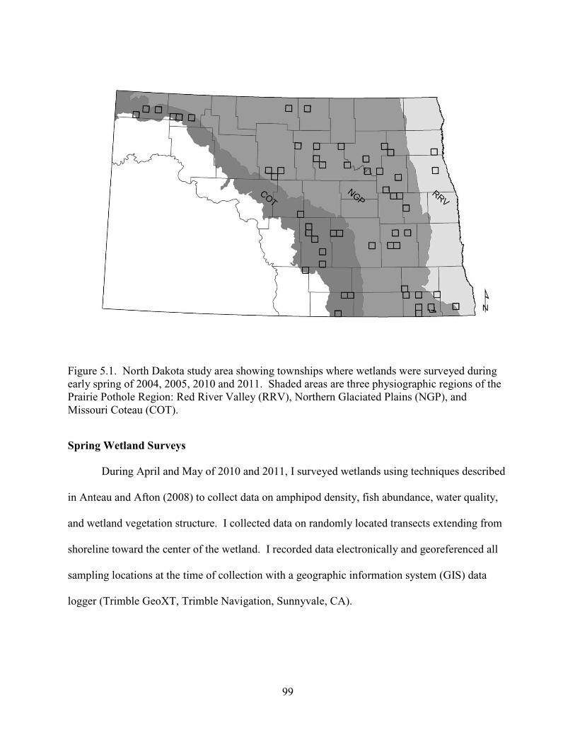
99

Figure 5.1. North Dakota study area showing townships where wetlands were surveyed during early spring of 2004, 2005, 2010 and 2011. Shaded areas are three physiographic regions of the Prairie Pothole Region: Red River Valley (RRV), Northern Glaciated Plains (NGP), and Missouri Coteau (COT).

Spring Wetland Surveys

During April and May of 2010 and 2011, I surveyed wetlands using techniques described

in Anteau and Afton (2008) to collect data on amphipod density, fish abundance, water quality,

and wetland vegetation structure. I collected data on randomly located transects extending from

shoreline toward the center of the wetland. I recorded data electronically and georeferenced all

sampling locations at the time of collection with a geographic information system (GIS) data

logger (Trimble GeoXT, Trimble Navigation, Sunnyvale, CA).

100

Amphipod densities

I sampled amphipods in open water using a D-shaped sweep net (1,200 µm mesh, 0.072

m2 opening, WARD’S Natural Science, Rochester, NY) at four amphipod-sampling transects

(hereafter primary transects). Sampling stations at each transect were located at 10 and 60 m

from the shoreline or emergent vegetation to open-water interface. Sample locations were

adjusted along transects to ensure the station depth was between 0.5 and 3 m (see Anteau and

Afton 2008). I recorded depth at each sampling station to the nearest 0.1 m. At each station, a

sweet-net sample consisted of a sweep across the bottom for a distance equal to the water depth,

and a sweep up through the water column. I calculated the volume of water sampled (VS; m3)

with a sweep net using the following equation (Anteau and Afton 2008):

VS = 2(∑ Di ) x SN,

where Di = depth at each sampling location and SN = area of the sweep-net opening (0.072 m2).

Vegetation or debris that was brought up in the sweep net was included in the sample, unless

>50% of the object was hanging outside the net. I composited the samples into 10- and 60-m

samples for each wetland, and samples were chilled with ice then frozen within 8 hours of

collection. In the laboratory, I allowed the samples to thaw, and then I sorted and counted

amphipods by species.

Wetland habitat

After a sweep-net sample had been taken at a station, I surveyed the abundance of

submerged aquatic vegetation along a perpendicular sub-transect originating at the sampling

station. I recorded vegetation presence/absence of 10 rake grabs (36-tine, 91.4 cm wide Lake

Rake, Ben Meadows Co., Janesville, WI) spaced approximately 1 m apart on each sub-transect

(Nyman and Chabreck 1996; Anteau and Afton 2008). One rake grab consisted of the rake being

101

gently placed on the wetland bottom and then pulled straight up to the surface. The rake was

cleaned of vegetation after each grab.

At four regularly spaced locations that approximated quarters of each wetland I measured

turbidity (± 2 nephelometric turbidity units [NTU]), electrical conductivity (± 1µS), and water

temperature (± 1ºC). These measurements were taken prior to any disturbance by other sampling

methods.

Fish and salamander communities

I used minnow traps and an experimental gill net in wetlands to determine relative

abundance of fish and salamanders (see Anteau and Afton 2008). I set five Gee-style minnow

traps with 6.35-mm mesh at the emergent vegetation to open-water interface (or equivalent

position from the shoreline if no emergent vegetation is present) at five transects. I set the

monofilament experimental gill net (21 × 2 m with seven 3-m panels ranging in mesh size from

1.9–7.6 cm) at a transect perpendicular to the shoreline with the small mesh end of the net at the

emergent vegetation to open-water interface (or equivalent position from the shoreline if no

emergent vegetation was present). Minnow traps and the gill net were deployed for 12–24 hours

including an overnight period. At the time of trap and gill net retrieval, I sorted and counted fish

by species and by length category (<5, 5–10, 10–20, 20–40, >40 cm) and measured body length

of each salamander (±1 cm).

I classified all captures into one of four categories: fathead minnows (Pimephales

promelas), other small fish species typically <10 cm (e.g., other minnows [Cyprinidae], darters

[Anhingidae], and sticklebacks [Gasterosteidae]), large fish species typically >10 cm (e.g.

northern pike [Esox lucius], walleye [Sander vitreus], yellow perch [Perca flavescens], sunfishes

[Lepomis spp.], and bullhead and catfish [Ictaluridae]), and salamanders. I calculated catch per

102

unit effort (relative abundance) for each gear type by dividing the number of captures of each

class by the hours the gear was in the water. For each class, I summed the quotients of the two

gear types.

In 2011 I used the complete array of traps and a gill net in all wetlands surveyed.

However, in 2010, I only used the five 6.35-mm mesh minnow traps in 75% of wetlands

surveyed, and I did not adequately sample fish in the remaining 25% of wetlands. Therefore, I

relied on the complete data collected in 2011 for my analyses.

Water depth

To estimate change in depth among surveys of 2004/05 (Anteau and Afton 2008) and

surveys of 2010 and 2011, I measured water depth (± 0.1 m) at 10 locations estimated to be 10 m

into open water from either the shoreline or emergent vegetation to open-water interface for

2004/05. When waves were present, I recorded the average depth between wave crests and

troughs. Prior to field work, I delineated the shoreline or emergent vegetation to open-water

interface of each wetland using imagery (National Agricultural Imagery Program, U.S.

Department of Agriculture; hereafter NAIP) acquired in the summer (July) prior to each spring

survey by Anteau and Afton (2008). I used the imagery from the previous year because it better

represents the location of the emergent vegetation to open-water interface that Anteau and Afton

(2008) used to locate their sampling locations. I digitized the interface by using GIS software at

a scale of 1:5,000. I offset (i.e. buffered) the digitized open-water interface by 10 m in the

direction of the wetland center to approximate locations of 2004/05 sampling. I derived my 10

random points from the 10-m buffer, but I constrained point locations so there is a minimum

distance of 40 m between points. I loaded the random points onto the Trimble GeoXT to

navigate to sampling locations. Sample locations found within the emergent vegetation ring

103

were recorded as such, because different dynamics of sedimentation and accumulation of

organics were expected. Additionally, in 2011, I measured depth at four georeferenced locations

where 10-m depth sampling occurred in 2010.

Water surface area

I used water surface area delineated for each surveyed wetland by photointerpretation of

National Agriculture Imagery Program (NAIP; U.S. Department of Agriculture) aerial imagery

for 2003–2006 and 2009–2010 (McCauley et al. In Review). Photointerpretation was performed

while images were viewed as panchromatic instead of true-color, because they were done as part

of a larger study that involved panchromatic imagery (see McCauley et al. In Review). Where

the waterline was obscured by emergent vegetation, the waterline was approximated to be

halfway between the emergent-vegetation to open-water interface and clearly identifiable upland.

NAIP imagery was not available for 2007 and 2008. For those years I used wetland water

surface area delineated once in either 2007 or 2008 using high-resolution digital elevation model

(DEM; source data: 1 m pixel lidar; Data available from the U.S. Geological Survey) or ~1.25 m

pixel interferometric synthetic aperture radar (IfSAR) orthorectified image (Intermap

Technologies, Inc., Englewood, Colorado).

Catchments


by McCauley et al. (In Review) that were delineated using high-resolution digital elevation

models to detect the portion of the landscape where surface water flows into the focal wetland.

These catchments included more-intermittent wetlands and their catchments (McCauley and

Anteau 2014). DEM source data included 1 m pixel lidar (data available from the U.S.

Geological Survey) or ~1.25 m pixel interferometric synthetic aperture radar (IfSAR; Intermap

104

Technologies, Inc., Englewood, Colorado). I used catchment size in my analysis, but I also used

the extent of the catchment to define the area to assess land use effects upon wetlands (McCauley

and Anteau 2014). For logistical reasons associated with assembling landscape variables, such

as amount of wetland area drained, I used catchments truncated to a 2.5 km maximum radius

from the wetland basin for 46% of catchments because they were large or highly irregular in

shape. The 2.5-km radius encompassed >90% of the total catchment area for 68% of

catchments. Landscape conditions within these 2.5-km truncated catchments should represent

the condition of the full catchment, and the conditions nearest the wetland basin likely influence

the basin most. Therefore, I assume the 2.5-km-truncated catchment provided a reasonable area

to evaluate impacts of land use in this system and are an improvement over the simply buffering

around a wetland a set distance, a common practice (McCauley and Anteau 2014).

Catchment drainage

I used estimates of the percent of the catchment area that was drained wetland during

2003–2010 estimated from multiple data sources, including: aerial photographs, DEM, NWI, and

spatially explicit soil data (see McCauley et al. In Review). Wetlands were identified as drained

if they were present in historical photographs (dating back to 1937) but not present in current

photographs, or if the wetlands were identified as part of a drainage network. Significant

drainage occurred prior to 2003 in my study area; however, I found negligible evidence of

additional drainage after 2003.

Basin area

Within a catchment, I defined the basin as the topographic depression that collects

surface water and which is isolated from basins of other wetlands of an equal or more permanent

hydroperiod. I calculated the maximum potential water surface area of each basin using the

105

high-resolution DEMs (3 m pixel lidar or 5 m pixel IfSAR) to find the elevation at which water

flows out of the basin (i.e., spill point) and then delineated the area at that spill point elevation

within the basin. Because I predicted that wetlands in basins that were near full or that were full

would have less surface area dynamics, I calculated the proportion of the basin that the focal

wetland filled at the start of each climate phase. I used a logit transformation of the proportion-

basin-full variable × 0.1 for use in my analysis.


I separately tested if Gammarus and Hyalella densities were different among years (i.e.,

position in climatic wet–dry fluctuations) and among regions using a two-way analysis of

variance (ANOVA), including an interaction of the two factors. I included region in this a priori

test because Anteau and Afton (2008) found differences in density by physiographic region, and

it is possible that amphipod productivity varied by region during the period of study. Because

amphipod densities followed a skewed-right distribution, I natural logarithm (+1)-transformed

densities to meet assumptions of normality (Devore 2000). I calculated geometric least-squares

mean density of both species for each year by region using estimates from the two-way ANOVA

interaction. I plotted back-transformed geometric least-squares means and 95% confidence

intervals. I evaluated main effects from back-transformed estimated means and 95% confidence

intervals of two-way ANOVAs for each species that did not include the interaction. Means

were interpreted as different if the confidence interval did not overall the mean of the other level.

For each Gammarus and Hyalella, I calculated the change in density for year one as the

difference between the 2004/05 and 2010 samples, and for year two as the difference between

the 2004/05 and 2011 samples. If a species was not found in any of the three sampling attempts,

the wetland was removed from change in density analyses for that species. For both species, the

106

distribution of change in density had long tails, so I natural logarithm (+1) -transformed the

absolute values of the difference and then resigned the transformed value. I analyzed data from

two years of follow-up sampling (i.e., 2010 and 2011) to account for any lag in the productivity-

response to fluctuating water levels; however, I expected amphipod colonization and production

to be high during 2009 which was the first year of the wet period.

Prior to creating a general model for change in amphipod density, I evaluated changes in

response to landscape modification and water-level fluctuation in year one and year two.

Specifically, I calculated geometric least-squares mean changes in density separately for both

species of amphipods in wetlands classified into categories delimited by one-third quantiles for

1) percent catchment area that was drained wetland; 2) percent wetland area that was re-flooded

after drawdown during the drying period; and 3) percent wetland area that was newly flooded

beyond 2003–2005 water levels. I interpreted an effect as present if the 95% confidence interval

did not overlap zero. I plotted back-transformed geometric least-squares means and 95%

confidence intervals.

To uncouple potential effects of landscape modifications from those of water-level

fluctuations, I tested the effect of water-level fluctuation on changes in amphipod density for

each species within a general mixed-effects regression analysis (Package lme4 in R Statistical

Computing Environment; R Development Core Team 2010; Bates et al. 2011). I evaluated

water-level fluctuation effects in an a priori model by using natural logarithm (+1)-transformed

area of wetland that was re-flooded after drawdown during the drying period and natural

logarithm (+1)-transformed area of wetland that was newly flooded beyond 2003–2005 water

levels. I included additional fixed effect variables to control for maximum depth observed in

2004/05, wetland connectedness by means of percent basin full and percent catchment area that

107

was drained wetland. I found only weak evidence of collinearity among fixed effects (all |r| <

0.32). I included a repeated measures term for wetland by year and a random effect term for

sampled township in the models to accommodate my sampling design.

I conducted a second analysis on change in amphipod density that included only wetlands

for which a complete set of fish abundance, salamander abundance, water-quality parameters and

wetland vegetation variables were available in 2004/05 and 2011 samples. I created five variable

suites representing alternative hypotheses as to influences on change in amphipod density,

including: 1) water-level dynamics with re-flood area, newly flooded area, and basin full; 2)

water quality with electrical conductivity, turbidity, and submerged aquatic vegetation

abundance; 3) fish change in occurrence and/or change in density for any species; 4) fathead

minnow change in occurrence and/or change in density; and, 5) salamander change in occurrence

and/or change in density. Prior to creating multiple models I evaluated change in occurrence and

change in density of fish, fathead minnows, and salamanders each separately in a full model that

included all of the other suites. Change in occurrence resulted in the better model for each fish,

fathead minnows, and salamander; therefore change in occurrence was used in all subsequent

models. I created multiple models from all combination of variable suites, with the exception of

change in occurrence of fish of any species and change in occurrence of fathead minnows being

in the same model, and I included an intercept only model. I found only weak evidence of

collinearity among fixed effect variables that were included in the same model (all |r| < 0.40). I

used an information theoretical approach to select and interpret the single most parsimonious

model using Akaike’s Information Criterion adjusted for small sample size (AICC; Burnham and

Anderson 2002).

108

I determined fixed effect variables to be important if 95% confidence intervals did not

include zero. I reported goodness-of-fit for mixed effects models using marginal and conditional

R2 (Nakagawa and Schielzeth 2013).

Results

During 2010 and 2011, I resurveyed 126 wetlands that were initially surveyed in 2004/05

(Anteau and Afton 2008). At the time of initial sampling in 2004/05, wetlands averaged 63 ha of

water surface area (range = 1–849 ha, median = 24 ha) and 1.3 m maximum water depth (range =

0.5–3.0 m, median = 1.0 m). During the dry period in 2006–2008, wetland water surface area

had decreased 22% (±2.0 SE). During the following wet period in 2009–2011, average wetland

water surface area was 16% (±1.7 SE) greater than the previously exposed area that had been re-

flooded and 7% (±1.1 SE) greater than the initial area. On average, focal wetland basins were

61% (range = 1% to >100%, quartiles = 43%, 61%, 83%) and 65% (range = 1% to >100%,

quartiles = 48%, 68%, 87%) full during 2010 and 2011, respectively. During 2011, focal

wetland basins were 3% more full than during 2004/05 (range = -43% to 46%, quartiles = -4%,

2%, and 8%).

Gammarus were present in 34%, 25%, and 31% of wetlands in 2004/05, 2010, and 2011,

respectively. The region-by-year interaction was not important for explaining Gammarus

densities (F4, 369 = 0.19, P = 0.94; Figure 5.2). Gammarus densities were different among

regions (F2, 373 = 6.06, P < 0.01), as densities were greater in NGP than in COT and RRV (Table

5.1). However, Gammarus densities did not differ among years (F2, 373 = 0.85, P = 0.43; Table

5.2).

109

Figure 5.2. Back-transformed geometric least squares mean densities (m-3) and 95% lower (LCL) and upper (UCL) confidence limits of Gammarus lacustris observed in 2004 or 2005 (circle), 2010 (square), and 2011 (triangle) in three physiographic regions of the Prairie Pothole Region of North Dakota: Red River Valley (RRV), Northern Glaciated Plains (NGP), and Missouri Coteau (COT).

Gam

mar

us

(m-3

)

COT NGP RRV

02

46

810

2004/0520102011

110

Table 5.1. Back-transformed geometric least squares mean densities (m-3) and 95% lower (LCL) and upper (UCL) confidence limits of Gammarus lacustris and Hyalella azteca observed during 2004 or 2005, 2010, and 2011 in N number of wetlands within three physiographic regions of the Prairie Pothole Region of North Dakota.

Region N Mean LCL UCL

Gammarus lacustris

Missouri Coteau 44 0.49 0.20 0.86

Northern Glaciated Plains 74 1.28 0.93 1.70

Red River Valley 8 0.20 -0.28 1.01

Hyalella azteca

Missouri Coteau 44 6.90 4.64 10.06

Northern Glaciated Plains 74 7.32 5.42 9.79

Red River Valley 8 5.40 1.91 13.09

Table 5.2. Back-transformed geometric least squares mean densities (m-3) and 95% lower (LCL) and upper (UCL) confidence limits of Gammarus lacustris and Hyalella azteca observed in 126 wetlands within the Prairie Pothole Region of North Dakota.

Sampling Year Mean LCL UCL

Gammarus lacustris

2004 or 2005 1.10 0.67 1.63

2010 0.70 0.36 1.13

2011 0.89 0.51 1.37

Hyalella azteca

2004 or 2005 9.76 6.62 14.18

2010 4.91 3.19 7.34

2011 7.17 4.79 10.53

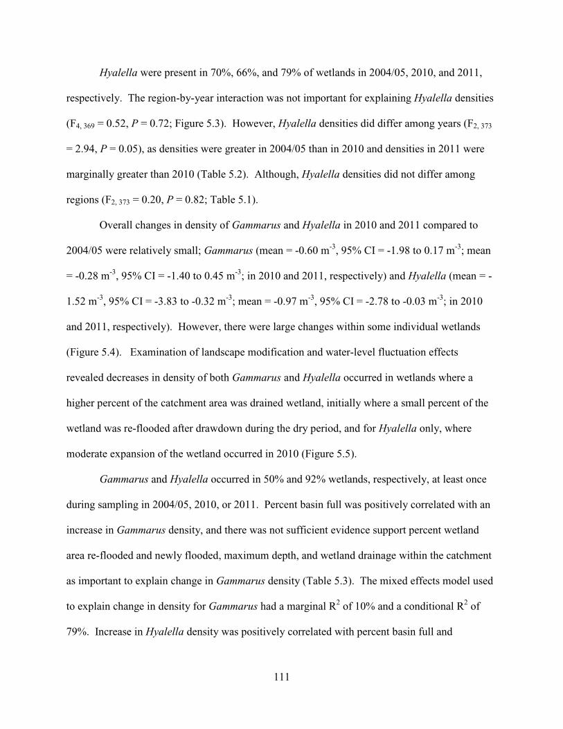
111

Hyalella were present in 70%, 66%, and 79% of wetlands in 2004/05, 2010, and 2011,

respectively. The region-by-year interaction was not important for explaining Hyalella densities

(F4, 369 = 0.52, P = 0.72; Figure 5.3). However, Hyalella densities did differ among years (F2, 373

= 2.94, P = 0.05), as densities were greater in 2004/05 than in 2010 and densities in 2011 were

marginally greater than 2010 (Table 5.2). Although, Hyalella densities did not differ among

regions (F2, 373 = 0.20, P = 0.82; Table 5.1).

Overall changes in density of Gammarus and Hyalella in 2010 and 2011 compared to

2004/05 were relatively small; Gammarus (mean = -0.60 m-3, 95% CI = -1.98 to 0.17 m-3; mean

= -0.28 m-3, 95% CI = -1.40 to 0.45 m-3; in 2010 and 2011, respectively) and Hyalella (mean = -

1.52 m-3, 95% CI = -3.83 to -0.32 m-3; mean = -0.97 m-3, 95% CI = -2.78 to -0.03 m-3; in 2010

and 2011, respectively). However, there were large changes within some individual wetlands

(Figure 5.4). Examination of landscape modification and water-level fluctuation effects

revealed decreases in density of both Gammarus and Hyalella occurred in wetlands where a

higher percent of the catchment area was drained wetland, initially where a small percent of the

wetland was re-flooded after drawdown during the dry period, and for Hyalella only, where

moderate expansion of the wetland occurred in 2010 (Figure 5.5).

Gammarus and Hyalella occurred in 50% and 92% wetlands, respectively, at least once

during sampling in 2004/05, 2010, or 2011. Percent basin full was positively correlated with an

increase in Gammarus density, and there was not sufficient evidence support percent wetland

area re-flooded and newly flooded, maximum depth, and wetland drainage within the catchment

as important to explain change in Gammarus density (Table 5.3). The mixed effects model used

to explain change in density for Gammarus had a marginal R2 of 10% and a conditional R2 of

79%. Increase in Hyalella density was positively correlated with percent basin full and

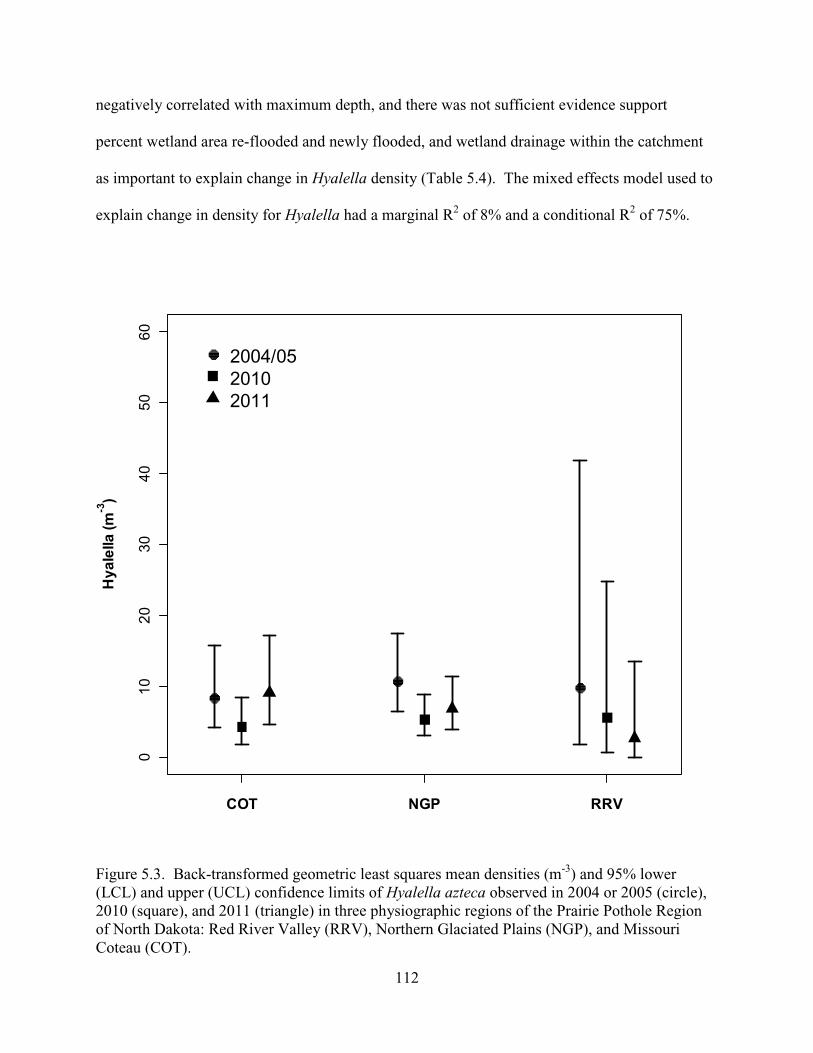
112

negatively correlated with maximum depth, and there was not sufficient evidence support

percent wetland area re-flooded and newly flooded, and wetland drainage within the catchment

as important to explain change in Hyalella density (Table 5.4). The mixed effects model used to

explain change in density for Hyalella had a marginal R2 of 8% and a conditional R2 of 75%.

Figure 5.3. Back-transformed geometric least squares mean densities (m-3) and 95% lower (LCL) and upper (UCL) confidence limits of Hyalella azteca observed in 2004 or 2005 (circle), 2010 (square), and 2011 (triangle) in three physiographic regions of the Prairie Pothole Region of North Dakota: Red River Valley (RRV), Northern Glaciated Plains (NGP), and Missouri Coteau (COT).

Hya

lella

(m-3

)

COT NGP RRV

010

2030

4050

60

2004/0520102011

113

Figure 5.4. Distribution of change in density (m-3) of Gammarus lacustris and Hyalella azteca from 2004 or 2005 to 2010 and 2011 observed in wetlands of the Prairie Pothole Region of North Dakota.

Change in Density (m-3)

Per

cent

of T

otal

0

20

40

60

80

100Gammarus 2004/05 to 2010 Gammarus 2004/05 to 2011

0

20

40

60

80

100

-1500 -1000 -500 0 500 1000

Hyalella 2004/05 to 2010

-1500 -1000 -500 0 500 1000

Hyalella 2004/05 to 2011

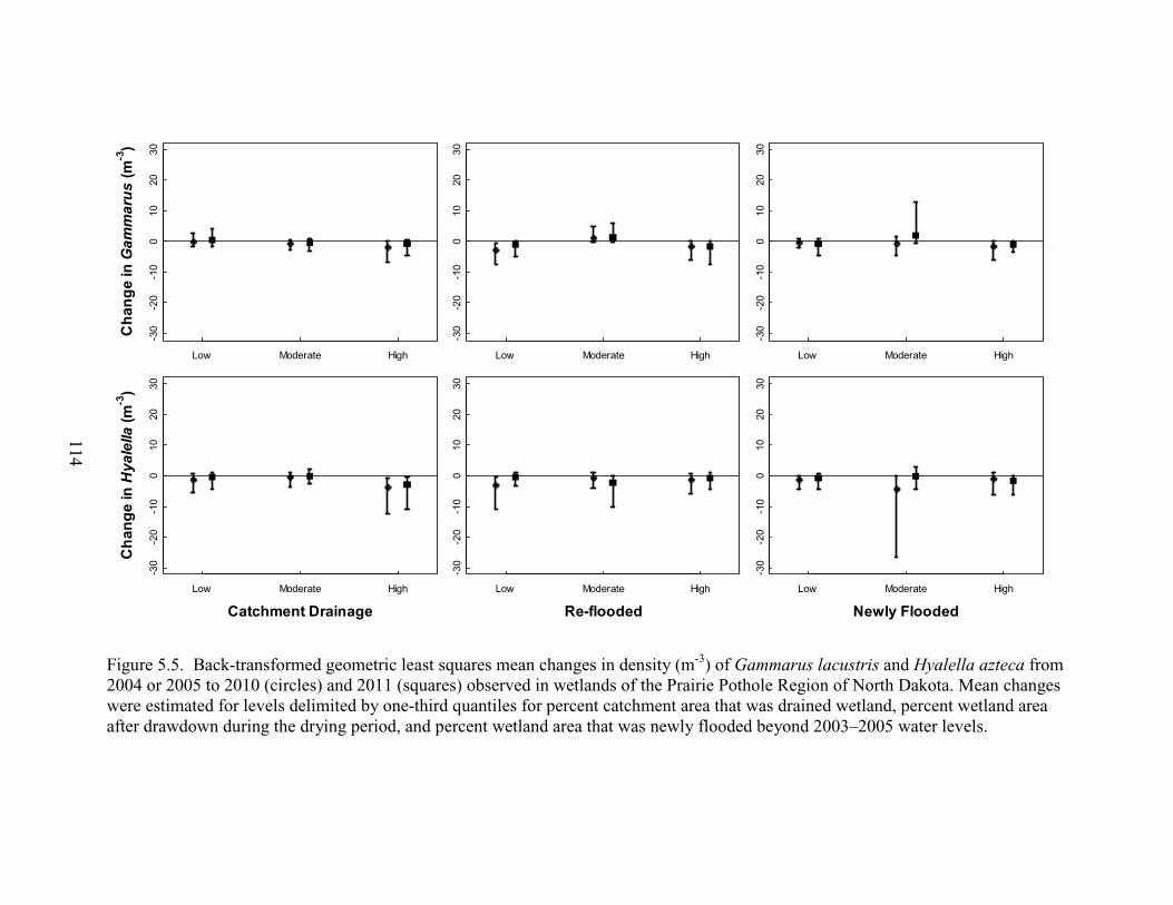
114

Figure 5.5. Back-transformed geometric least squares mean changes in density (m-3) of Gammarus lacustris and Hyalella azteca from 2004 or 2005 to 2010 (circles) and 2011 (squares) observed in wetlands of the Prairie Pothole Region of North Dakota. Mean changes were estimated for levels delimited by one-third quantiles for percent catchment area that was drained wetland, percent wetland area after drawdown during the drying period, and percent wetland area that was newly flooded beyond 2003–2005 water levels.

Low Moderate High

-30

-20

-10

010

2030

Ch

ang

e in

Gam

mar

us

(m-3

)

Low Moderate High

-30

-20

-10

010

2030

Low Moderate High

-30

-20

-10

010

2030

Low Moderate High

-30

-20

-10

010

2030

Ch

ang

e in

Hya

lella

(m-3

)

Catchment Drainage

Low Moderate High

-30

-20

-10

010

2030

Re-flooded

Low Moderate High

-30

-20

-10

010

2030

Newly Flooded

115

Table 5.3. Estimated coefficients (β�) and standard errors for fixed effects within an a priori model used to examine the effect of water-level dynamics on change in density of Gammarus lacustris in wetlands of North Dakota from 2004 or 2005 to 2010 and 2011.


Intercept -1.226 0.957 -3.101 0.650

Re-flooded -0.109 0.258 -0.615 0.397

Newly Flooded -0.215 0.181 -0.569 0.138

Maximum Depth 0.009 0.371 -0.719 0.736

Drainage -0.154 0.134 -0.417 0.109

Basin Full 0.022 0.010 0.002 0.042

Table 5.4. Estimated coefficients (β�) and standard errors for fixed effects within an a priori model used to examine the effect of water-level dynamics on change in density of Hyalella azteca in wetlands of North Dakota from 2004 or 2005 to 2010 and 2011.


Intercept -0.564 0.895 -2.318 1.191

Re-flooded -0.201 0.260 -0.710 0.309

Newly Flooded 0.032 0.230 -0.418 0.483

Maximum Depth -1.058 0.401 -1.844 -0.273

Drainage -0.163 0.106 -0.371 0.046

Basin Full 0.025 0.011 0.005 0.046

116

Gammarus and Hyalella occurred in 49 and 76 of 81 wetlands, respectively, for which a

complete set of fish abundance, salamander abundance, water-quality parameters and wetland

vegetation variables were available in the 2004/05 and 2011 samples. The best model to explain

changes in Gammarus included change in fish occurrence and change in salamander occurrence,

and this model had more support than an intercept only model (Table 5.5). Increase in

Gammarus density was positively correlated with occurrence of salamanders (β� = 1.706, SE =

0.662, 95% CI = 0.408–3.004) and negatively correlated with occurrence of fish of any species

(β� = -3.164, SE = 0.773, 95% CI = -4.679 to -1.648). None of the models assembled from a

priori variable suites had more support than an intercept only model to explain changes in

Hyalella density (Table 5.6).

Table 5.5. Model selection results from alternative models composed of combinations of a priori variable suites, including water-level dynamics, water quality, change in occurrence of fish, salamander, or fathead minnows, used to examine their effect on change in density of Gammarus lacustris in wetlands of North Dakota from 2004 or 2005 to 2011. Reported are: model log likelihood (LL), number of estimated parameters (K), Akaike’s Information Criterion for small sample size (AICC), increase over lowest AICC (∆AICC), and Akaike model weight (wi) for models (wi ≥0.01) and an intercept only model.

Variable Suites LL K AICC ∆AICC wi

Fish, Salamanders -104.97 8 229.54 0.00 0.77

Water-level Dynamics, Fish, Salamanders

-101.58 11 232.30 2.76 0.19

Water Quality, Fish, Salamanders

-103.88 11 236.89 7.35 0.02

Intercept Only -112.86 6 239.73 10.19 0.00

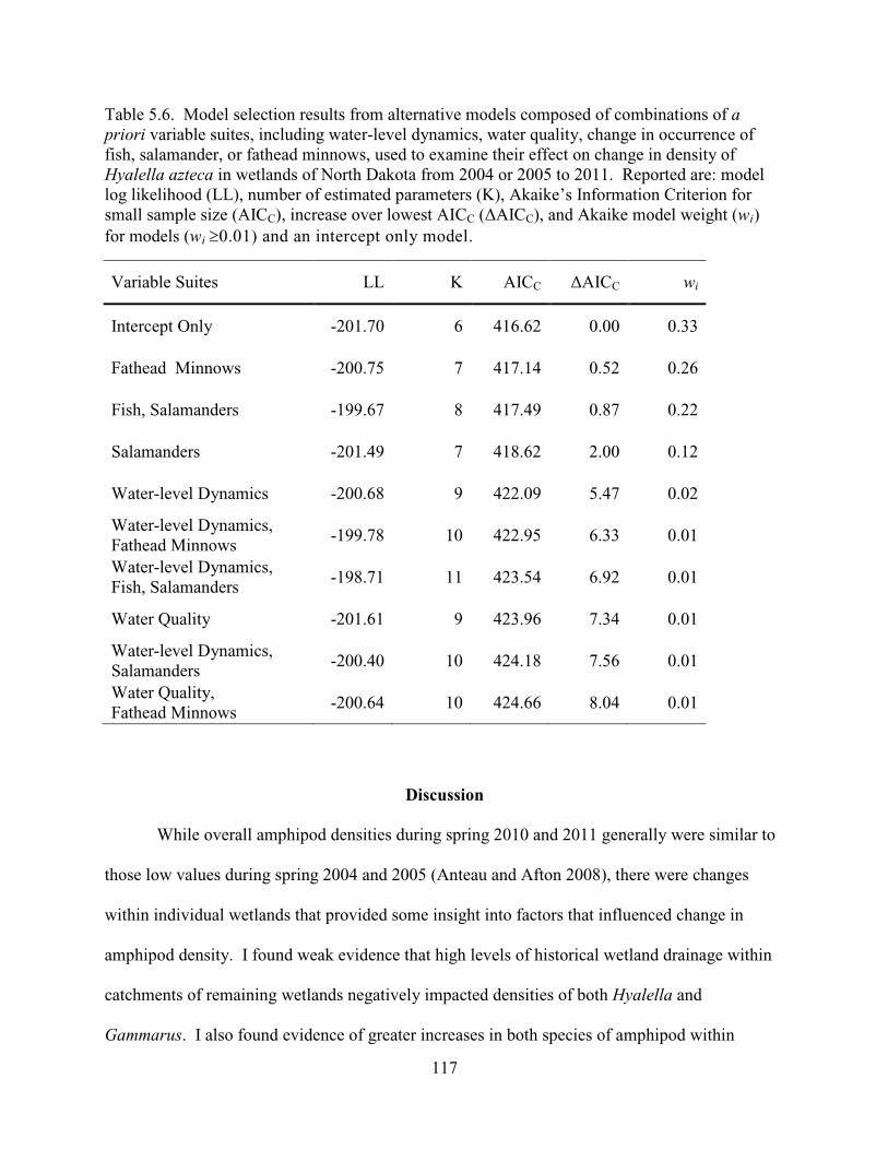
117

Table 5.6. Model selection results from alternative models composed of combinations of a priori variable suites, including water-level dynamics, water quality, change in occurrence of fish, salamander, or fathead minnows, used to examine their effect on change in density of Hyalella azteca in wetlands of North Dakota from 2004 or 2005 to 2011. Reported are: model log likelihood (LL), number of estimated parameters (K), Akaike’s Information Criterion for small sample size (AICC), increase over lowest AICC (∆AICC), and Akaike model weight (wi) for models (wi ≥0.01) and an intercept only model.

Variable Suites LL K AICC ∆AICC wi

Intercept Only -201.70 6 416.62 0.00 0.33

Fathead Minnows -200.75 7 417.14 0.52 0.26

Fish, Salamanders -199.67 8 417.49 0.87 0.22

Salamanders -201.49 7 418.62 2.00 0.12

Water-level Dynamics -200.68 9 422.09 5.47 0.02

Water-level Dynamics, Fathead Minnows

-199.78 10 422.95 6.33 0.01

Water-level Dynamics, Fish, Salamanders

-198.71 11 423.54 6.92 0.01

Water Quality -201.61 9 423.96 7.34 0.01

Water-level Dynamics, Salamanders

-200.40 10 424.18 7.56 0.01

Water Quality, Fathead Minnows

-200.64 10 424.66 8.04 0.01

Discussion

While overall amphipod densities during spring 2010 and 2011 generally were similar to

those low values during spring 2004 and 2005 (Anteau and Afton 2008), there were changes

within individual wetlands that provided some insight into factors that influenced change in

amphipod density. I found weak evidence that high levels of historical wetland drainage within

catchments of remaining wetlands negatively impacted densities of both Hyalella and

Gammarus. I also found evidence of greater increases in both species of amphipod within

118

wetlands that filled more of their topographic basins; this might be related to more-full basins

having or being connected to deeper-water overwintering habitat. However, my data also

suggests that Hyalella were less abundant in wetlands of greater depth. This could be associated

to differences in other Hyalella habitat characteristic that are coincident with greater wetland

depth, such as structure of submerged aquatic vegetation communities, or those wetlands

becoming suitable for fish. However, fish did not appear to be important in explaining changes

in Hyalella densities.

Water levels in wetlands fluctuated in response to wet–dry periods, but the influence of

climate variability on water-level fluctuations differed depending upon the amount of wetland

drainage within the catchment (Chapter 2). Wetlands within catchments with more historical

wetland drainage experienced less drawdown and more flooding than those in less drained

catchments (<2% area drained). However, I did not find evidence of increased amphipod

densities in wetlands where water-level fluctuations occurred whether it be new flooding

terrestrial areas or re-flooding of dried wetland shore. Perhaps there is a more direct negative

influence limiting amphipod densities than are nutrients limiting amphipod densities in these

wetlands.

Amphipods are highly productive and capable of producing multiple broods within a

breeding season (Covich and Thorp 1991; Wen 1992; Pickard and Benke 1996); therefore, it is

unlikely that sampling in 2010 and 2011 was too early after the drawdown to observe a pulse in

productivity of Gammarus and Hyalella in response to cycling of nutrients. Having an R-

selected life history (Pianka 1970), it is likely that amphipod densities would respond to

improved hydrologic and nutrient conditions within the first two years following of the wet

period. Accordingly, I believe my study duration captured the important changes in amphipod

119

densities that can be attributed to the rewetting event of 2009. While mean amphipod densities

were lower in 2010 than in 2011 in some instances, the difference is more likely a result of a

further increase in water levels that increased the number of wetlands suitable habitat for

overwinter survival of amphipods. Indeed, I observed overwinter survival of amphipod

populations of both species in more wetlands in 2011 than in 2010. An increase in wetlands

suitable for overwinter survival can contribute to improved amphipod densities across landscapes

within the region. Perhaps of more importance to waterbird conservation is understanding what

factors limit amphipod productivity within individual wetlands and how some wetlands can

support extremely high densities of amphipods.

Historical estimates of amphipod densities are too sparse to allow for rigorous

quantitative comparisons with current densities. However, Anteau and Afton (2008) concluded

that densities in 2004 and 2005 likely had declined from historical levels based on comparisons

with available amphipod data and marked shifts in lesser scaup diets away from amphipods to

lesser-preferred foods (Anteau and Afton 2006; Strand et al. 2008; Anteau and Afton 2009a) and

concurrent declines in lipid reserves and lipid acquisition of lesser scaup during spring migration

(Anteau and Afton 2004, 2009b, 2011). I quantitatively evaluated our estimates in relation to

those of Anteau and Afton (2008) in North Dakota, and our estimates are similar to those

reported low estimates. Accordingly, my results suggest that the potential decline in amphipod

densities in North Dakota that Anteau and Afton (2008) observed was not driven by the temporal

position between wet–dry periods when data were collected.

During 2010–2011 there were more ideal hydrologic conditions than that during 2004–

2005. I expected wetlands with high water-levels following the dry period in 2006–2008 to

contain greater nutrient concentrations that would benefit wetland productivity. Indeed, I did

120

observe water-level fluctuations during the climatic wet–dry periods in wetlands with less

drainage within their catchment, yet finding little overall change in amphipod density between

sampling periods perhaps suggests either 1) that amphipod densities are now less tied to temporal

position in climate wet–dry fluctuations than they were previously or 2) amphipods are not as

responsive to climate as predicted. Although extremes of climate conditions that occur across

decades likely do effect amphipod populations by temporarily reducing available suitable habitat,

long-term declines in amphipod density across the region are more likely a result of landscape

modifications that affect wetland hydrology, increased sedimentation, eutrophication, and

increased agrochemical residues entering wetlands (Grue et al. 1988; Gleason and Euliss 1998;

Anteau et al. 2011). Thus availability of suitable habitat for amphipods in lacustrine wetlands

may be more-permanently reduced.

Literature Cited



Anteau, M. J., and A. D. Afton. 2004. Nutrient reserves of lesser scaup (Aythya affinis) during

spring migration in the Mississippi flyway: a test of the spring condition hypothesis. Auk

121:917–929.





Anteau, M. J., and A. D. Afton. 2009a. Wetland use and feeding by lesser scaup during spring


121

Anteau, M. J., and A. D. Afton. 2009b. Lipid reserves of lesser scaup (Aythya affinis) migrating

across a large landscape are consistent with the “spring condition” hypothesis. Auk

126:873–883.






Balas, C., N. Euliss, Jr., and D. Mushet. 2012. Influence of conservation programs on

amphibians using seasonal wetlands in the Prairie Pothole Region. Wetlands 32:333–345.

Bartzen, B. A., K. W. Dufour, R. G. Clark, and F. D. Caswell. 2010. Trends in agricultural

impact and recovery of wetlands in prairie Canada. Ecological Applications 20:525–538.






Benoy, G. A. 2005. Variation in tiger salamander density within prairie potholes affects aquatic

bird foraging behaviour. Canadian Journal of Zoology 83:926–934.



York, NY, USA.

122

Castelle, A. J., A. W. Johnson, and C. Conolly. 1994. Wetland and stream buffer size

requirements—a review. Journal of Environmental Quality 23:878–882.

Covich, A. P., and J. H. Thorp. 1991. Crustacea: introduction and peracardia. In J. H. Thorp, and

A. P. Covich (eds) Ecology and classification of North American freshwater

invertebrates. Academic Press, San Diego, California, USA, pp 665–689.






Devore, J. L. 2000. Probability and statistics for engineering and the sciences. Duxbury, Pacific

Grove, CA, USA.

Duan, Y., S. I. Guttman, J. T. Oris, and A. J. Bailer. 2000. Genotype and toxicity relationships

among Hyalella azteca: I. acute exposure to metals or low pH. Environmental Toxicology

and Chemistry 19:1414–1421.




458.

123





514.








Hanson, M. A., and M. G. Butler. 1994. Responses to food web manipulation in a shallow

waterfowl lake. Hydrobiologia 279-280:457–466.




Hentges, V. A., and T. W. Stewart. 2010. Macroinvertebrate assemblages in Iowa Prairie Pothole

wetlands and relation to environmental features. Wetlands 30:501–511.




124




Lindeman, D., and R. Clark. 1999. Amphipods, land-use impacts, and lesser scaup (Aythya

affinis) distribution in Saskatchewan wetlands. Wetlands 19:627–638.

Macneil, C., J. T. A. Dick, and R. W. Elwood. 1999. The dynamics of predation on Gammarus

spp. (Crustacea: Amphipoda). Biological Reviews 74:375–395.





Wetlands 34:1123–1132.

Mushet, D. M., J. L. Neau, and N. H. Euliss Jr. 2014. Modeling effects of conservation grassland

losses on amphibian habitat. Biological Conservation 174:93–100.

Nakagawa, S., and H. Schielzeth. 2013. A general and simple method for obtaining R2 from

generalized linear mixed-effects models. Methods in Ecology and Evolution 4:133–142.

National Climate Data Center (NCDC). 2014. Time bias corrected divisional temperature,

precipitation, and drought index.

http://www7.ncdc.noaa.gov/CDO/CDODivisionalSelect.jsp - accessed: 1/24/2014.

Nyman, J. A., and R. H. Chabreck. 1996. Some effects of 30 years of weir-management on

coastal march aquatic vegetation and implications for waterfowl management. Gulf of

Mexico Science 14:16–25.

125

Olenick, R. J., and J. H. Glee. 1981. Tiger salamanders (Ambystoma tigrinum) and stocked

rainbow trout (Salmo gairdneri): potential competitors for food in Manitoba prairie

pothole lakes. Canadian Field-Naturalist 95:129–132.

Pianka, E. R. 1970. On r- and K-Selection. American Naturalist 104:592–597.

Pickard, D. P., and A. C. Benke. 1996. Production Dynamics of Hyalella azteca (Amphipoda)

among Different Habitats in a Small Wetland in the Southeastern USA. Journal of the

North American Benthological Society 15:537–550.





Strand, K., S. Chipps, S. Kahara, K. Higgins, and S. Vaa. 2008. Patterns of prey use by lesser

scaup Aythya affinis (Aves) and diet overlap with fishes during spring migration.








USA, pp 565–576.



126

Wen, Y. H. 1992. Life history of Hyalella azteca (Crustacea:Amphipoda) in a hypereutrophic

prairie pond in southern Alberta. Canadian Journal of Zoology 70:1417–1424.

Zimmer, K. D., M. A. Hanson, and M. G. Butler. 2000. Factors influencing invertebrate

communities in prairie wetlands: a multivariate approach. Canadian Journal of Fisheries


127

CHAPTER 6. A LANDSCAPE-SCALE EVALUATION OF THE “ALTERNATIVE

STABLE STATE” HYPOTHESIS WITHIN LARGE NORTHERN PRAIRIE

WETLANDS IN CONTEXT OF WATERBIRD CONSERVATION

Abstract

Trophic structure of wetlands can be a useful indicator of their biological productivity,

biodiversity, and overall perceived quality. The “alternative stable states” hypothesis suggests

ecosystems can exist in discrete alternative trophic structures. In wetlands, alternative states

include a clear state where primary productivity is dominated by macrophytes and a turbid state

where primary productivity is dominated by phytoplankton. Chlorophyll a (chl a) concentration

in water is commonly used to indicate trophic structure in wetlands because it is a key pigment in

phytoplankton. I conducted a landscape-scale evaluation of the alternative stable state

hypothesis by examining the distribution of remotely-sensed chl a concentrations during 2011

within 978 randomly selected semipermanent and permanent wetlands in the Prairie Pothole

Region of North Dakota. Under the alternative stable states hypothesis I predicted that two

alternative states should be observable as a bimodal distribution in a large sample of wetlands.

Additionally, I evaluated how wetland chl a concentrations were related to consolidation

drainage, upland land use, and fish abundance. The distribution of wetland mean chl a

concentrations was unimodal, skewed right, and lacked evidence of discontinuity. Chl a

concentration was positively correlated with the percent of the wetland basin filled by surface

water (β� = 0.0090 ±0.0018 SE) and negatively correlated with the percent of surrounding upland

that was grassland (β� = -0.6415 ±0.1993 SE). My evaluation did not support predictions of the

alternative stable state hypothesis. Rather, my data suggest that these wetlands behave in a

continuum of trophic structure, and that manifestation of trophic structure is influenced by a

128

continuum of perturbations. Accordingly, for the purposes of improving conservation planning,

my findings suggest that a continuous model would be more useful than characterizing wetlands

within the framework of “alternative stable states”.

Introduction

Anthropogenic modifications within wetland landscapes can potentially have catastrophic

effects on wetland trophic structure—an important construct of relationships that can be used to

index biological productivity, biodiversity, and other services provided by wetlands.

Modifications that alter hydrology, nutrient cycling, vegetation communities, and allow for fish

to persist may lead to less desirable trophic structures within wetlands (Hanson and Butler

1994a; Carpenter et al. 1998; Sánchez-Carrillo and Álvarez-Cobelas 2001; Chapters 2–4).

Chemical, physical, and biologic characteristics are often used as indicators of trophic structure

in wetlands and ultimately as a measure of wetland productivity (Carlson 1977; Grue et al. 1988;

Tome et al. 1995; Anteau and Afton 2008; Anteau et al. 2011). Accordingly, the capability to

make landscape-scale assessments of wetland trophic structure may prove useful for managers to

better assess wetland condition and understand influences of land use practices on that wetland

condition.

Scheffer et al. (1993) proposed that there are two alternative stable states for shallow

lakes (<3 m depth; hereafter wetlands), a clear state where primary productivity is dominated by

macrophytes and a turbid state where primary productivity is dominated by phytoplankton

(hereafter the “alternative stable states” hypothesis). Later, Scheffer and van Nes (2007)

acknowledged various alternative states in temperate wetlands that are alternatively dominated

by primary producers including: charophytes, submerged angiosperms, green algae, or

cyanobacteria. However, the alternative stable states hypothesis maintains that there is

129

discontinuity in wetland community responses to environmental changes resulting in alternative

equilibria producing multiple distinguishable trophic states (Scheffer and van Nes 2007). Within

the core example of alternative stable states, macrophyte-dominated communities have food

webs with higher density and diversity of invertebrates and vertebrates than those of

phytoplankton-dominated wetlands (Hargeby et al. 1994; Scheffer and van Nes 2007).

Consequently, clear-water wetlands generally provide more food and better foraging efficiency

for waterbirds than do those dominated by phytoplankton (Anteau and Afton 2008, 2009).

Abundance of clear-water wetlands with high productivity of aquatic macroinvertebrates are

important habitat for many waterbirds that breed locally in the Prairie Pothole Region and for

those migrating through to breed elsewhere (Batt et al. 1989; Swanson and Duebbert 1989;

Anteau and Afton 2006, 2011).

According to the alternative stable state hypothesis, alternate states are shaped by

stabilizing feedback mechanisms within wetland communities (Scheffer 2001). In clear-water

wetlands, submerged aquatic vegetation can maintain a clear state by 1) reducing resuspension of

sediments (Dieter 1990; James and Barko 1990); 2) suppressing phytoplankton through

reduction of available nutrients and releasing allelochemicals; and 3) providing refuge for

phytoplankton-grazing zooplankton and habitat for alternative prey for predators of

phytoplankton-grazing zooplankton (Timms and Moss 1984; Scheffer et al. 1993; Hanson and

Butler 1994a). In turbid-water wetlands, submerged vegetation growth is prevented by

obstruction of light from high phytoplankton densities or suspended sediments (Scheffer et al.

1993). Further, fish can increase turbidity of wetlands by resuspending sediments and by

preying upon zooplankton that consume phytoplankton, with cascading effects on the community

of submerged vegetation and macroinvertebrates dependent on that vegetation for habitat

130

(Swanson and Nelson 1970; Timms and Moss 1984; Carpenter et al. 1985; Scheffer et al. 1993;

Hanson and Butler 1994a, b; Zimmer et al. 2003). Communities in each state can resist against

some degree of perturbation within the wetland basin or catchment, such as increased

sedimentation, nutrification, change in fish density, water-level fluctuation, or climate variation

(Scheffer et al. 1993; Hanson and Butler 1994a; Gunderson and Pritchard 2002; Bayley et al.

2007). However, beyond some threshold, a catastrophic regime shift may occur as the wetland

enters an alternative stable state (Scheffer et al. 1993; Scheffer 2001) with consequences that

affect productivity, species density, and species richness (Holling 1973; May 1977; Scheffer et

al. 2001; Folke et al. 2004).

Chlorophyll a (chl a) concentrations are typically used as a proximate estimator of

biomass of phytoplankton in aquatic systems (e.g., Carlson 1977; Scheffer et al. 1997; Bayley

and Prather 2003; Zimmer et al. 2009). Previous investigations have used chl a concentration to

differentiate clear from turbid wetlands in the Prairie Pothole Region of Minnesota (Zimmer et

al. 2009) and in boreal wetlands of Alberta (Bayley and Prather 2003). The alternative stable

states hypothesis postulates that wetlands can be characterized by either clear or turbid states,

thus I predict that for this hypothesis to be supported wetland chl a concentrations should follow

a bimodal distribution across the region. Further, evaluation of the frequency of turbid wetlands

in various landscape conditions may provide insight into levels of disturbance that have potential

to cause a regime shift. That information could be used to focus conservation or restoration

efforts on wetlands that are sensitive to a regime shift.

Remote sensing-techniques used to estimate chl a concentrations make it possible to

conduct landscape-scale assessment of wetland trophic structure. Successful estimation of chl a

concentrations using Landsat Thematic Mapper (TM) and Enhanced Thematic Mapper Plus

131

(ETM+) imagery have been made in deep, large lakes and reservoirs (Brivio et al. 2001; Cheng

and Lei 2001), and in shallow, smaller lakes (Tyler et al. 2006; Sass et al. 2007). Use of remote

sensing techniques adapted for estimation of chl a in prairie wetlands can allow for a large

enough sample of wetlands required to adequately evaluate the prediction of the alternative

stable state hypothesis.

I evaluated the alternative stable state hypothesis within wetlands in the Prairie Pothole

Region of North Dakota. To conduct a landscape-scale evaluation of the distribution of clear and

turbid wetlands, I developed remote sensing techniques of chl a concentrations for larger

semipermanent and shallow-water permanent wetlands. I remotely-sensed chl a concentrations

in a large sample of wetlands and evaluated the distribution for evidence of bimodality that

would support the prediction of alternative discrete states. I also evaluated if anthropogenic

modifications within wetland catchments had a negative impact on wetland trophic structure by

increasing chl a concentrations. I evaluated whether these land use and upland modification

effects better predicted the probability of a wetland being turbid within a binomial model or

alternatively, wetland chl a concentrations within a continuous model.

Methods

Study Area

I focused my effort to adapt remote sensing predictive methods for detection of chl a

concentration and evaluation of the alternative stable states hypothesis on large (>10 ha)

semipermanent and shallow-water permanent wetlands within the Prairie Pothole Region in

North Dakota (Figure 6.1). I used a sample of 153 lacustrine semipermanent and shallow-water

permanent wetlands that were previously randomly selected for purposes of a previous study

(Anteau and Afton 2008; Chapter 2–5). These wetlands were known from the previous studies

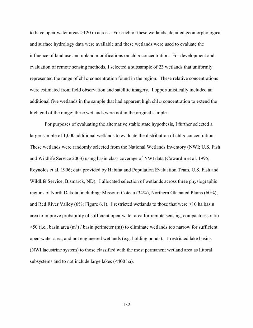
132

to have open-water areas >120 m across. For each of these wetlands, detailed geomorphological

and surface hydrology data were available and these wetlands were used to evaluate the

influence of land use and upland modifications on chl a concentration. For development and

evaluation of remote sensing methods, I selected a subsample of 23 wetlands that uniformly

represented the range of chl a concentration found in the region. These relative concentrations

were estimated from field observation and satellite imagery. I opportunistically included an

additional five wetlands in the sample that had apparent high chl a concentration to extend the

high end of the range; these wetlands were not in the original sample.

For purposes of evaluating the alternative stable state hypothesis, I further selected a

larger sample of 1,000 additional wetlands to evaluate the distribution of chl a concentration.

These wetlands were randomly selected from the National Wetlands Inventory (NWI; U.S. Fish

and Wildlife Service 2003) using basin class coverage of NWI data (Cowardin et al. 1995;

Reynolds et al. 1996; data provided by Habitat and Population Evaluation Team, U.S. Fish and

Wildlife Service, Bismarck, ND). I allocated selection of wetlands across three physiographic

regions of North Dakota, including: Missouri Coteau (34%), Northern Glaciated Plains (60%),

and Red River Valley (6%; Figure 6.1). I restricted wetlands to those that were >10 ha basin

area to improve probability of sufficient open-water area for remote sensing, compactness ratio

>50 (i.e., basin area (m2) / basin perimeter (m)) to eliminate wetlands too narrow for sufficient

open-water area, and not engineered wetlands (e.g. holding ponds). I restricted lake basins

(NWI lacustrine system) to those classified with the most permanent wetland area as littoral

subsystems and to not include large lakes (<400 ha).

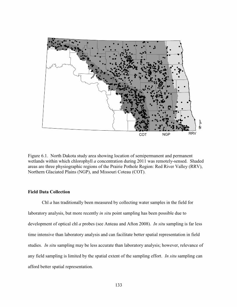
133

Figure 6.1. North Dakota study area showing location of semipermanent and permanent wetlands within which chlorophyll a concentration during 2011 was remotely-sensed. Shaded areas are three physiographic regions of the Prairie Pothole Region: Red River Valley (RRV), Northern Glaciated Plains (NGP), and Missouri Coteau (COT).

Field Data Collection

Chl a has traditionally been measured by collecting water samples in the field for

laboratory analysis, but more recently in situ point sampling has been possible due to

development of optical chl a probes (see Anteau and Afton 2008). In situ sampling is far less

time intensive than laboratory analysis and can facilitate better spatial representation in field

studies. In situ sampling may be less accurate than laboratory analysis; however, relevance of

any field sampling is limited by the spatial extent of the sampling effort. In situ sampling can

afford better spatial representation.

134

During late June through early September in 2011 or 2012, I measured chl a

concentrations in 28 different wetlands using in situ sonde point sample measurements and

collecting water samples for laboratory fluorometry. I expected chl a concentration to peak

during this period of the summer, thus providing the widest range of chl a concentration.

Estimation of phytoplankton biomass using chl a concentration is sensitive time of day (APHA

1998); therefore, I timed field measurements to correspond to the same time of day as Landsat

satellite imagery acquisitions, approximately 10:00–14:00 CDT, and only on mostly cloud-free

days no more than two days after a generally cloud-free acquisition of Landsat image. I also

limited data collection to days with calm winds. I used a small boat to make measurements and

collect water samples within wetlands.

In situ measurements and collected water samples were taken from open-water areas in

wetlands (>30 m of open water in each direction) within 30×30 m sampling frames that were

spatially aligned with pixels from either the previous TM/ETM+ image if sampling on the same

day as image acquisition, or the image of interest when sampling after image acquisition. I

sampled 15–25 sampling frames within each wetland, or all frames if < 25 were available.

Sampling frames were arranged in clusters of five adjacent frames, and clusters were distributed

to different areas within the wetland. Within each frame, I recorded in situ point measurements

approximately at the center and 10–12 m from center in three directions (n = 4); each point

sample consisted of 10 measurements collected at 1 second intervals. I collected one water

sample in smaller wetlands or two samples in larger wetlands, each at the center of a sampling

frame. All in situ measurements and water samples were georeferenced using a Trimble GeoXT

(differential correction; Trimble Navigation, Sunnyvale, CA).

135

I used YSI 6025 chlorophyll probe and YSI 6136 turbidity probe (YSI Incorporated,

Yellow Springs, Ohio) for in situ measurements at each sample point. At the beginning of each

sampling day, I calibrated the chlorophyll probe to a zero measurement using distilled water. I

also recorded measurements in 0.5 mg/L Rhoadamine WT at the beginning and end of each

sampling day to check for sensor drift. I calibrated the turbidity probe once at the beginning of

each season. I aggregated multiple readings from each point sample and the four point samples

within the sampling frame to calculate a median value for chlorophyll and turbidity. Use of the

median (rather than the mean) value better controls for erroneous readings that occur periodically

in electronic-probe measurements.

I collected water samples that corresponded directly to the georeferenced in situ location

to enable post-calibration of the probe using results from laboratory fluorometric analysis of chl

a. Each water sample consisted of 1 L of water collected just below the surface. Water samples

were filtered through a glass fiber filter (45 µm, 47 mm diameter). Filters were immediately

frozen for fluorometry analysis (APHA 1998) within 10 days of collection. Laboratory analysis

was performed by North Dakota Department of Health’s Surface Water Quality Management

Program. I used regression analysis without an intercept to calibrate in situ chl a measurements

to laboratory fluorometry results.

Landsat Data

I obtained Landsat 5 TM and Landsat 7 ETM+ product level 1T precision and terrain

corrected images from Earth Explorer (U.S. Geological Survey 2014). A total of 19 images of

the study area were used from scenes within path 29–35 and row 26–28 of the Worldwide

Reference System 2 (Table 6.1). All images used were <12% cloud cover, with the exception of

two images with 18% and 45% cloud cover from which only cloud-free portions of the image

136

were used to correspond to cloud-free field data collection. I converted image digital numbers to

top-of-atmospheric reflectance using at-sensor values (Chander et al. 2009), and then I used the

Automated Cloud-Cover Assessment algorithm to detected and masked clouds (Irish et al. 2006).

I corrected images for atmospheric effects using the 6S algorithm (Vermote et al. 1997) with

optical depth from the Moderate Resolution Imaging Spectroradiometer (MODIS) Level 3 Daily

Atmosphere Gridded Product (NASA 2014). For each scene, I calculated the optical depth as the

scene average of mean optical land and ocean values from the MODIS product.

I extracted reflectance values (R) for TM/ETM+ bands 1–5 and 7 (Table 6.2) from pixels

that corresponded to in situ measurement sample frames or open-water pixels from the 1,000

wetlands. I used images acquired between 3 July and 5 September of 2011 with preference for

cloud-free images nearest 19 July (ordinal day 200). To select open-water pixels within the

1,000 randomly selected wetlands, I initially offset (i.e., buffered) the perimeter of the NWI

basin class coverage polygon 60 m toward the center of the wetland. I then applied a series of

filters to eliminate pixels that were not registering as open-water using band 5 (RB5 > 0.03),

registering apparent emergent or submerged vegetation (RB4 / RB2 ≥ 2), or had a signature of a

hypersaline turbid water wetland (RB1 > 0.05). Hypersaline wetlands were excluded from this

analysis because their water quality condition is beyond the scope of this analysis, and their

overall brightness within the spectral signature present problems remotely-sensing a chl a

signature. From the initial 153 wetland sample combined with the additional 1,000 randomly

selected wetlands, 978 wetlands were suitable for remote sensing of chl a concentration after

open-water pixel filters were applied (>1 open-water pixel).

137

Table 6.1. Landsat Thematic Mapper (TM) and Enhanced Thematic Mapper Plus (ETM+) scenes used to build and evaluate a predictive model of Chlorophyll a concentration in wetlands (Model) and to make predictions within wetlands in a landscape-scale assessment (Predict). Listed are the Landsat Scene Identifier, year of image (Year), ordinal day of year (Day), World Reference System 2 scene (Row and Path), and optical sensor that acquire the image (Sensor).

Scene Identifier Year Day Path Row Sensor Model Predict

LT50330262011184PAC01 2011 184 33 26 TM Yes No

LT50330272011184PAC01 2011 184 33 27 TM Yes Yes

LT50310272011186PAC01 2011 186 31 27 TM Yes Yes

LT50310282011186PAC01 2011 186 31 28 TM No Yes

LT50320262011193PAC01 2011 193 32 26 TM No Yes

LT50320272011193PAC01 2011 193 32 27 TM Yes Yes

LT50310262011202PAC01 2011 202 31 26 TM No Yes

LT50300262011211PAC01 2011 211 30 26 TM No Yes

LT50300272011211PAC01 2011 211 30 27 TM Yes Yes

LT50300282011211PAC01 2011 211 30 28 TM No Yes

LT50320262011225PAC01 2011 225 32 26 TM No Yes

LT50350262011230PAC01 2011 230 35 26 TM No Yes

LT50290282011236PAC03 2011 236 29 28 TM No Yes

LT50340262011239PAC01 2011 239 34 26 TM No Yes

LT50330262011248PAC01 2011 248 33 26 TM No Yes

LE70300282012174EDC00 2012 174 30 28 ETM+ Yes No

LE70300282012190EDC00 2012 190 30 28 ETM+ Yes No

LE70300272012222EDC00 2012 222 30 27 ETM+ Yes No

LE70310282012229EDC00 2012 229 31 28 ETM+ Yes No

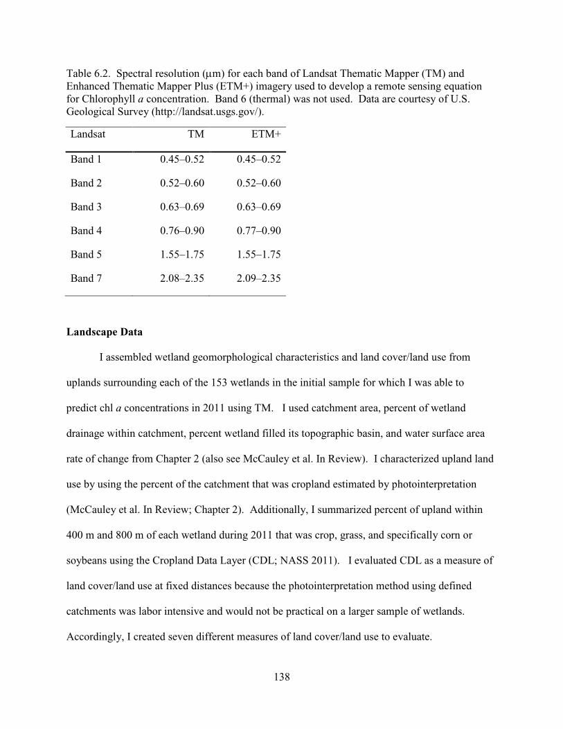
138

Table 6.2. Spectral resolution (µm) for each band of Landsat Thematic Mapper (TM) and Enhanced Thematic Mapper Plus (ETM+) imagery used to develop a remote sensing equation for Chlorophyll a concentration. Band 6 (thermal) was not used. Data are courtesy of U.S. Geological Survey (http://landsat.usgs.gov/).

Landsat TM ETM+

Band 1 0.45–0.52 0.45–0.52

Band 2 0.52–0.60 0.52–0.60

Band 3 0.63–0.69 0.63–0.69

Band 4 0.76–0.90 0.77–0.90

Band 5 1.55–1.75 1.55–1.75

Band 7 2.08–2.35 2.09–2.35

Landscape Data

I assembled wetland geomorphological characteristics and land cover/land use from

uplands surrounding each of the 153 wetlands in the initial sample for which I was able to

predict chl a concentrations in 2011 using TM. I used catchment area, percent of wetland

drainage within catchment, percent wetland filled its topographic basin, and water surface area

rate of change from Chapter 2 (also see McCauley et al. In Review). I characterized upland land

use by using the percent of the catchment that was cropland estimated by photointerpretation

(McCauley et al. In Review; Chapter 2). Additionally, I summarized percent of upland within

400 m and 800 m of each wetland during 2011 that was crop, grass, and specifically corn or

soybeans using the Cropland Data Layer (CDL; NASS 2011). I evaluated CDL as a measure of

land cover/land use at fixed distances because the photointerpretation method using defined

catchments was labor intensive and would not be practical on a larger sample of wetlands.

Accordingly, I created seven different measures of land cover/land use to evaluate.

139

Wetland Surface Area Dynamics

I included water dynamics in my analysis evaluating influence of land use and upland

modifications on wetland chl a concentrations because vegetation communities can be

influenced by wetland water dynamics (Weller and Spatcher 1965; van der Valk and Davis

1978). In Chapter 2, I defined wetland water surface area dynamics within the variable climate

conditions during 2003–2010 in terms of rate of decrease during a drying phase and rate of

increase during a wetting phase. I calculated these rates using the maximum surface area during

the wet periods and minimum surface are during the dry period within the equation:

� Surface Area��Surface Area��

Statistical Analysis

Post-calibration of in situ chlorophyll a

I tested the importance of turbidity within the regression model as a covariate to account

for potential differences between in situ and filtered laboratory samples. I evaluated collinearity

between chl ain situ and turbidity using variance inflation factor (vif = 2.31). I used the final

regression equation to calculate post-calibrate chl a (chl apc) values for all in situ measurements

(R Development Core Team 2010).

Landsat to predict in situ chlorophyll a

For development of a model to predict wetland chl a concentration using TM/ETM+ data

I used in situ sampling frames corresponding to image pixels as the observational unit. I

randomly split in situ sampling frames into two halves equal in number to create a model

development data set and a model evaluation data set. I split sampling frames into development

and evaluation groups rather than individual wetlands because I was only able to sample 26

wetlands. I evaluated previously published (see list in Sass et al. 2007) and new combinations of

140

single bands, multiple band combinations, and principal components of visual spectrum bands

(1–3) and all non-thermal bands (1–5, 7) in regression analysis as predictor variables of chl apc

(ln) . I excluded predictor variables with strong collinearity (r ≥ 0.40) to others in the same

model. I used 95% confidence intervals to evaluate importance of predictor variables and model

R2 values to compare goodness-of-fit among models and to select the best model for making

predictions. I then used the best model to make predictions (chl ars) within in situ sampling

frames from the evaluation data set. I evaluated regression coefficients and correlation to

determine adequacy of chl ars as a predictor of chl apc. Finally, I evaluated prediction

performance at a wetland resolution by regressing wetland mean chl apc on wetland mean chl ars.

Landscape distribution of wetland chlorophyll a concentration

I used the chl ars predictive equation to estimate chl a concentration in 978 randomly

selected wetlands at one point in time during 2011. I applied the equation to open-water pixels

from TM images, and then calculated the wetland mean chl ars. I evaluated whether the

distribution of chl a concentrations in wetlands supported the alternative stable states hypothesis

by plotting a histogram of wetland mean chl ars concentrations. Interpretation of distributions by

categorical frequency is sensitive to selection of category break points and bin ranges. Clearly,

to evaluate bimodality a uniform bin size is needed. I used 5 µg L-1 bins to represent wetland chl

a concentrations. A distinct bimodal distribution would support predictions made under the

hypothesis of clear and turbid wetlands, measurable by chl a.

Landscape factors influencing chlorophyll a concentration

I quantitatively assessed two models for evaluating influences of land use and upland

modifications on trophic structure. The first was an alternative stable state model that examined

the probability of a wetland being in a turbid or clear state (as defined by Bayley and Prather

141

2003; Zimmer et al. 2009) using a binomial distribution. Second, represented an alternative

research hypothesis where trophic status changes continuously with changes in landscape

variables. For that model a continuous distribution of wetland chl a concentration was used. In

the prediction following the alternative stable state hypothesis, landscape variables should better

predict the probability of a wetland being turbid within a binomial distribution than would

landscape variables predict wetland chl a concentration within a continuous distribution. Within

the initial sample of wetlands for which detailed geomorphological and surface hydrology data

were available, 117 wetlands were suitable for remote sensing of chl a. I used chl ars derived

from TM data collected in 2011 as the response variable in continuous regression analysis and

classified chl ars >20 µg L-1 as a turbid wetland in logistic regression analysis (R Development

Core Team 2010). For each analysis I used the same a priori model that included land use and

upland modification predictor variables from wetland for which I had detailed geomorphological

and surface hydrology data. Predictors included: wetland basin percent full, percent catchment

area that was drained wetland, catchment area (ln), water surface area dynamics, and land

cover/land use. Prior to fitting my a priori model, evaluated drying rate versus wetting rate as a

measure of water surface area and seven different measures of land use/land cover by iteratively

fitting each one with all other predictor variables of the a priori model. I repeated this process

for both the binomial and continuous models. I selected the model with the greatest R2. I

determined predictor variables to be important in the model if 95% confidence intervals of

parameter estimates did not overlap zero. I plotted fitted values versus response values for both

the binomial model and continuous model (one point omitted at [21,132]). I compared R2 to

evaluate which model distribution was better supported by my data.

142

Results

Post-Calibration of In Situ Chlorophyll a

I recorded 1876 in situ point samples and collected 45 water samples within 28 wetlands.

In situ chl a measurements predicted laboratory fluorometry values well (R2 = 0.93, F2, 43 =

284.9) provided that the level of turbidity was in the model:

Chl �� 0.47#$0.18 SE()Chl �*+ ,*-./ 0 2.90 #$0.21 SE()turbidity/

Landsat to Predict In Situ Chlorophyll a

The best models to predict chl a concentration in wetlands using TM and ETM+ were:

�8Chl �9: ;<= � 6.70 0 9.27 ? RAB C RAD C RAE�RAB 0 RAD 0 RAE

F C 0.74 ?GRAHIJF

�8Chl �9: K;<L= � 6.87 0 17.95 ? RAB C RAD C RAE�RAB 0 RAD 0 RAE

F C 0.74 ?GRAHIJF

Each parameter in the model was important for prediction (Table 6.3). Chl ars described 72%

(R2; F4, 311 = 197.2) of the variability within in situ chl apc values. In the evaluation data set, chl

ars predicted in situ chl apc values with an intercept of 3.970 (SE = 3.353) and slope of 1.269(SE

= 0.048), with an R2 of 69% (F1, 314 = 693.9). Aggregated mean chl ars and in situ chl apc values

in 26 wetlands were highly correlated (r = 0.93, t = 3.733, df = 24, P = 0.005; Figure 6.2).

Landscape Distribution of Wetland Chlorophyll a Concentration

Chl ars ranged 3–714 µg L-1, with a mean of 27 µg L-1 and median of 17 µg L-1. The

distribution of wetland mean chl a concentration was skewed right (Figure 6.3), and no evidence

of bimodality was present in a histogram of truncated at 100 µg chl a L-1 (Figure 6.4).

Landscape Factors Influencing Chlorophyll a Concentration

Chl ars ranged 4–133 µg L-1, with a mean of 19 µg L-1 and median of 15 µg L-1. In the a

priori model describing the influence of land use and upland modifications on wetland chl a

143

concentration the measures that best fit the data, for those parameters that had multiple measures,

were rate of water surface area rate of decrease during the drying phase and CDL derived percent

grassland within 400 m of the wetland (Table 6.4). These two predictor variables were used in

addition to wetland basin percent full, percent catchment area that was drained wetland, and

wetland catchment area (ln). The binomial model with the same variables was ranked second

best, but model fit was essentially not different from the top ranked model (Table 6.4). The

continuous model accounted for nearly twice the amount of variability in trophic structure (R2 =

0.32, F5, 111 = 10.61; Figure 6.5A) than the binomial model (R2 = 0.19, χ2df=5 = 26.33; Figure

6.5B). Wetland basin percent full was positively correlated with chl a concentration, and percent

upland that was grassland was negatively correlated with chl a concentration (Table 6.5). There

was not sufficient evidence for correlation of any of the other predictor variables with chl a

concentration (Table 6.5).

Table 6.3. Regression parameter estimates from a model developed to detect chlorophyll a concentrations (ln) within semipermanent and permanent wetlands using Landsat Thematic Mapper (TM) and Enhanced Thematic Mapper Plus image data. Included are: estimated coefficients (β�), standard errors (SE), and lower (LCL) and upper (UCL) 95% confidence limits. At-surface-reflectance values corrected for atmospheric effects (R band #) were used to develop the model. Predictor X1 = (R3 – R5 – R7) / (R3 + R5 + R7)

0.5 and X2 = R4-0.5. A colon indicates an

interaction predictor term.

Predictor β� SE LCL UCL

Intercept 6.869 0.193 6.491 7.247

X1 17.948 1.493 15.022 20.873

X2 -0.740 0.032 -0.803 -0.676

Sensor TM -0.174 0.081 -0.334 -0.015

X1:Sensor TM -8.675 1.627 -11.863 -5.486

144

Figure 6.2. Accuracy evaluation of remotely-sensed chlorophyll a concentrations to predict mean in situ measurements within 26 semipermanent and permanent wetlands in North Dakota.

0 50 100 150 200 250 300

050

100

150

200

250

300

Remotely-Sensed Chlorophyll-a (µg/L)

In S

itu M

easu

red

Chl

orop

hyll-

-a (µ

g/L)

Intercept = -9.17 ± 8.00 SE

Slope = 1.56 ± 0.13 SE

R2 = 0.86

145

Figure 6.3. Natural log distribution of remotely-sensed chlorophyll a concentrations within 978 randomly selected semipermanent and permanent wetlands in North Dakota.

Natural Log Chlorophyll-a (µg L-1)

Per

cent

of W

etla

nds

1 2 3 4 5 6

05

1015

2025

30

146

Figure 6.4. Distribution of remotely-sensed chlorophyll a concentrations within 965 of 978 randomly selected semipermanent and permanent wetlands in North Dakota. Histogram truncated at 100 µg L-1.

Chlorophyll-a (µg L-1)

Per

cent

of W

etla

nds

0 10 20 30 40 50 60 70 80 90 100

05

1015

20

147

Table 6.4. Comparison of coefficient of determination (R2) from regression analysis of two alternative a priori models used to evaluate the influence of land use and upland modifications on probability of a wetland being in a turbid state using a binomial distribution (Model 1) or concentration of Chlorophyll a within wetlands using a continuous distribution (Model 2). Water surface area change during alternative climatic phases (Phase) and measures of land use/land cover (LU/LC) were used in addition to wetland basin percent full, percent catchment area that was drained wetland, and wetland catchment area (ln). See text for details.

Phase LU/LC Model 1: R2 Model 2: R2

Drying Grassland: 400 m 0.201 0.323

Drying Grassland: 800 m 0.195 0.322

Wetting Grassland: 400 m 0.205 0.320

Wetting Grassland: 800 m 0.200 0.319

Drying Cropland: 400 m 0.166 0.272

Drying Cropland: 800 m 0.160 0.268

Wetting Cropland: 400 m 0.168 0.265

Drying Corn & Soy: 800 m 0.147 0.262

Drying Corn & Soy: 400 m 0.148 0.262

Drying Cropland: Catchment 0.145 0.262

Wetting Cropland: 800 m 0.162 0.260

Wetting Corn & Soy: 800 m 0.147 0.253

Wetting Corn & Soy: 400 m 0.148 0.252

Wetting Cropland: Catchment 0.143 0.249

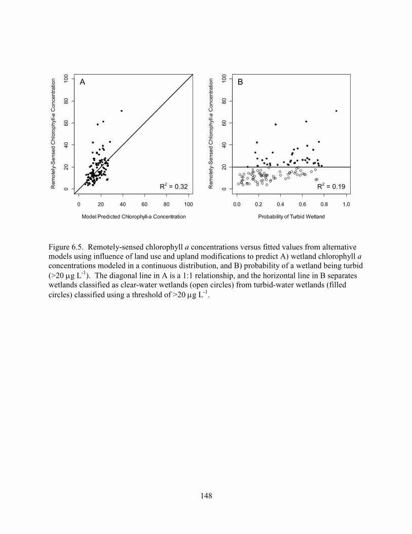
148

Figure 6.5. Remotely-sensed chlorophyll a concentrations versus fitted values from alternative models using influence of land use and upland modifications to predict A) wetland chlorophyll a concentrations modeled in a continuous distribution, and B) probability of a wetland being turbid (>20 µg L-1). The diagonal line in A is a 1:1 relationship, and the horizontal line in B separates wetlands classified as clear-water wetlands (open circles) from turbid-water wetlands (filled circles) classified using a threshold of >20 µg L-1.

0 20 40 60 80 100

020

4060

8010

0

Model Predicted Chlorophyll-a Concentration

Rem

otel

y-S

ense

d C

hlor

ophy

ll- a C

once

ntra

tion

0.0 0.2 0.4 0.6 0.8 1.0

020

4060

8010

0Probability of Turbid Wetland

Rem

otel

y-S

ense

d C

hlor

ophy

ll- a C

once

ntra

tionA B

R2 = 0.32 R2 = 0.19

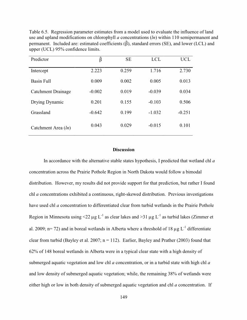
149

Table 6.5. Regression parameter estimates from a model used to evaluate the influence of land use and upland modifications on chlorophyll a concentrations (ln) within 110 semipermanent and permanent. Included are: estimated coefficients (β�), standard errors (SE), and lower (LCL) and upper (UCL) 95% confidence limits.

Predictor β� SE LCL UCL

Intercept 2.223 0.259 1.716 2.730

Basin Full 0.009 0.002 0.005 0.013

Catchment Drainage -0.002 0.019 -0.039 0.034

Drying Dynamic 0.201 0.155 -0.103 0.506

Grassland -0.642 0.199 -1.032 -0.251

Catchment Area (ln) 0.043 0.029 -0.015 0.101

Discussion

In accordance with the alternative stable states hypothesis, I predicted that wetland chl a

concentration across the Prairie Pothole Region in North Dakota would follow a bimodal

distribution. However, my results did not provide support for that prediction, but rather I found

chl a concentrations exhibited a continuous, right-skewed distribution. Previous investigations

have used chl a concentration to differentiated clear from turbid wetlands in the Prairie Pothole

Region in Minnesota using <22 µg L-1 as clear lakes and >31 µg L-1 as turbid lakes (Zimmer et

al. 2009; n= 72) and in boreal wetlands in Alberta where a threshold of 18 µg L-1 differentiate

clear from turbid (Bayley et al. 2007; n = 112). Earlier, Bayley and Prather (2003) found that

62% of 148 boreal wetlands in Alberta were in a typical clear state with a high density of

submerged aquatic vegetation and low chl a concentration, or in a turbid state with high chl a

and low density of submerged aquatic vegetation; while, the remaining 38% of wetlands were

either high or low in both density of submerged aquatic vegetation and chl a concentration. If

150

alternative states do exist, separation between the modes of each state should be more distinct in

a larger sample across landscapes within a region. Yet, I found more evidence to support a

continuous distribution.

There are alternative explanations as to why a continuous rather than bimodal distribution

better describes wetland chl a concentration evaluated across landscapes within the Prairie

Pothole Region. If state-change control points are driven by climate, chemical constituents,

nutrients, depth and wetland size (Scheffer and van Nes 2007), then heterogeneity among driving

factors increases the variation in those control points such that manifestation of each state can

vary from wetland to wetland. Accordingly, indicators of alternative states (e.g., chl a

concentrations) may vary among wetlands enough to appear continuously distributed. Individual

wetlands may indeed exhibit individual states, but among a large sample of wetlands across

landscapes the expected bimodal distribution of a state indicator for a single wetland could be

masked. Time-series analyses of chl a concentration within wetlands that are selected at random

across landscapes within the region might provide evidence to support this explanation.

However, if individual wetlands have different state-change control points that also lead to clear

versus turbid states defined at different chl a concentrations, the alternative stable state

hypothesis might not be useful for conservation planning at a landscape scale.

A second alternative explanation considers continuous changes in biological

communities and the potential for less abrupt transitions in trophic structure. This explanation is

not in line with the alternative stable states hypothesis, but rather proposes that trophic structure

in prairie wetlands is better explained within a continuum. Changes in dominant species of

algae, plants, and animals can occur gradually within wetland communities suggesting trophic

structure may change continuously at various rates (Scheffer et al. 1994; Van den Berg et al.

151

1999; Scheffer and van Nes 2007) rather than the abrupt or catastrophic changes illustrated in

some of the case-study wetlands. Certainly, catastrophic state changes as a result of reduced

nutrient inputs, biomanipulations, or winter-kill events have been documented by other

investigators (Scheffer et al. 1993; Hanson and Butler 1994a; Bayley et al. 2007; Hobbs et al.

2012). However, those cases were also the result of marked changes in stressors affecting those

wetlands. It is not clear if a catastrophic regime shift would have been observed if the change in

stressors were more gradual. More-abrupt changes in wetland trophic structure would be

expected to result from more-abrupt events such as biomanipulation which is essentially a

biological perturbation (Carpenter et al. 1985). Conversely, more physical perturbations like

increased sedimentation or changes in hydrology might actually produce more-gradual changes

in wetland community structure rather than the catastrophic changes predicted by the alternative

stable state hypothesis. Thus, a continuum of wetland communities might better describe

wetlands across these particular landscapes, rather than two distinctive, alternative states (van der

Valk 1981; Euliss et al. 2004). Further, the myriad physical and chemical factors that influence

biological communities in prairie wetlands (Weller and Spatcher 1965; Stewart and Kantrud

1972; van der Valk and Davis 1978; Euliss et al. 2004) have created more variety of wetland

conditions, trophic structures, and levels of biological productivity in prairie wetlands than can

be described by discrete states.

Distinguishing between biological, chemical, and physical perturbations might be useful

not only to determine rates of wetland community change, but potentially to understand potential

future wetland conditions or states (Euliss et al. 2004; Hanson et al. 2005). Shallow lakes have

been observed to alternate between states, returning to same state after biological state-changing

perturbations (Scheffer et al. 1993; Hobbs et al. 2012). However, if more physical disturbances

152

on adjacent uplands cause a change to the physical structure of the wetland system, a more-

permanent change could prevent a wetland from returning to a prior state. Two examples of

disturbances commonly imposed on wetlands in the Prairie Pothole Region are tillage of adjacent

uplands that increases sedimentation rates (Gleason and Euliss 1998) and drainage of smaller

wetlands to consolidate water into larger wetland basins (Anteau 2012; McCauley et al. In

Review; Chapter 2). Each of these perturbations could change the physical structure of the

wetland by altering wetland depth and consequently the wetland community.

Consolidation drainage can unbalance hydrologic dynamics (Chapter 2), resulting in

higher and more-stable water levels. Expanded wetland connectivity produced by higher water

levels can reduce basin isolation. Creation of more corridors for fish colonization will increase

the occurrence of sustained fish populations (Chapter 4), subsequently increasing turbidity in

fish-populated wetlands (Hanson et al. 2005). Fish occurrence in my study wetlands was not

independent of landscape modifications that altered wetland physical structure (Chapter 2–4);

therefore, I did not include “fish” among landscape variables in the model to explain chl a

concentrations. Colonization of fish into clear-water wetlands represents a biological

perturbation and changes in biological communities are often abrupt, reflecting catastrophic

changes in trophic structure (Carpenter et al. 1985; Scheffer 2001; Zimmer et al. 2003; Zimmer

et al. 2006). However, a model that uses landscape variables that are more-readily available than

are fish data (e.g., land use/land cover, hydrogeomorphology, and water levels) is likely more

useful for landscape- or regional-scale assessment of wetland condition and is more aligned with

practical conservation efforts.

Prairie wetland communities are typically regulated by fluctuation of water levels driven

by climate variability. These fluctuations likely maintain wetlands on the clearer side of the

153

continuum through elimination of fish and by improving growth conditions for submerged

aquatic vegetation. If disturbances like consolidation drainage reduce or eliminate the drawdown

portion of the cycle, then wetlands may become more turbid as these wetlands likely receive

more sediment and nutrients and are more likely to maintain a fish community. Alternatively,

water drawdowns in a turbid wetland could trigger a shift toward clearer-water through the

elimination of fish (Blindow et al. 1993; Bayley et al. 2007) and establishment of submerged

aquatic vegetation in the shallower water. Within a disturbed prairie landscape dominated by

turbid, water-stabilized wetlands, restoration of more-dynamic hydrology is likely a prerequisite

to the recovery of clear-water biological communities.

Grassland surrounding a wetland was an important predictor of chl a concentration in my

analysis. Relative to wetlands that are surrounded by grassland or that have little or no adjacent

cropland, wetlands surrounded by a high proportion of cropland likely receive significant

amounts of sediment delivered by wind and runoff water, and thus tend to be more turbid

(Gleason and Euliss 1998). Agricultural practices that have put more land into production have

increased the amount of exposed soil on the landscape (see Euliss et al. 2010). Sedimentation

has been identified as the leading pollutant in prairie wetlands, reducing the abundance of

submerged aquatic vegetation (USEPA 1995; Gleason and Euliss 1998). Furthermore, run-off

water and sediments can transport nutrients, salts and agricultural chemicals from fields to

wetlands, changing the chemical condition of the wetland (Neely and Baker 1989), potentially

increasing phytoplankton blooms, and increasing the probability of a wetland being turbid.

As a technical note, turbidity resulting from suspended sediments can affect in situ

measurements of chl a concentration. I found that controlling for turbidity measured by an

optical probe was essential to post-calibrate optical probe chlorophyll measurements to results

154

from laboratory assessment of chl a via fluorometry. Most large-particle constituents of turbidity

are filtered out of samples prior to laboratory fluorometry. Any optical sensor is likewise

affected by all sources of turbidity while making in situ measurements; therefore, turbidity likely

imposes variability in remotely-sensed chl a concentrations. I used a novel approach to account

for turbidity by incorporating near infrared (band 4) and short-wave infrared reflectance (bands 5

and 7) accounted for some of the variation associated with turbidity not due to chl a (Moore et al.

1999; Schalles 2006; Gilerson et al. 2010). Near infrared and short-wave infrared wavelengths

are mostly absorbed in clear water, but suspended solids in water will backscatter these

wavelengths increasing reflectance values in turbid water (Moore et al. 1999; Schalles 2006;

Gilerson et al. 2010). There is potential for further investigation to refine remote sensing

algorithms to better understand spectral signatures of wetland water types and vegetation

communities.

If alternative states do exist and can be defined in individual wetlands, understanding

regime-shift triggers and the resilience of biotic communities could allow managers to more

effectively manipulate wetland states where more detailed information is available on prior

perturbations and other drivers of biological communities. However, wetland chl a

concentrations resemble a continuous distribution across landscapes in the Prairie Pothole

Region of North Dakota. This, plus the fact that landscape variables better predict chl a

concentration as a continuous, not a binomial, distribution suggests that the alternative stables

states hypothesis might not be an appropriate framework for assessing processes relevant to

conservation of wetlands across the prairie landscapes. Accordingly, for the purposes of

improving conservation delivery and planning, I question the usefulness of characterizing

wetlands within an alternative stable state framework. Alternatively, evaluation of wetland

155

condition at a larger scale might best focus on simply evaluating patterns of anthropogenic

disturbances that correspond to degradation of wetland biological communities and their

ecological functions.

Literature Cited

American Public Health Association (APHA). 1998. Standard methods for the examination of

waste and wastewater. American Public Health Association, Washington, D.C., USA.







Anteau, M. J., and A. D. Afton. 2009. Wetland use and feeding by lesser scaup during spring










156

Bayley, S. E., I. F. Creed, G. Z. Sass, and A. S. Wong. 2007. Frequent regime shifts in trophic

states in shallow lakes on the Boreal Plain: alternative "unstable" states? Limnology and

Oceanography 52:2002–2012.

Bayley, S. E., and C. M. Prather. 2003. Do wetland lakes exhibit alternative stable states?

Submersed aquatic vegetation and chlorophyll in western boreal shallow lakes.

Limnology and Oceanography 48:2335–2345.

Blindow, I., G. Andersson, A. Hargeby, and S. Johansson. 1993. Long-term pattern of alternative

stable states in two shallow eutrophic lakes. Freshwater Biology 30:159–167.

Brivio, P. A., C. Giardino, and E. Zilioli. 2001. Determination of chlorophyll concentration

changes in Lake Garda using an image-based radiative transfer code for Landsat TM

images. International Journal of Remote Sensing 22:487–502.

Carlson, R. E. 1977. A trophic state index for lakes. Limnology and Oceanography 22:361–369.

Carpenter, S. R., N. F. Caraco, D. L. Correll, R. W. Howarth, A. N. Sharpley, and V. H. Smith.

1998. Nonpoint pollution of surface waters with phosphorus and nitrogen. Ecological

Applications 8:559–568.

Carpenter, S. R., J. F. Kitchell, and J. R. Hodgson. 1985. Cascading trophic interactions and lake

productivity. Bioscience 35:634–639.

Chander, G., B. L. Markham, and D. L. Helder. 2009. Summary of current radiometric

calibration coefficients for Landsat MSS, TM, ETM+, and EO-1 ALI sensors. Remote

Sensing of Environment 113:893-903.

Cheng, K. S., and T. C. Lei. 2001. Reservoir trophic state evaluation using Landsat TM Images.

Journal of the American Water Resources Association 37:1321–1334.

157

Cowardin, L. M., T. L. Shaffer, and P. M. Arnold. 1995. Evaluations of duck habitat and

estimation of duck population sizes with a remote-sensing-based system. U. S.

Department of the Interior, National Biological Service Biological Science Report 2,

26 p.

Dieter, C. D. 1990. The importance of emergent vegetation in reducing sediment resuspension in

wetlands. Journal of Freshwater Ecology 5:467–473.




458.

Euliss, N. H., Jr., L. M. Smith, S. Liu, M. Feng, D. M. Mushet, R. F. Auch, and T. R. Loveland.

2010. The need for simultaneous evaluation of ecosystem services and land use change,

7761–7763 p.

Folke, C., S. R. Carpenter, B. Walker, M. Scheffer, T. Elmqvist, L. Gunderson, and C. S.

Holling. 2004. Regime shifts, resilience, and biodiversity in ecosystem management.

Annual Review of Ecology, Evolution, and Systematics 35:557–581.

Gilerson, A. A., A. A. Gitelson, J. Zhou, D. Gurlin, W. Moses, I. Ioannou, and S. A. Ahmed.

2010. Algorithms for remote estimation of chlorophyll-a in coastal and inland waters

using red and near infrared bands. Optics Express 18:24109–24125.



158






Gunderson, L. H., and L. Pritchard, Jr. (eds). 2002. Resilience and the behavior of large-scale

systems. Island Press, Washington, D.C., USA.

Hanson, M. A., and M. G. Butler. 1994a. Responses of plankton, turbidity, and macrophytes to

biomanipulation in a shallow prairie lake. Canadian Journal of Fish and Aquatic Science

51:1180–1188.

Hanson, M. A., and M. G. Butler. 1994b. Responses to food web manipulation in a shallow

waterfowl lake. Hydrobiologia 279-280:457–466.




Hargeby, A., G. Andersson, I. Blindow, and S. Johansson. 1994. Trophic web structure in a

shallow eutrophic lake during a dominance shift from phytoplankton to submerged

macrophytes. Hydrobiologia 279/280:83–90.

Hobbs, W. O., J. M. R. Hobbs, T. LaFrançois, K. D. Zimmer, K. M. Theissen, M. B. Edlund, N.

Michelutti, M. G. Butler, M. A. Hanson, and T. J. Carlson. 2012. A 200-year perspective

on alternative stable state theory and lake management from a biomanipulated shallow

lake. Ecological Applications 22:1483–1496.

159

Holling, C. S. 1973. Resilience and stability of ecological systems. Annual Review of Ecology

and Systematics 4:1–23.

Irish, R. R., J. L. Barker, S. N. Goward, and T. Arvidson. 2006. Characterization of the Landsat-

7 ETM+ Automated Cloud-Cover Assessment (ACCA) Algorithm. Photogrammetric

Engineering and Remote Sensing 72:1179–1188.

James, W. F., and J. W. Barko. 1990. Macrophyte influences on the zonation of sediment

accretion and composition in a north-temperature reservoir. Archiv Fur Hydrobiologie

120:129–142.

May, R. M. 1977. Thresholds and breakpoints in ecosystems with a multiplicity of stable states.

Nature 269:471–477.



Moore, G. F., J. Aiken, and S. J. Lavender. 1999. The atmospheric correction of water colour and

the quantitative retrieval of suspended particulate matter in Case II waters: Application to

MERIS. International Journal of Remote Sensing 20:1713-1733.

National Aeronautics and Space Administration (NASA). 2014. MODIS Web: Data Products.

http://modis.gsfc.nasa.gov/data/dataprod/ - accessed: 09/15/2014.

National Agricultural Statistics Service (NASS). 2011. North Dakota Cropland Data Layer. U.S.

Department of Agriculture. http://nassgeodata.gmu.edu/CropScape/ - accessed:

9/24/2014.

Neely, R. K., and J. L. Baker. 1989. Nitrogen and phosphorus dynamics and the fate of

agricultural runoff. In A. G. van der Valk (ed) Northern prairie wetlands. Iowa State


160



Reynolds, R. E., D. R. Cohan, and M. A. Johnson. 1996. Using landscape information

approaches to increase duck recruitment in the Prairie Pothole Region. Transactions of

the North American Wildlife and Natural Resource Conference 61:86–93.

Sánchez-Carrillo, S., and M. Álvarez-Cobelas. 2001. Nutrient Dynamics and Eutrophication

Patterns in a Semi-Arid Wetland: The Effects of Fluctuating Hydrology. Water, Air, and

Soil Pollution 131:97-118.

Sass, G. Z., I. F. Creed, S. E. Bayley, and K. J. Devito. 2007. Understanding variation in trophic

status of lakes on the Boreal Plain: a 20 year retrospective using Landsat TM imagery.

Remote Sensing of Environment 109:127–141.

Schalles, J. F. 2006. Optical remote sensing techniques to estimate phytoplankton chlorophyll a

concentrations in coastal waterwith varying suspended matter and CDOM concentrations.

In L. L. Richardson, and E. F. LeDrew (eds) Remote Sensing of Aquatic Coastal

Ecosystem Processes: Science and Management Applications. Springer, Dordrecht, The

Netherlands.

Scheffer, M. 2001. Alternative attractors of shallow lakes. Scientific World Journal 1:254–263.

Scheffer, M., S. R. Carpenter, J. A. Foley, C. Folke, and B. Walker. 2001. Catastrophic shifts in

ecosystems. Nature 413:591–596.



161

Scheffer, M., S. Rinaldi, Y. A. Kuznetsov, and E. H. van Nes. 1997. Seasonal dynamics of

daphnia and algae explained as a periodically forced predator-prey system. Oikos

80:519–532.

Scheffer, M., M. van den Berg, A. Breukelaar, C. Breukers, H. Coops, R. Doef, and M.-L.

Meijer. 1994. Vegetated areas with clear water in turbid shallow lakes. Aquatic Botany

49:193–196.

Scheffer, M., and E. H. van Nes. 2007. Shallow lakes theory revisited: various alternative

regimes driven by climate, nutrients, depth and lake size. Hydrobiologia 584:455–466.

Stewart, R. E., and H. A. Kantrud. 1972. Vegetation of prairie potholes in North Dakota, in

relation to quality of water and other environmental factors. U. S. Department of the

Interior, Geological Survey, Washington, D.C., USA. Professional Paper 585-D.




Swanson, G. A., and H. K. Nelson. 1970. Potential influence of fish rearing programs on

waterfowl breeding habitat. In E. Schneberger (ed) Symposium on the management of

midwestern winterkill lakes. North Central Division of the American Fisheries Socitey,

Winnipeg, Manitoba, Canada, pp 65–71.

Timms, R. M., and B. Moss. 1984. Prevention of growth of potentially dense phytoplankton

populations by zooplankton grazing, in the presence of zooplanktivorous fish, in a

shallow wetland ecosystem. Limnology and Oceanography 29:472–486.

162




USA, pp 565–576.

Tyler, A. N., E. Svab, T. Preston, M. Présing, and W. A. Kovács. 2006. Remote sensing of the

water quality of shallow lakes: a mixture modelling approach to quantifying

phytoplankton in water characterized by high-suspended sediment. International Journal

of Remote Sensing 27:1521–1537.

U.S. Environmental Protection Agency (USEPA). 1995. National water quality inventory: 1994

report to Congress. Washington, D.C., USA.EPA Report 841-R-95-005.



U.S. Geological Survey. 2014. Earth Explorer. http://earthexplorer.usgs.gov/ - accessed:

09/15/2014.

Van den Berg, M., M. Scheffer, E. Van Nes, and H. Coops. 1999. Dynamics and stability of

Chara sp. and Potamogeton pectinatus in a shallow lake changing in eutrophication level.


van der Valk, A. G. 1981. Succession in wetlands: a Gleasonian approach. Ecology 62:688–696.

van der Valk, A. G., and C. B. Davis. 1978. The role of seed bands in the vegetation dynamics of

prairie glacial marshes. Ecology 59:322–335.

Vermote, E. F., D. Tanre, J. L. Deuze, M. Herman, and J. J. Morcette. 1997. Second Simulation

of the Satellite Signal in the Solar Spectrum, 6S: an overview. Geoscience and Remote

Sensing, IEEE Transactions on 35:675–686.

163

Weller, M. W., and C. S. Spatcher. 1965. Role of habitat in the distribution and abundance of

marsh birds. Iowa Agriculture and Home Economics Experiment Station, Special Report

43. Ames, Iowa, USA.

Zimmer, K. D., M. A. Hanson, and M. G. Butler. 2003. Relationships among nutrients,

phytoplankton, macrophytes, and fish in prairie wetlands. Canadian Journal of Fisheries


Zimmer, K. D., M. A. Hanson, B. R. Herwig, and M. L. Konsti. 2009. Thresholds and stability of

alternative regimes in shallow prairie-parkland lakes of central North America.

Ecosystems 12:843–852.

Zimmer, K. D., B. R. Herwig, and L. M. Laurich. 2006. Nutrient excretion by fish in wetland

ecosystems and its potential to support algal production. Limnology and Oceanography

51:197–207.

164

CHAPTER 7. GENERAL CONCLUSION

Waterbird conservation can benefit from evaluation of wetland habitat within watershed-

derived wetland complexes in the Prairie Pothole Region. These larger-than-wetland-scale

evaluations provide insight into processes that drive changes within remaining wetlands and

provide context to trends that may be important for understanding waterbird populations in the

region (Niemuth et al. 2009). Migrating and breeding waterbirds use complexes of wetlands

during each life stage (Skagen and Knopf 1994; Niemuth et al. 2006). Therefore, conservation

efforts need to be based on how wetland habitat availability is affected by landscape changes that

result from anthropogenic disturbances (Higgins et al. 2002), all in a temporal context of climate

variability and longer-term climate change (Johnson et al. 2010; Niemuth et al. 2010; Loesch et

al. 2012).

Identification of the implications that anthropogenic disturbances have on waterbird

habitat at landscape and regional scales can help prioritize effective conservation efforts. I found

that consolidation drainage has a progressive-chronic effect on the hydrology of more-permanent

wetlands by increasing the amount of surface water these wetlands receive, at a rate exceeding

their rate of water loss (Chapter 2). Thus, these wetlands increase in size until they fill their

topographic basin. Further, I speculated that wetlands occupying topographic basins that are

already full will spill additional drainage water to downstream watersheds, adding to regional

flood problems. In extensively drained catchments there are fewer small wetlands to provide

waterbird habitat, while productivity of remaining larger wetlands has been adversely affected

(Chapters 3–5). Drastic disturbances to natural wetland complexes, composed of wetlands

having various hydroperiods, have likely degraded overall landscape productivity of waterbird

food resources across wet–dry climate periods. This process has produced a landscape

165

increasingly composed of wetlands representing two extremes: drained former-wetland basins

and permanent lakes. This altered landscape is likely less able to provide necessary migration

and breeding habitat for waterbirds due to reduced productivity of essential plant and animal

forage (Afton and Anderson 2001; Anteau et al. 2011). In addition, structural changes to

wetlands may reduce the abundance of foraging habitat, especially for shorebirds (Niemuth et al.

2006; Anteau 2012).

Altered hydrology can change wetland communities and result in less biodiversity

dominated by less-desirable populations. Cattails or fish can become abundant in wetlands

where water levels have risen to fill more of their topographic basin, and where water-level

dynamics have been reduced (Chapters 3 and 4). Consolidation drainage can be indirectly linked

to increased abundances of cattails or of fish. Such changes ultimately lead to reduced wetland

quality, as defined by the ability to support diverse plant, invertebrate, and waterbird

communities.

Restoration of wetlands having various hydroperiods within watershed-derived wetland

complexes is likely the most effective approach to reversing the effects of consolidation drainage

(Anteau 2012). This strategy entails protection or restoration of temporary and seasonal

wetlands encompassed within the catchment of larger wetlands, such as semipermanent

wetlands. Conservation programs that purchase land, or gain easements, in areas without direct

control over wetland hydrology in the upper-portion of the watershed may be less effective than

efforts that directly protect or restore watershed-derived wetland complexes. However, degraded

catchments of protected wetlands may receive greater legal attention in the future if land use and

wetland drainage are strongly linked to declines in biological productivity and diversity.

166

Amphipod densities in wetlands across the region remain low compared to historical

accounts, despite hydrological conditions that were perceived to be prime for amphipod

production during the time of my observations (Anteau and Afton 2008; Chapter 5). Weak

evidence suggests that consolidation drainage has had a negative effect on amphipod densities in

wetlands. Nonetheless, 23%, 15%, and 6% of wetlands surveyed had >100 amphipods m-3

during 2004/05, 2011, and during both 2004/05 and 2011, respectively. This suggests that there

are still highly-productive wetlands in the region that provide forage for waterbird populations at

various phases within climate variability, and a sparse few wetlands appear to be consistently

productive. Further study of wetlands that are consistently highly productive might provide

significant insight into factors required for high invertebrate production in wetlands within the

region. Such additional research may improve our ability to identify and prioritize these types of

wetlands for cost-effective conservation at the landscape scale.

It may prove more useful for waterbird conservation to consider the frequency of highly

productive wetlands in the region than to focus on overall mean productivity, or to seek out

drivers of small changes in productivity within wetlands. Understanding local and landscape

factors that are related to either consistently productive wetlands, or wetlands in which

productivity is very dynamic, could help managers understand region-wide levels of productivity

through different phases of climate variability. To advance this goal, future research should

focus on identifying and intensely studying highly-productive wetlands, while making

comparisons to less-productive wetlands. This approach differs from previous regional-scale

investigations that typically select subject wetlands randomly, without prior knowledge of

system productivity. Such use of prior knowledge has the potential to improve study design,

statistical inference, and ultimately our understanding of wetland productivity.

167

There is potential for characteristics of highly-productive wetlands to be sensed remotely.

One such indicator of wetland productivity that can be remotely-sensed is chlorophyll a

concentration (Chapter 6). My data fail to support the alternative stable state hypothesis due to

lack of a bimodal distribution of chlorophyll a (Chapter 6). Nevertheless, chlorophyll a may be a

useful negative indicator of productivity within wetlands as it relates to available waterbird

forage, although perhaps within the framework of a continuum. Other indicators of wetland

productivity that could be remotely sensed might include vegetation structure, water quality (e.g.,

turbidity), wetland connectivity, and upland land cover/land use (Naugle et al. 2001). There are

several benefits to developing a model of highly-productive wetlands using remotely-sensed

data, including increased sample size and spatial distribution, and availability of historic data

(e.g., Landsat) to improve capability for time-series analyses. Time-series analyses using

remotely-sensed data have the greatest potential to better detect effects of landscape

modifications on wetland productivity in the context of climate variability, but this approach will

rely on predictions of productivity developed from less extensive studies.

Conservation programs focused on understanding how landscape modifications have

altered wetland productivity and that increase the frequency of highly-productive wetlands may

better manage long-term wetland quality for waterbirds across different phases of climate

variation. Within modified landscapes, recovering a balance between smaller, less-permanent

and larger, more-permanent wetlands, linked by through groundwater networks that fluctuate in

response to climate variability, will likely enhance waterbird habitat across wet–dry periods of

climate fluctuations. Identifying and protecting wetlands exhibiting consistently high levels of

productivity can be a more cost-effective model for conservation because these wetlands play a

vital role in supporting waterbird populations within the region. Better understanding of what

168

makes wetlands highly productive will lead to more effective conservation efforts. Such

knowledge will be useful in identifying landscapes where complexes of wetlands, with diverse

hydroperiods, can be restored potentially creating landscapes that maintain high productivity

throughout cycles of climate variability.

Literature Cited

Afton, A. D., and M. G. Anderson. 2001. Declining scaup populations: a retrospective analysis

of long-term population and harvest survey data. Journal of Wildlife Management

65:781–796.








Higgins, K. F., D. E. Naugle, and K. J. Forman. 2002. A case study of changing land use

practices in the Northern Great Plains, U.S.A.: an uncertain future for waterbird

conservation. Waterbirds 25:42–50.

Johnson, W. C., B. Werner, G. R. Guntenspergen, R. A. Voldseth, B. Millett, D. E. Naugle, M.

Tulbure, R. W. H. Carroll, J. Tracy, and C. Olawsky. 2010. Prairie wetland complexes as

landscape functional units in a changing climate. Bioscience 60:128–140.

169

Loesch, C. R., R. E. Reynolds, and L. T. Hansen. 2012. An assessment of re-directing breeding

waterfowl conservation relative to predictions of climate change. Journal of Fish and

Wildlife Management 3:1–22.

Naugle, D., R. Johnson, M. Estey, and K. Higgins. 2001. A landscape approach to conserving

wetland bird habitat in the prairie pothole region of eastern South Dakota. Wetlands

21:1–17.

Niemuth, N., M. Estey, R. Reynolds, C. Loesch, and W. Meeks. 2006. Use of wetlands by

spring-migrant shorebirds in agricultural landscapes of North Dakota’s Drift Prairie.


Niemuth, N. D., R. E. Reynolds, D. A. Granfors, R. R. Johnson, B. Wangler, and M. E. Estey.

2009. Landscape-level planning for conservation of wetland birds in the U.S. Prairie

Pothole Region. In J. J. Millspaugh, and F. R. Thompson, III (eds) Models for planning

wildlife conservation in large landscapes. Elsevier Academic Press, New York, NY,

USA, pp 553–560.

Niemuth, N. D., B. Wangler, and R. E. Reynolds. 2010. Spatial and temporal variation in wet

area of wetlands in the Prairie Pothole Region of North Dakota and South Dakota.

Wetlands 30:1053–1064.

Skagen, S. K., and F. L. Knopf. 1994. Migrating shorebirds and habitat dynamics at a prairie

wetland complex. Wilson Bulletin 106:91–105.

by mark thomas wiltermuth doctor of philosophy

Documents