by luis m. colon-perez
TRANSCRIPT

1
WEIGHTED NETWORKS AND THE TOPOLOGY OF BRAIN NETWORKS
By
LUIS M. COLON-PEREZ
A DISSERTATION PRESENTED TO THE GRADUATE SCHOOL OF THE UNIVERSITY OF FLORIDA IN PARTIAL FULFILLMENT
OF THE REQUIREMENTS FOR THE DEGREE OF DOCTOR OF PHILOSOPHY
UNIVERSITY OF FLORIDA
2013

2
© 2013 Luis M. Colon-Perez

3
To my wife and family

4
ACKNOWLEDGMENTS
I would like to thank Prof. Thomas H. Mareci for his support and guidance
throughout these past four years. His knowledge, input, and keen attention to detail
have been influential factors to my growth as a student and a researcher. I am grateful
for Prof. Mareci’s guidance in my MRI experiments and the numerous opportunities that
presented themselves while working in his lab, such as being able to make research
presentations in Canada and Australia. His mentorship has allowed me to grow not only
as a researcher, but also as a person. I would like to express my deepest gratitude to
Prof. Beverly Brechner. Her eagerness towards the research topic in this dissertation
and our insightful discussions were instrumental to my study of graph theory and
network theory. Her discussions had a great impact on the development of this work.
Last, but not least, I would like to thank Dr. Paul R. Carney, for the discussions, and the
research opportunities to work in his laboratory. I recognize that, even though these
research endeavors are not part of this dissertation, they did help me grow as a scientist
by showing me the broad spectrum of techniques and perspectives that can be used to
solve modern problems in the science of the brain.
I feel very fortunate to have been able to work in the Advanced Magnetic
Resonance Imaging and Spectroscopy (AMRIS) facility at the McKnight Brain Institute
at the University of Florida. The opportunity to work with world-class equipment and
staff at AMRIS is something to be really grateful for. I am especially thankful to Kelly
Jenkins, Barbara Beck, Dan Plant, and Huadong Zeng for multiple discussions and help
with setting experiments and solving hardware problems. Also, my deepest gratitude to
my lab mates: Mansi B. Parekh, Garret Astary, William Triplett, Christine Girard, Aditya
Kumar and Guita Banan. I will always remember the fun times in lab and hard work that

5
we all performed as a team. Also, I would like to show my deepest gratitude to the
undergraduates that helped me with the least fun part of this dissertation (node
segmentation): Caitlin Spindler, Shelby Goicochea, and Michelle Couret. I appreciate
their loyalty to stay with me and I hope you did learn something with me in lab. I would
also like to mention other undergraduate students that at some point have helped me
with my different investigations: R. Horesh, R. Klassen, E. Carmona and A. Boutzoukas.
Lastly, I would like to thank the Physics Department and the professors and staff for all
of their help in the past five years. Most importantly, my Physics dissertation committee
members: Prof. Mark Meisel, Prof. James Fry and Prof. Neil Sullivan.
Special contributions to this dissertation will be listed in this paragraph. Dr. M.
Parekh trained me in the diffusion weighted acquisitions and helped acquire data. Dr. G.
Astary was my MR tutor in lab and helped set up experiments. Mr. Triplett helped me
with the coding of the tractography software and made the first version of the software
used to perform the tractography work. Dr. E Montie, provided brain rats to study their
structural connectivity. Dr. C. Price provided the human data sets presented in this
dissertation. Miss S. Goicochea, Miss. C. Spindler and Miss. M. Couret, segmented the
rats nodes and assisted in the processing of the data.
I would like to extend a posthumous acknowledgement to my physics high school
teacher and mentor Miguel Baez. “Mister Baez” as everyone knew him, passed away in
March 2013 and, more than a teacher, he was an inspiration to many of his students,
including me. I will always remember the good chats and candid memories of my high
school years with him; may he rest in peace.

6
Finally, I would like to acknowledge the most important people in my life—my
family. My wife, Yarelis, who has supported me all these years and stuck with me even
with the long distance and sparse opportunities to see each other as often as we
wanted to. She was the source of inspiration to continue my studies and finish this PhD.
Also, I want thank my parents who raised me to become the person that is completing
this PhD work. I would like to thanks Carlos Poventud for being a great college and
even greater friend throughout my time in Puerto Rico and after I started my time here
in Florida. Their love, guidance, support, and encouragement helped me overcome all
adversities in these past years. Last, but not least, I want to thank my sister, Dialitza, for
all of her love and support in my life. She was a source of inspiration and
encouragement, as she recently graduated with her PhD in the past year, the first in our
family.

7
TABLE OF CONTENTS
page
ACKNOWLEDGMENTS .................................................................................................. 4
LIST OF TABLES .......................................................................................................... 10
LIST OF FIGURES ........................................................................................................ 11
LIST OF ABBREVIATIONS ........................................................................................... 14
ABSTRACT ................................................................................................................... 16
CHAPTER
1 INTRODUCTION .................................................................................................... 18
1.1. The Problem .................................................................................................... 19 1.2. Outline ............................................................................................................. 20
2 BACKGROUND ...................................................................................................... 22
2.1. Diffusion and MRI ............................................................................................ 22 2.1.1. Principles of Diffusion Displacement ...................................................... 22 2.1.2. Diffusion Weighted Imaging .................................................................... 24
2.2. Networks .......................................................................................................... 33 2.2.1. Graph Theory Metrics ............................................................................. 34 2.2.2. Random Networks .................................................................................. 38 2.2.3. Small World ............................................................................................ 41 2.2.4. Scale Free .............................................................................................. 42 2.2.5. Brain Networks ....................................................................................... 43
3 GENERAL METHODS ............................................................................................ 54
3.1. MRI Acquisition ................................................................................................ 54 3.1.1. Human Data ........................................................................................... 54 3.1.2. Animal Data ............................................................................................ 55
3.2. Post Processing ............................................................................................... 55 3.3. Tractography .................................................................................................... 56 3.4. Network Calculations ....................................................................................... 57
4 WEIGHTING BRAIN NETWORKS ......................................................................... 59
4.1. Opening Remarks ............................................................................................ 59 4.2. Methods ........................................................................................................... 60
4.2.1. Edge Weight ........................................................................................... 60 4.2.2. Edge Weight Derived from DWI ............................................................. 65

8
4.2.3. Simulations ............................................................................................. 67 4.2.4. Node Segmentation ................................................................................ 68
4.3. Results ............................................................................................................. 70 4.3.1. Simulations ............................................................................................. 71 4.3.2. Cingulum and Corpus Callosum Networks ............................................. 76 4.3.3. Limbic System Network .......................................................................... 79
4.4. Discussion ....................................................................................................... 82 4.5. Concluding Remarks ........................................................................................ 85
5 TOPOLOGY OF WEIGHTED BRAIN NETWORKS ................................................ 96
5.1. Opening Remarks ............................................................................................ 96 5.2. Methods ........................................................................................................... 97
5.2.1. Network Construction ............................................................................. 97 5.2.2. Null Hypothesis Graphs ........................................................................ 100
5.3. Network Metrics ............................................................................................. 101 5.3.1. Node Connectivity ................................................................................ 102 5.3.2. Average Weighted Path Length ............................................................ 102 5.3.3. Clustering Coefficient ........................................................................... 104 5.3.4. Small Worldness................................................................................... 105
5.4. Results ........................................................................................................... 107 5.5. Discussion ..................................................................................................... 116 5.6. Concluding Remarks ...................................................................................... 122
6 PATHOLOGICAL NETWORKS ............................................................................ 141
6.1. Opening Remarks .......................................................................................... 141 6.2. Methods ......................................................................................................... 142
6.2.1. Animals Treatment ............................................................................... 142 6.2.2. Networks .............................................................................................. 142
6.3. Results ........................................................................................................... 143 6.4. Discussion ..................................................................................................... 148 6.5. Concluding Remarks ...................................................................................... 153
7 FUNCTIONAL NETWORKS ................................................................................. 163
7.1. Opening Remarks .......................................................................................... 163 7.2. Theory ............................................................................................................ 164 7.3. Global Functional and Structural Networks .................................................... 166 7.4. Structural constraints to large DCMs ............................................................. 167
8 CONCLUSION AND FUTURE DIRECTIONS ....................................................... 170
8.1. Conclusions ................................................................................................... 170 8.2. Future Directions............................................................................................ 172

9
APPENDIX
A OPTOGENETICS AND FMRI ............................................................................... 178
B CONTINUOUS EDGE WEIGHT REPRESENTATION.......................................... 180
C COMPUTER CODES............................................................................................ 187
D AUTHOR’S PUBLICATIONS ................................................................................ 190
E GLOSSARY INDEX .............................................................................................. 191
LIST OF REFERENCES ............................................................................................. 192
BIOGRAPHICAL SKETCH .......................................................................................... 202

10
LIST OF TABLES
Table page 4-1 Edge weight values across the acquired ten data sets of 1 mm3 ........................ 95
4-2 Edge weight values across the acquired ten data sets of 8 mm3 ........................ 95
5-1 Average node degree values. ........................................................................... 139
5-2 Average node strength values. ......................................................................... 139
5-3 Binary path length and clustering coefficient metrics ........................................ 139
5-4 Weighted path length and clustering coefficient. .............................................. 139
5-5 Small worldness of weighted and binary networks. .......................................... 139
5-6 Human brain network nodes. ............................................................................ 140
6-1 Average degree ( ) values ............................................................................... 161
6-2 Average node strength ( ) values .................................................................... 161
6-3 Binary network metrics. .................................................................................... 161
6-4 Weighted network metrics. ............................................................................... 161
6-5 Small worldness ............................................................................................... 161
6-6 Rat brain network nodes.. ................................................................................. 162

11
LIST OF FIGURES
Figure page 2-1 Stejskal Tanner diffusion sequence .................................................................... 50
2-2 The effect of the b value on the estimation of the diffusion profile ...................... 50
2-3 The Königsberg map .......................................................................................... 51
2-4 Types of Graphs ................................................................................................. 51
2-5 The small world phenomenon............................................................................. 52
2-6 Scale free distributions in scale. ......................................................................... 52
2-7 Brain graph construction ..................................................................................... 53
3-1 Images of data used ........................................................................................... 58
3-2 Diagram of the tractography process .................................................................. 58
4-1 WM fiber connecting two nodes. ......................................................................... 87
4-2 A central node connected to four other nodes .................................................... 87
4-3 A sketch displaying the process used to obtain the set of seed points ............... 88
4-4 3D sketch of a system of 2 nodes connected by a fiber ..................................... 88
4-5 Slant fiber path connecting two nodes at different planes. ................................. 89
4-6 Segmentation of a 3-node and 2-edge system ................................................... 89
4-7 Human and rat brain networks............................................................................ 90
4-8 System of 2 nodes connected by a fiber at 45 degrees from the pixels .............. 91
4-9 Edge weight plots of arc and slants .................................................................... 91
4-10 Edge weight values for a slant in plane of single voxel nodes ............................ 92
4-11 Coefficient of variation (cv) plots as a function of σ levels. .................................. 92
4-12 Edge weight plots for the cingulum and corpus callosum tracts ......................... 93
4-13 Excised rat brain edge weight values in the TL network. .................................... 93
4-14 Excised rat brain node strength values in the TL network .................................. 93

12
4-15 Excised rat brain surface area values for the TL structures ................................ 94
4-16 Excised rat brain edge length values in the TL network. .................................... 94
5-1 Three-node network connected by two edges .................................................. 124
5-2 Eleven-node weighted network ......................................................................... 124
5-3 Graph density plot ............................................................................................ 125
5-4 Node degree measurements ............................................................................ 126
5-5 Node degree distribution .................................................................................. 127
5-6 Node strength values ........................................................................................ 128
5-7 Node strength distribution ................................................................................. 129
5-8 Representative binary and weighted adjacency matrices ................................. 130
5-9 Average binary path length distribution scale .................................................. 131
5-10 Average weighted path length distribution ........................................................ 132
5-11 Binary clustering coefficient distribution ............................................................ 133
5-12 Weighted clustering coefficient distribution. ...................................................... 134
5-13 Weighted clustering coefficient distribution ....................................................... 135
5-14 Anatomical location of human nodes ................................................................ 136
5-15 Streamlines connecting nodes………………………………………………............137
5-16 Differences in binary and weighted matrices. ................................................... 138
6-1 Degree values, results of rat networks ............................................................. 155
6-2 Degree distribution of rat brain networks .......................................................... 156
6-3 Node strength results of sparse networks. ....................................................... 157
6-4 Clustering coefficients distribution of sparse networks. .................................... 158
6-5 Anatomical location of rat nodes. ...................................................................... 159
6-6 Streamlines connecting nodes in the rat brain .................................................. 160
8-1 Resolution effects on town borders in Puerto Rico ........................................... 176

13
8-2 Validation of streamlines obtained with tractography with histology ................. 177
A-1 Optogenetic stimulation and activation captured with fMRI. ............................. 179
B-1 3D fiber sideways. ............................................................................................ 185
B-2 Sketch of one of the portions that make up the fiber. ....................................... 185
B-3 Sketch of the piece of the voxel that contributes to the edge. .......................... 185
B-4 Sketch of the isolated piece of the voxel contributing to the edge .................... 186

14
LIST OF ABBREVIATIONS
AD Average diffusivity
AM Amygdala
BOLD Blood oxygenated level dependent
CC Corpus callosum
DCM Dynamical Causal Model
DMN Default mode network
DTI Diffusion tensor imaging
DWI Diffusion weighted imaging
EC Entorhinal cortex
EPI Echo planar imaging
ER Erdös and Rényi
FA Fractional anisotropy
FACT Fiber assignment by continuous tracking
fMRI Functional magnetic resonance imaging
FOV field of view
GM Gray matter
HARDI High angular resolution diffusion imaging
HC Hippocampus
L Left side
MOW Mixture of Wisharts
MR Magnetic resonance
MRI Magnetic resonance imaging
NMR Nuclear magnetic resonance
PDF Probability displacement function

15
PR Puerto Rico
PTU Propylthiouracil
R Right side
SF Scale free
SNR Signal to noise ratio
SW Small world
TD Thyroid disruption
TE Echo time
TH Thalamus
TL Temporal lobe
TR Repetition time
WM White matter

16
Abstract of Dissertation Presented to the Graduate School of the University of Florida in Partial Fulfillment of the Requirements for the Degree of Doctor of Philosophy
WEIGHTED NETWORKS AND THE TOPOLOGY OF BRAIN NETWORKS
By
Luis M. Colon-Perez
August 2013 Chair: Thomas H. Mareci, Ph.D. Major: Physics
The brain is a network characterized by high clustering and short distances
between nodes. The topological framework used to quantify these properties assumes
that connections are equivalent and that networks are sparse, which is not an accurate
assumption for the brain. Consequently, there is a need to generate metrics that
resemble the physical substrate of brain networks, which would lead to properly
weighted networks. This dissertation describes a novel edge-weight, which is a
dimensionless, scale-invariant measure of node-to-node strength connectivity in brain
networks derived from magnetic resonance imaging (MRI). Edge-weight simulations
were performed on multiple fiber structures, displaying higher accuracy with high seed
points per voxel and when random errors were kept below a standard deviation of less
than 0.03. This implies that high seed density and signal to noise ratio is required to
employ the edge-weight.
The framework used to estimate the topological features of networks is
generalized to study weighted brain networks. The framework allows the study of
topological properties in dense weighted networks, which otherwise would not be

17
possible. Human and rat diffusion weighted images (DWI) were acquired in a 3T and
17.6T magnet respectively. The DWI data was used to construct the brain networks and
the generalized framework was able to demonstrate the small world property in
situations where the binary framework failed. In dense binary networks (when the
number of edges is 50% or more than all possible node-pairs combinations), the brain
displayed organization similar to a random network while dense weighted networks
displayed increased clustering suggesting a small world organization. This suggests a
new way of looking at structural brain networks derived from MRI as a dense mesh of
weighted connections, arranged in an efficient and robust manner.
Finally as a perturbation model, thyroid disrupted rat brain networks were
analyzed and revealed that the brain exhibits small world properties even after
perturbations. This implies that the network is organized to preserve effective global
communication and specialized processes. The weighted networks and framework
presented in this dissertation provides a more realistic model to describe brain networks
and eliminates the sparseness requirement to determine network organization.

18
CHAPTER 1 INTRODUCTION
Although the brain’s ability to wonder and inquire has permitted us to understand
many aspects about our bodies, the environment, and the universe, much is left to
understand about the brain itself. The brain is the substrate where all knowledge
originates. Neuroscience has guided most of our understanding of the brain; however,
physics can finally provide its own contribution with the development of novel
techniques and modeling to further comprehend the complexity of our brains.
The idea of looking at the structure of complex systems as a network became a
useful tool as the limitations of working with isolated components of the system became
understood (i.e. reductionism is not enough) (Barabási, 2011; Glickstein, 2006). The
study of networks has yielded a wealth of knowledge regarding the topological
organization of large-scale systems (Craddock et al., 2013). The topological traits of real
complex networks have been widely studied by mostly assuming binary interactions
between the components of the network. However, the representation of these systems
as either connected or not connected (i.e. simple graphs) is not sufficient. The
binarization of interactions yields a topological framework that allows us to study
complex networks and estimate the organizational features of real world networks.
However, the framework itself is not flawless; it comes with ambiguities in the definition
of connections and assumes that networks are sparse.
The connections in the binary framework, by definition, are present or absent,
assuming all connections as equivalent in their strength. This binary framework has
been used because it was the natural progression of the field and simplification of
network interactions as equivalent provided helpful information regarding the structure

19
of real systems. However, it is unrealistic to assume equivalency in the connection
strength between components of most real systems. Also, the sparseness condition is
associated with the fact that the strongest connections are most confidently measured.
Devising methods to quantify the strength of a connection requires a system-by-system
analysis. Once acceptable measurements become available, network properties can be
estimated from more complicated graphs (i.e. weighted, multigraphs).
1.1. The Problem
While representing real world systems as networks, one must consider the
heterogeneity of connections in the real world. This is a useful and necessary concept
to represent the real system as a network. The structure of real networks should not be
assumed to have equivalent connections, nor should these connections be considered
sparse. Therefore, it is essential to develop novel methods that can define edges with
their associated strength within the network (i.e. weighting the network). Also, to
characterize the real structure of networks, the binary framework must be generalized to
account for the new degree of freedom that is associated with the heterogeneity of
edges in the weighted network.
The ability to quantify the brain’s complex structure permits us to infer the basic
principles of brain organization and formation. The structural organization of networks
can be studied at different levels or scales, which are representative of the interaction
between components. The brain has three levels: microscale, mesoscale and
macroscale (explained in Chapter 2). To discover universal principles of network
organization, an adequate framework must be created to study networks at all levels.
Many networks, although different in nature, share basic principles; therefore, being

20
able to understand how networks form and how they are structured for a given system
might provide the necessary insight to understand all networks. A proper framework
might elucidate new principles of the real structure of networks that would not have
been possible with a binary approach.
Generalized frameworks permit the estimation of structural organization allowing
researchers to gain insight into the features of real world networks from models that
closely resemble the real substrate. Such an approach would take us a step closer to
accurately describing the brain as a complex network, without losing the important
information obtained from binary approaches, and providing new information to
understand the brain’s structural organization in greater detail. Also, the generalization
of the framework would be a necessary advancement to deal with networks in a more
realistic manner, as long as an appropriate characterization of the physical strength of
connectivity is accomplished.
1.2. Outline
In this dissertation, developments made in complex network analysis are
presented. In Chapter 2, the background of diffusion is reviewed and briefly discussed
as it relates to the different structures of the brain. Also, a brief discussion on graph
theory developments is revisited. This is followed in Chapter 3, with an introduction of
the MR methods used in Chapters 4 through 6. In Chapter 4 a new definition of an edge
weight, based on a previous edge weight by Hagmann et. al. (Hagmann et al., 2008),
derived from DWI and tractography is presented. Chapter 5 introduces a generalized
framework to analyze weighted networks, which is a new approach to estimate
topological characteristics in weighted networks. The combination of Chapters 4 and 5

21
present a novel method to weigh brain networks derived from MRI and tractography in
relation to the physical substrate. In Chapter 6, effects of network perturbations are
addressed in brain networks that give rise to structural reorganizations. The
perturbations are due to white matter loss resulting from thyroid hormone disruption in
rat brains. In Chapter 7 a roadmap to merge structural networks with functional models
is shown. Finally, Chapter 8 summarizes the findings and gives an overview of the
current state of the field and possible future directions.

22
CHAPTER 2 BACKGROUND
2.1. Diffusion and MRI
Diffusion is the tendency of particles to move at random via collisions within a
medium. It gives us the ability to understand the properties of materials and study
environmental structures (e.g. porous media). Currently, the study of diffusion allows
scientists to better understand the brain’s vasculature (Assaf et al., 2008),
compositional changes in the presence of disease (Jellison et al., 2004), and overall
structural organization (Hagmann et al., 2007; Iturria-Medina et al., 2007). The random
motion of water molecules helps describe tissue boundaries and arrangement, which
ultimately allow the estimation of the complex structure and network of the brain (Assaf
and Basser, 2005; Basser et al., 1994; Conturo et al., 1999; Ozarslan et al., 2006).
2.1.1. Principles of Diffusion Displacement
Diffusion allows particle mixing without bulk motion (Crank, 1980), a process
commonly related to mass transport. Employing Fick’s laws of diffusion, this process
can be expressed mathematically, in an isotropic medium, where the media structure
permits substances to have the same diffusive properties at any location (Phillips et al.,
2008). Fick’s first law of diffusion relates diffusive flux to a gradient in concentration as
CDJ ∇⋅−= . (2-1)
In Equation 2-1, J represents the particle flux, C is the particle concentration, and D is
the diffusion coefficient. The diffusion coefficient is a property of the medium, depending
on the particles undergoing diffusion and the environmental structures. Fick’s first law

23
describes the flux, J, in a system with an inhomogeneous spatial concentration of at
least two substances. The direction of the flux will be opposite to the gradient of the
concentration (i.e., particles in the area of higher concentration will migrate to areas of
less concentration) until equilibrium is reached and a homogenous distribution is
obtained. Fick’s second law of diffusion (Equation 2-2) is obtained by employing two
conditions: (i) the conservation of particles and (ii) continuity such that the change in
concentration over time is due to particle flux in the system as
( )CDtC
∇⋅∇=∂∂
. (2-2)
At this point, from Equation 2-2, it appears that once a gradient of concentration
vanishes, the flux will vanish as well and diffusion would stop. However, the particle’s
random motion, driven by thermal energy, continues even at equilibrium. Since diffusion
is constrained by the structural geometry of the environment, diffusion with nuclear
magnetic resonance (NMR) provides a unique foundation to obtain information about
the internal structure of a system. Therefore the diffusional properties of water
molecules can be exploited in the study of brain structure using magnetic resonance
imaging. In 1827, Robert Brown, a Scottish botanist, observed pollen grains and
inorganic particles moving when suspended in water (Brown, 1828). Although in the
system there is no net flux or gradient of concentration, Brown observed molecules
moving. He called these active molecules organic and inorganic bodies. In 1905, Albert
Einstein, examining the existence of atoms, showed that particles of microscopic size
would move when suspended in water (Einstein, 1905). Einstein’s work proved that
Brown’s active molecules were the manifestation of molecule collisions (driven by the
thermal energy) with the liquid molecules in the system. Einstein’s 1905 publication on

24
the studies of small particles in liquid would consolidate Brown’s observations with the
predictions obtained by molecular kinetic theory of heat. Einstein goes on to state that
“bodies of microscopically-visible size suspended in a liquid will perform movements of
such magnitude that they can easily be observed in a microscope, on account of the
molecular motions of heat”. Then he states that the molecular motions he discussed
could be identical to Brownian motion, and over time this statement has been accepted
as the reason for the observed motion of Brown’s particles. Also Einstein’s description
of the diffusion of small spheres in suspension led to Equation 2-2 hence unifying the
Fickian and Brownian descriptions of particle diffusion. These diffusion descriptions
helped characterize diffusion behavior in NMR experiments (Carr and Purcell, 1954;
Torrey, 1953) as will be shown in the next section. This ultimately led to diffusion
weighted MRI (DWI).
2.1.2. Diffusion Weighted Imaging
In 1956, H. Torrey modified the phenomenological NMR’s Bloch equations
(Equation 2-3 and known as the Bloch-Torrey equation) to explain the change in
magnetization due to the thermal motion of water molecules (Torrey, 1956). The
modification consists of the addition of a diffusion term analogous to the right hand side
of Equation 2-2. In Equation 2-2 diffusion is due to changes in concentration while in
Equation 2-3 it is due to the transfer of magnetization by diffusion.
MDMMT
MMT
BMγdtMd T
xyz ∇⋅⋅∇++−−+×=
)(1)(121
(2-3)
where, M stands for the magnetization of water molecules in an applied magnetic field, γ

25
represents the gyromagnetic ratio of the particles, B is the applied magnetic field, T1
longitudinal relaxation time, T2 is the transverse relaxation time and D is the diffusion
coefficient. The first term on the right contains the effects of the magnetic field on the
total magnetization, M; this causes the precession of spins around the main magnetic
field B. The spins will precess at a frequency characteristic of its nucleus leading to the
rate of precession known as the Larmor frequency (ω, Equation 2-4) (Haacke et al.,
1999). The Larmor frequency is determined by
Bγω = (2-4) is the angular velocity of particles rotating in a magnetic field. The Bloch-Torrey
equation represents the macroscopic change in time of the magnetization in a system
where the particles that make up the macroscopic magnetization also undergo diffusion.
The second term is the yields the time dependence of the longitudinal magnetization
(around main magnetic field) as it returns to equilibrium and the third term yield the time
dependence of the transverse magnetization. From now on relaxation effects are
disregarded, since the experiments in this dissertation will consist of attenuation
measurements that estimate an effective scalar diffusion coefficient that is averaged
over the echo time. Later it will be shown that this measurement is only due to diffusion
contributions and independent of relaxation times.
In 1965, Stejskal and Tanner developed modern diffusion MRI measurements
(Stejskal and Tanner, 1965), to capture the diffusion effect in NMR by applying short
duration gradient pulses, as Figure 2-1 shows. In a spin echo experiment, as the one
shown in Figure 2-1, the time to repeat the entire encoding scheme (time between 90°
pulses) is known as TR and the time between the 90° pulse and the time it takes to

26
obtain a signal is TE. The Stejskal and Tanner method precisely defines the time period
in which the gradients are applied, and the time between gradients, so that diffusion can
be quantified. The first diffusion pulse gradient produces a phase shift that depends on
the position of each particle along the direction of the pulse gradient. In the absence of
diffusion, the second gradient would undo the phase shift due to the first gradient and
the loss of coherence would be negligible. However, as particles diffuse, the refocusing
of the second pulse becomes incomplete and causes an attenuation or signal loss. With
this method, the first pulse applies a spatially dependent phase change, such that when
the second pulse is applied, it forms a net phase change in the form of
( )1212 xxqφφ −−=− (2-5) where q = γδg, δ is the diffusion pulse length, g is the gradient strength, and x1 and x2
are the particles’ positions at the time of the first and second pulse, respectively
(Bernstein et al., 2004). In the Stejskal and Tanner approach the application of the
pulses are made “short” enough so that molecular displacements are negligible small
during δ compared to the diffusion time, Δ (i.e. δ<<Δ). The signal, which is given by the
magnetic moments of all spins, is attenuated due to the incoherence in the orientations
of the individual magnetic moments due to their thermal motion. This leads to a phase
change because of the change in their positions. Solving Equation 2-3 assuming T1~∞
and a spin echo sequence as shown in Figure 2-1, yields Equation 2-6, which shows
the signal obtained during a spin echo DWI experiment.
( )2
2
/3Δ
)( TTEδgγδD
o eeSqS −
−−
= (2-6) where So is the rate without diffusion weighting. Given the time scales (long TR’s and

27
long TE’s) in diffusion weighted experiments, the contrast will come predominantly from
T2 and diffusion.
Diffusion experiments seek to study the effect of the gradient pulses on the echo
amplitude. Hence, the diffusion signal is more conveniently written by the echo signal,
E(q) (Equation 2-7). The echo signal is a quantity obtained by taking the ratio of the
attenuated signal and the signal without any diffusion weighting, E(q)= S(q)/ So.
Therefore, the attenuation (Equation 2-7) is due to only diffusion effects and removes
relaxation effects by dividing by So. Equation 2-7 employs a normalized spin density
such that when no diffusion weighting is applied E(q)=1.
∫ ∫ −−⋅= 12)(
21112)Δ,,()()( dxdxexxPxρqE xxqi
(2-7)
where ρ(x1) is the normalized spin density at the time of the first pulse and P( x1, x2, Δ)
is the diffusion propagator (Green’s function) (Callaghan, 1991). The propagator is a
function that represents the likelihood that a particle initially at position x1 ends up in
position x2 after a time Δ, which is the time between gradients. The rate of signal loss,
or attenuation, for a given gradient strength is greatest when the gradients are applied
along a direction of small or no obstruction, and it is least for a gradient perpendicular to
a barrier or a restriction. In the Stejskal & Tanner approach, the solution to Equation 2-7
can be written as (Basser, 2002)
bDeqE −=)( . (2-8)
where
−=
3Δ)( 2 δgγδb . (2-9)
In Equation 2-6, the term in brackets will be referred throughout this text as the b value

28
(Equation 2-9), which is a quantity of the influence of the gradients in the diffusion-
weighted image. Important to note is the fact that the diffusion coefficient in Equation 2-
8 is written in terms of a scalar apparent diffusion coefficient. This means that the
measured E(q) will be dependent on the applied direction of the diffusion gradient or b
value direction. The bD term in the echo signal is the inner product of those quantities.
Therefore, every measurement along a different diffusion gradient direction will yield a
different diffusion coefficient which describes the influence of the diffusion gradient
direction in relation with the microstructure orientation within the voxel. For example the
echo signal will be minimal (attenuation will be maximal) when the gradient is parallel to
a WM fiber and maximal (attenuation will be minimal) when WM structures are
perpendicular to the gradient direction.
In practice, during the pulse gradient sequence, the molecules displace in the
order of 100 Å to 100 µm over time scales of a few milliseconds to a few seconds
(Callaghan, 1991). The dimensional scale of the pulse gradient scheme corresponds to
an organizational domain that includes features of macromolecular solutions, porous
solids, and biological tissue. The orientation dependence of the measured diffusion
coefficient will enable the modeling of the microstructure in a more complex manner.
Therefore, using pulse gradient NMR, one can probe the internal structure of the brain.
With the obtained MR signal, multiple models of diffusion can characterize the
properties of diffusion within the tissue: diffusion tensor, a distribution of second rank
tensors, and a model of constricted and hindered diffusion (Assaf and Basser, 2005;
Basser et al., 1994; Jian et al., 2007b).

29
The first model of diffusion to be introduced was the diffusion tensor ( D ) or,
diffusion tensor imaging (DTI) which corresponds to a second order tensor that
estimates the average diffusion coefficient in a voxel1 of the MR image (Basser et al.,
1994).
=
zzyzxz
zyyyxy
zxyxxx
ddddddddd
D
,,,
,,,
,,,ˆ (2-10)
where dij corresponds to the components of the diffusion tensor. In order to estimate the
diffusion tensor, a minimum of seven measurements are needed: a low or no diffusion
weighting and six diffusion weighted images. The six images includes: three along the
orthogonal directions (e.g. {x,y,z}) and three for crossed terms (e.g. {xy, xz, yz}) in
Equation 2-10. The tensor has antipodal symmetry, (i.e., it will always be symmetric)
and therefore only needs six component measurements, instead of all nine. This model
assumes Gaussian diffusion profiles in each voxel to estimate the diffusion tensor. This
has been a very successful model in obtaining diffusional properties of regions with
strong and coherent WM structures like the spinal cord, corpus callosum and cingulum;
however, it fails in regions where multiple fiber orientations appear. The Gaussian
diffusion condition limits the model to regions of single fiber orientation or free diffusive
water (e.g. cerebral spinal fluid). Diagonalization of the diffusion tensor as
uλυD ⋅=⋅ˆ , (2-11)
allows for the estimation of the average diffusivity (AD=⟨𝐷⟩,
1 Voxel is the 3D analog to a pixel

30
3
3
1∑== i
iλD , (2-12)
which is a measure of the self-translating diffusion within each voxel. Finally the
fractional anisotropy (FA, Equation 2-13) (Basser and Jones, 2002) can also be
obtained by
( ) ( ) ( )23
22
21
321
23
λλλDλDλDλ
FA++
−−−−−= (2-13)
which is a measure of the deviation from isotropic diffusion in each voxel. These
measures allow the discrimination of GM regions (high AD and low FA) from WM (high
FA and low AD). The recognition of anatomical structures is limited by the ability to find
contrast between tissue types, hence FA and AD greatly aids in tissue contrast hence
improving the ability to segment brain regions. In Equations 2-11 to 2-13, u represents
the eigenvectors or the principal diffusion directions and the λ’s are the eigenvalues.
In the brain, water molecules are present in the intra and extra axonal
compartments, which lead to restricted and hindered diffusion, respectively. The intra
axonal or restricted diffusion is observed over length scales of less than 2 µm.
Technological advantages of stronger magnetic fields allow the probing of the diffusion
within this compartment by applying stronger diffusion weightings. This prompted the
development of a new methods with improved acquisition techniques to model diffusion
like Diffusion Spectrum Imaging (DSI) (Wedeen et al., 2005), High Angular Resolution
Diffusion Imaging (HARDI) (Tuch et al., 1999) and the Composite Hindered and
Restricted Model of Diffusion (CHARMED) (Assaf and Basser, 2005; Assaf et al., 2004).
The DSI model uses the diffusion propagator of Equation 2-7 and samples diffusion on

31
a Cartesian space (i.e. q space, Equation 2-5). Employing the propagator’s Fourier
relation between the obtain signal and the mean particle displacement DSI is able to
characterize diffusion. HARDI, on the other hand, measures apparent diffusion
coefficient along many directions. From HARDI acquisitions more sophisticated models
of diffusion can be applied to represent diffusion profiles on each voxel. A method is
called the Method of Wisharts (MOW), Equation 2-14 (Jian et al., 2007a; Jian et al.,
2007b) to avoid DTI’s uncertainty in regions with multiple fibers a method. MOW is
based on HARDI acquisitions and was consists of fitting a distribution of tensors on
each voxel given by
( )∑=
−=n
i
gDgb iT
en
qE1
ˆˆ1)( . (2-14)
This model assumes that a mixture of diffusion tensors can characterize the
diffusion in each MR voxel. In this model, multiple tensors in the MOW distribution will
yield the fiber orientation. This allows resolving the regions of multiple directions within a
voxel. In this model, increased noise levels makes it more challenging to estimate the
fiber orientation when there are more than three fiber orientations. In this model, there is
no distinction between the different compartmental contributions to the signal
attenuation from the different biological compartments. The last model to be described
here, CHARMED, assumes two water compartments (one hindered and another
restricted) on each voxel where the diffusion attenuation arises. DSI and CHARMED
requires the acquisition of multiple shells of diffusion weightings where each additional
shell is the amplification or increase of the diffusion weighting, b value, and the number
of gradient directions. Although this model is the most physically feasible, it requires a

32
high number of diffusion weightings, thus making the acquisition protocol highly time
consuming. Since MOW is able to reconstruct multiple fiber orientations in each voxel
and is more applicable in many practical situations (i.e. clinical) will be employed in this
investigation.
To apply any of these methods, optimized acquisition protocols are needed to
better estimate diffusion profiles to reduce noise and angular uncertainty. The
optimization of b values (Equation 2-9) will better estimate the diffusion properties in
different regions of the brain. Since white matter fiber tracts, which are bundles of
neuronal axons, hinder diffusion of water molecules in neural tissue, the measured DWI
will depend on the structures and their orientation along the gradient directions. It has
been shown that at low b values the angular dependence of the signal in a plane
containing 2 distinct fiber directions is small, and diffusion direction estimation is very
noise sensitive, as seen in Figure 2-2 (Tournier et al., 2004). Contrastingly, high b
values enhance angular dependence; however the signal attenuation can get large
enough so the noise begins to dominate. Therefore, intermediate b values provide
better results because strong angular dependence is introduced without attenuating the
signal to noise level. A good compromise between b value and signal to noise ratio
(SNR) is needed to achieve high angular acquisition to accurately estimate diffusion and
obtain reliable fiber tracking. High angular resolution will aid in regions where fibrous
tracts cross (i.e., fibers travel one on top of another in a MR voxel, or kiss, i.e. the fibers
get close but do not cross). As the b value is optimized, the gradient direction scheme
can also be adjusted.

33
Performing additional measurements along a high number of gradient directions,
reduces bias introduced by measuring signal attenuation along a limited number
directions and diffusion estimation profile is improved in highly anisotropic areas (Jones
et al., 1999). Gradient schemes can also be optimized to improve the acquisition
scheme by increasing the number of diffusion directions. This work will employ an
optimized scheme of gradient directions described by Jones et al (Jones and Leemans,
2011). To optimize the diffusion directions of the gradient vectors, Jones applies the
criterion that these directions should be uniformly distributed in 3D space, analogous to
electrostatic repulsion that uniformly distributes charged particles onto a sphere. Jones’
model considers a line parallel to each gradient vector that passes through the center of
a sphere and a unit electrical charge is placed at both points where the line intersects
the sphere. A total of 64 charges (this number can be varied as desired) are allowed to
move, according to Coulomb’s repulsion law, until the sum of the electrical repulsion of
all charges is minimized. Thus, 64 direction gradient vectors are obtained to distribute
the diffusion weightings for imaging. These two approaches, b value and gradient
direction schemes, will be employed to improve the angular quality of the diffusion
weighted images.
2.2. Networks
Graph theory is the framework for the mathematical treatment of networks. A
network refers to a real system that is represented by a mathematical graph. The origin
of graph theory is attributed to Leonhard Euler and his study of the Königsberg riddle.
The city of Königsberg, presently called Kaliningrad in Russia, was separated by the
Pregel River and contained two islands, as shown in Figure 2-3, which were connected

34
by a set of seven bridges. In 1736, Euler solved the path riddle of the bridges (Newman,
2010), which inquired about the possibility of finding a path through the city crossing
each of the bridges only once. The residents of Königsberg tried without success to find
such path. In order to solve the riddle, Euler abstracted the city as a set of nodes (the
land masses) and edges (bridges), which became the Königsberg graph, Fig 2-4b.
Euler noticed that if a walker were to traverse only once through the bridges, they would
have to enter and leave each node an even number of times except at the beginning
and the end of the path (i.e., first and last nodes). All nodes in Figure 2-4b have an odd
number of connections. Euler’s abstraction of the network as a graph, proved the
impossibility of finding the riddle’s path. This proof was the first work using graphs to
represent a real network (Albert and Barabási, 2002) and provides the basis for dealing
with real systems as connected units forming a network.
2.2.1. Graph Theory Metrics
Graph theory represents a network as a graph, G = [N, E], where N is the set of n
nodes and E is the set of m edges in the network (Rosen, 2003). The basic components
of a graph are the nodes (e.g., people, web sites, or specific parts of the brain) and the
edges (i.e., the connections or interactions between different nodes) (Butts, 2009).
Mathematically, there are two basic descriptions that can be used to represent a graph:
the incidence matrix, M, and the adjacency matrix, A. The incidence matrix, M = [mij], for
a simple and undirected graph (described in the next paragraph) is a rectangular n x m
matrix for a set of nodes, N = {n1, n2, n3,…, nn} and edges, E = {e1, e2, e3,…, em} with a
specified ordering of the nodes and edges. The element of the incidence matrix mij is
non-zero when ej is incident on ni and zero otherwise. The adjacency matrix is a square,

35
symmetric matrix, n x n, for simple and undirected graphs, where n is the number of
nodes in the network, and A is written as
=
nnn
n
aa
aaA
1
111
(2-15)
where
=.,0
,otherwise
n to n connecting edge anis there ifzero nona ji
ij (2-16)
The adjacency matrix represents specific connections between nodes, where the
aij element of this matrix is non-zero if the node ni is connected to nj by an edge, and
zero otherwise. The non-zero elements of A will be determined depending on the type
of graph being employed to describe the network. There are four main types of
networks described by graph theory: simple, multigraph, directed, and weighted. The
nature of the connections in the network will determine the type of graph to be
employed.
The most basic type is the simple graph. In this graph, the edges are
directionless (i.e., an edge from ni to nj is equivalent to the edge from nj to ni as shown
in Fig 2-4a). The elements of the matrix are one when an edge connects the nodes and
zero otherwise. In addition, self-connections or multiple edges connecting the same two
nodes are not allowed. Therefore, adjacency matrices of simple graphs are always
symmetric and their trace is 0. Simple graphs will be referred through this text as binary,
since the connectivity is characterized by the presence or absence of edges.

36
A second type of network is the multigraph, which allows the presence of self-
connections or loops, also multiple edges connecting the same two nodes (e.g., the
Königsberg riddle of Figure 2-3 and 2-4b). However, similar to simple graphs, the edges
of multigraphs are directionless. The adjacency matrices of multigraphs are always
symmetric and their trace is not necessarily zero. The element aij of multigraphs will
reflect the number of edges connecting ni to nj and the trace of A will be twice the
number of loops in the graph. By definition, a loop connecting ni to itself is assigned the
number two. In simple graphs, an edge connecting node ni to node nj provides two
elements of the adjacency matrix; aij = 1 and aji = 1. Therefore, each end of every edge
contributes twice to the adjacency matrix. Similarly, by definition a loop is counted twice.
A loop will have two ends connecting to the same node yielding a value of two for aii.
Another type of graph is a directed graph. In these graphs, as the name suggests,
edges describe a direction of flow. In simple and multigraphs, information can flow in
either direction along the edges. In directed graphs, the adjacency matrix is defined as
follows: aij = 1 if the edge is directed from i to j, while aij = 0 otherwise.
Up to this point, all the discussed networks (simple, multigraph, and directed) are
described mathematically by integers (i.e., the number of edges connecting any two
nodes). However, for the last network type, weighted networks do not need integers
describing the connectivity. In these networks, the elements of A reflect strength of
connectivity between any connected pair of nodes in a graph. For the sake of simplicity
in this introductory chapter the network metrics described will be for simple graphs (i.e.
binary networks).

37
The adjacency matrix allows the determination of network parameters such as: 1)
the node degree, which is the number of edges that connect to a specific node; 2) the
path length, shortest path along the edges of the network to connect ni to nj; and 3) the
clustering coefficient, which measures the tendency of nodes to cluster. The simplest
measure that describes a network is the degree, k, (Equation 2-17) of each node. It is
calculated as
∑=
=N
jiji ank
1)( (2-17)
where aij is the ijth element of the adjacency matrix. The degree distribution provides a
simple topological representation of the number of links that any given node holds and
provides insights on the connectivity arrangement in the network.
Another commonly used metric is average path length, which measures the
average number of steps that connects any node to all others. Average path length
relates how efficiently information is transferred globally within the network. The path
length is calculated as given by
1)( 1
−=∑=
N
snl
N
jij
i (2-18)
where sij represents the minimal number of steps it takes to travel along the edges of
the graph from node i to node j, and N is the number of nodes in the network. In the
brain, the path length is associated with the efficiency of the overall structure of the
network (Bullmore and Sporns, 2009). Ideally, if only a few steps are needed to travel
from any node to any other node, information will most likely be transferred very
efficiently within the network.

38
The clustering coefficient, ci, measures the level of connectivity of the neighbors
of node ni or local connectivity around the neighborhood of ni. It measures the ratio of
the overall number of triangles that any node forms with its neighbors to the total
number of possible connections. The clustering coefficient of node ni considers the
neighbors nj and nk. If nj and nk are connected, then they form a triangle centered around
ni which contributes to the clustering coefficient value of node ni. The normalization [ki
(ki-1)/2] in the clustering coefficient is the total number of pair connections among the
neighbors if node i. The binary form of ci is specified by
∑=−
=−
=N
kjkijkij
iiii
jkBi aaa
kkkkE
c1,
, )1(1
)1(2
(2-19)
where Ei,k is the number of edges connecting the neighbors of node i. In the brain, the
clustering coefficient has been associated with specialized processing (e.g. sensory
input analysis, like visual, auditory, and so forth) (Bullmore and Sporns, 2009). Nearby
nodes work together to achieve complex tasks; therefore, high node clustering of the
neighbor nodes allows the efficient communication and ultimately complex task
processing.
2.2.2. Random Networks
In 1959, Paul Erdös and Alfred Rényi introduced the first model to generate
random graphs (also known as ER graphs)(Erdös and Rényi, 1959) This model was the
first one used to address questions relevant to network analysis using probabilistic
methods as the number of edges is increased. As an example, the ER model described
the probability of obtaining a giant component in a graph (a giant component is a

39
maximal set of nodes that are connected by a finite number of steps). Essentially this is
the point at which the graph starts to appear connected and the isolated nodes or
clusters of nodes are greatly reduced.
The construction of a random graph, G(n,p), starts with n nodes, and all edges
have equal probability p of connecting any pair of nodes, independently of the others
(Boccaletti et al., 2006). This is the first model using graphs to study the properties of
large-scale networks. The properties of these graphs are usually studied as an
ensemble of random graphs constructed with a specified number of nodes, and a
probability, p, that any pair of nodes is connected. In this model, the probability to find
any graph, G, is given by
mn
m ppGP−
−= 2)1()( . (2-20)
where m is the number of edges in the graph. Equation 2-20 leads to the probability of
having a graph with m edges from the ensemble of the form of Equation 2-21 (i.e. a
standard binomial distribution) (Newman, 2010), given by
mn
m ppm
nGP
m
nmP
−
−
=
= 2)1(2)(2)( . (2-21)
From Equation 2-21, and some simple arithmetic the mean number of edges can be
found as
pn
mmPm
n
m
== ∑
= 2)(
2
0, (2-22)
which is the total possible number of node-pairs times the probability, p, that they are
connected (Equation 2-22) (Newman, 2010). Since the edges are randomly distributed

40
throughout the entire graph, the mean degree can be estimated using Equation 2-22,
which leads to a mean degree of 2m/n for the entire graph. In this case, most of the
nodes in the graph will have an average degree
pnpn
nmP
nmmkPk
n
m
n
m)1(
22)(2)(
2
0
2
0−=
=== ∑∑
=
=, (2-23)
which is equal to the total number of nodes in the network minus one (itself, since it is a
simple graph) times the probability, p, that any pair of nodes are connected.
These mathematical descriptions of networks do not satisfy the observed
organizational and communication properties of real networks (Barabási and Albert,
1999; Milgram, 1967). This is not a surprise since it is not realistic to assume that all
connections are equivalent and equally probable. Erdös and Rényi recognized the
failure of their hypothesis in their work, “On the evolution of random graphs” (Erdös and
Rényi, 1960) where they refer to the evolution of certain communication networks, like
electric network systems;
“If one aims at describing such real situation, one should replace the
hypothesis of equiprobability of all connections by some more realistic
hypothesis”
Erdös and Rényi were more concerned with the mathematical treatment of
networks rather than fully understanding the intricacies and details of real network
formation. However, their work served as the mathematical basis of network studies
until new mathematical models of networks were introduced almost 40 years later.

41
2.2.3. Small World
At some point in our lives, we all have said “what a small world!” whenever we
find out that the person we have just met is a family member of our best friend, that a
co-worker we have worked with for some time is actually best friends with our cousin,
and many more familiar situations that we can all relate to. This phenomenon is actually
referred to in science by the same expression—the “small world” phenomenon (Watts,
2003). Stanley Milgram first introduced this phenomenon to science in 1967 with his
letters on the mail experiment (Milgram, 1967). Milgram asked a group of individuals to
send a letter from Kansas to Massachusetts, with the restriction that each sender had to
send it to an acquaintance who was most likely to know the final recipient. At the time,
the only network model was the random model introduced by Erdos and Renyi, which
led to the expectation that letters would travel at random through the 200 million
inhabitants of the United States until it would reach the final recipient. However, to
Milgram’s surprise, the letters that reached the final recipient arrived with an average
number of five intermediaries. This result contradicted common knowledge at the time
about network organization. It would take another 30 years to find a suitable
mathematical network model to describe this phenomenon.
In 1998, Watts and Strogatz introduced the small world model to explain
observations of the properties of real networks (Watts and Strogatz, 1998). The model
attempted to replicate the observed organizational feature of high clustering, which is
associated to the structure of regular graphs, and also short path lengths, associated
with random graphs. Studies of real-world networks (e.g., the world wide web (www))
repeatedly revealed a mixture of properties from random and regular graphs. The small
world model displayed the observed property that some real-world networks are neither

42
regular (i.e. all nodes have same degree) nor random. Figure 2-5 illustrates these
differences. Regular networks emphasize lattice-like arrangement of the nodes, as in
the atoms of a lattice from solid-state physics, where the connections between
components of the lattice are well known and ordered. Regular graphs exhibit the
properties of high clustering coefficients and long path lengths, while random graphs do
not emphasize any arrangement among nodes. Random graphs, in contrast to regular
graphs, exhibit low clustering coefficients and small path lengths. The small world
networks display some arrangement, yielding a high clustering coefficient as seen in
regular graphs. Additionally, it establishes some arbitrary connections that allow the
network to display small path lengths as seen in random graphs.
2.2.4. Scale Free
In 1999, studies of large-scale networks, such as the www, revealed another
feature that the previous two models had failed to show. Barabási found a long tail in
the degree distribution of real networks, such that a small, but significant, number of
nodes contained a very high number of connections, referred to as hubs. He coined the
term “scale free” (Barabási, 2009) to name these networks, due to the inability to obtain
a meaningful mean degree from these networks. In Figure 2-6, a power law is shown, a
long tail can be seen, where the black line represents an exponential decay associated
with small world networks. The exponential decay description shows that the graph is
unlikely to have degrees much different from the mean. However, the power law that
characterizes scale free networks implies that degrees much different from the average
are still likely to occur. In Figure 2-6 the probability of having nodes with degree 10

43
increases by 10 and 100 times for power laws with λ equal to three and two,
respectively.
A fundamental difference between the scale free model and both the ER and
small world models is the fact that the scale free model relies on growth and preferential
attachment (Barabási, 2003). The fact that the number of www websites or nodes is
dynamic allows one to think in a growth situation with a “first come, first serve”
assignment of the connections within the web. Originally, the graph is very small and, as
time progresses; one might think that the older nodes might lead to a hub-like status
over time. However, growth alone is insufficient to account for the extremely large hubs
in the www and other real world networks. Preferential attachment is introduced to bias
newcomers in the network to preferentially attach to high degree nodes. These two
conditions of preferential attachment and growth were sufficient to replicate the degree
distributions observed in the www and many other systems.
2.2.5. Brain Networks
Similar to the dispute on the nature of light, where Huygens argued for a wave
description of light while Newton claimed that particles were the basic nature of light,
neuroscience had a controversy regarding the nature of the basic organization in the
brain. Ramon y Cajal argued for a neuron doctrine while Golgi argued for a reticulum or
a network description (Glickstein, 2006). Ramon y Cajal’s interpretations and simplicity
of experiments led to the widespread consensus regarding the neuron being the basic
component of the brain. However, after a century of many advances, science has come
to the conclusion that to fully understand the brain, the neuron is insufficient (Sotelo,
2011). The interactions of neurons within brain regions are key to understand our

44
cognition and complex functioning. A rebirth of the network notion as a basic structure
to describe the brain appeared to provide a new way to further understand the
intricacies of brain structure and function. Although the neuron has been commonly
accepted as the basic component of brain structure, a network description would not
defy this consensus because the basic object of study in the brain network would be the
neuron and its interactions among other neurons (Sporns, 2011).
A growing interest to provide new ways to study the brain (Crick and Jones,
1993) has constantly been producing novel methods to determine brain structure in vivo
(Bassett and Bullmore, 2006; Bullmore and Sporns, 2009; Guye et al., 2010; Hagmann
et al., 2010a; Honey et al., 2010; Lo et al., 2011; Rubinov and Sporns, 2010; Sporns et
al., 2005; van den Heuvel and Sporns, 2011). High angular resolution diffusion imaging,
HARDI, (Tuch et al., 2002) and graph theory provide an ideal foundation to study the
brain structure non-invasively. The contrast due to local tissue structure (i.e. gray matter
(GM) and white matter (WM)) is greatly enhanced in HARDI measurements (Basser and
Jones, 2002). HARDI, along with advanced models that quantify diffusion parameters
(Jian et al., 2007b; Ozarslan et al., 2006; Tuch, 2004), allow the reconstruction of WM
fibers using tractography, even in complex tissue regions where fibers kiss or cross.
Using tractography techniques and graph theory, brain networks can be recreated by
representing anatomical regions as nodes, and the WM fibers connecting these nodes
as edges.
The characterization of brain graph topology can be made by estimating node
degree, path length, and clustering coefficient and determining connectivity patterns in
the brain (i.e. verifying which areas of the brain are connected). Network models can be

45
used not only to advance the knowledge regarding our brains, but also to provide
information about the formation and organizational features of networks in general. The
brain is a complicated network composed of billions of neurons connected by axons and
dendrites. In the last two decades, developments in the treatment of real systems has
led to complex networks science (Newman, 2010). Although complex networks may be
very different in their microscopic details, most share a similar macroscopic organization
(Barabási, 2009). Brain structural systems have features of complex networks, such as
small path length and high clustering, at the cellular level, as well as in the level of
anatomical regions. Therefore, complex network analysis provides an ideal framework
to study the brain structure.
To understand brain structure, the brain needs to be examined at three size
scales: microstructure, mesostructure and macrostructure (Sporns et al., 2005). The
microstructure deals with single neurons and synapses. The mesostructure refers to
anatomical cells grouping and their projections. Finally, the macrostructure deals with
brain regions and their connecting pathways. At the current technological state of MRI
and tractography, only the macroscopic structure is a reasonable starting point for the
study brain networks. Neuron size can vary in diameter from 4 to 100 μm, but most
often varies from 10 to 25 μm. Assuming a standard MRI voxel size of of 1 mm3 and a
neuron radius of 20 μm, a single voxel might contain 70,000 to 80,000 neurons.
Common DWI image resolution is 8mm3; so in this case each voxel contains close to
600,000 to 650,000 neurons. For these reasons the discussion will be limited to the
macrostructure of the brain.

46
Within the macroscale, there are two possible networks to study: local and
global. Local networks refer to anatomical structures connected to form a network with
only a few nodes that are closely related to specialized functions (Catani and Ffytche,
2005; Colon-Perez et al., 2012). Global networks will be associated with the study of
cortical structures or large-scale structures of the brain. Given the resolution and lack of
neuronal specificity of MRI, the nodes will be related to known macroscopic anatomical
regions. This allows us to assume that functional regions will be constrained within
anatomical regions. Several reports segregate random nodes in the cortex; however,
this assumes a functional homogeneity within the cortex that is not realistic (Bassett et
al., 2011b; Cammoun et al., 2011; Hagmann et al., 2007). Functional regions might
overlap with random node placement and connections might be confounded with a lack
of care for the integrity of functional domains in the node definition. A way to possibly
overcome the ambiguity of defining nodes might be through the use of functional MRI
(fMRI).
In 1990, Ogawa et. al. described changes in MR signal due to changes in blood
oxygenation levels (Ogawa et al., 1990). This blood oxygenated level dependent
(BOLD) signal is the basis of fMRI. The BOLD signal results from increased blood flow,
blood volume, and oxygen consumption. These hemodynamic changes (or BOLD
signal) are preceded by neuronal activation. As neurons activate, they consume
oxygen, energy, glucose, glutamate and lactate (Magistretti and Pellerin, 1999;
Magistretti et al., 1999). Glutamate has been shown to be necessary to explain the link
between oxygen and energy consumption with neural activity (Magistretti et al., 1999).
However, oxygen is the main contributor to the BOLD signal so neuronal consumption

47
of glutamate, glucose and lactate will not be addressed for this discussion, since these
do not affect significantly the measured response in the brain using fMRI. Neuronal
activation is associated with increases in the blood flow and blood volume locally in the
active region. The blood flow increases the amount of deoxygenated blood (which is a
paramagnetic molecule) inducing a field change which leads to a local reduction of the
field homogeneity (due to the susceptibility difference between deoxygenated blood and
the surrounding tissue). The susceptibility difference creates a frequency shift (Δω =
ɣΔB) hence reducing the T2* locally (1/T2
*=1/T2 + ɣΔB). This reduction in T2* is measured
with MRI as a decrease in the signal strength in the location of active neurons. Usually
neuronal activation is made possible by some sort of stimulation or function (e.g. hand
movements, visual stimulation and so on). Hence, using fMRI one can deduce which
regions are associated with the particular function used in the experiment. Up to this
point it has been discussed that functional and structural brain networks can be further
understood by the use of MRI, specifically fMRI and DWI respectively.
Functional analysis of brain networks can be made with optogenetics which
allows one to deliberately select specific regions (instead of stimulating by function,
which yields a response in the entire brain) to determine the functional connectivity from
the targeted region with the rest of the brain. Optogenetics is a method that allows one
to study the functional connectivity of the brain in such a way that neurons are made
sensitive to light via viral transduction of a light sensitive ion channel (channel rhodopsin
or ChR2) from algae (Lee et al., 2010). In optogenetics the CamKII promoter is used to
specifically target excitatory neurons. As light is shined onto the transduced neurons,
the ion channel opens up causing the neuron to become activated. This method allows

48
the activation of specific regions in the brain that can be used to study their functional
connectivity (Appendix A for details of preliminary work).
With graph theory, the brain can be described as a network. Current network-
based studies focus on determining the topological traits of the brain. Brain networks
are currently studied in vivo with magnetic resonance imaging (MRI) to create structural
connectivity maps via diffusional properties of tissue and tractography. Graph theory
provides the most commonly employed framework to study connectivity in the brain.
Evidence of scale free and small world organization has been found in the brain with the
use of functional MRI (fMRI) (Eguiluz et al., 2005; Tomasi and Volkow, 2011; van den
Heuvel et al., 2008). On the contrary, the use of diffusion MRI, tractography, and
structural studies suggests only a small world organization for brain networks (Bassett
et al., 2011b; Hagmann et al., 2007; He et al., 2009). A four part process is used to
develop such a model, as shown in Figure 2-7; (i) define networks nodes, (ii) define
network edges, (iii) estimate a connectivity matrix and (iv) calculate network parameters
(Bullmore and Sporns, 2009).
Brain network analysis will benefit by devising methods to obtain global network
characteristics in more realistic models. Weighted networks aids in the development of
this endeavor since weights in the graph can be associated with the physical substrate
of the edge. The main network metrics used to calculate networks properties are: 1)
degree, 2) path length, and 3) clustering coefficients. In this dissertation an edge weight
is presented to quantify the structural connectivity between any two nodes in the brain.
Then a generalization of network metrics is used to measure network properties in
weighted brain networks derived from tractography. Finally an assessment of the

49
weighted framework is made by comparing thyroid disrupted rat brains with normal
brains. The discussion in this dissertation from this point on will be limited to simple
graphs and the networks they represent (as a way to compare with more traditional
results obtained in literature) and weighted graphs and the networks they represent.
Directed graphs will not be considered since brain networks obtained from MRI do not
reflect any directionality in the connectivity pattern of the edges.

50
Figure 2-1. Stejskal Tanner diffusion sequence: Shown is a spin echo sequence with two short duration diffusion gradients applied after each radio frequency pulse. The radio frequency pulses will give rise to the measured magnetization. The time δ, is the duration of the diffusion gradient, and time Δ is the time between gradients. The diffusion gradient duration is set to be “short” so that the diffusion undergone by the spins in δ is negligible compared to Δ.
Figure 2-2. The effect of the b value on the estimation of the diffusion profile: Top: the noiseless signal attenuation profile in the plane of the fibers for a system consisting of two fiber populations crossing at 90°. Bottom: the corresponding fiber orientation distribution function for SNR = 30. The mean fiber ODF is depicted by the opaque surface, and the mean fiber standard deviation by the transparent surface. Left to right: b value increasing from 1000 to 5000 s/mm2 in increments of 1000 s/mm2. Image from Tournier, et. Al. (Tournier et al., 2004). Reproduced with approval from Elsevier.

51
Figure 2-3. The Königsberg map: The islands are represented by the green and yellow
dots and the large land masses are represented by the blue and red dots. Bridges are shown in turquoise. (Picture modified from engraving by Joachim Bering (Public domain, 1613))
Figure 2-4. Types of Graphs: A) Displays a simple graph. B) Multipgraph representing the city of Königsberg (Nodes’ color corresponds to the nodes in Figure 2-3). C) Sketch of a directed graph, top node is a source and bottom node is a sink. D) Weighted graph, thicker edge represents largest edge weight value.

52
Figure 2-5. The small world phenomenon: Graphs arranged; regular, small world and random graphs. (Figure form Watts et al. (Watts and Strogatz, 1998)). Reproduced with approval from Nature Publishing Group.
Figure 2-6. Scale free distributions in log-linear scale: Plot of the power law behavior in observed degree distributions from scale free networks. The exponential decay is associated with real, small world networks.
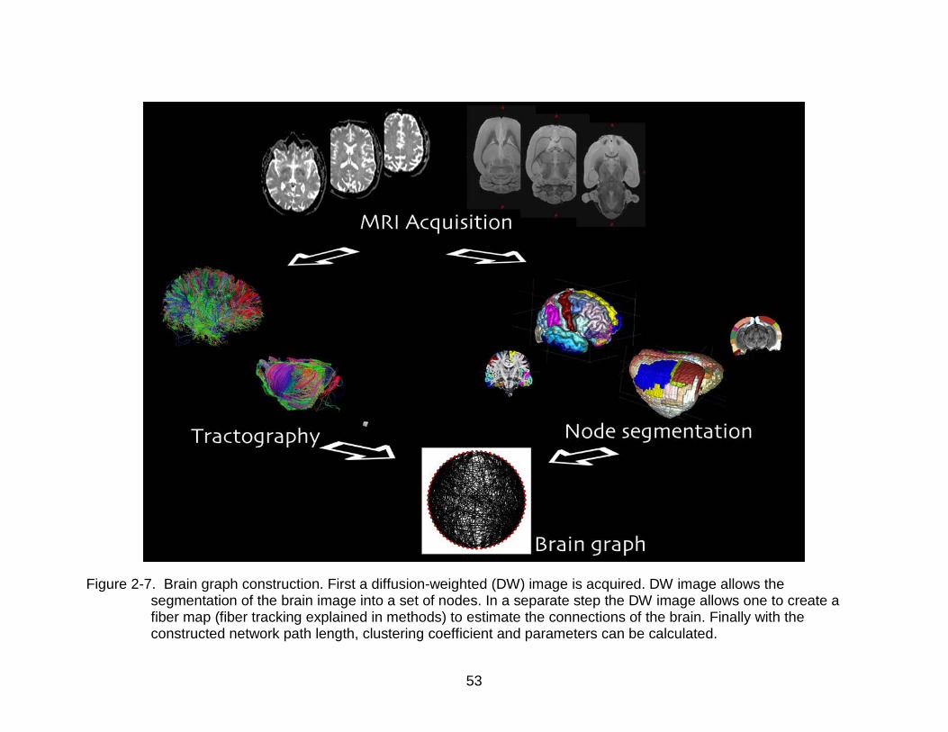
53
Figure 2-7. Brain graph construction. First a diffusion-weighted (DW) image is acquired. DW image allows the segmentation of the brain image into a set of nodes. In a separate step the DW image allows one to create a fiber map (fiber tracking explained in methods) to estimate the connections of the brain. Finally with the constructed network path length, clustering coefficient and parameters can be calculated.

54
CHAPTER 3 GENERAL METHODS
This chapter reviews the common techniques employed in the next three
chapters of this dissertation. Firstly, the human and rat acquisition schemes are
explained. Then the software and post processing techniques are reviewed. Lastly the
tractography is reviewed and the software for the network calculation is presented.
3.1. MRI Acquisition
3.1.1. Human Data
The University of Florida Institutional Review Board approved all human studies.
One healthy subject was scanned ten times throughout the course of one month, which
provided a controlled set of ten brain networks to determine the network properties
across different MR acquisitions. The subject was scanned in a 3T Siemens Verio
system in the Shands Hospital of the University of Florida. HARDI data was obtained
with a spin echo preparation and an EPI (Poustchi-Amin et al., 2001) readout and the
following set of parameters: TR/TE = 17300/81 ms, 2 scans without diffusion weighting,
6 diffusion weightings with b-values (Equation 2-9) of 100 s/mm2 and 64 diffusion
weightings with b-values of 1000 s/mm2 (Figure 3-1). The diffusion gradients were
distributed following a scheme of electrostatic repulsion (Jones et al., 1999). The
diffusion-weighted images covered the entire brain with an isotropic resolution of 2.0
mm, field of view (FOV) of 256 mm x 256 mm and 73 slices, which interpolated to 1.0
mm isotropic with tri-cubic interpolation. In addition, a high-resolution T1 structural scan
of the entire brain was acquired with TR/TE = 2500/3.77 ms, resolution 1mm isotropic,
FOV of 256 mm x 256 mm and 176 slices.

55
3.1.2. Animal Data
Four excised 90-day-old normal rat brains were scanned at the Advanced
Magnetic Resonance Imaging and Spectroscopy (AMRIS) facility of the McKnight Brain
Institute at the University of Florida with repeats of two brains for a total of six data sets.
HARDI data was obtained using a 17.6 T Bruker Avance system (Bruker Corp, Billerica,
MA) with the following set of parameters: 7 diffusion weightings with b values of 100
s/mm2 and 64 diffusion weightings with b values of 2225 s/mm2. The diffusion gradients
were distributed following the scheme of electrostatic repulsion. An image resolution of
190 x 190 x 190 μm3 was acquired; therefore this data set will be referred to throughout
this text as the 190 μm data set. Two new data sets were created for each of the six
data sets by interpolating the original image to 95 x 95 x 95 μm3, referred to as the 95
μm data set, and degrading it to 380 x 380 x 380 μm3, referred to as the 380 μm data
set, by using only half of the original k-space (Fourier transform of the MR image)
information to reconstruct the image. Representative images of these data sets are
shown in Figure 3-1.
3.2. Post Processing
The diffusion weighted scans were corrected for motion distortion using FSL’s
eddy_correct algorithm (Jenkinson et al., 2012). With the motion corrected data, FA and
AD maps were created using in-house software using the Interactive Data Language
(IDL; Exelis Visual Information Systems, Boulder, CO). The probability displacement
function (PDF) was calculated on each voxel using a mixture of Wishart (MOW)
distribution of positive definite matrices (Jian et al., 2007b) implemented with an in-
house C based software. Using the root mean displacement in three dimension

56
(x2 = 6Dt , where t = Δ - δ/3), the PDF was estimated in each voxel for an average water
displacement of 13 μm (human data) and 6 μm (rat data), then the maximum
displacement probability within tissue in each voxel is identified and associated as the
local fiber orientation. The nodes were created by visual inspection using ITKSNAP
(Yushkevich et al., 2006) to delineate the desired structures on the FA and AD maps.
For human data, the node segmentation was performed on a single data set (the first
one acquired) at the 1 mm x 1 mm x 1 mm resolution data set, then registered to the
other nine data sets using FSL’s FLIRT and ApplyXFM (Jenkinson et al., 2012). Then
these nodes were then registered onto the 2 mm x 2 mm x 2 mm data set from its
correspondent 1 mm x 1 mm x 1 mm data set by applying an identity transformation
using ApplyXFM. The node segmentation for the rat data was performed using the 95
μm resolution FA map. These nodes were then registered onto the 190 and 380 μm
date sets by applying an identity transformation using ApplyXFM. Details of node
placement will be addressed in each subsequent section.
3.3. Tractography
The fibrous structures of the brain are estimated from diffusion-weighted data by
creating fiber maps using tractography. These are calculated by deterministic streamline
tractography in the whole brain employing the MOW-derived fiber orientations.
Tractography was performed following a modified version of the fiber assignment by
continuous tracking (FACT) algorithm (Mori et al., 1999), in which the direction with the
least angular deviation along the incoming fiber path was selected to be continued at
each iteration of the tractography process. In many brain regions WM fibers cross or
kiss, so DTI cannot model the diffusional characteristics in these regions by just a single

57
Gaussian diffusion tensor per MR voxel, as explained in Chapter 2. Therefore MOW is
used to estimate the multiple fiber orientations in each MR voxel, yielding a more
accurate description of fiber directions. Fiber maps were calculated using an in-house C
based software. To avoid the ambiguity of random placement of seed points, these
were placed uniformly throughout the MR voxels making up the brain. Tractography is
performed by seeding each MR voxel in the brain with any number P of evenly-spaced
seed points. From each seed point, one streamline is launched bi-directionally for each
estimated displacement probability maximum contained in that voxel with the modified
FACT algorithm. Each streamline front is propagated by stepping half of the MR voxel
width in the direction that is most in line with the streamline's present direction of travel
(i.e. tractography generated smooth and no sharp turns) as shown in Figure 3-2.
Tractography parameters were: 125 seeds per voxel, a fiber step size of 0.5 of the voxel
size, and no step-to-step track deviations greater than 50o and stopping criteria for
voxels with low anisotropy values (FA < 0.05). If the estimated track exceeds this
threshold, the streamline is stopped.
3.4. Network Calculations
All network metrics were calculated in R (http://cran.us.r-project.org/), with the aid
of the network package (http://cran.r-project.org/web/packages/network/index.html).
The network package is a set of tools to create and modify network and relational data
within the R interface. All the networks metrics described in Section 2 were calculated
with in-house written software. All network metrics were calculated with the equations
presented in this manuscript (Chapter 2 for binary metrics and Chapter 5 for weighted
metrics). A copy of the most complicated of the codes can be found in Appendix C.

58
Figure 3-1. Images of data used. Human data shown in left column and rat data to the right. A) T1 weighted image at 1mm isotropic resolution. B) DW image at the acquired resolution of 2mm isotropic. C) Interpolated DW to 1 mm isotropic resolution. D) Acquired DWI at 190μm isotropic resolution. E) Interpolated DWI to 95μm isotropic resolution. F) Degraded DWI to 380μm isotropic resolution
Figure 3-2. Diagram of the tractography process. The first image on the left shows the seed points that starts each fiber. Each point is evenly spaced in the entire brain. The middle figure displays the calculated fiber orientations. This image shows 2 fiber orientations in each voxel. The image in the right shows the fiber propagation across the entire image. Each seed point contributes with two fibers because there are two fiber orientations in each voxel, but once a streamline is started it will follow the direction most in line with its path.

59
CHAPTER 4 WEIGHTING BRAIN NETWORKS
4.1. Opening Remarks
Graph theory studies applied to brain networks have gathered a great deal of
interest in large part due to the desire to analyze the large-scale cortical structure of the
brain (Bassett et al., 2011a; Cheng et al., 2012a; Costa Lda et al., 2007; Gong et al.,
2009; Hagmann et al., 2008; Hagmann et al., 2007; Romero-Garcia et al., 2012; Sporns
et al., 2007). In addition to cortical analysis, graph theory has been applied to
understand the relation between brain network structure and brain development
(Hagmann et al., 2010b) or pathological states like: epilepsy (Ponten et al., 2009),
schizophrenia (van den Heuvel et al., 2010), Alzheimer’s (Lo et al., 2010), and multiple
sclerosis (He et al., 2009). On the other hand, little attention has been devoted to
studying subcortical networks (Colon-Perez et al., 2012), e.g. the limbic system in which
abnormal connectivity is thought to be related to epilepsy (Bertram, 2009). Changes in
the connectivity between structures of the limbic system, which includes the
hippocampus (HC), amygdala (AM), thalamus (TH) and entorhinal cortex (EC) is
theorized to be the source of the emergence of epilepsy (Nadler, 2003). In other words,
epileptic networks may have a different connectivity structure when compared to normal
networks. Studying the connectivity of limbic structures using graph theory, instead of
cortical analysis, would aid in understanding epileptogenesis and possibly, when
employing the appropriate anatomical regions, other types of pathologies.
To quantify brain connectivity, an edge weight is proposed that is an extension of
a previously defined edge weight (Hagmann et al., 2008). This new edge weight will
provide a measure independent of network scales, spatial resolution, and tractography

60
parameters, as long as sufficient and reliable diffusion information is acquired during the
magnetic resonance experiment. What constitutes “sufficient” resolution is an open
question in tractography; however, for the purposes of this work if the fiber size is in
order of the MR voxel size, then this would represent a minimum condition for sufficient
information from the MR (under the condition that sufficient SNR and an adequate DWI
experiment is obtained). If the fiber is much smaller than the MR voxel resolution, then
this does not constitutes sufficient MR resolution. Important to note is the brain is a very
complicated system and all anatomical fibers are not well known; hence, in this work by
the feasibility of streamlines obtained from tractography is related to the expected fiber
pathways that usually form in the brain. The edge weight metric can be used to analyze
WM connectivity between GM structures. As is common in all imaging techniques, the
limitations to the application of the edge weight arise from spatial resolution to estimate
fiber pathways. With DWI, the metric is also limited by the angular resolution of the
diffusion measurement. When tracts are too small compared to the spatial resolution,
volume averaging starts to dominate. Also, if the angular resolution of the diffusion
measurement is not sufficient to characterize the diffusion profiles, the tracts obtained
from tractography might not represent the WM structure of the brain. Therefore, noise
and resolution (spatial and angular) limitations will play a more important role, as the
fiber tracts get smaller.
4.2. Methods
4.2.1. Edge Weight
Using graph theory and tractography, WM fibers connecting anatomical GM brain
structures can be represented as edges connecting nodes. The connections derived

61
from tractography are estimated by calculating streamline-fibers which are an estimation
of the actual WM fibers in the brain. To distinguish real from calculated fibers in this
dissertation, fibers created from tractography from now on will be referred to as
streamlines and the actual WM fibers in the brain will be referred to as fibers. The path
of fibers is estimated with tractography as streamlines which are started from seeds that
represent the spatial location used to initiate the streamline calculation. The total
number of streamlines originates from two sources: the number of seeds per voxel and
the number of voxels that make up the streamline. To determine the strength of an
edge, a modification of a previously defined edge weight (Hagmann et al., 2007) was
made to create a dimensionless, scale invariant measure of connectivity. The
modification consists of removing dependencies on fiber scale and tractography
seeding schemes (these points will be reviewed shortly) via normalization of the edge
weight by the ratio of the MR voxel volume and the number of seeds per voxel, as
shown in Equation 4-1.
∑∑= =
+
=
P
p
M
m mpjivoxel
voxelij flAAP
Vew1 1 , )(
12)( (4-1)
where Vvoxel is the MR voxel volume, Pvoxel is the number of seed points per voxel, A is
the surface area of each node, M is the number of voxels making up the edge, and
l(fp,m) is the length of the streamline originating from seed point p on voxel m. The edge
weight (Equation 4-1) presents a tight relationship between Vvoxel and the total number
of streamlines (obtained from tractography). For a system with a fixed surface area and
fiber length, when Vvoxel is reduced by some factor then the summation over M
increases by the same factor, leaving the edge weight unchanged in spite of changes in

62
spatial resolution. For example, a fiber characterized by a single voxel, as the spatial
resolution is increased by a factor of 2 on each dimension then Vvoxel will be reduced by
23 and the summation over M will now have eight voxels characterizing the fiber. In
other words, the reduction by eight in the Vvoxel is made up with an increase by eight of
the total number of streamlines. This relationship between Vvoxel and M allows the edge
weight to be a measure of connectivity strength not dependent on resolution (as long as
sufficient information is obtained to characterize the fiber). It will be shown shortly that
inadequate spatial resolution is a problem to estimate the small fibrous structure. For
the interested reader an analytical description of the edge weight is presented in
Appendix B. The current discussion, using the numerical calculation described here, will
be more suited to the connectivity measured with tractography.
A 2D example on how to calculate the edge weight is described to show the edge
weight’s independence of fiber scale and tractography seeding schemes. This shift to a
2D case will be made for simplicity of this introductory description. The edge weight
(Equation 4-1) has to be modified for this 2D example; therefore, Vvoxel becomes a pixel
area, Apixel, and A becomes a node perimeter. A depiction of a two-dimensional edge
weight is illustrated in Figure 4-1, where each node represents a single pixel. The
resolution of the pixels in Figure 4-1 is d, the area of each pixel is d2 and the perimeter
of each node (gray boxes) is 4d. Figure 4-1a shows an example where the seeds per
pixel is one, Ppixel = 1, producing only one streamline connecting the nodes with a fiber
length of d, resulting in an edge weight value of 1/4. In Figure 4-1b, the seeds per pixel
value is changed to four, resulting in four streamlines; however, the edge weight
normalization factor (Areapixel / Ppixel) will account for this difference, yielding an edge

63
weight value of 1/4. This result is consistent for any number of seeds per pixel for the
edge of Figures 4-1a and 4-1b. In Figure 4-1c, the streamlines connecting two nodes do
not lie within a single pixel, but within two pixels and with one seed per pixel, Ppixel = 1.
In this case, the streamline length would be 2d but, since all the pixels in the streamline
path are seeded, a total of two streamlines would connect the nodes. Therefore, the
result of Equation 4-1 is still 1/4. For straight 2D streamlines directly connected between
identical nodes through a face (as in Figure 4-1), the edge weight value is 1/4. This
result is independent of the number of pixels that make up the streamline and the
number of seeds per pixel.
The connectivity strength (Barrat et al., 2004) of any node in a weighted graph
can be defined by
∑≠
=ji
iji ewns )()( . (4-2)
In this equation, w(eij) is the edge weight (Equation 4-1) connecting node i to another
node, j. A node that is fully connected with straight streamlines (Figure 4-2) shows a
dark, central node connected to four other nodes, where each streamline is a replica of
the example shown in Figure 4-1a. The central node has a connectivity strength value
of 1, which represents a fully connected node, since there are 4 edges, each with an
edge weight of 1/4.
The same straight 2D fiber, as the one just described, will now be considered in
3D space. The surface area of the connected nodes will now become, A=6d2. Identical
single voxel nodes separated by one voxel, leaves one voxel to characterize the fiber
connecting them. Similarly as the 2D discussion, for any number P of seed points, the
number of streamlines will be determined by P since only one voxel will contribute to the

64
fiber estimation. Finally the 3D fiber will have an edge weight value 1/6 since the
obtained number of streamlines will be normalized by the number of seed points in
Equation 4-1. If the separation of the nodes is increased and the fiber is contained
within M voxels, the number of streamlines will now be M*P and the fiber length will turn
out to be l=M*d. In this case the edge weight value will still be 1/6 for any number of
seed points and any fiber length as long as the nodes are identical. Lastly, if the nodes
are not single voxels as discussed so far, the surface area of the nodes will be related
to number of voxels in each spatial dimension. Nodes of rectangular shape with “u”
number of voxels in one dimension, “v” in another, and “w” in the remaining dimension
will now be considered. The surface area of these nodes becomes the sum of the
number of voxels in each of its six rectangular faces (from now on the “uv” face refers to
the region of the node with surface area uvd2 and so on for the other dimensions). The
average surface area of these nodes is, A=2uvd2+2uwd2+2vwd2. For any number of
voxels separating the connected nodes and any number of seed points the number of
streamlines in the face with cross section “uv” becomes u*v*M*P and the length will be,
l=M*d. The edge weight is then given by
.)(2)222(
1
1)222(
1)(
2
3
1 12
3
uwvwuvuv
MduvMP
duwvwuvPd
lduwvwuvPdew
P
p
uvM
muv
++=
++=
++= ∑∑
= = (4-3)
The numerator in Equation 4-3 is modified conditional to the face where the fiber
is connecting the nodes. For example, if the fiber connects through the “vw” face the
numerator gets modified to vw and so on. The result of Equation 4-3 can be used to
estimate the node strength of a rectangular node connected to identical nodes. If the

65
node is connected to 6 fibers through each one of its faces (i.e. through “uv”, “vw”, and
“uw”) the resulting node strength turns out to be
1)(2
1)(2)(2)(2)(2)( =
++
++=++=uwvwuv
uwvwuvewewewns uwvwuv . (4-4)
The node strength again is one for a fully connected node by a single edge through
each of its six faces. In this case the fibers can have different sizes and changing the
number of seed points per voxel, and length of fiber will not affect this result. As a
special case of rectangular nodes, let’s consider disks (i.e. w = 1). The surface area of
disks become, A=2uvd2+2ud2+2vd2. The fiber length will again be of arbitrary length,
l=M*d. The edge weight is given by
.1112
1)(2
)(
++
=++
=
vuuvuv
uvew (4-5)
As u and v become large then w(e) tends to 1/2 and as u=v=1, then w tends to 1/6 as
shown before. In summary, the edge weight is a measure of the strength of connectivity
between two nodes in a network. It is defined as being inversely proportional to the
surface area of the connected nodes, providing a measure of the overall connectivity
between two nodes relative to the surface area available to create connections.
Therefore, node surface area and streamline coherence are the main sources of
variation in the measured edge weight.
4.2.2. Edge Weight Derived from DWI
The proposed edge weight in the previous section is defined by calculating
streamlines only from “WM voxels” (i.e., streamlines that do not originate from nodes or

66
outside the streamline path). This assumption relies on an appropriate WM and GM
differentiation in order to only seed voxels representative of WM tracts or “WM voxels”.
Selecting WM voxels would introduce a priori selection that determines the boundaries
of WM and GM. Preferably no a priori assumptions should be made in the seeding
scheme; hence, the tractography is performed on each voxel with homogenous and
evenly spaced seed points within the entire brain. This tractography procedure will yield
a large number of streamlines from multiple tissue sources: the WM track, the
anatomical nodes and external track regions. This seeding scheme requires a method
to retain only streamlines originating from the desired WM tract.
Streamline filtering is performed to remove streamlines that originate from the
nodes and external voxels that do not constitute the WM path connecting the nodes.
Only streamlines originating in the WM regions (light gray in Figure 4-3a) and
connecting the nodes (dark gray in Figure 4-3a) are used in the calculation of the edge
weight and all other streamlines are discarded. Connected nodes will yield a set of M
voxels (light gray in Figure 4-3b) that define the edge (dark gray in Figure 4-3b). In the
set of all streamlines within the set of M voxels, only the streamlines that meet the
following criteria are retained:
1. Directly connect the nodes (i.e. no additional nodes are found in the streamline path)
2. Originate from seed points in the set of M voxels.
These criteria define a subset of seed points, R, within the set of all seed points, M*P,
located at positions xR, yR, zR (Figure 4-3b) in the M voxels used to calculate edge
weight.

67
To fit the criteria mentioned above, the edge weight defined in Equation 4-1 is
modified as,
∑∑= =
+
=
P
p
M
m mp
mpR
jivoxel
voxelij fl
fχAAP
Vew1 1 ,
,
)()(2)( . (4-6)
where
∉∈
=R fR f
fχmp
mpmpR
,
,, ,0
,1)( (4-7)
Equation 4-6 introduces χR(fp,m), which is the characteristic function for the set R of
streamlines connecting nodes ni and nj. The characteristic function (Equation 4-7)
ensures that the streamlines connecting any two nodes are sampling the spatial location
of the fiber and eliminate spurious streamlines that do not meet the criteria described in
this section.
4.2.3. Simulations
A simulation was executed on IDL (Exelisvis, Boulder, CO) to determine the
effect of increasing seeds per voxels in more complicated pathways than the fiber
pathway previously described in Sections 4.2.2 and 4.2.1. The simulation was
performed using single voxels as nodes that connect through an arched fiber (Figure 4-
4a), a slanted fiber at 45° within the plane (Figure 4-4b), and a slanted fiber at polar
angles of θ=45° and φ=54.1° (Figure 4-5). The space between the nodes’ closest
points was varied from 1 (Figures 4-4a to 4-4b and 4-5), 2 and 3 voxels, and the seeds
per voxels were varied in linear increments of 13 to 1003 seeds per voxel. The seeds
were placed uniformly in each voxel and the distance from the seed point to each node

68
was calculated. If the seed point was a member of subset R, it was used to measure the
edge weight; otherwise, it was discarded.
To estimate the impact of random errors (like the influence of noise on calculated
diffusion directions, improper diffusion gradients sampling and anisotropic voxels) on
the edge weight, a simulation was performed of the slanted fiber at 45° within the plane
(Figure 4-4b). The fiber will have vector components, v = [0.707, 0.707, 0.0], in an {x, y,
z} coordinate system. An image containing v in each voxel was defined a priori and
used for tractography. The image containing v was modified to obtain five images at
different noise levels by adding a standard deviation (σ) to each voxel. The added
random errors (Gaussian distributed, which resembles the effect of noise on calculated
diffusion directions) were: 0 (no error), 0.03, 0.07, 0.1 and 0.2. The tractography was
performed 105 times with varied random errors restrained to the standard deviations
previously described, 125 seeds per voxel and a 0.5 step of the voxel size. The
separation of nodes through the nodes’ closest points was varied from 1, 2, 3, 5 and 10
voxels.
4.2.4. Node Segmentation
The edge weight calculation depends on reliable node segmentation, since the
surface area estimation is used in Equation 4-3; hence, accurate node delineation is
crucial to reliably estimate node connectivity. Careful and consistent segmentation
reduces the underestimation of the WM tracts (Figure 4-6b) and the incorrect
assignment of WM tracts (Figure 4-6c). Although the edge weight presented here is
independent of fiber scale and seeding scheme, the segmentation of the nodes is a
crucial part to define the connectivity in the brain. The nodes are segmented by defining

69
voxels, which meet the criteria of spatial location and contrast (will be described in each
chapter as necessary) of the desired anatomical regions. The spatial resolution (i.e.
voxel size) affects the edge weight measure as a result of volume averaging and
ambiguity in the selection of the node boundaries. The next two paragraphs will
describe the criteria used to segment the nodes which are used to define the human
and rat brain networks used in this chapter.
A simple network in the human brain of two nodes was first used to check the
edge weight variation across different acquisitions. The nodes were placed at the edges
of the cingulum and corpus callosum (CC), which are large and coherent WM paths.
Using an FA map, disk nodes were placed within the cingulum to create the two-node
network, as shown in Figure 4-7a and 4-7c. To define the cingulum edge, disk nodes
were separated by roughly 49 mm to create the long edge of the cingulum, as shown in
Figure 4-7c. Placing a third node in the middle of the cingulum tract created a three-
node network, resulting in two edges of roughly 24 mm of length each (i.e., cingulum
short edges). The radii of all the cingulum node disks were about 7 mm. To study the
edge weight values of the CC, disk nodes were also placed laterally at each side of the
body of the CC at the point where it starts to branch outward into the cortex (roughly 22
mm apart) as shown in Figure 4-7b and 4-7d. This edge will be referred to as the long
edge of the CC as shown in Figure 4-7d. A second three-node network is made by
placing a third node at the midline of the body of the CC, creating two edges of about
10-11 mm each (i.e., CC short edges). The radii of the corpus callosum node disks were
each about 6 mm.

70
The rat brain networks were segmented by visual inspection from the defined
structures in the Paxinos and Watson Rat Brain Atlas (Paxinos and Watson, 1998). The
rat brain networks consisted of the limbic system (LS) structures of four excised rat
brains. A coronal view of the structures is shown in Figure 4-7i, where the thalamus
(TH) is the blue node, amygdala (AM) is green, entorhinal cortex (EC) is yellow and
hippocampus (HC) is red; the color scheme is maintained in Figures 4-7e to 4-7i. To
obtain a first estimation of the boundaries of the rat brains’ LS nodes, the four nodes
were segmented using FA maps in ITKSNAP from coronal slices following Paxinos
guidelines. Further refinement was performed in the sagittal and transverse slices to
achieve a 3D representation of the nodes without sharp peaks or hollow spots. In
segmenting the TH, the acoustic radiation, the fasculus retroflexus, and the medial
lemniscus were used as boundary markers. The HC included the CA1, CA2, CA3 and
dentate gyrus. The alveus of the HC, the fimbria of the HC and the laterodorsal thalamic
nucleus were not included. The AM structure did not include the optic tract and kept a
clear boundary between the amygdala and the piriform cortex. The EC was defined
without including the dorsal endopiriform nucleus and the piriform cortex below the
structure (in reference to the coronal slice). A space above the EC (~ 2 or 3 voxels) was
left to separate it from the perirhinal cortex (in reference to the coronal slice). The
entorhinal cortex becomes larger as it goes from anterior to posterior in the coronal
slices. The subiculum was not included to physically maintain a separation between the
EC and HC.
4.3. Results
Brain fibers do not necessarily traverse a straight path perpendicular to the
surfaces of the nodes, like the example of Figure 4-1; therefore, additional analysis was

71
performed to address the edge weight expectation on more complicated pathways
similar to those in Figures 4-4 and 4-5. Seed density effects (i.e., seed point locations)
in complicated pathways strongly influence the selection of the streamlines that are
used for the edge weight calculation. An example of voxel edge effects is shown in
Figure 4-8, where not all seed points from the set of M pixels contribute to the edge
weight. Figure 4-8a shows 5 voxels, for a total of 20 possible seed points, contributing
to the edge weight. Out of the 20 possible seed points, only 8 will eventually contribute
to the edge weight, as shown in Figure 4-8b. Consequently, the discrete square
geometry of voxels in MR images will affect the outcome of the calculated edge weight
as a result of seed point placement. This chapter discusses the application and results
of the edge weight to human and rat brain networks. With the human data the edge
weight is calculated for large and coherent WM tracts in repeated MR acquisitions of the
same subject. With the rat data an assessment of the changes of resolution and
interpolation are addressed.
4.3.1. Simulations
Initially, simulations were performed to study the seed density effects on
calculated edge weights in ideal situations without noise contributions to the estimated
primary diffusion direction. This resulted in no deviations in the fiber path as the length
increases. Seed density effects are minimized as the seeds per voxel are increased, as
Figure 4-9 shows. Increasing the seed points per voxel essentially samples region R
(Figure 4-3c) homogeneously, allowing the edge weight to reach a horizontal asymptote
for large numbers of seeds per voxel. Simulations for the arched fiber (Figure 4-4a)
show the asymptotic behavior of the edge weight as seed points are increased, as

72
shown Figure 4-9a. The plot in Figure 4-9a reaches a plateau at high number of seed
points per voxel reaching asymptotic values of 0.167, 0.166, and 0.165 when the
separation between nodes is 1, 2, and 3 voxels, respectively. As the fiber length
increases (larger node separations) the edge weight displayed larger differences from
plateau values at small number of seed points. Differences from the plateau edge
weight were found to be less than 1.01 % for 1 voxel of separation with at least 64
seeds per voxel, 2.48% for 2 voxels of separation with at least 125 seeds per voxel, and
9.57% for 3 voxels of separation with at least 125 seeds per voxel (Figure 4-9a). These
results suggest that longer fibers require a larger number of seed points to achieve
stable edge weight results.
Edge weight results for the slanted fiber (Figure 4-4b) are shown in Figure 4-9b.
The plot of Figure 4-9b reaches a plateau with values of 0.234, 0.233, and 0.233 when
the nodes’ separation through the nodes’ closest points contains one voxel, two voxels
and three voxels, respectively. Differences from the plateau edge weight were found to
be less than 6.49% for one voxel separation when the seed points were at least 216,
less than 7.89% for two voxels of separation when the seed points were at least 216,
and less than 6.40% for three voxels of separation when the seed points were at least
216. A 10% difference from the plateau value was reached at 125 seeds per voxel
(Figure 4-9b). Similarly as the arched fiber, these results suggest that larger number of
seed points is required to achieve stable measures of connectivity. In this slanted
simulation the fiber connects the nodes though two faces of the nodes hence the edge
is covering a larger surface area of the nodes. Appendix B shows an analytical
calculation of this fiber edge weight, which agrees with the obtained results of ~0.234.

73
Edge weight results for the three-dimensional slanted fiber (Figure 4-5) are
shown on Figure 4-9c. The plot of Figure 4-9c reaches plateau values of 0.284, 0.282,
and 0.281 when the separation of the nodes, through the nodes’ closest points, contains
one voxel, two voxels and three voxels, respectively (Refer to Appendix B for an
analytical solution of this fiber’s edge weight). Differences from the plateau edge weight
were found to be less than 8.50% for one voxel separation when there were 729 or
more seed points, less than 9.52% for two voxels of separation when the seed points
were 729 or more, and less than 8.37 % for three voxels of separation when the seed
points were 729 or more. A 20% difference from the plateau value was reached at 125
seeds per voxel (Figure 4-9c). As the first two simulations imply, a larger number of
seed points yields a stable measure. As the geometry of the fiber path becomes more
complex the number of seed points has to increase to accurately measure the edge
weight on complex pathways.
In all simulated fibers, a large number of seeds per voxel (P > 8000) resulted in a
less than 3% difference between the plateau values for each case. In these cases,
placing 125 seed points per voxel yielded a 20% difference or less from the plateau.
Consequently, the analysis was limited to P = 125, because increasing the number of
seeds per voxel dramatically increases computation time and storage capacity. An
entire brain tractography file with P = 125 yielded a file size for human data of ~ 250 GB
and rat data ~ 500 GB. The larger file size of the tractography in the rat data is due to
the high spatial resolution obtained in these data sets. The results suggest that P = 125
is a reasonable compromise between storage capacity and high seed densities. Cheng
et al. suggest that high seed densities reduce variation in calculated brain network

74
parameters, similar to the results presented here. However, the highest seed density
employed in their work was P = 40 (Cheng et al., 2012b). The discussed results suggest
that for the edge weight (Equation 4-3) 40 seed points is not enough. Obtaining track
files with more than 40 seed points becomes very time consuming and requires a large
data storage capacity. Their limit of 40 seed points is justifiable to avoid large data files
associated with larger number of seed points and shorter waiting time periods to finish
the tractography.
The edge weight was calculated for single nodes connected by slanted fibers
with increasing σ to simulate the effects of errors obtained in the estimated diffusion
directions due to noise and having a finite number of gradient directions in the DWI
measurement. The edge weight value with no error (σ = 0) was around 0.16 and 0.17
for all three separations, as shown in Figure 4-10. The coefficient of variation
(cv = standard deviation / mean) was 0.33%, to 0.4% at all separations. As the error is
increased (σ ≤ 0.07), the coefficient of variation increased (Figure 4-11), but remained
less than 23% for all separations. As the σ reached 0.2, the cv was 42.9% at 1 voxel of
separation up to 162.9% for 10 voxels. Since the edge weight obtained from the
simulation without noise is 0.17, an edge weight comparison can be made calculating
the percentage difference between results with and without noise. The percentage
difference for σ ≤ 0.03 was never more than 11.9%, but as the σ reached 0.2 the
percentage difference was 48.1% for 1 voxel of separation up to 95.9% for 10 voxels of
separation. Since the edge weight is derived from tractography which in turn is derived
from DWI measurements, appropriate levels of SNR are needed to estimate
connectivity. In a separate work, Bastin et. al. showed that the SNR needed to obtain

75
stable tensor measures from DWI is 20 or more (Bastin et al., 1998). The results
obtained from σ=0.2 would correspond to an SNR of 5, which is lower than the
acceptable levels, hence it produces the large variations in the edge weight measures.
The SNR of σ=0.03 would correspond to a value of ~33 which surpasses the minimum
optimal SNR level to obtain stable measures from DWI. The results presented in this
Section suggest that levels below σ =0.03 levels yield differences of the edge weight
values less than 7.5% from the plateau. In other words, high SNR measurements are
needed to obtain stable diffusion measures which in turn lead to stable edge weights.
At this point, an emphasis is made that Pvoxel = 125 will be maintained at all
spatial resolutions for the human and rat data, which is suggested to be a reasonable
compromise between file size and reduced variation of edge weight values. The edge
weight presented here is normalized to remove any dependence on fiber scale and
seeds per voxel; therefore, changes in seed density per unit volume should not
significantly affect the edge weight results. A high spatial resolution implies higher
definition of the WM fibers; hence, small pathways become more visible, which requires
high seed densities to reliably represent these using tractography. At low spatial
resolution, the small pathways will not be resolved with tractography even at extremely
high seed densities due to volume averaging with larger pathways and other tissue
architecture. Tractography in low spatial resolution data yields fewer streamlines per
unit volume at constant Pvoxel. The simulations described in this chapter suggest that
performing tractography with a large number of seeds per voxel reduces the variation of
edge weight measures of the fiber within the voxel. Increasing Pvoxel at low spatial
resolutions (compared to a high resolution data set), to maintain a constant seeds per

76
unit volume will only result in replicating the streamlines that are estimated at Pvoxel
=125. Increasing the number of seeds (Pvoxel >125) will improve the results presented
here; however, it creates extremely large tractography files and long waiting periods.
Ultimately, the ability to reliably resolve small fibers will be dictated by the spatial
resolution and keeping a high number of seed points in a voxel.
4.3.2. Cingulum and Corpus Callosum Networks
The edge weight connectivity of ten data sets from a single human subject was
analyzed with disk nodes placed on the cingulum and CC tracts. These tracts were
chosen because they are large, coherent, and fairly homogenous WM structures. The
multi-scan single subject acquisition provides a good standard to assess the edge
weight variation across image acquisitions of large tracks.
The CC edge weight results across all ten data sets at 1 mm isotropic resolution
and seed density of 125 seeds per voxel are shown in Figure 4-12a. Average edge
weight values are shown in Table 4-1 and Table 4-2 at 1 mm and 2 mm isotropic
resolution, respectively. A consideration to have in this section is that the change in
resolution is due to interpolation and not different acquisitions. Increased spatial
resolution acquisition would yield lower SNR’s which in turn affect the estimated
diffusion parameters. In the current study SNR was constant, so the results to be
discussed are due to interpolation and not to changes in SNR or acquisition parameters.
Even though interpolation does not provide any additional information it will be shown
that it does improve the fiber tracking calculation and the edge weight results. From now
on it should be clear to the reader that for the human data the change in resolution is
due to interpolation. Table 4-1 shows the long CC edge for the 1mm resolution data with

77
an average edge weight of 0.133 with cv of 7.57% while the two shorter edges show an
average edge weight of 0.156 and 0.179 with a cv of 9.29% and 8.54%, respectively.
The same analysis on the data set with an isotropic resolution of 2 mm (i.e., lower
resolution) yielded an average edge weight of 0.096 with a cv of 11.1%, and the two
shorter edges yielded an average edge weight of 0.116 and 0.133 with a cv of 9.55%
and 9.88%, respectively. A comparison was made between the restrictive filtering of
streamlines that originated from voxels outside of region R and the common procedure
where no restriction is placed upon the streamlines that contribute to edge weights (i.e.,
allowing streamlines that connect the nodes to contribute to the edge weight
independently of their spatial origin). The average CC edge weights results are shown
in Tables 4-1 and 4-2. The 1 mm isotropic data results were: 0.94 for the long edge with
a cv of 10.4%, and 2.26 and 2.77 for the shorter edges with a cv of 13.1% and 9.05%,
respectively. The 2 mm data yielded average edge weights of 0.606 for the long edge
with a cv of 15.2%, and 1.62 and 1.95 for the shorter edges with a cv of 15.0% and
13.3%, respectively.
The percentage difference between edge weights of longer edges compared to
those of shorter edges was calculated to observe discrepancies in the edge weight as a
result of node placement. The edge weight is a measure of connectivity strength;
therefore, the average edge weight of the longer and shorter edges should only contain
variation due to the seed point effects, as long as the streamline is completely contained
within the nodes. The proposed method showed a difference from long to short CC
edges in the 1 mm data of 16.1% and 30.0%, and the 2 mm data showed 18.7% and
32.2% difference. After allowing all streamlines to be used to calculate the edge weight,

78
the percentage difference in edge weight of the long to short edges was found to be
82.2% and 98.7% for the 1 mm data sets and 91.4% and 105.1% for the for the 2 mm
data sets.
The same analysis was performed on the cingulum tract with the 1 mm data. It
was found that the long edge weight average was 0.0612 with a cv of 9.52%, and the
two shorter edges showed an average edge weight of 0.0887 and 0.0766 with a cv of
7.80% and 7.74%, respectively. In the 2 mm data sets, it was found that the long edge
average edge weight was 0.0431 with a cv of 12.5%, and the two shorter edges showed
an average edge weight of 0.0575 and 0.0626 with a cv of 10.7% and 8.15%,
respectively. The percentage difference in edge weight from the longer and shorter
edges was found to be 22.3% and 36.7% in the 1 mm data, and 28.7% and 37.0% in the
2 mm data. Without restriction to calculate the edge weight, the percentage difference in
edge weight of the longer edge to the shorter ones was found the be 75.2% and 93.2%
for the 1 mm data and 81.4% and 92.0% for the 2 mm data.
These results suggest that for large and coherent WM tracks the restrictive
method used in this dissertation to define the streamlines that make up the edge
reduces variation encountered due to volume averaging. Also interpolation helps reduce
the effects of volume averaging seen in the reduction of the edge weights variations.
The filtering of streamlines described in Section 4.2.2 ensures that only streamlines
originating from the pathway are used in the connectivity estimation. The filtering
eliminates the possibility of having streamlines that originate from extraneous regions
contributing to the edge weight calculation. Also, as long as the path is contained within
the voxels used to measure the connectivity, the restrictive method yields a more stable

79
measure than allowing all streamlines connecting the nodes to contribute to the edge
weight.
4.3.3. Limbic System Network
The rat LS network at different spatial resolutions is shown in Figures 4-7e to 4-
7g. It is evident from a visual inspection of the streamlines that the spatial resolution will
affect network measures as a result of volume averaging effects. In this case the
changes in resolution are due to interpolation (similar to human data) but also due to the
process described Chapter 3, where only half of the k-space is used to reconstruct the
image which would equate to a low resolution acquisition. The acquired data (190 μm)
set took 20 hours to acquire and the acquisition parameters were agreed upon as a
compromise between acquisition time and optimization of the DWI parameters. In this
dissertation interpolation is used as a means to obtain “higher” spatial resolution data
without undergoing multiple days of acquisition of a 95 μm spatial resolution data set. It
should be clear now that changes in spatial resolution in the rat data are obtained by
interpolation and k-space restriction in the reconstruction of the data (Chapter 3).
The LS network displays a set of long streamlines wrapping around the HC (red
node) in the higher spatial resolution data set as shown in Figure 4-7e, while the lower
spatial resolution data set shows less streamlines connecting to the surface area of the
HC (Figure 4-7g). The edge weight values for five of the six edges in the left and right
side LS network at 95, 190 and 380 μm isotropic resolution are shown in Figure 4-13.
The TH-EC edge is not shown due to its low value (102 to 103 times smaller than the
TH-AM edge) which is the smallest value shown in Figure 4-13. The edge weight
variations (error bars) were similar at all analyzed resolutions and all nodes; in some

80
cases, they decreased with higher resolution, e.g. TH-HC. The HC edge weights
consistently decreased with increased resolution in the left and right side networks,
whereas the EC-AM increased with increased resolution. The TH-EC displayed a low
value edge weight, on the order of 10-6, throughout the left and right sides at 95, 190
and 380 μm resolutions. Also, in three of the six rat brains, at the lower resolution of 380
μm, no calculated streamlines met the criteria discussed in the edge weight section;
therefore, no streamlines connecting those nodes contributed to the edge weight in half
of the networks. The TH-EC edge is a small and long pathway compared to the other
edges in the LS network. Lower spatial resolution obscures the ability to observe this
pathway due to volume averaging effects. Longer streamlines, as was shown in the
simulation results, increasingly become harder to accurately estimate due to error
propagation in the tractography process. Hence higher resolution than 380 μm is
needed to estimate the connectivity of small pathways like the HC-EC.
Node strength results are shown in Figure 4-14 and display similar results for left
and right LS networks. The standard deviation suggests robustness across changing
spatial resolution (i.e., it did not appear to be affected by voxel size). The HC and TH
node strengths increased with decreasing resolution, while the AM increased with
increasing resolution. The EC did not show resolution dependence on the measured
node strength. The HC and TH are nodes are central nodes with reasonably large WM
tracks connecting to them. As the spatial resolution is decreased, the appearance of
larger and stronger WM tracks dominate the diffusion characteristics in the voxels that
represents them yielding larger edge weights. Hence at low spatial resolution it creates
coherent WM tracks and reduces the proper characterization of smaller pathways. The

81
AM node is located in an inferior part of the brain (Figure 4-7) and only small pathways
connect to it. Lower spatial resolution minimizes the voxels that contribute to its edge
weight and since it only receives inputs from fibers inferior to the node (Figure 4-7) the
estimation of these streamlines becomes increasingly difficult when inadequate spatial
resolution is obtained. Finally the EC has the particular situation where at low spatial
resolution the coherent pathways connecting to the HC get enhanced. Meanwhile, at
high spatial resolution the small pathways connecting to the TH and AM become more
visible, hence making this edge weight consistent across changes in spatial resolution.
Nodes’ surface area and edge length measurements are shown in Figures 4-15
and 4-16. The HC was the largest and most consistently defined node with variations of
less than 3%. The variation in the surface area of nodes affects the edge weight
measurement (Equation 4-3), since the surface area is used as part of the edge weight
measurement. The AM, EC and TH are in close spatial proximity to many other
anatomical structures with similar contrast which made the segmentation of these nodes
significantly more difficult than the HC. Ample care was taken by the rater (person
defining the nodes) to consistently define the LS nodes, which resulted in the small
variation in the surface areas observed in Figure 4-15. The spatial resolution affects the
edges (Figure 4-7e to 4-7g) through volume average effects causing the measured
length of all the edges to decrease with decreased resolution. The ability to resolve all
the fibers that make connections is limited by the spatial resolution of the images. At
lower spatial resolutions most of the available surface area of the nodes is left without
streamlines. Lower resolution (Figure 4-7g) has more area of the node exposed than
the higher resolution network (Figure 4-7e), where almost the entire surface of the node

82
is covered by streamlines. The measured length of all edges is decreased with
decreased spatial resolution. The length variation of the edges is not affected with
changing spatial resolution (Figure 4-16), which supports the notion that spatial
resolution is a limiting factor to resolve small tracts that traverse paths close to the
nodes.
4.4. Discussion
Streamline maps inferred from HARDI using tractography allows the study of the
large-scale fibrous structure of the brain in-vivo (Bassett et al., 2011a; Cheng et al.,
2012a; Costa Lda et al., 2007; Gong et al., 2009; Hagmann et al., 2008; Hagmann et
al., 2007; Romero-Garcia et al., 2012; Sporns et al., 2007). The use of HARDI data to
create binary networks is useful, but weighted networks are better suited to obtain a
better understanding of the connectivity strength between nodes of smaller local
networks, such as the LS. With binary networks the connectivity between nodes is
characterized by the presence or absence of edges. So the connectivity of the LS
network described in this chapter would correspond to a completely connected network,
hence no new information is obtained since these nodes are expected to be connected.
On the other hand, weighted networks add another degree of freedom in the
characterization of complex networks and create a more realistic representation of the
brain network.
The simulations show that a large number of seeds per voxel are required to
reduce the variation of connectivity measures between structures, which is consistent
with literature (Cheng et al., 2012b); however, a compromise has to be made between
computing storage capacity and seed density to reliably map connectivity between

83
nodes. Simulations determined that a seed density of several thousand might be the
best way to reduce seed density effects to less than 1%. The seed density of 125 is
used for the tractography analysis as a compromise to minimize seed density effects to
roughly 20% of the plateau value, and to avoid large tractography files. Percentage
differences in edge weight from the plateau value did not show variations greater than
20% if the seed density was 125. Nevertheless, the percentage differences of edge
weight were never greater than 10% for the same seed density, despite changing the
number of voxels separating the nodes.
Simulations showed an increased uncertainty in the edge weight value as
random errors in the estimated diffusion direction increased, and the node separation is
increased, which agrees with literature results of streamline uncertainty derived from
tractography (Miles and Laidlaw, 2012). The percentage difference of less than 11.9%
for σ levels of less than 0.03 suggests that high accuracy is required from the diffusion
direction profile estimation to calculate the edge weight connectivity. The edge weight’s
cv of 7.5 for σ= 0.03 confirmed low standard deviation requirement (which in turn relates
to high SNR) to reduce variations in the edge weight calculation. As the noise is
increased, the uncertainty in the estimated diffusion direction is increased (Bastin et al.,
1998). Therefore, high SNR in the HARDI acquisitions is needed to maintain accurate
fiber estimation (Alexander et al., 2001), and to allow the calculation of a reproducible
edge weight measure.
Corpus callosum and cingulum edge weights showed a reduction in the variability
of edge weights obtained from a single subject 10 times by using the streamline
selection criteria (Section 4.2.2). Edge weight values showed an inter-scan variability

84
range from 0.5 % to 3.8% in the 1 mm data and 1.1% to 5.5% in the 2 mm data. The
difference between the long and short edges is greatly reduced using the criteria
presented in Edge Weight Derived from DWI (Section 4.2.2). The node placement
successfully measured the connectivity of the cingulum and CC disk nodes placed at
different locations on the tract path. The percentage difference of the edge weights
measured with the proposed restrictive method displayed a smaller change, with nodes
measuring the connectivity of CC and cingulum placed at different places along the
tract, compared to the more common method of using all streamlines independently of
their origin. The nodes were defined to ensure that the full fiber tract was captured in its
entirety.
The edge weight is a measure of node connectivity and does not solely depend
on the cross sectional area of the tracts. The cross sectional areas of the cingulum and
CC tracts were 7.3 and 7.9 mm respectively, which corresponds to a 5.6% decrease in
the cross sectional area of the cingulum tract related to that of the CC tract. The
cingulum edge weight showed a 53.8% decrease compared to the CC edge weight and
there is roughly a 60% decrease in the surface areas. Therefore, the edge weight
reflects a measure of connectivity that depends on the surface area (size of the nodes)
of the nodes as well on the connectivity strength of the fibers.
The edge weight was used in the rat LS network to quantify the connectivity
between anatomical structures. This approach creates a complete network (i.e., every
node connected to every other) with the idea that the use of weighted networks can aid
in differentiation of node relevance (larger node strengths s(n)) within local networks.

85
The implementation of the edge weight proposed allows for the in-depth study of
smaller local networks, as well as larger cortical networks.
The higher spatial resolution of the rat data allowed an improvement in the ability
of the rater to differentiate between the node boundaries (Figure 4-7i). The low variation
of surface area estimates in the lower resolution data sets is due to the ability to
segment in a high-resolution data set and then register these nodes to the lower
resolution data sets. A first attempt to segment at the low-resolution data proved to be
too difficult due to the lack of clear node boundaries. The HC displayed higher edge
weight values with decreased resolution; this can be attributed to its central spatial
location within the LS network. The fibers in the LS network mostly travel near the
surface of the HC node. Lower resolution averages the majority of the WM structure
with the boundaries of the nodes, resulting in a few voxels yielding coherent pathways to
and from the TH, AM and EC structures. The EC-TH edge proved to be difficult to
capture given its small size and long length. The variance of streamlines from
tractography have been proven to increase with increasing arc length from the seed
point (Miles and Laidlaw, 2012). Streamline length results (Figure 4-14) show that the
EC-TH edge is the longest thus should display the highest variation, which is consistent
with Miles et al. findings (Miles and Laidlaw, 2012). Consequently, the spatially close
EC-AM nodes display the shortest length but the highest edge weight; thus, Figure 4-7e
to 4-7g displays a coherent fiber structure connecting the EC and AM nodes.
4.5. Concluding Remarks
The dimensionless and free of scale network metric described in this chapter
improves on currently used edge weights (for tractography) in the literature since it

86
removes the majority of the acquisition and post-processing parameters that influence
the network metrics. Previously studies were mostly devoted to cortical binary graph
descriptions, and weighted networks increasingly have gathered attention to describe
the connectivity of brain networks. Weighted networks depict brain connectivity in a
more realistic manner, because the brain is a complex network with heterogeneous
connections (i.e., edges). Appropriate SNR levels are essential to acquire optimal data
to estimate the fiber paths connecting anatomical structures (Bastin et al., 1998; Miles
and Laidlaw, 2012). Errors associated with low SNR affects the estimated diffusion
profiles leading to a propagation of errors in the obtained streamlines from tractography,
hence reducing the confidence that the obtained streamlines represent actual brain
fibers. Seed density and volume averaging effects gained more influence as resolution
was decreased; suggesting high seed density and higher resolution reduces the
variability on weighted network metrics. The selection of a high seed density has to be a
compromise between computing times and file size. The ability to reliably quantify small
tracts stems from appropriate spatial and angular resolution (refers to number of
gradient directions used to measure the DWI’s), which will ultimately allow the
tractography estimation of these pathways. To achieve the highest resolution,
acquisition must be a compromise between time and SNR. Additionally, optimized
diffusion protocols improve the ability to estimate the diffusion characteristics used for
tractography. In the next chapter, the edge weight is used to generalize the framework
to study the organizational principles of networks.

87
Figure 4-1. WM fiber, contained within the white pixels, connecting two nodes, gray
pixels. The fiber lies within a single voxel; the tractography is performed with A) one seed per voxel and B) four seed points per voxel. C) The fiber lies within two voxels; the tractography is performed with one seed per voxel.
Figure 4-2. A central node (dark gray) connected to four other nodes (light gray), each
through a single fiber (white) similar to those shown in Figure 4-1a and 4-1b.

88
Figure 4-3. A sketch displaying the process used to obtain the set of seed points, M,
connecting two nodes, n1 and n2. A) “Real” 2-node system used to quantify the edge weight of the fiber connecting them. B) Labeling MR pixels as nodes (dark gray) and fiber voxels (light gray). C) Region R contains the seed points that contribute to the edge weight.
Figure 4-4. 3D sketch of a system of 2 nodes connected by a fiber. A) Arched fiber
joining the two nodes exactly at one face of each of the dark gray cubes. B) Slant fiber connecting the two dark gray nodes at two of the six faces of each node. Both fibers A and B travel parallel to the plane shown.
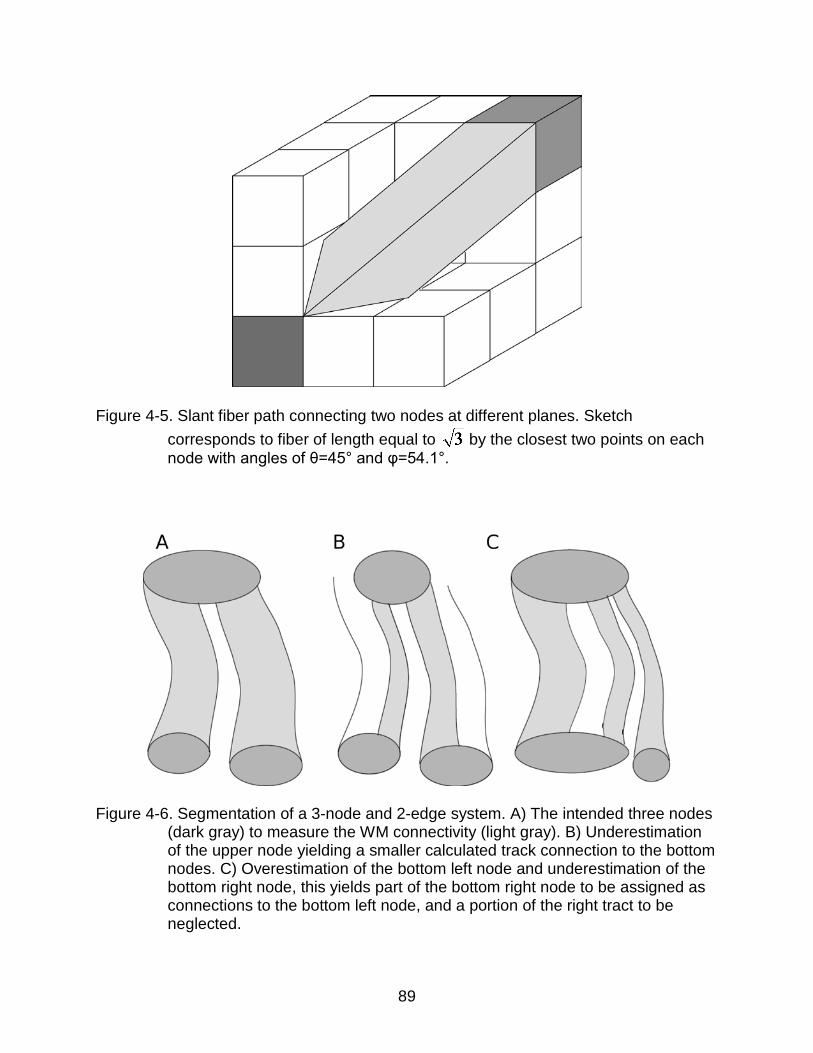
89
Figure 4-5. Slant fiber path connecting two nodes at different planes. Sketch
corresponds to fiber of length equal to by the closest two points on each node with angles of θ=45° and φ=54.1°.
Figure 4-6. Segmentation of a 3-node and 2-edge system. A) The intended three nodes
(dark gray) to measure the WM connectivity (light gray). B) Underestimation of the upper node yielding a smaller calculated track connection to the bottom nodes. C) Overestimation of the bottom left node and underestimation of the bottom right node, this yields part of the bottom right node to be assigned as connections to the bottom left node, and a portion of the right tract to be neglected.

90
Figure 4-7. Human and rat brain networks. A) Coronal view of the cingulum node.
B) Saggital view of the corpus callosum nodes. C) Saggital view of the cingulum network shows the disk nodes and the fiber connecting them. D) Coronal view of the CC network shows the disk nodes and the fiber connecting them. E) TL network at the interpolated resolution of 95 um. F) TL network with tracks connecting nodes at acquisition resolution of 190 um. G) TL network at the degraded resolution of 380 μm. H) Sketch of the TL simple graph; hippocampus, HC, thalamus, TH, amygdala, AM, and entorhinal cortec, EC (Color scheme is maintained in all figures). I) Coronal slice displaying the nodes.

91
Figure 4-8. System of 2 nodes connected by a fiber at 45 degrees from the pixels.
A) Color meanings; ROIs to be connected in dark gray, tract to be quantified in light gray and tiny dark squares are the seeds points. B) After keeping the seedpoints that lie within the region R, out of 36 original seed points, only 8 contribute to the edge weight.
Figure 4-9. Edge weight (Equation 4-6) plots of arc and slants of Figures 4-4 and 4-5.
A) Arc edge weight plateaus to: 0.167 for radius, r, of 1.5, 0.166 for r=2.5 and 0.165 for r=3.5. B) Slant in plane edge weight plateaus to: 0.234 for a separation of one voxel through its closest point, 0.233 for a separation of two voxels, and 0.233 for a separation of three voxels. C) 3D slant plateaus to: 0.284 for a separation of one voxel to its closest points, 0.282 for a separation of 2 voxels and 0.281 for a separation of 3 voxels.

92
Figure 4-10. Edge weight values for a slant in plane of single voxel nodes. The nodes
closest points were separated by; 1, 2, 3, 5, and 10 voxels.
Figure 4-11. Coefficient of variation (cv) plots as a function of σ levels and node
separation. The nodes closest points were separated by; 1, 2, 3, 5 and 10 voxels.

93
Figure 4-12. Edge weight plots for disk nodes in the cingulum and corpus callosum
tracts. A) Corpus Callosum disk nodes edge weights, B) cingulum disk nodes edge weights.
Figure 4-13. Excised rat brain edge weight values in the TL network. A) Left and,
B) right side TL edge weights. Values shown are across different resolutions of 95, 190 and 380 μm. TH-EC not displayed due to its small value.
Figure 4-14. Excised rat brain node strength values in the TL network. A) Left and
B) right side TL node strength values. Values shown are across different resolutions of 95, 190 and 380 μm.

94
Figure 4-15. Excised rat brain surface area values for the TL structures. A) Left and
B) right side TL node surface area measurement. Values shown are across different resolutions of 95, 190 and 380 μm. Segmentation was performed in the 95 μm data set and registered onto the 190 and 380 μm sets using FSL’s FLIRT and ApplyXFM.
Figure 4-16. Excised rat brain edge length values in the TL network. A) Left and, B) right
side TL edge lengths. Values shown are across different resolutions of 95, 190 and 380 μm. Observed fiber length differences in Fig. 7 are more pronounced on the TH-EC edge.

95
Table 4-1. Edge weight values across the acquired ten data sets of 1 mm3. The
proposed restriction, i.e. criteria 1 and 2, to obtain the fiber connecting fibers reduces the variation across different scans.
Edge (e) Proposed restrictive method Common approach, no restriction w(e) cv w(e) cv
CC (long) 1.33E-01 7.57% 9.42E-01 10.44% CC (short 1) 1.56E-01 9.29% 2.26E+00 13.09% CC (short 2) 1.79E-01 8.54% 2.77E+00 9.05% Cingulum (long) 6.12E-02 9.52% 2.56E-01 12.36% Cingulum (short 1) 7.66E-02 7.74% 5.64E-01 9.76% Cingulum (short 2) 8.87E-02 7.80% 7.02E-01 9.80% Table 4-2. Edge weight values across the acquired ten data sets of 8 mm3. The
proposed restriction, i.e. criteria 1 and 2, to obtain the fiber connecting fibers reduces the variation across different scans.
Edge (e) Proposed restrictive method Common approach, no restriction w(e) cv w(e) cv
CC (long) 9.62E-02 11.13% 6.06E-01 15.24% CC (short 1) 1.16E-01 9.55% 1.62E+00 15.01% CC (short 2) 1.33E-01 9.88% 1.95E+00 13.29% Cingulum (long) 4.31E-02 12.49% 1.50E-01 15.12% Cingulum (short 1) 5.75E-02 10.73% 3.57E-01 11.86% Cingulum (short 2) 6.26E-02 8.15% 4.06E-01 13.57%

96
CHAPTER 5 TOPOLOGY OF WEIGHTED BRAIN NETWORKS
5.1. Opening Remarks
Structural network studies generally use binary connectivity representations, in
which every connection between nodes is equivalent (Hagmann et al., 2007; Iturria-
Medina et al., 2007). Consequently in binary representations, the connection either
exists or does not exist. In reality, the brain is a heterogeneous system comprised of a
range of WM connection strengths (Catani et al., 2002; Concha et al., 2005). Also,
computational models of neural networks were proven to display enhanced
synchronizability using weighted networks (Chavez et al., 2005). Therefore, to account
for the enhanced behavior obtained from simulations of weighted computational models,
the analysis of network structures necessarily has to include a weighted connection
between nodes to describe brain networks. Because the relative “strength” of white
matter tracts in the brain varies, weighting the network is necessary to differentiate
between the network connections of various strengths (Butts, 2009). Additionally
weighting the edges of the network adds an extra degree of freedom to calculated
network parameters. Various weighted network parameters have been proposed in
literature, but a comprehensive weighted connectivity framework has not been proposed
that allows the estimation of topological traits of networks, such as those of a small
world (Watts and Strogatz, 1998) or a scale free (Barabási and Albert, 1999) network.
In this chapter, a generalization of the framework used to study brain network
organization is introduced then applied to determine the advantages that weighted
edges have on the calculated measures of network connectivity. The usual framework
used to estimate the topology of brain networks includes the calculation of the degree

97
distribution, path length and clustering coefficients (Watts and Strogatz, 1998). In
separate works, all of these calculations have been generalized to weighted networks.
With these generalized network measures the topological features (small world or scale
free organization) of brain networks are estimated using a weighted network. This
approach leads to a more realistic model of the brain network, which leads to a more
robust characterization of the network topology.
5.2. Methods
The procedures used to construct the human cortical networks are described in
this section. First the procedure to obtain the nodes is described and then the edge
assignment and weighting is reexamined from Chapter 4.
5.2.1. Network Construction
In brain networks created from tractography, thresholds are usually employed to
reduce the number of artifactual streamlines and the effects of volume averaging of the
voxels in network measures. In binary networks thresholding introduces two problems
into the networks calculations. The first is the arbitrary selection of the threshold and the
second issue that arises is that networks with different thresholds are not independent
samples (Langer et al., 2013). First, the arbitrariness of chosen thresholds does not
ensure that real edges are not eliminated or that artifactual edges are eliminated, since
there is not a clear criterion to achieve the elimination of artifactual streamlines. Also,
the statistical results obtained for all networks will depend on the selected thresholds.
Secondly, networks created at different thresholds are pseudo replicas of group level
networks (Langer et al., 2013). This means that the results obtained from the same data

98
expressed as a sparse network is also contained in a dense network, but not vice-versa.
This indicates that there is direct dependence of the calculated network properties on
the applied threshold, which leads to different results at different thresholds. In this
chapter, binary and weighted metrics are calculated for networks created at different
thresholds to determine whether weighting the network’s edges allows better estimation
of an appropriate threshold or if it is possible to eliminate it from the analysis.
Low edge weight values are commonly used as thresholds to eliminate what
could be considered artifactual edges connecting any two nodes. In binary networks,
sparse networks (i.e. the number of edges is much less than 30% of the total number of
possible edges) allow better estimation of the topological properties of networks,
because the nodes of dense networks become highly connected, almost leading to a
complete graph (every node connected to all others in the graph). Hence thresholds
also aid in the characterization of the topological properties of binary networks. In this
work, a high seed density (Pvoxel = 125) is used to maximize the accuracy of the
calculated edge weights, and the edge weight itself is calculated to reduce the effect of
artifacts (Section 4.3.1) (Colon-Perez et al., 2012). In this chapter, thresholds will be set
low enough so that “weak” edges are not removed just to create sparse networks. To
determine an appropriate threshold level, suppose that a characteristic “small” edge in
the brain network has a length of 3 mm and the streamline fibers are entirely contained
within three voxels. Using Equation 4-3, a total of 375 streamlines (M x P = 3 x 125 =
375) should be connecting the nodes; therefore, a threshold of 125 streamlines or more
would require that at least ~33% (i.e. 125 / 375) of all streamlines that potentially make
up the edge to be present. Consequently the number of streamlines connecting any two

99
nodes, and not the edge weight value, will be used as a threshold for the edges of the
brain network. As stated before thresholds are arbitrary, and this one is not the
exception. In this dissertation the number of streamlines will serve as the criterion to
compare results of network measures in binary and weighted networks constructed at
different thresholds. Considering the high volume of seeds per voxel used in this work,
three thresholds will be used to examine the effects of thresholding on calculated
network parameters. First, binary and weighted network parameters will be calculated in
networks without applying any threshold, i.e. any two nodes connected by at least one
streamline will have an edge. Then edges with 25, 50 and 125 or more streamlines will
be considered valid edges. In other words, 4 networks will be studied in this chapter;
one with no applied threshold (this will be referred as 0 threshold), then a threshold of
25, 50 and 125 streamlines or more making up an edge (these last three will be 25, 50
and 125 threshold, respectively).
An automatic segmentation algorithm called Freesurfer was used to define sets
of 68 anatomical nodes (Table 5-6 has a list of the nodes and their appropriate label
numbers used in the figures of this chapter) in all of the human data sets (Fischl, 2012;
Fischl et al., 2004). Freesurfer uses the T1 weighted images (i.e. structural images) to
register each structural image to an atlas of predefined anatomical brain regions. First
the algorithm removes the skull and creates an atlas of the white matter in the brain
(based on intensity values of each pixel in the structural image) to set the points that
determine the boundaries of the brain regions. This first step creates two brain
structures: WM, and everything else. The non-WM structure is ultimately segmented
into the predefined anatomical nodes in each brain. The structural image was then

100
registered to diffusion weighted images using FSL’s FLIRT (Jenkinson et al., 2002)
algorithm, using an affine transformation. The affine transformations include: rotations,
translations, and dilations and/or shears. Employing FLIRT’s transformation matrix
output, Freesurfer’s nodes were then registered from the T1 weighted image to DWI
using FSL’s ApplyXFM.
To avoid repetition the reader is referred to Section 4.2, which describes in detail
the procedure used to define each edge of the human cortical networks used in this
chapter. The edge weight as described by Colon-Perez, et.al.(Colon-Perez et al., 2012)
and Chapter 4 is used to estimate the connectivity strength of the edges in the network.
5.2.2. Null Hypothesis Graphs
The results of network metrics are influenced by the decisions made in creating
the network (e.g. number of nodes and edges, and the degree distribution). Therefore,
to test the significance of the brain network results (i.e. clustering coefficients and path
lengths) they are compared to results obtained for null hypothesis graphs. Null
hypothesis graphs of binary networks are formed by selecting edges at random with two
constraints: 1) the number of nodes and 2) the degree distribution remains identical to
the original brain network obtained for example by tractography. Since these graphs are
constrained by the number of nodes and the degree distribution, differences between
null hypothesis graphs and graphs obtained from brain networks are not due to local
differences in connectivity (i.e. node degree discrepancies) (Sporns, 2011).
Null hypothesis networks are employed in this study to determine the structural
organization and the topological traits of brain networks. Weighted null hypothesis
networks (like the ones to be described now) have not been described before. To create

101
weighted null hypothesis networks a third constraint is proposed to account for the
additional degree of freedom resulting from weighting the edges of the network. The
weighted null hypothesis networks will preserve the number of nodes, the degree
distribution (similarly to the binary case) and in the weighted case the edge weight
distributions of the original brain networks will also be preserved. The process of
creating null hypothesis graphs starts by storing lists of the edge weight values and the
node degree distribution (binary) for each brain network. Then, starting with the same
number of nodes as the brain network, the edges are assigned at random to connect
node pairs, with the restriction that the node degree distribution is preserved. As each
edge is assigned, simultaneously an edge weight is randomly selected from the edge
weight list and is applied to weigh the edges of the null hypothesis network. Ultimately,
this creates a random network (i.e. a weighted null hypothesis graph) with the same
node degree and edge weight distribution as the calculated brain network.
5.3. Network Metrics
The weighted edges require expanding the adjacency matrix to contain an extra
parameter that accounts for the strength in connectivity on each edge. The binary
adjacency matrix A, becomes the weighted connectivity matrix, A’ (Newman, 2010) and
the elements of the connectivity matrix are given by
. (5-1)
where w(eij) is the edge weight (Equation 4-6) defined in the section “Edge weight
Derived from DWI” (Section 4.2.2). The weighted connectivity will allow calculating
weighted network metrics analogous to the ones derived from the adjacency matrix
)(' ijijij ewaa ⋅=

102
(Section 2.2.1). The weighted connectivity matrix will become the foundation that allows
generalization of the framework that estimates the topological properties of weighted
networks (Watts and Strogatz, 1998).
5.3.1. Node Connectivity
The degree (Section 2.2.1) can be generalized to study weighted networks by
substituting the adjacency matrix with the weighted connectivity matrix, where the
element ij represents the strength of connectivity between nodes i and j. With the ability
to calculate the edge weight, the degree (Equation 2-6) can be generalized by
substituting the degree with node strength (Newman, 2001). The node strength (s(ni)) is
expressed as
. (5-2)
5.3.2. Average Weighted Path Length
Average path lengths reveal how effectively any node communicates with all of
the others in the network. A generalization of path length (Section 2.2.1) can be made
by the use of Dijkstra’s algorithm to find a single path between nodes i and j, where the
strongest path is used to connect any two nodes. Details of the algorithm can be found
in Introduction to Algorithms (Cormen et al., 2009). Essentially in weighted networks,
the algorithm searches for strong paths, i.e. the largest sum of edge weights connecting
any two nodes along any path with the least number of edges (there may be several
∑∑==
⋅==N
jijij
N
jiji ewaans
11)(')(

103
paths with the least number of edges). Equation 5-3 defines the average weighted path
length.
(5-3)
where plij represents the largest sum of edge weights traversed along the shortest path
between node i and node j. Networks may contain several shortest path, in such cases
the strongest path length is the path that yields the highest sum of the edge weights
along a shortest path. It is important to note that the path length in this context is not a
measure of Euclidean distance, i.e. the binary path length between any two nodes is not
the distance between their center of masses, but the number of steps it takes to connect
them (Equation 2-18). In the weighted framework, as stated before, the weighted path
length is the largest sum of edge weights along the shortest path. For example, in
Figure 5-1 the Euclidean distance from node a-c should be a path from a to c, since
these are not connected as a network plac = w(eab)+ w(ebc) ≠ w(eac). In a binary network,
the edge weight, w(eij) = 1, therefore plac = 2 since information has to travel from a to b
and then arrive at c.
The graph in Figure 5-2 will serve as a demonstration of Dijkstra’s algorithm. The
algorithm starts off with the weighted connectivity matrix as the estimation of the
strongest path for nodes connected by one edge, and the zero elements are estimated
with the strongest path connecting the nodes linked via two or more steps. To calculate
the weighted path from node n1 to n6 in Figure 5-2, the algorithm will find the lowest cost
by obtaining the highest sum of weights of the edges connecting n1-n6. The starting
node, n1, has three neighbors, two of which connect to n6. The algorithm compares pl16
1)(' 1
−=∑=
N
plnl
N
jij
i

104
experiencing the path, w(e13)+ w(e36) and w(e12)+ w(e26). From a visual inspection of
each path on Figure 5-2, it can be determined that w(e13)+ w(e36) > w(e12)+ w(e26):
therefore, pl16= w(e13)+ w(e36). This process is repeated in all zero elements of the
weighted connectivity matrix until all the [(N x (N-1)) / 2], paths are estimated with the
value of the strongest path connecting the nodes.
5.3.3. Clustering Coefficient
The clustering coefficient relates how well connected the neighbors of a node are
to the other neighbors of the same node. It provides some sense of the strength of the
communities formed around the nodes of the network. Multiple generalizations of the
clustering coefficient (Section 2.2.1) have been proposed in the literature, such as
Onnela, ci,O (Onnela et al., 2005) and Zhang, ci,Z (Zhang and Horvath, 2005). Saramaki
summarizes the properties among all weighted clustering coefficients, ci (Saramaki et
al., 2007). Saramaki et.al. concludes that there is not an all-purpose weighted clustering
coefficient. They argued that any network characterization should be made from two
perspectives: binary and weighted. In this dissertation two weighted clustering
coefficients will be used since there is no consensus on an appropriate weighted
clustering coefficient to study brain networks. The weighted clustering coefficients used
in this work are given by
, (5-4)
and
∑=−
=N
kjkijkij
iiOi ewewew
kkc
1,
3/1, ))(ˆ)(ˆ)(ˆ(
)1(1

105
, (5-5)
where
. (5-6)
These generalizations were chosen because they have the property that as ,
in all of the edges of a graph, the weighted clustering coefficient tends to , for any
triangle (i.e. three nodes fully connected between them). This ensures that the results in
weighted networks will yield the expected binary results as
5.3.4. Small Worldness
The last metric to be used is called small worldness (Humphries and Gurney,
2008). This metric takes the calculation of clustering coefficients and path lengths into
account and also considers the fact that small world networks deviate from random
networks predictions. Small world networks are “more” clustered and display more
“similar” mean path lengths than those predicted in Erdös’ and Rényi’s model (random
graphs called ER graphs, Section 2.2.2). Instead of using ER graphs in this chapter, null
hypothesis graphs are employed as control graphs to compare the brain networks. To
employ the small worldness parameter, the null hypothesis graphs will be analogous to
the ER graph, and the brain networks are analogous to the small world graphs
( )∑∑
∑
==
=
−
=
N
jij
N
jij
N
kjkijkij
Zi
ewew
ewewewc
1
22
1
1,
3/1
,
)(ˆ)(ˆ
))(ˆ)(ˆ)(ˆ(
))(max()(
)(ˆew
ewew ij
ij =
1)( , →jiew
1→ic
1)( , →jiew

106
described by Watts et. al (Watts, 2003). This null hypothesis network provides a better
comparison because the degree distribution and edge weight distribution are
maintained in both brain and null hypothesis networks. To calculate small worldness,
the ratio of the clustering coefficient (Equation 5-7) and average path length (Equation
5-8) for each network is compared with the null hypothesis graph.
(5-7)
where cg is the average clustering coefficient for a brain network and cN is the average
clustering coefficient for a null hypothesis network.
(5-8)
where lg is the average path length for the brain network and lN is the average path
length for the null hypothesis network. Finally, the parameter for small worldness, sw,
takes the form of the ratio of Equations 5-7 and 5-8, and is expressed as
. (5-9)
Real binary networks usually display γ > 1 and λ ~ 1, in this dissertation these
results are extended to weighted networks to estimate its organizational properties.
Binary small world networks present a high degree of connections among the neighbors
of any node when compared to a null hypothesis network, but the small average path
lengths are preserved. In weighted networks, these notions will be extended so that any
node will present a strong level of connectivity among its neighbors while the strong
path lengths will be preserved.
N
g
cc
γ =
N
g
ll
λ =
λγsw =

107
5.4. Results
In this section, the results of brain networks and null hypothesis graphs (Binary
and weighted) are summarized. The graph density, ρ, is defined as number of edges
divided by the total numbers of possible edges in the graph (from this point on any
reference to density will be specifically related to the aforementioned graph density
parameter). The minimum optimal graph density to determine small world organization
in brain networks derived from MRI has been studied before (Romero-Garcia et al.,
2012). It was found that an optimal graph density is roughly 8% and the maximum
calculated small worldness value was 2.38. As the number of nodes is increased, the
small worldness values increase due to a decrease in the density of edges in the graph.
This is due to the fact that at a larger number of nodes these become less likely to be
statistically correlated due to the reduced scale of the nodes (i.e. size of nodes). The
graph density will affect the binary metrics (described in the Networks Metrics section
2.2.1); such that as ρ 1, the path length and clustering coefficient will approach 1,
since most of the graph will be populated. Figure 5-3 shows how the graph density
changes for all 10 networks of a single subject (Section 3.1.1) as the thresholds
increase. The thresholding reduced the edge density from ~51% (0 threshold) to ~30%
(125 threshold) (Figure 5-3). This chart shows that the level of variation is consistent
across all networks with coefficients of variation (standard deviation/mean) of 3.5%,
3.7%, 3.7%, and 3.8% for networks created with the thresholds of 0, 25, 50, and 125
respectively. From this point on, the order of all comparisons across thresholds will be
shown from 0, 25, 50, to 125.
Average degree values are shown in Table 5-1 for all applied thresholds.
Average degree variations for each node on all ten networks at each threshold are

108
12.3%, 14.5%, 13.8%, and 13.9%. Figure 5-4 shows the average degree values for
each node, the bars represent the variation across the ten networks. Observing the y-
axis on Figure 5-4 and Table 5-1, one can see the changes in average degree
decreasing with the increasing threshold. This is expected since, as the threshold is
increased, it reduces the number of edges from ~51% (0 threshold) to ~30% (125
threshold) (Figure 5-3). The overall shape of Figure 5-4 was maintained at all thresholds
(i.e. the high degree nodes were the same at all thresholds). Since thresholds eliminate
“weak” edges, these connections appear to be distributed evenly within the entire
network. As was stated before, there are 68 nodes in the cortical network employed in
this chapter; for the sake of clarity, the nodes names will not appear in the figures as it
would make them too crowded and impossible to read. In this section the discussion of
specific nodes will be reserved for the nodes with extreme values, since discussing
each node result in detail would be too long and confusing to the reader. As the
threshold is changed, the node degree shows reductions from 0% (paracentral lobule
node, comparing node degree at 25 and 50 thresholds, this is the only node that did not
change degree from one threshold to the next) to up to 62% (frontal pole node,
comparing node degree at 0 and 125 thresholds). The nodes with the highest degree
across all thresholds are the left (L) parietal lobe (Label 28), the right (R) superior frontal
cortex (Label 62) and L superior frontal cortex (Label 27). The average node degree of
L parietal lobe is: 56.8, 47.1, 45.1 and 41.6, across thresholds. The average degree of
R superior frontal cortex is: 56.3, 43.6, 40.8 and 36.2, across thresholds. The average
degree of L superior frontal cortex is: 53.5, 43.3, 39.7 and 35.9, across thresholds. The
label numbers in parenthesis represent the nodes number in Figure 5-4. The removal of

109
“weak” edges reduces every node degree value (except for paracentral lobule
comparing the degree at 25 to 50 thresholds) at each threshold.
As the threshold is increased, “weak” edges are removed which reduces the
degree of the nodes connected by these weak edges. The biggest degree reductions,
on average, were found when comparing the degree of non-thresholded networks with
the thresholded networks: 28.4% (0 and 25), 34.0% (0 and 50), and 40.7% (0 and 125)
while thresholded networks showed a decrease of 7.7% (25 and 50), 17.5% (25 and
125) and 10.6% (50 and 125). To observe whether these networks display the scale
free characteristics of hubs, degree distributions on log-lin plots are shown on Figure 5-
5. A scale free network would display a long tail as the node degree increases, implying
the presence of high degree nodes, called hubs. This long tail is not observed; instead,
a sharp decay is observed at the highest degree. In other words, hub nodes are not
present in these networks. Consequently, the brain does not appear to display a
preferential attachment organization (i.e. scale free organization, Section 2.2.4)
agreeing with previous results employing tractography (Hagmann et al., 2007).
Average node strengths are shown in Table 5-2 for all applied thresholds. The
average node strength is constant and the variation is 9.6% at all thresholds. The node
strength’s uniformity across all thresholds is due to the edge weight value of weak
edges; on average these edges exhibited smaller edge weight values than the majority
of edge weights by more than 100 orders of magnitude. Therefore, eliminating these
small edge weights from the node strength calculation resulted in the small variations
observed in the node strength calculation as thresholds are increased. As the threshold
is changed, the node strength showed differences from 0% to 0.24%. Average node

110
strengths and variations (Figure 5-6) did not significantly change as the threshold was
varied. Although Figure 5-6 seems to display the same plot four times this not the case.
The changes in node strengths are so small that distinguishing the node strengths at 0
and 125 thresholds becomes almost impossible. This is in stark contrast with the degree
result (Figure 5-4) which displays clearly visible changes with changes in threshold.
Node strength distributions are displayed in Figure 5-7 and, as in node distribution, a
preferential attachment organization is not observed (i.e. power law decay). In Figure 5-
7 as the threshold is changed the node strength distribution is minimally affected, unlike
Figure 5-5. The node strength distributions indicate that thresholding does not have a
significant effect on node strength calculation using the edge weight (Equation 4-6). The
nodes with the highest node strength across all thresholds are the L insula (Label 34),
the R caudal anterior cingulate (Label 36) and the L posterior cingulate (Label 22). The
label numbers in parenthesis represent the nodes’ numbers in Figure 5-6. The average
node strengths of L parietal lobe, the R caudal anterior cingulate and the L posterior
cingulate are: 0.127, 0.125 and 0.123 respectively, across thresholds (the anatomical
location and shape of these nodes is shown in Figure 5-14). These nodes contain big
coherent WM tracks associated to their connectivity with the rest of brain. Quantitatively
these large tracks are represented with large edge weight values; hence the node
strength of the aforementioned nodes is increased by the presence of these large
pathways.
The changes in the binary and weighted adjacency matrices are shown in Figure
5-8. As the threshold is changed, the binary matrices display significant variation on the
adjacency matrices, while no noticeable difference is observed in the weighted

111
matrices. The highest edge weight values are observed as red points in the top-left and
bottom-right quadrant of the weighted connectivity matrices. These represent inter-
hemispheric connections between the L and R caudal anterior cingulate cortex (w(e) =
0.090, shown in Figure 5-15), the L and R medial orbitofrontal cortex (w(e) = 0.054,
shown in Figure 5-15) and the L and R rostral anterior cingulate cortex (w(e) = 0.054,
shown in Figure 5-15). These connections facilitate information transfer from the right to
the left side of the brain. The corpus callosum (large and coherent WM track) is the
main WM pathway associated with these connections, and as it has been said before,
large and coherent WM pathways are represented by large edge weight values.
Figure 5-9 displays the path length distribution for all thresholds and reveals that
the brain networks are organized in favor of shorter path lengths. As the thresholds
were increased the path lengths were also increased, this is seen in Figure 5-9 as shift
towards longer paths lengths as thresholds were increased. When the graph density is
high, weak edges serve as shortcuts in the network. At all thresholds, it was found that
all nodes had an average path length shorter than 2.5 steps, even when the
thresholding reduced the edge density by 20% from the 0 to 125 threshold (Figure 5-3).
Average path length values of the entire brain graph are shown in Table 5-2, which
ranges from 1.51 to 1.79, across thresholds. The node with the shortest path length was
the L superior parietal lobe (Figure 5-14) across all thresholds; 1.16, 1.31, 1.34 and 1.39
(from 0 to 125 thresholds respectively). The R superior frontal cortex displayed the
second shortest path length values with network of high density (0, 25 and 50
thresholds) with values of; 1.17, 1.36 and 1.41, while the L lateral occipital lobe
displayed the second shortest path length at the lowest density (125 threshold) with a

112
value of 1.48. Also displayed on Table 5-3 are the results of average path length for the
null hypothesis networks, which as expected display similar and slightly shorter path
lengths ranging from 1.50 to 1.72, across thresholds. The short path length found in this
work suggests an effective network organization for information traveling along the
edges of the network. The path required to deliver information in brain networks has to
only traverse a few nodes before reaching the recipient node, this ultimately reduces the
probability of information being distorted as it travels through the network.
A broad range of weighted path lengths was obtained as shown on Figure 5-10,
with values ranging from 8x10⁻⁴ to 3x10⁻³. Unlike node strength, the weighted path
length displays a higher vulnerability to thresholding and shifts the bulk of the
distribution to higher values, i.e. to stronger paths, as the thresholds are increased. This
effect can be observed as well in the strongest path lengths obtained at different
thresholds (Table 5-4). Removing weak edges did not had a significant modification to
the obtained node strengths (Table 5-2) and the weighted connectivity matrix (Figure 5-
8) since they only made small contribution to these parameters. The weighted path
length does not share the robustness as thresholds are change displayed by the node
strength and the weighted connectivity matrix. This is due because as weak paths are
removed these essentially get replaced by paths that lasted the thresholding process,
which finally leads up to significantly stronger path lengths. The effect of thresholding
becomes evident looking at the strongest paths at each threshold. The strongest path
lengths were: The R caudal anterior cingulate cortex at high graph densities (0 and 25
threshold), while L caudal anterior cingulate cortex displayed the highest value in the
50-threshold network, finally the transverse temporal cortex displayed the highest value

113
at low graph density (125 threshold). Table 5-4 shows that the means of the brain
network path lengths range from 1.08x10⁻³ to 1.57x10⁻³, while mean weighted path
lengths on the null hypothesis graphs range from 1.40x10⁻³ to 2.23x10⁻³, yielding larger
weighted path length values than the brain networks. The strong weighted path length
proposes that the brain is arranged in a way that enhances the pathway strengths. This
allows the use of strong pathways to transfer information within the edges of network in
addition to the already discussed short paths, quite possibly to reduce the possibility of
information distortion as it’s transferred between nodes.
Clustering coefficient distributions, shown in Figure 5-11, indicate that the brain
networks display a high level of clustering, ranging from 0.4 to about 1, across all
thresholds. The nodes with the highest clustering coefficient across all thresholds were
the L transverse temporal cortex and the L banks of the superior temporal sulcus, with
mean values all above 0.95 at all thresholds. Average clustering coefficient values of
the entire network are shown in Table 5-3, ranging from 0.74 to 0.63, while null
hypothesis results show means varying from 0.66 to 0.39. As the threshold increases,
the brain network displays a higher clustered organization than that observed in the null
hypothesis. In other words, the brain is arranged to allow enhanced communication
between communities of nodes (i.e. nodes sharing similar neighbors). The advantage of
high clustering is to allow regions that work together processing information, to achieve
faster results by being able to send and receive information directly to the regions
involved in the processing to achieve a function.
The distribution of the weighted clustering coefficients shows an interesting result
that is not present in the binary clustering coefficient distribution— it displays a slower

114
than exponential decay at all thresholds, similarly to the degree distribution of scale free
networks. In the clustering coefficient distributions, a few nodes are observed with a
very high level of clustering for both weighted clustering coefficients. Using the
clustering coefficient of Equation 5-4 (cO) the most clustered nodes were found to be the
L transverse temporal cortex, banks of the superior temporal sulcus and R transverse
temporal cortex respectively. At the highest graph density the banks of the superior
temporal sulcus becomes the third more clustered node while R transverse temporal
cortex becomes the second. On the other hand, using the clustering coefficient of
Equation 5-5(cz) the most clustered nodes are L and R banks of the superior temporal
sulcus and the parahippocampal gyrus, across all thresholds. Average weighted
clustering coefficients of the entire network can be seen in Table 5-4, ranging from 4.42
x 10-3 to 10.1 x 10⁻³ using cg,O and 5.25 x 10⁻³ using cg,Z at all thresholds. Table 5-4 also
shows the null hypothesis results, which display significantly smaller clustering
coefficients than those in the brain network. The null hypothesis cg,O results range from
1.04 x10⁻³ to 2.81 x10⁻³, and cg,Z at all thresholds is 1.82 x10⁻³. As expected the brain
displayed high clustering with weighted measures compared to null hypothesis
networks. The high clustering suggests that the brain is not a random network and that
it follows principles of advanced network structures (Watts and Strogatz, 1998). The
clustering coefficient, cg,Z, displayed little variation in its distribution as thresholds were
changed, similarly to node strength and the weighted connectivity matrix. From these
results one can reason that thresholds are not critical to construct weighted networks,
since differences from the null hypothesis are obtained in all graph densities.

115
Finally, the ratio, λ, of the brain network mean path length to null hypothesis
mean path length, and the ratio, γ, of the brain network mean clustering coefficient to
the null hypothesis mean clustering coefficient are shown in Table 5-5. As expected, the
binary network displayed γ > 1 and λ ~ 1 yielding sw > 1. This demonstrates the small
world property discussed in literature (Humphries and Gurney, 2008). The weighted
approach also displayed γ > 1 and λ ~ 1 yielding sw > 1, which shows the small world
property for the first time while employing a weighted network approach. The addition of
weighting (an extra degree of freedom) did not affect the measured topological small
world traits of brain networks, which further supports the idea that the brain is organized
as a small world and not as a scale free network. The structural networks follow a
physical topology, indicating that the connectivity of every node is limited by some
physical parameter. In the case of structural brain networks described here, the limiting
parameter is the surface area of the nodes. The scale free property implies an
extremely large connectivity for some nodes, but this is unrealistic for nodes limited in
the capacity to make connections. The binary networks did not display small world
topology in dense networks, due to the high density of edges in the graph. However,
weighted networks displayed small world topology at all thresholds, suggesting that the
small world property is an inherent property of the brain (when weighted) and not just for
sparse networks only. The weighing eliminates the restriction that networks should be
sparse to determine the topological organization of brain networks; in doing so the
thresholds are not necessary to determine the topological traits of brain networks.

116
5.5. Discussion
In order to increase the ability to have reproducible edges and edge weights, a
high seed density is used (Cheng et al., 2012b). The large number of seeds per voxel
(125) increases the possibilities of spurious connections and a high density of edges on
the brain networks. In order to cope with this, the edge weight from Chapter 4 is used to
ensure that the streamlines that connect the nodes meet the criteria for connectivity
discussed in Chapter 4. The results presented here support the idea that sparse graphs
in binary networks display a clearer small world organization than dense networks
(Humphries and Gurney, 2008). However, a more rigorous study of fiber tracking results
and their effect on the network density might answer the question of whether the real
brain networks displays low-density of edges, or if the real topology of brain networks
(those derived from tractography) includes a high-density of connections as reported
here. As shown in Figure 5-4, the degree variability across the ten networks is less than
15% for most nodes, while the node strength of most nodes variation is less than 10%
(see Figure 5-6). Utilizing a weighted approach reduces the variability in the average
connectivity parameter for each node (i.e. degree vs node strength) as thresholds are
changed (Figure 5-4 and 5-6). Another advantage of analyzing weighting networks can
be seen in the node strength across thresholds (Table 5-2), where the same values of
node strength is observed for graphs of high density (50% for 0 threshold) and low
density (30% for 125 threshold). By removing the edges with a low number of
streamlines, the analysis neglects the low edge weights, which only have values in the
order of 10-6, and are insignificant when compared to the bulk of the edges in the
network, which are in the order of 10-3. In other words, the thresholding in weighted
networks eliminates edge weights that are 100 to 1000 orders of magnitude smaller

117
than the majority of edges of the network. In the binary approach, since all edges are
given the same relevance, thresholding becomes a concern because the goal is to
eliminate spurious and artifactual streamlines, and the threshold would be the only
reasonable approach to eliminate the undesired connections that affect the network
measures. In node strength calculations, edges with small edge weight values
(compared with the mean edge weight values of the studied network) contribute
minimally to the final result, so the elimination of these edges will not significantly affect
the node strength calculations (Figure 5-6). Also, the visual representation of the
adjacency matrix (Figure 5-8) favors employing the weighted approach since
thresholding does not provide a significant contrast, in weighted matrices, with varying
thresholds. The removed edges have edge weights on the order of 10-5 and the largest
edge weight in the network is on the order of 10-2. Removing weak edges corresponds
to a reduction in the connectivity matrix on average, of less than 0.1%. In other words
substituting a value 10-5 by zero in a network where the highest edge weight is the order
of 10-2 does not affect substantially the visual appearance of the weighted connectivity
matrix (Figure 5-8). The binary network shows how the thresholding changes the overall
visual features of the adjacency matrix, while the weighted matrices did not display this
apparent behavior. The removed edges and edge weights are shown in Figure 5-14.
These plots show the differences as thresholds are increased; in the weighted matrix
the differences are negligible while in the binary matrix they are not. The weighted
differences are scaled by the largest edge weight removed; if the highest edge weight in
the network would have been used to scale it, these plots would appear as white (i.e. no
differences). Another advantage of weighting is that it easily distinguishes highly

118
weighted nodes and the important nodes connecting the hemispheres of the brain (the
top right and bottom left quadrants). Only a handful of nodes show a significant edge
weight value in Figure 5-8, while the binary matrices show a high density of edges.
These nodes (red points in Figure 5-8) are main anatomical domains that allow the
inter-hemispheric transfer of information. In the binary adjacency matrix this information
is lost due to the equivalency of the edges of the network.
The binary and weighted approaches did not show the same nodes with the
highest values of degree and node strength, which is easily explained by the emphasis
of each approach. The superior parietal and frontal cortexes displayed the largest node
degree values; these are fairly big nodes that have ample spatial occupancy within the
brain to create connections to all others nodes in the network (largest bars in Figure 5-
4). Also, these are association areas with multiple connections to and from primary
cortexes of the parietal and frontal cortexes respectively. On the other hand, the node
strength displayed high values for the insula, the caudal anterior and posterior cingulate
(largest bars in Figure 5-6, anatomical locations in Figure 5-14); these are nodes with
connections through the corpus callosum, which is the largest tract in the human brain.
These nodes with large node strength also contain large projections to subcortical
regions that in the weighted approach appear as strong edges connecting to other
cortical regions.
The brain networks were also found to be highly clustered as expected
(Hagmann et al., 2007), see Figure 5-11 and Table 5-3. However, as previously
described for binary metrics, the binary clustering coefficient is also highly susceptible to
thresholding. The weighted clustering coefficients displayed small variation across

119
thresholding (Figure 5-12, 5-13 and Table 5-4), similar to the node strengths. The
clustering coefficient described by Zhang (Equation 5-5) displayed a higher resilience to
thresholding than that described by Onnela (Equation 5-4). This might be a direct result
of Onnela’s normalization of the clustering coefficient by the node degree, k, which is
binary measure, while Zhang’s is entirely a weighted description of clustering. The
weighted approach also shows a slow decay in the log-linear plots of Figures 5-12 and
5-13, suggesting power law decay in the weighted clustering coefficient, and a small
collection of strongly clustered nodes. The banks of the superior temporal sulcus and
the transverse temporal cortex displayed high clustering coefficients values.
Anatomically these two regions serve as intermediary nodes of connected regions: the
superior temporal gyrus from the middle temporal gyrus and the primary auditory
regions, respectively. The parahippocampal gyrus resulted in a highly clustered node
employing Zhang’s clustering coefficient (Equation 5-5). Anatomically, this is a region
surrounding the hippocampus which also connects to perirhinal and entorhinal cortex.
These highly clustered regions serve as intermediaries to the brain functions associated
with the aforementioned areas. The weighted clustering coefficient displayed a larger
robustness than the binary clustering coefficient as thresholds are changed. This is
similar to the node strength argument that “weak” edges only minimally contribute to the
overall measure. The elimination of these edges does not significantly affect the
obtained results at high or low graph densities.
The binary path length was found to be “short” as predicted in references
(Hagmann et al., 2007). Thresholding increased the average path length, by virtue of
removing weak edges that serve as extra shortcuts in dense graphs. The weighted path

120
length was the weighted metric most susceptible to changes as the threshold was
changed, as shown in Figure 5-10. With the binary approach, the brain network showed
a higher average path length than the null hypothesis results. On the other hand, the
weighted approach exhibits lower average weighted path lengths in the brain network
than in the null hypothesis network. Higher values of the weighted path length should
not be seen as an increase in path length. Instead, they should be interpreted as
greater strength of the path. In binary networks, random organization leads to effective
paths between nodes (i.e. short distances between nodes). In the weighted approach,
random organization also shows effective paths between any two nodes by displaying
strong path lengths (i.e. high weighted path length values). The thresholding eliminates
weak paths, which have small weights throughout the pathway. These weak paths have
not been given any attention in brain network studies. This in part is due to the
thresholding used to remove them to be able to estimate topological properties of brain
networks. Nonetheless to estimate these weak ties, high seed densities in tractography
are necessary. Granovetter argued that weak ties are extremely important in social
networks, since it allows for the shorter path lengths observed in social interactions
(Granovetter, 1973). The same reasoning can be applied to brain networks, in that the
brain is organized in a dense mesh of nodes with a high number of edges that show an
intricate web of connections, weak and strong, providing a very stable network that is
very robust to random errors or attacks. Although sparse graphs improve our ability to
determine their topological traits, it could be possible that real networks might not be
sparse yet strict organizational features (small world or scale free) are still true. A node
with a large degree value implies that the nodes are connected through one edge to

121
many other nodes, yielding low path length values. Hence, binary networks with high
graph density will display what would seemingly be small world property (i.e. high
clustering and short path lengths) largely in part by virtue of high connectivity.
In weighted networks, nodes with the strongest weighted path length values were
highly affected by thresholding (Figure 5-10). Thresholding removes direct “weak”
connections between any two nodes; as the threshold is increased, weak and short path
lengths are replaced with longer and stronger path lengths. For example, as the
threshold is applied, if the resulting network is connected, then a “weak” direct (low
edge weight value) connection between any two nodes will be replaced by at least two
edges with “stronger” connections (larger edge weight values) than the original edge
weight. Consequently the new weighted path length will be significantly larger than the
original “weak” connection.
In the binary and weighted approaches the small world property in brain networks
was determined, as seen in Table 5-5. The binary network’s small worldness parameter
increased with a decrease in the density of edges, as expected, and the “small” small
worldness parameter in the binary unthresholded network is due to the high density of
edges in the network, ~50%. It comes as no surprise that the null hypothesis network
displayed small path length, but a high clustering was not expected. As the edge density
was high, the odds that the neighbors of any node were connected were high as well,
so the high clustering observed in the non-thresholded null hypothesis network is a
result of edge density and not of small world organization. Another advantage of
weighted networks can be seen in the displayed ranges of small worldness parameter,
sw, in Table 5-5. While binary networks only showed 1.53 for a thresholded network of

122
125, the weighted approach displays values of 5.13 and 4.10 for cO and cz respectively.
Therefore, a sharper small worldness organization is displayed in weighted networks.
5.6. Concluding Remarks
In multiple reports using a binary connectivity framework, the brain network
structure has been described as a small world network, which is dependent on the edge
density and the number of nodes (Bassett et al., 2011b; Hagmann et al., 2007; He et al.,
2009). The weighted connectivity approach provides a more stable framework to study
brain networks, since it adds a degree of freedom in the form of the edge strength. It
also provides an improved way to visualize the hubs and the inter-hemispheric brain
connectivity using just a simple display of the weighted adjacency matrix. Although all
binary metrics (degree, path length and clustering coefficient) were stable when
compared across acquisitions, when a comparison across thresholds (for all
acquisitions) was made, they varied significantly with graph density. The use of a
weighted network preserves the characteristic of small world organization and makes it
easier to determine brain topology. Observe that the range of small worldness (high
clustering and short path length) values in weighted networks was higher when
compared to the binary networks and the node strength distribution did not display
power law decay associated with scale free networks. Thresholds have significantly less
effect on the small worldness values in weighted networks (8% for cZ and 7% for cO,
Table 5-5) compared to the binary networks (28%, Table 5-5). The weighted network
approach provides higher connectivity values (strengths) when big pathways (like the
corpus callosum) connect the nodes, while the binary approach favors regions of large
volumes that contain multiple projections to other nodes. In binary brain networks,

123
nodes with large volumes will have many connections, even weak ones (i.e. small edge
weights); hence nodes will appear more connected (i.e. high degree), while in the
weighted networks, nodes with big white matter tracts associated to them will appear
more connected (i.e. high node strength). The major contributors to network variation in
both binary and weighted networks will be; volume averaging (due to limited spatial
resolution), subject variability, and node definition. Node definition is made carefully to
reduce its effect on calculated network parameters. Subject variability is the main
source to estimate differences in populations. Thresholding is commonly used to
mitigate the effects of artifactual streamlines due to volume averaging. However,
thresholding is an arbitrary procedure and the results of this chapter (Table 5) show that
thresholding is unnecessary to study weighted networks. Therefore weighted networks
reduce the number of possible sources of variation by one, by eliminating the need to
threshold the brain networks derived from tractography, improving the ability to obtain a
more realistic characterization of brain networks.

124
Figure 5-1. Three-node network connected by two edges. The distance from node a to
node c, is the sum of the distance from node a to b in addition to the distance of node b to c.
Figure 5-2. Eleven-node weighted network. Edge thickness represents the relative edge weight strength, e.g. e13 > e14.

125
Figure 5-3. Graph density plot. Density is obtained by taking the ratio of the number of
edges in a graph to the total possible number of edges in the graph.The threshold refers to the number of fibers required to remove an edge from the network. Zero refer to the unthresholded networks. Twenty five refers to networks constructed by eliminating edges made up by 25 or less fibers. Similarly for 50 and 125.

126
Figure 5-4. Node degree measurements. Plotted average values at different thresholds:
threshold 0 (top left), 25 (top right), 50 (bottom left) and 125 (bottom right). The changes in bar heights show the reduction in degree values for each node as the threshold is changed. Note that the y-axis on the 0 threshold network ranges from 0-60 while all others range from 0-50; the axis is not kept the same to allow better visibility of the degree values at all thresholds. See Table 5-6 for the list of nodes. The marks in all plots corresponds to the three largest degree values: (x) L parietal lobe (Label 28), (o) R superior frontal cortex (Label 62), and (+) L superior frontal cortex (Label 27).

127
Figure 5-5. Node degree distribution in log-linear scale. Plot threshold 0 (top left), 25
(top right), 50 (bottom left) and 125 (bottom right). The degree distributions are shifted towards lower degree values as the thresholds are increased.

128
Figure 5-6. Node strength values. Plotted average values at different thresholds
threshold 0 (top left), 25 (top right), 50 (bottom left) and 125 (bottom right). See Table 5-6 for the list of nodes. The brain networks displayed a reduction in the number of edges as the threshold was changed inducing a change in the degree values (Figure 5-4), conversely the node strenght do not show this evident change in the average values for all nodes since it in the order of less than 0.24%. The marks in all plots corresponds to the three largest node strengths: (x) L insula (Label 34), (o) L caudal anterior cingulate (Label 36), and (+) L posterior cingulate (Label 22).

129
Figure 5-7. Node strength distribution in log-linear scale. Plot threshold 0 (top left), 25
(top right), 50 (bottom left) and 125 (bottom right). Similar distributions at all thresholds suggest that the removal of weak edges only modifies minimally the node strengths obtained from network constructed at different thresholds.

130
Figure 5-8. Representative binary and weighted adjacency matrices. Binary plots on the
left and weighted plots right; thresholds at 0,25,50 and 125 from top to bottom. The binary matrices display stark differences as the threshold is increased, while weighted matrices seem exact replicas of each other. The red points corresponds to the larger edge weights in the entire network and anatomically these are inter-hemispheric connections traversing left-right in the brain.

131
Figure 5-9. Average binary path length distribution in log-linear scale. Plot threshold 0
(top left), 25 (top right), 50 (bottom left) and 125 (bottom right). As thresholds are increased the greater part of the distribution shift to larger path lengths, since shortcuts (“weak” edges) are removed from the network.

132
Figure 5-10. Average weighted path length distribution in log-linear scale. Plot threshold
0 (top left), 25 (top right), 50 (bottom left) and 125 (bottom right). As thresholds are increased the greater part of the distribution shift to stronger path lengths, since shortcuts (“weak” edges) are replaced with longer paths. The new paths will be two or more steps longer than the original “weak” path. Each edge that makes up the new path will have a larger edge weight than the original path, hence moving the distribution to stronger path lengths.

133
Figure 5-11. Binary clustering coefficient distribution in log-linear scale. Plot threshold 0
(top left), 25 (top right), 50 (bottom left) and 125 (bottom right). These plots show that as the threshold is increased the clustering coefficient distribution broadens. This implies that as “weak” edges are removed some nodes losses the strength of the communities around it but the overall the network still displays high values of clustering for most nodes (compared to null hypothesis networks, Table 5-3).

134
Figure 5-12. Weighted clustering coefficient (Equation 5-4) distribution in log-linear
scale. Plot threshold 0 (top left), 25 (top right), 50 (bottom left) and 125 (bottom right). Slight variations in the distributions can be observed as the threshold is change however the overall trend is maintained. The variation could be attributed to using a binary metric (degree) in this weighted measure.

135
Figure 5-13. Weighted clustering coefficient (Equation 5-5) distribution in log-linear
scale. Plot threshold 0 (top left), 25 (top right), 50 (bottom left) and 125 (bottom right). The clustering coefficient distributions seem to be replicas of each other as the threshold is changed, similar to the node strength and weighted connectivity matrices.

136
Figure 5-14. Anatomical location of human nodes. A) Superior parietal cortex, node with
high degree value. B) Caudal anterior cingulate, node with high node strength value. C) Frontal cortex, node with high degree value. D) Insula, node with high node strength value. E) Posterior cingulate, node with high node strength value.

137
Figure 5-15. Streamlines connecting nodes. A) Whole brain tractography map. B) Streamlines connecting the left and right rostral anterior cingulate. C) Streamlines connecting the left and right caudal anterior cingulate. D) Streamlines connecting the left and right medial orbito-frontal cortex.

138
Figure 5-16. Differences in binary and weighted matrices. Left column shows the binary
matrix changes as edges are removed with increasing threshold. Right column shows the weighted differences. Top row shows the difference between the unthresholded (0-threshold) and threshold of 25 streamlines or more (25-threshold). Middle row shows the difference between 0-threshold and 50-threshold. Bottom row shows difference between 0-threshold and 125-threshold.

139
Table 5-1. Average node degree ( k ) values (Equation 2-17) and standard deviation (σ). The values were averaged across the ten networks.
Threshold k σ 0 36.0 4.49 25 24.4 3.49 50 21.9 3.14 125 19.1 2.81 Table 5-2. Average node strength ( s ) values (Equation 5-2) and standard deviation (σ).
The values were averaged across the ten networks. Threshold s (10-2) σ (10-3) 0 6.88 7.40 25 6.88 7.40 50 6.88 7.40 125 6.88 7.40 Table 5-3. Binary path length and clustering coefficient metrics. The values were
averaged across the ten networks. Threshold lg lN cB,g cB,N 0 1.51 1.50 0.74 0.66 25 1.68 1.64 0.67 0.48 50 1.72 1.67 0.65 0.44 125 1.79 1.72 0.63 0.39 Table 5-4. Weighted path length (Equation 5-3) and clustering coefficient (Equation 5-4
and 5-5) metrics. The values were averaged across the ten networks. Threshold l’g (10-3) l’N (10-3) cO,g (10-3) cO,N (10-3) cZ,g (10-2) cZ,N (10-2) 0 1.08 1.40 4.42 1.04 5.25 1.82 25 1.28 1.65 7.51 1.96 5.25 1.82 50 1.37 1.89 8.46 2.30 5.25 1.82 125 1.57 2.23 10.1 2.81 5.25 1.82 Table 5-5. Small worldness of weighted and binary networks (Equations 5-7 through 5-
9). The γ and λ parameters were calculated from Tables 5-3 and 5-4. Binary Weighted (cO) Weighted (cZ) Threshold γ λ sw γ λ sw γ λ sw 0 1.13 1.01 1.12 4.24 0.77 5.51 2.89 0.77 3.76 25 1.39 1.02 1.36 3.84 0.78 4.95 2.89 0.78 3.72 50 1.47 1.03 1.43 3.68 0.73 5.08 2.89 0.73 3.99 125 1.60 1.04 1.53 3.61 0.70 5.13 2.89 0.70 4.10

140
Table 5-6. Human brain network nodes. The number in both hemispheres column correspond to the node placement in Figures 5-4 and 5-6.
Hemisphere Cortical region Left Right
1 35 Banks of the superior temporal sulcus 2 36 Caudal anterior cingulate 3 37 Caudal middle frontal 4 38 Cuneus 5 39 Entorhinal 6 40 Fusiform 7 41 Inferior parietal 8 42 Inferior temporal 9 43 Isthmus cingulate
10 44 Lateral occipital 11 45 Lateral orbitofrontal 12 46 Lingual 13 47 Medial orbitofrontal 14 48 Middle temporal 15 49 Parahippocampal 16 50 Paracentral 17 51 Parsopercularis 18 52 Parsorbitalis 19 53 Parstriangularis 20 54 Pericalcarine 21 55 Postcentral 22 56 Posterior cingulate 23 57 Precentral 24 58 Precuneus 25 59 Rostral anterior cingulate 26 60 Rostral middle frontal 27 61 Superior frontal 28 62 Superior parietal 29 63 Superior temporal 30 64 Supramarginal 31 65 Frontal pole 32 66 Tempora lpole 33 67 Transverse temporal 34 68 Insula

141
CHAPTER 6 PATHOLOGICAL NETWORKS
6.1. Opening Remarks
The goal of this Chapter is to use the edge weight (Chapter 4) and weighted
framework (Chapter 5) to study brain networks and show the favorability of weighted
networks to provide additional information to differentiate control brains from thyroid
disrupted (TD) networks. The thyroid hormone (TH) deficiency model is ideal since the
structural changes in the brain are due to changes in WM volumes, which in turn lead to
a decrease in the strength of connectivity measures.
With cocaine hypersensitivity (van der Marel et al., 2013), the rat brain has been
shown to display changes in connectivity. Using DTI, van der Marel et al. were able to
determine the small world organization in the rat brain using a weighted network.
However, their approach employed diffusion tensor imaging (DTI), used only 10 seeds
per voxel for the tractography, and weighted the network connections by FA values. A
problem with this approach is that DTI fails to estimate fiber crossings and kissing,
inducing errors in the connectivity map. The FA calculation is influenced by acquisition
schemes (Alexander et al., 2001; Jones et al., 1999), and present a problem in WM
regions where more than one fiber population crosses a voxel. In these regions, where
each voxel contains multiple fibers, the obtained FA values resemble a GM region even
though they are WM regions.
The results to be discussed in this chapter regarding rat brain organization
support van der Marel’s observation of small world organization in the rat brain. Also,
this weighted framework can be used to study brain networks of rats with changes in

142
connectivity (Powell et al., 2012) and disconnection syndromes (Catani and Ffytche,
2005).
6.2. Methods
6.2.1. Animals Treatment
The rat treatments were performed at the University of South Florida (USF, St.
Petersburg, FL) with the approval of the USF Institutional Animal Care and Use
Committee (IACUC) permit #R3486. Offspring of rat dams were randomly selected and
assigned for group treatments. For specific details of this procedure refer to Powell,
et.al.(Powell et al., 2012). The groups in this publication are control rats (n = 5) and rats
treated with 10 ppm 6-propyl-2thiouracil (n = 4) (PTU; Sigma Aldrich Corp, St. Louis,
MO). Dosing began at gestation day 7 and continued until postnatal day 25. Rats were
allowed to live until 90 days after birth, and were then sacrificed and perfused with
phosphate-buffered saline (PBS), followed by 10% buffered formalin phosphate (Fisher
Scientific Inc., Hampton, NH). Brains were removed from the skull and stored in formalin
for ex vivo imaging. Throughout the rest of this text, rats treated with PTU will be
referred to as PTU.
6.2.2. Networks
Using a digitized Paxinos atlas (Paxinos and Watson, 1998) a total of 40 rat
cortical nodes (Table 6-6 for the nodes names and their appropriate label number used
in the figures of this chapter) were defined. FSL’s FLIRT was used to register the
Paxinos atlas regions as nodes in diffusion space. Networks were constructed using the
methods outlined in Chapters 4 and 5. In this Chapter for each rat brain, two networks
will be created at different thresholds to estimate the organizational features of the rat

143
brain. The threshold will be employed to reduce the graph density and compare the
topological properties of rat’s brains in dense and sparse networks. Both networks will
contain the same number of nodes, but the edges will be defined in the first network by
having at least one fiber connecting any two nodes and the second will be with edges
made up of 6000 fibers or more. These thresholds will allow the comparison of dense
networks, i.e. high number of edges (~76% and ~70% of all possible edges in control
and PTU networks respectively) and sparser networks (~24% and ~21% of possible
edges in control and PTU networks respectively). Throughout the rest of this text, dense
networks of control rats will be referred to as DeCo (Dense Controls), sparse networks
of control rats will be referred to as SpaCo, (Sparse Controls), dense networks of PTU
rats will be referred to as DePtu, and sparse networks of PTU rats will be referred to as
SpaPtu.
6.3. Results
Null hypothesis networks allow determining whether any real-world network
displays any organizational feature different from a random network. In this section the
results of brain networks and null hypothesis graphs are summarized and a discussion
of the results will be provided in section 6.4. As a reminder, the graph density is the
number of edges present in the network divided by the total numbers of possible edges
in the graph. The PTU treated rats displayed a significant reduction in average degree
values in dense (p = 5.5 x10⁻⁴) and sparse (p = 1.6 x10⁻³) networks, as shown in Figure
6-1. Table 6-1 shows the average degree value of the entire network for control and
PTU brains. DePtu networks displayed a reduction of high degree nodes, as shown in
the degree distributions of Figure 6-2, which demonstrate a decreased connectivity on
PTU brains. The TD connectivity reduction can also be observed in the large number of

144
small degree values (Figure 6-2) compared to the normal networks. SpaPtu networks
displayed a faster decay of high degree nodes, as shown in the degree distributions of
Figure 6-2, implying a reduction in the overall connectivity in the network similar to the
dense network result. Similarly to Chapter 5, for the sake of clarity, the nodes’ names
will not appear in the figures as it would make them too crowded and impossible to
read. In this section the discussion of specific nodes will be reserved for the nodes with
extreme values, since discussing each node result in detail would be too long and
confusing to the reader. The nodes with the highest degree in the dense networks were:
DeCo—left (L) anterior cingulate (Label 21) (36.0), right (R) anterior cingulate (Label 1)
(36.0) and the R somatosensory primary cortex (Label 16) (35.9), while in DePtu
networks, they were: L retrosplenial cortex (Label 35) (36.5), L gustatory cortex (Label
26) (35.0) and R piriform cortex (Label 12) (34.8). However, in sparse networks the
nodes with the highest degree were: SpaCo— L somatosensory primary cortex (Label
36) (17.1), R somatosensory primary cortex (Label 16) (15.7) and R anterior cingulate
(Label 1) (15.1), while in SpaPtu, they were: L retrosplenial cortex (Label 35) (17.0), R
piriform cortex (Label 12) (14.3), and R retrosplenial cortex (Label 15) (13.3).
Average node strength of PTU rats displayed a significant reduction compared to
control brains in dense (9.8 x10⁻¹⁰) and sparse networks (p = 1.6 x10⁻¹⁰), as shown in
Figure 6-3. Table 6-2 shows average node strengths of PTU and control networks.
Dense and sparse networks displayed similar node strength values with a reduction in
the order of 10-3. Like degree distributions, node strength distributions indicate a
reduction in the number of strongly connected nodes (i.e. large node strength values).
The degree and node strength distribution graphs of both dense and sparse PTU

145
networks failed to exhibit a long tail, suggesting that no hubs are present; therefore, a
scale free organization is absent. The control network nodes with high node strength
values were: L orbital cortex (Label 31) (DeCo = 5.26x10⁻², SpaCo = 4.66x10⁻²), R
orbital cortex (Label 11) (DeCo = 4.81x10⁻², SpaCo = 4.28x10⁻²), and the third strongest
node in the DeCo network was the L infralimbic cortex (4.10 x 10⁻²), while in the SpaCo
network the third strongest was the L piriform cortex (Label 32) (3.83 x 10⁻²). Meanwhile,
the PTU network nodes with high node strength values were: R orbital cortex (Label 11)
(DePtu = 4.89x10⁻², SpaPtu = 4.12x10⁻²) L orbital cortex (Label 31) (DePtu = 4.35x10⁻²,
SpaPtu = 3.79x10⁻²) and the L gustatory cortex (Label 26) (DePtu = 3.80x10⁻², SpaPtu =
3.66x10⁻²). In Figure 6-5 the anatomical location of some of the nodes is shown.
The binary clustering coefficient of PTU dense networks presented a significant
reduction in clustering coefficients values, (p = 2.96 x10⁻¹⁰); however, the sparse
networks did not show a significant difference (p = 0.242). The clustering coefficient
distribution (Figure 6-4) shows an overall reduction in clustering values, with the normal
network displaying higher clustering than the PTU networks. Average clustering
coefficient values for binary networks, over the entire network (Table 6-3), showed a
high level of clustering (compared to null hypothesis networks) in dense and sparse
networks, while null hypothesis networks only showed a high level of clustering in dense
networks. The control networks displayed a high level of clustering for the following
nodes: DeCo—R somatosensory secondary cortex (0.95), L somatosensory secondary
cortex (0.92) and the R cortical amygdala (0.92), while in SpaCo, they were: R cortical
amygdala (1.00), L cortical amygdala (0.85) and L somatosensory secondary cortex
(0.78). Conversely, PTU networks displayed the following nodes with a high level of

146
clustering: DePtu— the R cortical amygdala (0.95), L temporal cortex (0.89) and the R
insular cortex (0.89), while the SpaPtu displayed the following: the R cortical amygdala
(1.00), L cortical amygdala (1.00), and L parietal cortex (0.83).
PTU networks display an increase on the average shortest path length in dense
(p = 6.77 x 10⁻⁴) and sparse (p = 1.71 x 10⁻⁵) networks. The average shortest path
length for PTU and controls was found to be similar to its value in comparable null
hypothesis networks (Table 6-3). The shortest path lengths in control networks were
associated to the following nodes: DeCo—R anterior cingulate (1.10), L anterior
cingulate (1.10) and the R somatosensory primary cortex (1.10), while in SpaCo, they
were: L somatosensory primary cortex (1.67), L piriform cortex (1.69) and the R piriform
cortex (1.70). Shortest path lengths on PTU networks were found with the following
nodes: DePtu—L retrosplenial cortex (1.09), the gustatory cortex (1.13), and the L
piriform cortex (1.13), while in the SpaPtu, they were: L retrosplenial cortex (1.60), the
piriform cortex (1.69), and L anterior cingulate (1.84).
The PTU networks displayed a significant reduction in weighted clustering
coefficient values (using Equation 5-5) in dense (p = 1.02 x 10⁻⁸) and sparse (p = 9.85 x
10-8) networks, as shown in Figure 6-4 and Table 6-4. The PTU networks using
clustering coefficient of Equation 5-4 also displayed a significant reduction in dense (p =
9.09 x 10⁻³) and sparse networks (p = 2.32 x10⁻³) (see Table 6-4). With both measures,
brain networks (PTU and controls) displayed a higher level of clustering than null
hypothesis networks. Both dense and sparse weighted brain networks displayed higher
clustering values than the null hypothesis networks, in contrast to the binary clustering
coefficient, which only displayed higher clustering in sparse networks. This high

147
clustering indicates that the network organization in the rat brain maximizes local
connectivity, which is not affected by TD. The highest clustering coefficient values
(using Equation 5-5) in control networks were associated to the following nodes:
DeCo—L tenia tecta cortex (0.27), R cortical amygdala (0.25) and L infralimbic cortex
(0.24), while in SpaCo, they were: L tenia tecta cortex (0.40), R tenia tecta cortex (0.29),
and the L infralimbic cortex (0.26). Conversely, the PTU networks displayed high levels
of clustering using Equation 5-5, for: DePtu – R tenia tecta cortex, R cortical amygdala
and L cortical amygdala, while in SpaPtu, they were: R tenia tecta cortex (0.37), L tenia
tecta cortex (0.25), and the R cortical amygdala (0.25). In contrast Equation 5-4 yielded
the highest values for the following nodes: DeCo—L orbital cortex (2.55 x 10⁻²), R
insular cortex (2.50 x 10⁻²), and the R somatosensory secondary cortex (2.49 x 10⁻²)
while the SpaCo network displayed: R cortical amygdala (2.51 x 10⁻¹), L cortical
amygdala (1.60 x 10⁻¹), and L orbital cortex (1.52 x 10⁻¹). Conversely, PTU brain
networks displayed the highest clustering levels using Equation 5-4 for the following
nodes: DePtu—L orbital cortex (2.28 x 10⁻²), R orbital cortex (1.79 x 10⁻²), and the L
temporal cortex (1.57 x 10⁻²), while in SpaPtu, they were: R cortical amygdala (3.02 x
10-1), L cortical amygdala (2.10 x 10⁻¹), and L orbital cortex (1.46 x 10⁻¹).
PTU networks showed a reduction of weighted path lengths in dense and sparse
networks; however, only dense networks display statistical significance (p = 1.06x10⁻⁹).
Null hypothesis networks showed similar path length values as in both dense and
sparse brain networks (Table 6-4). The strongest path lengths in control networks were
associated to the following nodes: in DeCo they were: L orbital cortex (1.32 x 10⁻²), R
anterior cingulate (1.20 x 10⁻²) and the L infralimbic cortex (1.07 x 10⁻²), while in SpaCo

148
they were: R cortical amygdala (7.00 x 10⁻²), L cortical amygdala (5.41 x 10⁻²) and the L
orbital cortex (5.20 x 10⁻²). Strongest path lengths on PTU networks were found with the
following nodes: in DePtu they were the following: R orbital cortex (1.22 x 10⁻²), the L
orbital cortex (1.09 x 10⁻²), and the L gustatory cortex (0.95 x 10⁻²), while the SpaPtu
were: R cortical amygdala (7.34 x 10⁻²), the L cortical amygdala (6.09 x 10⁻²), and L
orbital cortex (5.84 x 10⁻²).
As seen in Figure 6-2, rat brain networks did not display a scale free
organization. The clustering coefficient and path length results suggest non-random
organizational features in the rat brain. Small worldness values, shown in Table 6-5,
support the idea of small world organization in rat brains. Dense networks only show sw
values of 1.03 and 1.04 for normal and PTU brains, respectively. On the other hand,
sparse networks displayed values of 1.87 and 2.21 on normal and PTU networks. All
weighted measures displayed sw values larger than 3.3 in all networks, PTU and
normal, as well as dense and sparse, indicating more clearly organizational features of
efficient networks using the weighted framework.
6.4. Discussion
In this study, cortical nodes were defined as network nodes, and streamlines
calculated from tractography were defined as the network edges. Thyroid disruption
has been shown to affect WM volumes and brain structure with volumetric analysis
(Powell et al., 2012). This study shows that the changes with TD reduce brain
connectivity; however it does not eliminate the organizational features of small world.
Control and PTU networks displayed a linear decay in the degree distribution of sparse
networks, suggesting that no scale free organization is present in rat brains. The degree

149
distribution suggests that TD reduces the overall connectivity in PTU brains. The most
connected nodes (i.e. high degree) suggest TD prompts brain reorganization. Control
networks display high degree values for anterior cingulate (Figure 6-5) and the
somatosensory primary cortex (Figure 6-5), while PTU networks display high values in
retrosplenial cortex and piriform cortex (Figure 6-5). The changes in the nodes with the
highest degree suggest changes in organization upon TD, to maintain a high level of
connectivity in the network. The values of high degree nodes were similar in control and
PTU networks, with an overall reduction in the number of edges, hence a reduction of
degree values, throughout the entire network. The nodes with highest degree values
change on control and PTU networks; this can be interpreted as network reorganization
in TD brains to maintain features of normal brains, like high connectivity.
Node strength values display a larger significant difference (controls vs PTU)
than the degree values, which clearly supports previous findings of changes in brain
structure due to WM loss. PTU brains display similar node strength distribution to
control brains with an overall reduction in strength of connectivity throughout the entire
network. Unlike degree, nodes with high strength values were the same in control and
PTU networks; hence, the reduction in their value, agrees with the observation that WM
volume is reduced in PTU brains (Powell et al., 2012). In this case, brains still maintain
strong connection to the L and R orbital cortex (Figure 6-5 and 6-6), with reduction in
the WM integrity (i.e., node strength) due to TD.
Organizational features of brain networks can be determined with the use of
weighted network metrics. The clustering coefficient is related to specialized functions
(e.g. visual, olfactory, and so forth). Control and PTU brains displayed a high level of

150
clustering in sparse networks (Table 6-3); however, dense networks displayed similar
clustering results as the null hypothesis network. The high clustering in the dense null
hypothesis network is due to the high number of edges, which artificially increases its
overall clustering. Therefore, this is not due to organizational features in the null
hypothesis or lack of it in the brain networks. The PTU dense networks displayed a
significant difference in the binary (not weighted) measure of clustering from normal
brains. The changes in clustering were not significant in sparse binary networks as
weak edges were removed by thresholding. This can be attributed to changes in degree
values; the average number of edges was reduced by 6% in dense networks, and 3% in
sparse networks. The high clustering of brain networks that allow for specialized tasks is
maintained with high graph densities (in weighted networks as shown Chapter 5 and 6)
or TD (in sparse binary networks and weighted networks Section 6.3). The cortical
amygdala displayed a high level of clustering in all networks, while the somatosensory
secondary cortex displayed a high level of clustering in control networks. PTU networks,
displayed a high level of clustering in the temporal and insular cortex (Figure 6-6) in
dense networks and the parietal cortex in sparse networks. The graph density
dependence of highly clustered nodes in the PTU networks is due to a high number of
weak edges connecting the neighboring nodes of temporal and insular cortex, while
stronger edges are associated to the parietal cortex neighborhood.
The path length displays similar values in brain and null hypothesis networks.
This suggests an efficient brain organization that minimizes distances in the brain and
this property is maintained even with TD. The somatosensory primary cortex and the
anterior cingulate displayed small path lengths in DeCo networks while the
151
somatosensory and piriform cortex did so in SpaCo networks. Thresholding reduces the
connections that allow anterior cingulate to display small path lengths. This implies that
weak edges aid the anterior cingulate to achieve a high connectivity with the rest of the
network, while the piriform cortex exhibits the smaller path lengths in SpaCo networks
implying that stronger edges are connecting the piriform cortex to the rest of the
network. The retrosplenial and piriform cortexes displayed small path lengths in both
PTU networks (dense and sparse). The gustatory cortex displayed small path length in
dense networks, while the anterior cingulate displayed small path length in sparse
networks. The piriform cortex display showed small path lengths in all networks (DeCo,
DePtu, SpaCo, and SpaPtu) suggesting that is an important node in rat brain. The
piriform cortex is related to olfaction an important function for the rat. The rat does not
have a good vision, but does have a great sense of smell. Therefore, it is logical to
hypothesize that the rat brain is primed to protect the connectivity to and from its
olfaction centers to enhance its survival.
The weighted approach also displayed non-random organization in rat brains.
Unlike the binary clustering coefficient, the weighted clustering coefficient was able to
demonstrate higher levels of clustering in dense brain networks compared to null
hypothesis networks. It also displayed significant differences between PTU and normal
brains at high and low densities. Control brain networks displayed a high level of
clustering, using Equation 5-5 (Zhang), for the tenia tecta (Figure 6-5) and the
infralimbic cortex (Figure 6-6), while in PTU networks, the high levels of clustering were
displayed by the tenia tecta and the cortical amygdala. The cortical amygdala was also
a highly clustered node in control brains, but only for dense networks. The tenia tecta

152
appeared to have strong connections between its neighbors, even with TD; however,
the infralimbic cortex seems to have lost some of the strength associated with the
connections of its neighbors with TD. Meanwhile, using Equation 5-4 (Onnela) the
orbital cortex appears as the most clustered node in control networks, the
somatosensory secondary and insular cortex display high levels of clustering on dense
networks and the cortical amygdala does so in sparse networks. PTU networks display
the orbital cortex as a clustered node as well, with the temporal cortex also displaying
high levels of clustering at dense networks; finally the cortical amygdala does so at
sparse networks. The case of sparse networks showed the same nodes with the highest
clustering, with these displaying a reduction in their clustering coefficient values. The
most clustered nodes, the tenia tecta, cortical amygdala and orbital cortex are
associated with olfaction, memory and sensory integration, respectively. The high
clustering of these nodes suggests an organization placing them as mediators to the
aforementioned functions, which are of vital importance.
Lastly, the weighted path lengths displayed similar values in brain networks
compared to null hypothesis, suggesting that the brain creates strong path lengths
(pathways with large values of Equation 5-3) to maximize the presence of robust
pathways in the brain. Weighted path length differences, from control to PTU brains
gained statistical significance only on dense networks. The node with the strongest path
lengths in dense networks was the orbital cortex, with the anterior cingulate and
infralimbic cortex displaying strong values in controls, while the gustatory cortex (Figure
6-6) did so in the PTU brains. This suggests a reorganization reducing the strength of
connectivity of the anterior cingulate and infralimbic structures upon TD.

153
Brain network and null hypothesis differences suggest an efficient, small world
organization in the rat brain. Small worldness values are presented in Table 6-5,
displaying larger sw values in all of the weighted networks than in the binary networks.
Also, in binary networks only the sparse ones displayed sw values indicative of small
world organization. Graph density affects the determination of topological features of
networks at high values. So, arguably, the similar topological features of brain networks
and null hypothesis networks at high density in binary networks are artifacts of the high
density and the fact that all edges are equivalent in the binary approach. With binary
networks, it is not possible to determine the small world property of brain networks at
high graph densities. However using weighted networks described in this dissertation
(Chapters 4 and 5) the small world property is obtained for even high graph densities.
The ability to determine structural organization at high graph densities is due to the
heterogeneity in the edge weights, which are efficiently organized to allow strong
clusters and strong path lengths. This efficient organization is evident by calculating
weighted clustering coefficients and path lengths at high graph densities.
6.5. Concluding Remarks
In this Chapter the small world organization in the rat brain was successfully
determined. As expected, TD brains displayed reductions in connectivity and strength of
connectivity. However, small world organization of rat brains was still present even after
TD. Previous studies have shown deformities in WM and GM in rats’ brains with thyroid
hormone deficiencies (Powell et al., 2012). These deformities cause changes in brain
structure in the form of reduced WM volumes and heterotopias (presence of GM in
abnormal WM locations) in the corpus callosum. Rat brains with TD displayed reduced

154
global connectivity and strength of connectivity, implying that thyroid disruption reduces
the brain connectivity by means of inhibited connectivity (reduced degree) and
reductions of WM volumes, as shown by Powell (Powell et al., 2012) (reduced node
strength). The strongest and most connected nodes in normal and PTU brains were not
the same, suggesting that the WM reduction observed by Powell et al. (Powell et al.,
2012) is not a global reduction but probably is accompanied by reorganization to make
up the reduced WM tracks in the brain. A small sample was used in this study, possibly
more brain samples than the ones described in this chapter and additional analysis (e.g.
histology) should be made to fully support this claim. Since plasticity is a property of the
brain, it should be expected that the brain would attempt to make up lost WM volumes
to optimize its structure and display optimal network properties (the proof of this
statement should be treated in future work). The high clustering coefficient and short
path lengths obtained for PTU networks suggest that the reorganization is guided to
maintain high connectivity in the network, which allows the brain to properly function.
Basically, the brain reorganized to still allow an efficient communication in the entire
network (small and strong path lengths) with high local connectivity to allow the complex
functioning of brain regions (high clustering coefficients).
Even though it was found that there are structural changes associated with TD,
the entire picture is not complete if one does not understand the functional changes
associated with structural changes in the brain. In Chapter 7, a roadmap to merge the
structural results of this dissertation (Chapter 4-6) will be shown with models to study
the function in the brain.

155
Figure 6-1. Degree values, results of rat networks. Top-left plot, normal and sparse
networks. The marks correspond to the largest degree values: (x) L somatosensory cortex-node 36, (o) R somatosensory cortex-node 16, and (+) R anterior cingulate-node 1. Top-right plot, PTU and sparse brains. (x) L retrosplenial cortex-node 35, (o) R piriform cortex-node 12, and (+) R retrosplenial cortex-node 15. Bottom-left, normal and dense networks. (x) L anterior cingulate-node 21, (o) R anterior cingulate-node 1, and (+) R somatosensory cortex-node 16. Bottom-right, PTU and dense networks. (x) L retrosplenial cortex-node 35, (o) L gustatory cortex-node 26, and (+) R piriform cprtex-node 12. The first twenty nodes represent the right side of the brain and the latter twenty represent the left side of the brain.

156
Figure 6-2. Degree distribution (log-lin) of rat brain networks. Top-left plot, normal and sparse networks. Top-right plot, normal and dense networks. Bottom-left, PTU and sparse brains. Bottom-right, PTU and dense networks.

157
Figure 6-3. Node strength results of sparse networks. Top- left, node strength values of
normal networks. The marks corresponds: (x) node 31, (o) node 11, and (+) node 32. Bottom-left, node strength values of PTU networks. The marks corresponds: (x) node 11, (o) node 31, and (+) node 26.The first twenty nodes represent the right side of the brain and the latter twenty represent the left side of the brain.Top-right, node strength distribution (log-lin) of sparse and normal networks. Bottom-right, node strength distribution of PTU brains.

158
Figure 6-4. Clustering coefficients distribution (log-lin) of sparse networks. Top-left,
distribution of binary clustering coefficient of normal sparse networks and bottom-left, of PTU brains. Top-right, weighted clustering coefficient (cZ) distribution (log-lin) of normal sparse networks and bottom-right, PTU networks.

159
Figure 6-5. Anatomical location of rat nodes. A) Tenia tacta, node with high clustering coefficient values. B) Anterior cingulate, node high degree values in control brains. C) Orbital cortex, node with high node strength values in control brains. D) Piriform cortex, node with high degree values in PTU brains. E) Somatosensory cortex, node with high degree values in controls.

160
Figure 6-6. Streamlines connecting nodes in the rat brain. A) Whole brain tractography map. B) R gustatory cortex connected the R insular cortex. C) L gustatory cortex connected the L insular cortex. D) L infralimbic cortex connected to the L orbito-frontal cortex

161
Table 6-1. Average degree ( k ) values and standard deviation (σ). PTU networks display reduction in mean values while maintaining similar high and low degree values. Standard deviation k σ DeCo 29.4 4.80 DePtu 27.3 3.82 SpaCo 9.3 2.01 SpaPtu 8.2 1.62 Table 6-2. Average node strength ( s ) values and standard deviation (σ). PTU networks
display reduction in mean strength values, as a result of reduce WM volumes s (10-2) σ (10-3) DeCo 2.75 3.63 DePtu 2.39 2.96 SpaCo 2.56 4.04 SpaPtu 2.11 3.35 Table 6-3. Binary network metrics. PTU brains display a reduced clustering and
increased path lengths, as a result of reduced presence of connections. lg lN cB,g cB,N DeCo 1.26 1.26 0.85 0.82 DePtu 1.32 1.32 0.80 0.77 SpaCo 1.99 1.87 0.53 0.27 SpaPtu 2.09 1.93 0.51 0.21 Table 6-4. Weighted network metrics. PTU brains display a reduced clustering and
increased path lengths, as a result of reduced WM integrity. l’g (10-3) l’N (10-3) cO,g (10-3) cO,N (10-3) cZ,g (10-2) cZ,N (10-2) DeCo 0.69 0.85 11.2 4.11 12.7 4.26 DePtu 0.60 0.77 9.50 3.64 9.90 3.40 SpaCo 2.90 3.47 72.9 17.7 13.0 4.16 SpaPtu 2.84 3.79 62.4 13.5 9.18 3.05 Table 6-5. Small worldness. All brains display small world organization, except dense
networks as a result of high density of edges in the network Binary Weighted (cO) Weighted (cZ) γ λ sw γ λ sw γ λ sw DeCo 1.03 1.00 1.03 2.73 0.81 3.36 2.99 0.81 3.68 DePtu 1.04 1.00 1.04 2.61 0.78 3.36 2.91 0.78 3.74 SpaCo 1.99 1.06 1.87 4.11 0.84 4.92 3.12 0.84 3.74 SpaPtu 2.39 1.08 2.21 4.64 0.75 6.19 3.01 0.75 4.01

162
Table 6-6. Rat brain network nodes. The number in both hemispheres column correspond to the node placement in Figures 6-1 and 6-3.
Hemisphere Cortical region Right Left 1 21 Anterior cingulate 2 22 Agranular insular 3 23 Auditory 4 24 Cortical amygdala 5 25 Entorhinal 6 26 Gustatory 7 27 Infralimbic 8 28 Insular 9 29 Primary motor 10 30 Secondary motor 11 31 Orbital 12 32 Piriform 13 33 Prelimbic 14 34 Parietal 15 35 Retrosplenial 16 36 Primary somatosensory 17 37 Secondary somatosensory 18 38 Temporal 19 39 Tenia tecta 20 40 Visual

163
CHAPTER 7 FUNCTIONAL NETWORKS
7.1. Opening Remarks
The brain is a dynamic system of interconnected regions that give rise to our
everyday functions and behavior. Even when no task is occurring, multiple regions of
the brain are actively firing and communicating, which causes a latent baseline activity
known as the default mode network or DMN (Raichle et al., 2001). This is a robust
behavior of the brain, even across species, such as monkeys (Vincent et al., 2007),
chimpanzees (Rilling et al., 2007) and rats (Lu et al., 2012). The driving anatomical
regions of this network are yet still to be determined. Employing models to study the
function of brain networks, the sources of the DMN can finally be understood and more
intrinsic activities of the brain can possibly be elucidated.
Models of interacting brain regions (i.e. ensembles of neurons) have been used
to study the emergent dynamics of brain using fMRI. These models attempt to create a
realistic model of interacting cortical regions as a network (Friston et al., 2003; Wilson
and Cowan, 1972). The general idea of these models is to recreate the dynamical
interactions of large structures. This approach simplifies the dynamics obtained from
single neuron-neuron interactions (Hodgkin and Huxley, 1952), by modelling ensembles
of neurons without the need to solve dynamics of single neurons. The dynamic causal
model (DCM), which is explained in the next section, obtains dynamical process
information with a series of a priori inputs that resemble the nervous system inputs into
the brain (e.g. visual, olfactory and so forth). One of the assumptions in DCM is that the
responses are caused by changes in the inputs. These changes lead to effective

164
connectivity changes which are parameterized in terms of coupling among brain
regions. Friston defines effective connectivity as the influence that one neuronal region
exerts over another by inducing a response of the form (Friston et al., 2003).
DCM is used to test the specific hypothesis that motivates a particular observed function
in the brain (Brazdil et al., 2007; Stefan and Lopes da Silva, 2013). In DCM, inputs can
produce responses in one of two ways: changing state variables (i.e., neuronal activity)
or effective connectivity. Direct changes in the state variables can be perceived as
sensory input that triggers direct responses in associated brain areas.
DCMs are not restricted to linear or instantaneous systems; hence, they are
complicated and potentially need a large number of free parameters (if the numbers of
nodes get large). The DCM model estimates the interactions between regions with
bilinear approximations. The bilinear approximation reduces the parameters in the
model to three: 1) the direct or external effect of inputs on brain regions, 2) the intrinsic
or latent connections that couple responses of one region to others, and 3) changes in
the intrinsic coupling induced by inputs. DCM is primarily used to answer questions
about the modulation of effective connectivity through deductions about the inherent
connections and couplings. The external effects will become a prominent parameter
when correlating structure and function.
7.2. Theory
In this section DCM as explained by Friston (Friston et al., 2003) is summarized.
For a more in depth discussion the reader is referred to (Friston et al., 2003). Friston
first constructs the network by defining a number of interacting brain regions. The model
is composed of m inputs to the brain regions and l outputs (one per region). The m
zz ∂∂ /

165
inputs correspond to the stimulus on each region. The idea of the model is for each of
the l regions to produce a measured output that corresponds to an observed BOLD
response.
Friston defines the neuronal state z = [z1,..., zl]T to take any arbitrary model to
determine the effective connectivity, as shown in Equation 7-1.
(7-1)
where F is some nonlinear function describing the neurophysiological influences of the
activity z and u exert upon changes in the other regions. The θ = {A, Bj , C} are the
parameters of the model to be determined from the data. Equation 7-1 can be modified
in terms of effective connectivity, as shown in Equation 7-2.
(7-2)
where t is time, zt is the neuronal activity, ut(j) is the jth input at t, and A, Bj, and C are the
connectivity matrices. The connectivity matrix A represents the connectivity among the
regions in the absence of input or structural connectivity. A represents the strength of
connections between the regions, context-independent or free of functional correlation.
Effective connectivity is the expression in brackets in Equation 7-2, which is obtained by
inducing a response of the form . In DCM, a response is defined in terms of a
change in activity with time (Equation 7-1). The effective connectivity can be understood
as the intrinsic coupling in the absence of experimental perturbations. Perturbed states
depend on the experimental design; therefore, the intrinsic coupling is specific to each
experiment. The matrices Bj are effectively the change in coupling induced by the jth
input. They encode the input-sensitive changes in or the modulation of effective
),,( θuzFz =
tt
J
j
jt CuzBjuAz +
+= ∑
=1)(
zz ∂∂ /
zz ∂∂ /

166
connectivity by experimental manipulations. The matrices Bj represent the modulation of
the connections of A (e.g. due to learning, attention, etc.) induced by the jth input ut(j).
Because Bj are second-order derivatives these terms are referred to as bilinear. Finally,
the matrix C embodies the extrinsic influences of inputs on neuronal activity. The C
matrix represents the influence of direct (exogenous) inputs to the system (e.g. sensory
stimuli). The parameters θ = {A, Bj,C} are the connectivity or coupling matrices that
DCM attempts to identify, which define the functional organization and interactions
among brain regions at a neuronal level. In order to merge structural and functional
results, correlations between structure and function have to be introduced since all
parameters in DCM are rate constants and are in units of s−1.
7.3. Global Functional and Structural Networks
Interactions between regions are modeled by DCM at the neuronal level.
Neuronal modeling is more biologically accurate and appropriate than hemodynamic
modeling, because neuronal interactions do not necessarily lead to detectable
hemodynamic responses. DCMs are able to work at the neuronal level because they
employ a ‘forward model’ (with hemodynamic parameters) relating neuronal activity to
fMRI activity (Penny et al., 2004). Also, in DCM, one can postulate arbitrarily complex
connectivity patterns between regions leading to better fitting models and biologically
more realistic.
Recently, there has been growing interest in the modeling of larger networks or
graphs, as the ones described in Chapters 5 and 6. However, increasing the number of
regions or nodes in a DCM presents some problems. Clearly, the number of
connections or edges increases with the square of the number of nodes (number of

167
edges = N*(N-1) ~ N2). This can lead to models with enormous numbers of free
parameters and complicated dependencies among the parameters (Seghier and
Friston, 2013). This in turn calls for the need to reduce the number of free parameters in
the DCM.
It is generally accepted that anatomical connectivity provides important
constraints on effective connectivity (Stephan et al., 2009). It is important to note that
anatomical connectivity constrains but does not determine effective connectivity. There
are several reasons for this. First, the function of a synapse depends on its recent
history. For example, in the absence of any structural changes of the synapse, marked
facilitation or depression of synaptic transmission can occur at a timescale of
milliseconds (Zucker and Regehr, 2002). A second, and probably more important,
reason why there is no one-to-one mapping between anatomical and effective
connectivity is that the structural presence of a synaptic connection does not determine
whether it will be engaged during a particular process or not.
7.4. Structural constraints to large DCMs
Tractography based constraints were introduced as a method to determine the
parameters of DCMs (Stephan et al., 2009). With the use of tractography, one can
estimate the probability that a given fiber pathway exists to constrain the range of the
effective connection strength in DCM. In other words, the structural connection strength
is used to estimate the prior variance of the corresponding coupling parameter (A, Bj)
(See Equation 7-2) in the DCM. The most intuitive notion is that the higher the
probability that a given connection exists, the larger one should set the prior variance of
the corresponding effective connectivity. This increases the probability that the effective

168
connectivity for a given stimulus deviates from inactive to represent a strong functional
connection.
In Chapters 4 and 5 an edge weight and a framework to study weighted networks
was presented to estimate the structural connectivity derived from DWI. The edge
weight measures the relative strength of connection within the network. It has been
shown that functional neural networks composed of weak and strong connections
optimize spike-based communication (Teramae et al., 2012). This network of
heterogeneous connections leads to background noise generation in the network, which
improves communication of strong synapses. Also, this background noise might be
crucial to the DMN. The structural networks obtained can be used to set the DCM
parameters. First, A can be stipulated from the weighted structural networks described
in this dissertation (Chapters 4-6) where the values of aij serve as modulators to the
strength of communication. The rates characterizing the DCM (θc ) can be determined
from structural edges weights (Chapter 4) by the relation described by Stephan
(Stephan et al., 2009). DCM for large networks like the one described in Chapter 5
requires a large number of free parameters, which makes it difficult to estimate. In the
brain, there is a large level of redundancy in the neurons of anatomical regions (Wilson
and Cowan, 1972), which means that the neurons within some cortical region will
present nearly identical responses for the same stimuli. The notion of redundancy can
be extended to interactions between regions such that there is level of redundancy in
the coupling response of nearly equal connection strengths (i.e. edge weights) to
identical stimuli to reduce the number of free parameters in large DCMs. This
assumption allows a first level estimation of the couplings, Bj, for influences of

169
stimulations at different level of connectivity: strong (high edge weight), moderate and
weak (small edge weight). This first level estimation should be tested and extended to
add more levels of connectivity strength until the desired output is obtained. Therefore
the structural weighted networks described in this dissertation can be combined with
DCM to determine the anatomical sources of the DMN and any other functional network
in the brain.

170
CHAPTER 8 CONCLUSION AND FUTURE DIRECTIONS
8.1. Conclusions
The work in this dissertation was focused on the development of novel
techniques to study networks. Brain networks are used to set a formulation to study
weighted networks and determine their weighted topological features. First, an edge
weight, derived from tractography and diffusion MRI, is presented to quantify the
connectivity strength between regions in the brain. In doing so, a foundation is made to
weigh brain networks.
The edge weight described in Chapter 4 is a novel approach to defining
connectivity within the brain. The edge weight is derived from MRI and tractography.
The edge weight takes into consideration that only streamlines originating from the
pathway should be used to quantify the connectivity. Also the normalization (Vvoxel /
Pvoxel ) ensures that edge weight reduces its dependence on seed point and fiber scales.
The edge weight introduces a mechanism to filter extraneous streamlines. The filtering
removes streamlines, from the set of all streamlines connecting any two nodes that
originate outside the portion of the streamline that connects the nodes. The mechanism
of filtering ensures that the edge weight displays fiber paths and the strength of
connectivity within the brain as objectively as MRI allows, instead of just using arbitrary
notions of connectivity (streamline count, FA along a path, non-normalized edge
weights) derived from tractography. The edge weight provides a useful tool to look at
local networks within the brain. It also serves as a reasonable measurement to model
global networks, relying on differences in the connectivity strengths within the brain.

171
Weighted networks seem like a natural fit to study real world networks, in part
because many of the connections between components of a network cannot be
determined with exactitude. Exact measurements of the strength of connectivity would
be an ideal situation, where these measurements can be used to determine weighted
networks, for example “friendship” between any two individuals or the strength of WM
bundles connecting nodes. However, to my knowledge, an unambiguous and objective
“friendship” metric does not exist to allow quantifiable differentiation of a wife from a
coworker. In the brain, the proposed edge weight performs this role, as weak
connections are differentiated from strong ones, creating a dense network (i.e. with
more than 50% of all possible edges existent in the network) while maintaining the
organizational features of brain networks obtained from tractography and simple
networks. As expected, the new measurement agrees with currently accepted
knowledge of brain structure and introduces a new outlook about network organization.
The generalized framework relaxes restrictions on the graph density of networks and
allows for the estimation of topological features of networks, even at high graph
densities. When the density of edges in binary networks is high, almost any node is
connected to any other node, which implies an expensive and ineffective network. With
the weighted networks, a new picture arises. Networks become an entangled mesh that
contains many connections, weak and strong, yielding an efficient network organization.
The new organization emphasizes increased connectivity strength of a few edges, while
weak connections can be seen as auxiliary connections to improve the resilience and
robustness of the network.

172
The idea of studying networks must be accompanied by an application to study
perturbation to the real networks. A perturbation in the brain is expressed as pathology.
By learning how pathologies change brain structure and network organization, new
universal principles of real world networks can possibly be developed that aid in
understanding the general principles of network structure and organization. The small
world organization of brain networks is maintained even with a perturbation of WM
reduction. The preservation of brain structure is achieved by strengthening the weak
connections of the normal network, and inducing a network rearrangement to allow
complex tasks and functions to be performed. This behavior of rearrangement can be
difficult to explain with the idea of sparse networks; hence, dense networks with
heterogeneous connectivity distribution can serve as model to describe the widespread
changes in connectivity in the brain. An analogy to this behavior can be seen in a
situation where some catastrophic event occurs between two best friends (strong
connection), causing their friendship to be diminished or destroyed. The individuals
without a best friend will most likely compensate for that lack of friendship by getting
close to another good friend, as opposed to become best friends with a recently met
acquaintance. Hence, another advantage to using weighted networks comes from the
possibility to identify potential ways of restructuring networks after an attack or a
perturbation.
8.2. Future Directions
A problem with defining nodes in MR images is being able to accurately
determine a relevant anatomical or functional region given the coarse size of voxels in
relation to neuron size. For example, if a grid like structure (bottom map in Figure 8-1) is

173
placed on top of the map of Puerto Rico (PR), the pixels in the PR map are too large to
be segregated as all administrative autonomous municipalities (Top map in Figure 8-1).
Therefore if a different criterion is chosen to define nodes like electoral districts (Middle
map Figure 8-1), then it is possible to obtain a more accurate description of the
topological diversity in PR from the grid like structure. Similarly, all brains vary in size
and shape. Guidelines that allow segmentation of the brain into a set of functionally
relevant network nodes need to be established (see Figure 2-7). fMRI can be a useful
tool to reach this goal, as it allows the network in the brain to segregate areas in terms
of their functional behavior. Using the process described in this dissertation will make it
possible to examine the structural connectivity in the brain with functionally connected
nodes (defined by fMRI), which enables us to relate the functional connectivity with the
structural organization of the brain. In addition to these concerns about resolution, the
validation of small pathways is also necessary to understand the limitations and
capabilities of tractography as a method to estimate brain connectivity. Addressing the
issue of MRI resolution would yield a more appropriate answer as to what is sufficient
resolution to estimate small pathways. In this dissertation it was emphasized the
importance of weak edges. A caveat with these weak edges is that their anatomical
validity has not been established relative to the obtained MR resolution. From the point
of view of networks it is feasible that the weak edges are real since the brain displayed
small organization with its presence; however a more extensive analysis of them is
necessary. In Figure 8-2, a preliminary analysis is shown to establish the connection
between tractography and small pathways. In this figure, a high resolution scan of a
human hippocampus was obtained and subsequent histological analysis is underway.

174
This work will allow us to find the correlation between the streamlines observed from
MRI and the real anatomical structures observed from histology. Finally it will provide
insights to determine better tactics to perform the tractography process.
The brain has been found to have properties of small world networks as validated
in this work. Also, scale free organization has been reported, but in fewer studies. The
scale free organization has been associated with the use of fMRI and functional
networks. Looking for the link between scale free and small world can consolidate these
findings and possibly set a mathematical foundation for the brain network formation. A
first lead to defining this problem can possibly be found in the topology of both
networks: functional and structural. The structural networks are restricted by a physical
topology, which limits the connectivity by some physical constraints like size or active
sites. Functional networks, on the other hand, are restricted by a logical topology, in
which the connectivity arises from communication or sensing of remote areas.
Finally, the consolidation of functional and structural networks can give insight
towards a theory of network formation. The current models (random, scale free and
small world) lack the physical constraints (like node size, spatial constraints to make
connections, and so forth) and only seek to replicate observed properties of real
networks. Current knowledge regarding brain organization cannot allow the creation of
such theory. The development of a theory describing network formation may be
possible after the dynamics of network formation and topological manifestations are
understood, along with basic concepts, such as energy and entropy. The brain is
organized to minimize distances and maximize local connectivity; therefore, the small
world model certainly seems like a logical place to start such a theory. However, the

175
brain is a very energy expensive system within our bodies, consuming about 20% of all
our energy. Therefore, low cost models like the small world certainly cannot be the
entire answer. The brain seems like a good starting point since the study of both of its
topologies (physical and logical) already garner a great deal of attention and effort. The
consolidation of discoveries regarding the dynamics and structure of brain networks will
provide necessary insights toward the determination of basic principles that describe
real-life networks. Ultimately, concepts like energy consumption, network formation, and
network recuperation could potentially be the building blocks of a complete description
of brain networks and their dynamics.

176
Figure 8-1. Resolution effects on town borders in Puerto Rico. Top map shows the
actual town borders. Middle map, shows the senatorial boundaries. Bottom map, shows if only squares can be made to discern between land portions. The original shape and actual town borders cannot be discerned; however a reasonable arrangement of boxes can be made for the senatorial district.

177
Figure 8-2. Validation of streamlines obtained with tractography with histology. Image on the left corresponds to streamlines connecting to the hippocampus calculated with tractography. Image on the right, corresponds to a representative histological slide approximately is the same location to the image on the right. A reconstruction of the fiber that connects the hippocampus can aid to determine the validity of tractography for small pathways and help optimize tractography schemes.

178
APPENDIX A OPTOGENETICS AND FMRI
An adult male rat was injected with 2 µL of AAV9-ChR2-mCherry. AAV9 is a virus
used to infect the neurons with light-gated properties. ChR2 is a protein that functions
as the light-gated ion channel. mCherry is a fluorescent protein that serves to verify the
gene transduction into the tissue. The rats were infused in the right M1 (motor cortex)
with the virus and also a cannula was implanted to deliver light into the M1. Three
weeks after the injection, the rat was anesthetized and imaged. Functional activity was
measured using fMRI and 4.7 T horizontal bore magnet (Agilent). A receive only
passively decoupled quadrature surface coil was constructed to be used to perform the
fMRI acquisition. A transmit only, actively decoupled quadrature birdcage coil was used
for excitation. An EPI sequence was used to acquire a time series of images with the
following set of parameters: TR/TE = 750/20 ms with resolution of 0.500 x 0.500 x 0.750
um. Fourteen slices around the cannula site were acquired to verify localized activation.
The time series was repeated 7 times to average the fMRI images. Structural scans
were acquired using a spin echo sequence with: TR/TE= 2500/45 ms, with a resolution
of 0.273 x 0.273 x 0.750 mm. A 40 mW 473 nm laser was pulsed at 20 Hz in 30
seconds on - 30 seconds off light cycle for 6 minutes. The data was analyzed by
calculating the individual voxel coherence, defined as the magnitude of the frequency
component divided by the sum-of-squares of all frequency components.
Analysis shows successful activation of the M1 region. Figure A-1 shows BOLD
activation around the cannula site, the time series of the MR signal at the cannula
location and the frequency spectrum of the activated site. The time series of the signal

179
agrees with the light on and off cycles, suggesting that the response is due to the light.
Histology studies were performed and the gene was found in the area of activation.
Additional activation was observed in voxels 7.5 mm away from the cannula site. This
appears to display a functional coherence between remote areas, which suggests that
connectivity can be measured with fMRI.
Figure A-1. Optogenetic stimulation and activation captured with fMRI. Top is the activation site in the motor cortex. Activated voxels 7.5mm away from activation site in the hippocampus.

180
APPENDIX B CONTINUOUS EDGE WEIGHT REPRESENTATION
In this dissertation an edge weight is derived from streamline tractography to
measure the strength of an edge relative to the total nodes’ surface area. In this
appendix the edge weight is described on a continuous space. The edge weight of
Equation 4-1 takes form given by the following expression,
( ) ∫=RR
ij dVflA
ew 11)(, (B-1)
where the integral over R defines the volume occupied by the fiber. In Equation B-1, A
is the mean surface area of the nodes, which is given by
2
112
22
22
12
1 ∫ ∫∫ ∫
+
∂∂
+
∂∂
+
+
∂∂
+
∂∂
=TT
dxdyx
gx
gdxdy
xg
xg
A , (B-4)
where gi is the function describing the surface along the z axis of node i and T is the
region of the node occupied in the xy plane. In Equation B-1, )( Rfl is the mean length of
the edge for all fibers located within region R and making a connection between the
nodes and it is specified by
∫ ∫∫
′+
−=
−=
2
1
2
1 0
2
1212
')'(111)(s
s
ls
sR dldxxf
sssdl
ssfl
, (B-2)
where
∫ ′′′+=l
xdxfs0
2)(1. (B-3)

181
In Equation B-2, f(x) is a function describing the trajectory of the fiber, its slope is given
by f ′ and the length of individual fibers is given by s (Equation B-3).
In the denominator of Equation B-1 there is a volume measure (A*l), this value is
analogous to the total volume of a cylinder where the volume is the area of the cross
section of the cylinder times its length. Also in the numerator there is the total volume of
the space occupied by the fiber connecting the nodes. Therefore the edge weight
represents the ratio of the total volume occupied by the fiber that connects nodes by the
total physical spatial volume that is available to make connections.
Calculation of the slant on plane
The continuous edge weight (Equation B-1) is used to calculate the strength of
connectivity between two nodes as the ones shown in Figure 4-4b. The surface area of
a cubic node of sides d is given by
26dA = . (B-5)
The average fiber length, with any number of voxels separating the nodes is given by
.
22
12)1(
0
)1(
0
2122
2)1(2
22211
11
+=
−+=
=′=′+−+
=+++
∫∫ ∫MdMMd
lddlxdlxdMM
lM
M
dM
Md
ldM
Md
l
(B-6)
Alternatively, the average length is the average of the shortest and longest fiber. In this
case all fibers are distributed evenly in the xy plane, forming a square cross section
where the fibers connects the node; therefore, the mean fiber length obtained by
2122
2)1(22 +
=++
=MddMMdl
, (B-7)

182
which is the same result of Equation B-6. The volume occupied by the fiber in R, is
calculated by volume integral in Equation B-1 and is obtained by
+=+<<+<<<<
+<<<<<<=∫
.
(
213 RRR1)d(xydx 1),Md(xd d,z0 R
1)xdy0 d,x0 d,z0 RdV 2
1
R
(B-8)
First, the integral over R1 is given by
.22
3
0
1
0
232
0
)1(
0
)1(
01
dxdxdxddxyddxdydzdVdd
dx
d
d dx
d
d
R
====
= ∫∫∫ ∫ ∫∫
++
(B-9)
Then the integral over R2 is obtained by
.1 3)1(
1
132
)1(2
)1( )1(
02
MdxddxddxddxdydzdVdM
d
MdM
d
dM
d
dx
xd
d
R
====
= ∫∫∫ ∫ ∫∫
++
++ +
(B-10)
Finally employing the expression for the entire volume R (Equation B-8) and the
solutions of Equations B-9 and B-10 yields the volume for the entire region R by the
following expression,
).12(2122 33
1 2
+=
+=
+= ∫ ∫∫ MdMddVdVdV
R RR (B-11)
In conclusion the edge for the slant on a plane with the nodes’ surface area specified by
Equation B-5, a mean edge length equal to Equation B-6 and the volume occupied by
the fiber obtained by Equation B-9, yields an edge weight given by
235.023
1)12(
2)12(2
16
1)( 32 ≈=+
+= dM
Mddew
, (B-12)
regardless of the physical length of the edge.

183
Calculation of the slanted 3d fiber
The continuous edge weight is now used to calculate the connectivity strength for
a fiber shown in Figure 4-5. The surface area of the nodes is given by Equation B-5.
The volume occupied by the fiber (Figure B-1) yields two long fibers for every short one
(Figure B-2), forming a triangular cross section instead of square cross section as the
slant on plane example. As the separation of the nodes, M, is increased one obtains the
following number of fibers,
)3)1((23
)34(23)33(23)32(23
321
3
2
1
++
+++
=
===
MMM
MMM
M
. (B-13)
The mean length at any separation, M, of the voxels is given by
3233
3)1(323 +
=++
=MddMMdl
. (B-14)
The occupied volume by the fiber occupies on each voxel (Figure B-3 and B-4) is
obtained by calculating the following,
dxy0 d,x0 dy,z0 ,RdV 1R
<<<<<<≈∫. (B-15)
The solution of Equation B-15, yields half of the contribution of each voxel to the edge
and is obtained by,
662
3
0
1
0
33
22
0 000 0 01
dxddxyddydxzddxdydzdVdd yddxd xd dy
R
====
= ∫∫ ∫∫ ∫ ∫∫
. (B-16)
The total volume is twice of Equation B-16, yielding a result given by

184
3
3
1
ddVR
=∫. (B-17)
At any separation, M, the number of voxels and the volume each voxel contributes to
the edge weight is given by
M ),M(3,3,6 MM
3 ),(3,3,6,6,62 (3,3,6,6),
1 (3,3,6),voxels d of number voxels),/3 d of (number
MMM
separation
M
33
=
===
321
3
2
1
. (B-18)
Therefore the total volume of region R becomes,
∫ +=++=R
dMMdMddV 333
)23()66(3 . (B-19)
Finally the edge for the slant on a plane with a surface area of the nodes specified by
Equation B-5, a mean edge length equal to Equation B-14 and the volume occupied by
the fiber obtained by Equation B-19, yields an edge weight given by
289.032
1)23(
3)23(3
16
1)( 32 ≈=+
+= dM
Mddew
, (B-20)
regardless of the physical length of the edge.

185
Figure B-1. 3D fiber sideways. Nodes are not shown to simplify the visualization.
Figure B-2. Sketch of one of the portions that make up the fiber. In the left most sketch it
can be seen that for every short fiber there are two of the long ones. The middle sketch shows a short side, which has a length of 3 and the longer
one is 32 . In the right most sketch it can be seen the triangular cross section of the fiber, yielding a higher number of longer fibers compared to the short ones.
Figure B-3. Sketch of the piece of the voxel volume (dark gray) adjacent (on top) to the
node that contributes to the edge. The left most sketch shows the dark gray corresponds to the voxel above the node voxel on a sideways view. The middle sketch shows the voxel above the node voxel on a view along the z axis. The rightmost sketch corresponds to the voxel above the node voxel on a top view.

186
Figure B-4. Sketch of the isolated piece of the voxel contributing to the edge. This
volume is repeated along the fiber length except in middle nodes where the entirety of voxel contributes to the edge weight.

187
APPENDIX C COMPUTER CODES
The codes in this appendix can be copy and pasted to be used in R as they appear. Djkstras algorithm (Section 5.3.2) pathLen_w <- function (g, pm){ # g, is the binary network as a network object as defined by R using the network library # pm, is the weighted adjacency matrix. source_node=1 nodes= network.size(g) neigh=get.neighborhood(g,source_node) remlist=list(source_node) for(i in 1:(nodes*nodes)){ if(pm[i]==0){pm[i]=NA}} for(i in 1:nodes){ ind= which.min(pm[i,]) pm[i,i]=2*pm[i,ind]} while(length(pm)-length(which(!pm=="NA")) !=0){ while(length(pm[source_node,])-length(which(!pm[source_node, ]=="NA")) !=0){ nei_num=length(neigh) remlist=list(unlist(remlist),neigh) neighTwo=array(0,nei_num) for(i in 1:nei_num){ neighTwo[i]=list(get.neighborhood(g,neigh[i])) neighTwo[i]=list(setdiff(unlist(neighTwo[i]),unlist(remlist))) } if(nei_num > 1){ for(i in 1:(nei_num-1)){ for(j in (i+1):nei_num){ if(length(unlist(neighTwo[i]))!=0 && length(unlist(neighTwo[j]))!=0){ rem_n =intersect(unlist(neighTwo[i]),unlist(neighTwo[j])) rem_check=length(rem_n) if(rem_check !=0){ for(k in 1:rem_check){ rem_vert=which(rem_n[k]==unlist(neighTwo[i]), arr.ind= TRUE) ew1= pm[source_node,neigh[i]]+pm[neigh[i],unlist(neighTwo[i])[which(unlist(neighTwo[i])==rem_n[k])]] ew2=

188
pm[source_node,neigh[j]]+pm[neigh[j],unlist(neighTwo[j])[which(unlist(neighTwo[j])==rem_n[k])]] if(ew1<ew2){ neighTwo[j]=list(setdiff(unlist(neighTwo[j]),rem_n[k])) }else neighTwo[i]=list(setdiff(unlist(neighTwo[i]),rem_n[k]))} } } } } } } remlist=list(c(unlist(neighTwo),unlist(remlist))) for(i in 1:length(neigh)){ if(length(unlist(neighTwo[i]))>0){ for(j in 1:length(unlist(neighTwo[i]))){ pm[source_node,unlist(neighTwo[i])[j]]=pm[source_node,neigh[i]]+pm[neigh[i],unlist(neighTwo[i])[j]] pm[unlist(neighTwo[i])[j],source_node]=pm[source_node,unlist(neighTwo[i])[j]] } }} neigh=unlist(neighTwo[1:length(neighTwo)]) } source_node=source_node+1 neigh=get.neighborhood(g,source_node) remlist=list(source_node) } pm }
Null hypothesis graphs createNullHypMat_weighted_beta <- function(ew, deg){ # ew, is the list of edge weights desired to replicate.These should be ordered, it does not matter if its an increasing or decreasing sequence. # deg, is the degree sequence desired to replicate ew=sample(ew) nodes = length(deg) Adj = array(0, c(nodes,nodes)) Adj_w = array(0, c(nodes,nodes))

189
deg=as.numeric(sort(deg, decreasing=TRUE)) degNull=colSums(Adj) ind_ew=1 while(sum(deg)/2 != sum(degNull)/2){ Adj = array(0, c(nodes,nodes)) Adj_w = array(0, c(nodes,nodes)) degNull=colSums(Adj) ind_ew=1 for(i in 1:(nodes-1)){ #print(i) edges = sample(c((i+1):nodes)) x=1 while((deg[i]-degNull[i]) != 0){ if(((deg[edges[x]]-degNull[edges[x]]) != 0)){ Adj_w[i, edges[x]]=ew[ind_ew] Adj_w[edges[x], i]=ew[ind_ew] Adj[i, edges[x]]=1 Adj[edges[x], i]=1 degNull= colSums(Adj) x=x+1 if(x > length(edges) && (deg[i]-degNull[i]) != 0){ i=1 ind_ew=1 break } ind_ew = ind_ew + 1 }else{ x=x+1 if(x > length(edges)){ i=1 ind_ew=1 break }} } } } print('done') Adj_w }

190
APPENDIX D AUTHOR’S PUBLICATIONS
PUBLISHED Ford, A., Colon-Perez, L., Triplett, W., Gullett, J., Mareci, T., FitzGerald, D., 2013.
Imaging White Matter in Human Brainstem. Frontiers in Human Neuroscience In Press.
Ingo, C., Magin, R.L., Colon-Perez, L., Triplett, W., Mareci, T.H., 2013. On random walks and entropy in diffusion-weighted magnetic resonance imaging studies of neural tissue. Magn Reson Med In Press
Magin, R.L., Ingo, C., Colon-Perez, L., Triplett, W., Mareci, T.H., 2013. Characterization of anomalous diffusion in porous biological tissues using fractional order derivatives and entropy. Microporous and Mesoporous Materials 178, 39-43.
Powell, M.H., Nguyen, H.V., Gilbert, M., Parekh, M., Colon-Perez, L.M., Mareci, T.H., Montie, E., 2012. Magnetic resonance imaging and volumetric analysis: Novel tools to study the effects of thyroid hormone disruption on white matter development. Neurotoxicology 33, 1322-1329.
CONFERENCES Colon-Perez, L., Couret, M., Triplett, W., and Mareci, T.H., 2013. Generalized
framework to study brain weighted networks. Biophysical Society 57th Annual Meeting, Philadelphia, PA, USA.
Colon-Perez, L., Horesh, R., Triplett, W., Parekh, M. and Mareci, T. H., 2011. Low Resolution network connectivity of the limbic system using Diffusion Weighted Imaging. International Society for Magnetic Resonance in Medicine Conference, Montreal, Quebec, Canada.
Colon-Perez, L., Spindler, C., Goicochea, S., Triplett, W., and Mareci, T.H., 2011. Edge weight measurements using Diffusion Weighted Imaging; effects of resolution on brain network parameters. Southeastern Magnetic Resonance Conference, Atlanta, GA, USA
Colon-Perez, L., Spindler, C., Goicochea, S., Triplett, W., Parekh, M., Montie, E.W., Carney, P.R., Mareci, T.H., 2012. Brain network metric derived from DWI: application to the limbic system. Meeting of the International Society for Magnetic Resonance in Medicine International Society for Magnetic Resonance in Medicine, Melbourne, Australia.
IN PREPARATION Colon-Perez, L., Spindler, C., Goicochea, S., Triplett, W., Parekh, M., Paul Carney, P.,
and Mareci, T.H. Local Brain Connectivity Measure for Weighted Networks. Colon-Perez, L., Couret, M., Triplett, W., and Mareci, T.H. Topology of weighted human
cortical networks. Colon-Perez, L., Montie, E., Couret, M., and Mareci, T.H. Connectivity changes in
cortical rat networks with thyroid hormone disruption.

191
APPENDIX E GLOSSARY INDEX
Adjacency matrix, a square matrix describing the connectivity of a graph. The elements of the adjacency matrix represent the presence or lack of connections between nodes
Binary networks, when edges of a graph are equivalent. The adjacency matrix is described by ones (presence of connection) and zeros (lack of connection)
Clustering, the property of graphs to form triangles among nodes
Degree, the degree of a node refers to the number of edges connecting it
Edge, connection between pairs of nodes (e.g. axons connecting neurons, WM bundles connecting brain regions, friendship between individuals and so on)
Functional networks, brain networks derived from functional data (e.g. fMRI, EEG)
Graph, a mathematical description of a real world network. A mathematical construct composed by a set of nodes and a set of edges
Hub, a node with a high number of edges connecting to it compared to others in the network
Neighbors, the neighbors of a node is the set of all nodes connected it
Node, the basic object in a network (e.g. neuron, brain regions, people, and so on)
Null hypothesis graphs, graphs with a connectivity described by a random network (maintaining the degree distribution and number of nodes of a real network) used to test the statistical significance of measured network properties from real world networks
Path length, the minimal number of edges that connect two nodes
Random network, a type of network also known an Erdös and Rényi network. In these networks edges connecting nodes are assing at random
Scale free network, a type of network first described by Albert and Barabási. In these networks the degree distribution is characterized by a power law due to the presence of hubs.
Small world network, a type of network first introduced by Milgram and mathematically explained by Watts and Strogatz. These networks display a high level of clustering among the neighbors of a node and short path lengths from any node to any other node
Structural networks, brain networks derived from structural correlation among nodes (e.g. from tractography, cortical thicknes and so on)
Weighted networks, when edges of the graph are characterized by a parameter associated with the strenght of connection between node pairs

192
LIST OF REFERENCES
Albert, R., Barabási, A.-L., 2002. Statistical mechanics of complex networks. Reviews of Modern Physics 74, 47.
Alexander, A.L., Hasan, K.M., Lazar, M., Tsuruda, J.S., Parker, D.L., 2001. Analysis of partial volume effects in diffusion-tensor MRI. Magn Reson Med 45, 770-780.
Assaf, Y., Basser, P.J., 2005. Composite hindered and restricted model of diffusion (CHARMED) MR imaging of the human brain. Neuroimage 27, 48-58.
Assaf, Y., Blumenfeld-Katzir, T., Yovel, Y., Basser, P.J., 2008. AxCaliber: a method for measuring axon diameter distribution from diffusion MRI. Magn Reson Med 59, 1347-1354.
Assaf, Y., Freidlin, R.Z., Rohde, G.K., Basser, P.J., 2004. New modeling and experimental framework to characterize hindered and restricted water diffusion in brain white matter. Magn Reson Med 52, 965-978.
Barabási, A.-L., 2003. Linked: How Everything Is Connected to Everything Else and What It Means for Business, Science, and Everyday Life. Plume, USA.
Barabási, A.-L., 2009. Scale-free networks: a decade and beyond. Science 325, 412-413.
Barabási, A.-L., 2011. The network takeover. Nature Physics 8, 14-16.
Barabási, A.-L., Albert, R., 1999. Emergence of scaling in random networks. Science 286, 509-512.
Barrat, A., Barthélemy, M., Pastor-Satorras, R., Vespignani, A., 2004. The architecture of complex weighted networks. Proceedings of the National Academy of Sciences of the United States of America 101, 3747-3752.
Basser, P.J., 2002. Relationships between diffusion tensor and q-space MRI. Magn Reson Med 47, 392-397.
Basser, P.J., Jones, D.K., 2002. Diffusion-tensor MRI: theory, experimental design and data analysis - a technical review. NMR Biomed 15, 456-467.
Basser, P.J., Mattiello, J., LeBihan, D., 1994. MR diffusion tensor spectroscopy and imaging. Biophys.J. 66, 259-267.
Bassett, D.S., Brown, J.A., Deshpande, V., Carlson, J.M., Grafton, S.T., 2011a. Conserved and variable architecture of human white matter connectivity. Neuroimage 54, 1262-1279.

193
Bassett, D.S., Brown, J.A., Deshpande, V., Carlson, J.M., Grafton, S.T., 2011b. Conserved and variable architecture of human white matter connectivity. Neuroimage 54, 1262-1279.
Bassett, D.S., Bullmore, E., 2006. Small-world brain networks. Neuroscientist. 12, 512-523.
Bastin, M.E., Armitage, P.A., Marshall, I., 1998. A theoretical study of the effect of experimental noise on the measurement of anisotropy in diffusion imaging. Magnetic Resonance Imaging 16, 773-785.
Bernstein, M.A., King, K.E., Zhou, X.J., 2004. Handbook of MRI Pulse Sequences. Academic Press.
Bertram, E.H., 2009. Temporal lobe epilepsy: where do the seizures really begin? Epilepsy Behav 14 Suppl 1, 32-37.
Boccaletti, S., Latora, V., Moreno, Y., Chavez, M., Hwang, D.U., 2006. Complex networks: Structure and dynamics. Physics Reports 424, 175-308.
Brazdil, M., Mikl, M., Marecek, R., Krupa, P., Rektor, I., 2007. Effective connectivity in target stimulus processing: a dynamic causal modeling study of visual oddball task. Neuroimage 35, 827-835.
Brown, R., 1828. A brief account microscopical observations made in the months of June, july, and august 1827, on the particles contained in pollen plants plants; and on the general existence of active molecules in organic and inorganic bodies. Philosophical Magazine 4, 161-173.
Bullmore, E., Sporns, O., 2009. Complex brain networks: graph theoretical analysis of structural and functional systems. Nat Rev Neurosci 10, 186-198.
Butts, C.T., 2009. Revisiting the foundations of network analysis. Science 325, 414-416.
Callaghan, P., 1991. Principles of Nuclear Magnetic Resonance Microscopy. Oxford University Press, Oxford, England.
Cammoun, L., Gigandet, X., Meskaldji, D., Thiran, J.P., Sporns, O., Do, K.Q., Maeder, P., Meuli, R., Hagmann, P., 2011. Mapping the human connectome at multiple scales with diffusion spectrum MRI. J Neurosci Methods 203, 386-397.
Carr, H.Y., Purcell, E.M., 1954. Effects of Diffusion on Free Precession in Nuclear Magnetic Resonance Experiments. Physical Review 94, 630-638.
Catani, M., Ffytche, D.H., 2005. The rises and falls of disconnection syndromes. Brain 128, 2224-2239.

194
Catani, M., Howard, R.J., Pajevic, S., Jones, D.K., 2002. Virtual in vivo interactive dissection of white matter fasciculi in the human brain. Neuroimage 17, 77-94.
Chavez, M., Hwang, D.U., Amann, A., Hentschel, H.G., Boccaletti, S., 2005. Synchronization is enhanced in weighted complex networks. Phys Rev Lett 94, 218701.
Cheng, H., Wang, Y., Sheng, J., Kronenberger, W.G., Mathews, V.P., Hummer, T.A., Saykin, A.J., 2012a. Characteristics and variability of structural networks derived from diffusion tensor imaging. Neuroimage.
Cheng, H., Wang, Y., Sheng, J., Sporns, O., Kronenberger, W.G., Mathews, V.P., Hummer, T.A., Saykin, A.J., 2012b. Optimization of seed density in DTI tractography for structural networks. J Neurosci Methods 203, 264-272.
Colon-Perez, L., Spindler, C., Goicochea, S., Triplett, W., Parekh, M., Montie, E.W., Carney, P.R., Mareci, T.H., 2012. Brain network metric derived from DWI: application to the limbic system. Meeting of the International Society for Magnetic Resonance in Medicine International Society for Magnetic Resonance in Medicine, Melbourne, Australia, p. 686.
Concha, L., Gross, D.W., Beaulieu, C., 2005. Diffusion tensor tractography of the limbic system. AJNR Am J Neuroradiol 26, 2267-2274.
Conturo, T.E., Lori, N.F., Cull, T.S., Akbudak, E., Snyder, A.Z., Shimony, J.S., McKinstry, R.C., Burton, H., Raichle, M.E., 1999. Tracking neuronal fiber pathways in the living human brain. Proc Natl Acad Sci U S A 96, 10422-10427.
Cormen, T.H., Leiserson, C.E., Rivest, R.L., Stein, C., 2009. Introduction to algorithms 3rd ed. MIT Press, Cambridge, Mass.
Costa Lda, F., Kaiser, M., Hilgetag, C.C., 2007. Predicting the connectivity of primate cortical networks from topological and spatial node properties. BMC Syst Biol. 1, 16.
Craddock, R.C., Jbabdi, S., Yan, C.G., Vogelstein, J.T., Castellanos, F.X., Di Martino, A., Kelly, C., Heberlein, K., Colcombe, S., Milham, M.P., 2013. Imaging human connectomes at the macroscale. Nat Methods 10, 524-539.
Crank, J., 1980. The Mathematics of Diffusion, 2nd ed. Oxford University Press Inc., New York, USA.
Crick, F., Jones, E., 1993. Backwardness of human neuroanatomy. Nature 361, 109-110.
Eguiluz, V.M., Chialvo, D.R., Cecchi, G.A., Baliki, M., Apkarian, A.V., 2005. Scale-free brain functional networks. Phys Rev Lett 94, 018102.

195
Einstein, A., 1905. Investigations on the Theory of Brownian Movement. Annalen der Physik 17, 549-560.
Erdös, P., Rényi, A., 1959. On random graphs, I. Publicationes Mathematicae (Debrecen) 6, 290-297.
Erdös, P., Rényi, A., 1960. On the evolution of random graphs. Publication of the Mathematical Institute of the Hungarian Academy of Sciences 5, 17-60.
Fischl, B., 2012. FreeSurfer. Neuroimage 62, 774-781.
Fischl, B., van der Kouwe, A., Destrieux, C., Halgren, E., Segonne, F., Salat, D.H., Busa, E., Seidman, L.J., Goldstein, J., Kennedy, D., Caviness, V., Makris, N., Rosen, B., Dale, A.M., 2004. Automatically parcellating the human cerebral cortex. Cereb Cortex 14, 11-22.
Friston, K.J., Harrison, L., Penny, W., 2003. Dynamic causal modelling. Neuroimage 19, 1273-1302.
Glickstein, M., 2006. Golgi and Cajal: The neuron doctrine and the 100th anniversary of the 1906 Nobel Prize. Current Biology 16, R147-151.
Gong, G., He, Y., Concha, L., Lebel, C., Gross, D.W., Evans, A.C., Beaulieu, C., 2009. Mapping anatomical connectivity patterns of human cerebral cortex using in vivo diffusion tensor imaging tractography. Cereb Cortex 19, 524-536.
Granovetter, M.S., 1973. The Strength of Weak Ties. American Journal of Sociology 78, 1360-1380.
Guye, M., Bettus, G., Bartolomei, F., Cozzone, P.J., 2010. Graph theoretical analysis of structural and functional connectivity MRI in normal and pathological brain networks. MAGMA 23, 409-421.
Haacke, E.M., Brown, R.W., Thompson, M.R., Venkatesan, R., 1999. Magnetic Resonance Imaging Physical Principles and Sequence Design. John Wiley & Sons, New York.
Hagmann, P., Cammoun, L., Gigandet, X., Gerhard, S., Ellen Grant, P., Wedeen, V., Meuli, R., Thiran, J.-P., Honey, C.J., Sporns, O., 2010a. MR connectomics: Principles and challenges. Journal of Neuroscience Methods 194, 34-45.
Hagmann, P., Cammoun, L., Gigandet, X., Meuli, R., Honey, C.J., Wedeen, V.J., Sporns, O., 2008. Mapping the structural core of human cerebral cortex. PLoS Biol 6, e159.
Hagmann, P., Kurant, M., Gigandet, X., Thiran, P., Wedeen, V.J., Meuli, R., Thiran, J.P., 2007. Mapping human whole-brain structural networks with diffusion MRI. PLoS ONE 2, e597.

196
Hagmann, P., Sporns, O., Madan, N., Cammoun, L., Pienaar, R., Wedeen, V.J., Meuli, R., Thiran, J.P., Grant, P.E., 2010b. White matter maturation reshapes structural connectivity in the late developing human brain. Proc Natl Acad Sci U S A 107, 19067-19072.
He, Y., Dagher, A., Chen, Z., Charil, A., Zijdenbos, A., Worsley, K., Evans, A., 2009. Impaired small-world efficiency in structural cortical networks in multiple sclerosis associated with white matter lesion load. Brain. 132, 3366-3379. Epub .
Hodgkin, A.L., Huxley, A.F., 1952. A quantitative description of membrane current and its application to conduction and excitation in nerve. J Physiol 117, 500-544.
Honey, C.J., Thivierge, J.-P., Sporns, O., 2010. Can structure predict function in the human brain? Neuroimage 52, 766-776.
Humphries, M.D., Gurney, K., 2008. Network 'small-world-ness': a quantitative method for determining canonical network equivalence. PLoS ONE 3, e0002051.
Iturria-Medina, Y., Canales-Rodriguez, E.J., Melie-Garcia, L., Valdes-Hernandez, P.A., Martinez-Montes, E., Aleman-Gomez, Y., Sanchez-Bornot, J.M., 2007. Characterizing brain anatomical connections using diffusion weighted MRI and graph theory. Neuroimage 36, 645-660.
Jellison, B.J., Field, A.S., Medow, J., Lazar, M., Salamat, M.S., Alexander, A.L., 2004. Diffusion tensor imaging of cerebral white matter: a pictorial review of physics, fiber tract anatomy, and tumor imaging patterns. AJNR Am J Neuroradiol 25, 356-369.
Jenkinson, M., Bannister, P., Brady, M., Smith, S., 2002. Improved optimization for the robust and accurate linear registration and motion correction of brain images. Neuroimage 17, 825-841.
Jenkinson, M., Beckmann, C.F., Behrens, T.E., Woolrich, M.W., Smith, S.M., 2012. Fsl. Neuroimage 62, 782-790.
Jian, B., Vemuri, B.C., Ozarslan, E., Carney, P., Mareci, T., 2007a. A Continuous Mixture of Tensors Model for Diffusion-Weighted Mr Signal Reconstruction. Proc IEEE Int Symp Biomed Imaging 4, 772-775.
Jian, B., Vemuri, B.C., Ozarslan, E., Carney, P.R., Mareci, T.H., 2007b. A novel tensor distribution model for the diffusion-weighted MR signal. Neuroimage 37, 164-176.
Jones, D.K., Horsfield, M.A., Simmons, A., 1999. Optimal strategies for measuring diffusion in anisotropic systems by magnetic resonance imaging. Magn Reson Med 42, 515-525.
Jones, D.K., Leemans, A., 2011. Diffusion Tensor Imaging. Methods in Molecular Biology. Springer, pp. 127-144.

197
Langer, N., Pedroni, A., Jancke, L., 2013. The problem of thresholding in small-world network analysis. PLoS ONE 8, e53199.
Lee, J.H., Durand, R., Gradinaru, V., Zhang, F., Goshen, I., Kim, D.S., Fenno, L.E., Ramakrishnan, C., Deisseroth, K., 2010. Global and local fMRI signals driven by neurons defined optogenetically by type and wiring. Nature 465, 788-792.
Lo, C.Y., He, Y., Lin, C.P., 2011. Graph theoretical analysis of human brain structural networks. Rev Neurosci 22, 551-563.
Lo, C.Y., Wang, P.N., Chou, K.H., Wang, J., He, Y., Lin, C.P., 2010. Diffusion tensor tractography reveals abnormal topological organization in structural cortical networks in Alzheimer's disease. J Neurosci 30, 16876-16885.
Lu, H., Zou, Q., Gu, H., Raichle, M.E., Stein, E.A., Yang, Y., 2012. Rat brains also have a default mode network. Proc Natl Acad Sci U S A 109, 3979-3984.
Magistretti, P.J., Pellerin, L., 1999. Cellular mechanisms of brain energy metabolism and their relevance to functional brain imaging. Philos Trans R Soc Lond B Biol Sci 354, 1155-1163.
Magistretti, P.J., Pellerin, L., Rothman, D.L., Shulman, R.G., 1999. Energy on demand. Science 283, 496-497.
Miles, J., Laidlaw, D.H., 2012. Predicting DTI Tractography Uncertainty from Diffusion-Weighted-Image Noise. ISMRM 20th Annual Meeting & Exhibition, Melbourne, Australia, p. 1906.
Milgram, S., 1967. The small world problem. Psychology Today 1, 61-67.
Mori, S., Crain, B.J., Chacko, V.P., van Zijl, P.C., 1999. Three-dimensional tracking of axonal projections in the brain by magnetic resonance imaging. Ann Neurol 45, 265-269.
Nadler, J.V., 2003. The recurrent mossy fiber pathway of the epileptic brain. Neurochem Res 28, 1649-1658.
Newman, M., 2010. Networks: An Introduction. Oxford University Press, New York, USA, USA.
Newman, M.E.J., 2001. Scientific collaboration networks. II. Shortest paths, weighted networks, and centrality. Physical Review E 64.
Ogawa, S., Lee, T.M., Kay, A.R., Tank, D.W., 1990. Brain magnetic resonance imaging with contrast dependent on blood oxygenation. Proceedings of the Royal Society of London A 87, 9868-9872.

198
Onnela, J.P., Saramaki, J., Kertesz, J., Kaski, K., 2005. Intensity and coherence of motifs in weighted complex networks. Physical review. E, Statistical, nonlinear, and soft matter physics 71, 065103.
Ozarslan, E., Shepherd, T.M., Vemuri, B.C., Blackband, S.J., Mareci, T.H., 2006. Resolution of complex tissue microarchitecture using the diffusion orientation transform (DOT). Neuroimage 31, 1086-1103.
Paxinos, G., Watson, C., 1998. The Rat Brain in Stereotaxic Coordinates, 4th ed. Academic Press, San Diego.
Penny, W.D., Stephan, K.E., Mechelli, A., Friston, K.J., 2004. Modelling functional integration: a comparison of structural equation and dynamic causal models. Neuroimage 23 Suppl 1, S264-274.
Phillips, R., Kondev, J., Theriot, J., 2008. Physical Biology of the Cell, 1st ed. Garland Science.
Ponten, S.C., Douw, L., Bartolomei, F., Reijneveld, J.C., Stam, C.J., 2009. Indications for network regularization during absence seizures: weighted and unweighted graph theoretical analyses. Exp Neurol. 217, 197-204. Epub 2009 Feb 2013.
Poustchi-Amin, M., Mirowitz, S.A., Brown, J.J., McKinstry, R.C., Li, T., 2001. Principles and applications of echo-planar imaging: a review for the general radiologist. Radiographics 21, 767-779.
Powell, M.H., Nguyen, H.V., Gilbert, M., Parekh, M., Colon-Perez, L.M., Mareci, T.H., Montie, E., 2012. Magnetic resonance imaging and volumetric analysis: Novel tools to study the effects of thyroid hormone disruption on white matter development. Neurotoxicology 33, 1322-1329.
Raichle, M.E., MacLeod, A.M., Snyder, A.Z., Powers, W.J., Gusnard, D.A., Shulman, G.L., 2001. A default mode of brain function. Proc Natl Acad Sci U S A 98, 676-682.
Rilling, J.K., Barks, S.K., Parr, L.A., Preuss, T.M., Faber, T.L., Pagnoni, G., Bremner, J.D., Votaw, J.R., 2007. A comparison of resting-state brain activity in humans and chimpanzees. Proc Natl Acad Sci U S A 104, 17146-17151.
Romero-Garcia, R., Atienza, M., Clemmensen, L.H., Cantero, J.L., 2012. Effects of network resolution on topological properties of human neocortex. Neuroimage 59, 3522-3532.
Rosen, K., 2003. Discrete Mathematics & its Applications, 5th ed. Mc-Graw Hill.
Rubinov, M., Sporns, O., 2010. Complex network measures of brain connectivity: uses and interpretations. Neuroimage 52, 1059-1069.

199
Saramaki, J., Kivel, M., Onnela, J.-P., Kaski, K., Kertesz, J., 2007. Generalizations of the clustering coefficient to weighted complex networks. Physical Review E 75, 027105.
Seghier, M.L., Friston, K.J., 2013. Network discovery with large DCMs. Neuroimage 68, 181-191.
Sotelo, C., 2011. Camillo Golgi and Santiago Ramon y Cajal: the anatomical organization of the cortex of the cerebellum. Can the neuron doctrine still support our actual knowledge on the cerebellar structural arrangement? Brain Res Rev 66, 16-34.
Sporns, O., 2011. Networks of the brain. MIT Press, Cambridge, Mass.
Sporns, O., Honey, C.J., Kotter, R., 2007. Identification and classification of hubs in brain networks. PLoS One. 2, e1049.
Sporns, O., Tononi, G., Kotter, R., 2005. The human connectome: A structural description of the human brain. PLoS Comput Biol 1, e42.
Stefan, H., Lopes da Silva, F.H., 2013. Epileptic neuronal networks: methods of identification and clinical relevance. Front Neurol 4, 8.
Stejskal, E.O., Tanner, J.E., 1965. Spin Diffusion Measurements: Spin Echoes in the Presence of a Time-Dependent Field Gradient. Journal of Chemical Physics 42, 288-292.
Stephan, K.E., Tittgemeyer, M., Knosche, T.R., Moran, R.J., Friston, K.J., 2009. Tractography-based priors for dynamic causal models. Neuroimage 47, 1628-1638.
Teramae, J.N., Tsubo, Y., Fukai, T., 2012. Optimal spike-based communication in excitable networks with strong-sparse and weak-dense links. Sci Rep 2, 485.
Tomasi, D., Volkow, N.D., 2011. Functional connectivity hubs in the human brain. Neuroimage 57, 908-917.
Torrey, H.C., 1953. Nuclear Spin Relaxation by Translational Diffusion. Physical Review 92, 8.
Torrey, H.C., 1956. Bloch Equations with Diffusion Terms. Physical Review 104, 563-565.
Tournier, J.D., Calamante, F., Gadian, D.G., Connelly, A., 2004. Direct estimation of the fiber orientation density function from diffusion-weighted MRI data using spherical deconvolution. Neuroimage 23, 1176-1185.
Tuch, D.S., 2004. Q-ball imaging. Magn Reson Med 52, 1358-1372.

200
Tuch, D.S., Reese, T.G., Wiegell, M.R., Makris, N., Belliveau, J.W., Wedeen, V.J., 2002. High angular resolution diffusion imaging reveals intravoxel white matter fiber heterogeneity. Magn Reson Med 48, 577-582.
Tuch, D.S., Weisskoff, R.M., Belliveau, J.W., Wedeen, V.J., 1999. HIgh angular resolution diffusion imaging of the human brain. 7th annual meeting of the Society for Magnetic Resonance in Medicine, Philadelphia.
van den Heuvel, M.P., Mandl, R.C., Stam, C.J., Kahn, R.S., Hulshoff Pol, H.E., 2010. Aberrant frontal and temporal complex network structure in schizophrenia: a graph theoretical analysis. J Neurosci 30, 15915-15926.
van den Heuvel, M.P., Sporns, O., 2011. Rich-club organization of the human connectome. J Neurosci 31, 15775-15786.
van den Heuvel, M.P., Stam, C.J., Boersma, M., Hulshoff Pol, H.E., 2008. Small-world and scale-free organization of voxel-based resting-state functional connectivity in the human brain. Neuroimage 43, 528-539.
van der Marel, K., Homberg, J.R., Otte, W.M., Dijkhuizen, R.M., 2013. Functional and structural neural network characterization of serotonin transporter knockout rats. PLoS ONE 8, e57780.
Vincent, J.L., Patel, G.H., Fox, M.D., Snyder, A.Z., Baker, J.T., Van Essen, D.C., Zempel, J.M., Snyder, L.H., Corbetta, M., Raichle, M.E., 2007. Intrinsic functional architecture in the anaesthetized monkey brain. Nature 447, 83-86.
Watts, D.J., 2003. Small Worlds: The Dynamics of Networks between Order and Randomness, 1st ed. Princeton University Press.
Watts, D.J., Strogatz, S.H., 1998. Collective dynamics of 'small-world' networks. Nature 393, 440-442.
Wedeen, V.J., Hagmann, P., Tseng, W.Y.I., Reese, T.G., Weisskoff, R.M., 2005. Mapping complex tissue architecture with diffusion spectrum magnetic resonance imaging. Magnetic Resonance in Medicine 54, 1377-1386.
Wilson, H.R., Cowan, J.D., 1972. Excitatory and inhibitory interactions in localized populations of model neurons. Biophys J 12, 1-24.
Yushkevich, P.A., Piven, J., Hazlett, H.C., Smith, R.G., Ho, S., Gee, J.C., Gerig, G., 2006. User-guided 3D active contour segmentation of anatomical structures: significantly improved efficiency and reliability. Neuroimage. 31, 1116-1128. Epub 2006 Mar 1120.
Zhang, B., Horvath, S., 2005. A general framework for weighted gene co-expression network analysis. Stat Appl Genet Mol Biol 4, Article17.

201
Zucker, R.S., Regehr, W.G., 2002. Short-term synaptic plasticity. Annu Rev Physiol 64, 355-405.

202
BIOGRAPHICAL SKETCH
Luis M. Colon-Perez was born in Arecibo, Puerto Rico (PR). Luis was raised in
Utuado, PR, where he completed his primary and secondary school studies. After
graduating from high school with the highest honors, he moved to San Juan, PR to
pursue a bachelor’s degree in physics from the University of Puerto Rico. During his
undergraduate studies, Luis pursued many research opportunities at the University of
Puerto Rico (Dr. P. Feng 2005-‘06 and Dr. J. Ponce de Leon 2006-‘07), also through
Research Experience for Undergraduates program within the US, (Cornel, 2005 and
UF, 2006) as well as internationally (Hannover Germany, Albert Einstein Institute,
2007). After completing his undergraduate studies at the University of Puerto Rico and
graduating with Magna Cum Laude honors, he enrolled at the University of Florida to
pursue his doctoral degree in physics. At UF, he studied brain networks using MRI
under the mentorship of Dr. Thomas Mareci. The focus of these studies has been to
develop novel methods to study the topological organization of brain networks.