ANNALS OF ECONOMICS AND FINANCE 6, 229–250 (2005)

Business Cycles

Sergio Rebelo

Northwestern University, NBER, and CEPR

This paper describes the empirical regularities of growth and business cyclesthat characterize market economies. Relatively little is know at this pointabout economic fluctuations in planned economies, partly because the systemof national income accounting used by these countries produces informationthat is not easily comparable with data for market economies. Still, the lessonsfrom market economies are likely to become increasingly relevant as planningeconomies rely more on market forces. c© 2005 Peking University Press

Key Words: Business cycles; Growth.JEL Classification Number : E3

1. INTRODUCTION

During the last century many countries have experienced an unprece-dented increase in their standard of living. But this growth in per capitaincome did not occur smoothly, with the economy expanding at a con-stant rate. Periods of economic expansion alternated with recessions fea-turing a slowdown in economic activity. The source and characteristics ofthese business cycles have been of long standing interest to economists. Inthe 1940’s two researchers at the National Bureau of Economic Research,Arthur Burns and Wesley Clair Mitchell, pioneered the study of businesscycle regularities. Their findings, summarized in their 1946 treatise “Mea-suring Business Cycles,” continue to be a remarkably good description ofbusiness cycles not only in the United States but in many other countries.1

The fact that business cycles look similar over time and across countriessuggest that there may be caused by the same underlying forces. Thesearch for these forces is one of the most important lines of research inmacroeconomics.

1See Backus and Kehoe (1992) for a discussion of the statistical properties of businesscycles in various countries.

2291529-7373/2005

Copyright c© 2005 by Peking University PressAll rights of reproduction in any form reserved.

230 SERGIO REBELO

This paper describes the empirical regularities of growth and businesscycles that characterize market economies. Relatively little is know at thispoint about economic fluctuations in planned economies, partly becausethe system of national income accounting used by these countries producesinformation that is not easily comparable with data for market economies.Still, the lessons from market economies are likely to become increasinglyrelevant as planning economies rely more on market forces.

This paper is organized into three sections. Section 1 summarizes factsabout economic growth. Section 2 discusses business cycle facts. Finally,section 3 provides a brief discussion of the influence of these facts on macro-economic theory.

2. WHAT HAPPENS WHEN AN ECONOMY GROWS?

The most important economic fact about the United States and manyother market economies is not that they undergo expansions and contrac-tions but that their income levels have risen at a sustained rate over longperiods of time. Before we move on to discuss the characteristics of busi-ness cycles it is useful to pause and gather some facts about this long-rungrowth process.

The Kaldor Facts.One remarkable feature of the U.S. economy is that there are a number

of key variables that tend to remain roughly constant over long periods oftime. These variables are:

• The growth rate of per capita output;• The real rate of return to capital;• The shares of labor and capital in national income;• The capital-output ratio;• The investment-output ratio;• The consumption-output ratio.

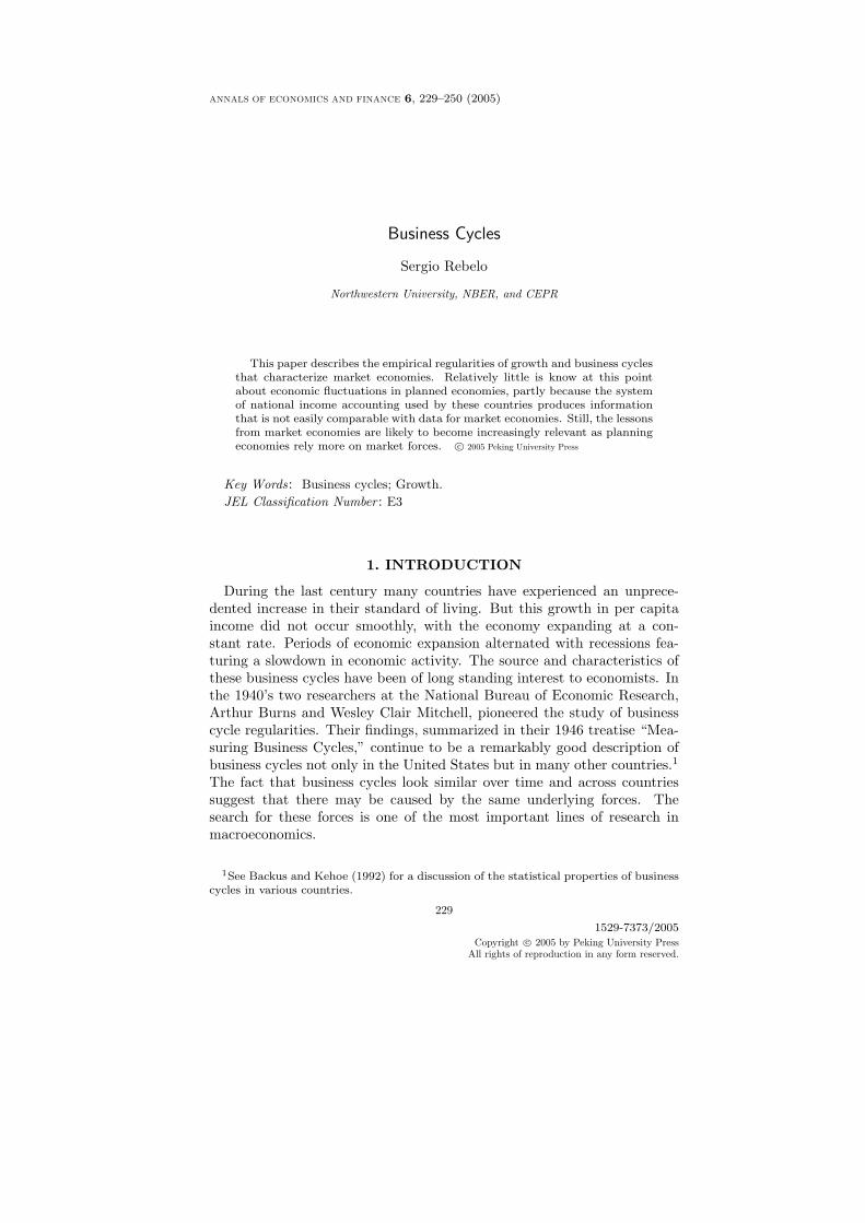
Kaldor (1957) first suggested that these variables might be constant inthe long run so this constancy is often referred to as the ‘Kaldor facts’.We will use a series of figures, extracted from Kongsamut, Rebelo andXie (2001) and King and Rebelo (1999), to depict the behavior of thesedifferent variables. Figure 1, which displays the U.S. real per capita GDP(in logarithms) for the period 1902 to 1999 shows that the U.S. growth ratecomputed over long periods of time (say, decades) has been surprisinglystable. The average annual growth rate of the U.S. economy during thisperiod is roughly 2 percent per year.

BUSINESS CYCLES 231

FIG. 1. U.S. Real GDP per capita, 1902-1999 (in logarithms)

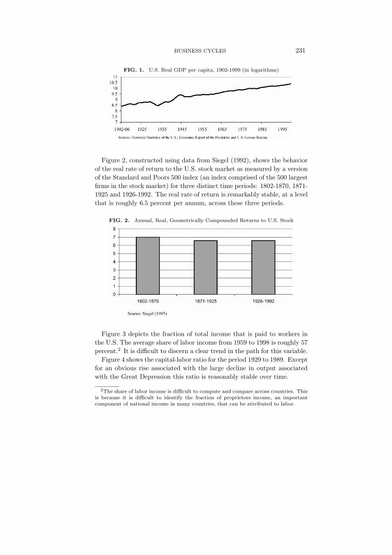
Figure 2, constructed using data from Siegel (1992), shows the behaviorof the real rate of return to the U.S. stock market as measured by a versionof the Standard and Poors 500 index (an index comprised of the 500 largestfirms in the stock market) for three distinct time periods: 1802-1870, 1871-1925 and 1926-1992. The real rate of return is remarkably stable, at a levelthat is roughly 6.5 percent per annum, across these three periods.

FIG. 2. Annual, Real, Geometrically Compounded Returns to U.S. Stock

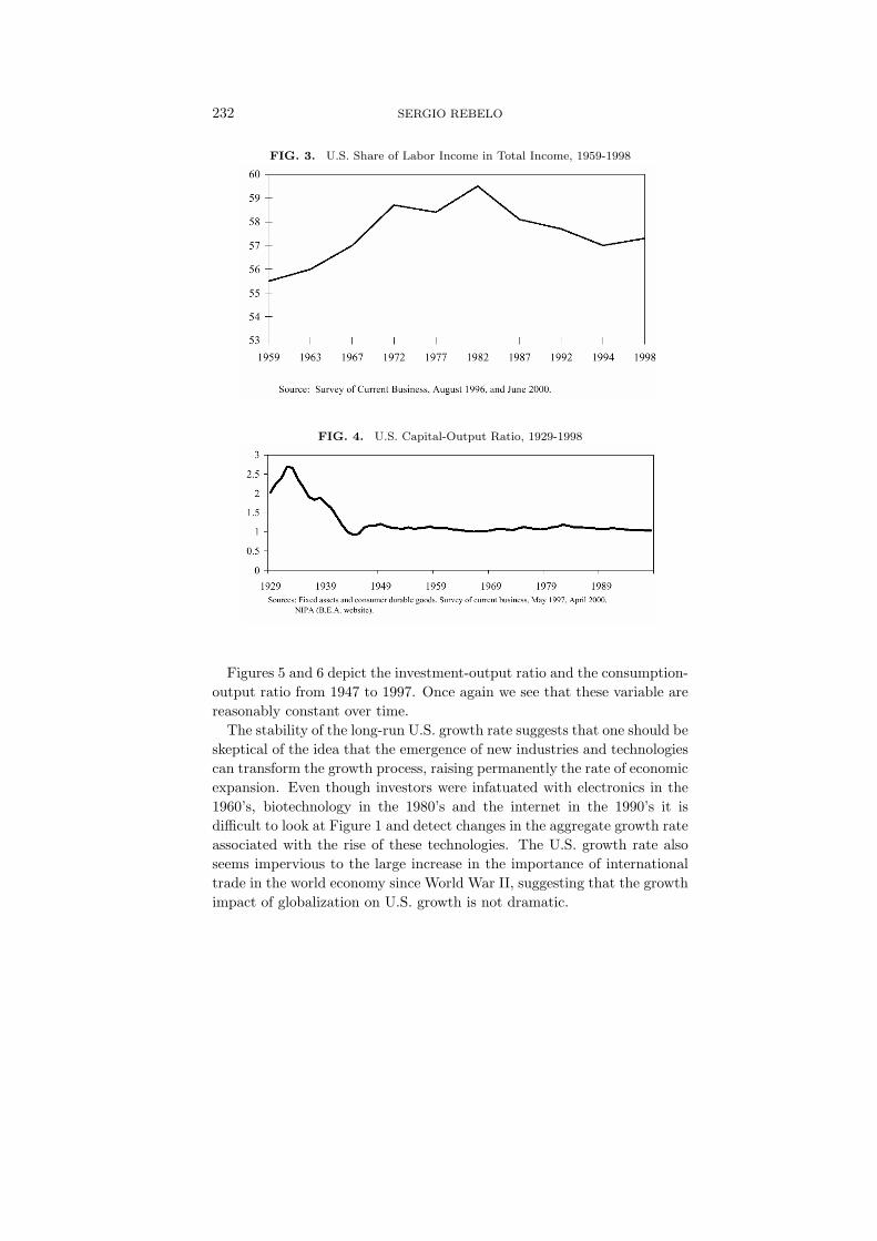
Figure 3 depicts the fraction of total income that is paid to workers inthe U.S. The average share of labor income from 1959 to 1998 is roughly 57percent.2 It is difficult to discern a clear trend in the path for this variable.

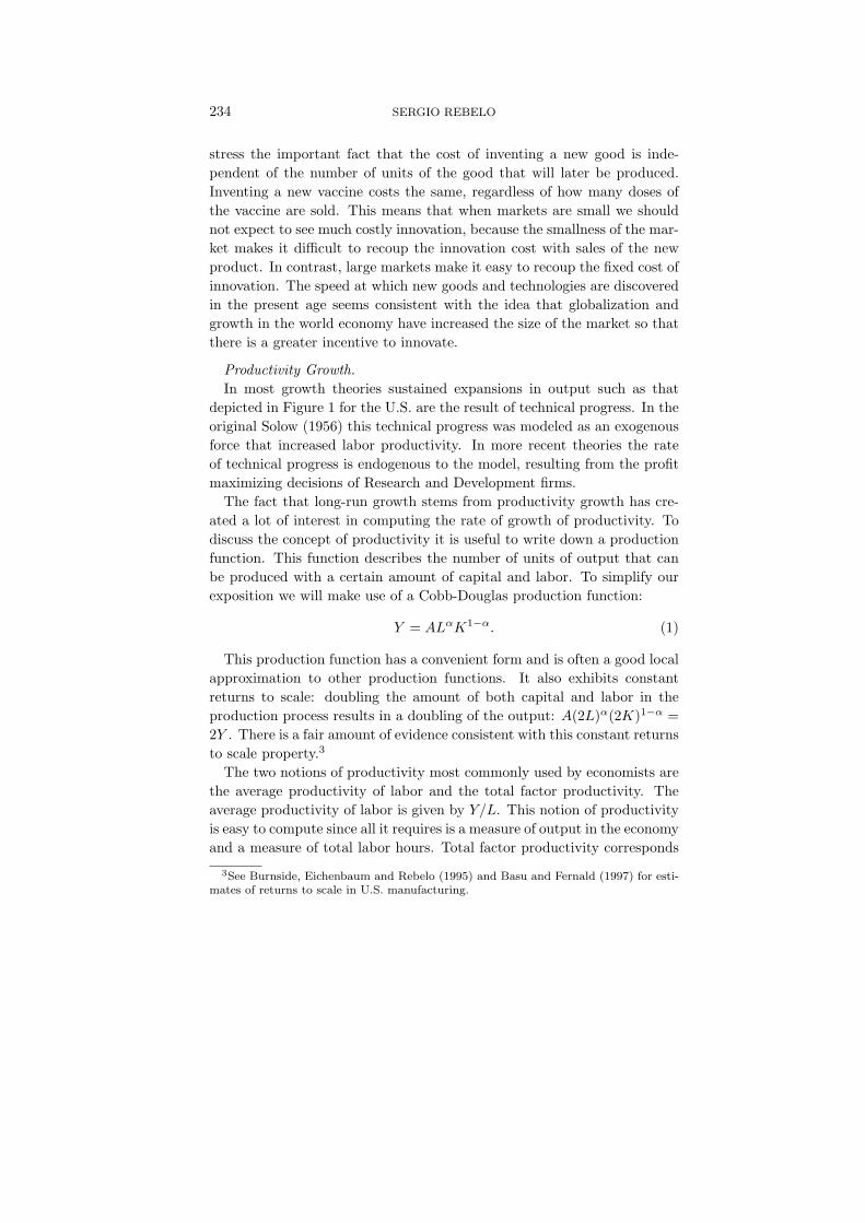
Figure 4 shows the capital-labor ratio for the period 1929 to 1989. Exceptfor an obvious rise associated with the large decline in output associatedwith the Great Depression this ratio is reasonably stable over time.

2The share of labor income is difficult to compute and compare across countries. Thisis because it is difficult to identify the fraction of proprietors income, an importantcomponent of national income in many countries, that can be attributed to labor.

232 SERGIO REBELO

FIG. 3. U.S. Share of Labor Income in Total Income, 1959-1998

FIG. 4. U.S. Capital-Output Ratio, 1929-1998

Figures 5 and 6 depict the investment-output ratio and the consumption-output ratio from 1947 to 1997. Once again we see that these variable arereasonably constant over time.

The stability of the long-run U.S. growth rate suggests that one should beskeptical of the idea that the emergence of new industries and technologiescan transform the growth process, raising permanently the rate of economicexpansion. Even though investors were infatuated with electronics in the1960’s, biotechnology in the 1980’s and the internet in the 1990’s it isdifficult to look at Figure 1 and detect changes in the aggregate growth rateassociated with the rise of these technologies. The U.S. growth rate alsoseems impervious to the large increase in the importance of internationaltrade in the world economy since World War II, suggesting that the growthimpact of globalization on U.S. growth is not dramatic.

BUSINESS CYCLES 233

FIG. 5.

FIG. 6.

It is important to caution that evidence in favor of the Kaldor factsis strongest in the U.S. economy during the period depicted in Figure 1.Data for other countries and longer run data for the U.S. is consistent withthe idea that there has been a slow but steady acceleration of the rate ofgrowth. This acceleration becomes obvious once we look beyond the lastcentury. As Lucas (1997) emphasized, the sustained growth suggested byFigure 1 is a recent phenomenon, that characterizes at best the last twohundred years. In pre-industrial times the level of income remained stableover long periods of time. This stability is reflected in the writings of theclassical economists–Smith, Ricardo and Malthus–who imagined a worldwhere sustained income growth was impossible.

Many theories of economic growth (e.g. Romer (1990), Grossman andHelpman (1991) and Aghion and Howitt (1992)) predict that the rate ofgrowth of the world economy should accelerate over time. These theories

234 SERGIO REBELO

stress the important fact that the cost of inventing a new good is inde-pendent of the number of units of the good that will later be produced.Inventing a new vaccine costs the same, regardless of how many doses ofthe vaccine are sold. This means that when markets are small we shouldnot expect to see much costly innovation, because the smallness of the mar-ket makes it difficult to recoup the innovation cost with sales of the newproduct. In contrast, large markets make it easy to recoup the fixed cost ofinnovation. The speed at which new goods and technologies are discoveredin the present age seems consistent with the idea that globalization andgrowth in the world economy have increased the size of the market so thatthere is a greater incentive to innovate.

Productivity Growth.In most growth theories sustained expansions in output such as that

depicted in Figure 1 for the U.S. are the result of technical progress. In theoriginal Solow (1956) this technical progress was modeled as an exogenousforce that increased labor productivity. In more recent theories the rateof technical progress is endogenous to the model, resulting from the profitmaximizing decisions of Research and Development firms.

The fact that long-run growth stems from productivity growth has cre-ated a lot of interest in computing the rate of growth of productivity. Todiscuss the concept of productivity it is useful to write down a productionfunction. This function describes the number of units of output that canbe produced with a certain amount of capital and labor. To simplify ourexposition we will make use of a Cobb-Douglas production function:

Y = ALαK1−α. (1)

This production function has a convenient form and is often a good localapproximation to other production functions. It also exhibits constantreturns to scale: doubling the amount of both capital and labor in theproduction process results in a doubling of the output: A(2L)α(2K)1−α =2Y . There is a fair amount of evidence consistent with this constant returnsto scale property.3

The two notions of productivity most commonly used by economists arethe average productivity of labor and the total factor productivity. Theaverage productivity of labor is given by Y/L. This notion of productivityis easy to compute since all it requires is a measure of output in the economyand a measure of total labor hours. Total factor productivity corresponds

3See Burnside, Eichenbaum and Rebelo (1995) and Basu and Fernald (1997) for esti-mates of returns to scale in U.S. manufacturing.

BUSINESS CYCLES 235

to the variable A in equation (1). Computing A is harder since it requiresan estimate of the stock of capital and of the elasticity α. The stock ofcapital is usually estimated with the “perpetual inventory method”. Thisrelies on the following equation:4

Kt+1 = It + (1− δ)Kt (2)

where It represents investment in physical capital, Kt is the capital stockat date t and δ is the rate of depreciation. Given an estimate of the initialcapital stock at some point in the past, we can use a time series for invest-ment, together with equation (1) to generate a time series for the stock ofcapital. The value of α is usually computed by using the fact that whenfactor markets are competitive α coincides with the share of labor incomein the economy.

Once we obtain a time series for the stock of capital and a value for α wecan compute total factor productivity. Macroeconomists are usually notinterested in the level of total factor productivity but on its growth rate.It is this growth rate that drives the long run rate of expansion in manymodels. The growth rate of A can be computed as:

gA = gY − αgL − (1− α)gK

where we used the notation gx to denote the continuously compounded rateof growth (ln(xt+1/xt)) of variable x. We will later discuss the behavior ofthese two notions of productivity over the business cycle.

The Kuznets Facts.In countries such as the U.S., long-run growth in income has been rel-

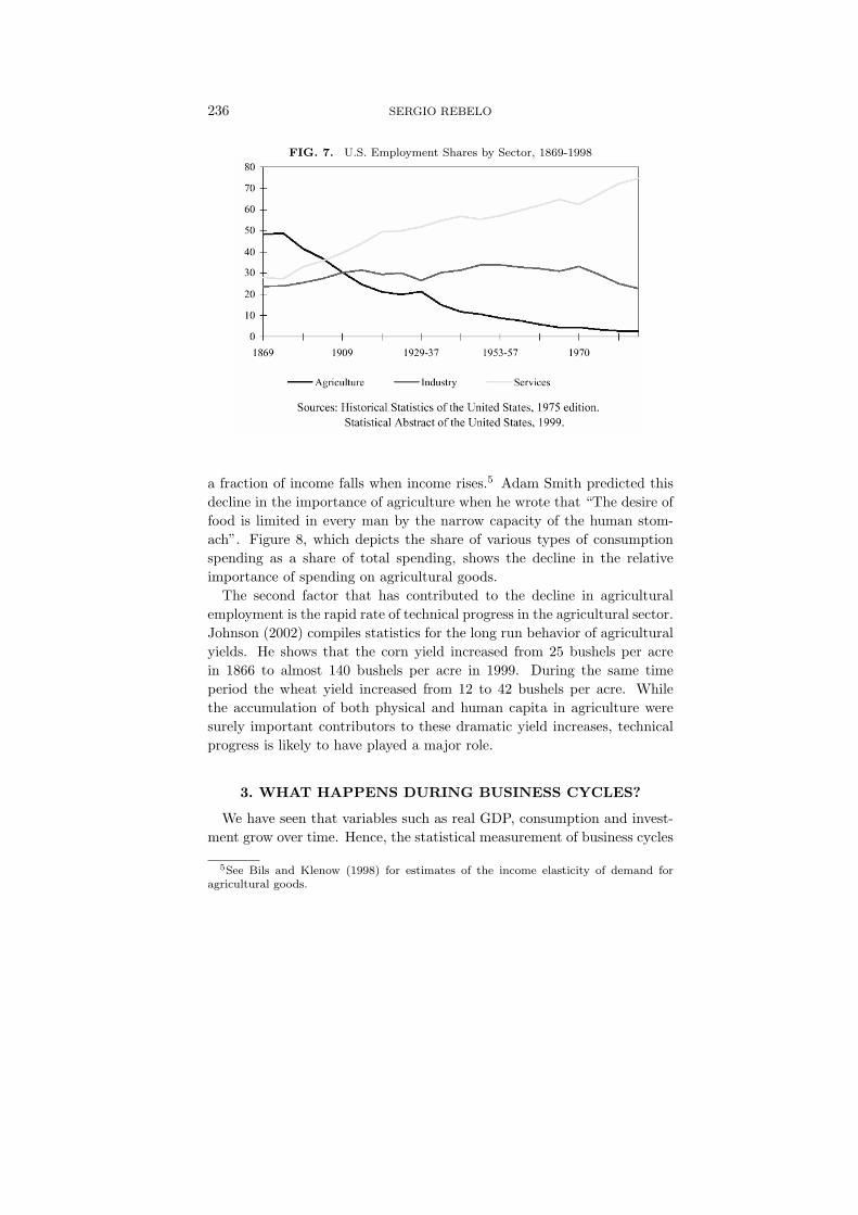
atively smooth at the aggregate level for at least one century. However,during this period of time, the sectoral composition of the economy haschanged dramatically. Agriculture, which accounted for almost 50 percentof employment in 1869 was reduced to less than 2 percent of employment by1998. Figure 7 shows the enormous sectoral reallocation of labor that hastaken place in the U.S. since 1869, with a dramatic decline in employmentin agriculture and a rise in service employment.

This decline in the importance of agriculture is likely to have been theresult of two factors. First, the income elasticity of the demand for agricul-tural goods is less than one, so the percentage of income spent on food as

4In practice the perpetual inventory method does not assume that the rate of depre-ciation, δ, is constant.

236 SERGIO REBELO

FIG. 7. U.S. Employment Shares by Sector, 1869-1998

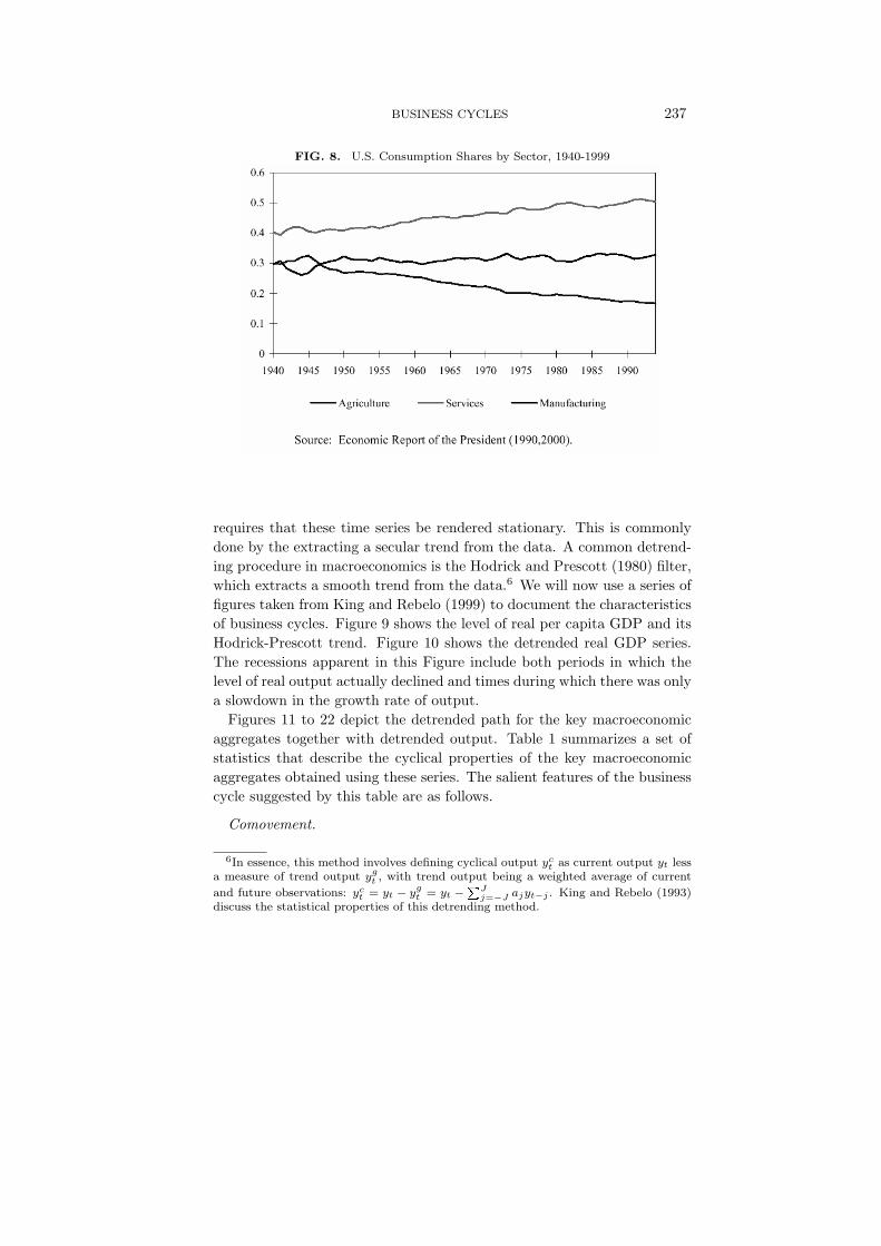
a fraction of income falls when income rises.5 Adam Smith predicted thisdecline in the importance of agriculture when he wrote that “The desire offood is limited in every man by the narrow capacity of the human stom-ach”. Figure 8, which depicts the share of various types of consumptionspending as a share of total spending, shows the decline in the relativeimportance of spending on agricultural goods.

The second factor that has contributed to the decline in agriculturalemployment is the rapid rate of technical progress in the agricultural sector.Johnson (2002) compiles statistics for the long run behavior of agriculturalyields. He shows that the corn yield increased from 25 bushels per acrein 1866 to almost 140 bushels per acre in 1999. During the same timeperiod the wheat yield increased from 12 to 42 bushels per acre. Whilethe accumulation of both physical and human capita in agriculture weresurely important contributors to these dramatic yield increases, technicalprogress is likely to have played a major role.

3. WHAT HAPPENS DURING BUSINESS CYCLES?

We have seen that variables such as real GDP, consumption and invest-ment grow over time. Hence, the statistical measurement of business cycles

5See Bils and Klenow (1998) for estimates of the income elasticity of demand foragricultural goods.

BUSINESS CYCLES 237

FIG. 8. U.S. Consumption Shares by Sector, 1940-1999

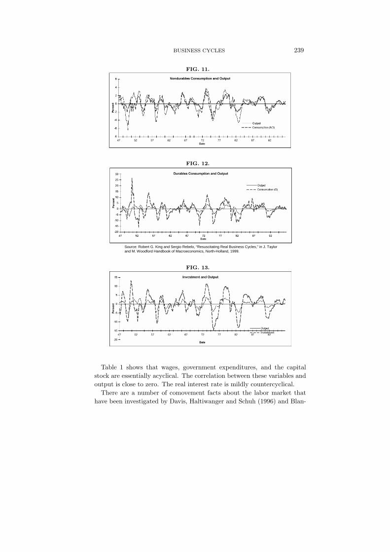
requires that these time series be rendered stationary. This is commonlydone by the extracting a secular trend from the data. A common detrend-ing procedure in macroeconomics is the Hodrick and Prescott (1980) filter,which extracts a smooth trend from the data.6 We will now use a series offigures taken from King and Rebelo (1999) to document the characteristicsof business cycles. Figure 9 shows the level of real per capita GDP and itsHodrick-Prescott trend. Figure 10 shows the detrended real GDP series.The recessions apparent in this Figure include both periods in which thelevel of real output actually declined and times during which there was onlya slowdown in the growth rate of output.

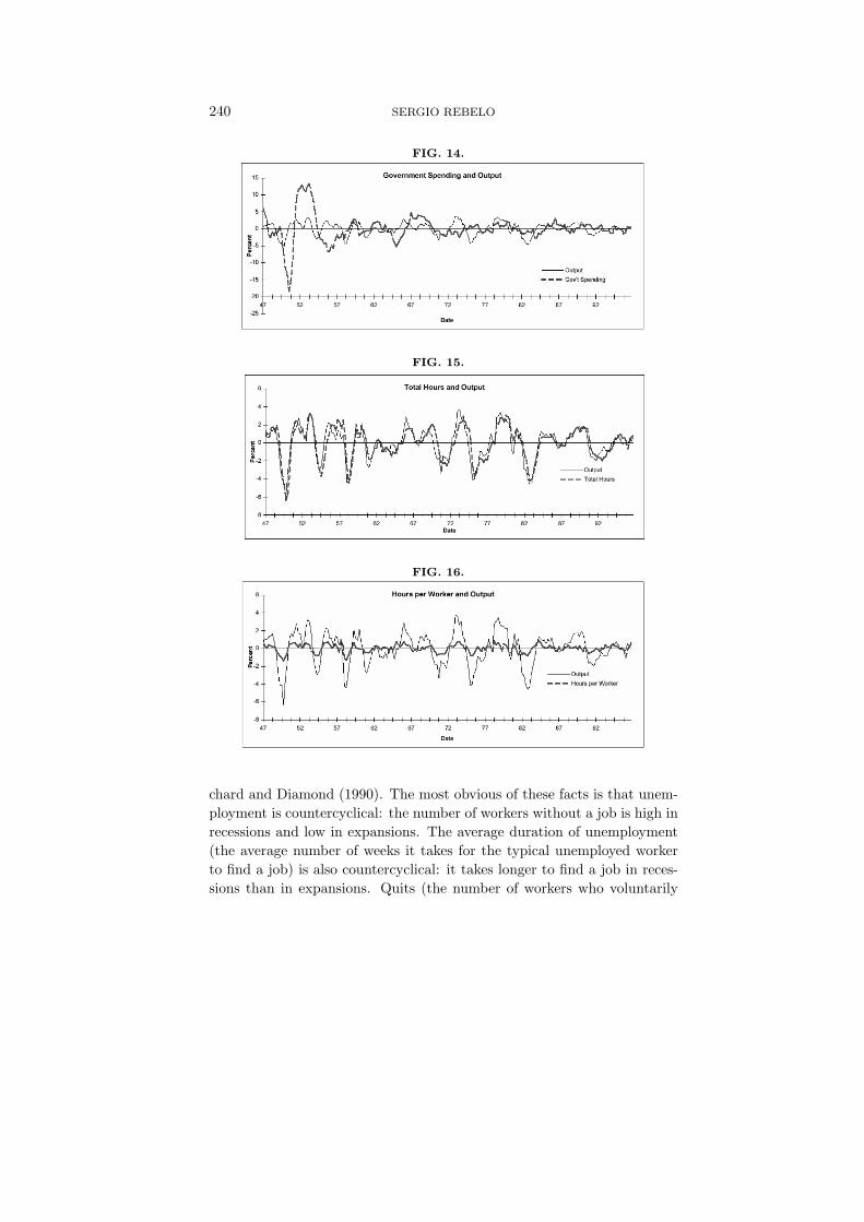
Figures 11 to 22 depict the detrended path for the key macroeconomicaggregates together with detrended output. Table 1 summarizes a set ofstatistics that describe the cyclical properties of the key macroeconomicaggregates obtained using these series. The salient features of the businesscycle suggested by this table are as follows.

Comovement.

6In essence, this method involves defining cyclical output yct as current output yt less

a measure of trend output ygt , with trend output being a weighted average of current

and future observations: yct = yt − yg

t = yt −PJ

j=−J ajyt−j . King and Rebelo (1993)discuss the statistical properties of this detrending method.

238 SERGIO REBELO

FIG. 9.

Output and its Trend

7.2

7.4

7.6

7.8

8

8.2

8.4

8.6

8.8

47 52 57 62 67 72 77 82 87 92

Date

Lo

ga

rith

m

Output

Trend

Source: Robert G. King and Sergio Rebelo, “Resuscitating Real Business Cycles,” in J. Taylor and M. Woodford Handbook of Macroeconomcs, North-Holland, 1999.

FIG. 10.

Detrended Real GDP

-8

-6

-4

-2

0

2

4

6

47 52 57 62 67 72 77 82 87 92

Date

Pe

rce

nt

Korean War

Suez Crisis Vietnam War

Second Oil Shock

Reagan Expansion

Gulf Crisis

Volcker Restraint

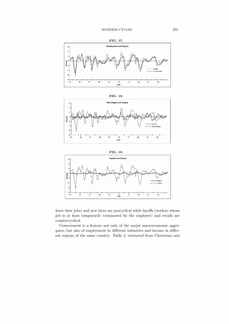
Most macroeconomic aggregates are procyclical, that is, they are pos-itively correlated with output.7 This means that an expansion is like aneconomic crescendo: output, consumption, investment, total hours workedin the economy, average labor productivity and total factor productivityall tend to rise simultaneously. Table 1 shows that high degree of corre-lation between these variables and aggregate output (ranging from .88 forconsumption and labor to .55 for labor productivity). This high degree ofcoherence can also be gleaned from Figures 11 to 21.

7The trade balance, which is countercyclical, is an important exception.

BUSINESS CYCLES 239

FIG. 11.

FIG. 12.

Source: Robert G. King and Sergio Rebelo, “Resuscitating Real Business Cycles,” in J. Taylor and M. Woodford Handbook of Macroeconomics, North-Holland, 1999.

FIG. 13.

Table 1 shows that wages, government expenditures, and the capitalstock are essentially acyclical. The correlation between these variables andoutput is close to zero. The real interest rate is mildly countercyclical.

There are a number of comovement facts about the labor market thathave been investigated by Davis, Haltiwanger and Schuh (1996) and Blan-

240 SERGIO REBELO

FIG. 14.

FIG. 15.

FIG. 16.

chard and Diamond (1990). The most obvious of these facts is that unem-ployment is countercyclical: the number of workers without a job is high inrecessions and low in expansions. The average duration of unemployment(the average number of weeks it takes for the typical unemployed workerto find a job) is also countercyclical: it takes longer to find a job in reces-sions than in expansions. Quits (the number of workers who voluntarily

BUSINESS CYCLES 241

FIG. 17.

FIG. 18.

FIG. 19.

leave their jobs) and new hires are procyclical while layoffs (workers whosejob is at least temporarily terminated by the employer) and recalls arecountercyclical.

Comovement is a feature not only of the major macroeconomic aggre-gates, but also of employment in different industries and income in differ-ent regions of the same country. Table 2, extracted from Christiano and

242 SERGIO REBELO

FIG. 20.

FIG. 21.

-2

-1.5

-1

-0.5

0

0.5

1

1.5

2

1947 1950 1953 1956 1959 1962 1965 1968 1971 1974 1977 1980 1983 1986 1989 1992

output trade balance

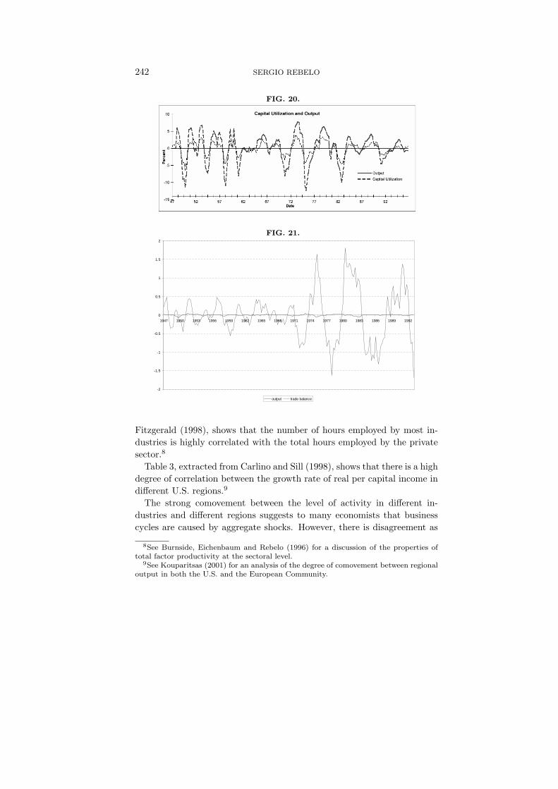
Fitzgerald (1998), shows that the number of hours employed by most in-dustries is highly correlated with the total hours employed by the privatesector.8

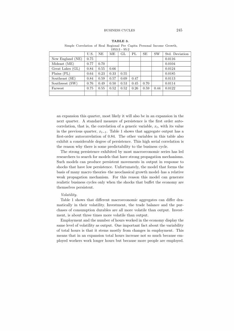
Table 3, extracted from Carlino and Sill (1998), shows that there is a highdegree of correlation between the growth rate of real per capital income indifferent U.S. regions.9

The strong comovement between the level of activity in different in-dustries and different regions suggests to many economists that businesscycles are caused by aggregate shocks. However, there is disagreement as

8See Burnside, Eichenbaum and Rebelo (1996) for a discussion of the properties oftotal factor productivity at the sectoral level.

9See Kouparitsas (2001) for an analysis of the degree of comovement between regionaloutput in both the U.S. and the European Community.

BUSINESS CYCLES 243

FIG. 22.

-25

-20

-15

-10

-5

0

5

10

15

20

1889 1899 1909 1919 1929 1939 1949 1959 1969 1979 1989

Growth Rate of Per Capita Real GDP

TABLE 1.

Business Cycle Statistics for the U.S. Economy

Standard Relative First Contemporaneous

Deviation Standard Order Correlation

Deviation Auto with

-correlation Output

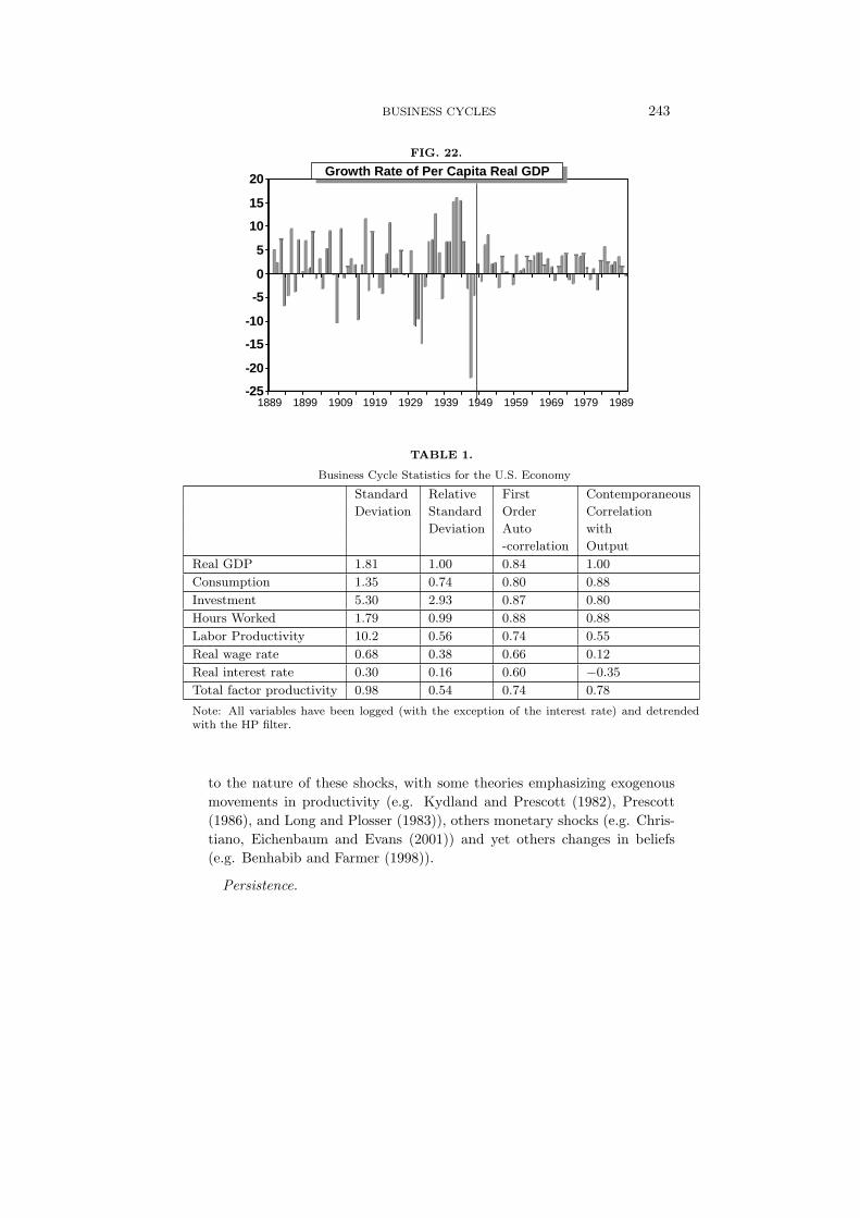
Real GDP 1.81 1.00 0.84 1.00

Consumption 1.35 0.74 0.80 0.88

Investment 5.30 2.93 0.87 0.80

Hours Worked 1.79 0.99 0.88 0.88

Labor Productivity 10.2 0.56 0.74 0.55

Real wage rate 0.68 0.38 0.66 0.12

Real interest rate 0.30 0.16 0.60 −0.35

Total factor productivity 0.98 0.54 0.74 0.78

Note: All variables have been logged (with the exception of the interest rate) and detrendedwith the HP filter.

to the nature of these shocks, with some theories emphasizing exogenousmovements in productivity (e.g. Kydland and Prescott (1982), Prescott(1986), and Long and Plosser (1983)), others monetary shocks (e.g. Chris-tiano, Eichenbaum and Evans (2001)) and yet others changes in beliefs(e.g. Benhabib and Farmer (1998)).

Persistence.

244 SERGIO REBELO

TABLE 2.

Properties of the business cycle components of hours worked

Variable Relative Relative Business cycle

number Hours worked variable magnitude volatility comovement

1 Total private 1.00 1.00 .00

2 Goods producing industries .33 2.91 .99

3 Mining .03 5.48 .38

4 Construction .17 6.75 .88

5 Manufacturing .80 3.92 .97

6 Durable goods .58 6.90 .97

7 Lurnber and wood products .06 10.18 .89

8 Furnture and fixtures .04 8.14 .94

9 Store, clay, and glass products .05 4.99 .95

10 Primary metal industries .09 9.89 .88

11 Fabricated metal products .13 7.21 .98

12 Machinery, except electrical .19 11.10 .93

13 Electrical and electronic equipment .15 8.75 .88

14 Transportation equipment .17 7.83 .89

15 Instruments and related products .09 5.03 .78

16 Miscellaneous manufacturing .04 3.23 .90

17 Nondurable goods .42 1.39 .91

18 Food and kindred products .21 .18 .50

19 Tobacco manufactures .01 1.83 .08

20 Textile mill products .11 3.92 .78

21 Apparel and other textile products .15 2.64 .85

22 Paper and allied products .09 1.97 .85

23 Printing and publishing .16 .91 .90

24 Chemicals and allied products .13 1.01 .80

25 Petroleum and coal products .02 2.02 .16

26 Rubber and misc. plastics products .09 7.82 .89

27 Leather and leather products .03 2.71 .64

28 Rubber and misc. plastics products .02 2.02 .18

29 Transportation and public utilities .10 .87 .95

30 Wholesale trade .10 .85 .87

31 Retail trade .31 .38 .87

32 Finance, insurance, and real estate .10 .35 .48

33 Services .38 .19 .49

Another notable feature of the business cycle is that recessions and ex-pansions tend to be protracted. The economy does not alternate quicklybetween periods of growth and period of contraction. If an economy is in

BUSINESS CYCLES 245

TABLE 3.

Simple Correlation of Real Regional Per Capita Personal Income Growth,1953:3 - 95:2

U.S. NE ME GL PL SE SW Std. Deviation

New England (NE) 0.75 0.0116

Mideast (ME) 0.77 0.70 0.0104

Great Lakes (GL) 0.84 0.55 0.66 0.0124

Plains (PL) 0.64 0.23 0.33 0.55 0.0185

Southeast (SE) 0.84 0.59 0.57 0.69 0.47 0.0113

Southwest (SW) 0.76 0.49 0.50 0.53 0.45 0.70 0.0114

Farwest 0.75 0.55 0.52 0.52 0.26 0.59 0.44 0.0122

an expansion this quarter, most likely it will also be in an expansion in thenext quarter. A standard measure of persistence is the first order auto-correlation, that is, the correlation of a generic variable, xt, with its valuein the previous quarter, xt−1. Table 1 shows that aggregate output has afirst-order autocorrelation of 0.84. The other variables in this table alsoexhibit a considerable degree of persistence. This high serial correlation isthe reason why there is some predictability to the business cycle.

The strong persistence exhibited by most macroeconomic series has ledresearchers to search for models that have strong propagation mechanisms.Such models can produce persistent movements in output in response toshocks that have low persistence. Unfortunately, the model that forms thebasis of many macro theories–the neoclassical growth model–has a relativeweak propagation mechanism. For this reason this model can generaterealistic business cycles only when the shocks that buffet the economy arethemselves persistent.

Volatility.Table 1 shows that different macroeconomic aggregates can differ dra-

matically in their volatility. Investment, the trade balance and the pur-chases of consumption durables are all more volatile than output. Invest-ment, is about three times more volatile than output.

Employment and the number of hours worked in the economy display thesame level of volatility as output. One important fact about the variabilityof total hours is that it stems mostly from changes in employment. Thismeans that in an expansion total hours increase not so much because em-ployed workers work longer hours but because more people are employed.

246 SERGIO REBELO

Similarly, in recessions total hours worked decline mostly because the levelof employment declines.

Among the variables that are less volatile than output the most impor-tant are the consumption of non-durable goods, the average hours workedand the real wage.

The capital stock has much lower volatility than output, displaying verylittle cyclical variation (see Figure 19).

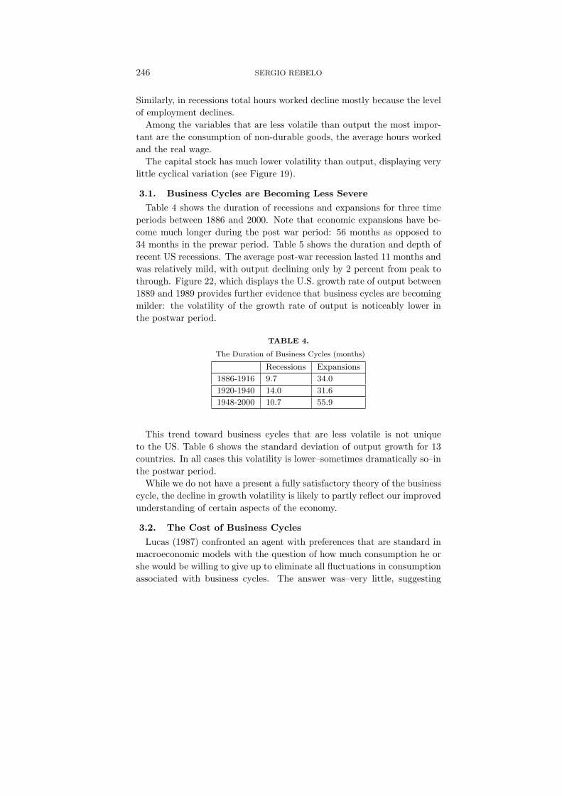
3.1. Business Cycles are Becoming Less Severe

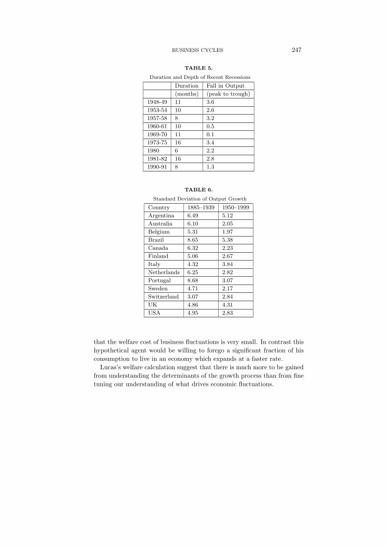
Table 4 shows the duration of recessions and expansions for three timeperiods between 1886 and 2000. Note that economic expansions have be-come much longer during the post war period: 56 months as opposed to34 months in the prewar period. Table 5 shows the duration and depth ofrecent US recessions. The average post-war recession lasted 11 months andwas relatively mild, with output declining only by 2 percent from peak tothrough. Figure 22, which displays the U.S. growth rate of output between1889 and 1989 provides further evidence that business cycles are becomingmilder: the volatility of the growth rate of output is noticeably lower inthe postwar period.

TABLE 4.

The Duration of Business Cycles (months)

Recessions Expansions

1886-1916 9.7 34.0

1920-1940 14.0 31.6

1948-2000 10.7 55.9

This trend toward business cycles that are less volatile is not uniqueto the US. Table 6 shows the standard deviation of output growth for 13countries. In all cases this volatility is lower–sometimes dramatically so–inthe postwar period.

While we do not have a present a fully satisfactory theory of the businesscycle, the decline in growth volatility is likely to partly reflect our improvedunderstanding of certain aspects of the economy.

3.2. The Cost of Business Cycles

Lucas (1987) confronted an agent with preferences that are standard inmacroeconomic models with the question of how much consumption he orshe would be willing to give up to eliminate all fluctuations in consumptionassociated with business cycles. The answer was–very little, suggesting

BUSINESS CYCLES 247

TABLE 5.

Duration and Depth of Recent Recessions

Duration Fall in Output

(months) (peak to trough)

1948-49 11 3.6

1953-54 10 2.6

1957-58 8 3.2

1960-61 10 0.5

1969-70 11 0.1

1973-75 16 3.4

1980 6 2.2

1981-82 16 2.8

1990-91 8 1.3

TABLE 6.

Standard Deviation of Output Growth

Country 1885–1939 1950–1999

Argentina 6.49 5.12

Australia 6.10 2.05

Belgium 5.31 1.97

Brazil 8.65 5.38

Canada 6.32 2.23

Finland 5.06 2.67

Italy 4.32 3.84

Netherlands 6.25 2.82

Portugal 8.68 3.07

Sweden 4.71 2.17

Switzerland 3.07 2.84

UK 4.86 4.31

USA 4.95 2.83

that the welfare cost of business fluctuations is very small. In contrast thishypothetical agent would be willing to forego a significant fraction of hisconsumption to live in an economy which expands at a faster rate.

Lucas’s welfare calculation suggest that there is much more to be gainedfrom understanding the determinants of the growth process than from finetuning our understanding of what drives economic fluctuations.

248 SERGIO REBELO

4. BUSINESS CYCLE FACTS AND MACROECONOMICTHEORIES

The facts that we discussed in this paper have greatly influenced thedevelopment of macroeconomic theories. The smoothness of non-durableconsumption has led macroeconomics to model consumers as having pref-erences that assign higher utility to smooth consumption paths. The highvolatility of investment underlies Keynes’s notion that investmentor sen-timent may be an important influence on investment behavior. The lowcyclical volatility of capital is often taken to imply that one can safelyabstract from movements in capital in constructing a theory of economicfluctuations. But while the stock of capital is relatively immutable at cycli-cal frequencies, the intensity with which the capital is utilized displays largevariation over the business cycle. This has motivated the development ofmodels that emphasize capital utilization.10 The high correlation betweenhours worked and aggregate output has led some economists to believe thatunderstanding the labor market is key to understanding business fluctua-tions. Finally, the relatively small variability of real wages and the lackof a close correspondence of wages with aggregate output, has led someeconomists to conclude that the wage rate is not an important allocativesignal in the business cycle.

REFERENCESAghion, P. and P. Howitt, 1992. A model of growth through creative destruction.Econometrica 60, 323-351.

Backus, D. and P. Kehoe, 1992. International evidence on the historical properties ofbusiness cycles. American Economic Review 82, 864-88.

Basu, S. and J. G. Fernald, 1997. Returns to scale in U.S. production: Estimates andimplications. Journal of Political Economy 105, 249-283.

Benhabib, J. and R. Farmer, 1998. Indeterminacy and sunspots in macroeconomics.Handbook of Macroeconomics. North-Holland.

Bils, M. and J. O. Cho, 1994. Cyclical factor utilization. Journal of Monetary Eco-nomics 33, 319-354.

Bils, M. and P. Klenow, 1998. Using consumer theory to test competing businesscycle models. Journal of Political Economy 106, 233-261.

Blanchard, O. J. and P. Diamond, 1990. The cyclical behavior of the gross flows ofU.S. workers. Brookings Papers on Economic Activity. 85-155.

Burns, A. F. and W. C. Mitchell, 1946. Measuring business cycles. National Bureauof Economic Research. New York.

10See, for example, Greenwood, Hercowitz, and Huffman (1988), Bils and Cho (1994),Burnside and Eichenbaum (1996), and Burnside, Eichenbaum, and Rebelo (1995).

BUSINESS CYCLES 249

Burnside, C. and M. Eichenbaum, 1996. Factor hoarding and the propagation ofbusiness cycle shocks. American Economic Review 86, 1154-1174.

Burnside, C., M. Eichenbaum, and S. Rebelo, 1995. Capital utilization and returnsto scale. NBER Macroeconomics Annual 1995. 67-110, MIT Press, Cambridge, MA.

Burnside, C., M. Eichenbaum, and S. Rebelo, 1996. Sectoral Solow residuals. Euro-pean Economic Review 40, 861-869.

Carlino, G. and K. Sill, 1998. The cyclical behavior of regional per capita income inthe post war period. Working Paper. Federal Reserve Bank of Philadelphia.

Christiano, L. and T. J. Fitzgerald, 1998. The business cycle: It’s still a puzzle.Economic Perspectives.

Christiano, L., M. Eichenbaum, and C. Evans, 2002. Nominal rigidities and the dy-namic effects of a shock to monetary policy. Mimeo.

Davis, S., J. Haltiwanger, and S. Schuh, 1996. Job Creation and Destruction. MITPress.

Greenwood, J., Z. Hercowitz, and G. Huffman, 1988. Investment, capacity utilization,and the business cycle. American Economic Review 78, 402-417.

Grossman, G. and E. Helpman, 1991. Quality ladders in the theory of growth. Reviewof Economic Studies 58, 43-61.

Hodrick, R. and E. Prescott, 1980. Post-war business cycles: An empirical investiga-tion. Working Paper. Carnegie-Mellon University.

Johnson, G., 2002. The declining importance of natural resources: Lessons from agri-cultural land. Resource and Energy Economics 24, 157-171.

Kaldor, N., 1957. A model of economic growth. Economic Journal 67, 591-624.

King, R. and S. Rebelo, 1993. Low frequency filtering and real business cycles. Journalof Economic Dynamics and Control 17, 207-231.

King, R. and S. Rebelo, 1999. Resuscitating real business cycles. In: J. Taylor andM. Woodford Handbook of Macroeconomics. North-Holland.

Kongsamut, P., S. Rebelo, and D. Xie, 2001. Beyond balanced growth. Review ofEconomic Studies 68, 869-882.

Kouparitsas, M., 2001. Is the United States an optimum currency area? An empiricalanalysis of regional business cycles. Mimeo. Federal Reserve Bank of Chicago.

Kydland, F. and E. Prescott, 1982. Time to build and aggregate fluctuations. Econo-metrica 50, 1345-1370.

Long, J. and C. Plosser, 1983. Real business cycles. Journal of Political Economy 91,1345-1370.

Lucas, R. E., 1987. Models of Business Cycles. Basil Blackwell.

Lucas, R., 1997. The Industrial revolution: Past and future. The Kuznets Lectures.University of Chicago.

Miles, D. and A. Scott, 2001. Macroeconomics: Understanding the Wealth of Nations.Wiley.

Prescott, E., 1986. Theory ahead of business-cycle measurement. Federal ReserveBank of Minneapolis Quarterly Review 10, 9-22.

Romer, C., 1994. Remeasuring business cycles. Journal of Economic History 54,573-609.

Romer, P., 1990. Endogenous technical change. Journal of Political Economy 98,S71-S102.

250 SERGIO REBELO

Siegel, J., 1992. The real interest rate from 1800-1990: A study of the U.S. and theU.K. Journal of Monetary Economics 29, 227-252.

Solow, R., 1956. A contribution to the theory of economic growth. Quarterly Journalof Economics 70, 65-94.