Burning Characteristics of Individual Douglas-Fir Trees inthe Wildland/Urban Interface

by

Elisa Schulz Baker

A Thesis

Submitted to the Faculty

of the

WORCESTER POLYTECHNIC INSTITUTE

In partial fulfillment of the requirements for the

Degree of Master of Science

in

Fire Protection Engineering

by

Elisa Schulz BakerJune 2011

APPROVED:

Professor Albert J. Simeoni, PhD., Major Advisor

Alexander Maranghides, Reader

Professor Kathy A. Notarianni, PhD., Head of Department

Abstract

The Wildland/Urban Interface, in which homes are intermingled with forested ar-

eas, presents unique challenges to fire protection and fire prediction, owing to the

different fuel loads, conditions, and terrain. Computer models that predict fire

spread through such an area require data for multiple scales, from crown fire spread

to the heat release rates and ignition conditions for individual trees, as well as an

understanding of fire behavior and spread. This discussion investigates a means

by which fire behavior for Douglas-fir trees can be determined from quantifiable

characteristics, such as height and moisture content. Mass, flame height, peak heat

release rate, and total energy can be estimated from these simple measurements.

A time scale of 60 seconds, combined with a peak heat release rate estimated from

tree size characteristics, provides an approximation of total energy that is within

11% of measured values. Pre-heating of trees with a low (2.5 kW/m2) radiant heat

flux did not have a noticeable impact on the resulting heat release rate. In addition,

fire spread between trees was highly dependent on the presence of ambient wind;

in the absence of wind or wind-borne embers, the trees were very resistant to igni-

tion even when in close proximity (3 spacing). With the addition of wind, the fire

would spread, although the heat release rates were dramatically reduced for trees of

sufficiently high moisture content (< 70%).

Acknowledgements

I would like to thank the Fire Protection Department of WPI, who in 2002

approved an internship with NIST, and then in 2003 extended it for a year in order

to allow me to continue with the fire tests and turn the experience into a thesis.

Certainly many thanks to Kathy Notarianni, and Dave Lucht are owed. Also to

Alex Maranghedes for allowing me to assist with the tree burning tests, and serving

as reader for this thesis. Thanks are due to John Woycheese, my initial advisor who

had many great suggestions and editorial assistance, Professor Simeoni for stepping

in to take over, and Kathy again for helping me to finish up, at long last.

Also many thanks to friends and family who have never ceased cheering me on.

i

Contents

1 Introduction 1

1.1 Chapter Descriptions . . . . . . . . . . . . . . . . . . . . . . . . . . . 2

1.1.1 Tree Size Variation and Scaling of Data . . . . . . . . . . . . . 3

1.1.2 Exposure to Radiant Heat Before Ignition . . . . . . . . . . . 3

1.1.3 Fire Spread Amongst Closely Grouped Trees . . . . . . . . . . 4

2 Background Information 5

2.1 Previous Work Done . . . . . . . . . . . . . . . . . . . . . . . . . . . 5

2.1.1 Heat Release Rate Studies . . . . . . . . . . . . . . . . . . . . 5

2.1.2 Flammability of Landscaping Plants . . . . . . . . . . . . . . 6

2.1.3 Radiant Pre-Heating . . . . . . . . . . . . . . . . . . . . . . . 7

2.2 Review of the Current State of Fire Models . . . . . . . . . . . . . . . 8

3 Tree Size Variation and Scaling of Data 11

3.1 Methodology . . . . . . . . . . . . . . . . . . . . . . . . . . . . . . . 11

3.1.1 Instrumentation . . . . . . . . . . . . . . . . . . . . . . . . . . 12

3.1.2 Trees . . . . . . . . . . . . . . . . . . . . . . . . . . . . . . . . 14

3.1.3 Test Procedure . . . . . . . . . . . . . . . . . . . . . . . . . . 17

3.2 Results and Analysis . . . . . . . . . . . . . . . . . . . . . . . . . . . 18

3.2.1 Moisture Content . . . . . . . . . . . . . . . . . . . . . . . . . 18

ii

3.2.2 Mass loss . . . . . . . . . . . . . . . . . . . . . . . . . . . . . 23

3.2.3 HRR . . . . . . . . . . . . . . . . . . . . . . . . . . . . . . . . 26

3.2.4 Tree Mass as a Function of Height and Leaf Area . . . . . . . 30

3.2.5 Imaging (Flame Characteristics) . . . . . . . . . . . . . . . . . 34

3.2.6 Flame Temperatures . . . . . . . . . . . . . . . . . . . . . . . 40

3.2.7 Heat Flux . . . . . . . . . . . . . . . . . . . . . . . . . . . . . 43

3.2.8 Comparison Across Species . . . . . . . . . . . . . . . . . . . . 47

4 Exposure to Radiant Heat Before Ignition 50

4.1 Methodology . . . . . . . . . . . . . . . . . . . . . . . . . . . . . . . 51

4.1.1 Instrumentation . . . . . . . . . . . . . . . . . . . . . . . . . . 51

4.1.2 Procedure . . . . . . . . . . . . . . . . . . . . . . . . . . . . . 57

4.2 Results and Analysis . . . . . . . . . . . . . . . . . . . . . . . . . . . 63

4.2.1 Moisture Content . . . . . . . . . . . . . . . . . . . . . . . . . 64

4.2.2 Mass Loss . . . . . . . . . . . . . . . . . . . . . . . . . . . . . 68

4.2.3 Heat Release Rates . . . . . . . . . . . . . . . . . . . . . . . . 69

4.2.4 Leaf Area . . . . . . . . . . . . . . . . . . . . . . . . . . . . . 72

5 Fire Spread Amongst Closely Grouped Trees 76

5.1 Procedure . . . . . . . . . . . . . . . . . . . . . . . . . . . . . . . . . 77

5.2 Results and Analysis . . . . . . . . . . . . . . . . . . . . . . . . . . . 87

6 Uncertainty 90

6.1 Thermocouples . . . . . . . . . . . . . . . . . . . . . . . . . . . . . . 91

6.2 Heat Flux Gauges . . . . . . . . . . . . . . . . . . . . . . . . . . . . . 91

6.3 Heat Release Rate . . . . . . . . . . . . . . . . . . . . . . . . . . . . 92

7 Conclusions 94

iii

8 Future Work 97

8.1 Flux Time Product . . . . . . . . . . . . . . . . . . . . . . . . . . . . 98

A HRR Curves of Trees Exposed to Radiant Heat Flux 102

B Thermocouple Tree Data 103

iv

List of Figures

3.1 Instrument layout showing positioning of thermocouples and heat flux

gauges, where distance A is adjusted to place the thermocouples mid-

way between tree trunk and outermost branches for each specimen.

HFG7 is positioned at an angle of 20 degrees. . . . . . . . . . . . . . 13

3.2 The crown height of a Douglas-fir tree is measured from the bole

height, or bottommost branch, to the base of the top-most growth. . 16

3.3 A photo of the Computrac Max-1000 sample pan with dehydrated

Douglas-fir needles after the moisture content of a sample has been

measured. . . . . . . . . . . . . . . . . . . . . . . . . . . . . . . . . . 20

3.4 Peak HRR/mass from Douglas-fir trees as a function of moisture

content showing the curve-fit line developed by Babrauskas and the

data used in deriving it (circular data points), as well as data ob-

tained during this study (triangular data points). Also shown are

the three moisture content regimes – MC<30% , 30%<MC<70% and

MC>70%, indicated by vertical dashed lines. . . . . . . . . . . . . . . 22

3.5 The role of moisture content on the percentage of mass consumed

showing how different regimes affect the percentage of mass con-

sumed, with a linear curve fit overlaid on the data. . . . . . . . . . . 25

v

3.6 HRR plotted over time of the nine trees burned in the first phase of

testing, from start to 120 seconds which encompasses the entire burn

from ignition to flame-out. . . . . . . . . . . . . . . . . . . . . . . . . 27

3.7 HRR curves from the 9 trees burned in the first phase, aligned so

that the peak HRR occurs along the same vertical axis, allowing a

direct visual comparison of the rate of increase, which shows that

the different sizes of trees all took approximately 30 seconds to reach

peak HRR. . . . . . . . . . . . . . . . . . . . . . . . . . . . . . . . . 28

3.8 Triangle approximations for the heat release rate curve of a Douglas-

fir tree created using the peak HRR and a 60 second time interval are

shown overlaid on the actual HRR curve for 2 selected trees, 4-3 and

12-2. . . . . . . . . . . . . . . . . . . . . . . . . . . . . . . . . . . . . 29

3.9 This chart shows the agreement between the measured value of en-

ergy released, and the triangle approximation used to calculate heat

released by means of the peak HRR and a 60 second duration. . . . . 30

3.10 A screenshot from the software program used to create and count

colored pixel overlays which are used to calculate leaf area. In this

example the pixels that meet criteria of color and hue matching those

of the needles are highlighted and counted, allowing surface area to

be measured for irregular-shaped objects such as trees. . . . . . . . . 32

3.11 Comparison of the relationships between crown height, leaf area and

tree mass for use in estimating mass by means of a trendline from

either leaf area or crown height data. . . . . . . . . . . . . . . . . . . 34

3.12 Fire video image-captures arranged by 5 second centered around the

time of peak HRR showing the progression from ignition to peak is

nearly the same time scale in all tree fires regardless of tree size. . . 35

vi

3.13 Flame height graphic showing how the mean flame height was derived

from analysis of digital photos. The thermocouple tree was used as

a reference point, as each thermocouple was at a known height, and

the mean flame height was the distance measured from the base of

the fire to the top of the flame where intermittency was 0.5. . . . . . 37

3.14 Flame height data showing relationship between crown height and the

ratio of flame height to crown height which shows that trees will have

flame heights between 1.5 to 3 times the crown height, depending on

tree size. . . . . . . . . . . . . . . . . . . . . . . . . . . . . . . . . . . 39

3.15 Relationship between plume temperature measured at TC1 and peak

HRR. . . . . . . . . . . . . . . . . . . . . . . . . . . . . . . . . . . . . 42

3.16 Peak temperatures measured at each thermocouple station, where

TC1 is the highest thermocouple, and TC7 is the closest to the tree’s

base. . . . . . . . . . . . . . . . . . . . . . . . . . . . . . . . . . . . . 43

3.17 The peak incident heat fluxes recorded for all seven gauges which

were located at positions oriented horizontally and vertically relative

to the fire. . . . . . . . . . . . . . . . . . . . . . . . . . . . . . . . . . 46

3.18 A plot showing the crown height and peak HRR for two different

species of trees - the Douglas-fir trees tested in this study, and Scotch

Pine trees which had been burned previously in a study on Christmas

tree home ignition hazards. . . . . . . . . . . . . . . . . . . . . . . . . 48

4.1 Experimental setup for the tree burns after the trees have been ex-

posed to radiant panels showing thermocouple tree and load cell lo-

cated under hood. . . . . . . . . . . . . . . . . . . . . . . . . . . . . . 52

vii

4.2 Diagram of the heat flux gauges 1 through 3 at the platform under

the calorimeter hood where the trees were burned, located 1 m, 2 m

and 10 m from the tree center. . . . . . . . . . . . . . . . . . . . . . . 52

4.3 Diagram showing locations of the two heat flux gauges at the radiant

panel; one in place behind the tree, and one next to the trunk of the

tree. . . . . . . . . . . . . . . . . . . . . . . . . . . . . . . . . . . . . 53

4.4 Diagram showing locations of the two heat flux gauges in place behind

the tree, and next to the trunk of the tree at the radiant panel. . . . 55

4.5 Labeling convention for tree faces used when photos were taken of all

sides of the trees before the exposure to the radiant panel, and after

the burn was completed. . . . . . . . . . . . . . . . . . . . . . . . . . 57

4.6 This photo shows the gridded backdrop used for photos so that the

area of the trees could be later measured using a computer software

program. . . . . . . . . . . . . . . . . . . . . . . . . . . . . . . . . . . 58

4.7 Sampling points for the needles taken to measure moisture content

are shown here. Samples were taken from the bottom, middle, and

top thirds of the tree, labeled as points 1, 2 and 3, from the front and

rear faces of the tree. . . . . . . . . . . . . . . . . . . . . . . . . . . . 59

4.8 Plan view diagram of methane burner used for ignition of trees. . . . 61

4.9 Side profile diagram of gas burner used for ignition of trees, also

showing the position of the tree relative to the burner when in place

for ignition. . . . . . . . . . . . . . . . . . . . . . . . . . . . . . . . . 62

4.10 Photo of flames, reaching approximately 12 cm high, from the gas

burner used to ignite trees. . . . . . . . . . . . . . . . . . . . . . . . . 63

viii

4.11 Bar graph showing the measured moisture content from samples taken

from the front middle section of the trees before and after exposure

to the radiant panels for differing lengths of time. . . . . . . . . . . . 65

4.12 The percentage drop in moisture content for 9 trees sampled in 6

different places - three on the side facing the radiant panel, and three

on the far side. Samples taken from the back side of the tree showed

negligible drops in moisture content. . . . . . . . . . . . . . . . . . . 67

4.13 HRR-time curve for a tree that has been exposed to radiant heat

for 50 minutes and then ignited, showing the dual-peak phenomenon

that some of the trees exhibited. . . . . . . . . . . . . . . . . . . . . . 71

4.14 Photo a one of the trees prior to being burned in front of the grid

backdrop used to calibrate distances in the digital photos for the

purpose of measuring the leaf area, where the distance between ’A’

and ’B’ is known. . . . . . . . . . . . . . . . . . . . . . . . . . . . . . 73

4.15 Chart showing the relationship between leaf area and tree mass for

trees from both the first and second series of tests, which were ob-

tained from different tree farms. . . . . . . . . . . . . . . . . . . . . . 74

5.1 Experimental setup for fire spread experiments test 1; 4 trees spaced

at 1 foot apart . . . . . . . . . . . . . . . . . . . . . . . . . . . . . . . 78

5.2 Experimental setup for fire spread experiments test 2; two trees spaced

at 3 in . . . . . . . . . . . . . . . . . . . . . . . . . . . . . . . . . . . 79

5.3 Experimental setup for fire spread experiments test 3; tree spacing at

6 in with inclusion of fan at 3.15 m – diagram not to scale. . . . . . . 80

5.4 Experimental setup for fire spread experiments test 4; tree spacing at

6 in, fan at 7.42 m . . . . . . . . . . . . . . . . . . . . . . . . . . . . 81

ix

5.5 Video capture from test 4 showing the flame angle due to wind as

flames spread from tree #4 to tree #12. . . . . . . . . . . . . . . . . 82

5.6 Experimental setup for fire spread experiments test 5; tree spacing at

6 in, fan at 7.42 m . . . . . . . . . . . . . . . . . . . . . . . . . . . . 84

5.7 Experimental setup for fire spread experiments test 6 with a 2 MW

heptane burner located next to 3 trees of high moisture content. . . . 85

5.8 Photo of heptane burner heating a cluster of trees as part of fire

spread experiments. . . . . . . . . . . . . . . . . . . . . . . . . . . . . 86

5.9 Comparison of mass and peak HRR for the 4-foot trees burned in the

first series, tree variation and scaling, and last series of tests, flame

spread. . . . . . . . . . . . . . . . . . . . . . . . . . . . . . . . . . . . 88

8.1 Flux-Time Integral (FTP) example showing the relationship between

heat flux, FTP-ignition and predicted ignition time . . . . . . . . . . 100

x

List of Tables

3.1 Douglas-fir tree identification key; heights; and masses at time of pur-

chase, after ten days, and immediately before ignition. The percent

of mass left after moisture loss due to evaporation is presented in the

final column. . . . . . . . . . . . . . . . . . . . . . . . . . . . . . . . 17

3.2 Recorded values for all trees, including mass, peak HRR, mass loss

and moisture content . . . . . . . . . . . . . . . . . . . . . . . . . . . 26

3.3 Data table showing the tree heights, and the flame heights as calcu-

lated from digital photographs . . . . . . . . . . . . . . . . . . . . . . 40

3.4 Peak flame temperatures and the location they were measured, as well

as the temperature measured at TC1 which was the highest thermo-

couple located 4.3 m above the tree base. Average temperature is

the average of the peak temperatures recorded at each of the 7 ther-

mocouples for a given test discounting those below the seat of the

fire. . . . . . . . . . . . . . . . . . . . . . . . . . . . . . . . . . . . . . 41

3.5 The peak values recorded at each of the seven radiant heat flux gauges

are shown here for each tree burned. . . . . . . . . . . . . . . . . . . 44

3.6 Heat flux measurements, calculated total heat flux and radiative frac-

tion. . . . . . . . . . . . . . . . . . . . . . . . . . . . . . . . . . . . . 47

xi

4.1 Heat flux map created at different points in front of the radiant panels.

Heat flux measurements were taken at 13 different heights along the

centerline at .6 m distance and, and 3 additional measurements were

taken, two 30 cm off-center, and one at .9 m distance. . . . . . . . . . 56

4.2 The average moisture content from six sampling points of the trees

after exposure to radiant heat flux for various durations of time. . . . 68

5.1 The peak HRRs for the trees burned as part of the test series on fire

spread. . . . . . . . . . . . . . . . . . . . . . . . . . . . . . . . . . . . 89

xii

Chapter 1

Introduction

As land development continues and communities are established ever farther from

urban centers, the encroachment of homes and other structures into areas that were

previously forested complicates life safety and fire protection. The challenges pre-

sented by these mixed environments require greater understanding of the interplay

between structures and forests and knowledge of how to estimate fire risk and pre-

vent unwanted losses.

Different computer models that incorporate the physics of fire and empirical data

of fire behavior can predict the path a fire will take through a structure or home,

or the spread of a forest fire through acres of land. The two types of fire spread

are very dissimilar. Forest fires spread through areas in which the fuel load can be

considered a continuous bed, whereas structure fires are inherently concentrated,

isolated loads. Where the two environments merge, known as the Wildland/Urban

Interface (WUI), landscaping vegetation is more common than dense woods and

undergrowth and the impact on housing from non-continuous vegetation, ignited

by wildfire, bears investigation. Based on current national maps and statistics, 42

million homes in the US, or 37% of the nation’s total, are located in the WUI [23],

1

which refers both to areas where housing adjoins heavily vegetated areas (interface)

and those where houses and vegetation are intermingled (intermix).

In recent years, interest in wildland fires has increased, following several large,

costly fires. In 2003, 4 of the 46 large-loss fires as reported by the NFPA were

wildfires, causing a combined loss of 2126 million dollars. The two largest WUI

fires, both in California, accounted for 73.8% of the total losses for the year [6].

In total, more than 10,000 homes and 20,000 other structures have been lost to

wildland fires since 1970, according to the NFPA [7].

Although trees and shrubs that are located in the WUI can, if ignited, endanger

adjacent structures, very little quantitative information exists about the ignition and

burning characteristics of landscape vegetation. Generally, experiments conducted

to measure the Heat Release Rate (HRR) of individual trees have assessed the

hazards of Christmas tree fires [24, 4, 11]. Little information exists to quantify how

HRR, burn duration, and flame height vary with the size of a tree or tree species,

although two studies [17, 12] have explored the burning characteristics of shrubs.

Owing to their availability, widespread growing habits across the United States,

and the existing literature, this study focused on Douglas-fir trees. The Douglas-fir,

Pseudotsuga menziesii, is not a true fir – although it has needles similar to a fir

tree – but is more akin to a type of Hemlock, the Japanese Tsuga (hence the genus

Pseudotsuga). It grows over most of western North America and is quite common

due to its hardiness, drought resistance and shade tolerance.

1.1 Chapter Descriptions

Three distinct test series were conducted over 14 months in the Large Fire Labo-

ratory on the Gaithersburg, MD campus of the National Institute of Science and

2

Technology (NIST). The tests provided data on how tree size impacts fire charac-

teristics, how pre-heating of a tree influences the burning, and the likelihood of fire

spread among closely grouped trees in the presence or absence of wind or a large

radiative source.

1.1.1 Tree Size Variation and Scaling of Data

To better understand and predict the behavior of fires in a WUI, computer mod-

els can evaluate the contributions of different weather conditions, fuel loads and

spacing, and terrain aspects. These models, however, require data from burning of

individual trees, among other inputs. Full-scale testing is cost-prohibitive to deter-

mine empirical model inputs for the myriad tree species and sizes. At present, there

is no known methodology for scaling fire characteristics with tree size to extrapolate

fire behavior for various tree sizes from a subset of data. The first chapter explores

the impact of tree size on characteristics such as the maximum Heat Release Rate

(HRR), the mass loss (burning) rate, and the total heat released. These will be

related to measurable tree size variables: height, mass, and leaf area. Additionally,

flame height, temperature, and radiative heat flux may determine how a burning

tree will affect a nearby structure. A series of fully instrumented, full-scale burns in

a laboratory with different size trees under free burn conditions will identify rela-

tionships that can scale key fire characteristics based on tree size. This information

can be used in the development of fire spread models for the WUI.

1.1.2 Exposure to Radiant Heat Before Ignition

The next chapter addresses the effect of encroaching wildfire on landscaping vegeta-

tion. The radiant heat flux from a large flame front to the plants would dehydrate

them as it raises their temperature, possibly leading to ignition from lower-energy

3

sources, or larger fires. Douglas-fir trees, the same species as were used in the pre-

vious section on scaling data, were subjected to pre-heating from a radiant panel.

This panel exposed the trees to a constant incident heat flux of 2.5 kW/m2 for 6, 25,

and 50 minutes to determine the effect of radiant heating on overall flammability.

Additionally, these tests were intended to quantify the incident heat flux required

to affect time to ignition, peak HRR and total heat released, mass loss rate, and

flame temperatures and size.

1.1.3 Fire Spread Amongst Closely Grouped Trees

The last chapter of the paper investigates flame spread amongst trees that are in

close proximity to each other to determine the hazard posed by having trees planted

close to one another under different levels of moisture content (such as well-watered

plants or very dehydrated foliage), both in the absence and presence of wind. In

addition, fire spread due to intense heating from a nearby pool fire was investigated.

4

Chapter 2

Background Information

2.1 Previous Work Done

2.1.1 Heat Release Rate Studies

There have been few experimental studies that investigated the heat release rates

of individual trees. One study [24] measured the HRR of dry Scotch Pine trees

under the instrumented hood in the large fire laboratory at NIST. A similar study

by Babrauskas [4, 5] investigated Douglas-fir trees. Both studies involved only one

tree height.

The Scotch Pine testing focused on the risks from over-dry Christmas trees in the

home, probable ignition sources, and fire growth. Eight trees were tested, seven of

which were air-dried 3 weeks after they were harvested; the eighth was kept in a tree

stand full of water at all times. The trees were 2.5 to 3.1 meters tall, however it is

not known what points the height was measured from. The dried trees were ignited

via an electric match and had peak heat release rates from 1600kW to 5100kW.

The eighth tree did not ignite. Moisture content measurements were taken from the

trunk of the trees using a wood probe.

5

The study by Babrauskas, et al. [4, 5], also focused on Christmas trees in the

home; a larger number of Douglas-fir trees were burned over the course of testing.

Moisture content was investigated in depth by measuring the rate of water loss from

fresh cut trees that are left to dry or displayed in water. It was found that a tree that

is kept out of water will dry quickly until the stomata (minute pores on the needle

or leaf surface through which gaseous interchange takes place) close after which

time drying slows. Below a species-specific moisture content irreversible damage to

cellular structure prevents a tree from rehydrating even if placed in water.

Babrauskas conducted a series of tests to determine the HRR hazard of trees

displayed in homes. The tests were in a mock room with a ceiling and 2 walls

forming a corner to simulate the typical placement of a Christmas tree in a home.

The trees were, on average, 1.98m tall. 48 trees were burned following a period of

10 days display time, during which the level of care and watering was varied, to

determine the effect of moisture content on HRR. As ignition, the trees weighed 6.4

kg to 22.4 kg, which was dependent on the moisture level of the trees. The moisture

content at the time of testing was determined by sampling branches.

Trees with a moisture content of 50% or lower ignited from the application of a

small flame to a branch. Trees that did not ignite were subjected to a 100 kW fire

from a wrapped gift placed under the tree. The study showed a clear relationship

between increasing moisture content and decreasing HRR. Excessively dry trees

(below 15% moisture content) had HRRs in the range of 2000kW to 3000 kW.

2.1.2 Flammability of Landscaping Plants

In addition to trees, some studies have investigated the fire performance of land-

scaping plants. Typically, these studies center around flammability characteristics

of plants at differing levels of dehydration stress to determine which are the most

6

resistant to fire spread and which pose the greatest hazard in the event of the WUI

fire. As indicated in one Master’s Thesis from the Wood Science and Technology

division of UC Berkeley, a 1m3 Juniperous bush with 60% moisture content had a

peak HRR of approximately 1000 kW [12].

2.1.3 Radiant Pre-Heating

Prior to ignition, landscaping vegetation is pre-heated via radiant and convective

heat transfer from the approaching flame front during a WUI fire incident. In a

typical forest fire however, most of the convective energy rises in the plume, and

does not impact the landscaping trees until the flame front is very close. Exceptions

include high wind situations or sloped terrain. The amount of radiant heat flux

that will be seen by landscaping vegetation, however, is a function of the configura-

tion factor, which itself is based on distance, angle of sight, and dimensions of the

landscaping and flame front.

Pre-heating evaporates moisture from the vegetation and raises the temperature

of the plants. Additionally, the plant may be altered on a biochemical level by the

preheating, releasing pyrolysates. These changes can increase the flammability of

a plant and may decrease the time to ignition. When an ignition source, such as

ground fire or flaming brand is proximate to a plant which has been preheated, it

will be more easily ignited than one which has not been exposed to any preheating.

For an exposure duration of 60 seconds, which is how long individual Douglas-fir

trees burned, an incident heat flux of 30kW/m2 would cause piloted ignition of a

house with wood siding [14]. The minimum required heat flux for piloted ignition

of Douglas-fir plywood is 13.1kW/m2 [1], and most wood siding requires 12 to 13

kW/m2, however for an exposure of only one minute a much higher flux is required

(See 8.1 in Future Work for more discussion).

7

A series of tests were conducted in 1998, known as the International Crown Fire

Modeling Experiment (ICFME) which sought to determine the home-ignition threat

from a high-intensity crown fire located 10, 20, or 30 meters from a wooden house.

As such, wooden sections of wall located at those distances from a large crown fire

test were set up with heat flux gauges to record the incident heat flux. In the worst-

case scenario tested here, the incident heat flux was 30kW/m2 with the flame front

at a distance of 28m [10]. For an actively burning (and therefor moving) crown fire,

the flame front exposes a specific location for a duration on the order of 1 minute.

2.2 Review of the Current State of Fire Models

Wildfires are a natural part of the lifecycle of functioning ecosystems that can sig-

nificantly affect human populations. Fire size; intensity; location; and the native

plants, animals, and human interests are all factors that can affect whether a wild-

fire will be judged beneficial or not. A moderate fire can recycle nutrients to the

soil, clear away choking underbrush, provide stimuli essential to the propagation of

some fire-dependent species, and be easily contained or controlled. However, too

large a fire can sterilize soil, preventing re-growth, and can be almost impossible to

contain or control using current firefighting methods. There is a delicate balance in

deciding what course of action to take when a wildfire is spotted, or a prescribed

burn is planned – weighing the needs of the ecosystem against the possible costs

when isolated homes or entire communities may be placed at risk. In some cases, a

relatively benign fire from an ecological standpoint can be disastrous from a human

one. Policy makers rely on up-to-date information on weather conditions, relative

humidity levels, land contours, and other factors to aid their decisions. Fire mod-

els contribute predictions of fire growth based on a variety of input parameters.

8

Firefighter tactics and community evacuations may be adjusted based on these pre-

dictions. Other models analyze geographic information and weather patterns to

determine the likelihood of a large destructive fire for a specific area of interest. A

third, simplified, model helps informed homeowners evaluate the level of risk that

different landscaping vegetation arrangements may pose to their properties.

Rothermel’s Fire Spread Model (1972) was one of the pioneering fire models and

still forms the basis for many physics-based models [22]. It is based on fundamental

principles of combustion, supplemented with experimental work. The model, which

predicted rate of spread of a flaming front, treats fire spread as a series of ignitions;

therefore, fire growth is a ratio of heat received to heat required for ignition. The

inputs include fuel properties, such as density and specific heat, fuel array arrange-

ment; and environmental variables, such as wind velocity, slope and fuel moisture

content.

EcoSmart was developed by the Center for Urban Forest Research at UC Davis,

and is a model used to help landowners plan for better energy efficiency, water

conservation, and fire safety. It is composed of several subsections, including FIRE-

WISE, which estimates the risk of fire spread to a structure from nearby trees and

other landscape vegetation. Version 1.0 incorporates a method to estimate the risk

from fires through ignition by radiant heating. Other subsections include sub-models

for hydrology, energy and economics.

FARSITE, or Fire Area Simulator, simulates the spread and behavior of wildland

fires using a geographic information system (GIS) to provide data for fuels, elevation,

slope, topographic aspect, and canopy cover. Outputs include fire size, intensity,

rate of spread and heat release per unit area. Additionally, FARSITE includes

spotting and crown fire routines and supports graphic display of the input data and

calculations.

9

BEHAVE Fire Modeling System is a collection of interacting fire behavior mod-

ules. Typical inputs include terrain information, fuel parameters, and weather, and

the outputs can predict containment time and final fire size, the probability of ig-

nition, spotting distance, scorch height and rate of spread. Additionally, it is being

expanded to include transition to crown fire, smoke production, and soil heating, as

well as more extensive fuel characterization [26].

The previous models listed, while all are physics-based, are more empirical mod-

els based on experiments and observed behaviors coupled with trending and sta-

tistical analysis. Computational Fluid Dynamics (CFD) models are a recent de-

velopment which bring numerical modeling to the field of WUI fire models. WUI

Fire Dynamics Simulator (WFDS) will extend the capabilities of the Fire Dynamics

Simulator (FDS) time-based three-dimensional structure fire model developed at

NIST to include outdoor fire spread and smoke transport problems [19]. Similarly,

FIRETEC which was first developed in 1997 [18] as a wildfire physics models has

been coupled with an atmospheric fluid dynamics model (HIGRAD) to numerically

model heat transfer, mass and momentum transport, turbulence and combustion

[9]. These models bring a great deal to the table in terms of predicting WUI fires as

they are refined and expanded, but the tradeoff comes in increased computational

resources needed, data requirements, and longer runtimes.

10

Chapter 3

Tree Size Variation and Scaling of

Data

The first series of tests were designed to determine if the heat release rates and

other fire characteristics can be scaled for different sized trees of the same species.

Multiple trees of three different heights (4-foot, 8-foot and 12-foot) were selected

from a tree farm and burned under the same conditions. From analysis of this data,

fire sizes for other heights can be interpolated.

3.1 Methodology

The trees were burned in the Large Fire Laboratory located at the National Institute

of Standards and Technology (NIST) campus in Gaithersburg, Maryland. The fa-

cility has several instrumented hoods that employ oxygen consumption calorimetry

to measure HRR. The largest hood calorimeter, which was used for the tree burns,

has a HRR capacity of approximately 15 MW and measures 9 m × 12 m. The lower

edge of the hood is 4.5 m above the floor level and the center of the hood is 7.9 m

11

above the floor. In addition to the HRR, the mass loss, plume temperature, and

radiative heat flux were recorded during the tests.

3.1.1 Instrumentation

The trees and their stands were placed on a platform supported by a load cell (LC1)

that recorded the mass loss as a function of time. A much larger platform was

placed underneath the first (see Figure 3.1) to catch any falling partially-consumed

material and was supported by load cells at each of the four corners (LC2), the

readings from which were totalled.

12

Figure 3.1: Instrument layout showing positioning of thermocouples and heat flux

gauges, where distance A is adjusted to place the thermocouples midway between

tree trunk and outermost branches for each specimen. HFG7 is positioned at an

angle of 20 degrees.

Seven thermocouples were mounted every 0.61m (2 ft) above the tree platform

up to 4.2 m (14 ft) on a vertical thermocouple tree. The thermocouple tree was

shifted for each test to place the thermocouple beads midway between the trunk

and the outermost branches. The 3 mm diameter sheathed thermocouples were

0.91m (3 ft) long, and had an exposed bead. Voltage output from the thermocouple

13

array was recorded on the Large Fire Laboratory data acquisition system.

The first three tests had 6 heat flux gauges in place, 4 of which were mounted on

a 4.3 m (14 ft) vertical support located 3 m (10 ft) along the horizontal axis from

the trunk of the trees. The first gauge was 0.6 m (2 ft) above the tree platform, and

the remaining gauges were spaced vertically every 1.2 m (4 ft). The remaining two

heat flux gauges (HFG5 and HFG6 as show in Figure 3.1) were mounted at platform

level, facing upward 1.5 m (5 ft) and 3 m (10 ft) from the trunk. For the fourth

through ninth tests, a seventh heat flux gauge was added, 10 m (32.8 ft) away from

the tree trunk at ground level, angled at 20 degrees to view the entire flame.

During each burn the experiments were videotaped from three perspectives, and

digital still photographs were taken.

3.1.2 Trees

Three nominal tree heights were selected for the experiments. The maximum height

of the trees was limited by the HRR capacity of the exhaust hood. The Douglas-fir

trees were purchased from a local farm that grows Christmas trees. Three trees

each with commercial sale heights of 1.2 m, 2.4 m, and 3.7 m (4 ft, 8 ft, and 12

ft, respectively) were cut on July 6, 2003. These trees were delivered to NIST the

following day, weighed and tagged. The tree designations throughout the report are

based on their commercial height, i.e. 4-1 refers to the first 4 ft tree burned.

For conditioning purposes, the trees were stored on open racks outdoors in a

way that permitted airflow around the entire tree to dry them in an even manner

to drought-like conditions. The racks were covered by tarps to shield the trees from

rain. After 10 days, the trees were brought inside and weighed again to monitor

the moisture lost to evaporation. They were dried for 7 more days inside the Large

Fire Laboratory where the mass loss was monitored. Some of the tree trunks were

14

trimmed to create a level base for attachment to a 4 ft × 4 ft plywood board, used

to hold them upright during the testing.

The trees were photographed and heights were measured (see Table 3.1). The

crown height, Hc, is the distance from the bole (the location on the trunk of the first

live branch off the trunk) to the base of the top branch as shown in Figure 3.2. This

differs from the commercial height of the tree, which is typically measured from the

ground to the tip of the stem. The crown height is a more accurate representation

of the burnable mass, eliminating the top stem and base of the tree up to the bole

height. The former can extend 0.3 m above the highest branch but has negligible

mass and makes no significant contribution to the total heat released, and the tree

trunk typically chars, contributing little additional energy release. The needles and

small branches are the primary fuel load for an evergreen tree.

15

Figure 3.2: The crown height of a Douglas-fir tree is measured from the bole height,

or bottommost branch, to the base of the top-most growth.

The final mass after drying for 17 to 21 days was recorded and divided by the

initial mass to determine how much moisture was lost to evaporation. The smaller

trees lost approximately 50% of their mass whereas the larger trees lost, on average,

25-30%, as seen in Table 3.1, below.

16

Table 3.1: Douglas-fir tree identification key; heights; and masses at time of pur-chase, after ten days, and immediately before ignition. The percent of mass leftafter moisture loss due to evaporation is presented in the final column.

Crown Bole Total Weight Weight Weight % original massTree Test No. Height Height Height 7/7/03 7/17/03 Pre-burn at time of test

(m) (m) (m) (kg) (kg) (kg)4-1 Test 1 1.37 0.08 1.45 5.16 3.01 2.85 0.554-2 Test 4 1.30 0.19 1.49 3.54 1.61 1.55 0.444-3 Test 7 1.42 0.22 1.64 8.4 4.52 4.37 0.528-1 Test 2 2.31 0.27 2.58 23.1 17.6 17.6 0.768-2 Test 5 2.62 0.43 3.05 24.4 18.1 17.6 0.728-3 Test 8 2.44 0.48 2.92 40.8 29.6 28.8 0.7012-1 Test 3 3.10 0.69 3.78 38.2 30.1 29.9 0.7812-2 Test 9 3.20 0.71 3.91 41.3 33.1 31.9 0.7712-3 Test 6 3.33 0.50 3.82 38.3 29.3 29.1 0.76

3.1.3 Test Procedure

The tests were conducted over a span of 5 days. The trees were set on the load

cell platform and needle samples (3 - 5 clippings) were taken from the ends of the

branches located in the middle third of the tree height. The samples were sealed in

individual zip-lock bags and a lightproof container and frozen for later analysis (see

section 3.2.1 for more details).

After the tree had been sampled and weighed, it was ignited at the base of the

crown with a propane torch. The torch was Y-shaped with two flames approximately

1 foot apart for simultaneous ignition points on opposite sides of the trunk. Depend-

ing on the moisture content, some trees required only 5 seconds of torch application

to ignite, whereas others required 10 to 15 seconds before they could sustain burn-

ing on their own. The means and relative ease of ignition of the trees is a topic

of interest for future research, but for the purpose of these tests sustained burning

was required. The trees were allowed to burn to completion, during which time the

17

HRR, mass loss, flame temperature, heat flux and visual images were recorded.

3.2 Results and Analysis

This section will delve into the results obtained from the instrumentation in place,

as well subsequent analysis performed on the data and images.

3.2.1 Moisture Content

The moisture content of fuel is the primary factor that determines whether a fuel

package will ignite with a given heat source. Correlations between fuel moisture

content and ease of ignition, likelihood of spotting and general burning conditions

were compiled by Albini [3], who used relative humidity as a surrogate for fine fuel

moisture content, such as that of needles from an evergreen. Fuels with moisture

contents under 15% are described as being susceptible to all sources of ignition; in

the range of 15-30% they can be ignited with a match and will have a rapid buildup,

and 40-60% requires a larger ignition source, such as that of a campfire. When fuel

moisture content reaches >60% the chances of ignition are very low.

When ignition does occur, the moisture content of available fuel plays a critical

role in fire behavior, including time to ignition, fuel consumption rate, intensity and

smoke production [22]. Moisture content is typically expressed on a dry basis using

the following equation:

MC =Mwet −Mdry

Mdry

∗ 100% (3.1)

Mwet and Mdry are the mass of needles when they are fresh and after they have been

oven-dried to evaporate all moisture, respectively. A well-watered and healthy tree

will have a moisture content in excess of 100%.

At the time of testing in July 2003, there was no oven available to measure the

18

MC of the collected samples. For this reason, the samples were sealed in air-tight,

light-proof containers and frozen for 12 months, at which time an Arizona Instru-

ments Computrac Max-1000 moisture analyzer was used to analyze all samples.

The Computrac is a self-contained analyzer with a scale, sample pan, and heating

element that was programmed for Douglas-fir test parameters as determined by

forestry scientists. The sample pan with some needles after testing can be seen in

Figure 3.3. It takes an initial reading of a sample’s mass, and then gradually heats

up the sample to a temperature of 165◦C, as this is a temperature at which moisture

is lost without significant damage to the cellular structure of the plant. The ending

criterion is a rate of moisture loss of less than 0.200% per min. Samples sizes of 3.0

g ± 2.0 g were used.

19

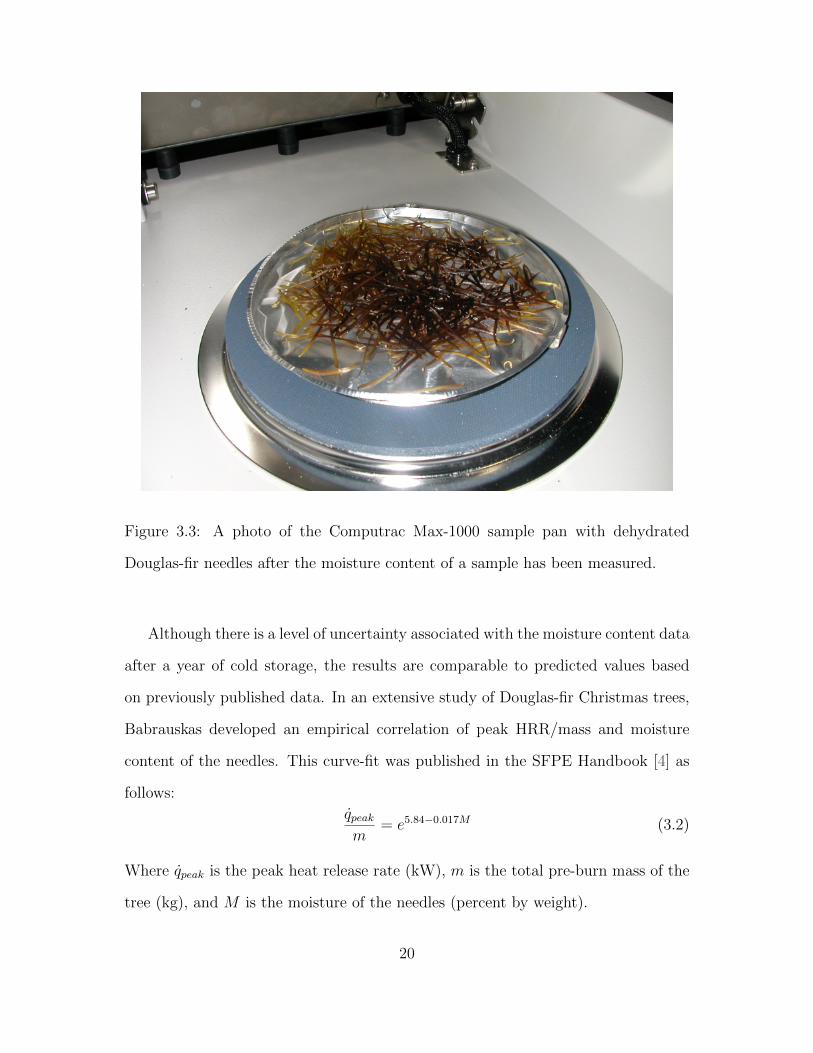
Figure 3.3: A photo of the Computrac Max-1000 sample pan with dehydrated

Douglas-fir needles after the moisture content of a sample has been measured.

Although there is a level of uncertainty associated with the moisture content data

after a year of cold storage, the results are comparable to predicted values based

on previously published data. In an extensive study of Douglas-fir Christmas trees,

Babrauskas developed an empirical correlation of peak HRR/mass and moisture

content of the needles. This curve-fit was published in the SFPE Handbook [4] as

follows:

q̇peakm

= e5.84−0.017M (3.2)

Where q̇peak is the peak heat release rate (kW), m is the total pre-burn mass of the

tree (kg), and M is the moisture of the needles (percent by weight).

20

The data for the curve-fit equation is based on averaged moisture contents from

samples taken at both inner and outer branches; samples for this study were taken

only from outer branches. Figure 3.4 compares Babrauskas’ data using both the

averaged moisture content values and those taken from outer branches only, to that

obtained from this series of tests. The moisture content and HRR/mass data ob-

tained here fits reasonably well within the spread of data points, lending confidence

to the values of moisture content obtained from the frozen samples.

21

Figure 3.4: Peak HRR/mass from Douglas-fir trees as a function of moisture content

showing the curve-fit line developed by Babrauskas and the data used in deriving

it (circular data points), as well as data obtained during this study (triangular

data points). Also shown are the three moisture content regimes – MC<30% ,

30%<MC<70% and MC>70%, indicated by vertical dashed lines.

The moisture content analyses are also in agreement with previous research done

22

by Chastagner, who found that Douglas-fir trees with a moisture content of 30%

or less will be fully consumed, those with a moisture content of 30-70% are in

the transition range where the tree will likely be partially consumed if successfully

ignited, and trees with>70% moisture content will not sustain burning [5]. The trees

tested in this study are divided into these three regimes, MC<30%, 30%<MC<70%

and MC>70%, with regime 1 being the most dry and regime 3 being too wet to

sustain burning. These regimes are also indicated in Figure 3.4 by the vertical

dashed lines.

Tree 12-1 (the third tree burned) was visually much more green than the other

trees, due to its relatively high moisture content (regime 3), and exhibited different

combustion behavior from the other eight trees. It was never fully involved and large

portions remained unburned after the test. Because it could not sustain burning,

the results for that test are not included in segments of the analysis that are based

on complete consumption of the needles. However, this burning pattern is indicative

of what would be expected from trees that have not been excessively dried before

testing or have not experienced a severe drought condition, and the comparatively

low peak HRR for a tree of that size fits well with the curve-fit line mentioned

previously.

3.2.2 Mass loss

The trees lost an average of 50% of their pre-burn mass during the combustion phase;

the moisture content determined how completely a tree would burn. Figure 3.5

shows the effect of the moisture content of the needles on the mass loss, although it

is not a precise means of predicting burned mass. The percentage of mass consumed

was calculated by dividing the total mass lost (as reported by the load cells) by the

total initial mass, which necessarily includes the tree trunk. However, the trunk does

23

not contribute significantly to the mass loss, as it forms char and resists burning.

By far, needles and small stems represent the bulk of mass lost, although this is

not quantified. Based on a visual analysis of the trees post-burn, 90-100% of the

needles are consumed when the tree is very dry, i.e., in MC regime 1. This loosely

correlates to 50-60% of the total mass, but is dependent on a particular tree’s ratio

of burnable mass (needles) to unburnable mass (trunk).

24

Figure 3.5: The role of moisture content on the percentage of mass consumed show-

ing how different regimes affect the percentage of mass consumed, with a linear

curve fit overlaid on the data.

25

Table 3.2: Recorded values for all trees, including mass, peak HRR, mass loss andmoisture content

Tree Weight Mass MoistureTree HRRpeak Pre-burn Mass Loss Consumed Content MC Regime

(kW) (kg) (kg) (%) (%)4-1 778 2.85 1.44 51 25.21 14-2 719 1.549 1.04 67 14.75 14-3 1661 4.372 2.67 61 15.01 18-1 3347 17.6 9.13 51 43.87 28-2 3402 17.64 8.6 49 53.57 28-3 5035 28.75 12.53 44 23.57 112-1 855 29.92 3.265 11 93.42 312-2 4976 31.92 13.49 42 61.00 212-3 4007 29.14 7.91 27 54.61 2

3.2.3 HRR

Figure 3.6 provides a plot of the measured HRR curve for each of the trees burned.

For some of the trees, there was a significant delay between the start of the test when

the ignition source was applied, and established burning, leading to a staggered

appearance of the curves. Established burning is defined as the time at which the

fire starts to rapidly grow towards its peak and an ignition source is not needed.

Based on this definition, trees in moisture content regime 1 reached established

burning in 1 to 7 seconds whereas trees in regime 2 and 3 required a longer growth

period of 8 to 27 seconds.

26

Figure 3.6: HRR plotted over time of the nine trees burned in the first phase of

testing, from start to 120 seconds which encompasses the entire burn from ignition

to flame-out.

The experiments demonstrated that there is a similarity in the shape of the HRR

curves from start to peak HRR among all the trees. All trees required approximately

30 seconds to reach peak HRR from established burning, regardless of height or mass.

Figure shows the HRR curves transposed to align the peak HRR at 30 seconds. From

this figure, it is apparent that the size of the tree plays a large role in determining

the peak HRR for the dry trees, but has a negligible effect on the total burn time.

Tree 12-1 was the exception to this general rule, as its peak HRR was comparable

to that of the 4 foot trees. However, this is to be expected due to its unusually high

moisture content (93%) relative to the other trees, placing it into moisture content

27

regime 3.

Figure 3.7: HRR curves from the 9 trees burned in the first phase, aligned so

that the peak HRR occurs along the same vertical axis, allowing a direct visual

comparison of the rate of increase, which shows that the different sizes of trees all

took approximately 30 seconds to reach peak HRR.

Using 60 seconds as a common time interval for burning, the total heat released

by the Douglas-fir trees can be approximated by a triangle, as demonstrated in

Figure 3.8 for two of the measured HRR curves. The area of the triangle (0.5 ·

60 s · peak HRR) compares favorably to the actual area under the measured HRR

curve (total energy released in kJ), as seen in Figure 3.9. Although more testing is

required to determine if other tree species can be approximated in this manner, the

methodology does provide a simple way to determine the total heat released during

28

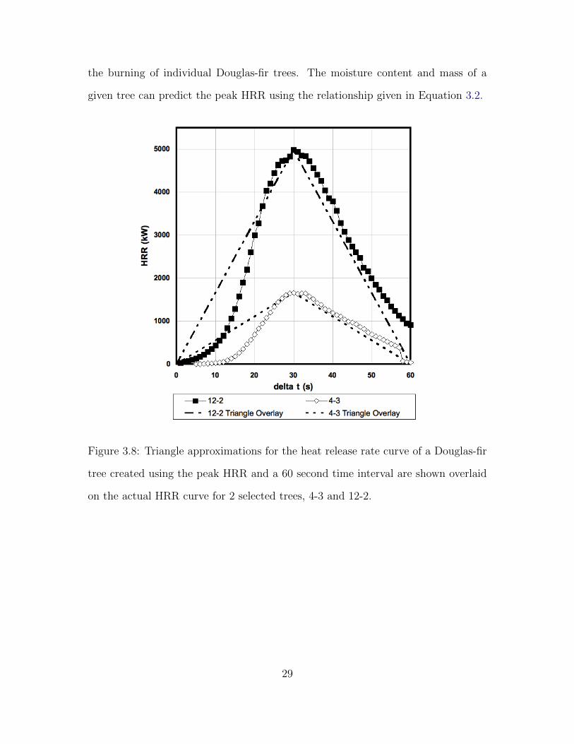
the burning of individual Douglas-fir trees. The moisture content and mass of a

given tree can predict the peak HRR using the relationship given in Equation 3.2.

Figure 3.8: Triangle approximations for the heat release rate curve of a Douglas-fir

tree created using the peak HRR and a 60 second time interval are shown overlaid

on the actual HRR curve for 2 selected trees, 4-3 and 12-2.

29

Figure 3.9: This chart shows the agreement between the measured value of energy

released, and the triangle approximation used to calculate heat released by means

of the peak HRR and a 60 second duration.

3.2.4 Tree Mass as a Function of Height and Leaf Area

To predict the peak HRR and total heat released of Douglas-fir trees by means of

Equation 3.2 and the triangle approximation the mass must be known or estimated.

The mass is a function of the tree’s age and trunk diameter, the density of the needle

growth, height and moisture content; as such, mass can be difficult to estimate for

trees that have not been harvested. A preliminary methodology to estimate tree

mass uses the tree’s crown height (as detailed in section 3.1.2). This simplistic

30

approach relies on the relatively uniform axis-symmetric shape of Douglas-fir trees.

For trees with uneven growth patterns and deciduous trees, a more rigorous approach

will be needed.

Calculating mass from leaf area may be viable across a wider range of tree

species. Leaf area is a measure of the surface area of a tree’s crown occupied by

leaves or needles and is utilized to predict a tree’s behavior in such areas as pollu-

tion interception, rainfall storage and CO2 sequestering [20]. The trunk and large

branches do not play a large role in individual tree fires; therefore the leaf area is a

logical indicator of burnable mass and fire size. Another commonly used measure is

the surface area to volume ratio, or σ, which defines the density of foliage and can

describe how flammable a plant may be, in conjunction with moisture content [27].

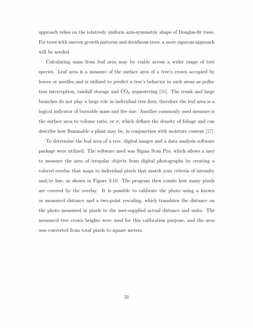
To determine the leaf area of a tree, digital images and a data analysis software

package were utilized. The software used was Sigma Scan Pro, which allows a user

to measure the area of irregular objects from digital photographs by creating a

colored overlay that maps to individual pixels that match your criteria of intensity

and/or hue, as shown in Figure 3.10. The program then counts how many pixels

are covered by the overlay. It is possible to calibrate the photo using a known

or measured distance and a two-point rescaling, which translates the distance on

the photo measured in pixels to the user-supplied actual distance and units. The

measured tree crown heights were used for this calibration purpose, and the area

was converted from total pixels to square meters.

31

Figure 3.10: A screenshot from the software program used to create and count

colored pixel overlays which are used to calculate leaf area. In this example the pixels

that meet criteria of color and hue matching those of the needles are highlighted

and counted, allowing surface area to be measured for irregular-shaped objects such

as trees.

Figure 3.10 illustrates the overlay applied to tree 4-1 to measure the area of

32

needles from a photo. In the given example, 199768 pixels were counted, which

translates to 0.583 m2. The tree has a crown height of 1.37 m, which is equal to

806.8 pixels in the original picture, giving a calibration factor of 0.1709, or 100 pixels

= 0.1709 m. In order to translate a sum of pixels to square meters the following

equation is used:

Area = pixels ∗ 0.17

100

2

(3.3)

The area was obtained in this manner two times for each tree burned, from two

photos taken 90◦ relative to one another, and then averaged, which should account

for any lopsided trees.

A comparison of the two methods for estimating mass, leaf area and crown

height, in Figure 3.11 shows that using the leaf area as a means of predicting mass

has a slightly higher R2 value than using the crown height (0.91 vs. 0.87)1. Using

the leaf area method of estimating mass also has potential applicability to other

species, and for this reason would be recommended over using the tree height for

future applications. However, in the case of the Douglas-fir trees tested in this study,

the leaf area method tends to over predict mass, which in turn leads to higher than

measured peak HRR predictions.

1An R2 value, also known as the coefficient of determination, is a number from 0 to 1 used toindicate how closely a trendline corresponds to the data is it created from, where 1 would indicateperfect agreement between data points and a trendline.

33

Figure 3.11: Comparison of the relationships between crown height, leaf area and

tree mass for use in estimating mass by means of a trendline from either leaf area

or crown height data.

3.2.5 Imaging (Flame Characteristics)

Figure 3.12 presents a timeline of images captures at five-second intervals centered

on the time of the peak HRR. The fire growth rate visible in the stills taken from

34

video recordings of the experiments (tree 12-2 was not taped) shows the similar

times to peak HRR from ignition, as was indicated in Figure 3.7.

Figure 3.12: Fire video image-captures arranged by 5 second centered around the

time of peak HRR showing the progression from ignition to peak is nearly the same

time scale in all tree fires regardless of tree size.

The mean flame height, Hflame, was determined for each experiment by analyzing

video and still photos showing the burning tree, using the thermocouple tree as a

reference. The flame height (see Figure 3.13) is the distance from the base of the

flame near the tree bole to the top of the flame where the flame intermittency is

0.5, at which height the flame is visible 50% of the time. Still photographs were

used to determine the flame height, in conjunction with the video record showing

flame intermittency. In the case of this study, the mean flame height, Hflame, differs

35

slightly from the flame height L that is common in the literature, in that included in

the height is the burning fuel package. It is difficult to provide direct comparisons

to flame height calculations that are based on the flame height above the fuel, which

is in many cases a gaseous diffusion flame, or crib fire. To model a fire’s impact on

its surroundings in the WUI, it makes little sense to disregard the flaming portion of

the tree and focus only on the flame extending above it; however, if a value for L is

needed, it would merely be the flame height Hflame minus the crown height Hcrown.

36

Figure 3.13: Flame height graphic showing how the mean flame height was derived

from analysis of digital photos. The thermocouple tree was used as a reference

point, as each thermocouple was at a known height, and the mean flame height

was the distance measured from the base of the fire to the top of the flame where

intermittency was 0.5.

37

A linear relationship was found between the crown height and the ratio of the

flame and crown heights, with the largest ratios resulting from the smallest trees

(see Figure 3.14). Depending on tree size, the flames were, on average, twice the

height of the tree crown. Trees with a crown between 1 and 1.5 meters, however,

will have a mean flame height that is roughly three times that. Predicting flame

height, in conjunction with a flame temperature, enables calculation of the radiative

heat flux to which a nearby structure may be exposed.

38

Figure 3.14: Flame height data showing relationship between crown height and the

ratio of flame height to crown height which shows that trees will have flame heights

between 1.5 to 3 times the crown height, depending on tree size.

39

Table 3.3: Data table showing the tree heights, and the flame heights as calculatedfrom digital photographs

Hcrown FlameTree (m) Heigh(m)4-1 1.3716 4.24-2 1.2954 3.474-3 1.4224 4.368-1 2.3114 4.618-2 2.6162 5.058-3 2.4384 5.6112-1 3.0988 N/A12-2 3.2004 5.0812-3 3.3274 4.69

3.2.6 Flame Temperatures

The temperature of the fire and plume was measured via seven thermocouples from

0.6 to 4.3 meters above the tree base. The peak temperatures were usually measured

by either TC6 or TC7, which are the lowest two thermocouples, located 0.6 and 1.2

m above the tree base, respectively. This is the height at which the tree has the most

needles and is also at its widest, which leads to a higher volume of dead needle and

twig material in the interior of the tree. Table 3.4 shows the recorded peak values

and locations as well as the measured temperature at the highest thermocouple,

TC1.

40

Table 3.4: Peak flame temperatures and the location they were measured, as well as

the temperature measured at TC1 which was the highest thermocouple located 4.3

m above the tree base. Average temperature is the average of the peak temperatures

recorded at each of the 7 thermocouples for a given test discounting those below the

seat of the fire.

Tree Peak Temp Location TC1 Average

(C) of Peak (C) (C)

4-1 803 TC6 117 402

4-2 730 TC7 226 535

4-3 910 TC7 246 554

8-1 1010 TC6 409 674

8-2 914 TC6 449 675

8-3 997 TC6 598 776

12-1 458 TC2 366 337

12-2 967 TC5 572 744

12-3 677 TC5 448 525

The plume temperature can be characterized by TC1, which at a height of 4.3

meters was well above the areas of intense burning on even the tallest trees. It is

difficult to pinpoint the base of the fire, as it varied from tree to tree, but it was

typically at or around the lowest thermocouple, TC7 at 0.6 meters. That would

make the plume temperature as measured by TC1 at the height of 3.7 meters above

the seat of burning. If Tree 12-1, which did not fully ignite, is discounted, a clear

relationship between peak HRR and plume temperatures can be seen in Figure 3.15.

41

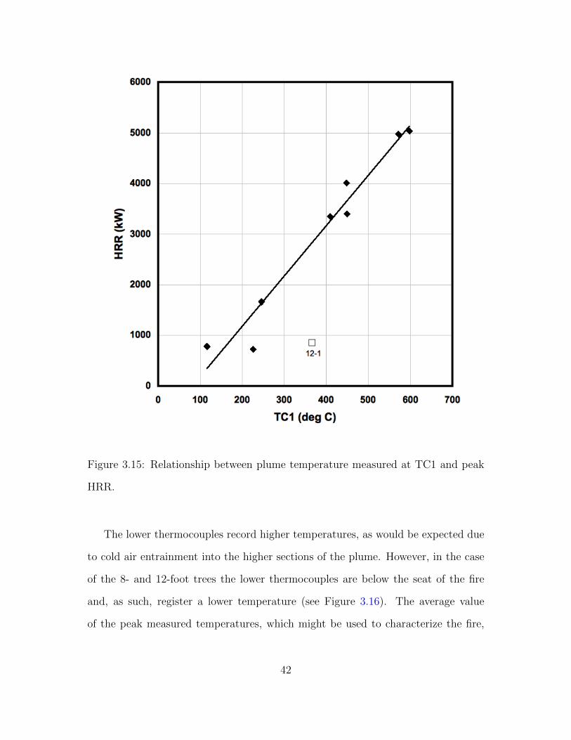
Figure 3.15: Relationship between plume temperature measured at TC1 and peak

HRR.

The lower thermocouples record higher temperatures, as would be expected due

to cold air entrainment into the higher sections of the plume. However, in the case

of the 8- and 12-foot trees the lower thermocouples are below the seat of the fire

and, as such, register a lower temperature (see Figure 3.16). The average value

of the peak measured temperatures, which might be used to characterize the fire,

42

is presented in Table 3.4. The averages do not include the temperatures recorded

below the seat of the fire.

Figure 3.16: Peak temperatures measured at each thermocouple station, where TC1

is the highest thermocouple, and TC7 is the closest to the tree’s base.

3.2.7 Heat Flux

Structure ignition in a WUI zone can result from any of several sources, such as

burning brands (airborne embers that can be lofted a great distance ahead of a

43

flame front), convective heating (when a flame or fire plume actually impinges upon

a structure), or radiative heat transfer. Although radiation from a single burning

tree to a nearby structure is not likely to cause ignition, it can still enhance fire

spread by pre-heating the structure, which lays the groundwork for ignition from an

airborne brand.

For the first two tests (4-1 and 8-1), six heat flux gauges were in place to measure

the incident flux within 3 meters of the burning tree. Starting with test 3, a seventh

heat flux gauge was added at a distance of 10m from the trees to capture total

radiation. The measured peak incident heat flux values for all seven gauges are

shown in Table 3.5. Referring back to Figure 3.1, the arrangement is such that

gauges 1 through 4 were arranged vertically at a distance of 3.1 meters from the

centerline of the tree, at different heights. Gauge 1 was 4.3 meters above the tree

base, and gauge 4 was 0.6 meters above the base. Gauges 5 and 6 faced upwards

at ground level 1.6 and 3.1 meters from the tree centerline to record the heat flux

experienced by grasses or shrubs in the vicinity of the tree. Gauge 7 was located at

a distance of 10 meters.

Table 3.5: The peak values recorded at each of the seven radiant heat flux gaugesare shown here for each tree burned.

Gauge 1 Gauge 2 Gauge 3 Gauge 4 Gauge 5 Gauge 6 Gauge 7Tree kW/m2 kW/m2 kW/m2 kW/m2 kW/m2 kW/m2 kW/m2

4-1 1.26 1.62 2.04 1.98 0.80 1.88 N/A4-2 1.14 1.38 1.76 1.69 0.72 1.71 0.174-3 3.82 4.60 4.81 4.33 2.08 3.96 0.508-1 4.12 4.96 5.55 5.08 2.54 5.21 N/A8-2 4.54 5.12 5.72 4.88 2.58 5.14 0.558-3 9.21 9.21 8.68 7.44 4.27 7.65 0.0012-1 1.64 1.88 1.74 1.06 0.70 0.78 0.1112-2 5.88 6.56 6.45 4.66 2.93 3.79 -0.0112-3 4.91 5.09 4.73 3.39 2.35 3.49 0.50

44

To predict heat flux from a burning tree, characteristics of the flame itself are

needed: height, diameter and temperature. Flame height is a function of tree height

and moisture content, and the width is fairly constant. Once the dimensions and

temperature of a flame are known, the radiation from the flame can be calculated

to predict the flux from a single burning tree to a nearby structure. By treating the

flame as a 2-dimensional rectangle oriented towards a large receiver, such as a wall,

the incident flux can be calculated by using Equation 3.4.

q′′ = F · ε · σ · T 4f (3.4)

where q′′ is the incident heat flux in (kW/m2), F is the view factor, ε is the flame

emissivity, σ Stefan-Boltzman constant (K4kW/m2), and T is the flame temperature

(K). Assuming an emissivity of one and treating the flame as a black-body emitter

will produce the most conservative estimates. The view factor, or configuration

factor, takes into account the distance and orientation of the receiver with regards

to the emitter.

As an example, for tree 8-2, which has a flame height of 5 m and a width of 0.8

m (both determined using the scaling technique shown in 3.13), the configuration

factor to calculate radiation from a rectangle to a parallel small element of surface

dA works out to be 0.096. Using the average flame temperature of 675 C, or 948

K, the incident heat flux is calculated to be 4.4 kW/m2 at the height of 2.7 meters,

which corresponds most closely to heat flux gauge 3, which recorded 5.72 kW/m2.

However, if the temperature recorded at thermocouple 5 (791◦C) is used instead

of the average temperature, the result increases to 6.9 kW/m2. The appropriate

value is likely between these results. TC5 represents the temperature at the very

dry needles in the center of the fire plume and not the gas temperature at the

boundary of the flames, which would be lower due to entrained air. This is one

45

of the limitations of using a 2-dimensional rectangle to model heat flux: choosing

an appropriate flame temperature (This issue remains when modeling the flame as

a cylinder.) As an initial attempt to predict the incident heat flux with known or

estimated values of temperature and dimension, the two-dimensional model provides

a rough estimate.

Figure 3.17: The peak incident heat fluxes recorded for all seven gauges which were

located at positions oriented horizontally and vertically relative to the fire.

46

To measure the total flux, the remote heat flux gauge was able to see most of the

flame, as opposed to the gauges located 1m away from the burning tree. Treating

the flame as a point source, total flux was calculated for a sphere, so the measured

heat flux was multiplied by 4πr2. The heat flux was measured 10 meters from the

base of the tree, the distance r was calculated from the gauge to the tip of the tree,

which approximately corresponds to center of the total flame (see section 3.2.5).

These results, along with the peak HRR and calculated contribution to the total

heat released are shown in Table 6. Only four tests of the six had uncorrupted data.

Table 3.6: Heat flux measurements, calculated total heat flux and radiative fraction.

Tree Hcrown(m) Peak HRR (kW) Peak Flux (kW) Radiative Fraction (%)4-2 1.30 720 220 304-3 1.42 1660 670 408-2 2.62 3400 771 2312-3 3.33 4000 760 19

3.2.8 Comparison Across Species

There is a dearth of similar tests involving different species but there is some data

available from seven individual Scotch Pine tree burns which were conducted at

NIST [24] (an eighth tree did not ignite). These experiments were conducted in a

laboratory setting, although the trees were burned in a room-corner configuration,

which would likely lead to slightly higher HRRs due to re-radiation from the corners.

The two sets of data were plotted together in Figure 3.18.

47

Figure 3.18: A plot showing the crown height and peak HRR for two different species

of trees - the Douglas-fir trees tested in this study, and Scotch Pine trees which had

been burned previously in a study on Christmas tree home ignition hazards.

As can be seen, there is considerable scatter amongst the Scotch Pines data

points. The moisture content of the Scotch Pines is not known, but given that they

burned to completion and were readily ignitable, it can be assumed they were in

regime one (very dry trees). Likewise, the height measurements may not match

48

crown height used in this study. Even with these unknowns, it would appear likely

that the results from this study are somewhat applicable to at least one other similar

type of tree, although more tests are required to resolve the amount of scatter present

in the data.

49

Chapter 4

Exposure to Radiant Heat Before

Ignition

The effect of radiant heat transfer upon a structure or plant is dependent on two

aspects – the intensity of incident heat flux, and the duration of said radiant flux.

It was found during the International Crown Fire Modeling Experiment that the

incident heat flux on a structure was 30 kW/m2 from a flame front 28 m away, with

a residence time of one to two minutes. Based on this, it was decided to do extended

low-flux exposures to simulate a brief high-intensity one, due to the inability to safely

produce 30 kW/m2 in a lab setting. In order to simulate the effect of an encroaching

wildfire, an electric radiant panel located 60 cm from the tree was used to expose

the trees to approximately 2.5 kW/m2 radiant flux for various timescales prior to

igniting them via a gas burner. The durations used for the tests were 6 minute

exposure, 25 minutes, and 50 minutes, as well as a control group which was not

pre-heated prior to ignition. The intent was not to heat the plants to the point of

ignition, as the radiant heater was not in the part of the fire lab where large-scale

testing can be done, but to see what effect the radiant pre-heating had on the fire

50

characteristics following a piloted ignition.

4.1 Methodology

The trees were again burned in the National Institute of Standards and Technology

(NIST) Large Fire Laboratory under the largest calorimeter hood. Prior to ignition,

the trees were exposed to various durations of heat flux to measure the impact of

radiant pre-heating. While the trees were exposed to the radiant panels, the mass

loss was recorded, to determine the rate of evaporation.

4.1.1 Instrumentation

Thermocouples were placed on a thermocouple tree such that the tips are in the

foliage of the trees, as shown in Figure 4.1. There were 8 in total, spaced at 30

cm above the platform level and then every 20 cm thereafter, except for the eighth,

which was at 200 cm above platform level.

51

Figure 4.1: Experimental setup for the tree burns after the trees have been exposed

to radiant panels showing thermocouple tree and load cell located under hood.

Figure 4.2: Diagram of the heat flux gauges 1 through 3 at the platform under the

calorimeter hood where the trees were burned, located 1 m, 2 m and 10 m from the

tree center.

52

Three heat flux gauges at a height of 1 m were placed near the tree when it was

being burned. One was located 1 m from the center of the tree, one 2 m, and one

10 m, as shown in Figure 4.2. The gauge located 2 m from the tree was slightly

offset to allow a clear line of sight to the tree without the 1-m gauge interfering.

Two more gauges recorded the incident heat flux at the radiant panel while the

trees were being pre-heated – one was placed near the tree’s trunk to measure the

penetration through the branches, and the other was located behind the tree, as

shown in Figure 4.3.

Figure 4.3: Diagram showing locations of the two heat flux gauges at the radiant

panel; one in place behind the tree, and one next to the trunk of the tree.

53

There were a total of two load cells used in these tests. One, known as the Burn

Load Cell, was located under the calorimeter hood where the trees are ignited, and

used to measure mass loss rates during burning and instantaneous mass of the tree

before and after exposure to the radiant panel. The second load cell, referred to

as the Radiant Panel Load Cell, was located directly in front of the radiant panel.

This was used to measure the mass lost as the trees were dried by the panel. The

readings from the load cell were recorded by hand on a time step of 30 seconds for the

duration of the radiant exposure. There is some error associated with absolute mass

recorded at this load cell due to its low height, as some of the trees had branches

that rested on the floor. For this reason, the Burn Load Cell was used to record

the beginning mass and final mass before and after exposure for consistency and

accuracy, and the Radiant Panel Load Cell was used only for mass loss purposes.

The radiant panels utilized for the drying portion of the test procedure were angled

inward approximately 20 degrees with a 10 cm gap between them. Each panel

measures 36.4 cm wide by 198.1 cm tall, and the total distance from the left edge

of the left panel to the right edge of the right panel was 83 cm. The bottom of the

radiant panels was 15 cm off the floor, as shown in Figure 4.4 (a).

54

Figure 4.4: Diagram showing locations of the two heat flux gauges in place behind

the tree, and next to the trunk of the tree at the radiant panel.

The radiant panel was set at approximately 430◦C, and the trees were adjusted

so that the widest portion was approximately 61 cm (2 ft) from the furthest point

on the radiant panels (see Figure 4.4 (b)).

Before the testing began, a flux map was created at the radiant panel, to deter-

mine the incident heat flux at different locations in front of the panels, as shown in

Table 4.1. At a distance of 60 cm from the panels, the incident heat flux was mea-

sured every 15 cm from the base of the panel to the top, with the gauge centered in

55

Table 4.1: Heat flux map created at different points in front of the radiant panels.Heat flux measurements were taken at 13 different heights along the centerline at .6m distance and, and 3 additional measurements were taken, two 30 cm off-center,and one at .9 m distance.

Reading # Vertical Distance from Horizontal Heat FluxPosition (m) Panel (m) Position (kW/m2)

1 .30 .60 Centered 2.752 .45 .60 Centered 2.913 .60 .60 Centered 3.044 .75 .60 Centered 3.085 .90 .60 Centered 3.086 .105 .60 Centered 3.057 .120 .60 Centered 3.028 .135 .60 Centered 3.019 .150 .60 Centered 2.9310 .165 .60 Centered 2.7511 .180 .60 Centered 2.4912 .195 .60 Centered 2.0313 .75 .60 Centered 3.1314 .75 .60 .30 m left 2.5315 .75 .60 .30 m right 2.5916 .165 .90 Centered 1.75

front of the panels. Additionally, two readings were taken 30 cm off-center, and one

at 90 cm distance and a height of 165 cm. The largest heat flux of 3.08 kW/m2 was

measured at 75 cm above the bottom of the panel, as well as at 90 cm. The lowest

heat flux at the top of the panel and a distance of 60 cm was 2.03 kW/m2, and was

2.75 at the base. The average recorded value across all heights at the distance of

60 cm (the distance the tree was located from the panels) was 2.58 kW/m2. At the

height of 75 cm, and 60 cm from the panels where the largest heat flux was recorded

(when centered on the panels) the values 30 cm off-center left and right averaged

2.56 kW/m2.

56

4.1.2 Procedure

The trees were trimmed at the base of the trunk to obtain a level surface, and held

upright by means of screws into a plywood stand that was 2 foot square. The stand

was weighed before attachment, and its mass was subtracted from tree mass or mass

loss calculations. A front face of the tree was chosen based on which side looked

most uniform and didn’t have a noticeable lean that would place sections too close

or distant from the radiant panels, and was marked as such on the plywood stand

as shown in Figure 4.5. The letters A, B, C and D were used when the trees were

being photographed to indicate which face was being photographed.

Figure 4.5: Labeling convention for tree faces used when photos were taken of all

sides of the trees before the exposure to the radiant panel, and after the burn was

completed.

The trees were then photographed in front of a gridded backdrop (Figure 4.6) to

facilitate measuring the leaf area from digital photos. The trees were photographed

from 4 directions, rotating 90 degrees each time, and the photos were labeled A

through D in accordance with Figure 4.5.

57

Figure 4.6: This photo shows the gridded backdrop used for photos so that the area

of the trees could be later measured using a computer software program.

To obtain the moisture content prior to testing, samples of needle clusters were

taken. The samples were taken from the new growth needles on the ends of the

branches in 2-3 inch lengths, with each sample being comprised of three or four

branch tips. Samples were taken from 3 points on the front face of each tree corre-

sponding to the top, middle and bottom thirds, and three corresponding points on

the back face as shown in Figure 4.7. A seventh sampling was taken from the front

middle section consisting of older growth needles located on the middle of the branch

to measure penetration into the tree from the radiant panel, and compare overall

moisture differences between new and old needles. Needle samples, once collected,

were either tested immediately with the moisture content analyzer, or sealed in an

air-tight bag to be tested at the end of the day.

58

Figure 4.7: Sampling points for the needles taken to measure moisture content are

shown here. Samples were taken from the bottom, middle, and top thirds of the

tree, labeled as points 1, 2 and 3, from the front and rear faces of the tree.

After samples were taken for moisture content testing, the tree was placed on

the Burn Load Cell and the weight recorded. Then it was moved to the Radiant

Panel Load Cell and placed so that the front of the tree faced the panels. The

pre-exposure mass was recorded as the starting point for the mass lost over the

duration of exposure. While the mass was being recorded, the tree was shielded

from the radiant panel by a section of sheetrock on a movable track. The radiant

59

panel was at full operational temperature for the duration of testing each day, so

there was no delay from the start of the timed exposure to the desired heat flux. At

the point when the timed exposure began, the sheetrock shielding the front of the

panel was slid back exposing the tree.

There were two video cameras recording at the Radiant Panel, one of which

recorded infrared images. A heat flux gauge located on the far side of the tree

measured the permeability of the plants; or how much radiant heat flux was able to

pass through the foliage.

When the timed exposure was completed, the final mass was noted and the tree

was moved back to the Burn Load Cell, where the mass is recorded again, and needle

samples were taken to compare the moisture contents before and after heating. The

samples were taken from the same locations on the front and back face of the tree

as done previously. The mass was recorded again after the sampling process was

complete.

For the start of the burning section the tree was placed in the burner with the

previously-established front facing towards the bottom of the U shaped methane

burner. The burner consists of approximately 2 cm diameter stainless steel piping

in a U shape with 46, 2 mm holes drilled every 2 cm that flows around 25 liters per

minute to produce a 15-kW ignition source (see Figure 4.8). The gas piping was

supported by a low platform to the side of the load cell and drywall the tree was

placed on, as shown in Figure 4.9.

60

Figure 4.8: Plan view diagram of methane burner used for ignition of trees.

61

Figure 4.9: Side profile diagram of gas burner used for ignition of trees, also showing

the position of the tree relative to the burner when in place for ignition.

The three cameras recording the test from different vantage points, two regu-

lar and one infrared, were activated prior to ignition. At the start of the test the

valve controlling gas supply to the burner was opened, and the burner lit with a

propane torch. The flames reached approximately 12 cm tall and reach the low-

ermost branches, simulating a grass fire that might ignite a landscaping tree, as

shown in Figure 4.10. The burner remained on for 2 minutes. When the tree was

completely finished burning, the final mass was recorded from the Burn Load Cell.

62

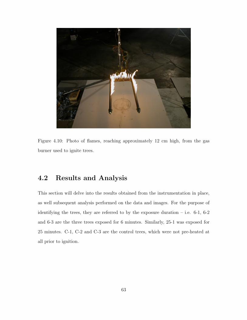
Figure 4.10: Photo of flames, reaching approximately 12 cm high, from the gas

burner used to ignite trees.

4.2 Results and Analysis

This section will delve into the results obtained from the instrumentation in place,

as well subsequent analysis performed on the data and images. For the purpose of

identifying the trees, they are referred to by the exposure duration – i.e. 6-1, 6-2

and 6-3 are the three trees exposed for 6 minutes. Similarly, 25-1 was exposed for

25 minutes. C-1, C-2 and C-3 are the control trees, which were not pre-heated at

all prior to ignition.

63

4.2.1 Moisture Content

For this group of tests, an Arizona Instruments Computrac Max2000XL moisture

analyzer was used, in place of the Max1000 used earlier. The instruments share

the same hardware and algorithms, the only difference being extra features and

export options available with the 2000XL, which were not used. For the purpose of

classifying the moisture content regime, the samples taken from the middle section

of the front of the trees were used, as the trees in the first test series were sampled

from that location. The differences in moisture content from the top section of the

trees to the bottom was noticeable, with the top branches being lower in moisture.

On average, samples taken from the top third of the trees had 93% of the moisture

content from the lower samples. However, all samples taken were in excess of 130%

moisture content, placing the trees well into regime 3. Figure 4.11 depicts the

moisture content from samples taken from the front middle section of each tree

before and after being exposed to the radiant panel for different lengths of time.

Trees that experienced 6 minutes exposure did not lose a significant amount of

moisture. However trees that were exposed for the longer periods of time, 25 and 50

minutes, lost between 17% to 75% of their moisture from the middle-front section

with the most extreme case belonging to the third tree in the 50-minute set.

64

Figure 4.11: Bar graph showing the measured moisture content from samples taken

from the front middle section of the trees before and after exposure to the radiant

panels for differing lengths of time.

The average for the 25-minute set was a loss of 30%, whereas the average was a

50% reduction in moisture over 50 minutes. However, these reductions in moisture

content only reflect the front center section of the tree, which was expected to be the

most effected by the preheating. The other sections of the trees were also sampled

and tested to discover how much heat would pass through the trees foliage, for

instance. The moisture contents obtained from the front top and bottom samples

showed similar rates of drying compared to the middle section. The back side of

the tree, however, showed little to no signs of dehydration. Figure 4.12 shows the

percentage drop in moisture content for all six sampling points from the 9 trees

exposed to the radiant panel. The error associated with measuring the moisture

content is likely around 5% due to variation among needles and twigs. Samples

65

taken from the back side of the tree before and after they were exposed to the

radiant heat show a loss of at most 5%, and in some cases a gain in moisture

content. Given the range of error, and an average across 27 samples of a 2.5% loss,

it seems evident that there was no appreciable effect on the far side of the tree in

terms of moisture loss due to radiant heat flux, in particular given the trees’ high

moisture content starting point.

66

Figure 4.12: The percentage drop in moisture content for 9 trees sampled in 6

different places - three on the side facing the radiant panel, and three on the far side.

Samples taken from the back side of the tree showed negligible drops in moisture

content.

From the fact that only half the tree was affected by the pre-heating, it is difficult

to determine exactly what the overall moisture content of each tree was at the time

they were burned. Taking the average of the six sampling points will provide at

least an idea, however. The average of all points sampled after the pre-heating is

presented in Table 4.2, with the exception of C1, C2, and C3, which as the control

67

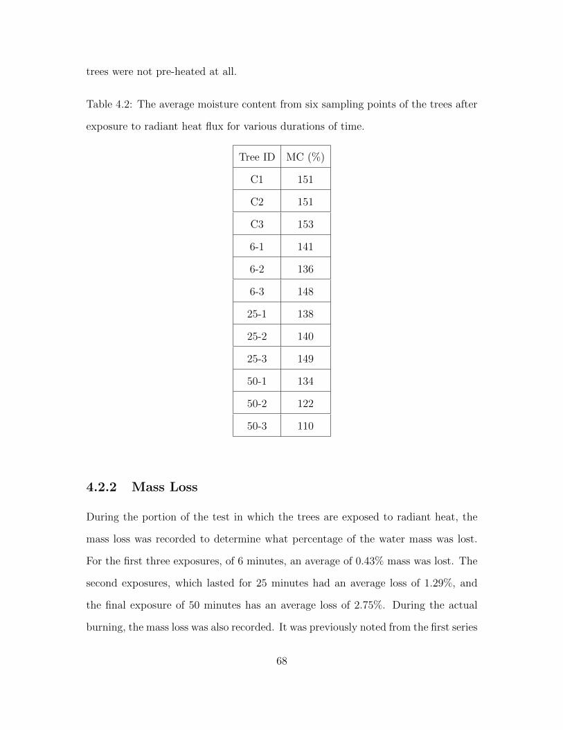
trees were not pre-heated at all.

Table 4.2: The average moisture content from six sampling points of the trees after

exposure to radiant heat flux for various durations of time.

Tree ID MC (%)

C1 151

C2 151

C3 153

6-1 141

6-2 136

6-3 148

25-1 138

25-2 140

25-3 149

50-1 134

50-2 122

50-3 110

4.2.2 Mass Loss

During the portion of the test in which the trees are exposed to radiant heat, the

mass loss was recorded to determine what percentage of the water mass was lost.

For the first three exposures, of 6 minutes, an average of 0.43% mass was lost. The

second exposures, which lasted for 25 minutes had an average loss of 1.29%, and

the final exposure of 50 minutes has an average loss of 2.75%. During the actual

burning, the mass loss was also recorded. It was previously noted from the first series

68

of tests that the very dry trees in moisture content regime 1 and 2 lost anywhere

from 27% to 67% of their starting mass. The trees in this series remained at high

enough moisture content even after pre-heating that the did not fully burn, and lost

an average of 6.1% of their total mass during the burn phase.

4.2.3 Heat Release Rates

The heat release rate curves for the trees burned in this phase of tests exhibited a

different pattern than those discussed in the previous chapter. Due to their higher

average moisture content, placing them well into regime three (as defined in section

3.2.1) which translates to a low probability of sustained burning they did not burn

to completion; rather, only a small quadrant of the tree would burn and then self-

extinguish. However, in six of the tests, after the first die down the tree would

briefly flare up again to produce a second HRR curve, which typically had a lower

peak value and shorter duration than the first one. In one instance, the second peak

was larger. The second-peak phenomena was most likely as a result of the burner

remaining on and progressively drying to lower branches until a second flare-up

occurred. As noted by Babrauskas et al. in Flammability of Cut Christmas Trees,

in flammability tests done with 15 cm Douglas-Fir branches, once the samples were

removed from the ignition source if they were in excess of 80% moisture content,

they would self-extinguish with no further flame spread. [5] For this reason, for

the purpose of comparison to the first tree tests which used an ignition source that

was removed as soon as the tree was burning, the second peak was discounted for

analysis. This allowed the trees to be investigated using the same pattern of a single

peak for the purpose of peak HRR and total heat released.

The first step to calculate the peak HRR and total heat released was to normalize

the HRR plots to account for drift as the testing day continued. Drift occurs as the

69

moisture traps of the calorimeter become saturated and show a falsely elevated HRR

as time continues. In order to account for drift, a moving average is taken 30 seconds

before and after the test ends, and that number is used to set the baseline to zero

kW. In addition to drift, these tests used a methane burner for ignition, so the heat

contributed by the burner needs to be deducted from the total heat. The burner

contribution is a known value, and that amount is deducted from the HRR. This

produces data that reflect the heat contribution of the burning tree only.

70

Figure 4.13: HRR-time curve for a tree that has been exposed to radiant heat for

50 minutes and then ignited, showing the dual-peak phenomenon that some of the

trees exhibited.

Figure 4.13 depicts the dual-peak HRR curve mentioned above. This particular

tree was exposed to approximately 2.5 kW/m2 incident heat flux for a duration of

50 minutes prior to ignition. The individual HRR curves for the remaining 11 trees

tested in this series can be seen in Appendix A. As can be seen from the graph, the

peak HRR was quite low, at only 120 kW for the first peak. This is due to the high

moisture content of the trees, even after a 50-minute exposure, the overall average

71

moisture remained high, and prevented the tree from burning to completion. The

highest peak HRR measured from the trees burned in this series was 312 kW, and

the average peak was 160 kW. This is comparable to the result from the first series,

in which the one tree in regime 3 had a mass twice that of these trees at 38 kg, and

a peak HRR of 855 kW.

4.2.4 Leaf Area

The leaf area for the trees burned in this series of tests was calculated in the same

manner as discussed previously in section 3.2.4. Digital photographs of the trees

were taken before testing, with the addition of a gridded backdrop to aid in scaling

the tree’s height. This is a method less prone to user error, as the original method

relied on having an accurate measurement of the crown height, and being able to

relate that measurement to the photo at hand. The crown height was measured

from the bottom-most branch to the base of the upper shoot, but those points

were at times difficult to establish from the photo. By using the grid to scale the

measured areas, a consistent pixel to actual length relationship was used in each

measurement. Figure 4.14 shows an example tree in front of the backdrop. When

the photo was calibrated, the software program would measure the distance in pixels

between two user-specified points, A and B in this photo, and the actual value in

meters was entered. This produces accurate measurements of the tree’s leaf area in

square meters.

72

Figure 4.14: Photo a one of the trees prior to being burned in front of the grid back-

drop used to calibrate distances in the digital photos for the purpose of measuring

the leaf area, where the distance between ’A’ and ’B’ is known.

Each tree was measured from two different photographs taken at 90◦ rotations

to account for any uneven growth in one direction. These trees, unlike those burned

in the first series of tests, were very similar in height and diameter, and had very

similar leaf areas. The results from this test were plotted against tree mass in

conjunction with the same results obtained from the first trees burned, to further

73

test the validity of the tree mass to leaf area relationship.

Figure 4.15: Chart showing the relationship between leaf area and tree mass for trees

from both the first and second series of tests, which were obtained from different

tree farms.

It can be seen in Figure 4.15 that the data points from this series of tests, denoted

as ’Radiant Heating,’ fall in roughly the appropriate area as compared to data points

from the previous section. However, as an example, for a tree with a leaf area of 1.8

m2 the corresponding mass within the scatter of data could relate to a tree of 11 kg,

or one of almost 25 kg. The problem lies with the different sizes or thicknesses of

74

trunk, which can vary depending on a trees age, health, and also at what height the

tree was cut. However, as the trunk and large branches barely contribute to the fire

size, it is not ideal to base fire size predictions off of something so arbitrary. In the

future, one possibility would be to develop a relationship that eliminated the need

for mass altogether, and instead use leaf area to directly predict HRR and other

characteristics in conjunction with the moisture content.

75

Chapter 5

Fire Spread Amongst Closely

Grouped Trees

The purpose of this series of tests was to determine how readily fire would spread

from one burning tree to a nearby tree, with the variables being tree spacing and

moisture content. All the trees used in this series were the same approximate age,

height and mass. They were obtained from the same tree farm and were cut on the

same day, July 31 2003. The trees were divided into either dry or wet categories.

The former were allowed to air dry inside the large fire lab for the 3 weeks between

when they were cut and testing began on August 21, and the latter were kept

well-watered to keep their moisture content higher. It was found that amongst the

watered trees, some trees retained more moisture than others, as indicated by needle

loss and discoloration. Based on visual observations prior to testing, the trees were

categorized as very dry, moderately dry, or wet.

From needle samples taken at the time, frozen, and later tested (at the same time

as the samples taken from the first tests) the very dry trees has a needle moisture

content of around 15% and the wet trees were around 60%. Based on the moisture

76

content, they can be placed in regime one and two of the moisture content band

as established previously. However, not every tree was sampled, and therefore the

moisture contents must be taken only as in indication of the approximate level of

moisture, not an absolute. The setup for the tests followed a slightly different proce-

dure than the tests described in previous sections. Rather than burning individual

trees, for this phase of testing groups of trees, between two and four at a time, were

burned together. The trees were placed in a line on a diagonal across the platform,

and the spacing between them was changed from test to test but varied from 3 in

to 12 in. The spacing was measured from the widest part of the tree, typically

at about one third of the crown height measured from the base of the tree. The

trees were arranged on a large platform which was supported by 4 load cells, the

readings of which were totaled. This platform was located underneath the large

hood for calorimetry measurements. One heat flux gauge was placed 1.8 m (6 ft)

perpendicular to the centerline the trees were lined up along, as illustrated in Figure

5.1.

5.1 Procedure

The first test consisted of four dry trees, ID numbers 1, 7, 10, and 13, spaced 1 foot

apart in a line. One tree, known as the ignition tree (as denoted in Figure 5.1), was

ignited by means of a propane torch that was held for 3 seconds on the left side of

the trunk at the lower branches, and then 3 seconds on the right side. Although

tree #7 burned vigorously, the fire did not spread to the adjacent tree (#10). Tree

#7 was discarded and the remaining trees were them shifted so that they were only

6 in apart, and tree #10 became the ignition tree. Using the same procedure, tree

#10 was ignited, and again the fire did not spread to the neighboring trees. At that

77

point, tree #13 was ignited with the torch, while still 6 in from tree #1, with the

same result, there was no fire spread. However tree #1 was singed somewhat on the

outermost needles on the side that was closest to tree #13.

Figure 5.1: Experimental setup for fire spread experiments test 1; 4 trees spaced at

1 foot apart

The second test took the unburned tree from test 1, tree #1 which was singed

but not ignited, and placed it next to a new tree (#9) which was also from the

dry group at a distance of 3 in as shown in Figure 5.2. Tree #1 was ignited and

although tree #9 started smoking after 30 seconds, it still did not ignite before tree

#1 self-extinguished.

78

Figure 5.2: Experimental setup for fire spread experiments test 2; two trees spaced

at 3 in

Test 3 involved four new trees, these ones from the moderately dry moisture

content group, set up the same way in a straight line with 0.152 m (6 in) spacing

between trees. Based on the results from the first two tests with no fire spread

using dryer trees, it could be assumed that the fire would not spread in quiescent

conditions, therefore these tests had the addition of a large fan located 3.15 m (124

in) away aimed at the ignition tree to facilitate fire spread, as illustrated in Figure

??. The presence of wind produced a deflection of the fire plume. This deflection

led to ignition of neighboring trees due to either impingement of flames or increased

levels of radiant heat flux due to the flames’ proximity.

79

Figure 5.3: Experimental setup for fire spread experiments test 3; tree spacing at 6

in with inclusion of fan at 3.15 m – diagram not to scale.

Tree #11 was ignited in the same manner as before, with a 3 second application

of the torch to the left side, and a three second application on the right. At the 6

second mark, the fan was turned on. However, the wind velocity was high enough

as to prevent the fire from becoming well-established. The end result was that the

ignition tree did not burn at all on the side closest to the fan, and only weakly on the

leeward side. However, the fire plume did impinge on tree #3 which ignited. Tree

#3, once ignited, burned for 25 seconds with a fire plume which never grew taller

than 0.9 meters due to the wind affect. The fire did not spread beyond tree #3.

Test 4 took the unaffected trees, #8 and #4, and added one more, #12 which was

also moderately dry. For this test, the fan was moved farther away, to a distance of

7.42 m (292 in). The trees remained at 0.152 m spacing as shown in Figure 5.4.

80

Figure 5.4: Experimental setup for fire spread experiments test 4; tree spacing at 6

in, fan at 7.42 m

Locating the fan at a greater distance resulted in fire spread from tree #8 to #4

and the brief ignition of tree #12. The wind speed velocity was not measured at the

time; however, by using the flame angle taken from a video capture, the approximate

velocity can be deduced. Figure 5.5 shows a video capture taken of test number four

from the east camera. The angle between the tree bases and the flame is 69◦. The

east camera was not exactly perpendicular to the trees, so this angle measurement

is likely somewhat skewed. For the purpose of estimating wind velocity, an angle of

70◦ was used.

81

Figure 5.5: Video capture from test 4 showing the flame angle due to wind as flames

spread from tree #4 to tree #12.

G. Heskestad has compiled a chart depicting flame deflection angles for flames

in wind, plotted against a ratio of uw/uoL which is the wind speed over the mean

axial velocity at the flame tip. [13] The data differentiates amongst different L/D

ratios, or flame height to diameter; however, the difference is negligible amongst the

scatter and was not considered here. In order to calculate the axial velocity at the

flame tip, the following equation was used, which calculated the maximum upward

velocity in a fire plume at the intermittent flame (or flame tip).

82

uo(max) = 1.9Q1/5c m/s (5.1)

In the case of test 4, the peak HRR was approximately 1000kW, so the maximum

axial velocity would be 7.5 m/s from the above equation. Using the flame deflection

chart mentioned previously, the wind speed for a deflection of 70◦ (or 20◦ from

the vertical, as the chart is arranged) and plume velocity of 7.5 m/s, the wind

velocity would be in the range of 0.5 m/s to 0.8 m/s. A rule of thumb mentioned

in Introduction to Fire Dynamics is that a wind speed of 2 m/s will deflect a flame

by around 45◦. [13]

Test 5 repeated the setup from test 4, with 6 in spacing, but using three trees

from the ”wet” group, trees #6, #2 and #5 as shown in 5.6 The fan was kept same

distance (7.42 m). Tree #6 was very resistant to ignition, and even with the torch

held in place for 15 seconds, it didn’t sustain burning for more than 20 seconds, with

very small flames. The fire spread through the center portion of the tree, which had

a greater proportion of dead or very dry needles; none of the outer branches burned.

As such, the fire did not spread beyond the ignition tree.

83

Figure 5.6: Experimental setup for fire spread experiments test 5; tree spacing at 6

in, fan at 7.42 m

For the final test, trees 2 and 5 were used again along with tree #15. This test

was to determine if the trees would ignite when exposed to radiant heating from

a 2 MW heptane burner fire in a quiescent atmosphere. The trees were spaced so

that they were located 40.5 in, 64 in, and 85 in from the burner, measured to the

tip of the tree. The burner was located 4 ft above the tree bases. The layout and

dimensions of the experimental setup are shown in Figure 5.7.

84

Figure 5.7: Experimental setup for fire spread experiments test 6 with a 2 MW

heptane burner located next to 3 trees of high moisture content.

85

Figure 5.8: Photo of heptane burner heating a cluster of trees as part of fire spread

experiments.

The burner was ignited and the trees were observed for signs of smoke, needles

growing brown, or flame. At 17 minutes, the tips of the trees were smoking very

lightly, as can be seen in Figure 5.8. At that point, trees #15 and #2 were ignited

via the same propane lighter as used previously. Both trees ignited, however only

the center portions burned, for the most part the outermost potions of the tree were

resistant to burning. Tree #5, which was not directly ignited by a torch showed

signs of singed needles, but did not ignite.

86

5.2 Results and Analysis

The impact of moisture content on heat release rates has been established in the

previous chapter, so it was not analyzed as fully here. The first four trees burned,

encompassed in tests 1 and 2 of this series, were all very dry trees approximately in

regime one of moisture content. All four trees, in the absence of any wind movement,

burned independently with no fire spread, and can be treated as individual tree fires.

The relationship between the tree mass and its peak HRR was compared to the same

data for the 4-foot trees burned in the first series of tests as described in Chapter

3. The trees burned in the two test series were the same species, however they were

obtained a year apart from different tree farms. It can be seen in Figure 5.9 that

the two test series have a large degree of scatter, but a trend is apparent. One

reason that may account for the disparity is that at the lower range of mass for

this species of trees, small trees around 2 kg, the majority of that mass is naturally

the trunk. The trees from the first series of tests had a comparatively low leaf area

versus the trees burned in the final series. Precise leaf areas are not available for the

fire spread tests trees, but they were visually much fuller and more densely needled,

which could account for the somewhat higher heat release rates.

87

Figure 5.9: Comparison of mass and peak HRR for the 4-foot trees burned in the

first series, tree variation and scaling, and last series of tests, flame spread.

Table 5.1 shows the peak HRRs recorded for each test in this series. Test one

was actually composed of three individual tree burns for all intents and purposes;

those are labeled 1a, 1b and 1c. What this table illustrates is the significant decrease

in peak HRR for the wet trees, even in the presence of wind. In the case of tests

three and four, even though two trees were burning instead of one, the peak HRR

was still lower than the very dry trees burning individually.

88

Table 5.1: The peak HRRs for the trees burned as part of the test series on fire

spread.

Tree IDs Test Peak HRR (kw)

Involved in Test

7 1a 1106

10 1b 1277

13 1c 1575

9, 1 2 1018

11, 3 3 905

8, 4, 12 4 993

6, 2, 5 5 -

Test five, which was composed of very wet trees, had such a low HRR that it

did not register on the laboratory equipment. The peak HRR from test six is not

included in the table because the presence of the heptane burner produced a fire

signature an order of magnitude greater than that of the burning trees, making it

difficult to isolate the smaller HRR. However, based on visual observations, even

with preheating from the burner for 17 minutes, the trees did not fully ignite and

would have had very low HRRs.

89

Chapter 6

Uncertainty

In order to properly evaluate the results of the full-scale fire tests and derive con-

clusions based on measured values, the uncertainty of those measurements needs

to be known. Uncertainty can mean many things, but in this case it will refer to

measurement uncertainty, or the level of confidence in the numbers reported here.

Measurement uncertainly can be caused by several factors: human errors in reading

a scale, imperfections in instrumentation that leads to ’systematic’ errors, or random

errors. Additionally, in some cases (for instance HRR) the reported value is not a

direct measurement, but rather a calculated value using several measured values as

input, each of which will have its own associated uncertainty – therefore there will

be some propagation of the uncertainties.

The uncertainty represents the range of probable values around the measured

value within which the actual value being measured most probably lies. A Type A

uncertainty analysis is done with standard statistical methods. A Type B uncer-

tainty analysis is a technique to quantify measurement uncertainty that relies on

scientific judgment and available information including manufacturer’s calibration

reports, equipment specifications, and previous measurements.

90

6.1 Thermocouples

Thermocouples are constructed by joining two dissimilar metal wires to form a junc-

tion. The different metals have different rates of heat absorption, and the different

temperature created a voltage potential across the junction. Type K thermocouples,

for example, are a common thermocouple composed of Chromel and Alumel alloys.

That voltage can be translated to a temperature when compared to the ambient

temperature at the open ends. The uncertainties that arise with thermocouple tem-

perature measurements are due to several things including differences between the

temperature of the junction, and the actual gas temperature the junction is located

in, and time response of the thermocouples which is a function of thermocouple ma-

terial and diameter. Temperature differences are due to radiative heating or cooling

of the junction, catalytic heating of the junction due to radical recombination re-

actions at the surface, and aerodynamic heating at high velocities. [21] For fires

burning in woody fuels, however, the catalytic reactions are generally negligible for

type K thermocouples. [2] The thermocouples used in these experiments were 3-

mm-diameter sheathed type K thermocouples, 0.91 m (3 ft) long, with an exposed

bead (non aspirated).

6.2 Heat Flux Gauges

The heat flux gauges used in these experiments were total heat flux gauges. The

impact of this is that the gauge is sensitive to each mode of heat transfer (radia-

tion, convection, and conduction) which can impact the reading that we are most

interested in – that of incident radiative flux. Incident radiative heat flux cannot be

measured directly, therefore there is some propagation of uncertainty through the

indirect measurements required.

91

6.3 Heat Release Rate

In the case of heat release rate the measurement uncertainty can vary depending

on the relationship between the size of the fire to the capacity of the hood. Heat

release rate isn’t a direct measurement, but rather is the product of a series of

calculations based on measurements taken from gas samples. This can lead to

a propagation of uncertainties in which each instrument has its own associated

uncertainty, which much each be accounted for when assessing the final product.

Additionally, uncertainty is added from the exhaust system itself due to the need

for mixing and turbulence at the gas sampling point and the possibility of gas leaks

that would cause underestimation of the actual HRR. For the full details of the

accuracy of the individual instruments that comprise the exhaust hoods, refer to

the NIST IR6509, Large Fire Research Facility (Building 205) Exhaust Hood Heat

Release Rate measurement System [25].

While the 15MW exhaust hood in the Large Fire Research Facility at NIST

has not been fully characterized, there is data regarding the uncertainty associated

with the three smaller hoods based on a series of calibration experiments. The

largest of the hoods that was characterized in the NIST IR measures 4m by 5m

and has a peak HRR capacity of approximately 3MW. Using gas burners with a

measured volume flow rate and natural gas that was analyzed for the breakdown of

its component gases a known theoretical HRR can be calculated from the heats of

combustion. This value does have its own uncertainty. The known theoretical value

at different burn rates was then compared with the measured HRR from the hood.

For the 3MW hood, the maximum difference between the theoretical and measured

HRR was 20%. In the cases of the smaller hoods, the disparity between the two

values increased as the fire size approached the maximum capacity of the hood. A

92

reasonable assumption for the experiments documented in this paper is that with

a peak recorded HRR that is only one third of the capacity of the hood the error

wouldn’t be extraordinarily large, and an uncertainty of 20% as documented for the

3MW hood is a reasonable ballpark.

93

Chapter 7

Conclusions

Owing to the differences in burning patterns amongst the various test series, it is

difficult to draw overarching conclusions. Rather, each series is considered on its

own merit and the conclusions may provide guidance for future research and for fire

modeling.

From the results of the experiments and analysis presented, it is clear that some

scaling relationships of the burning characteristics of a Douglas-fir exist and are

based on tree size and moisture content. Moisture content can be obtained fairly

easily, by taking samples of tree foliage and small stems and dehydrating them. The

moisture content information can be used to group trees of different hazard levels.

Trees with moisture content below 30% pose an extreme hazard, as they will ignite

readily and burn fully and intensely even if the ignition source is removed. Trees

with moisture contents between 30% and 70% will require a larger ignition source,

but will still burn to completion. Moisture contents greater than 70% the normal

range for a tree that is not suffering from water deprivation result in trees that are

highly resistant to ignition from anything but the most robust heat source.

Along with information on the moisture content, an estimate of the tree’s mass is

94

needed. This can be calculated by means of height or leaf area if it is not reasonable

to directly weigh the tree (i.e. it is still in-ground). The leaf area of a tree is a

term that refers to the two-dimensional area of a tree that is covered with leaves or

needles, and can characterize trees more precisely than height alone. An example of

this situation would be when considering deciduous trees, which may have heights

three times that of a conifer, but the same volume of consumable fuel in the form of

leaves and small branches. The leaf area can be measured from digital photographs,

and by using image analysis software is it possible to accurately measure the area

of irregular-shaped tree crowns. This leads to a better indication of actual burnable

mass, as in the case of individual tree fires, the trunk and large branches do not

burn, but merely char.

If both the moisture content and mass of a tree can be estimate or measured,

the peak HRR for a given tree size can be predicted using a curve-fit relationship of

available data. With this peak HRR value, a triangular approximation of the HRR

curve using a 60 second duration has been demonstrated to predict the measured

total heat released with an average of 11% accuracy in the case of Douglas-fir trees.

This prediction can be used to calculate the impact a particular tree may have

on a nearby structure in the event of a wildland/urban interface fire, even if that

particular size tree has no experimental data.

In addition to peak HRR, it is also possible to scale the flame height based on

the tree size. This can be used for calculating radiative heat flux when coupled with

a flame temperature. The flame heights, as measured from the seat of burning were

found to be 3 times the crown height for trees between 1 and 1.5 meters tall, and the

3-meter-tall trees had flame heights that were 1.5 times the crown height, with the

2.5-meter-tall trees falling in the middle with fire plumes 2 times their own height.

A linear relationship was found relating the ratio of the crown height to the flame

95

height, which would allow flame height predictions based on the measurable crown

height.

When the trees are exposed to radiant heat prior to testing, there was no no-

ticeable effect at the laboratory scale on the time to ignition, peak HRR, or radiant

heat flux. This was due in most part to the very high moisture content of the trees

to start with – well into regime 3. Even when exposed to 2.5 kW/m2 heat flux for 50

minutes, although the needles on the side closest to the radiant panel were affected,

the overall moisture content of the tree remained high enough for it to resist ignition,

and the trees self-extinguished upon removal of the ignition source. In addition, it

was found that the low-level radiant heat flux was not able to penetrate the entire

width of the trees to have an effect on the needles on the far side. It is not known

how a short duration of higher heat flux would impact the penetration through the

tree.

From the fire spread tests, it was shown that in the absence of wind even ex-

tremely low moisture content trees will not ignite from a neighboring tree that is

burning, even if they are in close proximity to each other. However, very rarely will a

wildfire occur under these conditions – due to the convective heating of the air ahead

of and above a fire they will create their own wind, which can drive a fire forward,

as well as producing high levels of radiant heat flux, drying the vegetation ahead of

them. It was found that in the presence of wind, fire spread amongst even very wet

trees was possible. However the HRRs were greatly reduced compared to the tests

done with very dry trees even when two trees were burning simultaneously, and the

trees quickly self-extinguished. This only emphasizes the importance of maintaining

well-watered vegetation around homes in the WUI. Even in the event of a wildfire

igniting landscaping trees, if they are wet enough they will resist fire spread, and

self-extinguish with a minimum of damage if the ignition source is removed.

96

Chapter 8

Future Work

There is much to be done to understand the burning characteristics of individual

trees, including validation of lab results in the field. Trees in these tests were

harvested from a tree farm to control the impact of variables such as rainfall and

overall health; it was assumed that they were representative of Douglas-firs. Farm-

grown trees, however, may have been shaped at some point to ensure full, evenly

rounded trees at Christmastime. This trimming may result in higher needle density

than non-farmed trees. Reduced light penetration to interior branches is another

direct consequence of shaping and may lead to an increased volume of dead needles

closer to the trunk, which may, in turn, result in increased HRRs over naturally

growing trees. [8] For this reason, trees that are not maintained with an eye for a

pleasing shape may exhibit different results, which bears investigation.

Additionally, the differences across species of trees were wholly unexplored in this

study, except for a comparison to previous data from Scotch Pine trees. However,

as those trees were burned under different conditions, it cannot be considered a

definitive comparison. Outside the realm of evergreen trees, deciduous trees will

almost surely exhibit different burning characteristics, because volume/ surface area

97

ratio differences of leaves versus needles, the way the trees store water, and even

the height of the understory leaves above ground level will all affect how they ignite

and burn.

An ideal starting point for measuring the characteristics of individual trees may

be to establish a relationship between leaf area (and to take it one step further, the

volume of the crown) and burnable mass for a tree, and how that translates to a

HRR curve. This could be done by photographing a tree to measure the leaf area,

and then deconstructive sampling to obtain the mass of the leave and small branches

likely to be consumed in a fire. Once the mass can be estimated in this fashion, a tree

crown could be burned to obtain the HRR. The current method for predicting peak

HRR is a function of moisture content and mass, which is not ideal due to the fact

that the trunk comprises a large potion of the mass, but does not contribute to the

HRR. Developing a relationship with leaf area substituted for mass, in conjunction

with moisture content, would allow for more accurate estimations. With data such

as has been obtained in this study, as well as future work, it may be possible to

refine the existing fire models to the point where they can provide very accurate

hazard analysis for homeowners to judge what level of risk they are at, as well as

aid policy makers in forming guidelines on community firesafety.

8.1 Flux Time Product

The flux-time product, or FTP, may be more accurately understood as the flux-

time integral. The FTP is simply the area under a heat flux curve, and is used as

a means of quantifying the duration and intensity of heat flux required for ignition

of a material that is being evaluated. The equation was originally derived from

radiant flux, but Cohen (2004) has shown it to be applicable for total flux (radiant

98

and convective). [10] This allows a comparison of both low-intensity prolonged

exposures as well as high-intensity brief exposures against a constant to predict

whether ignition will occur in a theoretical or test situation.

The constant that the measured value FTP is compared against is FTPig. This

number represents the total value of kW · s/m2 at which ignition for a given material

is predicted to occur. The FTP equation is as follows:

∫ tf

t0δ(q̇” − q̇”cr)

1.82dt>FTPig (8.1)

Where δ = 0 for q̇” < q̇”cr

And δ = 1 for q̇” > q̇”cr

For heat flux values below the critical flux, there will be no growth in the FTP

and ignition will not be possible, regardless of how long the heat flux is applied.

Starting at the point where the critical heat flux is reached, the integral is summed,

less the critical flux value. This can be illustrated with an FTP curve which increases

over time, with a slope related to the heat flux; higher heat fluxes will naturally have

a steeper FTP curve slope, and as such will reach FTPig and ignition more rapidly.

The point where the FTP curve crosses over the FTPig line, as shown in Figure

8.1, corresponds to the predicted time of piloted ignition. Note that the values do

not represent actual test results or real-word FTP values; they are for illustrative

purposes only.

99

Figure 8.1: Flux-Time Integral (FTP) example showing the relationship between

heat flux, FTP-ignition and predicted ignition time

Calculating the critical heat flux and FTPig for Douglas-fir was done by bench-

scale testing. As documented in Modeling Ignition of Structures in Wildland/Urban

Interface Fires (Tran 1992) [1], ignition tests were done that involved a fixed radiant

flux and a vertical sample. The time to ignition (tig) was obtained as a function of

heat flux. Based on the work of Janssens [15], [16] a correlation of (1/tig)0.547 versus

heat flux was used, which led to the following relationship:

(tig)−0.547 = aq̇”e + b (8.2)

Where for Douglas-fir plywood a=0.006006 and b=-0.0789. The intercept with

the abscissa is equal to the critical heat flux, q̇”cr, which in this case is 13.1 kW/m2.

For ignition at a steady heat flux the following equation results:

100

(q”e − q”cr)1.828t>a−1.828 (8.3)

Therefore, FTPig = a−1.828. In the case of Douglas-fir wood FTPig = 11501.

This is the value against which the area under the head flux curve will be compared

to determine if ignition is possible.

The implications for the FTP as related to this body of work are limited, as

we are dealing with single tree fires which are not likely to have an impact on a

structure in the WUI by themselves – in fact the heat flux recorded does not go over

the minimum critical heat flux value for plywood. However, empirically determining

the FTPig value for shrubs or other trees, or even grasses may allow the threat of

fire spread to be quantified. Based on the heat flux values recorded in this series

of tests, and the typical time frame of 60 seconds, FTP values can be calculated to

other FTPig to predict if ignition is likely.

Additionally, once multiple trees are involved, or the scale of the tree is greatly

increased, calculating the FTP can be of aid to predict the distance needed between

a structure and a body of trees to ensure that piloted ignition is not a high risk.

101

Bibliography

[1] 1st International Fire and Materials Conference. Modeling Ignition of Structuresin Wildland/Urban Interface Fires, Arlington VA, 1992. 2.1.3, 8.1

[2] 2nd Fire Ecology Congress. A Review of Error Associated with ThermocoupleTemperature Measurements in Fire Environments, Boston, MA, 2003. Ameri-can Meteorological Society. November 16–20. 6.1

[3] F. Albini. Spot fire distances from burning trees – a predictive model. Technicalreport, USDA Forest Service, 1979. 3.2.1

[4] V. Babrauskas. The SFPE Handbook of Fire Protection Engineering - Heat Re-lease Rates. National Fire Protection Association, Quincy, MA, Third edition,2002. 1, 2.1.1, 3.2.1

[5] V. Babrauskas, G. Chastagner, and E. Strauss. Flammability of cut christmastrees. Unpublished. 2.1.1, 3.2.1, 4.2.3

[6] S. Badger. Large-loss fires in the united states. http://www.nfpa.org, Novem-ber 2004. 1

[7] D. Baily and R. Montague. Fire Protection Handbook – Wildland Fire Manage-ment. National Fire Protection Association, Quincy, MA, nineteenth edition,2000. 1

[8] E. Baker. Phone conversation with G. Chastagner, 12 2004. 8

[9] M. Clark, T. Fletcher, and R. Linn. A sub-grid, mixture-fraction-based ther-modynamic equilibrium model for gas phase combustion in FIRETEC: devel-opment and results. International Journal of Wildland Fire, 19:202–212, 2010.2.2

[10] J. Cohen. Relating flame radiation to home ignition using modeling and exper-imental crown fire. Canadian Journal of Forest Research, 34:1616–1626, 2004.2.1.3, 8.1

[11] G. Damant and S. Nurbakhsh. Christmas trees what happens when theyignite? Fire and Materials, 18:916, 1994. 1

102

[12] M. Etlinger. Fire performance of landscape plants. Master’s thesis, Universityof California, 2000. MS Thesis in Wood Science and Technology. 1, 2.1.2

[13] G. Heskestad. Dynamics of the fire plume. Philosophical Tranactions: Math-matical, Physical and Engineering Sciences, 356:2815–2833, 1998. 5.1, 5.1

[14] IAWF. Modeling Potential Structure Ignitions from Flame Radiation Exposurewith Implications for Wildland/Urban Interface Fire Management. 13th Fireand Forest Metrology Conference, 1996. 2.1.3

[15] International Conference on Fires in Buildings. Use of Bench-Scale PilotedIgnition Data for Mathematical Fire Models, Lancaster PA, 1989. Techtomic.8.1

[16] M. Janssens. Fundamental Thermophysical Characteristics of Wood and theirRole in Enclosures Fire Growth. PhD thesis, University of Gent, Belgium, 1991.8.1

[17] C. Jennings. Development of protocols for testing the exterior componentsand assemblies of residential structures under simulated wildfire conditions.Master’s thesis, University of California, 2000. MS Thesis in Wood Science andTechnology. 1

[18] R. Linn. A transport model for prediction of wildfire behavior. PhD thesis, NewMexico State Euniversityt, USA, 1997. 2.2

[19] W. Mell, S. Manzello, A. Maranghides, D. Butry, and R. Rehm. The wildland-urban interface fire problem – current approaches and research needs. Interna-tional Journal of Wildland Fire, 19:238–251, 2010. 2.2

[20] P. Peper and G. McPherson. Evaluation of four methods for estimating leafarea of isolated trees. Urban Forestry and Urban Greening, 2:019–029, 2003.3.2.4

[21] W. Pitts, E. Braun, R. Peacock, H. Mitler, E. Johnsson, P. Reneke, andL. Blevins. Thermal Measurements: The Foundation of Fire Standards – Tem-perature Uncertainties for Bare-Bead and Aspirated Thermocouple Measure-ments in Fire Environments. ASTM STP 1427. ASTM International, WestConshohocken, PA, 2002. LA Gritzo and NJ Alvares, editors. 6.1

[22] S. Pyne, P. Andrew, and R. Laven. Introduction to Wildland Fire. John Wileyand Sons, New York, second edition, 1996. 2.2, 3.2.1

[23] SILVIS Lab. Wildland-urban interface maps, statistics, and data. http://

silvis.forest.wisc.edu/Library/WUILibrary.asp, November 2004. 1

103

[24] D. Stroup, L. DeLauter, J. Lee, and G. Roadarmel. Scotch Pine ChristmasTree Fire Tests. Report of Test. FR 4010, 1999. 1, 2.1.1, 3.2.8

[25] D. Stroup, L. DeLauter, J. Lee, and G. Roadermel. Large fire research facility(building 205) exhaust hood head release rate measurement system. Technicalreport, NIST, National Institute of Standards and Technology, 2000. 6.3

[26] W. Walton, D. Carpenter, and C. Wood. Fire Protection Handbook – Deter-ministic Computer Models. National Fire Protection Association, Quincy, MA,nineteenth edition, 2000. 2.2

[27] D. Weise, R. White, F. Beall, and M. Etlinger. Seasonal changes in selectedcombustion characteristics of ornamental vegetation. Technical report, USFS(American Meteorology Society), 2003. 3.2.4

104