burgers’ equation with nonlinear boundary …flyingv.ucsd.edu/papers/pdf/40.pdfiiw(t)ll _<...

Mathematical Problems in EngineeringVolume 6, pp. 189-200Reprints available directly from the publisherPhotocopying permitted by license only

(C) 2000 OPA (Overseas Publishers Association) N.V.Published by license under

the Gordon and Breach Science

Publishers imprint.Printed in Singapore.

Burgers’ Equation with NonlinearBoundary Feedback" H Stability,WelI-Posedness and Simulation

ANDRAS BALOGH and MIROSLAV KRSTI0*

Department of AMES, University of California at San Diego,La Jolla, CA 92093-0411, USA

(Received 17 June 1999)

We consider the viscous Burgers’ equation under recently proposed nonlinear boundaryconditions and show that it guarantees global asymptotic stabilization and semiglobalexponential stabilization in H sense. Our result is global in time and allows arbitrarysize of initial data. It strengthens recent results by Byrnes, Gilliam, and Shubov, Ly,Mease, and Titi, and Ito and Yan. The global existence and uniqueness of classical solu-tions follows from the general theory of quasi-linear parabolic equations. We include anumerical result which illustrates the performance of the boundary controller.

Keywords: Burgers’ equation; Nonlinear boundary feedback;Global stability; Regularity

AMS Subject Classification: 93D20, 35B35, 35Q53

1 INTRODUCTION

Burgers’ equation is a natural first step towards developing methodsfor control of flows. Recent references by Burns and Kang [1], Byrneset al. [3,4], Ly et al. [12], and Ito and Yan [8] achieve progress in localstabilization and global analysis of attractors. The problem of globalexponential stabilization in L2 norm was first addressed by Krsti6 [9].

* Corresponding author. Tel.: 619-822-2406; 619-822-1374. Fax: 619-534-7078.E-mail: [email protected]; http://www-ames.ucsd.edu/research/krstic.

E-mail: [email protected].

189

190 A. BALOGH AND M. KRSTI(

This problem is non-trivial because for large initial conditions the qua-dratic (convective) term which is negligible in a linear/local analysisdominates the dynamics. Linear boundary conditions do not alwaysensure global exponential stability [4] or prevent finite blow-up [5] inthe case of nonlinear reaction-diffusion equations. Nonlinear bound-ary conditions might cause finite blow-up [11], even for the simple heatequation [7].With the introduction of cubic Neumann boundary feedback con-

trol we obtain a closed loop system which is globally asymptoticallystable and semi-globally exponentially stable in H norm and, hence inmaximum norm whenever the initial data is compatible with the equa-tion and the boundary conditions.For clarity, our treatment does not include external forcing as in

[3,4,8,12]. External forcing would preclude equilibrium stability butone could still establish appropriate forms of disturbance attenuationand regularity of solution.

2 PROBLEM STATEMENT AND MAIN RESULTS

Consider Burgers’ equation

Wt eWx + WW O, (2.1)

where e > 0 is a constant, with some initial data

W(x, O) Wo(x). (2.2)

Our objective is to achieve set point regulation

limW(x,t)=Wa, Vx E [0, 1], (2.3)

where Wa is a constant, while keeping W(x, t) bounded for all (x, t)E[0, 1] x [0, oc). Without loss of generality we assume that Wa >_ O. Bydefining the regulation error as w(x,t)= W(x,t)-Wa, we get thesystem

wt eWxx + Wawx + WWx O, (2.4)

BURGERS’ EQUATION CONTROL 191

with initial data

w(x,O) Wo(x)- wa =_ wo(x). (2.5)

We will approach the problem using nonlinear Neumann boundarycontrol proposed in [9]

wx(O, t) --el(co+ --Wa + 1 w2(O, t))w(O, t) (2.6)

c,+ (1 t) w(1 t) (2.7)

where Co, c > 0.The choice of Wx at the boundary as the control input is motivated

by physical considerations. For example, in thermal problems onecannot actuate the temperature w, but only the heat flux Wx. Thismakes the stabilization problem non-trivial because, as Byrnes et al.

[3] argue, homogeneous Neumann boundary conditions make any con-stant profile an equilibrium solution, thus preventing not only globalbut even local asymptotic stability. Even mixed linear boundary condi-tions can introduce multiple stationary solutions [2].

DEFINITION The zero solution of a dynamical system is said to beglobally asymptotically stable in an E spatial norm if

IIw(t)ll t), vt 0, (2.8)

where 13(., .) is a class 1C. function, i.e., a function with the propertiesthat

forfixed t, (r, t) is a monotonically increasing continuous function ofr such that 3(0, t) =_ 0;forfixed r, (r, t) is a monotonically decreasing continuousfunction ofsuch that limt+oo (r, t) 0.

The trivial solution is said to be globally exponentially stable when

/3(r, t) kr e- (2.9)

192 A. BALOGH AND M. KRSTI

for some k, > 0 independent ofr and t, and it is said to be semi-globallyexponentially stable when

(r, t) K(r) e-6t, (2.10)

where K(r) is a continuous nondecreasingfunction with K(O)- O.

We use the following Hi-like norm in our stability analysis

]]w(t)]] //w(0, t) 2 + w(1, t) 2 + ][Wx(t)[ 2. (2.11)

We refer to [10] for the definition of H61der type function spaces7-/t([0, 1]) and 7-fl’/2([0, 1] x [0, T]), where/>0 is typically noninteger.Smooth solutions of system (2.4), (2.6), (2.7) should clearly be compat-ible with the boundary conditions at t--0 in some sense. For thedefinition of compatibility conditions of different order we refer to [10]again.Our main result is the following theorem.

THEOREM Consider the system (2.4),(2.6),(2.7). For any T>0,> O, andfor any wo E 7-/2+([0, 1]) satisfying the compatibility condition

of order [(/+ 1)/2] there exists a unique classical solution w(x,t)7-/2+’1+/2([0, 1] x [0, T]) C C2’1 ([0, 1] x [0, T]) with thefollowing stabil-ity properties.

(1) Global exponential stability in the Lqsense." for any q [2, xz) there

exists 5(q) > 0 such that

w(t)] Ilwol e-6, Vt 0. (2.12)

(2) Global asymptotic and semi-global exponential stability in the Hsense." there exist k, 5 (0, cxz) such that

Ilw(t)l] < kllwollekllwlt e-6t, Vt O. (2.13)

Since 7-/n- Cn for n integer, the theorem assumes initial datasmoother than C2 (but not necessarily as smooth as C3). Specifically,


the initial data need to satisfy

supIwg(x)- wg(y)l

< (2.14)x,yE[0,1l IX yl

for some > 0.For solutions to be classical, besides C2+ smoothness of initial data,

it is required that they satisfy the compatibility condition of orderzero, i.e.,

0+ + wg(0) w0(0)w0(0) -, 5-

e,-+- w(1) wo(1)w(1)e

(2.15)

(2.16)

3 GLOBAL ASYMPTOTIC STABILITY

While irrelevant for finite-dimensional systems where all vector normsare equivalent, for PDEs, the question of the type of norm withrespect to which one wants to establish stability is a delicate one. Anymeaningful stability claim should imply boundedness of solutions. Wefirst establish global exponential stability in Lq for any q E [2, ),which does not guarantee boundedness. Then we show global asymp-totic (plus local exponential) stability in an Hi-like sense which, by com-bining Agmon’s and Poincar6’s inequalities, guarantees boundedness.

Consider the Lyapunov function

V(w(t)) w: dx ]lwp(t)ll 2 IIw(t)ll 2pL2p, P-> 1. (3.1)

Its time derivative is

2p+l] ]2P +lw 0


=-e2p(2p- 1)llwp-l (t)Wx(t)ll 2

2pwP (O, t) [co + ( ;) Wd2 w(O, t) + (o, )2p+

Wd 22pw2P(1,t) C1 "-[--p-+" 2p+ 1W(1, t)+ --Cl w (1, t)

_<-e2p(2p- 1)llwp-l (t)Wx(t)ll 2 [.w:(,)(_ +2pco

w2(O’ t))18

(3.2)

From Poincar6’s inequality it follows that

ItwP(t)]l 2 <_ 2(wP(O, t) -+- wP(1, t)) -+-(2p)llwP-(t)Wx(t)ll. (3.3)

Thus we get

< 2p e’V, (3.4)2p

where e’ =min{e, Co, cl}. It then follows that

(3.5)

Thus the solution w(x, t)=_ 0 is globally exponentially stable in an Lq

sense for any q E [2, ). Letting p z in (3.5), we get

ess sup Iw(x, t)l _< ess sup Iw(x,O)l,xc[0,1l xc[0,1]

Vt > O. (3.6)

This result is not particularly useful for two reasons:

(1) The above estimate does not guarantee convergence to zero (itguarantees stability but not asymptotic stability).

(2) Without additional effort to establish continuity, with ess sup wecannot guarantee boundedness for all (but only for almost all)xE[O, 1].


For this reason, we turn our attention to the norm defined in (2.11).By combining Agmon’s and Poincar6’s inequalities, it is easy to seethat

max Iw(x, t)l < x/l w(t)ll.x[0,1]

(3.7)

We will now prove global asymptotic stability in the sense of theB-norm. Let us start by rewriting (3.2) for p as

d 2 2 < 0, (3.8)k IIw(t)[I + IIw(t)ll

where k is a generic positive constant independent of initial data andtime, and by writing (3.5) as

iiw(t)ll. e_/llw012. (3.9)

Multiplying (3.8) by et/2k), we get

d (e/<=lllw(t)ll 2) <k + e/<=>llw(t)ll_< 1/2e-/(l]w011.

Integrating from 0 to yields

2 d- < kllw0119e’l w(-)ll

where 6-- 1/(2k) > 0.Now we take the L2-inner product of (2.4)with -Wxx,

2 dx Wd WxWxx dxWtWxx dx + e Wxx WWxWxx dx O.


The estimation of the various terms follows:

WtWxx dx

mWtWx] q-- WxtWx dx

=- d Ilwx(t)ll + e’ cw(1, t)+ w (1, t)

w(O,) ( w w3 )+ ow(O, t) + w(O, t) + (o, t)

(_ (2c0+ Wa)d w4(1 t) + w 2(0, t)2 dtW2 (1’ t) +

18Cl e 2e

+ i 8coel W4(0 t)+ []Wx(t)ll 2)1.1Wa WxWxxdx _<_ wdllwx(t)ll Ilwxx(t)ll <_ w ilwx(t)ll

WWxWxx dx <_ IIw(t)l IWxWxxl dx

IIw(t)llllwx(t)llllwxx(t)ll2 2_< -IIw(t)l llwx(t)ll /-gl Wxx(t)[l

2 2<-Ilwx(t)lll w(t)ll + Ilwxx(t)[I 2

(3.13)

-+-- Wxx(t)[

(3.14)

Using the notation

A(t) c’ w2(1 t)+e 18ce

(2co + Wa) 2(0,W4 (1, t) + 2e

w

W4(0, t)+ Ilwx(t)ll,18coeand substituting (3.13)-(3.15) into (3.12) we obtain

ld2 dt

e W 2 2--A(t) + - Ilwxx(t)ll <_ IIw(t)ll / -IIw(t)ll4,

(3.16)

(3.17)


and hence

;(t) < llw(t)ll + kll w(t)I[A (t). (3.18)

Multiplying by et we get

(3.19)

By Gronwall’s inequality, we get

e6tA(t) < A(O) + k e6llw(_)ll &_ ekfo<_ [A(0) + kllwoll2]ltwoll. (3.20)

Thus

A(t) < (A(0) + kllwoll)ellwll=e-tk(llwoll2 + Ilwolln)ellwtte-t

_< kll wol ekllwlle-6t, (3.21)

which implies

ekllwolle-6t/2IIw(t)ll _< kllwolt (3.22)

This proves global asymptotic stability in the sense of the B-norm with

(r, t)= kre’r2e-6t/2. It also shows semi-global exponential stability.The last estimate also guarantees that

sup max Iw(x, t)l <t_O xG[O,1]

(3.23)

whenever w(0, 0), w(1,0), and fd Wx(X, 0)2 dx are finite.The existence of classical solutions follows from Theorem 7.4 in [10],

Chapter V. This Theorem establishes, for a more general quasi-linearparabolic boundary value problem, the existence of a unique solution


in the H61der space of functions -[2+l’1+l/2([0, 1] x [0, T]) for some/>0. Since 7-/2+l’1+t/2([0, 1] x [0, T])c C2’1([0, 1] x [0, T]), we obtainthe existence of classical solutions for time intervals [0, T], where T> 0is arbitrarily large. The proof in [10] is based on linearization of the sys-tem, and on application ofthe Leray-Schauder theorem on fixed points.It is important to note that a crucial step in the proof is establishinguniform a priori estimates for the system. These estimates are for theH61der norms of solutions and hence are different from our Sobolevtype energy estimates. The H61der estimates establish boundedness ofsolutions, while our energy estimates establish stability. The existenceof strong (but not necessarily classical) solutions was proved in [8]using a different method.

4 SIMULATION EXAMPLE

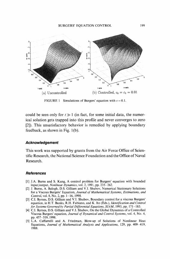
It is well known (see, e.g. [2,6]) that nonlinear problems, especiallyfluid dynamical problems, require extremely careful numerical analy-sis. Typically there is a trade-off between convergence, accuracy andnumerical oscillation. This is the case in particular when the initialdata is large relative to the viscosity coefficient e in Burgers’ equation.Higher order methods are preferred to lower order methods only whenthe time and/or spatial step sizes are sufficiently small, where the small-ness is a delicate question. It is not the purpose of our paper to find thebest approximation scheme for our problem, simply to demonstrateour theoretical results. Our numerical simulation is based on an uncon-ditionally stable, fully implicit scheme of second order accuracy, usingthree time level quadratic approximation in time and central differencescheme in space. The simulations were carried out on various plat-forms using several different numerical packages (OCTAVE, SCILAB,MATLAB), and they show grid independence for sufficiently smalltime and spatial grid.We consider first Burgers’ equation (2.1) with zero Neumann bound-

ary condition (uncontrolled system) and then the regulation errorsystem (2.4)-(2.7) with e 0.1 and with initial data Wo(X) Wo(x) Wa,where Wa= 3 and W0(x)= 20(0.5- x)3. The uncontrolled system isshown in Fig. l(a). The solution seems to converge to a nonzero"equilibrium" profile, although it eventually approaches zero, which


-3,i

"....’i.

0.6

0.4 "0.4

1 0.8

t-iS X-S

(a) Uncontrolled

0.6 ?"’.’0,4" 0.2

0.8

t-axis x-axis

(b) Controlled, co cl 0.01

FIGURE Simulations of Burgers’ equation with e--0.1.

could be seen only for >> (in fact, for some initial data, the numer-ical solution gets trapped into this profile and never converges to zero

[2]). This unsatisfactory behavior is remedied by applying boundaryfeedback, as shown in Fig. (b).

Acknowledgement

This work was supported by grants from the Air Force Office of Scien-tific Research, the National Science Foundation and the Office ofNavalResearch.

References

[1] J.A. Burns and S. Kang, A control problem for Burgers’ equation with boundedinput/output, Nonlinear Dynamics, vol. 2, 1991, pp. 235-262.

[2] J. Burns, A. Balogh, D.S. Gilliam and V.I. Shubov, Numerical Stationary Solutionsfor a Viscous Burgers’ Equation, Journal ofMathematical Systems, Estimations, andControl, vol. 8, No. 2, pp. 1-16, 1998.

[3] C.I. Byrnes, D.S. Gilliam and V.I. Shubov, Boundary control for a viscous Burgers’equation, in H.T. Banks, R.H. Fabiano, and K. Ito (Eds.), Identification and Controlfor Systems Governed by Partial Differential Equations, SLAM, 1993, pp. 171-185.

[4] C.I. Byrnes, D.S. Gilliam and V.I. Shubov, On the Global Dynamics of a ControlledViscous Burgers’ equation, Journal ofDynamical and Control Systems, vol. 4, No. 4,pp. 457-519, 1998.

[5] L.A. Caffarrelli and A. Friedman, Blow-up of Solutions of Nonlinear HeatEquations, Journal of Mathematical Analysis and Applications, 129, pp. 409-419,1988.


[6] J.H. Ferziger and M. Peri6, Computational Methods for Fluid Dynamics, Springer-Verlag, Berlin, 1996.

[7] V.A. Galaktionov and H.A. Levine, On Critical Fujita Exponents for HeatEquations with Nonlinear Flux Conditions on the Boundary, Israel Journal ofMathematics, 94, pp. 125-146, 1996.

[8] K. Ito and Y. Yan, Viscous Scalar Conservation Law with Nonlinear FluxFeedback and Global Attractors, Journal of Mathematical Analysis and Applica-tions, 227, pp. 271-299, 1998.

[9] M. Krsti6, On Global Stabilization of Burgers’ Equation by Boundary Control,Proceedings ofthe 1998 IEEE Conference on Decision and Control, Tampa, Florida.

[10] O.A. Ladyzhenskaya, V.A. Solonnikov and N.N. Ural’ceva, Linear and Quasi-linear Equations of Parabolic Type, Translations ofAMS, Vol. 23, 1968.

[11] H.A. Levine, Stability and Instability for Solutions of Burgers’ Equation with aSemi-linear Boundary Condition, SIAM Journal ofMathematical Analysis, vol. 19,No. 2, pp. 312-336, March 1988.

[12] H.V. Ly, K.D. Mease and E.S. Titi, Distributed and boundary control of theviscous Burgers’ equation, Numerical Functional Analysis and Optimization, vol. 18,pp. 143-188, 1997.

burgers’ equation with nonlinear boundary …flyingv.ucsd.edu/papers/pdf/40.pdfiiw(t)ll _<...

Documents