bulletin of the seismological society of america, vol. 70, no. … ray theory... · bulletin of the...

Bulletin of the Seismological Society of America, Vol. 70, No. 6, pp. 2021-2035, December 1980

ASYMPTOTIC RAY THEORY AND SYNTHETIC SEISMOGRAMS FOR LATERALLY VARYING STRUCTURES: THEORY AND APPLICATION TO

THE IMPERIAL VALLEY, CALIFORNIA

BY GEORGE A. MCMECHAN* AND WALTER D. MOONEY

ABSTRACT

The interpretation of refraction profiles that traverse laterally varying velocity structures has been hindered by lack of a practical algorithm for computing synthetic seismograms to compare with observations. However, a modification of zero-order asymptotic ray theory to incorporate the amplitudes of rays that turn in a velocity gradient, as well as reflected waves, allows the computation of high-frequency synthetic seismograms for laterally varying velocity structures. The method is general in that synthetic seismograms may be computed for any structure through which rays can be traced.

We have modeled seismic refraction data from the Imperial Valley, California, by applying this method. A major feature of our model is a sedimentary column that thickens from - 4 km at the Salton Sea to - 5 . 5 km at the United States- Mexico border. To approximate the observed amplitude behavior, a dipping velocity discontinuity was modeled near 13-km depth, but velocity gradients were found to be more appropriate than sharp boundaries in the rest of the model.

INTRODUCTION

Most presently available methods of constructing synthetic seismograms are invalid for laterally varying velocity structures. By contrast, detailed refraction and reflection data clearly indicate that lateral velocity variations are nearly universal. We here present a method of calculating synthetic seismograms for refracted and reflected waves in realistic Earth structures.

Asymptotic ray theory (cf. Cerven:~ et al., 1977; Cerven~, 1979b) is one method that has been shown to be valid for laterally varying structures. The method presented here is a modification of asymptotic ray theory as it is commonly used, and our study is, to our knowledge, the first attempt to apply it to the interpretation of refraction data.

THE ALGORITHM

Most currently used algorithms for computating synthetic seismograms are valid only for laterally homogeneous media. These algorithms include, among others, reflectivity (cf. Fuchs and Miiller, 1971), generalized ray expansions (cf. Wiggins and Helmberger, 1974), the full wave solution (cf. Richards, 1973), and various approximate methods (cf. Chapman, 1978).

Recently, Frazer and Phinney (1980) have generalized the phase integral method (Richards, 1973) for application to laterally inhomogeneous media and Hong and Helmberger (1978) presented examples of glorified optics synthetic seismograms computed for multiple reflections in some simple models with nonplanar boundaries. In this report we consider another option, asymptotic ray theory (ART). While ART is only approximate and has a number of restrictions, it is the only other method presently available that can compete in the study of body-wave propagation

* Permanent address: Pacific Geoscience Centre, P.O. Box 6000, Sidney, B.C., V8L 4B2, Canada.

2021

2022 GEORGE A. MCMECHAN AND WALTER D. MOONEY

in laterally varying media. Finite-difference and finite-element formulations can also be used but are rather expensive for routine modeling. For the modeling of strictly vertically inhomogeneous media, ART cannot compete in accuracy with the other methods mentioned above, but such models frequently do not adequately represent regions of complicated structure in the Earth, particularly in crustal studies.

Because the principles and limitations of ART are well known, only a superficial discussion of them is relevant here. Interested readers are referred to such texts as Cerven:~ and Ravindra (1971) and Cerven:~ et al. (1977) for details.

Because our interest is primarily in short-period seismograms, we consider zero- order ART to be an adequate approximation for most practical applications. One group of arrivals that originate in the higher order terms are head waves. In inhomogeneous media with curved interfaces, pure head waves rarely exist (Cerven:~ et al., 1977), and so the use of a zero-order application is not a severe limitation. This exclusion of head waves has the fortuitous advantage that the infinite amplitudes predicted by classical ART for head waves at critical points are no longer a difficulty. The approximation of head waves with turning rays is discussed below.

The zero-order ART algorithm can be simply expressed by (May and Hron, 1978)

where

A T = A o L -1 1-IKj ]

A T = the total complex amplitude associated with a ray; Ao = the initial amplitude; L = the geometrical spreading; and, II = the serial product over all the j complex plane-wave transmission and

reflection coefficients (K) along the ray path.

The construction of a synthetic arrival is implemented by performing a ray trace along which travel time, epicentral distance, and I-[K are accumulated. For ray tracing we employ an unpublished though widely used flat-earth Runga-Kutta integration code [(~erven:~ et al. (1977)]. Relatively complicated models can be handled by this program; the positions of curved interfaces and velocity discontinuities are defined by piecewise cubic splines, and lateral as well as vertical velocity gradients are possible. At the recording point, L is computed, AT is resolved into the desired component (vertical or radial), a surface conversion coefficient is computed if required, the phase is shifted by n~r/2 (where n is the number of internal caustics the ray has touched), and a time wavelet is constructed by a linear combination of a unit impulse with its Hilbert transform (cf. Cerven:~ and Ravindra, 1971). To generate a seismogram for a particular distance, a summation is performed over all the arrivals at that distance. Convolving with an appropriate apparent source function completes the seismogram.

The geometrical spreading, L, is determined by the algorithm described by Wesson (1970). The essence of this algorithm is contained in the expression

I Io - l = sin fi ~ " -~a 5 " ~ - ~ " Off ] J

where Io = the initial intensity associated with a unit solid angle; I = the intensity associated with an element of area of the wave front;

S Y N T H E T I C S E IS M OGR AM S FOR L A T E R A L L Y VARYING S T R U C T U R E S 2 0 2 3

07 = a vector joining points of equal travel time on adjacent rays; = the ray take-off angle measured from horizontal; and,

fi = the ray take-off angle measured from vertical.

This equation is valid for any three-dimensional medium through which rays can be traced; e.g., Daley and Hron (1979) used it for transversely isotropic media. We utilize it for two-dimensional media by computing both in-plane and out-of-plane spreading, assuming lateral homogeneity in the direction normal to the two-dimensional section. Implementation can be geometrically interpreted as the computation of the area of an element of the wave-front surface by determining the distances between points of equal travel time on adjacent rays. This algorithm does not resolve the problem of infinite amplitudes predicted for caustics (where the area of the ray tube goes to zero) but is stable elsewhere; e.g., it does not introduce false caustics that plague certain other algorithms (Wesson, 1970).

One method of calculating the response of a velocity gradient in a model is to approximate the gradient by a stack of thin homogeneous layers. The thin-layer approximation, previously used in generalized ray theory (Wiggins and Helmberger, 1974), has been described and applied in an ART context by Cerven) et al. (1977). Specifically, the amplitude of the critical reflection (the major contribution) associated with a thin layer is roughly proportional to the velocity contrast at the base of that layer (Wiggins and Helmberger, 1974). Because the net amplitude results from the constructive interference of adjacent contributions, the actual layer thicknesses chosen do not significantly alter the total amplitude, provided that these layers are sufficiently thin (cf. Ewing et al., 1957). In the high-frequency limit, this stationarity of amplitude can be employed directly without formally constructing thin layers, by treating the velocity gradient as in WKBJ approximation (Chapman, 1978). In zero-order amplitude computations for rays that traverse a velocity gradient, no transmission losses occur. The velocity contrast at the ray bottoming point in a velocity gradient is zero, and consequently, no energy is converted and no head wave is generated. Thus, the ray amplitude is not altered by passing through the turning point, a result consistent with the treatment of turning rays by Dey- Sarkar and Chapman (1978). This is the method we have used here.

To simulate a head wave as generated by other methods, we would have only to insert a small velocity gradient directly beneath the layer boundaries. Thus, in modeling "head" waves, a model derived using the present turning-ray approach would differ only slightly from that derived using an algorithm that specifically computes true head waves. As shown below, the discrepancies between synthetics generated by different methods are much smaller than the perturbations to the seismograms caused by lateral heterogeneities.

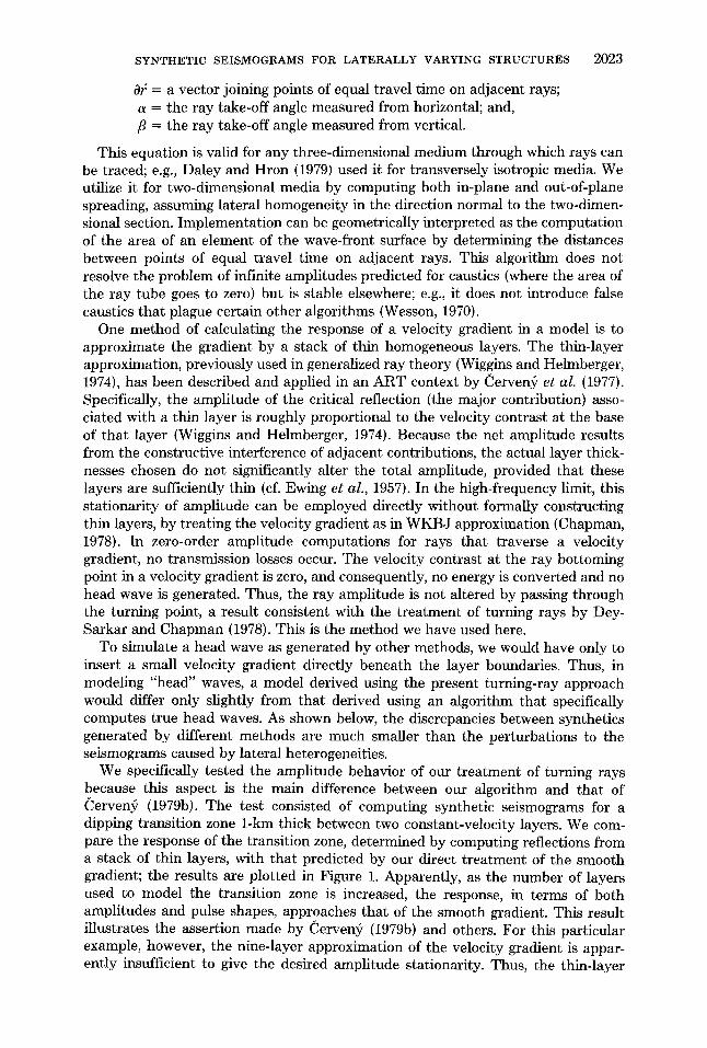
We specifically tested the amplitude behavior of our treatment of turning rays because this aspect is the main difference between our algorithm and that of Cerven~ (1979b). The test consisted of computing synthetic seismograms for a dipping transition zone 1-km thick between two constant-velocity layers. We compare the response of the transition zone, determined by computing reflections from a stack of thin layers, with that predicted by our direct treatment of the smooth gradient; the results are plotted in Figure 1. Apparently, as the number of layers used to model the transition zone is increased, the response, in terms of both amplitudes and pulse shapes, approaches that of the smooth gradient. This result illustrates the assertion made by Cerven:~ (1979b) and others. For this particular example, however, the nine-layer approximation of the velocity gradient is apparently insufficient to give the desired amplitude stationarity. Thus, the thin-layer


approximation is a relatively costly way to compute the response of a smooth velocity gradient: the computations for the nine-layer approximation were two orders of magnitude more expensive than those for the turning-ray approximation.

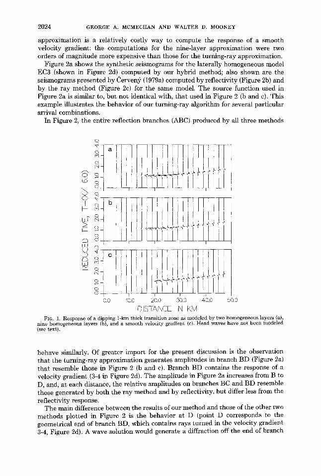
Figure 2a shows the synthetic seismograms for the laterally homogeneous model EC3 (shown in Figure 2d) computed by our hybrid method; also shown are the seismograms presented by Cerven~ (1979a) computed by reflectivity (Figure 2b) and by the ray method (Figure 2c) for the same model. The source function used in Figure 2a is similar to, but not identical with, that used in Figure 2 (b and c). This example illustrates the behavior of our turning-ray algorithm for several particular arrival combinations.

In Figure 2, the entire reflection branches (ABC) produced by all three methods

q

q Cq

O

@

x q

N O ~ ~

W o

U

C )

O <5

0.0 10.0 20,0 30,0 4-0.0 50.0

D ISTANC£ N KM FIG. 1. Response of a dipping 1-km thick transit ion zone as modeled by two homogeneous layers (a),

nine homogeneous layers (b), and a smooth velocity gradient (c). Head waves have not been modeled (see text).

behave similarly. Of greater import for the present discussion is the observation that the turning-ray approximation generates amplitudes in branch BD (Figure 2a) that resemble those in Figure 2 (b and c). Branch BD contains the response of a velocity gradient (3-4 in Figure 2d). The amplitude in Figure 2a increases from B to D, and, at each distance, the relative amplitudes on branches BC and BD resemble those generated by both the ray method and by reflectivity, but differ less from the reflectivity response.

The main difference between the results of our method and those of the other two methods plotted in Figure 2 is the behavior at D (point D corresponds to the geometrical end of branch BD, which contains rays turned in the velocity gradient 3-4, Figure 2d). A wave solution would generate a diffraction off the end of branch

S Y N T H E T I C S E I S M O G R A M S F O R L A T E R A L L Y V A R Y I N G S T R U C T U R E S 2025

BD. The ampli tude behavior of this diffraction is mimicked by the superposit ion of postcritical reflections and head waves in Figure 2 (b and c) (cfi Cerven:~ et al., 1977), but has no counterpar t in our algorithm. The introduction of a slight velocity gradient in the region 4-5 (Figure 2d) would allow turning rays to closely reproduce the behavior of the reflectivity and ray methods with only a minor per turbat ion to the velocity model. This point, which is similar to tha t made above in discussing head waves, means tha t the me thod used to generate synthetic seismograms affects the in terpreta t ion of data. Thus, differing modes of propagation used to model

X i

o

7 - Ai

I i 5-j

3 - !

1 -

a -1

7

-1

7

-1

I IIiIt, 10

E _~ 20 v ¢-

~ 3 0 "o

40

50

velocit, 5 6

0 ,

2'

model EC3

(km.s-1) 8 9

d

-3

0 50 100 150 200 250 3 0 0

distance (km)

FIG, 2. Response of the laterally homogeneous model EC3 (panel d) as computed by our turning-ray approximation (a), reflectivity (b), and the ray method (c). Panels (b) and (c) are reproduced from Cerven~ (1979a). Amplitude scaling in all three profiles is proportional to distance. The apparent source function used in (a) differs slightly from those used in (b) and (c). In (a), branch BD is the response of the gradient 3-4 (panel d) computed by turning rays (see text); in (b) and (c), it is computed by a summation of thin-layer responses. Branch AB is the subcritical reflection from discontinuity 2-3, B is the critical point, and branch BC is the postcritical reflection.

certain observed arrivals can lead to slight variations in the resulting velocity model. However, because amplitudes are part icularly sensitive to velocity gradients, only the finest s tructural details are influenced by the choice of modeling algorithm.

As an additional check on the overall ampli tude behavior of our algorithm, we computed synthet ic seismograms for the H I L D E R S model (Figure 3a) which has previously been used as a basis of comparison for different synthetic seismogram techniques (cf. Fuchs and Mfiller, 1971, Figure 8; Cerven:~ et al., 1977, Figure 4.13).


Our seismograms for the HILDERS model (Figure 3b) differ only in minor details from those generated by other algorithms that require homogeneous flat-layer models.

An example of the response of a more realistic model (Figure 4a) is plotted in Figure 4b. This model is composed entirely of velocity gradients (lateral as well as vertical), and so the seismograms consist entirely of refracted (turned) rays. Note the phase changes on the arrival branches corresponding to free-surface multiples (PP, PPP, and PPPP).

In an inhomogeneous medium (e.g., a velocity gradient), reflection coefficients are frequency dependent and thus must be computed via an energy algorithm when finite frequencies are considered (cf. Richards, 1973). However, for present purposes, because we have used zero-order ART (an infinite-frequency approximation), we can, within our assumptions, validly use plane-wave displacement coefficients. This point is important when finite-frequency algorithms are being coded [e.g., the phase

SYNTHETIC SE ISMOGRAMS

0 r<

0 \ r - - > < o

~-o ,/S-

Ld~

0 dZb c'i LLJ

LLI £Z:

v e l o c i t y ( k m . s -~ ) 4 6 8

0 J I i I i ~

1 2 O

0 . H I L D E R S

4 0

; t 70.0 90,0 110,0 130.0 150.0 170.0 30,0

D ISTANCE IN KM FIG. 3. Synthetic seismograms for the HILDERS model. The synthetic traces (b) were computed by

the modified ART method for the velocity-depth model (a).

integral method for laterally varying media, presented by Fraser and Phinney (1980)].

The ART approach can be used to model P waves, S waves, converted phases, multiples, internal reflections, and head waves. At present we have included only P waves, their multiples, and internal reflections. Precritical reflections are generated, but diffractions beyond caustics and in shadow zones are not because these are wave phenomena and thus are not given by a ray solution. The source, a unit impulse in displacement, may be placed anywhere in the model; for nonsurface sources, rays leaving the source upward as well as downward are included. Convolution of the impulse response with a realistic time source function aids in modeling observations where successive arrivals interfere with each other.

An additional option which may be incorporated into the ART formulation is the inclusion of various source radiations of increased complexity (e.g., a double couple for earthquake sources) although this is not required for the shot-profile interpre-

SYNTHETIC SEISMOGRAMS FOR LATERALLY VARYING STRUCTURES 2027

ta t ions presented below. Anelastic a t t enua t ion m a y also be included; Smi th (1977) computed a t t enua t ion in an A R T context using the a lgori thm of F u t t e r m a n (1962).

DATA

We have modeled seismic refract ion da ta f rom the Imper ia l Valley, California (Fuis et al., 1980), by applying the A R T m e t hod described above. The model consists of an isotropic but la teral ly varying two-dimensional medium.

The da ta chosen for this s tudy are f rom a reversed profile be tween shot points 06 and 13 (Figure 5). This profile was selected for detailed in terpre ta t ion because it provides, by vir tue of its location and length, the best available informat ion con-

Z

i

[3_ k~

DISTANCE ~ KM 0.0 5.0 10.0 15.0 20.0 25~] 30.0 ~5.0 40.0

o i. i ~ i ~ ~ J -4 d i ~°° ~'~ ~ ~ ~' ~ ~'

Q

~o o

x Y q k ©

~ Q C5 (N

© u

0o0 40 10.0 15.0 20.0 25.0 30.0 35.0

DiSTANCE JN k<k4 FIG. 4. The response of a model (a) derived from a detailed reversed seismic refraction profile in the

Imperial Valley, California (Fuis et al., 1980) is shown in (b). The model has no first-order discontinuities. The numbers placed along the boundaries in (a) indicate the velocity both above and below the boundary at those points (except for the free-surface boundary, where the velocity is that of air above the boundary). The velocity at any particular point in the model is calculated by interpolation (cf. Cerven~ et al., 1977, section 3.7.1). The arrival branches labeled PP, PPP, and PPPP are free-surface multiples. The shot point for the computation of the synthetic seismograms is indicated by the triangle in (a). Distances in (b) are from the shot point. The apparent source wavelet is a slightly smoothed unit impulse.

cerning the veloci ty-depth s t ructure of the central Imper ia l Valley. Each of the two profiles was recorded by 100 identical ins t ruments f rom a single shot; this procedure aids in correlat ing arrivals across the profiles. T h e recording sites were identical for bo th shots. All records are vertical components . The total n u m b e r of records available for profile 13-06 is 79, of which 62 are displayed in Figure 6. The total n u m b e r of records available for profile 06-13 is 83, of which 65 are displayed in Figure 7. Where two records would overlap on these plots, only the record with the highest signal-to-noise rat io was plotted.

In addit ion to clear first arrivals, the profiles (Figures 6 and 7) are character ized by p rominen t secondary arrivals tha t include subsurface reflections and free-surface

2028 G E O R G E A. M C M E C H A N A N D W A L T E R D. M O O N E Y

multiples. Modeling of these secondary arrivals is an impor tant aspect of our analysis and has significantly constrained the model beyond tha t possible from analysis of first arrivals alone.

Profile 13-06 (Figure 6) runs from the west side of the Salton Sea southeastward to the Uni ted States-Mexico border (Figure 5). On this profile, the smooth curve (AB, Figure 6) for first arrivals between 3 and 14 km, indicates a velocity continu- ously increasing with depth in the sedimentary column. Between 15 and 55 km, the first arrivals, which are refractions in the basement, form a relatively straight line (branch BC) with an apparent velocity of 5.55 km/sec. Beyond 55 km, the first

33 40 33 40 IMPERIAL VALLEY SEISMIC REFRACTION SURVEY, 19"79

• RECORDER LOCATIONS FOR 1979 SURVEY

• ,~. 8HOTPOINTS 18 & 6 ~ • •~ • OTHER 8HOTPOINT8

• ~!ii~ii: . • =~, ~iiz]/[~;~i~ AR~A OF PRESENT INVESTIGATION

~4

•

• • . . . . . . . . . . . ! 3 3 0 5

X ,13

S A L T O N S E A

--=.

'~, "" '!iiiiHiii • . t . .EL cE, , ,o •.

_cA LL,~-. t . . . . . . . 4 " " ~ ' = M E X I C O

A t

S.AW'EY : 2L " , J

• • • • • 0 I 0 20 / ~ A A • • • • I ~ (

'=' • k m N

!iiiiiiiii~ A= • • •

~/'~ J

32 30 32 30

FIG. 5. Location map for the Imperial Valley seismic refraction experiment of 1979. Only the reversed profffles between shot points 06 and 13 are considered in this study. The large "X" west of shot point 13 indicates the bottoming point of a prominent crustal reflector identified by Hamilton (1970). This reflector is also identifiable in the present study.

arrivals are a subbasement refract ion (DE) with an apparent velocity of 7.7 km/sec. A triplication (BCDE) evident beyond 40 km indicates a high-velocity gradient in the region of t ransi t ion from basement to subbasement. This triplication is consistent ly observed in Imperial Valley profiles tha t extend to sufficient distances (cf. Hamilton, 1970; Fuis et al., 1980).

The travel- t ime curves of free-surface multiples (branch AF for the P P arrivals and branch AH for the P P P arrivals, Figure 6) are observed, as expected, to be "s t re tched" in bo th t ime and distance relative to the first-arrival curve by an amount proport ional to their multiplicity (2 and 3, respectively).

S Y N T H E T I C S E I S M O G R A M S F O R L A T E R A L L Y V A R Y I N G S T R U C T U R E S 2029

Profile 06-13 (Figure 7) runs to the nor thwes tward f rom the internat ional border to the west side of the Salton Sea (Figure 5); the major features of this profile resemble those of profile 13-06. Proceeding outward f rom the shot point, the first arrivals again smooth ly approach the basemen t velocity (branch AB, Figure 7), a tr iplication (BCDE) occurs, a higher subbasemen t velocity is evident (branch DE), and free-surface mult iples are present (branches AF and AH).

Significant differences, however, exist be tween profiles 13-06 and 06-13. In profile

(a)

: 0

8 C22

SE

F

E

(b) ' ~

F

e

PF

NW

T-

80.0 70.0 60.0 50.0 4-0.0 .30.0 20.0 I0.0 0.0

D ISTANCE IN KM FIG. 6. Observed (a) and synthetic (b) record sections for profile 13-06. The apparent source function

used in the synthetics is shown in the inset to (b). Specific refraction and reflection branches discussed in the text are similarly labeled by letters A through G on both profiles. The dashed lines on the observed profile (a) correspond to the theoretical arrival times in the synthetic profile (b). The wave groups labeled P P and P P P are free-surface multiples. Each synthetic trace is scaled by a factor proportional to the square root of its distance. The observed traces are plotted such that each has approximately the same maximum amplitude; no attempt was made to recover true amplitudes.

06-13, the t ravel t imes indicate a higher near-surface velocity t han in profile 13-06, a l though similar velocity gradients are present . T h e appa ren t velocity of the base- m e n t refract ion in profile 06-13 is ~5.95 km/sec , a velocity -0 .4 k m / s e c higher than tha t observed in profile 13-06. The appa ren t velocity of the subbasemen t refract ion in profile 06-13 is -7 .1 km/sec , a velocity ~0.6 k m / s e c lower than tha t in profile 13- 06. T h e p rominen t tr ipl ication (BCDE, Figure 7) contains a high ampl i tude cusp a t ~30 k m in profile 06-13 in contras t to tha t a t ~40 k m in profile 13-06.


All major features of these two profiles, including their dissimilarities as well as similarities, can be modeled by a two-dimensional (laterally as well as vertically varying) structure composed essentially of dipping, nonhomogeneous layers separated by transition zones.

~NTERPRETATION

In this section, we summarize the procedure used to model the data described above; each major feature of the model is considered in turn from the surface

>o ill ,_., ,s :Y t5

ill cq- ' q

f22

W

~ Q LL] Cq-

t ~ ( d [2:

(a)

iiitl jill tt l ll ?;il l ltt; tliIiI ltl!t ltliIl t

( b ) -

30.0 4.0.0

SE

0.0 10.0 20.0

IIW

t G

50.0 60,0 70.0 80.0

D ISTANCE IN KM FIG. 7. Comparison of observed (a) and synthetic (b) record sections for profile 06-13. Figure labeling

and amplitude scaling are the same as in Figure 6. A particularly clear amplitude effect of lateral variation is seen by comparing cusp D here with that in Figure 6. The apparent source function used in (b) is not the same as in Figure 6b. An apparent source function contains an approximation to the true source function, interaction with the free surface, near-shot and near-receiver structure, and the instrument response. The apparent source functions were defined by extracting an average wavelet from the P branch at distances at which it appears to be free from interference with other branches (15 to 30 km).

downward. To maximize the amount of velocity information extracted from the data profiles, we consider the observed amplitude behavior as well as the travel times. Amplitudes are particularly sensitive to velocity gradients and discontinuities; inclusion of amplitude constraints is implemented by the computation of synthetic seismograms that can be compared with the observed profiles.

The application of the amplitude constraints is, to some degree, subjective because true amplitude record sections were unavailable. Although compaTison of amplitudes

S Y N T H E T I C S E I S M O G R A M S F O R L A T E R A L L Y V A R Y I N G S T R U C T U R E S 2 0 3 1

on adjacent traces is not strictly valid, the relative ampli tudes of success ive arrivals in each recorded trace are correct. We have therefore tried to reproduce the averaged behavior of each arrival branch as a funct ion of distance on the basis of the observed changes in intratrace relative ampli tudes with distance. A comparison of ampli tude ratios f o r several representat ive arrival pairs on both observed and synthet ic se i smograms is presented in Figure 9. M a n y local ampli tude fluctuations, especial ly on the mult iple branches, are due to focusing and defocusing by local ve loci ty variations that we have not a t tempted to model . We concentrate on finding the s implest mode l that can explain the dominant ampli tude trends and features (the posi t ions of the main ampl i tude decrease in each of the P, PP, and P P P branches, and the critical reflections).

Our interpretation begins by fitting first-arrival travel t imes with straight l ines to

shot point

1 3

0

0 '2.20

5:.00

4 ~.65

E 8 ,,r

I-.--12

16

2 0

shot po in t

6

distance (km) ~ -~ 1 0 2 0 3 0 4 0 5 0 6 0 7 0 8 0

0 12.00 I 1"80 I 1.801 '1.~0 ' 1. ]0 ' 1.80

5,00 5.00 5.05 5.10 5.10 5.10" 4

5.6:

o 8

5.85

7.2C 12

( k m ) 0 5 1 0

" ' 0 ~, ~

: 2 0 ~ --

a c ~ 1

L ~ ~

P - w a v e v e l o c i t y

2 3 4 5 ! ! ! 1

15

o o

( k m . s -1 }

6 7 0 !

4

8-g

t2~

16

2 O

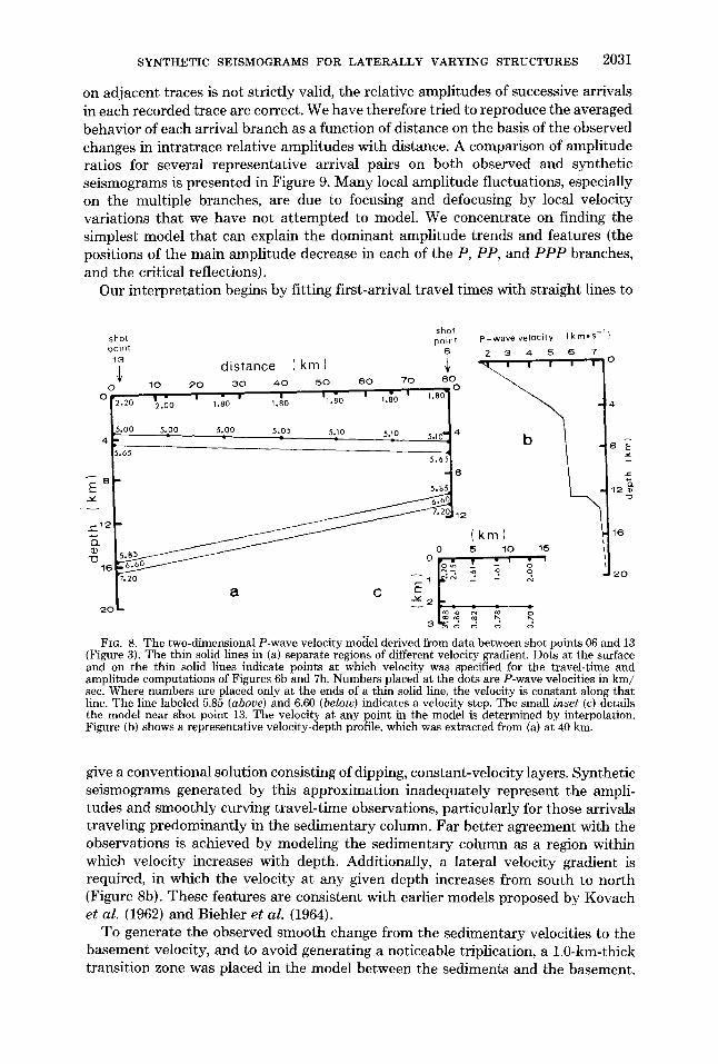
Fro. 8. The two-dimensional P-wave velocity moc[el derived from data between shot points 06 and 13 (Figure 3). The thin solid lines in (a) separate regions of different velocity gradient. Dots at the surface and on the thin solid lines indicate points at which velocity was specified for the travel-time and amplitude computations of Figures 6b and 7b. Numbers placed at the dots are P-wave velocities in km/ sec. Where numbers are placed only at the ends of a thin solid line, the velocity is constant along that line. The line labeled 5.85 (above) and 6.60 (below) indicates a velocity step. The small inset (c) details the model near shot point 13. The velocity at any point in the model is determined by interpolation. Figure (b) shows a representative velocity-depth profile, which was extracted from (a) at 40 km.

give a convent ional so lut ion consist ing of dipping, constant-ve loc i ty layers. Synthet ic se i smograms generated by this approximation inadequately represent the amplitudes and s m o o t h l y curving travel-t ime observations, particularly for those arrivals traveling predominant ly in the sedimentary column. Far better agreement with the observat ions is achieved by model ing the sedimentary co lumn as a region within which ve loc i ty increases with depth. Additionally, a lateral ve loci ty gradient is required, in which the veloci ty at any given depth increases from south to north (Figure 8b). T h e s e features are consis tent with earlier mode l s proposed by Kovach et al. (1962) and Biehler et al. (1964).

T o generate the observed s m o o t h change from the sedimentary velocit ies to the basement velocity, and to avoid generating a not iceable triplication, a 1.0-km-thick transit ion zone was placed in the mode l be tween the sediments and the basement .


The velocity increases from -5.1 km/sec at the top of the transition zone to 5.65 km/sec at the bottom.

In the basement beneath the transition zone, the velocity gradient is much lower than in either the transition zone or the overlying sediments. This change of gradient causes an abrupt drop in relative amplitude to -20-km distance in the first arrivals, at ~35 km in the PP branch, and at ~45 km in the PPP branch (Figures 6, 7, and 9). Differences between the two profiles in the precise position of these features are due to the southward dip of the transition zone (Figure 8a).

o_ 5

t 2 G. I

0 i r , i i i i i i i i i , i

I0 2 0 5 0 40 50 60 70 (kin

° h ]2 ca % ,. o ] k EL. c \ ~ : ~ E I G _

i i I I

0 t ~ " ~ - - 0

. . . . 5'0 ' 4'0 . . . . . . I0 20 I0 20 50 40 (km) (kin)

, 4

/ ', o13G_

c o P o \ - - / o"~, G_

Ot 20 30 40 L , i ~ I ' I I / i I i I

I0 20 50 40 50 (km)

£ :S- °o ".. :"."

20 50 40 50 ' ' ' ' J I i 2 1 0 I ' ', f f

I0 50 4O 5O (kin)

Fro. 9. Representative observed and calculated amplitude ratios as functions of distance. In each panel, the symbols are observed amplitude ratios for the arrival pairs indicated on the vertical axis, and the line {solid or dashed) is taken from the synthetic seismograms. Paaels (a) through (d) are for profile 06-13 and (e) through (g) are for profile 13-06. All amplitudes are peak-to-peak. In distance ranges where an arrival is multi-branched, the first-arrival amplitude was used except in (d), where Pr refers to the reflection branch.

The basement arrivals in both profiles were modeled by a velocity that increases linearly from 5.65 km/sec at the top to 5.85 km/sec at the bottom. Unlike the smooth sediment to basement transition, evidence (the prominent triplication BCDE, Figures 6 and 7) exists for a relatively abrupt velocity increase from -5.85 to -7.2 km/sec at a depth as shallow as 10 km. This triplication appears to be the same as that observed by Hamilton (1970) to the northwest of the present study area. The abrupt velocity increase was modeled in two parts; a step increase from 5.85 to 6.60 km/sec, and a 0.9-km-thick transition zone in which the velocity


increases smoothly from 6.6 to 7.2 km/sec (Figure 8b). This combination was chosen in order to place the critical reflections (point D, Figures 6 and 7) at their observed distances while including the large velocity increase required by the travel times of the arrivals refracted in the lower medium (branch DE, Figures 6 and 7). The relative amplitude of the critical reflection in profile 06-13 is larger than that in profile 13-06. This is reproduced by the model as a result of the northward dip of the lower transition zone (Figure 8a). The large "X" in the center left of Figure 5 indicates the approximate position of the bottoming point for the critical reflection observed by Hamilton (1970). This reflective boundary is therefore not confined to the Imperial Valley. In addition, the corresponding critical reflection in the PP branch is observed in profile 06-13 (near point G), but not in profile 13-06, because it is off the end of the recorded profile.

A segment of an arrival branch observed on profile 06-13 between branches DE

F~G. 10. Ray paths involved in the propagation of PP in a laterally inhomogeneous medium. Dashed lines represent a transition zone similar to tha t at ~4-km depth in Figure 8. Each ray shown represents a family of similar rays. Each family (a to e) contributes in turn to the PP branch at successively greater distances. In our velocity model (Figure 8), an abrupt decrease of amplitude is associated with the progression from family (c) to family (d) (cf. Figures 6 and 7). A similar progression is involved in the propagation of the P P P branch.

and DC beyond 65 km (indicated by the arrows on Figure 7a) has a high apparent velocity (8.22 km/sec). This segment may indicate the existence of a deeper layer; its high amplitude is consistent with a critical reflection, possibly from the moho. A flat-layer solution yields a depth of 22.9 km for this reflector, and the method of Giese (1976) gives a maximum depth of 28.7 km.

One particularly important aspect of our modeling has been the generation of the PP and PPP wave groups. Much of the energy propagating in these branches travels in asymmetric paths that would not exist in a laterally homogeneous, nondipping structure (Figure 10). High velocity gradients in both the sedimentary column and the sediment to basement transition combine to support the relatively energetic propagation of the PP and P P P branches to extended ranges as evident in Figures 6 and 7. The effect of a dipping structure is evident in comparing the energy distributions in these reversed profiles.


DISCUSSION

This study demonstrates the feasibility of synthetic seismogram modeling of refraction and reflection data in two-dimensional velocity structures. The technique is general in the sense that synthetics can be computed for any two-dimensional structure through which rays can be traced. Although several approximations are involved in our formulation, the resulting high-frequency seismograms compare favorably with those generated by other techniques. Indeed, the differences between synthetic profiles computed by diverse methods are small compared to the effects of lateral crustal velocity variations. Thus, an approximate method for generating synthetic seismograms for models of laterally varying media is of greater value in studying lateral changes than a more exact method that can deal only with vertically varying velocity.

We have performed a detailed travel-time and amplitude analysis of the major features of a reversed seismic profile to create a detailed velocity model for the central Imperial Valley. The major features of the model are a sedimentary column that thickens from the Salton Sea to the United States-Mexico border and a deep major intracrustal transition that dips from southeast to northwest (Figure 8). To approximate the observed amplitude behavior, we modeled a dipping velocity discontinuity at ~13-km depth and found velocity gradients to be more appropriate than sharp boundaries in the rest of the model. Our model differs from that for the uppermost crust presented by Kovach et al. (1962) and Biehler et al. (1964), which is composed of constant-velocity layers separated by sharp boundaries.

We cannot be precise regarding the resolution achieved by this method, but we find that changes of 0.1 km in the thicknesses of the transition zones significantly affect amplitudes. Travel times are generally fitted to +0.05 sec. Also, because the P P and P P P branches as well as first-arrival data were simultaneously modeled on both profiles, we had approximately 6 times as many constraints as would be available on a single unreversed profile. The least constrained aspect of the model is the velocity beneath the subbasement transition because only the uppermost part of this region was sampled by this experiment.

One factor not included here that may account for some of the local amplitude and frequency variations observed in the data is anelastic attenuation. The inclusion of attenuation probably would not alter the general features of the model presented here, but could aid in an investigation of detailed material properties. Since we have not considered finite frequencies, true amplitudes, or attenuation in this preliminary study, ample scope remains for future modeling of these data.

Certain aspects of our model contain tectonic implications. For example, the profile 06-13 appears to lie along or near the axis of the basement expression of the Salton trough; the opposite direction of dip of the basement and subbasement layers may indicate isostatic compensation; the existence of a high-velocity subbasement at shallow depth may constrain the nature of earthquake generation at various depths; and, the velocities themselves, which are not characteristic of either conti- nental or oceanic origin indicate a transitional structure. Consideration of these tectonic implications is beyond the scope of this report and is the subject of continuing investigations.

ACKNOWLEDGMENTS

This project was completed while one of the authors (G.A.M.) was on leave at the U.S. Geological Survey (USGS), Menlo Park, California, which provided a stimulating environment and computing facilities. Discussions with B. Angstman, P. Spudich, R. Nowack, G. Fuis, and W. Lutter were helpful at


various stages of the work. The data were collected by the USGS seismic refraction field crew under the expert guidance of J. Healy, G. Fnis, and D. Hill. Critical reviews by P. Spudich and D. Warren are much appreciated as is the patient typing of many drafts of this paper by R. Rebello. The project was supported in part by the Department of Energy, Mines and Resources, Canada, Earth Physics Branch, no. 869.

REFERENCES

Biehler, S., R. L. Kovach, and C. R. Allen (1964). Geophysical framework of the northern end of the Gulf of California structural province, in Marine Geology of the Gulf of California, T. Van Andel and G. Shor, Editors, AAPG Mere. 3, 126-143.

Cerven~, V. (1979a). Accuracy of ray theoretical seismograms, J. Geophys. 46, 135-149. Cerven:~, V. (1979b). Ray theoretical seismograms for laterally inhomogeneous structures, J. Geophys.

46, 335-342. (~erven:~, V. and R. Ravindra (1971). Theory of Seismic Head Waves, University of Toronto Press,

Toronto, 313 pp. (~erven~, V., I. A. Molotkov, and I. PgenSik (1977). Ray Method in Seismology, Univerzita Karlova,

Praha, 214 pp. Chapman, C. H. (1978). A new method for computing synthetic seismograms, Geophys J. 54, 481-518. Daley, P. F. and F. Hron (1979). SH waves in layered transversely isotropic media--An asymptotic

expansion approach, Bull. Seism. Soc. Am. 69, 689-711. Dey-Sarkar, S. K. and C. H. Chapman (1978). A simple method for the computation of body wave

seismograms, Bull. Seism. Soc. Am. 68, 1577-1593. Ewing, W. M., W. S. Jardetzky, and F. Press (1957). Elastic Waves in Layered Media, McGraw-Hill,

New York, 380 pp. Frazer, L. N. and R. A. Phinney {1980). The computation of finite frequency body wave synthetic

seismograms in inhomogeneous elastic media, preprint. Fuchs, K. and G. Mfiller (1971). Computation of synthetic seismograms with the reflectivity method and

comparison with observations, Geophys J. 23, 417-433. Fuis, G. S., W. D. Mooney, J. H. Healy, W. J. Lutter, and G. A. McMechan (1980). Crustal structure of

the Imperial Valley region, U.S. Geol. Surv. Profess. Paper (in press). Futterman, W. I. (1962). Dispersive body waves, J. Geophys. Res. 67, 5279-5291. Giese, P. (1976). Depth calculation in Explosion Seismology in Central Europe, P. Giese, C. Prodehl,

and A. Stein, Editors, Springer-Verlag, New York, 429 pp. Hamilton, R. M. (1970). Time-term analysis of explosion data from the vicinity of the Borrego Mountain,

California, earthquake of 9 April 1968, Bull. Seism. Soc. Am. 60, 367-381. Hong, T.-L and D. V. Helmberger (1978). Glorified optics and wave propagation in nonplanar structure,

Bull. Seism. Soc. Am. 68, 1313-1330. Kovach, R. L., C. K. Allen, and F. Press (1962). Geophysical investigations in the Colorado delta region,

J. Geophys. Res. 67, 2845-2871. May, B. T. and F. Hron (1978). Synthetic seismic sections of typical petroleum traps, Geophysics 43,

1119-1147. Richards, P. G. (1973). Calculation of body waves for caustics and tunnelling in core phases, Geophys. J.

35, 243-264. Smith, S. G. (1977). A reflection profile modelling system, Geophys. J. 49, 723-737. Wesson, R. L. (1970). A time integration method for computation of the intensities of seismic rays, Bull.

Seism. Soc. Am 60, 307-316. Wiggins, R. A. and D. V. Helmberger (1974). Synthetic seismogram computation by expansion in

generalized rays, Geophys J. 37, 73-90.

U.S. GEOLOGICAL SURVEY 345 MIDDLEFIELD ROAD MENLO PARK, CALIFORNIA 94025

Manuscript received March 13, 1980

bulletin of the seismological society of america, vol. 70, no. … ray theory... · bulletin of the...

Documents