building bridges between neural models

Diffusion Models of Decision Making 1

Building Bridges between Neural Models

and

Complex Decision Making Behavior

Jerome R. Busemeyer1

Ryan K. Jessup1

Joseph G. Johnson2

James T. Townsend1

March 21, 2006

1) Department of Psychological and Brain Sciences, Indiana University, Bloomington, IN,

USA

2) Department of Psychology, Miami University, Oxford, OH, USA

This work was supported by a National Institute of Mental Health Cognition and Perception

Grant MH068346 to the first author and a National Institute of Mental Health Grant 1 RO1

MH62150-01 to the second author.

Send Correspondence to: Jerome R. Busemeyer 1101 E. 10th St. Bloomington, Indiana, 47405 voice: 812 -855 – 4882 fax: (812) 855-4691 [email protected]

mailto:[email protected]


Building Bridges between Neural Models and Complex Decision Making Behavior

Diffusion processes, and their discrete time counterparts, random walk models, have

demonstrated an ability to account for a wide range of findings from behavioral decision

making for which the purely algebraic and deterministic models often used in economics and

psychology cannot account. Recent studies that record neural activations in non-human

primates during perceptual decision making tasks have revealed that neural firing rates

closely mimic the accumulation of preference theorized by behaviorally-derived diffusion

models of decision making.

This article bridges the expanse between the neurophysiological and behavioral

decision making literatures; specifically, decision field theory (Busemeyer & Townsend,

1993), a dynamic and stochastic random walk theory of decision making, is presented as a

model positioned between lower-level neural activation patterns and more complex notions

of decision making found in psychology and economics. Potential neural correlates of this

model are proposed, and relevant competing models are also addressed.

Keywords: Models, Dynamic; Choice Behavior; Decision Making; Basal Ganglia;

Neuroeconomics; Processes, Diffusion/Random Walk;


The decision processes of sensory-motor decisions are beginning to be fairly well

understood both at the behavioral and neural levels. For the past ten years, neuroscientists

have been using multiple cell recording techniques to examine spike activation patterns in

rhesus monkeys during simple decision making tasks (Britten, Shadlen, Newsome, &

Movshon, 1993). In a typical experiment, the monkeys are presented with a visual motion

detection task which requires them to make a saccadic eye movement to a location indicated

by a noisy visual display, and they are rewarded with juice for correct responses. Neural

activity is recorded from either the middle temporal area (an extrastriate visual area), lateral

intraparietal cortex (which plays a role in spatial attention), the frontal eye fields (FEF), or

superior colliculus (SC, regions involved in the planning and implementation of eye

movements, respectively).

The typical findings indicate that neural activation regarding stimulus movement

information is accumulated across time up to a threshold, and a behavioral response is made

as soon as the activation in the recorded area exceeds the threshold (see Schall, 2003; Gold &

Shadlen, 2000; Mazurek, Roitman, Ditterich, & Shadlen, 2003; Ratcliff, Cherian, &

Segraves, 2003; and Shadlen & Newsome, 2001, for examples). Because areas such as FEF

and SC are thought to implement the behavior of interest (in this example, saccadic eye

movements), a conclusion that one can draw from these results is that the neural areas

responsible for planning or carrying out certain actions are also responsible for deciding the

action to carry out, a decidedly embodied notion.

Mathematically, the spike activation pattern, as well as the choice and response time

distributions, can be well described by what are known as diffusion models (see Smith &

Ratcliff, 2004, for a summary). Diffusion models can be viewed as stochastic recurrent


neural network models, except that the dynamics are approximated by linear systems. The

linear approximation is important for maintaining a mathematically tractable analysis of

systems perturbed by noisy inputs. In addition to these neuroscience applications, diffusion

models (or their discrete time, random walk, analogues) have been used by cognitive

scientists to model performance in a variety of tasks ranging from sensory detection (Smith,

1995), and perceptual discrimination (Laming, 1968; Link & Heath, 1978; Usher &

McClelland, 2001), to memory recognition (Ratcliff, 1978), and categorization (Nosofsky &

Palmeri, 1997; Ashby, 2000). Thus, diffusion models provide the potential to form a

theoretical bridge between neural models of sensory-motor tasks and behavioral models of

complex-cognitive tasks.

The purpose of this article is to review applications of diffusion models to human

decision making under risk with conflicting objectives. Traditionally, the field of decision

making has been guided by algebraic utility theories such as the classic expected utility

model (von Neumann & Morgenstern, 1944) or more complex variants such as cumulative

prospect theory (Tversky & Kahneman, 1992). However, a number of paradoxical findings

have emerged in the field of human decision making that are difficult to explain by

traditional utility theories. We show that diffusion models provide a cogent explanation for

these complex and puzzling behaviors. First, we describe how diffusion models can be

applied to risky decisions with conflicting objectives; second, we explain some important

findings using this theory; and finally, we compare this theory with some alternate competing

neural network models.


1. Risky Decisions with Multiple Objectives

Consider the following type of risky decision with multiple objectives. Suppose a

commander is suddenly confronted by an emergency situation, and must quickly choose one

action from a set of J actions, labeled here as A1, …, Aj ,…, AJ. The payoff for each action

depends on one of set of K uncertain states of the world X1, …, Xk, ,…, XK. The payoff

produced by taking action j under state of the world k is denoted xjk Finally, each payoff can

be described in terms of multiple competing objectives (e.g., one objective is to achieve the

commander’s mission while another objective is to preserve the commander’s resources).

According to the ‘rational’ model (von Neumann & Morgenstern, 1944; Savage,

1954), the decision maker should choose the course of action that maximizes expected utility:

EU(Aj) = Σk pk ⋅ u(xjk), where pk is the probability of state Xk and u(xjk) is the utility of payoff

xjk. Psychological variants of expected utility theory modify the classic model by replacing

the objective probabilities with subjective decision weights (e.g., Tversky & Kahneman,

1992; Birnbaum, Coffey, Mellers, & Weiss, 1992).

2. Decision Field Theory

An alternate approach towards explaining risky choice behavior involves the

application of diffusion processes, via decision field theory. We have applied diffusion

models to a broad range of results including findings from decision making under uncertainty

(Busemeyer & Townsend, 1993), multi-attribute decisions (Diederich, 1997), multi-

alternative choices (Roe, Busemeyer, & Townsend, 2001) and multiple measures of

preference (Johnson & Busemeyer, 2005). The basic assumptions of the model are

summarized below.


2.1 Basic Assumptions.

Define P(t) as a J dimensional preference state vector, and each coordinate, Pj(t),

represents the preference state for one of the J actions under consideration. The preference

states may range from positive (approach states) to negative (avoidance states), and the

magnitude of a preference state represents the strength of the approach-avoidance tendency.

The initial state at the beginning of the decision process, P(0), represents preferences before

any information about the actions is considered, such as memory from previous experience

with a decision problem (∑j Pj(0) = 0). For novel decisions, the initial states are all set equal

to zero (neutral), Pj(0) = 0 for all j. The change in state across a small time increment h is

denoted by dP(t) = P(t) – P(t-h).

During deliberation the preference state vector evolves according to the following

linear stochastic difference equation (t = n⋅h and n = 1, 2, …)

dP(t) = –h⋅Γ⋅P(t−h ) + V(t) (1a)

or equivalently

P(t) = (I–h⋅Γ) ⋅P(t−h ) + V(t) = S⋅P(t−h ) + V(t) (1b)

where S = (I–h⋅Γ) is a J × J feedback matrix, V(t) is a J dimensional stochastic input, and I is

the identity matrix. The solution to this linear stochastic difference equation equals

P(t) = . (2) ∑−

=

+−1

0

)0()(n

n PhtVτ

τ τ SS

As h 0, this system approximates an Ornstein - Uhlenbeck diffusion process (see

Busemeyer & Townsend, 1992; Busemeyer & Diederich, 2002). If the feedback matrix is set

to S = I (i.e. Γ = 0), then the Ornstein-Uhlenbeck model reduces to a Wiener diffusion

process.


The feedback matrix Γ contains self feedback coefficients, γii = γ are all equal across

the diagonals, as well as symmetrical lateral inhibitory connections γij = γji. The magnitudes

of the lateral inhibitory connections are assumed to be inversely related to the conceptual

distance between the actions (examples are discussed later). The preference state vector,

P(t), remains bounded as long as the eigenvalues of S are less than one in magnitude. Lateral

inhibition is commonly used in competitive neural network systems (Grossberg, 1988;

Rumelhart & McClelland, 1986).

The stochastic input vector, V(t), is called the valence, and each coordinate, Vj(t),

represents avoidance (when activations are negative) or approach (when activations are

positive) forces on the preference state for the jth action. The valence vector is decomposed

into three parts as follows:

V(t) = C⋅M⋅W(t), (3)

where C is a J × J contrast matrix, M is a J × K value matrix, and W(t) is a K × 1 stochastic

attention weight vector. Each element, mjk, of the value matrix M represents the affective

evaluation of each possible consequence k for each action j. The product of the stochastic

attention weight vector with the value matrix, M⋅W(t), produces a weighted average

evaluation for each action at any particular moment. The contrast matrix C has elements cij =

1 for i = j and cij = -1/(J-1) for i ≠ j, which are designed to compute the advantage or

disadvantage of each action relative to the average of the other actions at each moment. (Note

that ∑ j cij = 0 implies that ∑ Vj(t) = 0.)

The weight vector, W(t) , is assumed to fluctuate from moment to moment,

representing changes in attention to the uncertain states across time. More formally, the

attention weights are assumed to vary according to a stationary stochastic process with mean


E[W(t)] = w⋅h, and variance-covariance matrix Cov[W(t)] = Ψ⋅h.1 The mean weight vector,

w, is a K × 1 vector, and each coordinate, wk = E[Wk(t)], represents the average proportion of

time spent attending to a particular state, Xk , with k ∈ 1, …, K.

2.2 Derivations

These assumptions lead to the following implications. The mean input valence equals

E[V(t)] = δ⋅h = (C⋅M⋅w)⋅h, and the variance-covariance matrix of the input valence equals

Cov[V(t)] = Φ⋅h = (CMΨM'C')⋅h. The mean preference state vector equals

ξ(t) = E[P(t)] = = (I – S)∑−

=

+⋅1

0)0(

nnPh

τ

τδ SS -1(I – Sn)⋅δ⋅h + Sn P(0). (4)

As t ∞, ξ(∞ ) = (I – S)-1⋅δ⋅h so that the mean preference state is a linear transformation of

the mean valence. The variance – covariance of the preference state vector equals

Ω(t) = Cov[P(t)] = h . (5) ⋅ )'(1

0

τ

τ

τ SΦS∑−

=

n

For the special case where Φ = φ2⋅I, then Ω(t) = h⋅φ2⋅(I – S2)-1(I – S2n); and as t ∞, then

Ω(∞) = h⋅φ2⋅(I – S2)-1.

Finally, if it is assumed that the attention weights change across time according to an

independent and identically distributed process, then it follows from the central limit theorem

that the distribution for the preference state vector will converge in time to a multivariate

normal distribution with mean ξ(t) and covariance matrix Ω(t). The derivation for the choice

probabilities depends on the assumed stopping rule for controlling the decision time, which is

described next.


Externally controlled stopping task. In this first case, the stopping time is fixed at

time T, and the action with the maximum preference state at that time is chosen. For a binary

choice, allowing h 0 produces the following equation (Busemeyer & Townsend, 1992):

Pr[A1|A1, A2] = ⎟⎟⎟⎟

⎠

⎞

⎜⎜⎜⎜

⎝

⎛

−⋅⋅

⋅−+⋅⋅⋅−

⋅−⋅−

T

TT

e

ezeFα

αα

ασ

αδ21

2

)/()1( (6)

where F is the standard normal cdf , T is the fixed time, z = P1(0), δ = limh 0 E[V1(t)]/h =

∑(m1k−m2k)⋅wk, σ2 = limh 0 Var[V1(t)]/h = φ12+φ1

2 −2⋅φ12, and α = (γ11+γ12). If there is no

initial bias, z = 0, then the binary choice probability is an increasing function of the ratio

(δ/σ). Also as T ∞ , the binary choice probability is determined solely by the ratio

⎟⎠⎞

⎜⎝⎛⋅

σδ

α2 .

Internally controlled stopping task. In this case, rather than a fixed deliberation time,

there is some sufficient level of preference required to make a choice. The deliberation

process continues until one of the preference states exceeds this threshold, θ, and the first to

exceed the threshold is chosen (see Figure 1). For a binary choice, allowing h 0 produces

the following equation (Busemeyer and Townsend, 1992):

∫

∫

−

−

⎟⎟⎠

⎞⎜⎜⎝

⎛ ⋅⋅−⋅

⎟⎟⎠

⎞⎜⎜⎝

⎛ ⋅⋅−⋅

=θ

θ

θ

σδα

σδα

dyyy

dyyy

AAA

z

2

2

2

2

211 2exp

2exp],|Pr[ . (7)

Here z = P1(0) is the initial preference state, θ is the threshold bound, δ = ∑ (m1k−m2k)⋅wk , σ2

= φ12 + φ1

2 – 2⋅φ12, and α = (γ11+γ12). For α < (δ/θ), the binary choice probability is an

increasing function of the ratio (δ/σ) (see Busemeyer & Townsend, 1992, proposition 2).


<Insert Figure 1 about here>

3. Connections with Neuroscience

According to decision field theory, lateral inhibition is critical for producing a variety

of robust empirical phenomena (see section 5.2). The locus of this lateral inhibition may lie

within the basal ganglia, which have been implicated in decision behavior through their

feedback loops to key cortical areas (Middleton & Strick, 2001). Moreover, Schultz et al.

(1995) observed that dopaminergic neurons afferent to the basal ganglia fire in concert with

reliable predictors of reward (see also Gold, 2003, Hollerman & Schultz, 1998, and Schultz,

1998, 2002). Together these findings support the notion that the basal ganglia have an

important function in decision behavior.

Knowledge of the basal ganglia architecture should enhance our understanding of the

role of lateral inhibition within cortico-striatal loops. In particular, we are concerned with

two substructures in the basal ganglia, the globus pallidus internal segment (GPi) and the

striatum. Within the cortico-striatal loops, axons from the cortex enter into the basal ganglia

via the striatum, which then projects to GPi, which in turn projects to the thalamus which

sends afferent connections to the cortical area from which it arose, creating a looped circuit

of neural communication (Middleton & Strick, 2001).

The striatum consists of approximately 95% GABAergic medium spiny neurons

(Gerfen & Wilson, 1996). Because GABA is an inhibitory neurotransmitter, these are

inhibitory neurons. Additionally, these striatal neurons have extensive local arborization of

dendrites and axons, creating a network of distance dependent laterally inhibited neurons

(Wilson & Groves, 1980; Wickens, 1997). Striatal neurons have inhibitory connections to

GPi, the output mechanism of the basal ganglia complex. GPi consists of tonically active


neurons (TANs), which exert their effects by continuously firing, so as to relentlessly inhibit

post-synaptic neurons in the thalamus; only by inhibition of inhibitory neurons can neurons

cast off the shackles of TANs. Inhibition of GPi by striatal neurons releases the thalamus to

signal the frontal cortex to engage in the action preferred by striatal neurons. This process is

known as thalamic disinhibition.

Naturally, when one option appears in isolation, the lack of lateral inhibition from

competing alternatives will enable it to quickly inhibit corresponding GPi neurons;2 however,

multiple competing alternatives arouse lateral inhibition. Much as the edge detectors in the

bipolar cells within the retina (which also employ distance dependent lateral inhibition) are

tuned to contrasts and thereby enhance differences, these basal ganglia cells can also be

thought of as focusing on contrasts between alternatives. Thus, the local contrasts between a

dominated alternative are effectively magnified by striatal units, giving more proximal

alternatives an advantage over more distal options where contrasts are less magnified. The

negated inhibition employed by decision field theory appears to mimic this magnification of

local differences.

On the other hand, it might be reasonable to suggest that the negated inhibition

corresponds with thalamic disinhibition, or striatal inhibition of GPi (see Busemeyer,

Townsend, Diederich, & Barkan, 2005, and Vickers & Lee, 1998, for related proposals).

While distributed representations of alternatives via striatal neurons engage in lateral

inhibition, they also send inhibitory connections to tonically active GPi neurons. As

information favoring one alternative begins to weaken, representative neurons send less

lateral and pallidal (i.e., to the GPi) inhibition. Competitive striatal neurons representing

alternate options are thus less inhibited, enabling them to increase inhibition of both the


weakened alternative and GPi neurons representing their specific alternative. This might

look very much like the negated inhibition employed by decision field theory.

4. The Bridge

Decision field theory is based on essentially the same principles as the neural models

of sensory-motor decisions (e.g., Gold & Shadlen, 2001, 2002)—preferences accumulate

over time according to a diffusion process. So how does this kind of model relate to expected

utility models? To answer this question, it is informative to take a closer look at a simple

version of the binary choice model in which S = I (i. e., Γ = 0). In this case,

P1(t) = P1(t-h) + V1(t) = (8) ∑−

=

⋅+1

11 )(

n

hVzτ

τ

where z = P1(0). Recall that E[V(t)] = h⋅C⋅M⋅w = h⋅δ, and for J = 2 alternatives, C =

and δ = . The expectation for the first coordinate equals ⎥⎦

⎤⎢⎣

⎡−

−1111

⎥⎦

⎤⎢⎣

⎡−

=⎥⎦

⎤⎢⎣

⎡δ

δδδ

2

1

E[V1(t)] = δ⋅h = (∑ wk⋅m1k – ∑ wk⋅m2k)⋅h = (µ1 – µ2)⋅h (9)

where wk = E[Wk(t)] is the mean attention weight corresponding to the state probability, pk, in

the classic expected utility model, µj =∑ wk⋅mjk corresponding to the expected utility of the jth

option, and right hand side of Equation 9 corresponds to a difference in expected utility. Thus

the stochastic element, V1(t), can be broken down into two parts: its expectation plus its

stochastic residual, with the latter defined as ε(t) = V1(t) – δ⋅h. Inserting these definitions into

Equation 8 produces

⎟⎠

⎞⎜⎝

⎛⋅++⋅−= ∑

−

=

1

1211 )()()(

n

hzttPτ

τεµµ , (10)

According to Equation 10, the preference state is linearly related to the mean difference in

expected utilities plus a noise term.


By comparing Equations 8 and 10, one can see that it is clearly unnecessary to

assume that the neural system actually computes a sum of the products of probabilities and

utilities so as to compute expected utility when choosing between alternatives; instead, an

expected utility estimate simply emerges from temporal integration. According to this

analysis, neuroeconomists should not be looking for locations in the brain that combine

probabilities with utilities. The key question to ask is what neural circuit in the brain carries

out this temporal integration.

5. Gains in Explanatory Power

Decision field theory, being a dynamic and stochastic model, seems more complex

than the traditional deterministic and algebraic decision theories. However, it adds

explanatory power that goes beyond the capabilities of traditional decision theories.

Generally, it allows for predictions regarding deliberation time, strength of preference,

response distributions, and process measures that are not possible with static, deterministic

approaches. More specifically, there are several important findings which, although puzzling

for traditional decision theories, are directly explained by decision field theory; some of these

are reviewed next.

5.1 Similarity Effects on Binary Choice.

Busemeyer and Townsend (1993) survey robust empirical trends that have challenged

utility theories but that are easily accommodated by applying decision field theory to binary

choices. We consider here one example, illustrated using the four choice options (actions)

shown in Figure 2. In this example, assume that there are two equally likely states of the

world, labeled State 1 and State 2. The horizontal axis represents the payoffs that are

realized if State 1 occurs, and the vertical axis represents the payoffs that are realized if State


2 occurs. For example, if State 1 occurs, then action D pays a high value and action B pays a

low value; but if State 2 occurs, then B pays a high value and D pays a low value. Action A

has a very small disadvantage relative to action B if State 1 occurs, but it has a more

noticeable advantage over B if State 2 occurs. Action C has a noticeable disadvantage

relative to B if State 1 occurs, but it has a very small advantage relative to B if State 2 occurs.


In this type of situation, a series of experiments have produced the following general

pattern of results (see Busemeyer & Townsend, 1993, Mellers & Biagini, 1994, Erev &

Barron, 2005). On the one hand, action B seems clearly better than action C, and so it is

almost always chosen over action C; on the other hand, action B seems clearly inferior to

action A, and so it almost never chosen over action A. Things are not so clear when action D

is considered, for this case involves large advantages and disadvantages for D depending on

the state of nature. Consequently, action D is only chosen a little more than half the time

over action C, and action D is chosen a little less than half the time over action A. Finally,

when given a binary choice between B versus D, people are equally likely to choose each

action. In sum, the following pattern of results is generally reported:

Pr[B|B,C] > Pr[D|D,C] ≥ Pr[D|B,D] = .50 ≥ Pr[D|D,A] > Pr[B|B,A].

This pattern of results violates the choice axioms of strong stochastic transitivity and order

independence (Tversky, 1969).

This pattern of results is very difficult to explain using a traditional utility model. The

probability of choosing action X over Y is a function of the expected utilities assigned to

each action:

Pr[ X | X,Y] = F[ EU(X), EU(Y)] ,


with F a strictly increasing function of the first argument, and a strictly decreasing function

of the second.3 Now the first inequality implies,

Pr[ B | B,C ] = F[EU(B), EU(C)] > F[EU(D), EU(C)] = Pr[ D | D,C ],

which also implies that EU(B) > EU(D). But the latter in turn implies

Pr[ B | B,A ] = F[EU(B), EU(A)] > F[EU(D), EU(A)] = Pr[ D | D,A ],

which is contrary to the observed results. In other words, the utilities would have to have the

reverse order, EU(D) > EU(B), to account for the second inequality.

Decision field theory provides a simple explanation for this violation of order

independence. For two equally likely states of nature, attention switches equally often from

one state to another so that w1 = .50 = w2. When given a binary choice between two actions X

and Y, then E[Vx(t)] = δ = (µX – µY) = w1⋅(mX1 – mY1) + w2⋅(mX2 – mY2) and Var[Vx(t)] = σ2 =

w1⋅(mX1 – mY1)2 + w2⋅(mX2 – mY2)2 – (µX – µY)2. Based on the values shown in Figure 2, the

mean differences for the four pairs are ordered as follows:

+δ = µB–µC = µD–µC > µB–µD = 0 > µB–µA = µD−µA = -δ.

This alone does not help explain the pattern of results. The variances for the four pairs are

ordered as follows from high to low:

σH2 = σDC

2 = σDA2 > σBC

2 = σBA2 = σL

2.

By itself, this also does not explain the pattern. The key point is that the binary choice

probability is an increasing function of the ratio (δ/σ), and the ratios reproduce the correct

order:

(µB–µC)/σBC = +δ/σL > (µD–µC)/σDC = +δ/σH > (µD–µB)/σDB = 0/σL

> (µD–µA)/σDA = −δ/σH > (µB–µA)/σBA = -δ/σL .


In sum, including action D in a pairwise choice produces a higher variance, making it hard to

discriminate the differences; whereas including option B produces a lower variance, making

it easy to discriminate the differences. In this way, decision field theory provides a simple

explanation for a result that is difficult to explain by a utility model.

5.2. Context Effects on Multi-Alternative Choice.

Whereas Busemeyer and Townsend (1993) apply decision field theory to binary

choice situations such as in the previous section, Roe, et al. (2001) show how the same

theory can account for decisions involving multiple alternatives. Choice behavior becomes

even more perplexing when there are more than two options in the choice set. A series of

experiments have shown the preference relation between two of the options, say A and B,

can be manipulated by the context provided by adding a third option to the choice set (see

Roe, et al., 2001; Rieskamp, Busemeyer, & Mellers, in press; and Wedell, 1991).

The reference point effect (Tversky & Kahneman, 1992; see also Wedell, 1991)

provides a compelling example. The basic ideas are illustrated in Figure 3, where each letter

shown in the figure represents a choice option described by two conflicting objectives. In this

case, option A is very good on the first objective but poor on the second, whereas option B is

poor on the first objective and high on the second. When given a binary choice between

options A versus B, people tend to be equally likely to choose either option. (Ignore option C

for the time being).

Option Ra has a small advantage over A on the second dimension, but a more

noticeable disadvantage on the first dimension. Thus Ra is relatively unattractive compared to

option A. Similarly, option Rb has a small advantage over B on the first dimension but a


more noticeable disadvantage on the second dimension. Thus option Rb is relatively

unattractive compared to option B.


For the critical condition, individuals are presented three options: A, B, and a third

option, R, which is used to manipulate a reference point. Under one condition, participants

are asked to assume that the current option Ra is the status quo (reference point), and they are

then given a choice of keeping Ra or exchanging this position for either action A or B. Under

these conditions, Ra was rarely chosen, and A was favored over B. Under a second condition,

participants are asked to imagine that option Rb is the status quo, and they are then given a

choice of keeping Rb or exchanging this position for either A or B. Under this condition, Rb

was rarely chosen again, but now B was favored over A. Thus the preference relation

between A and B reverses depending on whether the choice is made with respect to the

context provided by the reference point Ra or Rb.

In sum, the following pattern of choice probabilities are generally found (Tversky &

Kahneman, 1992; see also Wedell, 1991).

Pr[ A | A, B, Ra ] > Pr[ A| A,B ] = .50 > Pr[ B | A, B, Ra ] ,

Pr[ B | A, B, RB ] > Pr[ B| A,B ] = .50 > Pr[ A | A, B, Rb ] .

According to a traditional utility model, it seems as if option A is equal in utility to option B

under binary choice, but option A has greater utility than B from the Ra point of view, and

option B has greater utility than A from the Rb point of view.

There is a second and equally important qualitative finding that occurs with this

choice paradigm, which is called the attraction effect (Huber, Payne, Puto, 1982; Huber &

Puto, 1983; Simonson, 1989; Heath & Chatterjee, 1995). Note that the choice probability


from a set of three options exceeds that for the subset: Pr[ A | A, B, Ra ] > Pr[ A| A,B ].

It seems that adding the deficient option Ra makes option A look better than it appears within

the binary choice context. This is a violation of an axiom of choice called the regularity

principle. Violations of regularity cannot be explained by heuristic choice models such as

Tversky’s (1972) elimination by aspects model (see Roe et al., 2001; Rieskamp et al., in

press).

Decision field theory explains these effects through the lateral inhibition mechanism

in the feedback matrix S. Consider first a choice among options A, B, Ra. In this case, B is

very dissimilar to both A and Ra and so the lateral inhibition connection between these two is

very low (say zero for simplicity); yet A is very similar to Ra and so the lateral inhibition

connection between these two is higher (b > 0). Allowing rows 1, 2, and 3 to correspond to

options A, B, Ra respectively, then the feedback matrix can be represented as

. ⎥⎥⎥

⎦

⎤

⎢⎢⎢

⎣

⎡

−

−=

sbs

bs

000

0S

The eigenvalues of S in this case are (s, s−b, s+b), which are required to be less than unity to

maintain stability. In addition, to account for the binary choices, we set µA = µB = µ, and µR

= -2µ, so that A and B have equal weighted mean values, and option Ra is clearly inferior.

Note that A and B are equally likely to be chosen in a binary choice, but this no longer

follows in the triadic choice context. For in the latter case, we find that the mean preference

state vector converges asymptotically to


⎥⎥⎥⎥⎥⎥

⎦

⎤

⎢⎢⎢⎢⎢⎢

⎣

⎡

+−−−−+−

−

+−−−+−

⋅=−⋅=∞ −

)1)(1()22(

1

)1)(1()21(

)(

bsbsbs

s

bsbsbs

hh

µ

µ

µ

ξ µS)(I 1 . (11)

The asymptotic difference between the mean preference states for A and B are obtained by

subtracting the first two rows, which yields

)1)(1)(1())1(2(

bsbssbsbhBA +−−−−

+−⋅⋅=−

µξξ . (12)

This difference must be positive, producing a choice probability that favors A over B. As µ

increases, the probability of choosing option Ra goes to zero, while the difference between

options A and B increases, which drives the probability of choosing option A toward 1.0.

If the reference point is changed from option Ra to option Rb, then the roles of A and

B reverse. The same reasoning now applies, and the sign of the difference shown in Equation

12 reverses. Thus, if the reference point is changed to option Rb, then option B is chosen

more frequently than A, producing a preference reversal. In sum, decision field theory

predicts that both reference point and attraction effects result from changes in the mean

preference state generated by the lateral inhibitory connections (see Roe et al., 2001, and

Busemeyer & Johnson, 2004, for more details).

Another important example of context effects is the compromise effect, which

involves option C in Figure 3. When given a binary choice between options A versus B,

people are equally likely to choose either option. The same holds for binary choices between

options A versus C, and between B versus C. However, when given a choice among all three

options, then option C becomes the most popular choice (Simonson, 1989; Tversky &


Simonson, 1993). Within the triadic choice context, option C appears to be a good

compromise between the two extremes.

The compromise effect poses problems for both traditional utility models as well as

simple heuristic choice models. According to a utility model, the binary choice results imply

equal utility for each of the three options; but the triadic choice results imply a greater utility

for the compromise. According to a heuristic rule, such as the elimination by aspects rules or

a lexicographic rule, the intermediate option should never be chosen, and only one of the

extreme options should be chosen.

Decision field theory provides a rigorous account of this effect as well. To account

for the binary choices, it must be assumed that all the mean valences are equal to zero,

E[V(t)] = δ = 0 and thus E[P(t)] = ξ(t) = 0 . This implies that the compromise effect must be

explained by the covariance matrix for the triadic choice, Ω(t). As seen in Equation 5, this

covariance matrix is generated by the lateral inhibitory connections represented by the

feedback matrix S. Allowing rows 1, 2, and 3 to correspond to options A, B, and C from

Figure 3, respectively, then the feedback matrix for the three options for the compromise

situation is represented by

⎥⎥⎥

⎦

⎤

⎢⎢⎢

⎣

⎡

−−−−

=sbbbsbs

00

S .

The eigenvalues of this matrix are [s+√2⋅b , s , s–√2⋅b]. Suppose, for simplicity, that Φ =

h⋅φ2⋅I, where I is the identity matrix. Then Ω(∞) = h⋅φ2⋅(I−S2)−1, where


⎥⎥⎥

⎦

⎤

⎢⎢⎢

⎣

⎡

−−−−⋅−−⋅−−⋅−+−−−+−+−⋅−−++−−−+

⋅−

=− −

)21)(1()1(2)1(2)1(2)2()23(1)231()1(2)231()2()23(1

]det[1)(

22222

222222222

222222224

2

bssssbssbssbbsbbsbsbssbbsbbsbbs

21

SISI

The important point to note is that the covariance between the preference states for A and B

is positive, whereas the covariance between preference states for A and C is negative, and the

covariance between preference states for B and C is also negative. (For example, if s = .95

and b =.03, then the correlation between A and B states is +.56 and the correlation between

A and C states is -.74.) The valences vary stochastically around zero, but whenever the

preference state for C happens to be strong, then the preference states for A and B are weak;

whereas whenever the preference state for C happens to be weak, then the preference states

for both A and B are strong. Thus when C happens to be strong, it has no competitor; but

options A and B must share preference on those occasions when C happens to be weak. The

result is that about half the time C will be chosen, and the remaining times either A or B will

be chosen. Thus this covariance structure provides option C with an advantage over A and

B.

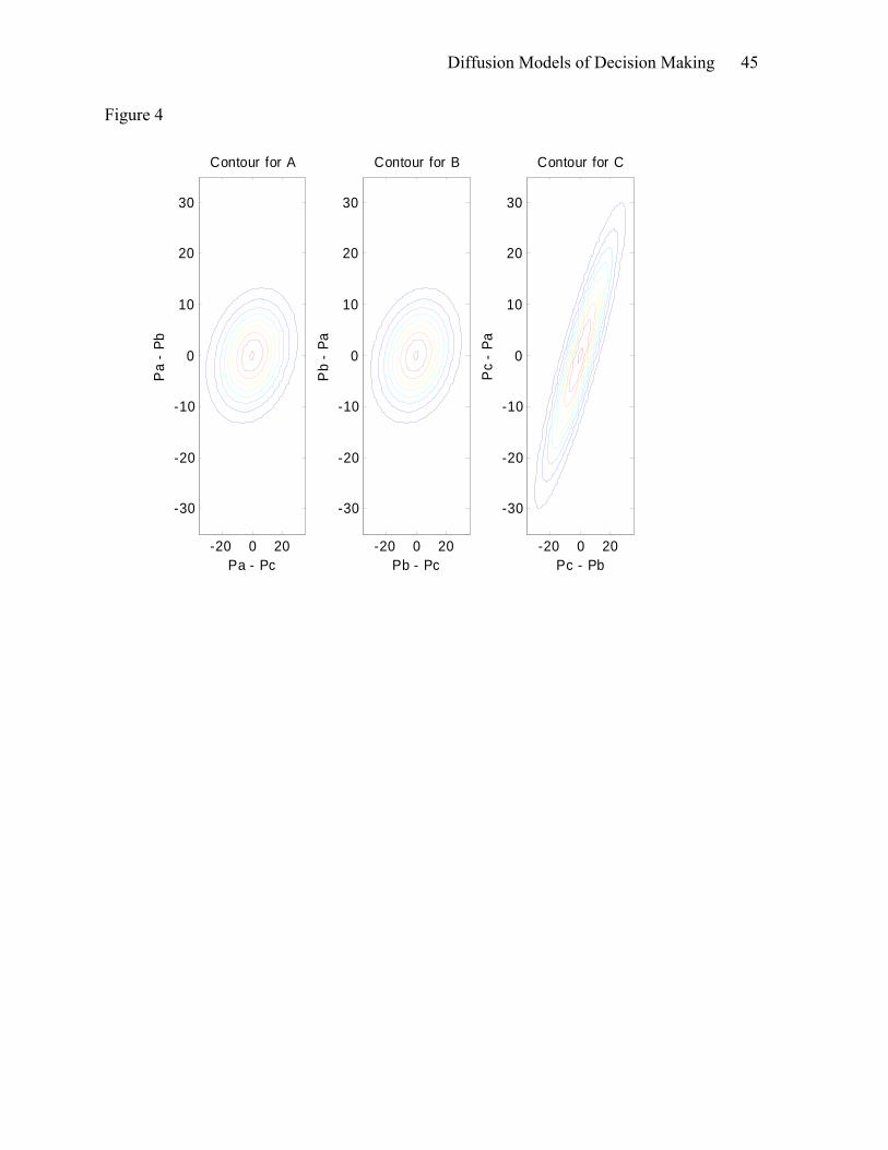
Figure 4 illustrates the effect of the covariance structure on the asymptotic

distribution of the differences in preference states (with s = .95 and b = .03). The panel on the

left shows the equal density contours for [PA(∞) – PC(∞), PA(∞) – PB(∞)]: the probability

that the preference state for A exceeds that for both B and C is the integral over the positive

right hand quadrant in this figure, which equals .29. The middle panel illustrates the equal

density contours for [PB(∞) – PC(∞), PB(∞) – PA(∞)]: the probability that the preference state

for B exceeds that for A and C is again .29. Finally, the right panel shows the equal density

contours for [PC(∞) – PB(∞), PC(∞) – PA(∞)]: the probability that the preference state for C


exceeds that for A and B equals .43. In sum, decision field theory predicts the compromise

effect as a result of the covariance structure generated by the lateral inhibitory connections

(see Roe et al., 2001, for more details).


5.3 Deliberation Time Effects on Choice

Decisions take time, and the amount of time allocated to making a decision can

change preferences. Decision field theory has been successful in accounting for a number of

findings concerning the effects of deliberation time on choice probability (see Busemeyer,

1985; Diederich, 2003; Dror, Busemeyer & Basola, 1999). Busemeyer and Townsend (1993)

discuss the ability of decision field theory to account for speed-accuracy tradeoffs that are

evident in many choice situations. That is, in general, choice probabilities are moderated with

decreases in deliberation time.

As an example, consider once again the attraction effect referred to in Figure 3:

Adding a third option Ra to the choice set increases the probability of choosing option A.

Decision field theory predicts that increasing the deliberation time increases the size of the

attraction effect. In fact, this prediction has been confirmed in several experiments

(Simonson, 1989; Dhar, Nowlis & Sherman, 2000). In other words, thinking longer actually

makes people produce stronger violations of the regularity axiom.

Equation 12 represents the asymptote of an effect that is predicted to grow during

deliberation time. The dynamic predictions of the model were computed assuming an

externally controlled stopping task, with increasing values for the stopping time T. The

predictions were generated using the coordinates of options A, B, and RA shown in Figure 3

to define the values, mjk, for each option on each dimension, wk = .50 for the mean attention


weight allocated to each dimension, sii = .95 for the self feedback, sAR = −.03 for the lateral

inhibition between the similar options A and Ra, sAB = 0 for the lateral inhibition between the

two dissimilar options A and B, and h=1. The predicted choice probabilities are plotted in

Figure 5 shown below. The choice probabilities for the binary choice lie on the .50 line; the

probability of choosing option A from the triadic choice gradually increases from .50 to

above .60; the probability of choosing option B from the triadic choice gradually decreases

from .50 to below .40; and the probability of choosing option Ra remains at zero. As can be

seen in this figure, the model correctly predicts that the attraction increases with longer

deliberation times.

Decision field theory accounts for not only moderation of preference strength, but

even reversals in preference among options as a function of deliberation time. Specifically,

Diederich (2003) found reversals in pairwise choices under time pressure, and demonstrates

the ability of decision field theory to account for her results. Decision field theory requires an

initial bias (z ≠ 0) to produce such reversals, such that the initial preference favors one

alternative whereas the valence differences tend to favor the other alternative. In this case, it

requires time for the accumulated valences to overcome the initial bias. Alternatively,

specific forms of attention switching not discussed here can be used instead to predict the

results (see Diederich, 1997, 2003, for model details). Utility theories, as static accounts of

decision making, are not able to make reasoned predictions regarding the effects of time

pressure whatsoever.



5.4 Choosing not to choose

Recently, Busemeyer, Johnson, and Jessup (in press) addressed a new phenomenon

concerning context effects reported by Dhar and Simonson (2003) that occur when an option

to ‘defer making a decision’ is included in the choice sets. Dhar and Simonson (2003) found

that adding a deferred option had opposite effects on the attraction and compromise effects –

it increased the attraction effect, and it decreased the compromise effect.

Busemeyer et al. (in press) showed that decision field theory is able to account for

these new effects using the same model specifications made for the original compromise and

attraction effects reported earlier. The only additional assumption is that the option to defer is

treated as a new choice option with values equal to the average of the values for the

presented options. This assumption produced a predicted increase in the attraction effect (by

10%) that resulted from the deferred option stealing probability away from the original

options in the binary choice set. At the same time, this assumption produced a predicted

decrease in the compromise effect (by 7%) that resulted from the deferred option decreasing

the advantage of compromise option over the other two extreme options in the triadic set.

5.5 Preference Reversals between choice and price measures

One important advantage of decision field theory is that it is not limited to choice-

based measures of preference, and it can also be extended to more complex measures such as

prices. This is important because empirically it has been found that preference orders can

reverse across choice and price measurements (Lichtenstein & Slovic, 1971, see Johnson &

Busemeyer, 2005 for a review). The basic finding is that low-variance gambles are chosen

over high-variance gambles of similar expected value, whereas the high-variance gamble

receives a higher price. Furthermore, researchers have also found discrepancies between


buying and selling prices that can be large enough to produce preference reversals. Here as

well, the buying price is greater for the low-variance gamble compared to the high-variance

gamble, but the selling prices produce the opposite rank-order (see Johnson & Busemeyer,

2005, for a review).

Johnson and Busemeyer (2005) propose that reporting a price for a gamble results

from a series of implicit comparisons between the target gamble and a set of candidate prices.

Each comparison is modeled by an implicit binary comparison process, where an implicit

choice favoring the current candidate price entails decreasing the candidate price for the next

comparison, and an implicit choice favoring the target gamble entails increasing the

candidate price for the next comparison. The comparison process continues until a price is

found that is considered equal to the target gamble—that is, a price which produces

indifference (P(t) = 0) when compared with the target gamble. Johnson and Busemeyer

(2005) show that this model accounts for a collection of response mode effects that no other

theory has been shown to successfully predict, including both types of preference reversals

mentioned above.

6. Alternate Neural Network Models for Complex Decisions

Several artificial neural network or connectionist models have been recently

developed for judgment and decision tasks (Grossberg & Gutowski, 1987; Levin & Levine,

1996; Guo & Holyoak, 2002; Holyoak & Simon, 1999; Read, Vanman, & Miller, 1997;

Usher & McClelland, 2004). The Grossberg and Gutowski (1987) model was used to explain

preference reversals between choice and prices (Section 5.5), but it has never been applied to

the phenomena discussed in Sections 5.1 to 5.4. The Levin and Levine (1996) model can

account for effects of time pressure on choice (Section 5.3), but it has not been applied


directly to any of the other phenomena reviewed here. The model by Holyoak and colleagues

has been applied to attraction effects, but it cannot account for similarity effects for binary

choices (Section 5.1), nor can it account for compromise effects for triadic choices, and it has

not been applied to preference reversals between choice and prices (Section 5.5). The Read et

al. (1997) model was designed for reasoning rather than preference problems, and so it is not

directly applicable to the phenomena reviewed here. Finally, the Usher and McClelland

(2004) model can account for similarity effects (Section 5.1), context effects (Section 5.2),

and time pressure effects (Section 5.3), but it has not been applied to the remaining

phenomena. A closer comparison with the Usher and McClelland (2004) model is presented

below.

Usher and McClelland (2004) have recently proposed the leaky competing

accumulator (LCA) model that shares many assumptions with decision field theory, but

departs from this theory on a few crucial points. This model makes different assumptions

about (a) the dynamics of response activations (what we call preference states), and (b) the

evaluations of advantages and disadvantages (what we call valences). First, they use a

nonlinear dynamic system that restricts the response activation to remain positive at all times,

whereas we use a linear dynamical system that permits positive and negative preference

states. The non-negativity restriction was imposed to be consistent with their interpretation of

response activations as neural firing rates. Second, they adopt Tversky and Kahneman’s

(1991) loss aversion hypothesis so that disadvantages have a larger impact than advantages.

Without the assumption of loss aversion, their theory is unable to account for the attraction

and compromise effects discussed in Section 5.2. Furthermore, no explanation is given


regarding the behavioral emergence of loss aversion from underlying neurophysiology.

Third, the lateral inhibition employed by LCA is not distance dependent.

It is interesting to consider why LCA does not incorporate distance dependent lateral

inhibition. An essential feature of neural networks is their use of distributed activation

patterns for representations, with similar representations sharing more activation pattern

overlap than dissimilar representations (Rumelhart & McClelland, 1986). Thus, neural

networks maintain distance dependent activation; consequently, it is only natural that they

would possess distance dependent inhibition as well. And, as has already been stated, the

striatum, a key substructure in the decision making process, is itself a network of distance

dependent laterally inhibitory neurons. So, distance dependent inhibition is more neurally

plausible than not. As to why LCA does not incorporate distant dependent inhibition, it

might be due to the notion that, coupled with the inverse S-shaped value function used to

produce loss aversion, the model would be severely hampered in its ability to account for the

compromise effect.

Usher & McClelland (2004) criticized Roe et al. (2001) because the latter model

allows for both negative as well as positive preference states, which they argue is

inconsistent with the concept of strictly positive neural activation. Busemeyer et al. (2005)

responded that the zero point of the preference scale can be interpreted as the baseline rate of

activation in neural model, with negative states representing inhibition below baseline, and

positive activation representing excitation above baseline. However, Busemeyer et al. (2005)

also formulated a nonlinear version of lateral inhibition with strictly positive states which is

also able to account for the context effects discussed in section 5.2 (see Figure 6).

Specifically, they assumed that


])([)()( btPsVtPshtdP iji

ijjjiij −⋅−+⋅=+ ∑≠

, (13)

Pj(t+h) = F[Pj(t) + dPj(t+h)], and F(x) = 0 if x < 0, F(x) = x if x ≥ 0.4 (14)

As shown in Figure 6, this version of a lateral inhibitory network still reproduces the

attraction effect while only using positive activation and positive input states.


A final criticism of decision field theory levied by Usher and McClelland (2004) is

that the model utilizes linear dynamics even though the brain is most certainly a nonlinear

system. As Busemeyer et al. (2005) argued, one reason that decision field theory has

retained linear dynamics is that mathematical solutions can be obtained for the model. And

because linear dynamics can approximate nonlinear systems, this increased mathematical

tractability comes at a minimal cost. No mathematical solutions have been derived for the

nonlinear Usher and McClelland (2004) model, and therefore one must rely on

computationally intensive Monte Carlo simulations. This issue of tractability becomes

extremely important when trying to scale up models to account for more complex measures

of preference such as prices. Computationally, it would be very difficult to model such

complex process using brute force simulations.

7. Conclusion

Models of human behavior exist on a variety of explanatory levels, tailored to

different aspects of behavior. In the field of decision making, the most popular models for

many decades have been algebraic utility models developed in economics. These models

may serve as a good first approximation to macro-level human behavior, but are severely

limited in that they only attempt to describe decision outcomes. Furthermore, their static and


deterministic nature does not allow them to account for decision dynamics and response

variability, respectively.

Recently, biologically-inspired models have been developed that focus on the

substrates of overt decision behavior. These models capture the dynamics of neural activation

that give rise to simple decisions underlying sensorimotor responses. Despite growing

interest in neuroscience among economists and decision researchers, these micro-level

models have not yet had a profound impact. Unfortunately, the majority of neuroscience by

decision researchers instead simply studies gross brain activation during traditional tasks that

is then somehow related to existing aggregate-level models.

Here, we have provided a level of analysis that we believe shows excellent potential

in bridging the gap between the customary approach of decision researchers and the

contemporary advances in neuroscience. We introduced the fundamental concepts of

modeling decision making via diffusion processes, based on decision field theory. This

approach models directly the deliberation process that results in overt choice, in line with

neural models and in contrast to algebraic utility theories. Decision field theory has also been

applied to “higher-order” cognitive tasks such as multi-attribute, multi-alternative choice and

pricing, as have utility theories (but not existing neural models of sensorimotor decisions).

Thus, diffusion models such as decision field theory seem to offer the best of both worlds

from a modeling standpoint.

Emergent properties of decision field theory allow it to explain systematic changes in

preference that have challenged the prevailing utility framework. Examples reviewed here

included applications to changes in the choice set or response method, and dependencies on


deliberation time. Decision field theory has also been shown to account for a number of other

pervasive idiosyncrasies in human decision behavior (see Busemeyer & Johnson, 2004).

Other models in the same class as decision field theory, but relying on other specific

processes, were reviewed as well. Each of these alternatives has specific advantages and

disadvantages, and they do not always make the same predictions in a given situation.

Further research is needed to discriminate between these various “bridge” models of decision

making. Regardless of exactly which model is determined to be the most successful

tomorrow, this type of modeling in general delivers superior theoretical benefits today.


References

Ashby, F. G. (2000). A stochastic version of general recognition theory. Journal of

Mathematical Psychology, 44, 310-329.

Birnbaum, M. H., Coffey, G., Mellers, B. A., & Weiss, R. (1992). Utility Measurement:

Configural weight theory and the judges point of view. Journal of Experimental

Psychology: Human Perception and Performance, 18, 331-346.

Britten, K. H., Shadlen, M. N., Newsome, W. T., & Movshon, J. A. (1993). Responses of

neurons in macaque MT to stochastic motion signals. Visual Neuroscience, 10(6),

1157-1169.

Busemeyer, J. R. (1985). Decision making under uncertainty: A comparison of simple

scalability, fixed sample, and sequential sampling models. Journal of Experimental

Psychology, 11, 538-564.

Busemeyer, J. R., & Diederich, A. (2002). Survey of decision field theory. Mathematical

Social Sciences, 43, 345-370.

Busemeyer, J. R., & Johnson, J. G. (2004). Computational models of decision making. In D.

J. Koehler & N. Harvey (Eds.), Handbook of Judgment and Decision Making (pp.

133-154). Cambridge, MA: Blackwell.

Busemeyer, J. R., Johnson, J. G., & Jessup, R. K. (in press). Preferences constructed from

dynamic micro-processing mechanisms. In S. Lichtenstein & P. Slovic (Eds.), The

Construction of Preference.

Busemeyer, J. R., & Townsend, J. T. (1992). Fundamental derivations for decision field

theory. Mathematical Social Sciences, 23, 255-282.


Busemeyer, J. R., & Townsend, J. T. (1993). Decision field theory: A dynamic-cognitive

approach to decision making in an uncertain environment. Psychological Review,

100, 432-459.

Busemeyer, J. R., Townsend, J. T., Diederich, A., & Barkan, R. (2005). Contrast effects or

loss aversion? Comment on Usher and McClelland (2004). Psychological Review,

112(1), 253-255.

Dhar, R., Nowlis, S. M., & Sherman, S. J. (2000). Trying hard or hardly trying: An analysis

of context effects in choice. Journal of Consumer Psychology, 9, 189-200.

Dhar, R., & Simonson, I. (2003). The effect of forced choice on choice. Journal of Marketing

Research, 40, 146-160.

Diederich, A. (1997). Dynamic stochastic models for decision making under time constraints.

Journal of Mathematical Psychology, 41, 260-274.

Diederich, A. (2003). MDFT account of decision making under time pressure. Psychonomic

Bulletin and Review, 10(1), 157-166.

Dror, I. E., Busemeyer, J. R., & Basola, B. (1999). Decision making under time pressure: An

independent test of sequential sampling models. Memory and Cognition, 27, 713-725.

Erev, I., & Barron, G. (2005). On Adaptation, Maximization, and Reinforcement Learning

Among Cognitive Strategies. Psychological Review, 112(4), 912-931.

Gerfen, C. R., & Wilson, C. J. (1996). The basal ganglia. In L. W. Swanson, A. Björklund &

T. Hökfelt (Eds.), Handbook of Chemical Neuroanatomy. Integrated Systems of the

CNS, Part III (Vol. 12, pp. 371-468). New York: Elsevier.

Gold, J. I. (2003). Linking reward expectation to behavior in the basal ganglia. Trends in

Neurosciences, 26(1), 12-14.


Gold, J. I., & Shadlen, M. N. (2000). Representation of a perceptual decision in developing

oculomotor commands. Nature, 404(6776), 390-394.

Gold, J. I., & Shadlen, M. N. (2001). Neural computations that underlie decisions about

sensory stimuli. Trends in Cognitive Sciences, 5(1), 10-16.

Gold, J. I., & Shadlen, M. N. (2002). Banburismus and the brain: decoding the relationship

between sensory stimuli, decisions, and reward. Neuron, 36(2), 299-308.

Grossberg, S. (1988). Neural networks and natural intelligence. Cambridge, MA: MIT Press.

Grossberg, S., & Gutowski, W. E. (1987). Neural dynamics of decision making under risk:

Affective balance and cognitive-emotional interactions. Psychological Review, 94(3),

300-318.

Guo, F. Y., & Holyoak, K. J. (2002). Understanding similarity in choice behavior: A

connectionist model. Proceedings of the Cognitive Science Society Meeting.

Heath, T. B. & Chatterjee, S. (1995). Asymmetric decoy effects on lower-quality versus

higher-quality brands: Meta analytic and experimental evidence. Journal of Consumer

Research, 22, 268-284.

Hollerman, J. R., & Schultz, W. (1998). Dopamine neurons report an error in the temporal

prediction of reward during learning. Nature Neuroscience, 1(4), 304-309.

Holyoak, K. J., & Simon, D. (1999). Bidirectional reasoning in decision making by constraint

satisfaction. Journal of Experimental Psychology: General, 128(1), 3-31.

Huber, J., & Puto, C. (1983). Market boundaries and product choice: Illustrating attraction

and substitution effects. Journal of Consumer Research, 10(1), 31-44.


Huber, J., Payne, J. W., & Puto, C. (1982). Adding asymmetrically dominated alternatives:

Violations of regularity and the similarity hypothesis. Journal of Consumer Research,

9(1), 90-98.

Johnson, J. G., & Busemeyer, J. R. (2005). A dynamic, stochastic, computational model of

preference reversal phenomena. Psychological Review, 112, 841-861.

Kahneman, D., & Tversky, A. (1979). Prospect theory: An analysis of decision under risk.

Econometrica, 47, 263-291.

Laming, D. R. (1968). Information theory of choice-reaction times. New York: Academic

Press.

Levin, S. J., & Levine, D. S. (1996). Multiattribute decision making in context: A dynamic

neural network methodology. Cognitive Science, 20, 271-299.

Lichtenstein, S., & Slovic, P. (1971). Reversals of preference between bids and choices in

gambling decisions. Journal of Experimental Psychology, 89, 46-55.

Link, S. W., & Heath, R. A. (1975). A sequential theory of psychological discrimintation.

Psychometrika, 40, 77-111.

Mazurek, M. E., Roitman, J. D., Ditterich, J., & Shadlen, M. N. (2003). A role for neural

integrators in perceptual decision making. Cerebral Cortex, 13(11), 1257-1269.

Mellers, B. A., & Biagini, K. (1994). Similarity and choice. Psychological Review, 101, 505-

518.

Middleton, F. A., & Strick, P. L. (2001). A revised neuroanatomy of frontal-subcortical

circuits. In D. G. Lichter & J. L. Cummings (Eds.), Frontal-subcortical circuits in

psychiatric and neurological disorders. (pp. 44-55). New York: Guilford Press.


Montgomery, H. (1989). From cognition to action: The search for dominance in decision

making. In H. Montgomery & O. Svenson (Eds.), Process and Structure in Human

Decision Making (pp. 23-49). New York: Wiley.

Nosofsky, R. M., & Palmeri, T. J. (1997). An exemplar-based random walk model of

speeded classification. Psychological Review, 104, 226-300.

Ratcliff, R. (1978). A theory of memory retrieval. Psychological Review, 85, 59-108.

Ratcliff, R., Cherian, A., & Segraves, M. (2003). A comparison of macaque behavior and

superior colliculus neuronal activity to predictions from models of two-choice

decisions. Journal of Neurophysiology, 90(3), 1392-1407.

Read, S. J., Vanman, E. J., & Miller, L. C. (1997). Connectionism, parallel constraint

satisfaction and gestalt principles: (Re)introducting cognitive dynamics to social

psychology. Personality and Social Psychology Review, 1, 26-53.

Rieskamp, J., Busemeyer, J. R., & Mellers, B. A. (in press). Extending the Bounds of

Rationality: A Review of Research on Preferential Choice. Journal of Economic

Literature.

Roe, R. M., Busemeyer, J. R., & Townsend, J. T. (2001). Multi-alternative decision field

theory: A dynamic connectionist model of decision-making. Psychological Review,

108, 370-392.

Rumelhart, D., & McClelland, J. L. (1986). Parallel Distributed Processing: Explorations in

the Microstructure of Cognition. Cambridge, MA: MIT Press.

Savage, L. J. (1954). Foundations of statistics. Oxford: Wiley.

Schall, J. D. (2003). Neural correlates of decision processes: neural and mental chronometry.

Current Opinion in Neurobiology, 13(2), 182-186.


Schultz, W. (1998). Predictive reward signal of dopamine neurons. Journal of

Neurophysiology, 80(1), 1-27.

Schultz, W. (2002). Getting formal with dopamine and reward. Neuron, 36(2), 241-263.

Schultz, W., Romo, R., Ljungberg, T., Mirenowicz, J., Hollerman, J. R., Dickinson, A.

(1995). Reward-related signals carried by dopamine neurons. In J. C. Houk, J. L.

Davis, & D. G. Beiser (Eds.), Models of information processing in the basal ganglia

(pp. 233-248). Cambridge, MA: MIT Press.

Shadlen, M. N., & Newsome, W. T. (2001). Neural basis of a perceptual decision in the

parietal cortex (area LIP) of the rhesus monkey. Journal of Neurophysiology, 86(4),

1916-1936.

Simonson, I. (1989). Choice based on reasons: The case of attraction and compromise

effects. Journal of Consumer Research, 16(158-174).

Smith, P. L. (1995). Psychophysically principled models of visual simple reaction time.

Psychological Review, 102(3), 567-593.

Smith, P. L., & Ratcliff, R. (2004). Psychology and neurobiology of simple decisions. Trends

in Neurosciences, 27(3), 161-168.

Solomon, R. L., & Corbit, J. D. (1974). An opponent-process theory of motivation: I.

Temporal dynamics of affect. Psychological Review, 81(2), 119-145.

Svenson, O. (1992). Differentiation and consolidation theory of human decision making: A

frame of reference for the study of pre- and post-decision processes. Acta

Psychologica, 80, 143-168.


Thagard, P., & Millgram, E. (1995). Inference to the best plan: A coherence theory of

decision. In A. Ram & D. B. Leake (Eds.), Goal-driven learning (pp. 439-454).

Cambridge, MA: MIT Press.

Tversky, A. (1969). Intransitivity of preferences. Psychological Review, 76, 31-48.

Tversky, A. (1972). Elimination by aspects: A theory of choice. Psychological Review, 79,

281-299.

Tversky, A., & Kahneman, D. (1991). Loss aversion in riskless choice: A reference

dependent model. Quarterly Journal of Economics, 106, 1039-1061.

Tversky, A., & Kahneman, D. (1992). Advances in prospect theory: Cumulative

representations of uncertainty. Journal of Risk and Uncertainty, 5, 297-323.

Tversky, A., & Simonson, I. (1993). Context dependent preferences. Management Science,

39, 1179-1189.

Usher, M., & McClelland, J. L. (2001). The time course of perceptual choice: the leaky,

competing accumulator model. Psychological Review, 108(3), 550-592.

Usher, M., & McClelland, J. L. (2004). Loss aversion and inhibition in dynamical models of

multialternative choice. Psychological Review, 111(3), 757-769.

Vickers, D., & Lee, M. D. (1998). Dynamic models of simple judgments: I. Properties of a

self-regulating accumulator module. Nonlinear Dynamics, Psychology, & Life

Sciences, 2(3), 169-194.

von Neumann, J., & Morgenstern, O. (1944). Theory of Games and Economic Behavior.

Princeton, NJ: Princeton Univ. Press.


Wedell, D. H. (1991). Distinguishing among models of contextually induced preference

reversals. Journal of Experimental Psychology: Learning, Memory, and Cognition,

17(4), 767-778.

Wickens, J. (1997). Basal ganglia: Structure and computations. Network: Computation in

Neural Systems, 8, R77-R109.

Wilson, C. J., & Groves, P. M. (1980). Fine structure and synaptic connections of the

common spiny neuron of the rat neostriatum: a study employing intracellular inject of

horseradish peroxidase. Journal of Comparative Neurology, 194(3), 599-615.


Footnotes

1. Preference is a stochastic process which should converge to a diffusion process as

h 0. The properties of preference depend upon the valence which is a random variable

because the attention weights are random. In order for preference to converge to a diffusion

process, the mean and variance must be proportional to h. And because valence is a linear

transformation of the weights, the mean and variance of the weight vector must be

proportional to h.

2. It is important to note that rarely are we faced with one option in isolation, as we

can seemingly always choose the ‘not’ option, i.e., we can choose to buy or to not buy; the

notion of ‘one option’ is rather artificial. An alternate construal might arise when the option

to choose dominates the ‘not’ option; this may be what is generally implied when it is said

that there is only one option.

3. This argument holds even if the utility of an action is computed using decision

weights for the outcomes rather than the objective state probabilities.

4. Where the usage of F corresponds to that utilized by LCA.

5. Glockner (2002) independently developed another version of the ECHO model for

decision making.


Figure Captions

Figure 1. Representation of the binary decision process in decision field theory. The

decision process begins at the start position z (often z = 0, the neutral point) and preference is

accumulated for either of the two options. The current level of accumulated preference p is

incremented by positive values of valence v and decremented by negative values. One option

is chosen when preference exceeds the upper bound θ, and the alternate option is chosen

when preference exceeds the lower bound.

Figure 2. Comparability effects. Four actions (A, B, C, & D) can be taken, and the payoffs

that are obtained depend on whether State 1 or State 2 occurs. If State 1 occurs, choice A

would yield the highest payoff and D would yield the lowest. If state 2 occurs, D would give

the highest payoff whereas C would provide the lowest. Binary choice comparisons between

the available actions elicit violations of strong stochastic transitivity and order dependence.

Unlike most utility models, decision field theory is able to explain these violations.

Figure 3. Context effects can impact decisions. Option A is high on Dimension 1 but low on

Dimension 2 whereas B is high on Dimension 2 but low on Dimension 1. Option C can be

thought of as a compromise, and options Ra and Rb can be used as reference points.

Although preference for options A and B are equivalent in binary choice comparisons,

preference for A increases when Ra is present; likewise, preference for B increases when the

choice set includes A, B, and Rb. This violation of regularity cannot be explained by

heuristic models of choice. When presented with binary comparisons involving two of A, B,

and C, preference for each option is equal. However, when all three options are

simultaneously available, option C emerges as a preferred alternative, an effect which neither

heuristic choice nor classic utility models can easily explain. Decision field theory can


explain each of these effects without even adjusting its parameters across the conditions (see

Roe et al., 2001 for other related findings).

Figure 4. Equal density contours for computing triadic choice probabilities. The leftmost

panel demonstrates the contour for the density function of option A, where positive values on

the horizontal axis indicate preference for option A over option C and positive values on the

vertical axis indicate preference for option A over B. There is a +.22 correlation in the left

panel for a choice of A, and the same is true for the middle panel (preference for B), but there

is a +.93 correlation shown in the right panel for the choice of C. This figure demonstrates

that when option C is preferred to option A, it is also very likely to be preferred to option B,

allowing it to obtain an inordinately large share of preference, whereas preference for A over

C does not indicate that it will be preferred over option B.

Figure 5. Predictions for the attraction effect as a function of deliberation time. PA2 and

PB2 indicate choice probability as a function of deliberation time for options A and B,

respectively (from Figure 3), in the binary choice condition whereas PA3 and PB3

demonstrate preference for Options A and B, respectively, during triadic choice when option

Ra is included in the choice set. Decision field theory predicts that the attraction effect

should increase with deliberation time, an effect empirically demonstrated (Simon, 1989;

Dhar et al., 2000).

Figure 6. Choice probabilities as a function of deliberation time (units on time scale are

arbitrary) for options A, B, & Rb from Figure 3, derived from a nonlinear implementation of

decision field theory that is constrained to maintain positive activation states. The nonlinear

version still reproduces the attraction effect without appealing to loss aversion.


Figure 1


Figure 2

A

BC

D

State 1

Stat

e 2


Figure 3

A

B

Ra

Rb

C

0

1

2

3

4

5

6

0 1 2 3 4 5 6

Dimension 1

Dim

ensi

on 2


Figure 4

Contour for A

Pa - Pc

Pa

- Pb

-20 0 20

-30

-20

-10

0

10

20

30

Contour for B

Pb - Pc

Pb

- Pa

-20 0 20

-30

-20

-10

0

10

20

30

Contour for C

Pc - Pb

Pc

- Pa

-20 0 20

-30

-20

-10

0

10

20

30


Figure 5

20 40 60 80 100 120 140 160 180 2000

0.1

0.2

0.3

0.4

0.5

0.6

0.7

0.8

0.9

1

Deliberation Time

Cho

ice

Pro

babi

lity

PA3PB3PA2PB2


Figure 6

building bridges between neural models

Documents