budt 725: models and applications in operations research
DESCRIPTION
BUDT 725: Models and Applications in Operations Research. by Bruce L. Golden R.H. Smith School of Business. Volume 1- Customer Relationship Management Through Data Mining. Customer Relationship Management Through Data Mining. Introduction to Customer Relationship Management (CRM) - PowerPoint PPT PresentationTRANSCRIPT

1
BUDT 725: Models and Applications
in Operations Research
by
Bruce L. Golden
R.H. Smith School of Business
Volume 1- Customer Relationship Management Through Data Mining

2
Customer Relationship ManagementThrough Data Mining
Introduction to Customer Relationship Management (CRM)
Introduction to Data Mining
Data Mining Software
Churn Modeling
Acquisition and Cross Sell Modeling

3
Relationship Marketing
Relationship Marketing is a Process
communicating with your customers
listening to their responses
Companies take actions
marketing campaigns
new products
new channels
new packaging

4
Relationship Marketing -- continued
Customers and prospects respond
most common response is no response
This results in a cycle
data is generated
opportunities to learn from the data and improve the
process emerge

5
The Move Towards Relationship Management
E-commerce companies want to customize the user experience
Supermarkets want to be infomediaries
Credit card companies want to recommend good restaurants and hotels in new cities
Phone companies want to know your friends and family
Bottom line: Companies want to be in the business of serving customers rather than merely selling products
6
CRM is Revolutionary
Grocery stores have been in the business of stocking shelves
Banks have been in the business of managing the spread between money borrowed and money lent
Insurance companies have been in the business of managing loss ratios
Telecoms have been in the business of completing telephone calls
Key point: More companies are beginning to view customers as their primary asset
7
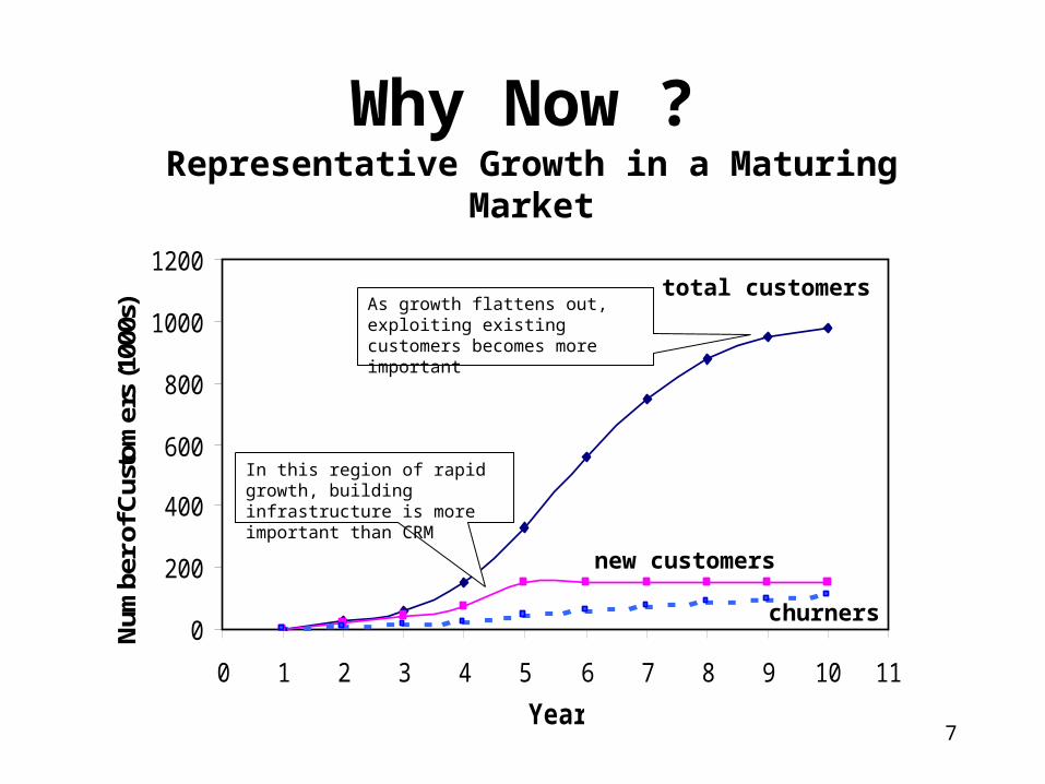
Why Now ?
0
200
400
600
800
1000
1200
0 1 2 3 4 5 6 7 8 9 10 11
Year
Num
ber
of C
usto
mer
s (1
000s
) As growth flattens out, exploiting existing customers becomes more important
In this region of rapid growth, building infrastructure is more important than CRM
total customers
new customers
churners
Representative Growth in a Maturing Market

8
The Electronic Trail
A customer places a catalog order over the telephone
At the local telephone companytime of call, number dialed, long distance company used, …
At the long distance company (for the toll-free number)
duration of call, route through switching system, …
At the catalogitems ordered, call center, promotion
response, credit card used, inventory update, shipping method requested, …
9
The Electronic Trail-- continued
At the credit card clearing housetransaction date, amount charged,
approval code, vendor number, …
At the bankbilling record, interest rate, available
credit update, …
At the package carrier zip code, time stamp at truck, time stamp at sorting center, …
Bottom line: Companies do keep track of data
10
An Illustration
A few years ago, UPS went on strike
FedEx saw its volume increase
After the strike, its volume fell
FedEx identified those customers whose FedEx volumes had increased and then decreased
These customers were using UPS again
FedEx made special offers to these customers to get all of their business
11
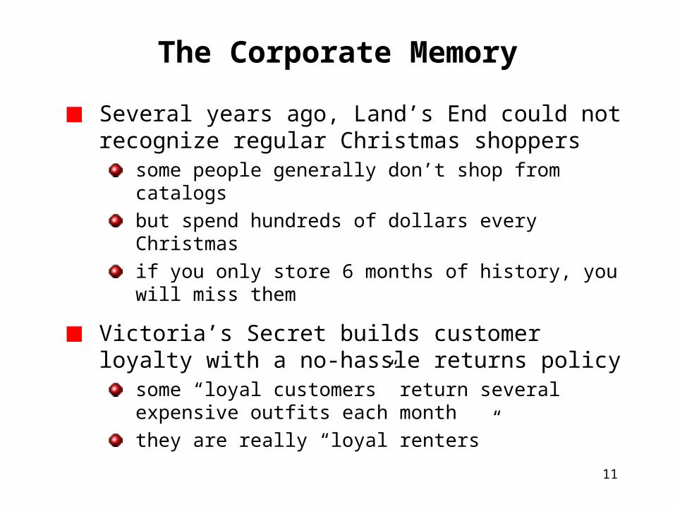
The Corporate Memory
Several years ago, Land’s End could not recognize regular Christmas shoppers
some people generally don’t shop from catalogs
but spend hundreds of dollars every Christmas
if you only store 6 months of history, you will miss them
Victoria’s Secret builds customer loyalty with a no-hassle returns policy
some “loyal customers” return several expensive outfits each month
they are really “loyal renters”
12
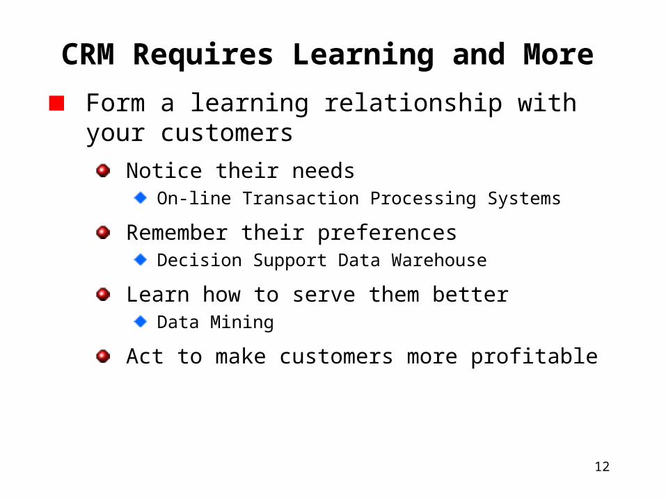
CRM Requires Learning and More
Form a learning relationship with your customers
Notice their needsOn-line Transaction Processing Systems
Remember their preferencesDecision Support Data Warehouse
Learn how to serve them betterData Mining
Act to make customers more profitable
13
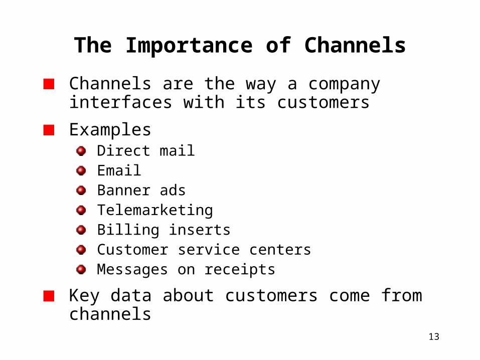
The Importance of Channels
Channels are the way a company interfaces with its customers
ExamplesDirect mailEmailBanner adsTelemarketingBilling insertsCustomer service centersMessages on receipts
Key data about customers come from channels

14
Channels -- continued
Channels are the source of data
Channels are the interface to customers
Channels enable a company to get a particular message to a particular customer
Channel management is a challenge in organizations
CRM is about serving customers through all channels

15
Where Does Data Mining Fit In?
Hindsight
Foresight
Insight
Analysis andReporting (OLAP)
StatisticalModeling
DataMining

16
Our Definition of Data Mining
Exploration and analysis of large quantities of data
By automatic or semi-automatic means
To discover meaningful patterns and rules
These patterns allow a company to
better understand its customers
improve its marketing, sales, and customer support operations
Source: Berry and Linoff (1997)
17
Data Mining for Insight
Classification
Prediction
Estimation
Automatic Cluster Detection
Affinity Grouping
Description

18
Finding Prospects
A cellular phone company wanted to introduce a new service
They wanted to know which customers were the most likely prospects
Data mining identified “sphere of influence” as a key indicator of likely prospects
Sphere of influence is the number of different telephone numbers that someone calls
19
Paying Claims
A major manufacturer of diesel engines must also service engines under warranty
Warranty claims come in from all around the world
Data mining is used to determine rules for routing claims
some are automatically approved
others require further research
Result: The manufacturer saves millions of dollars
Data mining also enables insurance companies and the Fed. Government to save millions of dollars by not paying fraudulent medical insurance claims

20
Cross Selling
Cross selling is another major application of data mining
What is the best additional or best next offer (BNO) to make to each customer?
E.g., a bank wants to be able to sell you automobile insurance when you get a car loan
The bank may decide to acquire a full-service insurance agency

21
Holding on to Good Customers
Berry and Linoff used data mining to help a major cellular company figure out who is at risk for attrition
And why are they at risk
They built predictive models to generate call lists for telemarketing
The result was a better focused, more effective retention campaign

22
Weeding out Bad Customers
Default and personal bankruptcy cost lenders millions of dollars
Figuring out who are your worst customers can be just as important as figuring out who are your best customers
many businesses lose money on most of their customers
23
They Sometimes get Their Man
The FBI handles numerous, complex cases such as the Unabomber case
Leads come in from all over the country
The FBI and other law enforcement agencies sift through thousands of reports from field agents looking for some connection
Data mining plays a key role in FBI forensics

24
Clustering is an undirected data mining technique that finds groups of similar items
Based on previous purchase patterns, customers are placed into groups
Customers in each group areassumed to have an affinityfor the same types of products
New product recommendationscan be generated automaticallybased on new purchases madeby the group
This is sometimes called collaborative filtering
Anticipating Customer Needs

25
CRM Focuses on the Customer
The enterprise has a unified view of each customer across all business units and across all channels
This is a major systems integration task
The customer has a unified view of the enterprise for all products and regardless of channel
This requires harmonizing all the channels
26
A Continuum of Customer Relationships
Large accounts have sales managers and account teams
E.g., Coca-Cola, Disney, and McDonalds
CRM tends to focus on the smaller customer --the consumer
But, small businesses are also good candidates for CRM
27
What is a Customer
A transaction?
An account?
An individual?
A household?
The customer as a transactionpurchases made with cash are anonymous
most Web surfing is anonymous
we, therefore, know little about the consumer
28
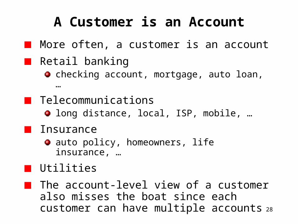
A Customer is an Account
More often, a customer is an account
Retail bankingchecking account, mortgage, auto loan, …
Telecommunicationslong distance, local, ISP, mobile, …
Insuranceauto policy, homeowners, life insurance, …
Utilities
The account-level view of a customer also misses the boat since each customer can have multiple accounts

29
Customers Play Different Roles
Parents buy back-to-school clothes for teenage children
children decide what to purchase
parents pay for the clothes
parents “own” the transaction
Parents give college-age children cellular phones or credit cards
parents may make the purchase decision
children use the product
It is not always easy to identify the customer

30
The Customer’s Lifecycle
Childhood
birth, school, graduation, …
Young Adulthoodchoose career, move away from parents, …
Family Lifemarriage, buy house, children, divorce, …
Retirementsell home, travel, hobbies, …
Much marketing effort is directed at each stage of life
31
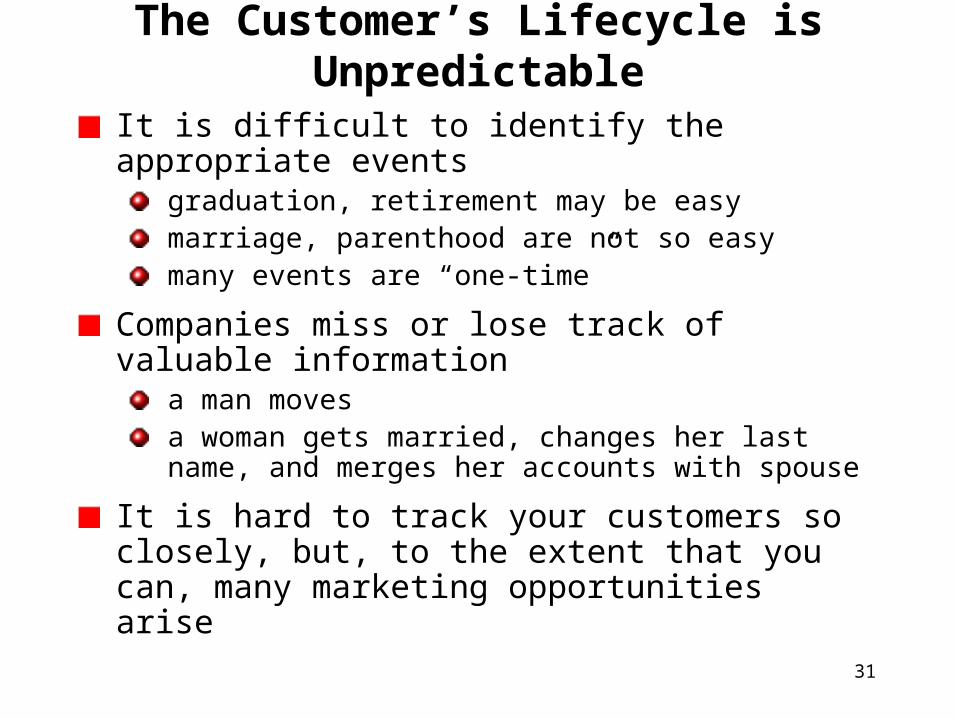
The Customer’s Lifecycle is Unpredictable
It is difficult to identify the appropriate eventsgraduation, retirement may be easymarriage, parenthood are not so easymany events are “one-time”
Companies miss or lose track of valuable information
a man movesa woman gets married, changes her last name, and merges her accounts with spouse
It is hard to track your customers so closely, but, to the extent that you can, many marketing opportunities arise
32
Customers Evolve Over Time
Customers begin as prospects
Prospects indicate interestfill out credit card applications
apply for insurance
visit your website
They become new customers
After repeated purchases or usage, they become established customers
Eventually, they become former customerseither voluntarily or involuntarily
33
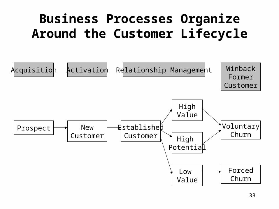
Business Processes Organize Around the Customer Lifecycle
Acquisition Activation Relationship Management WinbackFormer
Customer
Prospect EstablishedCustomer
NewCustomer
Low Value
High Potential
HighValue
VoluntaryChurn
ForcedChurn
34
Different Events OccurThroughout the Lifecycle
Prospects receive marketing messages
When they respond, they become new customers
They make initial purchases
They become established customers and are targeted by cross-sell and up-sell campaigns
Some customers are forced to leave (cancel)
Some leave (cancel) voluntarily
Others simply stop using the product (e.g., credit card)
Winback/collection campaigns
35
Different Data is AvailableThroughout the Lifecycle
The purpose of data warehousing is to keep this data around for decision-support purposes
Charles Schwab wants to handle all of their customers’ investment dollars
Schwab observed that customers started with small investments

36
Different Data is AvailableThroughout the Lifecycle -- continued
By reviewing the history of many customers, Schwab discovered that customers who transferred large amounts into their Schwab accounts did so soon after joining
After a few months, the marketing cost could not be justified
Schwab’s marketing strategy changed as a result
37
Different Models are Appropriateat Different Stages
Prospect acquisition
Prospect product propensity
Best next offer
Forced churn
Voluntary churn
Bottom line: We use data mining to predict certain events during the customer lifecycle
38
Different Approaches to Data Mining
Outsourcinglet an outside expert do the work
have him/her report the results
Off-the-shelf, turn-key software solutionspackages have generic churn models & response models
they work pretty well
Master Data Miningdevelop expertise in-house
use sophisticated software such as Clementine or Enterprise Miner

39
Privacy is a Serious Matter
Data mining and CRM raise some privacy concerns
These concerns relate to the collection of data, more than the analysis of data
The next few slides illustrate marketing mistakes that can result from the abundance and availability of data
40
Using Data Mining to Help Diabetics
Early detection of diabetes can save money by preventing more serious complicationsEarly detection of complications can prevent worsening
retinal eye exams every 6 or 12 months can prevent blindnessthese eye exams are relatively inexpensive
So one HMO took actionthey decided to encourage their members, who had diabetes to get eye examsthe IT group was asked for a list of members with diabetes

41
One Woman’s Response
Letters were sent out to HMO members
Three types of diabetes – congenital, adult-onset, gestational
One woman contacted had gestational diabetes several years earlier
She was “traumatized” by the letter, thinking the diabetes had recurred
She threatened to sue the HMO
Mistake: Disconnect between the domain expertise and data expertise
42
Gays in the Military
The “don’t ask; don’t tell” policy allows discrimination against openly gay men and lesbians in the military
Identification as gay or lesbian is sufficient grounds for discharge
This policy is enforced
Approximately 1000 involuntary discharges each year
43
The Story of Former Senior ChiefPetty Officer Timothy McVeigh
Several years ago, McVeigh used an AOL account, with an anonymous alias
Under marital status, he listed “gay”
A colleague discovered the account and called AOL to verify that the owner was McVeigh
AOL gave out the information over the phone
McVeigh was discharged (three years short of his pension)
The story doesn’t end here
44
Two Serious Privacy Violations
AOL breached its own policy by giving out confidential user information
AOL paid an undisclosed sum to settle with McVeigh and suffered bad press as well
The law requires that government agents identify themselves to get online subscription information
This was not doneMcVeigh received an honorable discharge with full retirement pension
45
Friends, Family, and Others
In the 1990s, MCI promoted the “Friends and Family” program
They asked existing customers for names of people they talked with often
If these friends and family signed up with MCI, then calls to them would be discounted
Did MCI have to ask customers about who they call regularly?
Early in 1999, BT (formerly British Telecom) took the idea one step beyond
BT invented a new marketing programdiscounts to the most frequently called numbers
46
BT Marketing Program
BT notified prospective customers of this program by sending them their most frequently called numbers
One woman received the letteruncovered her husband’s cheating
threw him out of the house
sued for divorce
The husband threatened to sue BT for violating his privacy
BT suffered negative publicity
47
No Substitute for Human Intelligence
Data mining is a tool to achieve goals
The goal is better service to customers
Only people know what to predict
Only people can make sense of rules
Only people can make sense of visualizations
Only people know what is reasonable, legal, tasteful
Human decision makers are critical to the data mining process
48
A Long, Long Time Ago
There was no marketing
There were few manufactured goods
Distribution systems were slow and uncertain
There was no credit
Most people made what they needed at home
There were no cell phones
There was no data mining
It was sufficient to build a quality product and get it to market
49
Then and Now
Before supermarkets, a typical grocery store carried 800 different items
A typical grocery store today carries tens of thousands of different items
There is intense competition for shelf space and premium shelf space
In general, there has been an explosion in the number of products in the last 50 years
Now, we need to anticipate and create demand (e.g., e-commerce)
This is what marketing is all about
50
Effective Marketing Presupposes
High quality goods and services
Effective distribution of goods and services
Adequate customer service
Marketing promises are kept
Competitiondirect (same product)
“wallet-share”
Ability to interact directly with customers
51
The ACME Corporation
Imagine a fictitious corporation that builds widgets
It can sell directly to customers via a catalog or the Web
maintain control over brand and image
It can sell directly through retail channelsget help with marketing and advertising
It can sell through resellersoutsource marketing and advertising entirely
Let’s assume ACME takes the direct marketing approach

52
Before Focusing on One-to-OneMarketing
Branding is very importantprovides a mark of quality to consumers
old concept – Bordeaux wines, Chinese porcelain, Bruges cloth
really took off in the 20th Century
Advertising is hardmedia mix problem – print, radio, TV, billboard, Web
difficult to measure effectiveness
“Half of my advertising budget is wasted; I just don’t know which half.”
53
Different Approaches to Direct Marketing
Naïve Approachget a list of potential customers
send out a large number of messages and repeat
Wave Approachsend out a large number of messages and test
Staged Approachsend a series of messages over time
Controlled Approachsend out messages over time to control response (e.g., get 10,000 responses/week)
54
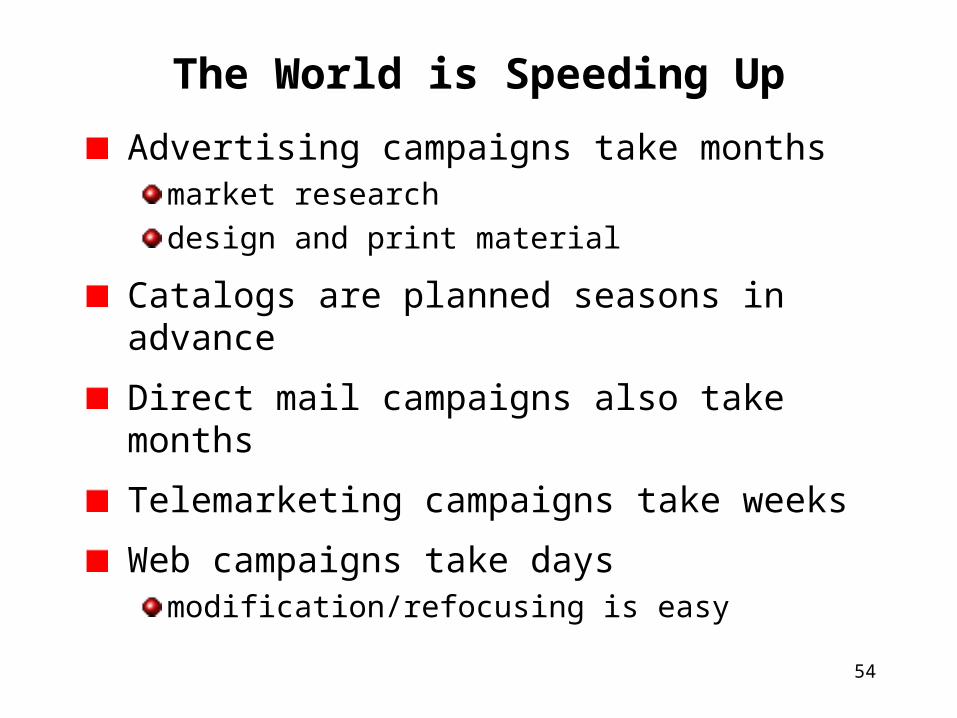
The World is Speeding Up
Advertising campaigns take monthsmarket research
design and print material
Catalogs are planned seasons in advance
Direct mail campaigns also take months
Telemarketing campaigns take weeks
Web campaigns take daysmodification/refocusing is easy

55
How Data Mining Helps inMarketing Campaigns
Improves profit by limiting campaign to most likely responders
Reduces costs by excluding individuals least likely to respond
AARP mails an invitation to those who turn 50
they excluded the bottom 10% of their list
response rate did not suffer

56
How Data Mining Helps inMarketing Campaigns--continued
Predicts response rates to help staff call centers, with inventory control, etc.
Identifies most important channel for each customer
Discovers patterns in customer data
57
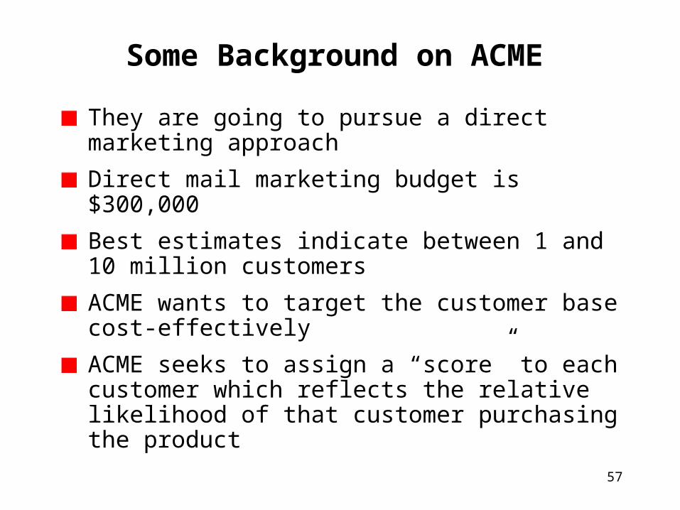
Some Background on ACME
They are going to pursue a direct marketing approach
Direct mail marketing budget is $300,000
Best estimates indicate between 1 and 10 million customers
ACME wants to target the customer base cost-effectively
ACME seeks to assign a “score” to each customer which reflects the relative likelihood of that customer purchasing the product
58
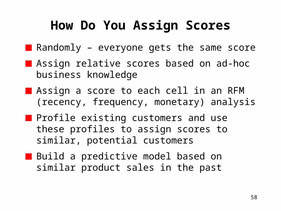
How Do You Assign Scores
Randomly – everyone gets the same score
Assign relative scores based on ad-hoc business knowledge
Assign a score to each cell in an RFM (recency, frequency, monetary) analysis
Profile existing customers and use these profiles to assign scores to similar, potential customers
Build a predictive model based on similar product sales in the past
59
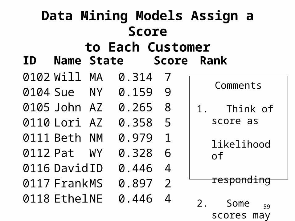
ID Name State Score Rank
0102 Will MA 0.314 70104 Sue NY 0.159 90105 John AZ 0.265 80110 Lori AZ 0.358 50111 Beth NM 0.979 10112 Pat WY 0.328 60116 David ID 0.446 40117 Frank MS 0.897 20118 Ethel NE 0.446 4
Data Mining Models Assign a Scoreto Each Customer
Comments
1. Think of score as likelihood of responding
2. Some scores may be the same
60
Approach 1: Budget Optimization
ACME has a budget of $300,000 for a direct mail campaign
Assumptionseach item being mailed costs $1this cost assumes a minimum order of 20,000
ACME can afford to contact 300,000 customers
ACME contacts the highest scoring 300,000 customers
Let’s assume ACME is selecting from the top three deciles
61
The Concept of Lift
If we look at a random 10% of the potential customers, we expect to get 10% of likely responders
Can we select 10% of the potential customers and get more than 10% of likely responders?
If so, we realize “lift”
This is a key goal in data mining
62
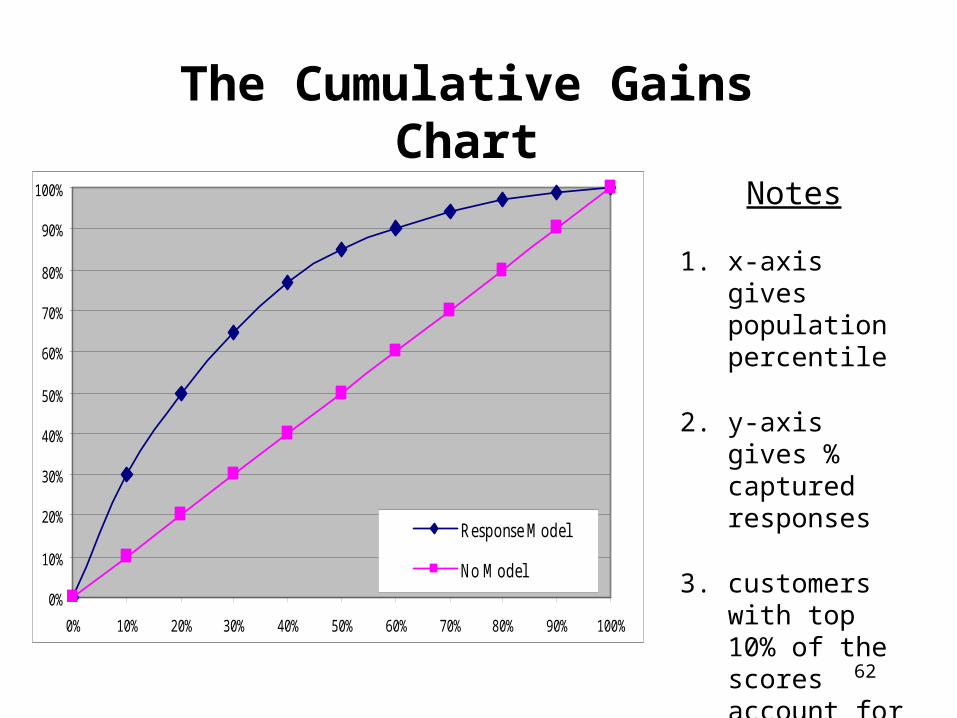
Notes
1. x-axis gives population percentile
2. y-axis gives % captured responses
3. customers with top 10% of the scores account for 30% of responders
The Cumulative Gains Chart
0%
10%
20%
30%
40%
50%
60%
70%
80%
90%
100%
0% 10% 20% 30% 40% 50% 60% 70% 80% 90% 100%
Response Model
No Model
63
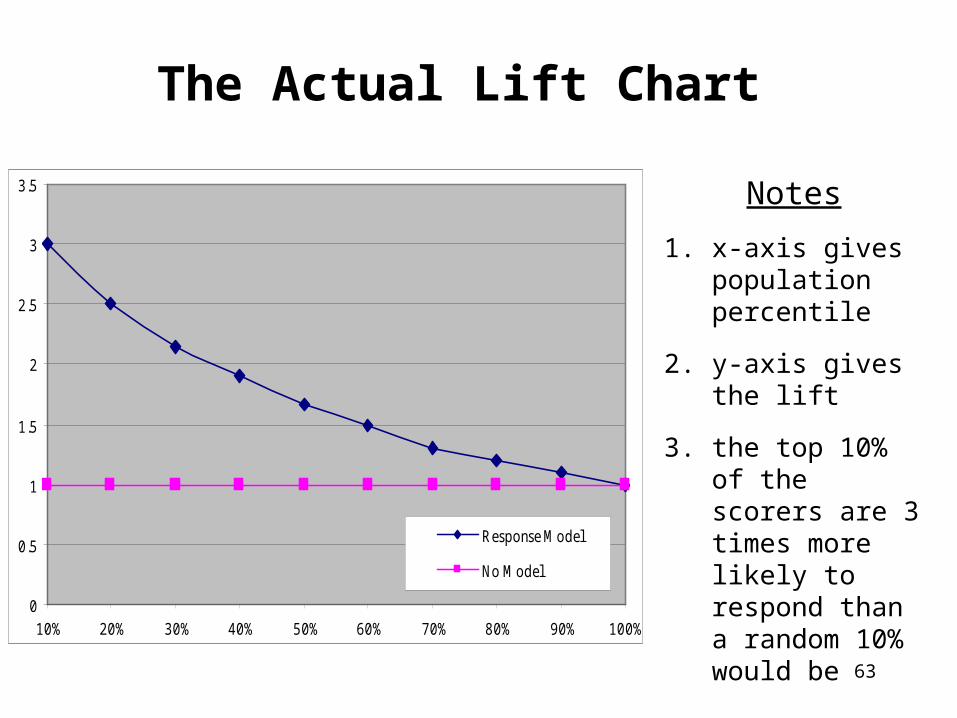
Notes
1. x-axis gives population percentile
2. y-axis gives the lift
3. the top 10% of the scorers are 3 times more likely to respond than a random 10% would be
The Actual Lift Chart
0
0.5
1
1.5
2
2.5
3
3.5
10% 20% 30% 40% 50% 60% 70% 80% 90% 100%
Response Model
No Model

64
How Well Does ACME Do?
ACME selects customers from the top three deciles
From cumulative gains chart, a response rate of 65% (vs. 30%) results
From lift chart, we see a lift of 65/30 = 2.17
The two charts convey the same information, but in different ways
65
Can ACME Do Better?
Test marketing campaignsend a mailing to a subset of the customers, say 30,000
take note of the 1 to 2% of those who respond
build predictive models to predict response
use the results from these models
The key is to learn from the test marketing campaign
66
Optimizing the Budget
Decide on the budget
Based on cost figures, determine the size of the mailing
Develop a model to score all customers with respect to their relative likelihood to respond to the offer
Choose the appropriate number of top scoring customers

67
Approach 2: Optimizing the Campaign
Lift allows us to contact more of the potential responders
It is a very useful measure
But, how much better off are we financially?
We seek a profit-and-loss statement for the campaign
To do this, we need more information than before
68
Is the Campaign Profitable?
Suppose the followingthe typical customer will purchase about $100 worth of merchandise from the next catalog
of the $100, $55 covers the cost of inventory, warehousing, shipping, and so on
the cost of sending mail to each customer is $1
Then, the net revenue per customer in the campaign is $100 - $55 - $1 = $44
69
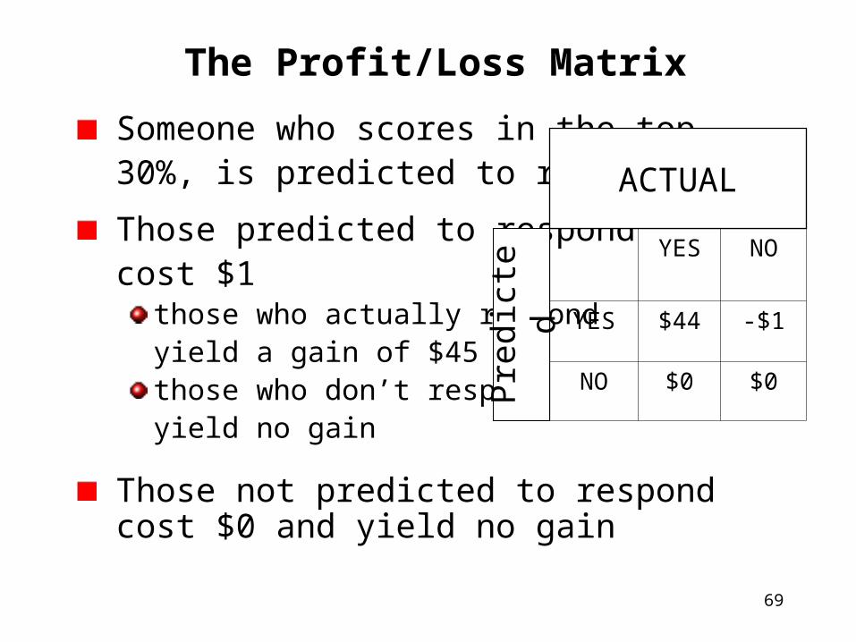
Someone who scores in the top 30%, is predicted to respond
Those predicted to respond cost $1
those who actually respondyield a gain of $45those who don’t respondyield no gain
Those not predicted to respond cost $0 and yield no gain
The Profit/Loss Matrix
YES NO
YES $44 -$1
NO $0 $0
ACTUAL
Pre
dict
ed
70
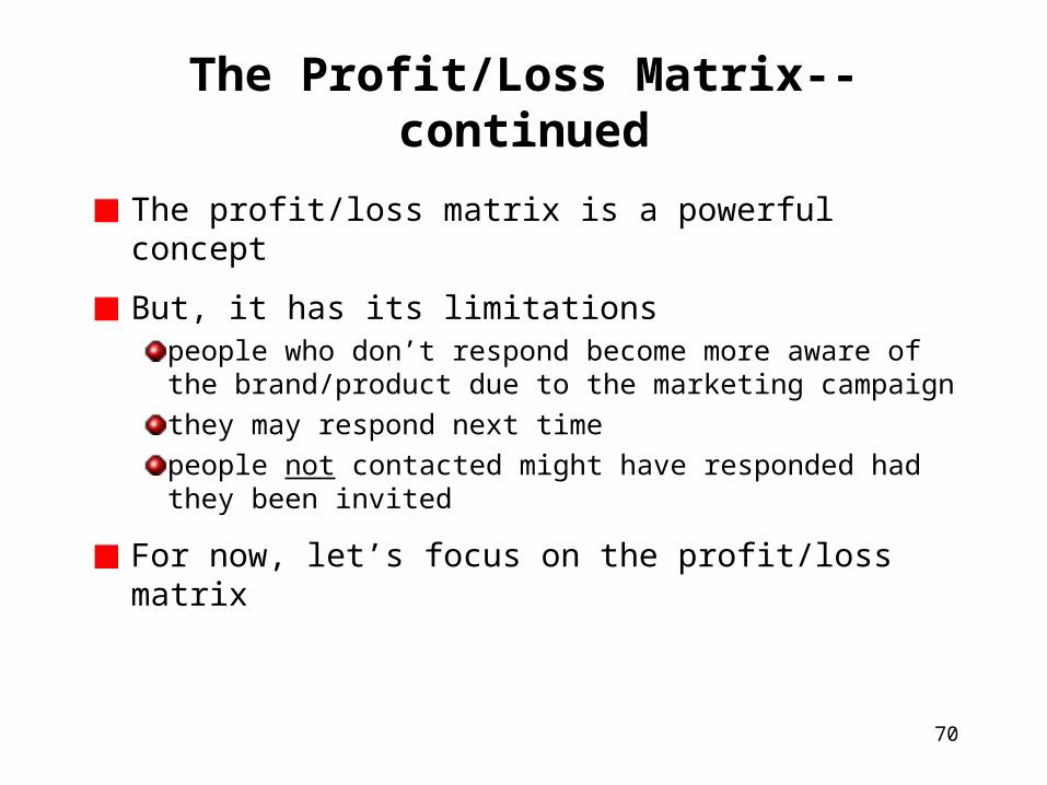
The Profit/Loss Matrix--continued
The profit/loss matrix is a powerful concept
But, it has its limitationspeople who don’t respond become more aware of the brand/product due to the marketing campaign
they may respond next time
people not contacted might have responded had they been invited
For now, let’s focus on the profit/loss matrix
71
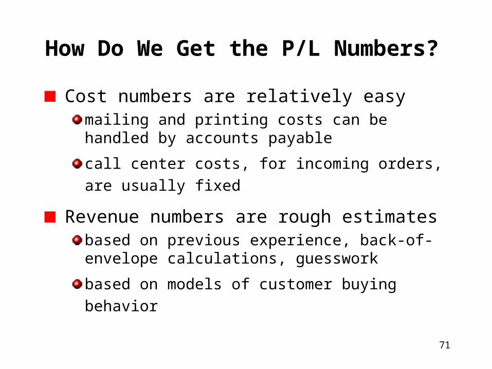
How Do We Get the P/L Numbers?
Cost numbers are relatively easymailing and printing costs can be handled by accounts payable
call center costs, for incoming orders, are usually fixed
Revenue numbers are rough estimatesbased on previous experience, back-of-envelope calculations, guesswork
based on models of customer buying behavior
72
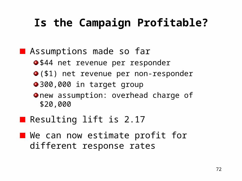
Is the Campaign Profitable?
Assumptions made so far$44 net revenue per responder
($1) net revenue per non-responder
300,000 in target group
new assumption: overhead charge of $20,000
Resulting lift is 2.17
We can now estimate profit for different response rates
73
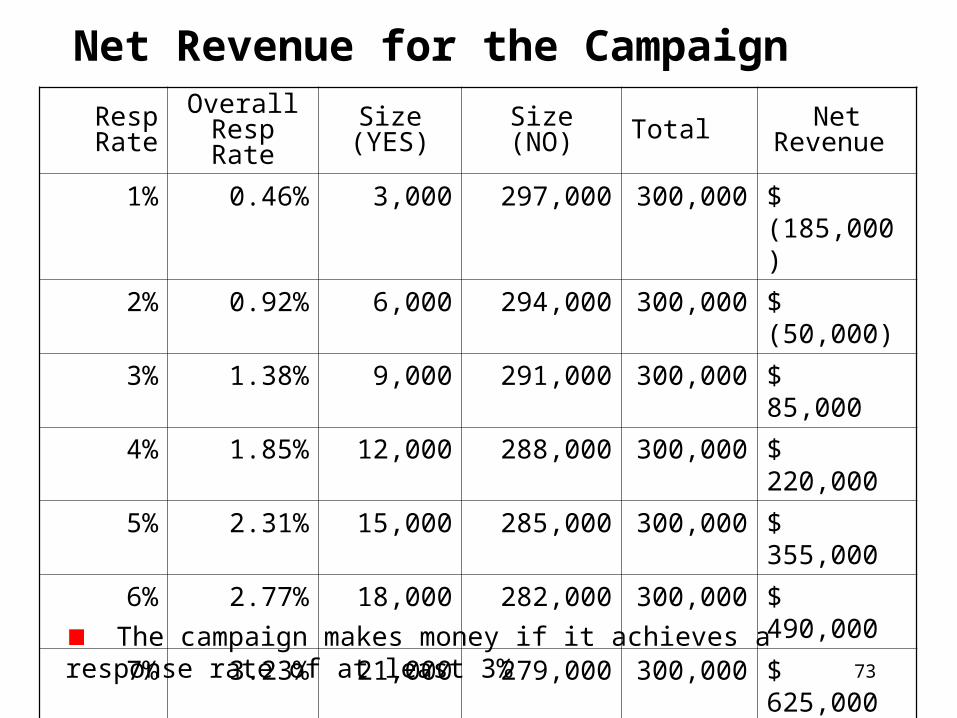
Net Revenue for the Campaign
The campaign makes money if it achieves a response rate of at least 3%
Resp Rate OverallResp Rate
Size(YES)
Size(NO) Total Net Revenue
1% 0.46% 3,000 297,000 300,000 $ (185,000)
2% 0.92% 6,000 294,000 300,000 $ (50,000)
3% 1.38% 9,000 291,000 300,000 $ 85,000
4% 1.85% 12,000 288,000 300,000 $ 220,000
5% 2.31% 15,000 285,000 300,000 $ 355,000
6% 2.77% 18,000 282,000 300,000 $ 490,000
7% 3.23% 21,000 279,000 300,000 $ 625,000
8% 3.69% 24,000 276,000 300,000 $ 760,000
9% 4.15% 27,000 273,000 300,000 $ 895,000
10% 4.62% 30,000 270,000 300,000 $ 1,030,000
74
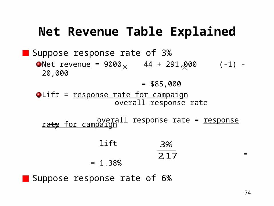
Suppose response rate of 3%Net revenue = 9000 44 + 291,000 (-1) - 20,000
= $85,000
Lift = response rate for campaign overall response rate
overall response rate = response rate for campaign lift
= = 1.38%
Suppose response rate of 6%
Net Revenue Table Explained
172
3
.
%

75
Two Ways to Estimate Response Rates
Use a randomly selected hold-out set (the test set)this data is not used to build the model
the model’s performance on this set estimates the performance on unseen data
Use a hold-out set on oversampled datamost data mining involves binary outcomes
often, we try to predict a rare event (e.g., fraud)
with oversampling, we overrepresent the rare outcomes and underrepresent the common outcomes

76
Oversampling Builds Better Models for Rare Events
Suppose 99% of records involve no fraud
A model that always predicts no fraud will be hard to beat
But, such a model is not useful
Stratified sampling with two outcomes is called oversampling
77
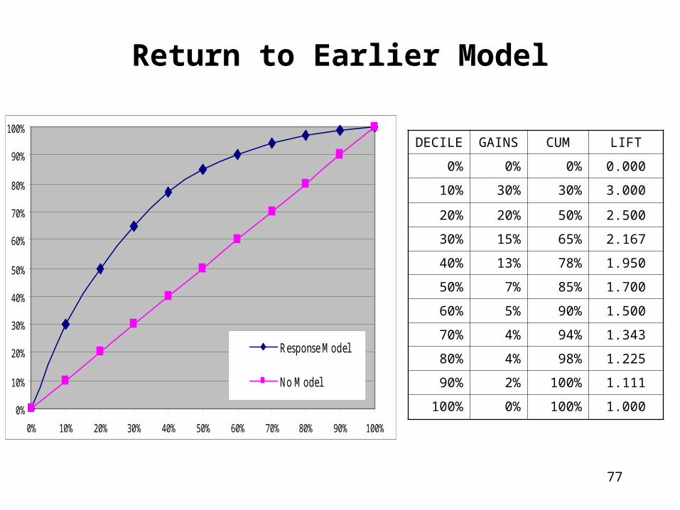
Return to Earlier Model
0%
10%
20%
30%
40%
50%
60%
70%
80%
90%
100%
0% 10% 20% 30% 40% 50% 60% 70% 80% 90% 100%
Response Model
No Model
DECILE GAINS CUM LIFT
0% 0% 0% 0.000
10% 30% 30% 3.000
20% 20% 50% 2.500
30% 15% 65% 2.167
40% 13% 78% 1.950
50% 7% 85% 1.700
60% 5% 90% 1.500
70% 4% 94% 1.343
80% 4% 98% 1.225
90% 2% 100% 1.111
100% 0% 100% 1.000
78
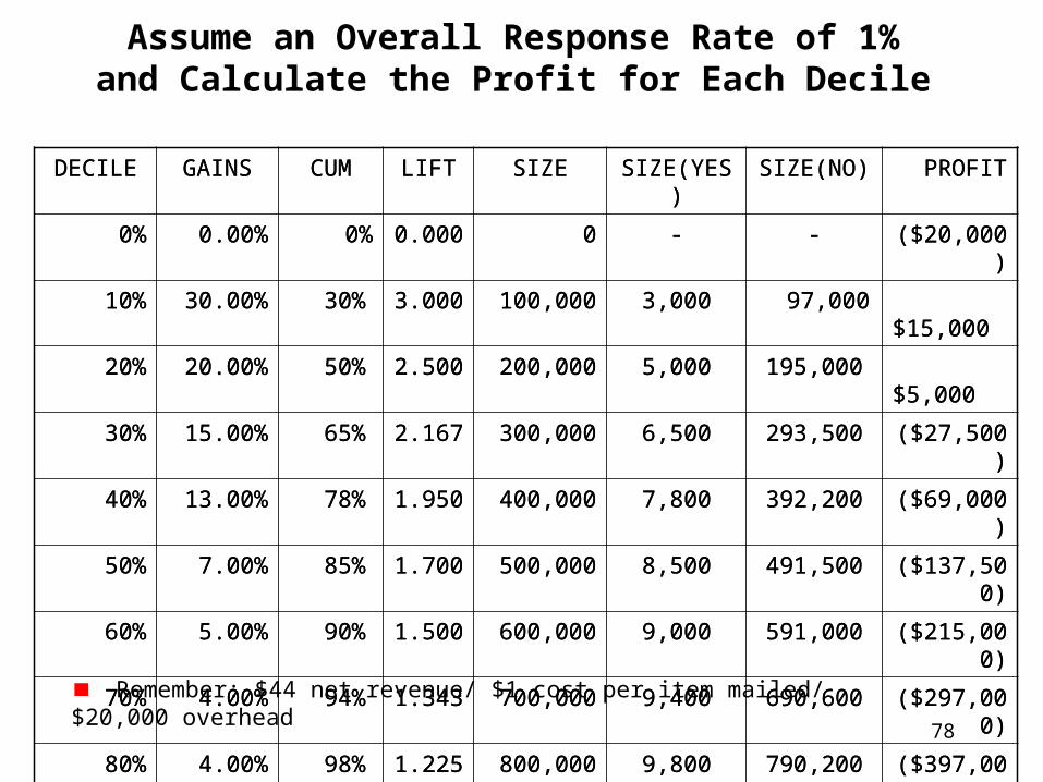
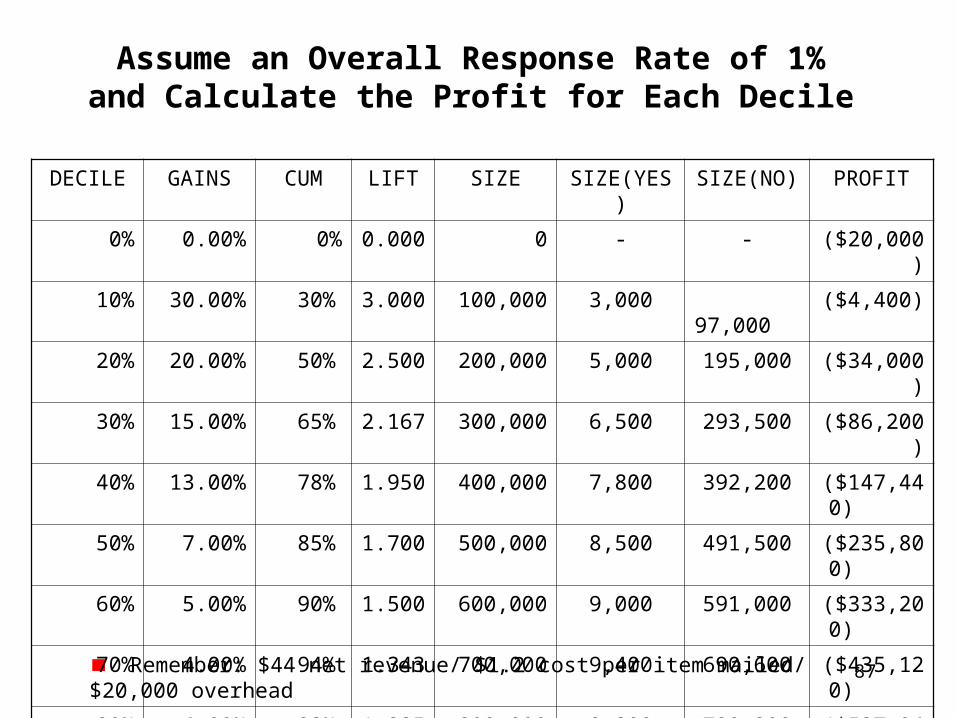
Assume an Overall Response Rate of 1%and Calculate the Profit for Each Decile
DECILE GAINS CUM LIFT SIZE SIZE(YES) SIZE(NO) PROFIT
0% 0.00% 0% 0.000 0 - - ($20,000)
10% 30.00% 30% 3.000 100,000 3,000 97,000 $15,000
20% 20.00% 50% 2.500 200,000 5,000 195,000 $5,000
30% 15.00% 65% 2.167 300,000 6,500 293,500 ($27,500)
40% 13.00% 78% 1.950 400,000 7,800 392,200 ($69,000)
50% 7.00% 85% 1.700 500,000 8,500 491,500 ($137,500)
60% 5.00% 90% 1.500 600,000 9,000 591,000 ($215,000)
70% 4.00% 94% 1.343 700,000 9,400 690,600 ($297,000)
80% 4.00% 98% 1.225 800,000 9,800 790,200 ($397,000)
90% 2.00% 100% 1.111 900,000 10,000 890,000 ($470,000)
100% 0.00% 100% 1.000 1,000,000 10,000 990,000 ($570,000)
Remember: $44 net revenue/ $1 cost per item mailed/ $20,000 overhead
DECILE GAINS CUM LIFT SIZE SIZE(YES) SIZE(NO) PROFIT
0% 0.00% 0% 0.000 0 - - ($20,000)
10% 30.00% 30% 3.000 100,000 3,000 97,000 $15,000
20% 20.00% 50% 2.500 200,000 5,000 195,000 $5,000
30% 15.00% 65% 2.167 300,000 6,500 293,500 ($27,500)
40% 13.00% 78% 1.950 400,000 7,800 392,200 ($69,000)
50% 7.00% 85% 1.700 500,000 8,500 491,500 ($137,500)
60% 5.00% 90% 1.500 600,000 9,000 591,000 ($215,000)
70% 4.00% 94% 1.343 700,000 9,400 690,600 ($297,000)
80% 4.00% 98% 1.225 800,000 9,800 790,200 ($397,000)
90% 2.00% 100% 1.111 900,000 10,000 890,000 ($470,000)
100% 0.00% 100% 1.000 1,000,000 10,000 990,000 ($570,000)

79
Key equationssize (yes) = lift
profit = 44 size (yes) - size (no) - 20,000
Example: top three deciles (30% row)
size (yes) = 2.167 = 6500
profit = 286,000 - 293,500 - 20,000
= -27,500
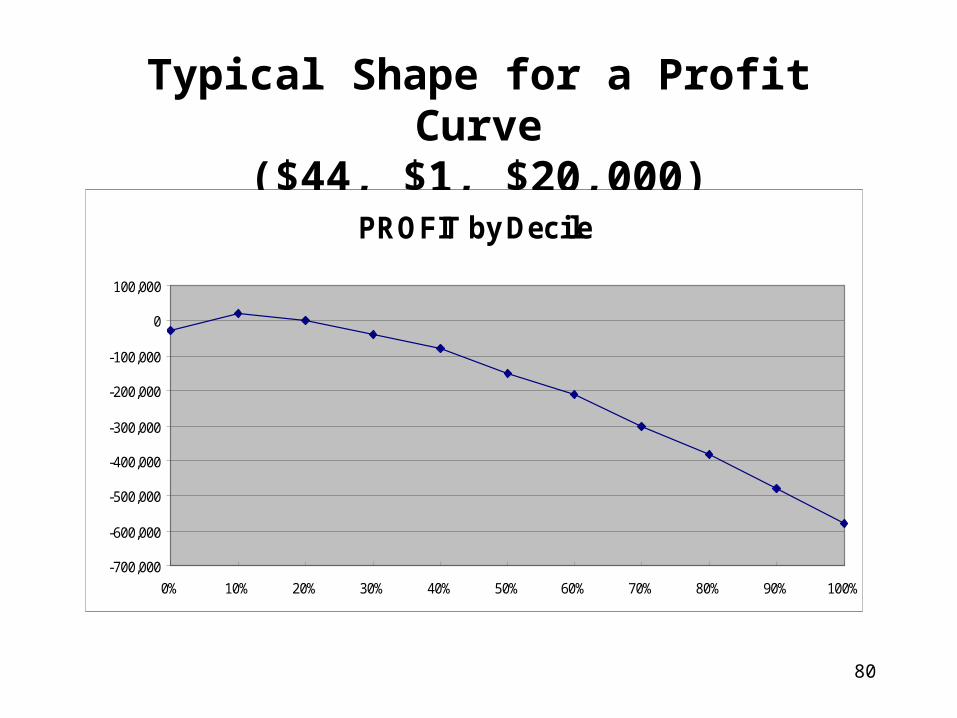
Notice that top 10% yields the maximum profit
Mailing to the top three deciles would cost us money
Review of Profit Calculation
100
000300,
100
size
80
Typical Shape for a Profit Curve($44, $1, $20,000)
PROFIT by Decile
-700,000
-600,000
-500,000
-400,000
-300,000
-200,000
-100,000
0
100,000
0% 10% 20% 30% 40% 50% 60% 70% 80% 90% 100%
81
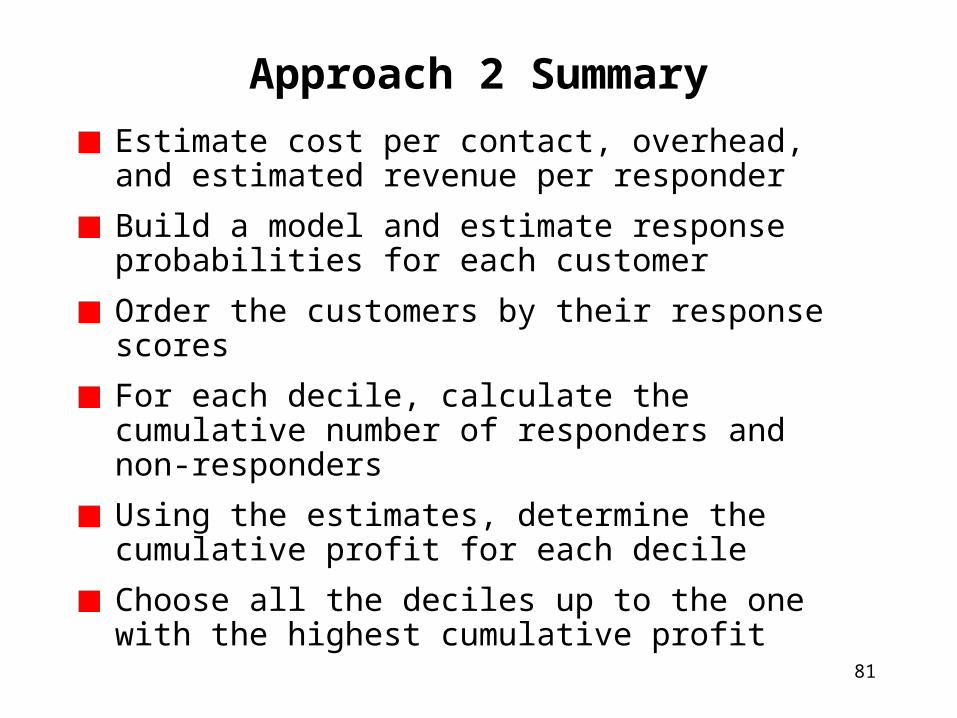
Approach 2 Summary
Estimate cost per contact, overhead, and estimated revenue per responder
Build a model and estimate response probabilities for each customer
Order the customers by their response scores
For each decile, calculate the cumulative number of responders and non-responders
Using the estimates, determine the cumulative profit for each decile
Choose all the deciles up to the one with the highest cumulative profit
82
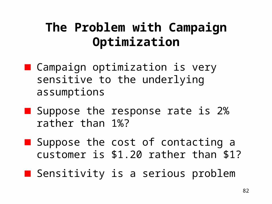
The Problem with Campaign Optimization
Campaign optimization is very sensitive to the underlying assumptions
Suppose the response rate is 2% rather than 1%?
Suppose the cost of contacting a customer is $1.20 rather than $1?
Sensitivity is a serious problem
83
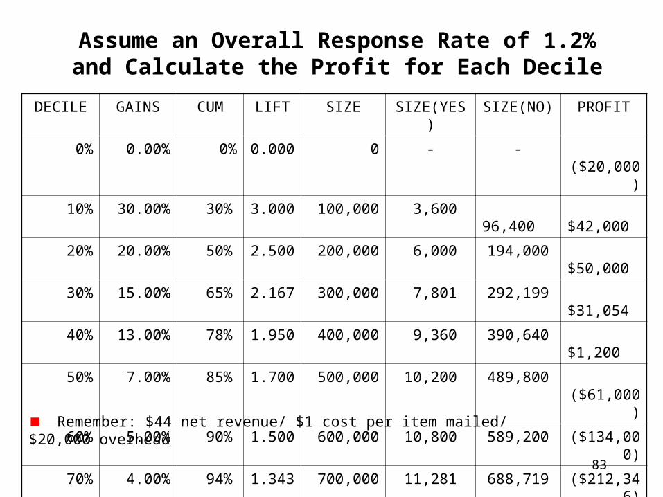
Assume an Overall Response Rate of 1.2%and Calculate the Profit for Each Decile
DECILE GAINS CUM LIFT SIZE SIZE(YES) SIZE(NO) PROFIT
0% 0.00% 0% 0.000 0 - - ($20,000)
10% 30.00% 30% 3.000 100,000 3,600 96,400 $42,000
20% 20.00% 50% 2.500 200,000 6,000 194,000 $50,000
30% 15.00% 65% 2.167 300,000 7,801 292,199 $31,054
40% 13.00% 78% 1.950 400,000 9,360 390,640 $1,200
50% 7.00% 85% 1.700 500,000 10,200 489,800 ($61,000)
60% 5.00% 90% 1.500 600,000 10,800 589,200 ($134,000)
70% 4.00% 94% 1.343 700,000 11,281 688,719 ($212,346)
80% 4.00% 98% 1.225 800,000 11,760 788,240 ($290,800)
90% 2.00% 100% 1.111 900,000 11,999 888,001 ($380,054)
100% 0.00% 100% 1.000 1,000,000 12,000 988,000 ($480,000)
Remember: $44 net revenue/ $1 cost per item mailed/ $20,000 overhead
84
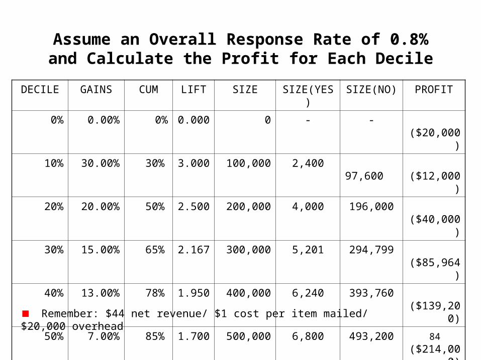
DECILE GAINS CUM LIFT SIZE SIZE(YES) SIZE(NO) PROFIT
0% 0.00% 0% 0.000 0 - - ($20,000)
10% 30.00% 30% 3.000 100,000 2,400 97,600 ($12,000)
20% 20.00% 50% 2.500 200,000 4,000 196,000 ($40,000)
30% 15.00% 65% 2.167 300,000 5,201 294,799 ($85,964)
40% 13.00% 78% 1.950 400,000 6,240 393,760 ($139,200)
50% 7.00% 85% 1.700 500,000 6,800 493,200 ($214,000)
60% 5.00% 90% 1.500 600,000 7,200 592,800 ($296,000)
70% 4.00% 94% 1.343 700,000 7,521 692,479 ($381,564)
80% 4.00% 98% 1.225 800,000 7,840 792,160 ($467,200)
90% 2.00% 100% 1.111 900,000 7,999 892,001 ($560,036)
100% 0.00% 100% 1.000 1,000,000 8,000 992,000 ($660,000)
Remember: $44 net revenue/ $1 cost per item mailed/ $20,000 overhead
Assume an Overall Response Rate of 0.8%and Calculate the Profit for Each Decile

85
DECILE GAINS CUM LIFT SIZE SIZE(YES) SIZE(NO) PROFIT
0% 0.00% 0% 0.000 0 - - ($20,000)
10% 30.00% 30% 3.000 100,000 6,000 94,000 $150,000
20% 20.00% 50% 2.500 200,000 10,000 190,000 $230,000
30% 15.00% 65% 2.167 300,000 13,002 286,998 $265,090
40% 13.00% 78% 1.950 400,000 15,600 384,400 $282,000
50% 7.00% 85% 1.700 500,000 17,000 483,000 $245,000
60% 5.00% 90% 1.500 600,000 18,000 582,000 $190,000
70% 4.00% 94% 1.343 700,000 18,802 681,198 $126,090
80% 4.00% 98% 1.225 800,000 19,600 780,400 $62,000
90% 2.00% 100% 1.111 900,000 19,998 880,002 ($20,090)
100% 0.00% 100% 1.000 1,000,000 20,000 980,000 ($120,000)
Remember: $44 net revenue/ $1 cost per item mailed/ $20,000 overhead
Assume an Overall Response Rate of 2%and Calculate the Profit for Each Decile
86
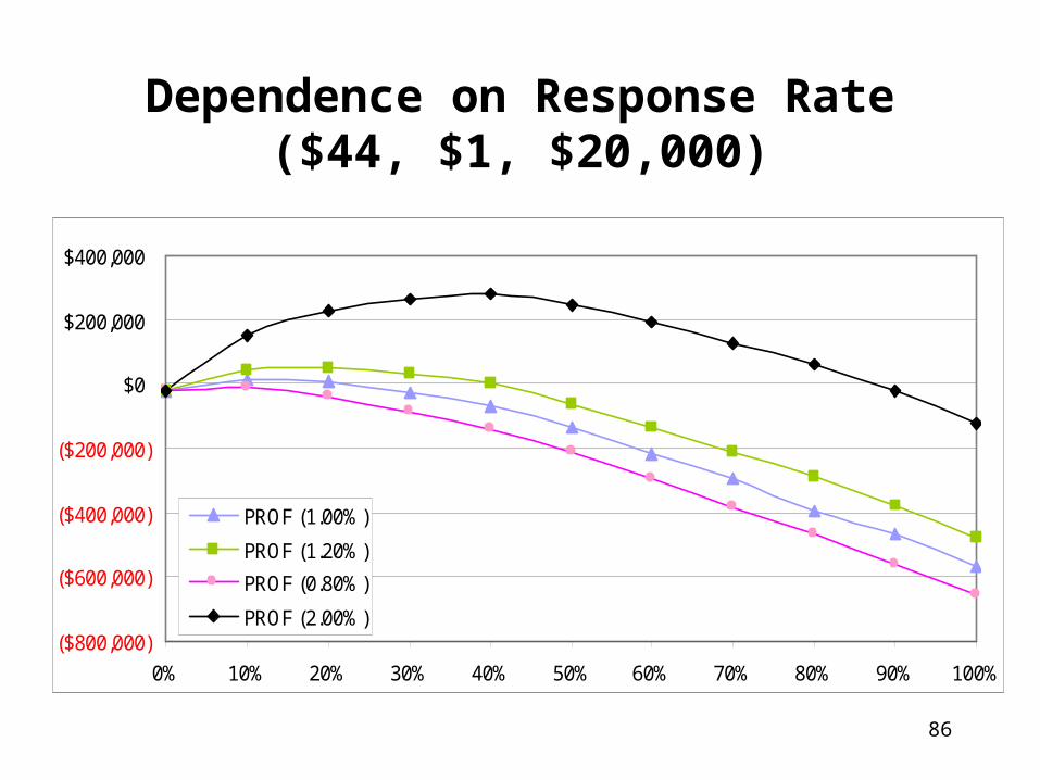
Dependence on Response Rate($44, $1, $20,000)
($800,000)
($600,000)
($400,000)
($200,000)
$0
$200,000
$400,000
0% 10% 20% 30% 40% 50% 60% 70% 80% 90% 100%
PROF (1.00%)
PROF (1.20%)
PROF (0.80%)
PROF (2.00%)
87
Assume an Overall Response Rate of 1%and Calculate the Profit for Each Decile
Remember: $44 net revenue/ $1.2 cost per item mailed/ $20,000 overhead
DECILE GAINS CUM LIFT SIZE SIZE(YES) SIZE(NO) PROFIT
0% 0.00% 0% 0.000 0 - - ($20,000)
10% 30.00% 30% 3.000 100,000 3,000 97,000 ($4,400)
20% 20.00% 50% 2.500 200,000 5,000 195,000 ($34,000)
30% 15.00% 65% 2.167 300,000 6,500 293,500 ($86,200)
40% 13.00% 78% 1.950 400,000 7,800 392,200 ($147,440)
50% 7.00% 85% 1.700 500,000 8,500 491,500 ($235,800)
60% 5.00% 90% 1.500 600,000 9,000 591,000 ($333,200)
70% 4.00% 94% 1.343 700,000 9,400 690,600 ($435,120)
80% 4.00% 98% 1.225 800,000 9,800 790,200 ($537,040)
90% 2.00% 100% 1.111 900,000 10,000 890,000 ($648,000)
100% 0.00% 100% 1.000 1,000,000 10,000 990,000 ($768,000)
88
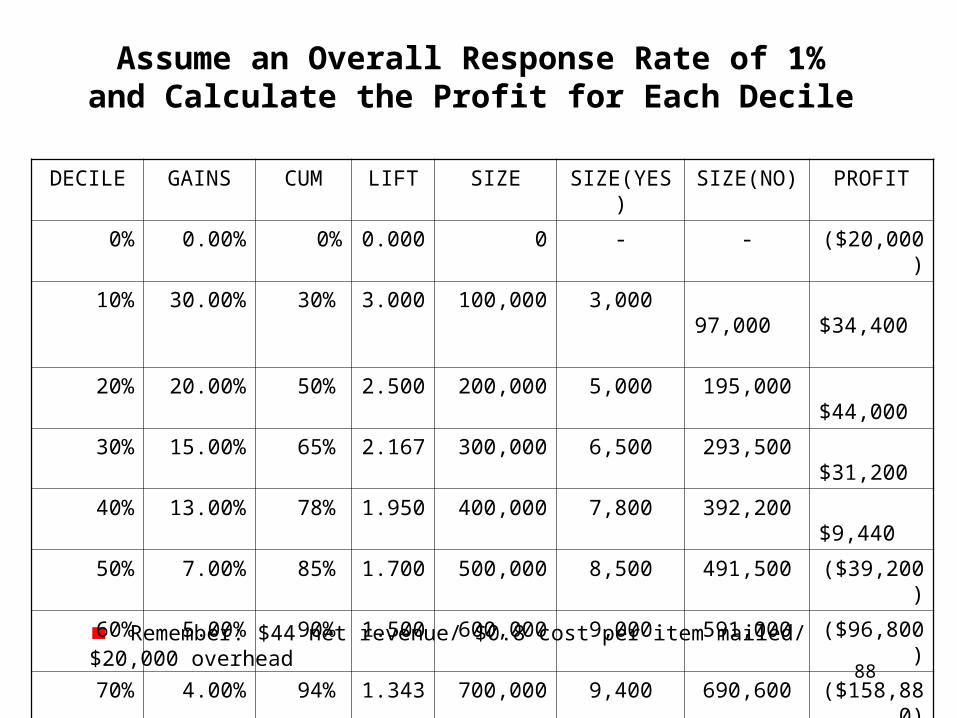
Assume an Overall Response Rate of 1%and Calculate the Profit for Each Decile
Remember: $44 net revenue/ $0.8 cost per item mailed/ $20,000 overhead
DECILE GAINS CUM LIFT SIZE SIZE(YES) SIZE(NO) PROFIT
0% 0.00% 0% 0.000 0 - - ($20,000)
10% 30.00% 30% 3.000 100,000 3,000 97,000 $34,400
20% 20.00% 50% 2.500 200,000 5,000 195,000 $44,000
30% 15.00% 65% 2.167 300,000 6,500 293,500 $31,200
40% 13.00% 78% 1.950 400,000 7,800 392,200 $9,440
50% 7.00% 85% 1.700 500,000 8,500 491,500 ($39,200)
60% 5.00% 90% 1.500 600,000 9,000 591,000 ($96,800)
70% 4.00% 94% 1.343 700,000 9,400 690,600 ($158,880)
80% 4.00% 98% 1.225 800,000 9,800 790,200 ($220,000)
90% 2.00% 100% 1.111 900,000 10,000 890,000 ($292,000)
100% 0.00% 100% 1.000 1,000,000 10,000 990,000 ($372,000)
89
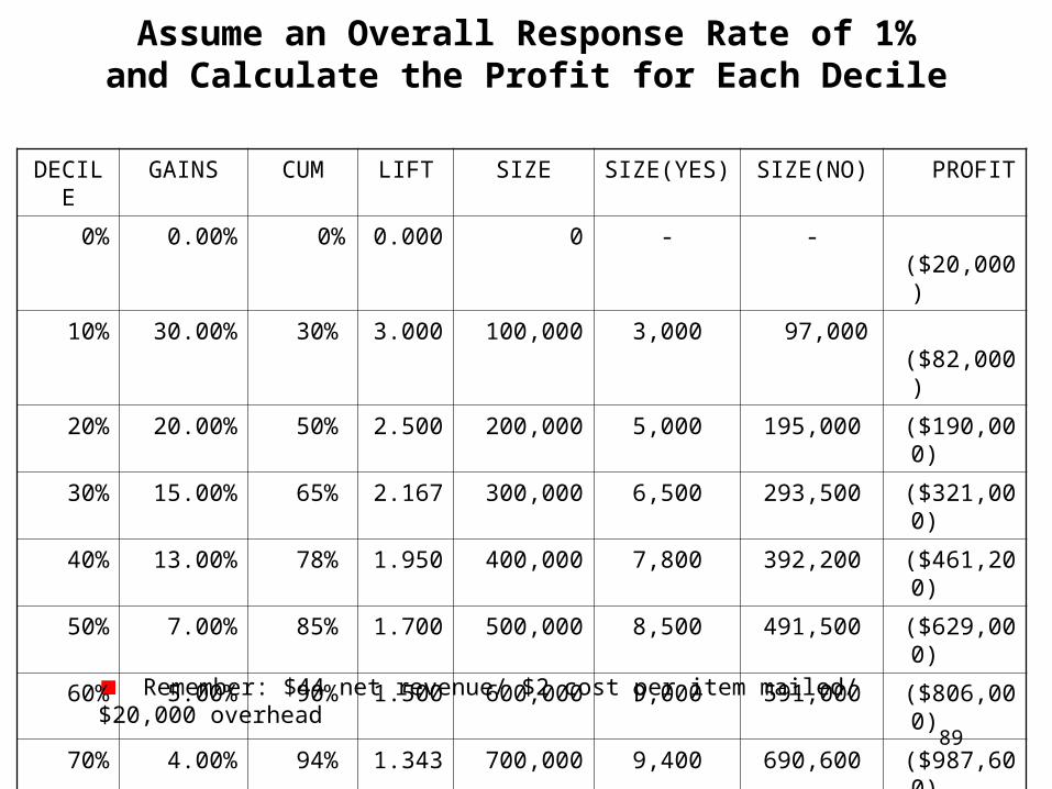
Assume an Overall Response Rate of 1%and Calculate the Profit for Each Decile
Remember: $44 net revenue/ $2 cost per item mailed/ $20,000 overhead
DECILE
GAINS CUM LIFT SIZE SIZE(YES) SIZE(NO) PROFIT
0% 0.00% 0% 0.000 0 - - ($20,000)
10% 30.00% 30% 3.000 100,000 3,000 97,000 ($82,000)
20% 20.00% 50% 2.500 200,000 5,000 195,000 ($190,000)
30% 15.00% 65% 2.167 300,000 6,500 293,500 ($321,000)
40% 13.00% 78% 1.950 400,000 7,800 392,200 ($461,200)
50% 7.00% 85% 1.700 500,000 8,500 491,500 ($629,000)
60% 5.00% 90% 1.500 600,000 9,000 591,000 ($806,000)
70% 4.00% 94% 1.343 700,000 9,400 690,600 ($987,600)
80% 4.00% 98% 1.225 800,000 9,800 790,200 ($1,169,200)
90% 2.00% 100% 1.111 900,000 10,000 890,000 ($1,360,000)
100% 0.00% 100% 1.000 1,000,000 10,000 990,000 ($1,560,000)

90
($1,800,000)
($1,600,000)
($1,400,000)
($1,200,000)
($1,000,000)
($800,000)
($600,000)
($400,000)
($200,000)
$0
$200,000
0% 10% 20% 30% 40% 50% 60% 70% 80% 90% 100%
PROF ($1)
PROF ($1.20)
PROF ($0.80)
PROF ($2.00)
Dependence on Costs
91
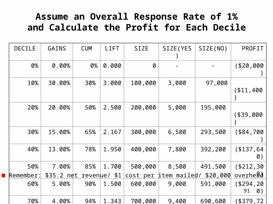
Assume an Overall Response Rate of 1%and Calculate the Profit for Each Decile
Remember: $35.2 net revenue/ $1 cost per item mailed/ $20,000 overhead
DECILE GAINS CUM LIFT SIZE SIZE(YES) SIZE(NO) PROFIT
0% 0.00% 0% 0.000 0 - - ($20,000)
10% 30.00% 30% 3.000 100,000 3,000 97,000 ($11,400)
20% 20.00% 50% 2.500 200,000 5,000 195,000 ($39,000)
30% 15.00% 65% 2.167 300,000 6,500 293,500 ($84,700)
40% 13.00% 78% 1.950 400,000 7,800 392,200 ($137,640)
50% 7.00% 85% 1.700 500,000 8,500 491,500 ($212,300)
60% 5.00% 90% 1.500 600,000 9,000 591,000 ($294,200)
70% 4.00% 94% 1.343 700,000 9,400 690,600 ($379,720)
80% 4.00% 98% 1.225 800,000 9,800 790,200 ($465,240)
90% 2.00% 100% 1.111 900,000 10,000 890,000 ($558,000)
100% 0.00% 100% 1.000 1,000,000 10,000 990,000 ($658,000)
92
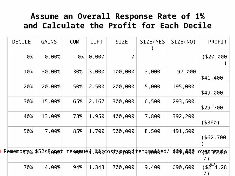
Assume an Overall Response Rate of 1%and Calculate the Profit for Each Decile
Remember: $52.8 net revenue/ $1 cost per item mailed/ $20,000 overhead
DECILE GAINS CUM LIFT SIZE SIZE(YES) SIZE(NO) PROFIT
0% 0.00% 0% 0.000 0 - - ($20,000)
10% 30.00% 30% 3.000 100,000 3,000 97,000 $41,400
20% 20.00% 50% 2.500 200,000 5,000 195,000 $49,000
30% 15.00% 65% 2.167 300,000 6,500 293,500 $29,700
40% 13.00% 78% 1.950 400,000 7,800 392,200 ($360)
50% 7.00% 85% 1.700 500,000 8,500 491,500 ($62,700)
60% 5.00% 90% 1.500 600,000 9,000 591,000 ($135,800)
70% 4.00% 94% 1.343 700,000 9,400 690,600 ($214,280)
80% 4.00% 98% 1.225 800,000 9,800 790,200 ($292,760)
90% 2.00% 100% 1.111 900,000 10,000 890,000 ($382,000)
100% 0.00% 100% 1.000 1,000,000 10,000 990,000 ($482,000)

93
Assume an Overall Response Rate of 1%and Calculate the Profit for Each Decile
Remember: $88 net revenue/ $1 cost per item mailed/ $20,000 overhead
DECILE GAINS CUM LIFT SIZE SIZE(YES) SIZE(NO) PROFIT
0% 0.00% 0% 0.000 0 - - ($20,000)
10% 30.00% 30% 3.000 100,000 3,000 97,000 $147,000
20% 20.00% 50% 2.500 200,000 5,000 195,000 $225,000
30% 15.00% 65% 2.167 300,000 6,500 293,500 $258,500
40% 13.00% 78% 1.950 400,000 7,800 392,200 $274,200
50% 7.00% 85% 1.700 500,000 8,500 491,500 $236,500
60% 5.00% 90% 1.500 600,000 9,000 591,000 $181,000
70% 4.00% 94% 1.343 700,000 9,400 690,600 $116,600
80% 4.00% 98% 1.225 800,000 9,800 790,200 $52,200
90% 2.00% 100% 1.111 900,000 10,000 890,000 ($30,000)
100% 0.00% 100% 1.000 1,000,000 10,000 990,000 ($130,000)
94
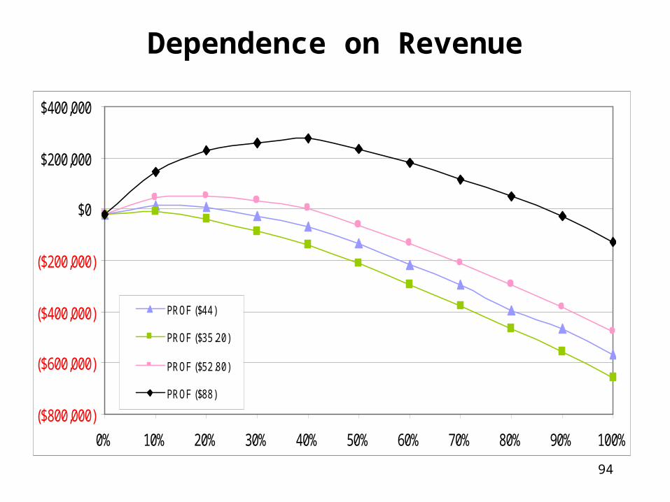
($800,000)
($600,000)
($400,000)
($200,000)
$0
$200,000
$400,000
0% 10% 20% 30% 40% 50% 60% 70% 80% 90% 100%
PROF ($44)
PROF ($35.20)
PROF ($52.80)
PROF ($88)
Dependence on Revenue

95
Campaign Optimization Drawbacks
Profitability depends on response rates, cost estimates, and revenue potential
Each one impacts profitability
The numbers we use are just estimates
If we are off by a little here and a little there, our profit estimates could be off by a lot
In addition, the same group of customers is chosen for multiple campaigns

96
Approach 3: Customer Optimization
Campaign optimization makes a lot of sense
But, campaign profitability is difficult to estimate
Is there a better way?
Do what is best for each customer
Focus on customers, rather than campaigns
97
Real-World Campaigns
Companies usually have several products that they want to sell
telecom: local, long distance, mobile, ISP, etc.banking: CDs, mortgages, credit cards, etc.insurance: home, car, personal liability, etc.retail: different product lines
There are also upsell and customer retention programs
These campaigns compete for customers

98
Each Campaign May Have a Separate Model
These models produce scores
The score tells us how likely a given customer is to respond to that specific campaign
0, if the customer already has the product0, if the product and customer are incompatible1, if the customer has asked about the product
Each campaign is relevant for a subset of all the customers
Imagine three marketing campaigns, each with a separate data mining model
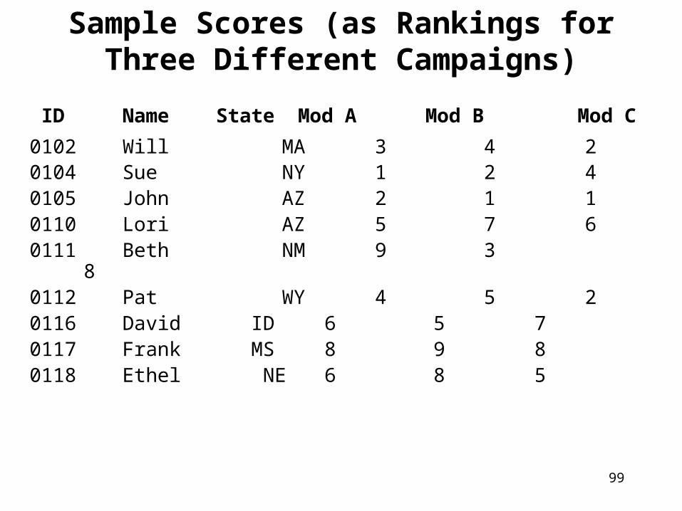
99
Sample Scores (as Rankings for Three Different Campaigns)
ID Name State Mod A Mod B Mod C
0102 Will MA 3 4 20104 Sue NY 1 2 40105 John AZ 2 1 10110 Lori AZ 5 7 60111 Beth NM 9 3 80112 Pat WY 4 5 20116 David ID 6 5 70117 Frank MS 8 9 80118 Ethel NE 6 8 5
100
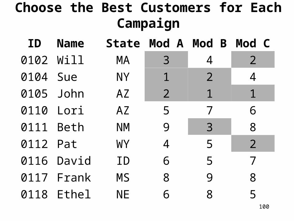
Choose the Best Customers for Each Campaign
ID Name State Mod A Mod B Mod C
0102 Will MA 3 4 2
0104 Sue NY 1 2 4
0105 John AZ 2 1 1
0110 Lori AZ 5 7 6
0111 Beth NM 9 3 8
0112 Pat WY 4 5 2
0116 David ID 6 5 7
0117 Frank MS 8 9 8
0118 Ethel NE 6 8 5

101
A Common Situation
“Good” customers are typically targeted by many campaigns
Many other customers are not chosen for any campaigns
Good customers who become inundated with contacts become less likely to respond at all
Let the campaigns compete for customers
102
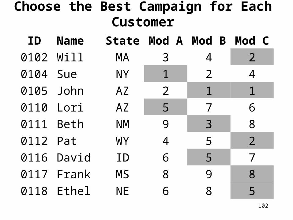
Choose the Best Campaign for Each Customer
ID Name State Mod A Mod B Mod C
0102 Will MA 3 4 2
0104 Sue NY 1 2 4
0105 John AZ 2 1 1
0110 Lori AZ 5 7 6
0111 Beth NM 9 3 8
0112 Pat WY 4 5 2
0116 David ID 6 5 7
0117 Frank MS 8 9 8
0118 Ethel NE 6 8 5
103
Focus on the Customer
Determine the propensity of each customer to respond to each campaign
Estimate the net revenue for each customer from each campaign
Incorporate profitability into the customer-optimization strategy
Not all campaigns will apply to all customers

104
First, Determine Response Rate for Each Campaign
ID Name State Mod A Mod B Mod C
102 Will MA 2.0% 0.9% 0.0%
104 Sue NY 8.0% 1.4% 3.7%
105 John AZ 3.8% 2.3% 11.0%
110 Lori AZ 0.9% 7.0% 1.3%
111 Beth NM 0.1% 1.2% 0.8%
112 Pat WY 2.0% 0.8% 4.6%
116 David ID 0.8% 0.8% 1.1%
117 Frank MS 0.2% 0.2% 0.8%
118 Ethel NE 0.8% 0.2% 0.0%
Customers who are not candidates are given a rate of zero

105
Second, Add in Product Profitability
ID Name State Mod A Mod B Mod C Prof A Prof B Prof C
102 Will MA 2.0% 0.9% 0.0% $56 $72 $20
104 Sue NY 8.0% 1.4% 3.7% $56 $72 $20
105 John AZ 3.8% 2.3% 11.0% $56 $72 $20
110 Lori AZ 0.9% 7.0% 1.3% $56 $72 $20
111 Beth NM 0.1% 1.2% 0.8% $56 $72 $20
112 Pat WY 2.0% 0.8% 4.6% $56 $72 $20
116 David ID 0.8% 0.8% 1.1% $56 $72 $20
117 Frank MS 0.2% 0.2% 0.8% $56 $72 $20
118 Ethel NE 0.8% 0.2% 0.0% $56 $72 $20
As a more sophisticated alternative, profit could be estimated for each customer/product combination

106
Finally, Determine the Campaign with the Highest Value
ID Name State EP (A) EP (B) EP (C) Campaign
102 Will MA $1.12 $0.65 $0.00 A
104 Sue NY $4.48 $1.01 $0.74 A
105 John AZ $2.13 $1.66 $2.20 C
110 Lori AZ $0.50 $5.04 $0.26 B
111 Beth NM $0.06 $0.86 $0.16 B
112 Pat WY $1.12 $0.58 $0.92 A
116 David ID $0.45 $ 0.58 $0.22 B
117 Frank MS $0.11 $0.14 $0.16 C
118 Ethel NE $0.45 $0.14 $0.00 A
EP (k) = the expected profit of product k For each customer, choose the highest expected profit campaign

107
Conflict Resolution with Multiple Campaigns
Managing many campaigns at the same time is complex
for technical and political reasons
Who owns the customer?
Handling constraintseach campaign is appropriate for a subset of customers
each campaign has a minimum and maximum number of contacts
each campaign seeks a target response rate
new campaigns emerge over time
108
Marketing Campaigns and CRM
The simplest approach is to optimize the budget using the rankings that models produce
Campaign optimization determines the most profitable subset of customers for a given campaign, but it is sensitive to assumptions
Customer optimization is more sophisticated
It chooses the most profitable campaign for each customer
109
The Data Mining Process
What role does data mining play within an organization?
How does one do data mining correctly?
The SEMMA Processselect and sample
explore
modify
model
assess
110
Identify the Right Business Problem
Involve the business users
Have them provide business expertise, not technical expertise
Define the problem clearly“predict the likelihood of churn in the next month for our 10% most valuable customers”
Define the solution clearlyis this a one-time job, an on-going monthly batch job, or a real-time response (call centers and web)?
What would the ideal result look like?how would it be used?
111
Transforming the Data into Actionable Information
Select and sample by extracting a portion of a large data set-- big enough to contain significant information, but small enough to manipulate quickly
Explore by searching for unanticipated trends and anomalies in order to gain understanding

112
Modify by creating, selecting, and transforming the variables to focus the model selection process
Model by allowing the software to search automatically for a combination of variables that reliably predicts a desired outcome
Assess by evaluating the usefulness and reliability of the findings from the data mining process
Transforming the Data into Actionable Information-- continued
113
Act on Results
Marketing/retention campaign lists or scores
Personalized messages
Customized user experience
Customer prioritization
Increased understanding of customers, products, messages

114
Measure the Results
Confusion matrix
Cumulative gains chart
Lift chart
Estimated profit
115
Data Mining Uses Data from the Past to Effect Future Action
“Those who do not remember the past are condemned to repeat it.” – George Santayana
Analyze available data (from the past)
Discover patterns, facts, and associations
Apply this knowledge to future actions
116
Examples
Prediction uses data from the past to make predictions about future events (“likelihoods” and “probabilities”)
Profiling characterizes past events and assumes that the future is similar to the past (“similarities”)
Description and visualization find patterns in past data and assume that the future is similar to the past

117
We Want a Stable Model
A stable model works (nearly) as well on unseen data as on the data used to build it
Stability is more important than raw performance for most applications
we want a car that performs well on real roads, not just on test tracks
Stability is a constant challenge
118
Is the Past Relevant?
Does past data contain the important business drivers?
e.g., demographic data
Is the business environment from the past relevant to the future?
in the ecommerce era, what we know about the past may not be relevant to tomorrow
users of the web have changed since late 1990s
Are the data mining models created from past data relevant to the future?
have critical assumptions changed?
119
Data Mining is about Creating Models
A model takes a number of inputs, which often come from databases, and it produces one or more outputs
Sometimes, the purpose is to build the best model
The best model yields the most accurate output
Such a model may be viewed as a black box
Sometimes, the purpose is to better understand what is happening
This model is more like a gray box
120
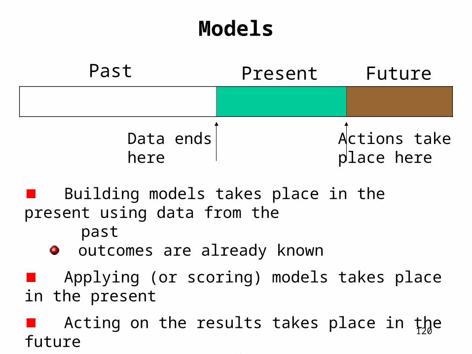
Models
Past Present Future
Data endshere
Actions takeplace here
Building models takes place in the present using data from the past
outcomes are already known
Applying (or scoring) models takes place in the present
Acting on the results takes place in the future outcomes are not known

121
Often, the Purpose is to Assign a Scoreto Each Customer
ID Name State Score
1 0102 Will MA 0.314
2 0104 Sue NY 0.159
3 0105 John AZ 0.265
4 0110 Lori AZ 0.358
5 0111 Beth NM 0.979
6 0112 Pat WY 0.328
7 0116 David ID 0.446
8 0117 Frank MS 0.897
9 0118 Ethel NE 0.446
Comments
1. Scores are assigned to rows using models
2. Some scores may be the same
3. The scores may represent the probability of some outcome

122
Common Examples of What a Score Could Mean
Likelihood to respond to an offer
Which product to offer next
Estimate of customer lifetime
Likelihood of voluntary churn
Likelihood of forced churn
Which segment a customer belongs to
Similarity to some customer profile
Which channel is the best way to reach the customer
123
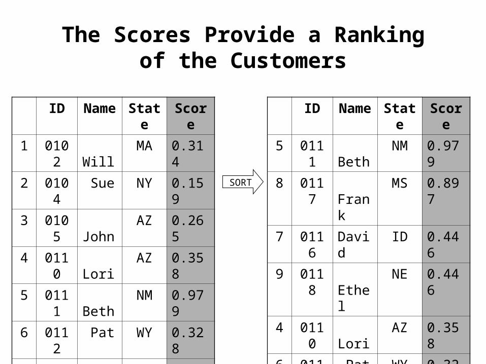
The Scores Provide a Rankingof the Customers
ID Name State Score
1 0102 Will MA 0.314
2 0104 Sue NY 0.159
3 0105 John AZ 0.265
4 0110 Lori AZ 0.358
5 0111 Beth NM 0.979
6 0112 Pat WY 0.328
7 0116 David ID 0.446
8 0117 Frank MS 0.897
9 0118 Ethel NE 0.446
ID Name State Score
5 0111 Beth NM 0.979
8 0117 Frank
MS 0.897
7 0116 David ID 0.446
9 0118 Ethel NE 0.446
4 0110 Lori AZ 0.358
6 0112 Pat WY 0.328
1 0102 Will MA 0.314
3 0105 John AZ 0.265
2 0104 Sue NY 0.159
SORT

124
This Ranking give Rise to Quantiles(terciles, quintiles, deciles, etc.)
ID Name State Score
5 0111 Beth NM 0.979
8 0117 Frank MS 0.897
7 0116 David ID 0.446
9 0118 Ethel NE 0.446
4 0110 Lori AZ 0.358
6 0112 Pat WY 0.328
1 0102 Will MA 0.314
3 0105 John AZ 0.265
2 0104 Sue NY 0.159
} } }
high
medium
low
125
Layers of Data Abstraction
SEMMA starts with data
There are many different levels of data within an organization
Think of a pyramid
The most abundant source is operational dataevery transaction, bill, payment, etc.
at bottom of pyramid
Business rules tell us what we’ve learned from the dataat top of pyramid
Other layers in between
126
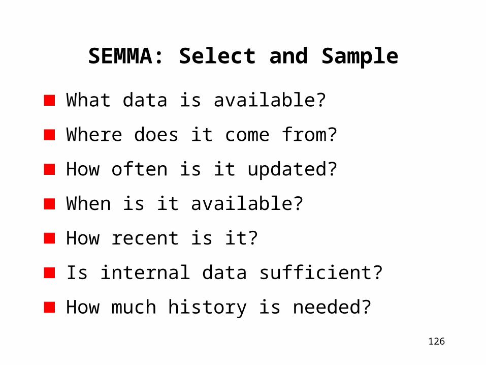
SEMMA: Select and Sample
What data is available?
Where does it come from?
How often is it updated?
When is it available?
How recent is it?
Is internal data sufficient?
How much history is needed?

127
Data Mining Prefers Customer Signatures
Often, the data come from many different sources
Relational database technology allows us to construct a customer signature from these multiple sources
The customer signature includes all the columns that describe a particular customer
the primary key is a customer idthe target columns contain the data we want to know more about (e.g., predict)the other columns are input columns
128
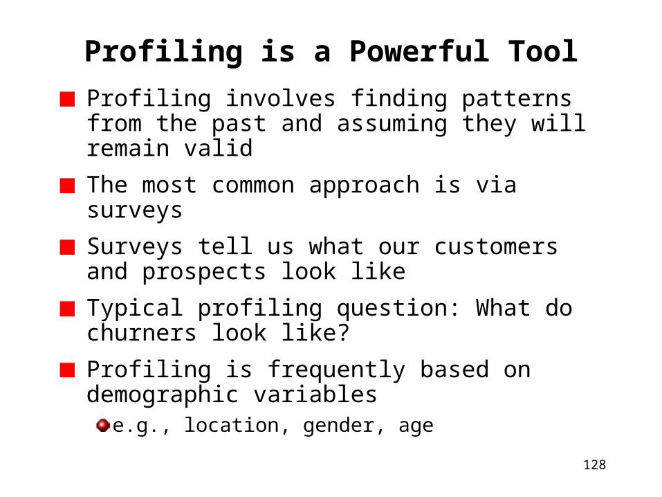
Profiling is a Powerful Tool
Profiling involves finding patterns from the past and assuming they will remain valid
The most common approach is via surveys
Surveys tell us what our customers and prospects look like
Typical profiling question: What do churners look like?
Profiling is frequently based on demographic variables
e.g., location, gender, age
129
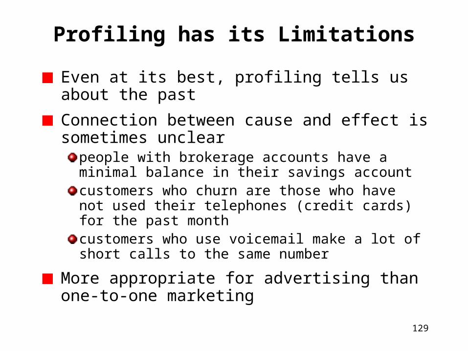
Profiling has its Limitations
Even at its best, profiling tells us about the past
Connection between cause and effect is sometimes unclear
people with brokerage accounts have a minimal balance in their savings accountcustomers who churn are those who have not used their telephones (credit cards) for the past monthcustomers who use voicemail make a lot of short calls to the same number
More appropriate for advertising than one-to-one marketing
130
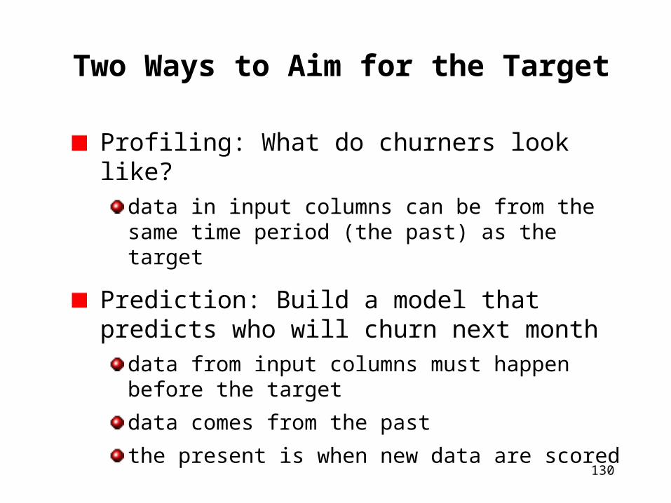
Two Ways to Aim for the Target
Profiling: What do churners look like?data in input columns can be from the same time period (the past) as the target
Prediction: Build a model that predicts who will churn next month
data from input columns must happen before the target
data comes from the past
the present is when new data are scored
131
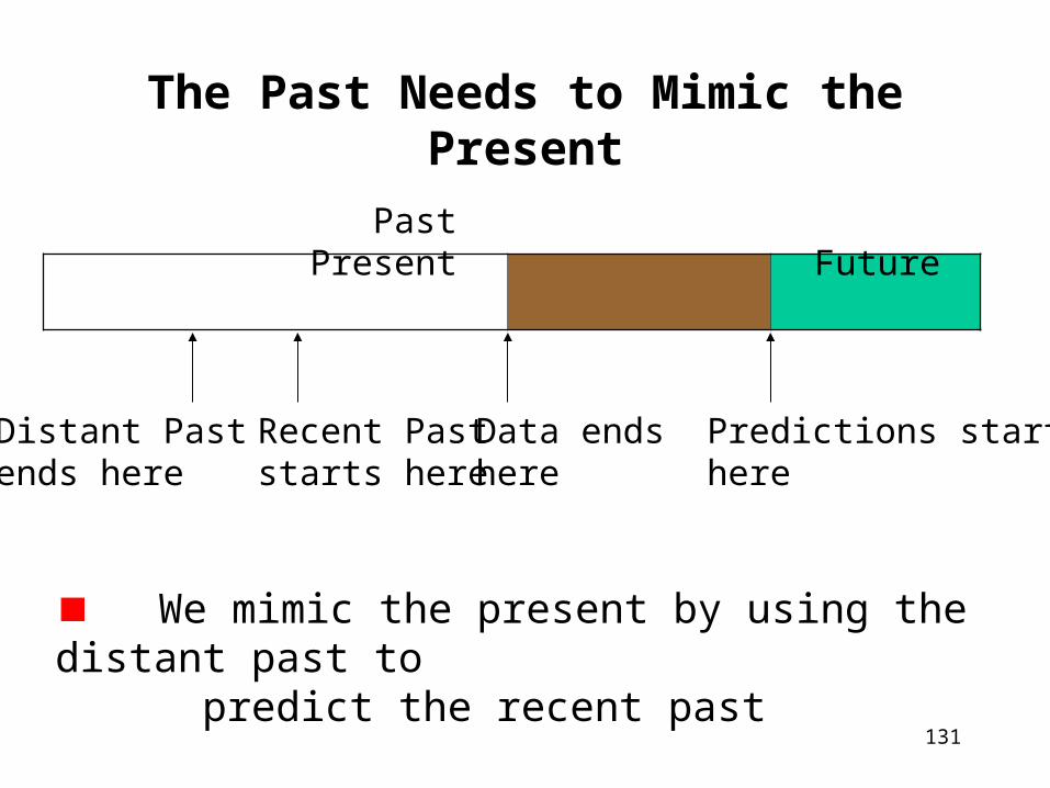
The Past Needs to Mimic the Present
Past Present Future
Distant Pastends here
Recent Paststarts here
Data endshere
Predictions starthere
We mimic the present by using the distant past to predict the recent past
132
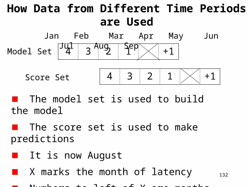
How Data from Different Time Periods are Used
4 3 2 1 +1
Jan Feb Mar Apr May Jun Jul Aug Sep
4 3 2 1 +1
Model Set
Score Set
The model set is used to build the model
The score set is used to make predictions
It is now August
X marks the month of latency
Numbers to left of X are months in the past
133
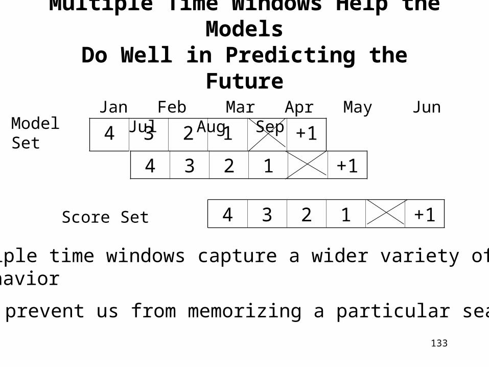
Multiple Time Windows Help the ModelsDo Well in Predicting the Future
4 3 2 1 +1
4 3 2 1 +1
Jan Feb Mar Apr May Jun Jul Aug SepModel Set
Score Set 4 3 2 1 +1
Multiple time windows capture a wider variety of past behavior
They prevent us from memorizing a particular season

134
Rules for Building a Model Set fora Prediction
All input columns must come strictly before the target
There should be a period of “latency” corresponding to the time needed to gather the data
The model set should contain multiple time windows of data
135
More about the Model and Score Sets
The model set can be partitioned into three subsetsthe model is trained using pre-classified data called the training set
the model is refined, in order to prevent memorization, using the test set
the performance of models can be compared using a third subset called the evaluation or validation set
The model is applied to the score set to predict the (unknown) future
136
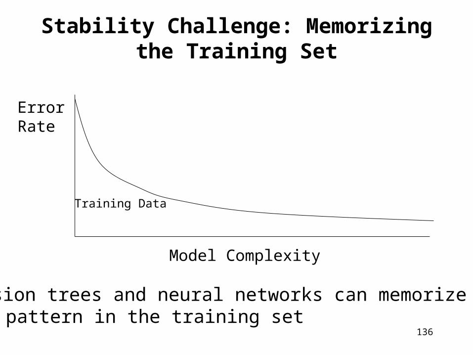
Stability Challenge: Memorizingthe Training Set
Training Data
ErrorRate
Model Complexity
Decision trees and neural networks can memorize nearly any pattern in the training set

137
Danger: OverfittingDanger: Overfitting
The model has overfit the training data
As model complexity grows, performance deteriorates on test data
Model Complexity
Training Data
Test Data
This is the model we wantError
Rate
138
Building the Model from Data
Both the training set and the test set are used to create the model
Algorithms find all the patterns in the training setsome patterns are global (should be true on unseen data)
some patterns are local (only found in the training set)
We use the test set to distinguish between the global patterns and the local patterns
Finally, the validation set is needed to evaluate the model’s performance
139
SEMMA: Explore the Data
Look at the range and distribution of all the variables
Identify outliers and most common values
Use histograms, scatter plots, and subsets
Use algorithms such as clustering and market basket analysis
Clementine does some of this for you when you load the data

140
SEMMA: Modify
Add derived variablestotal, percentages, normalized ranges, and so on
extract features from strings and codes
Add derived summary variablesmedian income in ZIP code
Remove unique, highly skewed, and correlated variables
often replacing them with derived variables
Modify the model set
141
The Density Problem
The model set contains a target variable“fraud” vs. “not fraud”“churn” vs. “still a customer”
Often binary, but not always
The density is the proportion of records with the given property (often quite low)
fraud ≈ 1%churn ≈ 5%
Predicting the common outcome is accurate, but not helpful
142
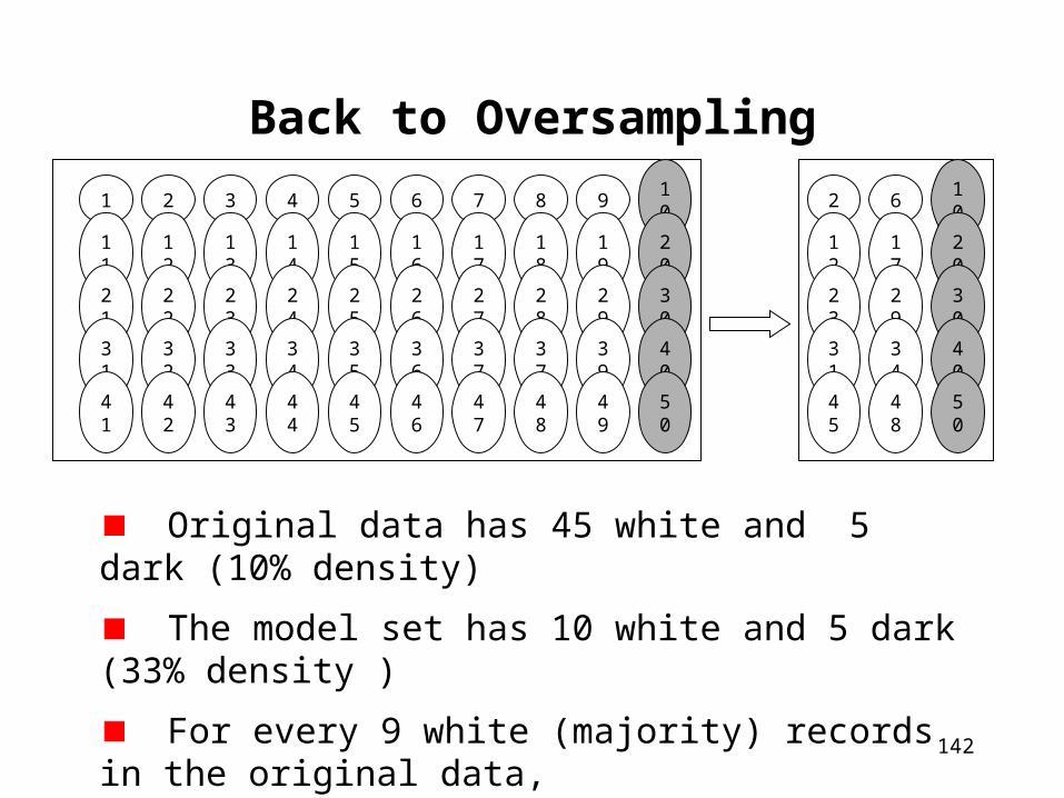
Back to Oversampling
Original data has 45 white and 5 dark (10% density)
The model set has 10 white and 5 dark (33% density )
For every 9 white (majority) records in the original data, two are in the oversampled model set
Oversampling rate is 9/2 = 4.5
1
11
21
31
41
2
12
22
32
42
3
13
23
33
43
4
14
24
34
44
5
15
25
35
45
6
16
26
36
46
7
17
27
37
47
8
18
28
37
48
9
19
29
39
49
10
20
30
40
50
10
20
30
40
50
2 6
12
17
23
29
31
34
45
48
143
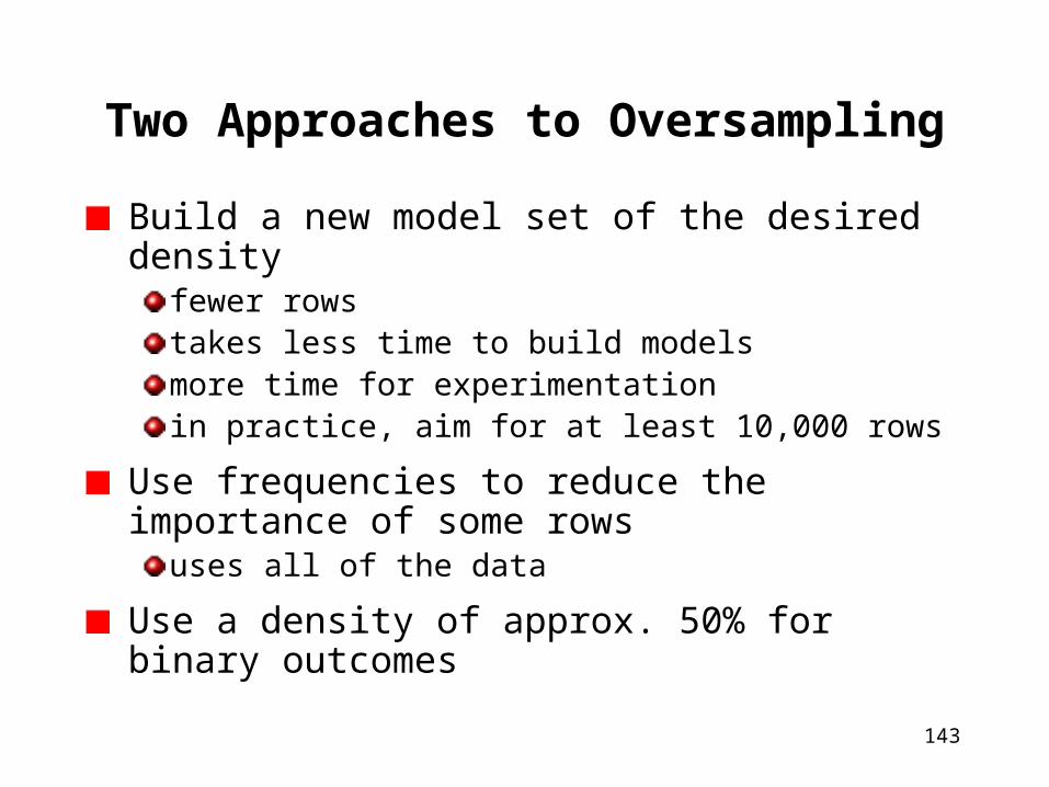
Two Approaches to Oversampling
Build a new model set of the desired densityfewer rowstakes less time to build modelsmore time for experimentationin practice, aim for at least 10,000 rows
Use frequencies to reduce the importance of some rows
uses all of the data
Use a density of approx. 50% for binary outcomes

144
Oversampling by Taking a Subset ofthe Model Set
ID Name State Flag
1 0102 Will MA F
2 0104 Sue NY F
3 0105 John AZ F
4 0110 Lori AZ F
5 0111 Beth NM T
6 0112 Pat WY F
7 0116 David ID F
8 0117 Frank MS T
9 0118 Ethel NE F
ID Name State Flag
1 0102 Will MA F
3 0105 John AZ F
5 0111 Beth NM T
6 0112 Pat WY F
8 0117 Frank MS T
9 0118 Ethel NE F
The original data has 2 Ts and 7 Fs (22% density)
Take all the Ts and 4 of the Fs (33% density)
The oversampling rate is 7/4 = 1.75
145
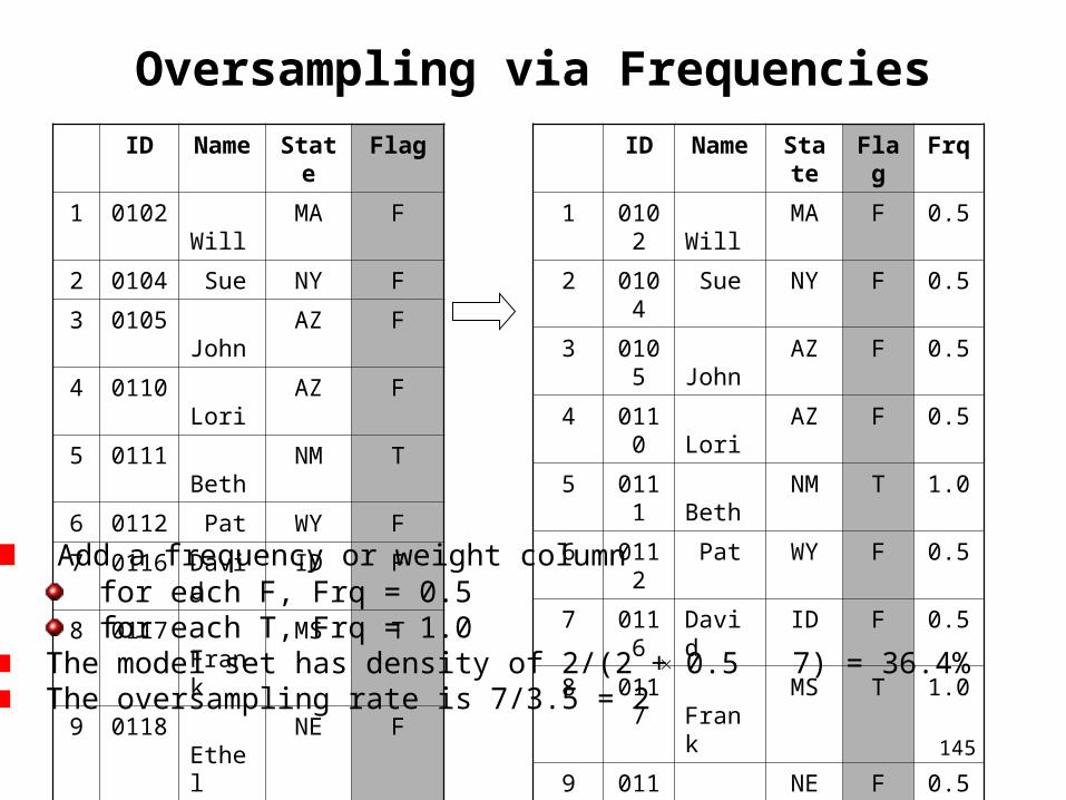
Oversampling via Frequencies
ID Name State Flag
1 0102 Will MA F
2 0104 Sue NY F
3 0105 John AZ F
4 0110 Lori AZ F
5 0111 Beth NM T
6 0112 Pat WY F
7 0116 David ID F
8 0117 Frank MS T
9 0118 Ethel NE F
ID Name State Flag Frq
1 0102 Will MA F 0.5
2 0104 Sue NY F 0.5
3 0105 John AZ F 0.5
4 0110 Lori AZ F 0.5
5 0111 Beth NM T 1.0
6 0112 Pat WY F 0.5
7 0116 David ID F 0.5
8 0117 Frank MS T 1.0
9 0118 Ethel NE F 0.5
Add a frequency or weight column for each F, Frq = 0.5 for each T, Frq = 1.0
The model set has density of 2/(2 + 0.5 7) = 36.4% The oversampling rate is 7/3.5 = 2
146
SEMMA: Model
Choose an appropriate technique decision trees
neural networks
regression
combination of above
Set parameters
Combine models

147
Regression
Tries to fit data points to a known curve
(often a straight line)
Standard (well-understood) statistical technique
Not a universal approximator (form of the regression needs to be specified in advance)
148
Neural Networks
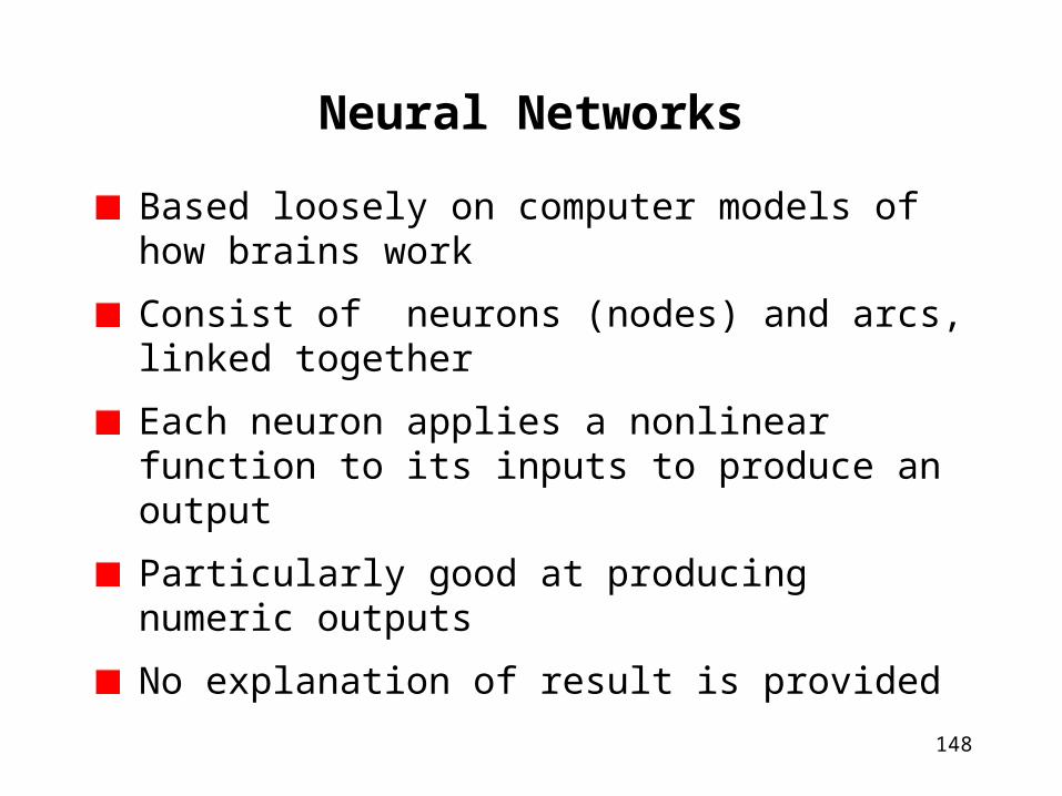
Based loosely on computer models of how brains work
Consist of neurons (nodes) and arcs, linked together
Each neuron applies a nonlinear function to its inputs to produce an output
Particularly good at producing numeric outputs
No explanation of result is provided

149
Decision Trees
Looks like a game of “Twenty Questions”
At each node, we fork based on variablese.g., is household income less than $40,000?
These nodes and forks form a tree
Decision trees are useful for classification problems
especially with two outcomes
Decision trees explain their resultthe most important variables are revealed

150
Experiment to Find the Best Modelfor Your Data
Try different modeling techniques
Try oversampling at different rates
Tweak the parameters
Add derived variables
Remember to focus on the business problem
151
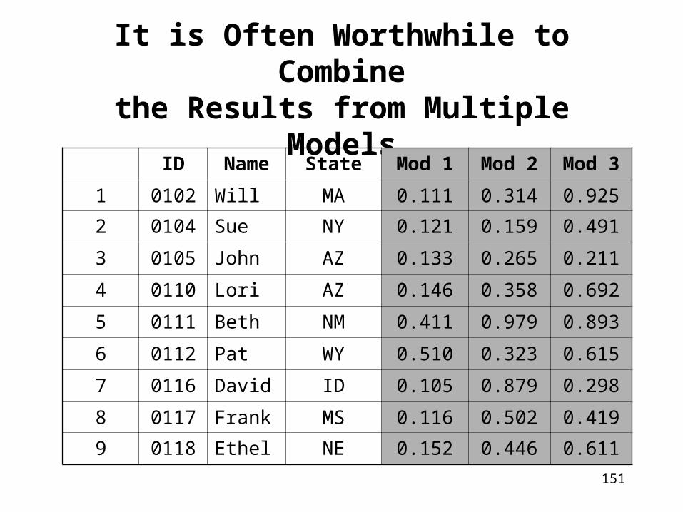
It is Often Worthwhile to Combinethe Results from Multiple Models
ID Name State Mod 1 Mod 2 Mod 3
1 0102 Will MA 0.111 0.314 0.925
2 0104 Sue NY 0.121 0.159 0.491
3 0105 John AZ 0.133 0.265 0.211
4 0110 Lori AZ 0.146 0.358 0.692
5 0111 Beth NM 0.411 0.979 0.893
6 0112 Pat WY 0.510 0.323 0.615
7 0116 David ID 0.105 0.879 0.298
8 0117 Frank MS 0.116 0.502 0.419
9 0118 Ethel NE 0.152 0.446 0.611
152
Multiple-Model Voting
Multiple models are built using the same input data
Then a vote, often a simple majority or plurality rules vote, is used for the final classification
Requires that models be compatible
Tends to be robust and can return better results
153
Segmented Input Models
Segment the input databy customer segment
by recency
Build a separate model for each segment
Requires that model results be compatible
Allows different models to focus and different models to use richer data

154
Combining Models
What is response to a mailing from a non-profit raising money (1998 data set)
Exploring the data revealedthe more often, the less money one contributes each time
so, best customers are not always most frequent
Thus, two models were developedwho will respond?
how much will they give?

155
Compatible Model Results
In general, the score refers to a probabilityfor decision trees, the score may be the actual density of a leaf node
for a neural network, the score may be interpreted as the probability of an outcome
However, the probability depends on the density of the model set
The density of the model set depends on the oversampling rate

156
An Example
The original data has 10% density
The model set has 33% density
Each white in model set represents 4.5 white in original data
Each dark represents one dark
The oversampling rate is 4.5

157
A Score Represents a Portion of the Model Set
Suppose an algorithm identifies the
group at right as most likely to churn
The score would be 4/6 = 67%,
versus the density of 33% for the
entire model set
This score represents the probability
on the oversampled data
This group has a lift of 67/33 = 2
158
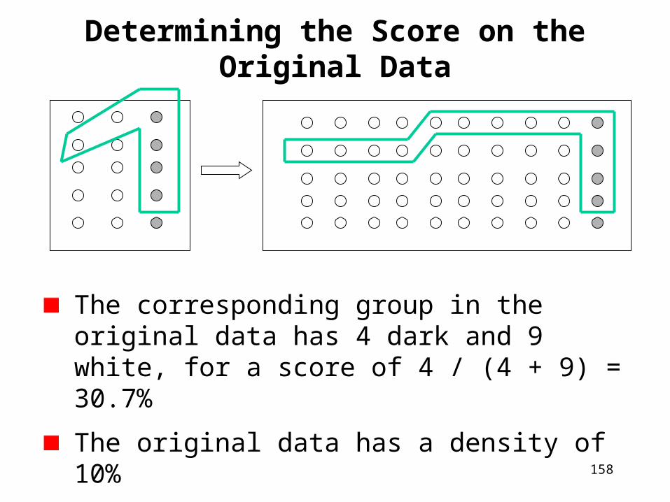
Determining the Score on the Original Data
The corresponding group in the original data has 4 dark and 9 white, for a score of 4 / (4 + 9) = 30.7%
The original data has a density of 10%
The lift is now 30.7/10 = 3.07
159
Determining the Score -- continued
The original group accounted for 6/15 = 40% of the model set
In the original data, it corresponds to 13/50 = 26%
Bottom line: before comparing the scores that different models produce, make sure that these scores are adjusted for the oversampling rate
The final part of the SEMMA process is to assess the results

160
Confusion Matrix (or Correct Classification Matrix)
When the model predicts No, it is right 100/150 = 67% of the time
The density of the model set is 150/1000 = 15%
There are 1000 records in the model set
When the model predicts Yes, it is right 800/850 = 94% of the time
Yes No
800 50
50 100
Yes
NoPre
dict
ed
Actual

161
Confusion Matrix-- continued
The model is correct 800 times in predicting Yes
The model is correct 100 times in predicting No
The model is wrong 100 times in total
The overall prediction accuracy is
900/1000 = 90%
162
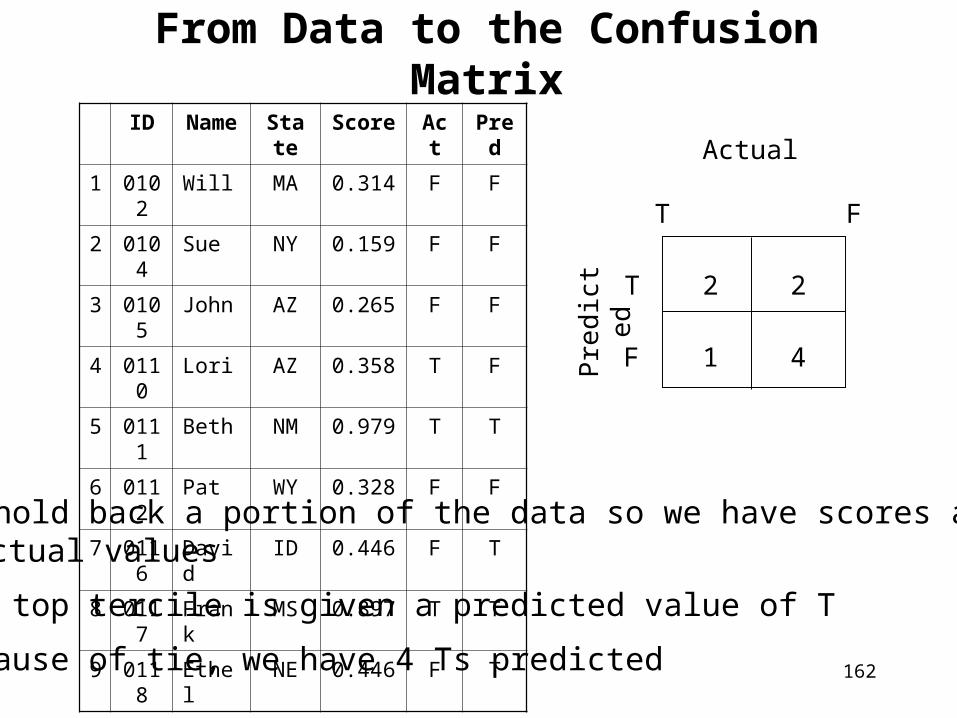
From Data to the Confusion Matrix
T F
2 2
1 4
T
FPre
dict
ed
ID Name State Score Act Pred
1 0102 Will MA 0.314 F F
2 0104 Sue NY 0.159 F F
3 0105 John AZ 0.265 F F
4 0110 Lori AZ 0.358 T F
5 0111 Beth NM 0.979 T T
6 0112 Pat WY 0.328 F F
7 0116 David ID 0.446 F T
8 0117 Frank MS 0.897 T T
9 0118 Ethel NE 0.446 F T
Actual
We hold back a portion of the data so we have scores and actual values
The top tercile is given a predicted value of T
Because of tie, we have 4 Ts predicted

163
How Oversampling Affects the Results
The model set has a density of 15% No
Suppose we achieve this density with an oversampling rate of 10
So, for every Yes in the model set there are 10 Yes’s in the original data
Yes No
800 50
50 100
Yes
No
Pre
dict
ed
Actual Yes No
8000 50
500 100
Yes
NoPre
dict
ed
Actual
Model set Original data
164
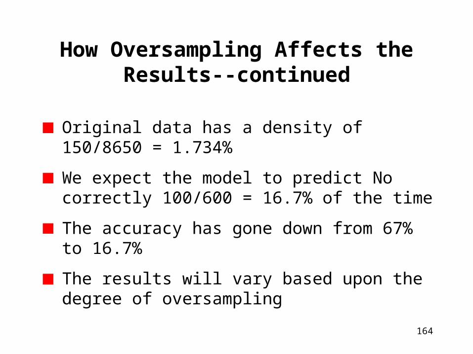
How Oversampling Affects the Results--continued
Original data has a density of 150/8650 = 1.734%
We expect the model to predict No correctly 100/600 = 16.7% of the time
The accuracy has gone down from 67% to 16.7%
The results will vary based upon the degree of oversampling
165
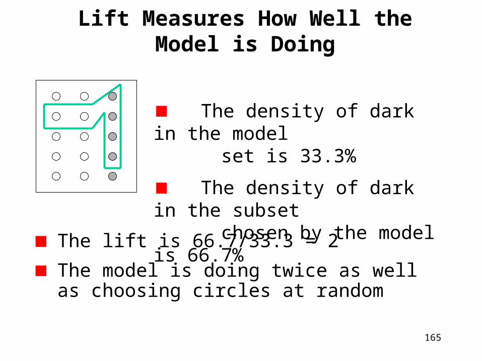
Lift Measures How Well the Model is Doing
The lift is 66.7/33.3 = 2
The model is doing twice as well as choosing circles at random
The density of dark in the model set is 33.3%
The density of dark in the subset chosen by the model is 66.7%
166
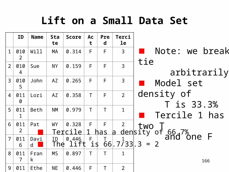
Lift on a Small Data Set
Tercile 1 has a density of 66.7%
The lift is 66.7/33.3 = 2
ID Name State Score Act Pred Tercile
1 0102 Will MA 0.314 F F 3
2 0104 Sue NY 0.159 F F 3
3 0105 John AZ 0.265 F F 3
4 0110 Lori AZ 0.358 T F 2
5 0111 Beth NM 0.979 T T 1
6 0112 Pat WY 0.328 F F 2
7 0116 David ID 0.446 F T 1
8 0117 Frank MS 0.897 T T 1
9 0118 Ethel NE 0.446 F T 2
Note: we break tie arbitrarily
Model set density of T is 33.3%
Tercile 1 has two T and one F
167
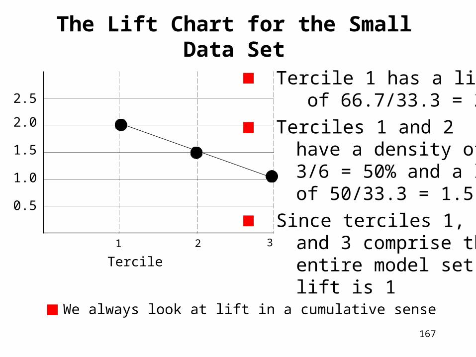
The Lift Chart for the Small Data Set
We always look at lift in a cumulative sense
1 2 3
Tercile 1 has a lift of 66.7/33.3 = 2
Terciles 1 and 2 have a density of 3/6 = 50% and a lift of 50/33.3 = 1.5
Since terciles 1, 2, and 3 comprise the entire model set, the lift is 1
2.5
2.0
1.5
1.0
0.5
Tercile
168
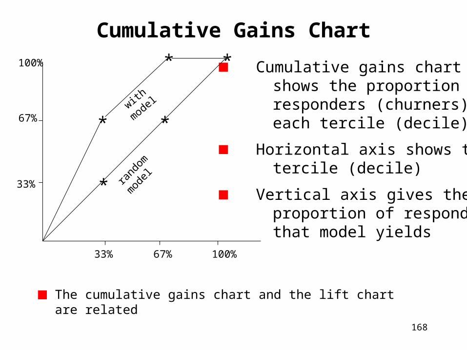
Cumulative Gains Chart
The cumulative gains chart and the lift chart are related
100%
67%
33%
33% 67% 100%
with m
odel
rando
m mod
el
Cumulative gains chart shows the proportion of responders (churners) in each tercile (decile)
Horizontal axis shows the tercile (decile)
Vertical axis gives the proportion of responders that model yields
*
* *
*
*
169
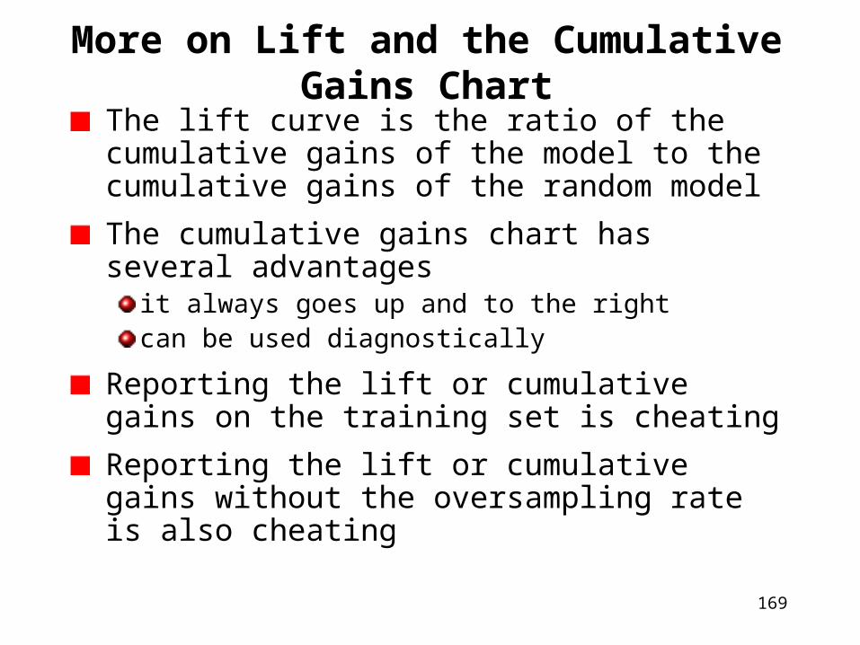
More on Lift and the Cumulative Gains Chart
The lift curve is the ratio of the cumulative gains of the model to the cumulative gains of the random model
The cumulative gains chart has several advantages
it always goes up and to the rightcan be used diagnostically
Reporting the lift or cumulative gains on the training set is cheating
Reporting the lift or cumulative gains without the oversampling rate is also cheating
170
Summary of Data Mining Process
Cycle of Data Miningidentify the right business problemtransform data into actionable informationact on the informationmeasure the effect
SEMMAselect/sample data to create the model setexplore the datamodify data as necessarymodel to produce resultsassess effectiveness of the models
171
The Data in Data Mining
Data comes in many formsinternal and external sources
Different sources of data have different peculiarities
Data mining algorithms rely on a customer signature
one row per customer
multiple columns
See Chapter 6 in Mastering Data Mining for details
172
Preventing Customer Attrition
We use the noun churn as a synonym for attrition
We use the verb churn as a synonym for leave
Why study attrition?it is a well-defined problem
it has a clear business value
we know our customers and which ones are valuable
we can rely on internal data
the problem is well-suited to predictive modeling

173
When You Know Who is Likely to Leave,You Can …
Focus on keeping high-value customers
Focus on keeping high-potential customers
Allow low-potential customers to leave, especially if they are costing money
Don’t intervene in every case
Topic should be called “managing customer attrition”
174
The Challenge of Defining Customer Value
We know how customers behaved in the past
We know how similar customers behaved in the past
Customers have control over revenues, but much less control over costs
we may prefer to focus on net revenue rather than profit
We can use all of this information to estimate customer worth
These estimates make sense for the near future
175
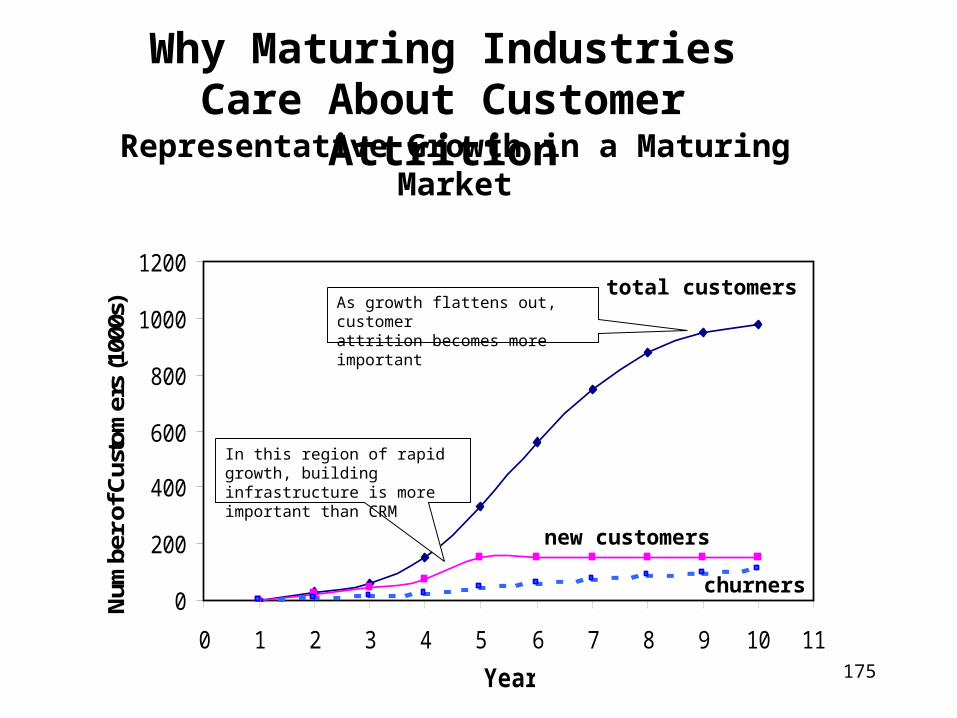
Representative Growth in a Maturing Market
Why Maturing Industries Care About Customer Attrition
0
200
400
600
800
1000
1200
0 1 2 3 4 5 6 7 8 9 10 11
Year
Num
ber
of C
usto
mer
s (1
000s
) As growth flattens out, customerattrition becomes more important
In this region of rapid growth, building infrastructure is more important than CRM
total customers
new customers
churners
176
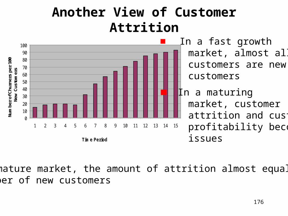
Another View of Customer Attrition
0
10
20
30
40
50
60
70
80
90
100
1 2 3 4 5 6 7 8 9 10 11 12 13 14 15
Time Period
Num
ber
of C
hurn
ers
per
100
New
Cus
tom
ers
In a fast growth market, almost all customers are new customers
In a maturing market, customer attrition and customer profitability become issues
In a mature market, the amount of attrition almost equals the number of new customers
177
Why Attrition is Important
When markets are growing rapidly, attrition is usually not important
customer acquisition is more important
Eventually, every new customer is simply replacing one who left
Before this point, it is cheaper to prevent attrition than to spend money on customer acquisition
One reason is that, as a market becomes saturated, acquisition costs go up

178
$0
$50
$100
$150
$200
$250
0.00% 1.00% 2.00% 3.00% 4.00% 5.00% 6.00%
Response Rate
Cos
t per
Res
pons
eIn Maturing Markets, Acquisition Response
Rates Decrease and Costs Increase
Assumption: $1 per contact,$20 offer
220
120
7053.3
45 40

179
$0
$50
$100
$150
$200
$250
0.00% 1.00% 2.00% 3.00% 4.00% 5.00% 6.00%
Response Rate
Cos
t per
Res
pons
eAcquisition versus Retention
Assumption: $1 per contact,$20 offer
220
120
7053.3
45 40

180
Acquisition versus Retention-- continued
As response rate drops, suppose we spend $140 to obtain a new customer
Alternatively, we could spend $140 to retain an existing customer
Assume the two customers have the same potential value
Some possible optionsdecrease the costs of the acquisition campaign
implement a customer retention campaign
combination of both
181
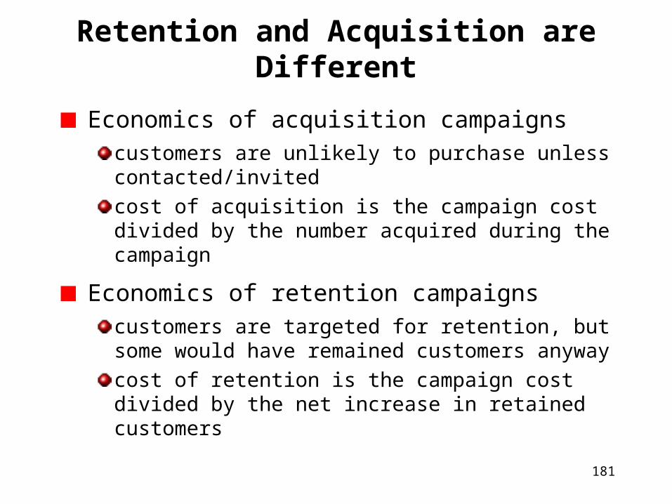
Retention and Acquisition are Different
Economics of acquisition campaignscustomers are unlikely to purchase unless contacted/invited
cost of acquisition is the campaign cost divided by the number acquired during the campaign
Economics of retention campaignscustomers are targeted for retention, but some would have remained customers anyway
cost of retention is the campaign cost divided by the net increase in retained customers

182
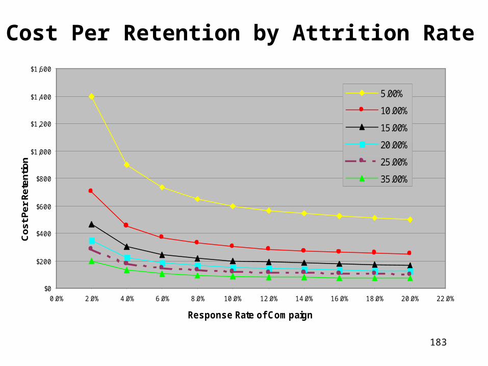
Cost per Retention: How ManyResponders Would Have Left?
For a retention campaign, we need to distinguish between customers who merely respond and those who respond and would have left
If the overall group has an attrition rate of 25%, you can assume that one quarter of the responders are saved
Since people like to receive something for nothing, response rates tend to be high
As before, assume $1 per contact and $20 per response
We need to specify response rate and attrition rate
183
Cost Per Retention by Attrition Rate
$0
$200
$400
$600
$800
$1,000
$1,200
$1,400
$1,600
0.0% 2.0% 4.0% 6.0% 8.0% 10.0% 12.0% 14.0% 16.0% 18.0% 20.0% 22.0%
Response Rate of Compaign
Co
st
Pe
r R
ete
nti
on
5.00%
10.00%
15.00%
20.00%
25.00%
35.00%
184
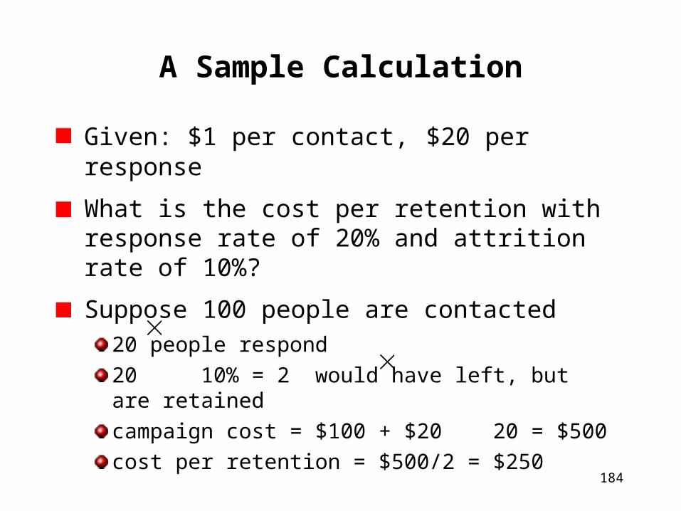
A Sample Calculation
Given: $1 per contact, $20 per response
What is the cost per retention with response rate of 20% and attrition rate of 10%?
Suppose 100 people are contacted20 people respond
20 10% = 2 would have left, but are retained
campaign cost = $100 + $20 20 = $500
cost per retention = $500/2 = $250
185
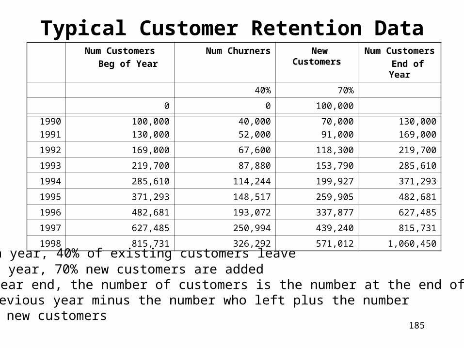
Typical Customer Retention DataNum Customers
Beg of Year
Num Churners New Customers Num Customers
End of Year
40% 70%
0 0 100,000
1990
1991
100,000
130,000
40,000
52,000
70,000
91,000
130,000
169,000
1992 169,000 67,600 118,300 219,700
1993 219,700 87,880 153,790 285,610
1994 285,610 114,244 199,927 371,293
1995 371,293 148,517 259,905 482,681
1996 482,681 193,072 337,877 627,485
1997 627,485 250,994 439,240 815,731
1998 815,731 326,292 571,012 1,060,450
Each year, 40% of existing customers leave Each year, 70% new customers are added At year end, the number of customers is the number at the end of the
previous year minus the number who left plus the number of new customers

186
How to Lie with Statistics
Num Customers
Beg of Year
Num Churners New Customers
Num Customers
End of Year
Reported Churn
40% 70%
0 0 100,000 0
1990
1991
100,000
130,000
40,000
52,000
70,000
91,000
130,000
169,000
30.77%
30.77%
1992 169,000 67,600 118,300 219,700 30.77%
1993 219,700 87,880 153,790 285,610 30.77%
1994 285,610 114,244 199,927 371,293 30.77%
1995 371,293 148,517 259,905 482,681 30.77%
1996 482,681 193,072 337,877 627,485 30.77%
1997 627,485 250,994 439,240 815,731 30.77%
1998 815,731 326,292 571,012 1,060,450 30.77%
When we divide by end-of-year customers, we reduce the attrition rate to about 31% per year
This may look better, but it is cheating

187
Suppose Acquisition Suddenly Stops
Num Customers
Beg of Year
Num Churners New Customers Num Customers
End of Year
Reported Churn
40% 70%
0 0 100,000 0
1990
1991
100,000
130,000
40,000
52,000
70,000
91,000
130,000
169,000
30.77%
30.77%
1992 169,000 67,600 118,300 219,700 30.77%
1993 219,700 87,880 153,790 285,610 30.77%
1994 285,610 114,244 199,927 371,293 30.77%
1995 371,293 148,517 259,905 482,681 30.77%
1996 482,681 193,072 337,877 627,485 30.77%
1997 627,485 250,994 439,240 815,731 30.77%
1998
1999
815,731
1,060,450
326,292
424,180
571,012
0
1,060,450
636,270
30.77%
66.67%
If acquisition of new customers stops, existing customers still leave at same rate
But, churn rate more than doubles

188
Measuring Attrition the Right Wayis Difficult
The “right way” gives a value of 40% instead of 30.77%
who wants to increase their attrition rate?
this happens when the number of customers is increasing
For our small example, we assume that new customers do not leave during their first year
the real world is more complicated
we might look at the number of customers on a monthly basis

189
-$5,000,000
$0
$5,000,000
$10,000,000
$15,000,000
$20,000,000
$25,000,000
90 91 92 93 94 95 96 97 98
N e w C u s t o m e r R e v e n u e
E x i s t i n g C u s t o m e r R e v e n u e
L o s s D u e t o A t t r i t i o n
Assumption: $20 for existing customers;
$10 for new customers
Rev
enu
e
Time
Effect of Attrition on Revenue
Effect of Attrition on Revenue
190
Effect of Attrition on Revenues -- continued
From previous page, the loss due to attrition is about the same as the new customers revenue
The loss due to attrition has a cumulative impact
If we could retain some of these customers each year, they would generate revenue well into the future
It is useful to examine the relationship between attrition and the length of the customer relationship
Often, attrition is greater for longer-duration customers
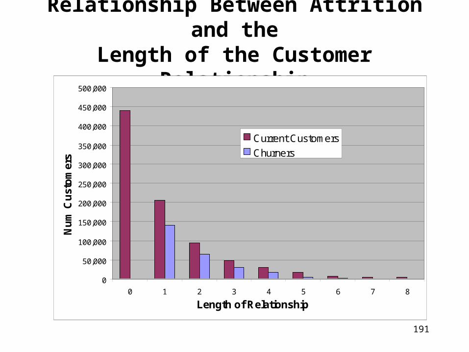
191
Relationship Between Attrition and theLength of the Customer Relationship
0
50,000
100,000
150,000
200,000
250,000
300,000
350,000
400,000
450,000
500,000
0 1 2 3 4 5 6 7 8
Length of Relationship
Nu
m C
ust
om
ers
Current Customers
Churners

192
What is a Customer Attrition Score?
When building an attrition model, we seek a score for each customer
This adds a new column to the data
Two common approachesa relative score or ranking of who is going to leave
an estimate of the likelihood of leaving in the next time period

193
Attrition Scores are an ImportantPart of the Solution
Having an idea about which customers will leave does not address key business issues
why are they leaving?
where are they going?
is brand strength weakening?
are the products still competitive?
However, it does allow for more targeted marketing to customers
it is often possible to gain understanding and combat attrition while using attrition models

194
Requirements of Effective Attrition Management
Keeping track of the attrition rate over time
Understanding how different methods of acquisition impact attrition
Looking at some measure of customer value, to determine which customers to let leave
Implementing attrition retention efforts for high-value customers
Knowing who might leave in the near future
195
Three Types of AttritionVoluntary attrition
when the customer goes to a competitorour primary focus is on voluntary attrition models
Forced attritionwhen the company decides that it no longer wants the customer and cancels the accountoften due to non-paymentour secondary focus is on forced attrition models
Expected attritionwhen the customer changes lifestyle and no longer needs your product or service
196
What is Attrition?
In the telecommunications industry it is very clearcustomers pay each month for service
customers must explicitly cancel service
the customer relationship is primarily built around a single product
It is not so clear in other industriesretail banking
credit cards
retail
e-commerce
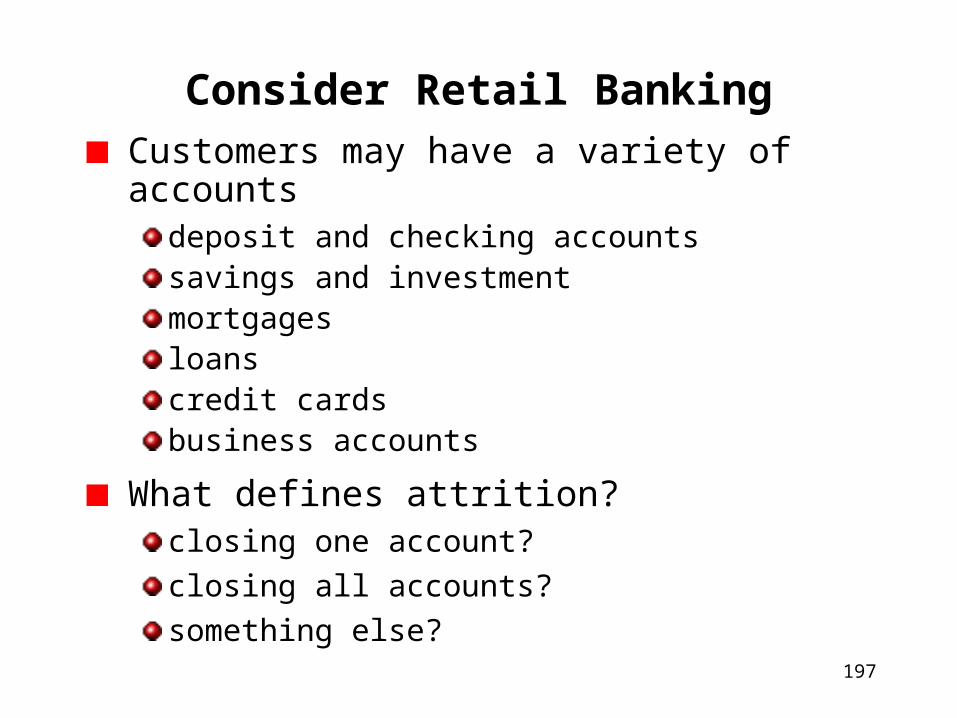
197
Consider Retail Banking
Customers may have a variety of accountsdeposit and checking accountssavings and investmentmortgagesloanscredit cardsbusiness accounts
What defines attrition?closing one account?
closing all accounts?
something else?

198
Retail Banking--Continued
One large bank uses checking account balance to define churn
What if a customer (e.g., credit card or mortgage customer) does not have a checking account with the bank?
Another example from retail banking involves forced attrition
Consider the bank loan timeline on the next page
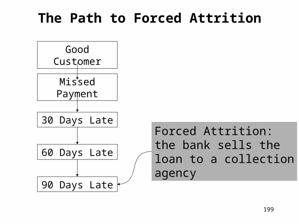
199
The Path to Forced Attrition
Forced Attrition:the bank sells the loan to a collectionagency
Good Customer
90 Days Late
Missed Payment
30 Days Late
60 Days Late

200
Credit CardsCredit cards, in the U.S., typically don’t have an annual fee
there is no incentive for a cardholder to tell you when she no longer plans on using the card
Cardholders typically use the card several times each month
Customers who stop using the card and are not carrying a balance are considered to be silent churners
The definition of silent churn varies among issuerscustomers who have not used the card for six months
customers who have not used the card for three months and for nine of the last twelve months
201
The Catalog Industry
Like credit cards, catalogs are freetherefore, customers have little incentive to cancel them
Unlike credit cards, purchases from catalogs are more sporadic
so defining silent churn is more difficult
Purchases from catalogs are often seasonalso silent churn is measured over the course of years, rather than months
202
E-commerce
Attrition in e-commerce is hardest of all to defineconsider Amazon
Web sites are free, so there is no incentive to announce intention to churn
Customers often visit many times before making a purchase
Some customers buy frequently and others don’thow can Amazon decrease time between purchases?
The e-commerce world is still growing rapidly, so customer retention is not a major issue
But it will become a major issue soon
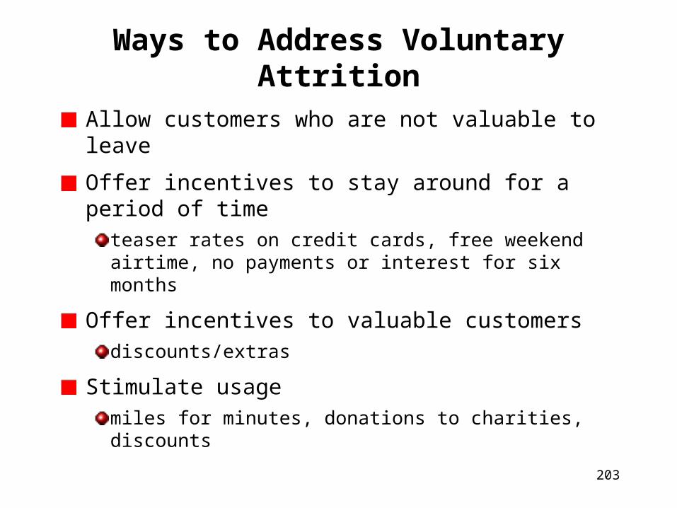
203
Ways to Address Voluntary Attrition
Allow customers who are not valuable to leave
Offer incentives to stay around for a period of timeteaser rates on credit cards, free weekend airtime, no payments or interest for six months
Offer incentives to valuable customersdiscounts/extras
Stimulate usagemiles for minutes, donations to charities, discounts

204
Predicting Voluntary Attrition Can Be Dangerous
Voluntary attrition sometimes looks like expected or forced attrition
Confusing voluntary and expected attrition results in the waste of marketing dollars
Confusing voluntary and forced attrition means you lose twice
by, again, wasting marketing dollars
by incurring customer non-payment

205
Ways to Address Forced Attrition
Stop marketing to the customerno more catalogs, billing inserts, or other usage stimulation
Reduce credit lines
Increase minimum payments
Accelerate cancellation timeline
Increase interest rates to increase customer value while he is still paying
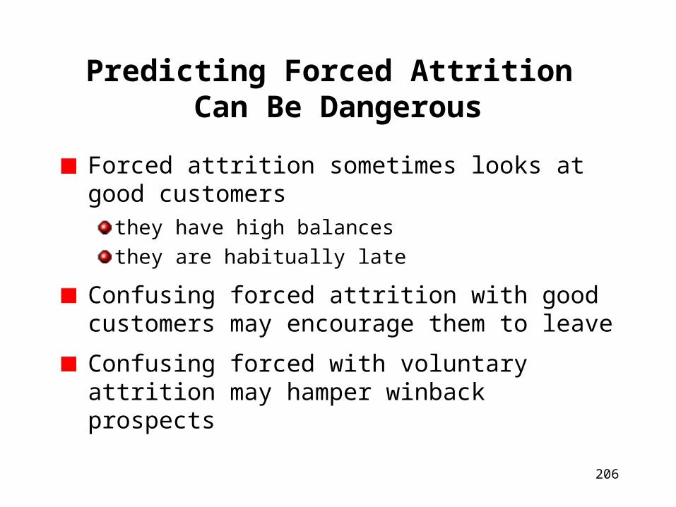
206
Predicting Forced Attrition Can Be Dangerous
Forced attrition sometimes looks at good customers
they have high balances
they are habitually late
Confusing forced attrition with good customers may encourage them to leave
Confusing forced with voluntary attrition may hamper winback prospects

207
Attrition Scores are Designed for theNear Future
The chance that someone will leave tomorrow is essentially 0%
The chance that someone will leave in the next 100 years is essentially 100%
A good attrition score is valid for one to three months in the future
Attrition modeling can take place at any point in the customer lifecycle
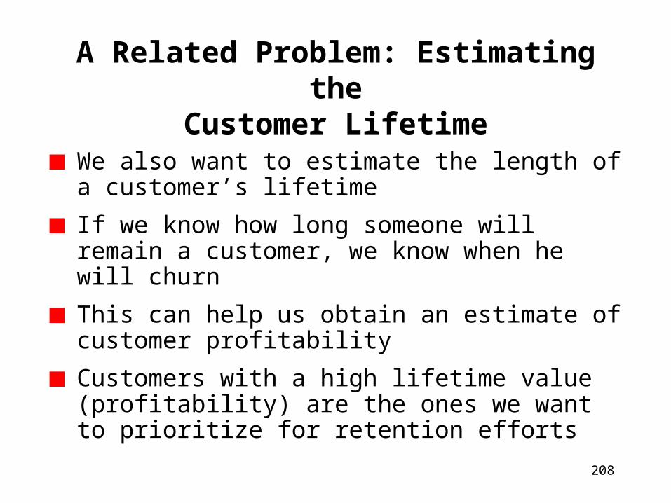
208
A Related Problem: Estimating theCustomer Lifetime
We also want to estimate the length of a customer’s lifetime
If we know how long someone will remain a customer, we know when he will churn
This can help us obtain an estimate of customer profitability
Customers with a high lifetime value (profitability) are the ones we want to prioritize for retention efforts
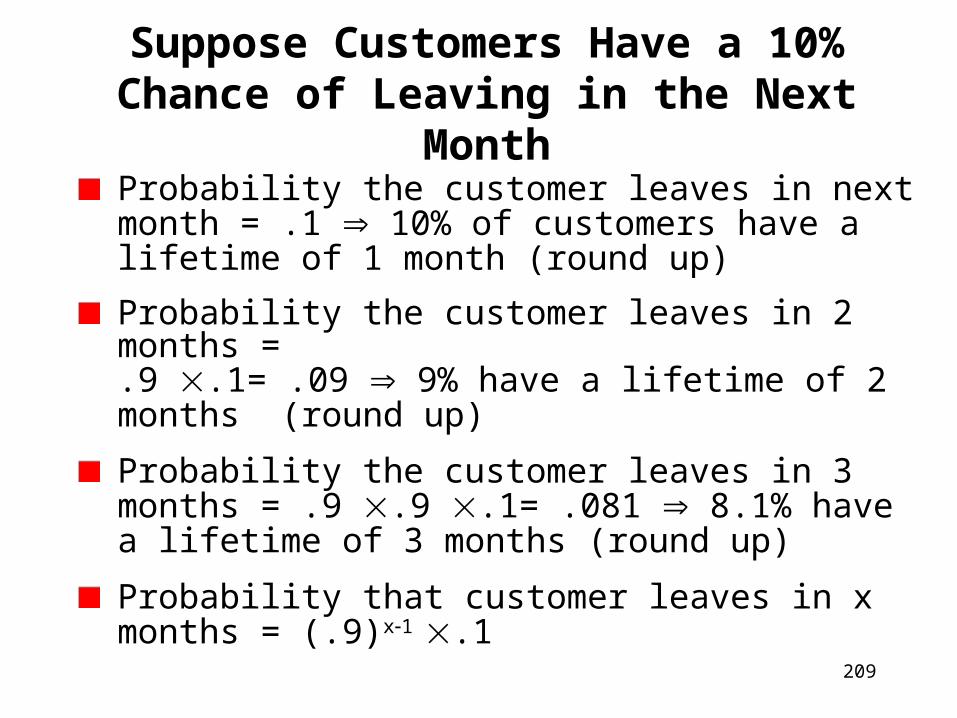
209
Suppose Customers Have a 10% Chance of Leaving in the Next Month
Probability the customer leaves in next month = .1 10% of customers have a lifetime of 1 month (round up)
Probability the customer leaves in 2 months = .9 .1= .09 9% have a lifetime of 2 months (round up)
Probability the customer leaves in 3 months = .9 .9 .1= .081 8.1% have a lifetime of 3 months (round up)
Probability that customer leaves in x months = (.9)x1
.1

210
Average Customer Lifetime
In statistics, we refer to this as a geometric distribution
If the churn rate per month is x%, the average lifetime is 1/x% months
In this example, the average lifetime is 1/.1= 10 months
An ideal attrition model says
all customers leaving in the next month get a score of 1 or 100%
all other customers get a score of 0 or 0%
211
Attrition Modeling Summary
It is very important to manage attrition, especially in maturing industries
Slowing attrition may be the cheapest way to maintain a critical mass of customers
There are different types of attrition
voluntary, forced, expected
Related to attrition is the customer lifetime
useful in calculating lifetime customer value
212
CRM Sources
The vast majority of these CRM slides has been borrowed, adapted, or reworked from one of the two sources below
1. Michael Berry and Gordon Linoff, CustomerRelationship Management Through Data Mining,
SAS Institute, 2000
2. Michael Berry and Gordon Linoff, Mastering Data Mining, John Wiley & Sons, 2000
I have also consulted Data Mining Techniques (Wiley, 1997) by Berry and Linoff, in preparing these slides

213
Decision Trees and Churn Modeling
Learn about decision treeswhat are they?
how are they built?
advantages versus disadvantages
Case study from the cellular telephone industryproblem definition
looking at the results
other techniques for modeling churn

214
Data Mining with Decision Trees
A decision tree is a set of rules represented in a tree structure
Easy to understand how predictions are made
Easy to build and visualize
Can be used for binary or multiple outcomes
Roots, nodes, leaves, and splits
215
Data Mining with Decision Trees--continued
We build the decision tree using the training and test sets
The decision tree allows us tomake predictionsunderstand why certain predictions make senseunderstand which variables are most importantspot unexpected patterns
There is one path from the root to any leaf
A given data record is associated with a single leaf
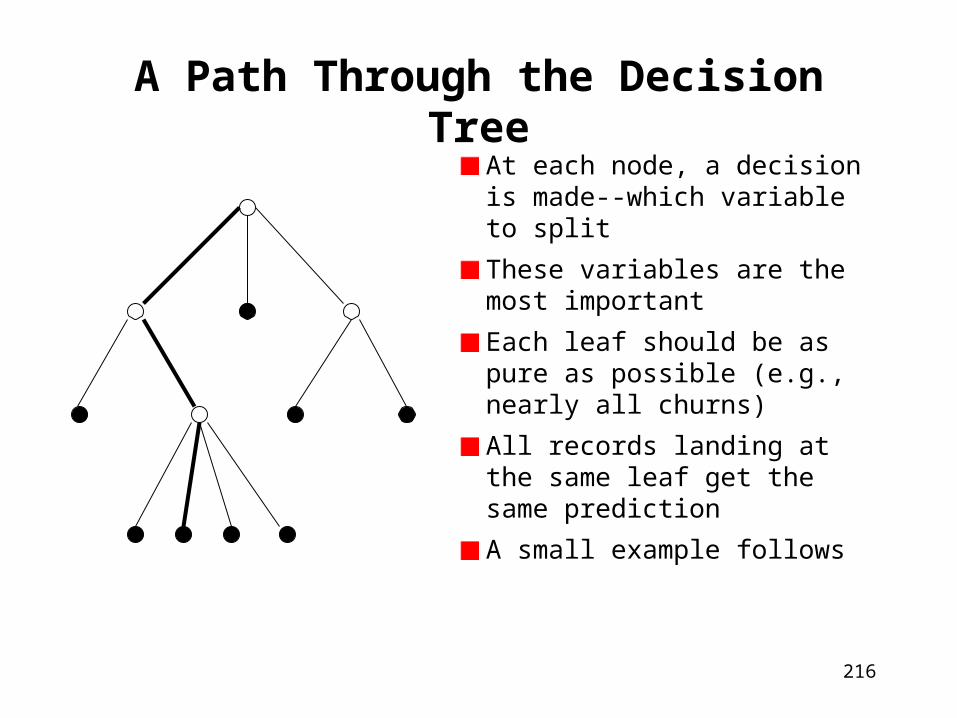
216
A Path Through the Decision Tree
At each node, a decision is made--which variable to split
These variables are the most important
Each leaf should be as pure as possible (e.g., nearly all churns)
All records landing at the same leaf get the same prediction
A small example follows
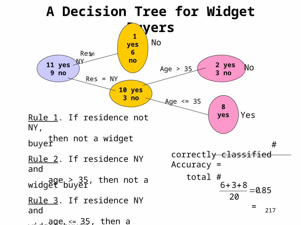
217
A Decision Tree for Widget Buyers
1 yes6 no
10 yes3 no
11 yes9 no
2 yes 3 no
8 yes
Res NY
Res = NY
Age > 35
Age <= 35
Rule 1. If residence not NY, then not a widget buyer
Rule 2. If residence NY and age > 35, then not a widget buyer
Rule 3. If residence NY and age <= 35, then a widget buyer
Adapted from (Dhar & Stein, 1997)
No
No
Yes
# correctly classifiedAccuracy = total #
= 85020
836.
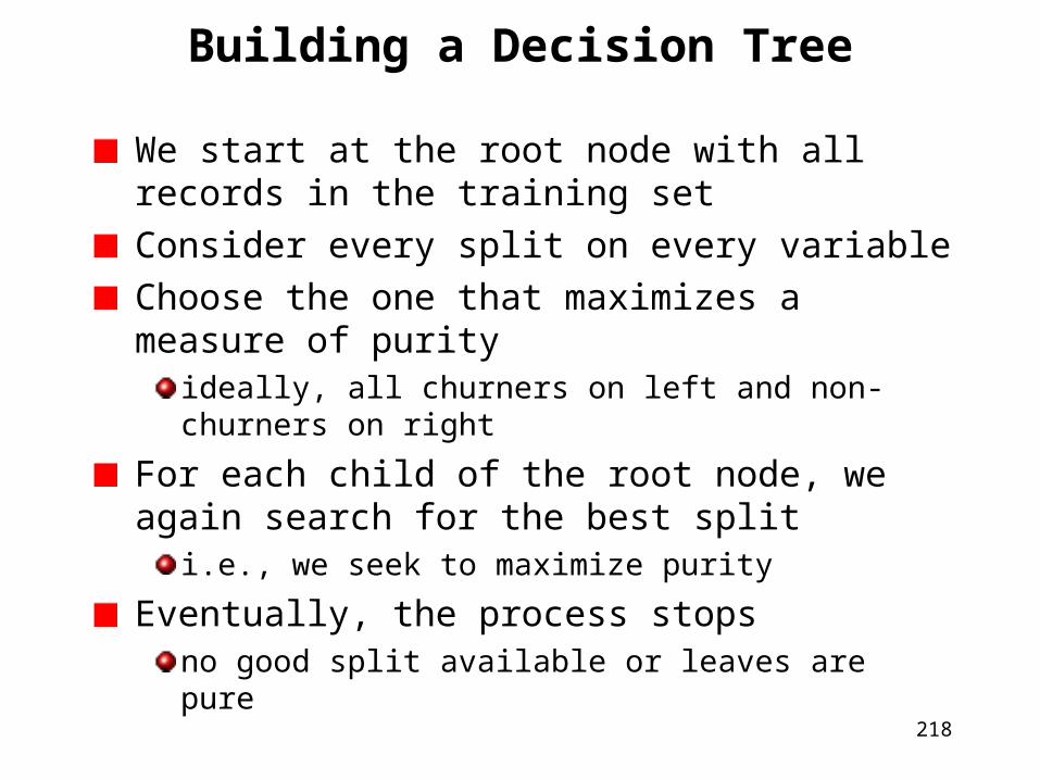
218
Building a Decision Tree
We start at the root node with all records in the training set
Consider every split on every variable
Choose the one that maximizes a measure of purity
ideally, all churners on left and non-churners on right
For each child of the root node, we again search for the best split
i.e., we seek to maximize purity
Eventually, the process stopsno good split available or leaves are pure
219
Building a Decision Tree--continued
The above process is sometimes called recursive partitioning
To avoid overfitting, we prune the tree using the test set
to prune is to simplify
After the tree has been built, each leaf node has a score
A leaf score may be the likelihood that the more common class arises
in training and test sets

220
The Leaves Contain the Scores
Overall, the most common class is No
11,112 records (including Sam’s) are associated with this leaf
96.5% are not fraudulent
Sam gets a score of .965Yes 3.5%
No 96.5%
Size 11,112

221
Scoring Using a Decision Tree
This example shows the relationship between records in a table and decision tree leaves
Remember, each record will fall in exactly one leaf
ID Name State Score
1 0102 Will MA 0.428
2 0112 Pat WY 0.283
3 0116 David ID 0.957
4 0117 Frank MS 0.892
5 0118 Ethel NE 0.957

222
A Real Life Example: Predicting Churn
Churn data from the cellular industry
Begin at the root node
The training set is twice as large as the test set
Both have approximately the same percentage of churners (13.5%)
The tree will be built using training set data only
Training Test
13.5% 13.8% 86.5% 86.2% 39,628 19,814

223
The First Split
13.5% 13.8% 86.5% 86.2% 39,628 19,812
Training set on left,test set on right
3.5% 3.0% 96.5% 97.0% 11,112 5,678
14.9% 15.6% 85.1% 84.4% 23,361 11,529
28.7% 29.3% 71.3% 70.7% 5,155 2,607
< 0.7% Handset Churn Rate
< 3.8%
3.8%

224
The First Split--continued
The first split is made on the variable “Handset Churn Rate”
Handsets drive churn in the cellular industry
So, first split is no surprise
The algorithm splits the root node into three groups
low, medium, and high churn rates
If we look at the child on the far right, we see that the churn rate has more than doubled
Far-right child has a lift of 29.3/13.8 = 2.12
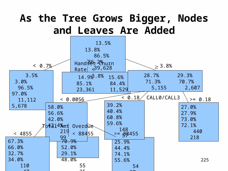
225
25.9% 44.4%74.1% 55.6% 54 27
As the Tree Grows Bigger, Nodesand Leaves Are Added
13.5% 13.8% 86.5% 86.2% 39,628 19,814
3.5% 3.0% 96.5% 97.0% 11,112 5,678
14.9% 15.6% 85.1% 84.4% 23,361 11,529
28.7% 29.3% 71.3% 70.7% 5,155 2,607
< 0.7% Handset Churn Rate< 3.8% 3.8%
58.0% 56.6%42.0% 43.4% 219 99
39.2% 40.4%60.8% 59.6% 148 57
27.0% 27.9%73.0% 72.1% 440 218
CALL0/CALL3< 0.0056 < 0.18 >= 0.18
Total Amt Overdue
67.3% 66.0%32.7% 34.0% 110 47
70.9% 52.0%29.1% 48.0% 55 25
< 4855 < 88455 >= 88455
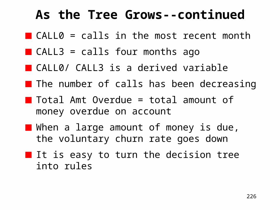
226
As the Tree Grows--continued
CALL0 = calls in the most recent month
CALL3 = calls four months ago
CALL0/ CALL3 is a derived variable
The number of calls has been decreasing
Total Amt Overdue = total amount of money overdue on account
When a large amount of money is due, the voluntary churn rate goes down
It is easy to turn the decision tree into rules
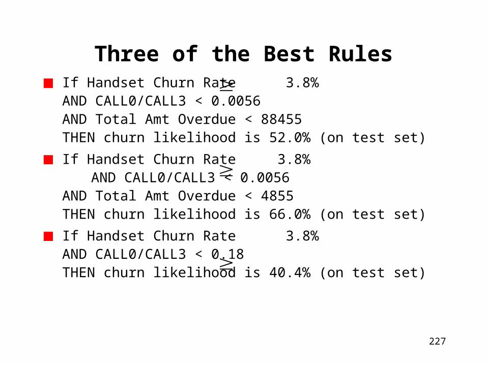
227
Three of the Best RulesIf Handset Churn Rate 3.8%AND CALL0/CALL3 < 0.0056AND Total Amt Overdue < 88455THEN churn likelihood is 52.0% (on test set)
If Handset Churn Rate 3.8% AND CALL0/CALL3 < 0.0056
AND Total Amt Overdue < 4855THEN churn likelihood is 66.0% (on test set)
If Handset Churn Rate 3.8%AND CALL0/CALL3 < 0.18THEN churn likelihood is 40.4% (on test set)
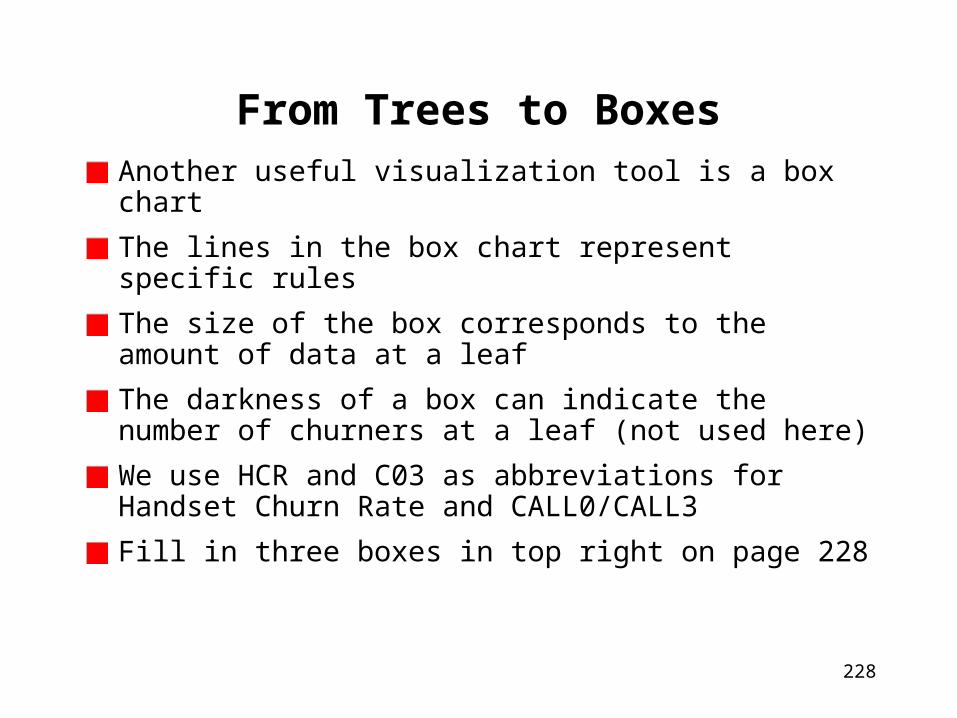
228
From Trees to Boxes
Another useful visualization tool is a box chart
The lines in the box chart represent specific rules
The size of the box corresponds to the amount of data at a leaf
The darkness of a box can indicate the number of churners at a leaf (not used here)
We use HCR and C03 as abbreviations for Handset Churn Rate and CALL0/CALL3
Fill in three boxes in top right on page 228

229
From Trees to Boxes--continued
HCR 3.8%
C03 < 0.18
C03 0.0056
HCR 3.8%
C03 0.18%
HCR < 0.7%0.7% HCR < 3.8%

230
Finding a Good Split at a Decision Tree Node
There are many ways to find a good split
But, they have two things in commonsplits are preferred where the children are similar in sizesplits are preferred where each child is as pure as possible
Most algorithms seek to maximize the purity of each of the children
This can be expressed mathematically, but it is not our focus here

231
Synonymous Splits
There are many ways to determine that the number of calls is decreasing
low amount paid for callssmall number of local callssmall amount paid for international calls
Different variables may be highly correlated or essentially synonymous
Decision trees choose one of a set of synonymous variables to split the data
These variables may become input variables to neural network models

232
Lurking Inside Big Complex Decision Trees Are Simpler, Better Ones

233
Problem: Overfitting the Data
Amt Overdue< 88455
Handset Churn Rate 3.8%
13.5% 13.8% 86.5% 86.2% 39,628 19,814
28.7% 29.3% 71.3% 70.7% 5,155 2,607
58.0% 56.6% 42.0% 43.4% 219 99
70.9% 52.0% 29.1% 48.0% 55 25
CALL0/CALL3< 0.0056
Total
Good! The training set and test set are about the same
Good! The training set and test set are about the same
Good! The training set and test set are about the same
X Ouch! The tree has memorized the
training set, but not generalized
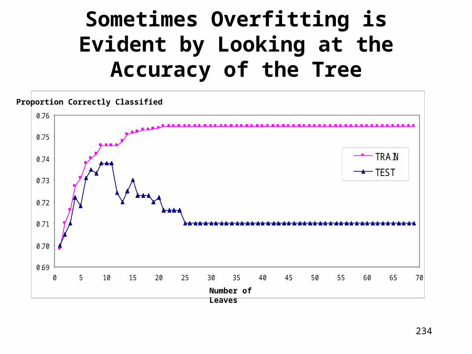
234
Sometimes Overfitting is Evident by Looking at the Accuracy of the Tree
0.69
0.70
0.71
0.72
0.73
0.74
0.75
0.76
0 5 10 15 20 25 30 35 40 45 50 55 60 65 70
TRAIN
TEST
Proportion Correctly Classified
Number of Leaves

235
Prune here This is a good model Error rate is minimized
on unseen data
Pruning the Tree
ErrorRate
Number of Leaves
Test data
Training data
236
Connecting Decision Trees and Lift
A decision tree relating to fraud within the insurance industry is presented next
Assume the analysis is based on test set data
The cumulative gains chart consists of a series of line segments
Each segment corresponds to a leaf of the tree
The slope of each line corresponds to the lift at that leaf
The length of each segment corresponds to the number of records at the leaf
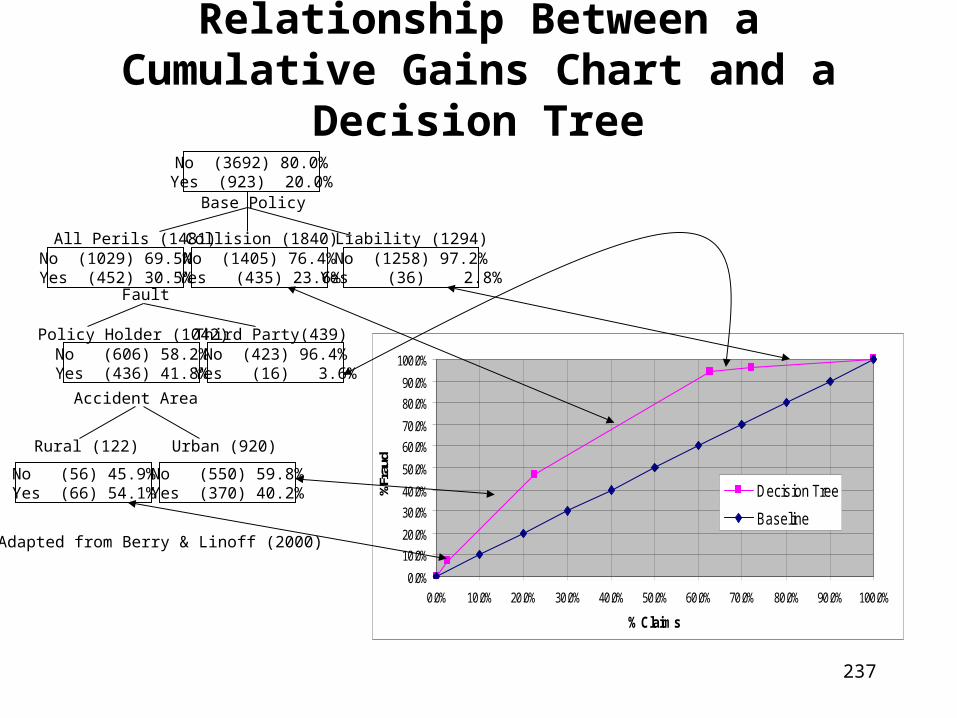
237
Relationship Between a Cumulative Gains Chart and a Decision Tree
No (3692) 80.0%Yes (923) 20.0%
No (1029) 69.5%Yes (452) 30.5%
No (1405) 76.4%Yes (435) 23.6%
No (1258) 97.2%Yes (36) 2.8%
Base Policy
All Perils (1481) Collision (1840) Liability (1294)
Fault
No (606) 58.2%Yes (436) 41.8%
No (423) 96.4%Yes (16) 3.6%
Policy Holder (1042) Third Party(439)
Accident Area
No (56) 45.9%Yes (66) 54.1%
No (550) 59.8%Yes (370) 40.2%
Rural (122) Urban (920)
Adapted from Berry & Linoff (2000)
0.0%
10.0%
20.0%
30.0%
40.0%
50.0%
60.0%
70.0%
80.0%
90.0%
100.0%
0.0% 10.0% 20.0% 30.0% 40.0% 50.0% 60.0% 70.0% 80.0% 90.0% 100.0%
% Claims
%Fr
aud
Decision Tree
Baseline
238
Decision Trees: A Summary
It is easy to understand results
Can be applied to categorical and ordered inputs
Finds inputs (factors) that have the biggest impact on the output
Works best for binary outputs
Powerful software is available
Care must be taken to avoid overfitting
239
Case Study: Churn Prediction
Predicting who is likely to churn at a cellular phone company
The cellular telephone industry is rapidly maturing
The cost of acquiring new customers is rather high
A handset is discounted in exchange for a time commitment
As the market matures, it becomes cheaper to retain than acquire customers
Review the difference between voluntary, forced, and expected attrition
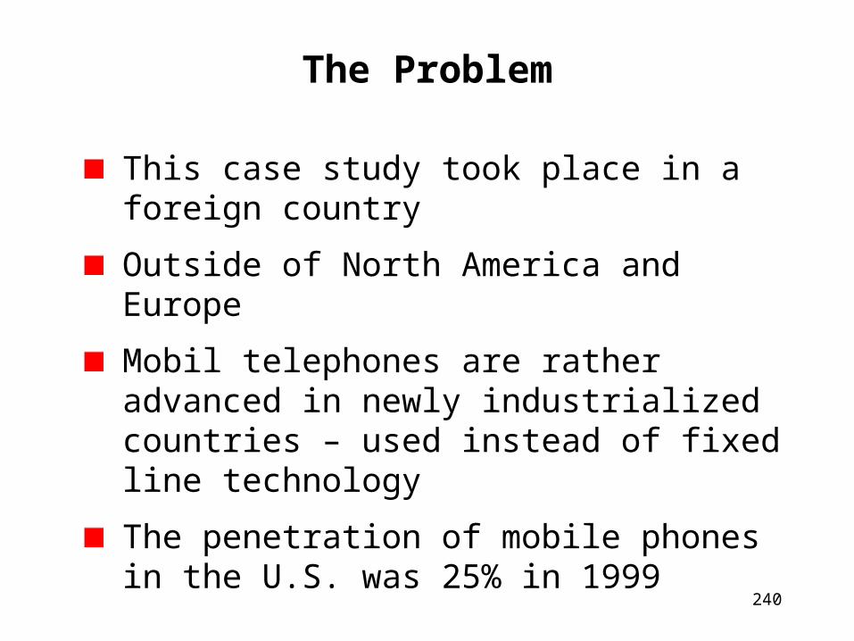
240
The Problem
This case study took place in a foreign country
Outside of North America and Europe
Mobil telephones are rather advanced in newly industrialized countries – used instead of fixed line technology
The penetration of mobile phones in the U.S. was 25% in 1999
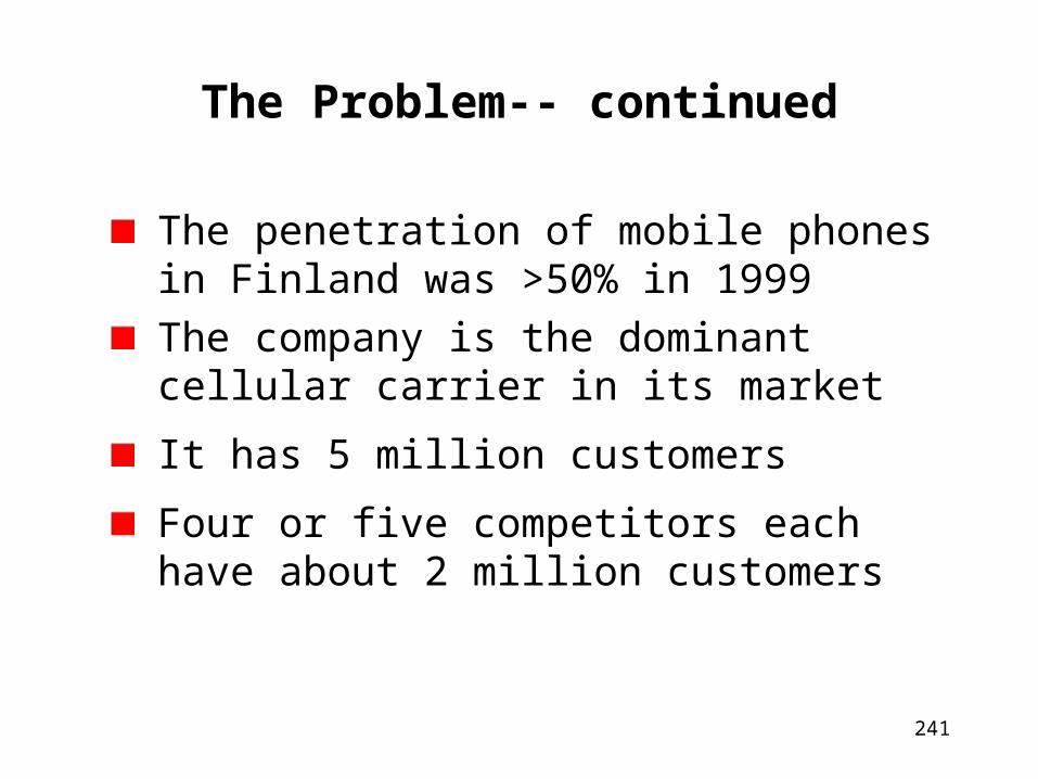
241
The Problem-- continued
The penetration of mobile phones in Finland was >50% in 1999
The company is the dominant cellular carrier in its market
It has 5 million customers
Four or five competitors each have about 2 million customers
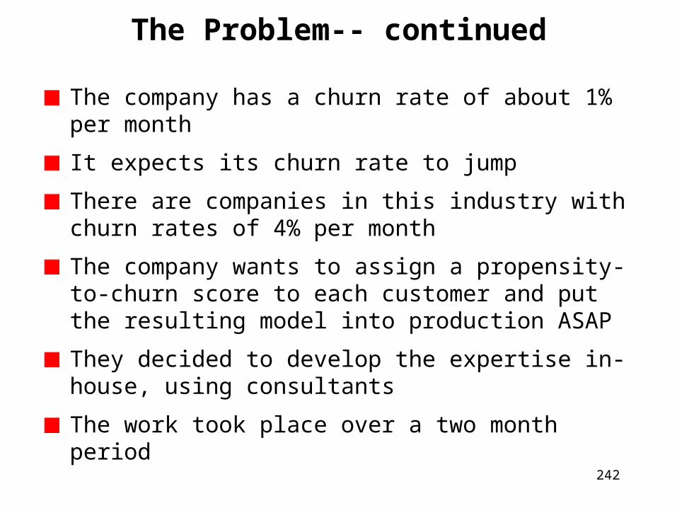
242
The Problem-- continued
The company has a churn rate of about 1% per month
It expects its churn rate to jump
There are companies in this industry with churn rates of 4% per month
The company wants to assign a propensity-to-churn score to each customer and put the resulting model into production ASAP
They decided to develop the expertise in-house, using consultants
The work took place over a two month period
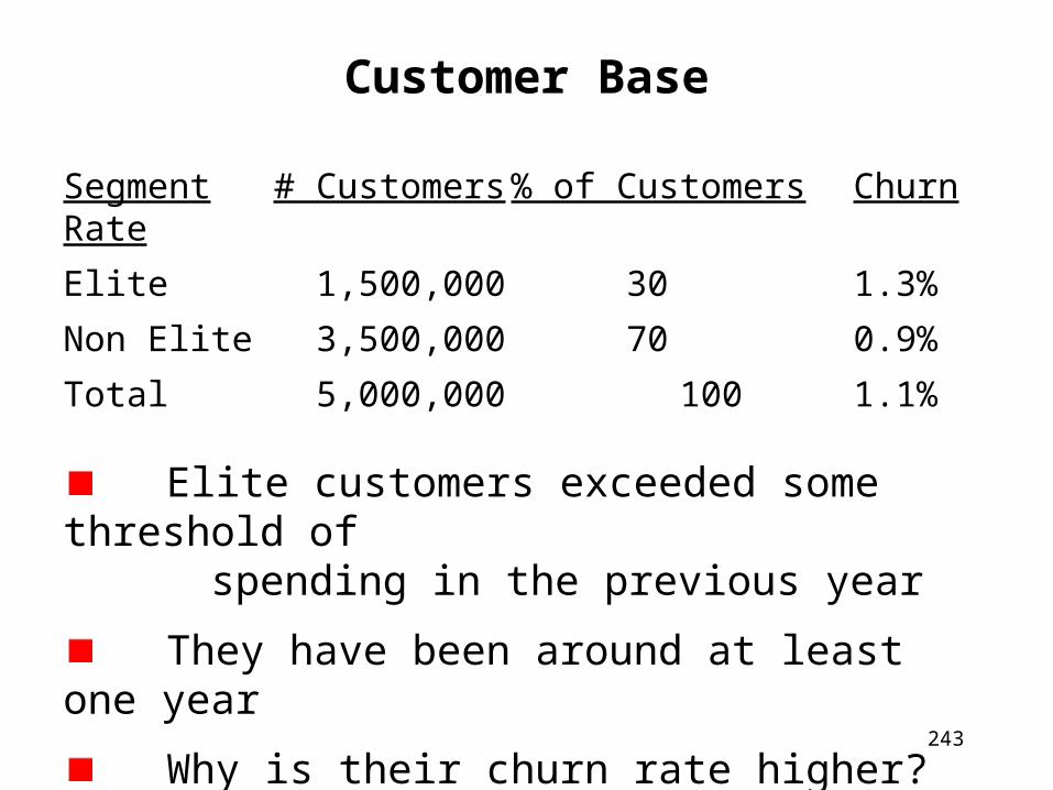
243
Customer Base
Segment # Customers % of Customers Churn Rate
Elite 1,500,000 30 1.3%
Non Elite 3,500,000 70 0.9%
Total 5,000,000 100 1.1%
Elite customers exceeded some threshold of spending in the previous year
They have been around at least one year
Why is their churn rate higher?

244
Data Inputs
Customer information file – telephone number, billing plan, zip code, additional services, Elite Club grade, service activation date, etc.
Handset information – type, manufacturer, weight, etc.
Dealer information – marketing region and size
Billing history
Historical churn rate information by demographics and handset type

245
The Model Set Uses Overlapping Time Windows
Jan Feb Mar Apr May Jun Jul Aug Sep Oct Nov
Model Set 6 5 4 3 2 1 +1
Model Set 6 5 4 3 2 1 +1
Score Set 6 5 4 3 2 1 +1
For the model set, August and September churners are used
We want to use the model to make predictions for November
246
Solving the Right Business Problem
Initial problem: assign a churn score to all customers
Complicating issues new customers have little call history
telephones? individuals? families?
voluntary churn versus involuntary churn
how will the results be used?
Revised problem: by Sept. 20th, provide a list of the 10,000 Elite customers who are most likely to churn in October
The revised problem invites action

247
Build a Number of Churn Models
Numerous decision tree models were built
It was discovered that some customers were taking advantage of the family plan to obtain better handsets at minimal cost
These customers used the marketing campaigns to their own advantage
Different parameters were used to build different models
The density of churners in the model set was one important parameter (50% worked well)

248
Database Marketing and the Catalog Industry
Catalogs are everywhere
For many people, catalogs are the preferred method of shopping
Their resemblance to magazines is intentional
For many people, the reaction is the same
Catalogs are very oldthe first Sears catalog was published in 1888
Catalogs flourished over the next half centuryrailroad, coast-to-coast mail service, mass-produced goods
249
Catalogs are Part of the Retail Business
Catalog retailers know their customersas well as their merchandise
They communicate one-to-oneand not just through branding and mass market advertising
Ability to customize catalogs
Closely related to B2C Web retailing
Many companies (e.g., Eddie Bauer) have stores, catalogs, and a retail Web site
250
The Catalog Industry
$95 billion industry in U.S. (Catalog Age, 1998)
Catalog sales are approximately 10% of all U.S. retail sales
B2C Web retail sales are approximately 1% of U.S. retail sales (1999)
Most catalogs now have an online presence
It is becoming difficult to distinguish between Web retailers and catalog companies

251
What do Catalogers Care About?
Merchandisinghow to display and promote the sale of goods and services?
Layoutwhere to place items in the catalog?which models to use?
Responsecloser to the subject of this coursepersonalization, customization, recommendationwhich of several pre-assembled catalogs should be sent to a specific customer based on an estimate of his response to each?

252
Example of a Big Catalog: Fingerhut
Manny Fingerhut started database marketing in 1948 in Minneapolis
sold seat covers on credit to new car buyers
Fingerhut and specialty catalogs emerged over time
As of the late 1990s$2 billion in annual sales
400 million catalogs/year (> 1 million/day)
terabytes of transaction history
customer and prospect file with 1,400 fields describing 30 million households
253
Different Catalogers Have Different Approaches
Fingerhut aims for a less affluent audience“4 easy payments of $19.95” is a way to hide higher interest rates
the most profitable customers don’t have to be the wealthiest
Victoria’s Secret sees its catalog as part of its brandingevery mailbox should have one
Eddie Bauer has a multi-channel strategycatalog, retail stores, and Web are equal partners
Many are aimed at a very narrow audience
254
The Luxury of Pooled Data
Unlike other industries, the catalog industry promotes the sharing of data through a company called Abacus
U.S. Air doesn’t know about my travels on TWA or Northwest Airlines
But a catalog company (e.g., Eddie Bauer) can decide to send you a catalog because of a purchase you made from a competing catalog (e.g., L.L. Bean)
As a consumer, you may have observed that a purchase from catalog A sometimes triggers the arrival of catalog B
255
Abacus and the World Wide Web
Abacus is the catalog industry infomediary1,100 member companiesmaintains a database of over 2 billion transactionsincludes the vast majority of U.S. catalog purchasessells summarized data to member companiesdetails of individual transactions are not revealedfacilitates industry-wide modeling
DoubleClicka leader in Web advertising, now owns Abacusindicates the convergence of online and off-line retailing

256
Another Source of Data
Household data vendorscompanies that compile data on every U.S. household
Acxiom, First Data, Equifax, Claritas, Experian, R.L. Polk
hundreds of variables (demographic, lifestyle, etc.)
database marketers use this data to assemble mailing lists
Available data
internal data on customers
industry-wide data from Abacus
demographic data from household data vendors
257
What Some Big Catalog Companies areDoing with Data Mining
Neural networks are being used to forecast call center staffing needs
New catalog creation
what should go into it?
which products should be grouped together?
who should receive the catalog?
Campaign optimization
258
Eddie Bauer
Eddie Bauer is an interesting case
They seek tomaintain a unified view of the customer across three channels
give the customer a unified view of Eddie Bauer
They are integrating all channels for CRM400 stores
catalogs
Web sales
259
Vermont Country Store (VCS)
Eddie Bauer and other large companies use CRM extensively
What about smaller companies?
VCS is a successful family-owned business
VCS is a $60 million catalog retailer (late 1990s)
VCS first used CRM to improve the targeting of their catalog to increase the response rate
They used SAS Enterprise Miner to achieve a dramatic return on investment

260
Early Company History
Founded by V. Orton in 1945, after he returned from WWII
As a child, he had helped his father and grandfather run a Vermont country store
His first catalog went out in 1945 or 194636 items
12 pages
mailed to 1000 friends and acquaintances
contained articles and editorials
had the feel of a magazine
261
The Next Generation
Son Lyman Orton took over in the 1970she remains as owner and chairman
the CEO is not a family member
Lyman focused on the catalog side of the business
VCS grew by about 50% per year during the 1980swithout data mining
The catalog industry, as a whole, expanded rapidly during the 1980s
262
The Industry Matures
As the catalog industry prospered, it attracted new entrants
Catalogs began to fill every mailbox
Response rates declined
Growth rates declined
The cost of paper and postage increased rapidly
By 1995, more than one-third of catalog firms were operating in the red
VCS was still profitable, but concerned

263
Vermont Country Store Today
They seek to “sell merchandise that doesn’t come back -- to people who do”
$60 million in annual sales
350 employees
Use Enterprise Miner to build response (predictive) models
VCS sells the notion of a simple and wholesome (old-fashioned) New England lifestyle

264
Business Problem: Find the Right Customers
The VCS vision does not appeal to everyone
Historical data on responders and non-responders is used to predict who will respond to the next catalog
Focus on existing customersupside: we need to select a subset of a pre-determined set of customers
downside: we are unable to identify outstanding new prospects
The goal of response modeling is to find the right customers

265
Possible Objectives or Goals
Increase response rate
Increase revenue
Decrease mailing costs
Increase profit
Increase reactivation rate for dormant customers
Increase order values
Decrease product returns
266
RFM: Common Sense in Retailing
Recency: customers who have recently made a purchase are likely to purchase again
Frequency: customers who make frequent purchases are likely to purchase again
Monetary: customers who have spent a lot of money in the past are likely to spend more money now
Each one of these variables is positively correlated with response to an offer
RFM combines all three variables

267
Where to Begin
Any of the previous goals can be addressed via data mining
The first step is to define the goal precisely
The specific goal determines the target variable
Build the customer signaturesorders placed by customer over time
items purchased by category over time
customer information from internal sources
use customer zip code to add external data
purchase household and neighborhood level data
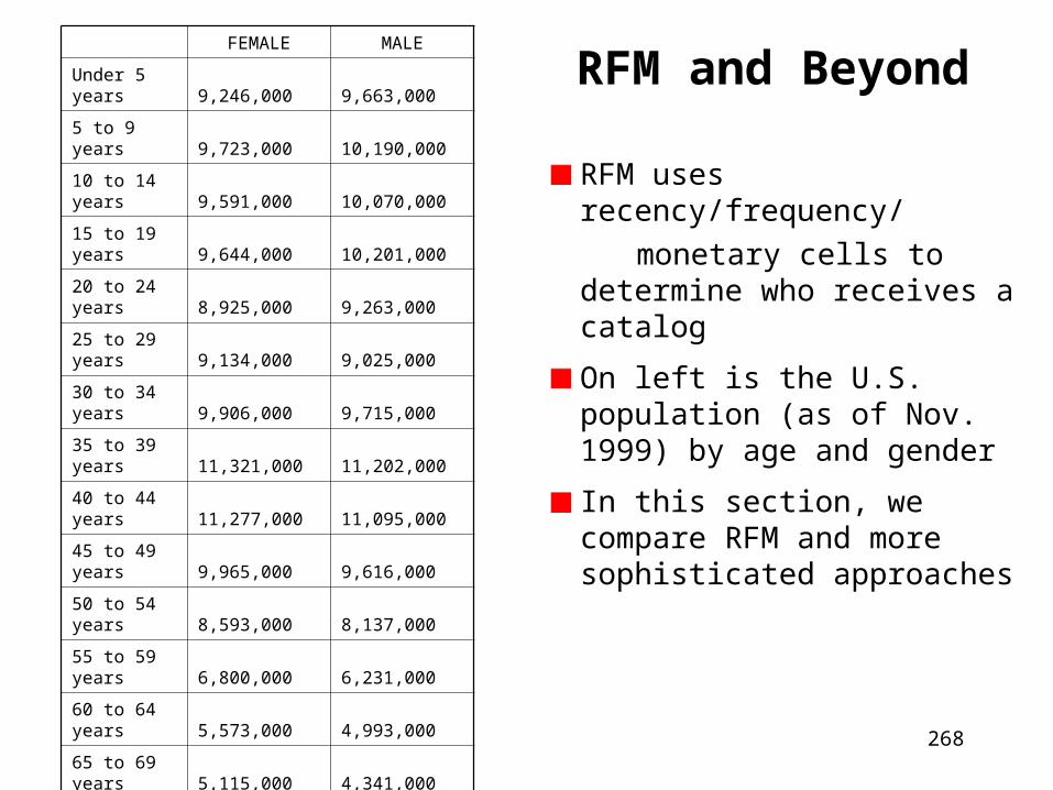
268
RFM and Beyond
RFM uses recency/frequency/
monetary cells to determine who receives a catalog
On left is the U.S. population (as of Nov. 1999) by age and gender
In this section, we compare RFM and more sophisticated approaches
FEMALE MALE
Under 5 years 9,246,000 9,663,000
5 to 9 years 9,723,000 10,190,000
10 to 14 years 9,591,000 10,070,000
15 to 19 years 9,644,000 10,201,000
20 to 24 years 8,925,000 9,263,000
25 to 29 years 9,134,000 9,025,000
30 to 34 years 9,906,000 9,715,000
35 to 39 years 11,321,000 11,202,000
40 to 44 years 11,277,000 11,095,000
45 to 49 years 9,965,000 9,616,000
50 to 54 years 8,593,000 8,137,000
55 to 59 years 6,800,000 6,231,000
60 to 64 years 5,573,000 4,993,000
65 to 69 years 5,115,000 4,341,000
70 to 74 years 4,900,000 3,872,000
75 to 79 years 4,300,000 3,085,000
80 to 84 years 3,021,000 1,836,000
85 to 89 years 1,800,000 864,000
90 to 94 years 851,000 313,000
95 to 99 years 276,000 79,000
100 years & over
51,000 11,000

269
The Cells of the Table Below are Interesting
More boys than girls until age 25
More females than males after age 25
75 – 79 year old men fought in WWII
FEMALE MALE
Under 5 years 48.90% 51.10%
5 to 9 years 48.83% 51.17%
10 to 14 years 48.78% 51.22%
15 to 19 years 48.60% 51.40%
20 to 24 years 49.07% 50.93%
25 to 29 years 50.30% 49.70%
30 to 34 years 50.49% 49.51%
35 to 39 years 50.26% 49.74%
40 to 44 years 50.41% 49.59%
45 to 49 years 50.89% 49.11%
50 to 54 years 51.36% 48.64%
55 to 59 years 51.98% 48.02%
60 to 64 years 52.74% 47.26%
65 to 69 years 54.09% 45.91%
70 to 74 years 55.86% 44.14%
75 to 79 years 58.23% 41.77%
80 to 84 years 62.20% 37.80%
85 to 89 years 67.57% 32.43%
90 to 94 years 73.11% 26.89%
95 to 99 years 77.75% 22.25%
100 years & over 82.26% 17.74%

270
Cell-Based Approaches are Very Popular
RFM is used often in the catalog industry
Cell-based approaches are used to assess credit risk in the banking industry (e.g., CapitalOne)
The insurance industry uses cell-based approaches to assess risk
Market research also uses cell-based approaches, especially when the cells reflect demographics that can be used to predict purchasing behaviors
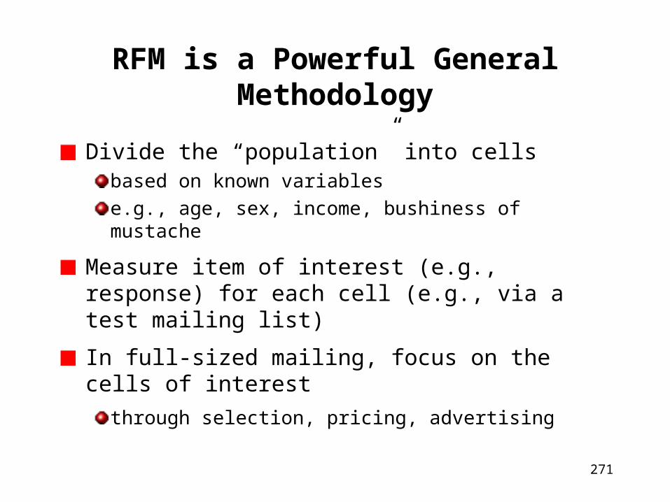
271
RFM is a Powerful General Methodology
Divide the “population” into cellsbased on known variables
e.g., age, sex, income, bushiness of mustache
Measure item of interest (e.g., response) for each cell (e.g., via a test mailing list)
In full-sized mailing, focus on the cells of interest
through selection, pricing, advertising
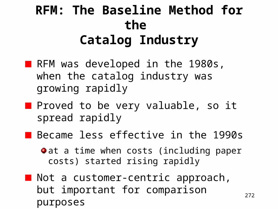
272
RFM: The Baseline Method for the Catalog Industry
RFM was developed in the 1980s, when the catalog industry was growing rapidly
Proved to be very valuable, so it spread rapidly
Became less effective in the 1990s
at a time when costs (including paper costs) started rising rapidly
Not a customer-centric approach, but important for comparison purposes

273
Sort List by Recency
Sort customers from most recent purchase date to least recent
arrangement is based entirely on rank
Break the list into equal-sized sections called quantilestop, bottom
high, medium, low
quartiles
quintiles
deciles
This quantile becomes the R component of the RFM cell assignment
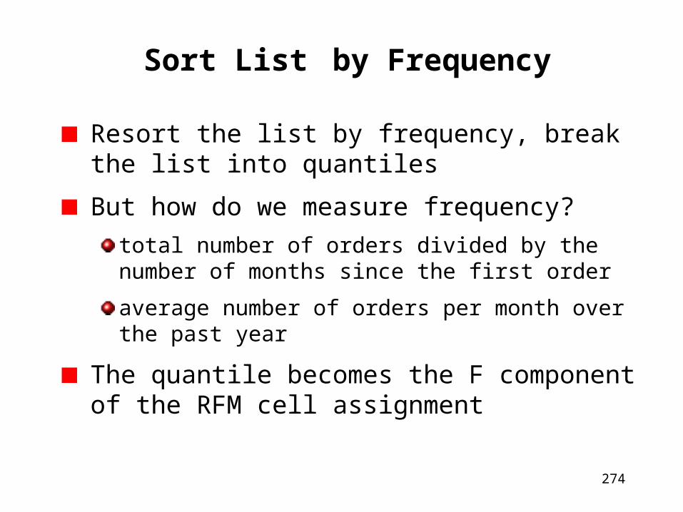
274
Sort List by Frequency
Resort the list by frequency, break the list into quantiles
But how do we measure frequency?
total number of orders divided by the number of months since the first order
average number of orders per month over the past year
The quantile becomes the F component of the RFM cell assignment

275
Sort List by Monetary Value
Resort the list by monetary value, break the list into quantiles
But, what is the right measure?total lifetime spendingaverage dollars per order
The quantile becomes the M component of the RFM cell assignment
Now, imagine a customer whohas not placed an order in a little whiledoesn’t purchase that oftenwhen she does place an order, it tends to be big
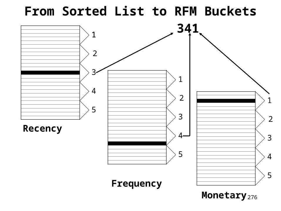
276
From Sorted List to RFM Buckets341
Recency
FrequencyMonetary
1
2
3
4
5
1
1
2
3
4
5
1
2
3
4
5
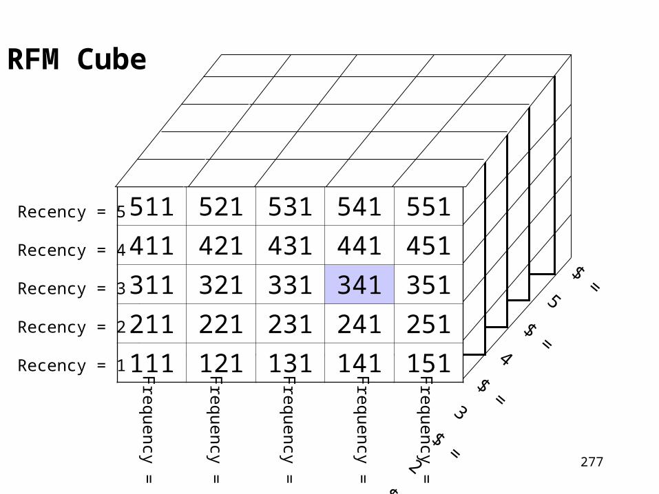
277
RFM Cube
511 521 531 541 551
411 421 431 441 451
311 321 331 341 351
211 221 231 241 251
111 121 131 141 151
Recency = 5
Recency = 4
Recency = 3
Recency = 2
Recency = 1
$ = 5$ = 4$ = 3$ = 2$ = 1
Frequency = 5
Frequency = 4
Frequency = 3
Frequency = 2
Frequency = 1

278
RFM Cells are Not All the Same Size
211 221
111 121
212 222
112 122
15.0% 10.0%
10.0% 15.0%
5.0% 20.0%
20.0% 5.0%
Consider the small example on left
Do the numbers make sense?
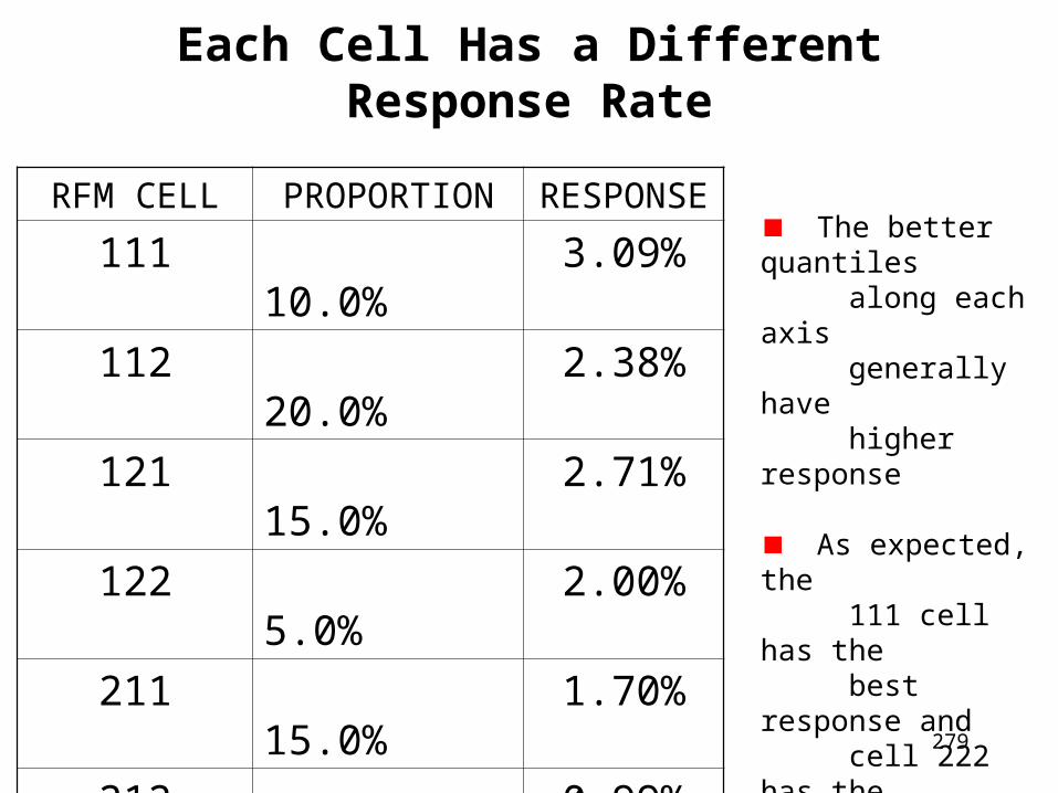
279
Each Cell Has a Different Response Rate
The better quantiles along each axis generally have higher response
As expected, the 111 cell has the best response and cell 222 has the worst
RFM CELL PROPORTION RESPONSE
111 10.0% 3.09%
112 20.0% 2.38%
121 15.0% 2.71%
122 5.0% 2.00%
211 15.0% 1.70%
212 5.0% 0.99%
221 10.0% 1.33%
222 20.0% 0.62%

280
Using RFM Cells to Determine Which Customers Should Receive a Catalog
Given a customer list of one million
Build a cube of 5 x 5 x 5 = 125 RFM cells
Test mail to a random sample with all cells represented
Given a budget that will cover test mail plus sending out 100,000 catalogs
Mail catalogs to customers in top cells with respect to expected response to reach 100,000

281
RFM is a Testing Methodology
RFM involves testing the marketing environment in order to find the best cells
direct test
historical data
Such testing makes good marketing sense
However, it does not use a test set concept, the way we do in building a predictive model
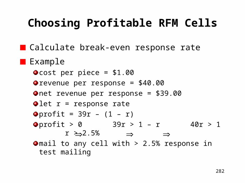
282
Choosing Profitable RFM Cells
Calculate break-even response rate
Examplecost per piece = $1.00
revenue per response = $40.00
net revenue per response = $39.00
let r = response rate
profit = 39r – (1 – r)
profit > 0 39r > 1 – r 40r > 1 r > 2.5%
mail to any cell with > 2.5% response in test mailing
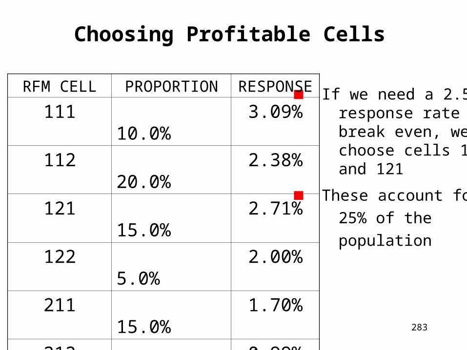
283
Choosing Profitable Cells
If we need a 2.5% response rate to break even, we choose cells 111 and 121
These account for
25% of the
population
RFM CELL PROPORTION RESPONSE
111 10.0% 3.09%
112 20.0% 2.38%
121 15.0% 2.71%
122 5.0% 2.00%
211 15.0% 1.70%
212 5.0% 0.99%
221 10.0% 1.33%
222 20.0% 0.62%
284
Using RFM Cells as Control Groups
VCS wanted to test a new catalog designed to appeal to 53-71 year olds
The motivation was to exploit nostalgia for teenage and young adult years
The new catalog included
color images of products
black and white images of 1950s and 1960s
The test mailing compares target segment against others from the same RFM cell
285
Using Neural Networks for Response Modeling
RFM is our baseline method
RFM has a number of drawbacks
At this time, we seek to gain a basic understanding of neural network models
What are the pitfalls to be avoided?
In this section, we discuss the neural network response model built by VCS

286
Problems with the RFM Approach
RFM cell assignments are not scoresis cell 155 better than cell 311?
a test mailing is required
RFM approach misses important segmentsChristmas shoppers: in November they may look like they have stopped buying from catalog
there may be pockets of good responders in “bad” RFM cells
there may be pockets of bad responders in “good” RFM cells
287
Problems with the RFM Approach -- continued
Proliferation of cellsthere can be a large number of RFM cells
RFM approach hits the same customers over and over
the same people end up in the “best” RFM cellsthese customers suffer from “offer fatigue”
RFM approach does not make use of some valuable data
VCS knows where customers live (demographics)VCS knows about past behavior (purchases, returns, categories)VCS knows which customers are gift givers
288
Problems with RFM Approach -- continued
Focus on cells rather than individualscell-based marketing treats everyone who falls into the same basket the same way
because cell definitions tend to be simplistic, this doesn’t always make sense
Predictive models are more powerful than profilescell definitions are profiles
profiling assigns a customer to a cell whose aggregate behavior is measured
predictive models use input variables to predict future behavior of each customer

289
Back to VCS
After some initial success with RFM in the 1980s, VCS became less enchanted with the technique
In 1998, they were ready to try something new
VCS worked with SAS consultants to see if Enterprise Miner could achieve better results
They compared RFM, regression, neural networks, and decision trees
290
Experimental Design
The model set data came from previous catalog mailings with data on responders and non-responders
Using this data, VCS built RFM, regression, neural network, and decision tree models to predict who would respond to two other mailings that were also in the past, but more recent than the model set data
October mailing
November mailing
Calculate expected response, revenues, and profit assuming models had been used
291
Available Data on Each Customer
Household ID
Number of quarters with at least one order placed
Flags indicating payment by personal check, credit card, or both
Number of catalogs purchased
Number of days since last order
Number of purchases from the various catalog types
Dollars spent per quarter going back several years
Note that R, F, & M are each represented

292
How Models were Judged
Compare regression, neural networks, and decision trees with RFM baseline with respect to percent increase in dollar sales
Look at return on investment in data mining project
How do we guess sales since the comparison is hypothetical?
SAS and VCS were very clever

293
Using Historic Response Data to Compare the Models
Challenger models will pick a different mailing list than the one generated using the RFM approach
How do we guess what someone would have spent had we sent her a catalog, given that we didn’t?
Each model was used to score the list and choose its own top 1.4 million prospects
for actual recipients, use actual dollars spent
for non-recipients, use average spending of recipients with the same score
294
The Results
The neural network model was the model selected by VCS
The model predicted an increase in sales ranging from 2.86% to 12.83%
perhaps, depending on the specific catalog
The model yielded a return on investment of 1,182%
More detailed information is confidential
Let’s revisit the topic of neural networks
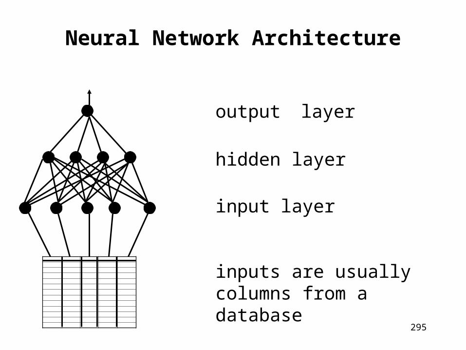
295
Neural Network Architecture
output layer
hidden layer
input layer
inputs are usuallycolumns from adatabase
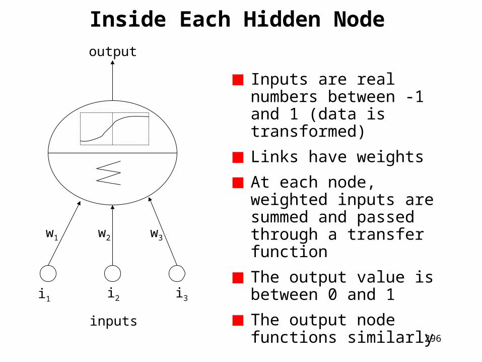
296
Inside Each Hidden Node
Inputs are real numbers between -1 and 1 (data is transformed)
Links have weights
At each node, weighted inputs are summed and passed through a transfer function
The output value is between 0 and 1
The output node functions similarly
i1 i2 i3
w1 w2 w3
inputs
output
297
Training a Neural Network
Given a pre-specified training set and random initial link weights
observe one pattern (a single inputs/output combination) at a time
iteratively adjust the link weights
stop when final weights “best” represent the general relationship between inputs/output combinations
This is called backpropagation
An alternative approach is to use genetic algorithms
298
Procedure for Using Neural Networks
Transform all the input variables to be between -1 and +1 and output variables between 0 and 1
Divide the data into training, testing, and validation sets
Train the neural network using the training set until the error is minimized or the link weights no longer change
Use the test set to choose the best set of weights for the model
Compare models and predict performance using the validation set

299
Neural Networks: Pitfalls to be Avoided
Decision trees can easily handle hundreds of input variablesNeural networks cannot
more input nodes more link weights to be adjusted the larger the training set computationally burdensomeone solution: build a decision tree first and use the variables that appear high in the decision tree in the neural network
Categorical variablese.g., re-renter of Ryder trucks
in the training set, define a variable that takes on the value 1 if the customer is a re-renter and 0 otherwise
300
Neural Networks: Pitfalls to be Avoided-- Continued
Be on the lookout for data skew caused by large outliers
e.g., in looking at net worth, Bill Gates is assigned 1 and everyone else is assigned 0
differences between cardiologists, college professors, and the homeless would be obscured
possible solutions: throw out outliers or perform transformations using logarithms or square roots
301
Final Thoughts on CRM
Cross-sell models: see Chapter 10 in Berry and Linoff (Wiley, 2000)
Data visualization: application to college selection
CRM recap
302
CRM Sources
The vast majority of these CRM slides has been borrowed, adapted, or reworked from one of the two sources below:
1. Michael Berry and Gordon Linoff, Customer Relationship Management Through Data Mining, SAS Institute, 2000
2. Michael Berry and Gordon Linoff, Mastering Data Mining, John Wiley & Sons, 2000
I have also consulted Data Mining Techniques (Wiley, 1997) by Berry and Linoff, in preparing these slides