U. S. FOREST SERVICE RESEARCH PAPER FPL 50 DECEMBER

U. S. DEPARTMENT OF AGRICULTURE FOREST SERVICE FOREST PRODUCTS LABORATORY

OF SIMPLY SUPPORTED PLYWOOD PLATES UNDER COMBINED EDGEWISE BENDING AND COMPRESSION

SUMMARY

Theoretical buckling coefficients for simply sup­ported, flat plywood plates under combined edgewise bending and compression are derived by treating plywood as an orthotropic plate. Curves of buckling coefficients are presented along with two examples of their use. Computational error in the buckling coefficients was held to less than 1 percent.

BUCKLING OF SIMPLY SUPPORTED PLYWOOD PLATES UNDER COMBINED

EDGEWISE BENDING AND COMPRESSION

By JOHN J. ZAHN, Engineer

and KARL M. ROMSTAD, Engineer

FOREST PRODUCTS LABORATORY FOREST SERVICE

U. S. DEPARTMENT OF AGRICULTURE

INTRODUCTION

When a flat plate is subjected to a compressive edge force lying in the plane of the plate. failure can occur by buckling at a stress below the strength of the material. This Research Paper considers the problem of a flat, rectangular plywood plate with all edges simply supported and with edge load in the plane of the plate on two opposite edges. The intensity of this compressive edge force varies linearly along the loaded edges: hence, the resultant of this distribution is a compressive edgewise force P at the center of a loaded edge and an edgewise bending moment M. The relative magnitude of P and M are specified by parameter which varies from 0 <α <2, the extreme values corresponding to pure compression and pure bending, respectively, This problem was solved for a homogeneous plate by Timoshenko2 , but the corresponding solution for an orthotropic plate appears to be lacking in the literature. Accordingly, a mathematical analysis following Timoshenko was undertaken.

The natural orthotropic axes of the plies were taken to be parallel to the coordinate axes. The energy method of solution was used, with the expression for strain energy of bending taken from March’s theory of bending of plywood plates.3 A double sine series was used to represent-the deflected surface of the buckled plate and four terms were retained in the computations, although nearly always three would have been sufficient for less than 1 percent error, Curves were computed with the aid of an IBM 1620 computer and are presented as a family of curves of a nondimensional buckling coefficientversus a reduced aspect ratio. The family is dependent upon two parameters, α and C, the latter con-taining the elastic properties of the plies.

1Maintained at Madison, Wis., in cooperation with the University of Wisconsin.2Timoshenko. S., and Gere, J. Theory of elastic stability. 2nd Ed. McGraw-HiII, 3New York. 1961.

March, H.W. Flat plates of plywood under uniform or concentrated loads. Forest Products Lab. Rpt. 1312. 1942

a, b A

mn C D E1

, E2

E , E x y

E L

, ET

f

F c G

12

G xy h Hni I1, I

2 K K cr , K∞

m, n, i

M N x N , N

o o cr p

P r

U V V o w W e x, y, z α ß

mn λ

NOTATION Length and width of plate (fig. 1). Fourier coefficients of lateral deflection w.

Elastic properties parameter. See equation (15). Mean bending stiffness of plate. See equations (7) and (15). Mean elastic moduli in x and y directions. Associated with bending in equation (7). Also

see equation (27). Elastic moduli of a ply in x and y directions.

Elastic moduli of wood in longitudinal and tangential directions, See discussion following equation (23).

Factor of safety. N xAllowable compressive stress, h , for plywood plate. Depends on species and construction.

shear modulus of plate. Since we took orthotropic axes parallel to edges of plate, we have G

12 = G xy.

Shear modulus of a ply.

Thickness of plate. A function of integers n and i. See equation (15).

Moments of inertia per unit width. See equations (27) and (7),

Load parameter. See equation (15). Buckling coefficients. See equations (20) and (24).

Integers. Edgewise bending moment. See equation (3). Intensity of compressive edge force in x direction, pounds per inch.

Maximum value of NX and its critical magnitude.

Edgewise compressive force. See equation (2). ET = rEL . Ratio dependent on species.

Strain energy of bending. See equation (6). Potential energy of system; strain energy of plate minus work done by loads. Value of V at buckling.

Displacement of middle surface of plate in z direction Work done by loads during buckling.

Coordinates. variation parameter. See equation

see equation (17)

since orthotropic axes are parallel to edges of plate.

Reduced aspect ratio.

Mean Poisson’s ratios of plate. See equation (7).

FPL 50 2

Poisson’s ratios of a ply.

Poisson’s ratios of wood.

MATHEMATICAL ANALYSIS

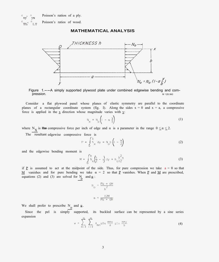
Figure 1.--A simply supported plywood plate under combined edgewise bending and com-pression. M 129 843

Consider a flat plywood panel whose planes of elastic symmetry are parallel to the coordinate planes of a rectangular coordinate system (fig. I). Along the sides x = 0 and x = a, a compressive force is applied in the x direction whose magnitude varies with y:

(1)

where NX is compressive force per inch of edge and α is a parameter in the range 0 < α < 2.

The resultant edgewise compressive force is

(2)

and the edgewise bending moment is

(3)

if P is assumed to act at the midpoint of the side. Thus, for pure compression we take a = 0 so that M vanishes and for pure bending we take α = 2 so that P vanishes. When P and M are prescribed, equations (2) and (3) are solved for N and α : o

We shall prefer to prescribe N and α . o Since the pel is simply supported, its buckled surface can be represented by a sine series

expansion

(4)

3

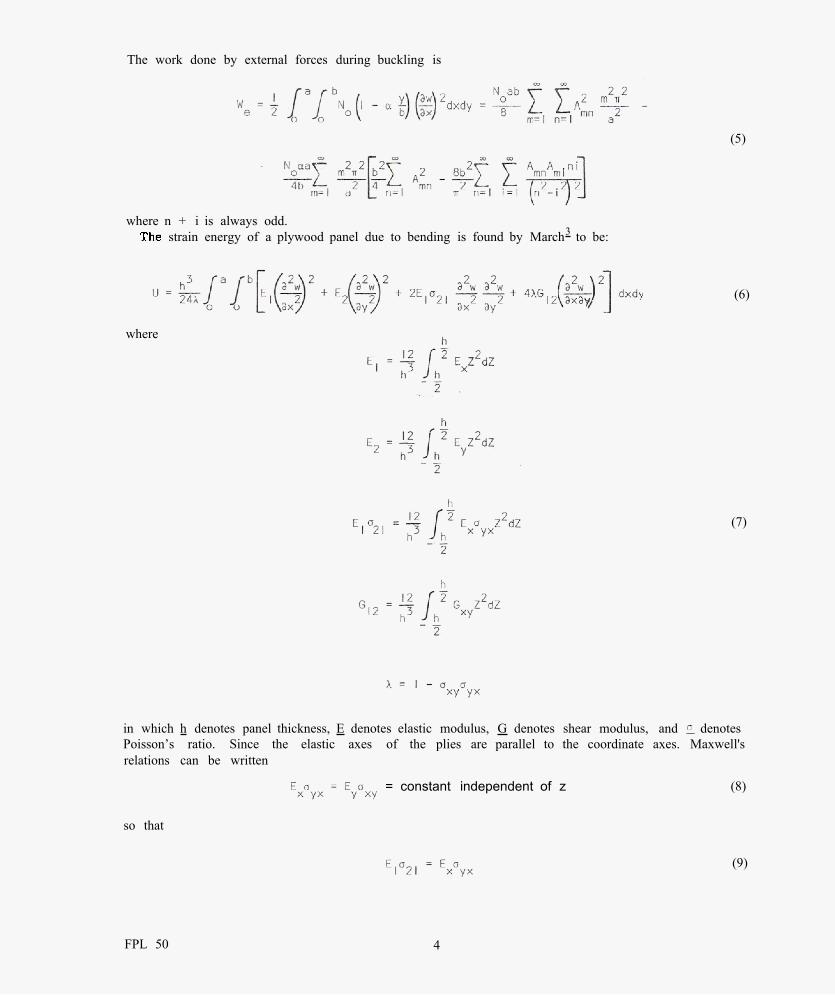
The work done by external forces during buckling is

(5)

where n + i is always odd. strain energy of a plywood panel due to bending is found by March3 to be:

(6)

where

(7)

in which h denotes panel thickness, E denotes elastic modulus, G denotes shear modulus, and denotes Poisson’s ratio. Since the elastic axes of the plies are parallel to the coordinate axes. Maxwell's relations can be written

= constant independent of z (8)

so that

(9)

FPL 50 4

of any ply in this case; also, G 12

= G xy

of any ply and λ is the same in every ply.

Substitituting equation (4) into (6) we obtain

(10)

Now let us write the total energy of the system, taking the unloaded state of Then

(11)

where V is the potential energy of the system just prior to buckling, This term is associated entirelyo with membrane strains of the middle surface of the plate. If the buckling deflections given by (4) are infinitesimal, these membrane strains are constant during buckling; thus, expression (5) is justified and V is seen to be independent of the A . For equilibrium of the system. V is a minimum; hence o mn

(12)

from which

(13)

Using equations (10) and (5), (13) becomes

(14)

The only determinate solution of system (14) is A = 0, all m, n. This corresponds to the flat form mn of equilibrium We now imagine that α is prescribed and N increased until it reaches the value o N at which point the panel buckles and A # 0, for some m. Here the determinant of system (14)o mn cr vanishes. Since there is an infinite set of systems, one for each m, there are infinitely many values of N , one for each The value of m must be chosen by trial to make N a minimum o o

cr cr

5

Before solving for N , we nondimensionalize system (14) by introducing the following notation o cr

(15)

Then, system (14) can be written

(16)

(17)

Then system (16) becomes

(18)

Note that the coefficient array is diagonally symmetric since n and i are interchangeable. and that every other term is zero since every other Hni. is zero. There is an infinity of systems (18), one for

each m. The value of m which yields the least K is dependent upon the reduced aspect ratio, o|. .

NUMERICAL ANALYSIS

System (18) is the condition of equilibrium at buckling if not all A = 0; hence the vanishing of the mn determinant of the coefficients defines a critical value of K which we denote as K . Given o|, C, and cr α, K was chosen by trial to make the determinant vanish, with m chosen so as to minimize K . For

cr small o| , m = An IBM 1620 computer was programmed to start with o| small and m equal to one

FPL 50 6

and to increment o| after each solution for K , thereby generating a plot of K versus o| . Whenever cr cr o| had increased sufficiently, m was increased by unity.

The to increase m was programmed as follows. Let MM denote the current value of m. Figure 2A shows a plot of the value of the determinant versus K for m = MM. The computer plotted this curve and chose K = K by trial so that the determinant was equal to zero, as shown in the cr figure. With this value of K, the computer then calculated one point on the curve for m = MM + 1. If

M 129 844 Figure 2.--Value of determinant versus K, illustrating logic used by when

incrementing o| to decide whether m is yielding the lowest possible value of K cr . In A, computer will increment o| and retain value of m; in B, computer will increment m and decrease value of o| .

the determinant was positive, as figure 2A, the root corresponding to m = MM + 1 was known to be greater than the current K

cr, so was incremented and m = MM was retained. If, however, the

determinant was negative as in figure 2B, the root corresponding to m = MM + 1 was known to be less than the Current K so MM was incremented by unity and o| was not increased. In fact, it was decided cr to decrease o| at this point so that the new branch of the curve of K versus o| for larger m would cr clearly intersect the old branch for smaller m. This provided good definition of the cusps in the

of K versus o|. cr of K versus o| were platted for m = 1, 2, 3, and 4. The envelope of the branches is a cr

horizontal straight line, and since the cusps do not lie much above the envelope for m >4 it was decided to stop computing at m = 4 and show only the straight line envelope for larger o|.

A fourth order determinant was used throughout. Results using a third order determinant were obtained for α = 2 (pure bending), C = 0.2 (the smallest C value and o| >0.4, which showed a difference of 1.02 percent at o| = 0.4 and less than 0.3 percent for larger o|. Hence in

by trial, the increment in K was not refined beyond ∆K = 0.01. The accuracy of the curves is thus more by the scale of the drawings than by computing error.

A flow chart of the computing method and its Fortran coding are given in the Appendix

CURVES OF BUCKLING COEFFICIENTS

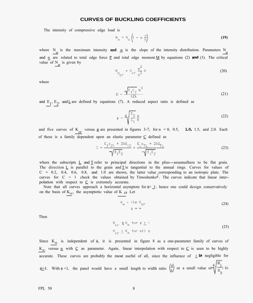
The intensity of compressive edge load is

(19)

where N is the maximum intensity α is the slope of the intensity distribution. Parameters N o o and α are related to total edge force P and total edge moment M by equations (2) (3). The critical value of N is given byo

(20)

where

(21)

and E1, E2, and λ are defined by equations (7). A reduced aspect ratio is defined as

(22)

and five curves of K versus o| are presented in figures 3-7, for α = 0, 0.5, 1.5, and 2.0. Each cr of these is a family dependent upon an elastic parameter C defined as

(23)

where the subscripts L and T refer to principal directions in the plies-assumedhere to be flat grain. The direction L is parallel to the grain and T is tangential to the annual rings. Curves for values of C = 0.2, 0.4, 0.6, 0.8, and 1.0 are shown, the latter value corresponding to an isotropic plate. The curves for C = 1 check the values obtained by Timoshenko2 . The curves indicate that linear inter-polation with respect to C is extremely accurate.

Note that all curves approach a horizontal asymptote for o| > 1; hence one could design conservatively on the basis of K∞, the asymptotic value of K . Let cr

(24)

Then

(25)

Since K∞ is independent of o| , it is presented in figure 8 as a one-parameter family of curves of

K∞ versus α with C as parameter. Again, linear interpolation with respect to C is seen to be highly

accurate. These curves are probably the most useful of all, since the influence of negligible for

o| >1. With o| <1, the panel would have a small length to width ratio or a small value of

FPL 50 8

M 129 846

Figure 3.--Buckling coefficient, K cr, versus reduced aspect ratio, o| , for α=0 (pure com-pression).

either such construction would be uncommon. The curves have two basic uses: (A) select a plywood panel, knowing a, b, P, M, and (B) to

check the stability of a given panel. These will be discussed separately.

A. To Design a Panel

1. Given P, M, and b, find α:

(26)

(27)

9

M 129 847

Figure 4.--Buckling coefficient, K cr, versus- reduced aspect ratio, o| , for α =0.5 (combined

bending and compression).

where I1 = moment of inertia per unit width of parallel plies only; that is, plies whose grain is parallel

to the direction of loading, or x direction. This will ordinarily be the direction of the face grain I2 = moment of inertia per unit width of perpendicular plies only.

Let us introduce a fraction p, which will depend only on the number of plies and their relative thick-nesses, as

(28)

and the ratio

(29)

For most woods 0.01<r<0.07. and r = 0.05 is a good average value. With r introduced, equations (27)

become

(30)

FPL 50 10

M 129 848

Figure 5.--Buckling coefficient, Kcr, versus reduced aspect ratio, o| , for α=1.0 (combined bending and compression).

Assuming that the face grain is parallel to the direction of loading. we can say

Thus rI2 can be neglected in comparison to I1. We cannot neglect rI1 in comparison to I2, however,

since for certain constructions I2 is considerably less than I1. Therefore from equation (30)

11

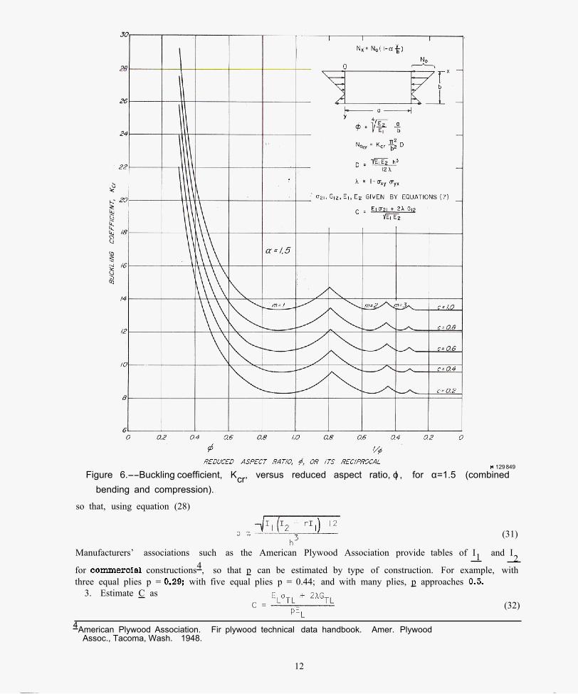
129 849 Figure 6.--Buckling coefficient, Kcr, versus reduced aspect ratio, o| , for α=1.5 (combined

bending and compression).

so that, using equation (28)

(31)

Manufacturers’ associations such as the American Plywood Association provide tables of I1 and I2 for constructions4 , so that p can be estimated by type of construction. For example, with three equal plies p = with five equal plies p = 0.44; and with many plies, p approaches

3. Estimate C as (32)

4American Plywood Association. Fir plywood technical data handbook. Amer. Plywood Assoc., Tacoma, Wash. 1948.

12

M 129 850

Figure 7.--Buckling coefficient, Kcr, versus reduced aspect ratio, o| , for α=2.0 (pure bending).

or, simply make C = 1 on the =et trial. 4. Use α and C to get Kcr from figure 8 for K∞.

5. Get maximum edge load intensity from P, M, and b;

(33)

6. From N and K,o (34)

compute minimum panel thickness using definition of K:

7. Select a panel, recompute p and make a second trial if necessary.

13

M 129 851

Figure 8.--Buckling coefficient, K∞, versus load variation parameter, a, for various values of K∞ is the asymptote of Kcr for large values of o| .

8. Note we have used K∞ for K . Therefore the step is to check If is less than 1 it cr

may be possible to improve the design by using figures 3-7 in lieu of figure 8. 9. This design is based on stability. It should also be checked for strength. Example: Select a 4- by 8-foot Douglas-fir plywood panel to carry an eccentric axial load of

9,000 pounds in the 8-foot direction with an eccentricity of 4 inches and all sides simply supported. Since eccentricity

we have

Anticipating a construction with many equal plies, we estimate

for Douglas-fir. Thus from figure 8, K∞ = 4.0.

Introducing an arbitrary factor of safety of 3, we have P = pounds. Then

FPL 50 14

Thus

h > 0.90 inch; Use h = 0.9375 inch

We select a 15/16-inch, seven ply sanded plywood with 1/8-inch face plies, 3/16-inch centers, and 1/8-inch crossbands for which

Therefore,

which agrees so well with our first estimate that a second trial is unnecessary. A check of ? shows

The allowable compressive stress for this construction (Exterior Grade AB) is 1,375 pounds per

square inch. The maximum compressive stress is pounds per square inch which is less than

the allowable stress.

B. To Check a Given Panel for and Strength

1. Safe loading is determined by

(35)

for stability, where f is a factor of safety,

(36)

for strength, where Fc is the safe allowable compressive stress. Condition (36) can be written

(37)

2. Since Kcr depends on it is convenient to represent conditions (35) and (37) on a plane of

versus α as figure 9. Together, these two conditions define a safe region of the K-α plane. 3. To every point (K, α) in the safe region there a safe pa (P, M) by formulas (2)

and (3). Example: Given a 4-foot by 8-foot by 1-inch Douglas-fir plywood panel for which

15

M 129 845

Figure 9.--Typical shape of safe region of K- α plane. KC is the value of K corresponding to the safe allowable compressive stress.

find the maximum safe load with an eccentricity of 6 inches. Apply a factor of safety 3 to the stability criterion.

As in the earlier example, we know α.

We also compute

FPL 50 16

and obtain K from figure 8 as cr

For safety,

(35)

(37)

In this case stability governs and K = thus max

It must be emphasized that this theory assumes the eccentricity of P is achieved by means of a uniformly varying edge load intensity. For any other boundary condition, the theory must be used with caution.

APPENDIX FLOW CHART OF COMPUTING METHOD

17

FORTRAN PROGRAM FOR BUCKLING OF SIMPLY SUPPORTED PLYWOOD PLATES UNDER COMBINED EDGEWISE

BENDING AND COMPRESSION

FPL 50 18

19

20 1.2-21