bs-nets: an end-to-end framework for band selection of ... › pdf › 1904.08269v1.pdf · bs-nets:...

1

BS-Nets: An End-to-End Framework For BandSelection of Hyperspectral Image

Yaoming Cai, Xiaobo Liu, and Zhihua Cai

Abstract—Hyperspectral image (HSI) consists of hundreds ofcontinuous narrow bands with high spectral correlation, whichwould lead to the so-called Hughes phenomenon and the highcomputational cost in processing. Band selection has been proveneffective in avoiding such problems by removing the redundantbands. However, many of existing band selection methods sepa-rately estimate the significance for every single band and cannotfully consider the nonlinear and global interaction betweenspectral bands. In this paper, by assuming that a complete HSIcan be reconstructed from its few informative bands, we proposea general band selection framework, Band Selection Network(termed as BS-Net). The framework consists of a band attentionmodule (BAM), which aims to explicitly model the nonlinearinter-dependencies between spectral bands, and a reconstructionnetwork (RecNet), which is used to restore the original HSIcube from the learned informative bands, resulting in a flexiblearchitecture. The resulting framework is end-to-end trainable,making it easier to train from scratch and to combine withexisting networks. We implement two BS-Nets respectively usingfully connected networks (BS-Net-FC) and convolutional neuralnetworks (BS-Net-Conv), and compare the results with manyexisting band selection approaches for three real hyperspectralimages, demonstrating that the proposed BS-Nets can accuratelyselect informative band subset with less redundancy and achievesignificantly better classification performance with an acceptabletime cost.

Index Terms—Band selection, Hyperspectral image, Deep neu-ral networks, Attention mechanism, Spectral reconstruction

I. INTRODUCTION

HYPERSPECTRAL images (HSIs) acquired by remotesensors consist of hundreds of narrow bands containing

rich spectral and spatial information, which provides an abilityto accurately recognize the region of interest. Over the pastdecade, HSIs have been widely applied in various fields,ranging from agriculture [1] and land management [2] tomedical imaging [3] and forensics [4].

As the development of hyperspectral imaging techniques,the spectral resolution has been improved greatly, resultingin difficulty of analyzing. According to the characteristic ofhyperspectral imaging, there is a high correlation between

This work was supported in part by the National Natural Science Foun-dation of China under Grant 61773355 and Grant 61603355, in part bythe Fundamental Research Founds for National University, China Universityof Geosciences(Wuhan) under Grant G1323541717, in part by the NationalNature Science Foundation of Hubei Province under Grant 2018CFB528, andin part by the Open Research Project of Hubei Key Laboratory of IntelligentGeo-Information Processing under Grant KLIGIP-2017B01. (Correspondingauthor: X. Liu.)

Y. Cai and Z. Cai are with the School of Computer Science, China Uni-versity of Geosciences, Wuhan 430074, China (e-mail: [email protected];[email protected]).

X. Liu is with the School of Automation, China University of Geosciences,Wuhan 430074, China (e-mail: [email protected]).

adjacent spectral bands [5], [6], [7]. The high-dimensionalHSI data not only increases the time complexity and spacecomplexity but leads to the so-called Hughes phenomenon orcurse of dimensionality [8]. As a result, redundancy reductionbecomes particularly important for HSI processing.

Band Selection (BS) [9], [10], [11], also known as FeatureSelection, is an effective redundancy reduction scheme. Itsbasic idea is to select a significant band subset which includesmost information of the original band set. In contrast to thefeature extraction methods [12] which reduces dimensionalitybased on the complex feature transformation, BS keeps mainphysical property containing in HSIs [5], which makes it easierto explain and apply in practice.

BS methods basically can be classed as supervised andunsupervised methods [13] based on whether the prior knowl-edge is used. Owing to more robust performance and higherapplication prospect, unsupervised BS method has attracted agreat deal of attention over the last few decades. UnsupervisedBS methods can be further divided into three categories:searching-based, clustering-based, and ranking-based methods[14]. The searching-based BS methods treat band selection asa combinational optimization problem and optimize it using aheuristic searching method, such as multi-objective optimiza-tion based band selection (MOBS) [5], [15], [16]. However,heuristic searching methods are generally time-consuming.The clustering-based BS methods assume spectral bands areclusterable [17], [13]. Since the similarity between spectralbands is made full consideration, clustering-based methodshave achieved great success in recent years, for example,subspace clustering (ISSC) [10], [7] and sparse non-negativematrix factorization clustering (SNMF) [18]. The ranking-based BS methods endeavor to assign a rank or weight foreach spectral band by estimating the band significance, e.g.,maximum-variance principal component analysis (MVPCA)[19], sparse representation (SpaBS)[20], [21], and geometry-based band selection (OPBS) [22], etc.

Nevertheless, many existing BS methods are basing onthe linear transformation of spectral bands, resulting in thelack of consideration of the inherent nonlinear relationshipbetween spectral bands. Furthermore, most of the BS methodscommonly view every single spectral band as a separate imageor point and evaluate its significance independently. For ex-ample, clustering-based BS methods are essentially clusteringspectral images with single channel [10], [7], [20]. Therefore,these methods can not take the global spectral interrelationshipinto account and are difficult to combine with various post-processing, such as classification [23].

In this paper, we treat HSI band selection as a spec-

arX

iv:1

904.

0826

9v1

[cs

.CV

] 1

7 A

pr 2

019

http://[email protected]



2

tral reconstruction task assuming that spectral bands can besparsely reconstructed using a few informative bands. Unlikethe existing BS methods, we aim to take full consideration ofthe globally nonlinear spectral-spatial relationship and allowto select significant bands from the complete spectral bandset, even the 3-D HSI cubes. To this end, we design aband selection network (BS-Net) based on using deep neuralnetworks (DNNs) [24], [25] to explicitly model the nonlinearinterdependencies between spectral bands. Although DNNshave been widely used for HSI classification [26], [27],[28] and feature extraction [29], [26], [30], DNN-based bandselection has not attracted much attention yet.

The main contributions of this paper are as follows:1) We proposed an end-to-end band selection framework

based on using deep neural networks to learn the non-linear interdependencies between spectral bands. To thebest of our knowledge, this is among the few deeplearning based band selection methods.

2) We implemented two different BS-Nets according to thedifferent application scenarios, i.e., spectral-based BS-Net-FC and spectral-spatial-based BS-Net-Conv.

3) We extensively evaluated the proposed BS-Nets frame-work from aspects of classification performance andquantitative evaluation, showing that BS-Nets canachieve state-of-the-art results.

The rest of the paper is structured as follows. We firstdefine the notations and review the basic concepts of deeplearning in Section II. Second, we introduce the proposed BS-Net architecture and its implementation in Section III. Next, inSection IV, we explain the experiments that performed to in-vestigate the performance of the proposed methods, comparedwith existing BS methods, and discuss their results. Finally,we conclude with a summary and final remarks in Section V.

II. PRELIMINARY

A. Definition and Notations

We denote a 3-D HSI cube consisting of b spectral bandsand N × M pixels as I ∈ RN×M×b. For convenience, weregard I as a set B = Bibi=1 which contains b band images,where Bi indicates i-th band image. HSI band selection canthus be formally defined as a function ψ : Ω = ψ (B) thattakes all bands as input and produces a band subset with as lessas possible reduction of redundant information and satisfiedΩ ⊆ B, |Ω| = k < b.

In the following, unless as otherwise specified herein, weuniformly use tensors to represent the inputs, outputs, andintermediate outputs involved in the neural networks. Forexample, the input of a convolutional layer is denoted as a4-D tensor x ∈ Rn×m×c, where n ×m is the spatial size ofthe input feature maps, and c is the number of the channels.

B. Convolutional Neural Networks

Deep learning has achieved great success in numerous ap-plications ranging from image recognition to natural languageprocessing [24], [31], [32]. The collection of deep learningmethods includes Convolutional Neural Networks (CNN) [25],

𝐳0 = 𝑥 𝐳1 𝐳2 𝑦

𝑚× 𝑛 × 𝑐 𝑚1 × 𝑛1 × 𝑐1 𝑚2 × 𝑛2 × 𝑐2

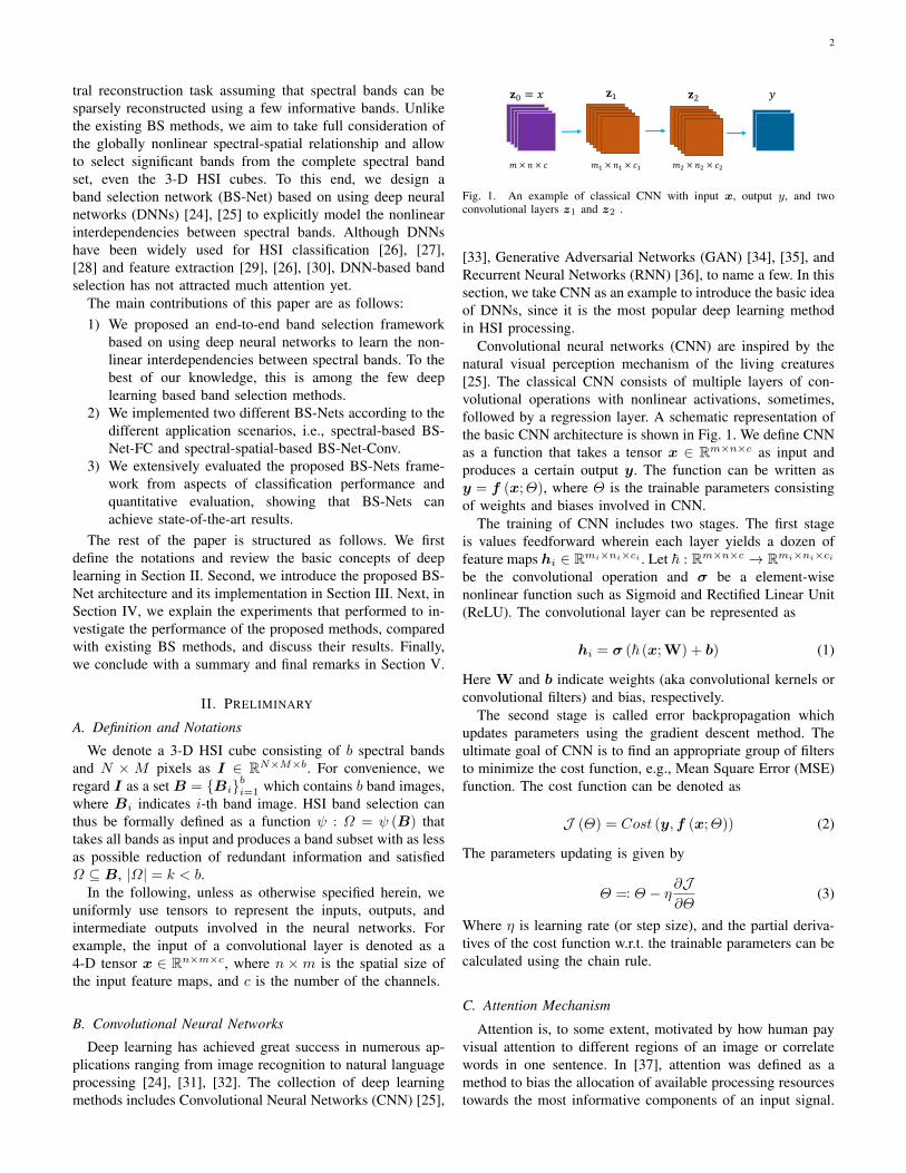
Fig. 1. An example of classical CNN with input x, output y, and twoconvolutional layers z1 and z2 .

[33], Generative Adversarial Networks (GAN) [34], [35], andRecurrent Neural Networks (RNN) [36], to name a few. In thissection, we take CNN as an example to introduce the basic ideaof DNNs, since it is the most popular deep learning methodin HSI processing.

Convolutional neural networks (CNN) are inspired by thenatural visual perception mechanism of the living creatures[25]. The classical CNN consists of multiple layers of con-volutional operations with nonlinear activations, sometimes,followed by a regression layer. A schematic representation ofthe basic CNN architecture is shown in Fig. 1. We define CNNas a function that takes a tensor x ∈ Rm×n×c as input andproduces a certain output y. The function can be written asy = f (x;Θ), where Θ is the trainable parameters consistingof weights and biases involved in CNN.

The training of CNN includes two stages. The first stageis values feedforward wherein each layer yields a dozen offeature maps hi ∈ Rmi×ni×ci . Let ~ : Rm×n×c → Rmi×ni×ci

be the convolutional operation and σ be a element-wisenonlinear function such as Sigmoid and Rectified Linear Unit(ReLU). The convolutional layer can be represented as

hi = σ (~ (x;W) + b) (1)

Here W and b indicate weights (aka convolutional kernels orconvolutional filters) and bias, respectively.

The second stage is called error backpropagation whichupdates parameters using the gradient descent method. Theultimate goal of CNN is to find an appropriate group of filtersto minimize the cost function, e.g., Mean Square Error (MSE)function. The cost function can be denoted as

J (Θ) = Cost (y,f (x;Θ)) (2)

The parameters updating is given by

Θ =: Θ − η ∂J∂Θ

(3)

Where η is learning rate (or step size), and the partial deriva-tives of the cost function w.r.t. the trainable parameters can becalculated using the chain rule.

C. Attention Mechanism

Attention is, to some extent, motivated by how human payvisual attention to different regions of an image or correlatewords in one sentence. In [37], attention was defined as amethod to bias the allocation of available processing resourcestowards the most informative components of an input signal.

3

BAM RecNetHSI

𝑰 ∈ ℝ𝑵×𝑴×𝒃 𝒈(𝒙; 𝜽𝒃) 𝒇(𝒛; 𝜽𝒄)

BRW

⊗

Fig. 2. Overview of Band Selection Networks: A given HSI data isfirst passed onto a Band Attention Module (BAM) to explicitly model thenonlinear interdependencies between spectral bands. Then, the input HSI isre-weighted band-wisely by a Band Re-weighting (BRW) operation. Finally, aReconstruction Network (RecNet) is conducted to restore the original spectralbands from the re-weighted bands.

Mathematically, attention in deep learning can be broadlyinterpreted as a function of importance weights, δ.

ω = δ (x;Θ) (4)

Where ω can be a matrix or vector that indicates the im-portance of a certain input. The implementation of attentionis generally consisting of a gating function (e.g., Sigmoidor Softmax) and combined with multiple layers of nonlinearfeature transformation.

Attention mechanism is widely applied across a range oftasks, including image processing [37], [38], [39] and naturallanguage processing [40], [41], [42]. In this paper, we focusmainly on the attention in visual systems. According to thedifferent concerns of attention methods, visual attention basi-cally can be divided into three categories. The first categoryis spatial attention, which is used to learn the pixel-wiserelationship over the images, such as Spatial TransformerNetworks [38]. Similarly, the second category is focusing onlearning the channel-wise relationship, which is also calledchannel attention, e.g., Squeeze-and-Excitation Networks [37].The third category is the combination of both channel attentionand spatial attention. Thus it is mixed attention, such asConvolutional Block Attention Module [43].

For an HSI band selection task, our goal is to pay moreattention to those informative bands and moreover to avoidthe influence of the trivial bands. Therefore, our proposed BS-Nets are essentially a variant of the channel attention basedmethod and we refer to such an attention used in HSI as BandAttention (BA).

III. BS-NETS

In this section, we first introduce the main componentsincluded in the BS-Nets general architecture. Then, we givetwo versions of implementations of the BS-Nets based onfully connected networks and convolutional neural networks,respectively. Finally, we show a discussion on the BS-Nets.

A. Architecture of BS-Nets

The key to the BS-Nets is to convert the band selection asa sparse band reconstruction task, i.e., recover the completespectral information using a few informative bands. For agiven spectral band, if it is informative then it will be essentialfor a spectral reconstruction. To this end, we design a deep

neural network based on the attention mechanism. In Fig. 2,we show the overall architecture of the proposed framework,which consists of three components: band attention module(BAM), band re-weighting (BRW), and reconstruction network(RecNet). The detailed introduction is given as follows.

The BAM is a branch network which we use to learn theband weights. As shown in Fig. 2, BAM directly takes HSI asinput and aims to fully extract the interdependencies betweenspectral bands. We express BAM as a function g that takes acertain HSI cube x as input and produces a non-negative bandweights tensor, w ∈ R1×1×b.

w = g (x;Θb) (5)

Here Θb denotes the trainable parameters involved in theBAM. To guarantee the non-negativity of the learned weights,Sigmoid function is adopted as the activation of the outputlayer in BAM, which is written as:

φ (w) =1

1 + e−w(6)

To create an interaction between the original inputs and theirweights, a band-wise multiplication operation is conducted.We refer to this operation as BRW. It can be explicitlyrepresented as follows.

z = x⊗w (7)

Where ⊗ indicates the band-wise production between x andw, and z is the re-weighted counterpart of the input x.

In the next step, we employ the RecNet to recover the orig-inal spectral band from the re-weighted counterpart. Similarly,we define the RecNet as a function f that takes a re-weightedtensor z as input and outputs its prediction.

x = f (z;Θc) (8)

Where x is the prediction output for the original input x, andΘc denotes the trainable parameters involved in RecNet.

In order to measure the reconstruction performance, we usethe Mean-Square Error (MSE) as the cost function, denotedas L. We define it as follows:

L =1

2S

S∑i=1

‖xi − xi‖22 (9)

Here S is the number of training samples. Moreover, we desireto keep the band weights as sparse as possible such that wecan interpret them more easily. For this purpose, we imposean L1 norm constraint on the band weights. The resulting lossfunction is given as follows:

L (Θb,Θc) =1

2S

S∑i=1

‖xi − xi‖22 + λ

S∑i=1

‖wi‖1 (10)

Where λ is a regularization coefficient which balances theminimization between the reconstruction error and regular-ization term. Eq. (10) can be optimized by using a gradient

4

BAM Reconstruction NetHSI Pixels

𝒙𝟏

𝒙𝟐

𝒙𝑺

… ⊗BRW

(a) BS-Net-FC.

𝒙𝟏

𝒙𝟐

𝒙𝑺

BAM

⊗

𝑪𝒐𝒏𝒗𝟏

𝑪𝒐𝒏𝒗𝟐

𝑮𝑷𝑭𝑪𝟏 𝑭𝑪𝟐

𝑩𝑹𝑾

𝑪𝒐𝒏𝒗𝟏−𝟏

𝑪𝒐𝒏𝒗𝟏−𝟐

𝑫𝒆𝑪𝒐𝒏𝒗𝟏−𝟐

𝑫𝒆𝑪𝒐𝒏𝒗𝟏−𝟏

𝑪𝒐𝒏𝒗𝟐−𝟏

Conv-DeConv Net 3-D Cubes

…

(b) BS-Net-Conv.

Fig. 3. Implementation details of BS-Nets based on different networks. (a) BS-Net based on fully connected networks with spectral inputs. (b) BS-Net basedon convolutional neural networks with spectral-spatial inputs.

descent method, such as Stochastic Gradient Descent (SGD)and Adaptive Moment Estimation (Adam).

According to the learned sparse band weights, we can de-termine the informative bands by averaging the band weightsfor all the training samples. The average weight of the j-thband is computed as:

wj =1

S

S∑i=1

wij (11)

Those bands which have larger average weights are consideredto be significant since they make more contributions to thereconstruction. In practice, the top k bands are selected as thesignificant band subset. The pseudocode of BS-Nets is givenin Algorithm 1.

Algorithm 1: Pseudocode of BS-Nets

Input: HSI cube: I ∈ RN×M×b; Band subset size: k;and BS-Nets hyper-parameters.

Output: Informative band subset.1 Preprocess HSI and generate training samples;2 Random initialize Θb and Θc according to the given

network configure;3 while Model is convergent or maximum iteration is met

do4 Sample a batch of training samples x;5 Calculate bands weights: w = g (x;Θb);6 Re-weight spectral bands: z = x⊗w;7 Reconstruct spectral bands: x = f (z;Θc);8 Update Θb and Θc by minimizing Eq.(10) using

Adam algorithm;9 end

10 Calculate average band weights according to Eq. (11);11 Select top k bands;

B. BS-Net Based on Fully Connected Networks (BS-Net-FC)

In Fig. 3 (a), we show the first implementation of BS-Netbased on fully modeling the nonlinear relationship between thespectral information. In this case, both of BAM and RecNetare implemented with fully connected networks, and thus werefer to this BS-Net as BS-Net-FC.

As illustrated in Fig. 3 (a), the BAM is designed as abottleneck structure with multiple fully connected layers, with

ReLu activations for all the middle hidden layers. Accordingto the information bottleneck theory [44], bottleneck structurewould be favorable for the extraction of information, althoughdifferent structures are allowed in BS-Nets.

In BS-Net-FC, we use spectral vectors (pixels) as thetraining samples. For convenience, we denote the training setcomprising S samples as a 4-D tensor X ∈ RS×1×1×b, whereS = M × N . By rewriting the band weights in the tensorform, represented as W ∈ RS×1×1×b, the BRW is actuallyan element-wise production operation that can be written asZ = X ⊗W, where Z is the re-weighted spectral inputs. InRecNet, we use a simple multi-layer perceptron model withthe same number of hidden neurons with ReLu activations toreconstruct spectral information.

C. BS-Net Based on Convolutional Networks (BS-Net-Conv)

During the training in BS-Net-FC, only the spectral infor-mation is taken into account. The lack of consideration forthe spatial information would result in low-efficiency use ofthe spectral-spatial information containing in HSI. To enhancethe BS-Net-FC, we implement the second BS-Net by usingconvolutional networks, which is termed as BS-Net-Conv. Theschematic of the implementation is given in Fig. 3 (b).

In the BAM, we first employ several 2-D convolutionallayers to extract spectral and spatial information simultane-ously. Then, a global pooling (GP) layer is used to reducethe spatial size of the resulting feature maps. Finally, the finalband weights W is generated by a few fully connected layerand used to reweight the spectral bands. BS-Net-Conv adopts aconvolutional-deconvolutional network (Conv-DeConv Net) toimplement the RecNet. Similar to the classical auto-encoder,Conv-DeConv Net includes a convolutional encoder whichextracts deep features and a deconvolutional decoder whichup-samples feature maps.

Instead of using single pixels, BS-Net-Conv takes 3-D HSIpatches which includes spectral and spatial information as thetraining samples. To generate enough training samples, weuse a rectangular window of size a × a to slides across thegiven HSI with stride t. The generated training samples canbe denoted as X ∈ RS×a×a×b, where S = M−a

t × N−at + 1.

Notice that the number of training samples in BS-Net-Conv isless than that in BS-Net-FC.

5

D. Remarks on BS-Net framework

The key to our proposed BS-Net framework is to use deepneural networks to explicitly learn spectral bands weights.Compared with the existing band selection methods, the frame-work has the following advantages. The first is the frameworkis end-to-end trainable, making it easy to combine with spe-cific tasks and existed neural networks, such as deep learningbased HSI classification. The second is the framework iscapable of adaptively exacting spectral and spatial information,which avoids hand-designed features and reduces the noiseeffect. The third is the framework is nonlinear, enabling it tomake full exploration of the nonlinear relationship betweenbands. The fourth is the framework is flexible to be imple-mented with diverse networks.

TABLE ISUMMARY OF INDIAN PINES, PAVIA UNIVERSITY, AND SALINAS DATA

SETS.

Data sets Indina Pines Pavia University SalinasPixels 145×145 610×340 512×217

Channels 200 103 204Classes 16 9 16

Labeled pixels 10249 42776 54129Sensor AVIRIS ROSIS AVIRIS

TABLE IIHYPER-PARAMETERS SETTINGS FOR DIFFERENT BS METHODS.

Baselines Hyper-parametersISSC λ = 1e5

SpaBS λ = 1e2MVPCA –SNMF maxiter = 100MOBS maxiter = 100,NP = 100OPBS –

BS-Net-FC λ = 1e− 2,η = 2e− 3,maxiter = 100BS-Net-Conv λ = 1e− 2,η = 2e− 3,maxiter = 100

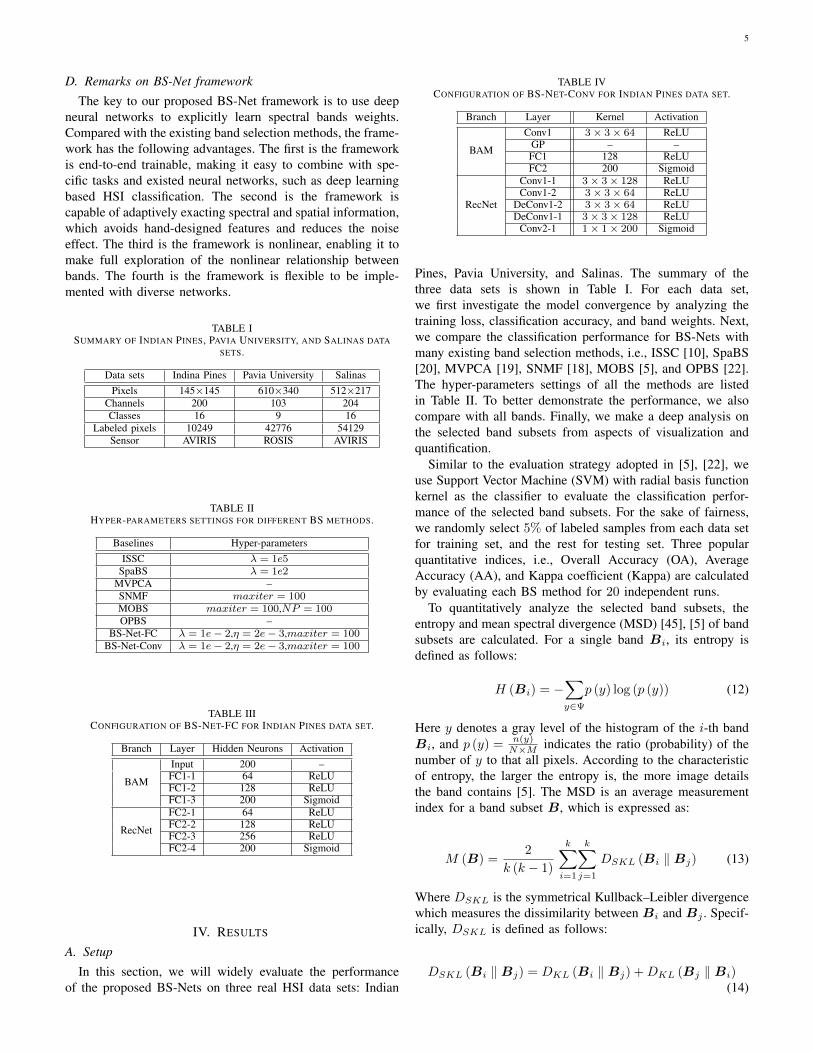
TABLE IIICONFIGURATION OF BS-NET-FC FOR INDIAN PINES DATA SET.

Branch Layer Hidden Neurons Activation

BAM

Input 200 –FC1-1 64 ReLUFC1-2 128 ReLUFC1-3 200 Sigmoid

RecNet

FC2-1 64 ReLUFC2-2 128 ReLUFC2-3 256 ReLUFC2-4 200 Sigmoid

IV. RESULTS

A. Setup

In this section, we will widely evaluate the performanceof the proposed BS-Nets on three real HSI data sets: Indian

TABLE IVCONFIGURATION OF BS-NET-CONV FOR INDIAN PINES DATA SET.

Branch Layer Kernel Activation

BAM

Conv1 3× 3× 64 ReLUGP – –FC1 128 ReLUFC2 200 Sigmoid

RecNet

Conv1-1 3× 3× 128 ReLUConv1-2 3× 3× 64 ReLU

DeConv1-2 3× 3× 64 ReLUDeConv1-1 3× 3× 128 ReLU

Conv2-1 1× 1× 200 Sigmoid

Pines, Pavia University, and Salinas. The summary of thethree data sets is shown in Table I. For each data set,we first investigate the model convergence by analyzing thetraining loss, classification accuracy, and band weights. Next,we compare the classification performance for BS-Nets withmany existing band selection methods, i.e., ISSC [10], SpaBS[20], MVPCA [19], SNMF [18], MOBS [5], and OPBS [22].The hyper-parameters settings of all the methods are listedin Table II. To better demonstrate the performance, we alsocompare with all bands. Finally, we make a deep analysis onthe selected band subsets from aspects of visualization andquantification.

Similar to the evaluation strategy adopted in [5], [22], weuse Support Vector Machine (SVM) with radial basis functionkernel as the classifier to evaluate the classification perfor-mance of the selected band subsets. For the sake of fairness,we randomly select 5% of labeled samples from each data setfor training set, and the rest for testing set. Three popularquantitative indices, i.e., Overall Accuracy (OA), AverageAccuracy (AA), and Kappa coefficient (Kappa) are calculatedby evaluating each BS method for 20 independent runs.

To quantitatively analyze the selected band subsets, theentropy and mean spectral divergence (MSD) [45], [5] of bandsubsets are calculated. For a single band Bi, its entropy isdefined as follows:

H (Bi) = −∑y∈Ψ

p (y) log (p (y)) (12)

Here y denotes a gray level of the histogram of the i-th bandBi, and p (y) = n(y)

N×M indicates the ratio (probability) of thenumber of y to that all pixels. According to the characteristicof entropy, the larger the entropy is, the more image detailsthe band contains [5]. The MSD is an average measurementindex for a band subset B, which is expressed as:

M (B) =2

k (k − 1)

k∑i=1

k∑j=1

DSKL (Bi ‖ Bj) (13)

Where DSKL is the symmetrical Kullback–Leibler divergencewhich measures the dissimilarity between Bi and Bj . Specif-ically, DSKL is defined as follows:

DSKL (Bi ‖ Bj) = DKL (Bi ‖ Bj) +DKL (Bj ‖ Bi)(14)

6

Here DKL (Bi ‖ Bj) can be computed from the gray his-togram information. From Eq. (13), MSD evaluates the redun-dancy among the selected bands, that is, the larger the valueof the MSD is, the less redundancy is contained among theselected bands.

The configuration of BS-Nets implemented in our experi-ments are shown in Table III and Table IV. In reprocessing, wescale all the HSI pixel values to the range [0, 1]. All the base-line methods are evaluated with Python 3.5 running on an IntelXeon E5-2620 2.10 GHz CPU with 32 GB RAM. In addition,we implement BS-Nets with TensorFlow-GPU 1.6 1 and accel-erate them on a NVIDIA TITAN Xp GPU with 11 GB graphicmemory. One may refer to https://github.com/AngryCai for thesource codes and trained models.

B. Results on Indian Pines Data Set

1) Data Set: This scene was gathered by AVIRIS sensorover the Indian Pines test site in North-western Indiana andconsists of 145×145 pixels and 224 spectral reflectance bandsin the wavelength range 0.4–2.5

(×10−6

)meters. The scene

contains two-thirds agriculture, and one-third forest or othernatural perennial vegetation. There are two major dual lanehighways, a rail line, as well as some low-density housing,other built structures, and smaller roads. Since the scene istaken in June some of the crops presents, corn, soybeans, arein early stages of growth with less than 5% coverage. Theground-truth available is designated into sixteen classes and isnot all mutually exclusive. We have also reduced the numberof bands to 200 by removing bands covering the region ofwater absorption: [104− 108], [150− 163], 220.

0 20 40 60 80 100Epoch

45

50

55

60

65

OA (%

)

0

1000

2000

3000

4000

Loss

(a) BS-Net-FC

0 20 40 60 80 100Epoch

52

54

56

58

60

62

64

66

OA (%

)

0

20

40

60

80

100

Loss

(b) BS-Net-Conv

0 25 50 75 100 125 150 175Spectral band

0

20

40

60

80

Epoc

h

0.0

0.2

0.4

0.6

0.8

1.0

(c) BS-Net-FC

0 25 50 75 100 125 150 175Spectral band

0

20

40

60

80

Epoc

h

0.0

0.2

0.4

0.6

0.8

1.0

(d) BS-Net-Conv

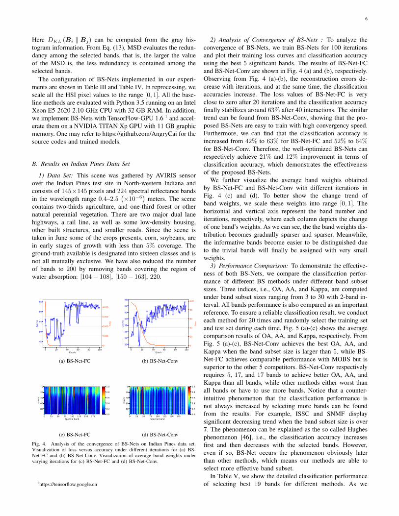
Fig. 4. Analysis of the convergence of BS-Nets on Indian Pines data set.Visualization of loss versus accuracy under different iterations for (a) BS-Net-FC and (b) BS-Net-Conv. Visualization of average band weights undervarying iterations for (c) BS-Net-FC and (d) BS-Net-Conv.

1https://tensorflow.google.cn

2) Analysis of Convergence of BS-Nets : To analyze theconvergence of BS-Nets, we train BS-Nets for 100 iterationsand plot their training loss curves and classification accuracyusing the best 5 significant bands. The results of BS-Net-FCand BS-Net-Conv are shown in Fig. 4 (a) and (b), respectively.Observing from Fig. 4 (a)-(b), the reconstruction errors de-crease with iterations, and at the same time, the classificationaccuracies increase. The loss values of BS-Net-FC is veryclose to zero after 20 iterations and the classification accuracyfinally stabilizes around 63% after 40 interactions. The similartrend can be found from BS-Net-Conv, showing that the pro-posed BS-Nets are easy to train with high convergency speed.Furthermore, we can find that the classification accuracy isincreased from 42% to 63% for BS-Net-FC and 52% to 64%for BS-Net-Conv. Therefore, the well-optimized BS-Nets canrespectively achieve 21% and 12% improvement in terms ofclassification accuracy, which demonstrates the effectivenessof the proposed BS-Nets.

We further visualize the average band weights obtainedby BS-Net-FC and BS-Net-Conv with different iterations inFig. 4 (c) and (d). To better show the change trend ofband weights, we scale these weights into range [0, 1]. Thehorizontal and vertical axis represent the band number anditerations, respectively, where each column depicts the changeof one band’s weights. As we can see, the the band weights dis-tribution becomes gradually sparser and sparser. Meanwhile,the informative bands become easier to be distinguished dueto the trivial bands will finally be assigned with very smallweights.

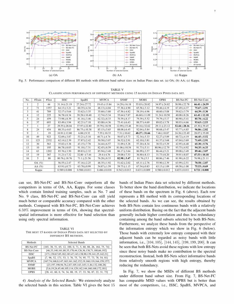
3) Performance Comparison: To demonstrate the effective-ness of both BS-Nets, we compare the classification perfor-mance of different BS methods under different band subsetsizes. Three indices, i.e., OA, AA, and Kappa, are computedunder band subset sizes ranging from 3 to 30 with 2-band in-terval. All bands performance is also compared as an importantreference. To ensure a reliable classification result, we conducteach method for 20 times and randomly select the training setand test set during each time. Fig. 5 (a)-(c) shows the averagecomparison results of OA, AA, and Kappa, respectively. FromFig. 5 (a)-(c), BS-Net-Conv achieves the best OA, AA, andKappa when the band subset size is larger than 5, while BS-Net-FC achieves comparable performance with MOBS but issuperior to the other 5 competitors. BS-Net-Conv respectivelyrequires 5, 17, and 17 bands to achieve better OA, AA, andKappa than all bands, while other methods either worst thanall bands or have to use more bands. Notice that a counter-intuitive phenomenon that the classification performance isnot always increased by selecting more bands can be foundfrom the results. For example, ISSC and SNMF displaysignificant decreasing trend when the band subset size is over7. The phenomenon can be explained as the so-called Hughesphenomenon [46], i.e., the classification accuracy increasesfirst and then decreases with the selected bands. However,even if so, BS-Net occurs the phenomenon obviously laterthan other methods, which means our methods are able toselect more effective band subset.

In Table V, we show the detailed classification performanceof selecting best 19 bands for different methods. As we

https://github.com/AngryCai

7

5 10 15 20 25 30Number of selected bands

10

20

30

40

50

60

70

OA (%

) BS-Net-ConvBS-Net-FCISSCSpaBSMVPCASNMFMOBSOPBSAll bands

(a) OA


10

20

30

40

50

60

70

AA (%


(b) AA


0.1

0.2

0.3

0.4

0.5

0.6

0.7

Kapp

a BS-Net-ConvBS-Net-FCISSCSpaBSMVPCASNMFMOBSOPBSAll bands

(c) Kappa

Fig. 5. Performance comparison of different BS methods with different band subset sizes on Indian Pines data set. (a) OA; (b) AA; (c) Kappa.

TABLE VCLASSIFICATION PERFORMANCE OF DIFFERENT METHODS USING 15 BANDS ON INDIAN PINES DATA SET.

No. #Train #Test ISSC SpaBS MVPCA SNMF MOBS OPBS BS-Net-FC BS-Net-Conv

1 2 44 31.14±21.19 27.24±27.72 19.43±13.84 14.29±16.18 55.03±20.82 34.97±24.82 38.98±22.78 66.41±24.592 71 1357 64.13±3.21 60.35±4.34 48.13±4.04 57.36±4.90 65.56±3.12 59.46±4.19 67.49±4.37 75.67±2.913 41 789 52.17±5.64 53.62±3.35 35.68±3.80 47.56±4.82 58.19±4.96 48.60±5.08 59.62±3.79 64.39±5.304 12 225 36.78±8.34 39.28±10.40 12.74±5.34 35.64±7.87 46.60±11.09 31.24±10.50 40.08±8.26 61.41±12.185 24 459 73.98±8.39 81.16±3.46 62.32±8.33 70.39±8.17 79.39±5.52 79.79±5.17 80.90±5.41 85.78±4.226 37 693 83.49±3.94 82.21±7.18 83.08±4.36 75.41±6.43 88.57±4.69 89.02±3.78 90.93±4.66 93.63±2.537 1 27 29.55±28.04 37.97±22.80 19.79±18.58 12.99±15.46 39.16±32.62 29.11±23.12 52.44±28.16 45.30±39.458 24 454 88.33±4.63 86.75±10.38 85.15±5.65 88.08±6.45 92.04±5.84 90.68±5.47 93.77±4.85 96.86±2.829 1 19 10.91±12.80 6.88±9.32 7.55±10.33 7.31±10.62 48.27±31.66 7.46±10.87 24.26±22.49 28.07±35.09

10 49 923 52.69±3.87 53.21±5.10 40.71±4.74 50.07±5.73 52.34±5.33 52.27±5.09 60.72±4.19 66.45±5.5211 123 2332 62.14±2.39 57.87±2.42 50.58±3.07 56.52±2.91 62.10±3.81 61.37±3.68 67.04±3.69 71.69±2.9112 30 563 35.02±5.38 43.15±7.78 34.44±6.57 31.09±5.28 57.20±8.34 30.52±5.29 42.95±6.48 65.30±5.7613 10 195 86.78±8.03 91.18±7.31 82.45±8.59 81.06±10.54 91.73±5.11 80.96±12.79 93.75±4.92 94.35±6.3314 63 1202 85.76±3.50 89.83±2.32 85.94±3.48 86.17±3.64 86.99±3.57 86.44±5.21 89.08±3.49 89.46±3.0715 19 367 31.21±7.32 32.80 ±7.44 29.4±4.76 29.08±7.53 36.90±8.13 31.73±8.20 39.91±8.07 47.53±10.1816 5 88 80.76±18.76 71.1±21.56 76.28±8.33 82.98±5.47 81.76±5.3 80.86±7.46 81.90±6.22 76.98±21.11

OA (%) 56.55±2.47 57.16±2.25 48.35±1.92 51.62±2.02 65.11±2.76 55.90±2.39 63.99±2.51 70.58±2.87AA (%) 63.91±0.73 63.78±0.99 54.87±1.59 59.75±1.15 67.54±0.83 63.13±1.09 69.58±1.00 75.53±0.69Kappa 0.589±0.008 0.588±0.011 0.486±0.018 0.542±0.013 0.631±0.009 0.580±0.012 0.653±0.011 0.721±0.008

can see, BS-Net-FC and BS-Net-Conv outperform all thecompetitors in terms of OA, AA, Kappa. For some classeswhich contain limited training samples, such as No. 7 andNo. 9 class, BS-Net-FC and BS-Net-Conv can still yieldmuch better or comparable accuracy compared with the othermethods. Compared with BS-Net-FC, BS-Net-Conv achieves6.59% improvement in terms of OA, showing that spectral-spatial information is more effective for band selection thanusing only spectral information.

TABLE VITHE BEST 15 BANDS OF INDIAN PINES DATA SET SELECTED BY

DIFFERENT BS METHODS.

Methods Selected Bands

BS-Net-FC [165, 38, 51, 65, 12, 100, 0, 71, 5, 60, 88, 26, 164, 75, 74]BS-Net-Conv [46,33,140,161,80,35,178,44,126,36,138,71,180,66,192]

ISSC [171,130,67,85,182,183,47,143,138,90,139,141,25,142,21]SpaBS [7, 96, 52, 171, 53, 3, 76, 75, 74, 95, 77, 73, 78, 54, 81]

MVPCA [167,74,168,0,147,165,161,162,152,19,160,119,164,159,157]SNMF [23,197,198,94,76,2,87,105,143,145,11,84,132,108,28]MOBS [5,6,19,24,45,48,105,114,129,142,144,160,168,172,181]OPBS [28, 41, 60, 0, 74, 34, 88, 19, 17, 33, 56, 87, 22, 31, 73]

4) Analysis of the Selected Bands: We extensively analyzethe selected bands in this section. Table VI gives the best 15

bands of Indian Pines data set selected by different methods.To better show the band distribution, we indicate the locationsof these bands on the spectrum in Fig. 6 (above). Each rowrepresents a BS method with its corresponding locations ofthe selected bands. As we can see, the results obtained byboth BS-Nets contain less continuous bands with a relativelyuniform distribution. Basing on the fact that the adjacent bandsgenerally include higher correlation and thus less redundancycontaining among the band subsets selected by both BS-Nets.Furthermore, we analyze these bands from the perspective ofthe information entropy which we show in Fig. 6 (below).Those bands with extremely low entropy compared with theiradjacent bands can be regarded as noisy bands with littleinformation, i.e., [104, 105], [144, 145], [198, 199, 200]. It canbe seen that both BS-Nets avoid these regions with low entropysince these noisy bands make no contribution to the spectralreconstruction. Instead, both BS-Nets select informative bandsfrom relatively smooth regions with high entropy, therebyreducing the redundancy.

In Fig. 7, we show the MSDs of different BS methodsunder different band subset size. From Fig. 7, BS-Net-FChas comparable MSD values with OPBS but is better thanmost of the competitors, i.e., ISSC, SpaBS, MVPCA, and

8

BS-Net-FCBS-Net-Conv

ISSCSpaBSMVPCASNMFMOBSOPBS

0 25 50 75 100 125 150 175 200Spectral band

3.0

3.5

4.0

4.5

5.0

Valu

e of

ent

ropy

Fig. 6. The best 15 bands of Indian Pines data set selected by different BS methods (above) and the entropy value of each band (below).


20

40

60

80

100

MSD

BS-Net-ConvBS-Net-FCISSCSpaBSMVPCASNMFMOBSOPBS

Fig. 7. Mean Spectral Divergence values of different BS methods on IndianPines data set.

MPBS. Although BS-Net-Conv achieves the best classificationperformance, it does not achieve the best MSD. As analyzed in[5], the reason for this phenomenon is that the MSD will alsoincrease if noisy bands are selected, which can be concludedfrom Eq. (13). For instance, the MSDs of band subsets[104, 144] and [104, 25] are 106.64 and 51.49, respectively. Itis obvious that [104, 144] shows much better MSD value than[104, 25], however, [104, 144] contains two completely noisybands which makes less sense to the classification.

C. Results on Pavia University Data Set

1) Data Set: Pavia University data set was acquired by theROSIS sensor during a flight campaign over Pavia, northernItaly. This scene is a 103 spectral bands 610 × 610 pixelsimage, but some of the samples in the image contain noinformation and have to be discarded before the analysis.The geometric resolution is 1.3 meters. The ground-truthdifferentiates 9 classes.

2) Analysis of Convergence of BS-Nets : We show theconvergence curves and the change trend of band weights inFig. 8 (a)-(d). From the results, the loss values tend to be zeroafter several iterations showing that both BS-Nets converge

0 20 40 60 80 100Epoch

78

79

80

81

82

83

OA (%

)

0

20

40

60

80

100

120

Loss

(a) BS-Net-FC

0 20 40 60 80 100Epoch

72

74

76

78

80

82

84

OA (%

)

0.0

0.5

1.0

1.5

2.0

2.5

3.0

Loss

(b) BS-Net-Conv

0 20 40 60 80 100Spectral band

0

20

40

60

80

Epoc

h

0.0

0.2

0.4

0.6

0.8

1.0

(c) BS-Net-FC


0

20

40

60

80

Epoc

h

0.0

0.2

0.4

0.6

0.8

1.0

(d) BS-Net-Conv

Fig. 8. Analysis of the convergence of BS-Nets on Pavia University data set.Visualization of loss versus accuracy under different iterations for (a) BS-Net-FC and (b) BS-Net-Conv. Visualization of normalized average band weightsunder varying iterations for (c) BS-Net-FC and (d) BS-Net-Conv.

well. Meanwhile, as the increase of iteration, the classificationaccuracies of the best five bands are increased from 78%to 83% and 72% to 83% for BS-Net-FC and BS-Net-Conv,respectively.

As shown in Fig. 8 (c)-(d), the average band weights becomevery sparse and easy to distinguish when iteration increases,especially in BS-Net-FC. Finally, only a few significant bands,which are useful to the spectral reconstruction, are highlighted.For example, one can obviously determine that the significantbands of BS-Net-FC are [38, 78, 17, 20, 85] from Fig. 8 (c).Similarly, BS-Net-Conv’s best bands are [90, 42, 16, 48, 71].

3) Performance Comparison: In this experiment, we per-form different BS methods to select different sizes of bandsubsets ranging from 3 to 30. We show the obtained OAs, AAs,and Kappas in Fig. 9 (a)-(c). When band subset size is less than

9


50

60

70

80

90

OA (%


(a) OA


65

70

75

80

85

90

AA (%


(b) AA


0.5

0.6

0.7

0.8

0.9

Kapp


(c) Kappa

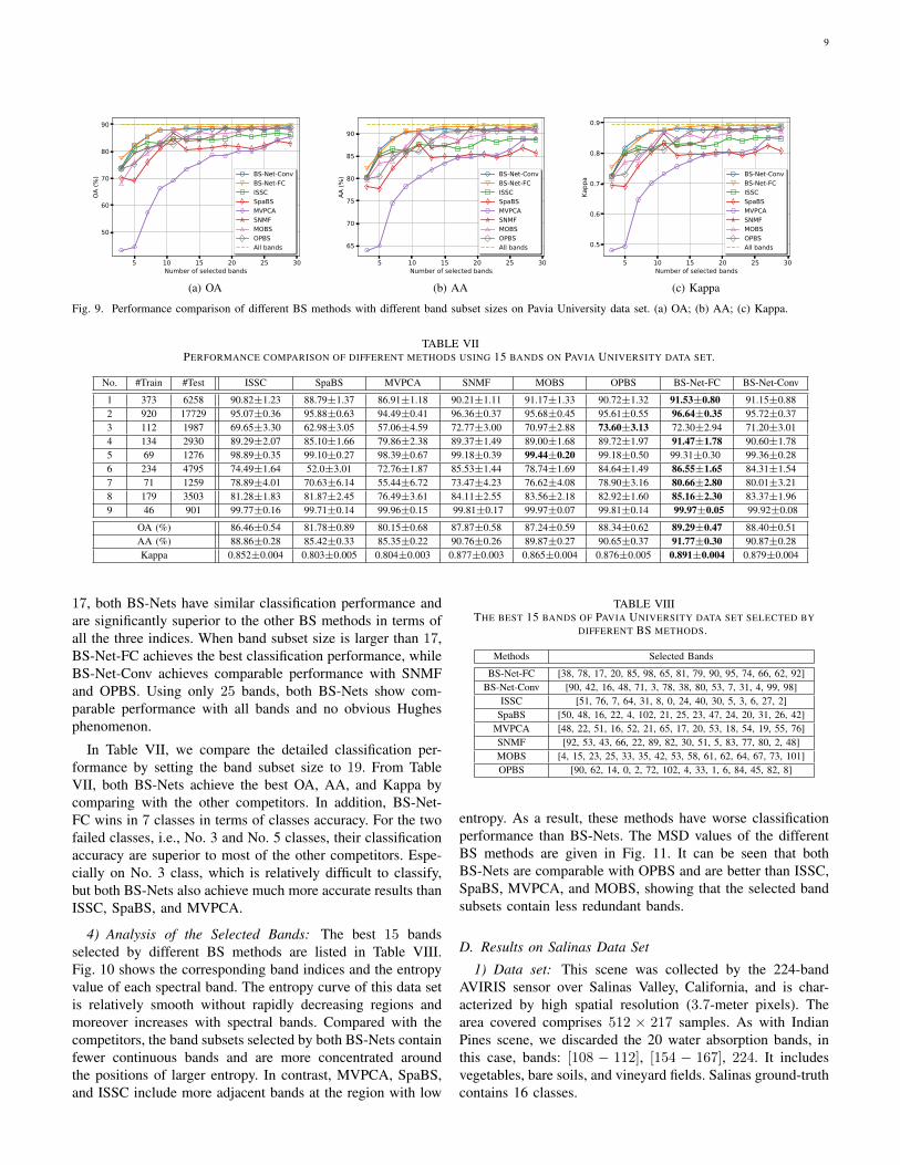
Fig. 9. Performance comparison of different BS methods with different band subset sizes on Pavia University data set. (a) OA; (b) AA; (c) Kappa.

TABLE VIIPERFORMANCE COMPARISON OF DIFFERENT METHODS USING 15 BANDS ON PAVIA UNIVERSITY DATA SET.

No. #Train #Test ISSC SpaBS MVPCA SNMF MOBS OPBS BS-Net-FC BS-Net-Conv

1 373 6258 90.82±1.23 88.79±1.37 86.91±1.18 90.21±1.11 91.17±1.33 90.72±1.32 91.53±0.80 91.15±0.882 920 17729 95.07±0.36 95.88±0.63 94.49±0.41 96.36±0.37 95.68±0.45 95.61±0.55 96.64±0.35 95.72±0.373 112 1987 69.65±3.30 62.98±3.05 57.06±4.59 72.77±3.00 70.97±2.88 73.60±3.13 72.30±2.94 71.20±3.014 134 2930 89.29±2.07 85.10±1.66 79.86±2.38 89.37±1.49 89.00±1.68 89.72±1.97 91.47±1.78 90.60±1.785 69 1276 98.89±0.35 99.10±0.27 98.39±0.67 99.18±0.39 99.44±0.20 99.18±0.50 99.31±0.30 99.36±0.286 234 4795 74.49±1.64 52.0±3.01 72.76±1.87 85.53±1.44 78.74±1.69 84.64±1.49 86.55±1.65 84.31±1.547 71 1259 78.89±4.01 70.63±6.14 55.44±6.72 73.47±4.23 76.62±4.08 78.90±3.16 80.66±2.80 80.01±3.218 179 3503 81.28±1.83 81.87±2.45 76.49±3.61 84.11±2.55 83.56±2.18 82.92±1.60 85.16±2.30 83.37±1.969 46 901 99.77±0.16 99.71±0.14 99.96±0.15 99.81±0.17 99.97±0.07 99.81±0.14 99.97±0.05 99.92±0.08

OA (%) 86.46±0.54 81.78±0.89 80.15±0.68 87.87±0.58 87.24±0.59 88.34±0.62 89.29±0.47 88.40±0.51AA (%) 88.86±0.28 85.42±0.33 85.35±0.22 90.76±0.26 89.87±0.27 90.65±0.37 91.77±0.30 90.87±0.28Kappa 0.852±0.004 0.803±0.005 0.804±0.003 0.877±0.003 0.865±0.004 0.876±0.005 0.891±0.004 0.879±0.004

17, both BS-Nets have similar classification performance andare significantly superior to the other BS methods in terms ofall the three indices. When band subset size is larger than 17,BS-Net-FC achieves the best classification performance, whileBS-Net-Conv achieves comparable performance with SNMFand OPBS. Using only 25 bands, both BS-Nets show com-parable performance with all bands and no obvious Hughesphenomenon.

In Table VII, we compare the detailed classification per-formance by setting the band subset size to 19. From TableVII, both BS-Nets achieve the best OA, AA, and Kappa bycomparing with the other competitors. In addition, BS-Net-FC wins in 7 classes in terms of classes accuracy. For the twofailed classes, i.e., No. 3 and No. 5 classes, their classificationaccuracy are superior to most of the other competitors. Espe-cially on No. 3 class, which is relatively difficult to classify,but both BS-Nets also achieve much more accurate results thanISSC, SpaBS, and MVPCA.

4) Analysis of the Selected Bands: The best 15 bandsselected by different BS methods are listed in Table VIII.Fig. 10 shows the corresponding band indices and the entropyvalue of each spectral band. The entropy curve of this data setis relatively smooth without rapidly decreasing regions andmoreover increases with spectral bands. Compared with thecompetitors, the band subsets selected by both BS-Nets containfewer continuous bands and are more concentrated aroundthe positions of larger entropy. In contrast, MVPCA, SpaBS,and ISSC include more adjacent bands at the region with low

TABLE VIIITHE BEST 15 BANDS OF PAVIA UNIVERSITY DATA SET SELECTED BY



BS-Net-FC [38, 78, 17, 20, 85, 98, 65, 81, 79, 90, 95, 74, 66, 62, 92]BS-Net-Conv [90, 42, 16, 48, 71, 3, 78, 38, 80, 53, 7, 31, 4, 99, 98]

ISSC [51, 76, 7, 64, 31, 8, 0, 24, 40, 30, 5, 3, 6, 27, 2]SpaBS [50, 48, 16, 22, 4, 102, 21, 25, 23, 47, 24, 20, 31, 26, 42]

MVPCA [48, 22, 51, 16, 52, 21, 65, 17, 20, 53, 18, 54, 19, 55, 76]SNMF [92, 53, 43, 66, 22, 89, 82, 30, 51, 5, 83, 77, 80, 2, 48]MOBS [4, 15, 23, 25, 33, 35, 42, 53, 58, 61, 62, 64, 67, 73, 101]OPBS [90, 62, 14, 0, 2, 72, 102, 4, 33, 1, 6, 84, 45, 82, 8]

entropy. As a result, these methods have worse classificationperformance than BS-Nets. The MSD values of the differentBS methods are given in Fig. 11. It can be seen that bothBS-Nets are comparable with OPBS and are better than ISSC,SpaBS, MVPCA, and MOBS, showing that the selected bandsubsets contain less redundant bands.

D. Results on Salinas Data Set

1) Data set: This scene was collected by the 224-bandAVIRIS sensor over Salinas Valley, California, and is char-acterized by high spatial resolution (3.7-meter pixels). Thearea covered comprises 512 × 217 samples. As with IndianPines scene, we discarded the 20 water absorption bands, inthis case, bands: [108 − 112], [154 − 167], 224. It includesvegetables, bare soils, and vineyard fields. Salinas ground-truthcontains 16 classes.

10




4.0

4.2

4.4

4.6

Value of entropy

Fig. 10. The best 15 bands of Pavia University data set selected by different BS methods (above) and the entropy value of each band (below).


1

2

3

4

5

6

7

8

MSD


Fig. 11. Mean Spectral Divergence values of different BS methods on PaviaUniversity data set.

2) Analysis of Convergence of BS-Nets: Fig. 12 (a)-(b)show the convergence curves of BS-Nets on Salinas dataset. Training about 20 iterations, BS-Nets’ loss and accuracyhave tended to be convergent. The OA of using 5 bands areincreased from 92% to 94% and from 85% to 94% for BS-Net-FC and BS-Net-Conv, respectively. In Fig. 12 (c)-(d), we showthe means of band weights under different iterations. Similarto Indian Pines and Pavia University data sets, the learnedband weights become sparse with the increase of iterations.

3) Performance Comparison: The performance comparisonof different BS methods on Salinas data set is shown in Fig.13 (a)-(c). From the results, BS-Net-FC achieves the bestclassification performance when the band subset size is lessthan 19. When band subset size is larger than 19, both BS-Nets are very comparable in terms of OA, AA, and Kappa, andare significantly better than ISSC, SpaBS, MVPCA, SNMF,and OPBS, as well as all bands. Table IX gives the detailedclassification results of using 19 best bands. It can be seen thatboth BS-Nets are generally superior to the other BS methodson most of the classes, and significantly outperform all the

0 20 40 60 80 100Epoch

92.25

92.50

92.75

93.00

93.25

93.50

93.75

94.00

94.25

OA (%

)

0

50

100

150

200

250

300

350

Loss

(a) BS-Net-FC

0 20 40 60 80 100Epoch

90

91

92

93

94

OA (%

)

0

10

20

30

40

50

60

70

80

Loss

(b) BS-Net-Conv

0 25 50 75 100 125 150 175 200Spectral band

0

20

40

60

80

Epoc

h

0.0

0.2

0.4

0.6

0.8

1.0

(c) BS-Net-FC

0 25 50 75 100 125 150 175 200Spectral band

0

20

40

60

80

Epoc

h

0.0

0.2

0.4

0.6

0.8

1.0

(d) BS-Net-Conv

Fig. 12. Analysis of the convergence of BS-Nets on Salinas data set. Lossversus accuracy under different iterations for (a) BS-Net-FC and (b) BS-Net-Conv. Visualization of normalized average band weights under varyingiterations for (c) BS-Net-FC and (d) BS-Net-Conv.

other BS methods in terms of OA, AA, and Kappa.4) Analysis of the Selected Bands: The best 15 bands

selected by different BS methods are shown in Table X. Theirdistribution and entropy are shown in Fig. 14. As we can see,BS-Nets contain less adjacent bands and distribute relativelyuniformly. Observing the entropy curve, both BS-Nets canavoid the sharply decreasing regions with low entropy, i.e.,[106, 107] and [146, 147]. From Fig. 14, some BS methodsinclude a few continuous bands, i.e., OPBS, MVPCA, SpaBS,and ISSC, which means higher correlation is included in theirselected band subsets. Fig. 15 shows the MSD values of differ-ent BS methods, showing that BS-Net-Conv has comparableMSD with ISSC when the band subset size is larger than 15.

11


70

75

80

85

90

95

OA (%


(a) OA


70

75

80

85

90

AA (%


(b) AA


0.65

0.70

0.75

0.80

0.85

0.90

Kapp


(c) Kappa

Fig. 13. Performance comparison of different BS methods with different band subset sizes on Salinas data set. (a) OA; (b) AA; (c) Kappa.

TABLE IXPERFORMANCE COMPARISON OF DIFFERENT METHODS USING 15 BANDS ON SALINAS DATA SET.

NO. #Train #Test ISSC SpaBS MVPCA SNMF MOBS OPBS BS-Net-FC BS-Net-Conv

1 100 1909 99.08±0.49 99.25±0.27 98.99±0.50 99.24±0.46 98.69±0.72 98.76±0.68 99.32±0.55 99.39±0.312 179 3547 99.72±0.34 99.55±0.23 98.47±0.57 99.64±0.22 99.53±0.25 99.69±0.26 99.58±0.37 99.72±0.253 97 1879 98.20±0.74 98.49±0.75 94.20±2.07 96.74±1.48 99.08±0.57 97.20±1.28 99.30±0.37 99.25±0.374 77 1317 99.21±0.62 98.82±0.76 98.97±0.93 98.54±1.08 99.14±0.65 98.76±0.82 98.99±0.61 98.64±1.015 117 2561 98.42±0.58 98.19±0.49 94.78±0.74 96.29±1.19 97.98±0.62 96.96±1.14 97.98±0.80 98.39±0.656 204 3755 99.88±0.06 99.78±0.15 99.38±0.22 99.74±0.13 99.77±0.09 99.79±0.09 99.79±0.11 99.79±0.127 180 3399 99.62±0.23 99.43±0.28 98.90±0.61 99.45±0.29 99.59±0.18 99.56±0.22 99.58±0.23 99.56±0.158 585 10686 82.18±1.76 85.51±1.52 83.51±1.32 85.08±1.50 86.24±1.23 85.06±1.71 87.27±1.60 88.15±1.139 305 5898 99.30±0.38 99.2±0.38 94.14±1.16 99.24±0.39 98.94±0.62 99.06±0.73 99.34±0.38 99.46±0.4210 179 3099 93.57±1.18 90.29±1.01 85.51±2.03 90.97±1.02 93.73±1.25 91.75±1.75 94.95±1.12 94.82±1.0111 47 1021 92.69±2.09 93.73±2.96 65.59±3.93 88.35±4.15 94.21±1.77 95.33±2.91 94.09±3.34 96.19±1.5112 117 1810 98.89±0.92 99.05±0.61 90.51±2.81 97.74±1.03 99.58±0.33 99.47±0.54 99.49±0.88 99.59±0.7113 41 875 98.56±0.80 96.62±2.35 97.78±0.93 96.28±1.96 98.09±1.34 97.57±1.85 98.72±1.25 98.94±0.8514 64 1006 94.24±1.77 95.51±1.28 95.49±1.83 92.78±2.13 95.58±1.08 94.84±1.99 96.18±1.55 96.76±1.5315 337 6931 60.42±3.07 64.81±2.46 56.20±2.6 0 62.53±1.99 69.83±1.92 70.24±2.60 71.60±2.34 70.41±2.2316 77 1730 97.60±0.69 97.55±0.81 96.19±1.36 97.59±0.81 97.76±0.56 98.88±0.21 98.08±0.82 98.65±0.58

OA (%) 94.47±0.21 94.74±0.30 90.54±0.28 93.76±0.37 95.48±0.18 95.18±0.34 95.89±0.31 96.11±0.17AA (%) 89.85±0.18 90.90±0.22 87.10±0.24 90.19±0.22 91.97±0.2 91.60±0.20 92.61±0.19 92.74±0.20Kappa 0.887±0.002 0.899±0.002 0.856±0.003 0.891±0.003 0.911±0.002 0.906±0.002 0.918±0.002 0.919±0.002

TABLE XTHE BEST 15 BANDS OF SALINAS DATA SET SELECTED BY DIFFERENT BS

METHODS.


BS-Net-FC [53, 77, 61, 54, 16, 8, 158, 49, 176, 179, 56, 189, 197, 21, 43]BS-Net-Conv [116,153,19,189,97,179,171,141,95,144,142,46,104,203,91]

ISSC [141,182,106,147,107,146,108,202,203,109,145,148,112,201,110]SpaBS [0, 79, 166, 80, 203, 78, 77, 76, 55, 81, 97, 5, 23, 75, 2]

MVPCA [169,67,168,63,68,78,167,166,165,69,164,163,77,162,70]SNMF [24, 1, 105, 196, 203, 0, 39, 116, 38, 60, 89, 104, 198, 147]MOBS [20,29,35,54,60,62,75,81,93,119,129,132,141,163,201]OPBS [44, 31, 37, 66, 11, 1, 164, 2, 18, 0, 3, 40, 4, 54, 33]

Although SNMF and ISSC achieve the better MSDs, they cannot obtain the best classification performance since few of theirselected bands locate at noisy regions. Similar to the analysisfor Indian Pines data set, these noise bands will increase MSDbut reduce the classification performance. In contrast, BS-Net-FC has relative lower MSD, but it completely avoids noisybands and achieves better classification performance than otherBS methods.

E. Computational Time Complexity Analysis

To analyze the running time, we conduct all the BS methodson the same computer and collect their absolute running time.MOBS and OPBS are implemented in Matlab and the othermethods are implemented in Python. Instead of executing onCPU platform, we train BS-Nets on a GPU platform due toits friendly GPU support. Fig. 16 illustrates the training timeof BS-Net-FC and BS-Net-Conv trained on Indian Pines dataset with different iterations. According to the implementationdetails shown in Table III-IV, BS-Net-FC and BS-Net-Convinclude about 152, 592 and 590, 288 trainable parameters,respectively. However, the number of training samples usedin BS-Net-FC is 21025 while that in BS-Net-Conv is 4489. Itcan be seen from Fig. 16, BS-Net-Conv saves about half ofthe time cost by comparing with BS-Net-FC. It is interestingto notice that the training time is approximatively linear to theiterations.

Table XI shows the computational time of selecting 19bands using different BS methods on the three data sets. It canbe seen that the running times of BS-Nets are comparable withMOBS which bases on heuristic searching and significantlyfaster than SpaBS and SNMF. Since ISSC and MVPCAcan be solved using the algebraic method, they show faster

12



0 25 50 75 100 125 150 175 200Spectral band

1

2

3

4

5

Value of entropy

Fig. 14. The best 15 bands of Salinas data set selected by different BS methods (above) and the entropy value of each band (below).


0

20

40

60

80

100

120

MSD


Fig. 15. Mean Spectral Divergence values of different BS methods on Salinasdata set.

computation speed but cannot achieve better classificationperformance than BS-Nets. In summary, the proposed BS-Netsare able to balance classification performance and runningtime.

0 20 40 60 80 100Epoch

0

100

200

300

400

500

600

700

Trai

ning

tim

e (s

)


Fig. 16. Training time of BS-Nets on Indian Pines data set.

TABLE XICOMPUTATIONAL TIME (IN SECONDS) FOR SELECTING 20 BANDS USING


Method Indian Pines Pavia University SalinasISSC 0.43 14.71 17.44

SpaBS 332.54 2026.80 3224.57MVPCA 0.44 4.24 7.86SNMF > 1h > 1h > 1hMOBS 275.76 289.18 330.30OPBS 2.00 9.62 9.65

BS-Net-FC 652.08 2015.55 1116.99BS-Net-Conv 238.04 493.15 444.37

V. CONCLUSIONS

This paper presents a novel end-to-end band selectionnetwork framework for HSI band selection. The main ideabehind the framework is to treat HSI band selection as a sparsespectral reconstruction task and to explicitly learn the spectralband’s significance using deep neural networks by consideringthe nonlinear correlation between spectral bands. The resultingframework allows to learn band weights from full spectralbands, resulting in more efficient use of the global spectralrelationship, and consists of two flexible sub-networks, bandattention module (BAM) and reconstruction network (RecNet),making it easy to train and apply in practice. The experimentalresults show that the implemented BS-Net-FC and BS-Net-Conv can not only adaptively produce sparse band weights,but also can significantly better classification performance thanmany existing BS methods with an acceptable time cost.

We notice that the proposed framework has the capacityof combining with many deep learning based classificationmethods to reduce computational complexity and enhance theclassification performance. That will also be further exploredin our future works.

13

ACKNOWLEDGMENT

The authors would like to thank the anonymous reviewersfor their constructive suggestions and criticisms. We wouldalso like to thank Dr. W. Zhang who provided the source codesof the OPBS method, and Prof. M. Gong who provided thesource codes of the MOBS method.

REFERENCES

[1] C. M. Gevaert, J. Suomalainen, J. Tang, and L. Kooistra, “Generation ofspectral-temporal response surfaces by combining multispectral satelliteand hyperspectral uav imagery for precision agriculture applications,”IEEE Journal of Selected Topics in Applied Earth Observations andRemote Sensing, vol. 8, no. 6, pp. 3140–3146, June 2015.

[2] J. Pontius, R. P. Hanavan, R. A. Hallett, B. D. Cook, and L. A. Corp,“High spatial resolution spectral unmixing for mapping ash speciesacross a complex urban environment,” Remote Sensing of Environment,vol. 199, pp. 360 – 369, 2017.

[3] B. F. Guolan Lu, “Medical hyperspectral imaging: a review,” Journal ofBiomedical Optics, vol. 19, no. 1, pp. 1 – 24 – 24, 2014.

[4] G. Edelman, E. Gaston, T. van Leeuwen, P. Cullen, and M. Aalders,“Hyperspectral imaging for non-contact analysis of forensic traces,”Forensic Science International, vol. 223, no. 1, pp. 28 – 39, 2012.

[5] M. Gong, M. Zhang, and Y. Yuan, “Unsupervised band selection basedon evolutionary multiobjective optimization for hyperspectral images,”IEEE Transactions on Geoscience and Remote Sensing, vol. 54, no. 1,pp. 544–557, Jan 2016.

[6] W. Sun and Q. Du, “Graph-regularized fast and robust principal compo-nent analysis for hyperspectral band selection,” IEEE Transactions onGeoscience and Remote Sensing, vol. 56, no. 6, pp. 3185–3195, June2018.

[7] H. Zhai, H. Zhang, L. Zhang, and P. Li, “Laplacian-regularized low-rank subspace clustering for hyperspectral image band selection,” IEEETransactions on Geoscience and Remote Sensing, pp. 1–18, 2018.

[8] F. Melgani and L. Bruzzone, “Classification of hyperspectral remotesensing images with support vector machines,” IEEE Transactions onGeoscience and Remote Sensing, vol. 42, no. 8, pp. 1778–1790, Aug2004.

[9] J. Feng, L. Jiao, F. Liu, T. Sun, and X. Zhang, “Mutual-information-based semi-supervised hyperspectral band selection with high discrim-ination, high information, and low redundancy,” IEEE Transactions onGeoscience and Remote Sensing, vol. 53, no. 5, pp. 2956–2969, May2015.

[10] W. Sun, L. Zhang, B. Du, W. Li, and Y. M. Lai, “Band selection usingimproved sparse subspace clustering for hyperspectral imagery classifi-cation,” IEEE Journal of Selected Topics in Applied Earth Observationsand Remote Sensing, vol. 8, no. 6, pp. 2784–2797, June 2015.

[11] Y. Yuan, J. Lin, and Q. Wang, “Dual-clustering-based hyperspectral bandselection by contextual analysis,” IEEE Transactions on Geoscience andRemote Sensing, vol. 54, no. 3, pp. 1431–1445, March 2016.

[12] X. Jiang, X. Song, Y. Zhang, J. Jiang, J. Gao, and Z. Cai, “Laplacianregularized spatial-aware collaborative graph for discriminant analysisof hyperspectral imagery,” Remote Sensing, vol. 11, no. 1, p. 29, 2019.

[13] M. Bevilacqua and Y. Berthoumieu, “Unsupervised hyperspectral bandselection via multi-feature information-maximization clustering,” in2017 IEEE International Conference on Image Processing (ICIP), Sep.2017, pp. 540–544.

[14] W. Sun, L. Tian, Y. Xu, D. Zhang, and Q. Du, “Fast and robust self-representation method for hyperspectral band selection,” IEEE Journalof Selected Topics in Applied Earth Observations and Remote Sensing,vol. 10, no. 11, pp. 5087–5098, Nov 2017.

[15] M. Zhang, M. Gong, and Y. Chan, “Hyperspectral band selectionbased on multi-objective optimization with high information and lowredundancy,” Applied Soft Computing, vol. 70, pp. 604 – 621, 2018.

[16] P. Hu, X. Liu, Y. Cai, and Z. Cai, “Band selection of hyperspectral im-ages using multiobjective optimization-based sparse self-representation,”IEEE Geoscience and Remote Sensing Letters, pp. 1–5, 2018.

[17] Q. Wang, F. Zhang, and X. Li, “Optimal clustering framework forhyperspectral band selection,” IEEE Transactions on Geoscience andRemote Sensing, vol. 56, no. 10, pp. 5910–5922, Oct 2018.

[18] L. I. Ji-Ming and Y. T. Qian, “Clustering-based hyperspectral bandselection using sparse nonnegative matrix factorization,” Frontiers ofInformation Technology and Electronic Engineering, vol. 12, no. 7, pp.542–549, 2011.

[19] C.-I. Chang, Q. Du, T.-L. Sun, and M. L. G. Althouse, “A joint bandprioritization and band-decorrelation approach to band selection forhyperspectral image classification,” IEEE Transactions on Geoscienceand Remote Sensing, vol. 37, no. 6, pp. 2631–2641, Nov 1999.

[20] K. Sun, X. Geng, and L. Ji, “A new sparsity-based band selectionmethod for target detection of hyperspectral image,” IEEE Geoscienceand Remote Sensing Letters, vol. 12, no. 2, pp. 329–333, Feb 2015.

[21] Y. Yuan, G. Zhu, and Q. Wang, “Hyperspectral band selection by mul-titask sparsity pursuit,” IEEE Transactions on Geoscience and RemoteSensing, vol. 53, no. 2, pp. 631–644, Feb 2015.

[22] W. Zhang, X. Li, Y. Dou, and L. Zhao, “A geometry-based bandselection approach for hyperspectral image analysis,” IEEE Transactionson Geoscience and Remote Sensing, vol. 56, no. 8, pp. 4318–4333, Aug2018.

[23] X. Jiang, X. Fang, Z. Chen, J. Gao, J. Jiang, and Z. Cai, “Supervisedgaussian process latent variable model for hyperspectral image classifi-cation,” IEEE Geoscience and Remote Sensing Letters, vol. 14, no. 10,pp. 1760–1764, Oct 2017.

[24] Y. LeCun, Y. Bengio, and G. Hinton, “Deep learning,” Nature, vol. 521,no. 7553, pp. 436–444, 2015.

[25] J. Gu, Z. Wang, J. Kuen, L. Ma, A. Shahroudy, B. Shuai, T. Liu,X. Wang, G. Wang, J. Cai, and T. Chen, “Recent advances in con-volutional neural networks,” Pattern Recognition, vol. 77, pp. 354–377,2018.

[26] Y. Chen, H. Jiang, C. Li, X. Jia, and P. Ghamisi, “Deep feature extractionand classification of hyperspectral images based on convolutional neuralnetworks,” IEEE Transactions on Geoscience and Remote Sensing,vol. 54, no. 10, pp. 6232–6251, 2016.

[27] Q. Liu, F. Zhou, R. Hang, and X. Yuan, “Bidirectional-convolutionallstm based spectral-spatial feature learning for hyperspectral imageclassification,” Remote Sensing, vol. 9, no. 12, p. 1330, 2017.

[28] Z. Zhong, J. Li, Z. Luo, and M. Chapman, “Spectral-spatial residualnetwork for hyperspectral image classification: A 3-d deep learningframework,” IEEE Transactions on Geoscience and Remote Sensing,vol. 56, no. 2, pp. 847–858, 2018.

[29] W. Zhao and S. Du, “Spectral-spatial feature extraction for hyperspectralimage classification: A dimension reduction and deep learning ap-proach,” IEEE Transactions on Geoscience and Remote Sensing, vol. 54,no. 8, pp. 4544–4554, 2016.

[30] L. Jiao, M. Liang, H. Chen, S. Yang, H. Liu, and X. Cao, “Deepfully convolutional network-based spatial distribution prediction forhyperspectral image classification,” IEEE Transactions on Geoscienceand Remote Sensing, vol. 55, no. 10, pp. 5585–5599, 2017.

[31] L. Zhang, L. Zhang, and B. Du, “Deep learning for remote sensingdata: A technical tutorial on the state of the art,” IEEE Geoscience andRemote Sensing Magazine, vol. 4, no. 2, pp. 22–40, 2016.

[32] Y. Cai, X. Liu, Y. Zhang, and Z. Cai, “Hierarchical ensemble of extremelearning machine,” Pattern Recognition Letters, 2018.

[33] D. M. Pelt and J. A. Sethian, “A mixed-scale dense convolutional neuralnetwork for image analysis,” Proc Natl Acad Sci U S A, vol. 115, no. 2,pp. 254–259, 2018.

[34] I. Goodfellow, J. Pouget-Abadie, M. Mirza, B. Xu, D. Warde-Farley,S. Ozair, A. Courville, and Y. Bengio, “Generative adversarial nets,” inAdvances in Neural Information Processing Systems 27, Z. Ghahramani,M. Welling, C. Cortes, N. D. Lawrence, and K. Q. Weinberger, Eds.Curran Associates, Inc., 2014, pp. 2672–2680.

[35] A. Creswell, T. White, V. Dumoulin, K. Arulkumaran, B. Sengupta, andA. A. Bharath, “Generative adversarial networks: An overview,” IEEESignal Processing Magazine, vol. 35, no. 1, pp. 53–65, Jan 2018.

[36] L. Mou, P. Ghamisi, and X. X. Zhu, “Deep recurrent neural networks forhyperspectral image classification,” IEEE Transactions on Geoscienceand Remote Sensing, vol. 55, no. 7, pp. 3639–3655, July 2017.

[37] J. Hu, L. Shen, and G. Sun, “Squeeze-and-excitation networks,” in TheIEEE Conference on Computer Vision and Pattern Recognition (CVPR),June 2018.

[38] M. Jaderberg, K. Simonyan, A. Zisserman, and k. kavukcuoglu, “Spatialtransformer networks,” in Advances in Neural Information ProcessingSystems 28, C. Cortes, N. D. Lawrence, D. D. Lee, M. Sugiyama, andR. Garnett, Eds. Curran Associates, Inc., 2015, pp. 2017–2025.

[39] F. Wang, M. Jiang, C. Qian, S. Yang, C. Li, H. Zhang, X. Wang, andX. Tang, “Residual attention network for image classification,” in TheIEEE Conference on Computer Vision and Pattern Recognition (CVPR),July 2017.

[40] K. Xu, J. Ba, R. Kiros, K. Cho, A. Courville, R. Salakhudinov, R. Zemel,and Y. Bengio, “Show, attend and tell: Neural image caption generationwith visual attention,” in International conference on machine learning,2015, pp. 2048–2057.

14

[41] T. Luong, H. Pham, and C. D. Manning, “Effective approaches toattention-based neural machine translation,” in Proceedings of the 2015Conference on Empirical Methods in Natural Language Processing,2015, pp. 1412–1421.

[42] A. Vaswani, N. Shazeer, N. Parmar, J. Uszkoreit, L. Jones, A. N. Gomez,L. u. Kaiser, and I. Polosukhin, “Attention is all you need,” in Advancesin Neural Information Processing Systems 30, I. Guyon, U. V. Luxburg,S. Bengio, H. Wallach, R. Fergus, S. Vishwanathan, and R. Garnett,Eds. Curran Associates, Inc., 2017, pp. 5998–6008.

[43] S. Woo, J. Park, J.-Y. Lee, and I. S. Kweon, “Cbam: Convolutionalblock attention module,” in Computer Vision – ECCV 2018, V. Ferrari,M. Hebert, C. Sminchisescu, and Y. Weiss, Eds. Cham: SpringerInternational Publishing, 2018, pp. 3–19.

[44] N. Tishby and N. Zaslavsky, “Deep learning and the information bot-tleneck principle,” in 2015 IEEE Information Theory Workshop (ITW),April 2015, pp. 1–5.

[45] X. Geng, K. Sun, L. Ji, and Y. Zhao, “A fast volume-gradient-basedband selection method for hyperspectral image,” IEEE Transactions onGeoscience and Remote Sensing, vol. 52, no. 11, pp. 7111–7119, Nov2014.

[46] G. V. Trunk, “A problem of dimensionality: A simple example,” IEEETransactions on Pattern Analysis and Machine Intelligence, vol. PAMI-1, no. 3, pp. 306–307, July 1979.

bs-nets: an end-to-end framework for band selection of ... › pdf › 1904.08269v1.pdf · bs-nets:...

Documents