bruno ernande ifremer, port-en-bessin, france fishace, mallorca 2006 quantitative genetics: analysis...

FishACE, Mallorca 2006 B

runo

Ern

ande

IFR

EMER

, Por

t-en-

Bes

sin,

Fra

nce

Quantitative genetics:Analysis of phenotypes and evolutionary dynamics

Bruno Ernande

Laboratoire Ressources Halieutiques

IFREMER

Port-en-Bessin, France


runo

Ern

ande

IFR

EMER

, Por

t-en-

Bes

sin,

Fra

nce

Quantitative genetics

∎ Quantitative genetics are a macroscopic and statistical description of the effect of genes on phenotypes in the same manner that thermo-dynamics describe the macroscopic properties of gases emerging from the behavior of molecules behavior

∎ In QG, the genes are actually never observed, only their effect at the phenotypic level can be experimentally assessed

∎ Focus on quantitative traits determined by a large number of genes with small effects: multi-locus genetics

∎ Can be used analyze the sources of phenotypic variation and particularly genetic inheritance as well as to describe evolutionary dynamics


runo

Ern

ande

IFR

EMER

, Por

t-en-

Bes

sin,

Fra

nce

Content

1. QG analysis of phenotypes: Basic model

2. QG analysis of phenotypes: Generalized models

3. QG analysis of phenotypes: Practice

4. Case study: using multivariate QG to infer the energetics underlying life history traits

5. QG analysis of probabilistic maturation reaction norms

6. Quantitative genetic models of evolutionary dynamics


runo

Ern

ande

IFR

EMER

, Por

t-en-

Bes

sin,

Fra

nce

1. QG analysis of phenotypes: Basic model


runo

Ern

ande

IFR

EMER

, Por

t-en-

Bes

sin,

Fra

nce

Partitioning phenotypes: Basic model

∎ The phenotype of an individual can be viewed as resulting from a genetic and environmental contribution

z = g + ε

with g the genotypic value and ε the micro-environmental contribution

∎ The average micro-environmental contribution is assumed to be zero, E(ε)=0, so thatthe mean phenotype in the population is equal to the mean genotypic value

E(z) = E(g)

∎ Phenotypic variation within the population can be decomposed as

V(z) = V(g) + V(ε)

∎Micro-environmental contributions are assumed independent from each others and from genotypic values, so that

cov(z1,z2) = cov(g1,g2)

The covariance between phenotypes (i.e. phenotypic resemblance) is the covariance between individuals’ genotypic values.


runo

Ern

ande

IFR

EMER

, Por

t-en-

Bes

sin,

Fra

nce

Partitioning genotypic value: One autosomal locus

∎ An individual with paternal and maternal alleles Bp and Bm at a given loci has a genotypic values g described as:

g = μ + ap + am + apam = μ + a + d

witha = ap + am the additive effect of alleles

d = apam the dominance interaction between alleles

B1B1 B1B2 B2B2

Genotypic value

+a

-a

+d

Genotype


runo

Ern

ande

IFR

EMER

, Por

t-en-

Bes

sin,

Fra

nce

Partitioning genotypic value: One autosomal locus

∎ The expectations of additive and dominance effect are assumed to be zero, E(a) = 0 and E(d) = 0, and both effects are assumed independent, COV(a,d) = 0, so that

E(g) = μ

∎ Genotypic variation is then decomposed as

V(g) =V(a) + V(d)

∎ Assumptions:Mendelian inheritanceRandom matingSelection does not affect genotype frequencies


runo

Ern

ande

IFR

EMER

, Por

t-en-

Bes

sin,

Fra

nce

Covariance between genotypic values: One autosomal locus

∎ Individual 1 with alleles B1p and B1m and individual 2 with alleles B2p and B2m

g1 = μ + a1p + a1m + a1pa1m and g2 = μ + a2p + a2m + a2pa2m

∎ There are three possible patterns of allelic identities in two individuals, each pattern occurring with respective probability p0, p1 and p2:

1. No identical alleles:

cov(g1, g2|no identical alleles) = 0

2. One pair of identical genes.For instance, B1p = B1p and maternal alleles independent yields a1p = a2p. Therefore,

cov(g1,g2|a1p = a2p)=1/2 V(a)

3. Two pairs of identical alleles, B1p = B2p and B1m = B2m:

cov(g1,g2|a1p = a2p and a1m = a2m) = V(g),

cov(a1,a2|a1p = a2p and a1m = a2m) = V(a)

cov(d1,d2|a1p = a2p and a1m = a2m) = V(d)

∎Averaging over these three possibilities gives

cov(g1,g2) = (0.5 p1 + p2) V(a) + p2 V(d)

∎ 0.5 p1 + p2 is twice the coefficient of co-ancestry of the two individuals


runo

Ern

ande

IFR

EMER

, Por

t-en-

Bes

sin,

Fra

nce

Partitioning genotypic values: multi-locus

∎ Quantitative traits, such has morphological or life history traits, are generally determined by a large number of genes physically located at different loci dispersed within the genome.


runo

Ern

ande

IFR

EMER

, Por

t-en-

Bes

sin,

Fra

nce


∎ Quantitative traits, such has morphological or life history traits, are generally determined by a large number of genes physically located at different loci dispersed within the genome.

∎ In such case, the linear model used for one autosomal locus can be generalized:

Note the introduction of epistatic effects owing to the fact that alleles located at different physical loci can interact

i i i ip m p mi i

g a a a a( )

i j i j j i i jp p p m p m m mj i j

a a a a a a a a( )

i j j i j jp p m m p mj i j

a a a a a a( )

...

a d

aa

ad

Witha: additive effectd: dominance effectaa: epistatic additive effectad: epistatic dominance effect…


runo

Ern

ande

IFR

EMER

, Por

t-en-

Bes

sin,

Fra

nce


∎ In summary:

g = μ + a + d + aa + ad + dd + aaa +…

with all effects having expectation zero E(a) = E(d) = E(aa) = … = 0 and being independent

∎ Genotypic variation is then decomposed as

V(g) = V(a) + V(d) + V(aa) + V(ad) + V(dd) + V(aaa) +…

∎ Due the central limit theorem, all constituent components of the genotypic value are normally distributed, and thus

g follows N(μ,V(g)) and z follows N(μ,V(z)=V(g) + V(ε))

∎ Assumptions:Diploid autosomal loci with Mendelian inheritanceRandom matingSelection does not affect genotype frequenciesNo linkage between loci, i.e. free recombinationGametic phase equilibrium Independence of effects within-individuals


runo

Ern

ande

IFR

EMER

, Por

t-en-

Bes

sin,

Fra

nce

Covariance between genotypic values: multi-locus

∎ Phenotypic covariance between two individuals is equal to their genetic covariance or the covariance of their genotypic values:

cov(z1,z2) = cov(g1,g2)

Due to the independence of effects,

cov(g1,g2) = cov (a1,a2) + cov (d1,d2) + cov (aa1,aa2) + cov (ad1,ad2) +…

∎ As for one autosomal locus, it can be shown that

cov(g1,g2) = (2Θ12)iΔ12jV(aidj)

with Θ12 the coefficient of co-ancestry between individual 1 and 2, and

Δ12 the coefficient of fraternity

Phenotypic resemblance is thus related to the genetic components of variance via individuals relatedness


runo

Ern

ande

IFR

EMER

, Por

t-en-

Bes

sin,

Fra

nce

Relatedness between individuals

∎ The essential measures of relatedness between individuals are based on the concept of identity by descent

∎ Identity by descent: alleles are identical by descent if they are direct descendants of the same gene carried by a common ancestral individual (different from identity by state)

∎ Coefficient of co-ancestry: the probability that single genes drawn randomly from two individuals but at the same locus are identical by descent (single alleles: additivity)

∎ Coefficient of fraternity: the probability that the genotypes of two individuals at a given locus are identical by descent (pairs of alleles: dominance)

∎ In general, the following approximation is used:

cov(g1,g2) ≈ 2Θ12V(a) + Δ12V(d)

∎ Examples Θ Δ

Parent-offspring 1/4 0

Grandparent-grandchild 1/8 0

Half-sibs 1/8 0

Full-sibs 1/4 1/4


runo

Ern

ande

IFR

EMER

, Por

t-en-

Bes

sin,

Fra

nce

Heritability

∎ The covariance between phenotypic and genotypic value

cov(z,g) = cov((g + ε),g) = V(g) + cov(g, ε) = V(g)

∎ The squared correlation coefficient between phenotypic and genotypic value is then:

ρ2(z,g) = V2(g)/(V0.5(g)V0.5(z))2=V(g)/V(z)=hb2

the broad sense heritability, the portion of phenotypic variance that is genetic.

∎ The narrow sense heritability is defined as the portion of phenotypic variance that is due to additive genetic effects only:

h2 = V(a)/V(z)

in other terms, those allelic effects that will be transmitted to the next generation with certainty


runo

Ern

ande

IFR

EMER

, Por

t-en-

Bes

sin,

Fra

nce

Summary

∎ An individual’s phenotype z can be described as:

z = g + ε

with g = μ + a + d + aa + ad + dd +…

∎ All effects are independents and normally distributed

∎ z follows N(E(z) = E(g), V(z))

g follows N(E(g) = μ, V(g))

ε follows N(0, V(ε))

∎ Phenotypic variation can then be decomposed as :

V(z) = V(g) + V(ε) = V(a) + V(d) + V(aa) +…+ V(ε)

∎ Phenotypic resemblance is given by

cov(z1,z2)= cov(g1,g2) ≈ 2Θ12V(a) + Δ12V(d)

∎ Narrow sense heritability is defined as:

h2 = V(a)/V(z)


runo

Ern

ande

IFR

EMER

, Por

t-en-

Bes

sin,

Fra

nce

2. QG analysis of phenotypes: Generalized models


runo

Ern

ande

IFR

EMER

, Por

t-en-

Bes

sin,

Fra

nce

Partitioning phenotypes: introducing macro-environment

∎ Phenotypic plasticity: A given genotype can produce different phenotypes according to the environment it experiencesThis applies to both spatial and temporal variation in the environment

∎ Reaction norm: It is the systematic profile of phenotypes zij a genotype gi produces in response to a given range of environments ej. g1

g2

Environment e

Phen

otyp

e z


runo

Ern

ande

IFR

EMER

, Por

t-en-

Bes

sin,

Fra

nce

Partitioning phenotypes: introducing macro-environment (Via 1984)

∎ An individual’s phenotype can then be described according to the following model:

z = g + e + g×e+ ε

∎ z follows N(E(z) = E(g) + E(e), V(z))

g follows N(E(g) = μg, V(g))

e follows N(E(e) = μe, V(e))

g×e follows N(0, V(g×e))

ε follows N(0, V(ε))

∎ Phenotypic variation can then be decomposed as

V(z) = V(g) + V(e) + V(g×e) + V(ε)


runo

Ern

ande

IFR

EMER

, Por

t-en-

Bes

sin,

Fra

nce

Macro-environment: Interpreting the model (Scheiner & Lyman 1989)

V(g)

Environnement e

z

g1

g2

V(z) = V(g) + V(e) + V(ε)

The two genotypes have the same plastic response: there is no genetic variance for plasticity

V(e)V(z)

Environnement e

z

g1

g2

V(z) = V(g) + V(e) + V(g×e)+ V(ε)

The two genotypes exhibit different plastic responses: there is some genetic variability for plasticity

V(e)


runo

Ern

ande

IFR

EMER

, Por

t-en-

Bes

sin,

Fra

nce

Heritability of trait mean and plasticity (Scheiner & Lyman 1989)

∎ The genetic variance of trait mean and plasticity are then defined as V(g) and V(g×e) respectively with

V(g) = V(a) + V(d) + V(aa) +…

V(g×e) = V(a×e) + V(d×e) + V(aa×e) +…

∎ Then, trait mean heritability is

hbm2 = V(g)/V(z) broad sense

hm2 = V(a)/V(z) narrow sense

∎ And trait plasticity heritability is

hbpl2 = V(g×e)/V(z) broad sense

hpl2 = V(a×e)/V(z) narrow sense


runo

Ern

ande

IFR

EMER

, Por

t-en-

Bes

sin,

Fra

nce

Generalizing to multivariate phenotypes

∎ The basic model for univariate phenotypes can be generalized to multivariate phenotypes. Scalars are then replaced by vectors (lowercase) and matrices (uppercase):

z = g + e + g×e + ε

with

g = μ + a + d + aa + ad + dd +…

∎ So that a single trait zi is described as

zi = gi + ei + g×ei+ εi

∎ z follows a multivariate normal distribution MVN(E(z) = E(g) + E(e), Z) with Z being the phenotypic co-variance matrix

g follows MVN(E(g) = μg, G), G genetic co-variance matrix

e follows MVN(E(e) = μe, E), E environmental co-variance matrix

g×e follows N(0, G×E), G×E interaction co-variance matrixε follows N(0, ε), ε micro-environmental co-variance matrix


runo

Ern

ande

IFR

EMER

, Por

t-en-

Bes

sin,

Fra

nce

Generalizing to multivariate phenotypes (Lande, 1979)

∎ As for univariate phenotypes, multivariate phenotypic co-variation can be decomposed in co-variance components

Z = G + E + G×E + ε

withG = A + D + AA + AD + DD +…

∎ This leads to phenotypic, genetic and environmental covariance and correlations between traits 1 and 2:

Co-variances:

covz(1,2) = covg(1,2) + cove(1,2) + covg×e(1,2) + covε(1,2)

Correlations

ρz(1,2) = covz(1,2) /(σz(1)σz(2))

ρA(1,2) = covg(1,2)/(σg(1)σg(2))

Relationship between correlations

ρz(1,2) = h1h2 ρA(1,2) + ρe(1,2) ((1-h12)(1-h2

2))0.5

ρe(1,2) = ρz(1,2) – h1h2 ρA(1,2)/((1-h12)(1-h2

2))0.5


runo

Ern

ande

IFR

EMER

, Por

t-en-

Bes

sin,

Fra

nce

Generalizing to function-valued traits (Kirkpatrick & Heckman, 1989)

∎ Function-valued traits are traits that can be represented as functions of a given argument:Reaction norm: phenotype as a function of the environmentAllometric relationships: one morphological trait as a function of another oneDispersal kernel: rate of dispersion as a function of distance …

∎ A functional phenotype can be described as:z(e) = g(e)+ε(e)

∎ z(·) follows a Gaussian process with mean function mz(·) and covariance function Z(·) g(·) follows a Gaussian process with mean function mg(·) and covariance function G(·) ε(·) follows a Gaussian process with mean function mε(·) and covariance function E(·)

∎ Phenotypic covariance function can be decomposed in several covariance functions:

Z(e,e’) = G(e,e’) + E(e,e’)


runo

Ern

ande

IFR

EMER

, Por

t-en-

Bes

sin,

Fra

nce

Different approaches to plasticity: Univariate reaction norm

∎The historical view:Characters state approach

∎Correlation of the character states across environments, Falconer 60’s, Via and Lande 1985, Kawecki and Stearns 1993

{z1, z2, z3, z4}

g

1 2 3 4

z1

z2

z3

z4

Environment

Phenotype

∎Alternative view:Polynomial approach

∎Intercept and slope (z0,s) are considered as correlated traits, Gavrilets and Scheiner 1993a,b

slope, s

intercept

e0

z0

Environment

Phenotype

g

{z0,s}


runo

Ern

ande

IFR

EMER

, Por

t-en-

Bes

sin,

Fra

nce

Different approaches to plasticity: Univariate reaction norm

∎The historical view:Characters state approach

∎Correlation of the character states across environments, Falconer 60’s, Via and Lande 1985, Kawecki and Stearns 1993

{z1, z2, z3, z4}

g

1 2 3 4

z1

z2

z3

z4

Environment

Phenotype

∎Alternative view:Functional or infinite-dimensional approach

∎Reaction norm is viewed as function of the environment characterizing a given genotype, Gomulkiewicz and Kirkpatrick 1992

Environment

Phenotype

z(e)

g

z(e)


runo

Ern

ande

IFR

EMER

, Por

t-en-

Bes

sin,

Fra

nce

Different approaches to plasticity: Bivariate reaction norm

grow

th 1

grow

th 2

growth 3

size

age

e.g. age and size at maturation

∎Correlated traits approach

∎Environmental dimension omitted: each point is the expression of the two traits in one environment (Stearns & Crandall, 1984)

∎Reaction norms with individual status as a determinant

∎Reaction norm is viewed as one trait being a function of the second one: functional approach of bivariate reaction norms (Ernande et al. 2004)

g

y(x)

y(x)

Phenotype x

Phenotype y

{(x1,y1),(x2,y2),(x3,y3)}

e1e2

e3

Phenotype x

Phenotype y

g


runo

Ern

ande

IFR

EMER

, Por

t-en-

Bes

sin,

Fra

nce

3. QG analysis of phenotypes: Practice


runo

Ern

ande

IFR

EMER

, Por

t-en-

Bes

sin,

Fra

nce

Estimating components of phenotypic value

∎ The estimation of quantitative genetic parameters is based on similarities between relatives. In theory, as soon as the coefficients of co-ancestry Θ12 and fraternity Δ12

between two individuals 1 and 2 are known, most parameters can be estimated since

COV(z1,z2)= COV(g1,g2) ≈ 2Θ12V(a) + Δ12V(d)

∎ There is a number of classical breeding experiments that can be used for this purpose:Parent-offspring regressionNested mating designFactorial nested mating design


runo

Ern

ande

IFR

EMER

, Por

t-en-

Bes

sin,

Fra

nce

Parent-offspring regression

∎ The offspring of several controlled crosses between pairs of mates are reared and followed during their life time.

∎ The phenotypic value of the offspring zo can then be regressed against the phenotypic value of one parent zp (mixed linear model):

zoi = α + βopzpi + εi


runo

Ern

ande

IFR

EMER

, Por

t-en-

Bes

sin,

Fra

nce

Parent-offspring regression

∎ The regression slope gives an estimate of heritability

βop = COV(zo, zp)/V(zp) ≈ 0.5 V(a)/ V(zp) = 0.5 h2

∎ The phenotypic value of the offspring can also be regressed against the mid-parent value when both parents are measured, which increases precision:

zoi = α + βop’0.5 (zmi + zfi) + εi

Then,

βop’ = COV(zo, 0.5 (zm + zf))/V(zp) = 2 COV(zo, zp)/V(zp) = 2 βop


runo

Ern

ande

IFR

EMER

, Por

t-en-

Bes

sin,

Fra

nce

Nested mating design: half-sibs and full-sibs

∎ Several full-sib and half-sib families are produced according to a nested mating design.

∎ A nested analysis of variance (mixed linear model) can then be used to estimate the parameters

zoijk = μ + mi + f(m)ij + εijk

with m male effect and f(m) female effect nested within males

∎ Trick: an important relationship here is that the covariance between individuals within the same groups equals the variance among groups, e.g. covariance between half-sibs sharing the same father:

COV(zij,zik) = COV(μ + mi + εij, μ + mi + εik )

= COV(mi,mi) + COV(mi, εik) + COV(εij, mi) + COV(εij, εik)

= V(m)

1 2 3 4 5 6 7 8 9 10 11 12 13 14 1512345

Females

Mal

es

Half-sib familyFull-sib families


runo

Ern

ande

IFR

EMER

, Por

t-en-

Bes

sin,

Fra

nce

Nested mating design: half-sibs and full-sibs

∎ Using the nested model and the previous relationship, one can then estimate the various variance components following:

V(z) = V(m) + V(f) + V(e)

V(m) = COV(Half-Sibs) ≈ 0.25 V(a)

V(f) = COV(Full-Sibs) – COV(Half-Sibs) ≈ 0.25 V(a) + 0.25 V(d)


runo

Ern

ande

IFR

EMER

, Por

t-en-

Bes

sin,

Fra

nce

Factorial nested mating design

∎ In addition to the nested mating design, the macro-environment can be included in the experiment, in order to estimate the components of phenotypic variation related to plasticity or the macro-environmental effect.

∎ In this case, families are divided in several groups reared in different environmental conditions, so as to produce a factorial design between families and environmental conditions. A mixed ANOVA allows to partition the variance in the following way:

zoijkl = μ + mi + f(m)ij + el + m×eil + f(m)×eijl + εijkl

V(z) = V(m) + V(f(m)) + V(e) + V(m×e) + V(f(m)×e) + V(ε)

∎With

V(m) = 0.25 V(a)

V(f(m)) = 0.25 V(a) + 0.25 V(d)

V(m×e) = 0.25 V(a×e)

V(f(m)×e) = 0.25 V(a×e) + 0.25 V(d×e)


runo

Ern

ande

IFR

EMER

, Por

t-en-

Bes

sin,

Fra

nce

Binary traits or threshold characters

Liability scale, lμp

Freq

uenc

y

μr

Freq

uenc

y

xp

xr

i

∎ The mean of any group is expressed as deviation in standard deviation unit from the threshold, e.g. xp = 1.6σp so that μp=-1.6σp and μr = -0.8σr

∎ Assumption: σp = σr = σ, then μr–μp = 0.8σ

∎ The correlation of liability between relatives of any specified sort is given by

βrp = COV(lp,lr)/V(lp)

= (μr-μp)/(μpa-μp)

= (xr-xp)ppa/(2π-0.5exp(-xp2/2))

= 2 Θ12 h2

∎ Based on any classical design, one can then estimate variance components on the liability scale using generalized linear mixed models for binomial data.

ppa = 5%

pra = 20%

Base population

Relatives of affected members of the base population

Liability scale, l

μpa

Threshold


runo

Ern

ande

IFR

EMER

, Por

t-en-

Bes

sin,

Fra

nce

4. Case study: using multivariate QG to infer the energetics underlying life history traits

in the Pacific oyster Crassostrea gigas


runo

Ern

ande

IFR

EMER

, Por

t-en-

Bes

sin,

Fra

nce

Problematic

Constraints

Bivariate reaction norm:

plastic correlation

e

Trait x

Trait y

R(1-u)

RuLife history traits (survival, growth and reproductive effort) result from the allocation of energy between 3 physiological compartments.

R

Ru

Rv

R(1-u-v)maintenance

somatic growth

reproduction

Ernande et al. (2003, 2004) Journal of Evolutionary Biology


runo

Ern

ande

IFR

EMER

, Por

t-en-

Bes

sin,

Fra

nce

Constraints

g

e

RuGiven these constraints

1. What are the plastic responses in terms of energy allocation to variation in the abundance of trophic resources?

2. Are there different strategies of energy allocation that are genetically determined?

R

Ru

Rv

R(1-u-v)maintenance

somatic growth

reproductionGenetic

correlation

Problematic


Trait x

Trait y

R(1-u)

Bivariate reaction norm:

plastic correlation


runo

Ern

ande

IFR

EMER

, Por

t-en-

Bes

sin,

Fra

nce

.

.

F1

F2

F3

F4

F5

F1

F2

F3

F4

F5

.

.

Nested breeding design:15 full-sib families distributed across 5 half-sib families.Laboratoire de Génétique et Pathologie, IFREMER

Richenvironment

Poorenvironment

Phytoplankton–

Phytoplankton+++

Site 1 : Controlled conditions

Laboratoire Conchylicole des Pays de Loire, IFREMER

Tidal zoneSalt marshSite 2 :

Fieldconditions

CREMACNRS-IFREMER

Experiment



runo

Ern

ande

IFR

EMER

, Por

t-en-

Bes

sin,

Fra

nce

.

.

F1

F2

F3

F4

F5

F1

F2

F3

F4

F5

.

.

Richenvironment

Poorenvironment

Phytoplankton–

Phytoplankton+++

Site 1 : Controlled conditions

Laboratoire Conchylicole des Pays de Loire, IFREMER

Tidal zoneSalt marshSite 2 :

Fieldconditions

CREMACNRS-IFREMER

Experiment


Genetic

variability

Environmental heterogeneity


runo

Ern

ande

IFR

EMER

, Por

t-en-

Bes

sin,

Fra

nce

.

.

F1

F2

F3

F4

F5

F1

F2

F3

F4

F5

.

.

Richenvironment

Poorenvironment

Experiment


Genetic

variability

Environmental heterogeneity

During 6 months, every two weeks:- Survival : 120 individuals/ family/treatment;- Growth : 30 individuals/ family/treatment.

Once during summer:- Reproductive effort: 30 individuals/family/treatment.


runo

Ern

ande

IFR

EMER

, Por

t-en-

Bes

sin,

Fra

nce

0.00

reproductive effortsu

rviv

al

0.10

0.20

0.30

0.40

0.50

0.60

0.70

-1.5 -1.0 -0.5 0.0 0.5 1.0 1.5

growth

-1.5

-1.5

rep

rod

uct

ive

effo

rt

-1.0

-0.5

0.0

0.5

1.0

1.5

-1.0 -0.5 0.0 0.5 1.01.0

0.60

0.00

growth

surv

ival

0.10

0.20

0.30

0.40

0.50

-1.5 -1.0 -0.5 0.0 0.5

Poor environmentRich environment

Plasticity of energy allocation



runo

Ern

ande

IFR

EMER

, Por

t-en-

Bes

sin,

Fra

nce

surv

ival

0.00

0.10

0.20

0.30

0.40

0.50

0.60

0.70

-1.5 -1.0 -0.5 0.0 0.5 1.0 1.5

-1.5

-1.5

-1.0

-0.5

0.0

0.5

1.0

1.5

-1.0 -0.5 0.0 0.5 1.01.0

0.60

0.00

0.10

0.20

0.30

0.40

0.50

-1.5 -1.0 -0.5 0.0 0.5

Environnement pauvreEnvironnement riche

survivalP < 0.01

growthP < 0.01R. E.

P = 0.03


∎Plastic shift of energy allocation from survival towards growth and reproduction when the abundance of trophic resources increases.


reproductive effort growth

rep

rod

uct

ive

effo

rt

growth

surv

ival


runo

Ern

ande

IFR

EMER

, Por

t-en-

Bes

sin,

Fra

nce

surv

ival

0.00

0.10

0.20

0.30

0.40

0.50

0.60

0.70

-1.5 -1.0 -0.5 0.0 0.5 1.0 1.5

-1.5

-1.5

-1.0

-0.5

0.0

0.5

1.0

1.5

-1.0 -0.5 0.0 0.5 1.01.0

0.60

0.00

0.10

0.20

0.30

0.40

0.50

-1.5 -1.0 -0.5 0.0 0.5


survivalP < 0.01

growthP < 0.01R. E.

P = 0.03

∎Plastic shift of energy allocation from survival towards growth and reproduction when the abundance of trophic resources increases.

One can show theoretically that this strategy maximizes the life reproductive success of individuals in each environment.

Maximizing growth by farming stocks in a rich environment is likely to lead to an increase in mortality.



reproductive effort growth

rep

rod

uct

ive

effo

rt

growth

surv

ival


runo

Ern

ande

IFR

EMER

, Por

t-en-

Bes

sin,

Fra

nce

0.00

0.10

0.20

0.30

0.40

0.50

0.60

0.70

-1.5 -1.0 -0.5 0.0 0.5 1.0 1.5

-1.5

-1.5

-1.0

-0.5

0.0

0.5

1.0

1.5

-1.0 -0.5 0.0 0.5 1.01.0

0.60

0.00

0.10

0.20

0.30

0.40

0.50

-1.5 -1.0 -0.5 0.0 0.5

Genetic determinism of energy allocation


Poor environmentRich environment


rviv

algrowth

rep

rod

uct

ive

effo

rt

growth

surv

ival


runo

Ern

ande

IFR

EMER

, Por

t-en-

Bes

sin,

Fra

nce

0.00

0.10

0.20

0.30

0.40

0.50

0.60

0.70

-1.5 -1.0 -0.5 0.0 0.5 1.0 1.5

-1.5

-1.5

-1.0

-0.5

0.0

0.5

1.0

1.5

-1.0 -0.5 0.0 0.5 1.01.0

0.60

0.00

0.10

0.20

0.30

0.40

0.50

-1.5 -1.0 -0.5 0.0 0.5


r = 1.12P = 0.01

r = -1.56P = 0.03

r = 0.34P = 0.39

r = 0.33P = 0.41

r = -0.60P = 0.17

∎ The negative genetic correlations observed in the poor environment reveal a trade-off between the 3 traits, but they turn positive in the rich environment some genotypes are "superior" when trophic resources are abundant.



r = 1.52P = 0.14


rviv

algrowth

rep

rod

uct

ive

effo

rt

growth

surv

ival


runo

Ern

ande

IFR

EMER

, Por

t-en-

Bes

sin,

Fra

nce

0.00

0.10

0.20

0.30

0.40

0.50

0.60

0.70

-1.5 -1.0 -0.5 0.0 0.5 1.0 1.5

-1.5

-1.5

-1.0

-0.5

0.0

0.5

1.0

1.5

-1.0 -0.5 0.0 0.5 1.01.0

0.60

0.00

0.10

0.20

0.30

0.40

0.50

-1.5 -1.0 -0.5 0.0 0.5


r = 1.12P = 0.01

r = -1.56P = 0.03

r = 0.34P = 0.39

r = 0.33P = 0.41

r = -0.60P = 0.17

r = 1.52P = 0.14

∎ The negative genetic correlations observed in poor environment reveal a trade-off between the 3 traits, but they turn positive in the rich environment some genotypes are "superior" when trophic resources are abundant.

Despite the fact that some genotypes are superior in a rich environment, genetic variability is maintained because of the negative genetic correlations in poor environments

A selective breeding program aiming at improving survival could result in a decrease in reproductive effort and thus recruitment (and reciprocally)




rviv

algrowth

rep

rod

uct

ive

effo

rt

growth

surv

ival


runo

Ern

ande

IFR

EMER

, Por

t-en-

Bes

sin,

Fra

nce

Conceptual interpretation

Trait x

Trait y

(1-u)

u

R

R

u(g1)

u(g2)

u(g3)

u(g4)


runo

Ern

ande

IFR

EMER

, Por

t-en-

Bes

sin,

Fra

nce

R(g3)


(1-u)

u

R(g3)

u

R(g1) R(g2) R(g4)

R(g1)

R(g2)

R(g4)

Trait x

Trait y


runo

Ern

ande

IFR

EMER

, Por

t-en-

Bes

sin,

Fra

nce


Trait x

Trait y

Trait x

Trait y

∎ The ratio between genetic variability in energy allocation and energy acquisition determines the sign of the genetic correlation observed

In the poor environment, trophic resource abundance was so low that genetic variability in energy acquisition could not be expressed: negative genetic correlations

In the rich environment, genetic variability in energy acquisition was expressed and stronger that genetic variability in energy allocation: positive genetic correlation

acqu

isiti

on

allocation

allocation

acqu

isiti

on


runo

Ern

ande

IFR

EMER

, Por

t-en-

Bes

sin,

Fra

nce

5. QG analysis of probabilistic maturation reaction norms


runo

Ern

ande

IFR

EMER

, Por

t-en-

Bes

sin,

Fra

nce

Objectives

∎ Evaluate/disentangle genetic and environmental variation in maturation tendency of exploited fish stocks

∎ Backward estimation of genetic variance erosion and/or shift of genetic mean in maturation tendency

∎ Forward prediction of future evolution of maturation tendency

forward

backward

t0

t0genotypic values for maturation tendency

freq

uenc

y


runo

Ern

ande

IFR

EMER

, Por

t-en-

Bes

sin,

Fra

nce

The concept of probabilistic reaction norm

4

5

6

7 30

50

80

40

60

70

0.000.250.500.751.00

Age, a

Size

, s

Probability of maturing


runo

Ern

ande

IFR

EMER

, Por

t-en-

Bes

sin,

Fra

nce

The concept of probabilistic reaction norm

5 6 7

40

50

60

70

80

430

75%50%25%

Age, a

Size

, s


runo

Ern

ande

IFR

EMER

, Por

t-en-

Bes

sin,

Fra

nce

Turning PMRNs into classical quantitative traits

40 50 60 70

0.2

0.4

0.6

0.8

1.0

0.030

Size, s

Mat

urat

ion

prob

abili

ty

Age 6

Size, s40 50 60 70

0.2

0.4

0.6

0.8

1.0

0.030

Mat

urat

ion

prob

abili

ty

Individual level

40 50 60 7030

Size at maturation, sm

freq

uenc

y

Population level


runo

Ern

ande

IFR

EMER

, Por

t-en-

Bes

sin,

Fra

nce

Turning PMRNs into classical quantitative traits

40 50 60 70

0.2

0.4

0.6

0.8

1.0

0.030

Size, s

Mat

urat

ion

prob

abili

ty

Age 6

Size, s40 50 60 70

0.2

0.4

0.6

0.8

1.0

0.030

Mat

urat

ion

prob

abili

ty

Individual level

40 50 60 7030

Size at maturation, sm

freq

uenc

y

Population level

The distribution of age and size at maturation can be inferred from the probabilistic reaction norm


runo

Ern

ande

IFR

EMER

, Por

t-en-

Bes

sin,

Fra

nce

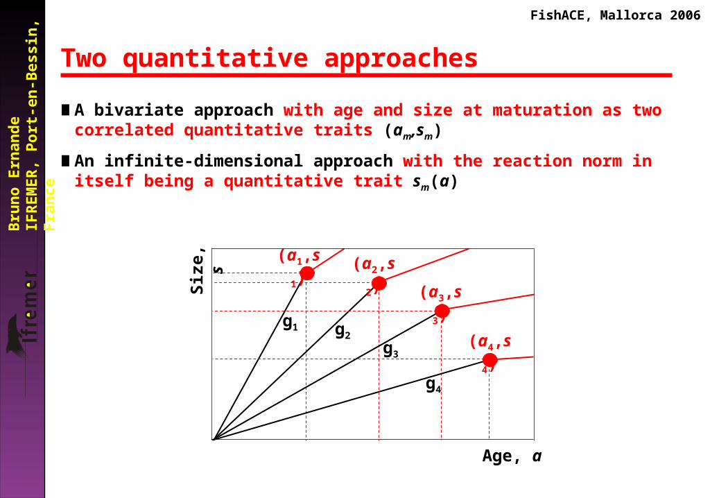
Two quantitative approaches

∎ A bivariate approach with age and size at maturation as two correlated quantitative traits (am,sm)

∎ An infinite-dimensional approach with the reaction norm in itself being a quantitative trait sm(a)

Age, a

Size

, s

g1

(a1,s1)

g2

(a2,s2)

g3

(a3,s3)

g4

(a4,s4)


runo

Ern

ande

IFR

EMER

, Por

t-en-

Bes

sin,

Fra

nce




Age, a

Size

, s


runo

Ern

ande

IFR

EMER

, Por

t-en-

Bes

sin,

Fra

nce




Age, a

Size

, s sm(a)


runo

Ern

ande

IFR

EMER

, Por

t-en-

Bes

sin,

Fra

nce

Bivariate phenotype : the basic model

m

m ijkl

a

s

g gr ei j k

interactions

g gr g e gr e g gr ei j i k j k i j k

igkl

micro-environment

genotypegrowth

environment beyond growth

Individualphenotype


runo

Ern

ande

IFR

EMER

, Por

t-en-

Bes

sin,

Fra

nce

Bivariate phenotype : (co)variance components

Zm

genotypegrowth

environment beyond growth

Phenotypicvariance

G GR G E GR E G GR Ek k k

G GR Ek

micro-environment

interactions


runo

Ern

ande

IFR

EMER

, Por

t-en-

Bes

sin,

Fra

nce

What can we extract using the bivariate approach?

)( 1gam )( 2gam )( 3gam )( 3gsm)( 2gsm)( 1gsm

Distribution of age at maturation conditional on growth

Distribution of size at

maturation conditional on

growth


runo

Ern

ande

IFR

EMER

, Por

t-en-

Bes

sin,

Fra

nce

What can we extract using the bivariate approach?

∎ The growth-related environmental (co)variance can be estimated as the (co)variance of the mean age and size at maturation conditional to growth

―

∎ The distribution of age and size at maturation can be averaged over growth rates, which gives access to an upward biased estimate of genetic (co)variance,

―

∎ An upward biased estimate of the variance related to the genotype-growth interaction can be obtained by substracting the twoi previous estimates from total phenotypic variance,

―

G Ε G Ek k

GR

G GR GR E G GR Ek k


runo

Ern

ande

IFR

EMER

, Por

t-en-

Bes

sin,

Fra

nce

Infinite-dimensional phenotype: the basic model

m i k iklikla a a a g es

genotypeenvironment beyond growth

micro-environment

Individualphenotype


runo

Ern

ande

IFR

EMER

, Por

t-en-

Bes

sin,

Fra

nce

Infinite-dimensional phenotype: variance components

m ka a a a ES G

genotypeenvironment beyond growth

micro-environment

Phenotypicvariance


runo

Ern

ande

IFR

EMER

, Por

t-en-

Bes

sin,

Fra

nce

What can we extract using the infinite-dimensional approach?

4

5

6

730

50

80

40

60

70

0.000.250.500.751.00

Age, a

Size

, s

Probability of maturing


runo

Ern

ande

IFR

EMER

, Por

t-en-

Bes

sin,

Fra

nce


4

5

6

7 30

50

80

40

60

70

Age, a

Size

, s

freq

uenc

y

The whole distribution of age and size at maturation can be inferred from the probabilistic maturation reaction norm


runo

Ern

ande

IFR

EMER

, Por

t-en-

Bes

sin,

Fra

nce


∎ Since the effect of growth is already removed in the infinite-dimensional approach, the phenotypic variance of the infinite-dimensional approach is already an upward biased estimate of genetic variance

― m ka a a a S G E


runo

Ern

ande

IFR

EMER

, Por

t-en-

Bes

sin,

Fra

nce

What are future needs of research?

∎ The coefficient of relatedness between individuals is needed to obtain unbiased estimates of

―

―

∎ Classical quantitative genetics experiments with controlled mating designAdvantage: high statistical powerDisadvantages:

― long experiments (maturity of most commercially exploited fish occurs late in life), ― experimental environmental variation might be not representative of natural

environmental variation

aGG G GR ,


runo

Ern

ande

IFR

EMER

, Por

t-en-

Bes

sin,

Fra

nce

What are future needs of research?

∎ Using micro-satellites to determine the coefficient of relatedness between individuals in the wild

Advantage:― representative of natural environmental variation― information available immediately

Disadvantages: ― is it possible?,― low statistical power


runo

Ern

ande

IFR

EMER

, Por

t-en-

Bes

sin,

Fra

nce

6. Quantitative genetic modelsof evolutionary dynamics


runo

Ern

ande

IFR

EMER

, Por

t-en-

Bes

sin,

Fra

nce

Response to selection


runo

Ern

ande

IFR

EMER

, Por

t-en-

Bes

sin,

Fra

nce

The breeder’s equation: Response to selection (Falconer, 1960)

∎ Response to selection seen through the parent-offspring regression

μo*/μp* = βop’

μo* = βop’ μp* = V(a) μp*/ V(zp)

mid-parent

offspring

μo*

μp*


runo

Ern

ande

IFR

EMER

, Por

t-en-

Bes

sin,

Fra

nce


∎ Principle:

z

Freq

uenc

y

μz(n) μz*(n) μz(n+1)μz(n)

Generation n Generation n+1

z


runo

Ern

ande

IFR

EMER

, Por

t-en-

Bes

sin,

Fra

nce


∎ Principle:

∎ Equation:

z

Freq

uenc

y

μz(n) μz*(n) μz(n+1)μz(n)

Generation n Generation n+1

Selectiondifferential, s

Heritability, h2

az z z z

z

n n n n2

*2

( 1) ( ) ( ( ) ( ))

z


runo

Ern

ande

IFR

EMER

, Por

t-en-

Bes

sin,

Fra

nce


∎ Equation:

Selection gradient, β

z zz z

n nn n V a

V z

*( ( ) ( ))( 1) ( ) ( )

( )


runo

Ern

ande

IFR

EMER

, Por

t-en-

Bes

sin,

Fra

nce


∎ Equation:

∎ Selection differential s, intensity of selection i and selection gradient β

s = (μz(n)-μz*(n)) = i σz

β = s/ V(z) = i/σz


z zz z

n nn n V a

V z

*( ( ) ( ))( 1) ( ) ( )

( )


runo

Ern

ande

IFR

EMER

, Por

t-en-

Bes

sin,

Fra

nce


∎ Equation:

∎ Selection differential s, intensity of selection i and selection gradient β

s = (μz(n)-μz*(n)) = i σz

β = s/ V(z) = i/σz

∎ Recasting the breeder’s equation

Δμz = h2s = V(a)β = V(a)i/σz


z zz z

n nn n V a

V z

*( ( ) ( ))( 1) ( ) ( )

( )


runo

Ern

ande

IFR

EMER

, Por

t-en-

Bes

sin,

Fra

nce

The breeder’s equation: Natural selection (Lande, 1976)

∎ The breeder’s equation was derived for the purpose of artificial selection. In case of natural selection, the selection gradient has to be derived from fitness W(z) and the distribution of phenotypes p(z,n)


runo

Ern

ande

IFR

EMER

, Por

t-en-

Bes

sin,

Fra

nce



∎Mean phenotype

z n zp z n z( ) ( , )d


runo

Ern

ande

IFR

EMER

, Por

t-en-

Bes

sin,

Fra

nce



∎Mean phenotype

∎Mean fitness

z n zp z n z( ) ( , )d

W p z n W z z( , ) ( )d


runo

Ern

ande

IFR

EMER

, Por

t-en-

Bes

sin,

Fra

nce



∎Mean phenotype

∎Mean fitness

∎Mean phenotype after natural selection

z n zp z n z( ) ( , )d

W p z n W z z( , ) ( )d

z n zp z n W z zW

* 1( ) ( , ) ( )d


runo

Ern

ande

IFR

EMER

, Por

t-en-

Bes

sin,

Fra

nce



∎Mean phenotype

∎Mean fitness

∎Mean phenotype after natural selection

∎ Phenotypes’ distribution

z n zp z n z( ) ( , )d

W p z n W z z( , ) ( )d

z

zz

z np z n

2

22

2( ( ))1( , ) exp( )

22

z n zp z n W z zW

* 1( ) ( , ) ( )d


runo

Ern

ande

IFR

EMER

, Por

t-en-

Bes

sin,

Fra

nce


∎Mean fitness derivative

z z zz z

W p z nW z z W n n

n n2 *( , )

( )d ( / )( ( ) ( ))( ) ( )


runo

Ern

ande

IFR

EMER

, Por

t-en-

Bes

sin,

Fra

nce



∎ Breeder’s equation under natural selection

Note that fitness is here frequency-independent.

zz z

V a W WV a

W n n

( ) ln( )

( ) ( )

z z zz z

W p z nW z z W n n

n n2 *( , )

( )d ( / )( ( ) ( ))( ) ( )


runo

Ern

ande

IFR

EMER

, Por

t-en-

Bes

sin,

Fra

nce



∎ Breeder’s equation under natural selection

Note that fitness is here frequency-independent.

∎ Extension to the frequency-dependent case

zz z

V a W WV a

W n n

( ) ln( )

( ) ( )

z z zz z

W p z nW z z W n n

n n2 *( , )

( )d ( / )( ( ) ( ))( ) ( )

zz z

V a W W zp z n z

W n n

( ) ( )( ( , ) d )

( ) ( )


runo

Ern

ande

IFR

EMER

, Por

t-en-

Bes

sin,

Fra

nce

Multivariate evolution: Dynamics (Lande, 1979)

∎ The breeder’s equation can be generalized to multivariate phenotypes

with

W1zμ AZ s Aβ A ln

m

W

z

W

W

z

1

ln

ln ...

ln


runo

Ern

ande

IFR

EMER

, Por

t-en-

Bes

sin,

Fra

nce

Multivariate evolution: Dynamics (Lande, 1979)

∎ The breeder’s equation can be generalized to multivariate phenotypes

with

∎ In other words, the evolution of a particular character i is given by

with Aij the additive genetic covariance between trait i and j

m

W

z

W

W

z

1

ln

ln ...

ln

i j

m

z ij zj i

A Wln /

W1zμ AZ s Aβ A ln


runo

Ern

ande

IFR

EMER

, Por

t-en-

Bes

sin,

Fra

nce

Multivariate evolution: Genetic constraints (Lande, 1979)

∎ Evolutionary dynamics may come to a halt becauseThe selection gradient vanishes

for all zi

The additive genetic co-variance matrix is singular, so that

whatever the selection gradient

WA ln 0

izWln / 0

Wln


runo

Ern

ande

IFR

EMER

, Por

t-en-

Bes

sin,

Fra

nce



for all zi



∎ The rate and direction of evolution determined by the selection gradient are modified by the genetic co-variance matrix. The rate of evolution of a given trait is a sum of

the response to direct selection on that trait and the correlated responses to selection on genetically correlated traits

WA ln 0

izWln / 0

Wln


runo

Ern

ande

IFR

EMER

, Por

t-en-

Bes

sin,

Fra

nce



for all zi



∎ The rate and direction of evolution determined by the selection gradient are modified by the genetic co-variance matrix. The rate of evolution of a given trait is a sum of

the response to direct selection on that trait and the correlated responses to selection on genetically correlated traits

∎ Genetic constraintsLack of genetic variance: The rate of response to direct selection is scaled by the additive genetic

varianceTrade-offs: the rate and direction of responses to correlated selection depends on additive

genetic covariance with other traits, so that the direction may be opposite to the actual force of selection thus highlighting trade-offs between traits

WA ln 0

izWln / 0

Wln


runo

Ern

ande

IFR

EMER

, Por

t-en-

Bes

sin,

Fra

nce

Advantage and drawbacks

∎ Quantitative genetic evolutionary dynamicsallow studying both genetic and phenotypic evolution,

predict both evolutionary transient states and equilibrium

accounts for genetic constraints such as the lack of variance or trade-offs

∎ Drawbacksno detailed ecological considerations or population dynamics: fitness and selection gradient are

not extracted from the ecological setting

― not geared toward identifying explicit selective pressures,

― no complex population dynamics and frequency-dependent selection

constant additive genetic variance-covariance matrices: limited to short term evolution or “weak” selection, so that the mutation-selection balance can maintain additive genetic (co-)variance (Lande 976, 1979).

bruno ernande ifremer, port-en-bessin, france fishace, mallorca 2006 quantitative genetics: analysis...

Documents

bruno ernande ifremer

france fishace

france slide

qg analysis of phenotypes

genotypic variation

partitioning genotypic

genotypic values g

partitioning phenotypes