bringing stability to wireless mesh networks - infoscience - epfl
TRANSCRIPT

Abstract
Wireless mesh networks were designed as a mean to rapidly deliver large-scalecommunication capabilities without the support of any prior infrastructure. Amongthe different properties of mesh networks, the self-organizing featureis particularlyinteresting for developing countries or for emergency situations. However, thesebenefits also bring new challenges. For example, the scheduling decision needsto be performed in a distributed manner at each node of the network. Toward thisgoal, most of the current mesh deployments are based on the IEEE 802.11 protocol,even if it was not designed for multi-hop communications.
The main goals of this thesis are (i) to understand and model the behaviorof IEEE 802.11-based mesh networks and more specifically the root causes thatlead to congestion and network instability; (ii) to develop an experimental infras-tructure in order to validate with measurements both the problems and the solu-tions discussed in this thesis; (iii) to build efficient hop-by-hop scheduling schemesthat provide congestion control and inter-flow fairness in a practical way and thatare backward-compatible with the current protocol; and (iv) to explain thenon-monotonic relation between the end-to-end throughput and the source rateand tointroduce a model to derive the rationale behind this artifact.
First, we propose a Markovian model and we introduce the notion ofstealingeffectto explain the root causes behind the3-hop stability boundary, where linearnetworks up to3 hops are stable, and larger topologies are intrinsically unstable.We validate our analytical results both through simulations and through measure-ments on a small testbed deployment.
Second, to support the experimental research presented in this thesis, we designand deploy a large-scale mesh network testbed on the EPFL campus. We planourarchitecture to be as flexible as possible in order to support a wide range of otherresearch areas such as IEEE 802.11 indoor localization and opportunistic routing.
Third, we introduceEZ-flow, a novel hop-by-hop congestion-control mecha-nism that operates at the Medium Access Control layer. EZ-flow is fully backward-compatible with the existing IEEE 802.11 deployments and it works without anyform of message passing. To perform its task EZ-flow takes advantage of the broad-cast nature of the wireless medium in order to passively derive the queuesize atthe next-hop node. This information is then used by each node to adapt accord-ingly its channel access probability, through the contention window parameter ofIEEE 802.11. After detailing the different components of EZ-flow, we analyze its
i
performance analytically, through simulations and real measurements.Fourth, we show that hop-by-hop congestion-control can be efficiently per-
formed at the network layer in order to not abuse the contention mechanism ofIEEE 802.11. Additionally, we introduce a complete framework that jointly achievescongestion-control and fairness without requiring a prior knowledge of the networkcapacity region. To achieve the fairness part, we propose theExplore & Enhancealgorithm that finds a fair and achievable rate allocation vector that maximizes adesired function of utility. We show experimentally that this algorithm reachesits objective by alternating between exploration phases (to discover the capacityregion) and enhancement phases (to improve the utility through a gradient ascent).
Finally, we note that, as opposed to wired networks, the multi-hop wirelesscapacity is usually unknown and time-varying. Therefore, we study how the end-to-end throughput evolves as a function of the source rate when operating bothbelowandabovethe network capacity. We note that this evolution follows a non-monotonic curve and we explain, through an analytical model and simulations,therationale behind the different transition points of this curve. Following our anal-ysis, we show that no end-to-end congestion control can be throughput-optimal ifit operates directly over IEEE 802.11. Hence, this supports the methodology ofperforming congestion control in a hop-by-hop manner. After validating experi-mentally the non-monotonicity, we compare through simulations different state-of-the-art scheduling schemes and we highlight the important tradeoff thatexistsin congestion-control schemes betweenefficiency(i.e., throughput-optimality) androbustness(i.e., no throughput collapse when the sources attempt to operate at arate above the network capacity).
Keywords
Wireless mesh networks, multi-hop networks, IEEE 802.11, scheduling, mediumaccess control, congestion control, network stability, modeling, implementation,experimental measurements, testbed deployment.
ii

Resume
Les reseaux mailles sans fil ontete concus afin de permettre le deploiement rapided’un moyen de communication, et cela sans necessiter le soutien d’une infrastruc-ture preexistante. Parmi les avantages offerts par ces reseaux, l’auto-organisationsemble particulierement interessante dans le cas de deploiements dans des paysemergents ou en situation de catastrophes naturelles. Cependant, ces avantages neviennent pas sans nouveaux defis. Par exemple, la planification d’acces au canaldoit etre effectuee de maniere distribuee. La plupart des deploiements de reseauxmailles sans fil actuels realisent cela en utilisant le standard IEEE 802.11, meme sice protocole n’a pasete concu pour des communicationsa sauts multiples.
Les principaux objectifs de cette these sont (i) de comprendre et de modeliserle comportement des reseaux mailles sans fil bases sur IEEE 802.11, en se concen-trant sur les facteurs cles qui conduisenta l’instabilite et la congestion du reseau;(ii) de developper un reseau sans fil experimental afin de valider avec des mesuresreelles les problemes et les solutions presentes dans cette these; (iii) de proposer desmethodes de planification d’acces au canal qui offrent simultanement un controlede congestion efficace et une forme d’equite entre les differents flux presents dansle reseau; et (iv) de souligner la non-monotonicite de la relation entre le debit debout-en-bout et le debit recua la source, puis de proposer un modele analytiquepour en expliquer les raisons.
Dans un premier temps, nous proposons un modele Markovien et nous intro-duisons la notion d’effet de ‘detournement’pour expliquer les causes menanta lalimite de stabilite de3 sauts. Cette limite se manifeste par la stabilite des reseauxlineaires jusqu’a 3 sauts, en oppositiona l’instabilite intrinseque de plus grandestopologies. Nous validons nos resultats analytiques aussi bien par des simulationsque par des mesures sur un reseau maille a petiteechelle.
Dans un deuxieme temps, nous concevons et deployons un reseau maille sansfil a grandeechelle au sein du campus de l’EPFL. Nous planifions l’architecture dureseau afin qu’elle soit la plus flexible possible et qu’elle puisse soutenir unlargeeventail de themes de recherche tels que la localisation basee sur IEEE 802.11 etle routage opportuniste.
Dans un troisieme temps, nous proposonsEZ-flow, un nouveau mecanisme decontrole de congestion lien-par-lien qui fonctionne au niveau de la couche MAC.EZ-flow est entierement retro-compatible avec les protocoles existants bases surIEEE 802.11 et il fonctionne sansechange de messages de controle entre les nœuds.
iii
Ce mecanisme tire parti de la nature diffusive du support sans fil: il calcule ainsipassivement la taille de la file du nœud suivant. Chaque nœud utilise ensuite cetteinformation pour adapter sa probabilite d’acces au canal, en modifiant la taille dela fenetre de contention de IEEE 802.11. Pour finir, nous analysons les perfor-mances du mecanisme EZ-flow en nous appuyant sur des resultats analytique, dessimulations, et de mesures reelles.
Dans un quatrieme temps, nous montrons que le controle de congestion lien-par-lien peutetre effectue de maniere tout aussi efficace au niveau de la couchereseau, afin de ne pas denaturer le mecanisme se chargeant du controle de con-tention dans le protocole IEEE 802.11. En outre, nous developpons une solu-tion qui offre conjointement un controle de congestion et une forme d’equite en-tre les flux. Tout ceci est realise sans necessiter la connaissance prealable de laregion de capacite du reseau. Afin de fournir une forme d’equite, nous proposonsl’algorithme Explore & Enhance. Cet algorithme trouve un vecteur d’allocationdes debits realisable maximisant une fonction d’utilite donnee. Nous montronsexperimentalement que ce mecanisme atteint cet objectif en alternant entre (i)des phases d’exploration afin decouvrir la region de capacite et (ii) des phasesd’amelioration qui font croitre l’utilite gracea une montee de gradient.
Finalement, nous notons que, contrairement aux reseaux cables, la capacite desreseaux sans fila sauts multiples est generalement non seulement inconnue, maisaussi variable dans le temps. Il est donc primordial d’etudier l’evolution du debitde bout-en-bout du reseau lorsque l’on fait varier le debit recu par les sources (aussibienen dessouset qu’au dessusde la capacite du reseau). Nous remarquons quecetteevolution est non monotone et expliquons les raisons de ce comportementen nous appuyant sur un modele analytique et des simulations. Suitea la valida-tion experimentale de ce phenomene, nous montrons qu’il est impossible pour unmecanisme de controle de congestion fonctionnant de bout-en-bout d’atteindre ledebit optimal si le protocole IEEE 802.11 est utilise au niveau MAC. Cela soutientl’id ee qu’un controle de congestion efficace doit s’effectuer lien-par-lien. Nousnous concentrons donc sur les differents mecanismes lien-par-lien et comparonsleur performance, ce qui met enevidence l’importance du compromis qui existeentreefficacite (optimalite du debit) etrobustesse(pas de chute du debit lorsque laquantite de trafic recu par les sources est superieurea la capacite du reseau).
Mots cles
Reseaux mailles sans fil, reseauxa sauts multiples, IEEE 802.11, protocole degestion d’acces au canal, protocole de controle de congestion, stabilite des reseaux,modelisation, implementation, mesures experimentales, deploiement de reseaux.
iv
Acknowledgments
I would like to thank my advisor Prof. Patrick Thiran for accepting me in hisresearch group and for making this PhD such an enriching experience,both on apersonal and a scientific level. I really appreciated his sense of scientificrigor andthe freedom he gave me in exploring my own research interests.
In addition, I want to thank Sylviane Dal Mas for informing me about thisPhD opportunity and for all her hard work she does to make the CommunicationSystems Section such a great department to study in. A special thank goes alsoto Dr. Roger Karrer from Deutsche Telekom Laboratories for having launchedthe MagNets project that mainly funded my research work. While working withhim, I learned a lot from his experience in system research and this was a valuablecomplement to the more theoretical approach I acquired at EPFL.
It was a great pleasure and a humbling experience to have Prof. Martin Hasler,Prof. Jean-Pierre Hubaux, Dr. Konstantina Papagiannaki, and Prof. David Starobin-ski in my jury. I want to thank them for accepting to review this thesis.
Next, I would like to thank all the people with whom I had the opportunity tocollaborate during my PhD research, in particular Dr. Alaeddine El Fawal,JulienHerzen, Dr. Ruben Merz, and Dr. Seva Shneer. I also want to thank all my EPFLcolleagues for making this place such a lively environment.
I am also very thankful to the lab’s staff for their support and enthusiasm.Thanks to Holly Cogliati for all her advice in English and for the dedication sheshowed in reviewing and helping me to improve the clarity of most of my publica-tions. Thanks to Danielle Alvarez, Angela Devenoge, and Patricia Hjelt formak-ing all the administrative processes go smoothly. Thanks to Herve Chabanel, YvesLopes, Marc-Andre Luthi, and Richard Timsit for letting me deploy my multi-hoptestbed on the campus and for their support and advice.
Finally, I thank my parents for always being there for me and for the supportand care they gave to me throughout my studies. I thank all my friends for makingthis PhD time a nice period of my life. In particular I thank Raphael and Mohamedfor pushing me to keep the right balance between work and sports. And last but notleast, I am really thankful to Mutunge for the precious support she gaveme and forall the great moments we shared together during my PhD experience.
v

vi
Contents
1 Introduction 11.1 Motivation . . . . . . . . . . . . . . . . . . . . . . . . . . . . . . 11.2 Dissertation Outline . . . . . . . . . . . . . . . . . . . . . . . . . 31.3 Contributions . . . . . . . . . . . . . . . . . . . . . . . . . . . . 5
2 Background 72.1 Wireless Mesh Networks . . . . . . . . . . . . . . . . . . . . . . 72.2 The Layer Model . . . . . . . . . . . . . . . . . . . . . . . . . . 92.3 The IEEE 802.11 Protocol . . . . . . . . . . . . . . . . . . . . . 10
2.3.1 Description in Single-Hop Environments . . . . . . . . . 112.3.2 Challenges in Multi-Hop Environments . . . . . . . . . . 122.3.3 IEEE 802.11s . . . . . . . . . . . . . . . . . . . . . . . . 14
2.4 Desired Properties of Mesh Networks . . . . . . . . . . . . . . . 14
3 Modeling the Instability of Mesh Networks 173.1 Background . . . . . . . . . . . . . . . . . . . . . . . . . . . . . 17
3.1.1 Problem Statement . . . . . . . . . . . . . . . . . . . . . 173.1.2 Related Work . . . . . . . . . . . . . . . . . . . . . . . . 19
3.2 Analytical Model . . . . . . . . . . . . . . . . . . . . . . . . . . 203.2.1 MAC Layer Description . . . . . . . . . . . . . . . . . . 203.2.2 Discrete Markov Chain Model . . . . . . . . . . . . . . . 203.2.3 Stealing Effect Phenomenon . . . . . . . . . . . . . . . . 223.2.4 Stability Definition . . . . . . . . . . . . . . . . . . . . . 23
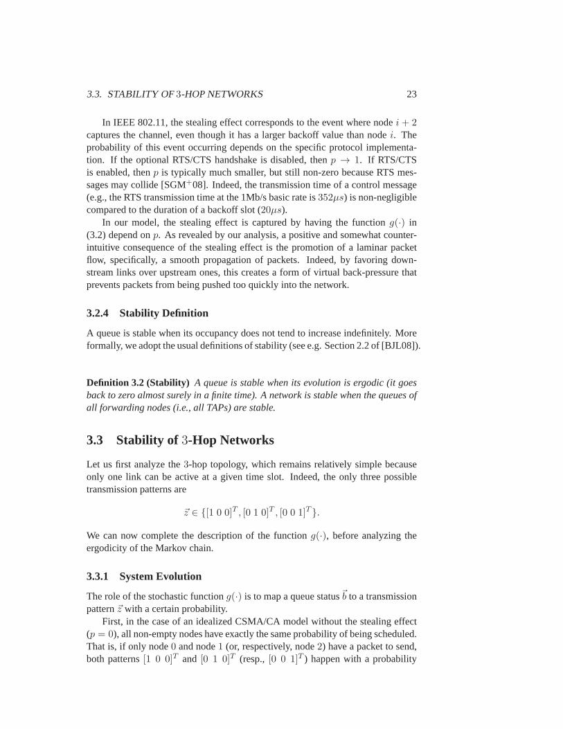
3.3 Stability of3-Hop Networks . . . . . . . . . . . . . . . . . . . . 233.3.1 System Evolution . . . . . . . . . . . . . . . . . . . . . . 233.3.2 Stability Analysis . . . . . . . . . . . . . . . . . . . . . . 25
3.4 Instability of4-Hop Networks . . . . . . . . . . . . . . . . . . . 273.4.1 System Evolution . . . . . . . . . . . . . . . . . . . . . . 273.4.2 Stability Analysis . . . . . . . . . . . . . . . . . . . . . . 303.4.3 Extension to LargerK-Hop Topologies . . . . . . . . . . 32
3.5 Static Stabilization Strategy . . . . . . . . . . . . . . . . . . . . . 333.5.1 Source Throttling . . . . . . . . . . . . . . . . . . . . . . 333.5.2 Penalty Model . . . . . . . . . . . . . . . . . . . . . . . 34
vii
3.5.3 Theoretical Analysis . . . . . . . . . . . . . . . . . . . . 353.5.4 Experimental Analysis . . . . . . . . . . . . . . . . . . . 36
3.6 Simulations on Multi-Flow Topologies . . . . . . . . . . . . . . . 373.7 Instability Problem at Higher Rates . . . . . . . . . . . . . . . . . 393.8 Concluding Remarks . . . . . . . . . . . . . . . . . . . . . . . . 42
4 Building an Indoor Wireless Testbed 434.1 Problem Statement . . . . . . . . . . . . . . . . . . . . . . . . . 434.2 Choice of Hardware and Software . . . . . . . . . . . . . . . . . 44
4.2.1 Requirements and Challenges . . . . . . . . . . . . . . . 444.2.2 Hardware Description . . . . . . . . . . . . . . . . . . . 454.2.3 OpenWRT Firmware . . . . . . . . . . . . . . . . . . . . 474.2.4 MadWiFi Driver . . . . . . . . . . . . . . . . . . . . . . 47
4.3 Testbed Deployment . . . . . . . . . . . . . . . . . . . . . . . . 484.3.1 Topology . . . . . . . . . . . . . . . . . . . . . . . . . . 484.3.2 Network Control Tool . . . . . . . . . . . . . . . . . . . 49
4.4 Concluding Remarks . . . . . . . . . . . . . . . . . . . . . . . . 53
5 MAC Layer Congestion-Control 555.1 Background . . . . . . . . . . . . . . . . . . . . . . . . . . . . . 55
5.1.1 Problem Statement . . . . . . . . . . . . . . . . . . . . . 555.1.2 System Requirements . . . . . . . . . . . . . . . . . . . 565.1.3 Related Work . . . . . . . . . . . . . . . . . . . . . . . . 57
5.2 EZ-Flow: a Scheme without Message Passing . . . . . . . . . . . 595.2.1 EZ-Flow Description . . . . . . . . . . . . . . . . . . . . 595.2.2 Buffer Occupancy Estimation . . . . . . . . . . . . . . . 605.2.3 Channel Access Adaptation . . . . . . . . . . . . . . . . 62
5.3 Experimental Evaluation . . . . . . . . . . . . . . . . . . . . . . 645.3.1 Hardware and Software Description . . . . . . . . . . . . 645.3.2 Topology Description . . . . . . . . . . . . . . . . . . . . 655.3.3 Measurement Results . . . . . . . . . . . . . . . . . . . . 665.3.4 Effect of Bi-Directional Traffic . . . . . . . . . . . . . . . 68
5.4 Simulation Results . . . . . . . . . . . . . . . . . . . . . . . . . 705.4.1 System Description . . . . . . . . . . . . . . . . . . . . . 705.4.2 Scenario 1:2-Flow Topology . . . . . . . . . . . . . . . 715.4.3 Scenario 2:3-Flow Topology . . . . . . . . . . . . . . . 74
5.5 Dynamical Model . . . . . . . . . . . . . . . . . . . . . . . . . . 775.5.1 EZ-Flow Dynamics . . . . . . . . . . . . . . . . . . . . . 775.5.2 Proof of Stability . . . . . . . . . . . . . . . . . . . . . . 78
5.6 Concluding Remarks . . . . . . . . . . . . . . . . . . . . . . . . 81
viii

6 Joint Congestion-Control and Fairness 836.1 Background . . . . . . . . . . . . . . . . . . . . . . . . . . . . . 83
6.1.1 Problem Statement . . . . . . . . . . . . . . . . . . . . . 836.1.2 System Model and Assumptions . . . . . . . . . . . . . . 856.1.3 Related Work . . . . . . . . . . . . . . . . . . . . . . . . 87
6.2 Intra-Flow Congestion Control . . . . . . . . . . . . . . . . . . . 896.3 Inter-Flow Fairness . . . . . . . . . . . . . . . . . . . . . . . . . 91
6.3.1 Model Description . . . . . . . . . . . . . . . . . . . . . 926.3.2 Algorithm Description . . . . . . . . . . . . . . . . . . . 93
6.4 Joint Congestion Control and Fairness for WMNs . . . . . . . . . 956.5 Experimental Evaluation . . . . . . . . . . . . . . . . . . . . . . 96
6.5.1 Hardware and Software Description . . . . . . . . . . . . 966.5.2 Evaluation of the Intra-Flow Congestion Control . . . . . 976.5.3 Evaluation of the Inter-Flow Fairness . . . . . . . . . . . 986.5.4 Evaluation of the Complete Framework . . . . . . . . . . 100
6.6 Concluding Remarks . . . . . . . . . . . . . . . . . . . . . . . . 101
7 Multi-Hop Networks Beyond Capacity 1037.1 Background . . . . . . . . . . . . . . . . . . . . . . . . . . . . . 103
7.1.1 Problem Statement . . . . . . . . . . . . . . . . . . . . . 1037.1.2 Related Work . . . . . . . . . . . . . . . . . . . . . . . . 1057.1.3 Network Model . . . . . . . . . . . . . . . . . . . . . . . 106
7.2 Simulations . . . . . . . . . . . . . . . . . . . . . . . . . . . . . 1077.2.1 4-Hop Networks . . . . . . . . . . . . . . . . . . . . . . 1077.2.2 5-Hop Networks . . . . . . . . . . . . . . . . . . . . . . 1087.2.3 Larger K-Hop Networks . . . . . . . . . . . . . . . . . . 109
7.3 Mathematical Analysis . . . . . . . . . . . . . . . . . . . . . . . 1107.3.1 4-Hop Network . . . . . . . . . . . . . . . . . . . . . . . 110
7.4 Experimental Validation . . . . . . . . . . . . . . . . . . . . . . 1157.4.1 Topology Description . . . . . . . . . . . . . . . . . . . . 1157.4.2 Measurement Results . . . . . . . . . . . . . . . . . . . . 116
7.5 Hop-by-Hop Congestion Control . . . . . . . . . . . . . . . . . . 1177.6 Concluding Remarks . . . . . . . . . . . . . . . . . . . . . . . . 121
8 Conclusion 1238.1 Discussion of the Results . . . . . . . . . . . . . . . . . . . . . . 1238.2 Possible Extensions . . . . . . . . . . . . . . . . . . . . . . . . . 125
A Useful Theorems 129A.1 Foster’s Theorem . . . . . . . . . . . . . . . . . . . . . . . . . . 129A.2 Transcience Theorem . . . . . . . . . . . . . . . . . . . . . . . . 129A.3 Non-ergodicity Theorem . . . . . . . . . . . . . . . . . . . . . . 130
ix
B Mesh How-To Guide 131B.1 Building, Installing and Configuring OpenWRT . . . . . . . . . . 131
B.1.1 Getting the Source and Compiling on Your Computer . . . 131B.2 Extending OpenWRT with Some Useful Packages . . . . . . . . . 137
B.2.1 Basics for Adding a Package on your Router . . . . . . . 138B.2.2 Adding the Click Modular Router . . . . . . . . . . . . . 138B.2.3 Adding 802.1x Support for a Secure Wired Connection . . 139B.2.4 Adding your Own Program/Package . . . . . . . . . . . . 141B.2.5 Cross-compiling your Program without Making a Package 143
B.3 Hacking the MadWiFi Driver . . . . . . . . . . . . . . . . . . . . 143B.3.1 Unlocking the Modification of MAC Parameters . . . . . 143B.3.2 Enabling MadWifi to Announce the FULLBUFFER Sta-
tus to Upper Layers . . . . . . . . . . . . . . . . . . . . . 143B.3.3 Adding New Commands to Access MAC Parameters . . . 144
B.4 Installing and Using Net-Controller . . . . . . . . . . . . . . . . 145B.4.1 Installation . . . . . . . . . . . . . . . . . . . . . . . . . 145B.4.2 Configuration . . . . . . . . . . . . . . . . . . . . . . . . 145B.4.3 Using the Graphical Interface . . . . . . . . . . . . . . . 147
Publications 151
Curriculum Vitæ 153
Bibliography 154
x

Chapter 1
Introduction
1.1 Motivation
Wireless Mesh Networks (WMNs) have received increasing attention since theirintroduction in 1994 under the name ofmassive array cellular systems[Pie94].Initially, they were intended to be a cost-effective alternative to replace thelast-mile infrastructure of large metropolitan cities. Examples of such deploymentstook place in cities such as San Francisco, where Meraki deployed a city-widewireless mesh network in 2008. To realize this project, Meraki used around 10,000-15,000 indoor nodes and a few hundred solar-powered outdoor nodes [Fle08]. Thistype of successful commercial deployment shows that WMNs have the potential todeliver large-scale broadband connectivity to metropolitan areas. Nevertheless, dueto widely available wired broadband connectivity, the utility of mesh networks hasproved to be superfluous in developed countries. Consequently, mesh networks arenow seen as an efficient way to quickly provide connectivity in uncovered areas,such as in developing countries or in emergency situations after a natural disaster,for example.
An example for the case of developing countries is theOne Laptop per Childproject launched in 2005 [OLP]. The goal of this project is to provide educationalopportunities to the world’s poorest children by giving them a low-cost and low-powered laptop with dedicated software. To reach this objective, a laptop namedXO was designed. As this laptop is likely to be used in regions where little com-munication infrastructure exists, it relies on the wireless mesh network technologyin order to provide a form of connectivity between the different machines.
Emergency situations can arise both in developing and developed countries.Indeed, different external factors could disrupt the smooth operationof the net-work. In the case of natural disasters, such as earthquakes or tsunamis, the wiredinfrastructure could be physically damaged thus preventing traditional communi-cations from taking place. This lack of connectivity does not allow the rescueteams to efficiently synchronize, which leads to dramatic consequences in emer-gency situations, where every minute counts to save human lives. WMNs provide
1

2 CHAPTER 1. INTRODUCTION
a serious solution to these situations as they allow for the rapid deployment ofan operational network without relying on any pre-existing infrastructure. More-over, recent events in Egypt have shown that connectivity can be shut down, evenin the presence of a fully operational infrastructure. Indeed, during the Egyptianrevolution of January 2011, the government reacted by disconnecting the wholecountry from Internet and switching off cellular communications. This communi-cation blackout is an attack against freedom that could lead to chaos in the streets.The striking fact in this specific situation is that this country-wide blackout wasrelatively easy to perform for the government. This perfectly illustrates thevulner-ability of the centralized communication technologies that we currently rely on. Asmentioned in the New York Times [TOF11], wireless mesh networks technologycould be deployed in smartphones and this might be a solution to prevent this typeof connectivity blackout from happening in the future.
In order to not suffer from a single point of failure and to provide a reasonablelevel of robustness to hardware breakdown, mesh networks need to bedecentral-ized. This requirement forces the scheduling decisions to be performed ina dis-tributed manner with the transmission decision made locally at each node. Most ofcurrent WMN deployments rely directly on the IEEE 802.11 protocol to take thescheduling decision at the Medium Access Control (MAC) layer. But IEEE 802.11was designed for single-hop networks and was not envisioned for multi-hop com-munications that significantly differ in nature and lead to new challenges.
In single-hop communications, IEEE 802.11 is widely used and it is the well-accepted standard for wireless local area networks (WLAN) that are largely de-ployed both in homes and offices. The particularity of these networks is thatall thenodes are within the same collision set. This means that at most only one node cansuccessfully transmit at each point in time, and each node can sense whether thechannel is idle or if there is a communication taking place. This single-hop settingof IEEE 802.11 is modeled by Bianchi and he finds that the protocol performs rea-sonably well by delivering good throughput performance together with long-termfairness (short-term fairness is not achieved due to the exponential backoff policyof IEEE 802.11) [Bia00].
Nevertheless, the multi-hop environment is significantly different by nature.Our understanding of the exact behavior of multi-hop IEEE 802.11 networks isstill in its infancy and the existence of relay nodes brings the additional challenge ofcongestion-control. Moreover, measurements from real deployments reflect poorperformance [GSK04] and they lead some researchers to make surprising conclu-sions, such as ”with current commodity wireless technology it does not make senseto handle more than three hops” 1 (we call this finding the3-hop boundaryhere-after). Due to the lack of analytical models capturing the exact dynamics of IEEE802.11 in multi-hop networks, we are still unable to explain the rationale behindsuch a3-hop boundary result and this remains an open issue. Once the causes ofthis problem are understood, the next step would be to design appropriatepractical
1Lunar project: http://cn.cs.unibas.ch/projects/lunar/
1.2. DISSERTATION OUTLINE 3
mechanisms that can overcome this challenge and that remain decentralized andbackward-compatible with existing mesh network deployments.
Finally, we note that as opposed to wired networks, the wireless capacity isusually both unknown and time-varying. Therefore, without being too conserva-tive, it is impossible to guarantee that the source rate is always within the networkcapacity. Yet, most of the recent works on distributed scheduling [SSR09, JWa,PYC08, TE92] focus on the notion of throughput-optimality that ensures that thenetwork is stable for any source ratewithin the capacity region, which is thereforeassumed to be known. This throughput-optimality criterion is useful (it givesameasure ofefficiency), but it does not say anything about the network performanceonce the source rate is above the capacity (it remains clueless aboutrobustness).Therefore, we stress that we really need to clearly understand how the networkperformance (i.e., the throughput) evolves for different source rates, either withinor outside the capacity region. Indeed, an optimal scheduling scheme needs to bebothefficientandrobust.
1.2 Dissertation Outline
We begin by describing the IEEE 802.11 protocol and introducing the notionofwireless mesh networks in Chapter 2. After discussing the fundamental differ-ences between a single-hop and a multi-hop environment, we describe some de-sirable properties of mesh networks, which need to be kept in consideration whendesigning new scheduling schemes.
In order to make it possible to formally study the root causes behind the3-hop boundary (i.e., why is a3-hop network stable, but not a4-hop network), wepropose a Markovian model in Chapter 3. We introduce the notion ofstealingeffect, a consequence of the hidden node problem and of non-zero transmissiondelays, and we discuss its impact on the network stability. After proposing a staticstabilization strategy, we use six off-the-shelf wireless routers in order tovalidateexperimentally both the instability result and the efficiency of our solution.
Because of the importance of experimental validation in the field of mesh net-works and the lack of an experimental platform at our disposal, we decided to buildfrom scratch an experimental multi-hop testbed on the EPFL campus. Our testbedis composed of around60 wireless routers and it spans over the six buildings of theI&C department. In Chapter 4, we review some of the challenges and the practicallessons we learned while building our indoor testbed that was used for ourownresearch work and is still used for various other projects today.
After pointing out the serious stability problem that occurs in wireless multi-hop networks, in Chapter 5 we introduce a practical hop-by-hop congestion-controlscheme calledEZ-flow. EZ-flow is designed to take advantage of the broadcast na-ture of the wireless medium in order for a nodei to passively derive the queue occu-pancy at the next-hopqi+1 without any form of message passing or piggy-backing.Nodei adapts its transmission rate in order to maintain the queueqi+1 stable. We

4 CHAPTER 1. INTRODUCTION
validate the efficiency of EZ-flow in stabilizing the network (i.e., maintaining theend-to-end delay small) both through ns-2 simulations and through measurementsfrom a practical implementation deployed on our indoor testbed.
After tackling the problem of congestion control within a flow at the MAClayer, in Chapter 6 we propose a more complete scheme that runs at the networklayer and that delivers both intra-flow congestion-control and inter-flow fairness.Our distributed solution requires almost no message passing and is completelytransparent to both the MAC (i.e., it does not interact with any parameter of theMAC layer) and the upper layers. First, our network-layer hop-by-hop congestion-control mechanism uses a rate limiter attached to each queue. It adaptively andautomatically adjusts each rate limiter by passively computing the queue size at thenext-hop relay, without any form of message passing. Second, at the mesh gateway,our inter-flow fairness algorithm finds a fair and achievable rate allocationvectorthat maximizes utility without prior knowledge of the capacity region. It runs (i)exploration phases to discover the capacity region and (ii) enhancement phases toimprove the utility by a gradient ascent. Third, both mechanisms smoothly inter-act together to form a complete solution. The fair inter-flow allocation propagatesinto the network using the hop-by-hop intra-flow mechanism and we validate theefficiency of our solution on12 wireless routers of our testbed.
Throughout this thesis, we focus on distributed scheduling schemes that canperform their task without the prior knowledge of the capacity region. As men-tioned earlier, another approach taken by some researchers is to designthroughput-optimal schemes that explicitly require the knowledge of the capacity region in or-der to perform their task. Nevertheless, as opposed to wired networks,the wirelesscapacity is usually unknown and thus it is important to have a clear understand-ing of how the network behaves when the sources are operating eitherbeloworabovethe network capacity. In Chapter 7, we formally study the case of an IEEE802.11 multi-hop network in detail and we explain why the end-to-end through-put is a non-monotonic function of the source rate. Following our simulations andour mathematical study, we prove that it is impossible for an end-to-end conges-tion control scheme to be throughput-optimal if it runs over IEEE 802.11. Thisresult supports the idea of performing congestion-control in a hop-by-hop mannerinstead of end-to-end. Therefore we compare in our simulator differentstate-of-the-art methodologies of performing hop-by-hop congestion control and we showthe important tradeoff between optimality (throughput-optimality) and robustness(no throughput collapse beyond capacity) that should be taken into considerationwhen designing new hop-by-hop scheduling algorithms.
Finally, we conclude this thesis in Chapter 8 with a summary of the main find-ings and a discussion of possible directions for future work.
1.3. CONTRIBUTIONS 5
1.3 Contributions
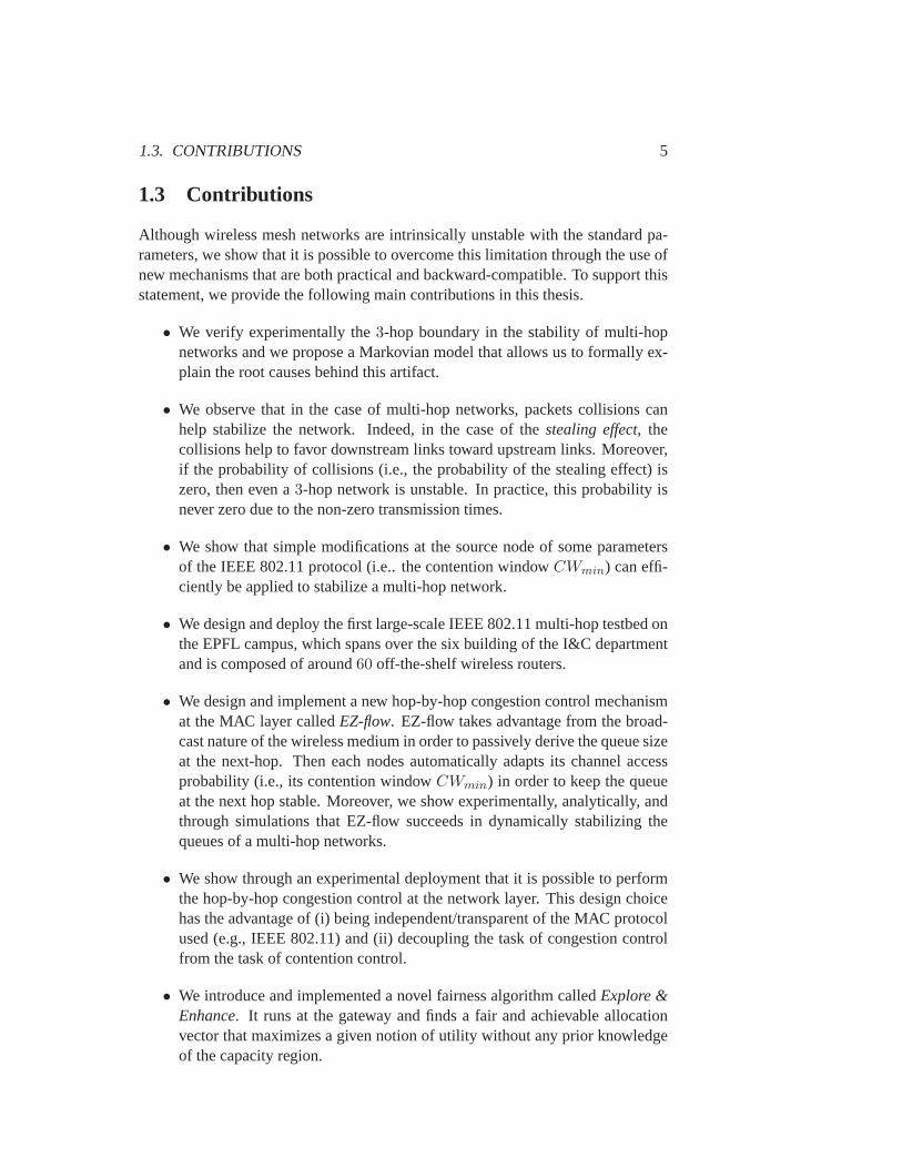
Although wireless mesh networks are intrinsically unstable with the standard pa-rameters, we show that it is possible to overcome this limitation through the use ofnew mechanisms that are both practical and backward-compatible. To support thisstatement, we provide the following main contributions in this thesis.
• We verify experimentally the3-hop boundary in the stability of multi-hopnetworks and we propose a Markovian model that allows us to formally ex-plain the root causes behind this artifact.
• We observe that in the case of multi-hop networks, packets collisions canhelp stabilize the network. Indeed, in the case of thestealing effect, thecollisions help to favor downstream links toward upstream links. Moreover,if the probability of collisions (i.e., the probability of the stealing effect) iszero, then even a3-hop network is unstable. In practice, this probability isnever zero due to the non-zero transmission times.
• We show that simple modifications at the source node of some parametersof the IEEE 802.11 protocol (i.e.. the contention windowCWmin) can effi-ciently be applied to stabilize a multi-hop network.
• We design and deploy the first large-scale IEEE 802.11 multi-hop testbed onthe EPFL campus, which spans over the six building of the I&C departmentand is composed of around60 off-the-shelf wireless routers.
• We design and implement a new hop-by-hop congestion control mechanismat the MAC layer calledEZ-flow. EZ-flow takes advantage from the broad-cast nature of the wireless medium in order to passively derive the queuesizeat the next-hop. Then each nodes automatically adapts its channel accessprobability (i.e., its contention windowCWmin) in order to keep the queueat the next hop stable. Moreover, we show experimentally, analytically, andthrough simulations that EZ-flow succeeds in dynamically stabilizing thequeues of a multi-hop networks.
• We show through an experimental deployment that it is possible to performthe hop-by-hop congestion control at the network layer. This design choicehas the advantage of (i) being independent/transparent of the MAC protocolused (e.g., IEEE 802.11) and (ii) decoupling the task of congestion controlfrom the task of contention control.
• We introduce and implemented a novel fairness algorithm calledExplore &Enhance. It runs at the gateway and finds a fair and achievable allocationvector that maximizes a given notion of utility without any prior knowledgeof the capacity region.
6 CHAPTER 1. INTRODUCTION
• We show how the congestion-control scheme, at the relay nodes, and thefair-ness algorithm, at the gateway, can be jointly combined in order to form acomplete solution that works without requiring network-wide message pass-ing (i.e., a broadcast message is only needed between the gateway and itsdirect neighbors).
• We observe the non-monotonic relation between the end-to-end throughputand the source rate in IEEE 802.11 multi-hop networks both through simu-lations and experimental measurements. We propose a mathematical modelto capture this evolution and we analytically derive some results concerningthe transition points of this non-monotonic curve.
• We show, both through simulations and with a formal analytical proof, thatno end-to-end congestion control scheme can be throughput-optimal if itruns above an unmodified IEEE 802.11 MAC layer. This result supports theapproach of performing congestion control in a hop-by-hop manner insteadof end-to-end for wireless multi-hop networks.
• We compare different state-of-the-art methodology of performing hop-by-hop congestion control and we illustrate the important tradeoff that exists be-tween efficiency (i.e., throughput-optimality) and robustness (i.e., no through-put collapse when the sources operate beyond the network capacity).
Chapter 2
Background
2.1 Wireless Mesh Networks
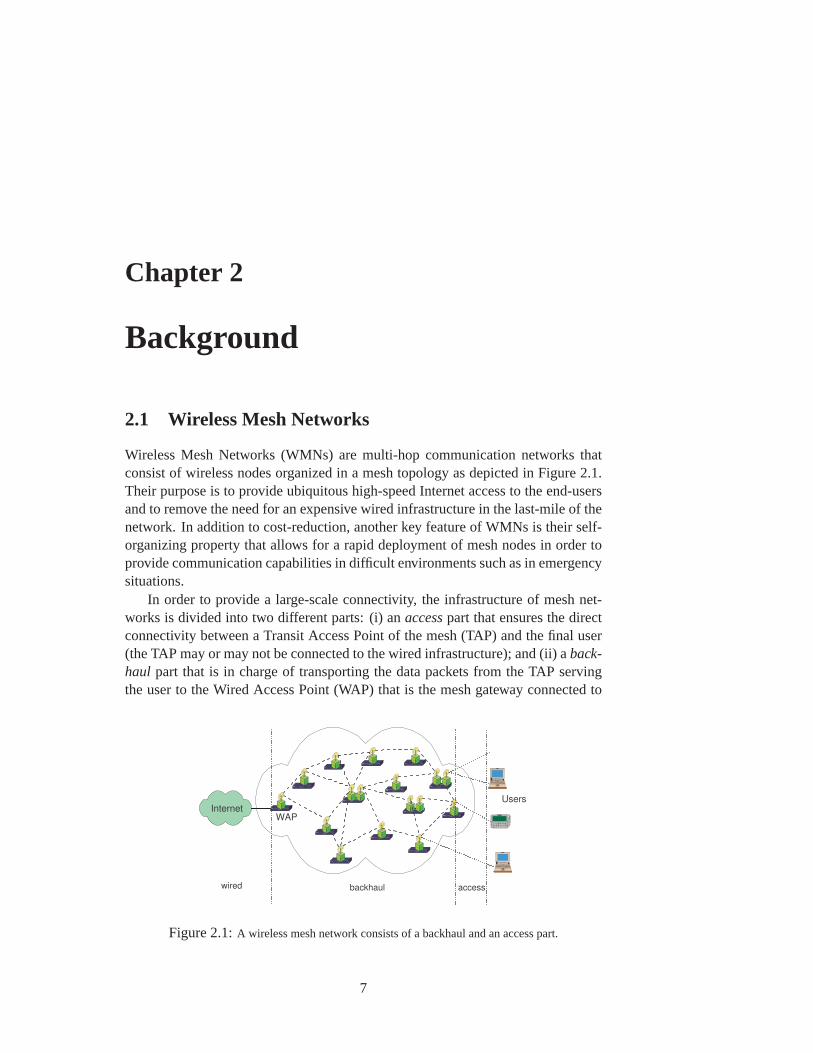
Wireless Mesh Networks (WMNs) are multi-hop communication networks thatconsist of wireless nodes organized in a mesh topology as depicted in Figure 2.1.Their purpose is to provide ubiquitous high-speed Internet access to theend-usersand to remove the need for an expensive wired infrastructure in the last-mileof thenetwork. In addition to cost-reduction, another key feature of WMNs is their self-organizing property that allows for a rapid deployment of mesh nodes in order toprovide communication capabilities in difficult environments such as in emergencysituations.
In order to provide a large-scale connectivity, the infrastructure of mesh net-works is divided into two different parts: (i) anaccesspart that ensures the directconnectivity between a Transit Access Point of the mesh (TAP) and the final user(the TAP may or may not be connected to the wired infrastructure); and (ii) aback-haul part that is in charge of transporting the data packets from the TAP servingthe user to the Wired Access Point (WAP) that is the mesh gateway connectedto
Internet
backhaul
UsersRT 311MODEL
ä
Gateway Router
Gateway Router
RT 311MODEL
PWR TEST LNK/ACT 100 LNK/ACT
INTERNETLOCAL
RIM
RT 311MODEL
ä
Gateway Router
Gateway Router
RT 311MODEL
PWR TEST LNK/ACT 100 LNK/ACT
INTERNETLOCAL
RT 311MODEL
ä
Gateway Router
Gateway Router
RT 311MODEL
PWR TEST LNK/ACT 100 LNK/ACT
INTERNETLOCAL
RT 311MODEL
ä
Gateway Router
Gateway Router
RT 311MODEL
PWR TEST LNK/ACT 100 LNK/ACT
INTERNETLOCAL
RT 311MODEL
ä
Gateway Router
Gateway Router
RT 311MODEL
PWR TEST LNK/ACT 100 LNK/ACT
INTERNETLOCAL
RT 311MODEL
ä
Gateway Router
Gateway Router
RT 311MODEL
PWR TEST LNK/ACT 100 LNK/ACT
INTERNETLOCAL
RT 311MODEL
ä
Gateway Router
Gateway Router
RT 311MODEL
PWR TEST LNK/ACT 100 LNK/ACT
INTERNETLOCAL
RT 311MODEL
ä
Gateway Router
Gateway Router
RT 311MODEL
PWR TEST LNK/ACT 100 LNK/ACT
INTERNETLOCAL
RT 311MODEL
ä
Gateway Router
Gateway Router
RT 311MODEL
PWR TEST LNK/ACT 100 LNK/ACT
INTERNETLOCAL
RT 311MODEL
ä
Gateway Router
Gateway Router
RT 311MODEL
PWR TEST LNK/ACT 100 LNK/ACT
INTERNETLOCAL
RT 311MODEL
ä
Gateway Router
Gateway Router
RT 311MODEL
PWR TEST LNK/ACT 100 LNK/ACT
INTERNETLOCAL
RT 311MODEL
ä
Gateway Router
Gateway Router
RT 311MODEL
PWR TEST LNK/ACT 100 LNK/ACT
INTERNETLOCAL
RT 311MODEL
ä
Gateway Router
Gateway Router
RT 311MODEL
PWR TEST LNK/ACT 100 LNK/ACT
INTERNETLOCAL
RT 311MODEL
ä
Gateway Router
Gateway Router
RT 311MODEL
PWR TEST LNK/ACT 100 LNK/ACT
INTERNETLOCAL
accesswired
WAP
Figure 2.1:A wireless mesh network consists of a backhaul and an access part.
7
8 CHAPTER 2. BACKGROUND
the wired infrastructure. We note that the connectivity problems existing in boththe access and backhaul part can be seen as two separate sub-problems by consid-ering that (i) the access points are equipped with two wireless interfaces dedicatedto either the access or the backhaul, and (ii) each interface is configuredto run inan independent channel. The access part of WMNs will not be the focus of thisthesis, as it is similar to the scheduling problem of single-hop WiFi networks thathas been heavily studied in the literature [Bia00].
Instead, the backhaul part brings multiple new and interesting challenges dueto its multi-hop nature that requires the system to be decentralized and adaptive.Indeed, in order for a self-organizing system to optimally transport data packets ina hop-by-hop manner from a mesh node (TAP) to the mesh gateway (WAP),manytechnical challenges need to be solved such as spectrum management, scheduling,congestion-control, routing and security.
In this thesis, we focus more specifically on the problems of scheduling andcongestion-control. To better understand the nature of these two problems, a use-ful analogy is found in the vehicular traffic problem, where (i) data packets areseen as cars, (ii) single-hop links are seen as streets, and (iii) intermediatenodesare seen as road intersections controlled by a traffic light.The scheduling is then similar to a traffic-light problem:”When should the trafficlight at an intersection turn red or green in order to avoid/minimize collisions andto maximize the number of cars going through?”The challenge in WMNs comesfrom the shared nature of the wireless medium, which implies that two neighboringnodes cannot transmit (i.e., turn green) simultaneously without creating a collision.Therefore, nodes cannot take the scheduling decision independently from each oth-ers, but the lack of central authority (as in traffic-light management) requires thedesign of efficient distributed stochastic scheme to perform the schedulingdecisionat each node.The congestion-control problem takes into account the relation between the dif-ferent links (i.e., streets) of an end-to-end path and it answers the question, ”Howshould the traffic light been controlled at the intersections in order to avoid the cre-ation of a traffic jam in any street of the path?”In WMNs, traffic jams correspondto data packets being queued at intermediate nodes. This is an important problem,because not only does it increase the end-to-end delay of each packet but it canalso lead to packet being dropped (i.e., lost) due to the limited hardware size ofthebuffer at the intermediate nodes. Moreover, in WMNs few or no informationis ex-plicitly available concerning the status of the other links of the path that may varyover time. Thus, there is a need to propose some smart and adaptive schemes thatcan cope with the time-variability of both the links quality, and the traffic demand.
Real deployments of mesh networks already exist in academia [ROO, KZP06],in residential communities [FRE, NAN] and as industrial products [EAR, THE].These deployments use a free standard technology (i.e., IEEE 802.11) that was notdesigned for multi-hop communications: this resulted in some interesting experi-mental findings, such as”with current commodity wireless technology it does not

2.2. THE LAYER MODEL 9
make sense to handle more than three hops”1. In this thesis we do not focus ontop-down approaches resulting in clean-slate design, because we wantto proposesolutions that work on existing deployments with off-the-shelf hardware. Instead,we study analytically the root causes behind the3-hop boundary of IEEE 802.11mesh networks and then we follow a bottom-up approach to propose solutionsthatimprove performance and are backward-compatible with existing designs.
2.2 The Layer Model
The challenges in communication networks are usually tackled by dividing thesystem into different layers, where each layer is responsible for transparently pro-viding some features to the layer above. The first model traditionally proposed isthe Open Systems Interconnection model (OSI model), which divides the network-ing stack into seven independent layers. Most of the current protocolsare based onthe TCP/IP model that we will use hereafter.
Transport
Data Link
Network
Application
Presentation
Session
Physical
Transport
Network
Application
MAC
TCP/IP model OSI model
Figure 2.2:The two layer models used in communication systems and their mapping.
In this model, the four layers are:
• Medium Access Control (MAC) layer: It is responsible for transmitting thedata to the physical medium. To do so, it decides when to transmit a packetto the next-hop and it verifies its successful reception without collision (e.g.,through the use of an acknowledgment scheme). We note that it is not re-sponsible for ensuring that the packet is not dropped at the next-hop after asuccessful reception (e.g., due to buffer overflow).
• Network layer: Based on the end-to-end destination, it is responsible formaking the routing decision and for informing the MAC layer of the iden-tity of the next-hop node. The most commonly used network layer we willconsider hereafter is the Internet Protocol (IP).
1Lunar project: http://cn.cs.unibas.ch/projects/lunar/
10 CHAPTER 2. BACKGROUND
• Transport layer: It is responsible for ensuring the end-to-end connectivitybetween two hosts. The two standard protocols are: (i) the User DatagramProtocol (UDP), which is connectionless (i.e., best-effort) and is commonlyused for voice or video traffic; (ii) the Transmission Control Protocol (TCP),which is connection-oriented and provides reliable in-order packet deliveryto the upper-layer by performing end-to-end congestion control.
• Application layer: It is the highest networking layer responsible for receivingand delivering the data to the final application.
In this work, we propose to tackle both the scheduling and congestion-controlproblem by focusing on the MAC and network layers. Moreover, performing thecongestion control at the transport layer provides good performance inthe wiredInternet, where packet losses are mostly due to buffer overflows and can be seenas a sign of congestion in the network. Wireless multi-hop networks are funda-mentally different, because of the variability of the wireless channel that leads topacket losses and high delays. Indeed, TCP communications running on multi-hopwireless links show relatively poor performance with low throughput [GSK04].
Performing congestion control in a hop-by-hop manner instead of end-to-endhas been shown to have the potential to improve the performance in a wirelessmulti-hop network [YS07]. Therefore, an interesting alternative for the backhaulof wireless mesh networks is to move the congestion-control feature from the trans-port to the network layer. An additional advantage of such a change is that it alsocovers the cases of voice and video traffic that are typical in emergencysituationsand that run over the UDP protocol. For the case of data communication requir-ing to keep the in-order reliable delivery of TCP without congestion-control, newtransport or application protocols can be designed. Therefore, as thein-order re-liable delivery of the transport layer is out-of scope of this thesis, we mostlybaseour study on UDP traffic that requires us to provide congestion control at a lowerlayer.
2.3 The IEEE 802.11 Protocol
The set of standards in the IEEE 802.11 family includes different modulationtech-niques that operate in the 2.4 GHz and 5 GHz frequency bands and that use thesame basic protocol [IEE99]. The first release includes the IEEE 802.11b and theIEEE 802.11a protocols. The IEEE 802.11b protocol runs on the 2.4 GHzband byusing Direct-Sequence Spread Spectrum modulation (DSSS) and it provides datarates up to 11 Mb/s. This protocol divides the frequency into 13 channelsof 22MHz, which are spaced 5 MHz apart, thus making only up to three orthogonalchannels. The IEEE 802.11a protocol runs on the 5 GHz band by using Orthog-onal Frequency-Division Multiplexing (OFDM) and it provides data ratesup to54 Mb/s. After that, new flavors of the IEEE 802.11 protocol appeared;they runon one of these two frequency bands and increase the achievable data rate by using
2.3. THE IEEE 802.11 PROTOCOL 11
Multiple Input Multiple Output (MIMO) techniques. The common point among allthe variations of the IEEE 802.11 family is the main scheduling protocol based onCarrier Sense Multiple Access (CSMA) to decide when to transmit a packet. In thesubsequent section we describe the key components of the IEEE 802.11 protocoland we point to [IEE99] for the technical details.
2.3.1 Description in Single-Hop Environments
The IEEE 802.11 protocol was originally designed for single-hop communications,where the only existing problem is contention (i.e., how to efficiently avoid colli-sions) and not congestion (i.e., how to avoid buffer overflow).In order to solve the contention problem, a nodei that has a packet to send startsthe procedure by uniformly selecting a backoff valueβi in the interval[0; cwi− 1],where the contention windowcwi starts with the minimal valueCWmin (CWmin =25 for 802.11b and24 for 802.11a/g). Then, nodei monitors the medium to assesswhether communications take place or not. For each idle time slot (consisting of20µs for 802.11b and9µs for 802.11a/g), the backoffβi is decremented by one,otherwise it remains frozen if the medium is busy. Eventually, when the backoffreaches zero, nodei sends its packet over the wireless medium and it verifies thesuccessful transmission of the packet to the destination through an acknowledg-ment scheme in which the destination sends an ACK packet after the error-freereception of a data packet.In the case of a successful transmission, the exactly same procedure is repeated forthe next packet in the queue of nodei. However, if an ACK is not received at nodei, the data packet is considered as lost due to contention (i.e., collisions) andthusthe contention windowcwi is doubled before uniformly pickingβi. An unsuccess-ful transmission is repeated at most seven times and at each time,cwi is doubleduntil it reaches the maximal valueCWmax = 210. If the packet is not successfullyreceived after the7th trial, this packet is dropped and the system starts the processagain withcwi = CWmin for the next packet in the queue of nodei. Due to theexponential backoff of IEEE 802.11, this contention-avoidance schemehas beenshown to deliver long-term fairness between the nodes, but not short-term fairness.
Nevertheless, the assumption behind the above process is that all the nodescan correctly detect when the medium is idle or busy (i.e., all nodes are within thesame collision domain) and therefore collisions only occur when at least two nodesrandomly pick the same backoffβ. Even in single-hop communications, this as-sumption can be violated if two clients are in the transmission range of the gatewaybut not in the sensing range of each other (e.g., due to walls). This situation, knownas thehidden-node terminal, leads to a serious performance degradation in CSMAschemes due to repeated collisions between the clients that cannot detect transmis-sions from each other. The cause of this problem is that the channel condition seenat the receiver is not known by the sender, and the solution in single-hopscenariosis to add a collision avoidance scheme. In IEEE 802.11, it is implemented throughthe optional use of Request-To-Send (RTS) and Clear-To-Send (CTS) messages.

12 CHAPTER 2. BACKGROUND
WAP Node1 Node4Node3Node2
transmission/sensing range of Node
Data flow
2
Figure 2.3:Simple4-hop linear scenario leading to problems with IEEE 802.11.
These messages inform all the nodes in the neighborhood of the source and thedestination of the duration of the data exchange. With RTS/CTS, a node startsbysending a RTS message when its backoff expires and it waits to receive a CTS fromthe destination before sending the data packet. In the meanwhile, all the nodes thathear the RTS or CTS set their Network Allocation Vector (NAV), which ensuresthat they remain silent for the entire duration of the transmission. Despite its colli-sion avoidance property, the RTS/CTS mechanism also leads to message overheadand performance losses therefore it is rarely used in practice (i.e., RTS/CTS isturned off by default).
2.3.2 Challenges in Multi-Hop Environments
The IEEE 802.11 protocol was designed for single-hop communications, eventhough it is currently heavily used in multi-hop scenarios such as in mesh net-works. Unfortunately, there are fundamental differences between a single-hop andmulti-hop environment, which make the protocol behave poorly in the latter case.Below, we discuss two features of the protocol that lead to poor performance ina simple linear4-hop scenario as the one depicted in Figure 2.3. This problemtakes the form of network instability where the queue of the first relay builds-upindefinitely.
Exponential Backoff and Collision Avoidance
In [AKT08], we show that the CSMA/CA mechanism as it is implemented in IEEE802.11 leads to poor performance, because nodes may be silent upon thereceptionof an RTS, even though no complete data exchange takes actually place.
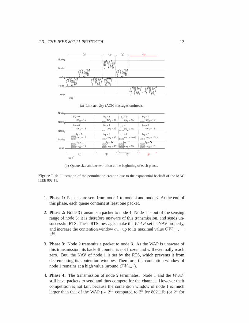
To better understand this problem, we illustrate it through an example thatbuilds upon four phases. Figure 2.4(a) depicts the transmissions as a function ofthe time, whereas Figure 2.4(b) shows the corresponding queues (b1, b2, b3) and thevalues of the contention window (cw0, cw1, cw2, cw3) for the topology depicted inFigure 2.3. We assume that the WAP always has traffic to send, so that its bufferis full (b0 = ∞), and we start with node1 having already4 packets buffered. The4-phase scenario leading to the build-up of node1 is then:
2.3. THE IEEE 802.11 PROTOCOL 13
WAP
Node1
Node2
Node4
Node3
xxxxxxxxxxxxxxxxxxxxxxxxxxxxxxxxxxxxxxxxxxxxxxxxxxxxxxxxxxxxxxxxxxxxxxxxxxxxxxxxxxxxxxxxxxxxxxxxxxxxxxxxxxxxxxxxxxxxxxxxxxxxxxxxxxxxxxxxxxxxxxx
xxxxxxxxxxxxxxxxxxxxxxxxxxxxxxxxxxxxxxxxxxxxxxxxxxxxxxxxxxxxxxxxxxxxxxxxxxxxxxxxxxxxxxxxxxxxxxxxxxxxxxxxxxxxxxxxxxxxxxxxxxxxxxxxxxxxxxxxxxxxxxxxxxxxxxxxxxxxxxxxxxxxxxxxxxxxxxxxxxxxxxxxxxxxxxx
xxxxxxxxxxxxxxxxxxxxxxxxxxxxxxxxxxxxxxxxxxxxxxxx
RT
S
CT
S
DA
TAxxxxxx
xxxxxxxxxxxxxxxxxx
xxxxxxxxxxxxxxxxxx
xx
xx
xxxx
xx
xxxxxxxxxxxxxxxxxxxxxxxxxxxxxxxxxxxx
xxxxxxxxxxxxxxxxxxxxxxxxxxxxxxxxxxxx
RT
S
CT
S
DA
TA
xxxxxxxxxxxxxxxxxx
xxxxxxxxxxxxxxxxxx
xxxx
xxxx
xxxx
xxxx
xxxxxxxxxxxxxxxxxxxxxxxxxxxxxxxxxxxxxxxxxxxxxxxx
xxxxxxxxxxxxxxxxxxxxxxxxxxxxxxxxxxxxxxxxxxxxxxxx
RT
S
CT
S
DA
TAxxxxx
xxxxxxxxxxxxxxx
xxxxxxxxxxxxxxxxxx
xx
xx
xxxx
xxx
xxxxxxxxxxxxxxxxxxxxxxxxxxxxxxxxxxxxxxxxxxxxxxxx
xxxxxxxxxxxxxxxxxxxxxxxxxxxxxxxxxxxxxxxxxxxxxxxx
RT
S
CT
S
DA
TAxxxxxx
xxxxxxxxxxxxxxxxxx
xxxxxxxxxxxxxxxxxxxx
x
xx
xxxx
xxx
xxxxxxxxxxxxxxxxxxxxxxxxxxxxxxxxxxxx
xxxxxxxxxxxxxxxxxxxxxxxxxxxxxxxxxxxx
RT
S
CT
S
DA
TA
xxxxxxxxxxxxxxxxxx
xxxxxxxxxxxxxxxxxx
xxxx
xxxx
xxxx
xxxx
xxxxxxxxxxxxxxxxxxxxxxxxxxxxxxxxxxxxxxxxxxxxxxxx
xxxxxxxxxxxxxxxxxxxxxxxxxxxxxxxxxxxx
RT
S
CT
S
DA
TAxxxxx
xxxxxxxxxxxxxxx
xxxxxxxxxxxxxxxxxx
xx
xx
xxxx
xxx
xxxxxxxxxxxxxxxxxxxxxxxxxxxxxxxxxxxxxxx
xxxxxxxxxxxxxxxxxxxxxxxxxxxxxxxxxxxxxxx
RT
S
CT
S
DA
TA
xxxxxxxxxxxxxxx
xxxxxxxxxxxxxxxxxxxxxxxx
xx
xx
xxxx
xxxx...
xxxxxxxxxxxxxxxx xxxxxxxxxxxxxxxxxxxxxxxxxxxxxxxxxxxxxxxxxxxxxxxxxxxxxxxxxxxxxxxxxxx1 2 3 4
time
RT
S(a) Link activity (ACK messages omitted).
WAP
Node1
Node2
Node4
Node3
xxxxxxxxxxxxxxxxxxxxxxxxxxxxxxxxxxxxxxxxxxxxxxxxxxxxxxxxxxxxxxxxxxxxxxxxxxxxxxxxxxxxxxxxxxxxxxxxxxxxxxxxxxxxxxxxxxxxxxxxxxxxxxxxxxxxxxxxxxxxxxxx
xxxxxxxxxxxxxxxxxxxxxxxxxxxxxxxxxxxxxxxxxxxxxxxxxxxxxxxxxxxxxxxxxxxxxxxxxxxxxxxxxxxxxxxxxxxxxxxxxxxxxxxxxxxxxxxxxxxxxxxxxxxxxxxxxxxxxxxxxxxxxxxx
xxxxxxxxxxxxxxxxxxxxxxxxxxxxxx xxxxxxxxxxxxxxxxxxxxxxxxxxxxxxxxxxxxxxxxxxxxxxxxxxxxxxxxxxxxxxxxxxx
1 2 3 4
time
xxxxxxxxxxxxxxxxxxxxxxxxxxxxxxxxxxxxxxxxxxxxx
xxxxxxxxxxxxxxxxxxxxxxxxxxxxxxxxxxx
xxxxxxxxxxxxxxxxxxxxx
xxxxxxxxxxxxxxxxxxxxx
xxxxxxxxxxxxxx
b0 =
b1 = 2
cw1 = 15
cw0 = 15xxxxxxxxxxxxxxxxxxxxxxxxxxxxxxxxxxxxxxxx
xxxxxxxxxxxxxxxxxxxxxxxx
xxxxxxxxxxxxxxxxxxxxxxxx
xxxxxxxxxxxxxxxx
cw0 = 15xxxxxxxxxxxxxxxxxxxxxxxxxxxxxxxxxxxxxx
xxxxxxxxxxxxxxxxxxxxx
xxxxxxxxxxxxxxxxxxxxxxxx
xxxxxxxxxxxxxxxx
cw0 = 15
xxxxxxxxxxxxxxxxxxxxxxxx
b2 = 0
cw2 = 15
xxxxxxxxxxxxxxxxxxxxxxxx
b3 = 1
cw3 = 15
xxxxxxxxxxxxxxxxxxxxxxxxxxxxxxxxxxxxxxxxxxxxxxxxxxxxxxxxxxxxxxx
xxxxxxxxxxxxxx
b1 = 4
cw1 = 15
b3 = 0
cw3 = 15
b2 = 1
cw2 = 15
xxxxxxxxxxxxxxxxxxxxxxxxxxxxxxxxxxx
xxxxxxxxxxxxxxxxxxxxx
b3 = 0
cw3 = 15
b2 = 1
cw2 = 15
b1 = 2
cw1 = 1023xxxxxxxxxxxxxxxxxxxxxxxxxxxxxxxxxxxxxxxxxxxxxxxx
b1 = 2
cw1 = 1023
xxxxxxxxxxxxxxxxxxxxxxxxxxxxxxxxxxxxxxxx
xxxxxxxxxxxxxxxxxxxxxxxx
xxxxxxxxxxxxxxxxxxxxxxxx
xxxxxxxxxxxxxxxx
cw0 = 15
xxxxxxxxxxxxxxxx
b3 = 1
cw3 = 15
b2 = 0
cw2 = 15
b0 = b0 = b0 =
(b) Queue size andcw evolution at the beginning of each phase.
Figure 2.4: Illustration of the perturbation creation due to the exponential backoff of the MACIEEE 802.11.
1. Phase 1:Packets are sent from node1 to node2 and node3. At the end ofthis phase, each queue contains at least one packet.
2. Phase 2:Node3 transmits a packet to node4. Node1 is out of the sensingrange of node3: it is therefore unaware of this transmission, and sends un-successful RTS. These RTS messages make theWAP set its NAV properly,and increase the contention windowcw1 up to its maximal valueCWmax =210.
3. Phase 3:Node2 transmits a packet to node3. As the WAP is unaware ofthis transmission, its backoff counter is not frozen and will eventually reachzero. But, the NAV of node1 is set by the RTS, which prevents it fromdecrementing its contention window. Therefore, the contention window ofnode1 remains at a high value (aroundCWmax).
4. Phase 4: The transmission of node2 terminates. Node1 and theWAPstill have packets to send and thus compete for the channel. However theircompetition is not fair, because the contention window of node1 is muchlarger than that of the WAP (∼ 210 compared to25 for 802.11b (or24 for

14 CHAPTER 2. BACKGROUND
802.11a) in our example, a ratio factor of32 (or even64)!). This unfairadvantage implies that theWAP will win the competition for the channelmany times in a row. As a result, the queue of node1 builds up.
This example shows that the exponential backoff with RTS/CTS as implemented inIEEE 802.11 exacerbates the instability problem in multi-hop networks. However,we stress that these mechanisms are not the root cause of instability. Indeed, inChapter 3 we analytically prove that the instability problem already occurs in morefundamental schemes such as CSMA.
2.3.3 IEEE 802.11s
In July 2004, a Task Group was created to develop a new amendment to the IEEE802.11 standard (called IEEE 802.11s) in order to address the challenges relativeto the multi-hop environment of mesh networks. The goal of the IEEE 802.11sprotocol is to perform routing at the MAC layer and also to bring security andcongestion control to mesh networks.
In order to deal with congestion control, the task group proposes to use anexplicit congestion notification message that is sent by a node to its neighborsso that they can adapt their sending rate. In Chapter 5, we will show that itispossible to eliminate these explicit notification messages by taking advantage ofthe broadcast nature of the wireless medium.
2.4 Desired Properties of Mesh Networks
Having described the goals, the architecture, and the challenges of IEEE802.11wireless mesh networks, we now clearly state the system properties that arere-quired for the large-scale adoption of WMNs.
• High Throughput: Mesh networks need to be efficient and thus they shouldbe able to deliver an end-to-end throughput that is as close as possible tothetheoretical network capacity. To achieve this, WMNs need to avoid sufferingfrom the typical sources of throughput degradation such as packet collisionsand buffer overflows.
• Low Delays: Another important metric is the end-to-end delay that has tobe maintained as low as possible in order to support real-time services suchas voice traffic and video on demand. To reach this objective, the networkneeds to be stable with small queues at each of the relay nodes.
• Fairness:The two previous criterion focus on the performance within a sin-gle flow. In a real mesh deployment, there are typically multiple flows con-currently present in the network. Therefore it is important that the networkdelivers a certain level of fairness in order to avoid the complete starvationof certain flows.
2.4. DESIRED PROPERTIES OF MESH NETWORKS 15
• Adaptability: Wireless mesh networks have to cope with two sources ofvariability. The first source comes from the variability of the traffic matrixwith the dynamic arrival or departure of new sources in the network. Thesecond is due to the intrinsic variability of the shared wireless medium thatis vulnerable to a large number of environmental changes (such as peoplepassing by, electronic devices turned on and doors being opened/closed).
• Robustness:As already discussed in Chapter 1, the capacity of a wirelessnetwork significantly differs from a wired network, because it is usually un-known and difficult to measure due to the time-variability. Therefore it isimportant that the network automatically adapts and that the performancedoes not degrade (or even collapse) when the sources receive packets at arate above the network capacity.

16 CHAPTER 2. BACKGROUND
Chapter 3
Modeling the Instability of MeshNetworks
3.1 Background
3.1.1 Problem Statement
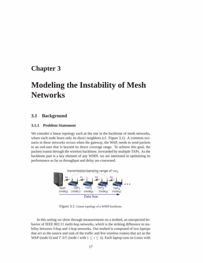
We consider a linear topology such as the one in the backbone of mesh networks,where each node hears only its direct neighbors (cf. Figure 3.1). A common sce-nario in these networks occurs when the gateway, the WAP, needs to sendpacketsto an end-user that is beyond its direct coverage range. To achieve thisgoal, thepackets transit through the wireless backbone, forwarded by multiple TAPs. As thebackbone part is a key element of any WMN, we are interested in optimizing itsperformance as far as throughput and delay are concerned.
WAP TAP1 TAP4TAP3TAP2
transmission/sensing range of
Data flow
TAP2
...(node0) (node4)(node3)(node2)(node1)
z0 z3z2z1
Figure 3.1:Linear topology of a WMN backbone.
In this setting we show through measurements on a testbed, an unexpected be-havior of IEEE 802.11 multi-hop networks, which is the striking difference insta-bility between3-hop and4-hop networks. Our testbed is composed of two laptopsthat act as the source and sink of the traffic and five wireless routers that act as theWAP (node0) andTAPi (nodei with 1 ≤ i ≤ 4). Each laptop runs on Linux with
17

18 CHAPTER 3. MODELING THE INSTABILITY OF MESH NETWORKS
00
10
20
30
40
50
300 600 900 15001200 1800
3-hop
Time
Que
uesi
ze[p
acke
ts]
Node1Node2
00
10
20
30
40
50
300 600 900 1200 1500 1800Time
4-hop
Que
uesi
ze[p
acke
ts]
Node1Node2Node3
Figure 3.2:Experimental results for the queue evolution of each relay node in3-hop and4-hop
topologies. A time slot corresponds to an event when the queue size is recorded, that is every time a
packet arrives at a node.
the softwareIperf1 used to generate saturated UDP traffic with a payload size of1470 bytes. Each laptop is then connected through a wired cable to either theWAPor the last TAP (i.e., node4). The wireless routers are Asus WL-500gP runningthe versionKamikaze 7.07of the OpenWRT firmware2. We change the mini-PCIWiFi cards to Atheros cards in order to benefit from the flexibility of the MadWifidriver [MAD]. This allows the modifications of the driver source code to performboth queue monitoring and the modification of the contention window. We thenset the routers to run in ad-hoc mode on channel13 of IEEE 802.11b at the datarate of 1Mb/s and without RTS/CTS. To avoid interference from neighboring net-works, we perform our measurements in the basement of the BC building at EPFL,where no other wireless networks can be sensed. Finally, we set our topology tomatch our theoretical study: direct neighbors can communicate together, but nodesseparated by two hops or more cannot hear each other.
The major finding is the drastically different stability behavior of3-hop and4-hop topologies, which appears to be counter-intuitive. Figure 3.2 showsthat the3-hop topology is stable, but the4-hop network is unstable. Furthermore, the4-hop instability is due to node1, whose queue length exhibits a transient behavior,i.e., which grows indefinitely until it reaches the hardware limit (50 packets for ourrouters).
In this chapter we seek to better understand the root causes behind this exper-imental stability result. Toward this goal, we introduce an analytical model thatis inspired from the behavior of CSMA/CA protocols (e.g., 802.11-like protocols)with some necessary simplifications for the sake of tractability. We emphasize that,given the mathematical assumptions, our analysis is exact.
1Iperf - The TCP/UDP bandwidth measurement tool: http://dast.nlanr.net/Projects/Iperf/2OpenWRT firmware: http://openwrt.org/
3.1. BACKGROUND 19
3.1.2 Related Work
The unarguable success of the IEEE 802.11 [IEE99] protocol in WiFi communi-cations has lead to the current development of a new draft focusing on multi-hopnetworks such as WMNs, 802.11s [CK, DBvdVH08]. However, until thereleaseof 802.11s, 802.11b/g remains the standard and it is therefore essential tounder-stand its behavior. Towards this goal, previous works [AKT08, NL07, DBvdVH08]present drawbacks of the current protocol in a multi-hop environment. In [GSK08],Garetto et al. present a model to derive the throughput of flows in a multi-hop net-work. Furthermore, Ng et al. identify the existence of an optimal offered loadand propose source-rate limiting at the application layer as a solution [NL07]. Ourapproach differs in the sense that we introduce an analytical model that focuseson queue stability and therefore gives insight into the existence of a maximal fea-sible load. Furthermore our stabilization strategy uses solely the MAC layer andtherefore does not impose any limiting requirements on the client side.
Tackling the congestion problem at the transport layer, e.g. TCP, is studiedin [SGM+08, RJJP08]. Shi et al. focus on inter-flow competition by studying thestarvation occurring when a one-hop flow competes with a two-hop flow andpro-pose a counter-starvation technique that solves the problem. Similarly Rangwalaet al. propose another rate-control protocol that achieves better fairness and effi-ciency than TCP. Our work differs as we focus on the link competition that takesplace within a single flow and study the factors leading to the transition from sta-bility to instability. Thus, rather than relying on the transport layer, we throttlecongestion at the MAC (link) layer (in the OSI model, this functionality of thelink layer is referred to as flow control [GK80]). Analytical and simulation re-sults showing that a hop-by-hop congestion algorithm outperforms an end-to-endversion are presented in [YS07] by Yi et al. Their findings reinforce the need toimplement congestion control at the MAC layer.
In [LE99] Luo et al. study the system stability of random access protocolsinsingle-hop settings. Our work goes further by analyzing the multi-hop scenariowhere the queue states of successive nodes are dependent.
The distributed scheduling problem, which aims at ensuring stability and max-imal throughput, has witnessed growing interest in the research community. Theseminal work of Tassiulas [TE92] introduces a back-pressure algorithm that usesglobal network queue information to derive an optimal routing/scheduling policyand achieve stability and maximal throughput. Several extensions of this workhave been conducted, e.g., Ying et al. reduce the number of queues maintained ateach node to enhance scalability [YST08]. Further work on throughputand fairnessguarantee can be found in [CKLS08], where Chapokar et al. introduce a distributedscheduling strategy that attains a guaranteed ratio of the maximal throughput.Amore complete review of the stability problem in scheduling is presented by Yi etal. in [YPC08], where the tradeoff between complexity, utility and delay is dis-cussed in depth. Finally a scheduling policy based on the queue length is presentedand studied analytically by Gupta et al. in [GLS07]. These works proposecon-
20 CHAPTER 3. MODELING THE INSTABILITY OF MESH NETWORKS
ceptual scheduling solutions that keep the network stable, but depart from IEEE802.11 protocols to various extents, and for which no practical implementationex-ists to date. Our work differs from this previous body of work, as we focus on thestability of existingCSMA protocols, e.g. IEEE 802.11. To the best of our knowl-edge, we are the first to identify the key factors (network size and stealingeffect)that affect the network stability. Furthermore, following our analytical study, wedevelop a practical stabilization strategy and validate experimentally our resultswith off-the-shelf hardware.
3.2 Analytical Model
3.2.1 MAC Layer Description
The first common assumption [CKLS08, ES05, LE99, TE92, YST08] is thatof aslotted discrete-time axis, in other words, each transmission takes one time slotand all the transmissions occurring during a given slot start and finish atthe sametime. We consider a greedy source model, i.e., the WAP (gateway) always hasnew packets ready for transmission. Assuming aK-hop system, the packets flowfrom the WAP toTAPK , via TAP1, TAP2, . . ., TAPK−1. TAPs do not generatepackets of their own. Each TAP is equipped with an infinite buffer.
We assume that the system evolves according to a two-phase mechanism: alinkcompetition phaseand atransmission phase. The link competition phase, whoselength is assumed to be negligible, occurs at the beginning of each slot. Duringthis phase, all the nodes with a non-empty queue compete for the channel and apattern of successful transmissions emerges, referred to astransmission patternin this chapter. Given the current state of queues, the link competition process isassumed to be independent of competitions that happened in previous slots.Thisassumption is similar to the commonly used assumption of exponentially (memo-ryless) distributed backoffs. During this phase, non-empty nodes are sequentiallychosen at random and added to the transmission pattern if and only if they donotinterfere with already selected communications (with the notable exception of thestealing effectdescribed in Section 3.2.3). The final pattern is obtained when nomore nodes can be added without interfering with the others.
The second phase of the model is fairly straightforward as it consists in apply-ing the transmission pattern from the previous phase in order to update the queuestatus of the system. This queue status information is of utmost importance forour analysis because it is the parameter that indicates whether the network remainsstable (no queue explodes) or suffers congestion (one or more queues build up).
3.2.2 Discrete Markov Chain Model
We now formalize the model previously described mathematically. All packets aregenerated by the WAP (node 0), and are forwarded to the last TAP (node K) bysuccessive transmissions via the intermediate nodes (TAPs) 1 toK−1. A time step
3.2. ANALYTICAL MODEL 21
n ∈ N corresponds to the successful transmission of a packet from some node i toits neighbori + 1, or if K is large enough, of a set of packets from different non-interfering nodesi, j, . . . to nodesi + 1, j + 1, . . ., provided these transmissionsoverlap in time (the transmitters and receivers must therefore not interferewitheach other). We assume that node0 always has packets to transmit (infinite queue),and that nodeK consumes immediately the packets, as it is the exit point of thebackbone (its queue is always0). We are interested in the evolution of the queuesizesbi of relaying nodes1 ≤ i ≤ K − 1 over time, and therefore we adopt, as astate variable of the system at timen, the vector
~b(n) = [b1(n) b2(n) . . . bK−1(n)]T ,
with T denoting transposition. We also introduce a set ofK auxiliary binary vari-ableszi, 0 ≤ i ≤ K − 1, representing theith link activity at time slotn: zi(n) = 1if a packet was successfully transmitted from nodei to nodei + 1 during thenth
time slot, andzi(n) = 0 otherwise. Observing that
bi(n+ 1) = bi(n) + zi−1(n)− zi(n),
we can recast the dynamics of the system as
~b(n+ 1) = ~b(n) +A ∗ ~z(n) (3.1)
where
~z(n) = [z0(n) z1(n) z2(n) . . . zK−1(n)]T
A =
1 −1 0 . . . 0
0 1 −1 0...
..... . . . . . .. 0
0 . . . 0 1 −1
.
Finally, the activity of a linkzi depends on the queue sizes of all the nodes, whichwe cast aszi = gi(~b) for some random functiongi(·) of the queue size vector, orin vector form as
~z(n) = g(~b(n)). (3.2)
The specification ofg = [g0, . . . , gK−1]T is the less straightforward part of the
model, as it requires entering in some additional details of the CSMA/CA protocol,which we defer to the next sections. We will first expose it in Section 3.3 foraK = 3 hops network, and then move to the larger networks withK = 4 andK ≥ 5 in the subsequent section, as the specification ofg comes with some levelof complexity asK gets larger. Nevertheless, we can already mention here twosimple constraints thatg must verify:
1. Nodei cannot transmit if its queue is empty, and therefore we havezi =gi(~b) = 0 if bi = 0;
22 CHAPTER 3. MODELING THE INSTABILITY OF MESH NETWORKS
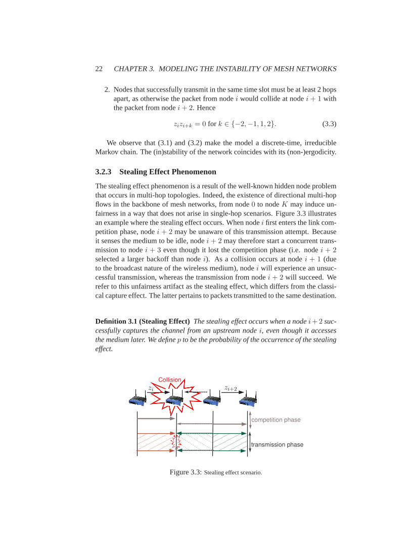
2. Nodes that successfully transmit in the same time slot must be at least 2 hopsapart, as otherwise the packet from nodei would collide at nodei + 1 withthe packet from nodei+ 2. Hence
zizi+k = 0 for k ∈ {−2,−1, 1, 2}. (3.3)
We observe that (3.1) and (3.2) make the model a discrete-time, irreducibleMarkov chain. The (in)stability of the network coincides with its (non-)ergodicity.
3.2.3 Stealing Effect Phenomenon
The stealing effect phenomenon is a result of the well-known hidden nodeproblemthat occurs in multi-hop topologies. Indeed, the existence of directional multi-hopflows in the backbone of mesh networks, from node0 to nodeK may induce un-fairness in a way that does not arise in single-hop scenarios. Figure 3.3illustratesan example where the stealing effect occurs. When nodei first enters the link com-petition phase, nodei + 2 may be unaware of this transmission attempt. Becauseit senses the medium to be idle, nodei + 2 may therefore start a concurrent trans-mission to nodei + 3 even though it lost the competition phase (i.e. nodei + 2selected a larger backoff than nodei). As a collision occurs at nodei + 1 (dueto the broadcast nature of the wireless medium), nodei will experience an unsuc-cessful transmission, whereas the transmission from nodei + 2 will succeed. Werefer to this unfairness artifact as the stealing effect, which differs from the classi-cal capture effect. The latter pertains to packets transmitted to the same destination.
Definition 3.1 (Stealing Effect) The stealing effect occurs when a nodei+2 suc-cessfully captures the channel from an upstream nodei, even though it accessesthe medium later. We definep to be the probability of the occurrence of the stealingeffect.
Collision
competition phase
transmission phase
zi zi+2
Figure 3.3:Stealing effect scenario.
3.3. STABILITY OF3-HOP NETWORKS 23
In IEEE 802.11, the stealing effect corresponds to the event where node i + 2captures the channel, even though it has a larger backoff value than node i. Theprobability of this event occurring depends on the specific protocol implementa-tion. If the optional RTS/CTS handshake is disabled, thenp → 1. If RTS/CTSis enabled, thenp is typically much smaller, but still non-zero because RTS mes-sages may collide [SGM+08]. Indeed, the transmission time of a control message(e.g., the RTS transmission time at the 1Mb/s basic rate is352µs) is non-negligiblecompared to the duration of a backoff slot (20µs).
In our model, the stealing effect is captured by having the functiong(·) in(3.2) depend onp. As revealed by our analysis, a positive and somewhat counter-intuitive consequence of the stealing effect is the promotion of a laminar packetflow, specifically, a smooth propagation of packets. Indeed, by favoring down-stream links over upstream ones, this creates a form of virtual back-pressure thatprevents packets from being pushed too quickly into the network.
3.2.4 Stability Definition
A queue is stable when its occupancy does not tend to increase indefinitely.Moreformally, we adopt the usual definitions of stability (see e.g. Section 2.2 of [BJL08]).
Definition 3.2 (Stability) A queue is stable when its evolution is ergodic (it goesback to zero almost surely in a finite time). A network is stable when the queues ofall forwarding nodes (i.e., all TAPs) are stable.
3.3 Stability of 3-Hop Networks
Let us first analyze the3-hop topology, which remains relatively simple becauseonly one link can be active at a given time slot. Indeed, the only three possibletransmission patterns are
~z ∈ {[1 0 0]T , [0 1 0]T , [0 0 1]T }.
We can now complete the description of the functiong(·), before analyzing theergodicity of the Markov chain.
3.3.1 System Evolution
The role of the stochastic functiong(·) is to map a queue status~b to a transmissionpattern~z with a certain probability.
First, in the case of an idealized CSMA/CA model without the stealing effect(p = 0), all non-empty nodes have exactly the same probability of being scheduled.That is, if only node0 and node1 (or, respectively, node2) have a packet to send,both patterns[1 0 0]T and [0 1 0]T (resp.,[0 0 1]T ) happen with a probability
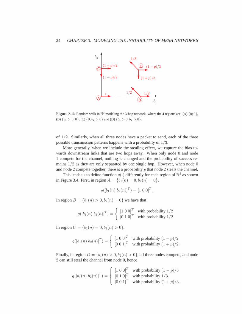
24 CHAPTER 3. MODELING THE INSTABILITY OF MESH NETWORKS
B
CD
Ab1
b2
1/2 1/21
(1− p)/2
(1 + p)/2
1/3
(1− p)/3
(1 + p)/3
Figure 3.4:Random walk inN2 modeling the3-hop network. where the 4 regions are: (A){0; 0},
(B) {b1 > 0; 0}, (C) {0; b2 > 0} and (D){b1 > 0; b2 > 0}.
of 1/2. Similarly, when all three nodes have a packet to send, each of the threepossible transmission patterns happens with a probability of1/3.
More generally, when we include the stealing effect, we capture the bias to-wards downstream links that are two hops away. When only node0 and node1 compete for the channel, nothing is changed and the probability of successre-mains1/2 as they are only separated by one single hop. However, when node0and node2 compete together, there is a probabilityp that node2 steals the channel.
This leads us to define functiong(·) differently for each region ofN2 as shownin Figure 3.4. First, in regionA = {b1(n) = 0, b2(n) = 0},
g([b1(n) b2(n)]T ) = [1 0 0]T .
In regionB = {b1(n) > 0, b2(n) = 0} we have that
g([b1(n) b2(n)]T ) =
{
[1 0 0]T with probability1/2[0 1 0]T with probability1/2.
In regionC = {b1(n) = 0, b2(n) > 0},
g([b1(n) b2(n)]T ) =
{
[1 0 0]T with probability(1− p)/2
[0 0 1]T with probability(1 + p)/2.
Finally, in regionD = {b1(n) > 0, b2(n) > 0}, all three nodes compete, and node2 can still steal the channel from node0, hence
g([b1(n) b2(n)]T ) =
[1 0 0]T with probability(1− p)/3
[0 1 0]T with probability1/3[0 0 1]T with probability(1 + p)/3.

3.3. STABILITY OF3-HOP NETWORKS 25
3.3.2 Stability Analysis
The queue evolution from (3.1) is a random walk inN2, as depicted in Figure 3.4.
Theorem 3.1 shows the stabilizing influence of the stealing effect.
Theorem 3.1 A 3-hop network is unstable for the casep = 0 and it is stable forall 0 < p ≤ 1.
Proof: The instability of the casep = 0 is readily proved with the non-ergodicitytheorem (see Appendix A) using the Lyapunov function
h(b1, b2) = b1, (3.4)
and setting the constantsc = d = 1.
Indeed, it is easy to note that in this case
E
[
h(~b(n+ 1)) | h(~b(n))]
− h(~b(n)) ≥ 0,
is verified for all the three regions of the space satisfyingh(~b(n) > 1 (i.e., theregionsB, C andD).
Next we prove the stability of the cases0 < p ≤ 1 by using Foster’s theorem(see Appendix) with the Lyapunov function
h(b1, b2) = b21 + b22 − b1b2,
the finite setF = {0 ≤ b1, b2 < 5/p} ,
the functionk = 1 and the notations
µb1,b2(n) = E
[
h(~b(n+ 1)) | h(~b(n)) = h(b1, b2)]
ǫb1,b2(n) = µb1,b2(n)− h(b1, b2),
whereǫb1,b2(n) can be interpreted as the drift of the random walk at timen. Thenwe verify Foster’s theorem for all the three regions ofN
2 \ F .After some computations, we find that for RegionB \ F ,
ǫb1,0(n) =1
2(b1 + 1)2 +
1
2((b1 − 1)2 + 1− (b1 − 1))− b21
= 2− b1(n)/2 < 0.
Likewise, for regionC \ F , we get
ǫ0,b2(n) =1 + p
2(b2 − 1)2 +
1− p
2(1 + b22 − b2)− b22
= 1− (3 + p)b2(n)/2 < 0.

26 CHAPTER 3. MODELING THE INSTABILITY OF MESH NETWORKS
0 2 4 6 8 10
x 106
0
5
10
15
20
Time [in slot]
Que
ue s
ize
at n
ode
1
Queue evolution (p=1)
0 2 4 6 8 10
x 106
0
1000
2000
3000
4000
5000
Time [in slot]
Que
ue s
ize
at n
ode
1
Queue evolution (p=0)
0 2 4 6 8 10
x 106
0
20
40
60
80
Time [in slot]
Que
ue s
ize
at n
ode
1
Queue evolution (p=0.1)
0 2 4 6 8 10
x 106
0
100
200
300
400
500
Time [in slot]
Que
ue s
ize
at n
ode
1
Queue evolution (p=0.01)
Figure 3.5:Queue evolution for3-hop with differentp values.
Finally, for regionD \ F , we have
ǫb1,b2(n) =1− p
3((b1 + 1)2 + b22 − (b1 + 1)b2) +
1
3((b1 − 1)2 + (b2 + 1)2 − (b1 − 1)(b2 + 1)) +
1 + p
3(b21 + (b2 − 1)2 − b1(b2 − 1)) +
b1b2 − b21 − b22
=1− p
3(1 + 2b1 − b2) +
1
3(3− 3b1 + 3b2) +
1 + p
3(1 + b1 − 2b2)
= 5/3− p(b1(n) + b2(n))/3 < 0.
Consequently, the two conditions of the theorem are satisfied and stability is proved.�
Finally, we simulate our Markov chain model in MATLAB and in Figure 3.5we present the effect ofp on the queue evolution. We also mention, that our the-oretical results give insight into monitoring the queue of node 1 in order to assessthe stability of the system (i.e., the Lyapunov function of (3.4) only considersb1 toprove instability).
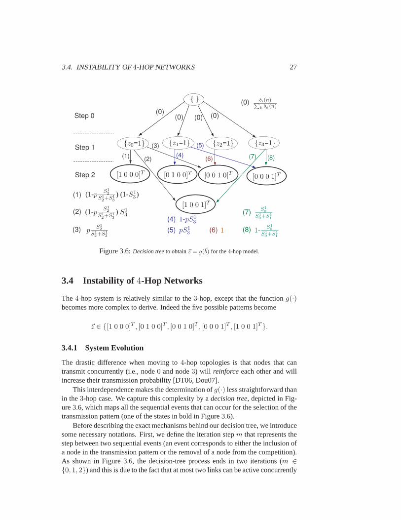
3.4. INSTABILITY OF 4-HOP NETWORKS 27
Step 0
Step 1
Step 2
(2)(1) (8)(7)(6)
(3)
(4)
(5)
(2)
(1)
(8)
(7)
(6)(3)
(4)
(5)
(0)
(0)(0) (0) (0)
(1-p S12
S12+S1
3) (1-S1
3 )
(1-p S12
S12+S1
3) S1
3
pS12
S12+S1
3
1-pS13
pS13 1
S10
S10+S1
1
1- S10
S10+S1
1
δi(n)∑k δk(n)
{z0=1} {z1=1} {z2=1} {z3=1}
{ }
[1 0 0 0]T [0 1 0 0]T [0 0 1 0]T [0 0 0 1]T
[1 0 0 1]T
Figure 3.6:Decision treeto obtain~z = g(~b) for the4-hop model.
3.4 Instability of 4-Hop Networks
The 4-hop system is relatively similar to the3-hop, except that the functiong(·)becomes more complex to derive. Indeed the five possible patterns become
~z ∈ {[1 0 0 0]T , [0 1 0 0]T , [0 0 1 0]T , [0 0 0 1]T , [1 0 0 1]T }.
3.4.1 System Evolution
The drastic difference when moving to4-hop topologies is that nodes that cantransmit concurrently (i.e., node0 and node3) will reinforceeach other and willincrease their transmission probability [DT06, Dou07].
This interdependence makes the determination ofg(·) less straightforward thanin the3-hop case. We capture this complexity by adecision tree, depicted in Fig-ure 3.6, which maps all the sequential events that can occur for the selection of thetransmission pattern (one of the states in bold in Figure 3.6).
Before describing the exact mechanisms behind our decision tree, we introducesome necessary notations. First, we define the iteration stepm that represents thestep between two sequential events (an event corresponds to either the inclusion ofa node in the transmission pattern or the removal of a node from the competition).As shown in Figure 3.6, the decision-tree process ends in two iterations (m ∈{0, 1, 2}) and this is due to the fact that at most two links can be active concurrently
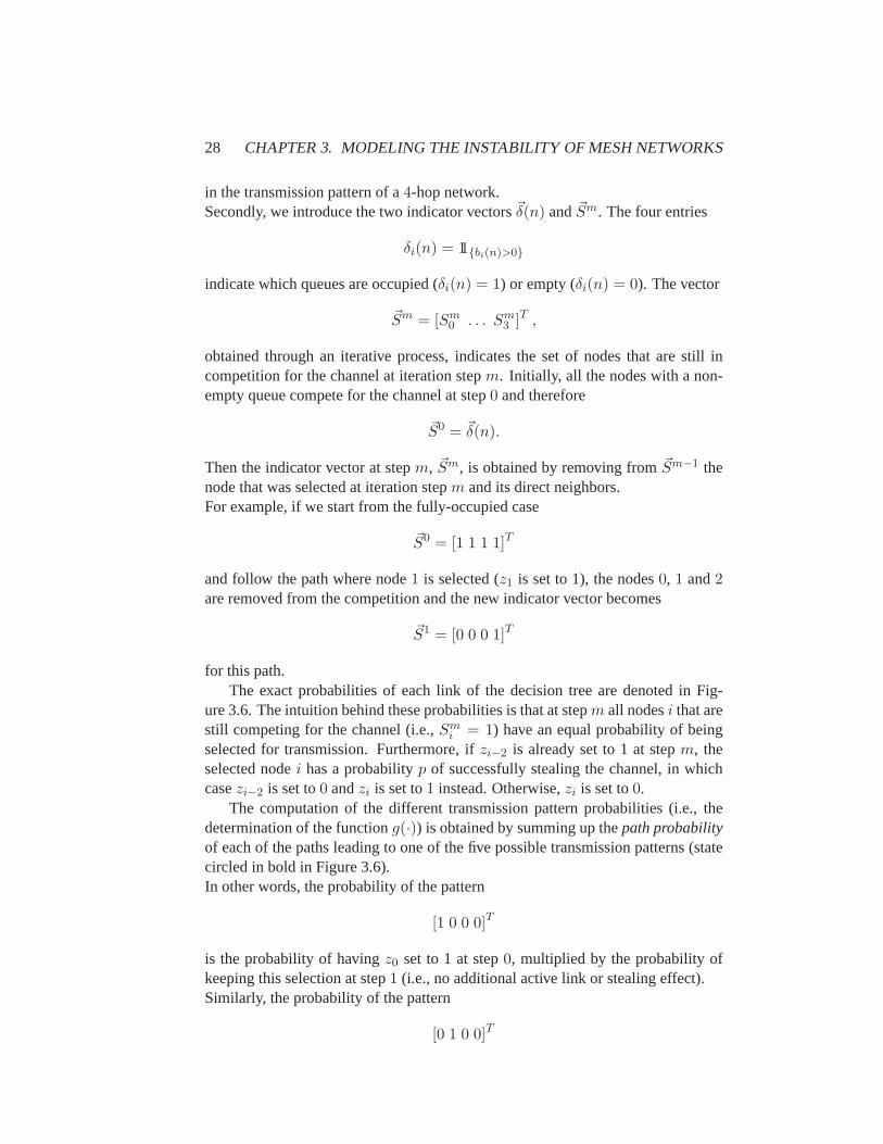
28 CHAPTER 3. MODELING THE INSTABILITY OF MESH NETWORKS
in the transmission pattern of a4-hop network.Secondly, we introduce the two indicator vectors~δ(n) and~Sm. The four entries
δi(n) = 11{bi(n)>0}
indicate which queues are occupied (δi(n) = 1) or empty (δi(n) = 0). The vector
~Sm = [Sm0 . . . Sm
3 ]T ,
obtained through an iterative process, indicates the set of nodes that are still incompetition for the channel at iteration stepm. Initially, all the nodes with a non-empty queue compete for the channel at step0 and therefore
~S0 = ~δ(n).
Then the indicator vector at stepm, ~Sm, is obtained by removing from~Sm−1 thenode that was selected at iteration stepm and its direct neighbors.For example, if we start from the fully-occupied case
~S0 = [1 1 1 1]T
and follow the path where node1 is selected (z1 is set to 1), the nodes0, 1 and2are removed from the competition and the new indicator vector becomes
~S1 = [0 0 0 1]T
for this path.The exact probabilities of each link of the decision tree are denoted in Fig-
ure 3.6. The intuition behind these probabilities is that at stepm all nodesi that arestill competing for the channel (i.e.,Sm
i = 1) have an equal probability of beingselected for transmission. Furthermore, ifzi−2 is already set to 1 at stepm, theselected nodei has a probabilityp of successfully stealing the channel, in whichcasezi−2 is set to0 andzi is set to1 instead. Otherwise,zi is set to0.
The computation of the different transmission pattern probabilities (i.e., thedetermination of the functiong(·)) is obtained by summing up thepath probabilityof each of the paths leading to one of the five possible transmission patterns (statecircled in bold in Figure 3.6).In other words, the probability of the pattern
[1 0 0 0]T
is the probability of havingz0 set to 1 at step0, multiplied by the probability ofkeeping this selection at step1 (i.e., no additional active link or stealing effect).Similarly, the probability of the pattern
[0 1 0 0]T

3.4. INSTABILITY OF 4-HOP NETWORKS 29
is the probability of havingz1 set to 1 at step0, multiplied by the probability ofkeeping this selection at step1.Then, the probability of the pattern
[0 0 1 0]T
is obtained by adding: (i) the probability of havingz2 set to 1 at step0, multipliedby the probability of having this selection maintained at step1 and (ii) the prob-ability of havingz0 set to1 at step0, multiplied by the probability of having thestealing effect at step1.Likewise, the probability of the pattern
[0 0 0 1]T
is obtained by adding: (i) the probability of havingz3 set to 1 at step0, multipliedby the probability of having this selection maintained at step1 and (ii) the prob-ability of havingz1 set to1 at step0, multiplied by the probability of having thestealing effect at step1.Finally, the probability of the pattern
[1 0 0 1]T
is obtained by adding: (i) the probability of havingz0 set to1 at step0, multipliedby the probability of havingz3 set to1 at step1 and (ii) the probability of havingz3 set to1 at step0 multiplied by the probability of havingz0 set to1 at step1.
As in Figure 3.4, Figure 3.7 summarizes the probabilities of the transmissionpatterns (i.e.,g(·)) for each of the8 regions ofN3:
A = {0, 0, 0}
B = {b1(n) > 0, 0, 0}
C = {0, b2(n) > 0, 0}
D = {b1(n) > 0, b2(n) > 0, 0}
E = {0, 0, b3(n) > 0}
F = {b1(n) > 0, 0, b3(n) > 0}
G = {0, b2(n) > 0, b3(n) > 0}
H = {b1(n) > 0, b2(n) > 0, b3(n) > 0}.
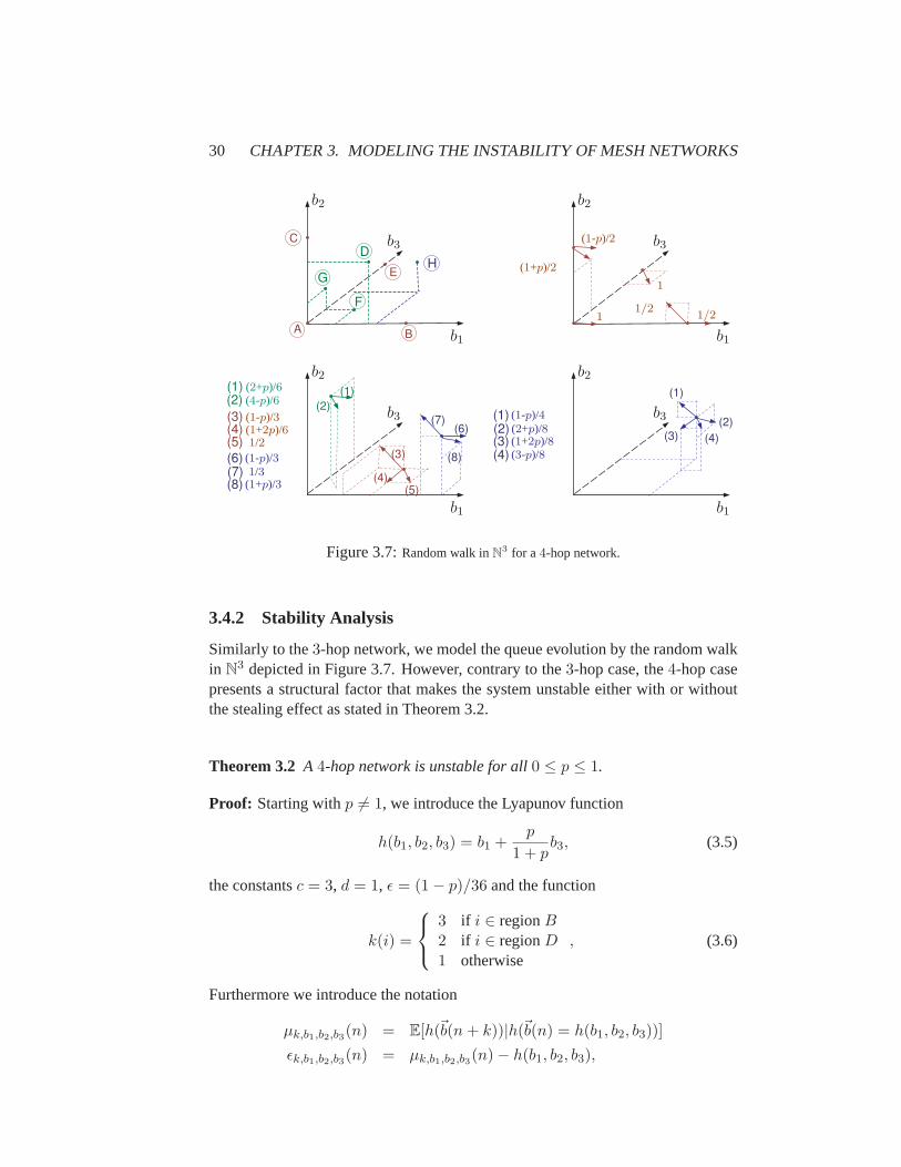
30 CHAPTER 3. MODELING THE INSTABILITY OF MESH NETWORKS
DH
B
G
F
E
C
A b1
b2
b3
b1
b2
b3
1
1
1/21/2
(1+p)/2
(1-p)/2
(1)(2)(1)
(4)(3)
(5)
(6)(7)(8)
(4)
(3)
(5)
(6)(7)
(8)
(2)
b1
b2
b3
(2+p)/6(4-p)/6
(1-p)/3(1+2p)/61/2
(1-p)/31/3
(1+p)/3
(4)
(1)
(2)(3)
(1)(2)(3)(4)
b1
b2
b3(1-p)/4(2+p)/8(1+2p)/8(3-p)/8
Figure 3.7:Random walk inN3 for a4-hop network.
3.4.2 Stability Analysis
Similarly to the3-hop network, we model the queue evolution by the random walkin N
3 depicted in Figure 3.7. However, contrary to the3-hop case, the4-hop casepresents a structural factor that makes the system unstable either with or withoutthe stealing effect as stated in Theorem 3.2.
Theorem 3.2 A 4-hop network is unstable for all0 ≤ p ≤ 1.
Proof: Starting withp 6= 1, we introduce the Lyapunov function
h(b1, b2, b3) = b1 +p
1 + pb3, (3.5)
the constantsc = 3, d = 1, ǫ = (1− p)/36 and the function
k(i) =
3 if i ∈ regionB2 if i ∈ regionD1 otherwise
, (3.6)
Furthermore we introduce the notation
µk,b1,b2,b3(n) = E[h(~b(n+ k))|h(~b(n) = h(b1, b2, b3))]
ǫk,b1,b2,b3(n) = µk,b1,b2,b3(n)− h(b1, b2, b3),
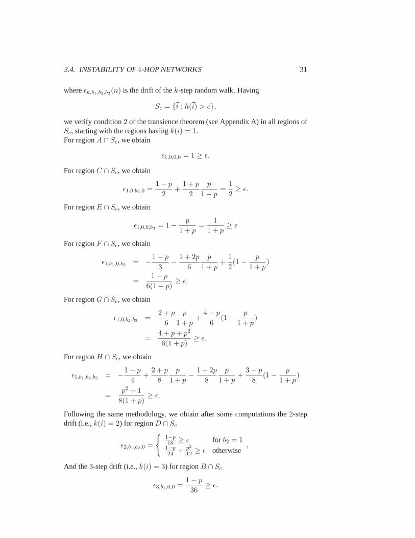
3.4. INSTABILITY OF 4-HOP NETWORKS 31
whereǫk,b1,b2,b3(n) is the drift of thek-step random walk. Having
Sc = {~i : h(~i) > c},
we verify condition2 of the transience theorem (see Appendix A) in all regions ofSc, starting with the regions havingk(i) = 1.For regionA ∩ Sc, we obtain
ǫ1,0,0,0 = 1 ≥ ǫ.
For regionC ∩ Sc, we obtain
ǫ1,0,b2,0 =1− p
2+
1 + p
2
p
1 + p=
1
2≥ ǫ.
For regionE ∩ Sc, we obtain
ǫ1,0,0,b3 = 1−p
1 + p=
1
1 + p≥ ǫ
For regionF ∩ Sc, we obtain
ǫ1,b1,0,b3 = −1− p
3−
1 + 2p
6
p
1 + p+
1
2(1−
p
1 + p)
=1− p
6(1 + p)≥ ǫ.
For regionG ∩ Sc, we obtain
ǫ1,0,b2,b3 =2 + p
6
p
1 + p+
4− p
6(1−
p
1 + p)
=4 + p+ p2
6(1 + p)≥ ǫ.
For regionH ∩ Sc, we obtain
ǫ1,b1,b2,b3 = −1− p
4+
2 + p
8
p
1 + p−
1 + 2p
8
p
1 + p+
3− p
8(1−
p
1 + p)
=p2 + 1
8(1 + p)≥ ǫ.
Following the same methodology, we obtain after some computations the2-stepdrift (i.e., k(i) = 2) for regionD ∩ Sc
ǫ2,b1,b2,0 =
{
1−p18 ≥ ǫ for b2 = 11−p24 + p2
12 ≥ ǫ otherwise,
And the3-step drift (i.e.,k(i) = 3) for regionB ∩ Sc
ǫ3,b1,0,0 =1− p
36≥ ǫ.
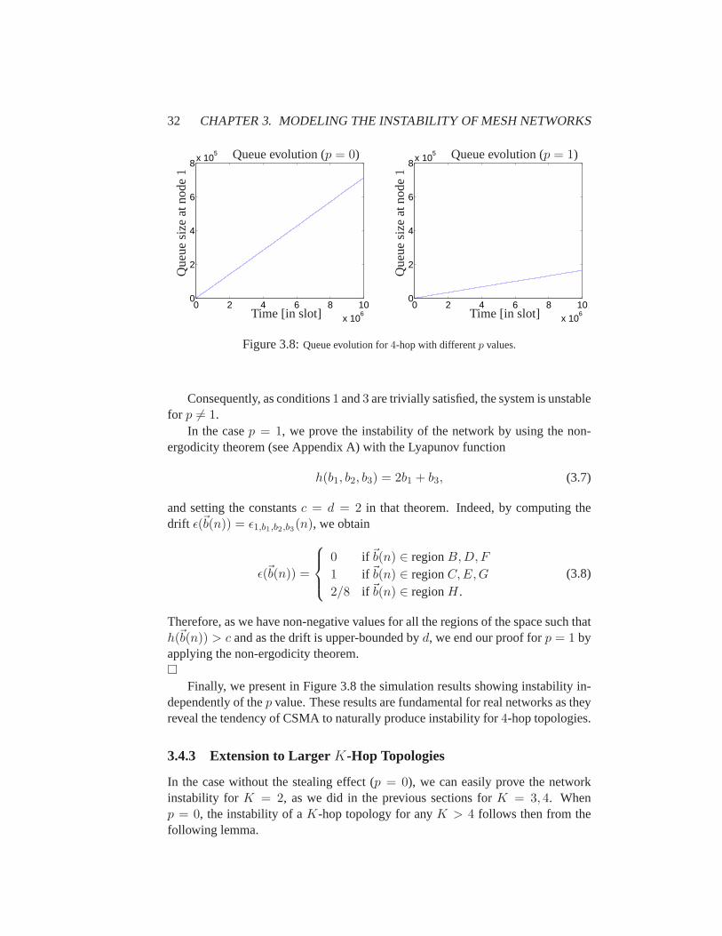
32 CHAPTER 3. MODELING THE INSTABILITY OF MESH NETWORKS
0 2 4 6 8 10x 10
6
0
2
4
6
8x 10⁵ Queue evolution (p = 0)
Que
uesi
zeat
node1
Time [in slot]0 2 4 6 8 10
x 106
0
2
4
6
8x 10⁵ Queue evolution (p = 1)
Que
uesi
zeat
node1
Time [in slot]
Figure 3.8:Queue evolution for4-hop with differentp values.
Consequently, as conditions1 and3 are trivially satisfied, the system is unstablefor p 6= 1.
In the casep = 1, we prove the instability of the network by using the non-ergodicity theorem (see Appendix A) with the Lyapunov function
h(b1, b2, b3) = 2b1 + b3, (3.7)
and setting the constantsc = d = 2 in that theorem. Indeed, by computing thedrift ǫ(~b(n)) = ǫ1,b1,b2,b3(n), we obtain
ǫ(~b(n)) =
0 if ~b(n) ∈ regionB,D, F
1 if ~b(n) ∈ regionC,E,G
2/8 if ~b(n) ∈ regionH.
(3.8)
Therefore, as we have non-negative values for all the regions of thespace such thath(~b(n)) > c and as the drift is upper-bounded byd, we end our proof forp = 1 byapplying the non-ergodicity theorem.�
Finally, we present in Figure 3.8 the simulation results showing instability in-dependently of thep value. These results are fundamental for real networks as theyreveal the tendency of CSMA to naturally produce instability for4-hop topologies.
3.4.3 Extension to LargerK-Hop Topologies
In the case without the stealing effect (p = 0), we can easily prove the networkinstability for K = 2, as we did in the previous sections forK = 3, 4. Whenp = 0, the instability of aK-hop topology for anyK > 4 follows then from thefollowing lemma.
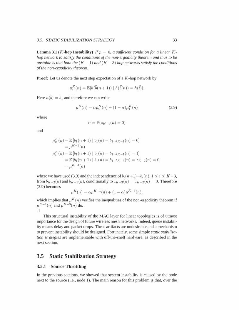
3.5. STATIC STABILIZATION STRATEGY 33
Lemma 3.1 (K-hop Instability) If p = 0, a sufficient condition for a linearK-hop network to satisfy the conditions of the non-ergodicity theorem and thus tobeunstable is that both the(K − 1) and(K − 3) hop networks satisfy the conditionsof the non-ergodicity theorem.
Proof: Let us denote the next step expectation of aK-hop network by
µKi (n) = E[h(~b(n+ 1)) | h(~b(n)) = h(~i)].
Hereh(~b) = b1 and therefore we can write
µK(n) = αµK0 (n) + (1− α)µK
1 (n) (3.9)
whereα = P(zK−1(n) = 0)
and
µK0 (n) = E [b1(n+ 1) | b1(n) = b1, zK−1(n) = 0]
= µK−1(n)
µK1 (n) = E [b1(n+ 1) | b1(n) = b1, zK−1(n) = 1]
= E [b1(n+ 1) | b1(n) = b1, zK−3(n) = zK−2(n) = 0]
= µK−3(n)
where we have used (3.3) and the independence ofbi(n+1)−bi(n), 1 ≤ i ≤ K−3,from bK−2(n) andbK−1(n), conditionally tozK−3(n) = zK−2(n) = 0. Therefore(3.9) becomes
µK(n) = αµK−1(n) + (1− α)µK−3(n),
which implies thatµK(n) verifies the inequalities of the non-ergodicity theorem ifµK−1(n) andµK−3(n) do.�
This structural instability of the MAC layer for linear topologies is of utmostimportance for the design of future wireless mesh networks. Indeed, queue instabil-ity means delay and packet drops. These artifacts are undesirable and amechanismto prevent instability should be designed. Fortunately, some simplestatic stabiliza-tion strategiesare implementable with off-the-shelf hardware, as described in thenext section.
3.5 Static Stabilization Strategy
3.5.1 Source Throttling
In the previous sections, we showed that system instability is caused by the nodenext to the source (i.e., node1). The main reason for this problem is that, over the
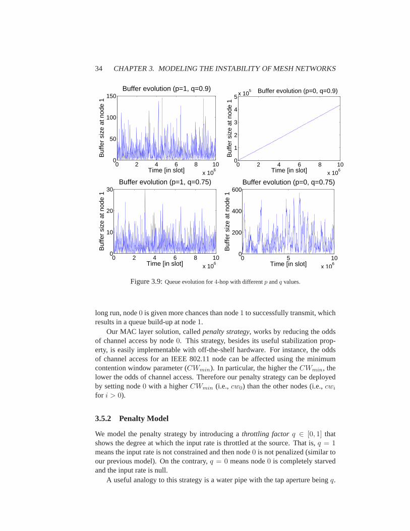
34 CHAPTER 3. MODELING THE INSTABILITY OF MESH NETWORKS
0 2 4 6 8 10x 10
6
0
50
100
150
Time [in slot]
Buf
fer
size
at n
ode
1
Buffer evolution (p=1, q=0.9)
0 2 4 6 8 10x 10
6
0
1
2
3
4
5x 10⁵
Time [in slot]
Buf
fer
size
at n
ode
1
Buffer evolution (p=0, q=0.9)
0 2 4 6 8 10x 10
6
0
10
20
30
Time [in slot]
Buf
fer
size
at n
ode
1
Buffer evolution (p=1, q=0.75)
0 5 10x 10
6
0
200
400
600
Time [in slot]
Buf
fer
size
at n
ode
1
Buffer evolution (p=0, q=0.75)
Figure 3.9:Queue evolution for4-hop with differentp andq values.
long run, node0 is given more chances than node1 to successfully transmit, whichresults in a queue build-up at node1.
Our MAC layer solution, calledpenalty strategy, works by reducing the oddsof channel access by node0. This strategy, besides its useful stabilization prop-erty, is easily implementable with off-the-shelf hardware. For instance, the oddsof channel access for an IEEE 802.11 node can be affected using theminimumcontention window parameter (CWmin). In particular, the higher theCWmin, thelower the odds of channel access. Therefore our penalty strategy can be deployedby setting node0 with a higherCWmin (i.e., cw0) than the other nodes (i.e.,cwi
for i > 0).
3.5.2 Penalty Model
We model the penalty strategy by introducing athrottling factor q ∈ [0, 1] thatshows the degree at which the input rate is throttled at the source. That is,q = 1means the input rate is not constrained and then node0 is not penalized (similar toour previous model). On the contrary,q = 0 means node0 is completely starvedand the input rate is null.
A useful analogy to this strategy is a water pipe with the tap aperture beingq.
3.5. STATIC STABILIZATION STRATEGY 35
The higher the value ofq, the higher the inflow into the network, but also the morelikely the flow will be turbulent. Mapping this back to our system, we deduce thatthere exists a throttling factor thresholdq∗ below which the system is stable.
The impact of the throttling factor is captured in our analytical model by choos-ing node0 with probability
qSm0
qSm0 +
∑
j>0 Smj
,
whereas nodei 6= 0 is selected with probability
Smi
qSm0 +
∑
j>0 Smj
.
For instance, consider aK-hop network where at a given time slot only nodes0 and 1 have packets to transmit: then node 0 wins with probability
P(z0) = q/(1 + q)
and node 1 wins with complementary probability
P(z1) = 1/(1 + q).
3.5.3 Theoretical Analysis
Next we analyze3-hop and4-hop networks, after implementing the penalizationstrategy.
Beginning with the previously unstable3-hop case (p = 0), we prove the stabi-lization effect of the throttling factor and the existence of the thresholdq∗ = 1 byapplying a similar methodology than in Section 3.3.2. That is, using the function
h(b1, b2) = b21 + b22,
and the finite set
F =
{
0 ≤ b1 <3 + q
2(1− q)
}
⋂
{
0 ≤ b2 <1 + q
2
}
,
we verify Foster’s theorem (see Appendix A) and therefore prove thestability ofthe3-hop case for allq < 1.
Next, we consider4-hop topologies. We observe that the stealing effect has animportant impact on stability. Indeed, as depicted on Figure 3.9, the thresholdq∗ ishighly dependent on the stealing effect probabilityp. The higherp, the higherq∗.
We derive theoretical bounds onq∗ as follows. First, we obtain a lower-boundthrough a stability argument. The proof is obtained by a generalized versionofFoster’s theorem (Theorem 2.2.2, [FMM95]) that usesk-step expectation insteadof 1-step expectation. We apply it with the Lyapunov function
h = b1 + b2 + b3,
36 CHAPTER 3. MODELING THE INSTABILITY OF MESH NETWORKS
takingk = 18.The upper-bound is similarly obtained by the non-ergodicity theorem (see Ap-pendix A) with the function
h = b1 +p
1 + pb3
and the parameterk = 15.Following this procedure forp = 0, we obtain
0.37 < q∗ ≤ 0.884.
Similarly, whenp = 1, we find
0.76 < q∗ ≤ 0.964.
It should be noticed that the bounds onq∗ could be made tighter by either inves-tigating different Lyapunov functions or by increasing the valuek (i.e., increasingthe number of steps of thek-steps expectation at the expense of higher computa-tional cost).Nevertheless, the current bounds already validate some results of Figure 3.9. Forinstance,q = 0.75 < 0.76 is stable forp = 1 andq = 0.9 > 0.884 is unstable forp = 0.
3.5.4 Experimental Analysis
We test our stabilization strategy on our experimental testbed described in Sec-tion 3.1. We implement the factorq in our testbed by setting a different value ofCWmin at the WAP (i.e.,cw0) than at the other nodes (i.e.,cwi>0). Thus, to imple-mentq = 1/2, we usecw0 = 26 andcwi>0 = 25. Note that our hardware forcedus to set the contention window as a power of2. The results of Figure 3.10 confirmexperimentally the efficiency of the throttling factor in stabilizing the network. In-deed, a value ofq = 1/2 suffices to change the network behavior from unstable tostable.
Table 3.1 presents mean throughput statistics for different network sizesandvalues ofq. The results are obtained by running experiments for400 s and measur-ing throughput over non-overlapping 5 s intervals. Each entry in the tablethus rep-resents an average of 80 samples. Corresponding standard deviationsare also pro-vided. We make the following observations. First, there is a significant throughputgap between3-hop and4-hop networks, which can be attributed to the distributednature of IEEE 802.11 that does not always make the best spatial reuseof the chan-nel. Second, for the case of4-hop networks, the mean throughput decreases withq,but only whenq becomes very small (i.e.,q = 1/16 or smaller). Up to that point,the overhead caused by using a larger contention window for the WAP is not toosignificant.

3.6. SIMULATIONS ON MULTI-FLOW TOPOLOGIES 37
00
10
20
30
40
50
300 600 900 1200 1500 1800Time
4-hop withq = 1/2
Que
uesi
ze[p
acke
ts]
Node1Node2Node3
00
10
20
30
40
50
300 600 900 1200 1500 1800
4-hop withq = 1/4
Time
Que
uesi
ze[p
acke
ts]
Node1Node2Node3
Figure 3.10:Experimental results for the queue evolution for the4-hop topologies with different
throttling factorsq (we recallq = 1 is unstable).
Mean throughput Standard deviation
3-hop withq = 1 240.5 kb/s 15.8
4-hop withq = 1 146.0 kb/s 16.74-hop withq = 1/2 157.5 kb/s 16.34-hop withq = 1/4 141.5 kb/s 14.54-hop withq = 1/8 143.3 kb/s 17.44-hop withq = 1/16 108.7 kb/s 11.84-hop withq = 1/32 96.9 kb/s 11.14-hop withq = 1/64 81.8 kb/s 13.4
Table 3.1:Mean throughput and standard deviation for networks of different sizes and for different
throttling factorsq.
3.6 Simulations on Multi-Flow Topologies
Up to this point, we have focused on single flow linear topologies as they are thebuilding blocks of more general mesh topologies. However, to show that thesta-bility problem also arises in more complex topologies, in this section we presentthe simulation results obtained with the ns-2 simulator.
We analyze the two multi-flows topologies depicted in Figure 3.11, where sce-nario 1 sees two concurrent flows and scenario2 sees three. Furthermore, weset the simulator to use the standard parameters of IEEE 802.11 ad-hoc networks(RTS/CTS disabled, Tx range:250 m, Cs range:550 m) and let the simulationsrun for respectively1100 s and1600 s.
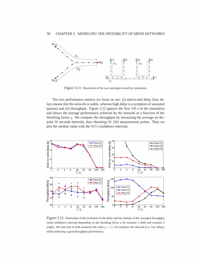
38 CHAPTER 3. MODELING THE INSTABILITY OF MESH NETWORKS
F1
F2
N0
N12
N11
F2 F3
N11N0
N12
F1
N24N23 N35
Figure 3.11:Illustration of the two topologies tested by simulation.
The two performance metrics we focus on are: (i) end-to-end delay (low de-lays means that the network is stable, whereas high delay is a symptom of saturatedqueues) and (ii) throughput. Figure 3.12 ignores the first100 s of the simulationand shows the average performance achieved by the network as a function of thethrottling factorq. We compute the throughput by measuring the average on dis-joint 50 seconds intervals, thus obtaining20 (30) measurement points. Then weplot the median value with the95%-confidence intervals.
1 2 4 8 16 32 64 128 2560
2
4
6
End
−to
−en
d de
lay
[s]
Flow F1Flow F2
1/q2 8 32 1284 16 64 2561
0
10
20
30
40
End
−to
−en
d de
lay
[s]
Flow F1Flow F2Flow F3
1/q
1 2 4 8 16 32 64 128 25665
70
75
80
85
Thr
ough
put [
Kb/
s]
Flow F1Flow F2
1/q1 2 4 8 16 32 64 128 256
0
50
100
150
Thr
ough
put [
Kb/
s]
Flow F1Flow F2Flow F3
1/q
Figure 3.12:Illustration of the evolution of the delay and the median of the averaged throughput
(with confidence interval) depending on the throttling factorq for scenario1 (left) and scenario2
(right). We note that in both scenarios the valueq = 1/128 stabilizes the network (i.e. low delay),
while achieving a good throughput performance.

3.7. INSTABILITY PROBLEM AT HIGHER RATES 39
We note that, for both scenarios, the standard IEEE 802.11 protocol (i.e.q = 1)performs poorly as expected, with high variance in throughput and high end-to-enddelays. Furthermore, using an appropriate throttling factor that is larger than forthe single-flow case (hereq = 1/128), performances are significantly improvedby achieving both negligible delays and higher global throughput due to a lowerpacket loss rate (as no buffer overflow in stable regime).
3.7 Instability Problem at Higher Rates
Our analytical model allows us to explain why a stable3-hop network becomesunstable when a4th hop is added (see Figure 3.2). Nevertheless, the results fromFigure 3.2 are obtained with a fixed data rate of1 Mb/s, a buffer size limit of50packets, and a small-scale testbed where the routers are used without theirexternalantennas (better control on the experimental environment). In order to validateour results on a different setting, we modify the MadWifi driver to unlock thebuffer size limit and to allow for the modification of its value at run time through asimple command (see Appendix B for details). We then set the buffer limit to100packets and repeat the experiment from Figure 3.2 on the real-scale deployment ofFigure 3.13, for different data rate settings.
66 m
0 1
2
3
4
l0
l1
l2
l3
Figure 3.13:Illustration of the deployment used in Section 3.7.
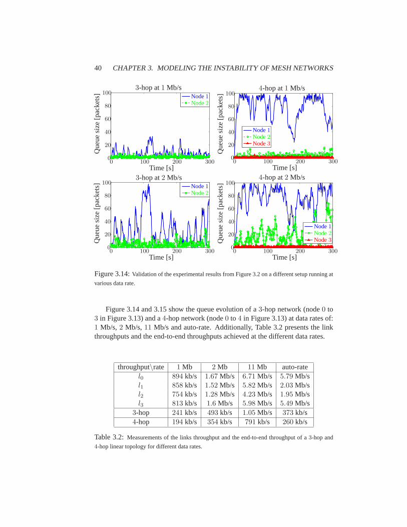
40 CHAPTER 3. MODELING THE INSTABILITY OF MESH NETWORKS
Node1Node2
00
20
40
60
80
100
100 200 300Time [s]
Que
uesi
ze[p
acke
ts] 3-hop at1 Mb/s
Node1Node2Node3
00
20
40
60
80
100
100 200 300Time [s]
Que
uesi
ze[p
acke
ts] 4-hop at1 Mb/s
Node1Node2
00
20
40
60
80
100
100 200 300Time [s]
Que
uesi
ze[p
acke
ts] 3-hop at2 Mb/s
Node1Node2Node3
00
20
40
60
80
100
100 200 300Time [s]
Que
uesi
ze[p
acke
ts] 4-hop at2 Mb/s
Figure 3.14:Validation of the experimental results from Figure 3.2 on a different setup running at
various data rate.
Figure 3.14 and 3.15 show the queue evolution of a3-hop network (node0 to3 in Figure 3.13) and a4-hop network (node0 to 4 in Figure 3.13) at data rates of:1 Mb/s, 2 Mb/s, 11 Mb/s and auto-rate. Additionally, Table 3.2 presents the linkthroughputs and the end-to-end throughputs achieved at the differentdata rates.
throughput\rate 1 Mb 2 Mb 11 Mb auto-ratel0 894 kb/s 1.67 Mb/s 6.71 Mb/s 5.79 Mb/sl1 858 kb/s 1.52 Mb/s 5.82 Mb/s 2.03 Mb/sl2 754 kb/s 1.28 Mb/s 4.23 Mb/s 1.95 Mb/sl3 813 kb/s 1.6 Mb/s 5.98 Mb/s 5.49 Mb/s
3-hop 241 kb/s 493 kb/s 1.05 Mb/s 373 kb/s4-hop 194 kb/s 354 kb/s 791 kb/s 260 kb/s
Table 3.2:Measurements of the links throughput and the end-to-end throughput of a 3-hop and
4-hop linear topology for different data rates.
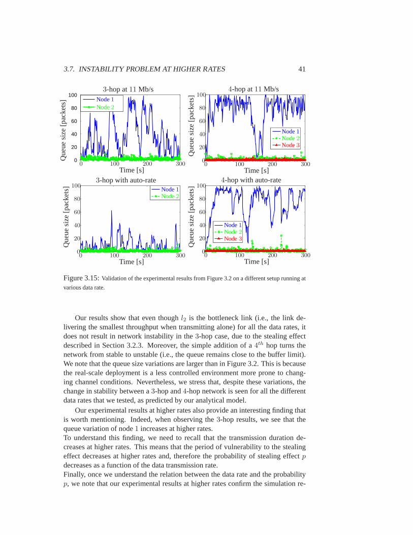
3.7. INSTABILITY PROBLEM AT HIGHER RATES 41
0
20
40
60
80
100
Node1Node2
0 100 200 300Time [s]
Que
uesi
ze[p
acke
ts] 3-hop at11 Mb/s
Node1Node2Node3
00
20
40
60
80
100
100 200 300Time [s]
Que
uesi
ze[p
acke
ts] 4-hop at11 Mb/s
Node1Node2
00
20
40
60
80
100
100 200 300Time [s]
Que
uesi
ze[p
acke
ts] 3-hop with auto-rate
Node1Node2Node3
00
20
40
60
80
100
100 200 300Time [s]
Que
uesi
ze[p
acke
ts] 4-hop with auto-rate
Figure 3.15:Validation of the experimental results from Figure 3.2 on a different setup running at
various data rate.
Our results show that even thoughl2 is the bottleneck link (i.e., the link de-livering the smallest throughput when transmitting alone) for all the data rates, itdoes not result in network instability in the3-hop case, due to the stealing effectdescribed in Section 3.2.3. Moreover, the simple addition of a4th hop turns thenetwork from stable to unstable (i.e., the queue remains close to the buffer limit).We note that the queue size variations are larger than in Figure 3.2. This is becausethe real-scale deployment is a less controlled environment more prone to chang-ing channel conditions. Nevertheless, we stress that, despite these variations, thechange in stability between a3-hop and4-hop network is seen for all the differentdata rates that we tested, as predicted by our analytical model.
Our experimental results at higher rates also provide an interesting finding thatis worth mentioning. Indeed, when observing the3-hop results, we see that thequeue variation of node1 increases at higher rates.To understand this finding, we need to recall that the transmission duration de-creases at higher rates. This means that the period of vulnerability to the stealingeffect decreases at higher rates and, therefore the probability of stealing effectpdecreases as a function of the data transmission rate.Finally, once we understand the relation between the data rate and the probabilityp, we note that our experimental results at higher rates confirm the simulation re-
42 CHAPTER 3. MODELING THE INSTABILITY OF MESH NETWORKS
sults of our analytical model presented in Figure 3.5. In other words, we see thatthe higher the rate (i.e., the smallerp), the closer the queue evolution gets to a nullrecurrent system.
3.8 Concluding Remarks
In this chapter, we addressed the problem of network stability in CSMA-based lin-ear wireless mesh networks and we provided three main contributions. First,weidentified two key factors impacting the stability: the network size and an artifactthat we call the stealing effect. Second, we proved analytically and showed experi-mentally that3-hop networks are stable when we account for the stealing effect, but4-hop networks (and presumably larger topologies) are not. Third, we devised andproved the effectiveness of a simple static stabilization strategy that throttles thesource at the MAC layer, preventing packets from being injected too quickly intothe network. We note that this strategy penalizes only the source when othernodesalso have packets to transmit. This desirable property allows to ensure both stabil-ity and high throughput. Our analysis and experiments have shown that selecting avalueCWmin four to eight times larger at the source than at the relay nodes (i.e.,q = 1/4 or q = 1/8) in the4-hop case effectively achieves these goals. We alsoshowed that multi-flow networks can also be stabilized by using higher valuesofq. As the optimal parameterq is topology-dependent, in the next chapters we willpresent some techniques to automatically adapt the throttling factorq according tothe network environment.
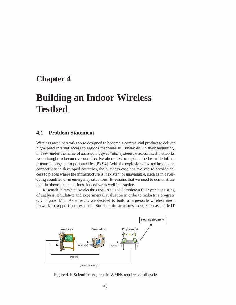
Chapter 4
Building an Indoor WirelessTestbed
4.1 Problem Statement
Wireless mesh networks were designed to become a commercial product to deliverhigh-speed Internet access to regions that were still unserved. In their beginning,in 1994 under the name ofmassive array cellular systems, wireless mesh networkswere thought to become a cost-effective alternative to replace the last-mile infras-tructure in large metropolitan cities [Pie94]. With the explosion of wired broadbandconnectivity in developed countries, the business case has evolved to provide ac-cess to places where the infrastructure is inexistent or unavailable, suchas in devel-oping countries or in emergency situations. It remains that we need to demonstratethat the theoretical solutions, indeed work well in practice.
Research in mesh networks thus requires us to complete a full cycle consistingof analysis, simulation and experimental evaluation in order to make true progress(cf. Figure 4.1). As a result, we decided to build a large-scale wireless meshnetwork to support our research. Similar infrastructures exist, such asthe MIT
Analysis Simulation Experiment
Real deployment
(models) (code)
(measurements)
(results)
Figure 4.1: Scientific progress in WMNs requires a full cycle
43

44 CHAPTER 4. BUILDING AN INDOOR WIRELESS TESTBED
roofnet [ROO] or the Magnets [KZP06] (currently renamed to BOWL1) testbeds.Nevertheless, as we did not have easy day-to-day access to these testbeds and noneexisted at EPFL, we decided to build from scratch our own multi-hop testbed oncampus. During this deployment, we faced multiple challenges and design ques-tions. In this chapter, we share some of the experiences and lessons we learned inthis process.
4.2 Choice of Hardware and Software
4.2.1 Requirements and Challenges
The first step when deploying our indoor mesh network was to set the require-ments for our testbed. In our case, we were interested in matching the followingconstraints.
• Adaptability: Even though our main interest lies in the scheduling problemof IEEE 802.11 mesh networks, we were interested in building a more gen-eral platform that would enable practical investigations of a wide range ofresearch scenarios such as routing, user tracking, mobility, etc.
• Programmability: Due to the research-orientation of our deployment, wechose our hardware and software in order to provide adaptability even ifitis at the cost of a small drop in relative performance. The first effect of thisrequirement appears in our choice of the firmware (openWRT2) and of thedriver (MadWifi3) that are both open-source and thus enable us to modifythe source code in order to meet our research needs.
• Large-scale:Having already performed small-scale experiments (e.g., in thebasement of our school building), we were interested in providing a platformthat is closer to a real deployment. Toward this goal, we designed our testbedto cover six buildings on our campus with different node densities betweenthe buildings.
• Price constraints: Finally, the last constraint we needed to meet was a bud-get constraint that forced us to evaluate different alternatives, in order to findthe hardware that provides the best tradeoff between the different require-ments. We also stress that due to budget reasons, we did not consider theuseof Software Defined Radio (SDR) in our architecture, even though it wastheoption offering the highest level of programmability.
1Berlin Open Wireless Lab (BOWL): http://bowl.net.t-labs.tu-berlin.de/2OpenWRT firmware: http://openwrt.org/3MadWifi driver: http://madwifi-project.org/
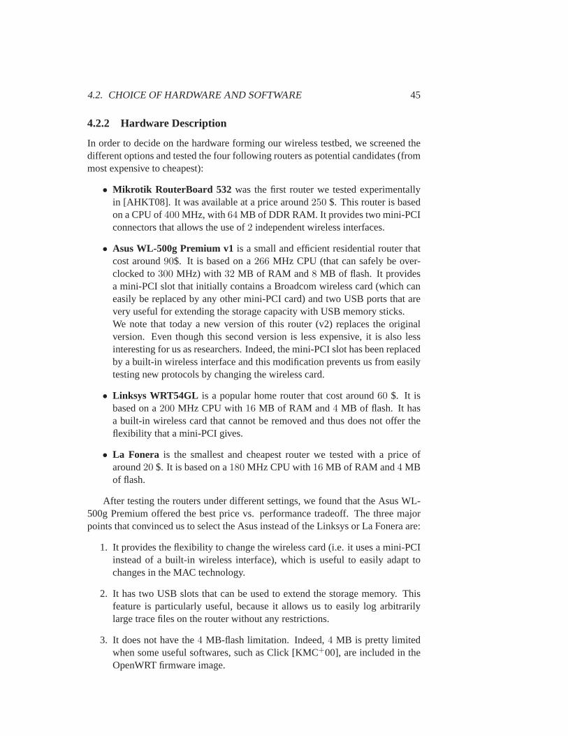
4.2. CHOICE OF HARDWARE AND SOFTWARE 45
4.2.2 Hardware Description
In order to decide on the hardware forming our wireless testbed, we screened thedifferent options and tested the four following routers as potential candidates (frommost expensive to cheapest):
• Mikrotik RouterBoard 532 was the first router we tested experimentallyin [AHKT08]. It was available at a price around250 $. This router is basedon a CPU of400 MHz, with 64 MB of DDR RAM. It provides two mini-PCIconnectors that allows the use of2 independent wireless interfaces.
• Asus WL-500g Premium v1is a small and efficient residential router thatcost around90$. It is based on a266 MHz CPU (that can safely be over-clocked to300 MHz) with 32 MB of RAM and 8 MB of flash. It providesa mini-PCI slot that initially contains a Broadcom wireless card (which caneasily be replaced by any other mini-PCI card) and two USB ports that arevery useful for extending the storage capacity with USB memory sticks.We note that today a new version of this router (v2) replaces the originalversion. Even though this second version is less expensive, it is also lessinteresting for us as researchers. Indeed, the mini-PCI slot has been replacedby a built-in wireless interface and this modification prevents us from easilytesting new protocols by changing the wireless card.
• Linksys WRT54GL is a popular home router that cost around60 $. It isbased on a200 MHz CPU with16 MB of RAM and 4 MB of flash. It hasa built-in wireless card that cannot be removed and thus does not offer theflexibility that a mini-PCI gives.
• La Fonera is the smallest and cheapest router we tested with a price ofaround20 $. It is based on a180 MHz CPU with16 MB of RAM and4 MBof flash.
After testing the routers under different settings, we found that the AsusWL-500g Premium offered the best price vs. performance tradeoff. The three majorpoints that convinced us to select the Asus instead of the Linksys or La Fonera are:
1. It provides the flexibility to change the wireless card (i.e. it uses a mini-PCIinstead of a built-in wireless interface), which is useful to easily adapt tochanges in the MAC technology.
2. It has two USB slots that can be used to extend the storage memory. Thisfeature is particularly useful, because it allows us to easily log arbitrarilylarge trace files on the router without any restrictions.
3. It does not have the4 MB-flash limitation. Indeed,4 MB is pretty limitedwhen some useful softwares, such as Click [KMC+00], are included in theOpenWRT firmware image.
46 CHAPTER 4. BUILDING AN INDOOR WIRELESS TESTBED
(a) (b)
Figure 4.2:The Asus WL-500g Premium that we used in our testbed and where (i) we changed the
WiFi mini-PCI card to an Atheros-based one, and (ii) we designed a technique to power our router
through a battery, which enabled us to support mobile scenarios.
When purchasing our hardware in 2007, we chose the Asus over the Routerboardfor two main reasons. First, the USB capabilities were a useful feature providedonly by the Asus. Second, the small CPU gain of the Routerboard did not justifythe price difference, which was an important factor as we were planning tobuyaround60 routers (i.e., around10, 000 $ difference in the total price). We notethat nowadays, at the end of 2010, an interesting option that we are consideringfor upgrading our testbed are the Alix boards from PC Engines, which have theadvantage of (i) running over an x86 architecture instead of mipsel, and (ii) havingspace for two WiFi interfaces and three antennas (that can for example be used toperform MIMO in IEEE 802.11n).
The Asus routers were provided with a power supply and a standard Broad-com mini-PCI WiFi card. These settings are good for a standard home user, butwe needed to operate two modifications/enhancements in order to support there-search scenario we had in mind (i.e., modifying/monitoring the MAC parametersand supporting mobile scenarios).
• Allow modification/monitoring of MAC parameters: In order to use theopen-source MadWifi driver, we needed to change the mini-PCI card to anAtheros-based one as depicted in Figure 4.2.a. We used the NMP-8602Atheros card that runs on IEEE 802.11a/b/g.
• Enable mobility: In order to eliminate the requirement to plug our routerto the electrical grid (which prevents mobility), we equipped some of ourdevices with6 V batteries as shown in Figure 4.2.b. To be able to meet thehigh amperage requirement to support the wireless interface of our router,
4.2. CHOICE OF HARDWARE AND SOFTWARE 47
we used A 506/10 batteries. Moreover, as the Asus routers work on an inputvoltage of4.5 V, we added two inductances to the cabling connecting thebattery to the router.
In addition to these modifications, we also equipped each router with a2 GB mem-ory stick that is automatically mounted during the boot-up of the router. After morethan one year of constant use, we note that the power supply is the main source offailure of our routers. Indeed, we experienced almost no problems with the routerhardware itself, but we had to replace around10 power supplies that broke down.
4.2.3 OpenWRT Firmware
OpenWRT is a free open-source and Linux-based firmware. We decided to flashour routers with this distribution, because of the facility with which we can (i)install existing program and (ii) deploy our own C code. In Appendix B, weprovidea detailed explanation of the methodology that needs to be followed in order to (i)build an image that is ready to be flashed on the routers, (ii) cross-compile our ownprogram to run on the mipsel architecture of the Asus, and (iii) flash the newimageto the routers and make the first boot-up configuration procedure.
A particularly interesting software to install in the OpenWRT image is theClick modular router [KMC+00]: it allows us to completely control the process-ing/routing of a packet since it arrives to the router until it leaves it.
4.2.4 MadWiFi Driver
MadWifi is an interesting, but challenging wireless driver. On the one hand, itsadvantage comes from its open-source code that leaves room for easymodificationand enhancement of the protocol. On the other hand, it suffers from one of thetypical drawbacks of open-source software, as opposed to industrial products. Forexample, we noted that some of the supposedly working commands were onlypartially implemented (or even not implemented at all).
One of the key advantages that convinced us to adopt MadWifi is that it pro-vides an easy access to multiple MAC parameters of IEEE 802.11, such as theCWmin, CWmax, RTS mode on/off, etc.Nevertheless, we needed to modify ourselves the source code in order toachievethree objectives:
1. We unlocked the modification, via theiwpriv command, of the MAC layerparameters for Best Effort traffic (BE), the standard type of traffic inthenetwork.
2. We enabled the use of multiple MAC queues (up to4 or 8) as it is pro-posed in the IEEE 802.11e standard to achieve Quality of Service. Moreover,the possibility of using different queues is very useful in congestion-controlschemes as it allows us to use different class of service depending on thenature of the next-hop.

48 CHAPTER 4. BUILDING AN INDOOR WIRELESS TESTBED
3. We coded three new functions to thewlanconfigcommand in order to accessthe instantaneous queue occupancy and to access and modify the maximalMAC buffer length (usually locked to50 packets).
As the technical details behind each modification are rather complex, we de-fer their description to Appendix B. Furthermore, we stress that nowadays newopen-source drivers such as ath5k4 and ath9k5 have been launched as follow-upsof MadWifi in order to support the new generations of the IEEE 802.11 family,such as IEEE 802.11n.
4.3 Testbed Deployment
Once we finished with flashing and configuring our60 Asus routers, we had toplan our deployment to be able to cover as many scenarios as possible. We initiallyplanned our deployment for a flexible design in which the routers would be rapidlydeployed and collected back directly after a round of measurements (or atthe endof the day). But, our initial measurements appeared to suffer the same problemsas the ones reported in [PYC06] and we had to reconsider our design. Indeed,we found that simple displacements of a mesh node by as little as a fraction of acentimeters leads to significant changes in the connectivity, from high SNRsto ba-sically no connection at all. This issue was a real limitation for the reproducibilityof the results as it is impossible to guarantee the exact same positioning of a routerbetween two rounds of deployment.
Therefore, we finally decided to have a mostly fixed mesh network testbed with41 routers installed and we kept the others as mobile devices that can rapidly bedeployed for flexibility if needed. For the safety of the hardware, we deployedmost of the routers within private offices. Concerning the routers that needed to bedeployed in public spaces, we modified them to add a locking system in order toattach them to the fixed infrastructure.
4.3.1 Topology
The map of the final topology that we are currently using in our indoor testbed is de-picted in Figure 4.3. We use41 wireless routers that we spread among the6 build-ings of the I&C Faculty. We designed our deployment to form a fully-connectednetwork, with a different node density among different buildings. Among the41routers,37 are connected to the wired infrastructure by using thewpa supplicantsoftware for authentication with the IT infrastructure of the department. The4 re-maining nodes could not be directly connected to the wired infrastructure due totheir location in the inter-building corridors that do not contain any wired connec-tivity plug.
4ath5k driver: http://linuxwireless.org/en/users/Drivers/ath5k5ath9k driver: http://linuxwireless.org/en/users/Drivers/ath9k
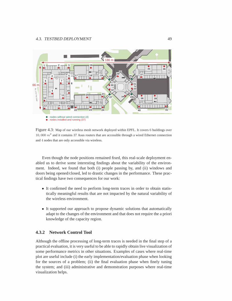
4.3. TESTBED DEPLOYMENT 49
66 m
186 m
: nodes without wired connection (4): nodes installed and running (37)
1 2 3
4 5
6 78
9 10
1112
13 14 15
16
17 18 19
20 21
22 23 24
25 26
27 28
31
32 33
34
36
37
35
38
29
39
30
40 41
Figure 4.3:Map of our wireless mesh network deployed within EPFL. It covers6 buildings over
10, 000 m2 and it contains37 Asus routers that are accessible through a wired Ethernet connection
and4 nodes that are only accessible via wireless.
Even though the node positions remained fixed, this real-scale deployment en-abled us to derive some interesting findings about the variability of the environ-ment. Indeed, we found that both (i) people passing by, and (ii) windows anddoors being opened/closed, led to drastic changes in the performance. These prac-tical findings have two consequences for our work:
• It confirmed the need to perform long-term traces in order to obtain statis-tically meaningful results that are not impacted by the natural variability ofthe wireless environment.
• It supported our approach to propose dynamic solutions that automaticallyadapt to the changes of the environment and that does not require the a prioriknowledge of the capacity region.
4.3.2 Network Control Tool
Although the offline processing of long-term traces is needed in the final step of apractical evaluation, it is very useful to be able to rapidly obtain live visualization ofsome performance metrics in other situations. Examples of cases where real-timeplot are useful include (i) the early implementation/evaluation phase when lookingfor the sources of a problem; (ii) the final evaluation phase when finely tuningthe system; and (iii) administrative and demonstration purposes where real-timevisualization helps.

50 CHAPTER 4. BUILDING AN INDOOR WIRELESS TESTBED
After some investigation, we could not find a software that matches our re-quirements of: (i) allowing the visualization of statistics such as the link through-put and the MAC queue occupancy (obtained after hacking the driver as describedin Appendix B); (ii) allowing to control (i.e., launch commands) in all or part ofthe network from a central server; and (iii) being open-source and allowing sim-ple modification of the source code for the addition of new visualization modulesdepending on the research needs.
Therefore, we developed our own program, calledNet-Controller, that can cre-ate nice dynamic plots representing data collected on-the-fly from the network andthat allows us to send arbitrary commands to any set of nodes. We mention thatsome tools, such as Jigsaw [CBB+06], have been proposed in prior work to allowfor the creation of a packet-level trace by merging the data obtained from multiplesniffers. Net-Controller significantly differs from Jigsaw-like tools in three ways:
• it is both very user-friendly with a graphical interface and easily expandableto monitor arbitrary metrics of interest in the network;
• it does not require dedicated monitoring nodes in the network and thus it isalso able to display internal data that cannot be sniffed on the air, such asthequeue occupancy or the variation in contention window;
• it is not only a monitoring tool. Indeed, Net-Controller allows to modify theparameters of any node in the network, directly from the graphical interface.Moreover, it also enables us to generate traffic from any set of nodesin thenetwork to any other node with only a few mouse clicks (see video6).
Design Description of Net-Controller
We designed Net-Controller to work as two separated sub-programs that commu-nicate together through a network socket (see Figure 4.4).
• The server part runs on a computer (desktop, laptop, or any other devicewith a display). It consists of a simple graphical interface that allows for dy-namic plots to be generated, for the commands to be launched on the nodes,and for traffic to be started (or stopped). Requests are sent periodically tothe nodes in order to retrieve the data to plot. The commands are launchedthroughssh . This program is written in Python and is multi-platform. Itsimply needs to know the IP addresses of the routers to interact with them.
• The client part runs on the wireless routers. Its role is to answer the requestssent by the server with the appropriate values. These values can be instanta-neously obtained at any time (e.g., a queue occupancy), or aggregated (e.g.,the number of bytes received since the last request, in order to compute athroughput). The current version of this module is implemented in C and
6Net-Controller - network management & visualization: http://icawww1.epfl.ch/NetController/
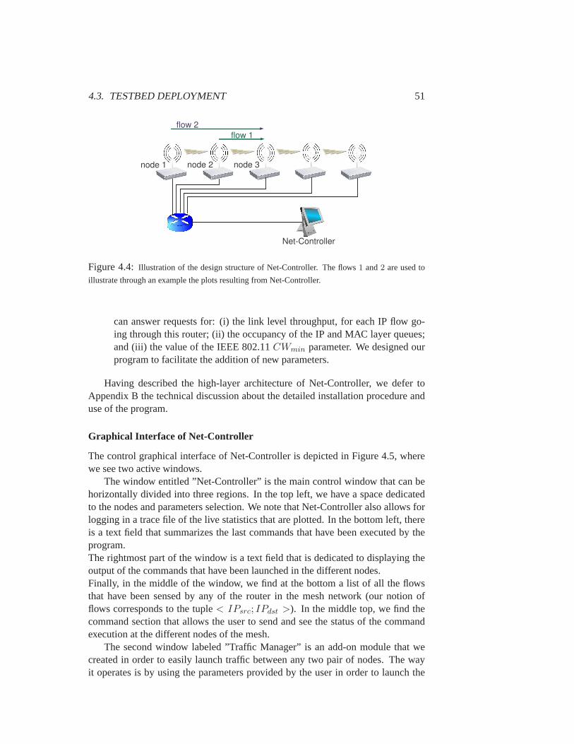
4.3. TESTBED DEPLOYMENT 51
Net-Controller
node 1
flow 1
node 2 node 3
flow 2
Figure 4.4: Illustration of the design structure of Net-Controller. The flows1 and2 are used to
illustrate through an example the plots resulting from Net-Controller.
can answer requests for: (i) the link level throughput, for each IP flowgo-ing through this router; (ii) the occupancy of the IP and MAC layer queues;and (iii) the value of the IEEE 802.11CWmin parameter. We designed ourprogram to facilitate the addition of new parameters.
Having described the high-layer architecture of Net-Controller, we defer toAppendix B the technical discussion about the detailed installation procedure anduse of the program.
Graphical Interface of Net-Controller
The control graphical interface of Net-Controller is depicted in Figure 4.5, wherewe see two active windows.
The window entitled ”Net-Controller” is the main control window that can behorizontally divided into three regions. In the top left, we have a space dedicatedto the nodes and parameters selection. We note that Net-Controller also allowsforlogging in a trace file of the live statistics that are plotted. In the bottom left, thereis a text field that summarizes the last commands that have been executed by theprogram.The rightmost part of the window is a text field that is dedicated to displaying theoutput of the commands that have been launched in the different nodes.Finally, in the middle of the window, we find at the bottom a list of all the flowsthat have been sensed by any of the router in the mesh network (our notionofflows corresponds to the tuple< IPsrc; IPdst >). In the middle top, we find thecommand section that allows the user to send and see the status of the commandexecution at the different nodes of the mesh.
The second window labeled ”Traffic Manager” is an add-on module that wecreated in order to easily launch traffic between any two pair of nodes. The wayit operates is by using the parameters provided by the user in order to launch the
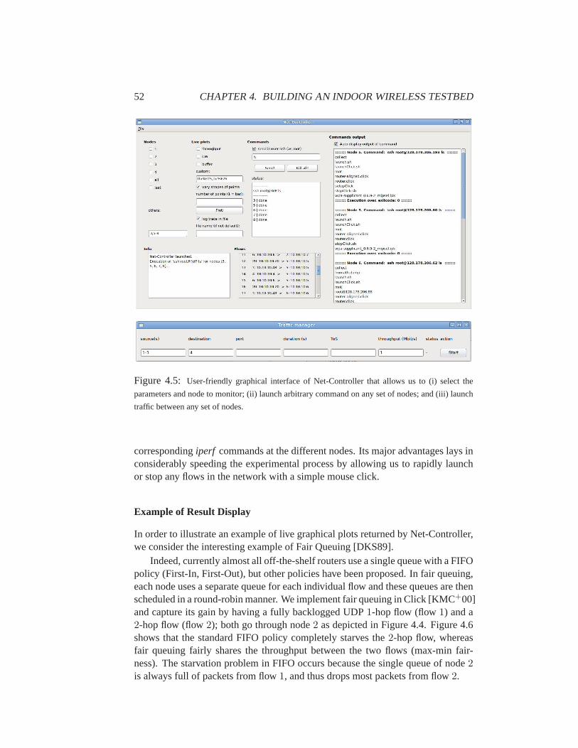
52 CHAPTER 4. BUILDING AN INDOOR WIRELESS TESTBED
Figure 4.5: User-friendly graphical interface of Net-Controller that allows us to (i) select the
parameters and node to monitor; (ii) launch arbitrary command on any set of nodes; and (iii) launch
traffic between any set of nodes.
correspondingiperf commands at the different nodes. Its major advantages lays inconsiderably speeding the experimental process by allowing us to rapidly launchor stop any flows in the network with a simple mouse click.
Example of Result Display
In order to illustrate an example of live graphical plots returned by Net-Controller,we consider the interesting example of Fair Queuing [DKS89].
Indeed, currently almost all off-the-shelf routers use a single queue with a FIFOpolicy (First-In, First-Out), but other policies have been proposed. Infair queuing,each node uses a separate queue for each individual flow and these queues are thenscheduled in a round-robin manner. We implement fair queuing in Click [KMC+00]and capture its gain by having a fully backlogged UDP1-hop flow (flow1) and a2-hop flow (flow2); both go through node2 as depicted in Figure 4.4. Figure 4.6shows that the standard FIFO policy completely starves the2-hop flow, whereasfair queuing fairly shares the throughput between the two flows (max-min fair-ness). The starvation problem in FIFO occurs because the single queueof node2is always full of packets from flow1, and thus drops most packets from flow2.
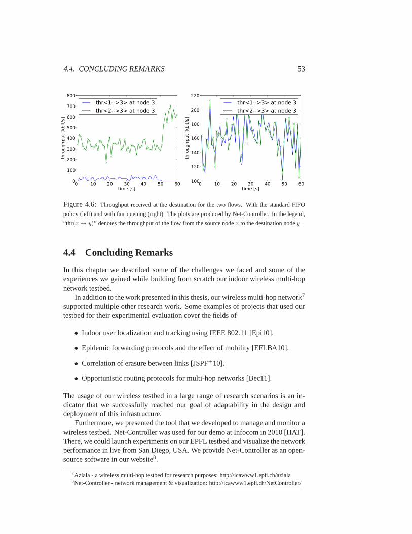
4.4. CONCLUDING REMARKS 53
0 10 20 30 40 50 60time [s]
0
100
200
300
400
500
600
700
800
thro
ughp
ut [k
bit/s
]
thr<1-->3> at node 3thr<2-->3> at node 3
0 10 20 30 40 50 60time [s]
100
120
140
160
180
200
220
thro
ughp
ut [k
bit/s
]
thr<1-->3> at node 3thr<2-->3> at node 3
Figure 4.6: Throughput received at the destination for the two flows. With the standard FIFO
policy (left) and with fair queuing (right). The plots are produced by Net-Controller. In the legend,
“thr〈x → y〉” denotes the throughput of the flow from the source nodex to the destination nodey.
4.4 Concluding Remarks
In this chapter we described some of the challenges we faced and some of theexperiences we gained while building from scratch our indoor wireless multi-hopnetwork testbed.
In addition to the work presented in this thesis, our wireless multi-hop network7
supported multiple other research work. Some examples of projects that used ourtestbed for their experimental evaluation cover the fields of
• Indoor user localization and tracking using IEEE 802.11 [Epi10].
• Epidemic forwarding protocols and the effect of mobility [EFLBA10].
• Correlation of erasure between links [JSPF+10].
• Opportunistic routing protocols for multi-hop networks [Bec11].
The usage of our wireless testbed in a large range of research scenarios is an in-dicator that we successfully reached our goal of adaptability in the designanddeployment of this infrastructure.
Furthermore, we presented the tool that we developed to manage and monitorawireless testbed. Net-Controller was used for our demo at Infocom in 2010 [HAT].There, we could launch experiments on our EPFL testbed and visualize the networkperformance in live from San Diego, USA. We provide Net-Controller as an open-source software in our website8.
7Aziala - a wireless multi-hop testbed for research purposes: http://icawww1.epfl.ch/aziala8Net-Controller - network management & visualization: http://icawww1.epfl.ch/NetController/

54 CHAPTER 4. BUILDING AN INDOOR WIRELESS TESTBED

Chapter 5
MAC Layer Congestion-Control
5.1 Background
5.1.1 Problem Statement
We consider the case of a wireless multi-hop topology such as the one existinginthe backhaul of a mesh network. As depicted in Figure 5.1, the backhaul of a wire-less mesh is composed of three types of nodes: (i) a Wired Access Point (WAP)that plays the role of gateway and is connected to the Internet, (ii) Access Points(APs) that ensure the access part of the WMN by having the end-usersconnectedto it (note that usually the backhaul and access part of a WMN run on independentchannels to avoid interferences) and (iii) Transit Access Point (TAPs)that trans-ports the data packets through multiple hops from the WAP to the AP and back.
In this settings, we recall the results from Chapter 3, where we showed that(i) IEEE 802.11 networks with more than3 hops are intrinsically unstable andthat (ii) a simple static stabilization strategy can solve this problem by correctlychoosing the throttling factorq ∈ [0, 1]. Nevertheless, we also recall that the throt-
Internet
backhaul users
ä
LNK/ACT
INTERNET
accesswired
WAP
ä
LNK/ACT
INTERNET
ä
LNK/ACT
INTERNET
ä
LNK/ACT
INTERNET
ä
LNK/ACT
INTERNET
ä
LNK/ACT
INTERNET
ä
LNK/ACT
INTERNET
ä
LNK/ACT
INTERNET
ä
LNK/ACT
INTERNET
ä
LNK/ACT
INTERNET
ä
LNK/ACT
INTERNET
ä
LNK/ACT
INTERNET
ä
LNK/ACT
INTERNET
ä
LNK/ACT
INTERNET
APcTAP2
APa
APb
TAP1
TAP2TAP3
TAP2
TAP3
TAP1
Figure 5.1:A wireless mesh network consists of a backhaul and an access part.
55

56 CHAPTER 5. MAC LAYER CONGESTION-CONTROL
tling parameterq is topology-dependent. This is a serious limitation for wirelessmesh networks because (i) the traffic matrix is likely to vary over time and (ii) theexact topology might even not be known in advance (e.g., in the case of anemer-gency requiring a rapid deployment). Hence, there is still a need to developself-adaptive algorithms that can stabilize the network independently of the topology.In this chapter, we satisfy this requirement by introducing EZ-flow, a hop-by-hopcongestion-control mechanism that automatically adapts to the network status.
5.1.2 System Requirements
In the design of our mechanism we focus on developing a practical, stabilizingsolution that is compatible with current equipments and protocols used in IEEE802.11 wireless mesh networks. Toward this goal, we set four main requirements:
• Network stabilization: EZ-flow is designed mainly to ensure network sta-bility, where a network is stable if all the relay nodes have finite queues whenequipped with infinite buffers (see Definition 3.2). In practice, when buffersare finite, this means that no queue builds up. Furthermore, as the environ-ment changes in real networks, we require EZ-flow to automatically adaptitself to changes in the traffic matrix.
• End-to-end delay reduction: The first implication of network stability is areduced end-to-end delay that should be maintained low with EZ-flow, com-pared to IEEE 802.11 alone. Such a requirement of low delays is of utmostimportance in cases where a mesh network supports real-time, multimediaservices such as VoIP, video-on-demand or online-gaming.
• Unmodified MAC layer : We require that the IEEE 802.11 MAC layer re-mains unmodified in order to ensure the compatibility of our solution withthe mesh networks already deployed. To meet this objective, we propose toimplement EZ-flow as a separate program that interacts with the MAC layersolely through the contention windowCWmin parameter of IEEE 802.11.
• Backward compatibility : We ensure the backward compatibility of EZ-flow by having each node derive the needed information without messagepassing. This approach allows for the possibility of an incremental deploy-ment of EZ-flow in an already existing mesh.
In addition to these requirements we add two properties that are not primarygoals of EZ-flow, but that are still desired properties that appeared in all our simu-lations and experimental deployments:
• Fairness improvement: We take IEEE 802.11 as a baseline for EZ-flow andnote that fairness is improved through a higher Jain’s fairness index value
FI =(∑
xi)2
(nflows ·∑
x2i )(5.1)
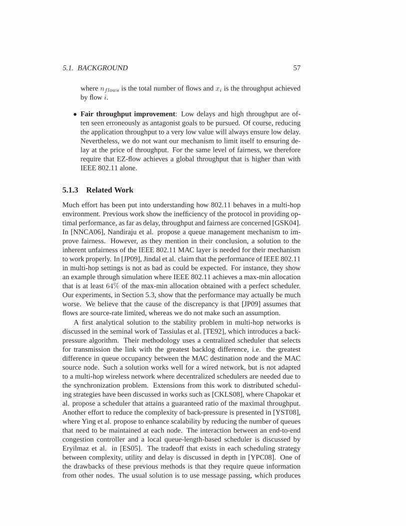
5.1. BACKGROUND 57
wherenflows is the total number of flows andxi is the throughput achievedby flow i.
• Fair throughput improvement : Low delays and high throughput are of-ten seen erroneously as antagonist goals to be pursued. Of course, reducingthe application throughput to a very low value will always ensure low delay.Nevertheless, we do not want our mechanism to limit itself to ensuring de-lay at the price of throughput. For the same level of fairness, we thereforerequire that EZ-flow achieves a global throughput that is higher than withIEEE 802.11 alone.
5.1.3 Related Work
Much effort has been put into understanding how 802.11 behaves in a multi-hopenvironment. Previous work show the inefficiency of the protocol in providing op-timal performance, as far as delay, throughput and fairness are concerned [GSK04].In [NNCA06], Nandiraju et al. propose a queue management mechanism toim-prove fairness. However, as they mention in their conclusion, a solution to theinherent unfairness of the IEEE 802.11 MAC layer is needed for their mechanismto work properly. In [JP09], Jindal et al. claim that the performance ofIEEE 802.11in multi-hop settings is not as bad as could be expected. For instance, they showan example through simulation where IEEE 802.11 achieves a max-min allocationthat is at least64% of the max-min allocation obtained with a perfect scheduler.Our experiments, in Section 5.3, show that the performance may actually be muchworse. We believe that the cause of the discrepancy is that [JP09] assumes thatflows are source-rate limited, whereas we do not make such an assumption.
A first analytical solution to the stability problem in multi-hop networks isdiscussed in the seminal work of Tassiulas et al. [TE92], which introduces a back-pressure algorithm. Their methodology uses a centralized scheduler that selectsfor transmission the link with the greatest backlog difference, i.e. the greatestdifference in queue occupancy between the MAC destination node and theMACsource node. Such a solution works well for a wired network, but is notadaptedto a multi-hop wireless network where decentralized schedulers are needed due tothe synchronization problem. Extensions from this work to distributed schedul-ing strategies have been discussed in works such as [CKLS08], whereChapokar etal. propose a scheduler that attains a guaranteed ratio of the maximal throughput.Another effort to reduce the complexity of back-pressure is presentedin [YST08],where Ying et al. propose to enhance scalability by reducing the number ofqueuesthat need to be maintained at each node. The interaction between an end-to-endcongestion controller and a local queue-length-based scheduler is discussed byEryilmaz et al. in [ES05]. The tradeoff that exists in each scheduling strategybetween complexity, utility and delay is discussed in depth in [YPC08]. One ofthe drawbacks of these previous methods is that they require queue informationfrom other nodes. The usual solution is to use message passing, which produces
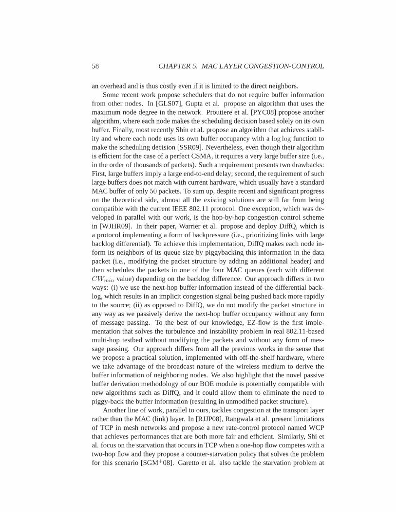
58 CHAPTER 5. MAC LAYER CONGESTION-CONTROL
an overhead and is thus costly even if it is limited to the direct neighbors.Some recent work propose schedulers that do not require buffer information
from other nodes. In [GLS07], Gupta et al. propose an algorithm that uses themaximum node degree in the network. Proutiere et al. [PYC08] propose anotheralgorithm, where each node makes the scheduling decision based solely on itsownbuffer. Finally, most recently Shin et al. propose an algorithm that achieves stabil-ity and where each node uses its own buffer occupancy with alog log function tomake the scheduling decision [SSR09]. Nevertheless, even though their algorithmis efficient for the case of a perfect CSMA, it requires a very large buffer size (i.e.,in the order of thousands of packets). Such a requirement presents twodrawbacks:First, large buffers imply a large end-to-end delay; second, the requirement of suchlarge buffers does not match with current hardware, which usually have a standardMAC buffer of only50 packets. To sum up, despite recent and significant progresson the theoretical side, almost all the existing solutions are still far from beingcompatible with the current IEEE 802.11 protocol. One exception, which wasde-veloped in parallel with our work, is the hop-by-hop congestion control schemein [WJHR09]. In their paper, Warrier et al. propose and deploy DiffQ,which isa protocol implementing a form of backpressure (i.e., prioritizing links with largebacklog differential). To achieve this implementation, DiffQ makes each node in-form its neighbors of its queue size by piggybacking this information in the datapacket (i.e., modifying the packet structure by adding an additional header) andthen schedules the packets in one of the four MAC queues (each with differentCWmin value) depending on the backlog difference. Our approach differs intwoways: (i) we use the next-hop buffer information instead of the differential back-log, which results in an implicit congestion signal being pushed back more rapidlyto the source; (ii) as opposed to DiffQ, we do not modify the packet structure inany way as we passively derive the next-hop buffer occupancy without any formof message passing. To the best of our knowledge, EZ-flow is the first imple-mentation that solves the turbulence and instability problem in real 802.11-basedmulti-hop testbed without modifying the packets and without any form of mes-sage passing. Our approach differs from all the previous works in thesense thatwe propose a practical solution, implemented with off-the-shelf hardware,wherewe take advantage of the broadcast nature of the wireless medium to derive thebuffer information of neighboring nodes. We also highlight that the novelpassivebuffer derivation methodology of our BOE module is potentially compatible withnew algorithms such as DiffQ, and it could allow them to eliminate the need topiggy-back the buffer information (resulting in unmodified packet structure).
Another line of work, parallel to ours, tackles congestion at the transport layerrather than the MAC (link) layer. In [RJJP08], Rangwala et al. presentlimitationsof TCP in mesh networks and propose a new rate-control protocol namedWCPthat achieves performances that are both more fair and efficient. Similarly,Shi etal. focus on the starvation that occurs in TCP when a one-hop flow competes with atwo-hop flow and they propose a counter-starvation policy that solves theproblemfor this scenario [SGM+08]. Garetto et al. also tackle the starvation problem at
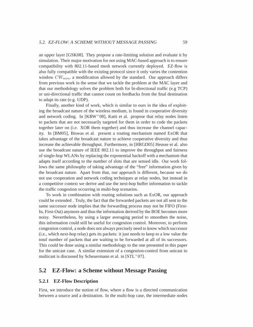
5.2. EZ-FLOW: A SCHEME WITHOUT MESSAGE PASSING 59
an upper layer [GSK08]. They propose a rate-limiting solution and evaluateit bysimulation. Their major motivation for not using MAC-based approach is to ensurecompatibility with 802.11-based mesh network currently deployed. EZ-flow isalso fully compatible with the existing protocol since it only varies the contentionwindow CWmin, a modification allowed by the standard. Our approach differsfrom previous work in the sense that we tackle the problem at the MAC layerandthat our methodology solves the problem both for bi-directional traffic (e.gTCP)or uni-directional traffic that cannot count on feedbacks from the final destinationto adapt its rate (e.g. UDP).
Finally, another kind of work, which is similar to ours in the idea of exploit-ing the broadcast nature of the wireless medium, is found in cooperative diversityand network coding. In [KRW+08], Katti et al. propose that relay nodes listento packets that are not necessarily targeted for them in order to code the packetstogether later on (i.e. XOR them together) and thus increase the channel capac-ity. In [BM05], Biswas et al. present a routing mechanism named ExOR thattakes advantage of the broadcast nature to achieve cooperative diversity and thusincrease the achievable throughput. Furthermore, in [HRGD05] Heusseet al. alsouse the broadcast nature of IEEE 802.11 to improve the throughput and fairnessof single-hop WLANs by replacing the exponential backoff with a mechanism thatadapts itself according to the number of slots that are sensed idle. Our workfol-lows the same philosophy of taking advantage of the “free” information given bythe broadcast nature. Apart from that, our approach is different, because we donot use cooperation and network coding techniques at relay nodes, but instead ina competitive context we derive and use the next-hop buffer information totacklethe traffic congestion occurring in multi-hop scenarios.
To work in combination with routing solutions such as ExOR, our approachcould be extended . Truly, the fact that the forwarded packets are notall sent to thesame successor node implies that the forwarding process may not be FIFO(First-In, First-Out) anymore and thus the information derived by the BOE becomesmorenoisy. Nevertheless, by using a larger averaging period to smoothen the noise,this information could still be useful for congestion control. Moreover, to performcongestion control, a node does not always precisely need to know which successor(i.e., which next-hop relay) gets its packets: it just needs to keep to a low value thetotal number of packets that are waiting to be forwarded at all of its successors.This could be done using a similar methodology to the one presented in this paperfor the unicast case. A similar extension of a congestion-control from unicast tomulticast is discussed by Scheuermann et al. in [STL+07].
5.2 EZ-Flow: a Scheme without Message Passing
5.2.1 EZ-Flow Description
First, we introduce the notion of flow, where a flow is a directed communicationbetween a source and a destination. In the multi-hop case, the intermediate nodes
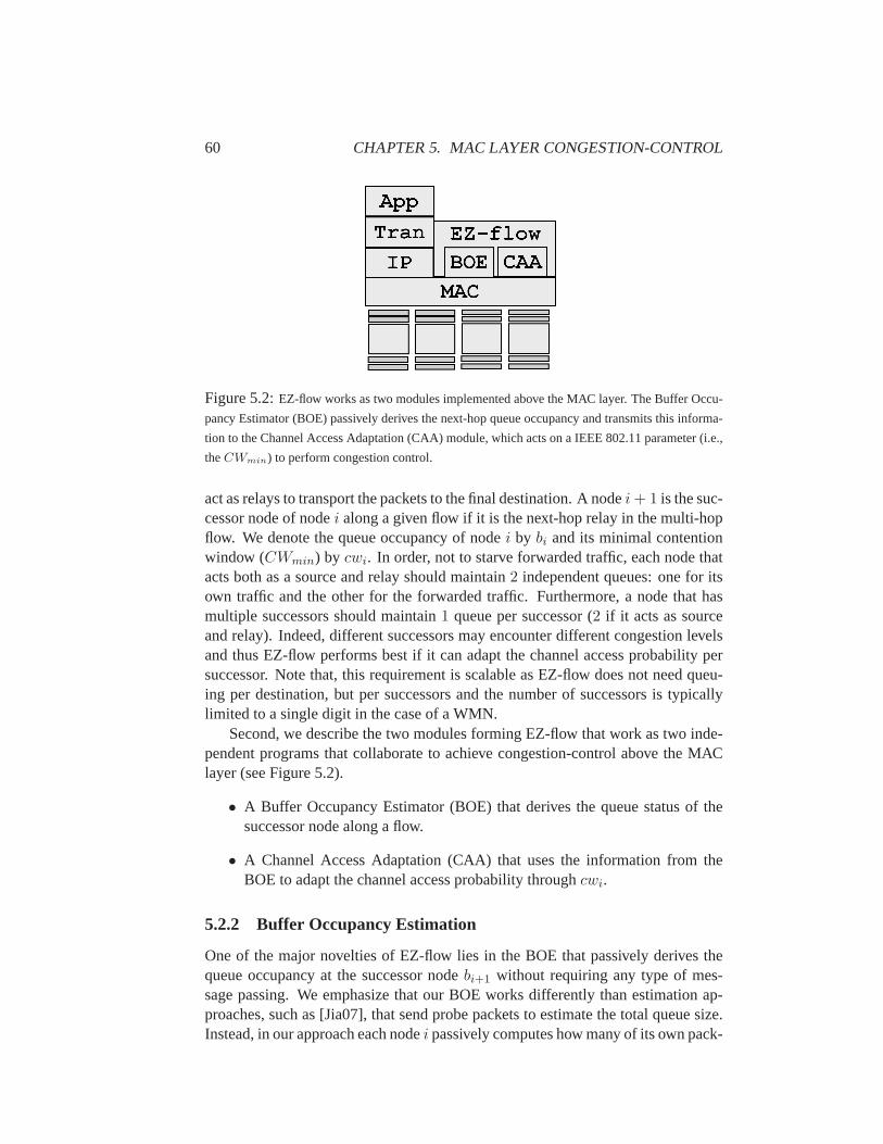
60 CHAPTER 5. MAC LAYER CONGESTION-CONTROL
Figure 5.2:EZ-flow works as two modules implemented above the MAC layer. The Buffer Occu-
pancy Estimator (BOE) passively derives the next-hop queue occupancy and transmits this informa-
tion to the Channel Access Adaptation (CAA) module, which acts on a IEEE 802.11 parameter (i.e.,
theCWmin) to perform congestion control.
act as relays to transport the packets to the final destination. A nodei+ 1 is the suc-cessor node of nodei along a given flow if it is the next-hop relay in the multi-hopflow. We denote the queue occupancy of nodei by bi and its minimal contentionwindow (CWmin) by cwi. In order, not to starve forwarded traffic, each node thatacts both as a source and relay should maintain2 independent queues: one for itsown traffic and the other for the forwarded traffic. Furthermore, a node that hasmultiple successors should maintain1 queue per successor (2 if it acts as sourceand relay). Indeed, different successors may encounter different congestion levelsand thus EZ-flow performs best if it can adapt the channel access probability persuccessor. Note that, this requirement is scalable as EZ-flow does not need queu-ing per destination, but per successors and the number of successorsis typicallylimited to a single digit in the case of a WMN.
Second, we describe the two modules forming EZ-flow that work as two inde-pendent programs that collaborate to achieve congestion-control above the MAClayer (see Figure 5.2).
• A Buffer Occupancy Estimator (BOE) that derives the queue status of thesuccessor node along a flow.
• A Channel Access Adaptation (CAA) that uses the information from theBOE to adapt the channel access probability throughcwi.
5.2.2 Buffer Occupancy Estimation
One of the major novelties of EZ-flow lies in the BOE that passively derives thequeue occupancy at the successor nodebi+1 without requiring any type of mes-sage passing. We emphasize that our BOE works differently than estimation ap-proaches, such as [Jia07], that send probe packets to estimate the total queue size.Instead, in our approach each nodei passively computes how many of its own pack-

5.2. EZ-FLOW: A SCHEME WITHOUT MESSAGE PASSING 61
ets are queued at nodei+1. Using this information, instead of the total queue size,EZ-flow aims to keep the number of packets at a successor’s queue small. This de-sign choice prevents a node from starving itself due to non-cooperativeneighbors(not performing congestion control).
To perform its task, the BOE keeps in memory a listL of the identifiers of thelast1000 packets it sent to a successor node. In our deployment we use the16-bitchecksum of the TCP or UDP packet as an identifier so as not to incur anycompu-tational overhead due to processing the packet. We note that this identifier,presentin the packet header, could be used by any mesh network based on TCP/UDP andIP, and this is clearly the standard in currently deployed networks. We stress, how-ever, that this design choice is used without any loss of generality. Even if, inthe future, the standard would be to run IPsec or to use non-TCP/UDP packets,our mechanism would instead simply need to use a lightweight hash of the packetpayload as an identifier.
Algorithm 1 EZ-flow mechanism at nodeiBOE module:if transmission of packetp to nodei+ 1 then
Store checksum ofp in PktSent[] (overwrite oldest entry if needed)LastPktSent = checksum ofp
else ifsniffing of packetp from i+ 1 to i+ 2 thenif checksum ofp ∈ PktSent[] thenbi+1 = number of packets inPktSent[] betweenp andLastPktSentreturn bi+1 to CAA module
end ifend if
CAA module:Require: Reception of50 bi+1 samples from BOEbi+1 = Average of50 bi+1 samplesif (bi+1 > bmax) then
countdown ← 0; countup ← countup + 1if (countup >= log(cwi)) thencwi ← cwi · 2; countup ← 0
end ifelse if(bi+1 < bmin) then
countup ← 0; countdown ← countdown + 1if (countdown >= 15− log(cwi)) thencwi ← cwi/2; countdown ← 0
end ifelse
countup ← 0; countdown ← 0end if
62 CHAPTER 5. MAC LAYER CONGESTION-CONTROL
The second information needed is the identifier of the packet that is actuallyforwarded by the successor node. This piece of information can be obtained bytaking advantage of the broadcast nature of the wireless medium. Indeed, nodei ison the range ofi+ 1 and is thus able to hear most of the packets that are sent bynodei+ 1 to i+ 2. In the usual settings, the MAC layer at each node transmits tothe upper layer only the messages that are targeted to it and ignores the messagestargeted to other nodes. However, by setting a node in the monitoring mode, it ispossible to sniff packets that are targeted to other nodes through a raw socket (astcpdump does1). Using such a methodology, it is then possible for a node to trackwhich packets are being forwarded by its successor node without it requiring anyform of message passing.
Finally, as the standard buffering policy is ”First In, First Out” (FIFO),nodeican accurately compute the number of its packets stored at nodei+ 1 each time ithears a packet from nodei+ 1.Indeed, it only needs to compare the identifier of the packet it hears with theiden-tifiers of the sent packets it has in the listL. The number of packets between thecorresponding match (the packet that nodei+ 1 forwards) and the last packet thatnodei sent (the last entry in the listL) corresponds tobi+1.It is important to note that, in order to perform its task, the BOE module does notneed to overhear all the packets forwarded by nodei+ 1. Instead, it is enough forit to be able to overhear some packets. Each time nodei overhears a forwardedpacket from nodei+ 1 (which happens most of the time, experimentally), it canprecisely derive the queue occupancy and transmit it to the CAA that will react ac-cordingly. Obviously, the more forwarded packets nodei can overhear, the fasterit can detect and react to congestion. Nevertheless, even in the hypothetical casewhere nodei is unable to hear most of the forwarded packets, it will still adaptto the congestion and eventually set its contention window to the right value. Thisrobustness of EZ-flow to forwarded packets that are not overheardis a crucial prop-erty, as some packets may be missed due to the variability of the wireless channelor hidden node situations.
5.2.3 Channel Access Adaptation
The second module of EZ-flow is the CAA that adapts the channel access proba-bility according tobi+1, which is the50-sample average of thebi+1 derived by theBOE. The intuition behind EZ-flow is that in the case a successor node already hasmany packets to forward, it is useless to send it more packets. Even worse, sendingmore packets degrades the performance. Indeed, every time nodei sends a newpacket to be forwarded, nodei+ 1 looses a chance to transmit.
Following this result, we propose a simple policy for the CAA that uses solelytwo thresholds: (i)bmin and (ii) bmax. Then it adapts the channel access of eachnode by changing its value of the contention windowcwi. Indeed, every time the
1The Tcpdump Manual Page: http://www.tcpdump.org/
5.2. EZ-FLOW: A SCHEME WITHOUT MESSAGE PASSING 63
nodei needs to send a packet when the channel is not idle, it randomly choosesabackoff value that is inside the interval[0, cwi − 1] and it waits for this amount oftime before retrying to transmit (see Section 2.3 for more details on IEEE 802.11).Therefore, we note that the higher thecwi is, the lower the channel access proba-bility is.
Our policy makes the decision based on a time average of the queue occupancyat the successor node (bi+1). We set the time average parameter to be50 samplesand then one of three cases may occur:
• bi+1 < bmin: the average queue at nodei+ 1 is below the lower threshold.This shows that the buffer is underutilized. Thus nodei should increase itschannel access probability by dividingcwi by a factor of two.
• bi+1 > bmax: the average queue at nodei+ 1 is above the upper threshold.This shows that the buffer is overutilized (or is even overflowing). Thusnodei should decrease its channel access probability, which it does by doublingcwi.
• bmin < bi+1 < bmax: this is the desired situation as the buffer is correctlyutilized by being neither empty most of the time nor saturated. In this case,nodei concludes that it has a correct channel access probability and thuskeepscwi unchanged.
Other policies than multiplicative-increase, multiplicative-decrease could beused to updatecwi in order to have a higher range of possible values. Yet, wechose this policy due to the hardware constraint that requires settingcwi at powersof 2.
Furthermore, we provide a better inter-flow fairness in EZ-flow by using twoparameters:
• countup counts the number of successive times the condition (bi+1 > bmax)happens (overutilization).
• countdown counts the number of successive times the condition (bi+1 <bmin) happens (underutilization).
These two pieces of information are then used to update the contention windowparameter according to the currentcwi value, where nodes with a highcwi reactboth more quickly to underutilization signals and more slowly to overutilizationsignals than nodes with a lowcwi.
Finally, the selection of the parametersbmin andbmax can affect the reactivityand the speed of convergence of EZ-flow, depending on the topology.Indeed, thesmaller the gap between these two values, the higher the reactivity of EZ-flowtoslight variations, whether due to variations of the traffic load or not. Theseparam-eters can thus be fine tuned depending on the desired behavior, but fortunately thegeneral values ofbmin andbmax already significantly improve the situation com-pared to standard IEEE 802.11. Indeed, the most important parameter to set is
64 CHAPTER 5. MAC LAYER CONGESTION-CONTROL
bmin, which has to be very small (i.e.,∼ 10−1) in order to avoid that the nodes toooften become too aggressive and reach unsupportable rates. The parameterbmax
can then be set with more flexibility, depending on the desired reactivity.
5.3 Experimental Evaluation
We implement EZ-flow and evaluate it on9 off-the-shelf wireless nodes of ourtestbed. First, we describe the environment and hardware used in our experi-ment and discuss the practical details for the implementation of EZ-flow. Then,we present the measurement results that confirm the efficiency of EZ-flow in im-proving the performance in a real WMN environment.
5.3.1 Hardware and Software Description
We use4 laptops running Linux, which act as source and sink of the traffic, and9wireless nodes equipped with an omni-directional antenna that representthe multi-hop backhaul of a mesh network. We recall that the wireless routers areAsus WL-500gP, in which we change the mini-PCI WiFi card to an NMP-8602 Atheros card.Each router runs the OpenWRT firmware [OPE] with the MadWifi driver [MAD]modified to perform both queue monitoring and the modification of the contentionwindow. The wireless cards operate in 802.11b at a fixed transmission rateof1 Mb/s and with the RTS/CTS mechanism disabled. Finally, we set the routing tobe static.
We implement the two modules of EZ-flow, the BOE and CAA, in C code asdescribed in Section 5.2. Two practical constraints need to be accounted for. Bothof them are not required in other implementations with different hardware.
1. Sniffer constraint: We initially intended to deploy both the BOE and CAAmodule within the same wireless card (i.e., the same router), but we had toreconsider our design. Indeed, the BOE acts mostly as a sniffer that collectsthe packets sent either by a node itself or its direct forwarder. The problem isthat a WiFi card cannot transmit and receive at the same time and thereforeis unable to truly sniff its own packet on the air. Instead the best a sniffercan do is to capture the packet before it is sent to the MAC layer to be ac-tually transmitted on the air. The drawback of this technique, however, isthat packets can be sniffed as sent by a node, even though they are droppedby the MAC layer (for example a buffer overflow), and thus are never re-ally physically transmitted. To overcome this limitation, we use two WiFiinterfaces per wireless node (i.e., two routers connected through an Ether-net cable). One interface is responsible for sending the traffic and runningthe CAA. The other interface does not transmit any packets and acts onlyas a sniffer that implements the BOE. We use this approach to simplify thepractical deployment. EZ-flow does not require the use of two interfaces.Indeed, another approach could be to use only one interface and to directly
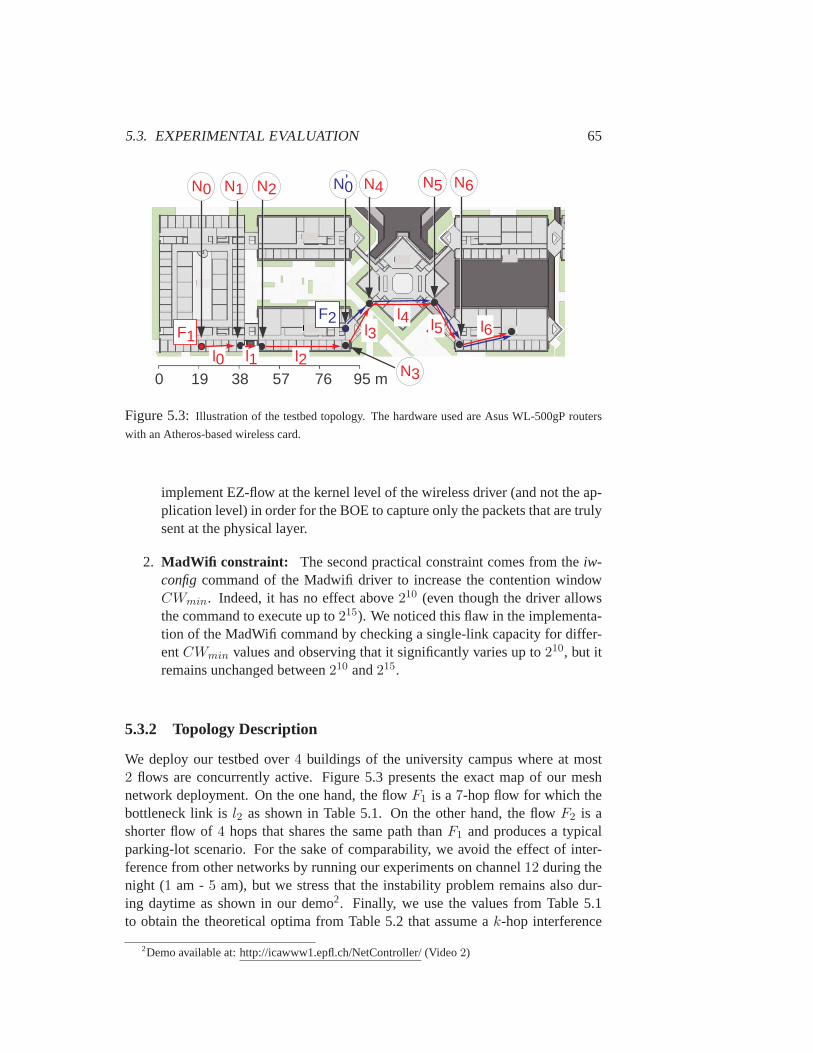
5.3. EXPERIMENTAL EVALUATION 65
F1
0 19 38 57 76 95 m
l0
l5l4
l3
l2l1
F2l6
N0 N1 N2 N4
N3
N0 N6N5'
Figure 5.3:Illustration of the testbed topology. The hardware used are Asus WL-500gP routers
with an Atheros-based wireless card.
implement EZ-flow at the kernel level of the wireless driver (and not the ap-plication level) in order for the BOE to capture only the packets that are trulysent at the physical layer.
2. MadWifi constraint: The second practical constraint comes from theiw-configcommand of the Madwifi driver to increase the contention windowCWmin. Indeed, it has no effect above210 (even though the driver allowsthe command to execute up to215). We noticed this flaw in the implementa-tion of the MadWifi command by checking a single-link capacity for differ-entCWmin values and observing that it significantly varies up to210, but itremains unchanged between210 and215.
5.3.2 Topology Description
We deploy our testbed over4 buildings of the university campus where at most2 flows are concurrently active. Figure 5.3 presents the exact map of ourmeshnetwork deployment. On the one hand, the flowF1 is a7-hop flow for which thebottleneck link isl2 as shown in Table 5.1. On the other hand, the flowF2 is ashorter flow of4 hops that shares the same path thanF1 and produces a typicalparking-lot scenario. For the sake of comparability, we avoid the effectof inter-ference from other networks by running our experiments on channel12 during thenight (1 am - 5 am), but we stress that the instability problem remains also dur-ing daytime as shown in our demo2. Finally, we use the values from Table 5.1to obtain the theoretical optima from Table 5.2 that assume ak-hop interference
2Demo available at: http://icawww1.epfl.ch/NetController/(Video2)

66 CHAPTER 5. MAC LAYER CONGESTION-CONTROL
Mean throughput Standard deviation
l0 845 kb/s 23 kb/sl1 672 kb/s 49 kb/sl2 408 kb/s 67 kb/sl3 748 kb/s 42 kb/sl4 746 kb/s 28 kb/sl5 805 kb/s 27 kb/sl6 648 kb/s 43 kb/s
Table 5.1: Illustration of the capacity of each link of flowF1. The means are obtained through
measurements over1200 s.
effect between the links withk = 2 andk = 3 (the experimental setup is some-where between this two ranges). To do so, we compute the capacity of all paths ofinterfering links
Cj+kj = 1/(
j+k∑
i=j
1
Ci) , for 0 ≤ j ≤ 6− k,
and whereCi is the capacity of linkli. The theoretical optimum is then obtained bytaking the capacityCj′+k
j′ of the bottleneck path of interfering links within a flow.
5.3.3 Measurement Results
The first scenario we consider is whenF1 is alone in the network. Figure 5.4shows the queue evolution with standard IEEE 802.11 and with EZ-flow turned on.We note that for IEEE 802.11 both nodesN1 andN2 saturate and overflow, dueto the bottleneck linkl2 (betweenN2 andN3), whereas the queue occupancy ofall the other nodes is negligibly small, similarly toN3. This results in an end-to-end throughput of119 kb/s as shown in Table 5.2 (note that a similar through-put degradation for the backlogged case has been observed throughsimulationin [LBDC+01]). In contrast, EZ-flows detects and reacts to the bottleneck at linkl2by increasingcw1 up to28. This action stabilizes the queue ofN2 by reducing thechannel access of linkl1. Similarly, EZ-flow detects that the queue ofN1 buildsup and forcesN0 to increasecw0 until it reaches our hardware limit of210 (seeSection4.1). This hardware limitation prevents EZ-flow from reducing the queueoccupancy ofN1 to a value as low asN2. However, we stress that despite thishardware limitation, EZ-flow still significantly improves the performance by re-ducing the turbulence of the flow and increasing the throughput to148 kb/s (closeto the3-hop interference range theoretical optimum and mapping to a41% reduc-tion in the gap to the2-hop optimum). Furthermore, we show through simulationin Section 5.4 that EZ-flow completely stabilizes the network once this limitationis removed.
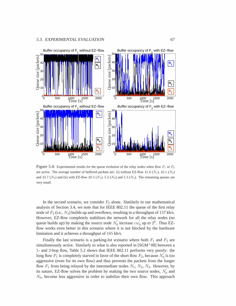
5.3. EXPERIMENTAL EVALUATION 67
0 500 1000 1500 20000
10
20
30
40
50Buffer occupancy of F
1 without EZ−flow
N2
N1
N3
Time [s]
Que
uesi
ze[p
acke
ts]
0 500 1000 1500 20000
10
20
30
40
50Buffer occupancy of F
1 with EZ−flow
N1
N2
N3
Time [s]
Que
uesi
ze[p
acke
ts]
0 500 1000 1500 20000
10
20
30
40
50Buffer occupancy of F
2 without EZ−flow
N4
N5
N6
Time [s]
Que
uesi
ze[p
acke
ts]
0 500 1000 1500 20000
10
20
30
40
50Buffer occupancy of F
2 with EZ−flow
N4
N5
N6
Time [s]
Que
uesi
ze[p
acke
ts]
Figure 5.4:Experimental results for the queue evolution of the relay nodes when flowF1 or F2
are active. The average number of buffered packets are: (i) without EZ-flow 41.6 (N1), 43.1 (N2)
and43.7 (N4) and (ii) with EZ-flow29.5 (N1), 5.2 (N2) and5.3 (N4). The remaining queues are
very small.
In the second scenario, we considerF2 alone. Similarly to our mathematicalanalysis of Section 3.4, we note that for IEEE 802.11 the queue of the firstrelaynode ofF2 (i.e.,N4) builds up and overflows, resulting in a throughput of157 kb/s.However, EZ-flow completely stabilizes the network for all the relay nodes (noqueue builds up) by making the source nodeN
′
0 increasecw′
0 up to28. Thus EZ-flow works even better in this scenario where it is not blocked by the hardwarelimitation and it achieves a throughput of185 kb/s.
Finally the last scenario is a parking-lot scenario where bothF1 andF2 aresimultaneously active. Similarly to what is also reported in [SGM+08] between a1- and2-hop flow, Table 5.2 shows that IEEE 802.11 performs very poorly: thelong flowF1 is completely starved in favor of the short flowF2, becauseN
′
0 is tooaggressive (even for its own flow) and thus prevents the packets fromthe longerflow F1 from being relayed by the intermediate nodesN1, N2, N3. However, byits nature, EZ-flow solves the problem by making the two source nodes,N
′
0 andN0, become less aggressive in order to stabilize their own flow. This approach

68 CHAPTER 5. MAC LAYER CONGESTION-CONTROL
Mean throughput Theoretical optima Jain’s Fairnessk = 3 k = 2
F1 119 kb/s 151 kb/s 190 kb/sF2 157 kb/s 183 kb/s 242 kb/sF1 7 kb/s 0.55F2 143 kb/s
FEZ1 148 kb/s 151 kb/s 190 kb/s
FEZ2 185 kb/s 183 kb/s 242 kb/s
FEZ1 71 kb/s 0.96
FEZ2 110 kb/s
Table 5.2:Measurements over1800 s with and without EZ-flow. Theoretical optima are obtained
assuming a3-hop (2-hop) interference range. The sub-division in the table shows the results for: (i)
one single flow, or (ii) two simultaneous flows.
thus solves the starvation problem and significantly increases both the aggregatethroughput ofF1 andF2 and the Jain’s fairness index.
5.3.4 Effect of Bi-Directional Traffic
EZ-flow is designed to stabilize the queues within a flow independently of theinterferences caused by other flows. In the previous sub-section, weinvestigatedthe effect of having multiple flows by looking at a setting where two separate flowsshare part of their path to reach the same destination (e.g., the gateway).
We now focus on a different scenario, where two flows take exactly oppositepaths (i.e., the destination of a flow is the source of the other flow). Toward thisgoal we use the experimental setting depicted in Figure 5.5, where the two4-hopflows areF0→4 (from node0 to node4) andF4→0 (from node4 to node0). Themeasurements show a serious throughput asymmetry in this setting. Indeed, we setthe data rate of all nodes to2 Mb/s and when first launching each flow by itself, we
w/o, RTS, w/o EZ w/o RTS, EZ RTS, w/o EZ RTS, EZb1 93 37 37 2b2 40 2 2 1b3 0 0 0 0
F0→4 102 kb/s 140 kb/s 53 kb/s 62 kb/s
b3′ 1 1 1 1b2′ 0 0 0 0b1′ 0 0 0 0
F4→0 26 kb/s 68 kb/s 34 kb/s 44 kb/s
Table 5.3:Measurements of the effect of EZ-flow on: (i) the median queue occupancy at the relay
nodes and (ii) the end-to-end throughput of the4-hop flowsF0→4 andF4→0.
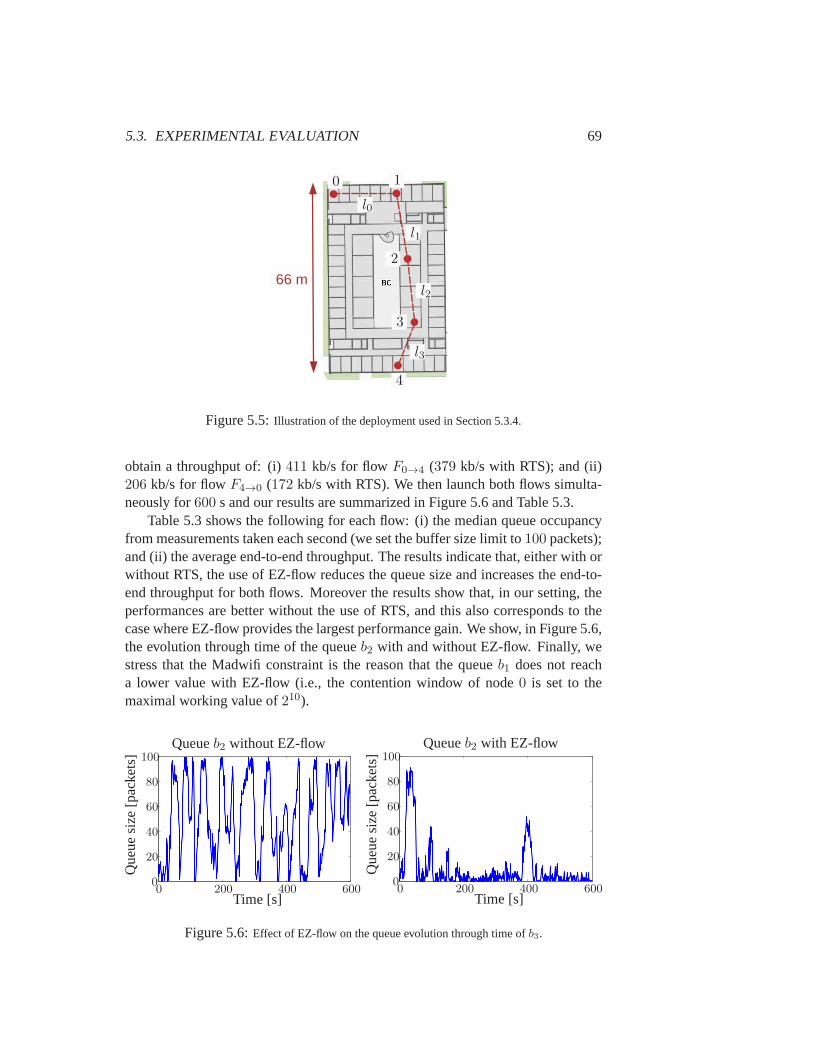
5.3. EXPERIMENTAL EVALUATION 69
66 m
0 1
2
3
4
l0
l1
l2
l3
Figure 5.5:Illustration of the deployment used in Section 5.3.4.
obtain a throughput of: (i)411 kb/s for flowF0→4 (379 kb/s with RTS); and (ii)206 kb/s for flowF4→0 (172 kb/s with RTS). We then launch both flows simulta-neously for600 s and our results are summarized in Figure 5.6 and Table 5.3.
Table 5.3 shows the following for each flow: (i) the median queue occupancyfrom measurements taken each second (we set the buffer size limit to100 packets);and (ii) the average end-to-end throughput. The results indicate that, either with orwithout RTS, the use of EZ-flow reduces the queue size and increases the end-to-end throughput for both flows. Moreover the results show that, in our setting, theperformances are better without the use of RTS, and this also corresponds to thecase where EZ-flow provides the largest performance gain. We show,in Figure 5.6,the evolution through time of the queueb2 with and without EZ-flow. Finally, westress that the Madwifi constraint is the reason that the queueb1 does not reacha lower value with EZ-flow (i.e., the contention window of node0 is set to themaximal working value of210).
Time [s]
Que
uesi
ze[p
acke
ts] Queueb2 without EZ-flow
00
20
40
60
80
100
200 400 600Time [s]
Que
uesi
ze[p
acke
ts] Queueb2 with EZ-flow
00
20
40
60
80
100
200 400 600
Figure 5.6:Effect of EZ-flow on the queue evolution through time ofb3.
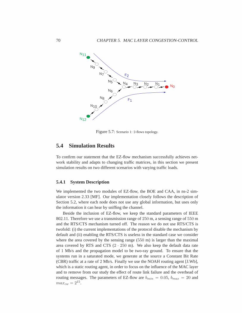
70 CHAPTER 5. MAC LAYER CONGESTION-CONTROL
F2
F1
N0
N12
N10
N8
N6
N11
N9
N7
N5 N4 N3 N2 N1
Figure 5.7:Scenario1: 2-flows topology.
5.4 Simulation Results
To confirm our statement that the EZ-flow mechanism successfully achieves net-work stability and adapts to changing traffic matrices, in this section we presentsimulation results on two different scenarios with varying traffic loads.
5.4.1 System Description
We implemented the two modules of EZ-flow, the BOE and CAA, in ns-2 sim-ulator version 2.33 [MF]. Our implementation closely follows the description ofSection 5.2, where each node does not use any global information, but uses onlythe information it can hear by sniffing the channel.
Beside the inclusion of EZ-flow, we keep the standard parameters of IEEE802.11. Therefore we use a transmission range of250 m, a sensing range of550 mand the RTS/CTS mechanism turned off. The reason we do not use RTS/CTS istwofold: (i) the current implementations of the protocol disable the mechanism bydefault and (ii) enabling the RTS/CTS is useless in the standard case we considerwhere the area covered by the sensing range (550 m) is larger than the maximalarea covered by RTS and CTS (2 · 250 m). We also keep the default data rateof 1 Mb/s and the propagation model to be two-ray ground. To ensure that thesystems run in a saturated mode, we generate at the source a Constant Bit Rate(CBR) traffic at a rate of2 Mb/s. Finally we use the NOAH routing agent [J.Wb],which is a static routing agent, in order to focus on the influence of the MAC layerand to remove from our study the effect of route link failure and the overhead ofrouting messages. The parameters of EZ-flow arebmin = 0.05, bmax = 20 andmaxcw = 215.
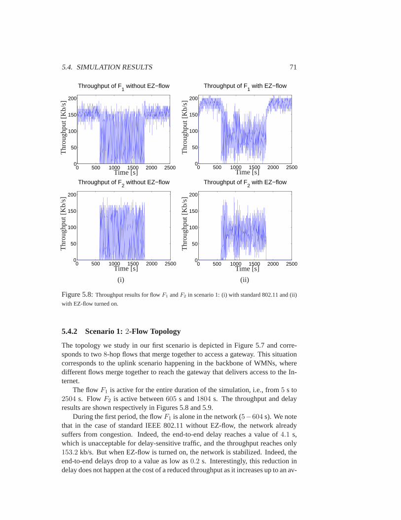
5.4. SIMULATION RESULTS 71
0 500 1000 1500 2000 25000
50
100
150
200
Throughput of F1 without EZ−flow
Time [s]
Thr
ough
put[
Kb/
s]
0 500 1000 1500 2000 25000
50
100
150
200
Throughput of F1 with EZ−flow
Time [s]
Thr
ough
put[
Kb/
s]
0 500 1000 1500 2000 25000
50
100
150
200
Throughput of F2 without EZ−flow
Time [s]
Thr
ough
put[
Kb/
s]
0 500 1000 1500 2000 25000
50
100
150
200
Throughput of F2 with EZ−flow
Time [s]
Thr
ough
put[
Kb/
s]
(i) (ii)
Figure 5.8:Throughput results for flowF1 andF2 in scenario 1: (i) with standard 802.11 and (ii)
with EZ-flow turned on.
5.4.2 Scenario 1:2-Flow Topology
The topology we study in our first scenario is depicted in Figure 5.7 and corre-sponds to two8-hop flows that merge together to access a gateway. This situationcorresponds to the uplink scenario happening in the backbone of WMNs,wheredifferent flows merge together to reach the gateway that delivers access to the In-ternet.
The flowF1 is active for the entire duration of the simulation, i.e., from5 s to2504 s. FlowF2 is active between605 s and1804 s. The throughput and delayresults are shown respectively in Figures 5.8 and 5.9.
During the first period, the flowF1 is alone in the network (5−604 s). We notethat in the case of standard IEEE 802.11 without EZ-flow, the network alreadysuffers from congestion. Indeed, the end-to-end delay reaches a value of4.1 s,which is unacceptable for delay-sensitive traffic, and the throughput reaches only153.2 kb/s. But when EZ-flow is turned on, the network is stabilized. Indeed, theend-to-end delays drop to a value as low as0.2 s. Interestingly, this reduction indelay does not happen at the cost of a reduced throughput as it increases up to an av-
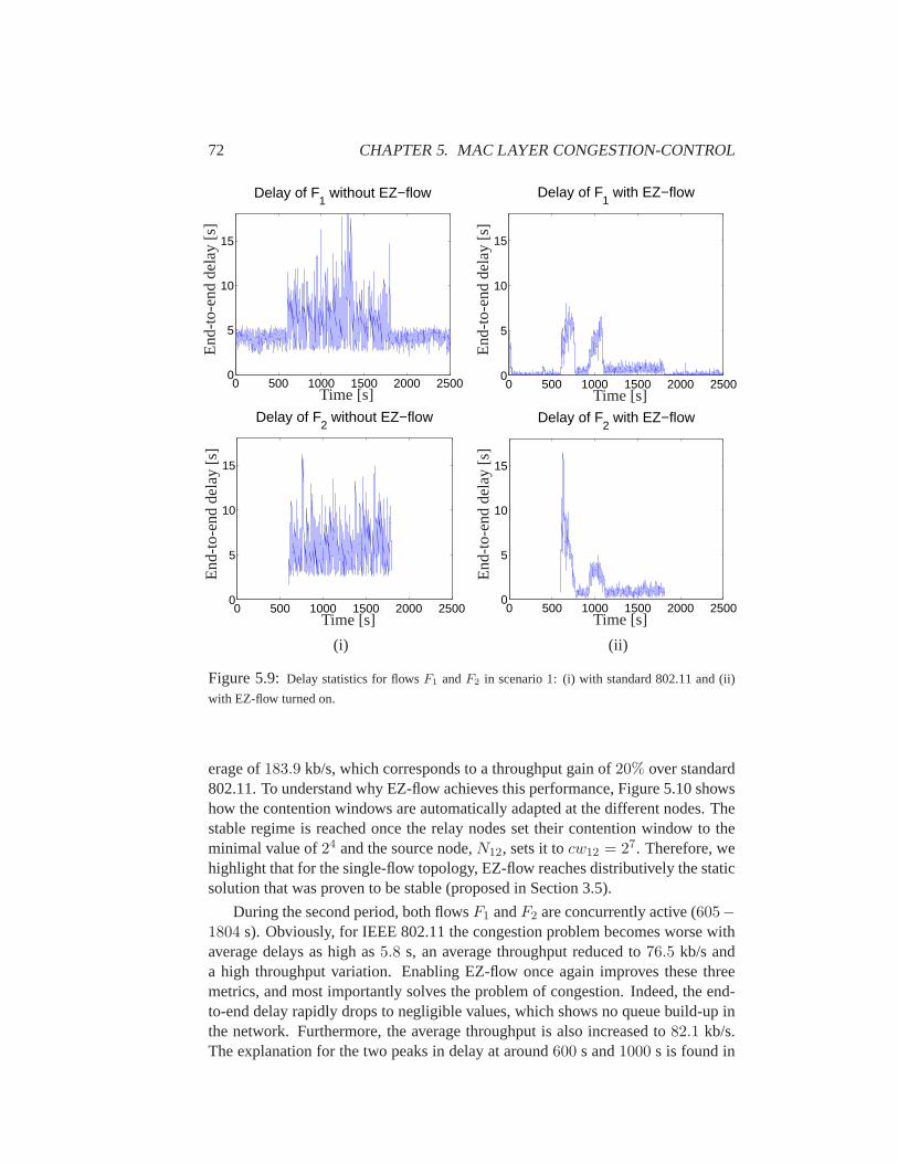
72 CHAPTER 5. MAC LAYER CONGESTION-CONTROL
0 500 1000 1500 2000 25000
5
10
15
Delay of F1 without EZ−flow
Time [s]
End
-to-
end
dela
y[s
]
0 500 1000 1500 2000 25000
5
10
15
Delay of F1 with EZ−flow
Time [s]
End
-to-
end
dela
y[s
]
0 500 1000 1500 2000 25000
5
10
15
Delay of F2 without EZ−flow
Time [s]
End
-to-
end
dela
y[s
]
0 500 1000 1500 2000 25000
5
10
15
Delay of F2 with EZ−flow
Time [s]
End
-to-
end
dela
y[s
]
(i) (ii)
Figure 5.9:Delay statistics for flowsF1 andF2 in scenario1: (i) with standard 802.11 and (ii)
with EZ-flow turned on.
erage of183.9 kb/s, which corresponds to a throughput gain of20% over standard802.11. To understand why EZ-flow achieves this performance, Figure5.10 showshow the contention windows are automatically adapted at the different nodes. Thestable regime is reached once the relay nodes set their contention window to theminimal value of24 and the source node,N12, sets it tocw12 = 27. Therefore, wehighlight that for the single-flow topology, EZ-flow reaches distributivelythe staticsolution that was proven to be stable (proposed in Section 3.5).
During the second period, both flowsF1 andF2 are concurrently active (605−1804 s). Obviously, for IEEE 802.11 the congestion problem becomes worse withaverage delays as high as5.8 s, an average throughput reduced to76.5 kb/s anda high throughput variation. Enabling EZ-flow once again improves these threemetrics, and most importantly solves the problem of congestion. Indeed, the end-to-end delay rapidly drops to negligible values, which shows no queue build-up inthe network. Furthermore, the average throughput is also increased to82.1 kb/s.The explanation for the two peaks in delay at around600 s and1000 s is found in
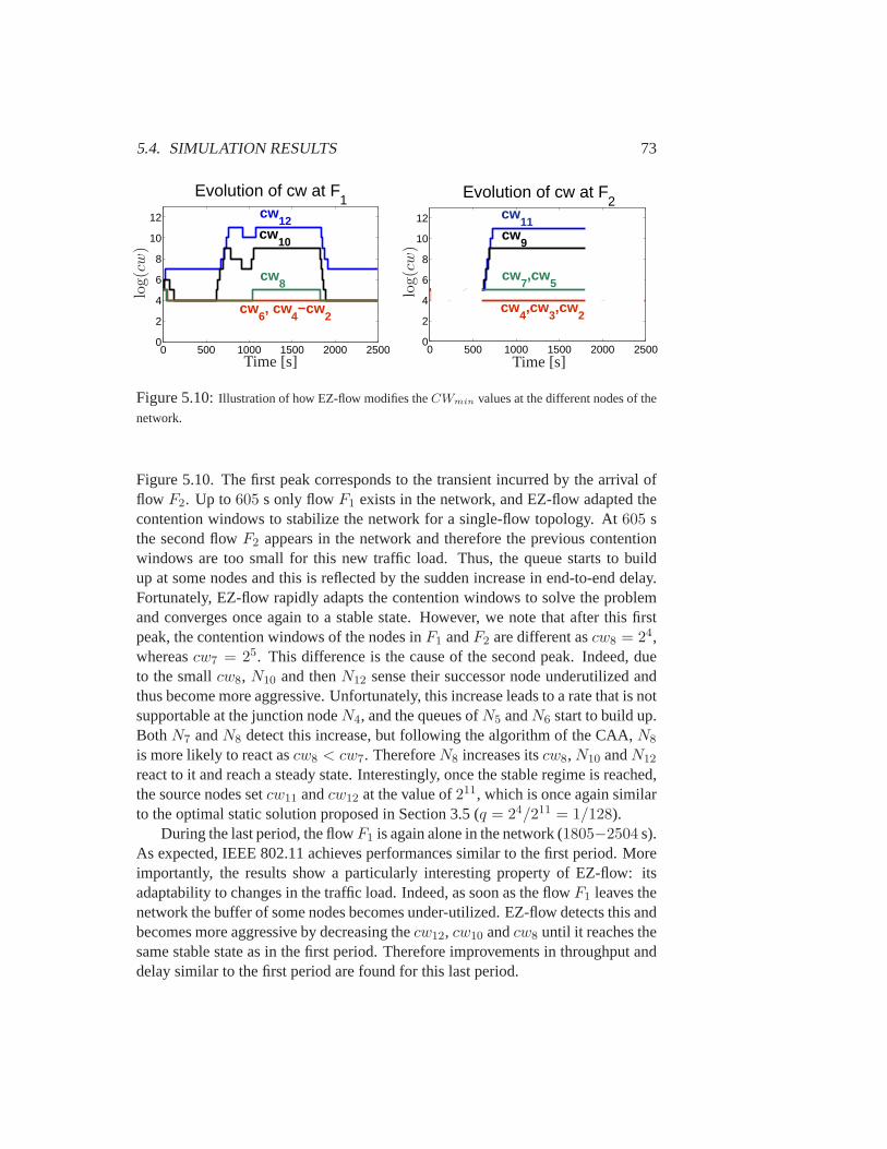
5.4. SIMULATION RESULTS 73
0 500 1000 1500 2000 25000
2
4
6
8
10
12
Evolution of cw at F1
cw10
cw12
cw8
cw6, cw
4−cw
2
Time [s]
log(cw)
0 500 1000 1500 2000 25000
2
4
6
8
10
12
Evolution of cw at F2
cw4,cw
3,cw
2
cw9
cw11
cw7,cw
5
Time [s]
log(cw)
Figure 5.10:Illustration of how EZ-flow modifies theCWmin values at the different nodes of the
network.
Figure 5.10. The first peak corresponds to the transient incurred by the arrival offlow F2. Up to605 s only flowF1 exists in the network, and EZ-flow adapted thecontention windows to stabilize the network for a single-flow topology. At605 sthe second flowF2 appears in the network and therefore the previous contentionwindows are too small for this new traffic load. Thus, the queue starts to buildup at some nodes and this is reflected by the sudden increase in end-to-end delay.Fortunately, EZ-flow rapidly adapts the contention windows to solve the problemand converges once again to a stable state. However, we note that after this firstpeak, the contention windows of the nodes inF1 andF2 are different ascw8 = 24,whereascw7 = 25. This difference is the cause of the second peak. Indeed, dueto the smallcw8, N10 and thenN12 sense their successor node underutilized andthus become more aggressive. Unfortunately, this increase leads to a ratethat is notsupportable at the junction nodeN4, and the queues ofN5 andN6 start to build up.BothN7 andN8 detect this increase, but following the algorithm of the CAA,N8
is more likely to react ascw8 < cw7. ThereforeN8 increases itscw8, N10 andN12
react to it and reach a steady state. Interestingly, once the stable regime is reached,the source nodes setcw11 andcw12 at the value of211, which is once again similarto the optimal static solution proposed in Section 3.5 (q = 24/211 = 1/128).
During the last period, the flowF1 is again alone in the network (1805−2504 s).As expected, IEEE 802.11 achieves performances similar to the first period. Moreimportantly, the results show a particularly interesting property of EZ-flow: itsadaptability to changes in the traffic load. Indeed, as soon as the flowF1 leaves thenetwork the buffer of some nodes becomes under-utilized. EZ-flow detects this andbecomes more aggressive by decreasing thecw12, cw10 andcw8 until it reaches thesame stable state as in the first period. Therefore improvements in throughput anddelay similar to the first period are found for this last period.
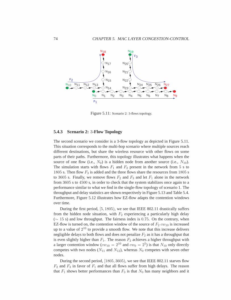
74 CHAPTER 5. MAC LAYER CONGESTION-CONTROL
F2
F3
N9N0 N7N5
N10
N8N6N4N3N2N1
F1
N11 N12 N13N14
N15
N16
N17 N20
N21
N22
N23N24 N25 N26
N19N18
N27
Figure 5.11:Scenario2: 3-flows topology.
5.4.3 Scenario 2:3-Flow Topology
The second scenario we consider is a3-flow topology as depicted in Figure 5.11.This situation corresponds to the multi-hop scenario where multiple sources reachdifferent destinations, but share the wireless resource with other flowson someparts of their paths. Furthermore, this topology illustrates what happens when thesource of one flow (i.e.,N0) is a hidden node from another source (i.e.,N10).The simulation starts with flowsF1 andF2 present in the network from5 s to1805 s. Then flowF3 is added and the three flows share the resources from1805 sto 3605 s. Finally, we remove flowsF2 andF3 and letF1 alone in the networkfrom 3605 s to4500 s, in order to check that the system stabilizes once again to aperformance similar to what we find in the single-flow topology of scenario 1.Thethroughput and delay statistics are shown respectively in Figure 5.13 andTable 5.4.Furthermore, Figure 5.12 illustrates how EZ-flow adapts the contention windowsover time.
During the first period,[5, 1805), we see that IEEE 802.11 drastically suffersfrom the hidden node situation, withF2 experiencing a particularly high delay(∼ 15 s) and low throughput. The fairness index is0.75. On the contrary, whenEZ-flow is turned on, the contention window of the source ofF2 cw10 is increasedup to a value of210 to provide a smooth flow. We note that this increase deliversnegligible delays to both flows and does not penalizeF2 as it has a throughput thatis even slightly higher thanF1. The reasonF2 achieves a higher throughput witha larger contention window (cw10 = 210 andcw0 = 25) is thatN10 only directlycompetes with two nodes (N11 andN12), whereasN0 competes with seven othernodes.
During the second period,[1805, 3605), we see that IEEE 802.11 starves flowF2 andF3 in favor of F1 and that all flows suffer from high delays. The reasonthatF1 shows better performances thanF3 is thatN0 has many neighbors and it
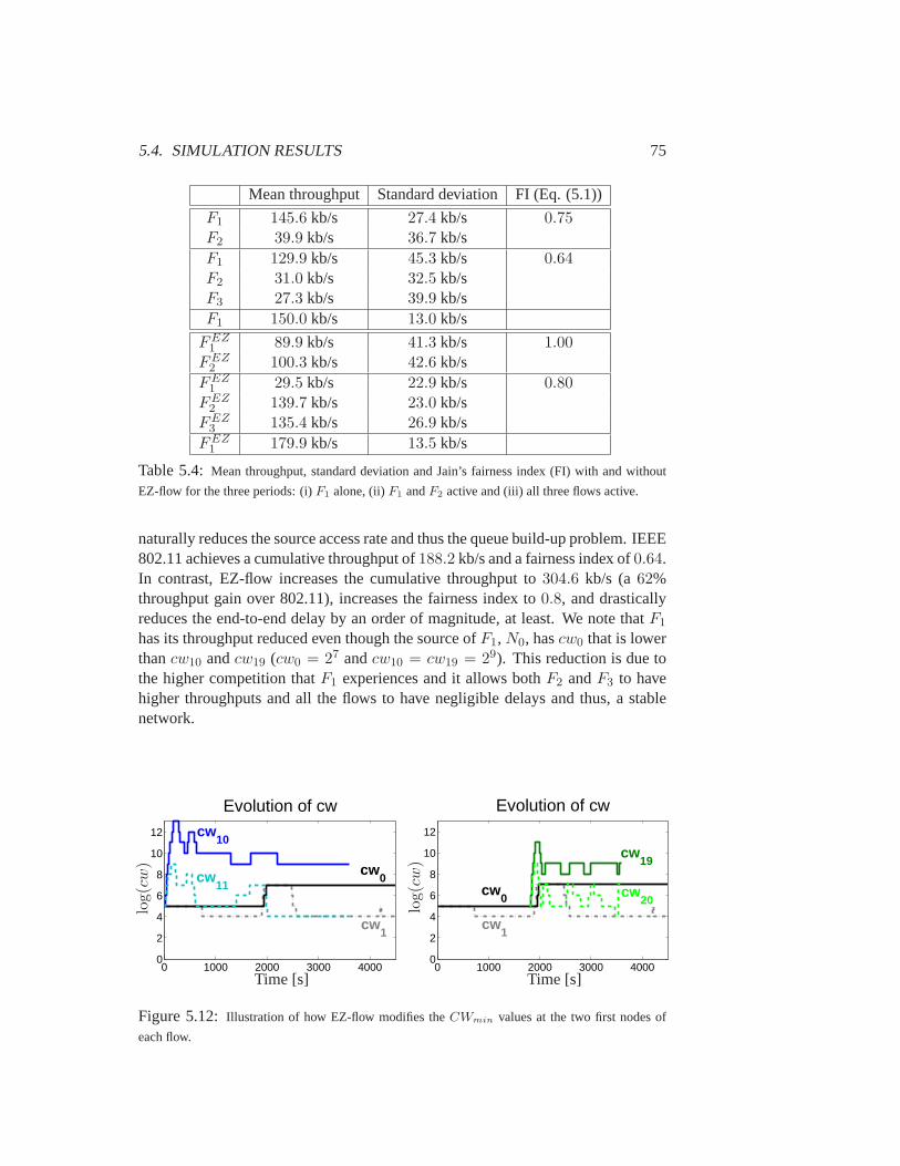
5.4. SIMULATION RESULTS 75
Mean throughput Standard deviation FI (Eq. (5.1))
F1 145.6 kb/s 27.4 kb/s 0.75F2 39.9 kb/s 36.7 kb/sF1 129.9 kb/s 45.3 kb/s 0.64F2 31.0 kb/s 32.5 kb/sF3 27.3 kb/s 39.9 kb/sF1 150.0 kb/s 13.0 kb/s
FEZ1 89.9 kb/s 41.3 kb/s 1.00
FEZ2 100.3 kb/s 42.6 kb/s
FEZ1 29.5 kb/s 22.9 kb/s 0.80
FEZ2 139.7 kb/s 23.0 kb/s
FEZ3 135.4 kb/s 26.9 kb/s
FEZ1 179.9 kb/s 13.5 kb/s
Table 5.4:Mean throughput, standard deviation and Jain’s fairness index (FI) withand without
EZ-flow for the three periods: (i)F1 alone, (ii)F1 andF2 active and (iii) all three flows active.
naturally reduces the source access rate and thus the queue build-up problem. IEEE802.11 achieves a cumulative throughput of188.2 kb/s and a fairness index of0.64.In contrast, EZ-flow increases the cumulative throughput to304.6 kb/s (a62%throughput gain over 802.11), increases the fairness index to0.8, and drasticallyreduces the end-to-end delay by an order of magnitude, at least. We notethatF1
has its throughput reduced even though the source ofF1, N0, hascw0 that is lowerthancw10 andcw19 (cw0 = 27 andcw10 = cw19 = 29). This reduction is due tothe higher competition thatF1 experiences and it allows bothF2 andF3 to havehigher throughputs and all the flows to have negligible delays and thus, a stablenetwork.
0 1000 2000 3000 40000
2
4
6
8
10
12
Evolution of cw
cw0
cw1
cw10
cw11
Time [s]
log(cw)
0 1000 2000 3000 40000
2
4
6
8
10
12
Evolution of cw
cw20
cw0
cw1
cw19
Time [s]
log(cw)
Figure 5.12:Illustration of how EZ-flow modifies theCWmin values at the two first nodes of
each flow.
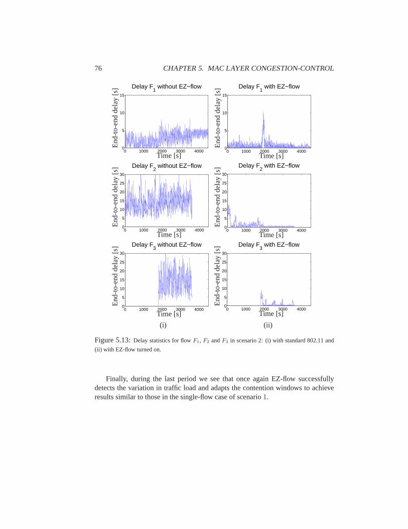
76 CHAPTER 5. MAC LAYER CONGESTION-CONTROL
0 1000 2000 3000 40000
5
10
15
Delay F1 without EZ−flow
Time [s]
End
-to-
end
dela
y[s
]
0 1000 2000 3000 40000
5
10
15
Delay F1 with EZ−flow
Time [s]
End
-to-
end
dela
y[s
]
0 1000 2000 3000 40000
5
10
15
20
25
30
Delay F2 without EZ−flow
Time [s]
End
-to-
end
dela
y[s
]
0 1000 2000 3000 40000
5
10
15
20
25
30
Delay F2 with EZ−flow
Time [s]
End
-to-
end
dela
y[s
]
0 1000 2000 3000 40000
5
10
15
20
25
30
Delay F3 without EZ−flow
Time [s]
End
-to-
end
dela
y[s
]
0 1000 2000 3000 40000
5
10
15
20
25
30
Delay F3 with EZ−flow
Time [s]
End
-to-
end
dela
y[s
]
(i) (ii)
Figure 5.13:Delay statistics for flowF1, F2 andF3 in scenario 2: (i) with standard 802.11 and
(ii) with EZ-flow turned on.
Finally, during the last period we see that once again EZ-flow successfullydetects the variation in traffic load and adapts the contention windows to achieveresults similar to those in the single-flow case of scenario1.

5.5. DYNAMICAL MODEL 77
5.5 Dynamical Model
5.5.1 EZ-Flow Dynamics
Using the same notation as in Chapter 3, the dynamics of a network using EZ-floware captured by the recursive equations
cwi(n+ 1) = f(cwi(n), bi+1(n)) (5.2)
bi(n+ 1) = bi(n) + zi−1(n)− zi(n), (5.3)
wheref(·, ·) is defined by
f(cwi(n), bi+1(n)) =
min(cwi(n) · 2,maxcw) if (bi+1(n) > bmax)max(cwi(n)/2,mincw) if (bi+1(n) < bmin)cwi(n) otherwise,
with bmax andbmin being, respectively, the maximal and minimal threshold valuesfor the queue andmincw = 2m andmaxcw = 2M being the bounds between whichthe contention windows can evolve. Practical values arem = 4 andM = 15, thuswe always take
M > m+ 1.
This discrete-time model is a Markov chain with the tuple
{~b(n), ~cw(n)}
as state, where~b(n) ∈ N
K+1
and where~cw(n) satisfies both
cwi(n) ∈ {2m, 2m+1, · · · , 2M}
and
cwi(n) ≥ 2m+min(l,M−m) whenbi+1(n) > bmax + l, (5.4)
wherel > 0. The lower-bound condition (5.4) comes from the recursive applica-tion of (5.2) for the lastl time slots. Indeed,bi+1(k) > bmax for n − l < k ≤ nimplies thatcwi(k + 1) = min(cwi(k) · 2, 2
M ).The state space is divided in2K−1 regions, which differ by the entries of~b
that are zero and non-zero (i.e., the queues that are empty or not). Figure 3.7illustrates these8 regions for a4-hop network (denotedA-H). In each region, onecan compute first the possible outcomes of the back-off timers that depend on thecontention values~cw(n), and next the resulting transmission patterns that dependalso on the possible collisions due to hidden terminals. The possible outcomes areobtained by following the same reasoning as in Section 3.4. We summarize themin Table 5.5 for the4-hop network with a stealing effectp = 1 (i.e. no RTS/CTS).

78 CHAPTER 5. MAC LAYER CONGESTION-CONTROL
Region ~z P(~z)
A [1, 0, 0, 0] 1
B [1, 0, 0, 0] cw1/(cw0 + cw1)[0, 1, 0, 0] cw0/(cw0 + cw1)
C [0, 0, 1, 0] 1
D [0, 1, 0, 0] cw0cw2∑i=0,1,2
∏j 6=i cwj
[0, 0, 1, 0] 1− cw0cw2∑i=0,1,2
∏j 6=i cwj
E [1, 0, 0, 1] 1
F [0, 0, 0, 1] cw0/(cw0 + cw1)[1, 0, 0, 1] cw1/(cw0 + cw1)
G [0, 0, 1, 0] cw3/(cw2 + cw3)[1, 0, 0, 1] cw2/(cw2 + cw3)
H [0, 0, 1, 0] cw0cw1cw3∑i=0,1,2,3
∏j 6=i cwj
+ cw1cw2cw3∑i=0,1,2,3
∏j 6=i cwj
cw3cw2+cw3
[0, 0, 0, 1] cw0cw2cw3∑i=0,1,2,3
∏j 6=i cwj
+ cw0cw1cw2∑i=0,1,2,3
∏j 6=i cwj
cw0cw0+cw1
[1, 0, 0, 1] cw1cw2cw3∑i=0,1,2,3
∏j 6=i cwj
cw2cw2+cw3
+ cw0cw1cw2∑i=0,1,2,3
∏j 6=i cwj
cw1cw0+cw1
Table 5.5:Probability of occurrence of the transmission pattern~z for the different regions of the
spaceN3.
5.5.2 Proof of Stability
Equipped with the model described above, we now formally prove the efficiencyof EZ-flow in stabilizing the network. We give a proof, which holds when
bmin > M −m+ 1. (5.5)
This condition further reduces the state space of our model as, following asimilarrecursive argument than for (5.4), it implies that
cwi(n) = 2m whenbi+1(n) = 0. (5.6)
Whenbmin ≤M −m+ 1, the proof uses computer-assisted computations, and isgiven in [ASTEF09].
Theorem 5.1 EZ-flow stabilizes a4-hop network by maintaining almost surely fi-nite the queues of all the relaying nodes.
Proof: We apply Foster’s theorem (see Appendix A) with the Lyapunov function
h(b1, b2, b3, cw0, cw1, cw2, cw3) = b1 + b2 + b3,
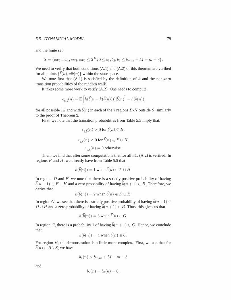
5.5. DYNAMICAL MODEL 79
and the finite set
S = {cw0, cw1, cw2, cw3 ≤ 2M ; 0 ≤ b1, b2, b3 ≤ bmax +M −m+ 3}.
We need to verify that both conditions (A.1) and (A.2) of this theorem are verifiedfor all points{~b(n), ~cw(n)} within the state space.
We note first that (A.1) is satisfied by the definition ofh and the non-zerotransition probabilities of the random walk.
It takes some more work to verify (A.2). One needs to compute
ǫk,~b
(n) = E
[
h(~b(n+ k(~b(n))))|~b(n)]
− h(~b(n))
for all possible~cw and with~b(n) in each of the7 regionsB-H outsideS, similarlyto the proof of Theorem2.
First, we note that the transition probabilities from Table 5.5 imply that:
ǫ1,~b(n) > 0 for~b(n) ∈ B,
ǫ1,~b(n) < 0 for~b(n) ∈ F ∪H,
ǫ1,~b(n) = 0 otherwise.
Then, we find that after some computations that for all~cw, (A.2) is verified. InregionsF andH, we directly have from Table 5.5 that
k(~b(n)) = 1 when~b(n) ∈ F ∪H.
In regionsD andE, we note that there is a strictly positive probability of having~b(n+ 1) ∈ F ∪H and a zero probability of having~b(n + 1) ∈ B. Therefore, wederive that
k(~b(n)) = 2 when~b(n) ∈ D ∪ E.
In regionG, we see that there is a strictly positive probability of having~b(n+1) ∈D ∪H and a zero probability of having~b(n+ 1) ∈ B. Thus, this gives us that
k(~b(n)) = 3 when~b(n) ∈ G.
In regionC, there is a probability1 of having~b(n+ 1) ∈ G. Hence, we concludethat
k(~b(n)) = 4 when~b(n) ∈ C.
For regionB, the demonstration is a little more complex. First, we use that for~b(n) ∈ B \ S, we have
b1(n) > bmax +M −m+ 3
andb2(n) = b3(n) = 0.
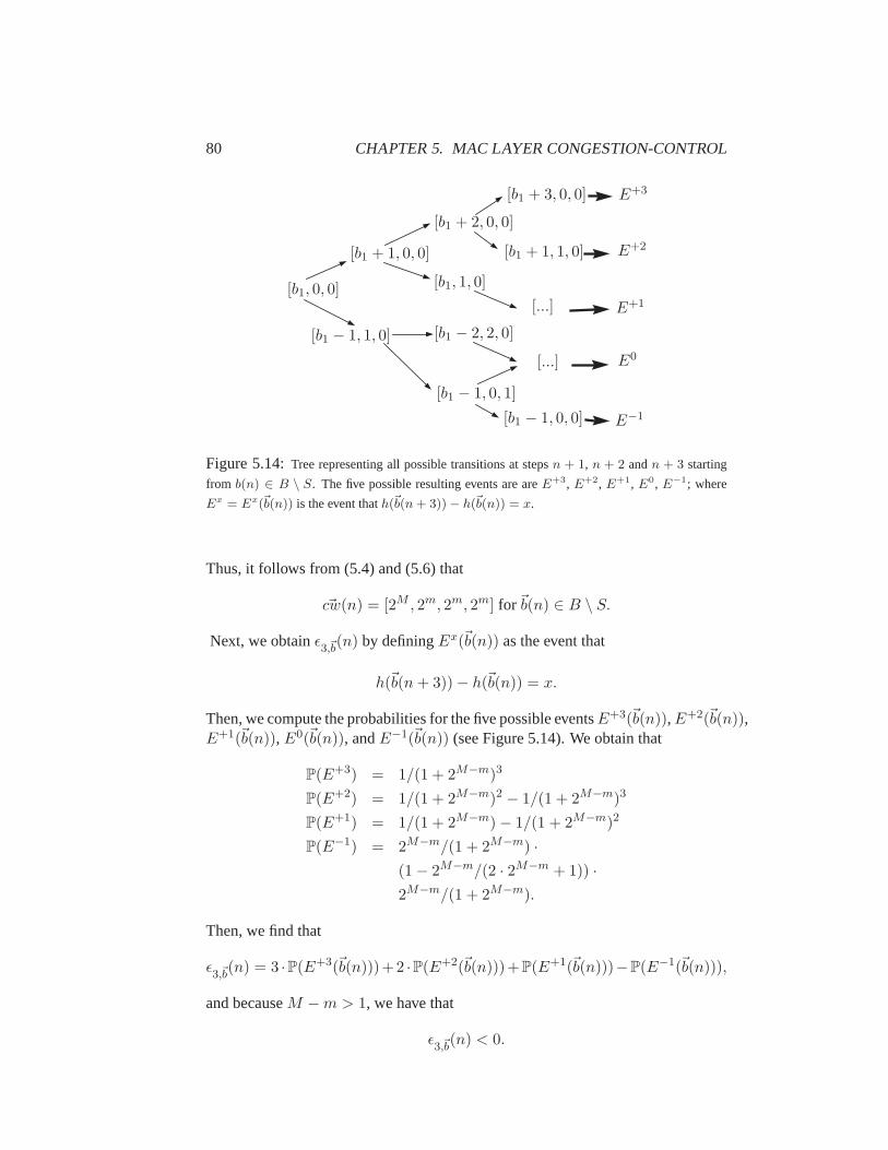
80 CHAPTER 5. MAC LAYER CONGESTION-CONTROL
[...]
[...]
E+3
E+2
E+1
E0
E−1
[b1, 0, 0][b1, 1, 0]
[b1 + 1, 1, 0][b1 + 1, 0, 0]
[b1 + 2, 0, 0]
[b1 + 3, 0, 0]
[b1 − 1, 0, 0]
[b1 − 1, 1, 0]
[b1 − 1, 0, 1]
[b1 − 2, 2, 0]
Figure 5.14:Tree representing all possible transitions at stepsn + 1, n + 2 andn + 3 starting
from b(n) ∈ B \ S. The five possible resulting events are areE+3, E+2, E+1, E0, E−1; where
Ex = Ex(~b(n)) is the event thath(~b(n+ 3))− h(~b(n)) = x.
Thus, it follows from (5.4) and (5.6) that
~cw(n) = [2M , 2m, 2m, 2m] for~b(n) ∈ B \ S.
Next, we obtainǫ3,~b(n) by definingEx(~b(n)) as the event that
h(~b(n+ 3))− h(~b(n)) = x.
Then, we compute the probabilities for the five possible eventsE+3(~b(n)),E+2(~b(n)),E+1(~b(n)), E0(~b(n)), andE−1(~b(n)) (see Figure 5.14). We obtain that
P(E+3) = 1/(1 + 2M−m)3
P(E+2) = 1/(1 + 2M−m)2 − 1/(1 + 2M−m)3
P(E+1) = 1/(1 + 2M−m)− 1/(1 + 2M−m)2
P(E−1) = 2M−m/(1 + 2M−m) ·
(1− 2M−m/(2 · 2M−m + 1)) ·
2M−m/(1 + 2M−m).
Then, we find that
ǫ3,~b(n) = 3 ·P(E+3(~b(n)))+2 ·P(E+2(~b(n)))+P(E+1(~b(n)))−P(E−1(~b(n))),
and becauseM −m > 1, we have that
ǫ3,~b(n) < 0.
5.6. CONCLUDING REMARKS 81
Thusk(~b(n)) = 3 satisfies (A.2) for~b(n) ∈ B \ S.
Finally, as RegionA ⊆ S, the conditions of Foster’s theorem are satisfied in all{~b(n), ~cw(n)} within the state space, and it proves that EZ-flow stabilizes the net-work.�
5.6 Concluding Remarks
In this chapter, we proposed and designed EZ-flow, a new flow controlmechanismfor IEEE 802.11 WMNs. EZ-flow is fully backward-compatible with the IEEE802.11 standard and works without any form of message passing. EZ-flow is im-plemented in a distributed fashion as a simple program running at each relay node.It takes advantage of the broadcast nature of the wireless medium to passivelyestimate the queue occupancy at a successor node. The minimum congestionwin-dow parameter is adapted at each relay node based on this estimation to ensure asmooth flow, specifically, each relay node adapts its contention window to avoidqueue build-up at its successor node.
We demonstrated by experiments the attendant benefits of EZ-flow on a testbedcomposed of9 standard wireless mesh routers deployed over4 different buildings.Our measurement results show that EZ-flow simultaneously improves throughputand fairness performance. To our knowledge, this is among the first implementa-tions of an algorithm addressing instability in a real multi-hop network.
We have also thoroughly evaluated the dynamic behavior of EZ-flow by usingns-2 simulation. The results show that EZ-flow quickly adapts to changing traf-fic loads and ensures end-to-end delays much lower than standard IEEE802.11WMNs.
Finally, we derived a Lyapunov function with which we analytically proved thestability of an IEEE 802.11-based linear4-hop topology implementing EZ-flow.

82 CHAPTER 5. MAC LAYER CONGESTION-CONTROL
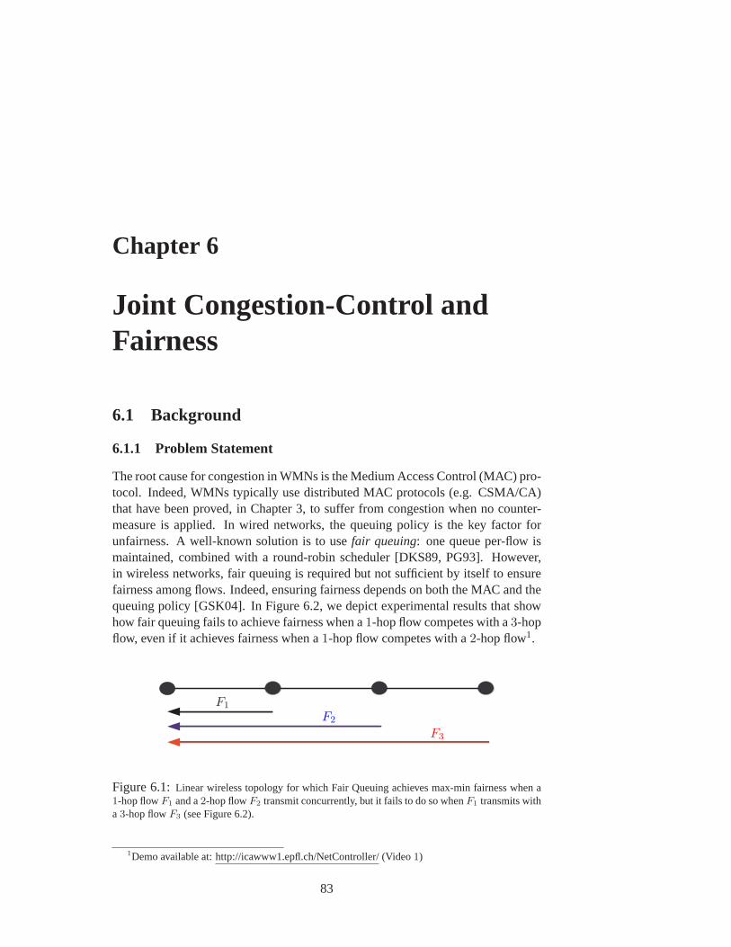
Chapter 6
Joint Congestion-Control andFairness
6.1 Background
6.1.1 Problem Statement
The root cause for congestion in WMNs is the Medium Access Control (MAC) pro-tocol. Indeed, WMNs typically use distributed MAC protocols (e.g. CSMA/CA)that have been proved, in Chapter 3, to suffer from congestion when no counter-measure is applied. In wired networks, the queuing policy is the key factor forunfairness. A well-known solution is to usefair queuing: one queue per-flow ismaintained, combined with a round-robin scheduler [DKS89, PG93]. However,in wireless networks, fair queuing is required but not sufficient by itselfto ensurefairness among flows. Indeed, ensuring fairness depends on both theMAC and thequeuing policy [GSK04]. In Figure 6.2, we depict experimental results that showhow fair queuing fails to achieve fairness when a1-hop flow competes with a3-hopflow, even if it achieves fairness when a1-hop flow competes with a2-hop flow1.
F1
F3
F2
Figure 6.1:Linear wireless topology for which Fair Queuing achieves max-min fairness when a1-hop flowF1 and a2-hop flowF2 transmit concurrently, but it fails to do so whenF1 transmits witha3-hop flowF3 (see Figure 6.2).
1Demo available at: http://icawww1.epfl.ch/NetController/(Video1)
83

84 CHAPTER 6. JOINT CONGESTION-CONTROL AND FAIRNESS
0 10 20 30 40 50 600
200
400
600
800
Time [s]
flow F1
flow F2
Thr
ough
put[
Kb/
s]1-hop vs.2-hop with FIFO
0 10 20 30 40 50 600
200
400
600
800
flow F1
Time [s]
flow F2
Thr
ough
put[
Kb/
s]
1-hop vs.2-hop with Fair Queuing
(a) (b)
0 10 20 30 40 50 600
200
400
600
800
flow F1
Time [s]
flow F3
Thr
ough
put[
Kb/
s]
1-hop vs.3-hop with FIFO
0 10 20 30 40 50 600
200
400
600
800
flow F1
Time [s]
flow F3
Thr
ough
put[
Kb/
s]
1-hop vs.3-hop with Fair Queuing
(c) (d)
Figure 6.2: End-to-end throughput in a line topology (see Figure 6.1) with a single-hop and amulti-hop UDP flow (2- or 3-hop) with the standard FIFO policy (left) and with fair queuing (right).Fair queuing achieves max-min fairness for the2-hop case (see video1), but fails to prevent starvationin the3-hop case. Results in the top-right picture (b) look identical, but it is only anartifact of thescale of the picture. Smaller scale plots show differences.
Our goal in this chapter is to address both intra-flow congestion and inter-flowfairness for the backhaul of a WMN. In addition, we have several design objectives.We want our solution to be backward-compatible with existing hardware so that itcan be readily deployed in existing networks. For instance, we want to avoid mod-ifying any parameter of the MAC layer. We also want our solution to be distributedand to minimize message-passing.
Our approach is to first develop mechanisms that solve the intra-flow and theinter-flow problem separately. Hence, our first two sub-problems are as follows:
1. For a given flow, how do we efficiently perform intra-flow congestioncontrolwithout message passing and without interacting with any parameter of theMAC layer in a dynamic network (i.e., with time-varying traffic demandsand link capacities)?
2. How do we efficiently achieve inter-flow fairness when the traffic demandsand link qualities are unknown and time-varying?
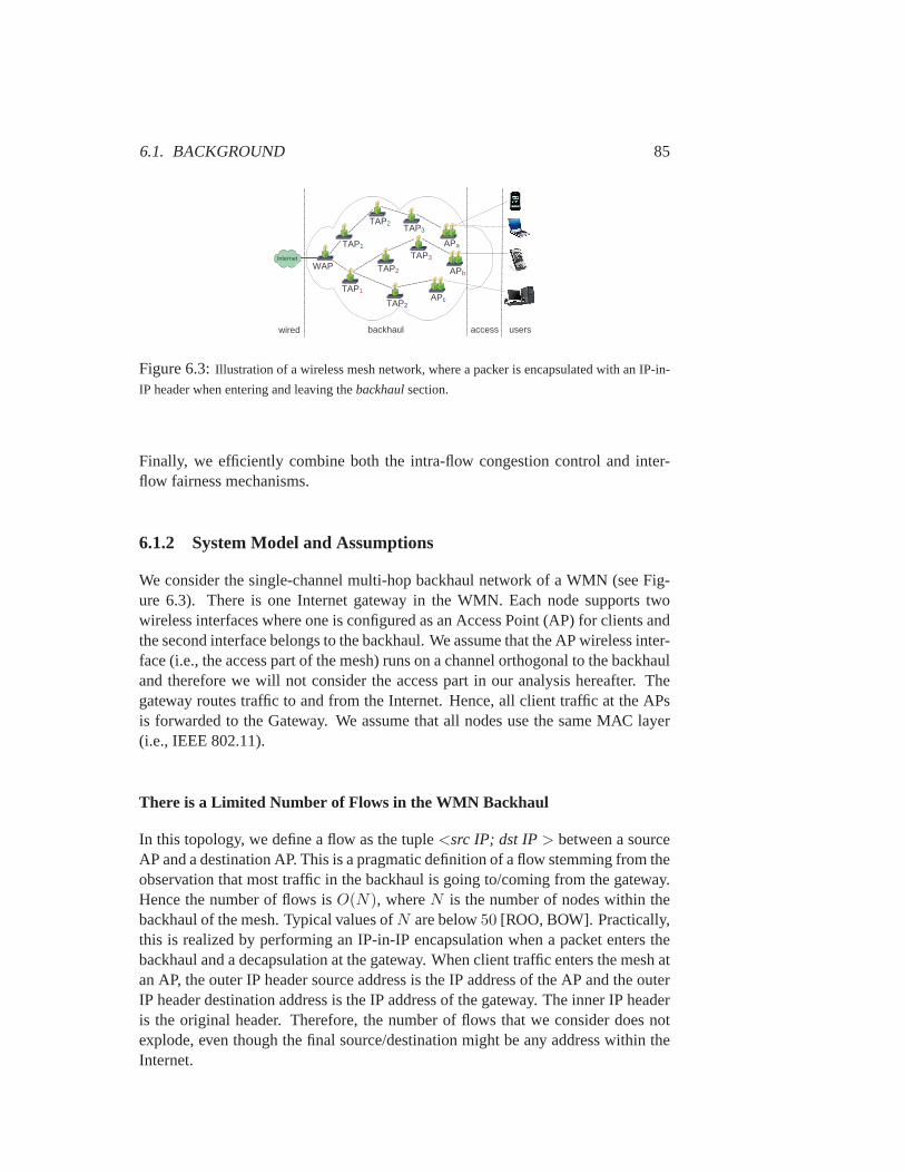
6.1. BACKGROUND 85
Internet
backhaul users
ä
LNK/ACT
INTERNET
accesswired
WAP
ä
LNK/ACT
INTERNET
ä
LNK/ACT
INTERNET
ä
LNK/ACT
INTERNET
ä
LNK/ACT
INTERNET
ä
LNK/ACT
INTERNET
ä
LNK/ACT
INTERNET
ä
LNK/ACT
INTERNET
ä
LNK/ACT
INTERNET
ä
LNK/ACT
INTERNET
ä
LNK/ACT
INTERNET
ä
LNK/ACT
INTERNET
ä
LNK/ACT
INTERNET
ä
LNK/ACT
INTERNET
APcTAP2
APa
APb
TAP1
TAP2TAP3
TAP2
TAP3
TAP1
Figure 6.3:Illustration of a wireless mesh network, where a packer is encapsulated with an IP-in-
IP header when entering and leaving thebackhaulsection.
Finally, we efficiently combine both the intra-flow congestion control and inter-flow fairness mechanisms.
6.1.2 System Model and Assumptions
We consider the single-channel multi-hop backhaul network of a WMN (see Fig-ure 6.3). There is one Internet gateway in the WMN. Each node supportstwowireless interfaces where one is configured as an Access Point (AP) for clients andthe second interface belongs to the backhaul. We assume that the AP wireless inter-face (i.e., the access part of the mesh) runs on a channel orthogonal tothe backhauland therefore we will not consider the access part in our analysis hereafter. Thegateway routes traffic to and from the Internet. Hence, all client traffic at the APsis forwarded to the Gateway. We assume that all nodes use the same MAC layer(i.e., IEEE 802.11).
There is a Limited Number of Flows in the WMN Backhaul
In this topology, we define a flow as the tuple<src IP; dst IP> between a sourceAP and a destination AP. This is a pragmatic definition of a flow stemming from theobservation that most traffic in the backhaul is going to/coming from the gateway.Hence the number of flows isO(N), whereN is the number of nodes within thebackhaul of the mesh. Typical values ofN are below50 [ROO, BOW]. Practically,this is realized by performing an IP-in-IP encapsulation when a packet enters thebackhaul and a decapsulation at the gateway. When client traffic entersthe mesh atan AP, the outer IP header source address is the IP address of the AP and the outerIP header destination address is the IP address of the gateway. The inner IP headeris the original header. Therefore, the number of flows that we considerdoes notexplode, even though the final source/destination might be any address within theInternet.
86 CHAPTER 6. JOINT CONGESTION-CONTROL AND FAIRNESS
Rate of a Flow and Capacity Region
AssumingF flows in the backhaul indexed from1 to F , we denote the rate of aflow j, j ∈ {1, . . . , F} by xj . Additionally, we denote the flow rate vector by
~x = [x1 x2 . . . xF ].
Observe that, given our definition of flows in the previous paragraph,xj is the rateachieved above the MAC layer.
Finally, we denote byΛ the network capacity region, which is the set of allachievable rate vectors~x.
Intra-Flow and Inter-Flow Performance Issues
Performance problems with decentralized CSMA/CA protocols, e.g. IEEE 802.11,in wireless multi-hop networks can be divided into two categories:
• Intra-flow Congestion Problem: Already with a single flow, network in-stability can occur. The queues of the relay nodes build up, reducing thethroughput and increasing end-to-end delays. Indeed, we showed inChap-ter 3 and 5 that the intra-flow congestion is due to the inefficiency of de-centralized CSMA/CA protocols to form a smooth flow of packets whentransporting the traffic hop-by-hop through the network.
• Inter-flow Fairness Problem: With two or more flows, interference betweenflows can lead to serious unfairness and starvation problems if no counter-policy is applied. This occurs with TCP in simple topologies where one ormore1-hop flows compete with one largerK-hop flow (K ≥ 2) [GMSK09].In Figure 6.2, our experiments show that unfairness and starvation are notlimited to TCP and that they also occur with UDP. In these experiments,a 1-hop flow competes with a2-hop (or3-hop) flow. We observe that fairqueuing is clearly needed to achieve fairness, but is not sufficient by itself.
Tradeoff between Fairness and Throughput
There is a tradeoff between (i) maximizing the total throughput and (ii) fairly shar-ing the capacity among competing flows. This tradeoff is intimately related to themaximization of a utility functionu(·) of the flow rates [ES05].
For instance, Remember thatxj is the rate of flowj: maximizing
uthr(~x) =F∑
j=1
xj (6.1)
yields the maximum total throughput but completely ignores fairness. A utilityfunction effectively balancing throughput and fairness is
uprop(~x) =
F∏
j=1
xj . (6.2)
6.1. BACKGROUND 87
This utility function achievesproportional fairness[KMT98], because maximizing(6.2) is exactly the same as maximizing
u(~x) =F∑
j=1
log(xj).
In the remainder of the chapter, we will consider the utility functions (6.1) and(6.2). The reader interested in further extensions of proportional fairness can con-sult [MW00].
Then, for a given utility functionu(·) (i.e., either (6.1) or (6.2)), solving theoptimization problem
max~x∈Λ
u(~x) (6.3)
finds a rate allocation vector~x that maximizes the utility function and satisfies theparticular fairness implicitly embedded by the definition ofu(·). Note that directlysolving the maximization problem (6.3) in one step would imply the knowledge ofthe capacity regionΛ. However, the capacity region is, in practice, time-varyingand challenging to measure [SSGG09] and therefore there is a real needfor dy-namic mechanisms such as the one that we propose in this chapter.
6.1.3 Related Work
As explained in Section 6.1, the serious unfairness and starvation problemsthatwe observe in Figure 6.2 find their origins in both: (i) a queuing problem and(ii)a MAC problem. The queuing problem has been thoroughly studied for wirednetworks [DKS89, PG93]: flow-based scheduling with Weighted Fair Queuing(WFQ) efficiently provides fairness. However, WFQ alone is not sufficient forwireless multi-hop networks [GSK04] because the MAC layer plays a criticalrole.
In the previous chapters, we already discussed the recent analytical work onthroughput optimal schemes [YST08, CKLS08, PYC08, YPC08, GLS07, SSR09].Their goal is to achieve any rate in the capacity region by using variants of theMaxWeight scheduling algorithm [PYC08, SSR09]. It is important to point out thatthese approaches rely on three fundamental conditions: (i) the set of active flowsin the network must be static and no flow can appear (or leave) [vdVBS09], (ii) allsources should know a priori the capacity region and (iii) no source cantransmit ata rate above capacity. Our work fundamentally differs because we do not assumethat the sources know the capacity region nor that they rate-limit themselves at thecapacity of the network. Our mechanisms do not rely on any assumption about thesource behavior and provide both congestion control and fairness in adistributedmanner.
Interestingly, in [ES05] Eryilmaz et al. show for single-hop cellular networksthat a combination of queue-length-based scheduling and congestion control leadsto a fair resource allocation. Our work differs as we consider multi-hop scenariosthat require distributed solutions because there exists no base stations thatcan actas a central scheduler.
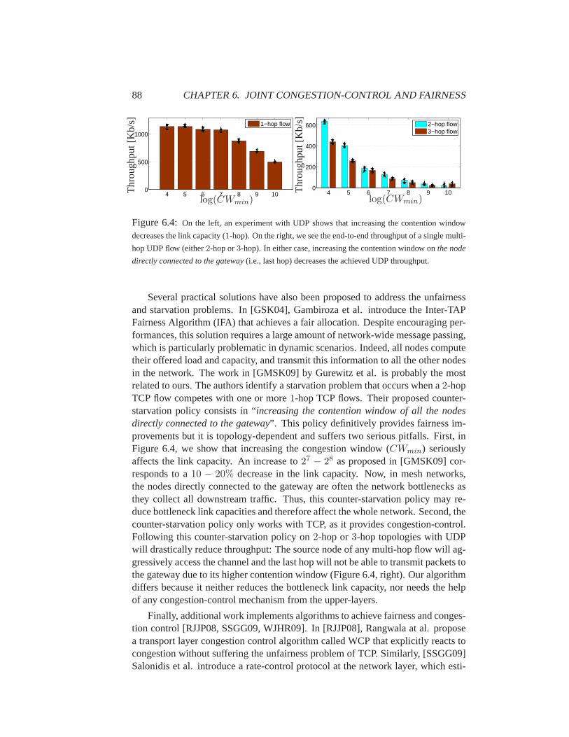
88 CHAPTER 6. JOINT CONGESTION-CONTROL AND FAIRNESS
4 5 6 7 8 9 100
500
1000
1−hop flowT
hrou
ghpu
t[K
b/s]
log(CWmin)4 5 6 7 8 9 10
0
200
400
600
2−hop flow3−hop flow
Thr
ough
put[
Kb/
s]
log(CWmin)
Figure 6.4:On the left, an experiment with UDP shows that increasing the contention window
decreases the link capacity (1-hop). On the right, we see the end-to-end throughput of a single multi-
hop UDP flow (either2-hop or3-hop). In either case, increasing the contention window onthe node
directly connected to the gateway(i.e., last hop) decreases the achieved UDP throughput.
Several practical solutions have also been proposed to address the unfairnessand starvation problems. In [GSK04], Gambiroza et al. introduce the Inter-TAPFairness Algorithm (IFA) that achieves a fair allocation. Despite encouraging per-formances, this solution requires a large amount of network-wide messagepassing,which is particularly problematic in dynamic scenarios. Indeed, all nodes computetheir offered load and capacity, and transmit this information to all the other nodesin the network. The work in [GMSK09] by Gurewitz et al. is probably the mostrelated to ours. The authors identify a starvation problem that occurs when a2-hopTCP flow competes with one or more1-hop TCP flows. Their proposed counter-starvation policy consists in “increasing the contention window of all the nodesdirectly connected to the gateway”. This policy definitively provides fairness im-provements but it is topology-dependent and suffers two serious pitfalls. First, inFigure 6.4, we show that increasing the congestion window (CWmin) seriouslyaffects the link capacity. An increase to27 − 28 as proposed in [GMSK09] cor-responds to a10 − 20% decrease in the link capacity. Now, in mesh networks,the nodes directly connected to the gateway are often the network bottlenecks asthey collect all downstream traffic. Thus, this counter-starvation policy may re-duce bottleneck link capacities and therefore affect the whole network. Second, thecounter-starvation policy only works with TCP, as it provides congestion-control.Following this counter-starvation policy on2-hop or3-hop topologies with UDPwill drastically reduce throughput: The source node of any multi-hop flow willag-gressively access the channel and the last hop will not be able to transmitpackets tothe gateway due to its higher contention window (Figure 6.4, right). Our algorithmdiffers because it neither reduces the bottleneck link capacity, nor needs the helpof any congestion-control mechanism from the upper-layers.
Finally, additional work implements algorithms to achieve fairness and conges-tion control [RJJP08, SSGG09, WJHR09]. In [RJJP08], Rangwala at al. proposea transport layer congestion control algorithm called WCP that explicitly reacts tocongestion without suffering the unfairness problem of TCP. Similarly, [SSGG09]Salonidis et al. introduce a rate-control protocol at the network layer, which esti-

6.2. INTRA-FLOW CONGESTION CONTROL 89
...
Queueq1i
Queueq2i
QueueqFi
ρ1i
ρ2i
ρFi
IP MAC queueRR scheduler
Figure 6.5:Congestion control mechanism running at nodei, with each flowj having its dedicated
queue and rate limiterρji (limiting the link rate). A round-robin (RR) scheduler connects the rate
limiters to the MAC (interface) queue.
mates the network capacity and adapts the transmission rate accordingly to avoidcongestion. Nevertheless, both protocols build upon an end-to-end methodology,better suited for a static network than a dynamic one. Hop-by-hop approacheshave the potential to provide better performance [YS07]. Both DiffQ [WJHR09]and EZ-flow (see Chapter 5) are hop-by-hop protocols that performcongestioncontrol at the MAC layer by using different values for the contention windowparameter (CWmin). Despite good performance, DiffQ and EZ-flow abuse therole of theCWmin, originally meant to deal with contention and not congestion.This abuse leads to antagonist goals between congestion (avoiding queuebuild-up) and contention (avoiding collisions) whenever a part of the network suffersfrom both. Indeed, the congestion-control mechanism tends to decrease CWmin
in order to to flush the queue faster, whereas the contention-control mechanismtends to increaseCWmin to avoid collisions. Congestion-control must be decou-pled from contention-control at the MAC layer. Similarly to the methodology ofEZ-flow, discussed in previous chapter, our network-layer hop-by-hop congestion-control algorithm works without message passing, but it significantly differs fromthe scheme of the previous chapter, because there are no interactions withthe MAClayer. Moreover, here we also consider the notion of fairness throughan inter-flowmechanism.
6.2 Intra-Flow Congestion Control
For a single multi-hop flow, the goal of intra-flow congestion control is to createa smooth packet flow with low end-to-end delays and high throughput. We usea hop-by-hop approach where the link rates of the source and its relay nodes areadapted to maintain a small (but non-zero) number of packets in the relay queues.Obviously, the last node just before the destination is not rate limited.
In this chapter, we design a novel layer2.5 protocol performing per-flow queu-ing at each nodei. As depicted in Figure 6.5, each queue is attached to arate
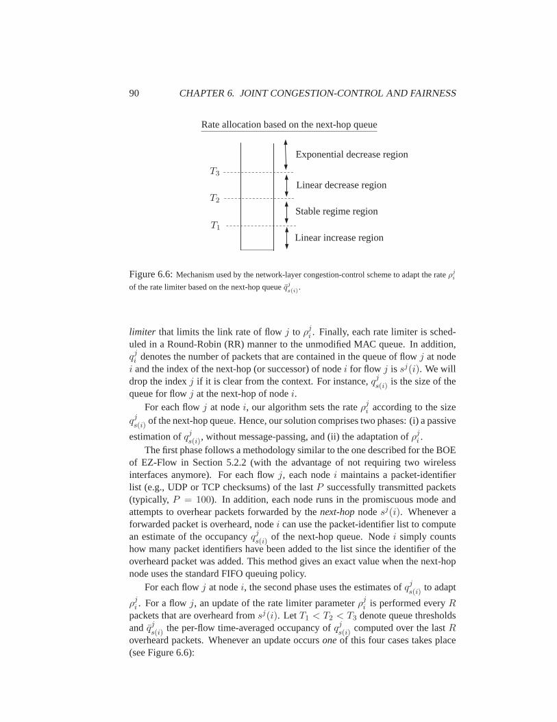
90 CHAPTER 6. JOINT CONGESTION-CONTROL AND FAIRNESS
T3
T2
T1
Rate allocation based on the next-hop queue
Exponential decrease region
Linear decrease region
Stable regime region
Linear increase region
Figure 6.6:Mechanism used by the network-layer congestion-control scheme to adapt the rateρjiof the rate limiter based on the next-hop queueqj
s(i).
limiter that limits the link rate of flowj to ρji . Finally, each rate limiter is sched-uled in a Round-Robin (RR) manner to the unmodified MAC queue. In addition,qji denotes the number of packets that are contained in the queue of flowj at nodei and the index of the next-hop (or successor) of nodei for flow j is sj(i). We willdrop the indexj if it is clear from the context. For instance,qjs(i) is the size of thequeue for flowj at the next-hop of nodei.
For each flowj at nodei, our algorithm sets the rateρji according to the sizeqjs(i) of the next-hop queue. Hence, our solution comprises two phases: (i) a passive
estimation ofqjs(i), without message-passing, and (ii) the adaptation ofρji .The first phase follows a methodology similar to the one described for the BOE
of EZ-Flow in Section 5.2.2 (with the advantage of not requiring two wirelessinterfaces anymore). For each flowj, each nodei maintains a packet-identifierlist (e.g., UDP or TCP checksums) of the lastP successfully transmitted packets(typically, P = 100). In addition, each node runs in the promiscuous mode andattempts to overhear packets forwarded by thenext-hopnodesj(i). Whenever aforwarded packet is overheard, nodei can use the packet-identifier list to computean estimate of the occupancyqjs(i) of the next-hop queue. Nodei simply countshow many packet identifiers have been added to the list since the identifier oftheoverheard packet was added. This method gives an exact value whenthe next-hopnode uses the standard FIFO queuing policy.
For each flowj at nodei, the second phase uses the estimates ofqjs(i) to adapt
ρji . For a flowj, an update of the rate limiter parameterρji is performed everyRpackets that are overheard fromsj(i). Let T1 < T2 < T3 denote queue thresholdsand qjs(i) the per-flow time-averaged occupancy ofqjs(i) computed over the lastRoverheard packets. Whenever an update occursoneof this four cases takes place(see Figure 6.6):
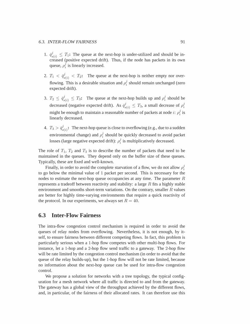
6.3. INTER-FLOW FAIRNESS 91
1. qjs(i) ≤ T1: The queue at the next-hop is under-utilized and should be in-creased (positive expected drift). Thus, if the node has packets in its ownqueue,ρji is linearly increased.
2. T1 < qjs(i) < T2: The queue at the next-hop is neither empty nor over-
flowing. This is a desirable situation andρji should remain unchanged (zeroexpected drift).
3. T2 ≤ qjs(i) ≤ T3: The queue at the next-hop builds up andρji should be
decreased (negative expected drift). Asqjs(i) ≤ T3, a small decrease ofρjimight be enough to maintain a reasonable number of packets at nodei: ρji islinearly decreased.
4. T3 > qjs(i): The next-hop queue is close to overflowing (e.g., due to a sudden
environmental change) andρji should be quickly decreased to avoid packetlosses (large negative expected drift):ρji is multiplicatively decreased.
The role ofT1, T2 andT3 is to describe the number of packets that need to bemaintained in the queues. They depend only on the buffer size of these queues.Typically, these are fixed and well-known.
Finally, in order to avoid the complete starvation of a flow, we do not allowρjito go below the minimal value of1 packet per second. This is necessary for thenodes to estimate the next-hop queue occupancies at any time. The parameterRrepresents a tradeoff between reactivity and stability: a largeR fits a highly stableenvironment and smooths short-term variations. On the contrary, smallerR valuesare better for highly time-varying environments that require a quick reactivity ofthe protocol. In our experiments, we always setR = 40.
6.3 Inter-Flow Fairness
The intra-flow congestion control mechanism is required in order to avoid thequeues of relay nodes from overflowing. Nevertheless, it is not enough, by it-self, to ensure fairness between different competing flows. In fact, thisproblem isparticularly serious when a1-hop flow competes with other multi-hop flows. Forinstance, let a1-hop and a2-hop flow send traffic to a gateway. The2-hop flowwill be rate limited by the congestion control mechanism (in order to avoid that thequeue of the relay builds-up), but the1-hop flow will not be rate limited, becauseno information about the next-hop queue can be used for intra-flow congestioncontrol.
We propose a solution for networks with a tree topology, the typical config-uration for a mesh network where all traffic is directed to and from the gateway.The gateway has a global view of the throughput achieved by the different flows,and, in particular, of the fairness of their allocated rates. It can therefore use this
92 CHAPTER 6. JOINT CONGESTION-CONTROL AND FAIRNESS
information to set the rate of the rate limiters of its directly connected neighbors.A network with multiple gateways is a straightforward extension. Indeed, the mul-tiple gateways can use their wired links to exchange information, thus making theproblem similar to the case of a macro-gateway making the scheduling decisionsfor the whole network.
We believe that it is relevant to consider this fairness problem separately,in asingle-hop scenario. Indeed, any rate adaptation on the last hop induced by a fair-ness enforcement policy will propagate along the mesh using the intra-flow con-gestion control mechanism, as discussed in Section 6.4. The experimental resultsin Section 6.5 confirm this behavior.
6.3.1 Model Description
We focus on a single-hop scenario, whereF flows j (j ∈ {1, . . . , F}) send trafficto the gateway. We assume that the capacity regionΛ(n) is unknown, but for thepurpose of the analysis, also time-constant (Λ(n) = Λ) and convex. In these set-tings, the fairness problem can be modeled as the utility maximization of a slotted-time system. A time slot corresponds to the fixed duration of a rate limiting (ratelimiter) assignment.
We adapt the notation of Sections 6.1.2 and 6.2. We drop the node indexi andextend the notation to consider the time-slotted behavior.
• Service rate: ~x(n) ∈ RF , wherexj(n) is the amount of traffic received at
the gateway from flowj during time slotn.
• Limiting rate : ~ρ(n) ∈ RF , whereρj(n) is the maximum amount of traffic
set by the gateway for flowj during time slotn.
• Capacity region: Λ(n), which is the set of all the achievable~x(n) by thesystem
• Utility function : We consider a concave, continuously differentiable andstrictly increasing utility functionu : RF → R. We denoteu(n) = u(~x(n))the utility achieved at slotn that can be computed by the gateway.
The achieved throughput vector~x(n) obviously depends on the value of therate limiters when~ρ(n) ∈ Λ(n). Indeed, we have
~x(n) = ~ρ(n) (6.4)
when~ρ(n) ∈ Λ(n). Otherwise, we can only write that
~x(n) ∈ ∂Λ(n),
where∂Λ(n) is the boundary of the capacity regionΛ(n). This constraint meansthat the gateway has full control of the service rate achieved by each flow when~ρ(n) ∈ Λ(n). However, it loses this control, when going out of this region.
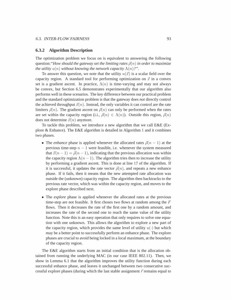
6.3. INTER-FLOW FAIRNESS 93
6.3.2 Algorithm Description
The optimization problem we focus on is equivalent to answering the followingquestion:“How should the gateway set the limiting rates~ρ(n) in order to maximizethe utilityu(n) without knowing the network capacityΛ(n)?” .
To answer this question, we note that the utilityu(~x) is a scalar field over thecapacity region. A standard tool for performing optimization on~x in a convexset is a gradient ascent. In practice,Λ(n) is time-varying and may not alwaysbe convex, but Section 6.5 demonstrates experimentally that our algorithm alsoperforms well in these scenarios. The key difference between our practical problemand the standard optimization problem is that the gateway doesnotdirectly controlthe achieved throughput~x(n). Instead, the only variables it can control are the ratelimiters ~ρ(n). The gradient ascent on~ρ(n) can only be performed when the ratesare set within the capacity region (i.i.,~ρ(n) ∈ Λ(n)). Outside this region,~ρ(n)does not determine~x(n) anymore.
To tackle this problem, we introduce a new algorithm that we call E&E (Ex-plore & Enhance). The E&E algorithm is detailed in Algorithm1 and it combinestwo phases.
• The enhancephase is applied whenever the allocated rates~ρ(n − 1) at theprevious time-stepn − 1 were feasible, i.e. whenever the system measuredthat~x(n− 1) = ~ρ(n− 1), indicating that the previous allocation was withinthe capacity regionΛ(n− 1). The algorithm tries then to increase the utilityby performing a gradient ascent. This is done at line17 of the algorithm. Ifit is successful, it updates the rate vector~ρ(n), and repeats a new enhancephase. If it fails, then it means that the new attempted rate allocation wasoutside the (unknown) capacity region. The algorithm then backtracks to theprevious rate vector, which was within the capacity region, and moves to theexplore phase described next.
• The explorephase is applied whenever the allocated rates at the previoustime-step are not feasible. It first choses two flows at random among theFflows. Then it decreases the rate of the first one by a random amount, andincreases the rate of the second one to reach the same value of the utilityfunction. Note this is an easy operation that only requires to solve one equa-tion with one unknown. This allows the algorithm to explore a new part ofthe capacity region, which provides the same level of utilityu(·) but whichmay be a better point to successfully perform an enhance phase. The explorephases are crucial to avoid being locked in a local maximum, at the boundaryof the capacity region.
The E&E algorithm starts from an initial condition that is the allocation ob-tained from running the underlying MAC (in our case IEEE 802.11). Then, weshow in Lemma 6.1 that the algorithm improves the utility function during eachsuccessful enhance phase, and leaves it unchanged between two consecutive suc-cessful explore phases (during which the last stable assignment~r remains equal to
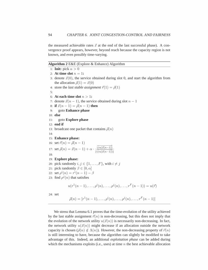
94 CHAPTER 6. JOINT CONGESTION-CONTROL AND FAIRNESS
the measured achievable rates~x at the end of the last successful phase). A con-vergence proof appears, however, beyond reach because the capacity region is notknown, and even possibly time-varying.
Algorithm 2 E&E (Explore & Enhance) Algorithm1: Init: pick α > 02: At time slot n = 1:3: denote~x(0), the service obtained during slot 0, and start the algorithm from
the allocation~ρ(1) = ~x(0)4: store thelast stable assignment~r(1) = ~ρ(1)5:
6: At each time slotn > 1:7: denote~x(n− 1), the service obtained during slotn− 18: if ~x(n− 1) = ~ρ(n− 1) then9: gotoEnhance phase
10: else11: gotoExplore phase12: end if13: broadcast one packet that contains~ρ(n)14:
15: Enhance phase:16: set~r(n) = ~ρ(n− 1)
17: set~ρ(n) = ~x(n− 1) + α ·−−−−−−−−−→▽u(~x(n−1))
‖−−−−−−−−−→▽u(~x(n−1))‖
18:
19: Explore phase:20: pick randomlyi, j ∈ {1, . . . , F}, with i 6= j21: pick randomlyβ ∈ [0, α]22: setρi(n) = ri(n− 1)− β23: find ρj(n) that satisfies
u(r1(n− 1), . . . , ρi(n), . . . , ρj(n), . . . , rF (n− 1)) = u(~r)
24: set~ρ(n) = [r1(n− 1), . . . , ρi(n), . . . , ρj(n), . . . , rF (n− 1)]
We stress that Lemma 6.1 proves that the time-evolution of the utility achievedby the last stable assignment~r(n) is non-decreasing, but this does not imply thatthe evolution of the network utilityu(~x(n)) is necessarily non-decreasing. In fact,the network utilityu(~x(n)) might decrease if an allocation outside the networkcapacity is chosen (~ρ(n) /∈ Λ(n)). However, the non-decreasing property of~r(n)is still interesting to have, because the algorithm can slightly be modified to takeadvantage of this. Indeed, an additionalexploitation phasecan be added duringwhich the mechanisms exploits (i.e., uses) at timen the best achievable allocation
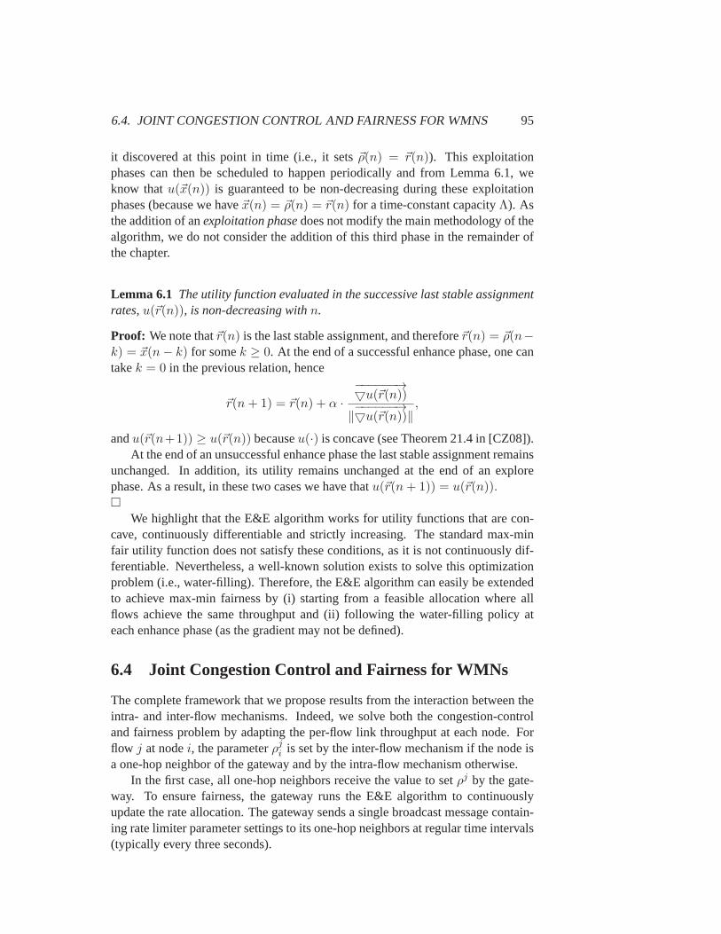
6.4. JOINT CONGESTION CONTROL AND FAIRNESS FOR WMNS 95
it discovered at this point in time (i.e., it sets~ρ(n) = ~r(n)). This exploitationphases can then be scheduled to happen periodically and from Lemma 6.1, weknow thatu(~x(n)) is guaranteed to be non-decreasing during these exploitationphases (because we have~x(n) = ~ρ(n) = ~r(n) for a time-constant capacityΛ). Asthe addition of anexploitation phasedoes not modify the main methodology of thealgorithm, we do not consider the addition of this third phase in the remainder ofthe chapter.
Lemma 6.1 The utility function evaluated in the successive last stable assignmentrates,u(~r(n)), is non-decreasing withn.
Proof: We note that~r(n) is the last stable assignment, and therefore~r(n) = ~ρ(n−k) = ~x(n− k) for somek ≥ 0. At the end of a successful enhance phase, one cantakek = 0 in the previous relation, hence
~r(n+ 1) = ~r(n) + α ·
−−−−−−→▽u(~r(n))
‖−−−−−−→▽u(~r(n))‖
,
andu(~r(n+1)) ≥ u(~r(n)) becauseu(·) is concave (see Theorem 21.4 in [CZ08]).At the end of an unsuccessful enhance phase the last stable assignment remains
unchanged. In addition, its utility remains unchanged at the end of an explorephase. As a result, in these two cases we have thatu(~r(n+ 1)) = u(~r(n)).�
We highlight that the E&E algorithm works for utility functions that are con-cave, continuously differentiable and strictly increasing. The standard max-minfair utility function does not satisfy these conditions, as it is not continuouslydif-ferentiable. Nevertheless, a well-known solution exists to solve this optimizationproblem (i.e., water-filling). Therefore, the E&E algorithm can easily be extendedto achieve max-min fairness by (i) starting from a feasible allocation where allflows achieve the same throughput and (ii) following the water-filling policy ateach enhance phase (as the gradient may not be defined).
6.4 Joint Congestion Control and Fairness for WMNs
The complete framework that we propose results from the interaction between theintra- and inter-flow mechanisms. Indeed, we solve both the congestion-controland fairness problem by adapting the per-flow link throughput at each node. Forflow j at nodei, the parameterρji is set by the inter-flow mechanism if the node isa one-hop neighbor of the gateway and by the intra-flow mechanism otherwise.
In the first case, all one-hop neighbors receive the value to setρj by the gate-way. To ensure fairness, the gateway runs the E&E algorithm to continuouslyupdate the rate allocation. The gateway sends a single broadcast messagecontain-ing rate limiter parameter settings to its one-hop neighbors at regular time intervals(typically every three seconds).
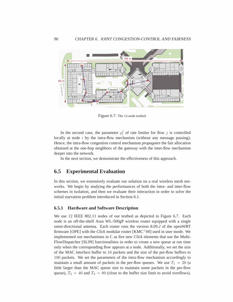
96 CHAPTER 6. JOINT CONGESTION-CONTROL AND FAIRNESS
66 m
186 m
11
10
9
5
4
1
3
2
7
0
6
Figure 6.7:The12-node testbed.
In the second case, the parameterρji of rate limiter for flow j is controlledlocally at nodei by the intra-flow mechanism (without any message passing).Hence, the intra-flow congestion control mechanismpropagatesthe fair allocationobtained at the one-hop neighbors of the gateway with the inter-flow mechanismdeeper into the network.
In the next section, we demonstrate the effectiveness of this approach.
6.5 Experimental Evaluation
In this section, we extensively evaluate our solution on a real wireless meshnet-works. We begin by studying the performances of both the intra- and inter-flowschemes in isolation, and then we evaluate their interaction in order to solve theinitial starvation problem introduced in Section 6.1.
6.5.1 Hardware and Software Description
We use12 IEEE 802.11 nodes of our testbed as depicted in Figure 6.7. Eachnode is an off-the-shelf Asus WL-500gP wireless router equipped with asingleomni-directional antenna. Each router runs the version8.09.2of the openWRTfirmware [OPE] with theClick modular router [KMC+00] used in user mode. Weimplemented our mechanisms in C as five newClick elements that use the Multi-FlowDispatcher [SL09] functionalities in order to create a new queue at run timeonly when the corresponding flow appears at a node. Additionally, we set the sizeof the MAC interface buffer to10 packets and the size of the per-flow buffers to100 packets. We set the parameters of the intra-flow mechanism accordingly tomaintain a small amount of packets in the per-flow queues. We useT1 = 20 (alittle larger than the MAC queue size to maintain some packets in the per-flowqueue),T2 = 40 andT3 = 80 (close to the buffer size limit to avoid overflows).
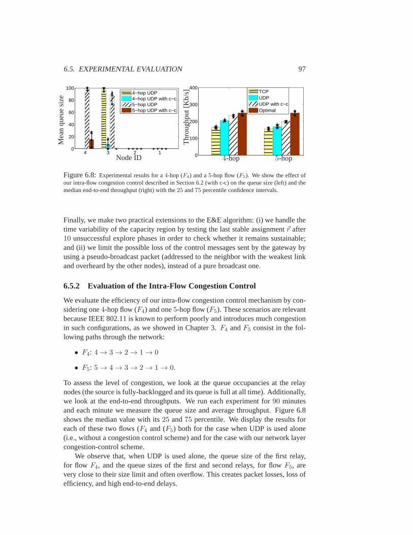
6.5. EXPERIMENTAL EVALUATION 97
4 3 2 10
20
40
60
80
100
4−hop UDP4−hop UDP with c−c5−hop UDP5−hop UDP with c−c
Mea
nqu
eue
size
Node ID 0
100
200
300
400
TCPUDPUDP with c−cOptimal
4-hop 5-hop
Thr
ough
put[
Kb/
s]
Figure 6.8:Experimental results for a4-hop (F4) and a5-hop flow (F5). We show the effect ofour intra-flow congestion control described in Section 6.2 (with c-c) on the queue size (left) and themedian end-to-end throughput (right) with the25 and75 percentile confidence intervals.
Finally, we make two practical extensions to the E&E algorithm: (i) we handle thetime variability of the capacity region by testing the last stable assignment~r after10 unsuccessful explore phases in order to check whether it remains sustainable;and (ii) we limit the possible loss of the control messages sent by the gateway byusing a pseudo-broadcast packet (addressed to the neighbor with theweakest linkand overheard by the other nodes), instead of a pure broadcast one.
6.5.2 Evaluation of the Intra-Flow Congestion Control
We evaluate the efficiency of our intra-flow congestion control mechanismby con-sidering one4-hop flow (F4) and one5-hop flow (F5). These scenarios are relevantbecause IEEE 802.11 is known to perform poorly and introduces much congestionin such configurations, as we showed in Chapter 3.F4 andF5 consist in the fol-lowing paths through the network:
• F4: 4→ 3→ 2→ 1→ 0
• F5: 5→ 4→ 3→ 2→ 1→ 0.
To assess the level of congestion, we look at the queue occupancies atthe relaynodes (the source is fully-backlogged and its queue is full at all time). Additionally,we look at the end-to-end throughputs. We run each experiment for90 minutesand each minute we measure the queue size and average throughput. Figure 6.8shows the median value with its25 and75 percentile. We display the results foreach of these two flows (F4 and (F5) both for the case when UDP is used alone(i.e., without a congestion control scheme) and for the case with our network layercongestion-control scheme.
We observe that, when UDP is used alone, the queue size of the first relay,for flow F4, and the queue sizes of the first and second relays, for flowF5, arevery close to their size limit and often overflow. This creates packet losses, loss ofefficiency, and high end-to-end delays.
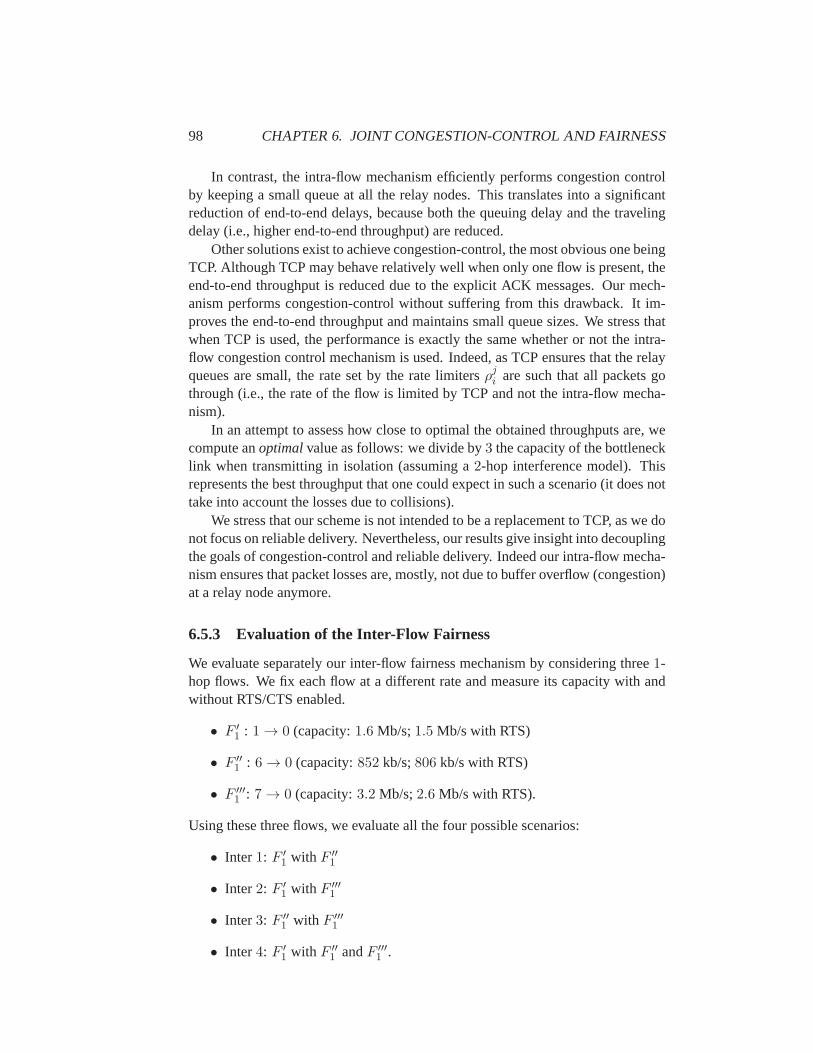
98 CHAPTER 6. JOINT CONGESTION-CONTROL AND FAIRNESS
In contrast, the intra-flow mechanism efficiently performs congestion controlby keeping a small queue at all the relay nodes. This translates into a significantreduction of end-to-end delays, because both the queuing delay and thetravelingdelay (i.e., higher end-to-end throughput) are reduced.
Other solutions exist to achieve congestion-control, the most obvious one beingTCP. Although TCP may behave relatively well when only one flow is present, theend-to-end throughput is reduced due to the explicit ACK messages. Ourmech-anism performs congestion-control without suffering from this drawback. It im-proves the end-to-end throughput and maintains small queue sizes. We stress thatwhen TCP is used, the performance is exactly the same whether or not the intra-flow congestion control mechanism is used. Indeed, as TCP ensures that the relayqueues are small, the rate set by the rate limitersρji are such that all packets gothrough (i.e., the rate of the flow is limited by TCP and not the intra-flow mecha-nism).
In an attempt to assess how close to optimal the obtained throughputs are, wecompute anoptimalvalue as follows: we divide by3 the capacity of the bottlenecklink when transmitting in isolation (assuming a2-hop interference model). Thisrepresents the best throughput that one could expect in such a scenario (it does nottake into account the losses due to collisions).
We stress that our scheme is not intended to be a replacement to TCP, as we donot focus on reliable delivery. Nevertheless, our results give insightinto decouplingthe goals of congestion-control and reliable delivery. Indeed our intra-flow mecha-nism ensures that packet losses are, mostly, not due to buffer overflow (congestion)at a relay node anymore.
6.5.3 Evaluation of the Inter-Flow Fairness
We evaluate separately our inter-flow fairness mechanism by consideringthree1-hop flows. We fix each flow at a different rate and measure its capacity withandwithout RTS/CTS enabled.
• F ′1 : 1→ 0 (capacity:1.6 Mb/s;1.5 Mb/s with RTS)
• F ′′1 : 6→ 0 (capacity:852 kb/s;806 kb/s with RTS)
• F ′′′1 : 7→ 0 (capacity:3.2 Mb/s;2.6 Mb/s with RTS).
Using these three flows, we evaluate all the four possible scenarios:
• Inter1: F ′1 with F ′′
1
• Inter2: F ′1 with F ′′′
1
• Inter3: F ′′1 with F ′′′
1
• Inter4: F ′1 with F ′′
1 andF ′′′1 .
6.5. EXPERIMENTAL EVALUATION 99
Proportional Fairness Throughput Maximization
Inter 1 Inter 2 Inter 3 Inter 40
0.5
1
without EEwith EEbenchmark
Nor
mal
ized
utili
ty
ScenarioInter 1 Inter 2 Inter 3 Inter 4
0
0.5
1
without EEwith EEbenchmark
Nor
mal
ized
utili
ty
Scenario
F1’ F1’’ F1’’ F1’’’ F1’’ F1’’’ F1’ F1’’ F1’’’0
0.5
1
1.5
2
without EEwith EEbenchmark
Inter 4Inter 2Inter 1 Inter 3
Thr
ough
put[
Mb/
s]
F1’ F1’’ F1’ F1’’’ F1’’ F1’’’ F1’ F1’’ F1’’’0
0.5
1
1.5
2
2.5
3
3.5
without EEwith EEbenchmark
Inter 1 Inter 2 Inter 3 Inter 4
Thr
ough
put[
Mb/
s]
Figure 6.9: Illustration of the normalized utility and throughput achieved with and without ourE&E mechanism for the four inter-flow scenarios. We show its performance for both utilities: pro-portional fairness (left) and throughput maximization (right).
As the sources fromF ′′1 andF ′′′
1 are hidden from each other, we turn on theRTS/CTS mechanism in the scenarios Inter2 and Inter4, otherwise we turn it off.We test the efficiency of our algorithm for both the proportional fairness(Eq. 6.2)and max-throughput (Eq. 6.1) utility functions. We present our results in Figure 6.9by showing both the achieved utility (normalized with respect to the theoreticalupper-bound) and the per-flow throughput obtained for each scenario. We obtainthe theoretical upper-bound by assuming an idealized MAC that prevents any colli-sion from happening between flows. In such a case, the proportionally fair optimalallocation for each flowj isCj/F , whereCj is the flow capacity when transmittingin isolation andF is the number of flows transmitting concurrently. Nevertheless,this upper-bound allocation is not necessarily achievable by IEEE 802.11due tocollisions (e.g., in the case of hidden nodes). Therefore, in order to allowfor a faircomparison of our algorithm, we measure abenchmarkallocation that is obtainedby setting the source traffic rates at the rate given by the upper-bound allocation.We stress that our benchmark point is not necessarily the optimal point in thecaseof collisions (as the sources need to send at a lower rate due to collisions).How-ever as the exact capacity region is unknown, the optimal point is also unknown.Thus our benchmark is a good comparison point in addition to the performancesachieved by IEEE 802.11 without the E&E algorithm. Our results show that theinter-flow algorithm improves the performances in all scenarios (comparedto both
100 CHAPTER 6. JOINT CONGESTION-CONTROL AND FAIRNESS
IEEE 802.11 and the benchmark). Furthermore in the case of scenarios withoutcollision, our algorithm reaches the theoretical optimal fair allocation.
For the case of throughput maximization, the optimal point is trivially obtainedby giving all the throughput to the flow with the better link quality and by starvingthe other flows. Nevertheless, the policy of E&E is to never completely starve aflow so that the gateway can maintain a global view of all the flows existing inthe network (i.e., it is impossible to detect whether a flow exists or not if it iscompletely starved by a rate limiter). Despite this difference, in the case withoutcollision (Inter1 and Inter3), the E&E algorithm reaches a point that is very closeto the optimal allocation, even though it does not starve the flow with the weakestlink capacity.
In the case of hidden nodes (the scenarios Inter2 and Inter4), the E&E algo-rithm improves the performances of IEEE 802.11, but it reaches a local maximumand not the global maximum. This is due to the non-convexity of the capacity re-gion in the case of collisions. A solution to this challenge is to allow the explorephase of the algorithm to try larger steps from time to time in order to discoverthe existence of a disjoint sub-set of rate allocations that achieve the same utility(and from which an enhance phase would be possible). We are currently studyingdifferent variations of theE&E algorithm to overcome these limitations.
6.5.4 Evaluation of the Complete Framework
We conclude our experimental evaluation by an evaluation of the complete solutionthat combines both the intra- and inter-flow mechanisms. We consider proportionalfairness for this experiment. Toward this goal, we revisit the initial starvationprob-lem between a3-hop (F3) and a1-hop flow (F1). To evaluate this scenario, we useexactly the same flows as in the experiments of Figure 6.2. In our testbed, theseflows correspond to
• F1: 7→ 2
• F3: 14→ 11→ 7→ 2.
For benchmark purposes, we follow a similar methodology to the previous sub-section and we derive the optimal allocation by allocating to each flow half of thethroughput that it achieves when transmitting in isolation (note that there is nospatial re-use in this scenario). The experimental results are shown in Figure 6.10.We see that IEEE 802.11 starves the3-hop flow and it achieves a utility that is lessthan 30% of the optimal allocation. On the contrary, our solution benefits fromboth our intra- and inter-flow mechanisms and it results in an improvement of theutility by a factor of3.
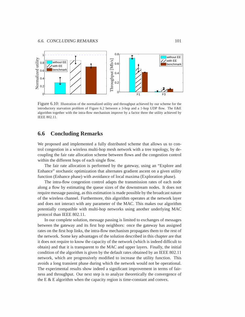
6.6. CONCLUDING REMARKS 101
0
0.2
0.4
0.6
0.8
1
without EEwith EEbenchmark
Nor
mal
ized
utili
ty
F1 F30
0.2
0.4
0.6
0.8
without EEwith EEbenchmark
Thr
ough
put[
Mb/
s]
Figure 6.10:Illustration of the normalized utility and throughput achieved by our schemefor theintroductory starvation problem of Figure 6.2 between a3-hop and a1-hop UDP flow. The E&Ealgorithm together with the intra-flow mechanism improve by a factor three theutility achieved byIEEE 802.11.
6.6 Concluding Remarks
We proposed and implemented a fully distributed scheme that allows us to con-trol congestion in a wireless multi-hop mesh network with a tree topology, by de-coupling the fair rate allocation scheme between flows and the congestion controlwithin the different hops of each single flow.
The fair rate allocation is performed by the gateway, using an “Explore andEnhance” stochastic optimization that alternates gradient ascent on a given utilityfunction (Enhance phase) with avoidance of local maxima (Exploration phase).
The intra-flow congestion control adapts the transmission rates of each nodealong a flow by estimating the queue sizes of the downstream nodes. It doesnotrequire message passing, as this estimation is made possible by the broadcastnatureof the wireless channel. Furthermore, this algorithm operates at the network layerand does not interact with any parameter of the MAC. This makes our algorithmpotentially compatible with multi-hop networks using another underlying MACprotocol than IEEE 802.11.
In our complete solution, message passing is limited to exchanges of messagesbetween the gateway and its first hop neighbors: once the gateway has assignedrates on the first hop links, the intra-flow mechanism propagates them to the rest ofthe network. Some key advantages of the solution described in this chapter are thatit does not require to know the capacity of the network (which is indeed difficult toobtain) and that it is transparent to the MAC and upper layers. Finally, the initialcondition of the algorithm is given by the default rates obtained by an IEEE 802.11network, which are progressively modified to increase the utility function. Thisavoids a long transient phase during which the network would not be operational.The experimental results show indeed a significant improvement in terms of fair-ness and throughput. Our next step is to analyze theoretically the convergence ofthe E & E algorithm when the capacity region is time-constant and convex.
102 CHAPTER 6. JOINT CONGESTION-CONTROL AND FAIRNESS

Chapter 7
Multi-Hop Networks BeyondCapacity
7.1 Background
7.1.1 Problem Statement
The throughput of wireless multi-hop networks has received much attentionin thecase where the network operateswithin the capacity region, but notaboveit. Inthis chapter, we study the answers to this question for IEEE 802.11 networks onthe simplest non-trivial topology, which is a linear network. We chose to focus onthis topology for the following reasons: (i) it is found as a part of almost everywireless multi-hop network; (ii) its capacity region is easy to compute, but thenetwork dynamics may be complex outside the capacity region, as indicated by thenon-monotonic curve of Figure 7.1; (iii) despite the complexity of the dynamics,we can prove the non-monotonicity of the curve of Figure 7.1, first, mathematicallyon a Markov chain model and, next, experimentally through measurements in areal testbed. We compute the different phases that the throughput evolution goesthrough at different input rates, and the values at which the transitions occur.
In order to have a better idea of the counter-intuitive relation between the sourcerateλ and the end-to-end throughputµ, we present simulation results for a4-hopnetwork in Figure 7.1. In this scenario, only node0 (i.e., the source) receivesfresh packets at a rateλ, whereas node1, 2 and3 do not inject any new packetsand solely act as relays for the packets to the destination node4 (see Figure 7.2).We consider that the IEEE 802.11 protocol is used with its standard settings:(i)without RTS/CTS, (ii) with a transmission range of1-hop, and (ii) with a sensingrange of2-hop. In other terms, this means that nodei can successfully transmitonly if the nodesi ± k are silent, withk ∈ {1, 2}. The results show that therelation between the input rateλ and the throughputµ can be divided into threedistinct phases according toλ:
103
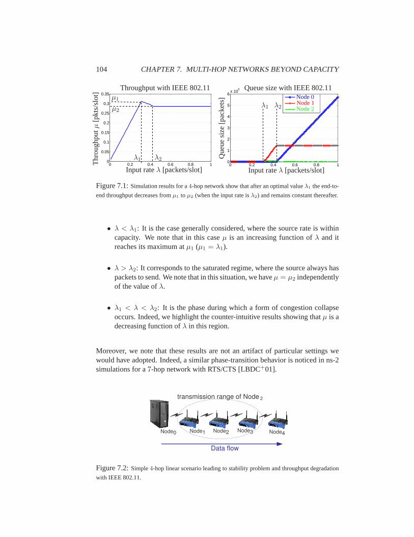
104 CHAPTER 7. MULTI-HOP NETWORKS BEYOND CAPACITY
0 0.2 0.4 0.6 0.8 10
0.05
0.1
0.15
0.2
0.25
0.3
0.35
λ1 λ2
µ1
µ2
Input rateλ [packets/slot]
Thr
ough
putµ
[pkt
s/sl
ot] Throughput with IEEE 802.11
0 0.2 0.4 0.6 0.8 10
1
2
3
4
5
6x 10
5
λ1 λ2
Que
uesi
ze[p
acke
ts] Queue size with IEEE 802.11
Node0Node1Node2
Input rateλ [packets/slot]
Figure 7.1:Simulation results for a4-hop network show that after an optimal valueλ1 the end-to-
end throughput decreases fromµ1 to µ2 (when the input rate isλ2) and remains constant thereafter.
• λ < λ1: It is the case generally considered, where the source rate is withincapacity. We note that in this caseµ is an increasing function ofλ and itreaches its maximum atµ1 (µ1 = λ1).
• λ > λ2: It corresponds to the saturated regime, where the source always haspackets to send. We note that in this situation, we haveµ = µ2 independentlyof the value ofλ.
• λ1 < λ < λ2: It is the phase during which a form of congestion collapseoccurs. Indeed, we highlight the counter-intuitive results showing thatµ is adecreasing function ofλ in this region.
Moreover, we note that these results are not an artifact of particular settings wewould have adopted. Indeed, a similar phase-transition behavior is noticedin ns-2simulations for a7-hop network with RTS/CTS [LBDC+01].
Node1 Node4Node3Node2
transmission range of Node
Data flow
2
Node0
Figure 7.2:Simple4-hop linear scenario leading to stability problem and throughput degradation
with IEEE 802.11.
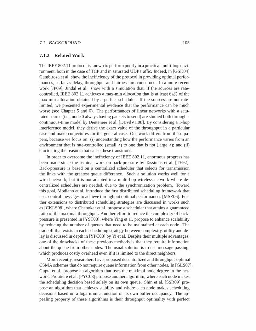
7.1. BACKGROUND 105
7.1.2 Related Work
The IEEE 802.11 protocol is known to perform poorly in a practical multi-hop envi-ronment, both in the case of TCP and in saturated UDP traffic. Indeed, in [GSK04]Gambiroza et al. show the inefficiency of the protocol in providing optimal perfor-mances, as far as delay, throughput and fairness are concerned. In a more recentwork [JP09], Jindal et al. show with a simulation that, if the sources are rate-controlled, IEEE 802.11 achieves a max-min allocation that is at least64% of themax-min allocation obtained by a perfect scheduler. If the sources are not rate-limited, we presented experimental evidence that the performance can be muchworse (see Chapter 5 and 6). The performances of linear networks witha satu-rated source (i.e., node0 always having packets to send) are studied both through acontinuous-time model by Denteneer et al. [DBvdVH08]. By considering a1-hopinterference model, they derive the exact value of the throughput in a particularcase and make conjectures for the general case. Our work differs from these pa-pers, because we focus on: (i) understanding how the performance varies from anenvironment that is rate-controlled (smallλ) to one that is not (largeλ); and (ii)elucidating the reasons that cause these transitions.
In order to overcome the inefficiency of IEEE 802.11, enormous progress hasbeen made since the seminal work on back-pressure by Tassiulas et al. [TE92].Back-pressure is based on a centralized scheduler that selects for transmissionthe links with the greatest queue difference. Such a solution works well for awired network, but it is not adapted to a multi-hop wireless network where de-centralized schedulers are needed, due to the synchronization problem.Towardthis goal, Modiano et al. introduce the first distributed scheduling framework thatuses control messages to achieve throughput optimal performances [MSZ06]. Fur-ther extensions to distributed scheduling strategies are discussed in workssuchas [CKLS08], where Chapokar et al. propose a scheduler that attainsa guaranteedratio of the maximal throughput. Another effort to reduce the complexity of back-pressure is presented in [YST08], where Ying et al. propose to enhance scalabilityby reducing the number of queues that need to be maintained at each node.Thetradeoff that exists in each scheduling strategy between complexity, utility andde-lay is discussed in depth in [YPC08] by Yi et al. Despite their multiple advantages,one of the drawbacks of these previous methods is that they require informationabout the queue from other nodes. The usual solution is to use message passing,which produces costly overhead even if it is limited to the direct neighbors.
More recently, researchers have proposed decentralized and throughput-optimalCSMA schemes that do not require queue information from other nodes. In [GLS07],Gupta et al. propose an algorithm that uses the maximal node degree in the net-work. Proutiere et al. [PYC08] propose another algorithm, where each node makesthe scheduling decision based solely on its own queue. Shin et al. [SSR09]pro-pose an algorithm that achieves stability and where each node makes schedulingdecisions based on a logarithmic function of its own buffer occupancy. The ap-pealing property of these algorithms is their throughput optimality with perfect
106 CHAPTER 7. MULTI-HOP NETWORKS BEYOND CAPACITY
CSMA, but they require very large queue sizes (i.e., in the order of thousands ofpackets), which can seriously degrade delay performances. A different approachis taken by Jiang et al. who introduce an adaptive CSMA algorithm that adjuststhe transmission aggressiveness based on a differential between the arrival and ser-vice rate [JWa]. To summarize, significant theoretical progress has been recentlymade on algorithms that are based on variations of the back-pressure algorithm(i.e., MaxWeight). Nevertheless, we emphasize that MaxWeight is based ontwoassumptions: (i) the set of nodes and the traffic demands are fixed; and (ii) allthe sources are rate limited to transmit only at a rate within the capacity region.In [vdVBS09], van de Ven et al. show that MaxWeight policies might fail topro-vide stability in the case that the first condition is violated, due to the variabilityin the system. Our work differs, because we focus rather on the secondconditionand we are interested in analyzing how the source rate affects the stability ofaIEEE 802.11 multi-hop network. Indeed, the capacity is generally time varyingand difficult to measure exactly in practice [SSGG09]. Hence, it is importanttoknow what type of performance losses can be expected when the sources receivespackets at a rate above the physical capacity of the network (which differs from thelink capacity).
7.1.3 Network Model
We introduce a model that is based on the common assumption of a slotted discretetime axis [CKLS08, ES05, LE99, TE92, YST08, AST09], that is, each transmis-sion takes one time slot and all the transmissions, occurring during a given slot,start and finish at the same time. Moreover, we consider that node0 is the onlysource and that the packets arrive at the source following a random distributionof meanλ. Moreover, the number of arriving packetsξ0(n) is i.i.d (independentand identically distributed) in different time slotsn ∈ N. The destination of allpackets is NodeN , and nodes1 to N − 1 act as relays (ξi>0(n) = 0 for all n).Every node has an infinite buffer for storing messages, and uses FIFOschedulingpolicy, with transmissions from nodei to its nearest right neighbor, nodei + 1.A packet leaves the system once it reaches the destination nodeN . We capturethe restriction linked to the wireless medium by assuming a2-hop sensing range(which eliminates collisions). A nodei can therefore only transmit in a slot if thenodesi± k are not scheduled for allk ∈ {1, 2}.
Under these assumptions, we describe the state of the system by the variables{bi(n), n ∈ N}, with 0 ≤ i ≤ N − 1, wherebi(n) represents the number ofpackets at time instantn in the queue of nodei. At the beginning of each slot thetransmission pattern
~z(n) = [z0(n) z1(n) z2(n) . . . zN−1(n)]
is selected, wherezi(n) = 1 if node i is scheduled for transmission at slotn andzi(n) = 0 otherwise. In order to pick~z(n), each nodei with a non-empty queuecompetes for the access to the channel and picks a uniform backoffβi(n) ∈ [0; 1],
7.2. SIMULATIONS 107
and the nodes with an empty queue setβi(n) = ∞. Next, if there is at least onenode with a non-empty queue, the nodei with the smallest backoff
βi(n) = min0≤j<N
βj(n)
is scheduled for transmission (zi(n) = 1) and the nodes within its2-hop sensingrange are removed from the competition (βi+k(n) = ∞ for k ∈ {0, 1, 2}). Then,the node with the next smallest backoff is selected. This process repeats itself untilno more nodes compete for the channel (i.e.βi(n) = ∞ for all i) and the finaltransmission pattern~z(n) is obtained. We stress that this model is simpler than thereal IEEE 802.11 protocol as we do not take into account the exponential increaseof the contention windowcwi (i.e., the doubling of the contention window afteran unsuccessful transmission). Nevertheless, we note that if IEEE 802.11 is usedwith a fixed contention window (i.e.,CWmin = CWmax = cwi) the protocolselects its backoff uniformly in[0; cwi − 1], which is equivalent to the selectionof βi(n) ∈ [0; 1] in our model. We will validate that the results predicted by thismodel with experiments with the real IEEE 802.11 protocol in Section 7.4. Finally,the dynamics of our system is captured by the relation
bi(n+ 1) = bi(n) + zi−1(n)− zi(n) + ξi(n).
We note that the relationbi(n) − zi(n) is always non-negative, because only thenodes with a non-empty queue (i.e.,bi(n) > 0) can be scheduled for transmission(i.e., havezi(n) = 1).
7.2 Simulations
Before providing a quantitative analysis in the next section, we will first gain aqualitative understanding of the phase transition in throughput atλ1 andλ2 inFigure 7.1, by using time-slotted simulations of the model of Section 7.1.3. For allour scenarios, simulations are repeated to sweep allλ ∈ [0, 1] with increments of0.01. We stress that we assume, without loss of generality, that all the links have acapacity of1 and thus we do not consider the casesλ > 1. The theoretical capacityof the networkλ = 1/3 is reached by a perfect centralized scheduler.
7.2.1 4-Hop Networks
Simulating the4-hop topology of Figure 7.2 for106 slots, we find that the twotransition pointsλ1 = 0.32 andλ2 = 0.43 correspond to two specific behavioralchanges in the queue evolution of the nodes.
Indeed, a perfect centralized scheduler reaches the capacityλ = 1/3 by alwaysscheduling nodes0 and3 concurrently. With IEEE 802.11, there is a non-zeroprobability of having these two nodes scheduled independently (e.g. if exactly oneof these two nodes has an empty queue), which yields thatλ1 < 1/3. We see that

108 CHAPTER 7. MULTI-HOP NETWORKS BEYOND CAPACITY
the transition pointλ1 is the source rate where the queue of node1 starts to build upin the network. Interestingly, it is at the first relay node1 and not at the source node0 where this happens. Because the congestion takes place after the first hop, anyincrease in the source rate beyondλ1 (up toλ2) maps to a proportional decreasein the end-to-end throughputµ. Indeed, as the queue of node0 does not build upfor λ ∈ [λ1, λ2], we have that an increase inλ maps to a proportional increasein the number of packets transmitted by node0. Moreover, the shared nature ofthe wireless medium implies that each time node0 transmits a packet that will bequeued up at node1 (i.e.,λ− λ1 packets per time slot in average), it prevents bothnode1 and node2 to forward the packets waiting in their own queues. Resourcesare thus wasted on the queue build-up of node1 and the end-to-end throughputdecreases linearly withλ.
The pointλ2 corresponds to the threshold rate above which the queue of node0 eventually begins to build up. After this threshold, the input rateλ has no result-ing effect on either the throughputµ or the queue growth at node1, because the(saturated) source always has packets to send anyway and thus an increase onλdoes not make any difference in the network, except that the queue of the sourcegrows faster.
7.2.2 5-Hop Networks
Having shown the relation between the phase transition in the end-to-end through-putµ and buffer build-ups in a4-hop network, we confirm that the relation remainsfor largerK-hop topologies.
Toward this goal, we begin by simulating a5-hop network in the same setting.Our results, depicted in Figure 7.3, show that there are in this case, not two, butthree transition points atλ1, λ2 andλ3. Again, each one of these pointsλi cor-responds to a threshold rate above which a new queue begins to build up in thenetwork.
We note that, in a5-hop network, the first transition pointλ1 = 0.3 occursagain before the theoretical1/3 capacity of the network and this is due to the queuebuild-up at node2. To explain why node2 is the first to have its queue explode,we highlight that it is the only node that cannot transmit concurrently with another(due to the2-hop sensing range). Hence, it has a smaller channel access probabilitythan the other competing nodes and it is the first one to build-up when the sourcerateλ increases.
The second transition pointλ2 = 0.35 is the source rate where node1 startsto build up. We observe that this build-up has two effects: (i) it reduces theslopeof the throughput decrease relatively to the input rateλ; and (ii) it linearly reducesthe amount of buffer build-up at node2. The explanation for the second effect isthat the build-up at node1 implies additional transmissions from node0, whichproportionally reduce the number of transmissions from node1, and as result re-duce the backlog at node2. This also explains the first effect, because the packetsqueued at node2 consume more resources (2 transmission slots) than the packets
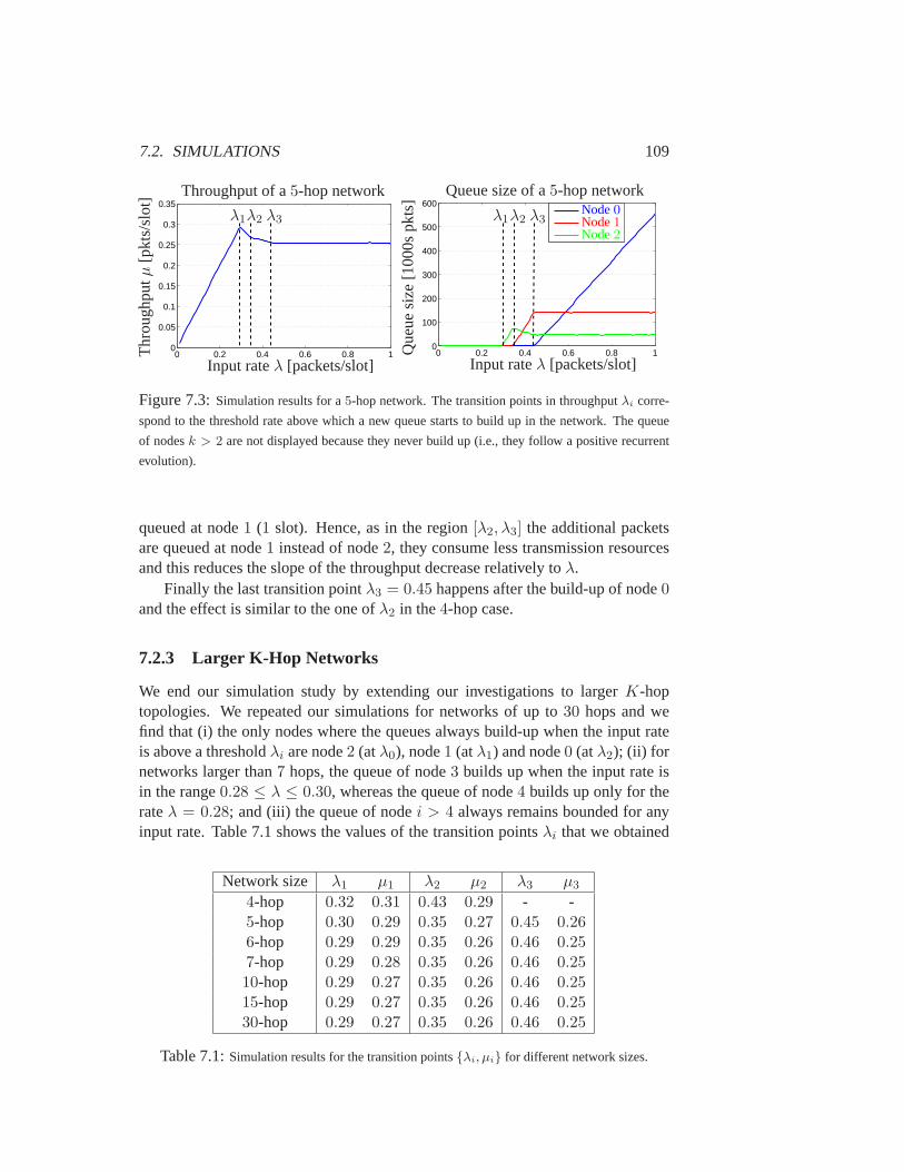
7.2. SIMULATIONS 109
0 0.2 0.4 0.6 0.8 10
0.05
0.1
0.15
0.2
0.25
0.3
0.35
λ1λ2 λ3
Thr
ough
putµ
[pkt
s/sl
ot] Throughput of a5-hop network
Input rateλ [packets/slot]0 0.2 0.4 0.6 0.8 1
0
100
200
300
400
500
600
λ1λ2 λ3
Que
uesi
ze[1
000s
pkts
] Queue size of a5-hop networkNode0Node1Node2
Input rateλ [packets/slot]
Figure 7.3:Simulation results for a5-hop network. The transition points in throughputλi corre-
spond to the threshold rate above which a new queue starts to build up in the network. The queue
of nodesk > 2 are not displayed because they never build up (i.e., they follow a positive recurrent
evolution).
queued at node1 (1 slot). Hence, as in the region[λ2, λ3] the additional packetsare queued at node1 instead of node2, they consume less transmission resourcesand this reduces the slope of the throughput decrease relatively toλ.
Finally the last transition pointλ3 = 0.45 happens after the build-up of node0and the effect is similar to the one ofλ2 in the4-hop case.
7.2.3 Larger K-Hop Networks
We end our simulation study by extending our investigations to largerK-hoptopologies. We repeated our simulations for networks of up to30 hops and wefind that (i) the only nodes where the queues always build-up when the input rateis above a thresholdλi are node2 (atλ0), node1 (atλ1) and node0 (atλ2); (ii) fornetworks larger than7 hops, the queue of node3 builds up when the input rate isin the range0.28 ≤ λ ≤ 0.30, whereas the queue of node4 builds up only for therateλ = 0.28; and (iii) the queue of nodei > 4 always remains bounded for anyinput rate. Table 7.1 shows the values of the transition pointsλi that we obtained
Network size λ1 µ1 λ2 µ2 λ3 µ3
4-hop 0.32 0.31 0.43 0.29 - -5-hop 0.30 0.29 0.35 0.27 0.45 0.266-hop 0.29 0.29 0.35 0.26 0.46 0.257-hop 0.29 0.28 0.35 0.26 0.46 0.2510-hop 0.29 0.27 0.35 0.26 0.46 0.2515-hop 0.29 0.27 0.35 0.26 0.46 0.2530-hop 0.29 0.27 0.35 0.26 0.46 0.25
Table 7.1:Simulation results for the transition points{λi, µi} for different network sizes.
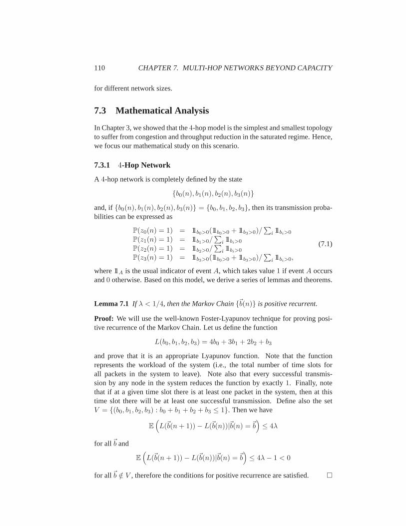
110 CHAPTER 7. MULTI-HOP NETWORKS BEYOND CAPACITY
for different network sizes.
7.3 Mathematical Analysis
In Chapter 3, we showed that the4-hop model is the simplest and smallest topologyto suffer from congestion and throughput reduction in the saturated regime. Hence,we focus our mathematical study on this scenario.
7.3.1 4-Hop Network
A 4-hop network is completely defined by the state
{b0(n), b1(n), b2(n), b3(n)}
and, if{b0(n), b1(n), b2(n), b3(n)} = {b0, b1, b2, b3}, then its transmission proba-bilities can be expressed as
P(z0(n) = 1) = 11b0>0(11b0>0 + 11b3>0)/∑
i 11bi>0
P(z1(n) = 1) = 11b1>0/∑
i 11bi>0
P(z2(n) = 1) = 11b2>0/∑
i 11bi>0
P(z3(n) = 1) = 11b3>0(11b0>0 + 11b3>0)/∑
i 11bi>0,
(7.1)
where11A is the usual indicator of eventA, which takes value1 if eventA occursand0 otherwise. Based on this model, we derive a series of lemmas and theorems.
Lemma 7.1 If λ < 1/4, then the Markov Chain{~b(n)} is positive recurrent.
Proof: We will use the well-known Foster-Lyapunov technique for proving posi-tive recurrence of the Markov Chain. Let us define the function
L(b0, b1, b2, b3) = 4b0 + 3b1 + 2b2 + b3
and prove that it is an appropriate Lyapunov function. Note that the functionrepresents the workload of the system (i.e., the total number of time slots forall packets in the system to leave). Note also that every successful transmis-sion by any node in the system reduces the function by exactly1. Finally, notethat if at a given time slot there is at least one packet in the system, then at thistime slot there will be at least one successful transmission. Define also the setV = {(b0, b1, b2, b3) : b0 + b1 + b2 + b3 ≤ 1}. Then we have
E
(
L(~b(n+ 1))− L(~b(n))|~b(n) = ~b)
≤ 4λ
for all~b and
E
(
L(~b(n+ 1))− L(~b(n))|~b(n) = ~b)
≤ 4λ− 1 < 0
for all~b /∈ V , therefore the conditions for positive recurrence are satisfied.�
7.3. MATHEMATICAL ANALYSIS 111
Lemma 7.2 If λ ≥ 1/3, then the Markov Chain{~b(n)} is not positive recurrent.
Proof: We again use Foster-Lyapunov techniques. Take the function
L(b0, b1, b2, b3) = 3b0 + 2b1 + b2,
which represents the workload of nodes0, 1 and2. Note that the maximal numberof transmissions accomplished by these nodes in one time slot is equal to1, hence,
E
(
L(~b(n+ 1))− L(~b(n)|~b(n) = ~b)
≥ 3λ− 1 ≥ 0
for any vector~b, and the lemma is proved. �
Lemma 7.1 and 7.2 suggest that there exists1/4 ≤ λ1 ≤ 1/3 such that thesystem is stable for allλ < λ1 and unstable for allλ > λ1. We will show thatin fact λ1 < 1/3, which implies that the maximal end-to-end throughput is notachievable by an IEEE 802.11 network.
Theorem 7.1 The value ofλ1 defined above is strictly smaller than1/3.
Proof: We showed already that atλ ≥ 1/3 the Markov chain representing thestate of the system is not positive recurrent, which, in particular, means that thetotal number of packets tends to infinity. However, for our analysis we need moredetailed information, specifically, we need to know at which node the queue build-up occurs.
For this, consider first node0. From the equations about the probability ofnode0 transmitting (i.e.,P(z0(n) = 1)) we conclude that whenever node0 isnon-empty, its transmission probability is larger than or equal to1/3 and whenevernode3 is also non-empty, this probability becomes strictly larger than1/3. Thesetwo facts imply that the number of packets at node0 does not tend to infinity withprobability1, or limn→∞ P(b0(n) = 0) > 0.
Similar arguments allow us to show that atλ = 1/3 the queues of nodes1and2 grow infinitely. Indeed, the total number of packets in these queues growsinfinitely due to Lemma 7.2 and the previously-established fact that the queue ofnode0 stays bounded. Note from (7.1) that the probabilities of transmission ofnodes1 and2 are equal in the case both these queues are non-empty and regardlessof the states of queues0 and3. Indeed, both probabilities are equal to
1
2 + 11b0>0 + 11b3>0,
and hence, the expected change in the queue size of node2 in this case is0. If weassume now thatlimn→∞ P(b1(n) = 0) > 0, then whenever the queue of node1empties, the expected change in the queue size of node2 is negative, which yieldsthat the queue of node2 stays bounded. This contradicts however Lemma 7.2 and

112 CHAPTER 7. MULTI-HOP NETWORKS BEYOND CAPACITY
hence, the queue of node1 grows infinitely. Now we make use again of the factthat whenever both queues1 and2 are non-empty, their transmission probabilitiesare the same, hence, in all these states the expected change in the size of queue2is equal to zero, and hence the queue builds up.
We have now established that atλ = 1/3 the queue of node0 stays bounded,whereas the queues of nodes1 and2 grow infinitely. Assume thatλ1 = 1/3. Thiswould imply that the throughput of the system grows linearly withλ up to the pointλ1 = 1/3 and hence it is equal toµ = 1/3 whenλ = 1/3.
Consider node3 at λ = 1/3. As both nodes1 and2 are non-empty, we havefrom (7.1) that the probability of node3 transmitting in any time slot is equal to
p3 =1 + 11b0>0
3 + 11b0>0,
and the probability of node2 transmitting in any time slot is equal to
p2 =1
3 + 11b0>0.
As λ > 0, the probability for queue of node0 to be non-empty is strictly positive,implying that the queue of node3 stays bounded becausep3 > p2. Note that thisanalysis is valid for anyλ ≥ 1/3, hence the queue of node3 is always bounded.As the queues of nodes1 and2 become infinite atλ = 1/3, the state of the sys-tem may be described by the Markov Chain{b0(n), b3(n)} which has steady-stateprobabilities
p(i, j) = limn→∞
P(b0(n) = i, b3(n) = j).
The throughput of the system (or, equivalently, of node3) can then be written as
µ = 1/3∞∑
j=1
p(0, j) + 1/2∞∑
i=1
∞∑
j=1
p(i, j)
= 1/3P (0, 11) + 1/2P (11, 11) (7.2)
with obvious notationsP (0, 11) andP (11, 11). The throughput of node2 is, how-ever, also equal toµ and to
µ = 1/2P (0, 0) + 1/3P (0, 11) + 1/3P (11, 0) + 1/4P (11, 11)
whereP (0, 0) = p(0, 0) andP (11, 0) =∑∞
i=1 p(i, 0). The two last equationsimply that
P (11, 11) = 4/3P (11, 0) + 2P (0, 0).
The throughput of node0 is equal to1/3 and to
1/3 = 1/3P (11, 0) + 1/2P (11, 11) = P (11, 0) + P (0, 0),
due to the latter equation. Recall now thatP (0, 0)+P (0, 11)+P (11, 0)+P (11, 11) =1 and conclude thatP (0, 11) + P (11, 11) = 2/3. From (7.2) it finally follows that
µ = 1/3P (0, 11) + 1/2P (11, 11) < 1/2(P (0, 11) + P (11, 11)) = 1/3,
and the contradiction proves thatλ1 < 1/3. �
7.3. MATHEMATICAL ANALYSIS 113
Theorem 7.2 If node0 is assumed to be saturated (i.e. to have a packet to transmitat every time instant), then the throughput of the system is equal to2/7.
Proof: We will use an idea from [SdV10]. From the proof of Theorem 7.1 itfollows that nodes1 and2 are also non-empty with probability1, and as the queueof node3 stays bounded, we can introduce time instantsτ0, τ0 + τ1, .., where
τ0 = inf{t > 0 : b3(t) = 0}
and
τi+1 = inf{t > 0 : b3(τi + t) = 0 and there exists 0 < s < t such that
b3(τi + s) > 0}
for i = 0, 1, ... In words, we mark the time instants when node3 becomes empty.Due to the stability of node3, the sequenceτ0, τ1, .. consists of a.s. finite integersthat are independent. Moreover, the random variablesτ1, τ2, .. are identically dis-tributed, and the behavior of the system in each cycle is statistically the same as inany other cycle.
Thus, we can conclude that the throughput of the system is equal to
µ = ET/Eτ1,
whereT is the (random) number of transmissions accomplished by node3 in atypical cycle. Let us now find the expected values ofT andτ . We can write
τ1 = ν0 + ν1,
whereν0 is the time until node2 transmits a packet to node3, andν1 is the timeuntil node3 becomes empty again. First note thatν0 has a Geometric distributionwith parameter1/3. Indeed, when node3 is empty, the other3 nodes compete forthe channel and have equal probabilities (1/3 each) to get the access. Hence, it willtake aGeom(1/3)− 1 time slots until node2 gets the access and then1 more slotfor the transmission itself. Note also that we can write
ν1 =T∑
i=1
ρi,
whereρi is the time taken by node3 to successfully transmit one packet. Note thatthe random variablesρ1, ρ2, .. are independent and each of them has a Geometricdistribution with parameter1/2. Indeed, when all nodes are non-empty, the prob-ability for node3 to successfully transmit in any given time slot is equal to1/2,hence, it will take aGeom(1/2) − 1 time slots until node3 gets access to thechannel and then an additional slot for the transmission. Taking into account ourrepresentations forν0 andν1, we write
Eτ1 = 3 + 2ET. (7.3)

114 CHAPTER 7. MULTI-HOP NETWORKS BEYOND CAPACITY
The expected value of the number of transmissions of node3 over a typical cyclenow remains to be found. For this we will use a method similar to the one used toobtain the value of the expected length of the busy cycle in anM/G/1 queue. Itis clear that every packet that is transmitted by node2 overρ1 − 1 slots generatesits own cycle, and the distribution of the number of successful transmissionsofnode3 in this cycle is exactly the same as the number of successful transmissionsof node3 in the cycleτ1. Moreover, all these cycles are independent. Hence, wecan write
T = 1 +
ρ1−1∑
n=1
11z2(n)=1Tn, (7.4)
where11z2(n)=1 is 1 if node 2 is transmitting at time slotn, and is0 otherwise, andwhere eachTn is distributed asT . Note that in any time slot during the time slotswhen node3 is not transmitting (implying also that node0 is not transmitting),node2 has a probability of1/2 of getting access to the channel (nodes1 and2compete for the channel), which means that
E11z2(n)=1 = 1/2.
This, combined with (7.4), implies that
ET = 1 + 1/2(Eρ1 − 1)ET = 1 + 1/2ET
and, hence,ET = 2.
Plugging this into (7.3) leads to the claim of the theorem. �
Lemma 7.3 There exist aλ2 = 3/7 such that the queue of node0 does not buildup if λ < λ2 and grows infinitely ifλ > λ2.
Proof: We shall concentrate on the caseλ > λ1, so that queues of nodes1 and2are non-empty with probability1. Assume that the queue of node0 is non-empty.We shall use Foster-Lyapunov techniques. Consider
E (b0(τ1)− b0(0)|b0(0) = b0) ,
whereτ1 was defined in the proof of Theorem 7.2. It is clear that duringτ1 timeslots node0 will on average receiveλEτ1 = 7λ new packets. Let us now counthow many packets on average will leave node0 over a typical cycle. Recall therepresentation
τ1 = ν0 + ν1
used in the proof of Theorem 7.2. Note that during theν1 time slots node0 willtransmit exactly as often as node3, i.e., will transmitT (see again the proof ofTheorem 7.2) packets. Among theν0 time slots there areGeom(1/3) − 1 time
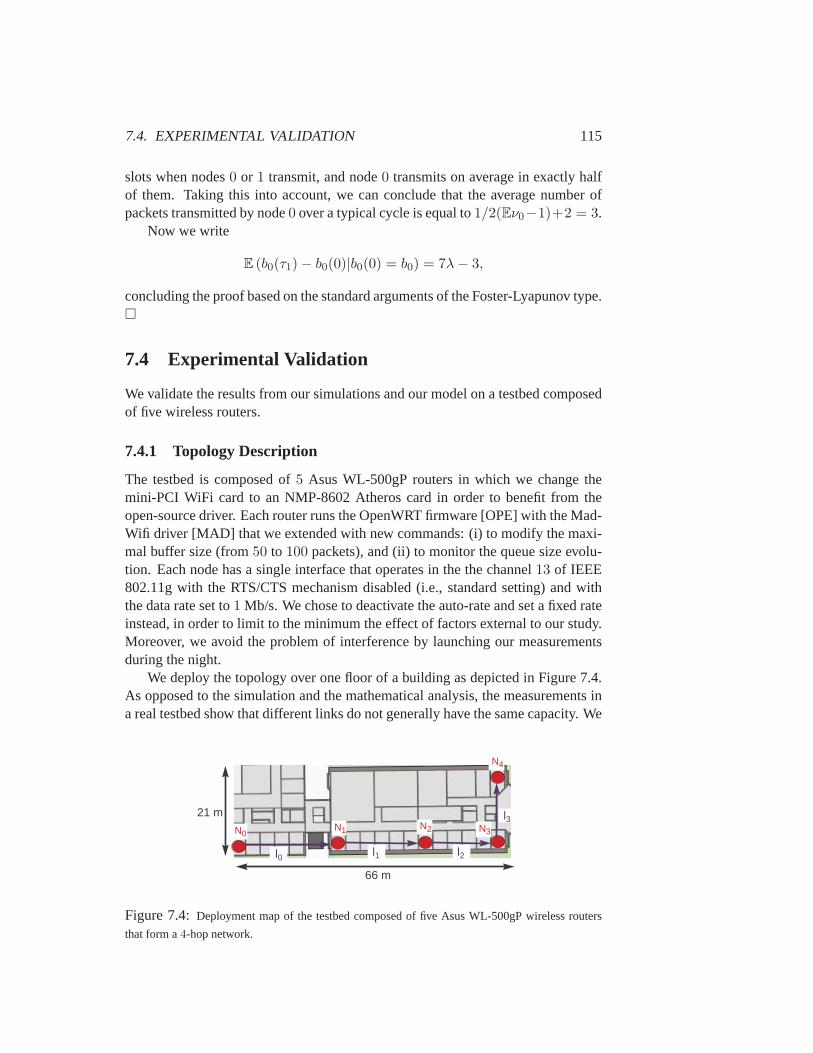
7.4. EXPERIMENTAL VALIDATION 115
slots when nodes0 or 1 transmit, and node0 transmits on average in exactly halfof them. Taking this into account, we can conclude that the average number ofpackets transmitted by node0 over a typical cycle is equal to1/2(Eν0−1)+2 = 3.
Now we write
E (b0(τ1)− b0(0)|b0(0) = b0) = 7λ− 3,
concluding the proof based on the standard arguments of the Foster-Lyapunov type.�
7.4 Experimental Validation
We validate the results from our simulations and our model on a testbed composedof five wireless routers.
7.4.1 Topology Description
The testbed is composed of5 Asus WL-500gP routers in which we change themini-PCI WiFi card to an NMP-8602 Atheros card in order to benefit from theopen-source driver. Each router runs the OpenWRT firmware [OPE]with the Mad-Wifi driver [MAD] that we extended with new commands: (i) to modify the maxi-mal buffer size (from50 to 100 packets), and (ii) to monitor the queue size evolu-tion. Each node has a single interface that operates in the the channel13 of IEEE802.11g with the RTS/CTS mechanism disabled (i.e., standard setting) and withthe data rate set to1 Mb/s. We chose to deactivate the auto-rate and set a fixed rateinstead, in order to limit to the minimum the effect of factors external to our study.Moreover, we avoid the problem of interference by launching our measurementsduring the night.
We deploy the topology over one floor of a building as depicted in Figure 7.4.As opposed to the simulation and the mathematical analysis, the measurements ina real testbed show that different links do not generally have the same capacity. We
N0N1 N2 N3
N4
l0 l1 l2
l321 m
66 m
Figure 7.4:Deployment map of the testbed composed of five Asus WL-500gP wireless routers
that form a4-hop network.

116 CHAPTER 7. MULTI-HOP NETWORKS BEYOND CAPACITY
present in Table 7.2 the link capacity that we measured each minute for660 seconds(i.e., 11 measurement points). From these measurement points, we compute andshow the median value together with the50% confidence interval. We performall our throughput measurements by using theiperf software. From our results,we see that: (i) the linkl2 is the bottleneck of the network and (ii) the2-hopinterference model can accurately capture some practical deployments asit is thecase for the one of Figure 7.4.
7.4.2 Measurement Results
We consider the4-hop flow going from node0 to node4 with the bottleneck inthe3rd hopl2. We perform our measurements by launching traffic at different rateλ for 660 s and measuring the queue evolution and the per-minute throughputµ.Then we compute the median throughput that we depict in Figure 7.5.
First, we note that our experimental results show a similar trend as the simu-lation results introduced in Figure 7.1 (except for the case of the two outliersat1 Mb/s and2 Mb/s that we discuss later). Even though we never have exactlyλ = µ in practice due to the packet losses due to collisions or poor channel condi-tions, we note that the throughputµ increases as a function of the source rate untila first transition pointλ1 = 125 Kb/s (µ1 = 113 Kb/s). Moreover, the logs showthat this transition pointλ1 corresponds to the threshold after which the queue ofone relay node builds up (it is node2 in our experiment due to the low capacity ofl2), before the queue of the source.
This queue build-up is synonym of wasted resources due to the packets thatare lost because of buffer-overflow. It results in a reduction of throughput withµ2 = 102 Kb/s.
Then, we investigate the presence of two outlayers atλ = 1 Mb/s andλ =2 Mb/s. It is interesting to note that, for both rates, the median throughputµ = 108(109) Kb/s is close to the optimum, but with a large confidence interval range.Moreover, our logs show that the queue of the source node0 already builds up(i.e., saturated) at a rate of500 Kb/s. This is even more counter-intuitive as wewould expect that once the source rate is above the saturation threshold of thesource, it would have no influence on the end-to-end throughput. Aftermultiplerepetitions of the experiment to validate this artifact, we conjecture that it is due
Link Median Throughput Confidence Intervall0 836 Kb/s [836− 839]l1 858 Kb/s [857− 863]l2 222 Kb/s [213− 230]l3 830 Kb/s [824− 837]
Table 7.2:Measurements of the link capacityli for each nodei when transmitting alone. We show
the median throughput with the50% confidence interval.
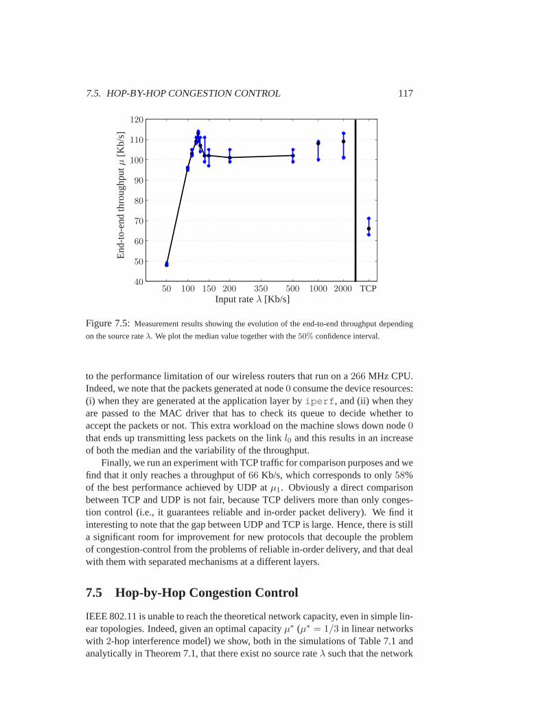
7.5. HOP-BY-HOP CONGESTION CONTROL 117
End
-to-
end
thro
ughp
utµ[K
b/s]
Input rateλ [Kb/s]
50
5040
60
70
80
90
110
120
100
100 150 200 350 500 1000 2000 TCP
Figure 7.5:Measurement results showing the evolution of the end-to-end throughput depending
on the source rateλ. We plot the median value together with the50% confidence interval.
to the performance limitation of our wireless routers that run on a266 MHz CPU.Indeed, we note that the packets generated at node0 consume the device resources:(i) when they are generated at the application layer byiperf , and (ii) when theyare passed to the MAC driver that has to check its queue to decide whethertoaccept the packets or not. This extra workload on the machine slows down node0that ends up transmitting less packets on the linkl0 and this results in an increaseof both the median and the variability of the throughput.
Finally, we run an experiment with TCP traffic for comparison purposes and wefind that it only reaches a throughput of66 Kb/s, which corresponds to only58%of the best performance achieved by UDP atµ1. Obviously a direct comparisonbetween TCP and UDP is not fair, because TCP delivers more than only conges-tion control (i.e., it guarantees reliable and in-order packet delivery).We find itinteresting to note that the gap between UDP and TCP is large. Hence, there isstilla significant room for improvement for new protocols that decouple the problemof congestion-control from the problems of reliable in-order delivery,and that dealwith them with separated mechanisms at a different layers.
7.5 Hop-by-Hop Congestion Control
IEEE 802.11 is unable to reach the theoretical network capacity, even in simple lin-ear topologies. Indeed, given an optimal capacityµ∗ (µ∗ = 1/3 in linear networkswith 2-hop interference model) we show, both in the simulations of Table 7.1 andanalytically in Theorem 7.1, that there exist no source rateλ such that the network
118 CHAPTER 7. MULTI-HOP NETWORKS BEYOND CAPACITY
achieves a throughputµ = µ∗. A key implication of this finding is that it isim-possible for any end-to-end congestion control scheme that runs overIEEE 802.11to be throughput-optimal. This supports the idea that doing congestion control ina hop-by-hop manner, instead of end-to-end, allows the system to reacha higherthroughput. In order to see how well hop-by-hop schemes perform, weanalyzethrough simulations some state-of-the-art scheduling algorithms. We consider thefour following scheduling schemes in addition to IEEE 802.11:
• Policy 1 - IEEE 802.11: Each node with a non-empty queue selects itsbackoff uniformly in the same interval (recall that we do not consider theexponential backoff mechanism)
βi = U(0, 1).
• Policy 2 - linear own queue policy:This policy comes from an algorithmintroduced by Shin et al. for a non-slotted time model [SSR09]. In this algo-rithm a nodei wakes up at a clock tick and if the channel is idle it transmitswith a probability exp(Wi(t))
1+exp(Wi(t)), whereWi(t) is a function oflog(bi+1) with
bi being the queue size of nodei. We simulated a similar policy for a slotted-time system by making each nodei select its backoffβi as a function of itsqueue
βi =1
bi + 1· U(0, 1).
• Policy 3 - logarithmic own queue policy:Another approach studied in [SSR09]is to select the transmission probability depending onWi(t) that is a func-tion of log(log(bi + e)). We captured this policy in a slotted-time systemby making each nodei select its backoffβi as a function of thelog(·) of itsqueue
βi =1
1 + log(bi + 1)· U(0, 1).
• Policy 4 - next-hop queue policy:This policy is inspired from the EZ-flowalgorithm that we presented in Chapter 5. In this scheme each nodei adaptsits transmission probability depending on the queue at the next-hop nodei+1. When the queue at nodei+1 goes above a threshold (i.e.,bi+1 > bmax)the transmission probability is increased (i.e.βi divided by two), and when itgoes below another threshold (i.e.,bi+1 < bmin) the transmission probabilityis decreased (i.e.βi is doubled). In our simulation, we simplify this policyby neglecting the dependence betweenβi(n) andβi(n − 1). Instead, weconsider that each nodei selects its backoffβi as only a function of thequeue at its next hop
βi =
(
1−1
bi+1 + 1 + ǫ
)
· U(0, 1),
for a smallǫ > 0 that is used in order to avoid having exactlyβi = 0 for allthe nodes having their next-hop node with an empty queue (i.e.,bi+1 = 0).
7.5. HOP-BY-HOP CONGESTION CONTROL 119
• Policy 5 - airtime-limiting policy: This policy comes from an algorithmproposed by Jang et al. for TCP traffic in [JPG10]. In their scheme, theauthors find the allocation timeAi of a link li by using the notion of:Ni
(the link li and its interfering links),Wi (the number of flows traversing thelink li), andNWi (the number of flows traversing a link inNi). Finally theallocation is obtained by trading some efficiency for stability (i.e., not takingadvantage of spatial reuse) and computing
Ai =Wi
maxk∈Ni(NWk)
.
Each linkli has then its airtime transmission restricted to be not more than afractionAi of the time.
We study each one of these algorithms and we present the throughput evolu-tion as a function of the input rateλ for multi-hop networks of various sizes inFigure 7.6. We obtain analytically the throughput of the airtime-limiting policyand we simulate the other policies for107 time slots using the same settings as inSection 7.2.
In order to derive the throughput of the airtime-limiting policy (policy5), wenote that we haveWi = 1 for all i and thus we have
−−→NW = [3, 4, 4, 3]
for a4-hop network and−−→NW = [3, 4, 5, 4, 3]
for a5-hop network. That gives a limitation for linkli of Ai = 1/4 for all i in thecase of a4-hop network, andAi = 1/5 for a 5-hop network. The advantage ofthis policy is that it never decreases withλ (i.e., robustness) as opposed to policy1and2. However, this is achieved at the cost of a decrease in efficiency whenUDPtraffic is used. Indeed, when the sources send traffic at exactly the network capacityλ = 1/3 this policy only delivers a throughput of1/4 (75% of the optimum) or1/5(60% of the optimum). One should stress that this scheme was designed for TCP,where robustness to different ratesλ is critical – remember from Section 7.4.2 thatTCP performs poorly over 802.11 linear networks.
As expected, our results show that, in the4-hop case , both policies2 and3 (i.e.,own queue policies) are throughput-optimal when the source rate remains withinthe network capacityλ ≤ 1/3 (i.e., efficiency). For larger topologies, we find inter-esting results as we note that policy2 is still throughput-optimal, whereas policy4appears to suffer a throughput degradation, even though it has beenformally provento be throughput-optimal [SSR09]. This simulation result illustrates the importanceof having very large queues in order for policy4 to be indeed throughput-optimal.Based on these results we can conclude that policy2 is the policy delivering thebestefficiency. However, this is performed at the cost ofrobustnessas we note thatboth policies suffer from throughput degradation when the source receives packets

120 CHAPTER 7. MULTI-HOP NETWORKS BEYOND CAPACITY
at a rateλ > 1/3. Furthermore, we see that this degradation is a serious problemfor the linear case (policy2), but it is less severe with thelog(·) function (policy4). This result supports the proposition of Shin et al. to use thelog(·) as it providesmore robustness that the linear counter-part.
0
0.05
0.1
0.15
0.2
0.25
0.3
0.35
0 0.2 0.4 0.6 0.8 1Thr
ough
putµ
[pkt
s/sl
ot] Throughput of a4-hop network
IEEE 802.11
Policy5Policy2
Input rateλ [packets/slot]
0
0.05
0.1
0.15
0.2
0.25
0.3
0.35
0 0.2 0.4 0.6 0.8 1Thr
ough
putµ
[pkt
s/sl
ot] Throughput of a4-hop network
IEEE 802.11
Policy4Policy3
Input rateλ [packets/slot]
0
0.05
0.1
0.15
0.2
0.25
0.3
0.35
0 0.2 0.4 0.6 0.8 1Thr
ough
putµ
[pkt
s/sl
ot] Throughput of a5-hop network
IEEE 802.11
Policy5Policy2
Input rateλ [packets/slot]
0
0.05
0.1
0.15
0.2
0.25
0.3
0.35
0 0.2 0.4 0.6 0.8 1Thr
ough
putµ
[pkt
s/sl
ot] Throughput of a5-hop network
IEEE 802.11
Policy4Policy3
Input rateλ [packets/slot]
0
0.05
0.1
0.15
0.2
0.25
0.3
0.35
0 0.2 0.4 0.6 0.8 1Thr
ough
putµ
[pkt
s/sl
ot] Throughput of a7-hop network
IEEE 802.11
Policy5Policy2
Input rateλ [packets/slot]
0
0.05
0.1
0.15
0.2
0.25
0.3
0.35
0 0.2 0.4 0.6 0.8 1Thr
ough
putµ
[pkt
s/sl
ot] Throughput of a7-hop network
IEEE 802.11
Policy4Policy3
Input rateλ [packets/slot]
Figure 7.6:Simulations for a multi-hop network with different hop-by-hop schedulingschemes
used for congestion control. Scheduling policies based on a node’s ownqueue (policy2 and3)
reach high throughput at capacity, whereas policies based on either thenext-hop queue (policy4) or
airtime-limiting (policy5) provide robustness to source ratesλ that are above capacity.
7.6. CONCLUDING REMARKS 121
Finally the next-hop queue policy (policy4) results in a nice tradeoff betweenrobustness vs. efficiency. Indeed, it also achieves the robustness property of policy5, and it delivers a throughput that is closer to the optimum and is always betterthan IEEE 802.11 in all the topologies that we tested (we simulated networks up to14 hops).
7.6 Concluding Remarks
The capacity region of a multi-hop network is usually assumed to be known inmost of the recent congestion-control schemes and they, moreover, require thisinformation in order to be throughput-optimal. Nevertheless, contrary to wirednetworks, wireless capacity is time-varying and usually unknown. This makesit almost impossible to know whether a network is operating within the capacityregion or not.
Up to our knowledge, we are the first to study, both analytically and experi-mentally, how a multi-hop network behaves at different source rates eitherbelow orabove the capacity. Our contributions are threefold: (i) we proved the existence ofthe different transition points{λi, µi} (see Figure 7.1) and explained the rationalebehind them; (ii) we formally proved that it is impossible for an end-to-end con-gestion control scheme to be throughput-optimal if it runs over IEEE 802.11; (iii)we studied through simulations some state-of-the-art hop-by-hop congestion con-trol mechanisms and we highlighted the tradeoff betweenoptimality (throughputoptimality) androbustness(no throughput collapse beyond capacity) that should betaken into consideration when designing new hop-by-hop scheduling algorithms.
122 CHAPTER 7. MULTI-HOP NETWORKS BEYOND CAPACITY
Chapter 8
Conclusion
8.1 Discussion of the Results
Throughout this thesis we have focused on the scheduling problem that leads anIEEE 802.11 multi-hop network to be unstable, where we defined instability tohappen when the queue of at least one node in the network builds up indefinitely (inpractice this takes the form of buffer saturation and overflow). First, wevalidatedexperimentally the3-hop stability boundarythat means that in the source-saturatedregime a3-hop network is stable, whereas larger topologies are intrinsically unsta-ble. The effects of this stability boundary have been reported experimentally bysome researchers who stated that ”with current commodity wireless technology itdoes not make sense to handle more than three hops” 1. To the best of our knowl-edge, we are the first to propose an analytical model to understand the root causesbehind these phenomenon. In Chapter 3, we proposed a Markovian modeland weintroduced the notion ofstealing effect. The stealing effect takes the form of col-lisions that are the result of the hidden node situation and non-zero transmissiontime. We showed that, interestingly, these collisions have the beneficial effect ofstabilizing the3-hop network. Indeed, a3-hop network would be unstable if thestealing effect was not accounted for (i.e., if it has a zero probability of occurring).In practice, however, the stealing effect probability is always strictly positive dueto the non-zero transmission times
In addition to explaining the instability problem, we proposed, implementedand evaluated some practical solutions to solve it. The first approach we investi-gated is to perform the congestion control at the MAC layer withEZ-flow. Thekey idea behind EZ-flow is to work in a hop-by-hop manner by using at each nodei two separate modules (i) that passively compute the queue size at the next-hopqi+1, and (ii) that automatically adapt the channel access probability accordinglyby varying the contention window parametercwi. We showed experimentally, an-alytically and through simulations that EZ-flow successfully stabilizes a multi-hop
1Lunar project: http://cn.cs.unibas.ch/projects/lunar/
123
124 CHAPTER 8. CONCLUSION
network without requiring any form of message passing.A second approach that we considered is to perform the congestion control at thenetwork layer instead of the MAC layer. Toward this goal, each nodei uses oneIP queueqji per flowj (a flow is the tuple< src IP ; dst IP > within the mesh).Each IP queue is throttled by a rate limiter of rateρji and all the IP queues are thenscheduled to the MAC queue through a Round-Robin scheduler. Similarly to theMAC approach, the per-flow next-hop queue sizeqji is obtained passively by tak-ing advantage of the broadcast nature from the wireless medium. Nevertheless thechannel access probability is adapted by varying the limiting rateρji instead of theMAC contention windowcwi. This modification allows us to decouple the prob-lem of congestion from contention, because it does not abuse the MAC contentionmechanism when performing congestion control.
In order to complement the hop-by-hop congestion control scheme that oper-ates within a flow, we proposed an additional mechanism that runs at the meshgateway and that achieves a level of fairness between the different flows of themesh. This algorithm calledExplore & Enhance(E&E) optimizes a given util-ity function without having a prior knowledge of the network capacity region. Inorder to perform its task, it runs (i) exploration phases to discover the capacityregion and (ii) enhancement phases to improve the utility by a gradient ascent.E&E does not require network-wide message passing to propagate the ratealloca-tion. Instead, it only uses a broadcast message to inform its direct neighbors of thenew allocation and this information is automatically propagated passively by thecongestion-control scheme. We showed in a real deployment both the practicalityand the efficiency of the E&E algorithm. The exact dynamics during the explorephases, however, are difficult to analyze mathematically and, even in the case ofa fixed capacity region, it is hard to provide a formal proof of convergence to theoptimum. In order to overcome this limitation, we are currently investigating slightvariations of the E&E algorithm that are simpler to study analytically.
After having mostly focused on the source-saturated scenario, we analyzedthe effect of the source rateλ on the end-to-end throughputµ of an IEEE 802.11multi-hop networks. We reported, both through simulations and experimentally,some counter-intuitive results that showed that the relation betweenµ andλ isnon-monotonic. We proposed an analytical model that allows us to derive some re-sults concerning the transition points of the curve showing the relation between λandµ for a4-hop network. Using both our simulations and our mathematical anal-ysis, we showed that if a multi-hop network (4 hops or larger) uses an unmodifiedIEEE 802.11 MAC layer, it cannot reach the network capacityµ∗ for any possiblesource rateλ. This results implies that it is impossible for an end-to-end conges-tion control scheme to be throughput optimal when operating above an unmodifiedMAC layer. It supports, therefore, the idea of performing the congestion controlin a hop-by-hop manner (at the MAC or network layer) rather than end-to-end (at
8.2. POSSIBLE EXTENSIONS 125
the transport layer). As a result, we compare through simulations the performanceof different state-of-the-art methodologies to perform hop-by-hop congestion con-trol in a network. This study showed the important tradeoff that exists betweenefficiency(i.e., throughput-optimality) androbustness(i.e., no throughput collapsewhen the sources attempt to operate at a rate above the network capacity).Cur-rently, most of the work in the literature focus solely on the efficiency part. Thewireless capacity, however, is in practice both difficult to measure exactly and timevarying. Hence, in reality it is almost impossible to guarantee that the sourcesalways operatewithin the capacity region without being too conservative. As aresult, the robustness criteria is at least as important as efficiency and westronglybelieve that it should be evaluated when considering new scheduling schemes forwireless multi-hop networks
Finally, a practical outcome of this thesis is the design and deployment on theEPFL campus of the first large-scale multi-hop testbed based on IEEE 802.11. Ini-tially we planed our network to span over the six buildings of the I&C Department,in order to support our experimental research on wireless mesh network. Further-more, we designed our testbed to be as flexible as possible in order to be abletomeet research needs in other fields. The fact that our testbed was usedin variousother research projects [Epi10, Bec11, JSPF+10, EFLBA10] is an indicator thatwe reached our objective of building an efficient platform to support experimentalresearch. For the future, we plan to continue using the testbed and we arecurrentlylooking at different possible upgrades and extensions.
8.2 Possible Extensions
In this thesis we used our Markovian model to study the stability or instability ofthe network using the Lyapunov-Foster criterion. Furthermore, additional studiesbased on this model provide more detailed information about the network behav-ior. An example of possible extensions has been recently performed by Guilleminet al. [GKvL10]; they further study our model in order to derive various asymptoticexpressions for the stationary large buffer probabilities of a 3-hop network.Another possible direction for the extension of our model is to adapt it to covertopologies more general than the linear ones that we focused on. Indeed, we stud-ied more general topologies through simulations and experiments, but not analyti-cally. The challenge there is that, using our methodology, a network containing Nnodes would be modeled as a random walk inN
N−2 and thus the number of statesto consider in the analysis of the Markov chain would rapidly explode.
The experimental studies we performed on a real wireless multi-hop deploy-ment allowed us to draw attention to the fact that the shared nature of the wirelessmedium brings both new features and new challenges.
126 CHAPTER 8. CONCLUSION
On the one hand, our measurements showed that the multi-hop wireless capacity ishighly variable through time, especially in the indoor setting. This implies that thetraditional static scheduling schemes from wired networks cannot directly be ap-plied to the wireless setting and more adaptive techniques need to be used instead.In this thesis, we followed this methodology both in EZ-flow and the Explore &Enhance algorithm, and we stress that a similar adaptive approach can be adaptedto other protocolsOn the other hand, the shared nature of the wireless medium also implies that ad-ditional information is available at a node (i.e., a node hears more than only thepacket targeted to it). In the original IEEE 802.11 protocol, this information iswasted because at the MAC layer the nodes discard all the packets not targeted tothem. However, the new trend in the network community is to take advantage ofthis free information delivered by broadcast wireless medium. Toward this goal,the nodes are set in the promiscuous mode and use all the sniffed packets inorderto better perform this task. In this thesis, we showed how EZ-flow follows thisstrategy to derive the queue occupancy at the next-hop. Other examplesfollowingthis strategy are found in topics such as in opportunistic routing. Nevertheless,we think that this topic is still in its infancy and there are still many directions toexplore in order to take full advantage of the possibilities offered by the broadcastmedium.
In Chapter 7 we showed that no end-to-end congestion control scheme can bethroughput-optimal if it runs directly above an unmodified IEEE 802.11 layer. Thisresults supports the idea that the congestion control in wireless multi-hop networksshould be performed at the network or MAC layer instead than at the transportlayer. Yet, in practice congestion control is currently performed mostly by TCP atthe transport layer. The key advantages of TCP over UDP are that (i) itperformscongestion control and (ii) it provides reliable in-order packet delivery.Hence, in order to propose a credible alternative to TCP, it should match these twofeatures. In this work, we showed that the first mission of congestion control canbe performed more efficiently in a hop-by-hop manner at the network layer. Thesecond mission of in-order packet delivery is still an open issue and an interest-ing extension of this work would be to develop a transport layer that guaranteesin-order packet delivery without the congestion-control part. Such anew transportprotocol, coupled with a hop-by-hop congestion-control mechanism (such as EZ-flow) would be a serious alternative to TCP in wireless multi-hop networks andwireless mesh networks.
Beside the scheduling problem, the experimental framework that we devel-oped at EPFL is general enough to allow for the extension of our study onwirelessmulti-hop networks into many different directions. Below we describe five differ-ent directions that we studied or that are possible extensions.
Indoor Localization:The problem of localization has been solved outdoors bythe Global Positioning System (GPS), but this technique is not applicable to the
8.2. POSSIBLE EXTENSIONS 127
indoor scenarios. An alternative solution to the indoor localization problem istouse the IEEE 802.11 indoor Access Points (APs) to localize a mobile user [BP00,HLL06, KKCP10]. We consider an approach where the different nodes vary theirtransmission power and we evaluated its efficiency in our testbed2 [Epi10]. Ourresults showed that an important factor for the precision of the estimation is den-sity of the APs. Indeed, the denser the network, the more precise the estimation.We think that this tradeoff would be interesting to investigate analytically in moredetail, in order to derive a mathematical expression of this relation.
Opportunistic Routing:Recently, opportunistic routing algorithms have beenproposed to take advantage of the broadcast nature and the variability ofthe wire-less medium [BM05, RSMQ09, LDFK09]. To evaluate the performance of theseprotocols, most authors only consider throughput. We agree that throughput is im-portant, but we argue that delay and congestion metrics are at least equally impor-tant. Our large-scale multi-hop testbed is an ideal platform to evaluate opportunis-tic as it provides independent routes across different buildings. We are currentlyinvestigating these aspects through a deployment on our testbed [Bec11].Oncethe congestion results are obtained, the next step would be to adapt the techniqueof congestion-control discussed in this thesis to the case of opportunistic routing.The challenge there would be to deal with the fact that the next-hop is not knownbeforehand and that the packets might be forwarded out-of-order.
Security Attacks:In the field of network security a large amount of problemsand solutions have been studied both analytically or through simulations. We thinkthat our testbed would be an adequate platform to evaluate experimentally differentattacks and counter-measures. Indeed, we show in one of our projectsthat it is rel-atively easy to perform ARP spoofing with off-the-shelf hardware3. As of yet, wehave not investigated more complex attacks, but this small example shows that ourexperimental infrastructure can be used as a tool to support experimental researchin this field.
Multi-Channel: In this thesis, we mainly focused on the single-channel sce-nario, but an interesting extension of this work would be to study the similari-ties and differences between single-channel WMNs and the multi-antenna,multi-channel WMNs. Indeed, in the multi-antenna setting there are two approachespossible.In the first approach, a form of graph coloring could be used to set each link toone specific channel so as to maximize the spatial reuse. Following such a strategyimplies that a nodei is very likely to use different channels when communicat-ing with nodei − 1 or i + 1. Therefore, either the queue estimation mechanismof EZ-flow should be adapted accordingly (when the number of channelsis largerthan the number of antennas, this may require an additional interface), or explicitmessages need to be used for a node to inform its previous-hop of its queue size.In the second approach, the number of channels used is the same as the number of
2Aziala testbed - IEEE 802.11 Indoor Localization: http://icawww1.epfl.ch/aziala(Video 3)3Aziala testbed - ARP Spoofing Attack: http://icawww1.epfl.ch/aziala(Video 1 and 2)

128 CHAPTER 8. CONCLUSION
antennas and all the nodes use all their interfaces independently (note that this issimilar to having a single channel of larger capacity). If this methodology is used,the results and solution that we proposed for a single-channel mesh networks arethen directly applicable to this setting.Obviously the first approach could result in higher throughput if the number ofchannels is larger than the number of available interfaces. Unfortunately,the levelof complexity is also higher due to the channel attribution step. It would be there-fore interesting to study both approaches in order to evaluate their performance andto see how the single-channel results apply to this multi-channel setting.
Cooperative APs:As a last extension, we suggest the possibility to considerour entire testbed as an infrastructure WLAN and to study how cooperationbe-tween the APs could help significantly improve the performance [WKSK07].In current deployments, such as the one from the EPFL IT, a user is ableto hearmany access points in his range. Nevertheless, he usually transmits his packets toa single destination AP. In case a packet is not correctly received by thedestinationAP (e.g., due to poor channel conditions), it is retransmitted by the user regardlessif another AP was able to correctly receive the packet or not. Instead, anew alterna-tive could be to have the different APs collaborate (as they are typically connectedto a wired infrastructure), then they would send an acknowledgment if at least oneAP receives the packet correctly.Even though such a mechanism is a relatively drastic change to the currentproto-col, it is still an interesting alternative to evaluate. Indeed, there is an interestinggain that can be obtained from spatial diversity (i.e., different APs experience dif-ferent collision and noise levels). Furthermore it is possible to perform theevalua-tion of such a mechanism in our testbed by implementing new elements in Click4
that (i) send broadcast packets instead of unicast, and (ii) perform the new acknowl-edgment mechanism.
4Click Modular Router: http://read.cs.ucla.edu/click/
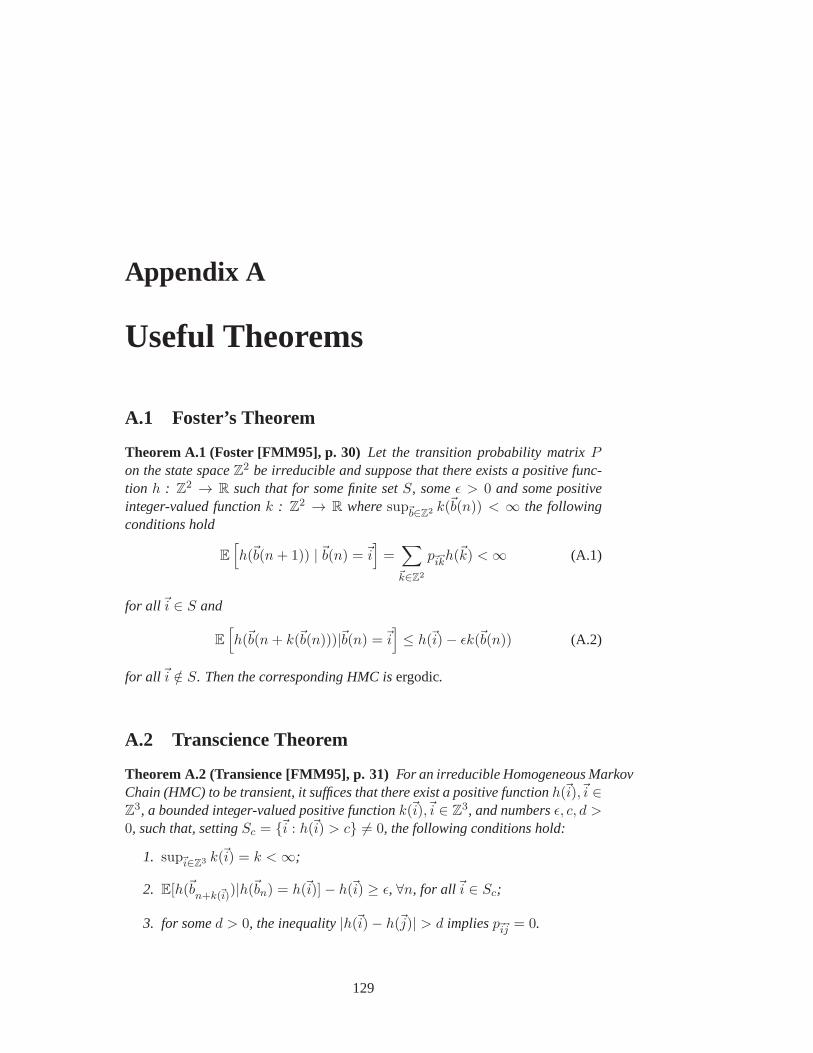
Appendix A
Useful Theorems
A.1 Foster’s Theorem
Theorem A.1 (Foster [FMM95], p. 30) Let the transition probability matrixPon the state spaceZ2 be irreducible and suppose that there exists a positive func-tion h : Z
2 → R such that for some finite setS, someǫ > 0 and some positiveinteger-valued functionk : Z
2 → R wheresup~b∈Z2 k(~b(n)) < ∞ the followingconditions hold
E
[
h(~b(n+ 1)) | ~b(n) =~i]
=∑
~k∈Z2
p~i~kh(~k) <∞ (A.1)
for all ~i ∈ S and
E
[
h(~b(n+ k(~b(n)))|~b(n) =~i]
≤ h(~i)− ǫk(~b(n)) (A.2)
for all ~i /∈ S. Then the corresponding HMC isergodic.
A.2 Transcience Theorem
Theorem A.2 (Transience [FMM95], p. 31) For an irreducible Homogeneous MarkovChain (HMC) to be transient, it suffices that there exist a positive functionh(~i),~i ∈Z3, a bounded integer-valued positive functionk(~i),~i ∈ Z
3, and numbersǫ, c, d >0, such that, settingSc = {~i : h(~i) > c} 6= 0, the following conditions hold:
1. sup~i∈Z3 k(~i) = k <∞;
2. E[h(~bn+k(~i))|h(~bn) = h(~i)]− h(~i) ≥ ǫ, ∀n, for all~i ∈ Sc;
3. for somed > 0, the inequality|h(~i)− h(~j)| > d impliesp~i~j = 0.
129

130 APPENDIX A. USEFUL THEOREMS
A.3 Non-ergodicity Theorem
Theorem A.3 (Non-ergodicity [FMM95], p. 30) For an irreducible HomogeneousMarkov Chain (HMC) to be non-ergodic, it is sufficient that there exist afunctionh(~i),~i ∈ Z
2, a constantd andc, such that the sets{~i | h(~i) > c} and{~i | h(~i) ≤ c}are non-empty, and the following conditions hold for everyn ∈ N:
E
[
h(~b(n+ 1)) | h(~b(n)) = h(~i)]
− h(~i) ≥ 0
for all ~i ∈ {~i : h(~i) > c} and∣
∣
∣E
[
h(~b(n+ 1)) | h(~b(n)) = h(~i)]
− h(~i)∣
∣
∣≤ d
for all ~i ∈ Z2.
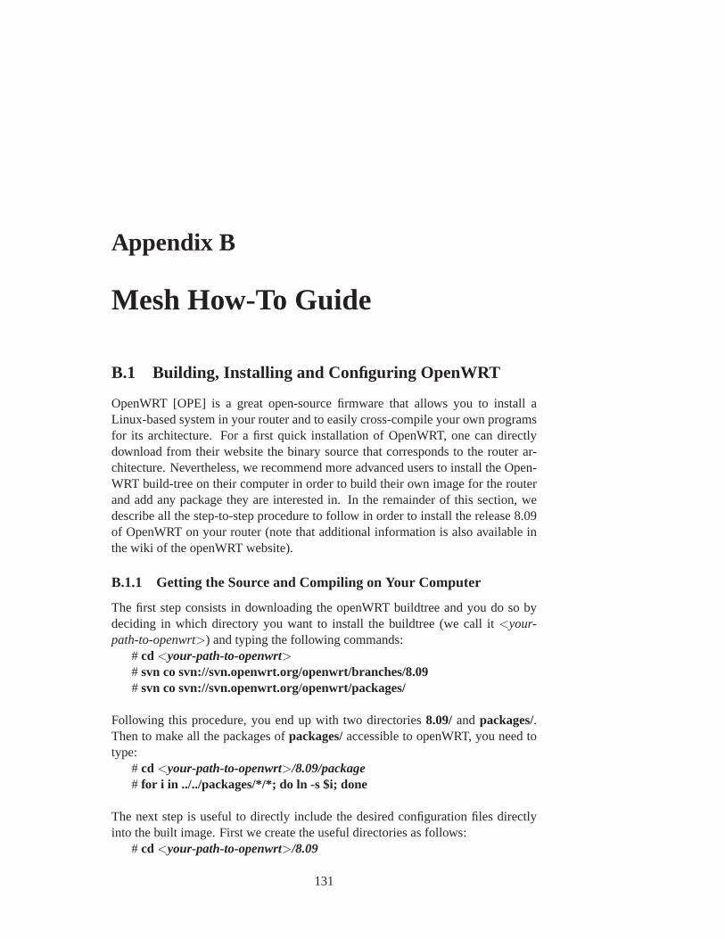
Appendix B
Mesh How-To Guide
B.1 Building, Installing and Configuring OpenWRT
OpenWRT [OPE] is a great open-source firmware that allows you to installaLinux-based system in your router and to easily cross-compile your own programsfor its architecture. For a first quick installation of OpenWRT, one can directlydownload from their website the binary source that corresponds to the router ar-chitecture. Nevertheless, we recommend more advanced users to install theOpen-WRT build-tree on their computer in order to build their own image for the routerand add any package they are interested in. In the remainder of this section, wedescribe all the step-to-step procedure to follow in order to install the release 8.09of OpenWRT on your router (note that additional information is also availableinthe wiki of the openWRT website).
B.1.1 Getting the Source and Compiling on Your Computer
The first step consists in downloading the openWRT buildtree and you do sobydeciding in which directory you want to install the buildtree (we call it<your-path-to-openwrt>) and typing the following commands:
# cd<your-path-to-openwrt># svn co svn://svn.openwrt.org/openwrt/branches/8.09# svn co svn://svn.openwrt.org/openwrt/packages/
Following this procedure, you end up with two directories8.09/ andpackages/.Then to make all the packages ofpackages/accessible to openWRT, you need totype:
# cd<your-path-to-openwrt>/8.09/package# for i in ../../packages/*/*; do ln -s $i; done
The next step is useful to directly include the desired configuration files directlyinto the built image. First we create the useful directories as follows:
# cd<your-path-to-openwrt>/8.09
131

132 APPENDIX B. MESH HOW-TO GUIDE
# mkdir files# cd files# mkdir etc# cd etc# mkdir config# mkdir dropbear# mkdir init.d
Then we create the five following files inside those directories.
1st File: ”files/etc/config/system”
#### Set the hostnameconfig systemoption hostname TAP1
2nd File: ”files/etc/config/network”
#### VLAN configurationconfig switch eth0option vlan0 ”1 2 3 5*”option vlan1 ”0 5”option vlan2 ”4 5”
#### Loopback configurationconfig interface loopbackoption ifname ”lo”option proto staticoption ipaddr 127.0.0.1option netmask 255.0.0.0
#### LAN configurationconfig interface lanoption ifname ”eth0.0”option proto staticoption ipaddr 192.168.1.1option netmask 255.255.255.0
#### DMZ configurationconfig interface dmzoption ifname ”eth0.2”option proto static
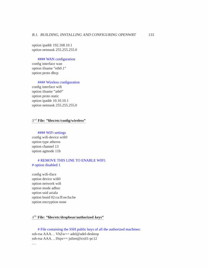
B.1. BUILDING, INSTALLING AND CONFIGURING OPENWRT 133
option ipaddr 192.168.10.1option netmask 255.255.255.0
#### WAN configurationconfig interface wanoption ifname ”eth0.1”option proto dhcp
#### Wireless configurationconfig interface wifioption ifname ”ath0”option proto staticoption ipaddr 10.10.10.1option netmask 255.255.255.0
3rd File: ”files/etc/config/wireless”
#### WiFi settingsconfig wifi-device wifi0option type atherosoption channel 13option agmode 11b
# REMOVE THIS LINE TO ENABLE WIFI:# option disabled 1
config wifi-ifaceoption device wifi0option network wifioption mode adhocoption ssid azialaoption bssid 02:ca:ff:ee:ba:beoption encryption none
4th File: ”files/etc/dropbear/authorized keys”
# File containing the SSH public keys of all the authorized machines:ssh-rsa AAA. . . VhZw== adel@adel-desktopssh-rsa AAA. . . ISqw== julien@icsil1-pc12. . .

134 APPENDIX B. MESH HOW-TO GUIDE
. . .
5th File: ”files/etc/init.d/done”
#!/bin/sh /etc/rc.common# Copyright (C) 2006 OpenWrt.org
# REGULAR TASKS to be done when booting:START=95boot(){[ -d /tmp/root] && {
lock /tmp/.switch2jffsfirstboot switch2jffslock -u /tmp/.switch2jffs
}# process user commands[ -f /etc/rc.local] && {
sh /etc/rc.local}# set leds to normal state. /etc/diag.shset state done
# Then add your OWN TASKS to be done when booting:# TASK 1: Launch WPAifconfig eth0.1 promiscwpa supplicant -c /etc/config/wpasupplicant/wpasupplicant.conf -i eth0.1 -D ro-boswitch -B
# TASK 2: Set the channel rate to 1Miwconfig ath0 rate 1M
#TASK 3: Mount USB drivemkdir /root/mntmount /dev/sda1 /root/mnt}
Once you are done editing the above configuration files, you are almost readyfor cross-compiling in your computer an image that will be ready to be flashedonyour wireless router. The only remaining step consists in selecting your router pro-file (to set for which architecture the compilation should be done) and the programsthat you want to be included as packages in the image. To do so, you need totype:
B.1. BUILDING, INSTALLING AND CONFIGURING OPENWRT 135
# make menuconfigand this makes you enter a pretty intuitive graphical configuration menu with thefollowing categories.
• Target System: This fields allows you to specify the platform of your router.Our Asus WL-500gP routers are based on the Broadcom BCM94704 plat-form, thus we select ”Broadcom BCM947xx/953xx [2.6]”. The number inbracket ([2.4] or [2.6]) is the version of the Linux kernel that is selected. Inthe earlier version of our testbed, we had our routers running the [2.4] ver-sion without any problem. Recently, we flashed all our router with a [2.6]version for a reason of compatibility with the Click package [KMC+00]. Incase you are using other routers than the Asus WL-500gP and do not knowthe platform they are based on, you may find this information on1.
• Target Profile: This field allows you to specify the model of your router.
• Base system: This category allows you to include additional library in theimage of your router (this is useful if you start coding your own programthatrequire a specific library).
• Network: This category provides you with a huge amount of package thatyou can include in your image. However, before adding too many packages,you must keep in mind that the more selected packages, the larger the size ofyour image after compilation and the allowed image size is restricted by theFlash memory of your router (4Mb for most routers and 8Mb for the AsusWL-500gP1). In our testbed, the package we were interested in adding tothe standard configuration are: click, iperf, tcpdump and wpa-supplicant2.
• Kernel modules: This category allows you to include useful modules anddriver. In our case, we were particularly interested in (i) adding the open-source madWiFi driver to our image by selectingkmod-madwifiin the ”Wire-less Driver” directory; (ii) adding USB support to benefit from 2Gb extramemory through USB sticks. To do so, we had to select the moduleskmod-usb-core, kmod-usb-ohci, kmod-usb-storage, kmod-usb-uhciandkmod-usb2in the ”USB Support” directory. Additionally, we also had to include themoduleskmod-fs-ext2, kmod-fs-ext3, kmod-fs-hfs, kmod-fs-vfat, kmod-nls-cp437, kmod-nls-cp850, kmod-nls-iso8859-1in the ”Filesystems” directory.
The above list describes the package that we found, given our needs, the moreuseful to be included in our image. However, it is clearly not an exhaustive descrip-tion of the multiple possibilities of available configurations, and we would recom-mend the interested readers to go quickly through the different categoriesof the
1http://wiki.openwrt.org/oldwiki/tableofhardware2As explained further in Section B.2.3, we are interested to have 802.1X (WPA) available on the
routers. However, the default version available in openWRT does not work with our configuration.Section B.2.3 explains what to do in a scenario similar to ours.
136 APPENDIX B. MESH HOW-TO GUIDE
configuration menu in order to have a clearer idea of what is available. Moreover,if you know the name of a program you would like to include without knowing itslocation on the configuration menu, a useful command is the search command thatis obtained by typing ”/” in the menu.
Now that you are done with the configuration, you are ready to launch your firstcompilation of OpenWRT by typing:
# make V=99where the ”V=99” parameters provides you with all the debugging messages (justtypemake if you do not want to see them). During this first compilation, your com-puter needs to be connected to the Internet as openWRT will download the neededsource code and cross-compile it. All this process takes a pretty long amount oftime for the first compilation, so you may want to launch it over night. Note thatOpenWRT only compiles everything at the first compilation (or if you execute amake clean). In the future compilations, only the modified files will be compiledand thus, the whole process will be significantly faster.
If you followed all the previous steps correctly and went through the compilationprocess without any errors, you should now obtain, in thebin/ directory, differ-ent imagesopenwrt-*.trxandopenwrt-*.bin(the .trx is the one used for the Asusrouter). The next step is then to flash your router with the obtained image andwedescribe two ways of going it either through: (i) TFTP or (ii) SSH.
Flashing the image through TFTP
In order to follow this procedure, you need to start your router in the TFTP mode.For the Asus WL-500gP, this is done by keeping pushed down the RESTORE but-ton (in the back of the router), while plugging in the power cord. If the Asussuc-cessfully started in TFTP mode, you notice it by seeing the READY light blinking.Once in this mode, the router has a TFTP server running that accepts a.trx image(i.e., the firmware) to be flashed. To do so, you need to plug your computer on theLAN port of the Asus router and type the following command
# cd<your-path-to-openwrt>/8.09/bin# tftp 192.168.1.1# tftp> binary# tftp> rexmt 1# tftp> put openwrt-brcm47xx-squashfs.trx
Once the TFTP upload is completed, the router initializes itself with the newfirmware and this is a critical phase. Indeed,do NOT turn off your router dur-ing the2 minutes following the TFTP transfer or you might break it without beingable to recover. After, this2-minute delay, you can unplug the power cord and plugit again and then you can start connecting to your router and configuringit. Fordetails on how to do this, see the Section B.1.1

B.2. EXTENDING OPENWRT WITH SOME USEFUL PACKAGES 137
Flashing the image through SSH
This alternative way of flashing the router can be relatively useful if it happens thatyou can access the router in the normal mode, but not in the TFTP mode (we donot know the cause of this problem, but it sometimes happened to us). To performyour flashing through SSH, you need to plug your computer on the LAN port ofthe Asus router and type the following command
# cd<your-path-to-openwrt>/8.09/bin# scp openwrt-brcm47xx-squashfs.trx [email protected]:/tmp3
# ssh [email protected] once logged in the router TAP1, you type
root@TAP1#mtd write openwrt-brcm-2.4-squashfs.trx linux && rebootAt the end of this process the router will automatically reboot by itself (you donotneed to touch the power plug) and you will be able to connect to it and configure itby following the instruction of next section.
First connection to the router and its configuration
A router that has been just flashed cannot be directly accessed viassh, becausethe connection is blocked. To activate this connection and allow the connectionthrough the wireless and WAN port, you need to set a password and followthefollowing steps:
# telnet 192.168.1.1root@TAP1#passwdroot@TAP1#/etc/init.d/firewall disableroot@TAP1#iptables -F
After this you should be able to connect to your router insshand use your routernormally. Moreover, if for security reasons you want to disable the connection viapassword, you can easily do that by editing the file/etc/config/dropbear.
B.2 Extending OpenWRT with Some Useful Packages
In the previous section, we explained how to build your own image of openWRTby including some of the existing packages directly into the image through themenuconfigwindow. However, one might be interested in adding later on someextra packages to a working router without wanting to go through the process offlashing it once again. In this section, we will show how this can easily be doneand how you can easily cross-compile add your own packages/programsinto themenuconfigwindow.
3Instead of /tmp, you might want to adapt the directory in which you copy theimage in the router.Indeed, you need to copy it onto a volume with enough free space.
138 APPENDIX B. MESH HOW-TO GUIDE
B.2.1 Basics for Adding a Package on your Router
After having compiled openWRT, one can see that many packages (the*.ipk files)are created in the folderbin/packages. Moreover, in case you want to create a new*.ipk file (for example you want to add the vpnc package to an already flashedrouter), you just need to select this package in themenuconfigwindow and to runmake once again. Once the compilation process ends, you have a new packagecreated and you install it following the procedure below (note that this example isfor the Asus router that is built on a mipsel architecture, router based on anotherarchitecture should follow a similar methodology):
# cd<your-path-to-openwrt>/8.09/bin/packages/mipsel# scp vpnc0.5.3-1mipsel.ipk [email protected]:/root# ssh [email protected]
Then once logged in the router TAP1, you simply typeroot@TAP1#opkg install vpnc 0.5.3-1mipsel.ipk
B.2.2 Adding the Click Modular Router
Before describing the procedure of how to cross-compileclick [KMC+00] foropenWRT, we note that this is a relatively big package. Therefore, it mightbe wiseto directly incorporate it in the flashed image instead of installing it afterwards withtheopkg command.
In our deployment, we chose to use the MultiFlowDispatcher library [SL09],which allows to dynamically span sub-element at run time (e.g., in per-flow queu-ing, we only create a queue once a new flow appears in the network). In order tocompile Click with new library included (in this case MultiFlowDispatcher), weneeded (i) to add the filemultiflowdispatcher.cc in<your-path-to-openwrt>/8.09/build dir/mipsel/click-1/lib,(ii) to add the filemultiflowdispatcher.hh in<your-path-to-openwrt>/8.09/build dir/mipsel/click-1/include/click, and(iii) to modify the Makefile in:<your-path-to-openwrt>/8.09/build dir/mipsel/click-1/userlevel/Makefile.inin order to addmultiflowdispatcher.o in theGENERIC OBJS variable.
Now that you know how to cross-compileclick for your router, you might beinterested in adding your own elements to Click. To do so, you might want to reada bit on the basics of how to add an element for click on a computer (i.e., with-out cross-compilation) on the FAQ section of the Click website4. Then once youunderstand this process, the only difference to add your element in the openWRTbuildtree, is that you should add your elements in the folder:
<your-path-to-openwrt>/8.09/build dir/mipsel/click-1/elements/local/
4http://read.cs.ucla.edu/click/learning

B.2. EXTENDING OPENWRT WITH SOME USEFUL PACKAGES 139
Note that during the debugging process of your elements you might need to re-install many times theclick*.ipk package on your router, as any modification ofone of your elements is equivalent to a new version of click that contains thenewelement and that needs to be installed. Personally, we find this procedure rathercumbersome and we even encounter problem re-installing click through the stan-dardopkg command. Instead, we found that a quicker way to re-install click onyour router (that always worked for us) is to simply copy the binary file onyourrouter. This simple technique is performed by typing:
# scp<your-path-to-openwrt>/8.09/build dir/mipsel/click-1/userlevel/[email protected]:/usr/bin/
B.2.3 Adding 802.1x Support for a Secure Wired Connection
Indeed, one of the main goal of wireless multi-hop networks is to avoid usingwires. However, if the network is deployed for research purposes, one shouldconsider connecting the nodes to a wired network in order to be able to controlthem, deploy programs and perform maintenance tasks. If the nodes are deployedwithin your research institution’s building(s), you hopefully will be able to use analready existing wired infrastructure.
In Section 4.3.2 we present an useful way of remotely controlling the nodes.We describe here the procedure that we followed to connect the nodes using thewired network that was already present in the buildings.
Connecting the wireless nodes to a regular wired LAN should not represent abig issue, provided that ethernet interfaces are present on your hardware. However,some institutions require the users of the infrastructure to use secure protocols suchas VPN5 or 802.1X6 (also known as WPA).
We had successful experiences connecting our nodes through VPN with open-WRT, using thevpnc [vpn] open-source VPN client. However, the VPN gatewayis disconnecting the nodes once every couple of hours, changing their IP addresses.A much more convenient way of connecting the routers while using a legacy se-cure protocol available in our institution is to connect the nodes using 802.1X. Thisway, each node is part of the school secure network and has a public IP address thatalmost never changes.
Indeed, such a configuration requires that each node connected to thewirednetwork can access an 802.1X plug. In our case, we had to ask the IT departmentof the university to install one such plug in every office where we were willing toinstall a node, as very few such plugs were active by default.
Once the plugs in place, we installed a WPA (802.1X) client on the nodes. Weuse the well-knownwpa-supplicant program [wpa] for this purpose..
5http://en.wikipedia.org/wiki/Virtual_private_networ k6http://en.wikipedia.org/wiki/IEEE_802.1X
140 APPENDIX B. MESH HOW-TO GUIDE
Here are all the steps that we follow to enable 802.1X authentication withOpenWRT 8.09 :
• Get thewpa-supplicant-0.6.9-2 package provided by Jouke Wit-teveen athttp://www.liacs.nl/ ˜ jwitteve/openwrt/8.09/brcm-2.4/packages/ , or on the Aziala website [AFBT].
• Install it on the nodes using the package manager :opkg install wpa-supplicant 0.6.9-2 mipsel.ipk
• In our case, the config file is/etc/config/wpa supplicant/wpa supplicant.confand it looks like this:
ctrl_interface=/var/run/wpa_supplicantctrl_interface_group=rootap_scan=0network={key_mgmt=IEEE8021Xeap=TTLSidentity="p-aziala"password="xXxXxXxX"phase2="auth=PAP"ca_cert="/etc/config/wpa_supplicant/Thawte_Premium_ Server_CA.pem"priority=5}
Of course, this file is relevant to our own configuration. In particular, the.pem file is the certificate required by the authenticator. In order to avoid tocopy it on every node, we include it in the OpenWRT build tree7.
• The WAN interface is eth0.1 with our configuration. We need to set thisinterface in promiscuous mode :ifconfig eth0.1 promisc
• The command to launch wpa-supplicant is:wpa supplicant -c /etc/config/wpa supplicant/wpa supplicant.conf-i eth0.1 -D roboswitch -B . The option-B is to run wpa-supplicantas a daemon in background.
We added this line at the end of/etc/init.d/done so that the nodesautomatically authenticate on the wired network at boot time.
7files/etc/config/wpa supplicant/Thawte Premium Server CA.pem

B.2. EXTENDING OPENWRT WITH SOME USEFUL PACKAGES 141
B.2.4 Adding your Own Program/Package
Now that you master the technique of including existing program, you might beinterested in including your own program (for exampleHelloWorld.c) in the open-WRT tree in order to cross-compile it and produce a niceHelloWorld.ipkfile thatyou will be able to install on your router and share with other people. To achievethis goal, you have to follow the procedure below:
1. Create the OpenWRT Makefile: The role of the Makefile is to make yourpackage appear correctly in themenuconfigand to tell the cross-compilerwhere it should look for the source code (most likely locally for your owncode, but it can also be online if you provide an URL). The Makefile for yourprogram (here HelloWorld) is easily created by typing:# cd<your-path-to-openwrt>/8.09/package# mkdir HelloWorld# cd HelloWorld# cat> Makefile
include $(TOPDIR)/rules.mk
PKG NAME:=HelloWorldPKG VERSION:=1PKG RELEASE:=1
PKG SOURCE:=$(PKGNAME)-$(PKG VERSION).tar.gz
include $(INCLUDEDIR)/package.mk
define Package/HelloWorldSUBMENU:=CSECTION:=langCATEGORY:=LanguagesTITLE:=Simple ”Hello World” Program# URL:=http://website/.../helloworld# DEPENDS:=+libpcap @!mipsendef
define Package/HelloWorld/descriptionHelloWorld is a basic program that prints the message ”Hello World” onstandard outputs and then exits.endef

142 APPENDIX B. MESH HOW-TO GUIDE
define Build/Compile$(MAKE) -C $(PKG BUILD DIR) \CPPFLAGS=”$(TARGETCFLAGS) -I$(STAGINGDIR)/usr/include -I$(STAGINGDIR)/include”\allendef
define Package/HelloWorld/install$(INSTALL DIR) $(1)/usr/bin$(INSTALL BIN) $(PKG BUILD DIR)/HelloWorld $(1)/usr/bin/$(INSTALL DIR) $(1)/usr/share/HelloWorldendef
$(eval $(call BuildPackage,HelloWorld))
2. Put your source code in the buildtree: To do so, you first need to createthe.tar.gz file that contains your program with its Makefile (note that this isa second Makefile different from previous point). For our Asus based on themipsel architecture, you create thisHelloWorld.tar.gz file by doing:#> mkdir HelloWorld-1#> mv HelloWorld.c HelloWorld-1#> cd HelloWorld-1#> cat> Makefile
CC = mipsel-linux-uclibc-gcc
all:$(CC) HelloWorld.c -o HelloWorld
#> cd ..#> tar czf HelloWorld-1.tar.gz HelloWorld-1/#> mv HelloWorld-1.tar.gz <your-path-to-openwrt>/8.09/dl
Once you follow this process, you should be able to see and select your pack-age through themenuconfigwindow. After selecting it and launching a compi-lation with make, you should see your package HelloWorld.ipk created under thebin/packages/mipseldirectory and you can then install this*.ipk file using the stan-dard procedure shown at the beginning of this section.
B.3. HACKING THE MADWIFI DRIVER 143
B.2.5 Cross-compiling your Program without Making a Package
Creating a package is a cleaner way to transfer your program into OpenWRT. Nev-ertheless, you might be interested in the first debugging phase to quickly compileyour program without going through the work of dealing with the Makefiles.
If that is the case, you can also easily compile your program by using thecross-compiler that are available int thestagingdir directory from your Open-wrt buildtree. For example, in the case you want to compile your program Hel-loWorld.c (or HelloWorld.cpp) for the Asus WL-500gP router (mipsel architec-ture), you only need to type:
#cd<your-path-to-openwrt>/8.09/stagingdir/toolchain-mipselgcc4.1.2/bin/# ./mipsel-linux-uclibc-gcc HelloWorld.c -o HelloWorld# HelloWorld [email protected]:/root/mnt
B.3 Hacking the MadWiFi Driver
B.3.1 Unlocking the Modification of MAC Parameters
The IEEE 802.11e uses four different classes of service: Best Effort (BE), Back-ground (BK), Voice traffic (VO), and Video traffic (VI). Nevertheless, by defaultin IEEE 802.11, all the traffic is queued as BE traffic. Moreover the parametersfor BE traffic are locked by default in the MadWifi driver and this prevent us fromchanging MAC parameters such asCWmin, CWmax, etc. In order to unlock thesemodifications, the MadWifi driver needs to be hacked by commenting the corre-sponding part of the code in the functionieee80211wme updateparams locked()of madwifi-trunk-r3314/net80211/ieee80211proto.c. Note that a patch contain-ing all the needed modification is available at8.
B.3.2 Enabling MadWifi to Announce the FULL BUFFER Status toUpper Layers
By default MadWifi does not inform the upper layer when its queue is full and itdirectly discards the packet instead. This is pretty annoying if one plans to use anadditional queue at the IP layer (for example with Click). Indeed this queuewillalways be empty, because it will always gives any new packet to the MACqueueregardless of whether the MAC queue has space to accept new packetsor not.
In order to overcome this problem, we patch the driver by modifying some filesboth in MadWifi and Linux.First, in MadWifi the files that need to modified are
• madwifi-trunk-r3314/net80211/ieee80211output.c.
• madwifi-trunk-r3314/net80211/ieee80211proto.h.
8http://icawww1.epfl.ch/aziala/P1unlock BEparammodif.patch

144 APPENDIX B. MESH HOW-TO GUIDE
In ieee80211output.c the modifications take place in the methodsieee80211hardstart()andieee80211parent queuexmit() (that has its return value changed from voidto int). These changes consist in returning a value (i.e., an int) in order to telltheupper layer if the MAC has space available in its queue to accept new packets ornot. Finally, the change inieee80211proto.h consists simply in updating the typeof the functionieee80211parent queuexmit() from void to int.Then in Linux, the modifications consist in using this new feedback deliveredby the MAC in order to only transmit a packet to the MAC if it has enoughroom to accept it. The modifications of the code take place in the fileslinux-2.6.26.8/net/core/dev.candlinux-2.6.26.8/net/packet/afpacket.c.For the readability of this report we do not discuss all the changes here,but we pro-vide the links for the patch we created with details modification both for MadWifi9
and for Linux10.
B.3.3 Adding New Commands to Access MAC Parameters
In our research, we were particularly interesting in knowing the queue occupancyof a node, but unfortunately this information is not given by default by theMACdriver. In order to satisfy our needs, we hacked the MAC driver in order to addsome new commands that allow to:
• Enable/disable the use of the4 MAC queues existing in IEEE 802.11e (bydefault this is disable).
• Get/Set the maximal MAC buffer size (by default this is50 packets).
• Access the current MAC queue occupancy.
In order to achieve this goal, we extended thewlanconfigcommand with our owncommands, and we note that a similar methodology than the one we used can beuse to access/modify some other parameters of interest. More specifically, the filesthat we needed to modify to reach our objectives were3 files in the foldermadwifi-trunk-r3314/ath/ (see the details in11)
• if ath.c
• if athioctl.h
• if athvar.h
2 files in the foldermadwifi-trunk-r3314/net80211/(see the details in12)
• ieee80211output.c
9http://icawww1.epfl.ch/aziala/P22 enablefullBuffer MACsignal madwifi.patch10http://icawww1.epfl.ch/aziala/P21 enablefullBuffer MACsignal linux.patch11http://icawww1.epfl.ch/aziala/P31 enableadditionalMACcommands.patch12http://icawww1.epfl.ch/aziala/P32 enableadditionalMACcommands.patch
B.4. INSTALLING AND USING NET-CONTROLLER 145
• ieee80211var.h
and1 file in the foldermadwifi-trunk-r3314/tools/ (see the details in13)
• wlanconfig.c
B.4 Installing and Using Net-Controller
B.4.1 Installation
You can download Net-Controller from Sourceforge14. The latest version of thecode can be downloaded with SVN using the following command:
svn co https://netcontroller.svn.sourceforge.net/svnr oot/netcontrollernetcontroller
Since the user interface is written in Python, it does not require to be compiled.One simply needs the following installed on the machine:
• Python (>= 2.5)
• PyQT
• Matplotlib
Then, once in the source folder of the user interface (/ui ), it suffices to launch:
python NetController.py
cidaemon needs to be compiled in the following way (usinggcc in this ex-ample):
$YOURGCC -Wall -lm -pthread -o cidaemon cidaemon.c
Where$YOURGCCdenotes your version ofgcc .
B.4.2 Configuration
Net-Controller uses one main configuration file and needs at least one map file, thatmaps node indexes to IP addresses.
13http://icawww1.epfl.ch/aziala/P33 enableadditionalMACcommands.patch14http://sourceforge.net/projects/netcontroller/

146 APPENDIX B. MESH HOW-TO GUIDE
netcontroller.cfg
The filenetcontroller.cfg describes the main options of the program. Weexplain them here.
• interval is the period (in seconds) between two updates of the plots.It can be useful to increase the plot update interval when the control net-work has large delays. However, setting intervals smaller than a typical RTTshould not hurt much (although in this case the curves may be drawn in grayif the values are not received fast enough from the network).
• flow interval is the period between two updates of the list of flows.This typically does not need to be small.
• log dir is the directory in which the logs of the commands launched onthe nodes will be saved.
• trace dir is the directory in which the traces containing all the values thathave been plotted.
• map is the name of the file that contains the mapping between the nodeindexes and their IP addresses on the control network. Specifying a validfile name is mandatory here, as pretty much every operations done by Net-Controller requires to communicate with the nodes through the control net-work.
• trafficMap is the name of the file that contains the mapping between thenode indexes and their IP addresses on the actual wireless network. This isused by the traffic manager of Net-Controller in order to start/stop traffic.
• max commands is the maximum number of simultaneous running com-mands. Each command is launched in a separate thread. If the limit isreached, new commands will wait until running commands are done. Avalue around 100 is probably good for most situations.
• default nbPoints is the default number of points of the plots. For ex-ample, if the update period is one second, adefault nbPoints valueof 60 means that the plots will represent the values received during the lastminute, by default. Indeed, this value can be changed by the user once theGUI is launched.
• direct time represents the direction of the time in the plots. If ’True’(direct time), the plot moves from right to left. If ’False’ (reverse time), theplot moves from left to right.
• ip is the IP address of the central host that runs Net-Controller on the controlnetwork.

B.4. INSTALLING AND USING NET-CONTROLLER 147
• port is the UDP port on which the user interface on the central host islistening. This is used to receive the values to plot and the lists of flows.
• client port is the UDP port on which the nodes of the network are lis-tening (on the control network). This is used to transmit the requests for thevalues to plot, or the requests for the lists of flows.
B.4.3 Using the Graphical Interface
In Net-Controller, the nodes are represented by integer indexes. Afterhaving spec-ified a set of indexes, one can choose actions to perform related to thesenodes. Themain actions that are available at the time of writing are related to plots, commandsor traffic.
The nodes one which perform actions can be selected on the left of the GUI(’Nodes’ section). Shortcuts for selecting the nodes with indexes 1 to 4, all thenodes at once, or the node with the highest index, are provided in the form of check-boxes. To select any arbitrary set of nodes, one should use the ’other’ textbox. Inthis textbox, it is possible to specify simple regular expressions. Set of contiguousindexes are noted using “-” between the smallest and the highest index, and severalsuch expressions can be combined separated by “,”. For example, if one wants toselect the nodes{3, 5, 6, 7, 8}, the expression to use is “3,5-8 ”.
Plotting stuff
The section ’Live plots’ allows to select one or several parameters to plot.A pa-rameter is just a keyword that uniquely identifies a quantity to plot. The ’Plot!’button opens a new window representing a plot of all the indicated parameters asmeasured in each of the selected nodes. The GUI offers shortcuts in the formof checkboxes for three parameters. ’CW’ denotes the value of the IEEE 802.11CWmin parameter, read directly from the Madwifi driver. For example, in ourprevious example, if one checks this box and clicks the ’Plot!’ button, a windowwill appear showing the temporal evolution ofCWmin for each one of the nodes{3, 5, 6, 7, 8}. The parameter ’buffer’ denotes the occupancy of the MAC layersending queue (here to, as read from Madwifi).
The parameter ’throughput’ is a bit particular. Indeed, the throughputs thatthe nodes measure are related to the notion of flow. A flow denotes a tuple<IPsource, IPdestination >. All the measured throughputs areper flow, that meansthat the throughput represents what the selected nodes have received for this flow.That also means that the parameter has to denote the flow in which one is interestedin. All the nodes of the network report to Net-Controller the flows they are awareof, and Net-Controller assigns unique IDs to the flows and displays them in the’Flows’ section of the GUI. Now, if one wants to plot the throughput flow withIDi, the name of the parameter is ’thr%F i’. The checkbox ’throughput’ is simply a

148 APPENDIX B. MESH HOW-TO GUIDE
shortcut for ’thr%F0 ’.
It is possible to plot several parameters for the set of selected nodes. However,the parameters have to denote the same thing (i.e., use the same unit, since the samey-axis is used). It is currently only possible to plot several throughputs values (i.e.,for several different flows) on one plot window.
An other particularity of Net-Controller is that it allows to plot parameters thatare read through a Click socket [KMC+00]. In this case, a parameter name ofthe form ’click->element.handler ’ will plot the temporal evolution of thehandlerhandler of the elementelement (see Click documentation for moredetails about elements and handlers [KMC+00]).
If nothing is specified in the ’number of points’ textbox, the default value forthe number of points will be used. If the number of points is 1, the plot will displaybars instead of curves.
By default, all the values that are plotted are locally stored in trace files, in thedirectory specified by thetrace dir option. If nothing is specified in the ’filename’ textbox, a default name (that takes into account the exact creation timeandselected nodes/parameters) will be used.
Sending commands
Once a set of nodes is selected in the ’Nodes’ section, one can send somecom-mands to all of them. By default, the checkbox ’send it over ssh (as root)’ischecked. That means that all the commands that are typed in the textbox will besent with ’ssh root@%IP ’ prepended to them, where ’%IP’ denotes the IP ad-dress of the node to which the command is sent. For this to work properly, yourpublic key should be present in the ’authorized keys ’ file related to the SSHconfiguration present on the nodes (for more details on how to setup SSH,see Sec-tion B.1). If you don’t want to prepend ’ssh root@%IP ’ (for example if theuser that you want to use on the nodes is not root), you can uncheck thebox. In thiscase, you can launch commands over the whole set of selected nodes using the fol-lowing pre-defined variables: ’%IP’ (the IP address of the node) and ’%INDEX’ (itsindex). For example, if you want to create a local directory for each selected node,you can enter something like ’mkdir dir %INDEX. If you want to send a set ofSSH commands with a custom user, sayjoe , you can enter something like ’sshjoe@%IP your-command ’. If you want to systematically be able to send SSHcommands asjoe , you should modify the prefix string in thesendCommand()method of Net-Controller (in the fileNetController.py ).
In addition, Net-Controller allows to send a special kind of commands to inter-
B.4. INSTALLING AND USING NET-CONTROLLER 149
act with Click handlers [KMC+00]. A commands such as ’click<-element.handler=value ’will set the handlerhandler of the elementelement to the valuevalue (seeClick documentation for more details about elements and handlers [KMC+00]).
The status of the command for each of the selected nodes is displayed in the’status’ textbox. The status can be among the three following states:
• running... : the command did not return yet.
• done : the command returned with an exitcode equals to zero.
• failed : the command returned with a non-zero exitcode.
For each command that is launched, itsstdout and stderr outputs areappended to a file that contains such outputs for all the commands launched onthe same node. These files are located in the directory indicated by thelog diroption. If the checkbox ’Auto display output of command’ is checked (which isthe case by default), the part of this file that concerns the last command is read anddisplayed on the right textbox once the command returns. That allows the user toquickly see the outputs of the commands.
The traffic manager
The traffic manager can be send through the menuFile -> Launch trafficmanager or with the keyboard shortcutCtrl+T .
The goal of the traffic manager is to easily start/stop traffic between the nodesof the wireless network. Theiperf program15 is used to generate the traffic.Therefore, it is needed at the nodes for the traffic manager to work. The way thetraffic manager works is rather simple. One simply has to specify a few optionsrelated to the traffic that is about to be generated, click the ’Start’ button. Clicking’Start’ displays a new line after the current one, that allows to generate a new flow.Once a flow is properly running, its ’status’ turns to ’On’ and the button on theright becomes ’Stop’. Clicking ’Stop’ stops the flows. It actually kills each Iperfand SSH processes individually. Therefore, it is highly recommended to wait forthe status on this line to be ’Off’ before trying to start a new flow.
The different option for the flow generation are:
• ’source(s)’: That represents a set of nodes, that can be written using the sameregular expression than for inputing the set of nodes on the main GUI (seeSection B.4.3). Aniperf client process will be launched in each of thesenodes.
• ’destination’: The node that acts as the traffic sink. Aniperf server processwill be launched on this node.
15https://sourceforge.net/projects/iperf/

150 APPENDIX B. MESH HOW-TO GUIDE
• ’port’: The port to use. For the moment, only UDP traffic is implemented.The input for setting TCP instead should be added anytime soon. Enteringnothing here will select ports automatically (from 6000 and incrementing foreach new flow).
• ’duration (s)’: The duration of the traffic in seconds. Nothing defaults to100,000 seconds.
• ’ToS’: The type of service. Can be one of the four values recognizedby theMAC layer (BK, BE, VI, VO). Default is BE (the usual Best Effort trafficclass).
• ’throughput (Mbit/s)’: The desired throughput can be set using a float orinteger value.
Publications
Conference papers
• A. Aziz, S. Shneer, and P. Thiran.Wireless Multi-hop Networks BeyondCapacity. Submitted for publication.
• A. Aziz, J. Herzen, R. Merz, S. Shneer, and P. Thiran.Explore, Enhanceand Propagate: Fair Congestion Control in Wireless Mesh Networks.Submitted for publication.
• A. Aziz, M. Durvy, O. Dousse, and P. Thiran.Models of 802.11 Multi-HopNetworks: Theoretical Insights and Experimental Validation.In Proc. of ACM COMSNETS, Bangalore, India, January 2011.
• A. Aziz, D. Starobinski, P. Thiran, and A. El Fawal.EZ-Flow: RemovingTurbulence in IEEE 802.11 wireless Mesh Networks without MessagePassing.In Proc. of ACM CoNEXT, Rome, Italy, December 2009.
• Adel Aziz, David Starobinski and Patrick Thiran.Elucidating the Instabil-ity of Random Access Wireless Mesh Networks.In Proc. of IEEE SECON, Rome, Italy, June 2009.
• A. Aziz, A. El Fawal, J.-Y. Le Boudec, and P. Thiran.Aziala-net: De-ploying a Scalable Multi-hop Wireless Testbed Platform for ResearchPurposes.In Proc. of Mobihoc S3, New Orleans, LA, USA, May 2009.
• A. Aziz, R. Karrer, and P. Thiran.Effect of 802.11 adaptive ExponentialBackoffs on the Fluidity of Downlink Flows in Mesh Networks.In Proc. of WinMee, Berlin, Germany, March 2008.
• A. Aziz, T. Huehn, R. Karrer, and P. Thiran.Model validation throughexperimental testbed: the fluid flow behavior exampleIn Proc. of Tridentcom, Innsbruck, Austria, March 2008.
• M. Raya, A. Aziz, and J.-P. Hubaux.Efficient secure aggregation in VANETs.In Proc. of VANET, Los Angeles, CA, USA, September 2006.
151
152 PUBLICATIONS
Journal paper
• Adel Aziz, David Starobinski and Patrick Thiran.Understanding and Tack-ling the Root Causes of Instability in Wireless Mesh Networks.Accepted for publication in IEEE/ACM Transactions on Networking.
Demos, Posters and Reports
• A. Aziz, and J. Herzen.A Practical Hand-on Guide for Deploying aLarge-scale Wireless Multi-hop Network.Technical Report, EPFL-REPORT-160176, November 2010.
• J. Herzen, A. Aziz, and P. Thiran.Demo Abstract of Net-Controller: aNetwork Visualization and Management Tool.In Proc. of Infocom, San Diego, CA, USA, March 2010.
• A. Aziz, R. Karrer, and P. Thiran.Promiting Fluidity in the Flow of Pack-ets of 802.11 Wireless Mesh Networks.In Proc. of CoNEXT, New York, NY, USA, December 2007.
Patent
• Aleksandar Damnjanovic, Adel Aziz, and Tao Luo.Semi-persistent schedul-ing for traffic spurts in Wireless Communication. WO/2008/024890QUALCOMM Incorporated, 2008.

Curriculum Vitæ
Adel Aziz was born in 1983 in Lausanne, Switzerland. In October 2006,he earnedhis M.Sc. degree in Communication Systems from Ecole Polytechnique Federalede Lausanne (EPFL) with a specialization in Network and Mobility, and a minorin Management of Technology. With an interest in managerial topics in additiontoscientific research, he used the online course materials to pass the exams and earnhis M.Sc. in Management from HEC Lausanne, in 2009. During his undergraduatestudies, in 2003/2004, he was selected for EPFL’s exchange program;he spent oneyear at Carnegie Mellon University (CMU) in Pittsburgh, Pennsylvania.
In 2006, he successfully completed his master’s thesis at the Corporate R&Ddepartment of Qualcomm Inc. in San Diego, California. During his six months atQualcomm, he worked on scheduling algorithms for VoIP traffic in LTE.
In November 2006, he joined the Laboratory for Computer communicationand Applications (LCA), where he worked on his thesis under the supervision ofProfessor Patrick Thiran. There, he collaborated closely with DeutscheTelekomLaboratories (T-Labs), who funded his research.
During his Ph.D. work, he was a teaching assistant for the classes of StochasticModels for Communication and Oriented Programming. In addition, he supervisedeight students for their master’s theses and semester projects.
In 2010, he received an Infocom travel grant and his current research interestsare in developing adaptive solutions for time-varying wireless multi-hop networks.
153

154 CURRICULUM VITÆ

Bibliography
[AFBT] Adel Aziz, Alaeddine El Fawal, Jean-Yves Le Boudec, and PatrickThiran. Aziala-net: Deploying a scalable multi-hop wirelesstestbed platform for research purposes. InMobihoc Sˆ 3 2009,http://icawww1.epfl.ch/aziala/.
[AHKT08] A. Aziz, T. Huehn, R. Karrer, and P. Thiran. Model validationthrough experimental testbed: the fluid flow example. InProceed-ings of TridentCom, Innsbruck, Austria, March 2008.
[AKT08] A. Aziz, R. Karrer, and P. Thiran. Effect of 802.11 adaptive expo-nential backoffs on the fluidity of downlink flows in mesh networks.In Proceedings of WinMee, Berlin, Germany, March 2008.
[AST09] Adel Aziz, David Starobinski, and Patrick Thiran. Elucidating theinstability of random access wireless mesh networks. InProceed-ings of SECON, Rome, Italy, June 2009.
[ASTEF09] Adel Aziz, David Starobinski, Patrick Thiran, and AlaeddineEl Fawal. Ez-flow: Removing turbulence in ieee 802.11 wire-less mesh networks without message passing. InProceedings ofCoNEXT, Rome, Italy, December 2009.
[Bec11] Alexandre Becholey. Improving delay performances in wireless op-portunistic routing. Master’s thesis, EPFL, January 2011.
[Bia00] G. Bianchi. Performance analysis of the IEEE 802.11 distributedcoordination function.IEEE Journal on Selected Areas in Commu-nications, 18(3):535–547, March 2000.
[BJL08] Sem Borst, Matthieu Jonckheere, and Lasse Leskela. Stabilityof parallel queueing systems with coupled service rates.DiscreteEvent Dynamic Systems, 18(4):447–472, 2008.
[BM05] Sanjit Biswas and Robert Morris. Exor: opportunistic multi-hop routing for wireless networks. InProceedings of Sigcomm,Philadelphia, Pennsylvania, USA, 2005.
155

156 BIBLIOGRAPHY
[BOW] BOWL: Berlin Open Wireless Lab.http://bowl.net.t-labs.tu-berlin.de/.
[BP00] P. Bahl and V.N. Padmanabhan. Radar: an in-building rf-based userlocation and tracking system. InProceedings of Infocom, Tel-Aviv,Israel, March 2000.
[CBB+06] Y.-C. Cheng, J. Bellardo, P. Benko, A. Snoeren, and G. Voelkernd S. Savage. Jigsaw: Solving the puzzle of enterprise 802.11 anal-ysis. InProceedings of Sigcomm, Pisa, Italy, September 2006.
[CK] J. Camp and E. Knightly. The achievable rate region of 802.11-scheduled multi-hop networks.to appear in IEEE/ACM Transac-tions on Networking.
[CKLS08] Prasanna Chapokar, Houshik Kar, Xiand Luo, and Saswati Sarkar.Throughput and fairness guarantees through maximal schedulingin wireless networks.IEEE Transactions on Information Theory,54(2):572–594, February 2008.
[CZ08] Edwin K. P. Chong and Stanislaw H. Zak.An Introduction to Op-timization (Wiley-Interscience Series in Discrete Mathematics andOptimization). Wiley-Interscience, 3 edition, February 2008.
[DBvdVH08] Dee Denteneer, Sem Borst, Peter van de Ven, and Guido Hiertz.Ieee 802.11s and the philosophers’ problem.Statistica Neerlandica,62(3):283–298, 2008.
[DKS89] A. Demers, S. Keshav, and S. Shenker. Analysis and simulationof afair queueing algorithm. InProceedings of Sigcomm, Austin, Texas,USA, 1989.
[Dou07] O. Dousse. Revising buffering in CSMA/CA wireless multihop net-works. InProceedings of SECON, San Diego, CA, June 2007.
[DT06] M. Durvy and P. Thiran. A packing approach to compare slottedand non-slotted medium access control. InProceedings of INFO-COM’06, Barcelona, Spain, April 2006.
[EAR] EarthLink. http://www.earthlink.net/.
[EFLBA10] Alaeddine El Fawal, Jean-Yves Le Boudec, and Adel Aziz. Empir-ical performance evaluation of data dissemination mechanims forspot applications. Technical report, EPFL, 2010.
[Epi10] Sebastien Epiney. Indoor localization using ieee 802.11 wlan. Mas-ter’s thesis, EPFL, June 2010.

BIBLIOGRAPHY 157
[ES05] Atilla Eryilmaz and R. Srikant. Fair resource allocation in wire-less networks using queue-length-based scheduling and congestioncontrol. InProceedings of Infocom, Miami, FL, March 2005.
[Fle08] Glenn Fleishman. Francisco gets free wi-fi, courtesy of meraki.Wi-Fi Net News, January 2008.
[FMM95] G. Fayolle, V. A. Malyshev, and M. V. Menshikov.Topics in con-structive theory of countable Markov chains. Cambridge UniversityPress, 1995.
[FRE] Freifunk. http://freifunk.net/.
[GK80] Mario Gerla and Leonard Kleinrock. Flow control: A compara-tive survey. IEEE Transactions on Communications, 28(4):553–574, April 1980.
[GKvL10] Fabrice M. Guillemin, Charles Knessl, and Johan van Leeuwaarden.Wireless multi-hop networks with stealing: large buffer asymp-totics. InProceedings ITC 2010, Amsterdam, September 2010.
[GLS07] A. Gupta, X. Lin, and R. Srikant. Low-complexity distributedscheduling algorithms for wireless networks. InProceedings of In-focom, Anchorage, 2007.
[GMSK09] Omer Gurewitz, Vincenzo Mancuso, Jingpu Shi, and Edward W.Knightly. Measurement and modeling of the origins of starvation ofcongestion-controlled flows in wireless mesh networks.IEEE/ACMTransactions on Networking, 17(6):1832–1845, 2009.
[GSK04] V. Gambiroza, B. Sadeghi, and E. Knightly. End-to-end perfor-mance and fairness in multihop wireless backhaul networks. InProceedings of ACM MobiCom, Philadelphia, PA, September 2004.
[GSK08] Michele Garetto, Theodoros Salonidis, and Edward W. Knightly.Modeling per-flow throughput and capturing starvation in csmamulti-hop wireless networks.IEEE/ACM Transactions on Network-ing, 16(4):864–877, 2008.
[HAT] Julien Herzen, Adel Aziz, and Patrick Thiran. Demo abstract ofnet-controller: a network visualization and management tools. InInfocom 2010, http://icawww1.epfl.ch/NetController/.
[HLL06] J. C. Hou H. Lim, L.-C. Kung and H. Luo. Zero-configuration,robust indoor localization: Theory and experimentation. InPro-ceedings of Infocom, Barcelona, Spain, April 2006.
158 BIBLIOGRAPHY
[HRGD05] Martin Heusse, Franck Rousseau, Romaric Guillier, and AndrzejDuda. Idle sense: An optimal access method for high throughputand fairness in rate diverse wireless lans. InProceedings of SIG-COMM, Philadelphia, PA, August 2005.
[IEE99] IEEE 802.11, Part 11: Wireless LAN Medium Access Control(MAC) and Physical Layer (PHY) Specifications, August 1999.
[Jia07] Wenyu Jiang. Accurate queue length estimation in wireless net-works. InProceedings of PAM, Louvain-la-Neuve, Belgium, 2007.
[JP09] Apoorva Jindal and Konstantinos Psounis. The achievable ratere-gion of 802.11-scheduled multihop networks.IEEE/ACM Transac-tions on Networking, 17(4):1118–1131, 2009.
[JPG10] Ki-Young Jang, Konstantinos Psounis, and Ramesh Govindan.Sim-ple yet efficient, transparent airtime allocation for tcp in wirelessmesh networks. InProceedings of CoNEXT, Philadelphia, USA,December 2010.
[JSPF+10] Mahdi Jafari Siavoshani, Uday Pulleti, Christina Fragouli, KaterinaArgyraki, and Suhas Diggavi. Erased secrets: Practical information-theoretic group secrecy. Under submission, 2010.
[JWa] L. Jiang and J. Walrand. A distributed csma algorithm for through-put and utility maximization in wireless networks.to appear inIEEE/ACM Transactions on Networking.
[J.Wb] J.Widmer.NO Ad-Hoc Routing Agent (NOAH).http://icapeople.epfl.ch/widmer/uwb/ns-2/noah/.
[KKCP10] Anand Padmanabha Iyer Krishna Kant Chintalapudi and VenkatPadmanabhan. Indoor localization without the pain. InProceed-ings of Infocom, Septemberl 2010.
[KMC+00] Eddie Kohler, Robert Morris, Benjie Chen, John Jannotti, andM. Frans Kaashoek. The click modular router.ACM Transactionson Computer Systems, 18(3):263–297, Aug 2000.
[KMT98] F. P. Kelly, A. K. Maulloo, and D. K. H. Tan. Rate control for com-munication networks: Shadow prices, proportional fairness and sta-bility. The Journal of the Operational Research Society, 49(3):237–252, 1998.
[KRW+08] S. Katti, H. Rahul, Hu Wenjun, D.Katabi, M. Medard, andJ. Crowcroft. Xors in the air: Practical wireless network coding.IEEE/ACM Transactions on Networking, 16(3):497–510, 2008.
BIBLIOGRAPHY 159
[KZP06] Roger P. Karrer, Petros Zerfos, and Nischal M. Piratla. Magnets- a next generation access network. InPoster at IEEE Infocom,Barcelona, Spain, April 2006.
[LBDC+01] Jinyang Li, Charles Blake, Douglas S.J. De Couto, Hu Imm Lee,and Robert Morris. Capacity of ad hoc wireless networks. InPro-ceedings of MobiCom, Rome, Italy, 2001.
[LDFK09] R. Laufer, H. Dubois-Ferriere, and L. Kleinrock. Multirateanypathrouting in wireless mesh networks. InProceedings of Infocom, Riode Janeiro, Brazil, 2009.
[LE99] Wei Luo and Anthony Ephremides. Stability of n interacting queuesin random-access systems.IEEE Transactions on Information The-ory, 45(5):1579–1587, July 1999.
[MAD] Madwifi/AtherosWireless Linux Driver Users Guide.http://madwifi-project.org/.
[MF] S. McCanne and S. Floyd.ns Network Simulator.http://www.isi.edu/nsnam/ns/.
[MSZ06] Eytan Modiano, Devavrat Shah, and Gil Zussman. Maximizingthroughput in wireless networks via gossiping. InProceedings ofSIGMETRICS, Saint-Malo, France, 2006.
[MW00] Jeonghoon Mo and Jean Walrand. Fair end-to-end window-based congestion control.IEEE/ACM Transactions on Networking,8(5):556–567, 2000.
[NAN] Nantes Wireless. http://www.nantes-wireless.org/.
[NL07] Ping Chung Ng and Soung Chang Liew. Throughput analysis ofIEEE 802.11 multi-hop ad hoc networks.IEEE/ACM Transactionson Networking, 15(2):309–322, April 2007.
[NNCA06] N.S. Nandiraju, D.S. Nandiraju, D. Cavalcanti, and D.P. Agrawal. Anovel queue management mechanism for improving performance ofmultihop flows in ieee 802.11s based mesh networks.Proceedingsof IPCCC, 2006.
[OLP] One Laptop per Child. http://laptop.org/.
[OPE] OpenWRT firmware. http://openwrt.org/.
[PG93] A.K. Parekh and R.G. Gallager. A generalized processor sharingapproach to flow control in integrated services networks: the single-node case.Networking, IEEE/ACM Transactions on, 1(3):344–357,Jun 1993.

160 BIBLIOGRAPHY
[Pie94] Victor Pierobon. Patent wo/1996/008884: Massive array cellularsystem, 1994.
[PYC06] K. Papagiannaki, M. Yarvis, and W. S. Conner. Experimentalchar-acterization of home wireless networks and design implications. InProceedings of Infocom, Barcelona, Spain, April 2006.
[PYC08] A. Proutiere, Yung Yi, and Mung Chiang. Throughput of randomaccess without message passing. InProceedings of CISS, Princeton,NJ, March 2008.
[RJJP08] S. Rangwala, A. Jindal, Ki-Young Jang, and K. Psounis. Under-standing congestion control in multi-hop wireless mesh networks.In Proceedings of MobiCom, San Francisco, CA, May 2008.
[ROO] MIT Roofnet. http://pdos.csail.mit.edu/roofnet/.
[RSMQ09] Eric Rozner, Jayesh Seshadri, Yogita Ashok Mehta, and LiliQiu.Soar: Simple opportunistic adaptive routing protocol for wirelessmesh networks.IEEE Transactions on Mobile Computing, 8:1622–1635, 2009.
[SdV10] S. Shneer and P. Van de Ven. Slotted and non-slotted csma: through-put and fairness. submitted, 2010.
[SGM+08] J. Shi, O. Gurewitz, V. Mancuso, J. Camp, and E. Knightly. Mea-surement and modeling of the origins of starvation in congestioncontrolled mesh networks. InProceedings of Infocom, Phoenix,AZ, April 2008.
[SL09] Harald Schioberg and Daniel Levin. Multiflowdispatcher and TCP-Speaker. SyClick!, Nov. 2009.
[SSGG09] Theodoros Salonidis, Georgios Sotiropoulos, Roch Guerin,andRamesh Govindan. Online optimization of 802.11 mesh networks.In Proceedings of CoNEXT, Rome, Italy, December 2009.
[SSR09] Jinwoo Shin, Devavrat Shah, and Shreevatsa Rajagopalan.Net-work adiabatic theorem: An efficient randomized protocol for con-tention resolution. InProceedings of SIGMETRICS, Seattle, WA,June 2009.
[STL+07] Bjorn Scheuermann, Matthias Transier, Christian Lochert, MartinMauve, and Wolfgang Effelsberg. Backpressure multicast conges-tion control in mobile ad-hoc networks. InProceedings of CoNEXT,New York, NY, USA, December 2007.

BIBLIOGRAPHY 161
[TE92] Leandros Tassiulas and Anthony Ephremides. Stability propertiesof constrained queueing systems and scheduling policies for max-imum throughput in multihop radio networks.IEEE Transactionson Automatic Control, 37(12):1936–1948, December 1992.
[THE] The Cloud. http://www.thecloud.net/.
[TOF11] KEVIN C. TOFEL. Egypt as example: A case for mesh networkson phones.The New York Times, February 2011.
[vdVBS09] P. van de Ven, S. Borst, and S. Shneer. Instability of maxweightscheduling algorithms. InProceedings of Infocom, Rio de Janeiro,Brazil, 2009.
[vpn] VPNC client. http://www.unix-ag.uni-kl.de/ massar/vpnc/.
[WJHR09] A. Warrier, S. Janakiraman, S. Ha, and I. Rhee. Diffq: Practicaldifferential backlog congestion control for wireless networks. InProceedings of Infocom, Rio de Janeiro, Brazil, 2009.
[WKSK07] Grace R. Woo, Pouya Kheradpour, Dawei Shen, and DinaKatabi.Beyond the bits: cooperative packet recovery using physical layerinformation. In Proceedings of MobiCom, Montreal, Canada,September 2007.
[wpa] WPA-Supplicant. http://hostap.epitest.fi/wpasupplicant/.
[YPC08] Y. Yi, A. Proutiere, and M. Chiang. Complexity in wireless schedul-ing: Impact and tradeoffs. InProceedings of MobiHoc, Hong Kong,China, 2008.
[YS07] Yung Yi and Sanjay Shakkottai. Hop-by-hop congestion controlover a wireless multi-hop network.IEEE/ACM Transactions onNetworking, 15(1):133–144, 2007.
[YST08] Lei Ying, R. Srikant, and Don Towsley. Cluster-based back-pressurerouting algorithm. InProceedings of Infocom, Phoenix, AZ, April2008.