bribery and endogenous monitoring effort: an experimental...

AUTHOR COPY

Bribery and Endogenous Monitoring Effort:

An Experimental Study

Aaron Lowena and Andrew SamuelbaDepartment of Economics, Grand Valley State University, Grand Rapids, MI, USA.bDepartment of Economics, Loyola University – Maryland, Baltimore, MD, USA.

We present the findings of an experimental game of bribery based on Mookherjee andPng’s model where inspectors are hired to find evidence against firm owners who haveviolated some regulation. Inspectors choose costly effort that determines the probabilityof finding evidence and allows them to fine the owner. Bribes may occur before or afterthe inspector has exerted effort and found evidence. Inspectors consistently demandedbribes below the Nash equilibrium prediction and exerted effort below the payoff-maximizing level. These results raise questions about the robustness of theoretical resultsregarding the efficiency of using bribes to motivate inspections.Eastern Economic Journal advance online publication, 10 October 2011;doi:10.1057/eej.2011.18

Keywords: corruption; bribery; experiment; ultimatum game

JEL: K42; C91; L14

INTRODUCTION

Bribery and corruption among public officials reduces the effectiveness of a widerange of public policies and regulations. For example, a recent investigation foundthat safety inspectors from the New York Department of Education accepted bribesfrom school bus companies in exchange for declaring unsafe school buses were safefor transporting students [Greenhouse 2008]. Similarly, Rubin [2006] finds thatcorrupt border guards play a key role in facilitating the smuggling of opium out ofAfghanistan. Papers by Polinsky and Shavell [2001] and Mookherjee and Png [1995]formally study bribery among regulators and clearly articulate theoretical structuresthat substantiate this argument. Specifically, they observe that the presence ofcorrupt enforcement agents reduces deterrence and thereby lowers compliancebecause bribe payments are lower than the official sanctions. Thus, Bardhan [2006]rightly asserts that the presence of bribe-taking officials makes it difficult toimplement welfare-enhancing policies and enforce regulations.1

Although there is a significant body of theoretical micro-level research oncorruption, there is relatively little empirical research on the incentives of bribe-taking officials. This is likely because bribery is rarely observed in a way that permitsdata collection or controlled analysis of the institutions in which it occurs. Recently,however, Svensson [2003], Hunt and Laszlo [2005], and Olken and Barron [2007],have used surveys and field experiments to collect data from bribe-payers (such asindividuals and firms). Although this line of research has found interesting dataon bribe-payers, such methods are not likely to yield data on the decision-making ofcorrupt bureaucrats. Specifically, corrupt bureaucrats are likely to both face strictsanctions for their behavior and lose income from policies that root out corruption.

Eastern Economic Journal, 2011, (1– 25)r 2011 EEA 0094-5056/11

www.palgrave-journals.com/eej/

AUTHOR COPY

Hence, they are unlikely to be willing to honestly report their corrupt activities(other complications are discussed below). Thus, despite the importance ofunderstanding the incentives for bribery, empirical research at the level of individualbureaucrats or law-enforcement officials is scarce.

Given the challenges in conducting this type of research, experiments providean alternative route to investigating the behavioral foundations of corruption. Thelast several years have seen a growth in experimental research on corruption(see surveys by Dusek et al. [2004] and Abbink [2006]). In this paper we presentthe findings from an experimental game of bribery where an inspector exertscostly endogenous effort to collect evidence against an agent (referred to as the“owner,” such as a restaurant owner who might be inspected for health violations)who is guilty of violating some regulation. Within this inspector–owner settingbribery may occur in one of two stages. First, a bribe may occur after the inspectorhas exerted effort and found evidence against the owner (an ex-post bribe).Alternatively, a bribe may be paid before the inspector has exerted effort to findevidence against the owner (a preemptive bribe).2 Both preemptive and ex-postbribery are observed in the real world. For example, when smugglers approachborder crossings, customs inspectors frequently demand bribes — even beforethey inspect people’s belongings [Simpson and Bojovic 2005]. Such a preemptivebribe differs substantively from an ex-post bribe, which would be paid after theinspector finds evidence of illicit or improperly transported merchandise.Other examples of preemptive and ex-post bribery are described in Lubin [2003]and Rubin [2006].

Our experiment implements the model of bribery first developed in Mookherjeeand Png [1995] and extended in Samuel [2009]. These papers study bureaucraticincentives under preemptive and ex-post bribery, and the results of Mookherjee andPng have been used to design anti-corruption policies [Bardhan 2006]. Their resultshave not been tested empirically, however, because an empirical analysis of thesetheoretical models requires observation of effort levels, which is unlikely to existin field data. To our knowledge, our paper provides the first implementation ofMookherjee and Png’s seminal model. In our experiment the level of monitoringis endogenous, and the effort level is almost continuous.3 Endogenous effort isessential to understanding bribery because the inspector accepts a preemptivebribe in order to avoid exerting (costly) effort to inspect. Our paper incorporatespreemptive and ex-post bribery and examines their relationship to the inspector’seffort choice. More broadly, we examine whether inspectors exert the level ofeffort and demand bribes that are consistent with the theoretical predictions ofthese models. To our knowledge, no economic experiments on bribery examinethese issues.

Although not obvious, ex-post bribery is a variant of the ultimatum game. In oursetting, the inspector demands an ex-post bribe after any preemptive bribe demandshave been rejected, inspection effort has been exerted, and the inspector has hardevidence that the owner is guilty.4 Once these are sunk, the inspector is the offererand the owner is the respondent in a context-specific version of the ultimatum game.Thus, the game theoretic predictions are quite straightforward [Becker and Stigler1974; Mookherjee and Png 1995; Polinsky and Shavell 2001].

Experimental results on the ultimatum game, however, lead us to expect resultsthat differ from the Nash predictions in a number of ways. First, Phillips et al. [1991]found that between 5 and 50 percent of participants did not treat past events assunk (depending on treatment). If these findings carry over to our context, then the

Aaron Lowen and Andrew SamuelBribery and Endogenous Monitoring Effort

2

Eastern Economic Journal 2011

AUTHOR COPY

size of the ex-post bribe may indeed depend on the (sunk) cost of effort. Second,papers such as Camerer and Thaler [1995] find norms of fairness and reciprocityaffect player behavior in the ultimatum game. Guth and van Damme [1998] andSchmitt [2004] extend these results to show that offerers may anticipate fairnessnorms in responders, and thus offer a substantial amount due to strategicconsiderations. In our setting this is embodied by behavior that follows strategicconsiderations for, and the sharing norm of, reciprocity.5 A strong counter to thesefindings comes from Cherry et al. [2002] earned income effect. They find thatwhen a dictator has earned the money to be split, rather than using unearnedexperimenter (house) money, experimental results in the dictator game are muchcloser to the Nash predictions. It is unclear whether participants see the evidencegathered by inspector’s costly effort as earned, and thus subject to Cherry et al.[2002] earned income effect. There is a small but growing literature on experimentsin bribery; Dusek et al. [2004] and Abbink [2006] provide excellent surveys ofthe experimental literature on bribery and corruption. Generally, experimentson corruption take the form of ultimatum games, trust games, or gift-giving games.They then add features such as the right to refuse a bribe demand, hold-up(opportunism and reneging), different types of reciprocity, externalities leviedagainst other players, and chances of getting caught and punished (either exogenousor endogenous).

An influential implementation of bribery is the “moonlighting game” of Abbinket al. [2000], which we generalize for our discussion. Their game has two players:the first (such as a firm owner) chooses to give money or take money from thesecond (such as a government bureaucrat). Any amount taken is a direct transfer(dollar-for-dollar), while any amount given is multiplied (say, by 3, representingan increase in value). Giving money to the second player can be thought of as anattempted bribe, and the multiplication represents the creation of joint surplus,possibly taken from society. The second player then chooses to give to, or take from,the first player. Although amounts given to the first player are a direct transfer,every dollar taken from the first player (which can be thought of as a punishment)is costly to the second player (depending on the rules, the value taken by the secondplayer may be destroyed instead of expropriated). For this transaction to increasetotal surplus, the owner must be able to trust that the bureaucrat will carry throughon his promise.6 This form, therefore, extends the investment game of Berg et al.[1995], which only permits non-negative transfers from the first to the secondplayers, and only non-negative transfers from the second to the first.

The Subgame Perfect Nash Equilibrium (SPNE) prediction of the moonlightinggame is that the second player does not take any money from the first whereasthe first takes the maximum amount. For implementations of the game where onlynon-negative transfers are allowed, the second player does not return any money tothe first, and so the first transfers zero to the second. These predictions are violatedin two ways. First, even in one-shot games, first players often give money to thesecond, and second players frequently return some of the multiplied money (calledpositive strong reciprocity). Furthermore, second players who have had moneytaken away frequently choose to penalize the first at their own expense (callednegative weak reciprocity).7 Thus, reciprocity appears to prevent hold-up, even inone-shot games. In reality, the hold-up problem is also avoided when the firmcan punish an inspector for not keeping his end of the deal. For example, Boyckoet al. [1995] and Lubin [2003] point out that Russian officials who renege oncollusive contracts face violence and harassment.


3


AUTHOR COPY

An important question is whether the results from experiments can providemeaningful insights into real-world corruption beyond those available from surveyand field experiments, especially in light of the previously discussed studies thatcollect real data on bribe-payers [Svensson 2003; Hunt and Laszlo 2005; Olken andBarron 2007]. A substantial problem with collecting field data from bureaucratsis selection bias; corrupt institutions attract corrupt individuals. This bias makes itdifficult to distinguish the effects of selection from the incentives for corruption.Further, within the context of our research, field data on bribes is rarely sufficientlydetailed distinguish between preemptive and ex-post bribes. Experiments thus offeran opportunity to gain insight into human behavior when good real-world data isunavailable, unreliable, or unsafe.8

Our research finds evidence that inspector behavior deviates from the Nashequilibrium predictions in two ways. First, inspectors demand bribes that are lowerthan the Nash equilibrium prediction that the inspectors extract the maximumsurplus. Second, we find that inspectors exert less than the payoff-maximizing levelof effort. These two findings have significant implications for the welfareimplications and the costs of corruption, which we discuss in the conclusion.

The next section sets up the theoretical model, the subsequent section presentsthe experiment and treatments, the section after that analyzes the data and thehypotheses, and the final section concludes.

THEORETICAL MODEL AND NASH EQUILIBRIUM

Consider a model with two risk-neutral players: inspectors and owners. Profit-maximizing owners have violated some government regulation and will receive abenefit of p from this violation (here, $1.50). Inspectors are authorized to inspectand fine all the profit away from these owners if they find verifiable evidence ofthe firm’s violation. In order to obtain verifiable evidence,9 inspectors must exertcostly effort e, whose costs are denoted by c(e). Thus, although inspectors know thatfirms are guilty, they must exert costly effort in order to fine the owner. Inspectorsreceive a payoff (here, $1) from successfully gathering evidence againsta guilty owner (which, in reality, may take the form of acclaim, career progression,financial bonuses and so on). Since all payoffs in this game were denominated indollars we henceforth exclude the “$” symbol.

Table 1 describes the relationship between the cost of effort exerted by theinspector and the probability of finding evidence against the owner. The cost

Table 1 Relationship between effort and probability of success

Cost of effort

exerted (c)

Chance of finding

evidence (p) (percent)

Variance

(p*(1�p))Expected owner

loss (no bribe)

Expected gain to

inspector (no bribe)

$0.00 20 0.16 $0.30 $0.20

$0.10 30 0.21 $0.45 $0.20

$0.20 40 0.24 $0.60 $0.20

$0.30 50 0.25 $0.75 $0.20

$0.40 60 0.24 $0.90 $0.20

$0.50 70 0.21 $1.05 $0.20

$0.60 80 0.16 $1.20 $0.20

$0.70 90 0.09 $1.35 $0.20


4


AUTHOR COPY

function used in Table 1 is the same for all repetitions of the experiment(participants were provided with the first two columns of the table). Note thatthe cost function was chosen such that: (1) the expected payoff for the inspector isthe same for all effort levels, (2) the variance decreases as inspectors move awayfrom 0.30 level of effort, with the lowest variance at 0.70,10 and (3) higher effortlevels decrease the expected payoff of the owner.

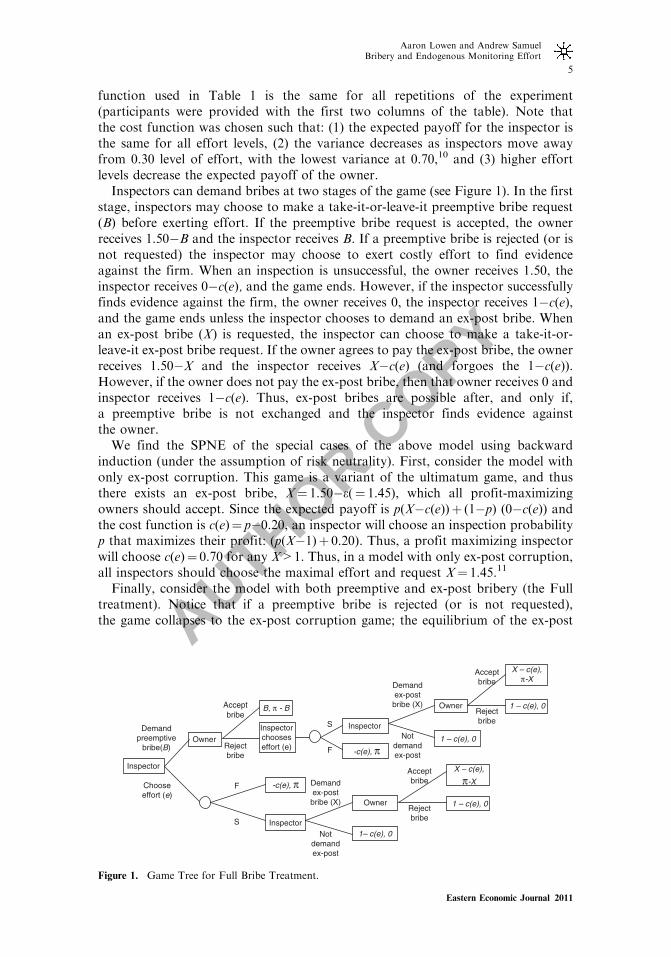
Inspectors can demand bribes at two stages of the game (see Figure 1). In the firststage, inspectors may choose to make a take-it-or-leave-it preemptive bribe request(B) before exerting effort. If the preemptive bribe request is accepted, the ownerreceives 1.50�B and the inspector receives B. If a preemptive bribe is rejected (or isnot requested) the inspector may choose to exert costly effort to find evidenceagainst the firm. When an inspection is unsuccessful, the owner receives 1.50, theinspector receives 0�c(e), and the game ends. However, if the inspector successfullyfinds evidence against the firm, the owner receives 0, the inspector receives 1�c(e),and the game ends unless the inspector chooses to demand an ex-post bribe. Whenan ex-post bribe (X) is requested, the inspector can choose to make a take-it-or-leave-it ex-post bribe request. If the owner agrees to pay the ex-post bribe, the ownerreceives 1.50�X and the inspector receives X�c(e) (and forgoes the 1�c(e)).However, if the owner does not pay the ex-post bribe, then that owner receives 0 andinspector receives 1�c(e). Thus, ex-post bribes are possible after, and only if,a preemptive bribe is not exchanged and the inspector finds evidence againstthe owner.

We find the SPNE of the special cases of the above model using backwardinduction (under the assumption of risk neutrality). First, consider the model withonly ex-post corruption. This game is a variant of the ultimatum game, and thusthere exists an ex-post bribe, X¼ 1.50�e(¼ 1.45), which all profit-maximizingowners should accept. Since the expected payoff is p(X�c(e))þ (1�p) (0�c(e)) andthe cost function is c(e)¼ p�0.20, an inspector will choose an inspection probabilityp that maximizes their profit: (p(X�1)þ 0.20). Thus, a profit maximizing inspectorwill choose c(e)¼ 0.70 for any X>1. Thus, in a model with only ex-post corruption,all inspectors should choose the maximal effort and request X¼ 1.45.11

Finally, consider the model with both preemptive and ex-post bribery (the Fulltreatment). Notice that if a preemptive bribe is rejected (or is not requested),the game collapses to the ex-post corruption game; the equilibrium of the ex-post

1 – c(e), 0

1 – c(e), 0

Acceptbribe

Rejectbribe

-c(e), π

S

F

Inspector

Demandex-postbribe (X)

Notdemandex-post

Owner

Demandpreemptive

bribe(B)

Inspector

Chooseeffort (e)

Owner

B, π - B

Inspectorchooseseffort (e)

Acceptbribe

Rejectbribe

S

-c(e), πF

Inspector

Demandex-postbribe (X) Owner

1– c(e), 0Notdemandex-post

Acceptbribe

Rejectbribe

X – c(e),

π-X

1 – c(e), 0

X – c(e),π-X

Figure 1. Game Tree for Full Bribe Treatment.


5


AUTHOR COPY

sub-game is the equilibrium of the game with only ex-post corruption (whereinspectors choose the maximal effort, c(e)¼ 0.70 and X¼ 1.45). Given this, in thepreemptive stage, the owner will agree to pay any preemptive bribe that is less thanthe expected value of X, B¼ 0.90 (1.45)�e(¼ 1.30).

It should be noted that two other solution concepts besides SPNE, “deal-me-out”and “split-the-difference” [Binmore et al. 1989; Oosterbeek et al. 1998], may berelevant here. Deal-me-out is a solution to a bargaining game where two partiessplit the surplus equally unless this gives one party less than their outside option.This is equivalent to saying the outside option does not affect bargaining powerexcept that it bounds the minimum acceptable offers. Within the context of ex-postbribery, splitting the 1.50 yields 1þ e(¼ 1.05) for the inspector (since his outsideoption is 1.00) and 0.45 for the owner. In contrast, split-the-difference assumes theoutside option affects the bargaining power, with the parties splitting the surplusremaining after both parties receive their outside option. Here, the inspector wouldreceive 1.25 and the owner 0.25. Although these solution concepts are based inthe result of back-and-forth negotiations, they could also embody different norms ofsharing, reciprocity, or fairness.12

Design choices

It is important to recognize seven important design choices regarding the abovemodel. First, all owners are guilty, and this is common knowledge (or, at least,public knowledge) among the participants. In the absence of this feature guiltyowners could reject bribe demands in order to falsely signal their innocence.Although interesting, this is likely to confound our findings because it introducesan additional level of uncertainty by requiring subjects to solve compound lotteries.Moreover, this imposition of guilt also avoids extortion (false claims of ownerguilt by inspectors). Finally, this experimental setting captures many realenvironments. For example, in the 1970s, Hong Kong’s police received bribesfrom known drug traffickers and owners of prostitution rings in exchange for notpursuing investigations [Klitgaard 1988]. This design choice is not without cost; itmay alter norms of reciprocity when participants are choosing bribe demands andchoices of inspection effort relative to the case where violations are determinedendogenously.

Our second fundamental design choice is to perfectly enforce the bribery contractbetween the players, eliminating the hold-up problem (such as when inspectorsdemand additional bribes). Incorporating hold-up creates an additional level ofuncertainty that complicates the game and confounds the effects of timing(preemptive vs ex-post). Thus, we enforce the collusive contract as in the briberyexperiments of Schulze and Frank [2003].

Our third design choice was to not implement a negative spillover as is the casein some bribery experiments. Omitting the externality had the benefit of simplifyingthe description and implementation of the payoffs for the participants. Thisalso helps isolate the role of the timing of bribes since reciprocal relationshipsare complicated; although participants may avoid creating spillovers out of a senseof fairness or altruism, they may choose to reciprocate negatively, anticipatingspillovers from other pairings. The role of these externalities in bribery experimentswas investigated by Abbink et al. [2002] and more recently by Castro [2011], whofind no detectable effect of an externality in a bribery experiment designed to testthis question. Similarly, Guth and van Damme [1998] implemented an ultimatum


6


AUTHOR COPY

game where an inert third party received a portion of the payoffs. The payoffs tothis third party, while not strictly an externality, were essentially minimized by theother two players. Even in the absence of these results, it is not clear that a corruptofficial would internalize an externality as would a participant from the generalpopulation, which would cause our subjects to behave in ways inconsistent withcorrupt officials.13

Our fourth design choice was to use in-context (loaded) language in ourinstructions. Abbink and Hennig-Schmidt [2006] find that context-free (neutral) vsin-context language created no difference in participant behavior. Similarly,Lambsdorff and Frank [2007] found that agent decision-making was notsignificantly affected by framing a bribe as a bribe vs gift-giving. Barr et al. [2004]find the mean behavior to be the same depending on the framing, but that there is asignificant increase in variance. Thus, given the likelihood of framing not affectingparticipant behaviors, and the increase in understanding from giving instructionsin-context, we use language such as “owner,” “inspector,” and “bribe.”

Fifth, we prevent explicit threats, intimidation, and coordination by imposinganonymity within each treatment and session and preventing extra-game commu-nication. Allowing these relationships might make the game more “realistic”but would make the data difficult to interpret. Attempting to evaluate the impactof this type of communication would be speculative at best. Further, allowingthis type of behavior would create anxiety and the potential for physical or otherharm to the participants. That said, threats and intimidation contribute to theexistence and magnitude of bribes beyond the inherent power held by bureaucrats.In our case, allowing owners to threaten inspectors would likely result in lessfrequent (and lower) bribe demands by inspectors, and lower effort exerted ininspection. Allowing inspectors to threaten owners would likely result in morefrequent (and higher) bribe demands by inspectors, and more bribes paid byowners.

We also chose to focus on the one-shot game to isolate the effects of the timingof bribery and minimize the confounding effects of reputation and learning aboutindividual partners. Finally, we chose to implement inspection costs as monetaryrather than as a real effort task. Given our interest in understanding the differentissues associated with preemptive vs ex-post bribery, we believe that thesesimplifying features are justified.

EXPERIMENTAL PARAMETERS AND PROCEDURES

A total of 80 subjects (four sessions of 20 each) participated in an inspector–ownerexperiment with real monetary stakes. Participants were randomly selected from apool of volunteers who responded to posters distributed across the campusesand announcements in a wide variety of classes (economics, classics, engineering,mathematics, political science, and general education courses). As a result,participants were drawn from a wide variety of majors at two regional Midwesternuniversities from October 2006 to April 2008. We did not track the Universityof origin of participants, but kept a list to make sure each participated at mostonce. The recruiting process did not provide the topic of the experiment but didindicate participants would receive a show-up fee of $8.

We took a number of steps to ensure that participants knew they were beingpaired with real players. First, participants were immediately and randomly sorted


7


AUTHOR COPY

into two rooms as they arrived. This separation had the added benefit of preventingcommunication between inspectors and owners. Talking was kept to a minimumwithin rooms. Second, sessions were held in adjoining rooms (separated by a partialwall) so identical verbal instructions could be given simultaneously to both rooms bya single experimenter, supplemented by paper copies. Finally, paper recording-formswere passed between rooms by the experimenters to allow participants to see thatanother player had filled out the form. A concern with communication of this sort isextra-game messages (reputation-building or threats) would substantially changethe game intended. To limit communication to that permitted by the model theinstructions included a warning that messages written on the forms wouldbe penalized by canceling any gains in the round of offense; none occurred.Instructions (including time for questions from participants), practice rounds(typically two per treatment), treatments, and distributions of cash payments tookslightly less than 90minutes in each session.

We also chose to implement our game as a series of one-shot interactions, ratherthan as a repeated game within pairs. This was done in an effort to minimizeboth the effects of reputation and the reciprocity of multi-period interactionsbetween a pair of players. Further, inspector identification codes were changedbetween treatments to reduce the possibility of reputation formation or reciprocalrelationships. Similar to Duffy and Feltovich [2006], we paired owners andinspectors on a “turnpike,”14 where no participant played another more than oncein a treatment. Participants were informed that they would be paired with a differentparticipant in each round within a treatment, and that their identificationcode would be changed between treatments. We then stated that this meant therewas no chance to build a reputation with any other participant, or to trade favors orpunishments either within the experiment or afterward. All players were allowed tokeep their recording forms from all treatments that included their previous partners’identification codes, offers, responses, and outcomes, but we did not observe anyplayers reviewing reporting forms from previous play.

Every session began with five rounds15 of a treatment without bribery (theNo-Bribe treatment). Both inspectors and owners were provided with instructionsthat included the cost of effort and chance of finding evidence information fromTable 1 (all players had access to this information in all rounds of all treatments).Owners and inspectors were paired. Inspectors then chose and recorded their cost ofeffort. Two ten-sided dice were then publicly rolled to create a percent value thatdetermined whether evidence was found against owners. The result of a single roll ofthe dice was applied to all inspectors. Both inspectors and their paired ownerswere informed of their outcome and both players recorded their payoffs (paid atthe end of the experiment). Owners and inspectors were matched with a new partnereach round.

The No-Bribery treatment was implemented for two reasons. First, observingeffort choice by inspectors, in the absence of bribery, reveals the net effect of riskand other-regarding attitudes on the effort choice by inspectors — in the absence ofbribery. Second, feedback from a pilot session indicated that the bribery taskswere sufficiently complicated (for inspectors) to warrant isolating the inspectionprocess. Thus, we do not follow the typical procedure of alternating the order of thetreatments across sessions. This deviation may introduce bias that limits the validityof the experiment. Since participants were first shown the bribe-free inspectionenvironment, they may perceive bribes as less socially acceptable or interpret thetreatment as either a benchmark or behavioral expectation from the experimenters.


8


AUTHOR COPY

Inspectors may have thus been influenced to ask for lower bribes, whereas ownersconditioned to expect a bribe-free environment. Both of these effects would bias theresults toward lower bribe demands and tougher owner standards (furtherexacerbating the strategic considerations by inspectors).

In addition to the No-Bribe treatment, every session included one or more of thefollowing bribery treatments: (1) the Preemptive bribe treatment, (2) the Ex-Postbribe treatment, and (3) the Full treatment, each corresponding to the games withonly preemptive bribery, only ex-post bribery, and both preemptive and ex-postbribery.16 The No-Bribe practice treatments were always conducted first, followedby the Preemptive or Ex-Post treatment, and finally by the Full treatment (ifapplicable). For clarity in the text we refer to the two sessions of the Ex-Posttreatment as sessions 1 and 2, although the Full are referred to as sessions 3 and 4.Sessions with the Full treatment were always preceded by five rounds of aPreemptive bribe treatment. We note this complicates the interpretation of ourresults by adding both extra history (albeit anonymous since we assigned newidentification numbers after each treatment) and a learning opportunity forparticipants in the Full treatment. The reason for this was feedback receivedfrom a pilot session, where participants indicated the preemptive section was a morecomplicated task than the ex-post.

In all sessions and for every round all players had access to the first two columnsof Table 1 and the public dice rolls, and were informed of their payoffs at the end ofthe round. In the Ex-Post and Full treatments only “honest” ex-post bribe demandswere allowed; only those inspectors who found evidence were allowed to request anex-post bribe, and owners were aware of this constraint. In the ex-post-only and Fulltreatments, the ex-post bribe demand forms contained the effort level exerted bythe inspector so the owner could confirm the inspector had found evidence againstthem. Similarly, an accepted bribe in the Preemptive and Full treatments endedthe round for the pair; no inspection or ex-post bribes were allowed once apreemptive bribe was accepted. All sessions were “yoked” in that players were onlyinformed about the current treatment, and a participant in the No-Bribe treatmenthad no reasonable expectation that an upcoming treatment would involve aparticular type of bribery (Preemptive, Ex-Post, or Full).

HYPOTHESES AND INFORMAL CONJECTURES

Given the SPNE predictions derived in the second section, we conjecture thatbehavior in the bribery treatments will be consistent with the following hypotheses.

Ex-Post bribe treatment

In treatments with only ex-post bribery, we conjecture the following:

Hypothesis 1: The ex-post bribe is equal to 1.45.17

Hypothesis 2: Inspectors exert the maximum effort (0.70) in the Ex-Post briberytreatment.

Hypothesis 3: The ex-post bribe demand is independent of the cost of effort.


9


AUTHOR COPY

Hypothesis 4(a): Owners pay all ex-post bribe requests Xp1.45.

Hypothesis 4(b): The likelihood of rejecting a bribe is increasing in the size ofthe bribe.18

Full treatment

Given the range of SPNE possible in the preemptive-only treatment, there are fewsharp predictions to be made in those treatments. Indeed, even theoretical modelsthat study preemptive bribery are able to derive clear predictions only by makingrather strong assumptions. Thus, we conjecture the following:

Hypothesis 5: Inspector effort in the Full treatment is 0.70.

Hypothesis 6: The preemptive bribe requested in the Full treatment is centeredon 1.30.

Hypothesis 7: The ex-post bribe requested in the Full treatment is centeredon 1.45.

Hypothesis 8: Owners are more likely to accept a preemptive bribe in the Fulltreatment than in the Preemptive treatment (after controlling for the size ofthe bribe).

It should be noted that Hypothesis 8 is not strictly a Nash prediction. However, dueto increased bargaining power, the preemptive bribe demand in the Full treatmentmust always be (weakly) greater than the preemptive bribe in the Preemptivetreatment. Thus, if the size of the bribe was the only factor that determined thedecision to pay a bribe, then owners should be no more likely to accept a preemptivebribe demand in the Full treatment than in the Preemptive treatment. However, ifowners expect inspectors to exert extra effort after a rejected preemptive bribedemand, then they will be more likely to accept a preemptive bribe in the Fulltreatment than in the Preemptive treatment.

RESULTS AND ANALYSIS

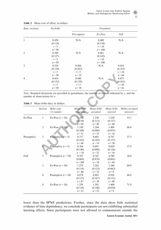
Descriptive statistics of the mean cost of effort are provided in Table 2, withmean bribe data in Table 3. Both Tables present descriptive statistics treatingeach choice by each player as an independent observation, but our analyses of thedata account for the dependent nature of the data (described below). The firstcolumn of Figure 2 contains the 75th and 25th quartiles (dashed lines) and medians(solid lines) of inspector Cost of Effort, and the second column contains inspectorBribe Requests by treatment, session, and round. Note that rounds 1 through 5 arethe No-Bribe treatment for all sessions, then are numbered following treatmentsas shown in Table 2 and the section “Experimental Parameters and Procedures.”Both preemptive and ex-post bribe requests are provided, with the ex-postbeing above one and the preemptive below one. We note that risk averse inspectorswould choose an effort level of 0.70 in all treatments, which rarely occurs in thedata. On average, ex-post bribe demands and inspection effort are significantly


10


AUTHOR COPY

lower than the SPNE predictions. Further, since the data show little statisticalevidence of time dependency, we conclude participants are not exhibiting substantiallearning effects. Since participants were not allowed to communicate outside the

Table 2 Mean cost of effort, in dollars

Date (session) No-bribe Treatment

Pre-emptive Ex-Post Full

1 0.450 N/A 0.480 N/A

(0.118) (0.134)

r=5 r=10

n=50 n=100

2 0.398 N/A 0.461 N/A

(0.127) (0.143)

r=5 r=10

n=50 n=100

3 0.356 0.466 N/A 0.418

(0.134) (0.203) (0.183)

r=5 r=5 r=10

n=50 n=32 n=66

4 0.416 0.446 N/A 0.475

(0.133) (0.129) (0.182)

r=5 r=5 r=10

n=50 n=28 n=61

Note: Standard deviations are provided in parentheses, the number of rounds indicated by r, and the

number of observations by n.

Table 3 Mean bribe data, in dollars

Session Bribe type

(# rounds)

Mean bribe

requested

Mean bribe

accepted

Mean bribe

rejected

Bribes accepted

(percent)

Ex-Post 1 Ex-Post (r=10) 1.182 1.150 1.220 55.1

(0.139) (0.113) (0.157)

n=89 n=49 n=40

2 Ex-Post (r=10) 1.330 1.294 1.409 68.6

(0.100) (0.096) (0.055)

n=51 n=35 n=16

Preemptive 3 Preemptive (r=5) 0.717 0.603 0.787 37.5

(0.165) (0.105) (0.157)

n=48 n=18 n=30

4 Preemptive (r=5) 0.766 0.691 0.869 57.9

(0.140) (0.098) (0.126)

n =38 n=22 n=16

Full 3 Preemptive (r=10) 0.767 0.741 0.780 34.0

(0.069) (0.078) (0.061)

n=100 n=34 n=66

3 Ex-Post (r=10) 1.279 1.263 1.344 80.0

(0.118) (0.123) (0.062)

n=40 n=32 n=8

4 Preemptive (r=10) 0.878 0.805 0.936 44.8

(0.127) (0.107) (0.112)

n=87 n=39 n=48

4 Ex-Post (r=10) 1.258 1.202 1.400 71.9

(0.156) (0.148) (0.050)

n=32 n=23 n=9


11


AUTHOR COPY

structure provided, we conclude that explicit threats, intimidation, or coordinationwithin player roles are unlikely explanations for their behavior.

Our experiment implements multiple one-shot games, making each inspector–owner pairing unique. However, turnpike matching can introduce intra-panel serialcorrelation, making each panel of 100 pairings a single independent observation.

Cost of Effort

Session1

Session2

Session3

Session4

00.10.20.30.40.50.60.70.80.9

1

00.10.20.30.40.50.60.70.80.9

1

00.10.20.30.40.50.60.70.80.9

1

0

0.1

0.2

0.3

0.4

0.5

0.6

0.7

0.8

0.9

1

Cos

t of E

ffort

1 2 3 4 5 6 7 8 9 10 11 12 13 14 15

1 2 3 4 5 6 7 8 9 10 11 12 13 14 15

1 2 3 4 5 6 7 8 9 10 11 12 13 14 15 16 17 18 19 20 1 2 3 4 5 6 7 8 9 10 11 12 13 14 15 16 17 18 19 20

Round

1 2 3 4 5 6 7 8 9 10 11 12 13 14 15Round

1 2 3 4 5 6 7 8 9 10 11 12 13 14 15

Round

0

0.25

0.5

0.75

1

1.25

1.5

0

0.25

0.5

0.75

1

1.25

1.5

0

0.25

0.5

0.75

1

1.25

1.5

0

0.25

0.5

0.75

1

1.25

1.5

Brib

e R

eque

st

Cos

t of E

ffort

Round

Brib

e R

eque

st

Cos

t of E

ffort

Round

Brib

e R

eque

st

Round

Cos

t of E

ffort

1 2 3 4 5 6 7 8 9 10 11 12 13 14 15 16 17 18 19 20

Round

1 2 3 4 5 6 7 8 9 10 11 12 13 14 15 16 17 18 19 20

Round

Brib

e R

eque

st

Bribe Request

Figure 2. Median Cost of Effort and Bribe Request, by Session.

Note: Solid lines show the median value in each round, with dashed lines the 75th and 25th percentiles.

Participants who have ended the round through failed inspection or accepted bribes are omitted. Bribe

Request graphs for sessions 3 and 4 include both preemptive bribes (lower sets of three lines) and ex-post

bribes (upper sets of three lines).


12


AUTHOR COPY

In order to draw more robust conclusions, we run each regression using differentpartitions of the data. First, we examine individual sessions (pooling participant-roundswithin each session). Second, we examine all participant-rounds fromthe same treatment pooled together. Third, we attempt to minimize the effects ofthis interdependence by pooling only the first round data of all participants fromidentical relevant treatment sessions. Using Round 1 data has the advantage ofreducing learning and reputation effects of later rounds, but suffers from fewerdata points and may still include effects by participants to “train” or createreputation for future rounds (see the discussion in footnote 14). Further, sincethere were five rounds of the No-Bribe treatment, these may be dependent onthose rounds as well.

Similar to Duffy and Feltovich [2006], we use random effects logit regressionswith controls for round to reduce potential bias from intra-panel serial correlation.Further, since pairings of participants are not independent, we extend our randomeffects models by using a Hierarchical Linear Model (HLM) where clusters arenested [Bryk and Raudenbush 1992; Cameron and Trivedi 2005; Rabe-Heskethand Skrondal 2008]. Our data have nested clusters, with round the lowest level ofobservation, followed by participant, and with session as the highest level.19

The simplest possible HLM (sometimes referred to as a variance componentsmodel) estimates the mean response (e.g. mean bribe requested and mean cost ofeffort) while allowing for dependence or correlation among the responses forobservations belonging to the same cluster [Bryk and Raudenbush, 1992, p. 17 ff].The maximum likelihood estimator of this model is a weighted mean of the clustermeans and may be used to make inferences for the mean.20 When estimatingrelationships (e.g. between bribe requests and the cost of effort) HLM may beinterpreted as an extension of random intercept models that also allows slopes of theindependent variables to vary randomly over clusters (in addition to the intercepts).This effectively relaxes the assumption that the dependent variable across all clustershas the same relationship with the independent variable (such as cost of effort).

We use the Stata 10 implementation of HLM through the command xtmixed toestimate all hierarchical models. We estimate the relationship between briberesponses and the size of the ex-post bribe demand using a HLM logit specificationfor binary responses, implemented in Stata 10 via xtmelogit.

Ex-Post bribe treatment

To test Hypotheses 1, 2, 5, 6, and 7, we conducted one-tailed z-tests using the(cluster corrected) standard errors from the HLM estimates (see Table 4). The testresults reject Hypothesis 1, that the ex-post bribe is equal to 1.45 (P-value o0.01).They also reject Hypothesis 2, that the cost of effort is equal to 0.70 (P-valueo0.01). If we follow the interpretation of each session being a single independentobservation we would compare the mean of each of the four sessions against 1.45.A Wilcoxon test under this set of assumptions results in a P-value of 0.0625(the lowest P-value possible with four observations), rejecting Hypothesis 1.Similarly, use of these four observations and the Wilcoxon test reject the cost ofeffort being equal to 0.70 (Hypothesis 2), also with a P-value of 0.0625. We alsoexamine whether inspectors treat the inspection cost as “sunk” when makingbribe requests (Hypothesis 3). We test this hypothesis by estimating a random effectsmodel (by inspector) in which the dependent variable is the dollar value of theex-post bribe request and the independent variables are the cost of effort and round,


13


AUTHOR COPY

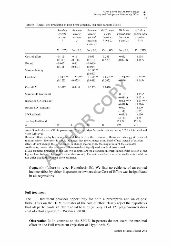
with results presented in Table 5. Our extended random effects specification (HLM)allows both the intercept and the slope to randomly vary by inspector and session.As discussed previously, we present results of each session separately, pooledtogether, and the first round of play (Round 1 only) from both sessions pooledtogether. In every specification, the data show no relationship between the cost ofeffort exerted and the size of the ex-post bribe requested by the inspector. Thus, wefind no evidence that inspectors condition ex-post bribe requests on their (sunk)inspection costs.

These results are summarized in Observation 1:

Observation 1: Inspectors request significantly lower ex-post bribes and exert lesseffort than is predicted by the SPNE (rejection of Hypotheses 1 and 2). However,inspectors treat effort costs as sunk when determining the size of their ex-postbribe (failure to reject Hypothesis 3).

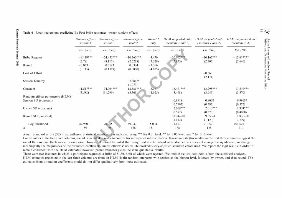
We also examine the decision of owners to accept or reject ex-post bribes. To studyowner behavior, we estimate a logit model (also random effects) where thedependent variable is the owner’s binary decision whether to pay an ex-post bribedemand, and the independent variables are the size of the bribe and the round(presented in Table 6). We also extend this random effects (logit) model to allow forrandom coefficients using an HLM specification.21 The HLM specificationessentially produces the same results as the random intercept model: the probabilityof accepting a bribe is significant and decreasing in the size of the bribe.22 Thus, notsurprisingly, larger bribe requests were more likely to be rejected, with no significanteffect by round (the pooled round one-only data show no relationship, but this isbecause only two of 15 bribe requests were rejected). We interpret the negative andstatistically significant estimated coefficient on Bribe Request to be evidence againstthe hypothesis that participants will pay any ex-post bribe less than or equal to 1.45(Hypothesis 4a).

The next-to-last column of Table 6 repeats this regression including theinspector’s Cost of Effort as an independent variable; if owners were able toobserve the inspector’s effort level they may have responded differently to higheffort inspections (the “earned income effect”). We see no evidence of this effecteither by inspectors (Table 5) or by owners (Table 6), since the Cost of Effort wasnot significant in either.

Observation 2: Owners frequently reject ex-post bribes that are substantiallylower than 1.45 (rejection of Hypothesis 4a), and reject larger bribe requests more

Table 4 HLM estimates for hypotheses 1, 2, 5, 6, and 7

Hypothesis 1 Hypothesis 2 Hypothesis 5 Hypothesis 6 Hypothesis 7

Ex-post bribe Cost of effort Cost of effort Preemptive bribe Ex-post bribe

Estimates 1.254*** 0.4705*** 0.444*** 0.8205*** 1.266***

(0.0541) (0.0256) (0.0350) (0.0383) (0.0236)

N 140 200 127 187 72

Note: Standard errors (SE) in parentheses. Statistical significance is indicated using *** for 0.01 level.

HLM estimates are for a random intercept model (with session at the highest level followed by inspector

and then round). We conduct z-tests based on the HLM estimates and standard errors.


14


AUTHOR COPY

frequently (failure to reject Hypothesis 4b). We find no evidence of an earnedincome effect by either inspectors or owners since Cost of Effort was insignificantin all regressions.

Full treatment

The Full treatment provides opportunity for both a preemptive and an ex-postbribe. Tests on the HLM estimates of the cost of effort clearly reject the hypothesisthat all participants set effort equal to 0.70 (in only 23 of 127 player-rounds doescost of effort equal 0.70; P-values o0.01).

Observation 3: In contrast to the SPNE, inspectors do not exert the maximaleffort in the Full treatment (rejection of Hypothesis 5).

Table 5 Regressions predicting ex-post bribe demands, inspector random effects

Random

effects

session

1

Random

effects

session

2

Random

effects

pooled

(sessions

1 and 2)

OLS round

1 only

(sessions

1 and 2)

HLM on

pooled data

(sessions

1 and 2)

HLM on

pooled data

(sessions

1–4)

Est. (SE) Est. (SE) Est. (SE) Est. (SE) Est. (SE) Est. (SE)

Cost of effort �0.115 0.161 0.033 0.365 0.033 0.004

(0.180) (0.130) (0.110) (0.570) (0.0978) (0.067)

Round �0.002 0.001 �0.0004(0.35) (0.003) (0.003)

Session dummy 0.154***

(0.050)

Constant 1.243*** 1.253*** 1.164*** 1.052*** 1.230*** 1.25***

(0.123) (0.073) (0.081) (0.305) (0.090) (0.045)

Overall R2 0.1017 0.0850 0.2363 0.0470

Session SD (constant) 0.103 0.055*

(0.0811) (0.031)

Inspector SD (constant) 0.0987*** 0.097***

(0.0184) (0.014)

Round SD (constant) 0.073 0.079

(1.51) (1.75)

SD[Residual] 0.0352 0.036

(3.144) (3.78)

— Log likelihood 125.24 171.04

N 89 51 140 15 140 211

Note: Standard errors (SE) in parentheses. Statistical significance is indicated using *** for 0.01 level and

* for 0.10 level.

Random effects are by Inspector (for models in the first three columns). Hausman tests suggest the use of

random effects. However, it should be noted that the estimates using fixed effects instead of random

effects do not change the significance, or change meaningfully the magnitudes of the estimated

coefficients, unless otherwise noted. Heteroskedasticity-adjusted standard errors used.

HLM estimates presented in the last two columns are for a random intercept model (with session at the

highest level followed by inspector and then round). The estimates from a random coefficients model do

not differ qualitatively from these estimates.


15


AUTHOR COPY

Table 6 Logit regressions predicting Ex-Post bribe-responses, owner random effects

Random effects

session 1

Random effects

session 2

Random effects

pooled

Round 1

only

HLM on pooled data

(sessions 1 and 2)

HLM on pooled data

(sessions 1 and 2)

HLM on pooled data

(sessions 1–4)

Est. (SE) Est. (SE) Est. (SE) Est. (SE) Est. (SE) Est. (SE) Est. (SE)

Bribe Request �9.119*** �24.455*** �10.360*** 4.470 �10.002*** �10.162*** �12.619***(2.78) (8.117) (2.6218) (3.529) (2.635) (2.707) (2.646)

Round �0.033 0.0193 0.0324 �3.366(0.115) (0.1319) (0.0880) (4.025)

Cost of Effort �0.663(2.174)

Session Dummy 2.384**

(1.073)

Constant 11.517*** 34.004*** 12.581*** �3.367 13.471*** 13.998*** 17.519***

(3.588) (11.299) (3.301) (4.025) (3.498) (3.945) (3.570)

Random effects parameters (HLM):

Session SD (constant) 0.8918 0.9008 0.9918*

(0.7902) (0.793) (0.575)

Owner SD (constant) 2.009*** 2.010*** 1.974***

(0.572) (0.573) (0.4800)

Round SD (constant) 8.74e–07 9.65e–11 1.81e–10

(1.112) (1.120) (.799)

— Log likelihood 42.960 20.385 69.047 5.034 71.103 71.057 101.621

N 89 49 138 15 138 138 210

Notes: Standard errors (SE) in parentheses. Statistical significance is indicated using *** for 0.01 level, ** for 0.05 level, and * for 0.10 level.

For estimates in the first three columns, round is included in order to control for intra-panel autocorrelation. Hausman tests (for models in the first three columns) suggest the

use of the random effects model in each case. However, it should be noted that using fixed effects instead of random effects does not change the significance, or change

meaningfully the magnitudes of the estimated coefficients, unless otherwise noted. Heteroskedasticity-adjusted standard errors used. We report the logit results in order to

remain consistent with the HLM estimates, however, probit estimates yields the same qualitative results.

There were two instances in which a participant requested a bribe of $1.50, both of which were rejected. We omit these two data points from the statistical analyses.

HLM estimates presented in the last three columns are from an HLM (logit) random intercepts with session as the highest level, followed by owner, and then round. The

estimates from a random coefficients model do not differ qualitatively from these estimates.

AaronLowen

andAndrew

Samuel

Brib

eryandEndogenousMonito

ringEffo

rt

16

Eastern

Economic

Journal2011

AUTHOR COPY

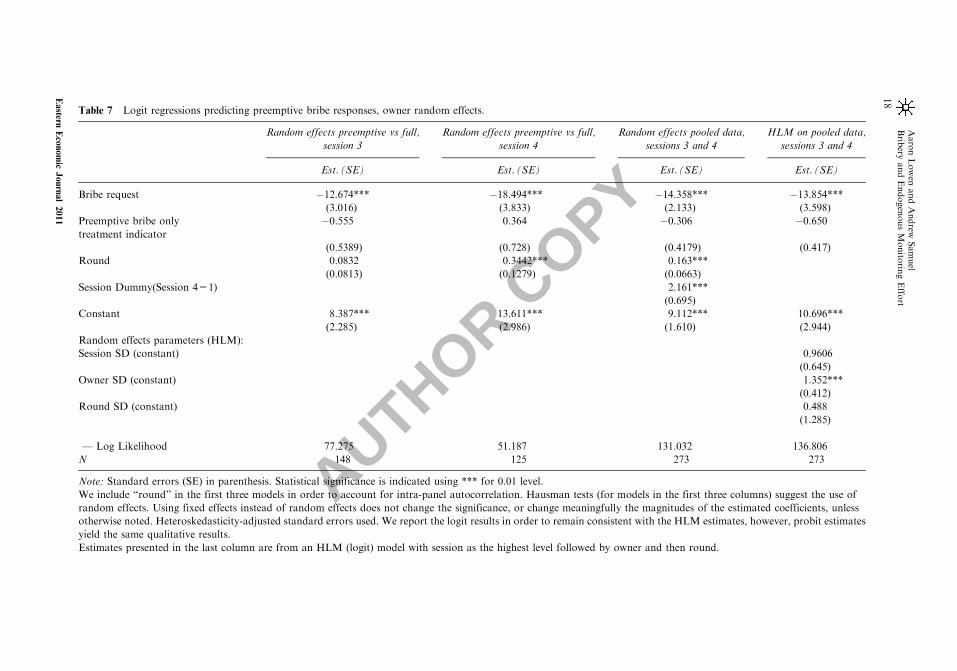
Hypothesis 6 states that the preemptive bribes in the Full treatment will be centeredon 1.30. Tests on the HLM estimates of the preemptive bribes in the Full treatment(see Table 4) reject the claim that the bribe requests in the Full treatment are equal to1.30 (all P-values o0.01). Similarly, Hypothesis 7 states that the ex-post bribes inthe Full treatment will be equal to 1.45. Tests on the HLM estimates reject that thebribe requests in the Full treatment are equal to 1.45 (P-value o0.01). Finally,Hypothesis 8 asserts that owners are less likely to accept a preemptive bribe inthe Full treatment than in the Preemptive treatment. We estimate a logit modelwith random effects, where the binary dependent variable is whether the ownerpays a preemptive bribe. In this model the independent variables are a treatmentdummy, the round, and the preemptive bribe requested (see Table 7). The data showthat, when controlling for the size of the bribe, the treatment dummy is insignificantin each model. In other words, the increased frequency in the rejection of bribedemands occurs because inspectors demand higher bribes, whereas owners respondthe same way given the size of the bribe demand. We summarize these findings inObservation 4.

Observation 4: The preemptive bribes demanded in the full treatment are notequal to the Nash prediction (rejection of Hypothesis 6). Similarly, the ex-postbribes demanded the Full treatments are significantly lower than the Nashprediction (rejection of Hypothesis 7). However, we find no evidence that ownersare more likely to reject a preemptive bribe in the Full treatment than in thePreemptive bribe treatment when controlling for the size of the bribe (rejectionof Hypothesis 8).

Alternative solution concepts

The deal-me-out and split-the-difference solution concepts are not good predictors ofparticipant behavior. Of the 212 total ex-post bribes across all treatments and sessions,25 (11.8 percent) were less than or equal to bribe offers of 1.05, indicating deal-me-outwas not a good descriptor of behavior. Similarly, 20 (9.4 percent) bribe offers wereequal to 1.25, indicating split-the-difference was not a good descriptor of behavioreither. The SPNE prediction fares about the same with 10 (4.7 percent) offers greaterthan or equal to 1.45. Since our experiment was not designed to distinguish betweenthese three bargaining solutions, we do not test these hypotheses more formally.

DISCUSSION OF RESULTS AND CONCLUSION

This paper presents the findings of a laboratory experiment based on a modelof bribery first developed in Mookherjee and Png [1995]. Despite a body oftheoretical research that extends this work, and an array of important policyapplications that have been drawn from this model, empirical analysis of thestrategies of players has not been undertaken because key variables are unobservable(such as cost of inspection effort). Our experimental evidence finds that the behaviorof participants deviates significantly from many of the sharper predictions ofMookherjee and Png [1995] and Samuel [2009]. Specifically, our data on ex-postbribery suggest that inspector behavior is inconsistent with the SPNE prediction. Inparticular, inspectors do not choose the payoff maximizing ex-post bribe(Observation 1). Similarly, in the Full treatment we find that the preemptive bribe


17


AUTHOR COPY

Table 7 Logit regressions predicting preemptive bribe responses, owner random effects.

Random effects preemptive vs full,

session 3

Random effects preemptive vs full,

session 4

Random effects pooled data,

sessions 3 and 4

HLM on pooled data,

sessions 3 and 4

Est. (SE) Est. (SE) Est. (SE) Est. (SE)

Bribe request �12.674*** �18.494*** �14.358*** �13.854***(3.016) (3.833) (2.133) (3.598)

Preemptive bribe only

treatment indicator

�0.555 0.364 �0.306 �0.650

(0.5389) (0.728) (0.4179) (0.417)

Round 0.0832 0.3442*** 0.163***

(0.0813) (0.1279) (0.0663)

Session Dummy(Session 4=1) 2.161***

(0.695)

Constant 8.387*** 13.611*** 9.112*** 10.696***

(2.285) (2.986) (1.610) (2.944)

Random effects parameters (HLM):

Session SD (constant) 0.9606

(0.645)

Owner SD (constant) 1.352***

(0.412)

Round SD (constant) 0.488

(1.285)

— Log Likelihood 77.275 51.187 131.032 136.806

N 148 125 273 273

Note: Standard errors (SE) in parenthesis. Statistical significance is indicated using *** for 0.01 level.

We include “round” in the first three models in order to account for intra-panel autocorrelation. Hausman tests (for models in the first three columns) suggest the use of

random effects. Using fixed effects instead of random effects does not change the significance, or change meaningfully the magnitudes of the estimated coefficients, unless

otherwise noted. Heteroskedasticity-adjusted standard errors used. We report the logit results in order to remain consistent with the HLM estimates, however, probit estimates

yield the same qualitative results.

Estimates presented in the last column are from an HLM (logit) model with session as the highest level followed by owner and then round.

AaronLowen

andAndrew

Samuel

Brib

eryandEndogenousMonito

ringEffo

rt

18

Eastern

Economic

Journal2011

AUTHOR COPY

(as well as the ex-post bribe) is significantly lower than the payoff-maximizing bribe(Observation 4). In light of the previously discussed experimental literature onthe ultimatum game, the result that inspectors do not demand the maximumbribe is not entirely surprising. Of particular importance is the fact that inspectorschoose not to demand the maximum bribe even though they had to earn the rightto extract this payoff from the owner. The earned income effect of Cherry et al.[2002] thus does not dominate the sharing norms common in ultimatum gameenvironments.

The result that reciprocity affects the size of bribes, even when inspectors mustexert costly effort to earn the right to extract them, has two policy implications.First, since owners are always more likely to accept lower bribes, these normsmay actually support bribery. Second, this result sheds light on whether bribescan be used as a substitute for a legal penalty. The literature on corruption arguesthat, when the inspector has all the bargaining power, the bribe and the fine areequivalent because the inspector can extract almost the entire fine in the form ofa bribe [Becker and Stigler 1974; Polinsky and Shavell 2001]. Indeed, ex-postbribery can be shown to be socially optimal if the inspector has all the bargainingpower (see Mookherjee and Png [1995, footnote 27]). In light of these theoreticalresults, our finding that ex-post bribes are significantly lower than the fine isimportant. Specifically, even though the inspector has all the bargaining power inour game, sharing norms limit the size of the bribe to be considerably lower thanthe fine. Thus, bribery is unlikely to provide as strong a deterrent as the fine.Further, in reality the result that bribery is sometimes socially optimal (whichdepends on the assumption that the bribe is as large as the fine) is not likely to beapplicable.

Our second finding, described in Observation 1 and Observation 3, is thatinspectors do not exert the payoff maximizing level of effort (in the sense that itmaximizes the probability of an ex-post bribe). To our knowledge this behavior isnew to the corruption literature. The finding that inspectors do not exert payoff-maximizing effort under ex-post bribery has important implications for evaluatingthe welfare costs of bribery. Previous theoretical research has shown that ex-postbribery can cause inspectors to exert too much effort because the bribe must belarger than the inspector’s reward. Thus, bribery can cause inspectors to exert toomuch effort, that is, more effort than is socially optimal [Mookherjee and Png 1995].Our data show that although ex-post bribery does incentivize inspection effort, thelevel of effort is not as high as that predicted by the Nash equilibrium. Thus,the inefficiencies caused by excessive effort under ex-post bribery may beameliorated by an inspector’s incentives for reciprocity.

Third, owner responses to ex-post bribe demands are similar to responderbehaviors in the ultimatum game [Camerer and Thaler 1995] (Observation 2).Namely, owners do not accept all offers, and frequently forego substantial monetarypayoffs by rejecting “reasonable” offers. Thus, owner behavior also providessupport for the role of sharing norms.

In light of these experiments, we believe that reciprocal behavior observed inthe behavioral literature (as discussed in Camerer and Thaler [1995]) appearswithin the context of corruption through sharing norms (as they relate tothe inspection process). As discussed above, such behavior can have an impact onthe policy implications and welfare impact of corruption. Thus, models ofcorruption will be more accurate if they incorporate such behavior explicitly intothe model.


19


AUTHOR COPY

Acknowledgements

We wish to thank three anonymous referees, Emmanuel Dechenaux, andChristopher Morrell, as well as seminar participants at the 2007 InternationalIndustrial Organization Conference and at the workshop on Law, Economics, andInstitutions — University of Birmingham (UK). Alden Van Slokema, AndrewVlietstra, and Laura Samuel provided excellent assistance in running ourexperiments. Financial support from the Calvin College Center for Social Research,Loyola University — Maryland, and Grand Valley State University is alsogratefully acknowledged.

APPENDIX

Instructions for the full bribe treatment

General informationYou are going to participate in an experiment that simulates an inspector–inspecteerelationship. These instructions explain how the decisions you and the otherparticipants make determine the total cash payment you will receive at the end ofthe session. During the session you must keep track of your payments on the formsprovided to you. At the end of the session, your total profits will be paid to you in cash.

BackgroundThe Department of Health has just instituted a new set of health code requirementsfor restaurants. All restaurant owners are currently in violation of these newhealth code requirements. The Department of Health has hired health inspectorsto investigate these restaurants. Inspectors must exert costly effort in order tocollect evidence against a restaurant owner. By exerting a higher degree of effortinspectors are able to find evidence of the owner’s guilt with greater probability.However, a higher degree of effort costs more than a lower degree of effort.This relationship between the inspector’s cost of effort is given by the followingtable:

For example, if an inspector incurs $0.20 of effort, that inspector will havea 40 percent chance of finding evidence (of health code violations) against the owner.

Each time an inspector successfully collects evidence against a restaurant, theinspector is paid $1minus the cost of effort. If the inspector does not successfully collectevidence, the inspector still pays the cost of effort whereas the owner is receives $1.50.

Cost of effort exerted Chance of finding evidence (%)

$0.00 20

$0.10 30

$0.20 40

$0.30 50

$0.40 60

$0.50 70

$0.60 80

$0.70 90


20


AUTHOR COPY

Your rolesYou have the same role assigned in the previous round, either an Owner or anInspector. As earlier, you will never know the identity of your partner for any round,and are matched in such a way that you will never play the same person twice inthis session.

Recording your payoffsAll inspectors must have a short form and an inspector’s long form and all ownersan owners’ long form. Please do NOT write down anything other than the requestedinformation (additional messages or comments will result in a penalty for the round).

The gameThe stages of the game take place in the following order:

Stage 1: Keeping in mind that no owners are in compliance with the health code, theinspector specifies a bribe amount (in 5 cent increments) that he/she is willing toaccept in exchange for not inspecting the restaurant. Inspectors may choose NOT torequest a bribe at this stage.Records: The inspector records this initial decision on the short and long forms. Theinspector is then matched with an owner who receives the inspector’s offer on the shortform. Please make sure to fill out all the information pertaining to the inspector on boththe short and the long forms.

Stage 2: The restaurant owner responds by either accepting or rejecting the bribe.Records: The owner records their choice on both the short and long forms.

Stage 3: If the owner accepts the bribe, the inspector does not exert any effort and theround ends. In this case the owner gets $1.50minus the bribe and the inspectorreceives the amount of the bribe. Inspectors will be informed if their bribe is rejected,and they will proceed to stage 4.Records: Owners and inspectors record their payoffs (if applicable) and actions on thelong form.

Stage 4: If the Inspector chose not to request a bribe in stage 1 or the inspector’sbribe was rejected in stage 2, the inspector must choose a level of effort and aprobability of finding evidence against a guilty owner, according to the above table.Once all inspectors have chosen their effort level a die is thrown.

If the die roll is equal to or below the inspectors’ chance of finding evidence, theinspector receives a payoff of $1minus the cost of effort. These inspectors have foundevidence against their corresponding restaurant owner and the corresponding ownerreceives a payoff of $0. Inspectors who find evidence against their assigned ownerwill be announced.

If the die roll is above the inspectors’ chance of finding evidence, the inspectorreceives a payoff of $0 but still incurs the cost of effort. These inspectors have notfound any evidence against their corresponding restaurant owner and the ownerreceives a payoff of $1.50. Note that it is possible to have negative profit for a round.Records: Inspectors record the outcome of the dice role on the “Inspection Outcome”column whether they found Evidence or No-evidence, and their earnings in that round.Owners record the result of the inspection and their earnings.


21


AUTHOR COPY

Stage 5: If the Inspector has found evidence (according to the outcome of the die rollin stage 4), he/she must specify a bribe amount that he/she is willing to acceptin exchange for not reporting the restaurant. Please realize that you may choose NOTto request a bribe at this stage.Records: ALL INSPECTORS, regardless of whether they have found evidence againstthe Owner, must fill out a bribe form. All inspectors must state their effort level andwhether he has found evidence or not found evidence. If no evidence has been found,Inspectors CANNOT request a bribe. However, if the evidence has been found,Inspectors may request a bribe, but do not have to.

Stage 6: Owners choose to accept or reject their Inspector’s bribe. If the bribe isaccepted the Owner receives $1.50minus the bribe paid and the Inspector receives thebribe minus the cost of effort. If the bribe is rejected, an owner receives $0 for thatround and the Inspector receives a payoff of $1minus the cost of effort.Records: Inspector–Owner pairs record their payoff on their long forms.

Are there any questions?

Notes

1. In their summary of the literature, Dusek et al. [2004] identify other social ills associated with high

rates of corruption and bribery such as: increased poverty rates and decreased foreign private

investment, economic growth rates, government revenues and infrastructure, and social equality.

2. See Samuel [2009] for a theoretical model of preemptive and ex-post bribery.

3. The most similar experiments that use endogenous effort are Dittrich and Kocher [2006] and Fehr

et al. [1997], but they examine the role of different wage contracts on employee effort. Specifically,

they find that, despite effort being non-contractible and unobservable in their experiment, workers

frequently exert effort that is above the payoff-maximizing level when they perceive that they will be

rewarded with higher wages (even when these higher wages are not guaranteed).

4. In real situations, agents may have to manage reputations or repeated play, but the basic structure is

still one of bargaining after sunk costs. We focus on the one-shot game instead of one of reputation or

repeated play in order to reflect Mookherjee and Png [1995] most closely.

5. As discussed in Lambsdorff and Frank [2007], the relevant “sharing norm” in a game of corruption is

reciprocity, not fairness. Whereas fairness indicates a sharing norm that would proscribe society-

harming corruption, reciprocity permits the provision of surplus gained from illegal behavior.

6. To illustrate, Abbink et al. [2002] also analyze bribery as a reciprocity game, but implement it

differently. In their game the first player offers a bribe to the second, who may reject the offer. The

second then chooses whether to create a large surplus for the first at a small personal cost. The game

features right of refusal, reneging, transfer fees, multiplication of transferred values, an exogenous

chance of being caught and punished, and externalities levied against other players. Given their

interest in long-term relationships, they implement 30-round sessions in which players have the same

partner in every round. Their results suggest that repeated interaction strengthens reciprocal behavior

in that first movers are more likely to transfer money (pay bribes) to second movers.

7. These experiments also find that when positive and negative reciprocity are observed in the lab,

negative reciprocity appears to occur more frequently.

8. Recognizing the challenges of using field data to understand bureaucrat behavior is not the same as

establishing the external validity of experiments on corrupt behaviors. As Abbink [2006] notes, the

standard use of students and the inherently artificial nature of experiments weakens their external

validity but are still an excellent way to test theoretical models (such as we do with Mookherjee and

Png [1995]). In response, Abbink notes that “y[field research] suffer[s] from the noise, identification

problems, and lack of control” (p. 1). Although not a direct test of external validity, Barr et al. [2004]

implement an embezzlement experiment with health workers, and their results generally support prior

experimental research on students, giving some empirical support for the external validity of

corruption experiments. Using potentially corrupt bureaucrats as participants has problems as well, as

they would be aware of being observed making choices about behaviors similar to their own illegal

activities and likely behave in contrived ways. Abbink [2006, p. 436] notes that “(a)lthough it is


22


AUTHOR COPY

naturally impossible to prove the external validity of experimental results, such parallel investigations

could dramatically add to the robustness of the stylized facts we can identify in laboratory

experiments.” Dusek et al. [2004] claim experiments are useful for designing incentive-compatible

and effective anti-corruption measures. The fact that real situations often feature indefinitely repeated

interactions indicates that more trust and reciprocity likely occur in real settings, and so experiments

would underestimate the extent of corruption. Knowing the direction of bias informs us how to

interpret experimental results, and thus they are still useful for analyzing public policy. For example,

they note that since college students seem to ignore spillovers onto other participants, the implication

is clear that corrupt bureaucrats would likely not either, and that moral suasion and ad campaigns

will be of little help. Further, if college students have trouble correctly using percentages of being

caught, respond to wage increases by decreasing corrupt behaviors, exhibit inequality aversion, and

respond to beliefs about the prevalence of corruption, we can safely assume bureaucrats and

bribe-payers likely exhibit these stylized behaviors as well. Thus, while experiments may not exhibit

external validity in the overall magnitude of bribery, they would be informative of underlying

behaviors.

9. In order to prevent the inspector from falsely accusing the owner, inspectors must present verifiable

evidence before they can collect a fine from the owner.

10. The choice with the lowest variance is 0.70, whereas the choice with the smallest potential loss is

0 cents. Thus, strongly risk-averse agents will always choose 0.70, whereas strongly loss-averse agents

will always choose 0 cents. In our experiments, however, we rarely see either.

11. Note bribe demands were in 0.05 increments. Although profit-maximizing owners would be indifferent

to a bribe request of 1.50, we assume (here) that inspectors would not offer a weakly dominated bribe

request.

12. We are grateful to an anonymous referee for raising these issues.

13. Although previous experimental research on bribery suggests an externality does not affect the

likelihood of bribes [Abbink et al. 2002], the presence of a negative externality (due to the firm’s

non-compliance) may encourage more intensive inspections if inspectors are empathetic or hold norms

of fairness. Such findings would also have implications for Harrington’s [1988] model of inspections

and firm compliance, and its experimental implementation in Cason and Gangadharan [2005].

14. We note there are limited design options available. Our approach introduces contagion, potentially

leaving potential for both training effects (an attempt to influence future partners indirectly through

choices against current partners) and reputation-building. Although we did not attempt to measure

the effects of this contamination, we believe the effects to be smaller than that from repeated pairings,

which maximize the incentives for training and reputation effects. Further, such a super-game would

neutralize the timing effect of bribery, as one period’s ex-post bribe would be directly followed by the

next period’s preemptive bribe. A third alternative would be to bring in participants for a single round

of play. Given the high cost of attracting participants and substantial time to give instructions, such

an approach was infeasible. In our econometric analysis below we analyze all rounds of data (using

HLM techniques), but as a robustness check also analyze only the first round of play. (See Harrison

[2007] for further caveats on examining only the first round of data).

15. Note that two practice rounds of each treatment were done without financial incentives to allow for

learning about the flow and structure of the treatment and questions. We recorded and report only

those rounds played for money. Participants were informed of the number of rounds of each treatment

verbally and through the format of their information-recording forms.

16. Instructions for the Full treatment are included in the Appendix.

17. Hypothesis 1 is one-tailed, with evidence against the hypothesis being bribes below 1.45; since

permissible bribes were in 0.05 increments, 1.45 is the largest bribe demand that gives the owner a

non-zero payoff.

18. Since we expect to observe some bribe demands being rejected, which is off-equilibrium path behavior,

we test for this hypothesis.

19. Cameron and Trivedi [2005] state that when the structure of the data consists of a short panel, this is

the correct way to model the hierarchical structure. We include session as a level in order to account

for possible session-level effects. However, our qualitative findings remain unchanged whether or not

session is included as a level in our HLM estimates.

20. The maximum likelihood estimator is preferred because it is more efficient and its standard error

is weakly greater than the Ordinary Least Squares (OLS) estimator. If one is not interested in the

within-cluster dependence, then the OLS “sandwich” estimator may also be used. This sandwich

estimator takes this clustering into account to produce “robust” standard errors [see Rabe-Hesketh

and Skrondal 2008, pp. 68 ff.]. For robustness we estimate our model using both estimators but only

present the HLM estimates. OLS results are included for comparison, and not discussed here.


23


AUTHOR COPY

Similarly, we pool the sessions at various levels (both identical sessions and all four sessions, when

applicable) and find no qualitative difference in our results.

21. This HLM specification allows for both random coefficients and slopes by owner and is effectively

an extension of a random effects logit model.

22. Since we are only interested in estimating and conducting hypothesis tests on the coefficients, we do

not discuss these variance estimates.

References

Abbink, K. 2006. Laboratory Experiments on Corruption, in International Handbook on the Economics of

Corruption, edited by S. Rose-Ackerman. Northampton, USA: Edward Elgar Publishing Limited,

418–437.

Abbink, K., B. Irlenbusch, and E. Renner. 2000. The Moonlighting Game: An Experimental Study on

Reciprocity and Retribution. Journal of Economic Behavior and Organization, 42: 265–277._______ . 2002. An Experimental Bribery Game. Journal of Law, Economics, and Organization, 18:

428–454.

Abbink, K., and H. Hennig-Schmidt. 2006. Neutral Versus Loaded Instructions in a Bribery Experiment.

Experimental Economics, 9: 103–121.

Bardhan, P. 2006. The Economist’s Approach to the Problem of Corruption. World Development, 34:

341–348.

Barr, A., M. Lindelow, and P. Serneels. 2004. To Serve the Community or Oneself: The Public Servant’s

Dilemma, World Bank Policy Research Working Paper 3187.

Becker, G., and G. Stigler. 1974. Law Enforcement, Malfeasance and Compensation of Enforcers. Journal

of Legal Studies, 3: 1–18.

Berg, J., J. Dickhaut, and K. McCabe. 1995. Trust, Reciprocity and Social History. Games and Economic

Behavior, 10: 122–142.

Binmore, K., A. Shaked, and J. Sutton. 1989. An Outside Option Experiment. The Quarterly Journal of

Economics, 104: 753–770.

Boycko, M., A. Shleifer, and R. Vishny. 1995. Privatizing Russia. Cambridge: MIT Press.

Bryk, A.S., and S.W. Raudenbush. 1992. Hierarchical Linear Models. California USA: Sage Publications.

Camerer, C., and R. Thaler. 1995. Anomalies: Ultimatums, Dictators and Manners. Journal of Economic

Perspectives, 9: 209–219.

Cameron, A., and P. Trivedi. 2005. Microeconomics: Methods and Applications. Cambridge: Cambridge

University Press.

Cason, T.N., and L. Gangadharan. 2005. An Experimental Study of Compliance and Leverage in

Auditing and Regulatory Enforcement. Economic Inquiry, 44: 352–366.

Castro, F.M. 2011. To Bribe or not to Bribe: An Experimental Analysis of Corruption, DSSGES

Working Paper, Universita Mediterranea di Reggio, Calabria.

Cherry, T., P. Frykblom, and J. Shogren. 2002. Hardnose the Dictator. American Economic Review, 92:

1218–1221.

Dittrich, D., and M. Kocher. 2006. Monitoring and Pay: An Experiment on Employee Performance under

Endogenous Supervision, CEPR Discussion Paper No. 5962.

Duffy, J., and N.J. Feltovich. 2006. Words, Deeds and Lies: Strategic Behavior in Games with Multiple

Signals. Review of Economic Studies, 73: 669–688.

Dusek, L., A. Ortmann, and L. Lizal. 2004. Understanding Corruption and Corruptibility Through

Experiments: A Primer, CERGE-EI Discussion Paper No. 2004 -136.

Fehr, E., S. Gachter, and G. Kirchsteiger. 1997. Reciprocity as a Contract Enforcement Device:

Experimental Evidence. Econometrica, 65: 833–860.

Greenhouse, S. 2008. School Bus Safety Officers are Accused of Soliciting Bribes, New York Times

(May 14).

Guth, W., and E. van Damme. 1998. Information, Strategic Behavior, and Fairness in Ultimatum

Bargaining: An Experimental Study. Journal of Mathematical Psychology, 42: 227–247.

Harrington, W. 1988. Enforcement Leverage when Penalties are Restricted. Journal of Public Economics,

37: 29–53.

Harrison, G. 2007. House Money Effects in Public Good Experiments: Comment. Experimental

Economics, 10: 429–437.

Hunt, J., and S. Laszlo. 2005. Bribery: Who Pays, Who Refuses, What are the Payoffs? NBER Working

Paper 11635.


24


AUTHOR COPY

Klitgaard, R. 1988. Controlling Corruption. Berkeley, CA: University of California Press.

Lambsdorff, J., and B. Frank. 2007. Corrupt Reciprocity — An Experiment, University of Passau

Discussion Paper V-51-07.

Lubin, N. 2003. Who’s Watching the Watchdogs? Journal of International Affairs, 56: 43–57.

Mookherjee, D., and I. Png. 1995. Corruptible Law Enforcers: How Should They Be Compensated? The

Economic Journal, 105: 145–159.

Olken, B., and P. Barron. 2007. The Simple Economics of Extortion: Evidence from Trucking in Aceh,

NBER Working Paper No. 13145, Cambridge: National Bureau of Economic Research.

Oosterbeek, H., J. Sonnemans, and S. vanVelzen. 1998. Bargaining with Endogenous Pie Size and

Disagreement Points; A Holdup Experiment, Working Paper.

Phillips, O., R. Battalio, and C. Kogut. 1991. Sunk and Opportunity Costs in Valuation and Bidding.

Southern Economic Journal, 58: 112–128.

Polinsky, A., and S. Shavell. 2001. Corruption and Optimal Law Enforcement. Journal of Public

Economics, 81: 1–24.

Rabe-Hesketh, S., and A. Skrondal. 2008. Multilevel and Longitudinal Modeling Using Stata, 2nd ed.,

College Station, TX: Stata Press.

Rubin, E. 2006. In the Land of the Taliban, New York Times Magazine, October 22: 91.

Samuel, A. 2009. Preemptive Collusion among Corruptible Law Enforcers. Journal of Economic Behavior

and Organization, 71: 441–450.

Schmitt, P. 2004. On perceptions of Fairness: The Role of Valuations, Outside Options, and Information

in Ultimatum Bargaining Games. Experimental Economics, 7: 49–73.

Schulze, G., and B. Frank. 2003. Deterrence Versus Intrinsic Motivation: Experimental Evidence on the

Determinants of Corruptibility. Economics of Governance, 4: 143–160.

Simpson, J., and Z. Bojovic. 2005. Investigation: Serbia Losing Customs Corruption Battle, Institute

for War and Peace Reporting, BCR No 541, 11-Feb-05.

Svensson, J. 2003. Who Must Pay Bribes and How Much? Evidence from a Cross Section of Firms. The

Quarterly Journal of Economics, 118: 207–230.


25


bribery and endogenous monitoring effort: an experimental...

Documents