breeden consumption as a leading indicator april 2012
TRANSCRIPT

Preliminary. Comments invited.
Consumption As A Leading Indicator
By
Douglas T. Breeden*
Current version: April 18, 2012 *Fischer Black Visiting Professor of Financial Economics at the Massachusetts Institute of Technology ([email protected]) and William W. Priest Professor of Finance and Former Dean, Fuqua School of Business, Duke University. I thank participants at seminars at Duke, North Carolina, Boston College, Boston University, University College Dublin, Ireland, the World Finance Conference in Rhodes, Greece, and Finance Down Under at Melbourne Business School. Special thanks go to Campbell Harvey for his extensive comments on an earlier version of this paper, to Duane Stock for his discussion in Greece and to John Payne for his help on behavioral research in decision making. I also thank Lina Ren, Jonathan Ashworth and Mark Breeden at Duke and LiAn Pan at MIT for their research assistance.

1
Abstract
This article shows that real, total consumption growth deviations from normal stock market
wealth effects lead economic growth. Consumers’ expenditures reflect their information about
employment opportunities and future real wage growth, as well as information about the
volatility of future investment returns. Previous research has shown that stock prices and the
slope of the term structure of interest rates reflect forecasted economic growth and profits. It is
shown that consumption deviations improve growth forecasts based upon the signals given by
the term structure and stock returns over the 50-year period from 1961 to 2011 and in the recent
(2006-2009) volatile period of rapid growth followed by financial panic. Putting the information
from the stock market, the bond market and consumers together, we find that all three key
variables are statistically significant in regressions and out-of-sample simulations and have a
combined explanatory power that rivals the Conference Board’s venerable Index of Leading
Economic Indicators.

2
I. Introduction.
In his groundbreaking work on intertemporal portfolio theory and asset pricing, Merton
(1973) showed that investors optimally hold different portfolios that hedge against changes in the
investment opportunity set, in addition to investing in the market portfolio. Breeden (1979)
showed that Merton’s resulting Intertemporal Capital Asset Pricing Model with multiple betas
(related to those hedge variables) could be collapsed into the Consumption CAPM with a single
beta with regard to aggregate real consumption. Key to this derivation was how optimal
consumption choices reflected changes in investment and job market opportunities. By
examining compensating variations in wealth for different possible investment and labor income
opportunity sets, Breeden (1984, 1986), showed in the continuous-time model with time-additive
preferences that, holding wealth constant, optimal current consumption is increasing in the
quality of investment and labor income opportunities, if investors display risk aversion that
exceeds that of log utility, as most empirical studies found.1
In a non-additive model where consumers have “habit formation,” Constantinides (1990)
showed that “habit persistence smooths consumption growth over and above the smoothing
implied by the life cycle-permanent income hypothesis with time-separable utility. “ In a model
with “external habit”, Campbell-Cochrane (1999) found that “As consumption declines toward
habit, expected returns rise dramatically over the constant risk-free rate” and also that “… the
conditional variance of returns increases” then.
In a very insightful and important empirical test, Lettau and Ludvigson (2001a) model
consumption and wealth as cointegrated variables, where “deviations from this shared trend
summarize agents’ expectations of future returns on the market portfolio.” Their findings were
quite strong, as they find that “a one standard deviation increase in cay (the log
consumption/wealth ratio) leads to a 220 basis points rise in the (quarterly) expected real return
1 Breeden (2004) computed optimal dynamic consumption and portfolio plans in a
discrete time model with stochastic labor income and investment opportunities. In contrast to the norm, as Grauer and Litzenberger (1979) found, speculators with a high risk tolerance were shown to “reverse hedge” by reducing current consumption to take advantage of outstanding investment opportunities. This gives speculators higher multiperiod means and higher risks.

3
on the S&P 500 index, …, roughly a nine percent increase at an annual rate.” (notes in
parentheses added) Echoing Breeden’s theoretical findings for individuals with normal levels of
risk aversion, they explain the economic intuition for their results by saying “If returns are
expected to decline in the future, investors who desire smooth consumption paths will allow
consumption to dip temporarily below its long-term relationship with both assets and labor
income in an attempt to insulate future consumption from lower returns, and vice versa.”
It is interesting to note that Lettau-Ludvigson’s comment in their June 2001 article (p.
827) seems especially prescient, given that the last decade (2000-2009) showed a near-zero
return on stocks, as they remarked: “Perhaps the most striking feature of Figure 1 is how
foreboding are current levels of cayt for returns in 2000 and beyond.” And then “ … the
unusually low values of cayt in recent data suggests that consumers have factored the
expectations of lower future stock returns into today’s consumption.”
However, Lettau and Ludvigson state that despite good theory that the
consumption/wealth ratio could be a forecaster of macroeconomic growth also, they find (p.839)
that: “Table VI shows that cayt has no forecasting power for future consumption growth at any
horizon over our postwar sample. The individual coefficient estimates are not statistically
significant and the adjusted R2 statistics are all very close to zero.” And then they conclude
saying (p. 842) that “We show that these deviations from trend primarily forecast future
movements in asset wealth, rather than future movements in consumption or labor income.”
In contrast to what one might infer from Lettau-Ludvigson’s concluding remark, the
principle economic contribution of this paper is to show that consumption growth deviations
from normal stock market wealth effects do lead economic growth. It is shown that consumers’
choices do reflect their information about employment opportunities and real wage growth. We
argue that consumers have significant information about the job market and labor income
opportunities, as well as about when investment risks and returns are high and when they are
low. Of course, when the stock market increases (or contracts) sharply, wealth increases
(contracts) sharply and individuals consume significantly more (less). By orthogonalizing
consumption expenditures for current and prior stock market moves, we develop a new variable,

4
c┴ or “c-perp”, representing “consumption deviations” from stock market wealth effects and
show that this variable is significantly correlated with subsequent moves in wages, jobs and the
unemployment rate. It is demonstrated that consumers do have information about the labor
income opportunity set, and they reflect that information in their expenditures. For example,
when consumption growth lags significantly in its normal response to changes in stock market
wealth (as in 2009), it is likely the case that consumers are (usually correctly) reflecting their
forecasts of a weak job market, with slow wage growth and high unemployment. At other times,
when the stock market falls, but consumption growth holds up (as in China in 2011), it is often
the case that consumers correctly know that the job market will remain strong and income
growth will be good.
Forecasting economic growth is crucial to consumers, investors and governments, as
many plans are better made if they are well-adapted to the likely future environment. Indeed, the
need for understanding the likely economic environment is so widespread and includes so many
who are not economic experts that there is virtue in a simple, intuitive, yet economically strong
model that can be communicated to a broad audience. Researchers on decision making have
shown that individuals have great difficulty in making good decisions and forecasts with large
numbers of factors to consider. Those difficulties of decision making are greatly compounded
when some factors have positive influences on the prediction and some have negative influences,
as in the Conference Board’s Index of 10-11 Leading Economic Indicators (LEI) and in Hatzius,
et. al.’s (2010) recent “Financial Conditions Index” of 43 financial and economic variables.
Simon (1978) has argued that attention is the scarce cognitive resource in decision
making. Consequently, understanding what drives selective attention in decision-making is one
of the most critical tasks for a researcher. Slovic, et. al. (2002) have shown that “the weight of a
stimulus attribute in an evaluative judgment or choice is proportional to the ease or precision
with which the value of that attribute (or a comparison of that attribute across alternatives) can be
mapped onto an affective impression.” More specifically, information will receive weight as an
increasing function of the affective ease of processing that information. Cox and Payne (2005)
use this insight in their proposals for mutual fund disclosures.

5
Building on our results showing that consumer behavior is indeed a leading indicator, we
examine c┴ in the context of two other important and theoretically justified economic variables
that are leading indicators – stock returns and the slope of the term structure. For the first key
factor, it is well known (see Fama 1981) that stock prices are forward-looking, in that they reflect
forecasted earnings, which are positively related to forecasted economic growth. For the second
factor, Breeden (1986) derived that the term structure of interest rates should reflect the term
structure of forecasted consumption growth and the term structure of its volatility, as well as the
term structure of forecasted inflation. Harvey‘s empirical tests of this theory (1988, 1989, 1991)
showed that the slope of the term structure leads changes in economic growth, both in the U.S.
and globally. Steeper slopes portend increasing growth, and downward sloping term structures
portend declining growth or even recession, holding volatility constant.
The surprising result we find here is that all three key variables are statistically significant in
multiple regressions and out-of-sample simulations and have a combined explanatory power that
rivals the Conference Board’s venerable Index of Leading Economic Indicators (LEI). All three
variables are well-grounded in economic theory and intuition and quite understandable to many.
All three have positive, monotonic relationships to future economic growth. Presumably, with
greater understanding of this index and less of being a seeming “black box,” consumers and
other decision makers might well make better coordinated economic decisions.
Section II examines how the real stock market return and the bond market’s term
structure slope are key leading indicators, reflecting information that stock and bond market
investors have. Section II updates Harvey’s results on stock and bond market forecast
performance, as well as their combined forecasting performance. And then in Section III, the
paper’s principal contribution is to show that the wealth-independent information in consumers’
expenditures, c┴, is also very useful in forecasting economic growth. Section III also shows that
the combination of these three key variables is quite powerful in forecasting, rivaling the LEI.
Section IV presents results for the three largest global mega-economies, the Americas, Europe,
and AustralAsia, using data from advanced economies in these areas. Section V goes deeper for
the USA analysis, examining whether or not it matters to use the slope of the real term
structure of interest rates (as theory suggests), rather than the slope of the nominal term

6
structure. While real and nominal slopes are highly correlated, the real term structure slope does
have better forecasting ability than the nominal slope in out of sample simulations. Section VI
presents the paper’s conclusions.
Please note that readers who are comfortable with real stock returns and the term
structure slope being two key leading indicators can go straight to Sections III-V for the paper’s
more original contributions, which are (1) the development of the consumption deviation
variable and measuring its impact on forecasting ability, (2) global results and (3) results
contrasting real and nominal term structure slopes.
II. Stock and Bond Market Information As Leading Indicators.
J.B. Williams (1937) described long ago that stock prices should represent the risk-
adjusted discounted present value of future dividends. Current and future dividends are closely
related to current and future earnings. Thus, stock prices increase when earnings increase or
when investors think that future earnings will be higher than previously thought. Of course,
stock prices will also reflect changes in risk and risk aversion and the discount rates used by
investors for future cash flows. As risk usually increases as the economy falls, this effect will
likely strengthen the fall in stock prices that occurs when the economy falls or is expected to fall
or weaken. Real stock returns should lead economic growth.
Fama (1981), using regression analysis with annual data for 1954-1976, found that stock
returns do lead real GDP growth and industrial production in the U.S. However, subsequent
work by Harvey (1989), using quarterly data from 1953 to 1975 for the starting regressions and
then updating as time passed, simulated out-of-sample forecasts for 1976-1989Q2 and showed
that stock returns had very poor explanatory power for real GDP growth in the following year
(quarters t+1 to t+5). As Paul Samuelson famously said, “The stock market correctly forecast
nine of the last four recessions.” In Harvey’s simulations, using one-quarter and four-quarter
past stock returns for forecasts of subsequent real GDP growth gave out of sample R-squareds
that were negative. In contrast, Harvey showed that the bond market’s slope of the term
structure of U.S. Treasury interest rates had much better explanatory power and lower

7
forecasting errors in corresponding simulations for the 1976-1989 time period. In this paper, we
have 22 years of additional data, giving approximately 2.5 times the sample size that Harvey had,
so in this section we will re-examine and update these results on the forecasting performance of
stock and bond markets. It will be shown that Harvey’s results are reversed in the longer, 50-
year data set, as stock returns have been more useful in forecasting than has the term structure in
recent years.
The principal contribution of this paper is to show that aggregate real consumption
expenditure’s deviation from predicted wealth effects, c┴, is an additional leading indicator,
working well with stock and bond market information to forecast macroeconomic variables. As
consumption is measured much less frequently and precisely than are stock prices and interest
rates, the time period of empirical analysis in the paper is based primarily on the availability of
consumption and GDP data. Aggregate consumption, personal income and wages are reported
monthly in the USA from January 1959 to the present, a 52-year period. From this data, we
compute that real total consumption growth has a monthly autocorrelation of -0.17. In contrast,
when quarterly (average) consumption is used, 1-quarter growth rates have autocorrelation of
+0.31, which is very close to that for real GDP, which has 1-quarter autocorrelation of +0.32.
And then when 2-quarter changes are used, real GDP growth shows autocorrelation of +0.40,
and real total consumption has autocorrelation of +0.44. This makes sense, in that when the
economy is growing rapidly, it normally does so for at least a year at a time. Indeed, the typical
business cycle has historically run for approximately 4 years.
The 1-month negative autocorrelation of consumption might be viewed as showing that
extremely rapid or extremely negative growth rates might well be “blips” that are more weather-
related or related to tax changes or to promotional deals on big ticket items like cars. Very high
growth is followed by a drop back to slower growth. Very negative growth is followed by a
return to normal growth. In the empirical tests in this paper, bearing in mind the concerns and
proofs of Breeden-Gibbons-Litzenberger’s (BGL, 1989) results on time aggregation in
consumption data, we use data for real consumption growth and real stock returns over
2-quarter intervals (Q2-Q4-Q2) and for 6-month periods -- December to June to December
averages. BGL showed that larger differencing intervals of time aggregated data give less

8
autocorrelation of random errors and a higher signal/noise ratio. We think the 6 month/2 quarter
differencing interval is a sensible tradeoff between having the most non-overlapping data points
(which argues for shorter differencing intervals), while having a higher true signal-to-noise ratio
for what we seek to measure (longer differencing intervals).
In forecasting simulations using only prior data to forecast out of sample, the thirty 2-
quarter periods from 1961 to 1975 are used to begin the simulations (with 1959-1961 data used
in developing the lag structure for real consumption growth as a function of real stock returns, as
well as for lags of the residuals from that relationship. This process generates estimates of c┴
and GDP growth and other economic variables from 1976 onward to 2011, using expanding
windows for the regressions.
The economic relationship that real interest rates should be positively related to economic
growth has a long history, dating at least to Irving Fisher in 1907 in a certainty model and being
proven under uncertainty in a state preference model in Hirshleifer’s book (1970). In relatively
general time-additive continuous-time and discrete-time models under uncertainty, Breeden
(1986) derived the following equation (1) for the term structure of interest rates in terms of the
means and variances of the growth of real consumption and in terms of the term structure of
volatility for consumption growth:
6
Source: Breeden, Douglas T., “Consumption, Production and Interest Rates: A Synthesis,” Journal of Financial Economics, May 1986.
• Term Structure Formula (Real Rates and Real Growth):
22[ ]( , ) [ ] ( , ) ( , )
2 CC
RRAr t T RRA t T t Tρ σµ= + −
2 Expected Variance of
Time Risk ( )Consumption ConsumptionPreference Aversion 2
Growth Growth
RRA
= + −
(1)

9
In the above equation, ρ is an impatience parameter for consumers preferring earlier
consumption, RRA is a local measure of relative risk aversion, µ and σ2 are the mean and
variance of real consumption growth from time t to time T, and r(t,T) is the real interest rate
between t and T.
Breeden’s derivation and discussion of the term structure of interest rates in terms of the
term structure of expected real growth and the term structure of volatility and their likely
fluctuations over a business cycle stimulated Harvey’s (1988, 1989, 1991) empirical tests.
Harvey’s tests demonstrated that the slope of the yield curve (defined as either the 5-year or 10-
year Treasury yield minus the 3-month yield) had significant predictive ability with regard to the
subsequent 4 quarters of GDP growth in his sample. Indeed, he showed that this simple 1-
variable predictor had root mean squared forecast errors that were as low as those of most of the
top professional forecasters over the periods examined. Harvey demonstrated that the
relationship of the slope of the term structure to subsequent economic growth is true both for the
USA and for several other G-7 countries. In 1996, after Harvey’s empirical work, the slope of
the term structure was added as a predictor variable in the Conference Board’s Leading
Economic Indicators series.
The theory is summarized as follows: zero coupon bond prices in equilibrium reflect the
expected marginal utility of a dollar at the maturity of the bond (what you get from buying the
bond), divided by the marginal utility of a dollar today (what you pay). Holding today’s
consumption constant, higher consumption growth means higher consumption at the bond’s
maturity and lower marginal utility then, which is consistent with lower bond prices and higher
interest rates. One way to think about it is that the more people don’t need additional money
later (because they already expect to have a lot and their marginal utilities are expected to be
low), the higher the interest rate must be on the bond to get you to invest incremental funds in it,
ceteris paribus. So one should expect higher (real) interest rates when there is expected to be
higher (real) growth).

10
Breeden and Harvey argued that late in the economic cycle near an economic peak, when
growth is expected to slow considerably and possibly enter a recession, the term structure should
be negatively sloped, with lower real rates on longer maturities reflecting slower longer-term
growth. Correspondingly, they argued that near the bottom of a recession, when consumers and
investors usually expect that “things will likely get better over the longer term,” one would
expect longer-term growth forecasts would be much higher than shorter-term growth and the
term structure would be strongly upward sloping.
Figure 1 gives the path of 10-year and 3-month Treasury rates from 1960-2012, which
shows that typically long-term rates are above short term rates, but with occasional reversals.
Figure 1
Figure 2 below shows that upward sloping term structures are the norm, as the spread
between 10-year yields and 3-month Treasury yields is normally positive. The yield curve slope

11
was near zero or negative in 1970, 1974, 1980, 1981, 1989, 2000-2001 and in 2006-2007.
Figure 2 shows that in each of these periods the unemployment rate subsequently surged:
Figure 2
Figure 3 gives a scatterplot and regression results that show that the 2 year – 3 month
Treasury term structure slope was positively related to subsequent ( next 6 months, annualized)
real consumption growth in the 1959-2011 period, with a t-statistic of 3.1, indicating a
significant relationship. This was true also in subperiods, when the sample is split into halves.
Although a straight line fit is shown, the relationship has intriguing nonlinearity, worthy of
further study.

12
Figure 3
In a 1998 study, Dotsey of the Federal Reserve Bank of Richmond found that a negative term
structure slope gave 18 correct signals and 2 incorrect signals of recession in the 1955-1995 time
period.
Before we examine the impact of 22 years of new data, let’s first confirm that Harvey’s
important results are visible over the time period that he examined in the non-overlapping
semiannual dataset of this paper, in contrast to the overlapping quarterly dataset used by
Harvey.2 If these results were not visible, one might wonder if important properties are lost in
using semiannual data.
2 Following Harvey, we computed the natural logarithm of (1+R10Yr)/(1+R3mo) as the “logarithmic slope of the yield curve” from the monthly averages of daily yields on 10-year and 3-month Treasury notes and bills, respectively, as reported by the Bureau of Economic Analysis since 1953. This form of computation slightly improves the fit of slope (2.33 RMSE for logarithmic vs. 2.35 for arithmetic slope in Figure 6). When the full sample to 2009 is examined, there is no difference in using the arithmetic slope of the yield curve, R10Yr-R3mo, so we will just present the results for the arithmetic slope. Interest rates have come down so much since 1982 (from 14.0% to 2.5% on 10-year notes) in the USA that the differences between logs and arithmetic approximations have been relatively small for the past two decades.

13
For computations of real stock prices, the monthly average of daily S&P500 indexes is
divided by the deflator for Personal Consumption Expenditures in the National Income and
Product Accounts. We examine both 6-month and 12-month percentage changes in real stock
prices (Dec-Jun-Dec) and 2-quarter (Q4-Q2-Q4) and 4-quarter percentage changes in quarter
average S&P 500 levels deflated by the quarterly PCE deflators. Being sensitive to the time
aggregation biases derived by BGL, care is taken to see that the time aggregation aspects
(monthly or quarterly averages) match for independent and dependent variables, or at least that
the data on the independent variable matches in timing or precedes that of the dependent
variable. Thus, quarterly stock prices are averages of daily stock prices for the quarter, and the
6-month changes are from the December average of daily prices to the June average price of
daily prices, and so forth. This corresponds with the quarterly and monthly data for real
consumption, as they are (up to a scalar) averages of daily real consumer spending rates for those
periods.
Following Harvey, Figure 4 below reports results from the simulations. We use the
1960Q2 to 1975Q4 data to estimate the starting regression fit that is then utilized to forecast out
of sample for the 1976Q2 and 1976Q4 data. As new data comes in, regressions are re-estimated
once per year, every two periods, and the new regression is used for the following year’s
forecasts. Root mean squared forecast errors (RMSE) for real GDP growth (in percent) are
shown for each model. For comparison purposes, a “Base Case Model” that uses the historical
mean (updated annually) of the Y variable, real GDP growth, in the sample data as the forecast
of the next observation is also computed with its RMSE. From that model, we compute the
“Implied R2” values for the other models as 1- (Model RMSE/Hist Mean RMSE)2. Thus, this R2
value represents the percentage of variation that is reduced by the model examined from that of
the model using only historic means for forecasts. After all forecasts are computed for each
model, a regression of actual GDP growth versus those forecasts is done (allowing a constant
term for bias and a slope that may not be 1.0). The R2 and residual autocorrelation from that
final regression of actuals on forecasts is shown in the final two columns. Do note that the
“Implied R2” values will normally be less than the R2 in the regression of actuals on simulation
model fits, as the RMSEs and the related implied R2 values implicitly penalize for bias in the
constant term and in the slope being different from 1.0 in the regression of actuals on forecasts.
14
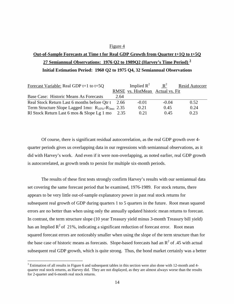
Figure 4
Out-of-Sample Forecasts at Time t for Real GDP Growth from Quarter t+1Q to t+5Q
27 Semiannual Observations: 1976 Q2 to 1989Q2 (Harvey’s Time Period) 3
Initial Estimation Period: 1960 Q2 to 1975 Q4, 32 Semiannual Observations
Forecast Variable: Real GDP t+1 to t+5Q Implied R2 R2 Resid Autocorr RMSE vs. HistMean Actual vs. Fit Base Case: Historic Means As Forecasts 2.64 Real Stock Return Last 6 months before Qtr t 2.66 -0.01 -0.04 0.52 Term Structure Slope Lagged 1mo: R10Yr-R3mo 2.35 0.21 0.45 0.24 Rl Stock Return Last 6 mos & Slope Lg 1 mo 2.35 0.21 0.45 0.23
Of course, there is significant residual autocorrelation, as the real GDP growth over 4-
quarter periods gives us overlapping data in our regressions with semiannual observations, as it
did with Harvey’s work. And even if it were non-overlapping, as noted earlier, real GDP growth
is autocorrelated, as growth tends to persist for multiple six-month periods.
The results of these first tests strongly confirm Harvey’s results with our semiannual data
set covering the same forecast period that he examined, 1976-1989. For stock returns, there
appears to be very little out-of-sample explanatory power in past real stock returns for
subsequent real growth of GDP during quarters 1 to 5 quarters in the future. Root mean squared
errors are no better than when using only the annually updated historic mean returns to forecast.
In contrast, the term structure slope (10 year Treasury yield minus 3-month Treasury bill yield)
has an Implied R2 of 21%, indicating a significant reduction of forecast error. Root mean
squared forecast errors are noticeably smaller when using the slope of the term structure than for
the base case of historic means as forecasts. Slope-based forecasts had an R2 of .45 with actual
subsequent real GDP growth, which is quite strong. Thus, the bond market certainly was a better
3 Estimation of all results in Figure 6 and subsequent tables in this section were also done with 12-month and 4-quarter real stock returns, as Harvey did. They are not displayed, as they are almost always worse than the results for 2-quarter and 6-month real stock returns.

15
forecaster than was the stock market for real GDP growth for quarters t+1Q to t+5Q during this
1976-1989 period. As Harvey noted, the term structure slope did an extremely fine job in
forecasting the large double dip recession in 1980 and 1981-82. Note that combining stocks with
the term structure slope did not improve the forecasting statistics from those of the slope alone.
Now let us examine the results when the ensuing 22 years of data are added. We had
three new recessions in this new data, 1991-1992, 2001-2002 and 2008-2009, with the last one
being dubbed the “Great Recession” or the “Financial Panic of 2008/2009.” For our new, full
51-year sample (1960-2011Q2), we again use the first 15 years of data (30 semiannual data
points from 1960 to 1974) as the initial estimation period for regressions and use those to
forecast the 2 semiannual observations for 1975. Then we update the regressions annually to
generate out of sample forecasts for each semiannual period (with data through 2011 Q2), where
our last observation is for Q4 2009, given the forward forecasts. Doing this, we have 35 years
of forecasts, whereas Harvey had only 13 years available for his forecasts.
The results of this extension using data to 2011Q2 are given in Figure 5. As can be seen,
neither the real stock return, nor the term structure slope model had more accurate forecasts than
simply using the historic means for real GDP growth 1 to 5 quarters out during the 1975 to 2009
period. The term structure slope is much less effective in forecasting over this full sample than it
was in the 1976-1989 period that Harvey examined. While the forecasts based on the stock
market’s recent return had no correlation with real GDP growth 1 to 5 quarters out, the forecasts
based on the term structure slope had an R2 of 0.26 with actual growth rates, so the bond market
based forecasts were more informative again in the full sample. However the bias in the term
structure model’s parameters caused its RMSE to be no better than that from historic means.

16
Figure 5
Out-of-Sample Forecasts at Time t for Real GDP Growth from Quarter t+1Q to t+5Q
71 Semiannual Observations: 1975 Q2 to 2010Q2 (Full Sample)
Forecast Variable: Implied R2 R2 Resid Autocorr RMSE vs. HistMean Actual vs. Fit Base Case: Historic Means As Forecasts 2.39 Real Stock Return Last 6 months to t 2.45 -0.05 0.00 0.59 Term Structure Slope Lg1m: R10Yr, R3mo Arith 2.43 -0.03 0.24 0.49 Slope (Lg1, Arith) & Last 6 months RlStocks 2.42 -0.02 0.25 0.43
The low ability of real stock returns to forecast real GDP growth is perplexing and
counterintuitive, as casual observation is that stock investors are obviously trying to forecast the
direction of the economy and appear to have some short-term ability to do so. To explore why
we are not picking up any ability in the above regressions, let us look at regressions with non-
overlapping data for all variables. What we have with the semiannual data set is the 2-quarter
growth rate in real GDP regressed on its lagged value (to pick up the autocorrelation) and on 2
lags of prior 2-quarter real stock returns. The results are in Figure 6 below, using the 1959-2011
Q2 period, for which we have monthly real consumption data, with a lag that causes the first data
point to be in 1960’s first half:

17
Figure 6
The very high t-statistics (-6.9 for unemployment changes, 4.5 for GDP, 5.4 for industrial
production) on the first lagged real stock return indicate a strong in-sample relationship for
forecasting ahead 2 quarters. However, note that the second lag has very weak t-statistics for
real GDP and industrial production (0.7 and 0.1), indicating that real stock returns show no in-
sample ability to explain more than two quarters ahead for those variables. There is a stronger
ability (t=2.7 and t= -1.9) of stocks to explain the employment growth rate and the change in the
unemployment rate for 3-4 quarters out, as those are slower moving than GDP and industrial
production. As the table shows, stock returns are less helpful in forecasting consumption
growth, as the t-statistic for its slope is only 1.7. Part of that is likely due to the fact that prior
consumption growth picks up the prior stock return, and the autorcorrelation of consumption
growth rates through time is significant.
Given that stocks appear to have in-sample forecasting ability for only about two quarters
forward, Harvey’s procedure of examining ability to forecast real GDP growth starting at t+1Q

18
and going to t+5Q may well miss quite a bit of the information of stock returns by not picking up
the first quarter forward’s real GDP growth, i.e., that from t = t+0 to t+1Q. For example, in the
middle of the fourth quarter, say November 15th, it is quite typical for economic forecasters to
estimate real growth from the fourth quarter of the current year to the fourth quarter of the
following year, rather than from the first quarter of next year to the first quarter of the following
year. Growth from the present 4th quarter to the first quarter of the next year is not yet known
and is a key part of the forecast. To capture this information, if it exists, we next re-run the
simulations with the dependent variable being the real growth of GDP from t= t+0 to t+4Q. As
we view the timing of that as centered at November 15th and May 15th, we will focus on the
results for percentage changes in real stock price averages for the 2nd and 4th quarters and not at
those in the last months of the second and fourth quarters, December and June, which would
have a significant look-ahead bias. The results of the simulations are in Figure 7:
Figure 7
Out-of-Sample Forecasts at Time t for Real GDP Growth from Quarter t+0Q to t+4Q
71 Semiannual Observations: 1975 Q2 to 2010Q2 (Full Sample)
Forecast Variable: Implied R2 R2 Resid Autocorr RMSE vs. HistMean Actual vs. Fit Base Case: Historic Means As Forecasts 2.32 Real Stock Return Last 2 Quarters 2.26 0.06 0.14 0.61 Term Structure Slope QAvg R10Yr, R3mo Arith 2.48 -0.14 0.26 0.57 Slope Arith QAvg & Last 2 Quarters Stocks 2.28 0.04 0.38 0.47 Starting at the current quarter t, the past 2-quarter real stock return (real stock price percentage
gain from quarter t-2 to quarter t) does have some ability to improve four quarter forward
forecasts going from t to t+4Q. The bond market’s term structure slope (average for quarter t)
again gives forecasts that are correlated with subsequent growth, but parameter estimation errors
during the simulation makes them poorer on RMSE versus using historic mean GDP growth.
The combination of stock and bond market signals also gives a reduced RMSE versus historic
mean forecasts, and with R2 values of 0.04 and 0.38, respectively.

19
The final experiment for stocks and bonds as forecasters of real GDP growth is to repeat
the above analysis for shorter forecasts – forecasts that go forward only two quarters from t =
t+0Q to t+2Q. Figure 8 has the results:
Figure 8
Out-of-Sample Forecasts at Time t for Annualizd Real GDP Growth Quarter t+0Q to t+2Q
72 Semiannual Observations: 1975 Q2 to 2010Q4 (Full Sample)
Forecast Variable: Implied R2 R2 Resid Autocorr RMSE vs. HistMean Actual vs. Fit Base Case: Historic Means As Forecasts 2.72 Real Stock Return Last 2 Quarters 2.45 0.19 0.23 0.31 Term Struct Slope Arith Lg1 QAvg R10Yr, R3mo 2.90 -0.14 0.17 0.32 Slope Arith Lg1, QAvg & Last 2 Qtrs Stocks 2.50 0.15 0.38 0.19 The result that past real stock returns do better (RMSE and Implied R2) than the bond
market’s term structure slope for the shorter forecasts is confirmed and even strengthened for the
closest forecast period, t to t+2Q. Adding the 10 year – 3 month term structure slope does not
improve short-term forecast accuracy beyond that for real stock returns alone. However, the
forecasts have a much higher correlation with subsequent growth again when both past stock
returns and the term structure slope are considered in the forecasts, as the R2 of the regression of
actual on forecasts jumps from 0.23 to 0.38.
Given the significant autocorrelation in real GDP growth, even when non-overlapping
data are used (and even more so with overlapping forecast periods), it is instructive to compare
forecasts based on autoregressive models with the term structure slope and past real stock returns
and the performance of simple, first-order autoregressive model for real GDP growth. Figure 9
shows that the simple autoregressive model for real GDP growth does well, with an implied R2
of 0.22 and a correlation of forecasts with actuals R2 of 0.19. Adding the lagged term structure
slope to prior GDP growth does not improve forecast accuracy. However, adding prior stock
returns does improve forecast accuracy and the R2 measures increase to 0.29 and 0.31.

20
Figure 9
Out-of-Sample Forecasts: Time t for Annualized Real GDP Growth Quarter t+0Q to t+2Q
Autoregressive Models. 72 Semiannual Observations: 1975 Q2 to 2010Q4 (Full Sample)
Forecast Variable: Implied R2 R2 Resid Autocorr RMSE vs. HistMean Actual vs. Fit Base Case: Historic Means As Forecasts 2.72 1st Order Autoregressive Model for Real GDP 2.40 0.22 0.19 0.09 Lg1GDP + Real Stock Return Last 2Q QAvg 2.28 0.29 0.31 0.16 Lg1GDP +Term Struct Slope Lg1 QAvg 2.62 0.07 0.26 0.18 Lg1 GDP, Lg1 Slope QAvg & Last 2Q Stocks 2.37 0.24 0.42 0.08 In summary for the results of tests for real GDP forecasts, both real stock returns and the
term structure slope stand as key variables in forecasting the growth rate of real GDP. Real
stock returns in the past 6 months or two quarters give the greatest reduction in RMSE in out of
sample forecasts for real GDP (12% reduction of forecast errors with an AR1 model increases to
a 17% reduction when the recent stock return is utilized), with almost all of the forecasting
ability concentrated in the two quarters following the forecast. The term structure slope is
correlated with subsequent real GDP growth, but the difficulties of errors in estimating the
constant term and slope of that relationship makes it less effective in reducing RMSE for real
GDP. Indeed, in many of the simulations, using the term structure slope increases forecast errors
over those using stock returns alone in this full sample period from 1975 to 2010.
Next, we examine 6-month-ahead in-sample forecast results for changes in the
unemployment rate, employment growth, industrial production and real consumption growth.
Note that the R2 values for reduction of forecast errors are very high (50%, 42% and 38%,
respectively) for 6-month percentage changes in the unemployment rate, total employment
growth and industrial production. Careful scrutiny of Figure 10 shows that the stock market’s
return is most effective in these out-of-sample forecasts. Adding the term structure slope to
forecasts based on stock returns improves the forecasts for each of these variables and improves
the correlation of forecasts with subsequent actuals, but not to the same degree that the stock
market return reduces forecast error.

21
As Hall (1981) and Lettau-Ludvigson (2001) found, Figure 10 also shows that the past
real stock market return and the term structure slope are not effective in forecasting real
consumption growth out of sample, as a simple AR1 model provides the lowest RMSE for real
consumption growth. The next section will model real consumption growth deviations from
stock market wealth effects and demonstrate that consumers also have useful information for
forecasting the movements in the growth of real GDP, industrial production, total jobs in the
economy and changes in the unemployment rate. The combination of information from the stock
market, the bond market, and consumers provides even better forecasting results than with just
stock and bond market data.

22
Figure 10
Out-of-Sample Forecasts with AR1 Models at Time t for 6-month Growth of Industrial
Production, Total Employment & Changes in the Unemployment Rate t+0 to t+6 months
73 Semiannual Observations: 1975 Q2 to 2011 Q2 (Full Sample)
Forecast Variable (Y): Change Unemployment Rate Implied R2 R2 Resid Autocorr (Note: 2 x 6-month change in U) RMSE vs. HistMean Actual vs. Fit Base Case: Historic Means As Forecasts 1.35 1st Order Autoregressive Model for Y Variable 1.19 0.22 0.19 0.12 Lg1Yvar + Real Stock Return Last 6mos 1.00 0.44 0.43 0.04 Lg1Yvar + Lg,Lg2 6m Real Stock Return 1.01 0.44 0.43 0.22 Lg1Yvar +Term Structure Slope Lg1m 1.17 0.25 0.28 0.18 Lg1 Yvar, Lg1m Slope & Last 6mos RlStocks 0.95 0.50 0.51 0.02
Forecast Variable (Y): %Growth Employment(Jobs) Implied R2 R2 Resid Autocorr Note: Growth % is annualized. RMSE vs. HistMean Actual vs. Fit Base Case: Historic Means As Forecasts 1.97 1st Order Autoregressive Model for Y Variable 1.66 0.29 0.27 0.04 Lg1Yvar + Real Stock Return Last 6mos 1.52 0.41 0.40 -0.07 Lg1Yvar + Lg1,Lg2 6m Real Stock Return 1.52 0.40 0.41 0.14 Lg1Yvar +Term Structure Slope Lg1m 1.64 0.30 0.35 0.12 Lg1 Yvar, Lg1m Slope & Last 6mos RlStocks 1.50 0.42 0.47 -0.02 Forecast Variable (Y): Industrial Production Implied R2 R2 Resid Autocorr RMSE vs. HistMean Actual vs. Fit Base Case: Historic Means As Forecasts 5.68 1st Order Autoregressive Model for Y Variable 5.18 0.17 0.13 0.10 Lg1Yvar + Real Stock Return Last 6mos 4.52 0.37 0.37 0.06 Lg1Yvar + Lg,Lg2 6m Real Stock Return 4.57 0.35 0.36 0.12 Lg1Yvar +Term Structure Slope Lg1m 5.28 0.14 0.27 0.20 Lg1 Yvar, Lg1m Slope & Last 6mos RlStocks 4.46 0.38 0.48 0.12 Forecast Variable (Y):Growth Real Tot Consumption Implied R2 R2 Resid Autocorr Note: Growth % is annualized. RMSE vs. HistMean Actual vs. Fit Base Case: Historic Means As Forecasts 2.25 1st Order Autoregressive Model for Y Variable 2.02 0.20 0.16 0.08 Lg1Yvar + Real Stock Return Last 2Q 2.10 0.12 0.12 0.17 Lg1Yvar + Lg,Lg2 2Q Real Stock Return 2.18 0.06 0.09 0.28 Lg1Yvar +Term Structure Slope Lg1QAvg 2.08 0.14 0.27 0.15 Lg1 Yvar, Lg1 SlopeQavg & Last 2Q RlStock 2.12 0.11 0.25 0.12

23
III. Real Consumption Spending As A Leading Indicator
This section shows that real consumption growth deviations from growth predicted by
wealth effects add significantly to stock returns and the term structure slope in forecasting
macroeconomic changes in unemployment, employment, real GDP, industrial production, real
personal income and real wage growth. This is true for real, aggregate consumption measured
with just nondurables and services, as well as with real total consumption, including durables.
Thus, it will be shown that real consumer spending growth is, indeed, a leading indicator. While
the strength of its forecasting increment is not as much as for the stock market’s real return, it is
similar to that of the term structure slope, and sometimes is of greater impact than the slope.
The combined regression results will give us a “Stocks, Bonds, Consumers Leading Indicator
(SBCLI),” which is further developed in the next section and in a companion applied paper.
Indeed, these three key variables, which are very well grounded in economic theory, have a
forecasting ability that is quite similar to (and often seems better than) that of the Conference
Board’s highly regarded Index of Leading Economic Indicators.
In the theory of intertemporal consumption and portfolio choice, Samuelson (1969),
Merton (1969, 1971, 1973), Fama (1970), Rubinstein (1974, 1976), Breeden-Litzenberger
(1978), Breeden (1979, 1984, 2004) and many others modeled optimal consumption choices as a
function of wealth, the state of investment, consumption and job opportunities, and time (age).
Breeden’s (1979) continuous-time model derivation of optimal consumption’s sensitivities to
opportunity set state variables in terms of derivatives of the indirect utility function for wealth
was the key to his collapsing Merton’s multi-beta intertemporal CAPM into the single-beta
consumption CAPM.
In Breeden (1984), it was shown that with power utility, optimal consumption is
increasing in investment opportunities (and normal hedging behavior is optimal) if and only if
relative risk aversion exceeds unity (logarithmic utility). If an individual were less risk averse
than with logarithmic utility, optimal consumption actually should decrease with better
investment opportunities (“reverse hedging” is optimal), so that more could be invested to take

24
advantage of the better investments. This leads to a higher multi-period mean consumption path,
but higher variance.
The extensive literature on the “equity premium puzzle” and other tests overwhelming
estimates that a typical investor’s risk aversion is much greater than that of logarithmic utility,
with estimates ranging from 2 to 50 for relative risk aversion. Thus, we believe that most
consumers exhibit normal intertemporal hedging behavior, in that better job or investment
opportunities are reflected in higher current consumption, as a higher level can be sustained with
better opportunities, holding current wealth constant. Breeden (1991) turned it around and said
that if consumption was high, relative to wealth, then it should be that consumers predict better
investment or job opportunities (e.g., quantities of jobs or wage levels). Thus, consumption
deviations from those predicted by wealth moves should be leading indicators of changes in job
or investment opportunities. His initial tests provided some significant results, which we expand
upon in this section. Lettau and Ludvigson’s (2001) results and Uhlig’s (2007) model are also
related to these fundamental optimal responses of consumers to the labor income opportunity set.
Lettau and Ludvigson’s important work find that when consumption is high relative to wealth,
subsequent investment returns are on average 2% higher annually than when the
consumption/wealth ratio is low.
A. Computing Consumption Deviations from Wealth Effects, C┴
As an overview of the relationship of real consumption growth to real stock returns, both
contemporaneous and for the prior 6-month period, let us first look at the results of the full
sample regressions, using the semiannual data from 1960 to 2011 Q2, a 51 year period with 103
nonoverlapping observations. Regressing real consumption growth separately for total
consumption (PCETot) and for nondurables and services consumption (PCE NDS) on both
contemporaneous real stock market returns and lagged returns, we find that the current 6-month
real stock return (t=5.2 and t=4.7) and the prior 6-month stock return (t=2.8 and t=2.2)
significantly affect current 6-month real consumption growth, as shown in Fig. 11:

25
Figure 11
In Figure 12, we use quarterly data for consumption and stock returns, instead of monthly data,
as some key macro variables (like GDP and corporate profits) are measured only quarterly. This
gives 2-quarter consumption deviations that have time aggregation properties that match up
properly with corporate profits and GDP. Careful comparison of Figure 12’s results with those
of Figure 11 shows that little is lost by using the 2-quarter change data, rather than the 6-month
consumption and stock return data.
Figure 12

26
The greater significance of the lagged effect of stock market wealth on total consumption than
for NDS consumption likely indicates that the effect of stock returns on consumption of durables
is a longer-term response than for nondurables and services.
The examination of consumer behavior as a leading indicator takes the residuals from
the above regressions of consumption on stock market returns, which we will call “consumption
deviations (c┴)” (from wealth effects), and tests to see if they are predictive of future periods’
jobs, real wages and investment opportunities. We look at future changes in the unemployment
rate, the total number of persons employed, and the growth rate of real wages and personal
income to measure consumption deviations’ abilities to predict changes in the labor market
opportunity set.
Of course, the coefficients in the full-sample regressions just examined in Figures 11 and
12 could not have known until 2011, when all of this data was available. To compute the
consumption deviations that individuals could more realistically have estimated at each point in
time, we again do simulations based on regressions with prior data. The annually updated
regressions that were computed for real total consumption growth on contemporaneous and prior
stock returns are in Appendix 1A, while those for the growth of real nondurables and services
consumption are in Appendix 1B. Our time series of consumption growth deviations variables
(for total and NDS consumption, respectively) are their actual real annualized growth rates, less
the growth that would have been expected given the stock market’s performance and given the
OLS relationship estimated with prior data, updated annually.
For the USA for years 1960-1974, the consumption deviations variables are from in-
sample regression residuals using data covering that period, whereas the 1975-2011 Q2
consumption deviations are all out-of-sample forecasts from the expanding regressions. The
consumption deviations data for the in-sample 1960-1974 time period are only used subsequently
to derive the first estimates of the relationships of other variables (like real GDP growth) to
consumption deviations, in addition to the stock market return and the term structure slope. All
forecast errors that will then be examined for GDP on stocks, bonds and consumption deviations
are for out-of sample forecasts (1975-2011).

27
Before looking at the results for consumption deviations’ relationships to the job and
investment opportunity sets, let us first look at the behavior of this new third factor as compared
with the two prior major factors – stock returns and the term structure slope. For stock returns,
we know that by construction of the deviations, this new factor will be independent of past stock
returns, as ordinary least squares regressions always yield that for their errors. Figure 13 plots
the 10-year – 3-month term structure slope versus the consumption deviations for real total
consumption and finds that they are quite different variables, sometimes moving together,
sometimes in opposite ways. The R2 in a regression of one on the other is -0.01, so they are also
orthogonal. Given this, multi-collinearity should not be a significant problem for our subsequent
regression estimates, as each variable is quite different.
Figure 13
To see the univariate relationship of consumption deviations with unemployment rate
changes, Figure 14 plots the time series of both series, with the consumption residuals being

28
from the past two 6-month periods, as unemployment changes are forecasted by consumption
deviations up to 12 months in advance. When consumption deviations are positive, the
unemployment rate subsequently falls. When consumption deviations are negative, the
unemployment rate subsequently increases, as consumers have knowledge about the job market
when they choose what to spend.
Figure 14
B. In-Sample Stepwise Regressions: Consumption Deviations Combined with Real
Stock Returns and the Slope of the Term Structure
Since there is little correlation among the three key factors – real stock returns, the slope
of the term structure, and real consumption deviations from wealth effects -- when lagged
consumption deviations are added in regressions explaining 6-month unemployment rate

29
changes, they come in with solid relationships and a multivariate t-statistic of t = -2.8 for total
real consumption and t = -3.2 for real nondurables and services (NDS) consumption.
Figure 18 shows the regression results for macroeconomic variables regressed upon their
prior values and on lagged stock returns, the lagged slope of the term structure, and real total
consumption growth deviations from wealth effects over the prior 12 months. Results for
regressions with nondurables and services consumption are very similar and are omitted. Note
that the 6-month real wage growth series has a large blip in 1993 that changes positive
autocorrelation to negative autocorrelation in the regression simulations. To see more normal
results, results for the 2-quarter changes in real wage growth are also shown. The same is done
for personal income less transfers.
Figure 18

30
Figure 18 demonstrates that consumption deviations have strong statistical significance in
explaining fluctuations in the unemployment rate, in total employment, in explaining real GDP
growth, industrial production growth, personal income growth and wage growth. This is as
theory predicts, as we expect that individuals are considering their job market and income
opportunities carefully as they choose their optimal consumption spending. Higher consumption
deviations from wealth indicate knowledge of a good job market and wage and income
prospects. When consumption is low relative to wealth, consumers likely are reflecting their
knowledge of a poor job market and likely poor future real income growth.
To see the incremental effects of each of the variables, starting with the stock market and
then the slope of the term structure, and now with consumption deviations from wealth, Figure
19 gives corrected R-squared values from stepwise regressions for both the total consumption
deviations and the NDS consumption deviations. In addition, results are shown for the
Conference Board’s Index of Leading Economic Indicators.
Figure 19

31
As we can see, consumption deviations appear to be an effective third key variable in leading
important macroeconomic fluctuations, as they add significantly to in-sample explanatory power
from stock and bond markets for employment, unemployment, real GDP growth, and for real
personal income and wage growth. In sample, our three-factor stocks/bonds/consumers model,
SBCLI, fits the data better than the index of leading economic indicators, LEI, for employment
growth, for unemployment rate changes and for real wage and personal income growth.
For real GDP growth and industrial production growth, explanatory power in sample is almost
identical between the LEI and the SBCLI model. We will now see if these in-sample results hold
up in the simulation of out-of-sample forecasts.
C. Out-of-Sample Forecast Performance
As Figure 19 shows, the in-sample fits of our three key variables, reflecting knowledge in
the stock market, the bond market and of consumers, are quite similar to those of the entire set of
10-12 indicators in the LEI. This is certainly promising, as these three variables are quite
understandable and intuitive, in contrast to the much more complex and less intuitive Index of
Leading Economic Indicators (LEI). While each variable in the LEI makes sense as an economic
indicator, one knows that these were largely chosen from hundreds of variables examined for
their statistical forecasting performance, rather than from a sense of top economic priority. In
contrast, the information of stock investors, bond investors and the aggregate of 300 million
consumers in the USA would likely be the top three sources of broad information pools that
many economists would identify.
In this next segment, we show the results of out-of-sample simulations like those of
Section II for stocks and bonds, but now examining whether consumption deviations can further
reduce forecast errors, given the challenges in estimating parameters over time, without looking
ahead to data yet to come. In Section II, there were several instances when stock market and
term structure variables had strong t-statistics (often 3 or 4) in regression fits, but actually had
worse forecasting performance (RMSEs) out of sample than a naïve model of simply estimating
the historic mean for the Y-variable. This poor performance out of sample presumably is due to
difficulties of estimating the parameters of the relationships in advance, without knowledge of

32
the subsequent full sample of data. Constant and slope coefficients for the variables are all
parameters to be estimated. Difficulties in estimating these coefficients can substantially reduce
or even eliminate the forecast improvements from a seemingly strong (ex post) variable.
A summary of the results of the out-of-sample forecast simulations is in Figure 20.
Appendix 2 contains the annual estimated coefficients for the regression of the change in the
unemployment rate on 2 lags of real stock returns (covering the prior year), the term structure
slope at the beginning of the forecast period, and 2 lags averaged of the NDS consumption
deviation (also covering the prior year’s c┴). As in Section II, the initial estimation period was
1961 to 1974 (losing 1960 data due to the 2 lags from the consumption deviations, which were
estimated in part from prior stock returns in 1959). A benchmark naïve model that used trailing
mean values for the Y variable was used to create a base case root mean squared error. The new
model was then fit and its RMSE computed and then an “implied R2” was computed that reflects
the percentage reduction in RMSE squared. These were done in a stepwise manner to give the
results in Figure 20.
Figure 20

33
The simulations show that the in-sample model comparisons very broadly held up.
Consumption deviations improved out-of-sample forecast performance for all macro variables
except for Industrial Production, where its in-sample statistics were also weak (t=1.6). For
employment, unemployment, and real GDP, consumption deviations were effective leading
indicators in this simulation, adding to the forecasting power of the stock and bond markets.
For all of these major macro variables, the “Stocks, Bonds, Consumers leading index” (SBCLI)
has out of sample forecast performance that is better than for the venerable Index of Leading
Economic Indicators. These excellent results certainly deserve further scrutiny.
The next section presents similar analysis of stocks, bonds and consumers as leading
indicators for the three global mega-economies -- advanced economies in the Americas, in
Europe and in AustralAsia.
IV. Global Stocks, Bonds, Consumers as Leading Indciators
In this section, we examine data for large, advanced economies in the Americas, Europe
and AustralAsia, drawn primarily from the Organization for Economic Cooperation and
Development (OECD) website, as well as from the International Monetary Fund’s International
Financial Statistics (IFS) database. Global Insight and DataStream were also helpful in finding
some of the data. Data for 13 advanced economies are represented in three composites for these
mega-economies: (1, 2) USA and Canada are the trillion dollar advanced economies in the
Americas; (3-7) Germany, France, United Kingdom, Italy and Spain are the 5 trillion dollar
advanced economies in Europe; and (8-13), Japan, Australia (1970 on) and South Korea, Hong
Kong, Singapore and Taiwan (all 1990 onward) make up the AustralAsia composite. Each of
these economies has $1 trillion of GDP in US dollars in 2012, with Hong Kong, Singapore and
Taiwan combined to get one trillion dollar economy. The GDP weights in the three global
mega-economy composites are given in Figure 21:
Figure 21

34
3 Global Mega-Economy Composites: Percentage Weights Trillion Dollar Economies (TDEs) with GDP/Capita>$US 10,000
1970 1990 2010
Advanced America TDEs 100.0% 100.0% 100.0%
United States 90.3 89.8 90.0
Canada 9.7 10.2 10.0
Advanced Europe TDEs 100.0% 100.0% 100.0%
United Kingdom 47.3 20.8 22.4
Germany 18.5 27.2 28.2
France 14.8 22.1 21.1
Italy 11.6 19.9 16.9
Spain 7.9 9.9 11.3
Advanced AustralAsia TDEs 100.0% 100.0% 100.0%
Japan 90.4 77.7 63.6
Australia (added 1970) 9.6 8.2 14.4
South Korea (added 1990) 0.0 7.0 11.8
Hong Kong, Singapore, Taiwan (1990) 0.0 7.1 10.2
For each of the three mega-economies, real GDP growth, real consumption growth,
industrial production growth, inflation, real stock returns, unemployment rate changes, and total
employment growth were estimated using weighted averages of individual country data for those
variables, as that data became available. Different countries had data starting at different dates.
In the Americas, complete data was available for both the USA and Canada for the entire sample,
which we started in 1960 for this global analysis with quarterly data. In Europe, between the
U.K. and Germany (West Germany before reunification) composites for data on all variables
examined in this section could be formed from 1962 onward. France and Italy also had data on
certain variables available in the OECD or IFS data sets in the 1960s and were used in the
composites when data were available. Spain generally had data starting in the 1970s. In
AustralAsia, Japan had complete data from 1961 onward. Australia was added to the composite
starting in 1970, and the four “Asian Tigers,” (South Korea, Hong Kong, Singapore and Taiwan)
were added in 1990, when their GDP per capita was approximately $10,000 US.

35
Over this 50 year period analyzed, growth rates changed quite a lot, as all economies
developed and matured and growth slowed. Beginning with data in 1961, a 5-year average
growth rate of real GDP was calculated for each mega-economy. This was expanded to a 20-
year moving window as time passed and additional data arrived. Figure 22 below shows the
growth trends for each of the three areas. These will be used for our nonlinear time trend
variable in almost all regressions and simulations. In the statistical results, this gives better
explanatory power than linear time trends, as when economies mature, their growth rates have
tended to flatten out at 2% to 3% real growth rates.
Figure 22
The real consumption deviations from stock market wealth variable, c┴ or “c-perp”, was
estimated as the residuals in the regressions presented in Figure 23. Of course, lagged values of
this are used for the consumption variable in the SBCLI leading indicator.
0
2
4
6
8
10
12
1966
1219
6806
1969
1219
7106
1972
1219
7406
1975
1219
7706
1978
1219
8006
1981
1219
8306
1984
1219
8606
1987
1219
8906
1990
1219
9206
1993
1219
9506
1996
1219
9806
1999
1220
0106
2002
1220
0406
2005
1220
0706
2008
1220
1006
Long Term Trends in Real GDP Growth. Last 5 Years Growing to Last 20 Years Window
AdvAustralAsia Historic Growth 5-20 yrs Aamericas Historic Growth 5-20 Years
Adv Europe Historic Growth 5-20 Years
AAsia
Adv Americas
Adv Europe

36
Figure 23
3 Mega-Economies: Removing the Wealth Effect from Consumption: Real Consumption Growth Predicted by Stock Returns
2 Quarter Changes (Q2-Q4-Q2). 50 Years: 1961 – Q2/2011
Dependent VarReal TotalConsumptionGrowth (2Q%, Annlzd)
RealStockReturn2Q%
Current
Real Stock Return 2Q% Lag1
RealStockReturn2Q% Lag 2
20 YrHistoricTrend
GrowthRl GDP Const
CorrRSQ
Advancd Americas 0.093 0.058 0.041 0.87 -0.29 0.391961Q2-2011Q2 t=5.4 t=3.3 t=2.4 t=4.6 t= -0.4 N=101
Advanced Europe 0.035 0.032 0.017 1.15 -1.15 0.411962Q2-2011Q2 t=3.0 t=2.7 t=1.4 t=7.9 t= -2.2 N=97
Advanced AusAsia 0.051 0.025 0.022 0.83 -0.93 0.461961Q2-2010Q4 t=2.6 t=1.3 t=1.1 t=8.5 t= -1.5 N=100
From Figure 23, one can see that in each of the areas, real consumption growth over 2-
quarter periods (Q2-Q4-Q2) was significantly related contemporaneously to real stock market
returns in each mega-economy over the past 50 years, with t-statistics ranging for 2.6 for
AustralAsia to 3.0 for Europe and 5.4 for the USA. A 10% real stock market return was related
to an 0.90% increase in annualized real consumption growth over the same 2-quarter period in
the USA, but only an 0.35% consumption increase in Europe and an 0.51% increase in
AustralAsia. Lagged effects were also present for up to a year in advance, with 2 2-quarter lags
having significance in the USA regression. Note that the time trend variable was quite
significant (with coefficients near 1.0), as the long-term time trend in real consumption growth
mimicked the long-term time trend in real GDP.
Next, the in-sample regressions were conducted for the major macroeconomic variables
on the real GDP historic trend growth, lagged values of real stock returns, the slope of the term
structure (OECD “long rate” minus OECD “short rate”), and the real consumption deviations
from the regression residuals of Figure 23. These macro variables were also related to the
OECD’s indexes for Leading Economic Indicators for each mega-economy (computed as a

37
weighted average of the individual countries’ trend restored growth rates). The regression
results for the Americas, Europe and AustralAsia are in Figure 24a-c:
Figure 24a
Figure 24b

38
Figure 24c
Perusing Figures 24a-e, the in-sample results, one can see that the signals from the stock
market, the bond market and from consumers are all normally quite helpful in explaining in-
sample variation in real GDP growth, in industrial production growth, changes in the
unemployment rate and the growth rate of total employment. Real consumption deviations
appear to be helpful in explaining subsequent macro variable moves in each of the mega-
economies and for each of the four macro variables.
The corrected R-squareds from regressions done in a stepwise manner are shown in
Figures 24d and 24e:
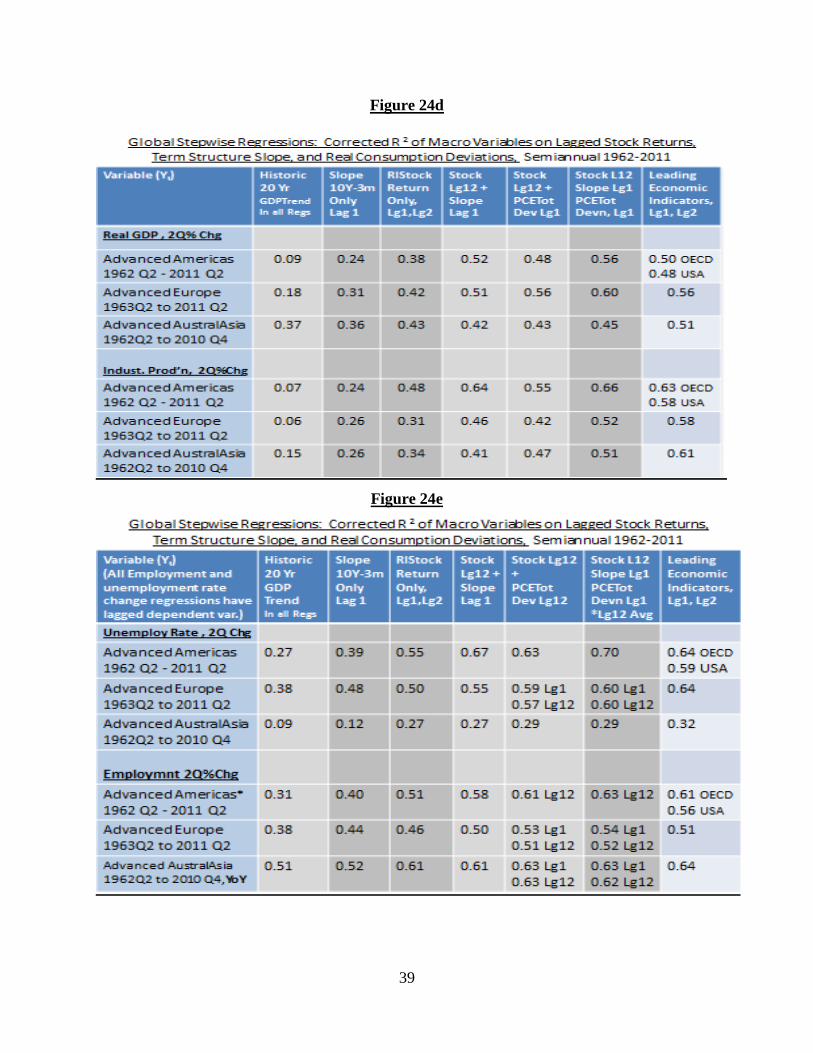
39
Figure 24d
Figure 24e

40
More important are the out-of-sample forecast results in Figures 25a and 25b, which were
computed in the same manner as in prior sections of the paper. Fifteen years of data are lost for
training the regressions for subsequent simulations, and the window for estimating coefficients is
expanded as time passes. Thus, the simulation period covers the 1977 to 2011 Q2 period for the
Americas and for Europe. For AustralAsia, the impact of the earthquake, tsunami and nuclear
meltdown in Japan in early 2011 caused abnormally large moves in several variables, so the data
set for Asia is stopped at Q4 2010.
The results shown are generally similar to those found for the USA in earlier sections. In
most of the simulations, the real stock market return, the slope of the term structure and the real
consumption deviation each add predictive power about real GDP growth, industrial production
growth, unemployment rate changes and total employment growth. There are a few anomalies,
such as the term structure slope not being helpful in explaining real GDP growth in AustralAsia
and the poor performance of the stock market in explaining growth, employment and
unemployment in Europe.
As the results for stock market information and slope of the term structure are likely
anticipated from Harvey’s and others’ results, the more significant new results are probably those
for the real consumption deviations variable, c-perp. It is helpful in forecasting each of the
variables in each mega-economy, perhaps with the exception that it doesn’t add explanatory
power for industrial production growth in the Americas, once the stock return and term structure
slope are considered.

41
Figure 25a
Figure 25b

42
From Figures 25a and 25b, one can see that the three Stocks, Bonds, and Consumers key
variables give out-of-sample forecast errors that are similar to those of the OECD’s and USA’s
indexes of leading economic indicators. It is notable that the leading indicators for Europe
appear especially difficult to beat in performance. This is worthy of further study into what they
are picking up that is not being picked up by our 3 key variables. It is also notable that the
European LEI and the OECD LEI for the USA both do better on employment related variables,
and less well on real GDP growth. (Perhaps there is a different objective in their construction?)
However, aside from that, it appears that the simple 3 key variables SBCLI model does as well
on average as the LEI computations, which usually use 7 to 12 variables in their construction.
Note that one of the disappointments in both the in-sample and out-of-sample forecasts
for the full sample period has been the performance of the bond market indicator used – the slope
of the term structure of interest rates (10-year yield less 3-month yield on Treasury securities).
Section V considers the term structure of inflation and the related term structure of real interest
rates using data for the USA. Taking this into account, the results show that the model can be
further enhanced.
V. Term Structure of Inflation and the Slope of the Real Term Structure.
In a multi-good model with Cobb-Douglas preferences for goods and with possible
inflation, Breeden (1986, eqs. 46 and 47) derived the returns on nominal and real riskless bonds
in terms the term structure of real growth and volatility, and the term structure of inflation and
the consumption beta for inflation, (which determines the risk premium on the nominally riskless
asset). As we have not explicitly considered inflation in the results so far, the theory described
in prior sections should be assumed to be for real growth parameters.
A significant potential problem with this approach can be illustrated. In December 2010,
the 10-year nominal interest rate was approximately 3.20%, while the 3-month Treasury bill rate
was approximately 0.10%, giving a term structure slope of 310 basis points. However, the
December 2010 survey by the Philadelphia Federal Reserve Bank (updating the long time series

43
begun by Joseph Livingston since 1946) shows that economists were forecasting inflation in
December 2010 at 1.3% for the next 6 months and 2.5% for the next 10 years. Thus, the term
structure of inflation had an upward slope of 120 basis points between 6 months and 10 years. In
real terms, the 3-month Treasury bill had a yield of approximately -1.20% and the 10-year
Treasury note a real yield of 0.70%. The slope of the term structure in real terms was only 190
basis points, much less than the 310 basis points indicated by the nominal term structure.
The Livingston/Philly Fed survey has been conducted semiannually in June and
December each year since 1946, so it fits well with the semiannual timing of our research. To
compute real short-term Treasury rates, we use the shortest term inflation forecast (6 months).
For long-term real rate estimates, we use the longest-term inflation forecast in the
Livingston/Philly Fed survey (12 months until 1974, 2 forecasts for 1974-1990 and 10 year
forecasts since 1990). With this data, we compute estimates for the slope of the real term
structure of interest rates and compare them to the slope for the nominal term structure. A time
series graph of these series is in Figure 26:
Figure 26

44
As can be seen, the real and nominal slopes are highly correlated in their movements (ρ = 0.92),
so the results should not change substantially by looking at the slope of the real term structure.
However, the timing of the largest differences is generally during the significant recessions and
in 1981/1982 and in 2008/2009 and their aftermaths. Thus, these differences could be important
at critical turning points in the economy.
Using this forward-looking estimated slope of the real term structure, instead of the slope
of the nominal term structure, all of the analyses were re-done. A comparison of the results
using the real term structure slope vs. the slope of the nominal term structure is in Figure 27.
Figure 27
Careful study of Figure 27’s results shows that replacing the slope of the nominal term
structure with that from the estimated real term structure does improve the results in each of
these macro variables, significantly so for industrial production, real personal income and real

45
wages. Thus, the slope of the term structure of inflation does matter for the interpretation of the
slope of the nominal term structure. In each of these cases, the margin of performance
improvement vis a vis the index of leading indicators is increased. These must be viewed as
preliminary results, as there are well-known challenges in using data on inflation forecasts.
V. Conclusion
We have shown that consumer behavior is a leading indicator. Real consumption
deviations from real stock market wealth effects add predictive value to that reflected in stock
price moves and the slope of the term structure of interest rates. In addition to considering stock
market wealth in their consumption expenditures, consumers apparently use knowledge of future
job market growth and wage growth in choosing their optimal consumption expenditures, as they
should.
It was also shown that these three well-founded economic variables, reflecting
information from the stock market, the bond market and consumers, gives explanatory power
that is similar or apparently slightly better than that of the Conference Board’s and the OECD’s
well-respected indexes of 7-12 Leading Economic Indicators. Thus, this simple model can help
decision makers deal with economic uncertainty better by helping them understand and compute
the key fundamentals giving clues to future growth.

46
References
Bansal, Ravi and Amir Yaron, 2004, Risks for the Long Run: A Potential Resolution of Asset Pricing Puzzles, Journal of Finance, August, pp. 1481-1509. Breeden, Douglas T., 1979, An Intertemporal Asset Pricing Model with Stochastic Consumption and Investment Opportunities, Journal of Financial Economics 7, Septebmer, pp. 265-296. Breeden, Douglas T., 1984, Futures Markets and Commodity Options: Hedging and Optimality in Incomplete Markets, Journal of Economic Theory 32, pp. 275-300. Breeden, Douglas T., 1986, Consumption, Production, Inflation, and Interest Rates: A Synthesis, Journal of Financial Economics 16, May, pp. 3-39. Breeden, Douglas T., Michael R. Gibbons and Robert H. Litzenberger, 1989, Empirical Tests of the Consumption-Oriented CAPM, Journal of Finance, June, pp. 231-262. Breeden, Douglas T., 2004, Optimal Dynamic Trading Strategies, Economic Notes, Vol. 33, No. 1, pp. 55-81. Campbell, John Y. and John H. Cochrane, 1999, By Force of Habit: A Consumption-Based Explanation of Aggregate Stock Market Behavior, Journal of Political Economy, April, 205-251. Cochrane, John H. and Monika Piazzezi, 2008, Decomposing the Yield Curve, University of Chicago working paper, March. Constantinides, George M., 1990, Habit Formation: A Resolution of the Equity Premium Puzzle, Journal of Political Economy 98, June, pp. 519-543. Fama, Eugene F., 1981, Stock Returns, Real Activity, Inflation and Money, American Economic Review, September, pp. 545-565. Fama, Eugene F. and Kenneth R. French, 1989, Business Conditions and Expected Returns on Stocks and Bonds, Journal of Financial Economics, November, pp. 23-49. Gomes, Joao F., Leonid Kogan and Motohiro Yogo, 2009, “Durability of Output and Expected Stock Returns,” Journal of Political Economy 17, no. 5, pp. 941-986. Grauer, Frederick L. A. and Robert H. Litzenberger, 1979, The Pricing of Nominal Bonds and Commodity Futures Contracts Under Uncertainty, Journal of Finance, March, pp. 69-84. Hall, Robert, 1978, Stochastic Implications of the Life Cycle-Permanent Income Hypothesis: Theory and Evidence, Journal of Political Economy, December pp. 971-987. Hansen, Lars P. and Kenneth J. Singleton, 1983, Stochastic Consumption, Risk Aversion, and the Temporal Behavior of Asset Returns, Journal of Political Economy 91, 249-265.

47
Harvey, Campbell R., 1988, The Real Term Structure and Consumption Growth, Journal of Financial Economics, December. Harvey, Campbell R., 1989, Forecasts of Economic Growth from Bond and Stock Markets, Financial Analysts Journal, September-October. Harvey, Campbell R., 1991, The Term Structure and World Economic Growth, Journal of Fixed Income, June. Hatzius, Jan, Peter Hooper, Frederic Mishkin, Kermit L. Schoenholtz and Mark W. Watson, Financial Conditions Indexes: A Fresh Look after the Financial Crisis, NBER, February 2010. Jagannathan, Ravi and Zhenyu Wang, 1996, The Conditional CAPM and the Cross-Section of Expected Returns, Journal of Finance 51, March, pp. 3-53. Jagannathan, Ravi and Yong Wang, 2007, Lazy Investors, Discretionary Consumption, and the Cross-Section of Stock Returns, Journal of Finance, August, pp. 1623-1661. Lettau, Martin and Sydney Ludvigson, 2001a, Consumption, Aggregate Wealth and Expected Stock Returns, Journal of Finance, June, pp. 815-849. Lettau, Martin and Sydney Ludvigson, 2001b, Resurrecting the (C)CAPM, Journal of Political Economy, December, pp. 1238-1287. Lucas, Robert E., 1978, Asset Prices In An Exchange Economy, Econometrica 46, 1429-1445. Mehra, Rajnish and Edward C. Prescott, 1985, The Equity Premium: A Puzzle, Journal of Monetary Economics 15, March, pp. 145-161. Merton, Robert C., 1971, Optimum Consumption and Portfolio Rules In a Continuous-time Model, Journal of Economic Theory, 373-413. Merton, Robert C., 1973, An Intertemporal Capital Asset Pricing Model, Econometrica, 41, 867-887. Parker, Jonathan A. and Christian Julliard, 2005, Consumption Risk and the Cross Section of Expected Returns, Journal of Political Economy, February, pp. 185-222. Rubinstein, Mark, 1976a, The Valuation of Uncertain Income Streams and the Pricing of Options, Bell Journal of Economics and Management Science 7, 407-425. Samuelson, Paul A., 1969, Lifetime Portfolio Selection By Dynamic Stochastic Programming, Review of Economics and Statistics, 239-246. Shiller, Robert J., 1982, Consumption, Asset Markets and Macroeconomic Fluctuations, Carnegie-Rochester Conference Series on Public Policy 17, Autumn, pp. 203-238.

48
Appendix 1A Simulation results from regressions with prior nonoverlapping data. Coefficients estimated with annual regressions were: Real Total Consumption Growth, 6 months, Annualized (CTot6m) is regressed upon: Constant t RlStok6m t Lg1Stk6m t CRSQ Observations Used 3.913 9.63 0.133 3.68 0.081 1.98 0.384 3 32 30 196006 197412 3.948 10.37 0.142 4.64 0.072 2.32 0.418 3 34 32 196006 197512 3.978 11.06 0.142 4.84 0.074 2.53 0.426 3 36 34 196006 197612 4.034 11.43 0.138 4.73 0.068 2.32 0.398 3 38 36 196006 197712 4.072 12.04 0.139 4.82 0.065 2.26 0.391 3 40 38 196006 197812 3.924 11.60 0.138 4.68 0.068 2.30 0.367 3 42 40 196006 197912 3.719 9.71 0.137 4.05 0.066 1.94 0.284 3 44 42 196006 198012 3.585 9.50 0.144 4.27 0.064 1.90 0.295 3 46 44 196006 198112 3.594 9.97 0.146 4.73 0.064 1.96 0.326 3 48 46 196006 198212 3.622 10.34 0.142 4.79 0.065 2.19 0.338 3 50 48 196006 198312 3.670 10.85 0.140 4.79 0.064 2.18 0.329 3 52 50 196006 198412 3.646 11.12 0.137 4.85 0.063 2.22 0.330 3 54 52 196006 198512 3.624 10.97 0.127 4.50 0.064 2.26 0.296 3 56 54 196006 198612 3.560 10.66 0.112 4.07 0.066 2.31 0.249 3 58 56 196006 198712 3.582 11.11 0.113 4.18 0.062 2.29 0.247 3 60 58 196006 198812 3.506 10.90 0.106 3.93 0.060 2.22 0.220 3 62 60 196006 198912 3.394 10.59 0.112 4.13 0.060 2.19 0.229 3 64 62 196006 199012 3.309 10.41 0.108 4.00 0.059 2.16 0.210 3 66 64 196006 199112 3.336 10.79 0.109 4.09 0.059 2.21 0.213 3 68 66 196006 199212 3.319 11.02 0.109 4.14 0.058 2.21 0.212 3 70 68 196006 199312 3.332 11.41 0.109 4.19 0.058 2.25 0.212 3 72 70 196006 199412 3.288 11.35 0.101 4.01 0.054 2.10 0.192 3 74 72 196006 199512 3.256 11.41 0.099 3.96 0.050 2.01 0.184 3 76 74 196006 199612 3.245 11.48 0.095 3.91 0.050 2.03 0.180 3 78 76 196006 199712 3.259 11.72 0.097 4.06 0.052 2.16 0.192 3 80 78 196006 199812 3.279 11.97 0.098 4.16 0.053 2.26 0.199 3 82 80 196006 199912 3.301 12.35 0.096 4.15 0.053 2.26 0.195 3 84 82 196006 200012 3.303 12.77 0.096 4.24 0.053 2.32 0.202 3 86 84 196006 200112 3.338 13.35 0.093 4.24 0.050 2.26 0.201 3 88 86 196006 200212 3.319 13.54 0.092 4.25 0.051 2.33 0.199 3 90 88 196006 200312 3.313 13.70 0.092 4.27 0.050 2.30 0.197 3 92 90 196006 200412 3.296 13.88 0.092 4.30 0.050 2.34 0.196 3 94 92 196006 200512 3.283 14.11 0.092 4.35 0.050 2.38 0.196 3 96 94 196006 200612 3.241 14.00 0.092 4.35 0.047 2.22 0.188 3 98 96 196006 200712 3.120 13.51 0.109 5.37 0.054 2.51 0.263 3 100 98 196006 200812 3.058 13.33 0.103 5.13 0.061 2.97 0.259 3 102 100 196006 200912 3.036 13.42 0.103 5.17 0.059 2.96 0.255 3 104 102 196006 201012 Constant t RlStok6m t Lg1Stk6mRl t CRSQ Observations Used

49
Out of Sample Forecast Errors and Implied R2 By Decade: BegDec EndDec Nobs HistMean ModelRMSE ImpRsq 1970 1979 10 2.277 1.965 0.256 1980 1989 20 2.971 3.007 -0.025 1990 1999 20 1.950 1.918 0.032 2000 2009 20 2.710 2.029 0.439 2010 2019 3 1.492 2.100 -0.981 Entire Estimation Period: Root mean squared forecast error = 2.308 Entire Estimation Period: RMSE using historic mean as forecast = 2.505 Entire Estimation Period: Implied R-Squared of Forecast = 0.151 Properties of Simulation fits and errors for observations: 33 to 105 ( 197506 to 201106 ) Dependent variable = Real Total Consumption Growth from t = t+0 months to t= t+6 months VARIABLE COEFFICIENT STD ERROR T-STAT(OLS) Constant -0.3375 0.7543 -0.45 Fitted 0.8607 0.1791 4.80 RSQ = 0.245 Durbin Watson = 1.56 CRSQ = 0.235 Autocorrel = 0.198 STD ERR = 2.1494 STD DEV (Y) = 2.457 Observs = 197506 to 201106 Nobs = 73 Deg of freedom = 71

50
Appendix 1B Simulation results from regressions with prior nonoverlapping data. Coefficients estimated with annual regressions were: Real Nondurables and Services Consumption Growth, 6 months, (Ann.) is regressed upon: Constant t RlStok6m t Lg1Stk6mRl t CRSQ Observations Used 3.801 13.25 0.080 3.13 0.038 1.32 0.275 3 32 30 196006 197412 3.770 13.98 0.081 3.74 0.030 1.36 0.290 3 34 32 196006 197512 3.798 14.83 0.081 3.87 0.033 1.56 0.296 3 36 34 196006 197612 3.797 14.96 0.081 3.84 0.030 1.40 0.278 3 38 36 196006 197712 3.840 15.68 0.081 3.88 0.027 1.28 0.268 3 40 38 196006 197812 3.752 15.56 0.080 3.81 0.028 1.31 0.252 3 42 40 196006 197912 3.635 13.96 0.080 3.47 0.027 1.14 0.204 3 44 42 196006 198012 3.517 13.42 0.086 3.68 0.025 1.06 0.216 3 46 44 196006 198112 3.485 13.83 0.089 4.10 0.028 1.23 0.252 3 48 46 196006 198212 3.502 14.35 0.086 4.17 0.029 1.40 0.259 3 50 48 196006 198312 3.517 15.03 0.086 4.26 0.029 1.41 0.259 3 52 50 196006 198412 3.516 15.57 0.085 4.40 0.029 1.48 0.268 3 54 52 196006 198512 3.462 15.18 0.077 3.96 0.025 1.27 0.219 3 56 54 196006 198612 3.448 15.46 0.071 3.86 0.026 1.39 0.202 3 58 56 196006 198712 3.462 16.09 0.072 3.97 0.025 1.36 0.203 3 60 58 196006 198812 3.429 16.02 0.068 3.78 0.025 1.40 0.183 3 62 60 196006 198912 3.342 15.51 0.073 3.99 0.025 1.36 0.195 3 64 62 196006 199012 3.275 15.20 0.070 3.80 0.024 1.32 0.173 3 66 64 196006 199112 3.292 15.70 0.070 3.88 0.025 1.36 0.176 3 68 66 196006 199212 3.268 15.95 0.070 3.92 0.024 1.34 0.173 3 70 68 196006 199312 3.262 16.39 0.070 3.98 0.025 1.39 0.175 3 72 70 196006 199412 3.228 16.28 0.065 3.74 0.020 1.17 0.150 3 74 72 196006 199512 3.205 16.40 0.063 3.68 0.018 1.06 0.142 3 76 74 196006 199612 3.194 16.43 0.060 3.56 0.017 1.03 0.131 3 78 76 196006 199712 3.197 16.72 0.061 3.70 0.017 1.06 0.139 3 80 78 196006 199812 3.221 16.92 0.062 3.79 0.019 1.19 0.145 3 82 80 196006 199912 3.240 17.44 0.061 3.77 0.019 1.19 0.141 3 84 82 196006 200012 3.199 17.63 0.063 3.97 0.022 1.40 0.157 3 86 84 196006 200112 3.186 18.19 0.064 4.17 0.023 1.49 0.173 3 88 86 196006 200212 3.160 18.32 0.063 4.11 0.024 1.57 0.167 3 90 88 196006 200312 3.151 18.57 0.063 4.14 0.023 1.54 0.166 3 92 90 196006 200412 3.140 18.89 0.063 4.18 0.024 1.57 0.166 3 94 92 196006 200512 3.124 19.14 0.062 4.23 0.024 1.59 0.166 3 96 94 196006 200612 3.086 18.83 0.062 4.19 0.021 1.37 0.156 3 98 96 196006 200712 2.986 18.07 0.077 5.28 0.026 1.70 0.235 3 100 98 196006 200812 2.912 17.31 0.071 4.82 0.036 2.42 0.222 3 102 100 196006 200912 2.884 17.27 0.070 4.76 0.035 2.38 0.212 3 104 102 196006 201012 Constant t RlStok6m t Lg1Stk6mRl t CRSQ Observations Used

51
Out of Sample Forecast Errors and Implied R2 By Decade: BegDec EndDec Nobs HistMean ModelRMSE ImpRsq 1970 1979 10 1.537 1.440 0.122 1980 1989 20 1.906 1.853 0.055 1990 1999 20 1.550 1.578 -0.037 2000 2009 20 2.315 1.860 0.354 2010 2019 3 1.481 1.940 -0.716 Entire Forecast Period: Root mean squared forecast error = 1.735 Entire Forecast Period: RMSE using historic mean as forecast = 1.880 Entire Forecast Period: Implied R-Squared of Forecast = 0.149 Properties of Simulation fits and errors for observations: 33 to 105 ( 197506 to 201106 ) Dependent variable = Real Nondurables and Services Consumption Growth t = t+0m to t=t+6mo VARIABLE COEFFICIENT STD ERROR T-STAT(OLS) Constant -1.398 0.774 -1.80 Fitted 1.141 0.207 5.52 RSQ = 0.300 Durbin Watson = 1.43 CRSQ = 0.290 Autocorrel = 0.27 STD ERR = 1.51 STD DEV (Y) = 1.79 Observs = 197506 to 201106 Nobs = 73 Deg of freedom = 71
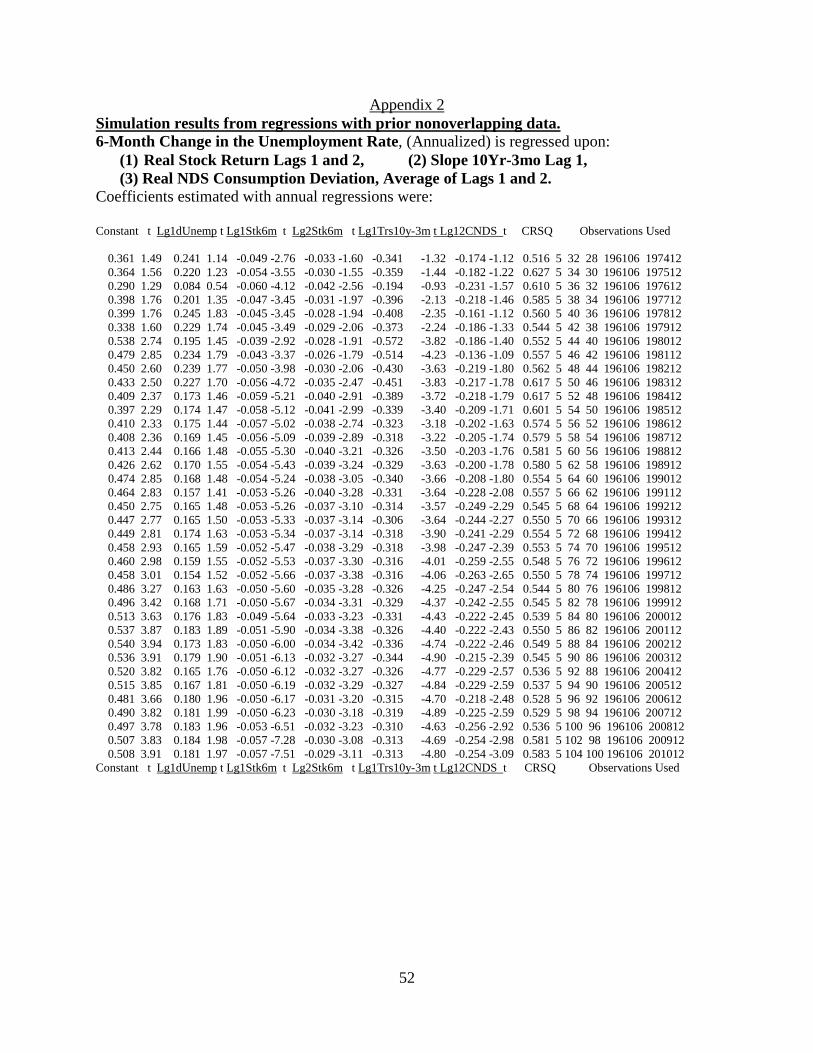
52
Appendix 2 Simulation results from regressions with prior nonoverlapping data. 6-Month Change in the Unemployment Rate, (Annualized) is regressed upon:
(1) Real Stock Return Lags 1 and 2, (2) Slope 10Yr-3mo Lag 1, (3) Real NDS Consumption Deviation, Average of Lags 1 and 2.
Coefficients estimated with annual regressions were: Constant t Lg1dUnemp t Lg1Stk6m t Lg2Stk6m t Lg1Trs10y-3m t Lg12CNDS t CRSQ Observations Used 0.361 1.49 0.241 1.14 -0.049 -2.76 -0.033 -1.60 -0.341 -1.32 -0.174 -1.12 0.516 5 32 28 196106 197412 0.364 1.56 0.220 1.23 -0.054 -3.55 -0.030 -1.55 -0.359 -1.44 -0.182 -1.22 0.627 5 34 30 196106 197512 0.290 1.29 0.084 0.54 -0.060 -4.12 -0.042 -2.56 -0.194 -0.93 -0.231 -1.57 0.610 5 36 32 196106 197612 0.398 1.76 0.201 1.35 -0.047 -3.45 -0.031 -1.97 -0.396 -2.13 -0.218 -1.46 0.585 5 38 34 196106 197712 0.399 1.76 0.245 1.83 -0.045 -3.45 -0.028 -1.94 -0.408 -2.35 -0.161 -1.12 0.560 5 40 36 196106 197812 0.338 1.60 0.229 1.74 -0.045 -3.49 -0.029 -2.06 -0.373 -2.24 -0.186 -1.33 0.544 5 42 38 196106 197912 0.538 2.74 0.195 1.45 -0.039 -2.92 -0.028 -1.91 -0.572 -3.82 -0.186 -1.40 0.552 5 44 40 196106 198012 0.479 2.85 0.234 1.79 -0.043 -3.37 -0.026 -1.79 -0.514 -4.23 -0.136 -1.09 0.557 5 46 42 196106 198112 0.450 2.60 0.239 1.77 -0.050 -3.98 -0.030 -2.06 -0.430 -3.63 -0.219 -1.80 0.562 5 48 44 196106 198212 0.433 2.50 0.227 1.70 -0.056 -4.72 -0.035 -2.47 -0.451 -3.83 -0.217 -1.78 0.617 5 50 46 196106 198312 0.409 2.37 0.173 1.46 -0.059 -5.21 -0.040 -2.91 -0.389 -3.72 -0.218 -1.79 0.617 5 52 48 196106 198412 0.397 2.29 0.174 1.47 -0.058 -5.12 -0.041 -2.99 -0.339 -3.40 -0.209 -1.71 0.601 5 54 50 196106 198512 0.410 2.33 0.175 1.44 -0.057 -5.02 -0.038 -2.74 -0.323 -3.18 -0.202 -1.63 0.574 5 56 52 196106 198612 0.408 2.36 0.169 1.45 -0.056 -5.09 -0.039 -2.89 -0.318 -3.22 -0.205 -1.74 0.579 5 58 54 196106 198712 0.413 2.44 0.166 1.48 -0.055 -5.30 -0.040 -3.21 -0.326 -3.50 -0.203 -1.76 0.581 5 60 56 196106 198812 0.426 2.62 0.170 1.55 -0.054 -5.43 -0.039 -3.24 -0.329 -3.63 -0.200 -1.78 0.580 5 62 58 196106 198912 0.474 2.85 0.168 1.48 -0.054 -5.24 -0.038 -3.05 -0.340 -3.66 -0.208 -1.80 0.554 5 64 60 196106 199012 0.464 2.83 0.157 1.41 -0.053 -5.26 -0.040 -3.28 -0.331 -3.64 -0.228 -2.08 0.557 5 66 62 196106 199112 0.450 2.75 0.165 1.48 -0.053 -5.26 -0.037 -3.10 -0.314 -3.57 -0.249 -2.29 0.545 5 68 64 196106 199212 0.447 2.77 0.165 1.50 -0.053 -5.33 -0.037 -3.14 -0.306 -3.64 -0.244 -2.27 0.550 5 70 66 196106 199312 0.449 2.81 0.174 1.63 -0.053 -5.34 -0.037 -3.14 -0.318 -3.90 -0.241 -2.29 0.554 5 72 68 196106 199412 0.458 2.93 0.165 1.59 -0.052 -5.47 -0.038 -3.29 -0.318 -3.98 -0.247 -2.39 0.553 5 74 70 196106 199512 0.460 2.98 0.159 1.55 -0.052 -5.53 -0.037 -3.30 -0.316 -4.01 -0.259 -2.55 0.548 5 76 72 196106 199612 0.458 3.01 0.154 1.52 -0.052 -5.66 -0.037 -3.38 -0.316 -4.06 -0.263 -2.65 0.550 5 78 74 196106 199712 0.486 3.27 0.163 1.63 -0.050 -5.60 -0.035 -3.28 -0.326 -4.25 -0.247 -2.54 0.544 5 80 76 196106 199812 0.496 3.42 0.168 1.71 -0.050 -5.67 -0.034 -3.31 -0.329 -4.37 -0.242 -2.55 0.545 5 82 78 196106 199912 0.513 3.63 0.176 1.83 -0.049 -5.64 -0.033 -3.23 -0.331 -4.43 -0.222 -2.45 0.539 5 84 80 196106 200012 0.537 3.87 0.183 1.89 -0.051 -5.90 -0.034 -3.38 -0.326 -4.40 -0.222 -2.43 0.550 5 86 82 196106 200112 0.540 3.94 0.173 1.83 -0.050 -6.00 -0.034 -3.42 -0.336 -4.74 -0.222 -2.46 0.549 5 88 84 196106 200212 0.536 3.91 0.179 1.90 -0.051 -6.13 -0.032 -3.27 -0.344 -4.90 -0.215 -2.39 0.545 5 90 86 196106 200312 0.520 3.82 0.165 1.76 -0.050 -6.12 -0.032 -3.27 -0.326 -4.77 -0.229 -2.57 0.536 5 92 88 196106 200412 0.515 3.85 0.167 1.81 -0.050 -6.19 -0.032 -3.29 -0.327 -4.84 -0.229 -2.59 0.537 5 94 90 196106 200512 0.481 3.66 0.180 1.96 -0.050 -6.17 -0.031 -3.20 -0.315 -4.70 -0.218 -2.48 0.528 5 96 92 196106 200612 0.490 3.82 0.181 1.99 -0.050 -6.23 -0.030 -3.18 -0.319 -4.89 -0.225 -2.59 0.529 5 98 94 196106 200712 0.497 3.78 0.183 1.96 -0.053 -6.51 -0.032 -3.23 -0.310 -4.63 -0.256 -2.92 0.536 5 100 96 196106 200812 0.507 3.83 0.184 1.98 -0.057 -7.28 -0.030 -3.08 -0.313 -4.69 -0.254 -2.98 0.581 5 102 98 196106 200912 0.508 3.91 0.181 1.97 -0.057 -7.51 -0.029 -3.11 -0.313 -4.80 -0.254 -3.09 0.583 5 104 100 196106 201012 Constant t Lg1dUnemp t Lg1Stk6m t Lg2Stk6m t Lg1Trs10y-3m t Lg12CNDS t CRSQ Observations Used

53
Out of Sample Forecast Errors and Implied R2 By Decade: BegDec EndDec Nobs HistMean ModelRMSE ImpRsq 1970 1979 10 1.396 1.011 0.475 1980 1989 20 1.604 1.088 0.540 1990 1999 20 0.849 0.743 0.233 2000 2009 20 1.506 0.878 0.660 2010 2019 3 0.689 0.316 0.790 Entire Forecast Period: Root mean squared forecast error = 0.912 Entire Forecast Period: RMSE using historic mean as forecast = 1.345 Entire Forecast Period: Implied R-Squared of Forecast = 0.541 Properties of Simulation fits and errors for observations: 33 to 105 ( 197506 to 201106 ) Dependent variable = Change in Unemployment Rate x2: t = t+0m to t=t+6mo VARIABLE COEFFICIENT STD ERROR T-STAT (OLS) Constant 0.1909 0.1063 1.80 Fitted 0.9387 0.0997 9.41 RSQ = 0.555 Durbin Watson = 1.76 CRSQ = 0.549 Autocorrel = 0.117 STD ERR = 0.8995 STD DEV (Y) = 1.3392 Observs = 197506 to 201106 Nobs = 73 Deg of freedom = 71