breaking the minsky{papert barrier for
TRANSCRIPT
BREAKING THE MINSKY–PAPERT BARRIER FORCONSTANT-DEPTH CIRCUITS∗
ALEXANDER A. SHERSTOV†
Abstract. The threshold degree of a Boolean function f is the minimum degree of a realpolynomial p that represents f in sign: f(x) ≡ sgn p(x). In a seminal 1969 monograph, Minsky andPapert constructed a polynomial-size constant-depth ∧,∨-circuit in n variables with thresholddegree Ω(n1/3). This lower bound underlies some of today’s strongest results on constant-depthcircuits. It has since been an open problem (O’Donnell and Servedio, STOC 2003) to improveMinsky and Papert’s bound to nΩ(1)+1/3.
We give a detailed solution to this problem. For any fixed k > 1, we construct an ∧,∨-formulaof size n and depth k with threshold degree Ω(n(k−1)/(2k−1)). This lower bound nearly matches aknown O(
√n) upper bound for arbitrary formulas, and is exactly tight for “regular” formulas. Our
result proves a conjecture due to O’Donnell and Servedio (STOC 2003) and a different conjecture dueto Bun and Thaler (2013). Applications to communication complexity and computational learningare given.
Key words. Polynomial representations of Boolean functions, polynomial threshold functions,threshold degree, computational learning theory, communication complexity theory, polynomial ap-proximation theory
AMS subject classifications. 03D15, 68Q15, 68Q17
1. Introduction. Let f : 0, 1n → 0, 1 be a given Boolean function. A realpolynomial p is said to represent f in sign if
sgn p(x) =
−1 if f(x) = 0,
+1 if f(x) = 1,
for every input x ∈ 0, 1n. The main complexity measure of interest is the degree ofp. The minimum degree of a sign-representing polynomial for f is called the thresholddegree of f , denoted deg±(f). This notion was introduced in 1969 in the seminalwork of Minsky and Papert [34], who proved that the parity function on n variableshas threshold degree n and examined the threshold degree of several other functions.Sign-representing polynomials quickly found a variety of applications in theoreticalcomputer science, the first of which were size-depth trade-offs [37, 53] and lowerbounds [29, 30] for various types of threshold circuits, oracle separations [4] for PP,and the famous proof that PP is closed under intersection [8].
Sign-representing polynomials have been especially useful in the study of constant-depth circuits, leading to algorithmic and complexity-theoretic breakthroughs in thearea. One such example is the fastest known algorithm for learning DNF formulas,due to Klivans and Servedio [25], with running time expO(n1/3). The authorsof [25] obtained their algorithm by proving an upper bound of O(n1/3 log n) on thethreshold degree of polynomial-size DNF formulas, essentially matching a classic lowerbound due to Minsky and Papert [34]. Another success story is the fastest knownalgorithm for learning read-once formulas, due to Ambainis et al. [3], with runningtime expO(
√n). That algorithm, too, follows from an upper bound of O(
√n)
∗Submitted to the editors April 8, 2015. An extended abstract of this paper appeared in Proceed-ings of the Forty-Sixth Annual ACM Symposium on Theory of Computing, pages 223–232, 2014.
Funding: The author was supported in part by NSF CAREER award CCF-1149018 and anAlfred P. Sloan Foundation Research Fellowship.†University of California, Los Angeles, CA 90095 ([email protected]).
2 ALEXANDER A. SHERSTOV
on the threshold degree of read-once formulas, obtained in a series of breakthroughpapers [36, 15, 3, 32] by learning theorists and quantum researchers.
Sign-representing polynomials have been equally influential in the complexity-theoretic study of constant-depth circuits. Recall that AC0 denotes the class of∧,∨,¬-circuits of constant depth and polynomial size. Aspnes et al. [4] used thenotion of threshold degree and its relaxations to give an ingenious new proof that AC0
circuits cannot compute or even approximate the parity function. Another contribu-tion [42, 43] in which threshold degree played a central role is the first construction ofan AC0 circuit with exponentially small discrepancy and hence maximum communica-tion complexity in nearly every model. This discrepancy result was used in [42] to showthe optimality of Allender’s classic simulation of AC0 functions by majority circuits,solving the open problem [29] on the relation between these two circuit classes. Sub-sequent work generalized the threshold degree method of [42, 43] to communicationmodels with three or more parties, resolving well-known questions [33, 14, 6, 50, 49]in communication complexity and circuit complexity. Yet another example of the useof threshold degree in complexity theory is the first exponential lower bound on thesign-rank of AC0 circuits [40], posed as a challenge by Babai et al. [5] twenty-two yearsearlier.
1.1. Our results. In light of these algorithmic and complexity-theoretic appli-cations, the problem of determining the threshold degree of constant-depth circuitshas attracted considerable attention. Forty-five years ago, Minsky and Papert [34]proved an Ω(n1/3) lower bound on the threshold degree of the constant-depth circuit
f(x) =
n1/3∧i=1
n2/3∨j=1
xij .
The only subsequent progress was a lower bound of Ω(n1/3 logk n) for an arbitraryconstant k, due to O’Donnell and Servedio [36]. In other words, it has been opensince 1969 to obtain a polynomial improvement on Minsky and Papert’s lower bound.We give a detailed solution to this problem. Our main result is as follows:
Theorem 1.1. Let k > 1 be any fixed integer. Define f : 0, 1n → 0, 1 by
f = NORn
12k−1
NORn
22k−1
· · · NORn
22k−1︸ ︷︷ ︸
k−1
.
Thendeg±(f) = Ω
(nk−12k−1
).
As usual, the symbol denotes function composition. Thus, the function f above is adepth-k tree of NOR gates, with top fan-in n1/(2k−1) and all other fan-ins n2/(2k−1).Recall that by De Morgan’s law, a tree of NOR gates is equivalent to a tree of alter-nating AND and OR gates of the same depth and size. For typesetting convenience,we work with NOR trees throughout this manuscript.
Several remarks are in order. For depth k = 2, Theorem 1.1 gives a new andentirely different proof of Minsky and Papert’s classic Ω(n1/3) lower bound. Fordepth k = 3, Theorem 1.1 proves a conjecture of O’Donnell and Servedio [36] whoproposed the function ANDn1/5 ORn2/5 ANDn2/5 as a candidate for threshold degreeΩ(n2/5). Finally, the lower bound of Theorem 1.1 is essentially optimal. As k grows,the bound approaches Ω(
√n), nearly matching a well-known O(
√n) upper bound on
BREAKING THE MINSKY–PAPERT BARRIER 3
the threshold degree of arbitrary read-once Boolean formulas [32]. Moreover, we showthat for any fixed depth k, the lower bound of Theorem 1.1 is tight for a large classBoolean formulas:
Theorem 1.2. Let k > 1 be any fixed integer. Define f : 0, 1n → 0, 1 by
f = NORn1NORn2
· · · NORnk ,
where n1, n2, . . . , nk are arbitrary integers with n1n2 · · ·nk = n. Then
deg±(f) = O(nk−12k−1 log n
).
Our techniques allow us to prove another conjecture on the threshold degreeof constant-depth circuits. The element distinctness function EDn : 0, 1ndlogne →0, 1 is given by
EDn(x) =∧
i,j=1,2,...,n:i 6=j
dlogne∨k=1
xi,k ⊕ xj,k.
Viewing the arguments to EDn as dlog ne-bit integers, the function evaluates to trueif and only if these n integers are pairwise distinct. A moment’s reflection revealsthat EDn is a CNF formula of polynomial size. Bun and Thaler [13] proposed thecomposed function ORn2/5 EDn3/5 as another candidate for threshold degree Ω(n2/5),a conjecture that we prove in this paper:
Theorem 1.3. Consider the depth-3 polynomial-size ∧,∨-circuit f given by
f = ORn2/5 EDn3/5 .
Thendeg±(f) > Ω(n2/5).
The lower bound in this theorem is optimal up to a logarithmic factor. This function isquite different from the corresponding construction of Theorem 1.1 for depth k = 3.Remarkably, the threshold degree in both cases turns out to be the same up to alogarithmic factor: Ω(n2/5) versus Ω(n/ log n)2/5, where n denotes the total numberof variables.
1.2. Further applications. Lower bounds on the threshold degree translate ina black-box manner into various lower bounds in computational learning theory andcommunication complexity. We focus on two illustrative applications in these researchareas. By the pattern matrix method [42, 43, 50, 49], Theorem 1.1 gives an improvedconstruction of a constant-depth circuit with exponentially small discrepancy:
Theorem 1.4. For every ε > 0, there is an (explicitly given) two-party commu-nication problem f : 0, 1n × 0, 1n → 0, 1, representable by a read-once ∧,∨-formula of constant depth, with discrepancy
disc(f) 6 exp(−Ω
(n
12−ε)).
The best previous upper bound was exp(−Ω(n/ log n)2/5), due to Bun and Thaler [13],preceded by an upper bound of exp(−Ω(n1/3)) due to Buhrman et al. [11] andSherstov [42, 43]. By the results of [50, 49], Theorem 1.4 generalizes to three ormore parties.
4 ALEXANDER A. SHERSTOV
As a second application, we consider the notions of threshold weight and thresholddensity, defined for a given Boolean function f : 0, 1n → 0, 1 as the minimumsize of a majority-of-parity and threshold-of-parity circuit for f , respectively. Bothquantities play a prominent role in computational learning theory. By the black-boxreduction in [29], Theorem 1.1 in this paper implies:
Theorem 1.5. For every ε > 0, there is an (explicitly given) read-once ∧,∨-formula f : 0, 1n → 0, 1 of constant depth with threshold weight and thresholddensity
exp(
Ω(n
12−ε))
.
Prior to Theorem 1.5, the best lower bounds for circuits of constant depth wereas follows: exp(Ω(n/ log n)2/5) for threshold weight, due to Bun and Thaler [13], andexp(Ω(n1/3)) for threshold density, due to Krause and Pudlak [29]. We defer a detailedexposition of these and other applications to Section 8.
1.3. Proof overview. Sign-representation is a particularly powerful analyticmodel, which explains the difficulty of proving lower bounds on the threshold degree.A much weaker model is that of uniform approximation, whereby a real polynomialrepresents a Boolean function f if it approximates f pointwise within 1/3, ranging in[−1/3, 1/3] on f−1(0) and in [2/3, 4/3] on f−1(1). Central to our proof is a hybridmodel, best thought of as one-sided approximation [16, 12, 45, 13], in which therepresenting polynomial ranges in [−1/3, 1/3] on f−1(0) and in [2/3,+∞) on f−1(1).The complexity measure of a Boolean function f in each of these cases is the minimumdegree of a real polynomial that represents f : the threshold degree, approximatedegree, and one-sided approximate degree of f, respectively.
We obtain our results by proving the following more general statement.
Theorem 1.6. Let f be an arbitrary Boolean function, with one-sided approxi-mate degree d. Then for all integers n, k > 0,
(1.1) deg±(NORcn NORcn2 · · · NORcn2︸ ︷︷ ︸k
f) > nk minn, d,
where c > 1 is an absolute constant.
Theorem 1.6 gives the best possible lower bound on the threshold degree of the com-position (1.1) in terms of the one-sided approximate degree of f. We consider thisresult to be of independent interest. It allows one to start with a function f that hashigh one-sided approximate degree—a weak notion of hardness—and transform it intoa vastly harder function, with high threshold degree. We deduce our lower bounds inTheorems 1.1 and 1.3 from Theorem 1.6 by letting f be either the NOR function orthe element distinctness function, for both of which the one-sided approximate degreeis known.
We give three different proofs of Theorem 1.6, one for arbitrary k and two simplerones for the special case k = 0. We describe all three below. While the main resultof this paper (Theorem 1.1) requires the full power of Theorem 1.6 for arbitrary k,the case k = 0 is already sufficient to prove an Ω(n2/5) lower bound on the thresholddegree of constant-depth circuits.
Proof for arbitrary k. The search for a sign-representing polynomial for agiven Boolean function f can be formulated as a linear program. By strong duality,the nonexistence of a sign-representing polynomial is therefore equivalent to the ex-istence of a certain dual object. This dual point of view has been influential in past
BREAKING THE MINSKY–PAPERT BARRIER 5
research [36, 42, 46, 44, 12, 45] and plays a central role in our paper as well. Putanother way, we prove Theorem 1.6 constructively, by exhibiting a feasible object inthe dual space. This object must be a nonzero function that agrees with f in signand is additionally orthogonal to low-degree polynomials.
The key challenge is ensuring the agreement in sign between the dual objectand the Boolean function f. This contrasts with simpler settings such as uniformapproximation, where the dual object is allowed to disagree with f on a small fractionof inputs. The vast majority of methods developed to date, including most recentlythe paper of Bun and Thaler [13], only work for uniform approximation.
We pursue a different approach. At a high level, the proof proceeds by inductionon circuit depth. For each depth, we do more than rule out a sign-representing poly-nomial—rather, we construct a pair of highly structured dual objects that imply highthreshold degree and additionally allow for induction. A recurring technique in thispaper is the construction of dual objects with desired analytic or metric propertiesby taking convex combinations of dual objects that almost have the desired proper-ties. The technical part of the paper includes intuitive descriptions at each level ofgranularity.
Proofs for k = 0. This case corresponds to compositions of the form NORn f,where f is an arbitrary Boolean function. Equivalently, we may speak of ORn fsince threshold degree is invariant under negation. We are able to fully characterizethe threshold degree of any such composition.
To build intuition for our result, suppose that∥∥∥∥f − p
q
∥∥∥∥∞<
1
2n,
where p and q are polynomials. Then ORn f is sign-represented by
n∑i=1
p(xi)
q(xi)− 1
2.
To obtain a sign-representing polynomial for ORn f, it suffices to multiply throughby the positive quantity
∏q(xi)
2. In summary, the threshold degree of ORn f is atmost deg p+ 2n deg q. This construction is due to Beigel et al. [8], who used it in aningenious way to prove the closure of PP under intersection. In previous work [46],we showed that this construction is optimal for n = 2, i.e., the threshold degree ofOR2 f equals (up to a small multiplicative constant) the least degree of a rationalfunction that approximates f pointwise. However, no characterization was known forgrowing n.
Observe that the above construction works even if p/q approximates f in a one-sided manner. In fact, we prove that this modified construction achieves the smallestpossible degree. Our proof works by manipulating a feasible solution to the dual ofthe one-sided rational approximation problem for f, in order to construct a feasiblesolution to the dual of the sign-representation problem for ORn f. The proof in thispaper is unrelated to the earlier work [46] for n = 2. As a corollary to the newlyobtained characterization of the threshold degree of ORn f, we recover the specialcase of Theorem 1.6 for k = 0.
We give yet another proof of Theorem 1.6 for k = 0 by combining our techniqueswith a construction due to Bun and Thaler [13]. Specifically, the authors of [13]proved that ORn f cannot be approximated uniformly within 1
2 − exp(−Ω(n)) by
6 ALEXANDER A. SHERSTOV
a polynomial of degree less than the one-sided approximate degree of f, a form ofhardness amplification for uniform approximation. In and of itself, that result doesnot imply anything about the threshold degree of ORn f. Indeed, there are examplesof functions [38, 39, 48] with threshold degree 1 that cannot be approximated uni-formly within 1
2 − exp(−Ω(n)) by a polynomial of degree cn for some constant c > 0.Nevertheless, we are able to adapt the techniques of this work to the setting of Bunand Thaler [13] and thereby obtain another proof of Theorem 1.6 for k = 0.
2. Preliminaries. We use the term Euclidean space to refer to Rn for somepositive integer n. Throughout this paper, Boolean functions are mappings X →0, 1 for some finite subset X of Euclidean space, most often X = 0, 1n. ForBoolean functions f : 0, 1n → 0, 1 and g : X → 0, 1, we let f g denote thecomponentwise composition of f with g, i.e., the Boolean function on Xn that sends(x1, x2, . . . , xn) 7→ f(g(x1), g(x2), . . . , g(xn)). By associativity, this definition extendsunambiguously to compositions f1 f2 · · · fk of three or more functions.
For a bit string x ∈ 0, 1n, we let |x| = x1 + x2 + · · · + xn denote the Ham-ming weight of x. The kth level of the Boolean hypercube 0, 1n is the subsetx ∈ 0, 1n : |x| = k. The notation log x refers to the logarithm of x to base 2.The negation of a Boolean function f : X → 0, 1 is denoted ¬f and defined as usualby (¬f)(x) = ¬f(x). The functions ANDn,ORn,NORn : 0, 1n → 0, 1 have theirstandard definitions:
ANDn(x) =
n∧i=1
xi, ORn(x) =
n∨i=1
xi, NORn = ¬ORn.
The element distinctness function EDn : (0, 1dlogne)n → 0, 1 is given by
EDn(x) =∧
i,j=1,2,...,n:i 6=j
dlogne∨k=1
xi,k ⊕ xj,k.
Viewing the arguments to EDn as dlog ne-bit integers, the function evaluates to trueif and only if these n integers are pairwise distinct. The sign function is denoted
sgn t =
−1 if t < 0,
0 if t = 0,
1 if t > 0.
For a multivariate real polynomial p : Rn → R, we let deg p denote the total degreeof p, i.e., the largest degree of any monomial of p. We use the terms degree and totaldegree interchangeably in this paper. The following simple but fundamental fact, dueto Minsky and Papert [34], allows one to transform a multivariate real polynomial on0, 1n into a related univariate real polynomial on 0, 1, 2, . . . , n without an increasein degree.
Proposition 2.1 (Minsky and Papert). Let p : 0, 1n → R be an arbitrary poly-nomial. Then the mapping
m 7→ Ex∈0,1n|x|=m
p(x) (m = 0, 1, 2, . . . , n)
is a univariate real polynomial of degree at most deg p.
We adopt the convention that 00 = 1, justified by continuity.
BREAKING THE MINSKY–PAPERT BARRIER 7
2.1. Norms and products. For a finite set X, we let RX denote the linearspace of functions f : X → R. This space is equipped with the usual norms and innerproduct:
‖f‖∞ = maxx∈X|f(x)|,
‖f‖1 =∑x∈X|f(x)|,
〈f, g〉 =∑x∈X
f(x)g(x).
The tensor product of f ∈ RX and g ∈ RY is the real function f ⊗ g ∈ RX×Ydefined by (f ⊗ g)(x, y) = f(x)g(y). The tensor product f ⊗ f ⊗ · · · ⊗ f (n times) isabbreviated f⊗n. The pointwise product of f, g ∈ RX is denoted f · g ∈ RX and isgiven by (f ·g)(x) = f(x)g(x). Note that as functions, f ·g is a restriction of f⊗g. Thesupport of a function f : X → R is denoted supp f = x ∈ X : f(x) 6= 0. A convexcombination of f1, f2, . . . , fk ∈ RX is any function of the form λ1f1+λ2f2+· · ·+λkfk,where λ1, λ2, . . . , λk are nonnegative and sum to 1. The convex hull of F ⊆ RX ,denoted convF, is the set of all convex combinations of functions in F.
For f : X → R, the symbols |f | and sgn f have their usual meanings as thereal functions given by |f |(x) = |f(x)| and (sgn f)(x) = sgn f(x). In the context offunctions, the relational operators 6,=, and > and arithmetic operations are appliedpointwise. For example, the phrase “f > 2|g| on X” means that f(x) > 2|g(x)| forevery x ∈ X.
Throughout this manuscript, we view probability distributions as real functions,which allows us to use the various notational devices introduced above. In particular,for probability distributions µ and λ, the symbol suppµ denotes the support of µ,and µ⊗λ denotes the probability distribution given by (µ⊗λ)(x, y) = µ(x)λ(y). If µis a probability distribution on X, we consider µ to be defined on any superset of Xwith the understanding that µ = 0 outside X.
2.2. Approximation by polynomials. Let f : X → 0, 1 be given, for a finitesubset X ⊂ Rn. The ε-approximate degree of f, denoted degε(f), is the least degreeof a real polynomial p such that ‖f − p‖∞ 6 ε. We refer to any such polynomial forf as a uniform approximant with error ε. Define
E(f, d) = minp:deg p6d
‖f − p‖∞,
where the minimum is over polynomials of degree at most d. In words, E(f, d) is theleast error to which f can be approximated by a real polynomial of degree no greaterthan d. In this notation, degε(f) = mind : E(f, d) 6 ε. In the study of Booleanfunctions, the standard setting of the error parameter is ε = 1/3.
Observe that deg1/2(f) = 0 for every Boolean function f , the approximant inquestion being the constant polynomial 1/2. While the 1/2-approximate degree of aBoolean function is always a trivial concept, the limit of the ε-approximate degree asε 1/2 turns out to be a fundamental and mathematically rich notion. It is knownas the threshold degree of f, denoted
deg±(f) = limε1/2
degε(f).
It is a simple but instructive exercise to verify that deg±(f) is precisely the least
8 ALEXANDER A. SHERSTOV
degree of a real polynomial p that represents f in sign:
sgn p(x) =
−1 if f(x) = 0,
+1 if f(x) = 1.
Clearly,
deg±(f) 6 degε(f), 0 6 ε <1
2.
Key to our work is a hybrid notion of approximation whereby a Boolean functionf is approximated uniformly on f−1(0) and represented in sign on f−1(1). Formally,the one-sided ε-approximate degree of f, denoted deg+
ε (f), is the least degree of a realpolynomial p such that
f(x)− ε 6 p(x) 6 f(x) + ε, x ∈ f−1(0),
f(x)− ε 6 p(x), x ∈ f−1(1).
We refer to any such polynomial for f as a one-sided approximant with error ε.Again, the canonical setting of the error parameter is ε = 1/3. Threshold degree andε-approximate degree are invariant under function negation:
deg±(f) = deg±(¬f),(2.1)
degε(f) = degε(¬f)(2.2)
for every Boolean function f and every ε. In contrast, the gap between the one-sidedapproximate degree of a Boolean function f : 0, 1n → R versus its negation ¬f canbe as large as 1 versus Ω(
√n), achieved for f = ORn.
We will need tight bounds on the one-sided approximate degree of several func-tions. The following theorem, due to Nisan and Szegedy [35], was one of the firstresults in this line of work.
Theorem 2.2 (Nisan and Szegedy).
deg1/3(NORn) = Θ(√n),
deg+1/3(NORn) = Θ(
√n).
The following result, obtained recently by Bun and Thaler [13, Appendix A], gen-eralizes earlier work [1, 2] on the approximate degree of element distinctness to theone-sided case.
Theorem 2.3 (Bun and Thaler).
deg+1/3(EDn) = Ω(n2/3).
2.3. Dual characterizations. Each of the approximation-theoretic notions re-viewed in the previous section has a dual characterization, obtained by an appeal tolinear programming duality. For threshold degree, we have:
Theorem 2.4. Let f : X → 0, 1 be given. Then deg±(f) > d if and only ifthere exists ψ : X → R such that
(i) ψ(x) > 0 whenever f(x) = 1,(ii) ψ(x) 6 0 whenever f(x) = 0,
BREAKING THE MINSKY–PAPERT BARRIER 9
(iii) 〈ψ, p〉 = 0 for every polynomial p of degree less than d, and(iv) ψ 6≡ 0.
A convenient shorthand for (i) and (ii), which we use often, is (−1)1−fψ > 0. Werefer the reader to [4, 36, 46] for a proof of Theorem 2.4. Analogously, approximatedegree has the following dual characterization [43, 52]:
Theorem 2.5. Let f : X → 0, 1 be given. Then degε(f) > d if and only if thereexists ψ : X → R such that
(i) 〈f, ψ〉 > ε‖ψ‖1,(ii) 〈ψ, p〉 = 0 for every polynomial p of degree less than d.
Finally, the dual characterization of one-sided approximate degree is as follows [13].
Theorem 2.6. Let f : X → 0, 1 be given. Then deg+ε (f) > d if and only if
there exists ψ : X → R such that(i) 〈f, ψ〉 > ε‖ψ‖1,
(ii) 〈ψ, p〉 = 0 for every polynomial p of degree less than d, and(iii) ψ(x) > 0 whenever f(x) = 1.
The dual objects that arise in Theorems 2.4 to 2.6 share the following metric proper-ties.
Proposition 2.7. Let ψ : X → R be given with 〈ψ, 1〉 = 0. Then(i)
∑x:ψ(x)>0 |ψ(x)| = ‖ψ‖1/2,
(ii) ‖ψ‖∞ 6 ‖ψ‖1/2,(iii) 〈f, ψ〉 6 ‖ψ‖1/2 for every Boolean function f : X → 0, 1.
Proof. (i) We have∑x:ψ(x)>0
|ψ(x)| = 〈|ψ|+ ψ, 1〉2
=〈|ψ|, 1〉
2=‖ψ‖1
2.
(ii) For every x∗ ∈ X,
0 = |〈ψ, 1〉| > |ψ(x∗)| −∑x6=x∗
|ψ(x)| = 2|ψ(x∗)| − ‖ψ‖1.
(iii) Immediate from (i) since f ranges in 0, 1.Most proofs in this paper involve explicit constructions of dual objects ψ as in
Theorems 2.4 to 2.6. A common step in such constructions is verifying that a candi-date object ψ is orthogonal to polynomials of low degree. We will make frequent useof the following observation.
Proposition 2.8. Let n, k, d be nonnegative integers, where n > 1. Let ψ : X →R be a function on a finite subset X of Euclidean space such that
〈ψ, p〉 = 0
for every polynomial p of degree less than d. Let g : Xn → R be given by
g(x1, x2, . . . , xn) =∑
i1<i2<···<ik
gi1,i2,...,ik(xi1 , xi2 , . . . , xik),
for some functions gi1,i2,...,ik : Xk → R. Then
〈ψ⊗n · g, P 〉 = 0
for every polynomial P of degree less than (n− k)d.
10 ALEXANDER A. SHERSTOV
Proof. By linearity, it suffices to prove the proposition for factored polynomialsP (x1, x2, . . . , xn) =
∏ni=1 pi(xi). By hypothesis, the degrees of p1, p2, . . . , pn sum to
less than (n−k)d. In particular, every subset S ⊆ 1, 2, . . . , n of cardinality |S| > n−kobeys mini∈S deg pi < d and therefore∏
i∈S〈ψ, pi〉 = 0.
We conclude that
〈ψ⊗n · g, P 〉 =∑
i1<i2<···<ik
〈ψ⊗k · gi1,i2,...,ik , pi1 ⊗ pi2 ⊗ · · · ⊗ pik〉∏
i/∈i1,i2,...,ik
〈ψ, pi〉
= 0.
We will also need an explicit dual object for the NOR function, in the sense ofTheorem 2.6. There are known constructions of such objects, due to Spalek [54] andBun and Thaler [12], but we require additional properties not ensured by previouswork.
Theorem 2.9. Let ε be given, 0 < ε < 1. Then for some δ = δ(ε) > 0 and everyn > 2, there exists an (explicitly given) function ω : 0, 1, 2, . . . , n → R such that
ω(0) >1− ε
2· ‖ω‖1,
(−1)n+tω(t) >ε
4t2· ‖ω‖1 (t = 1, 2, . . . , n),
deg p <√δn =⇒ 〈ω, p〉 = 0.
The proof of this result is an adaptation of previous analyses [54, 12] and can be foundin Appendix A.
2.4. Robust polynomials. A natural approach to approximating a composedfunction f g is to approximate f and g separately and compose the resulting approx-imants. For this approach to work, the approximating polynomial for f needs to berobust to noise in the inputs, i.e., it needs to approximate f not only on the Booleanhypercube but also on any perturbation of a Boolean vector. The following resultfrom [47] gives an efficient procedure for making any polynomial robust to noise.
Theorem 2.10 (Sherstov). Let p : 0, 1n → [−1, 1] be a given polynomial. Thenfor every δ > 0, there is a polynomial probust : Rn → R of degree O(deg p+ log 1
δ ) suchthat
|p(x)− probust(x+ ε)| < δ
for every x ∈ 0, 1n and ε ∈ [−1/3, 1/3]n.
Note that the degree of the robust polynomial grows additively rather than multiplica-tively with the error parameter δ. This fact will play a crucial role in the next section,where we prove our upper bound on the threshold degree of constant-depth circuits.It follows from the above result that the approximate degree is always well-behavedunder function composition [47]:
Corollary 2.11 (Sherstov). Let f : 0, 1n → 0, 1 and g : X → 0, 1 begiven. Then
deg1/3(f g) 6 cdeg1/3(f) deg1/3(g)
for some absolute constant c > 0 independent of f, g, n.
BREAKING THE MINSKY–PAPERT BARRIER 11
3. The upper bound. Consider an AND-OR tree of depth k on n variables,in which the fan-in may vary from level to level but is the same for all gates at anygiven level. O’Donnell and Servedio [36] made the following ingenious observation ina footnote of their paper: either the product of the odd-level fan-ins is at most
√n or
the product of the even-level fan-ins is at most√n, which means that the standard
arithmetization of the AND-OR tree gives a sign-representing polynomial of degreeat most
√n.
While O’Donnell and Servedio’s construction falls short of achieving our desired
bound of O(nk−12k−1 log n), the trick of odd- versus even-level fan-ins plays an essential
role in our proof. The other key ingredient is work on robust approximation [47],which allows one to make a polynomial robust to noise with essentially no overheadin degree. We start by calculating the parameters in the above construction.
Lemma 3.1 (cf. O’Donnell and Servedio). Let f = NORnk NORnk−1 · · ·
NORn1, where n1n2 · · ·nk = n. Then
(3.1) E(f, n2n4n6 · · · ) 61
2− 1
2nn2n4n6···.
Proof. By working with the negation of f if necessary, we may assume that
f(x) = · · ·n3∨i3=1
n2∧i2=1
n1∨i1=1︸ ︷︷ ︸
k
xi1,i2,...,ik .
Consider the polynomial
p(x) = · · ·n3∑i3=1
n2∏i2=1
n1∑i1=1
xi1,i2,...,ik .
It is clear that deg p = n2n4n6 · · · . Moreover, f(x) = 0 forces p(x) = 0, whereasf(x) = 1 forces
1 6 p(x) 6 ((nn21 n3)
n4 n5)n6 . . . 6 nn2n4n6···.
Now (3.1) is immediate, the approximant in question being
1
2+
1
nn2n4n6···
(p(x)− 1
2
).
Equation (3.1) shows that O’Donnell and Servedio’s approach gives a uniform ap-proximant with reasonable accuracy, rather than just a sign-representing polynomial.Combining this fact with results on robust approximation, we obtain a robust sign-representing polynomial for the AND-OR tree:
Corollary 3.2. Let f = NORnk NORnk−1· · ·NORn1
, where n1n2 · · ·nk = n.Then there is a polynomial probust : Rn → R such that
(3.2) deg probust 6 (n2n4n6 · · · ) · c log n
for some absolute constant c > 0, and
(3.3) |f(x)− probust(x+ ε)| 6 1
2− 1
4nn2n4n6···
for every x ∈ 0, 1n and ε ∈ [−1/3, 1/3]n.
12 ALEXANDER A. SHERSTOV
Proof. By Lemma 3.1, there is a polynomial p : 0, 1n → [−2, 2] of degree atmost n2n4n6 · · · such that
‖f − p‖∞ 61
2− 1
2nn2n4n6···.
Invoking Theorem 2.10 with δ = 1/8nn2n4n6··· gives a polynomial probust : Rn → R ofdegree O(deg p+ log 1
δ ) such that
|p(x)− probust(x+ ε)| 6 1
4nn2n4n6···
for every x ∈ 0, 1n and ε ∈ [−1/3, 1/3]n. Now (3.2) and (3.3) are immediate.
We are now in a position to describe the final construction. We start by splittingthe NOR tree at some level into a top part and a bottom part. Next, we constructa robust sign-representing polynomial for the top part, and a uniform approximantwith error 1/3 for the bottom part. Finally, we compose the resulting polynomialsto obtain a sign-representing polynomial for the original tree. This approach is madeprecise in the following theorem.
Theorem 3.3. Let f = NORnk NORnk−1 · · · NORn1
, where n1n2 · · ·nk = n.Then
(3.4) deg±(f) 6 ck mini=0,1,...,k−1
√n1n2 · · ·ni ni+2ni+4ni+6 · · · log n,
for some absolute constant c > 1.
Proof. Fix i arbitrarily and write f = f ′ f ′′, where
f ′ = NORnk NORnk−1 · · · NORni+1
,
f ′′ = NORni NORni−1 · · · NORn1
.
Corollary 3.2 provides a polynomial p′robust of degree at most (ni+2ni+4ni+6 · · · ) ·c′ log n for some absolute constant c′ > 1 such that
(3.5) |f ′(x)− p′robust(x+ ε)| < 1
2
for every x ∈ 0, 1ni+1ni+2···nk and ε ∈ [−1/3, 1/3]ni+1ni+2···nk .On the other hand, Theorem 2.2 states that deg1/3(NORm) = O(
√m), whence
by Corollary 2.11 the 1/3-approximate degree of f ′′ does not exceed (c′′)i√n1n2 · · ·ni
for some absolute constant c′′ > 1. Fix a polynomial p′′ of that degree, with
(3.6) ‖f ′′ − p′′‖∞ 61
3.
By (3.5) and (3.6),
‖f ′ f ′′ − p′robust p′′‖∞ <1
2.
In summary, the threshold degree of f = f ′ f ′′ is at most the product of the degreesof p′robust and p′′, whence (3.4).
We have arrived at the main result of this section, which settles Theorem 1.2 fromthe Introduction.
BREAKING THE MINSKY–PAPERT BARRIER 13
Theorem 3.4. Let f = NORnk NORnk−1 · · · NORn1
, where n1n2 · · ·nk = n.Then
deg±(f) 6 ck · nk−12k−1 log n
for some absolute constant c > 1.
Proof. The idea is to carefully optimize the choice of i in the previous theorem, byreplacing the minimum with a geometric mean. Specifically, let c > 1 be the absoluteconstant from Theorem 3.3. Then
deg±(f)
ck log n6 mini=0,1,...,k−1
√n1n2 · · ·ni ni+2ni+4ni+6 · · ·
6 (n2n4n6 · · · )1
2k−1
k−1∏i=1
(√n1n2 · · ·ni ni+2ni+4ni+6 · · · )
22k−1 ,
where the second inequality is obtained by replacing the minimum with a weightedgeometric mean of the quantities involved. Raising both sides to the power 2k − 1and simplifying,(
deg±(f)
ck log n
)2k−1
6 (n2n4n6 · · · )
(k−1∏i=1
n1n2 · · ·ni
)(k−1∏i=1
n2i+2n2i+4n
2i+6 · · ·
)
=
k∏j=1
nj−1−2b j−1
2 cj
k∏j=1
nk−jj
k∏j=1
n2b j−1
2 cj
=
k∏j=1
nk−1j
= nk−1.
4. The lower bound. We prove our lower bound on the threshold degree ofconstant-depth circuits by induction on circuit depth. The notion of a dual pair,defined next, plays a central role in this inductive argument.
Definition 4.1. Let f : X → 0, 1 be given. A (d0, d1, ε)-dual pair for f is anypair of functions ψ0, ψ1 : X → R such that:
(i) 〈f, ψ1〉 > 1−ε2 ‖ψ1‖1,
(ii) ψ1(x) > 0 whenever f(x) = 1,(iii) 〈ψ1, p〉 = 0 for every polynomial p of degree less than d1,(iv) 〈ψ0, p〉 = 0 for every polynomial p of degree less than d0,(v)
ψ0(x)
= maxψ1(x), 0 if f(x) = 0,
∈ [−ε|ψ1(x)|, ε|ψ1(x)|] if f(x) = 1.
In the final property, the absolute value |ψ1(x)| can be replaced with ψ1(x) in view ofpart (ii). This definition is monotonic in ε, in the sense that a (d0, d1, ε)-dual pair is a(d0, d1, ε
′)-dual pair for every ε′ > ε. In our applications, we will always take ε = 1/3.Properties (i)–(iii) can be summarized by saying that the function f of interest
has one-sided 1−ε2 -approximate degree at least d1. The dual object ψ1 witnesses this
fact, in the sense of linear programming duality (Theorem 2.6). The key difficultyis that ψ1 need not always agree in sign with f : while such agreement is assured onf−1(1), there may well be inputs in f−1(0) on which ψ1 is positive. The role of the
14 ALEXANDER A. SHERSTOV
accompanying object ψ0 is to eliminate those errors without introducing new ones.For this to work efficiently, ψ0 needs to be orthogonal to polynomials of sufficientlyhigh degree d0. The challenge in our proof is to inductively construct new dual pairsfrom old ones, while ensuring sufficiently rapid growth of d0, d1.
The following lemma shows how we obtain our first dual pair. It corresponds tothe base case of the inductive argument.
Lemma 4.2. Let f : X → 0, 1 be a given Boolean function, deg+ε (f) > 0. Then
f has a (1,deg+ε (f), 1
2ε − 1)-dual pair.
Proof. Abbreviate d = deg+ε (f). By Theorem 2.6, there exists ψ1 : X → R such
that
〈f, ψ1〉 > ε‖ψ1‖1(4.1)
as well as
f(x) = 1 =⇒ ψ1(x) > 0,(4.2)
deg p < d =⇒ 〈ψ1, p〉 = 0.(4.3)
Define ψ0 : X → R by
ψ0(x) =
maxψ1(x), 0 if f(x) = 0,(
1− ‖ψ1‖12〈f, ψ1〉
)ψ1(x) if f(x) = 1.
With properties (4.1)–(4.3) already established, the proof will be complete once weshow that ∣∣∣∣1− ‖ψ1‖1
2〈f, ψ1〉
∣∣∣∣ 6 1
2ε− 1,(4.4)
〈ψ0, 1〉 = 0.(4.5)
By (4.3) and Proposition 2.7 (i), (iii),∑x:ψ1(x)>0
ψ1(x) =‖ψ1‖1
2,(4.6)
〈f, ψ1〉 6‖ψ1‖1
2.(4.7)
Now the upper bound (4.4) is immediate from (4.1) and (4.7). The remaining prop-erty (4.5) can be verified as follows:
〈ψ0, 1〉 =∑
x:f(x)=0
ψ0(x) +∑
x:f(x)=1
ψ0(x)
=∑
x:ψ1(x)>0
(1− f(x))ψ1(x) +∑x∈X
f(x)
(1− ‖ψ1‖1
2〈f, ψ1〉
)ψ1(x)
=∑
x:ψ1(x)>0
ψ1(x)
︸ ︷︷ ︸=‖ψ1‖1/2
−∑
x:ψ1(x)>0
f(x)ψ1(x)
︸ ︷︷ ︸=〈f,ψ1〉
+
(1− ‖ψ1‖1
2〈f, ψ1〉
)〈f, ψ1〉,
where the final calculations use (4.2) and (4.6).
BREAKING THE MINSKY–PAPERT BARRIER 15
The inductive step in our proof is realized by the following “amplification theorem,”which transforms a dual pair for a given function f into a dual pair for the composedfunction NOR(f, f, . . . , f).
Theorem 4.3. Let ε, δ ∈ (0, 1) be arbitrary. Let f : X → 0, 1 be any functionthat has a (d0, d1, ε)-dual pair, where d0, d1 > 1. Then the function
F = NORcn f
has a (minnd0, d1,minnd0,√nd1, δ)-dual pair, where c = c(ε, δ) > 0 is a constant
independent of f, n, d0, d1.
The proof of Theorem 4.3 is lengthy and technical, and we defer it to section 5.To complete our program, we need to bridge the notions of dual pairs and sign-representation. The following lemma does just that.
Lemma 4.4. Let f : X → 0, 1 be any function that has a (d0, d1, ε)-dual pair forsome 0 6 ε < 1. Then
deg±(f) > mind0, d1.
Proof. Let (ψ0, ψ1) be a (d0, d1, ε)-dual pair for f. By definition,
deg p < d0 =⇒ 〈ψ0, p〉 = 0,(4.8)
deg p < d1 =⇒ 〈ψ1, p〉 = 0,(4.9)
f(x) = 1 =⇒ ψ1(x) > 0,(4.10)
f(x) = 1 =⇒ |ψ0(x)| 6 ε|ψ1(x)|,(4.11)
f(x) = 0 =⇒ ψ0(x) = maxψ1(x), 0,(4.12)
〈f, ψ1〉 >1− ε
2‖ψ1‖1.(4.13)
Letting ψ = ψ1 − ψ0, we have
deg p < mind0, d1 =⇒ 〈ψ, p〉 = 0,(4.14)
f(x) = 1 =⇒ ψ(x) > 0,(4.15)
f(x) = 0 =⇒ ψ(x) 6 0,(4.16)
where the first item holds by (4.8) and (4.9), the second by (4.10) and (4.11), and thethird by (4.12). Finally, we claim that
ψ 6≡ 0.(4.17)
Indeed, (4.13) implies that ψ1 is not identically zero on f−1(1), whereas (4.11) ensuresthat sgnψ(x) = sgnψ1(x) on f−1(1). By (4.14)–(4.17) and Theorem 2.4, the proof iscomplete.
Combining the above three results, we arrive at the technical centerpiece of this paper,stated previously as Theorem 1.6 in the Introduction:
Theorem 4.5. Let f : X → 0, 1 be given. Then for all integers n, k > 0,
deg±(NORcn NORcn2 · · · NORcn2︸ ︷︷ ︸k
f) > nk minn,deg+1/3(f),
where c > 1 is an absolute constant, independent of f, n, k.
16 ALEXANDER A. SHERSTOV
Proof. Take c > 1 sufficiently large, and abbreviate m = minn, deg+1/3(f). We
need only consider the case m > 1, the lower bound being trivial otherwise. We claimthat for each k = 0, 1, 2, . . . , the function
NORcn2 · · · NORcn2︸ ︷︷ ︸k
f
has a (dmnk−1e,mnk, 1/2)-dual pair. This claim holds by induction on k, with thebase case k = 0 settled by Lemma 4.2 and the inductive step realized by Theorem 4.3.Applying Theorem 4.3 once more shows that the function
(4.18) NORcn NORcn2 · · · NORcn2︸ ︷︷ ︸k
f
has an (mnk,mnk, 1/2)-dual pair. It follows by Lemma 4.4 that the composition(4.18) has threshold degree at least mnk, as was to be shown.
Corollary 4.6. There exists an absolute constant c > 0 such that for all integersn, k > 0,
deg±(NORn NORn2 · · · NORn2︸ ︷︷ ︸k
) > (cn)k.
Proof. Immediate from Theorems 2.2 and 4.5.
This corollary settles our main result, stated as Theorem 1.1 in the Introduction.We note that all parts of our argument (Lemmas 4.2 and 4.4 and Theorems 2.2, 4.3and 4.5) are constructive in that they produce explicit solutions to corresponding duallinear programs. In particular, our proof produces an explicit dual object, in the senseof Theorem 2.4, that witnesses the lower bound in Corollary 4.6.
Corollary 4.7. For every Boolean function f : X → 0, 1 and every n > 1,
deg±(ORn f) > mincn,deg+1/3(f),
where c > 0 is an absolute constant. In particular,
deg±(ORn2/5 EDn3/5) = Ω(n2/5).
Proof. The first claim holds by taking k = 0 in Theorem 4.5 and recalling thatthreshold degree is invariant under function negation. The second claim is immediatefrom the first in light of Theorem 2.3.
This settles Theorem 1.3 from the Introduction. In sections 6 and 7 we will presenttwo alternate proofs of Corollary 4.7, completely different from the proof just given.In fact, we will fully characterize the threshold degree of ORn f for every f .
5. Proof of Theorem 4.3. The objective of this section is to prove Theorem 4.3(the “amplification theorem”), which transforms a dual pair for a given Boolean func-tion into a dual pair of higher degree for the composed function NOR(f, f, . . . , f). Westart by reviewing the notation and hypothesis of the theorem. We then introduceauxiliary dual objects and establish their properties. In the final subsection, we putthese ingredients together to obtain the desired dual pair.
BREAKING THE MINSKY–PAPERT BARRIER 17
5.1. Notation. We adopt verbatim the notation and hypothesis of Theorem 4.3.Specifically, f is an arbitrary Boolean function on a finite subset X of Euclidean space;the reals 0 < ε < 1 and 0 < δ < 1 are arbitrary parameters; and it is assumed that fhas a (d0, d1, ε)-dual pair (ψ0, ψ1), for some positive integers d0, d1. By definition,
deg p < d0 =⇒ 〈ψ0, p〉 = 0,(5.1)
deg p < d1 =⇒ 〈ψ1, p〉 = 0,(5.2)
f(x) = 1 =⇒ ψ1(x) > 0,(5.3)
f(x) = 1 =⇒ |ψ0(x)| 6 ε|ψ1(x)|,(5.4)
f(x) = 0 =⇒ ψ0(x) = maxψ1(x), 0,(5.5)
and
(5.6) 〈f, ψ1〉 >1− ε
2‖ψ1‖1.
A simple but vital consequence of (5.2) is that
(5.7) 〈ψ1, 1〉 = 0.
It follows from (5.6) that
(5.8) ψ1 6≡ 0,
whence by homogeneity we may assume that
(5.9) ‖ψ1‖1 = 1.
Define α by
(5.10) 〈f, ψ1〉 =1− α
2.
Then
(5.11) 0 6 α < ε,
where the upper bound is immediate from (5.6) and (5.9), whereas the lower boundholds by (5.7), (5.9), and Proposition 2.7 (iii).
The objective of the proof is to construct a dual pair (Ψ0,Ψ1) with sufficientlyhigh degrees for the Boolean function F : XN → 0, 1 given by
F = NORN f,
where N = cn for some constant c = c(ε, δ) > 0. The construction will proceed instages, shown schematically in Figure 5.1. The inputs to the construction, shadedin gray, are the function f, its dual pair (ψ0, ψ1), and the parameters n, ε, δ. Theseare combined to build more complex intermediate objects, resulting eventually in thedesired dual pair (Ψ0,Ψ1) for F. To be precise, the intermediate objects are functionfamilies, indexed by nonnegative integers as in ωn, Ld,Λ
Nk,m. Throughout the proof,
small letters (f, ψ0, ψ1, µ0, µ1, µ∗, p) are reserved for functions on X, whereas capitalletters (Ψ0,Ψ1, L,Λ, Λ, P, P0, P1) refer to functions on XN .
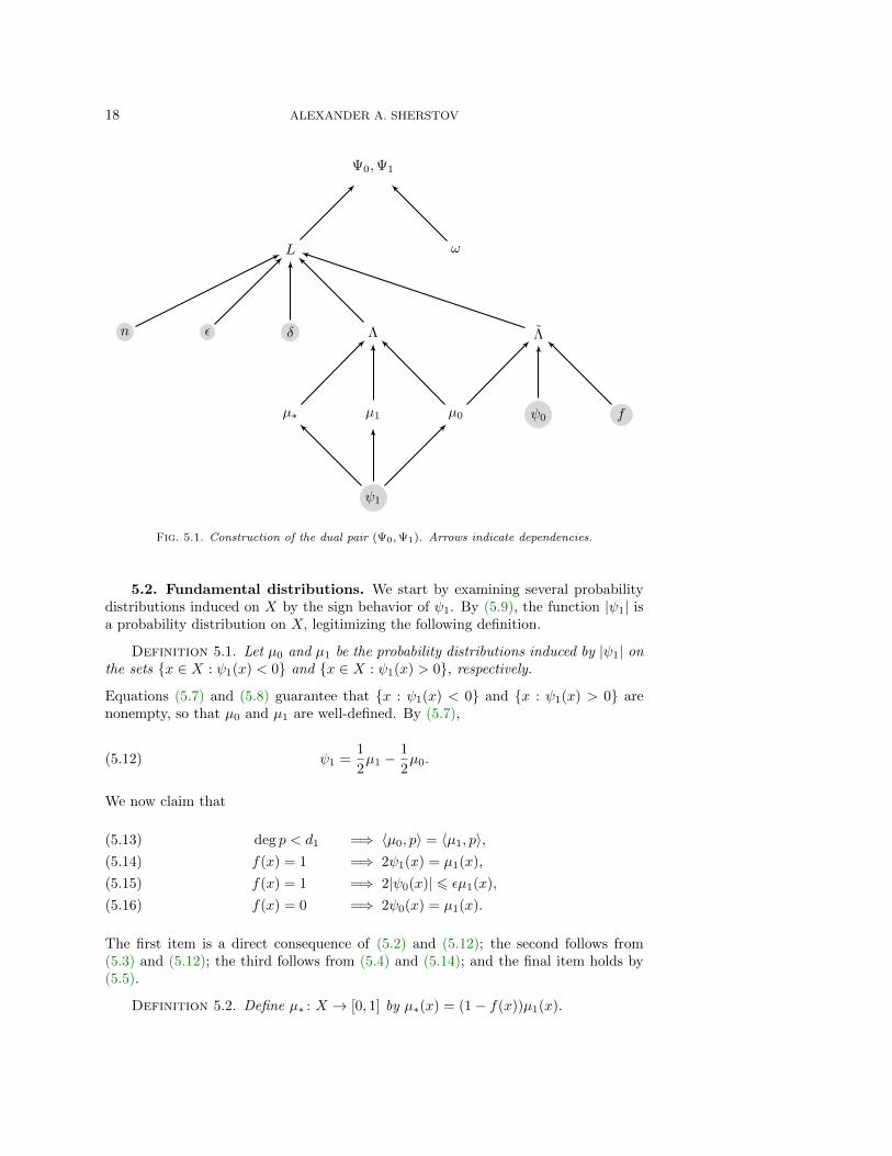
18 ALEXANDER A. SHERSTOV
ψ1
µ1 µ0µ∗ ψ0 f
Λ Λδεn
L ω
Ψ0,Ψ1
Fig. 5.1. Construction of the dual pair (Ψ0,Ψ1). Arrows indicate dependencies.
5.2. Fundamental distributions. We start by examining several probabilitydistributions induced on X by the sign behavior of ψ1. By (5.9), the function |ψ1| isa probability distribution on X, legitimizing the following definition.
Definition 5.1. Let µ0 and µ1 be the probability distributions induced by |ψ1| onthe sets x ∈ X : ψ1(x) < 0 and x ∈ X : ψ1(x) > 0, respectively.
Equations (5.7) and (5.8) guarantee that x : ψ1(x) < 0 and x : ψ1(x) > 0 arenonempty, so that µ0 and µ1 are well-defined. By (5.7),
ψ1 =1
2µ1 −
1
2µ0.(5.12)
We now claim that
deg p < d1 =⇒ 〈µ0, p〉 = 〈µ1, p〉,(5.13)
f(x) = 1 =⇒ 2ψ1(x) = µ1(x),(5.14)
f(x) = 1 =⇒ 2|ψ0(x)| 6 εµ1(x),(5.15)
f(x) = 0 =⇒ 2ψ0(x) = µ1(x).(5.16)
The first item is a direct consequence of (5.2) and (5.12); the second follows from(5.3) and (5.12); the third follows from (5.4) and (5.14); and the final item holds by(5.5).
Definition 5.2. Define µ∗ : X → [0, 1] by µ∗(x) = (1− f(x))µ1(x).
BREAKING THE MINSKY–PAPERT BARRIER 19
We have
〈1− f, µ1〉 = 1− 〈f, µ1〉= 1− 〈f, µ1 − µ0〉 since suppµ0 ⊆ f−1(0)
= 1− 2〈f, ψ1〉 by (5.12)
= α by (5.10),(5.17)
whence
(5.18) ‖µ∗‖1 = α.
We will need the following technical result from [45, Claim 3.3], which continues tohold with µ∗ replaced by any function.
Lemma 5.3. For every polynomial P : XN → R and every k = 0, 1, 2, . . . , N, themapping
z 7→
⟨µ⊗k∗ ⊗
N−k⊗i=1
µzi , P
⟩, z ∈ 0, 1N−k,(5.19)
is a polynomial of degree at most (degP )/d1.
Proof (adapted from [45]). By linearity, it suffices to consider factored polyno-mials of the form P (x1, . . . , xN ) = p1(x1) · · · pN (xN ). In this case (5.19) simplifiesto
z 7→k∏i=1
〈µ∗, pi〉 ·N−k∏i=1
〈µzi , pk+i〉, z ∈ 0, 1N−k.(5.20)
By (5.13), polynomials pi of degree less than d1 satisfy 〈µ0, pi〉 = 〈µ1, pi〉 and thereforedo not contribute to the degree of (5.20) as a real function on 0, 1N−k. It followsthat the degree of (5.20) is at most |i : deg pi > d1| 6 (degP )/d1.
5.3. Auxiliary objects in the tensor space. The fundamental distributionsµ0 and µ1 on X naturally give rise to the following family of functions ΛNk,m : XN →[0, 1].
Definition 5.4. For nonnegative integers k,m with k +m 6 N, define
(5.21) ΛNk,m(x1, x2, . . . , xN ) = ES,T
[∏i∈S
µ∗(xi) ·∏i∈T
µ1(xi) ·∏
i/∈S∪T
µ0(xi)
],
where the expectation is with respect to a uniformly random pair of disjoint sets S, T ⊆1, 2, . . . , N of size |S| = k and |T | = m.
We proceed to examine basic analytic and metric properties of ΛNk,m.
Lemma 5.5.(i) supp ΛNk,0 ⊆ F−1(1),
(ii) 〈ΛNk,m, 1〉 = ‖ΛNk,m‖1 = αk,
(iii) ΛNk,m = ΛNk′,m′ on F−1(1) whenever k +m = k′ +m′,
(iv) 〈F,ΛNk,m〉 = αk+m,
(v) ΛNk,m(x) 6= 0 only if |i : ψ1(xi) > 0| = k +m.

20 ALEXANDER A. SHERSTOV
Proof. (i) Immediate from the fact that suppµ0 ⊆ f−1(0) and suppµ∗ ⊆ f−1(0).(ii) The first equality holds because ΛNk,m is nonnegative, whereas the second is
immediate from the fact that the nonnegative functions µ0, µ1, µ∗ satisfy ‖µ0‖1 =‖µ1‖1 = 1 by definition and ‖µ∗‖1 = α by (5.18).
(iii) Recall that µ∗ = µ1 on f−1(0). Since F−1(1) = f−1(0)N , the claim follows.(iv) We have
〈F,ΛNk,m〉 = 〈F,ΛNk+m,0〉 by (iii)
= 〈1,ΛNk+m,0〉 by (i)
= αk+m by (ii).
(v) Immediate from the fact that suppµ∗ ⊆ suppµ1 = x ∈ X : ψ1(x) > 0 andsuppµ0 = x ∈ X : ψ1(x) < 0.
Lemma 5.6. For any polynomial P : XN → R, the mapping
m 7→ 〈ΛNk,m, P 〉 (m = 0, 1, 2, . . . , N − k)(5.22)
is a univariate polynomial of degree at most (degP )/d1.
Proof. For S ⊆ 1, 2, . . . , N with |S| = k, define
ΛNS,m(x) = ET
[∏i∈T
µ1(xi) ·∏
i/∈S∪T
µ0(xi)
]∏i∈S
µ∗(xi),
where the expectation is over a uniformly random subset T ⊆ 1, 2, . . . , N \ S ofcardinality |T | = m. It is clear that ΛNk,m = E|S|=k ΛNS,m, and therefore (5.22) is aconvex combination of mappings
m 7→ 〈ΛNS,m, P 〉 (m = 0, 1, 2, . . . , N − k)(5.23)
as S ranges over k-element subsets. As a result, the proof will be complete once weshow that (5.23) is a polynomial of degree at most (degP )/d1.
By symmetry, we may assume that S = 1, 2, . . . , k. By Lemma 5.3, the functionφ : 0, 1N−k → R given by
φ(z) =
⟨µ⊗k∗ ⊗
N−k⊗i=1
µzi , P
⟩
has degree at most (degP )/d1. Therefore by Proposition 2.1,
m 7→ Ez∈0,1N−k|z|=m
φ(z) (m = 0, 1, 2, . . . , N − k)(5.24)
is a univariate polynomial of degree at most (degP )/d1. It remains to note that theright-hand side of (5.24) is precisely 〈ΛNS,m, P 〉.
We now define a real function ΛN,rk that approximates ΛNk,0 pointwise and is addition-ally orthogonal to low-degree polynomials. The parameter r controls the accuracy ofthe approximation.
BREAKING THE MINSKY–PAPERT BARRIER 21
Definition 5.7. For integers k, r with 0 6 k 6 N and 0 6 r < k, defineΛN,rk : XN → R by
ΛN,rk (x) =2k
(k − r − 1)!E|S|=k
∏i∈S
ψ0(xi) ·k−r−1∏i=1
i−∑j∈S
f(xj)
·∏i/∈S
µ0(xi)
,(5.25)
where the expectation is over a uniformly random S ⊆ 1, 2, . . . , N of size |S| = k.
Lemma 5.8.
(i) 〈ΛN,rk , P 〉 = 0 for every polynomial P of degree less than (r + 1)d0,
(ii) ΛN,rk (x) 6= 0 only if |i : ψ1(xi) > 0| = k,
(iii) ΛN,rk = ΛN0,k on F−1(1),
(iv) |ΛN,rk | 6 εk−r(kr
)ΛN0,k on F−1(0).
Proof. (i) For t = 0, 1, 2, . . . , it follows from (5.1) that ψ0⊗t is orthogonal to every
polynomial of degree less than td0. Now Proposition 2.8 implies that the function
x 7→∏i∈S
ψ0(xi) ·k−r−1∏i=1
i−∑j∈S
f(xj)
·∏i/∈S
µ0(xi),
where S ⊆ 1, 2, . . . , N is a given subset, is orthogonal to every polynomial of degree
less than (|S| − (k − r − 1))d0. Since ΛN,rk is a linear combination of such functionswith |S| = k, the claim follows.
(ii) We have suppψ0 ⊆ x ∈ X : ψ1(x) > 0 by (5.3)–(5.5), and suppµ0 =x ∈ X : ψ1(x) < 0 by definition. The claim is now immediate from the definingequation, (5.25).
(iii) For every x ∈ F−1(1), we have f(xi) = 0 and 2ψ0(xi) = µ1(xi) for ev-ery i, where the former holds by definition and the latter by (5.16). Making thesesubstitutions in (5.25),
ΛN,rk (x) = E|S|=k
[∏i∈S
µ1(xi) ·∏i/∈S
µ0(xi)
]= ΛN0,k(x).
(iv) Fix any x with F (x) = 0. We claim that for every subset S ⊆ 1, 2, . . . , Nof size |S| = k,
(5.26)2k
(k − r − 1)!
∏i∈S|ψ0(xi)| ·
k−r−1∏i=1
∣∣∣∣∣∣i−∑j∈S
f(xj)
∣∣∣∣∣∣ ·∏i/∈S
µ0(xi)
6 εk−r(k
r
)∏i∈S
µ1(xi) ·∏i/∈S
µ0(xi).
To see this, consider the nonempty set A = i : f(xi) = 1. There are three possibil-ities.
• If A * S, then both sides of (5.26) vanish because µ0 is supported on f−1(0).
• If A ⊆ S and 1 6 |A| 6 k− r− 1, then∏k−r−1i=1 |i−
∑j∈S f(xj)| = 0 and the
left-hand side of (5.26) vanishes.
22 ALEXANDER A. SHERSTOV
• If A ⊆ S and k − r 6 |A| 6 k, then the left-hand side of (5.26) simplifies to(|A| − 1
k − r − 1
) ∏i∈S|2ψ0(xi)| ·
∏i/∈S
µ0(xi)
6
(k
r
)∏i∈S|2ψ0(xi)| ·
∏i/∈S
µ0(xi)
=
(k
r
)∏i∈A|2ψ0(xi)| ·
∏i∈S\A
|2ψ0(xi)| ·∏i/∈S
µ0(xi)
=
(k
r
)∏i∈A|2ψ0(xi)| ·
∏i∈S\A
µ1(xi) ·∏i/∈S
µ0(xi) by (5.16)
6
(k
r
)εk−r
∏i∈A
µ1(xi) ·∏
i∈S\A
µ1(xi) ·∏i/∈S
µ0(xi) by (5.15).
This completes the proof of (5.26). One now obtains |ΛN,rk (x)| 6 εk−r(kr
)ΛN0,k(x) by
passing to expectations on both sides of (5.26) with respect to a uniformly randomsubset S of cardinality k.
5.4. Simulating symmetric structure. The next step in our construction is afamily of real functions L1, L2, . . . , Lm, . . . with pairwise disjoint support whose roleis to mimic the levels of the Boolean hypercube, in the sense that inner product withLm roughly corresponds to the averaging operation on the mth level of the hypercube.In this way, we are able to simulate symmetric structure in a context with little actualsymmetry.
Let c′ = c′(δ) > 0 be a sufficiently large even integer. Then for each k =0, 1, 2, . . . , n, Theorem 2.9 gives an explicit function ωk : 0, 1, 2, . . . , c′n − k → Rsuch that
‖ωk‖1 = 1,(5.27)
ωk(0) >1
2− δ
12,(5.28)
|ωk(t)| > δ
24t2(t > 1),(5.29)
sgnωk(t) =
1 if t = 0,
(−1)k+t otherwise,(5.30)
deg p <√n =⇒ 〈ωk, p〉 = 0.(5.31)
By Proposition 2.7 (ii),
‖ωk‖∞ 61
2.(5.32)
We will work with the following integer parameters:
c′′ = min
c > 2 : εc−12cH(1/c) <
δ
20
,(5.33)
N = c′c′′n,(5.34)

BREAKING THE MINSKY–PAPERT BARRIER 23
where H is the binary entropy function. Observe that c′′ = c′′(ε, δ) > 0 is a constant.
Definition 5.9. Define L1, L2, . . . , Lc′n : XN → R by
Lm =
m−1∑k=0
(4
δ
)kωk(m− k)ΛNc′′k,c′′(m−k) (m 6 n),
Lm =
n∑k=0
(4
δ
)kωk(m− k)
(ΛNc′′k,c′′(m−k) − ΛN,nc′′m
)(m > n+ 1).
The following lemma collects key properties of this function family.
Lemma 5.10.(i) Lm(x) 6= 0 only if |i : ψ1(xi) > 0| = c′′m,
(ii) Lm = 0 on F−1(1) for every m > n+ 1,(iii) (−1)mLm > 0,
(iv) Lm =∑m−1k=0 (4/δ)kωk(m− k)ΛNc′′m,0 on F−1(1) for every m = 1, 2, . . . , n,
(v) ‖Lm‖1 =∑minm−1,nk=0 (4αc
′′/δ)k|ωk(m− k)|.
Proof. (i) Immediate from Lemma 5.5 (v) and Lemma 5.8 (ii).(ii) On F−1(1), we have the following identity for every k:
ΛNc′′k,c′′(m−k) − ΛN,nc′′m = ΛN0,c′′m − ΛN,nc′′m = 0,
where the first step uses Lemma 5.5 (iii), and the second Lemma 5.8 (iii). The claimis now immediate from the defining equation of Lm for m > n+ 1.
(iii) For m = 1, 2, . . . , n, the claim follows directly from (5.30) and the nonneg-ativity of ΛNc′′k,c′′(m−k). Consider now Lm for m > n + 1 and fix an arbitrary point
x ∈ suppLm. Then F (x) = 0 by (ii). As a result,
(5.35) |ΛN,nc′′m(x)| 6 εc′′m−n
(c′′m
n
)ΛN0,c′′m(x)
by Lemma 5.8 (iv). In light of (5.30), the defining equation of Lm for m > n+1 gives
(−1)mLm(x) =
n∑k=0
(4
δ
)k|ωk(m− k)|
(ΛNc′′k,c′′(m−k)(x)− ΛN,nc′′m(x)
)=
n∑k=1
(4
δ
)k|ωk(m− k)|ΛNc′′k,c′′(m−k)(x)
+
|ω0(m)|ΛN0,c′′m(x)−
n∑k=0
(4
δ
)k|ωk(m− k)|ΛN,nc′′m(x)
.
Using the estimates (5.29), (5.32), and (5.35), we arrive at
(−1)mLm(x) >n∑k=1
(4
δ
)k|ωk(m− k)|ΛNc′′k,c′′(m−k)(x)
+
δ
24m2−(
4
δ
)n· εc′′m−n
(c′′m
n
) ΛN0,c′′m(x).

24 ALEXANDER A. SHERSTOV
The terms in the summation are nonnegative. Thus, the proof will be complete oncewe show that the expression in braces is nonnegative as well, which is accomplishedby the following calculation:(
4
δ
)n· εc′′m−n
(c′′m
n
)6
(4
δ
)m−1· εc′′m−m
(c′′m
m
)since m > n+ 1 and c′′ > 2
6δ
4
(4
δ· εc′′−12c
′′H(1/c′′)
)m6
δ
4 · 5mby (5.33)
6δ
24m2since m > 2.
(iv) Immediate from Lemma 5.5 (iii).(v) For m = 1, 2, . . . , n,
‖Lm‖1 = 〈Lm, sgnLm〉= (−1)m〈Lm, 1〉 by (iii)
= (−1)mm−1∑k=0
(4
δ
)kωk(m− k)〈ΛNc′′k,c′′(m−k), 1〉
= (−1)mm−1∑k=0
(4αc
′′
δ
)kωk(m− k) by Lemma 5.5 (ii)
=
m−1∑k=0
(4αc
′′
δ
)k|ωk(m− k)| by (5.30).
The analysis for m > n+ 1 is similar but has an additional step:
‖Lm‖1 = 〈Lm, sgnLm〉= (−1)m〈Lm, 1〉 by (iii)
= (−1)mn∑k=0
(4
δ
)kωk(m− k)〈ΛNc′′k,c′′(m−k) − ΛN,nc′′m, 1〉
= (−1)mn∑k=0
(4
δ
)kωk(m− k)〈ΛNc′′k,c′′(m−k), 1〉 by Lemma 5.8 (i)
= (−1)mn∑k=0
(4αc
′′
δ
)kωk(m− k) by Lemma 5.5 (ii)
=n∑k=0
(4αc
′′
δ
)k|ωk(m− k)| by (5.30).
BREAKING THE MINSKY–PAPERT BARRIER 25
5.5. Constructing the dual objects. We are finally in a position to constructthe claimed dual pair (Ψ0,Ψ1) for F. Let
Ψ0 =∑
m=1,2,...,c′n:m even
Lm +
n∑m=0
(4
δ
)m(ωm(0)− 1
2
)ΛNc′′m,0,(5.36)
Ψ1 =
c′n∑m=1
Lm +
n∑m=0
(4
δ
)mωm(0)ΛNc′′m,0.(5.37)
The next two lemmas establish useful facts about these functions.
Lemma 5.11. There are Λ0, Λ1 ∈ spanΛN,nm : n+ 1 6 m 6 N such that
Ψ0 =n∑k=0
(4
δ
)k(ωk(0)− 1
2
)ΛNc′′k,0 +
∑m=1,2,...,c′n−k:m≡k (mod 2)
ωk(m)ΛNc′′k,c′′m
+ Λ0,
(5.38)
Ψ1 =
n∑k=0
(4
δ
)k c′n−k∑m=0
ωk(m)ΛNc′′k,c′′m + Λ1.
(5.39)
Proof. Substituting the defining equation for Lm in (5.36),
Ψ0 =∑
m=1,2,...,c′n:m even
minm−1,n∑k=0
(4
δ
)kωk(m− k)ΛNc′′k,c′′(m−k)
+
n∑m=0
(4
δ
)m(ωm(0)− 1
2
)ΛNc′′m,0 + Λ0
=
n∑k=0
∑m=1,2,...,c′n−k:m≡k (mod 2)
(4
δ
)kωk(m)ΛNc′′k,c′′m
+
n∑m=0
(4
δ
)m(ωm(0)− 1
2
)ΛNc′′m,0 + Λ0,
where Λ0 is as claimed in the lemma statement. Now (5.38) is immediate.The proof for Ψ1 is analogous. Substituting the defining equation for Lm in (5.37),
Ψ1 =
c′n∑m=1
minm−1,n∑k=0
(4
δ
)kωk(m− k)ΛNc′′k,c′′(m−k)
+
n∑m=0
(4
δ
)mωm(0)ΛNc′′m,0 + Λ1
=
c′n∑m=0
minm,n∑k=0
(4
δ
)kωk(m− k)ΛNc′′k,c′′(m−k) + Λ1,
26 ALEXANDER A. SHERSTOV
where Λ1 is as claimed in the lemma statement. The final expression is equivalentto (5.39) by basic algebra.
Lemma 5.12. On F−1(1), one has
Ψ0 =∑
m=0,1,...,n:m even
(−1
2
(4
δ
)m+
m∑k=0
(4
δ
)kωk(m− k)
)ΛNc′′m,0(5.40)
+∑
m=0,1,...,n:m odd
(4
δ
)m(ωm(0)− 1
2
)ΛNc′′m,0,
Ψ1 =
n∑m=0
(m∑k=0
(4
δ
)kωk(m− k)
)ΛNc′′m,0.(5.41)
Proof. For any input x with F (x) = 1,
Ψ0(x) =∑
m=1,2,...,c′n:m even
Lm(x) +
n∑m=0
(4
δ
)m(ωm(0)− 1
2
)ΛNc′′m,0(x)
=∑
m=1,2,...,n:m even
(m−1∑k=0
(4
δ
)kωk(m− k)
)ΛNc′′m,0(x)
+
n∑m=0
(4
δ
)m(ωm(0)− 1
2
)ΛNc′′m,0(x),
where the first equality holds by definition, and the second by Lemma 5.10 (ii), (iv).This proves (5.40).
The proof of (5.41) is closely analogous. For x ∈ F−1(1),
Ψ1(x) =
c′n∑m=1
Lm(x) +
n∑m=0
(4
δ
)mωm(0)ΛNc′′m,0(x)
=
n∑m=1
(m−1∑k=0
(4
δ
)kωk(m− k)
)ΛNc′′m,0(x) +
n∑m=0
(4
δ
)mωm(0)ΛNc′′m,0(x),
where the first equality holds by definition, and the second equality is valid byLemma 5.10 (ii), (iv).
We are now in a position to establish one by one the properties required of Ψ0,Ψ1 to bea dual pair for F. The five lemmas that follow, Lemmas 5.13 to 5.17, are independentand can be read in any order.
Lemma 5.13. 〈F,Ψ1〉 > 1−δ2 ‖Ψ1‖1.
BREAKING THE MINSKY–PAPERT BARRIER 27
Proof. We have
〈F,Ψ1〉 =
n∑m=0
m∑k=0
(4
δ
)kωk(m− k)〈F,ΛNc′′m,0〉 by (5.41)
=
n∑m=0
m∑k=0
(4
δ
)kωk(m− k)αc
′′m by Lemma 5.5 (iv)
=
n∑k=0
(4αc
′′
δ
)k n−k∑m=0
αc′′mωk(m) by basic algebra
>n∑k=0
(4αc
′′
δ
)k (ωk(0)− αc
′′‖ωk‖1
)
>
n∑k=0
(4αc
′′
δ
)k (1
2− δ
12− αc
′′)
by (5.27) and (5.28)
>n∑k=0
(4αc
′′
δ
)k1− δ
2by (5.11) and (5.33).
On the other hand,
‖Ψ1‖1 6c′n∑m=1
‖Lm‖1 +
n∑m=0
(4
δ
)m|ωm(0)|‖ΛNc′′m,0‖1 by (5.37)
=
c′n∑m=1
minm−1,n∑k=0
(4αc
′′
δ
)k|ωk(m− k)|
+
n∑m=0
(4αc
′′
δ
)m|ωm(0)| by Lemma 5.10(v) and 5.5(ii)
=
n∑k=0
(4αc
′′
δ
)k c′n−k∑m=0
|ωk(m)| by basic algebra
=
n∑k=0
(4αc
′′
δ
)kby (5.27).
Lemma 5.14. Ψ1(x) > 0 whenever F (x) = 1.
Proof. By (5.41), it suffices to show that(4
δ
)mωm(0) >
m−1∑k=0
(4
δ
)k|ωk(m− k)| (m = 0, 1, . . . , n).(5.42)
This relation follows directly from the properties of ωk. Specifically, by (5.28) theleft-hand side of (5.42) is at least (4/δ)m(1 − δ/6)/2 > (4/δ)m/3, whereas by (5.32)
the right-hand side of (5.42) is at most∑m−1k=0 (4/δ)k/2 6 (4/δ)m/6.
Lemma 5.15. Let P0, P1 : XN → R be polynomials with
degP0 < minnd0, d1,degP1 < minnd0,
√nd1.
28 ALEXANDER A. SHERSTOV
Then
〈Ψ0, P0〉 = 〈Ψ1, P1〉 = 0.
Proof. Lemma 5.6 ensures the existence of univariate polynomials p0, p1, . . . , pnsuch that
〈ΛNc′′k,m, P1〉 = pk(m) (k = 0, 1, . . . , n; m = 0, 1, . . . , N − c′′k),(5.43)
deg pk <√n (k = 0, 1, . . . , n).(5.44)
Thus,
〈Ψ1, P1〉 =
n∑k=0
(4
δ
)k c′n−k∑m=0
ωk(m)〈ΛNc′′k,c′′m, P1〉 by Lemma 5.11 and Lemma 5.8 (i)
=
n∑k=0
(4
δ
)k c′n−k∑m=0
ωk(m)pk(c′′m) by (5.43)
=
n∑k=0
(4
δ
)k· 0 by (5.31) and (5.44)
= 0.
We now prove the claim for Ψ0. By (5.27), (5.31), and Proposition 2.7 (i),
∑m:ωk(m)>0
ωk(m) =1
2
for every k, which in view of (5.30) is equivalent to
(5.45) ωk(0) +∑
m=1,2,...,c′n−k:m≡k (mod 2)
ωk(m) =1
2.
From this point on, the analysis is similar to the one above for Ψ1. By Lemma 5.6,there are reals a0, a1, . . . , an (i.e., zero-degree polynomials) such that
〈ΛNc′′k,m, P0〉 = ak (k = 0, 1, . . . , n; m = 0, 1, . . . , N − c′′k).(5.46)
BREAKING THE MINSKY–PAPERT BARRIER 29
By Lemma 5.11 and Lemma 5.8 (i),
〈Ψ0, P0〉 =
n∑k=0
(4
δ
)k(ωk(0)− 1
2
)〈ΛNc′′k,0, P0〉+
∑m=1,2,...,c′n−k:m≡k (mod 2)
ωk(m)〈ΛNc′′k,c′′m, P0〉
=
n∑k=0
(4
δ
)kωk(0)− 1
2+
∑m=1,2,...,c′n−k:m≡k (mod 2)
ωk(m)
ak by (5.46)
=
n∑k=0
(4
δ
)k· 0 by (5.45)
= 0.
Lemma 5.16. Ψ0 = maxΨ1, 0 on F−1(0).
Proof. Recall from Lemma 5.5 (i) that for any k, the support of ΛNk,0 is contained
in F−1(1). As a result, the defining equations (5.36) and (5.37) simplify on F−1(0) to
Ψ0 =∑
m=1,2,...,c′n:m even
Lm, Ψ1 =
c′n∑m=1
Lm.
This completes the proof since by Lemma 5.10 (i), (iii), the functions in questionL1, L2, . . . , Lm, . . . have pairwise disjoint support, with sgnLm = (−1)m on the sup-port of Lm.
Lemma 5.17. |Ψ0| 6 δΨ1 on F−1(1).
Proof. Recall from Lemma 5.5 (v) that the functions ΛNc′′m,0 for m = 0, 1, 2, . . . , nhave pairwise disjoint support. Therefore, the claimed result will follow immediatelyfrom Lemma 5.12 once we verify the inequality
(5.47) max
∣∣∣∣∣−1
2
(4
δ
)m+
m∑k=0
(4
δ
)kωk(m− k)
∣∣∣∣∣ ,(
4
δ
)m ∣∣∣∣12 − ωm(0)
∣∣∣∣
6 δ
m∑k=0
(4
δ
)kωk(m− k)
for every m = 0, 1, . . . , n. We have∣∣∣∣ωm(0)− 1
2
∣∣∣∣ 6 δ
12by (5.28) and (5.32),
|ωk(m− k)| 6 1
2by (5.32).
30 ALEXANDER A. SHERSTOV
Thus, the left-hand side of (5.47) is at most
(4
δ
)m ∣∣∣∣12 − ωm(0)
∣∣∣∣+
m−1∑k=0
(4
δ
)k|ωk(m− k)| 6
(4
δ
)m(δ
12+
δ
8− 2δ
)
6
(4
δ
)m−1,
whereas the right-hand side of (5.47) is at least
δ
(4
δ
)mωm(0)− δ
m−1∑k=0
(4
δ
)k|ωk(m− k)| > δ
(4
δ
)m(1
2− δ
12− δ
8− 2δ
)
>
(4
δ
)m−1.
Lemmas 5.13 to 5.17 establish that (Ψ0,Ψ1) is a (minnd0, d1,minnd0,√nd1, δ)-
dual pair for F. This completes the proof of Theorem 4.3.
5.6. Generalizations. The proof of Theorem 4.3 presented in this section canbe generalized in several ways. As a concrete example, define a generalized (d0, d1, ε)-dual pair for f : X → 0, 1 to be any pair of real functions ψ0, ψ1 : X → R suchthat
(i) 〈f, ψ1〉 > 1−ε2 ‖ψ1‖1,
(ii) ψ1(x) > 0 whenever f(x) = 1,(iii) 〈ψ1, p〉 = 0 for every polynomial p of degree less than d1,(iv) 〈ψ0, p〉 = 0 for every polynomial p of degree less than d0,(v)
ψ0(x) ∈
[ψ1(x), 2ψ1(x)] if f(x) = 0 and ψ1(x) > 0,
[−ε|ψ1(x)|, ε|ψ1(x)|] otherwise.
This definition extends the notion of a (d0, d1, ε)-dual pair from section 4. Indeed, re-quirements (i)–(iv) are unchanged but the final requirement (v) is significantly weakerthan before. It is not hard to adapt our proof of Theorem 4.3 to this alternate defi-nition of a dual pair, for a small absolute constant ε > 0.
6. A complete characterization of the threshold degree. In this section,we study composed functions of the form ORnf . We fully characterize the thresholddegree of any such composition in terms of an approximation-theoretic property of f.Specifically, we show that up to a logarithmic factor, the threshold degree of ORn ffor n > 2 equals
mind0,d1
nd0 + d1 ,
where the minimum is over all d0, d1 > 0 such that f can be approximated in aone-sided manner to within 1/3 by a rational function with denominator degree d0and numerator degree d1. As a limiting case, we show that the threshold degree ofORn f for n large essentially coincides with the one-sided approximate degree of f .The work in this section gives a different proof of Corollary 4.7.
6.1. One-sided rational approximation. Analogous to the one-sided approx-imation of Boolean functions by polynomials, reviewed in section 2, the definitionbelow formalizes one-sided approximation by rational functions.
BREAKING THE MINSKY–PAPERT BARRIER 31
Definition 6.1. For d0 > 0 and a Boolean function f : X → 0, 1, definedeg+
ε (f, d0) to be the smallest d1 > 0 for which there exist polynomials p0, p1 of degreeat most d0, d1, respectively, with
f(x) = 0 =⇒∣∣∣∣p1(x)
p0(x)
∣∣∣∣ 6 ε,
f(x) = 1 =⇒ p1(x)
p0(x)> 1− ε.
Implicit in this definition is the requirement that p0(x) 6= 0 for every x ∈ X. Since apolynomial can be viewed as a rational function with denominator degree 0, we have
deg+ε (f) = deg+
ε (f, 0).
There is a partial equivalence between one-sided and two-sided approximation byrational functions. Specifically, any one-sided rational approximant for f with denom-inator degree d0 and numerator degree d1 gives a two-sided (`∞-norm) approximantfor the same function with a numerator and denominator of degree at most 2d0 +2d1.This equivalence has no bearing on our paper because we treat numerator degree anddenominator degree as distinct complexity measures—indeed, our interest is preciselyin the trade-off between them. Nevertheless, we include a proof of this interestingfact for the sake of completeness.
Proposition 6.2. For every function f : X → 0, 1 and every 0 < ε < 1/2,
M 6 minp,q
deg p+ deg q :
∥∥∥∥f − p
q
∥∥∥∥∞
6 ε
6 4M,
whereM = min
d=0,1,2,...d+ deg+
ε (f, d).
Proof. The lower bound is trivial since one-sided approximation is a weaker re-quirement than approximation in the `∞ norm. In the other direction, fix an integerd > 0 and polynomials p0, p1 of degree at most d and deg+
ε (f, d), respectively, with|p1/p0| 6 ε on f−1(0) and p1/p0 > 1− ε on f−1(1). Letting
f =p21
p21 + ε(1− ε)p20,
we have 0 6 f 6 ε on f−1(0) and 1− ε 6 f 6 1 on f−1(1).
Analogous to polynomial approximation, there is a generic way to rapidly reduce theerror in a one-sided approximation by rational functions.
Proposition 6.3. For any function f : X → 0, 1 and any k = 1, 2, 3, . . . ,
deg+εk
εk+(1−ε)k(f, kd) 6 k deg+
ε (f, d).
Proof. Fix d > 0 and polynomials p0, p1 of degree at most d and deg+ε (f, d),
respectively, such that |p1/p0| 6 ε on f−1(0) and p1/p0 > 1 − ε on f−1(1). Lettingq0 = pk0 and q1 = pk1/(ε
k + (1− ε)k), we obtain∣∣∣∣q1q0∣∣∣∣ 6 εk
εk + (1− ε)kon f−1(0),
q1q0
> 1− εk
εk + (1− ε)kon f−1(1).
32 ALEXANDER A. SHERSTOV
A substantial disadvantage of one-sided approximate degree, in the setting of rationalfunctions, is its lack of a clean and exact dual characterization. We therefore considera closely related quantity that admits such a characterization.
Definition 6.4. For d0, d1 > 0 and a Boolean function f : X → 0, 1, defineR(f, d0, d1) as the infimum over all ε > 0 for which there exist polynomials p0, p1 ofdegree at most d0, d1, respectively, such that
f(x) = 0 =⇒ |p1(x)| < εp0(x),(6.1)
f(x) = 1 =⇒ |p0(x)| < εp1(x).(6.2)
It is clear that R(f, d0, d1) is always well-defined and ranges in [0, 1]. We now havetwo notions of error for the one-sided rational approximation of Boolean functions:one-sided approximate degree and the new quantity R(f, d0, d1). Fortunately, the twonotions are equivalent, with deg+
ε (f, d0) > d1 roughly corresponding to R(f, d0, d1) >√ε/(1− ε). The proposition below makes this correspondence formal.
Proposition 6.5. For d0, d1 > 0 and every Boolean function f : X → 0, 1,
deg+ε (f, d0) > d1 =⇒ R
(f,d02,d12
)> 4
√ε
1− ε,(6.3)
deg+ε (f, d0) 6 d1 =⇒ R (f, 2d0, 2d1) 6
ε
1− ε.(6.4)
Proof. Assume that deg+ε (f, d0) > d1 and fix δ > R(f, d0/2, d1/2) arbitrarily.
Then by definition, there are polynomials p0, p1 of degree at most d0/2 and d1/2,respectively, such that |p1| < δp0 on f−1(0) and |p0| < δp1 on f−1(1). In particular,the infimum
infζ>0
δ2
1 + δ4· p21(x)
p20(x) + ζ
has absolute value less than δ4/(1 + δ4) on f−1(0) and exceeds 1/(1 + δ4) on f−1(1).We obtain
deg+δ4
1+δ4
(f, d0) 6 d1,
whence
δ > 4
√ε
1− ε
by the premise of (6.3). Since δ > R(f, d0/2, d1/2) was chosen arbitrarily, (6.3)follows.
In the other direction, assume that deg+ε (f, d0) 6 d1. Then for every δ > ε, there
are polynomials p0, p1 of degree at most d0, d1, respectively, such that |p1/p0| < δ onf−1(0) and p1/p0 > 1− δ on f−1(1). Letting q0 = p20 and q1 = p21/(δ− δ2), we obtain|q1| < q0δ/(1− δ) on f−1(0) and |q0| < q1δ/(1− δ) on f−1(1). Put another way,
R(f, 2d0, 2d1) 6δ
1− δ.
Since the choice of δ > ε was arbitrary, (6.4) follows.
BREAKING THE MINSKY–PAPERT BARRIER 33
6.2. Passing to the dual program. One-sided rational approximation, as for-malized by the quantity R(f, d0, d1), admits the following intuitive dual characteriza-tion.
Theorem 6.6. Let f : X → 0, 1 be a given Boolean function, d0, d1 > 0. Thenfor every ε > 0, the nonexistence of polynomials p0, p1 such that
(i) |p1| < εp0 on f−1(0),(ii) |p0| < εp1 on f−1(1),(iii) deg p0 6 d0,(iv) deg p1 6 d1,
is equivalent to the existence of ψ0, ψ1 : X → R such that(v) ψ0 > ε|ψ1| on f−1(0),(vi) ψ1 > ε|ψ0| on f−1(1),
(vii) deg p 6 d0 =⇒ 〈ψ0, p〉 = 0,(viii) deg p 6 d1 =⇒ 〈ψ1, p〉 = 0,(ix) ψ0 6≡ 0,(x) ψ1 6≡ 0.
Proof. Let P0 and P1 denote the linear subspaces of real polynomials on X ofdegree at most d0 and d1, respectively. Conditions (i) and (ii) can be rewritten as
ε1−fp0 + εfp1 > 0,
(−ε)1−fp0 + (−ε)fp1 < 0
on X. By linear programming duality, this system of inequalities in p0 ∈ P0, p1 ∈ P1
is infeasible if and only if there exist nonnegative functions µ, λ on X, not bothidentically zero, such that
ε1−fµ− (−ε)1−fλ ∈ P⊥0 ,(6.5)
εfµ− (−ε)fλ ∈ P⊥1 .(6.6)
The existence of such µ and λ is in turn equivalent to the existence of ψ0, ψ1 : X → R,not both identically zero, that obey (v)–(viii), where we identify ψ0 and ψ1 with theleft-hand sides of (6.5) and (6.6), respectively.
Finally, the requirement that at least one of ψ0, ψ1 be not identically zero islogically equivalent to the requirement that ψ0 6≡ 0 and ψ1 6≡ 0 simultaneously.Indeed, if exactly one of ψ0, ψ1 were identically zero, then by (v)–(vi) the other wouldhave to be a nonnegative function, contradicting 〈ψ0, 1〉 = 〈ψ1, 1〉 = 0.
Corollary 6.7. Let f : X → 0, 1 be a given function, R(f, d0, d1) > 0. ThenR(f, d0, d1) is the supremum over all ε > 0 for which there exist ψ0, ψ1 : X → R with
(i) ψ0 > ε|ψ1| on f−1(0),(ii) ψ1 > ε|ψ0| on f−1(1),(iii) deg p 6 d0 =⇒ 〈ψ0, p〉 = 0,(iv) deg p 6 d1 =⇒ 〈ψ1, p〉 = 0,(v) ψ0 6≡ 0,(vi) ψ1 6≡ 0.
6.3. Lower bound on the threshold degree. We are now in a position toprove a lower bound on the threshold degree of any composition ORnf. The followingfirst-principles construction plays an important role in the proof.
34 ALEXANDER A. SHERSTOV
Lemma 6.8. For integers n, d with n > 1 and 0 6 d 6 n, let
pn,d(t) =
n∏i=n−d+1
i− ti.
Then
pn,d(0) = 1,
|pn,d(t)| 6(
1− d
n
)t, t = 1, 2, . . . , n.
Proof. The cases t = 0 and t > n− d are straightforward, with pn,d evaluating to1 in the former case and vanishing in the latter. For t = 1, 2, . . . , n − d, we have theclosed form
pn,d(t) =
(n− td
)(n
d
)−1,
whence
|pn,d(t)| =n− dn· n− d− 1
n− 1· · · · · n− d− t+ 1
n− t+ 16
(n− dn
)t.
We have reached the main technical result of this section.
Theorem 6.9. Let d0, d1 > 0 be integers, f : X → 0, 1 a given Boolean func-tion. If R(f, d0, d1) > ε, then
deg±(ORn f) > minbε2nc(d0 + 1), d1 + 1, n = 1, 2, 3, . . . .
Proof. Abbreviate F = ORn f. We need only consider the case ε > 0, thetheorem being trivial otherwise. Since R(f, d0, d1) > δ for sufficiently small δ > ε,Corollary 6.7 guarantees the existence of ψ0, ψ1 : X → R such that
f(x) = 0 =⇒ ψ0(x) > δ|ψ1(x)|,(6.7)
f(x) = 1 =⇒ ψ1(x) > δ|ψ0(x)|,(6.8)
deg p < d0 + 1 =⇒ 〈ψ0, p〉 = 0,(6.9)
deg p < d1 + 1 =⇒ 〈ψ1, p〉 = 0,(6.10)
ψ0 6≡ 0.(6.11)
For integers n, d, let pn,d denote the degree-d polynomial constructed in Lemma 6.8.Define A,B : Xn → R by
A(x) = pn,n−bε2nc
(n∑i=1
f(xi)
)n∏i=1
ψ0(xi),
B(x) =∏
i:f(xi)=0
|ψ0(xi)| ·∏
i:f(xi)=1
δψ1(xi)
−n∏i=1
(1− f(xi)) ·n∏i=1
(|ψ0(xi)| − δψ1(xi)).
BREAKING THE MINSKY–PAPERT BARRIER 35
We have
F (x) = 0 =⇒ A(x) =
n∏i=1
|ψ0(xi)|,(6.12)
F (x) = 1 =⇒ |A(x)| 6 ε2∑f(xi)
n∏i=1
|ψ0(xi)|,(6.13)
where the first item follows from Lemma 6.8 and the nonnegativity of ψ0 on f−1(0),and the second is immediate from Lemma 6.8. Continuing, (6.7) and (6.8) imply
F (x) = 0 =⇒ B(x) 6n∏i=1
|ψ0(xi)|,(6.14)
F (x) = 1 =⇒ B(x) > δ2∑f(xi)
n∏i=1
|ψ0(xi)|,(6.15)
respectively. Finally, we claim that
degP < bε2nc(d0 + 1) =⇒ 〈A,P 〉 = 0,(6.16)
degP < d1 + 1 =⇒ 〈B,P 〉 = 0.(6.17)
The first claim follows directly from (6.9) and Proposition 2.8, whereas the secondfollows from (6.10) once one rewrites
B(x) =
n∏i=1
δψ1(xi) + (1− f(xi))(|ψ0(xi)| − δψ1(xi))
−n∏i=1
(1− f(xi))(|ψ0(xi)| − δψ1(xi))
=∑
S⊆1,2,...,nS 6=∅
∏i∈S
δψ1(xi) ·∏i/∈S
(1− f(xi))(|ψ0(xi)| − δψ1(xi)).
By (6.12)–(6.15), the function Ψ = 1δB −
1εA satisfies
(−1)1−F (x)Ψ(x) > (δ − ε)2nn∏i=1
|ψ0(xi)|.
Recalling (6.11), we obtain (−1)1−FΨ > 0 and Ψ 6≡ 0. Moreover, equations (6.16)and (6.17) ensure that Ψ is orthogonal to every polynomial of degree less thanminbε2nc(d0 + 1), d1 + 1. By the dual characterization of threshold degree (Theo-rem 2.4), the proof is complete.
We now reword the previous theorem in terms of one-sided approximate degree.
Corollary 6.10. Let f : X → 0, 1 be given. Then for all ε > 0 and all integersn > 1 and d > 0,
deg±(ORn f) > min
⌊n√ε(1 + ε)
⌋⌈d+ 1
2
⌉,
⌈deg+
ε (f, d)
2
⌉ .(6.18)
36 ALEXANDER A. SHERSTOV
Proof. If ε = 0 or deg+ε (f, d) = 0, then the right-hand side of (6.18) vanishes, and
the claim is trivially true. As a result, we may assume that ε > 0 and deg+ε (f, d) > 1.
Consider the nonnegative integers d0 = b 12dc and d1 = b 12 deg+ε (f, d) − 1
2c. Then
deg+ε (f, 2d0) > 2d1 by definition, whence
R(f, d0, d1) > 4
√ε
1− ε> 4√ε(1 + ε)
by Proposition 6.5. Therefore, Theorem 6.9 implies that
deg±(ORn f) > min⌊n√ε(1 + ε)
⌋(d0 + 1), d1 + 1
= min
⌊n√ε(1 + ε)
⌋⌈d+ 1
2
⌉,
⌈deg+
ε (f, d)
2
⌉ .
As a special case, we recover Corollary 4.7 with an entirely new proof:
Corollary 6.11. Let f : X → 0, 1 be given. Then
deg±(ORn f) >1
2minn, deg+
1/3(f).
In particular,deg±(ORn2/5 EDn3/5) = Ω(n2/5).
Proof. The first assertion is trivial for n = 1, whereas for n > 2 it follows bytaking d = 0 and ε = 1/3 in Corollary 6.10. The second assertion follows from thefirst by Theorem 2.3.
6.4. Upper bound on the threshold degree. We now recall a matchingupper bound on the threshold degree of any composition ORn f . This result was al-ready implicit in the original paper of Beigel et al. [8], with various related statementsobtained in subsequent work [24, 46, 48].
Theorem 6.12 (cf. Beigel et al.). Let f : X → 0, 1 be given. Then for allintegers n > 1,
deg±(ORn f) 6 min06ε< 1
2n
mind=0,1,2,...
2nd+ deg+
ε (f, d)
(6.19)
6 dlog 2ne mind=0,1,2,...
2nd+ deg+1/3(f, d).(6.20)
Proof (cf. [8, 24]). Abbreviate F = ORn f , and fix an integer d > 0 and a realnumber 0 6 ε < 1
2n . By definition, there are polynomials p0, p1 of degree at most d
and deg+ε (f, d), respectively, such that∣∣∣∣p1p0
∣∣∣∣ < 1
2non f−1(0),
p1p0
> 1− 1
2non f−1(1).
Then
sgn
(n∑i=1
p1(xi)
p0(xi)− 1
2
)=
−1 if F (x1, x2, . . . , xn) = 0,
1 otherwise.
BREAKING THE MINSKY–PAPERT BARRIER 37
Multiplying the expression in parentheses by the positive quantity∏p0(xi)
2 gives asign-representing polynomial for F of degree at most 2nd+ deg+
ε (f, d), namely,
n∑i=1
p0(xi)p1(xi)
n∏j=1j 6=i
p0(xj)2 − 1
2
n∏j=1
p0(xj)2.
This completes the proof of (6.19). Now (6.20) can be verified as follows:
deg±(ORn f) 6 mind=0,1,2,...
2n · dlog 2ned+ deg+
12n+1
(f, dlog 2ned)
6 dlog 2ne mind=0,1,2,...
2nd+ deg+1/3(f, d),
where the first inequality follows by taking ε = 12n+1 in (6.19), and the second follows
by taking ε = 13 and k = dlog 2ne in Proposition 6.3.
6.5. The final characterization. It remains to show that our lower and upperbounds on the threshold degree of ORn f essentially coincide. We start with atechnical observation.
Proposition 6.13. Let G : N→ R and g : N→ R be given functions, where(i) G is nondecreasing and unbounded,
(ii) g is nonincreasing,(iii) G(0) 6 g(0).
Then
maxi=0,1,2,...
minG(i+ 1), g(i) > 1
2min
i=0,1,2...G(i) + g(i).
Proof. We will prove the claimed result under much weaker assumptions on Gand g. Specifically, the only consequence of (i)–(iii) that we will use is the existenceof i∗ > 0 such that G(i∗) 6 g(i∗) and G(i∗ + 1) > g(i∗ + 1). We have:
2 maxi>0
minG(i+ 1), g(i) > min2G(i∗ + 1), 2g(i∗)
> min2G(i∗ + 1), G(i∗) + g(i∗)> minG(i∗ + 1) + g(i∗ + 1), G(i∗) + g(i∗)> min
i>0G(i) + g(i).
The desired characterization of the threshold degree of ORn f is as follows.
Theorem 6.14. For every function f : X → 0, 1 and every n > 2,
D
86 deg±(ORn f) 6 D · 2dlog 2ne,
whereD = min
d=0,1,2,...
nd+ deg+
1/3(f, d).
Proof. The upper bound on the threshold degree follows directly from Theo-rem 6.12. The lower bound can be verified as follows:
deg±(ORn f) > maxd>0
min
n(d+ 1)
4,
deg+1/3(f, d)
2
> mind>0
nd
8+
deg+1/3(f, d)
4
,
38 ALEXANDER A. SHERSTOV
where the first inequality holds by taking ε = 1/3 in Corollary 6.10, and the secondfollows by Proposition 6.13.
Prior to our work, the characterization in Theorem 6.14 was only known for n = 2,with the upper and lower bounds for that case obtained by Beigel et al. [8] andSherstov [46], respectively. Specifically, those authors showed that up to a smallmultiplicative constant, the threshold degree of OR2 f equals the smallest degree ofa rational function that approximates f pointwise within 1/3:
deg±(OR2 f) = Θ
(minp,q
deg p+ deg q :
∥∥∥∥f − p
q
∥∥∥∥∞6
1
3
).
By Proposition 6.2, this characterization is equivalent to Theorem 6.14 for n = 2.It is instructive to examine the behavior of the threshold degree as n→∞:
Theorem 6.15. Let f : X → 0, 1 be given. Then for all n large enough,
deg±(ORn f) 6 deg+1/3(f) · dlog 2ne,
deg±(ORn f) >deg+
1/3(f)
2.
Proof. The upper bound holds for all n by taking d = 0 in Theorem 6.12. Takingε = 1/3 and d = 0 in Corollary 6.10 shows that the lower bound holds for n largeenough.
In other words, for n sufficiently large the threshold degree of ORn f essentiallyequals the one-sided polynomial approximate degree of f. This conclusion is intuitivelysatisfying in light of the construction of Theorem 6.12, in which rational approximantswith nonconstant denominators become inefficient for large n.
7. A simpler proof for depth 2. In Corollary 4.7, we proved that
deg±(ORn f) = cminn, deg+1/3(f)
for some absolute constant c > 0 and every function f : X → 0, 1, with the followingimportant special case:
deg±(ORn2/5 EDn3/5) = Ω(n2/5).
We gave an alternate proof of these results in the previous section, using our charac-terization of the threshold degree for compositions ORn f . We will now present athird and simpler yet proof, which combines the techniques of this paper with a con-struction due to Bun and Thaler [13]. Unfortunately, this proof does not generalizeto compositions of greater depth and does not allow us to recover the general resultof Theorem 4.5 nor the main result of this paper, Theorem 1.1.
Theorem 7.1. Let f : X → 0, 1 be given. Suppose that there exist ψ0, ψ1 : X →R such that
(i) ψ1 > |ψ0| on f−1(1),(ii) ψ0 = maxψ1, 0 on f−1(0),(iii) deg p < d0 =⇒ 〈ψ0, p〉 = 0,(iv) deg p < d1 =⇒ 〈ψ1, p〉 = 0,(v) ψ1 6≡ 0.
BREAKING THE MINSKY–PAPERT BARRIER 39
Then
deg±(ORn f) > minnd0, d1 (n = 1, 2, 3, . . . ).
Proof. We may assume that d1 > 0, the claimed lower bound being trivial oth-erwise. Write ψ1 = µ+ − µ−, where µ+ = maxψ1, 0 and µ− = max−ψ1, 0 arethe positive and negative parts of ψ1, respectively. Observe that µ+ 6≡ 0 and µ− 6≡ 0by (iv), (v). As usual, we need to decide what dual object to use for the function inquestion, F = ORn f. Bun and Thaler [13] used µ⊗n+ − µ⊗n− for this purpose, anelegant choice that works well in the setting of pointwise approximation. Since ourinterest is in sign-representation instead, we must additionally ensure agreement insign with F. To this end, we define our dual object to be
Ψ = µ⊗n+ − µ⊗n− − ψ0⊗n.
By (i) and (ii),
|ψ0| 6 µ+ on f−1(1),(7.1)
ψ0 = µ+ on f−1(0),(7.2)
suppµ− ⊆ f−1(0).(7.3)
On F−1(1),
Ψ(x) =
n∏i=1
µ+(xi)−n∏i=1
µ−(xi)−n∏i=1
ψ0(xi) by definition
=
n∏i=1
µ+(xi)−n∏i=1
ψ0(xi) by (7.3)
> 0 by (7.1) and (7.2).
On F−1(0),
Ψ(x) =
n∏i=1
µ+(xi)−n∏i=1
µ−(xi)−n∏i=1
ψ0(xi) by definition
= −n∏i=1
µ−(xi) by (7.2).
Since µ− 6≡ 0, the last equation additionally shows that Ψ 6≡ 0.Summarizing, we have shown that (−1)1−FΨ > 0 and Ψ 6≡ 0. In light of Theo-
rem 2.4, the claimed lower bound on the threshold degree of F will follow once weshow that Ψ is orthogonal to every polynomial P of degree less than minnd0, d1.By linearity, it suffices to consider factored polynomials
P (x1, x2, . . . , xn) = p1(x1)p2(x2) · · · pn(xn).
Use a telescoping sum to write
µ⊗n+ − µ⊗n− =
n∑j=1
µ+ ⊗ · · · ⊗ µ+︸ ︷︷ ︸j−1
⊗(µ+ − µ−)⊗ µ− ⊗ · · · ⊗ µ−︸ ︷︷ ︸n−j
.

40 ALEXANDER A. SHERSTOV
Then
〈Ψ, P 〉 =
n∑j=1
〈µ+, p1〉 · · · 〈µ+, pj−1〉 〈ψ1, pj〉︸ ︷︷ ︸=0
〈µ−, pj+1〉 · · · 〈µ−, pn〉
− 〈ψ0⊗n, P 〉︸ ︷︷ ︸=0
,
where the marked inner products are zero by (iii) and (iv).
Corollary 7.2. For every f : X → 0, 1,
deg±(ORn f) > minn,deg+1/4(f).
In particular,deg±(ORn2/5 EDn3/5) = Ω(n2/5).
Proof. We may assume that deg+1/4(f) > 0, the claim being trivial otherwise.
Then Lemma 4.2 guarantees that f has a (1,deg+1/4(f), 1)-dual pair, which means in
particular that the hypothesis of Theorem 7.1 holds with d0 = 1 and d1 = deg+1/4(f).
This proves the first claim. The second claim follows from the first in view of Theo-rem 2.3.
8. Additional applications. In this concluding section, we examine additionalapplications of our main result and in particular prove Theorems 1.4 and 1.5 fromthe Introduction. We assume basic familiarity with communication complexity theoryand computational learning. For a concise introduction to these research areas, werefer the reader to the monographs by Kushilevitz and Nisan [31] and Kearns andVazirani [23].
8.1. Communication complexity. Let f : X × Y → 0, 1 be a given two-party communication problem. The ε-error randomized communication complexityof f , denoted Rε(f), is the minimum cost of a communication protocol with publicrandomness that computes f with error at most ε on every input. For a probabilitydistribution µ on X × Y, the discrepancy of f with respect to µ is given by
discµ(f) = maxX′⊆XY ′⊆Y
∣∣∣∣∣∣∑x∈X′
∑y∈Y ′
(−1)f(x,y)µ(x, y)
∣∣∣∣∣∣ .The minimum discrepancy of f over all probability distributions is denoted
disc(f) = minµ
discµ(f).
Discrepancy plays a central role in communication complexity theory because it im-plies communication lower bounds in almost every model, with low discrepancy cor-responding to high communication complexity. In particular, the randomized com-munication complexity of every function f obeys
(8.1) Rε(f) > log1− 2ε
disc(f),
a fundamental inequality known as the discrepancy method [31, section 3.5].
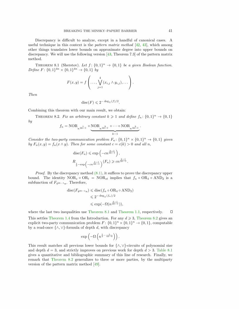
BREAKING THE MINSKY–PAPERT BARRIER 41
Discrepancy is difficult to analyze, except in a handful of canonical cases. Auseful technique in this context is the pattern matrix method [42, 43], which amongother things translates lower bounds on approximate degree into upper bounds ondiscrepancy. We will use the following version [43, Theorem 7.3] of the pattern matrixmethod.
Theorem 8.1 (Sherstov). Let f : 0, 1n → 0, 1 be a given Boolean function.Define F : 0, 14n × 0, 14n → 0, 1 by
F (x, y) = f
. . . , 4∨j=1
(xi,j ∧ yi,j), . . .
.
Then
disc(F ) 6 2− deg±(f)/2.
Combining this theorem with our main result, we obtain:
Theorem 8.2. Fix an arbitrary constant k > 1 and define fn : 0, 1n → 0, 1by
fn = NORn
12k−1
NORn
22k−1
· · · NORn
22k−1︸ ︷︷ ︸
k−1
.
Consider the two-party communication problem Fn : 0, 1n × 0, 1n → 0, 1 givenby Fn(x, y) = fn(x ∧ y). Then for some constant c = c(k) > 0 and all n,
disc(Fn) 6 exp(−cn
k−12k−1
),
R12−exp
(−cn
k−12k−1
)(Fn) > cnk−12k−1 .
Proof. By the discrepancy method (8.1), it suffices to prove the discrepancy upperbound. The identity NORs ORt = NORst implies that fn OR4 AND2 is asubfunction of F42k−1n. Therefore,
disc(F42k−1n) 6 disc(fn OR4 AND2)
6 2− deg±(fn)/2
6 exp(−Ω(nk−12k−1 )),
where the last two inequalities use Theorem 8.1 and Theorem 1.1, respectively.
This settles Theorem 1.4 from the Introduction. For any d > 3, Theorem 8.2 gives anexplicit two-party communication problem F : 0, 1n×0, 1n → 0, 1, computableby a read-once ∧,∨-formula of depth d, with discrepancy
exp(−Ω
(n
12−
14d−6
)).
This result matches all previous lower bounds for ∧,∨-circuits of polynomial sizeand depth d = 3, and strictly improves on previous work for depth d > 3. Table 8.1gives a quantitative and bibliographic summary of this line of research. Finally, weremark that Theorem 8.2 generalizes to three or more parties, by the multipartyversion of the pattern matrix method [49].
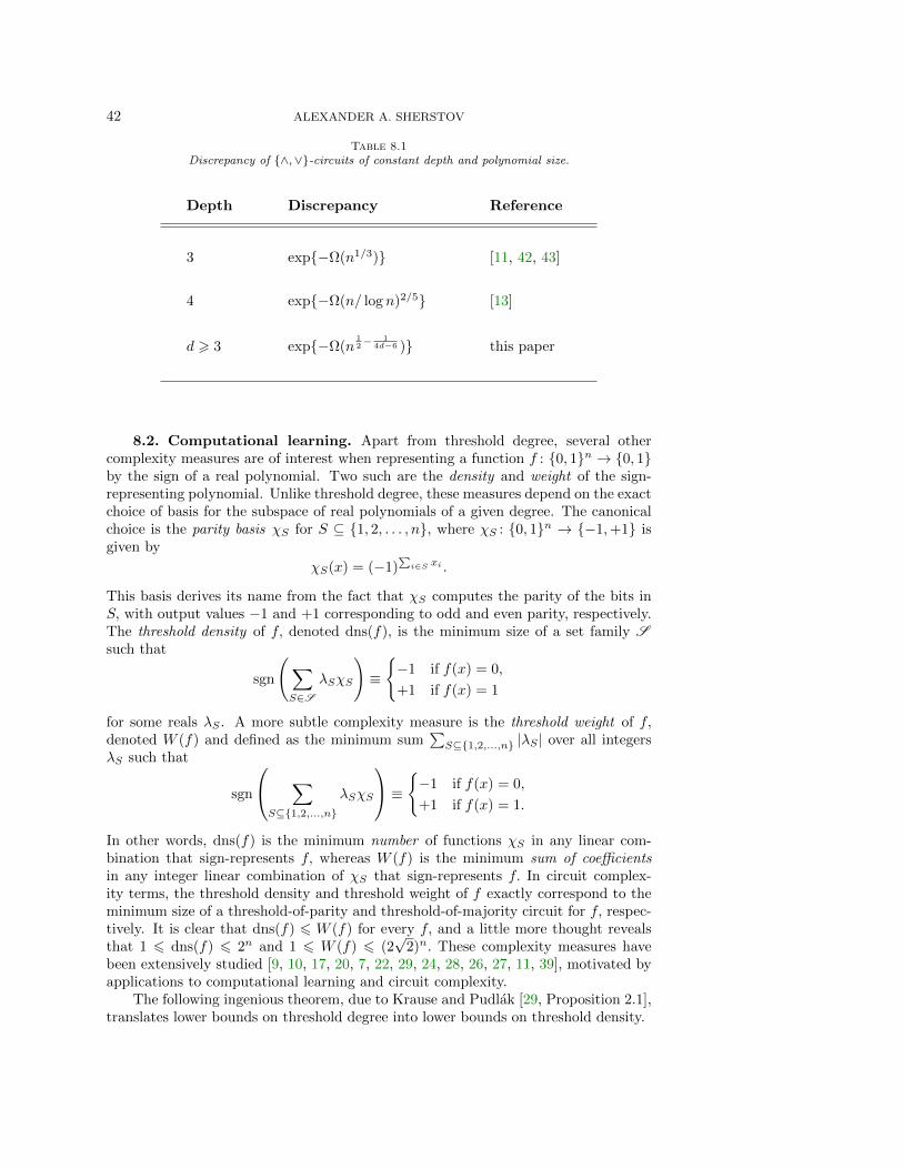
42 ALEXANDER A. SHERSTOV
Table 8.1Discrepancy of ∧,∨-circuits of constant depth and polynomial size.
Depth Discrepancy Reference
3 exp−Ω(n1/3) [11, 42, 43]
4 exp−Ω(n/ log n)2/5 [13]
d > 3 exp−Ω(n12−
14d−6 ) this paper
8.2. Computational learning. Apart from threshold degree, several othercomplexity measures are of interest when representing a function f : 0, 1n → 0, 1by the sign of a real polynomial. Two such are the density and weight of the sign-representing polynomial. Unlike threshold degree, these measures depend on the exactchoice of basis for the subspace of real polynomials of a given degree. The canonicalchoice is the parity basis χS for S ⊆ 1, 2, . . . , n, where χS : 0, 1n → −1,+1 isgiven by
χS(x) = (−1)∑i∈S xi .
This basis derives its name from the fact that χS computes the parity of the bits inS, with output values −1 and +1 corresponding to odd and even parity, respectively.The threshold density of f, denoted dns(f), is the minimum size of a set family Ssuch that
sgn
(∑S∈S
λSχS
)≡
−1 if f(x) = 0,
+1 if f(x) = 1
for some reals λS . A more subtle complexity measure is the threshold weight of f,denoted W (f) and defined as the minimum sum
∑S⊆1,2,...,n |λS | over all integers
λS such that
sgn
∑S⊆1,2,...,n
λSχS
≡ −1 if f(x) = 0,
+1 if f(x) = 1.
In other words, dns(f) is the minimum number of functions χS in any linear com-bination that sign-represents f, whereas W (f) is the minimum sum of coefficientsin any integer linear combination of χS that sign-represents f. In circuit complex-ity terms, the threshold density and threshold weight of f exactly correspond to theminimum size of a threshold-of-parity and threshold-of-majority circuit for f, respec-tively. It is clear that dns(f) 6 W (f) for every f, and a little more thought revealsthat 1 6 dns(f) 6 2n and 1 6 W (f) 6 (2
√2)n. These complexity measures have
been extensively studied [9, 10, 17, 20, 7, 22, 29, 24, 28, 26, 27, 11, 39], motivated byapplications to computational learning and circuit complexity.
The following ingenious theorem, due to Krause and Pudlak [29, Proposition 2.1],translates lower bounds on threshold degree into lower bounds on threshold density.
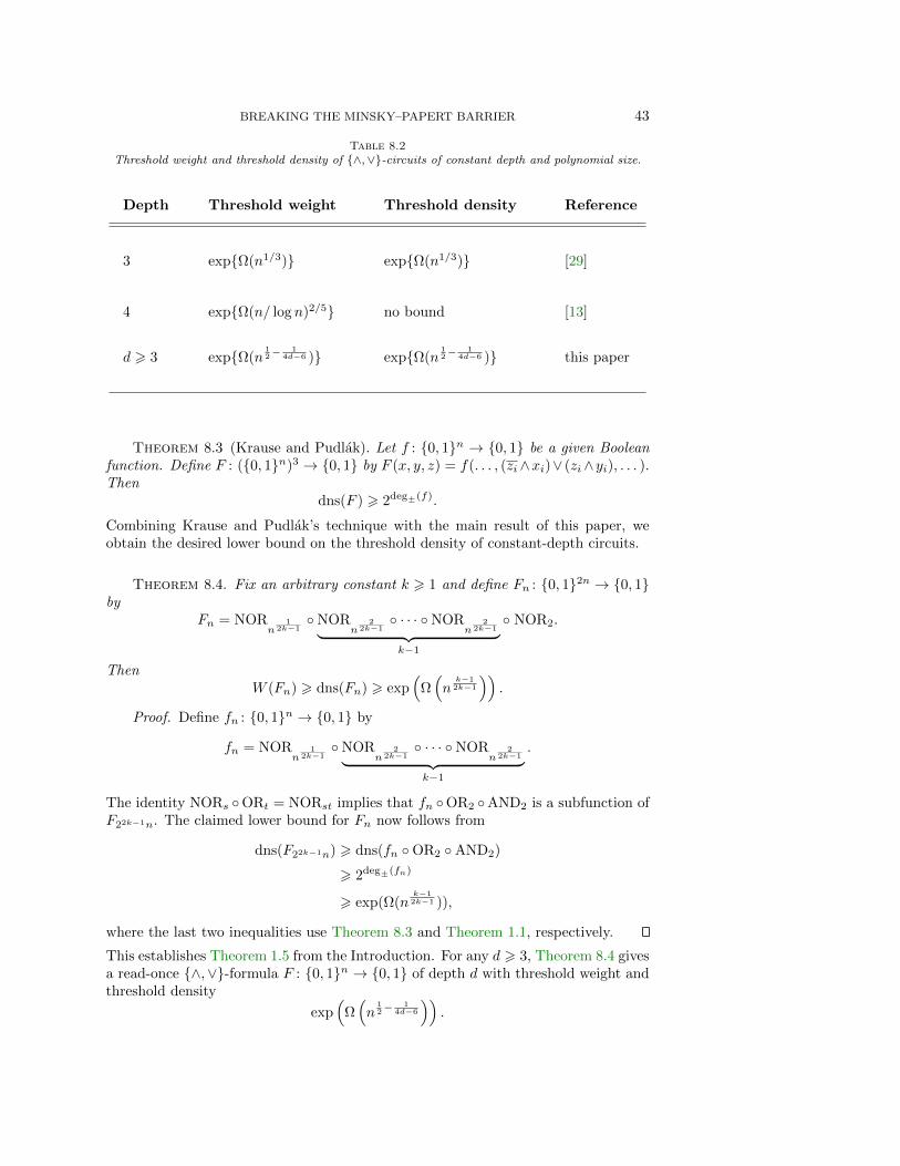
BREAKING THE MINSKY–PAPERT BARRIER 43
Table 8.2Threshold weight and threshold density of ∧,∨-circuits of constant depth and polynomial size.
Depth Threshold weight Threshold density Reference
3 expΩ(n1/3) expΩ(n1/3) [29]
4 expΩ(n/ log n)2/5 no bound [13]
d > 3 expΩ(n12−
14d−6 ) expΩ(n
12−
14d−6 ) this paper
Theorem 8.3 (Krause and Pudlak). Let f : 0, 1n → 0, 1 be a given Booleanfunction. Define F : (0, 1n)3 → 0, 1 by F (x, y, z) = f(. . . , (zi∧xi)∨ (zi∧yi), . . . ).Then
dns(F ) > 2deg±(f).
Combining Krause and Pudlak’s technique with the main result of this paper, weobtain the desired lower bound on the threshold density of constant-depth circuits.
Theorem 8.4. Fix an arbitrary constant k > 1 and define Fn : 0, 12n → 0, 1by
Fn = NORn
12k−1
NORn
22k−1
· · · NORn
22k−1︸ ︷︷ ︸
k−1
NOR2.
ThenW (Fn) > dns(Fn) > exp
(Ω(nk−12k−1
)).
Proof. Define fn : 0, 1n → 0, 1 by
fn = NORn
12k−1
NORn
22k−1
· · · NORn
22k−1︸ ︷︷ ︸
k−1
.
The identity NORs ORt = NORst implies that fn OR2 AND2 is a subfunction ofF22k−1n. The claimed lower bound for Fn now follows from
dns(F22k−1n) > dns(fn OR2 AND2)
> 2deg±(fn)
> exp(Ω(nk−12k−1 )),
where the last two inequalities use Theorem 8.3 and Theorem 1.1, respectively.
This establishes Theorem 1.5 from the Introduction. For any d > 3, Theorem 8.4 givesa read-once ∧,∨-formula F : 0, 1n → 0, 1 of depth d with threshold weight andthreshold density
exp(
Ω(n
12−
14d−6
)).
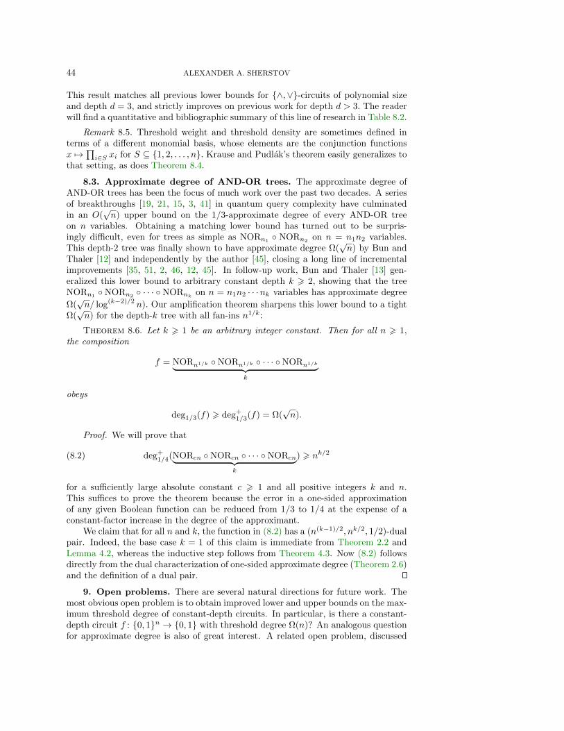
44 ALEXANDER A. SHERSTOV
This result matches all previous lower bounds for ∧,∨-circuits of polynomial sizeand depth d = 3, and strictly improves on previous work for depth d > 3. The readerwill find a quantitative and bibliographic summary of this line of research in Table 8.2.
Remark 8.5. Threshold weight and threshold density are sometimes defined interms of a different monomial basis, whose elements are the conjunction functionsx 7→
∏i∈S xi for S ⊆ 1, 2, . . . , n. Krause and Pudlak’s theorem easily generalizes to
that setting, as does Theorem 8.4.
8.3. Approximate degree of AND-OR trees. The approximate degree ofAND-OR trees has been the focus of much work over the past two decades. A seriesof breakthroughs [19, 21, 15, 3, 41] in quantum query complexity have culminatedin an O(
√n) upper bound on the 1/3-approximate degree of every AND-OR tree
on n variables. Obtaining a matching lower bound has turned out to be surpris-ingly difficult, even for trees as simple as NORn1
NORn2on n = n1n2 variables.
This depth-2 tree was finally shown to have approximate degree Ω(√n) by Bun and
Thaler [12] and independently by the author [45], closing a long line of incrementalimprovements [35, 51, 2, 46, 12, 45]. In follow-up work, Bun and Thaler [13] gen-eralized this lower bound to arbitrary constant depth k > 2, showing that the treeNORn1
NORn2 · · · NORnk on n = n1n2 · · ·nk variables has approximate degree
Ω(√n/ log(k−2)/2 n). Our amplification theorem sharpens this lower bound to a tight
Ω(√n) for the depth-k tree with all fan-ins n1/k:
Theorem 8.6. Let k > 1 be an arbitrary integer constant. Then for all n > 1,the composition
f = NORn1/k NORn1/k · · · NORn1/k︸ ︷︷ ︸k
obeys
deg1/3(f) > deg+1/3(f) = Ω(
√n).
Proof. We will prove that
deg+1/4(NORcn NORcn · · · NORcn︸ ︷︷ ︸
k
) > nk/2(8.2)
for a sufficiently large absolute constant c > 1 and all positive integers k and n.This suffices to prove the theorem because the error in a one-sided approximationof any given Boolean function can be reduced from 1/3 to 1/4 at the expense of aconstant-factor increase in the degree of the approximant.
We claim that for all n and k, the function in (8.2) has a (n(k−1)/2, nk/2, 1/2)-dualpair. Indeed, the base case k = 1 of this claim is immediate from Theorem 2.2 andLemma 4.2, whereas the inductive step follows from Theorem 4.3. Now (8.2) followsdirectly from the dual characterization of one-sided approximate degree (Theorem 2.6)and the definition of a dual pair.
9. Open problems. There are several natural directions for future work. Themost obvious open problem is to obtain improved lower and upper bounds on the max-imum threshold degree of constant-depth circuits. In particular, is there a constant-depth circuit f : 0, 1n → 0, 1 with threshold degree Ω(n)? An analogous questionfor approximate degree is also of great interest. A related open problem, discussed
BREAKING THE MINSKY–PAPERT BARRIER 45
in the previous section, concerns the approximate degree of arbitrary AND-OR treeson n variables. As of this writing, matching lower and upper bounds are knownonly for AND-OR trees of constant depth. Finally, it is a fascinating open prob-lem to determine whether approximate degree is multiplicative in the sense thatdeg1/3(f g) = Θ(deg1/3(f) deg1/3(g)) for all Boolean functions f, g : 0, 1n → 0, 1.Currently, only the upper bound is known to hold (Corollary 2.11).
Appendix A. Constructing a dual object for NOR. The purpose of thisappendix is to prove Theorem 2.9, which gives a dual object for the NOR functionwith a number of additional properties. The development here closely follows earlierwork by Spalek [54] and Bun and Thaler [12]. The main points of departure are amore careful choice of roots for the dual object and the use of shifts, to induce thedesired sign behavior and metric properties. We start with a well-known binomialidentity [18].
Fact A.1. For every polynomial p of degree less than n,
n∑t=0
(−1)t(n
t
)p(t) = 0.
The next lemma constructs a dual object for NOR that has the sign behavior claimedin Theorem 2.9 but may lack the corresponding metric properties.
Lemma A.2. Let ε be given, 0 < ε < 1. Then for some δ = δ(ε) > 0 and everyn > 2, there exists an (explicitly given) function ω : 0, 1, 2, . . . , n → R such that
ω(0) >1− ε
2· ‖ω‖1,(A.1)
(−1)n+tω(t) > 0 (t = 1, 2, . . . , n),(A.2)
deg p <√δn =⇒ 〈ω, p〉 = 0.(A.3)
Proof. We first consider the case of n odd. Let m = 2d4/εe+1 and d = b√n/mc.
Define S = 2 ∪ i2m : i = 0, 1, 2, . . . , d, so that S ⊆ 0, 1, 2, . . . , n. Consider thefunction ω : 0, 1, 2, . . . , n → R given by
ω(t) =(−1)n+t+|S|+1
n!
(n
t
) ∏i=0,1,2,...,n:
i/∈S
(t− i).
Fact A.1 implies that ω is orthogonal to every polynomial of degree at most d, so that(A.3) holds with
δ =1
2d4/εe+ 1.
A routine calculation reveals that
ω(t) =
(−1)|i∈S:i<t|
∏i∈S\t
1
|t− i|if t ∈ S,
0 otherwise.
(A.4)
In particular,
ω(0)
|ω(2)|=
d∏i=1
i2m− 2
i2m> 1−
d∑i=1
2
i2m> 1− 2
m
∞∑i=1
1
i2= 1− π2
3m
46 ALEXANDER A. SHERSTOV
and
ω(0)
|ω(i2m)|=i2m− 2
4· (d− i)! (d+ i)!
d! d!>i2m− 2
4(i = 1, 2, . . . , d).
Hence,
‖ω‖1ω(0)
= 1 +|ω(2)|ω(0)
+
d∑i=1
|ω(i2m)|ω(0)
6 2 +π2
3m− π2+
d∑i=1
4
i2m− 2
6 2 +π2
3m− π2+
4
m− 2
∞∑i=1
1
i2
= 2 +π2
3m− π2+
2
m− 2· π
2
3
6 2 + 2ε,
where the last step holds because m > 8/ε. Now (A.1) is immediate.It remains to examine the sign behavior of ω. Since ω vanishes outside S, the
requirement (A.2) holds trivially at those points. For t ∈ S, it follows from (A.4) that
sgnω(2) = −1,
sgnω(i2m) = (−1)i+1 (i = 1, 2, . . . , d).
Since m is odd, these equations yield sgnω(t) = (−1)t+1 for positive t ∈ S. This settles(A.2) and completes the proof for n odd. The proof for n even is closely analogous,with the difference that one works with the set S = 0 ∪ i2m + 1 : i = 0, 1, 2, . . . for an odd integer m = Θ(1/ε).
We have reached the main result of this section, stated earlier as Theorem 2.9.
Theorem A.3. Let ε be given, 0 < ε < 1. Then for some δ = δ(ε) > 0 and everyn > 2, there exists an (explicitly given) function ω : 0, 1, 2, . . . , n → R such that
ω(0) >1− ε
2· ‖ω‖1,(A.5)
(−1)n+tω(t) >ε
4t2· ‖ω‖1 (t = 1, 2, . . . , n),(A.6)
deg p <√δn =⇒ 〈ω, p〉 = 0.(A.7)
Proof. The cases n = 2 and n = 3 can be handled directly by taking δ = δ(ε) =1/4 and defining
ω : (0, 1, 2) 7→(
1
2− ε
3,−1
2,ε
3
),
ω : (0, 1, 2, 3) 7→(
1
2− ε
3,ε
4,−1
2,ε
12
),
respectively. In the rest of the proof, we treat the complementary case n > 4.
BREAKING THE MINSKY–PAPERT BARRIER 47
For some δ = δ(ε) > 0 and all n > 4, Lemma A.2 ensures the existence of functionsω0 : 0, 1, 2, . . . , 2bn/4c → R and ω1 : 0, 1, 2, . . . , n → R such that
‖ω0‖1 = ‖ω1‖1 = 1,(A.8)
ω0(0) >6− ε
12,(A.9)
ω1(0) >6− ε
12,(A.10)
(−1)tω0(t) > 0, t > 0,(A.11)
(−1)n+tω1(t) > 0, t > 1,(A.12)
deg p <√δn =⇒ 〈ω0, p〉 = 〈ω1, p〉 = 0.(A.13)
For convenience, extend ω0 and ω1 to all of Z by defining these functions to be zerooutside their original domain. Define ω : 0, 1, 2, . . . , n → R by
ω(t) = ω1(t) + ρ
bn/2c∑i=1
(−1)i+n
i2ω0(t− i) + ρ
n∑i=bn/2c+1
(−1)i+n
i2ω0(−t+ i),
where
ρ =5ε
π2(1− ε).
We proceed to verify the three properties of ω claimed in the theorem statement.To begin with,
‖ω‖1 6 ‖ω1‖1 + ρ
n∑i=1
1
i2‖ω0‖1 6 1 + ρ
∞∑i=1
1
i2= 1 + ρ · π
2
6
=6− ε
6(1− ε),(A.14)
where the second inequality uses (A.8). Now (A.5) is immediate because ω(0) =ω1(0) > (6− ε)/12 by (A.10).
Property (A.6) for t > 1 can be verified as follows:
(−1)n+tω(t) = |ω1(t)|+ ρ
bn/2c∑i=1
|ω0(t− i)|i2
+ ρ
n∑i=bn/2c+1
|ω0(−t+ i)|i2
> ρ · |ω0(0)|t2
>5ε
π2(1− ε)· 6− ε
12t2
>ε
4t2· ‖ω‖1,
where the first step follows from (A.11) and (A.12), the third from (A.9), and thefourth from (A.14).
The remaining property (A.7) is immediate from (A.13).
Acknowledgments. The author is thankful to Mark Bun, Ryan O’Donnell,Rocco Servedio, Justin Thaler, and the anonymous reviewers for their valuable feed-back on an earlier version of this manuscript.
48 ALEXANDER A. SHERSTOV
REFERENCES
[1] S. Aaronson and Y. Shi, Quantum lower bounds for the collision and the element distinctnessproblems, J. ACM, 51 (2004), pp. 595–605, doi:10.1145/1008731.1008735.
[2] A. Ambainis, Polynomial degree and lower bounds in quantum complexity: Collision andelement distinctness with small range, Theory of Computing, 1 (2005), pp. 37–46,doi:10.4086/toc.2005.v001a003.
[3] A. Ambainis, A. M. Childs, B. Reichardt, R. Spalek, and S. Zhang, Any AND-OR formulaof size N can be evaluated in time N1/2+o(1) on a quantum computer, SIAM J. Comput.,39 (2010), pp. 2513–2530, doi:10.1137/080712167.
[4] J. Aspnes, R. Beigel, M. L. Furst, and S. Rudich, The expressive power of voting polyno-mials, Combinatorica, 14 (1994), pp. 135–148, doi:10.1007/BF01215346.
[5] L. Babai, P. Frankl, and J. Simon, Complexity classes in communication complexity the-ory, in Proceedings of the Twenty-Seventh Annual IEEE Symposium on Foundations ofComputer Science (FOCS), 1986, pp. 337–347, doi:10.1109/SFCS.1986.15.
[6] P. Beame and T. Huynh, Multiparty communication complexity and threshold circuit size ofAC0, SIAM J. Comput., 41 (2012), pp. 484–518, doi:10.1137/100792779.
[7] R. Beigel, Perceptrons, PP, and the polynomial hierarchy, Computational Complexity, 4(1994), pp. 339–349, doi:10.1007/BF01263422.
[8] R. Beigel, N. Reingold, and D. A. Spielman, PP is closed under intersection, J. Comput.Syst. Sci., 50 (1995), pp. 191–202, doi:10.1006/jcss.1995.1017.
[9] J. Bruck, Harmonic analysis of polynomial threshold functions, SIAM J. Discrete Math., 3(1990), pp. 168–177, doi:10.1137/0403015.
[10] J. Bruck and R. Smolensky, Polynomial threshold functions, AC0 functions, and spectralnorms, SIAM J. Comput., 21 (1992), pp. 33–42, doi:10.1137/0221003.
[11] H. Buhrman, N. K. Vereshchagin, and R. de Wolf, On computation and communicationwith small bias, in Proceedings of the Twenty-Second Annual IEEE Conference on Com-putational Complexity (CCC), 2007, pp. 24–32, doi:10.1109/CCC.2007.18.
[12] M. Bun and J. Thaler, Dual lower bounds for approximate degree and Markov–Bernsteininequalities, Inf. Comput., 243 (2015), pp. 2–25, doi:10.1016/j.ic.2014.12.003.
[13] M. Bun and J. Thaler, Hardness amplification and the approximate degree of constant-depthcircuits, in Proceedings of the Forty-Second International Colloquium on Automata, Lan-guages and Programming (ICALP), 2015, pp. 268–280, doi:10.1007/978-3-662-47672-7 22.
[14] A. Chattopadhyay and A. Ada, Multiparty communication complexity of disjointness, inElectronic Colloquium on Computational Complexity (ECCC), January 2008. ReportTR08-002.
[15] E. Farhi, J. Goldstone, and S. Gutmann, A quantum algorithm for the Hamiltonian NANDtree, Theory of Computing, 4 (2008), pp. 169–190, doi:10.4086/toc.2008.v004a008.
[16] D. Gavinsky and A. A. Sherstov, A separation of NP and coNP in multiparty communicationcomplexity, Theory of Computing, 6 (2010), pp. 227–245, doi:10.4086/toc.2010.v006a010.
[17] M. Goldmann, J. Hastad, and A. A. Razborov, Majority gates vs. general weighted thresholdgates, Computational Complexity, 2 (1992), pp. 277–300, doi:10.1007/BF01200426.
[18] R. L. Graham, D. E. Knuth, and O. Patashnik, Concrete Mathematics: A Foundation forComputer Science, Addison-Wesley, 2nd ed., 1994.
[19] L. K. Grover, A fast quantum mechanical algorithm for database search, in Proceedings ofthe Twenty-Eighth Annual ACM Symposium on Theory of Computing (STOC), 1996,pp. 212–219, doi:10.1145/237814.237866.
[20] J. Hastad, On the size of weights for threshold gates, SIAM J. Discret. Math., 7 (1994),pp. 484–492, doi:10.1137/S0895480192235878.
[21] P. Høyer, M. Mosca, and R. de Wolf, Quantum search on bounded-error inputs, in Proceed-ings of the Thirtieth International Colloquium on Automata, Languages and Programming(ICALP), 2003, pp. 291–299, doi:10.1007/3-540-45061-0 25.
[22] J. C. Jackson, An efficient membership-query algorithm for learning DNF with re-spect to the uniform distribution, J. Comput. Syst. Sci., 55 (1997), pp. 414–440,doi:10.1006/jcss.1997.1533.
[23] M. J. Kearns and U. V. Vazirani, An Introduction to Computational Learning Theory, MITPress, Cambridge, 1994.
[24] A. R. Klivans, R. O’Donnell, and R. A. Servedio, Learning intersections and thresholds ofhalfspaces, J. Comput. Syst. Sci., 68 (2004), pp. 808–840, doi:10.1016/j.jcss.2003.11.002.
[25] A. R. Klivans and R. A. Servedio, Learning DNF in time 2O(n1/3), J. Comput. Syst. Sci.,68 (2004), pp. 303–318, doi:10.1016/j.jcss.2003.07.007.
[26] A. R. Klivans and R. A. Servedio, Toward attribute efficient learning of decision lists and
BREAKING THE MINSKY–PAPERT BARRIER 49
parities, J. Machine Learning Research, 7 (2006), pp. 587–602.[27] A. R. Klivans and A. A. Sherstov, Unconditional lower bounds for learning intersections
of halfspaces, Machine Learning, 69 (2007), pp. 97–114, doi:10.1007/s10994-007-5010-1.Preliminary version in Proceedings of the Nineteenth Annual Conference on ComputationalLearning Theory (COLT), 2006.
[28] M. Krause, On the computational power of Boolean decision lists, Computational Complexity,14 (2006), pp. 362–375, doi:10.1007/s00037-005-0203-0.
[29] M. Krause and P. Pudlak, On the computational power of depth-2 circuits with thresh-old and modulo gates, Theor. Comput. Sci., 174 (1997), pp. 137–156, doi:10.1016/S0304-3975(96)00019-9.
[30] M. Krause and P. Pudlak, Computing Boolean functions by polynomials and threshold cir-cuits, Comput. Complex., 7 (1998), pp. 346–370, doi:10.1007/s000370050015.
[31] E. Kushilevitz and N. Nisan, Communication complexity, Cambridge University Press, 1997.[32] T. Lee, A note on the sign degree of formulas, 2009. Available at http://arxiv.org/abs/0909.
4607.[33] T. Lee and A. Shraibman, Disjointness is hard in the multiparty number-on-the-forehead
model, Computational Complexity, 18 (2009), pp. 309–336, doi:10.1007/s00037-009-0276-2.
[34] M. L. Minsky and S. A. Papert, Perceptrons: An Introduction to Computational Geometry,MIT Press, Cambridge, Mass., 1969.
[35] N. Nisan and M. Szegedy, On the degree of Boolean functions as real polynomials, Compu-tational Complexity, 4 (1994), pp. 301–313, doi:10.1007/BF01263419.
[36] R. O’Donnell and R. A. Servedio, New degree bounds for polynomial threshold functions,Combinatorica, 30 (2010), pp. 327–358, doi:10.1007/s00493-010-2173-3.
[37] R. Paturi and M. E. Saks, Approximating threshold circuits by rational functions, Inf. Com-put., 112 (1994), pp. 257–272, doi:10.1006/inco.1994.1059.
[38] V. V. Podolskii, Perceptrons of large weight, in Proceedings of the Second InternationalComputer Science Symposium in Russia (CSR), 2007, pp. 328–336, doi:10.1007/978-3-540-74510-5 33.
[39] V. V. Podolskii, A uniform lower bound on weights of perceptrons, in Proceedings of theThird International Computer Science Symposium in Russia (CSR), 2008, pp. 261–272,doi:10.1007/978-3-540-79709-8 27.
[40] A. A. Razborov and A. A. Sherstov, The sign-rank of AC0, SIAM J. Comput., 39 (2010),pp. 1833–1855, doi:10.1137/080744037. Preliminary version in Proceedings of the Forty-Ninth Annual IEEE Symposium on Foundations of Computer Science (FOCS), 2008.
[41] B. Reichardt, Reflections for quantum query algorithms, in Proceedings of the Twenty-SecondAnnual ACM-SIAM Symposium on Discrete Algorithms (SODA), 2011, pp. 560–569,doi:10.1137/1.9781611973082.44.
[42] A. A. Sherstov, Separating AC0 from depth-2 majority circuits, SIAM J. Comput., 38 (2009),pp. 2113–2129, doi:10.1137/08071421X. Preliminary version in Proceedings of the Thirty-Ninth Annual ACM Symposium on Theory of Computing (STOC), 2007.
[43] A. A. Sherstov, The pattern matrix method, SIAM J. Comput., 40 (2011), pp. 1969–2000,doi:10.1137/080733644. Preliminary version in Proceedings of the Fortieth Annual ACMSymposium on Theory of Computing (STOC), 2008.
[44] A. A. Sherstov, Strong direct product theorems for quantum communication and query com-plexity, SIAM J. Comput., 41 (2012), pp. 1122–1165, doi:10.1137/110842661. Preliminaryversion in Proceedings of the Forty-Third Annual ACM Symposium on Theory of Comput-ing (STOC), 2011.
[45] A. A. Sherstov, Approximating the AND-OR tree, Theory of Computing, 9 (2013), pp. 653–663, doi:10.4086/toc.2013.v009a020.
[46] A. A. Sherstov, The intersection of two halfspaces has high threshold degree, SIAM J. Com-put., 42 (2013), pp. 2329–2374, doi:10.1137/100785260. Preliminary version in Proceedingsof the Fiftieth Annual IEEE Symposium on Foundations of Computer Science (FOCS),2009.
[47] A. A. Sherstov, Making polynomials robust to noise, Theory of Computing, 9 (2013), pp. 593–615, doi:10.4086/toc.2013.v009a018. Preliminary version in Proceedings of the Forty-FourthAnnual ACM Symposium on Theory of Computing (STOC), 2012.
[48] A. A. Sherstov, Optimal bounds for sign-representing the intersection of two halfspaces bypolynomials, Combinatorica, 33 (2013), pp. 73–96, doi:10.1007/s00493-013-2759-7. Prelim-inary version in Proceedings of the Forty-Second Annual ACM Symposium on Theory ofComputing (STOC), 2010.
[49] A. A. Sherstov, Communication lower bounds using directional derivatives, J. ACM, 61
50 ALEXANDER A. SHERSTOV
(2014), pp. 1–71, doi:10.1145/2629334. Preliminary version in Proceedings of the Forty-Fifth Annual ACM Symposium on Theory of Computing (STOC), 2013.
[50] A. A. Sherstov, The multiparty communication complexity of set disjointness, SIAM J. Com-put., 45 (2016), pp. 1450–1489, doi:10.1137/120891587. Preliminary version in Proceedingsof the Forty-Fourth Annual ACM Symposium on Theory of Computing (STOC), 2009.
[51] Y. Shi, Approximating linear restrictions of Boolean functions. Manuscript, 2002.[52] Y. Shi and Y. Zhu, Quantum communication complexity of block-composed functions, Quan-
tum Information & Computation, 9 (2009), pp. 444–460.[53] K.-Y. Siu, V. P. Roychowdhury, and T. Kailath, Rational approximation techniques for
analysis of neural networks, IEEE Transactions on Information Theory, 40 (1994), pp. 455–466, doi:10.1109/18.312168.
[54] R. Spalek, A dual polynomial for OR. Available at http://arxiv.org/abs/0803.4516, 2008.