breaking the floor of the sf-6d utility function: an ... · de puntuación para el sf-6d, una de...

Documentos de Trabajo5 5 Documentos

de Trabajo2010

José María Abellán PerpiñánFernando I. Sánchez MartínezJorge E. Martínez PérezIldefonso Méndez Martínez

An Application to Spanish Data

Breaking the Floor of the SF-6D Utility Function

Plaza de San Nicolás, 448005 BilbaoEspañaTel.: +34 94 487 52 52Fax: +34 94 424 46 21

Paseo de Recoletos, 1028001 MadridEspañaTel.: +34 91 374 54 00Fax: +34 91 374 85 22

[email protected]

dt_bbva_2010_05_breaking.indd 1 1/7/10 10:33:22



José María Abellán Perpiñán Fernando I. Sánchez Martínez

Jorge E. Martínez Pérez Ildefonso Méndez Martínez

U N I V E R S I T Y O F M U R C I A

Abstract

This working paper presents a new scoring algorithm for the SF-6D, one of the most popular preference-based health status measures. Previous algorithms suffer from a phenomenon called the floor effect (i.e., lack of sensitivity of the instrument for detecting health gains of individuals whose baseline health is poor). Our algorithm expands the range of utility scores in such a way that the floor effect vanishes. We get this wider range thanks to the use of a lottery equivalent method through which preferences are elicited from a representative sample of the Spanish general population.

Key words

SF-36, SF-6D, floor effect, standard gamble, lottery equi-valent methods.

Resumen

Este documento de trabajo presenta un nuevo algoritmo de puntuación para el SF-6D, una de las medidas de salud basadas en preferencias de uso más extendido. Los algo-ritmos previamente estimados adolecen del fenómeno denominado efecto suelo (esto es, la falta de sensibilidad del instrumento para detectar ganancias de salud en indi-viduos cuyo estado de salud de partida es malo). Nuestro algoritmo amplía el rango de utilidades de tal modo que el efecto suelo desaparece. Este rango más amplio se consigue gracias al uso de un método de lotería equiva-lente, con el que se obtienen las preferencias de una muestra representativa de la población española.

Palabras clave

SF-36, SF-6D, efecto suelo, lotería estándar, métodos de lotería equivalente.

Al publicar el presente documento de trabajo, la Fundación BBVA no asu-me responsabilidad alguna sobre su contenido ni sobre la inclusión en el mismo de documentos o información complementaria facilitada por los autores.

The BBVA Foundation’s decision to publish this working paper does not imply any responsibility for its contents, or for the inclusion therein of any supplementary documents or information facilitated by the authors.

La serie Documentos de Trabajo tiene como objetivo la rápida difusión de los resultados del trabajo de investigación entre los especialistas de esa área, para promover así el intercambio de ideas y el debate académico. Cualquier comentario sobre sus contenidos será bien recibido y debe hacerse llegar directamente a los autores, cuyos datos de contacto aparecen en la Nota sobre los autores.

The Working Papers series is intended to disseminate research findings rapidly among specialists in the field concerned, in order to encourage the exchange of ideas and academic debate. Comments on this paper would be welcome and should be sent direct to the authors at the addresses provided in the About the authors section.

Versión: Junio 2010 © los autores, 2010 © de esta edición / of this edition: Fundación BBVA, 2010

EDITA / PUBLISHED BY Fundación BBVA, 2010 Plaza de San Nicolás, 4. 48005 Bilbao

La serie Documentos de Trabajo, así como información sobre otras publicaciones de la Fundación BBVA, pueden consultarse en: http://www.fbbva.es

The Working Papers series, as well as information on other BBVA Foundation publications, can be found at: http://www.fbbva.es

Documento de Trabajo – Núm. 5/2010

3

1. Introduction

THE Short Form 36 (SF-36) is one of the most widely used generic health-related quality of

life measures. It is extensively applied in clinical trials and population health surveys in or-

der to assess changes of health status. Unfortunately, the SF-36 cannot be directly used in

economic evaluations (Brazier et al., 1999) because it does not produce a preference-based

single index able to be combined with life duration in order to obtain quality adjusted life

years (QALYs), the metric used in cost-utility analysis.

The bridging of the gap between the descriptive information provided by the SF-36

and the population’s preferences is provided by algorithms which convert either item res-

ponses, or summary scores, from the SF-36 into utility scores. Pickard et al. (2005) com-

pared ten of such algorithms, most of them based on subsets of items from the SF-36 (e.g.,

the SF-12), concluding that “Brazier's algorithms for the SF-12 and SF-36 appear to be most

favourable because of their methodological and theoretical basis” (p. 8). To estimate such

preference-based algorithms Brazier and colleagues used a subset of SF-36 items, which

were grouped in a six-dimensional measure called the SF-6D (Brazier et al., 1998; Brazier et

al., 2002; Brazier and Roberts, 2004).

Pickard et al. (2005) give three main reasons why the SF-6D is preferable to other

algorithms. First, the SF-6D is based on direct preference measurement. Second, the statisti-

cal design of the study from which preferences were elicited allowed the researchers to ob-

tain a proper representation of severe states. Finally, direct preference measurements were

performed by using the standard gamble (SG), a method which has been usually regarded as

the ‘gold standard’, since it is a choice-based procedure rooted in the axioms of expected

utility theory (Torrance et al., 2001).

Despite all these apparent advantages, it is widely recognized that the SF-6D suffers

from a problem known as the floor effect, that is, the potential lack of sensitivity of the ins-

trument for detecting health gains of individuals whose baseline health is poor (Baker at al.,

1997). Such a potential insensitivity to change has been extensively analyzed in comparison

to the EQ-5D, in such a way that most of the published studies show greater utility benefits

according to the EQ-5D than the SF-6D (Barton et al., 2008). Thus, in general, it could be


4

expected that cost-utility ratios tend to be likely more favourable to the adoption of new

technology according to the EQ-5D rather than with the SF-6D (Pickard et al., 2005). Notice

that we are not asserting that the EQ-5D is a better instrument than the SF-6D, but the floor-

phenomenon, the same as the ceiling effect in the EQ-5D (Brazier et al., 2004), is a factor

that contributes to the disagreement between both preference-based algorithms, enlarging

heterogeneity in cost-utility ratios (Stiggelbout, 2006).

In this paper we argue that, at least partly, the floor effect is caused by the type of

valuation method (the SG) which the SF-6D algorithm is based on. Hence, the last of the

apparent advantages attributed by Pickard et al. (2005) to the SF-6D would be actually a

shortcoming of the model. Our claim is based in that the SG usually gives utility scores

which are too high, suggesting a degree of risk aversion (i.e., a preference for riskless out-

comes) so strong that they cannot be properly described by expected utility. Evidence on the

extreme risk aversion raised by the SG includes studies performed with both monetary out-

comes (Hershey and Schoemaker, 1985; Johnson and Schkade, 1989; Delquié, 1993) and

health outcomes (Wakker and Deneffe, 1995; Bleichrodt et al., 2001; Bleichrodt et al.,

2007).

That the SG yields utilities that are too high for severe health states is fully consis-

tent with the range of scores generated by the SF-6D algorithm (Brazier and Roberts., 2004),

whose lowest value is well above zero (0.296), while the utility score for the worst EQ-5D

health state, according to the TTO tariff for the UK, is -0.594 (Dolan, 1997). Such a large

discrepancy at the lower end of the scale makes the SF-6D gives values higher than those for

the EQ-5D for poorer states, leading in consequence to smaller utility gains for less healthy

people, which is the prediction of the floor effect. Tsuchiya et al. (2006) provide empirical

support to the hypothesis of the relevance of the valuation method in order to explain the

discrepancy between the SF-6D and the EQ-5D, concluding that such a discrepancy is

caused, among other factors, because “the TTO used for EQ-5D (generates) lower scores

than the SG used for more severe SF-6D and higher scores for mild states” (p. 345). Ob-

viously, we are aware that there are other explanations to the floor effect besides the valua-

tion method, such as the apparent inability of the SF-36 items used in the SF-6D to describe

accurately severe health states (Hollingworth et al., 2002). This topic is left aside in this pa-


5

per. Instead, we directly focus on the issue concerning how the validity of the valuation

method behind the SF-6D algorithm can be improved.

This paper reports the results of the first study conducted in Spain to estimate a SF-

6D algorithm for the SF-36. The main novelty of such an algorithm is that it is not based on

the SG. We used instead a variant of the so-called lottery equivalent procedures introduced

by McCord and De Neufville (1986). Such procedures are based on the comparison of two

gambles, and were developed precisely to avoid the dislike for gambling exhibited by me-

thods such as the SG. The psychological intuition for justifying the use of lottery equivalent

methods instead of the SG is that people value outcomes more highly when they occur with

certainty than when they appear in a risky prospect. This phenomenon, commonly referred to

as the certainty effect (Kahneman and Tversky, 1979), makes people facing a SG question

tend to overvalue the riskless outcome in comparison to the gamble, in such a way that the

probability used to yield indifference must be additionally high to compensate for such an

overvaluation of the certainty (Wakker and Stiggelbout, 1995). Such overweighting of the

certainty is “drastically reduced” (Cohen and Jaffray, 1988) when assessments are made by

lottery equivalent methods in which no sure outcome is involved (McCord and de Neufville,

1986; Wakker and Deneffe, 1996; Pinto and Abellan, 2005). This seems to be the main rea-

son why violations of expected utility are less pronounced when both alternatives are risky

(Camerer, 1992). An elaborate theory to justify the use of lottery equivalent methods is pro-

vided by Bleichrodt and Schmidt’s (2002) context-dependent model. In this model expected

utility is satisfied as long as the set of options contains only risky prospects. If the context of

valuation changes, including some riskless outcome, then violations of expected utility are

permitted. Bleichrodt et al. (2007) in a recent study with health outcomes, did not find si-

gnificant differences between two lottery equivalent methods under expected utility, con-

cluding that their data “seem to add to the evidence that violations of expected utility prima-

rily occur when one of the prospects under evaluation is riskless” (p. 479). Nevertheless,

Bleichrodt and Schmidt’s model was not able to reconcile the utilities elicited by such lottery

equivalent methods with the utilities elicited by other three riskless-risk methods (e.g., with

the SG). Probably such a paradox suggests that reality is too complex as to be explained by

one single theory, although, as we have shown, empirical available evidence points out that

one should expect that the floor effect was mitigated by using a lottery equivalent method.


6

The results presented in this paper confirm such a prior expectation: there is not a perceptible

floor effect in the Spanish SF-6D algorithm.

The paper is organized as follows. Section 2 provides background on the SF-6D

classification system and the existing SF-6D algorithms. Section 3 describes the computer

assisted questionnaire we used to survey a sample of the Spanish general population,

outli-ning the differences between our lottery equivalent method and the variant of the SG

used by Brazier and colleagues. Results are described in section 4. Section 5 discusses our

main findings.

2. Background

THE SF-6D (Brazier et al., 2002) takes 11 items from the SF-36 to generate a health status

classification system able to describe a total of 18,000 possible health states. The SF-6D

system has six dimensions (physical functioning, role limitations, social functioning, pain,

mental health, and vitality), each with between four to six levels. Each SF-6D health state is

defined by selecting one level from each dimension. For example, health state 645655 de-

notes the worst possible health state that can be described by the SF-6D system because each

dimension is fixed at its lowest level. For that reason, such a state is called the ‘all worst’ or

‘pits’ health state.

Because of the descriptive richness of the SF-6D system, it is impossible to value all

possible permutations of each dimension. Hence, a subset of health states has to be identified

in order to estimate additive or multiplicative algorithms. Brazier et al. (2002) elicited pre-

ferences for a selection of 249 health states from a sample (N=611) of the UK general popu-

lation. Another recent paper (Lam et al., 2008) reports the results of a pilot survey (N=126)

performed in Hong Kong using the same protocol as in the UK, though only 49 health states

were valued in this case. Such a selection of 49 states, which were already included within

the set valued previously by Brazier et al., result from an orthogonal design which allows the

researchers to estimate an additive model. Brazier et al. included more health states in order

to account for more complex specifications.


7

Bearing in mind that it is impossible that each respondent values the whole selection

of health states, two strategies arise: either maximize the number of health states valued by

each interviewee or, alternatively, maximize the number of respondents who value the same

health state. Both Brazier et al. (2002) and Lam et al. (2008) opted for the first approach, in

such a way that each participant in Brazier et al.’s study valued six SF-6D health states (five

intermediate states plus the ‘pits’ state 645655), whereas respondents surveyed by Lam et al.

valued one state more. This design meant that each health state was valued an average of 15

times.

The elicitation procedure applied in the two abovementioned studies was a chained

SG method. Chained variants for the SG have been proposed (Torrance, 1986) as a way to

avoid that people refuse to accept any risk of death as a typical (unchained) SG question

requires. Such insensitivity at the upper end of the scale was found in Brazier et al.’s (1998)

pilot study, the reason for which Brazier and colleagues decided to valued SF-6D health

states through a two-stage process. In a first stage, Brazier et al.’s (2002) replaced the worst

outcome in a normal SG question (i.e., death) by the ‘pits’ state 645655. Five intermediate

SF-6D health states were valued in such a way. Next, in a second stage, the ‘pits’ state was

valued against death by means of another SG question. The final utility of each intermediate

state was chained to death by means of the ‘pits’ state, allowing the calculation of utilities

onto a scale 0-1 (death-full health). Raw negative utilities for the ‘pits’ state were rescaled in

such a way (Patrick et al., 1994) that the utilities had a lower bound at -1. Indifferences in all

the SG questions were reached by through a sequence of choices implemented in a ‘ping

pong’ way.

The last step to obtain the SF-6D algorithm is the estimation of the model. Ordinary

least squares (OLS) and random effects (RE) models were estimated by Brazier et al. (2002)

to predict all 18,000 SF-6D health states. The model recommended by the authors for use in

cost-utility analysis was an OLS model using mean health state values. Brazier et al. (2004)

improved the previous model by removing non-significant estimates and aggregating those

coefficients which were inconsistent between them. They referred to such a model as the

“parsimonious consistent model”. The econometric methods applied by Lam et al. (2008) to

estimate their algorithm for the Chinese population living in Hong Kong were identical to

Brazier et al.’s (2002).


8

In contrast to previous algorithms, which relied on parametric models, Kharroubi et

al. (2007) -using the same data set as Brazier and colleagues- estimated a set of non-

parametric (Bayesian) utility scores for the SF-6D. Notice that, as the next section will show,

the assumptions behind our estimations are parametric, so our estimates cannot be directly

compared to those inferred by Kharroubi et al. Nevertheless, as far as Kahrroubi et al.’s

(2007) algorithm is affected by the floor effect, the implications derived from using a diffe-

rent valuation method are also applicable to their model.

3. The Valuation Study

3.1. General design

We designed two valuation surveys. The main survey (survey 1) was addressed to

estimate the SF-6D algorithm. This survey included the questions with the lottery equivalent

method. Through the other survey (survey 2) we elicited preferences from an independent

sample in order to test whether the typical (unchained) SG indeed yielded higher utility

scores than our (also unchained) lottery equivalent method. In this way, we tried to corrobo-

rate that the SG produces utilities which are too high, even though there is no chaining in-

volved. There is extensive evidence showing that the chained SG method tends to generate

higher valuations than the unchained one (Llewellyn-Thomas et al., 1982; Rutten-van

Molken et al., 1995; Bleichrodt, 2001; Oliver 2003). Although evidence is much scarcer for

other methods, it appears that chaining leads to higher values as well (Pinto and Abellan,

2005), even affecting (though more weakly) a variant of lottery equivalent methods (Oliver,

2005). In addition to that, chaining is prone to propagation of error (Wakker and Deneffe,

1996).


9

3.2. The sample

We used two independent samples in order to avoid anchor biases and response error

derived from fatigue and cognitive overload. Both samples were representative of the Spa-

nish adult general population with respect to age and sex. As the two samples were randomly

drawn, we expected that preferences in both groups would be similar to each other as long as

a common elicitation procedure was applied. Such an ex-ante homogeneity condition was

tested by including a visual analogue scale (VAS) in the questionnaires administered to both

samples.

The main sample (survey 1) consisted of 1020 subjects. This sample was divided

into 17 subsamples (N=60 each) retaining representativeness with respect to age and sex.

The size of the other sample (survey 2) was identical (N=60) to any of the subsamples used

in survey 1. Both surveys took place in the region of Murcia over a period of two months.

All the interviews were face-to-face and run on laptops. The average time per interview was

around 20 minutes.

3.3. The health states

To select the subset of health states to be directly valued by the respondents we

opted for an intermediate approach between the two extremes represented by Brazier et al.

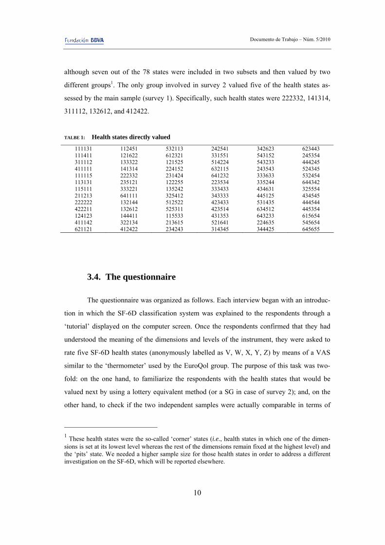
(2002) and Lam et al. (2008). A total of 78 health states (see table 1) were chosen. 49 out of

them were obtained by running the orthoplan module of SPPS version 17. The remaining

states till 78 were selected through a stratified sampling method, and including the ‘pits’

state. Limiting the number of health states directly valued to 78 allowed us to obtain a num-

ber of valuations by state substantially higher (60 valuations per health state on average) than

those obtained previously (15 per health state on average), thus resulting in more liable and

robust mean values. This is of particular relevance since the predictive validity of the estima-

tion methods we applied relies largely on the liability of the sample means. Each of the 17

groups of respondents included in survey 1 valued a different subset of five health states,


10

although seven out of the 78 states were included in two subsets and then valued by two

different groups1. The only group involved in survey 2 valued five of the health states as-

sessed by the main sample (survey 1). Specifically, such health states were 222332, 141314,

311112, 132612, and 412422.

TALBE 1: Health states directly valued

111131 111411 311112 411111 111115 113131 115111 211213 222222 422211 124123 411142 621121

112451 121622 133322 141314 222332 235121 333221 641111 132144 132612 144411 322134 412422

532113 612321 121525 224152 231424 122255 135242 325412 512522 525311 115533 213615 234243

242541 331551 514224 632115 641232 223534 333433 343333 423433 423514 431353 521641 314345

342623 543152 543233 243543 333633 335244 434631 445125 531435 634512 643233 224635 344425

623443 245354 444245 524345 532454 644342 325554 434545 444544 445354 615654 545654 645655

3.4. The questionnaire

The questionnaire was organized as follows. Each interview began with an introduc-

tion in which the SF-6D classification system was explained to the respondents through a

‘tutorial’ displayed on the computer screen. Once the respondents confirmed that they had

understood the meaning of the dimensions and levels of the instrument, they were asked to

rate five SF-6D health states (anonymously labelled as V, W, X, Y, Z) by means of a VAS

similar to the ‘thermometer’ used by the EuroQol group. The purpose of this task was two-

fold: on the one hand, to familiarize the respondents with the health states that would be

valued next by using a lottery equivalent method (or a SG in case of survey 2); and, on the

other hand, to check if the two independent samples were actually comparable in terms of

1 These health states were the so-called ‘corner’ states (i.e., health states in which one of the dimen-sions is set at its lowest level whereas the rest of the dimensions remain fixed at the highest level) and the ‘pits’ state. We needed a higher sample size for those health states in order to address a different investigation on the SF-6D, which will be reported elsewhere.


11

preferences. In the final part of the questionnaire respondents were asked to answer some

sociodemographic questions (sex, age, studies, income level, etc.), to describe their health

status by means of the EQ-5D system, and to complete the items included in the SF-36 (v.2)

health survey.

3.5. Elicitation procedures

3.5.1. The probability lottery equivalent method

The type of lottery equivalent procedure we administered in survey 1 could be called

a probability lottery equivalent (PLE) method since the equivalence between the two gam-

bles is reached by varying the probability of one of them. Notwithstanding, the framing of

such a PLE method is different to those previously used with health outcomes (Oliver, 2005;

Bleichrodt et al., 2007) in one important respect. Our method asks for the probability p that

makes the respondents indifferent between the gamble denoted by (full health, p; death),

yielding full health with probability p and death with probability 1-p, and the 50/50 gamble

denoted by (full health, 0.5; h), yielding full health and the health state h with the same prob-

ability.

This framing allowed us to elicit preferences for both better-than-death and worse-

than-death states, something that, to the best of our knowledge, has never been done before

by using a risky elicitation method. If the respondent preferred the second gamble to the first

one for p = 0.5, it meant that h was regarded as better than death. In consequence, the final

probability of indifference p* was elicited between 0.5 and 1. On the contrary, if the first

gamble was preferred to the second one for p = 0.5, then h was considered as worse than

death, and p* was elicited between 0 and 0.5. Lastly, if the respondent was indifferent be-

tween (full health, 0.5; death) and (full health, 0.5; h), then h was regarded as equal to death.

Under expected utility, assuming the convention that the utility of full health is 1 and the

utility of death is 0, the utility of the health state h is calculated according to the expression

U(h) = 2p* -1.

Our procedure may be intended to be as the analogue under risk to the ‘life profile’

approach developed by Robinson and Spencer (2006) for decisions under certainty for two


12

main reasons. Firstly, the way according to which preferences are elicited is symmetrical for

both better and worse than death health states. That is, irrespective the health state is re-

garded either worse or better than death, the larger the probability p is the milder the health

state is. Secondly, resulting utilities are automatically bounded between -1 and +1 as a con-

sequence that the probability used as stimulus in the assessment of the health state is fixed at

0.5. As it is not obvious why there should be no health states valued below -1 (Devlin et al.,

2008), such possible valuations should not be precluded ex ante, but they should not be

transformed ex post to be bounded by -1 either, which is, unfortunately, the usual practice.

This is the case both the SF-6D (Brazier et al., 2002) and the EQ-5D (Dolan, 1997), whose

rescaled negative utilities are meaningfulness, being no longer possible that they are inter-

preted as true utilities (Patrick et al., 1994). Bearing in mind this, we do not report any indi-

vidual utility reaching -1 in this study2, so no value lower than that bound seems to have

been excluded. We will return to the point of the ability of the PLE to elicit bounded nega-

tive valuations in the Discussion.

In all the questions, the probability of indifference was elicited through a non-

transparent sequence of choices implemented according to the parameter estimation by se-

quential testing (PEST) procedure suggested by Luce (2000). Such a procedure appears to be

less prone to inconsistencies than other search procedures (e.g., ping-pong), in which re-

spondents are aware that the aim of the whole sequence of choices is to produce indifference

(Fischer et al., 1999).

Therefore, the specific lottery equivalent method we applied has, in our opinion, four

potential advantages over the variant of the SG procedure used by Brazier et al. (2002),

namely, that our probability lottery equivalent technique avoids: (i) the certainty effect

caused by the inclusion of a riskless outcome; (ii) the problem of biases and propagation of

error caused by chaining; (iii) the usual methodological drawbacks caused by the valuation

of worse than death health states; and (iv) the potential inconsistencies provoked by using a

transparent sequence of choices to reach indifference.

2 The utilities closest to -1 were five values of -0.96 obtained for the pit state.


13

3.5.2. The standard gamble method

The SG method we used in survey 2 asks the respondents for the probability r that

makes them indifferent between intermediate health state h for sure and a gamble, denoted

by (full health, r; death), yielding full health with probability r and death with probability 1-r.

Under expected utility, assuming the convention that the utility of full health is 1 and the

utility of death is 0, the utility U of the health state h equals r*.

There was no need to apply the variant of the SG able to elicit negative utilities be-

cause none of the respondents regarded any of the five health states as worse than death, so

we omit its description.

3.6. The modelling

Our initial specification is the main effect model which explains the utility score h

that respondent i assigns to health state j using a set of binary dummy variables (xdl) that

describe each level l and dimension d of the health state. For example, x42, denotes dimen-

sion d=4 (pain), level l=2 (there is pain but it does not interfere with normal work). The

model is formally written as follows:

i dl dl id l

h x e

(1)

where ei is a zero-mean error term, and the constant has been forced to unity in order to en-

sure that the health state describing full health has the value of one.

We also estimate more extended versions of equation (1) which include variables

denoting the presence in the state of the highest (worst) level in, at least, one of the dimen-

sions, as well as interactions between variables in the main effect model (e.g., as the so-

called MOST term used by Brazier et al., 2002). The optimal specification is chosen accord-

ing to the usual criteria of consistency (i.e., that utility declines with severity), goodness of


14

fit (i.e., that predictions of the model are accurate), and parsimony (i.e., the simpler the bet-

ter).

When we use individual data, both equation (1) and its extensions are estimated by

the random effect (RE) estimators, that is, assuming that the error term is normally distri-

buted. In particular, we used the RE estimator because it takes into account that the same

individual values several health states, increasing the efficiency of the estimates relative to

an OLS estimator. Thus, the error term e in equation 1 is decomposed into an individual-

specific error term (ηi)3 and a traditional error term unique to each health state and individual

(ij). The coefficients of the model are then identified by estimating equation 1 by maximum

likelihood. The same applies for equations including interaction terms.

Since the model recommended by Brazier et al. (2002) for use in cost-utility analysis

was a model estimated at the mean level, we also estimate mean models. In those cases,

equation 1 and its extensions including interaction terms are estimated by OLS regressions.

4. Results

4.1. The data set

A number of 15 individuals were left out of the analysis because of inconsistencies

in their valuations of health states by means of the VAS and the PLE (survey 1). These in-

consistencies occurred when a logically better health state received a lower value than a

logically worse state. That is the case when a health state that has equal or lower levels than

another state in each of the six dimensions (i.e., it is a milder state) is valued below a health

state with equal or higher levels in each of the six dimensions (i.e., a more severe state).

Another 7 respondents were excluded from the definitive sample because of their reluctance

3 Alternatively, the fixed-effects estimator could be used to correct for individual valuation effects. However, there are efficiency reasons to prefer the RE estimator because the explanatory variables describe a hypothetical health state and, thus, they are uncorrelated to the respondent’s valuation. The results of the Hausman test confirm this reasoning. These results are available upon request to the authors.


15

to assume any risk of death when they answered PLE questions. These 7 individuals were

not willing to assume any risk of death in, at least, three out of the five states that they had to

assess. No exclusion was performed in the sample belonging to survey 2.

TABLE 2: Sociodemographic characteristics of subjects

Sample (n=998) Male/Female (%) 50/50

Mean (SD) age in years 43.6 (16.64)

Marital status Single 33.7 Married/Cohabiting 59.8 Separated/Divorced/Widow 6.5

Education level Illiterate /Primary studies 34.5 Secondary studies 34.4 University studies 31.1

Income level Up to €1,500 22.9 €1,501 – 2,000 28.4 € 2,001 – 3,000 29.8 More than €3,000 18.9

Smoker (%) 27.0

Self-assessed health state (EQ-5D) 11111

60.8

11121 15.8 11112 4.3 Other 19.1

Self-assessed health state (SF-6D/SF-36)) 111122

6.0

111112 4.3 111222 3.1 111111 2.9 Other 83.7

After exclusions, the final sample used as an input to estimate the SF-6D algorithm

consisted of 998 individuals. Table 2 shows sociodemographic characteristics of the sample.

Compared to those of the general population, the study sample was a little younger (nearly

two years and a half) because it was age-stratified (additionally, no subject older than 80

years was selected). Because of the relatively greater youth of our sample, some differences

in educational and income levels arise (our sample has higher levels in both cases). If the

comparison is made with the Spanish population aged between 18 to 75 years, then the mean

age is the same (43.6 years), and differences in terms of education and income largely van-


16

ish. Finally, the sample distribution by sex (male/female) was fairly similar to the general

adult one (50%/50% vs. 49.6%/50.4%).

The information at the end of the table confirms the ‘ceiling effect’ affecting the EQ-

5D system, and the greater sensitivity of the SF-6D to discriminate among mild health states.

Overall, the sensitivity of the SF-6D outperformed that of the EQ-5D, since 80% of the re-

spondents clustered in only three EQ-5D states, while nearly 200 SF-6D states are required

to describe such a percentage of the sample.

4.2. Direct health state valuations

4.2.1. PLE utilities

Some descriptive statistics for a selection of the 78 health states directly valued are

shown in table 3. Each of the states was valued by 64 individuals on average, ranging from a

minimum of 56 subjects to a maximum of 1194. Mean values range from –0.515 to 0.988,

two of the health states showing a negative value. This is in contrast with the results reached

by Brazier et al. (2002), whose mean values were above zero in all cases. Median values

were above mean values for nearly 53% of the health states (41 out of 78), whereas Brazier

et al. reports that their median health state values usually exceeded mean values, reflecting

the positive skewness of their distribution.

At the individual level, our data reveals a certain degree of negative skewness. Al-

though the proportion of utilities below zero is relatively low (4.8%) –even lower than 7%

obtained by Brazier et al. (2002)–, our negative values are, in broad terms, of a larger abso-

lute magnitude than those of Brazier et al. Moreover, one-third of health states (26/78) were

considered worse than death by, at least, one of the respondents. This may help to explain

that our distribution is slightly shifted to the left when compared to that of Brazier et al.

(2002). Mean and median values are lower in our study (0.499 and 0.50 vs. 0.5417 and 0.65,

respectively), and the degree of negative skewness is clearly higher in our data (–1.23 vs.

4 Such a maximum number of respondents was due to the fact that seven health states were valued by two different sub-samples, such as explained in footnote 1.


17

-0.78). Another fact that may help to understand the differences between both studies is that

63% of the respondents in Brazier et al.’s study assigned positive valuations to the ‘pits

state’, whereas a higher percentage (77.5%) of individuals in our study assigned utilities

under –0.30 to the ‘all worst’ health state.

TABLE 3: Statistics for 30 SF-6D health state valuations

State n Min Max Mean Median SD 111411 119 0.540 1.000 0.803 0.780 0.105 112451 60 0.200 0.800 0.515 0.500 0.137 113131 58 0.800 1.000 0.988 1.000 0.036 115111 118 0.300 0.800 0.649 0.660 0.122 121525 60 0.160 0.900 0.569 0.600 0.145 121622 60 0.180 0.700 0.451 0.460 0.103 122255 59 0.200 0.900 0.469 0.460 0.167 132612 59 0.300 1.000 0.710 0.700 0.174 133322 59 0.360 1.000 0.671 0.660 0.136 141314 56 0.240 1.000 0.755 0.800 0.176 222222 60 0.520 1.000 0.891 0.930 0.130 222332 58 0.400 1.000 0.826 0.820 0.136 223534 56 0.060 0.820 0.474 0.420 0.190 224152 60 0.100 0.940 0.411 0.400 0.158 235121 59 0.400 1.000 0.610 0.600 0.134 314345 59 0.200 0.800 0.395 0.400 0.122 325412 58 0.000 0.900 0.552 0.510 0.182 344425 60 0.060 0.580 0.160 0.160 0.085 412422 60 0.300 1.000 0.599 0.600 0.178 434545 59 0.060 0.520 0.241 0.220 0.102 445125 60 0.100 0.800 0.369 0.330 0.140 512522 59 0.200 0.800 0.476 0.500 0.130 524345 59 -0.400 0.700 0.285 0.300 0.142 532454 58 -0.980 0.860 0.161 0.200 0.436 615654 60 -0.960 0.620 -0.263 -0.310 0.346 621121 60 0.240 0.980 0.657 0.700 0.176 634512 56 -0.200 0.600 0.158 0.100 0.172 643233 60 0.060 0.700 0.315 0.300 0.178 644342 57 -0.980 0.660 0.004 0.060 0.366 645655 116 -0.980 0.500 -0.515 -0.600 0.426

To check to what extent the mean health state values were logically consistent, we

examined all the ordinal pairwise comparisons that were possible from the 78 health states.

There are 558 comparisons in which one of the sates should be valued logically higher than

the other one, since the former has equal or lower levels than the latter for each of the six


18

dimensions5. When mean values for these comparable states are confronted, logical inconsis-

tencies only emerge for 2.51% (14/558). The fact that such a low inconsistency rate was

found despite only five health sates being valued by each of the respondents, suggests that it

is possible to assess a broad set of health states without overloading the interviewees, avoid-

ing in this way the rise of random error due to tiredness and boredom.

4.2.2. Comparison between PLE and SG utilities

VAS scores for the five health states valued both in survey 1 and survey 2 were very

similar to each other (p>0.05), in such a way that the result of the comparison between PLE

and SG utilities for the same states could be considered as meaningful even though they

came from two independent samples. Such a result is shown in table 4. It is apparent that

both mean and median utilities measured by means of the SG were significantly higher than

those assessed through the PLE, corroborating our prior expectation of the discrepancy be-

tween the two methods.

TABLE 4: Probability lottery equivalent (PLE) vs. Standard gamble (SG) valuations

Mean valuations Median valuations Health states

PLE SG t-test

(p-value) PLE SG

Wilcoxon (p-value)

222332 0.711 0.815 0.000 0.700 0.800 0.000 141314 0.754 0.846 0.000 0.780 0.850 0.002 311112 0.832 0.905 0.025 0.820 0.900 0.025 132612 0.880 0.955 0.000 0.940 0.950 0.001 412422 0.599 0.780 0.000 0.600 0.800 0.000

5 There are two exceptions to this consistency rule in the SF-6D. Firstly, levels 5/6 of the "physical functioning" dimension ("your health limits you a little/a lot in bathing and dressing") does not neces-sarily imply a poorer condition than that of levels 3/4 ("your health limits you a little/a lot in moderate activities"). In a similar way, level 3 of the "role limitations" dimension ("you accomplish less than you would like as a result of emotional problems") does not reveal a worse health condition than that described in level 2 ("you are limited in the kind of work or other activities as a result of emotional problems").


19

4.3. SF-6D algorithms

Estimated coefficients are shown in table 5 for the three models which led to the best

results in terms of goodness of fit and parsimony. Two of them are RE models at individual

level data, whereas the third one is an OLS model using mean values. The RE model labelled

as the ‘raw model’ is the starting model at individual level data, without removing non-

significant variables. The RE model labelled as the ‘efficient model’ was constructed by

eliminating non-significant regressors from the ‘raw model’ and by grouping the variables of

whichever two consecutive levels when their coefficients are not significantly different from

each other. This procedure maximizes the degrees of freedom available for the model esti-

mation, as well as preventing from certain inconsistencies in predicting the tariff. These

slight inconsistencies may result from differences in the estimation of the coefficients which

correspond to consecutive levels that are not significantly different from each other6. The

mean OLS model is the algorithm more comparable to the “preferred” one by Brazier et al.

(2002), since both are mean level models. Finally, unlike Brazier and colleagues we did not

find any significant interaction term (e.g., the term they called MOST), so all our algorithms

only reflect main effects.

The inspection of table 5 reveals that all the coefficients have the expected sign and

are highly significant, with only the exemption of the coefficient corresponding to level 2 of

the ‘role limitation’ dimension in the ‘raw’ RE model. There is an apparent inconsistency in

both RE models between coefficients PF4 and PF5 in such a way that the coefficient asso-

ciated to level 5 is lower in absolute value than the coefficient associated to level 4. How-

ever, as it was noted before (footnote 4) such an apparent inconsistency is not real, since

those levels are not logically comparable. Thus, all our models are actually consistent.

6 Brazier et al. (2002) group together the coefficients of whichever two consecutive levels when the estimated coefficient for the lower level is of a higher absolute value, that is to say, when the tariffs yielded by the estimated model are inconsistent. Our model is consistent, so our concern is its effi-ciency.


20

Moreover, the mean absolute error (MAE) attached to any of our models is only slightly

higher than that reported by Brazier et al. (2002), who used a substantially higher number of

health states, which shows the quality of fit we obtained.

TABLE 5: SF-6D(SF-36) health state models

Random effects models OLS mean model

‘Raw’ (1)

Efficient (2)

Mean (3)

Cons 1 Cons 1 Cons 1 PF2 -0,025 PF2 -0,022 PF2 -0,015 PF3 -0,056 PF3 -0,062 PF3 -0,034 PF4 -0,120 PF4 -0,122 PF4 -0,090 PF5 -0,107 PF5 -0,109 PF5 -0,111 PF6 -0,335 PF6 -0,340 PF6 -0,338 RL2 0,007 RL2 -0,014 RL3 -0,045 RL23 -0,018 RL3 -0,038 RL4 -0,089 RL4 -0,085 RL4 -0,070 SF2 -0,071 SF2 -0,069 SF2 -0,037 SF3 -0,078 SF3 -0,079 SF3 -0,060 SF4 -0,194 SF4 -0,194 SF4 -0,203 SF5 -0,239 SF5 -0,234 SF5 -0,208 PAIN2 -0,044 PAIN2 -0,018 PAIN3 -0,047 PAIN23 -0,044 PAIN3 -0,034 PAIN4 -0,172 PAIN4 -0,178 PAIN4 -0,198 PAIN5 -0,230 PAIN5 -0,225 PAIN5 -0,202 PAIN6 -0,343 PAIN6 -0,345 PAIN6 -0,318 MH2 -0,026 MH2 -0,029 MH2 -0,066 MH3 -0,050 MH3 -0,053 MH3 -0,078 MH4 -0,072 MH4 -0,075 MH4 -0,096 MH5 -0,196 MH5 -0,199 MH5 -0,224 VIT2 -0,043 VIT2 -0,042 VIT2 -0,058 VIT3 -0,093 VIT3 -0,091 VIT3 -0,121 VIT4 -0,158 VIT4 -0,156 VIT4 -0,157 VIT5 -0,181 VIT5 -0,179 VIT5 -0,199

n 4.990 n 4.990 n 78

Predictive ability

MAE 0.0871 0.0872 0.0812 | pred. Error | < k k = 0,01 8.13 4.72 11.72 k = 0,05 36.41 35.25 36.49 k = 0,10 63.50 62.24 70.50

Note: All coefficients are significant at a 99% confidence level except for PF2 in models (1) and (2), and RL(3) in model (2), which are signifi-cant at the 95% level; and RL2 in model (1) which is statistically non-significant. The estimation of the mean model incorporates corrective weights to account for the fact that mean health state values are not always calculated using the same number of observations.


21

The values of the coefficients for the two RE models suggest that the greater utility

loss associated to the maximum level of severity in a dimension occurs for ‘Pain’, ‘Physical

functioning’ and ‘Social functioning’ attributes, in this order. The conclusion, however, dif-

fers slightly for the OLS model at mean level, since it is ‘Physical functioning’ the dimen-

sion that produces the larger disutility, followed by ‘Pain’ and ‘Social functioning’.

The OLS Mean model in column 3 is somewhat superior to RE models in terms of

predictive ability. Although its MAE is only marginally lower, the distribution of prediction

errors is slightly better than in RE ‘raw’ and efficient models. In consequence, the estimation at

mean level is chosen as the preferred one. Since Brazier et al. (2002) and Brazier and Roberts

(2004) also chose their mean OLS models among all other estimations, then the comparison of

our results with those of Brazier and colleagues can be done in homogeneous terms.

Figure 1 shows the distribution of predicted utilities by both our mean OLS model

and Brazier and Roberts (2004) mean consistent model. It is apparent that our model ‘breaks’

the minimum threshold of Brazier and Roberts’s algorithm, expanding the left tail of the

distribution near and even below zero. The minimum score predicted by our mean model is

-0.357, a value very far from 0.296, the minimum threshold predicted by the UK tariff. We

can conclude then that the Spanish SF-6D algorithm presented in this paper does not seem to

suffer from the floor effect.

Since the percentage of negative valuations in our study was even lower than those

found by Brazier and colleagues (4.8% vs. 7%), one possible objection to our estimates could be

that they are not consistent once a minimum fraction of observations are removed from the data

set. To explore this possibility we repeated the OLS estimation by excluding from the data suc-

cessively 5%, 10%, and 20% of the individuals with the lowest valuations, and afterwards we

redid the analyses. The predicted utilities derived from the most demanding case (20% of exclu-

sions) are shown in Figure 2. As can be observed, our SF-6D algorithm seem largely robust to

the elimination of extreme values, which suggests that our model is very solid7. The minimum

value of the Spanish tariff displayed in the figure is -0.231.

7 The conclusion is analogue for RE estimations.


22

FIGURE 1: A comparison of the Spanish and UK tariffs’ predicted values 0

12

34

5

-.5 0 .5 1

UK Tariff Spanish Tariff

Note: The Spanish Tariff corresponds to our OLS mean model in Table 5. The UK Tariff is the SF-6D (SF-36) ‘consistent’ model at mean level (column 2 of Table 4 in Brazier and Roberts, 2004).

FIGURE 2: Consistency-analysis. Spanish tariff after excluding 20% of the subjects from the

sample vs. UK tariff

01

23

45

-.5 0 .5 1

UK Tariff Spanish Tariff (20%)


23

5. Discussion

THE main conclusion of this paper is that it is possible to expand the range of SF-6D utility

scores by using a different valuation method. In other words, it is possible to avoid the

‘floor’ effect without changing the SF-6D health status classification system. As we noted in

the introduction we are aware that the SF-6D has problems when describing severe health

states, but even so the sensitivity of the SF-6D algorithm for less healthy people can be

largely improved if it is based on preferences elicited by means of a lottery equivalent

method instead of the standard gamble.

Brazier et al. (2002) recommended their mean model (10) for use in cost-utility an-

alysis. Brazier and Roberts (2004) modified such a model in order to get a consistent algo-

rithm (i.e., an algorithm without coefficients that decrease in absolute size with a worse

level) which became the new preferred specification. If our mean model is compared with

Brazier and Roberts’s consistent model a great discrepancy arises between them. Basically,

the ‘tariff’ that predicts our algorithm is shifted to the left with regards to that predicted by

the consistent model. We have a significant part of the distribution (around one-fourth) be-

low 0.3, which is the minimum threshold of Brazier and Roberts’s algorithm. In fact, the

value predicted by our algorithm for the worst SF-6D health state is far below zero, -0.357.

We checked the robustness of our algorithm by dropping those individuals who gave the

lowest utilities, verifying that the main message of our study remains true: the floor effect is

broken. After removing 20% of the respondents, the minimum value of our mean model is

-0.231, a score clearly below zero.

Our mean model has a predictive ability slightly lower than Brazier and Roberts’s

(2004) (0.081 vs 0.074), but it exhibits a much greater internal consistency, since no incon-

sistency between coefficients on the SF-6D levels appear. We have not had to aggregate

inconsistent estimates in order to achieve a consistent scale, such as Brazier and Roberts had

to do, because all our coefficients were directly consistent. Moreover, all the coefficients in

our mean model were significant, in such a way we did not have to remove any coefficient.

The econometric models we used are the same as Brazier and his colleagues applied

in previous studies, so our findings cannot be justified on such a basis. It is true that none of

our models included the interaction term MOST, but if we compare the range of the SF-6D


24

values predicted by our mean model with that predicted by Brazier et al.’s (2002) main effect

model (6), our range continues to be larger. The same occurs if the comparison is performed

with respect to Lam et al.’s (2008) main effect model. Hence, it appears that it is necessary

to look for other explanations to our findings.

One logical source of differences may come from the fact that our tariff is based on

the Spanish population’s preferences instead of British people’s preferences as was the case

of previous tariffs. It is evident that such a factor may explain a part of the discrepancy be-

tween British and Spanish SF-6D tariffs. We have some indirect evidence to support this

from the comparison between the Spanish EQ-5D tariff and the UK one. Apparently, there

exists genuine differences in preferences between the two countries, in such a way that the

Spanish respondents tend to attach a higher weight to the functional dimensions of mobility,

self-care and usual activities, whereas the UK respondents seem to assign greater weight to

the more symptoms-based dimensions of pain/discomfort and anxiety/depression (Badía et

al., 2001). However, even acknowledging such a variation in preferences between the two

countries, it does not cause a change in the shape of the distribution of EQ-5D scores as dras-

tic as in our case with the algorithm for the SF-6D. Therefore, it seems that country-specific

differences though likely to affect results, cannot explain our findings by themselves.

Another difference with regards to Brazier et al.’s (2002) study is the design of the

survey. Our respondents only had to value five health states, whereas respondents involved

in Brazier et al.’s study valued one state more. Apart from that difference, the interview pro-

tocol used in our study is not the same as that applied by Brazier et al. (2002). Nevertheless,

the design followed by Lam et al. (2008) to estimate the SF-6D algorithm in Hong Kong was

not the same either, and despite this, their results were broadly similar to those obtained for

the UK algorithm. On the other hand, the EQ-5D tariff has been estimated by using very

different designs (e.g., Dolan, 1997 vs Lamers et al., 2006) but the resulting score ranges

have not been so different to each other as occurs in our case.

Therefore, it seems that our findings cannot be successfully explained unless we fo-

cus on the different valuation method used. There are both empirical evidence (Bleichrodt et

al., 2007) and theoretical arguments (Bleichrodt and Schmidt, 2002) to expect that a lottery

equivalent method such as we applied leads to lower scores than those yielded by the stan-

dard gamble. The valuations obtained for 78 SF-6D health sates were congruent with such a


25

prior expectation, in such a way that mean, median and minimum values were lower in our

study than in other studies previously performed. In addition to that, the comparison between

our probability lottery equivalent method and the standard gamble for five different SF-6D

health states confirmed the hypothesis that the standard gamble yields values which are too

high.

We think that the weaknesses of the standard gamble are well established in the lit-

erature. The SG does not only suffer from failures of internal consistency (Bleichrodt, 2001;

Oliver, 2003), but also seems to have a poor external validity, which casts doubts about how

suitable the use of SG-based algorithms is (Abellan-Perpiñan et al., 2009). The potential

drawbacks affecting lottery equivalent methods are much less known, however we are aware

that such procedures may be also affected by biases. For example, the same as probability

weighting may cause an upward bias in SG measurements (Bleichrodt, 2002), it might also

make that utility values elicited by lottery equivalent methods even were too low (Wakker

and Stiggelbout, 1995). Moreover, the specific probability equivalent method used in this

study may not be exempted of potential limitations. As noted previously this procedure is

able to make that utilities are bounded between -1 and +1. This is not a property of the ge-

neric family of lottery equivalent techniques, but a direct consequence of fixing at 0.5 the

probability attached to full health in the lottery serving as stimulus in the elicitation. There is

not lower bound at -1 for any other probability value different from 0.5. This feature of the

PLE prompts questions about if the range of utilities actually measured by such a method

might vary depending on which the ‘baseline’ probability was. This issue deserves to be

explored in future investigations.

Notwithstanding, even taken into account all these possible limitations, given the

substantial body of evidence suggesting that expected utility violations primarily arise for

riskless-risk comparisons, we think that at present the balance is favourable to lottery equiva-

lent methods, including the specific PLE applied in this study. Thus, we are inclined to see

the floor effect as, in part, the result of applying an elicitation method –the SG- prone to bias

utilities upward because of the overvaluation of the certain alternative which is confronted

with the gamble. The PLE is the device we have used to obtain less biased inputs to estimate

the SF-6D algorithm. The practical consequence of this ‘debiasing’ process is that the result-

ing range of SF-6D utilities is now more similar to that generated by the EQ-5D.


26

Further research is needed to explore in depth the validity of our new algorithm. For

example, future investigations might address the task of comparing for the same subjects

probability lottery equivalent measurements with standard gamble assessments adjusted ac-

cording to prospect theory. In this way, we could test if, as Bleichrodt et al. (2007) found,

prospect theory does not affect probability lottery equivalent values, whereas the standard

gamble ones are largely reduced. Another interesting issue would be the development of new

algorithms, using the same data set as this paper, by relaxing the parametric assumptions that

are behind both random effects and OLS models. Finally, comparisons with EQ-5D tariffs

should also be made, in order to obtain direct evidence as to what extent the two instruments,

the SF-6D and the EQ-5D, are more comparable, after the floor effect has vanished.

6. References

ABELLAN-PERPIÑAN, J.M., H. BLEICHRODT and J.L. PINTO-PRADES (2009): “The predictive validity of

prospect theory versus expected utility in health utility measurement”. Journal of Health

Economics 28(6), 1039-1047.

BADIA, X., R. ROSET, M. HERDMAN and P. KIND (2001): “A comparison of GB and Spanish general

population time trade-off values for EQ-5D health states”. Medical Decision Making 21(1),

7-16.

BAKER D.W., R.D. HAYS and R.H. BROOK (1997): “Understanding changes in health status. Is the

floor phenomenon merely the last step of the staircase?”. Medical Care 35, 1-15.

BARTON, G., T. SACH, A. AVERY, C. JENKINSON, M. DOHERTY, D. WHYNES and K. MUIR (2008): “A

comparison of the performance of the EQ-5D and SF-6D for individuals aged ≥ 45 years”.

Health Economics 17, 815-832.

BLEICHRODT, H. (2001): “Probability weighting in choice under risk: an empirical test”. Journal of

Risk and Uncertainty 23, 185-198.

____ (2002): “A new explanation for the difference between time trade-off utilities and standard gam-

ble utilities”. Health Economics 11, 447-456.


27

BLEICHRODT, H., J.M. ABELLAN-PERPIÑAN J.L. PINTO and I. MENDEZ (2007): “Resolving Inconsisten-

cies in Utility Measurement under Risk: Tests of Generalizations of Expected Utility”. Man-

agement Science 53, 469-482.

BLEICHRODT, H., J.L. PINTO and P. WAKKER (2001): “Making descriptive use of prospect theory to

improve the prescriptive use of expected utility”. Management Science 47, 1498-1514.

BLEICHRODT, H., and U. SCHMIDT (2002): “A context-dependent model of the gambling effect”. Man-

agement Science 48, 802-812.

BRAZIER, J., M. DEREVILL, C. GREEN, R. HARPER and A. BOOTH (1999): “A review of the use of

health status measures in economic evaluation”. Health Technology Assessment 3(9).

BRAZIER, J. and J. ROBERTS (2004): “The estimation of a preference-based measure of health from the

SF-12”. Medical Care 42, 851-859.

BRAZIER J., J. ROBERTS and M. DEVERILL (2002): “The estimation of a preference-based measure of

health from the SF-36”. Journal of Health Economics 21: 271-292.

BRAZIER, J., J. ROBERTS, A. TSUCHIYA and J. BUSSCHBACH (2004): “A comparison of the EQ-5D and

SF-6D across sever patients groups”. Health Economics 13, 873-884.

BRAZIER, J., T. USHERWOOD, R. HARPER and K. THOMAS (1998): “Deriving a preference-based single

index from the UK SF-36 health survey”. Journal of Clinical Epidemiology 51, 1115-1128.

CAMERER, C. (1992): “Recent tests of generalizations of expected utility theory”. In W. Edwards, ed.

Utility: Theories, Measurement and Applications. Boston, MA: Kluwer Academic Publish-

ers, 207-251.

COHEN, M. and J. JAFFRAY (1988): “Certainty effect versus probability distortion: an experimental

analysis of decision making under risk”. Journal of Experimental Psychology 14, 554-560.

DEVLIN, N., A. TSUCHIYA, K. BUCKINGHAM and K. TILLING (2009): “A uniform time trade off method

for states better and worse than death: feasibility study of the ‘lead time’ approach”. City

University Economics Discussion Papers No. 09/08. London: Department of Economics,

School of Social Sciences, City University London.

DELQUIÉ, P. (1992): “Inconsistent trade-offs between attributes: new evidence in preference assess-

ment biases”. Management Science 39, 1382-1395.

DOLAN, P. (1997): “Modeling valuations for EuroQol health states”. Medical Care 35(11), 1095-1108.


28

FISCHER, G.W., Z. CARMON, D. ARIELY and G. ZAUBERMAN (1999): “Goal-based Construction of

Preferences: Task Goals and the Prominence Effect”. Management Science 45: 1057-1075.

HERSHEY, J.C. and P.J. SCHOEMAKER (1985): “Probability versus certainty equivalence methods in

utility measurement: Are they equivalent?”. Management Science 31, 1213-1231.

HOLLINGWORTH, W., R.A. DEYO, S.D. SULLIVAN, S.S. EMERSON, D.T. GRAY and J.G. JARVIK (2002):

“The practicality and validity of directly elicited and SF-36 derived health state preferences

in patients with low back pain”. Health Economics 11(1), 71-85.

JOHNSON, E. and D. SCHKADE (1989): “Bias in utility assessments: Further evidence and explana-

tions”. Management Science 35, 406-424

KAHNEMAN, D. and A. TVERSKY (1979): “Prospect theory: An analysis of decision under risk”. Ec-

onometrica 47(2), 263–291.

KHARROUBI, S., J.E. BRAZIER, J.R. ROBERTS and A. O’HAGAN (2007): “Modelling SF-6D health state

preference data using a nonparametric Bayesian method”. Journal of Health Economics

26(3), 597-612.

LAM, C.L., J. BRAZIER and S.M. MCGHEE (2008): “Valuation of the SF-6D health states is feasible,

acceptable, reliable, and valid in a Chinese population”. Value in Health 11, 295–303.

LLEWELLYN-THOMAS, H.A., H.J. SUTHERLAND, R. TIBSHIRANI, A. CIAMPI, J.E. TILL and N.F. BOYD

(1982): “The Measurement of Patients' Values in Medicine”. Medical Decision Making 2,

449-462.

LUCE, R.D. (2000): Utility of Gains and Losses: Measurement-Theoretical and Experimental Ap-

proaches. New Jersey: Lawrence Erlbaum Associates, Inc.

MCCORD, M. and R. DE NEUFVILLE (1986): “Lottery equivalents: Reduction of the certainty effect

problem in utility assessment”. Management Science 32(1), 56-60.

OLIVER, A. (2003): “The internal consistency of the standard gamble: tests after adjusting for prospect

theory”. Journal of Health Economics 22, 659-674.

____ (2005): “Testing the internal consistency of the lottery equivalents method using health out-

comes”. Health Economics 14, 149-159.

PATRICK, D.L., H.E. STARKS, K.C. CAIN, R.F. UHLMANN and RA. PEARLMAN (1994): “Measuring

preferences for health states worse than death”. Medical Decision Making 14, 9-18.


29

PICKARD, S.A., Z. WANG, S.M. WALTON and T.A. LEE (2005): “Are decisions using cost-utility analy-

ses robust to the choice of SF-36/SF-12 preferenced-based algorithm?”. BMC Health Qual.

Life Outcomes 3: 1–9.

PINTO, J.L. and J.M. ABELLÁN-PERPIÑÁN (2005): “Measuring the health of populations: the veil of

ignorant approach”. Health Economics 14, 69–82

ROBINSON, A. and A. SPENCER (2006): “Exploring challenges to TTO utilities: valuing states worse

than dead”. Health Economics 15, 393-402.

RUTTEN-VAN-MÖLKEN, M.P., C.H. BAKKER, E.K.A. VAN DOORSLAER and S. VAN DER LINDEN (1995):

“Methodological issues of patient utility measurement. Experience from two clinical trials”.

Medical Care 33(9), 922-937.

STIGGELBOUT, A. (2006): “Health state classification systems: how comparable are our cost-

effectiveness ratios?”. Medical Decision Making 26, 223-225.

TORRANCE, G.W. (1986): “Measurement of health state utilities for economic appraisal”. Journal of

Health Economics 5, 1–30.

TORRANCE, G.W., D. FEENY and W. FURLONG (2001): “Visual Analog Scales: Do They have a Role in

the Measurement of Preferences for Health States?”. Medical Decision Making 21, 329-334

TSUCHIYA, A., J. BRAZIER and J. ROBERTS (2006): “Comparison of valuation methods used to generate

the EQ-5D and the SF-6D value sets”. Journal of Health Economics 25, 334-346.

WAKKER, P. and A. STIGGELBOUT (1995): “Explaining distorsions in utility elicitation through the

rank-dependent model for risky choices”. Medical Decision Making 15, 180-186.

WAKKER, P. and D. DENEFFE (1996): “Eliciting von Neumann-Morgenstern Utilities when Probabili-

ties are Distorted or Unknown”. Management Science 42(8), 1131-1150.


30

NOTA SOBRE LOS AUTORES - ABOUT THE AUTHORS*

JOSÉ MARÍA ABELLÁN PERPIÑÁN holds a PhD in economics and business from the University of Murcia where he is currently professor of applied economics. His primary research interests include behavioural economics, experimental economics and health economics. He has published several articles in Spanish and international journals, and co-authored several books concerning issues in medical decision making and economic evaluation of health technologies. He is currently involved in several projects addressing the issue of the value of life and health for public policy. E-mail: [email protected] JORGE EDUARDO MARTÍNEZ PÉREZ graduated in economics and holds a PhD in economics from the University of Murcia, where he is currently professor of applied economics. His specialist fields are health economics, value of life and labour economics. He has published various books and articles in Spanish and international journals. E-mail: [email protected] ILDEFONSO MÉNDEZ MARTÍNEZ holds a PhD in economics from CEMFI and is currently professor of applied economics at the University of Murcia. His specialised fields are labour economics, policy evaluation and health economics. He has participated in many Spanish and international congresses and has published in international journals. E-mail: [email protected] FERNANDO IGNACIO SÁNCHEZ MARTÍNEZ holds a PhD in economics and busi-ness from the University of Murcia where he is currently professor of applied economics. His research is focused on health economics and, particularly, on the economic evaluation of health technologies. He has published several papers in Spanish and international journals, as well as some monographs, on these topics. He has also written some papers on fiscal federalism and local public fi-nance. He has joined in several publicly and privately financed research pro-jects. E-mail: [email protected]. ________________________________________________________________

Any comments on the contents of this paper can be addressed to José M.ª Abellán, De-partamento de Economía Aplicada, Facultad de Economía y Empresa, Campus de Espi-nardo, 30100 Murcia, Spain. E-mail: [email protected]. * The authors gratefully acknowledge financial support from the Regional Health Mi-nistry of the Autonomous Community of Murcia.


31

ÚLTIMOS NÚMEROS PUBLICADOS – RECENT PAPERS

DT 04/10 Análisis del potencial socieconómico de municipios rurales con métodos no paramétricos: Aplicación al caso de una zona Leader

Ernest Reig Martínez

DT 03/10 Corpus lingüístico de definiciones de categorías semánticas de personas mayo-res sanas y con la enfermedad de Alzheimer: Una investigación transcultural hispano-argentina

Herminia Peraita Adrados y Lina Grasso

DT 02/10 Financial Crisis, Financial Integration and Economic Growth: The European Case Juan Fernández de Guevara Radoselovics y Joaquín Maudos Villarroya

DT 01/10 A Simple and Efficient (Parametric Conditional) Test for the Pareto Law

Francisco J. Goerlich Gisbert

DT 16/09 The Distance Puzzle Revisited: A New Interpretation Based on Geographic Neutrality

Iván Arribas Fernández, Francisco Pérez García y Emili Tortosa-Ausina

DT 15/09 The Determinants of International Financial Integration Revisited: The Role of Networks and Geographic Neutrality Iván Arribas Fernández, Francisco Pérez García y Emili Tortosa-Ausina

DT 14/09 European Integration and Inequality among Countries: A Lifecycle Income Analysis José Manuel Pastor Monsálvez y Lorenzo Serrano Martínez

DT 13/09 Education, Utilitarianism and Equality of Opportunity Aitor Calo-Blanco y Antonio Villar Notario

DT 12/09 Competing Technologies for Payments: Automated Teller Machines (ATMs), Point of Sale (POS) Terminals and the Demand for Currency Santiago Carbó-Valverde y Francisco Rodríguez-Fernández

DT 11/09 Time, Quality and Growth Francisco Alcalá

DT 10/09 The Economic Impact of Migration: Productivity Analysis for Spain and the United Kingdom Mari Kangasniemi, Matilde Mas Ivars, Catherine Robinson y Lorenzo Serrano Martínez

DT 09/09 Endogenous Financial Intermediation Radim Bohácek y Hugo Rodríguez Mendizábal

DT 08/09 Parameterizing Expectations for Incomplete Markets Economies Francesc Obiols-Homs

Documentos de Trabajo5 5 Documentos

de Trabajo2010

José M.ª Abellán PerpiñánFernando I. Sánchez MartínezJorge E. Martínez PérezIldefonso Méndez Martínez



Plaza de San Nicolás, 448005 BilbaoEspañaTel.: +34 94 487 52 52Fax: +34 94 424 46 21

Paseo de Recoletos, 1028001 MadridEspañaTel.: +34 91 374 54 00Fax: +34 91 374 85 22

[email protected]

dt_bbva_2010_05_breaking.indd 1 23/6/10 16:58:40

breaking the floor of the sf-6d utility function: an ... · de puntuación para el sf-6d, una de...

Documents