Breadwinning Mothers and Children’s Gender Norms

Panos Mavrokonstantis∗

October 9, 2017

Abstract

I study how mothers’ relative (to fathers’) earnings affect children’s attitudes towardsgender roles. Prior literature finds a positive relation between maternal labor supplyand the development of egalitarian gender attitudes. Using data from England, I showthat what matters is not simply whether the mother works, but whether she works andearns more than the father. In doing so, I uncover striking heterogeneity between boysand girls. While boys with breadwinning mothers (i.e. mothers earning more than thefathers) are less likely to develop traditional views, girls in such families are more likely tobecome traditional, in opposition to their family’s norm but in line with society’s. Themain gender role I consider is whether mothers with young children should ever workfull-time, but find the same heterogeneity when examining children’s views along otherdimensions related to gender norms. Specifically, girls with breadwinning mothers arealso less likely to believe that earning high wages is important for them and are less likelyto want to study science at university. I develop a model of gender identity, showing thatmy results can be explained by girls’ weaker preference for conformity to their family. Iuse conformity measures to show that this prediction holds empirically, and implementa regression discontinuity design to estimate the effect of living in such norm-minorityfamilies on conformity.

Keywords: gender norms, gender inequality, regression discontinuityJEL codes: D10, J16, Z13

∗Department of Economics, London School of Economics, 32 Lincoln’s Inn Fields, London, WC2A 3PH,UK, p.mavrokonstantis@lse.ac.uk. I thank Sebastian Camarero-Garcia, Sarah Clifford, Frank Cowell, AndersJensen, Alan Manning, Arthur Seibold, Viktorie Sevcenko, Johannes Spinnewijn, and seminar participants atthe LSE, LBS, EPRU Copenhagen, ECINEQ Luxembourg, ECINEQ Canazei, LAGV Marseille and EALEGhent for helpful comments and discussions. I acknowledge financial support from the Onassis Foundation.All remaining errors are my own.

1

1 IntroductionSignificant attention has been given to the recent rise of female breadwinners in the UK (IPPR2015). The proportion of mothers earning more than 50% of the family’s income has doubledbetween 1997-2014, increasing from 10% to 20%1. The increase in this nontraditional familystructure is challenging the age-old traditional model of the male breadwinner and femalecaregiver. An unexplored question is whether this recent phenomenon, currently driven bya minority of the population, can change the norms about the appropriate roles of men andwomen in society.

In this paper, I examine the extent to which gender norms are passed on from one gen-eration to the next when a family’s norms oppose those of the society in which the familyis embedded. Do children growing up in nontraditional families (i.e. where the mother isthe breadwinner) adopt their family’s values or those of society? Using data from England,I find unusual results for girls. While boys raised in nontraditional families are less likelyto develop traditional norms, girls raised in nontraditional families are actually more likelyto do so, in opposition to their family’s norm but in line with society’s. Examining furtheroutcomes associated with gender norms, I also find that girls raised in nontraditional familiesare less likely to state that being able to earn high wages is important for them and are lesslikely to want to study science at university. Employing a model of gender identity to ex-amine the gender-socialization process, I argue that my results can be explained by a weakerpreference among girls for conforming to the family. I then use empirical conformity measuresto show that the theoretical predictions do indeed hold in the data. Specifically, I find thatgirls in nontraditional families are less likely to have chosen their studies based on what theirparents wished, and are more likely to argue with them. Finally, I examine the mechanismdriving this heterogeneity in conformity. Using quasi-experimental variation and a regressiondiscontinuity design, I show that this weaker preference is caused by the treatment of living ina nontraditional family, making girls react to their family’s norm-minority status and adoptmore traditional views.

These findings have strong policy implications given that the individual gender attitudesdeveloped by the end of the teenage years are significant determinants of labor supply inadulthood (Johnston et al. 2014). Moreover, the prevailing gender norm of society is a strongpredictor of gender inequality in the labor market. Consider, for instance, Figure 1a, whichshows the relation between the gender pay gap and the prevalence of traditional gender normsacross OECD countries. There is a strong positive relation between the proportion of a coun-try’s population that believes women should not work full-time, and the percentage differencein the median wage between men and women. Similar conclusions can be drawn from Figures1b and 1c. The more traditional a country is, the lower female labor supply is, both alongthe extensive (Figure 1b) and intensive margins (Figure 1c). These stylized facts elucidatehow important gender norms are to the analysis of gender inequality. Understanding theirintergenerational transmission process can help identify policies that promote more egalitar-ian social norms, the benefits of which go beyond reducing labor market inequalities. Moreequal gender norms can aid in removing barriers to human development (UNDP 2014) andmitigate the adverse consequences of gender inequality traps (in particular gender gaps in ed-ucation) on economic development (Dollar and Gatti 1999; Klasen 1999; Knowles et al. 2002;

1Author’s calculations based on the Family Resources Survey.

2

World Bank 2006). The modernization of gender norms and the associated increase in femalelabor-market participation may also act as a key mechanism to fight poverty and promoterural development, measures that the Food and Agriculture Organization (2009) has stronglyadvocated. Indeed, recent work by Kleven and Landais (2017) shows that egalitarian gendernorms are strong predictors of economic development.

This study makes several contributions. First, it adds to a growing body of work exploringpsychological attributes and preferences as drivers of gender inequality. These include riskpreferences, attitudes towards competition or negotiation, and altruism2. This paper adds tothese by exploring a new mechanism: gender socialization and preferences for conformity toexisting gender norms.

Second and most important, this study shows that explicitly defining parents’ gender val-ues, by distinguishing between nontraditional and traditional families, is crucial for assessingwhether intergenerational transmission of gender norms is successful. The main approach inthe literature is to examine the relation between mothers’ and daughters’ labor supply (DelBoca et al. 2000; Fernandez et al. 2004; Morrill and Morrill 2013; Olivetti et al. 2016; etc.).The finding of a positive correlation has been interpreted as evidence that nontraditional gen-der attitudes are successfully transmitted. I argue that this interpretation is problematic.Daughters of mothers who worked may well have a higher likelihood to also work, comparedto daughters of mothers who did not work. However, the daughters of working mothers maystill be working and earning less than their husbands. Hence, what the literature describes asevidence of the transmission of nontraditional values may still be capturing the propagationof traditional, male-breadwinner family norms. I find evidence consistent with this reasoning.I replicate the finding that girls are less likely to develop traditional views if their motherworks. However, I also find that they are more likely to become traditional if their motherworks or earns more than their father. To my knowledge, this is the first study to highlightthis dichotomy by examining the effect of living in a nontraditional versus a traditional familyon gender norms. The only related study is by Bertrand et al. (2015), which does not havean intergenerational approach but examines between-spouse outcomes. My study tries to fillthis gap.

Lastly, in testing the assumptions of my identification strategy I uncover a caveat relatedto the findings of the Bertrand et al. (2015) influential study on the distribution of wives’income shares. In their study on the US, they find a sharp drop in the density of wives’ incomeshares at the 0.5 threshold, which is interpreted as an aversion to the wife earning more thanthe husband. I show that at least in the UK, this phenomenon is purely driven by familieswith earnings from self-employment, who exhibit very significant bunching at the thresholdbeyond which the wife starts to earn more. In families with only wage income however, no suchsorting is found. This non-finding is consistent with significant earnings adjustment frictionshighlighted in recent public finance literature (Chetty et al. 2011; Kleven and Waseem 2013;Gelber et al. 2016).

The paper proceeds as follows. Section 2 reviews the literature. Section 3 describes thetheoretical framework using a model of gender identity, and Section 4 discusses the first empir-ical approach. Section 5 describes the data and presents evidence on the social norm regardinggender roles in England. Section 6 discusses the results, and Section 7 presents a regressiondiscontinuity design to examine the mechanism driving the main findings. Section 8 concludes.

2For a review, see Bertrand (2010).

3

2 Literature ReviewA vast literature in sociology and social psychology exists on theories of socialization andsocial identity (Tajfel 1978; Lytton and Romney 1991; Lorber 1994; Epstein and Ward 2011).The aim of this literature is to explain how individuals develop their understanding aboutwhat behaviors and opinions are considered appropriate by society. The main principle is thatsocialization, i.e. the process of learning about such values through human interaction, is themain way cultural norms are developed, adopted and transmitted.

Although studies on the role of socialization in the intergenerational transmission of cul-tural values exist in the literature of other social sciences, economists have only recently begunto explore the topic. The seminal work bridging this gap between economics and other dis-ciplines is that of Akerlof and Kranton (2000; 2002; 2010), who translated theories of socialidentity into an economics framework, giving birth to what is now known as Identity Eco-nomics. Various approaches to modelling identity have ensued3. Among others, Benabou andTirole (2007) propose a model where individuals hold a range of individual beliefs that theyboth value and can invest in. Klor and Shayo (2010) model identity as status, while Bisinet al. (2011) introduce the concept of oppositional identities. Although the models differ,the common element in this literature is the introduction of identity considerations into aneoclassic framework in which a person’s self-image is valued and becomes a crucial elementof her utility function.

A burgeoning empirical literature has developed that examines the effect of culture andits transmission. However, little work exists on the intergenerational transmission of explicitgender norms. Most studies that do consider gender norms focus rather on the effect of normson some other outcomes (predominantly labor supply), without examining how gender normsare formed in the first place. For instance, Bertrand et al. (2015) examine the effect oftraditional gender norms (defined as aversion to the wife earning more than the husband)on marriage and labor-market outcomes. While they argue that this aversion is inducedby gender-identity norms, they do not assess how these norms are formed or transmittedintergenerationally, but simply take them as given. They show that women are less likely towork if their potential income exceeds their husbands’; if they do work, women are more likelyto earn less than their potential income. Further, such female breadwinner families face ahigher likelihood of divorce and lower marriage satisfaction.

Using a different approach, Alesina and Giuliano (2010) assess family culture by study-ing the importance of family ties for economic behavior. They find that stronger family tiesare associated with lower female labor force participation. Their explanation is that strongfamily ties require an adult family member to stay home and ‘manage’ the family institu-tion, and this burden falls on women, who are consequently excluded from the formal labormarket. In a related paper on culture, Alesina et al. (2013) look at the historical origins ofgender norms. They provide evidence for intergenerational cultural persistence, showing thatattitudes towards women are more traditional among descendants of societies that practisedplough agriculture. Plough agriculture, in contrast to shifting cultivation, was more capitalintensive and therefore required brawn-intensive labor, favouring men and leading to gender-based division of labor. As a result, the authors find historical plough use to be negativelyrelated to modern-day attitudes towards gender inequality, female labor force participation,

3For a comprehensive survey of identity models, see Costa-Font and Cowell (2015).

4

and female participation in politics and firm ownership. In a somewhat different setting, Fer-nandez and Fogli (2009) examine how ancestral culture is related to fertility and labor marketoutcomes of second-generation American women. They find that women work more (havemore children) in cases in which their country of ancestry had higher historic female laborforce participation (total fertility rate).

Another strand of the literature looks at the relation between the labor supply of individualsand that of their parents. The overall findings indicate a positive correlation, implying thatgender norms are transmitted from one generation to the next. For instance, Fernandez et al.(2004) find that women are more likely to work if their mother-in-law also worked, while Morrilland Morrill (2013) show that there is a positive relationship between mothers’ and daughters’labor supply. In line with these findings, Del Boca et al. (2000) also find that women’s laborsupply is related to that of both their mothers and mothers-in-law, while Olivetti et al. (2016)find a positive relation between daughters’ number of hours worked and the hours worked byboth their own mothers and the mothers of their childhood peers.

Other studies move away from labor market outcomes and analyze gender norms by ex-ploring marital satisfaction among males. Butikofer (2013) finds marital satisfaction to belower when a man’s wife works and contributes to household income, but only for men raisedin a traditional family where the mother did not work. Similar findings are reported byBonke (2008) and Bonke and Browning (2009). This result provides evidence that gendersocialization at the family level, and at a young age, is crucial in determining lifelong gendernorms.

The relation between gender norms and educational outcomes has also been studied re-cently. For instance, Gonzales de San Roman and de la Rica Goiricelaya (2012) examine thecross-country gender gap in test scores revealed by PISA data. They find gender norms tobe an important determinant; in particular, mothers’ labor force participation is positivelyrelated to daughters’ test performance. In a different setting, Blunch and Das (2014) showthat increased access to education for girls explains much of the rise in egalitarian views to-wards female access to education in Bangladesh. Similarly, employing data from 157 countries,Cooray and Potrafke (2010) find conservative culture and religion to be the primary obstacletowards gender equality in education.

Last but not least, some papers investigate the relationship between parental and child gen-der attitudes. Both Farre and Vella (2013) and Johnston et al. (2014) find strong correlationsin these attitudes in cases in the USA and UK, respectively. In line with previous findings,these two studies also find a positive association between boys’ attitudes during childhood andtheir future wives’ labor supply in adulthood.

3 The Theoretical FrameworkThis section describes the process through which children develop their beliefs. Socializa-tion is first explained, followed by a simple model that formalizes this process through autility-maximizing framework. Some theoretical predictions follow, which will be useful ininterpreting the empirical results in subsequent sections.

5

3.1 The Socialization Process

Children develop gender norms through socialization (Epstein and Ward 2011; etc.). Socialpsychology identifies two main sources of socialization: the family (vertical socialization) andsociety at large (horizontal socialization). Children acquire norms by interacting with andobserving the particular behaviors of these two social institutions.

The family is, of course, the first point of contact with the outside world. Therefore,parents play a key role in socialization. Parents are assumed to be altruistic towards theirchildren, and have preferences regarding the norms children develop. In particular, they aim tosocialize their children to their own values. Parents choose how much effort to exert to increasethe probability that vertical socialization is successful. Effort in this setting can manifest intwo main ways. The first is that parents can express their beliefs through direct discussionwith their children, which requires investment in ‘family time’. Effort can also take the formof parents’ actions, particularly the role adopted by each parent. Children thereby receivesignals about appropriate gender roles by observing their parents’ household responsibilities,in particular who the breadwinner is and who is responsible for household production andchild care.

As children grow older and start to interact with a social circle beyond their families, theyare also exposed to what society at large deems to be the appropriate role of women. Theprimary sources of horizontal socialization are the child’s school, peer group, and exposure tosocial norms through mass media.

Each child has some preference for conforming to the family and society. This preferencewill depend not only on individual characteristics, but also on the probability that familysocialization was successful. This probability in turn, will depend on family and social norms;families following the social norm will have a higher chance of transmitting their values becausethey will not have to overcome an opposing social norm.

Having learnt what the family and society believe to be the appropriate gender roles, thechild chooses her own gender values. In doing so, the child takes into account the cost ofdeviating from these norms. This can be thought of as a psychological cost of interactingwith others who do not share the same beliefs, and arises from self-image concerns, that is,concerns about how personal views will be judged by others. The stronger the preference forconformity is, the higher is the cost of deviating from the prescribed norms.

3.2 Formalizing the Socialization Process

To formalize this process, I build on the Georgiadis and Manning (2013) model of nationalidentity. In my setting, each child has the following utility function:

U = −1

2

[cF (xF , xS, Z)(x− xF )2 + cS(xF , xS, Z)(x− xS)2

](1)

where:

6

x ∈ [0, 1] represents the child’s choice; higher x indicates more traditional beliefsxF ∈ [0, 1] is the child’s family norm; higher xF indicates more traditional beliefsxS ∈ [0, 1] is society’s norm; higher xS indicates more traditional beliefscF ∈ (0, 1] is how strongly the child wants to conform to the familycS ∈ (0, 1] is how strongly the child wants to conform to the society

Z is a vector of characteristics affecting preferences for conformity

The intuition of the model is simple. The larger the distance between the child’s belief(x) and that of the family’s (xF ) and society’s (xS), the larger the psychological cost is. Thiscost is increasing in the preference for conformity to the family (cF ) and society (cS). Thestronger this preference is, the more costly it is to deviate from a norm to which the childwants to conform. Taking this into account, the child chooses her optimal belief according tothe following rule:

x∗ = argmaxx

U = x(cF , cS, xF,xS, Z) =cF (xF , xS, Z)xF + cS(xF , xS, Z)xScF (xF , xS, Z) + cS(xF , xS, Z)

(2)

Hence, the child chooses how traditional her gender view will be by weighting the familyand social norms by her preferences for conforming to each.

3.3 Comparative Statics

I now use the model to predict how a change in conformity preferences will affect x∗, as thiswill be useful for interpreting my empirical results. The comparative statics are as follows:

∂x∗

∂cF=

cS(xF , xS, Z)(xF − xS)(cF (xF , xS, Z) + cS(xF , xS, Z))

2 (3)

(3) shows the response of x∗ to a stronger preference for conformity to the family4. Itssign depends on which institution is more traditional, society or the family. As I will show inSection 5.1, the social norm in England regarding the role of mothers with young children isvery traditional, while in the empirical framework (Section 4), the family norm I will examinewill represent very nontraditional views. Thus, without loss of generality, these norms can bemodelled by setting xF = 0 and xS = 1. Given these restrictions, the prediction is that astronger preference for conforming to the family’s norm leads to a decrease in x∗, that is toa less traditional norm. The intuition is that the more strongly a child wants to conform toher family’s relatively less traditional norm, the more she has to differentiate herself from thetraditional social norm and adopt a more nontraditional belief. Otherwise, the psychologicalcost of deviating from the less traditional norm, to which she now wants to conform morestrongly, will increase. I revisit this result in Section 7 where I rationalize my finding thatgirls growing up in nontraditional families develop more traditional views5.

4An analogous result holds for the case of preferences for conformity to society.5In Appendix A, I also discuss the prediction ∂x∗

∂xFand show how it matches my empirical results.

7

4 The Empirical FrameworkMy aim is to estimate x∗ = x(xF , xS, Z). The Next Steps survey (described in the next section)provides data on children’s gender norms through responses to the following question: “Womenshould never work full-time when they have young children. Do you agree with this statement? ”Stating that a woman should never work full-time if she has young children reflects a verytraditional view of gender roles; within the language of the model, this implies x∗ = 1. Basedon this, I define the outcome variable capturing children’s norms as follows:

Traditional Norm =

{1 if Agree (x∗ = 1)

0 if Disagree (x∗ < 1)

As the aim is to examine the intergenerational transmission of gender norms, I have toassess how successful vertical and horizontal gender socialization are. Since the children inthe survey are all from England, they are all exposed to the same social norm6. The variationof interest will therefore come from differences in family norms. Because I am particularlyinterested in examining the development of children’s norms when the family and social normare oppositional, I define the family norm in a way that translates into the model as xF = 0.I do so using the following definition:

Nontraditional Family =

{1 if Mother Earns More than Father0 otherwise

I thus want to examine how children’s gender norms develop when living in a nontraditionalfamily but a traditional society (evidence on the English society’s gender norm is shown inSection 5.1). Moreover, I am interested in between-sex heterogeneity in gender socialization.I will therefore estimate the following (linear) probability model7:

Pr(Traditional Norm)i = β0 + β1Nontraditional Familyi + β2Femalei+

β3Nontraditional Familyi × Femalei + Z′

iζ + ui(4)

where Z is a vector of covariates to be controlled for. The identifying assumption here isselection on observables, i.e. E(ui|Nontraditional Familyi, Femalei, Zi) = 0. While this isnot a weak assumption, it is not implausible given the vast array of characteristics that Z willinclude. Nevertheless, Section 7 will present another identification strategy - a regression dis-continuity design - to provide stronger evidence that the findings have a causal interpretation.

6The social norm may of course still vary by region. To account for this, regional fixed effects are includedin all empirical specifications.

7All probability models presented in this paper have also been estimated using probit and logit specifications,with results being very robust. Results are available upon request.

8

5 Data

5.1 The Social Norm

What is the social norm to which the children in my sample are exposed? I answer thisusing information from the International Social Survey Programme (ISSP), which collectsdata internationally on a broad range of social issues. Questions related to gender norms areincluded in the 1988, 1994, 2002, and 2012 surveys. Responses from the 2002 survey werechosen, since this is the period that coincides with the Next Steps survey, with children in thesample aged between 15 and 16 at the time. The ISSP 2002 contains data from a representativesample of 1960 observations from the UK. Because I study views on the appropriate roles ofmen and women in childrearing and in providing income, I focus on heterosexual couples withchildren and analyze the labor supply of both the father and the mother. In particular, I lookat their responses to the following four questions:

“Did you work full-time, part-time, or not at all when. . . ”

1. “. . . you had no children”

2. “. . . you had a child under school age”

3. “. . . your youngest child was still in school”

4. “. . . your children left the home”

These four cases track the parents’ labor market activity from the time before the child isborn (case 1), up to adulthood (case 4). Cases 1 and 4 focus on parents with no dependentchildren. Case 2 concerns parents with children under four years of age, and case 3 focuseson parents of school-age children. Figure 2 shows the responses to each question for both thefathers and mothers. Figure 2a reflects the first case, showing that there is no prescriptionagainst women working full-time when they have no children. When they have no child careresponsibilities, over 80% of women work full-time, and only a small minority stay at home(less than 9%). Compared to the fathers’ labor supply however, the changes in the mothers’labor supply when they have children are striking. Figure 2b reveals that when women havechildren below the age of four, the majority (53%) do not work at all, while the percentangeof those working full-time drops from 82% to 14%. In the same circumstance, the proportionof fathers working full-time remains steadily above 90%. These figures reveal how traditionalthe social norm in the UK is. There is a strong prescription that the role of mothers withyoung children is not at the workplace.

This is evident despite the large opportunity cost of doing so. Note that maternity leavein the UK is not very generous. Mothers enjoy a replacement rate of 90% for just the firstsix weeks, and receive a fixed amount of £100 per week for up to 18 weeks (in the periodstudied)8. Despite the large amount of foregone earnings of mothers staying at home beyond

8In 2002, maternity (job-protected) leave could be taken for up to 39 weeks. Maternity pay could only bereceived for 18 weeks, at a rate of 90% of previous earnings for the first six weeks, and a fixed amount cappedat £100 per week for the remaining period. A 2003 reform increased maternity leave to 52 weeks and pay to26 weeks, but the 90% replacement rate was still paid for only the first six weeks, with the capped amount forthe remainder. Statutory paternity leave did not exist in 2002.

9

the first six weeks9, most women do not work for up to four years after child birth. Thisfurther highlights that the social norm is for the father to work full-time and provide for thefamily, and for the mother to reduce her labor supply in order to provide child care.

This prescription holds for all women who have dependent children. Figure 2c shows thatthe majority of women (nearly 80%) still do not work full-time, even though their childrenare older but still of school age. Working full-time only becomes the mode again when thechildren have grown up and left the home (Figure 2d), although the proportion of women inthis category is still low (46%) compared to the first case. It is also interesting to note howstable men’s labor supply is. While the age of a child strongly predicts the mother’s laborsupply, fathers always work full-time regardless of the presence and age of children. Overall,these figures reveal that the children in my sample are growing up in a society with verytraditional gender norms.

5.2 The Next Steps Survey

I will estimate (4) using data from the Next Steps survey10. Next Steps follows a birth cohortof 8682 individuals between 2004-2010 across seven annual waves. All individuals were bornin England between 1989-1990. The first wave of data collection took place in 2004, whencohort members were attending year nine in school and were aged 13-14. Due to the nature ofmy question, I focus on dual- and heterosexual-parent families (in which parents are marriedor cohabiting). I also drop families in which both parents earn zero income. Otherwise, thesewould be classified as ones without a female breadwinner; the problem is that in these families,there is neither a male nor a female breadwinner. This would make gender socialization opaqueas there is no breadwinner for the child to observe.

These restrictions drop approximately 40% of the sample (the vast majority being single-parent families or dual families with both parents long-term unemployed). As is the casewith all surveys, Next Steps suffers from unit and item non-response. As a consequence,the estimation sample is restricted to the 1487 cohort-members for whom there is no missinginformation on the variables of interest. While this may raise concerns about sample selection, Icheck and confirm that my final sample is very similar to the original sample on all key outcomevariables of interest. The comparisons are shown in Table C.1 of Appendix C. Importantly, theproportion of nontraditional families is approximately the same before and after the samplerestrictions (14.3% Vs 14.5%). What is further reassuring is that this proportion is also nearlyidentical to the estimate of 14.7% that I find from a separate, much larger UK dataset (theFamily Resources Survey), which I discuss further in Section 7.4. This provides even moreconfidence that I am not picking up a specific sub-sample of nontraditional families.

9Of course, some women may also receive more generous maternity leave and pay directly from theiremployer. However, evidence shows that this is also quite limited in duration. The most recent survey for UKemployers (Mapper 2017) shows that most do not offer anything beyond what is mandated. Among those whodo, the vast majority do not offer anything beyond the first 26-39 weeks. In the previous decade, such privateprovisions would likely had been even less generous.

10Survey previously known as the Longitudinal Study of Young People in England. Source: Department forEducation, NatCen Social Research. (2013). First Longitudinal Study of Young People in England: WavesOne to Seven, 2004-2010: Secure Access. [data collection]. 2nd Edition. UK Data Service. SN: 7104,http://doi.org/10.5255/UKDA-SN-7104-2.

10

5.3 Choice of Variables

5.3.1 Main Variables of Interest

The outcome variable of interest is ‘Traditional Norm.’ It is a binary variable derived fromresponses to the question “Women should never work full-time when they have young children.Do you agree with this statement?” as explained in Section 4. Responses to this question aretaken from the 2010 wave. The timing is ideal as it is asked at an age by which children’ssocialization has been completed; I thus avoid ascribing norms to possibly ‘transitory’ beliefs.The timing is also supported by UK evidence showing that beliefs at this age strongly predictindividuals’ future labor supply (Johnston et al. 2014). The main independent variable will bea dummy named ‘Nontraditional Family,’ as also defined in Section 4. In the sample, 14.5%of the children live in such families (i.e., the mothers are the breadwinners), while 31.1%of them hold traditional gender views. The ‘Nontraditional Family’ status is derived fromdata on gross earnings of the father and mother of each child for the year 2004. While dataon incomes exists for years 2004-2007, the 2004 wave was chosen to minimize the amount ofdropped observations due to item non-response. I explain how I account for possible transitoryincome affecting my results in Section 6.1.

5.3.2 Control Variables

A wide range of control variables is included in the regressions. The aim is to control, as muchas possible, for variables that are correlated with both the child expressing traditional normsand living in a nontraditional family. The variables can be grouped into four categories: family,child and geographical characteristics, and proxies for parental-socialization effort. Familycharacteristics include family structure and income, household size, parental marital status,age, religion, education and social class. Child characteristics include country of birth, religion,ethnicity, birth weight, disability status, and whether a child has ever attended a religiousor single-sex school. Geographic characteristics comprise of region and area-type controls,while parental-socialization effort proxies measure frequency of parent-child interactions andparental strictness. A detailed discussion of the intuition behind the inclusion of each variableis presented in Appendix B. Variable definitions and associated summary statistics are shownin Table C.3 of Appendix C.

6 Results

6.1 Main Results

Table 1 presents the main results. The first column essentially provides summary statistics forthe unconditional difference in the mean probability of developing traditional norms betweenboys and girls in nontraditional and traditional families. These results uncover significantheterogeneity; I find evidence of intergenerational persistence of gender norms, but only forboys. Boys in nontraditional families are 3.2% points less likely than boys in traditionalfamilies to develop traditional norms. For girls however, results are somewhat unexpected.Compared to boys, living in nontraditional families increases the probability that girls developtraditional norms by 7.6% points. Even more intriguing is the comparison between girls living

11

in nontraditional families and girls living in traditional families. Girls in nontraditional familiesare 4.4% points more likely to develop traditional norms, compared to girls in traditionalfamilies. Hence, it seems that girls react to the family norm when it opposes the social norm,and are more likely to adopt the latter instead, rendering vertical socialization unsuccessful.

The immediate concern is that these results may be driven by omitted variable bias. Awide range of controls is next introduced, with results shown in column (2). The full estimatesof all covariates’ coefficients are shown in Table C.4 of Appendix C. Despite the vast numberof control variables, the previous findings cannot be explained away. If anything, the between-group comparisons are now even larger and statistically significant at lower percentage levels.For robustness, I have also estimated a version of (2) that includes interaction terms betweeneach control variable and the ‘Female’ dummy, and have also run (2) separately for boys andgirls (after dropping interaction terms). The results are virtually unchanged, and are availableupon request11.

Which background characteristics are associated with developing more traditional views?Starting with family structure and parental characteristics, I find household size to be associ-ated with children expressing more traditional beliefs, although the marital status of parentsappears to be insignificant. While the age of each parent is also statistically significant, itseconomic significance is too negligible to have any meaningful interpretation, due to the tinycoefficient sizes.

An important characteristic that proxies for family culture is religion. As expected, I findthis to be a highly statistically significant determinant of children’s beliefs. Not only is thespecific religion important, but the relation between child beliefs and parental religion seems todiffer by parent sex. For instance, compared to Christian fathers and mothers, the likelihoodfor traditional norms is lower with a Muslim father but higher with a Muslim mother. Further,it also matters whether parents state that religion is important to their way of life. This resultis in line with previous findings (Guiso et al. 2003), as prescriptions on appropriate behaviorsand social roles characterize religious beliefs.

Besides parents’ religion, I also find a significant relationship between parental socio-economic characteristics and norms, which also confirms previous research (Dee 2004; Stankov2009; Kanazawa 2010). Children of parents with lower education, lower socio-economic class,and lower income are all more likely to develop traditional norms.

With regard to child attributes, country of birth and ethnicity seem to matter. Thelikelihood of developing traditional norms is lower for UK-born children, while it is the highestfor whites, consistent with earlier research findings (Dugger 1988). The only exception is theblack African category, while the most traditional ethnic group appears to be the Bangladeshi.Consistent with the effect of parental religiosity, children who state that religion is importantto their way of life are more likely to develop traditional norms. Furthermore, having specialeducation needs (SEN) is positively related to expressing traditional views. This result may bedriven by the fact that the majority of SEN teachers and caregivers are female (Departmentfor Education 2014), which may affect an SEN-status child’s view on appropriate genderroles. Last, I consider the proxies for parental-socialization effort. Conditional on all theother covariates, parental effort does not seem to affect the likelihood of expressing traditionalviews.

11I have also repeated these checks for all subsequent columns and tables where controls are included, withthe findings being highly robust.

12

In the remaining columns, I show results from robustness checks. First, I address a pos-sible concern regarding the information used to define a nontraditional family. As explainedpreviously, these are taken from just one wave (the first), and therefore, may be affected bytransitory income, hence not reflecting the true earnings trajectory of a family. To account forthis, the specification in column (3) introduces controls for whether the employment status ofthe mother and father has remained constant over all the years for which employment dataexist. This spans five years before the survey and up to wave 4. The results are very stable,providing confidence that such confounders cannot explain the results.

Next, what if children’s gender norms are actually affected by the children’s observationof parental differences in either education or job status, which can be correlated with who thebreadwinner is, driving the results I am finding? To rule this out, I control for both of thesefactors in turn in columns (4) and (5). Neither the relative education nor the job status ofthe mother matters. The mother’s role as breadwinner is still what drives the results.

Further, what if the results are driven by the fact that in some families, one of the parentsdoes not work? This would imply that what matters for socialization may not be that themother earns more than the father (and vice versa), but that (s)he is simply the only parentworking. To rule this out, I run the same regression on the sub-sample of children whoseparents both work. As column (6) shows, results are again not affected. If anything, thebetween-group differences are even larger for only dual-earner families. Finally, I re-estimateall regressions using a probit and logit specification and find nearly identical estimates12.

6.2 Other Outcomes Related to Gender Norms

I now consider, as an extension, two further outcomes associated with gender norms. They arederived from the following survey questions: “Do you agree that having a job that pays well isimportant?” (asked in wave 1) and “Would you like to study for a science degree at university?”(asked in wave 3). Both are coded as binary variables (Yes versus No). The first question isrelated to gender norms because it captures how children envision their financial independencein adulthood. For example, if children have traditional norms, I expect to find boys more likelyto agree that high earnings are important, due to their future role as breadwinners. Similarly,girls with traditional norms, expecting their spouses to be the breadwinner, should place lessimportance on high future earnings.

The second question is related to the educational gender gap in science (and STEM sub-jects more generally) (OECD 2012). In fact, a significant proportion of the gender pay gapamong university graduates has been attributed to gender gaps in entry into science degreeprogrammes (Brown and Cororan 1997; Hunt et al. 2012; Weinberger 1999). The sciences havediachronically been considered as ‘masculine’ disciplines and have led to stereotypes about theappropriate qualifications and thus professions for each sex. It therefore becomes important toexamine whether family socialization exacerbates this phenomenon by also propagating tradi-tional gender norms in this dimension. To examine the effect of family socialization on theseoutcomes, I re-estimate (4) using each of these further outcomes as the dependent variable.

The results, shown in Table 2, are in line with my previous findings13. Compared to12Results available upon request.13Full regression coefficient estimates for both this and all subsequent tables of results are available upon

request.

13

boys, living in nontraditional families increases the probability that girls express traditionalviews (by 6.3% points in the case of the importance of high future wages, and 21% points forwanting to study science). The more interesting comparison is between girls in nontraditionaland traditional families. I again find that girls in nontraditional families are more likelyto express traditional views, in opposition to their family’s norm but in line with society’s.Specifically, they are 4.2% points less likely to believe that high wages are important, and 10%points less likely to want to study science, compared to girls in traditional families.

6.3 Are Nontraditional Families Truly Transmitting NontraditionalViews?

The results suggest that girls growing up in nontraditional families develop views opposite towhat we may expect. Instead of adopting their parents’ nontraditional values, they becomemore traditional, along several dimensions. One explanation is that parental actions do notcoincide with beliefs, and so the families I am categorizing as nontraditional may still betransmitting traditional values. Consider, for instance, families that hold traditional genderviews but are forced by their economic circumstances to have a female breadwinner. Not onlywill their actions not match their beliefs, but their dissatisfaction with this situation may makeit even clearer to children that having breadwinning mothers is not the accepted norm. If thisis true, it may explain why girls in nontraditional families develop more traditional views.

While this explanation is possible, a plethora of evidence suggests that beliefs and actionsare indeed aligned. First, Figures 1b and 1c imply this alignment: there is strong cross-country correlation between gender views and female labor supply. Fortin (2015), who focuseson the US, reaches the same conclusion. She shows that changes in gender-role attitudesare the strongest predictor of changes in female labor force participation (particularly therecent ‘opting-out’ phenomenon). Further evidence comes from Johnston et al. (2014), whouse data from the 1970 British Cohort Study. They find a strong correlation between themother’s gender views and her hours worked. Interestingly, they also find children’s beliefsto be strongly related to maternal labor supply, over and above the mother’s gender views.This evidence emphasizes that views and actions are aligned, but also that parents’ actionsdo matter for how children are socialized, irrespective of parental beliefs.

Nevertheless, I also examine my data for the possibility that female breadwinners are notactually transmitting nontraditional views. Because the survey does not ask parents abouttheir own gender views, I approach this differently. I look at two situations in which familiesmay be ‘forced’ to have a female breadwinner: (1) the father cannot work due to a disability,and (2) the family is very poor. To test whether my results are driven by such factors, I splitmy sample into groups that differ by how constrained families are based on these factors, andrepeat my analysis for each sub-sample.

Table 3 shows the results. Each column corresponds to a different sub-sample. The resultsshow that constrained families do not drive the results. If anything, the opposite holds.Columns (1) and (2), for instance, show that results are driven purely by families where thefather is not disabled. Columns (3) and (4) split the sample into those above and belowthe median family income. Again, I find that the results are driven by families that are notfinancially constrained. In the last column, I restrict the sample to families in which both thefather is not disabled, and total family income is above the median level. Again, the main

14

finding holds. These results show that my findings cannot be explained by female breadwinnerfamilies being ‘forced’ into nontraditional-family status.

Another explanation may be that female breadwinners do second shifts, i.e. try to ‘com-pensate’ for their ‘violation’ of traditional norms by taking on a more traditional gender rolein the household through increased domestic work. I therefore examine whether second shiftsare more prevalent among nontraditional families. I create a dummy for whether the motherprovides any positive amount of domestic work and use this measure as the outcome in spec-ification (4). Table 4 shows evidence against second shifts. The difference in the probabilityof second shifts between nontraditional and traditional is approximately zero and not statisti-cally significant. This finding is consistent with other UK evidence. Female relative earningsand domestic work are not positively related in either the 2000 Time Use Survey (Washbrook2007) or the British Household Panel Survey (Kan 2008).

6.4 How do These Results Square With the Literature on MaternalLabor Supply?

The literature has focused on the relation between mothers’ labor force participation and eitherdaughters’ gender attitudes or daughters’ own labor supply (Del Boca et al. 2000; Fernandez etal. 2004; Morrill and Morrill 2013; Olivetti et al. 2016). These studies find a positive relation,suggesting the transmission of nontraditional gender norms. Here, I show that focusing only onlabor supply, without taking into account which parent works or earns more, can be misleading.Table 5 shows the results. Column (1) replicates previous approaches. It shows a regressionof the probability that a child develops traditional norms on a dummy for whether the motherworks, a dummy for the child being female, and their interaction. In line with previous work,daughters of working mothers are (by 9% points) less likely to develop traditional norms,compared to daughters of non-working mothers, with this difference being highly statisticallysignificant. Based on these results, we would conclude that maternal labor force participationis enough to successfully transmit more egalitarian gender values. Now consider column (2),which replaces the ‘mother works’ with a ‘mother works more (hours) than father’ dummy(and its associated interaction term). We now reach the opposite conclusion. Daughtersof mothers who work more than the father are 10% points more likely to develop traditionalnorms, compared to daughters of mothers who work less than the father. Hence, what mattersis not just whether mothers work, but whether they work more than their husbands.

How does this depend on breadwinner status? In column (3) I introduce the dummy for‘Nontraditional family’ and its interaction with the child being female, while in column (4) Ialso include the same covariates used in the previous analyses as controls. What I find is thatboth the mother’s relative hours worked, and her relative income, matter for the probabilitythat a child develops traditional views, with both being statistically significant (at the 5%level). While the point estimates suggest that having a mother who works more than thefather leads to a larger increase in the likelihood of developing traditional norms than fromhaving a breadwinner mother (6.8% Vs 4.7% points), the hypothesis that these are equalcannot be rejected at the 10% level (p-value 0.4).

15

7 Examining the Mechanism: A Behavioral ExplanationThe results reveal that family socialization is not successful for girls in nontraditional fami-lies. The natural next question is then: why are girls brought up in nontraditional familiesmore likely to reject their family norm and to develop traditional norms instead? This sectionexplores preferences for conformity as a possible explanation, and develops an identificationstrategy using a regression discontinuity design to estimate the effect of living in a nontradi-tional family on these preferences.

7.1 Preference for Conformity to the Family’s Norm

One key parameter in the model presented in Section 3 is the strength of the preference forconformity to the family. The model showed that, when the family norm is less traditional thanthe social norm, a stronger preference for conformity to the family implies the developmentof relatively less traditional norms. In the same way, a weaker preference for conformity tothe family then implies more traditional norms, which is what I observe for girls. Coulda weaker preference for conformity to the family’s norm therefore explain my results? Totest this prediction, I run the specification from (4) but replace the dependent variable withconformity measures.

Two such measures of conformity to the family are explored. The first comes from thefirst wave, at a point in time when children have already chosen which subjects to study atthe General Certificate of Secondary Education (GCSE) level (the last stage of compulsoryeducation in the UK). This is an important decision as it affects what one can then study atthe General Certificate of Education (GCE) Advanced Level, which directly affects universityentrance. The particular measure I will exploit is agreement with the statement “I chosewhat to study at GCSE level based on what my parents wanted.” The second is a measureof whether children argue with their parents, and is available from the second wave. Bothconformity indicators are constructed as binary (Yes versus No) variables.

Table 6 shows the main results. The findings support the model predictions, confirmingthat girls in modern families are less conformist to their family. Compared to girls in traditionalfamilies, girls in nontraditional families are less likely to have had their GCSE subjects chosenby their parents by 7.4% points, and are more likely to argue with them by 6.5% points.Compared to boys, living in nontraditional families increases the probability that girls are lessconformist to their families by 15.9% points and 3.8% points for each respective outcome.

7.2 Why Are Girls in Nontraditional Families Less Conformist?

If girls in nontraditional families are more traditional because they are less conformist totheir family, why are they less conformist? Is there an underlying cause making them lessconformist? To answer this, I draw on research in social psychology. Beginning with theseminal work and experiments of Asch (1951; 1952; etc.) the literature has established thatpeople have a strong preference to conform to the view of the majority. With regard tobetween-gender differences in conformity preferences, it has also been shown that girls aremuch more susceptible to the majority’s views than boys are (Eagly and Carli 1981; Santeeand Jackson 1982). I combine these findings with the fact that girls in nontraditional families

16

are growing up in a norm-minority family, in the sense that only about 14.5% of families withdependent children in the UK have female breadwinners14. Based on these facts, I formulatethe following hypothesis: living in a nontraditional family causes girls to reject their family’snorm-minority status, because it violates the oppositional social norm. Hence, growing up ina nontraditional family makes girls less conformist to their family, which in turn makes themadopt more traditional gender views. I next test this hypothesis.

7.3 Identification Using a Regression Discontinuity Design

The negative relationship between growing up in and conforming to a nontraditional fam-ily, as shown to hold for girls, can be interpreted as causal only if we are willing to assumeselection on observables. Given the vast range of control variables, this is not a completelyunreasonable assumption. A more compelling argument, however, can be made by exploit-ing quasi-experimental variation in nontraditional family status and applying a regressiondiscontinuity design. This is possible because growing up in a nontraditional family is a deter-ministic function of the relative family income earned by the mother, which thereby creates adiscontinuity in the probability of treatment.

Within the RD design language, the treatment is living in a nontraditional family, and theassignment variable is the mother’s share (si) of family income, defined as:

si =Mother′s Incomei

Mother′s Incomei + Father′s Incomei(5)

I exploit the jump in treatment at the 0.5 threshold of the assignment variable:

Pr(Treatment)i =

{1 if si > 0.5

0 if si ≤ 0.5(6)

and use this to estimate different versions of:

Pr(Conform toFamily)i = τ0 + τ1Treatmenti + f(si, χ) + Treatmenti ∗ f(si, ψ) +$i (7)

f(si, ; ) is a polynomial function with parameter vector χ that controls for the assignmentvariable and ψ that controls for the interaction between the assignment variable and treat-ment status. τ1 is the causal effect of living in a nontraditional family on the probability ofconforming. For robustness, some specifications will also include the same vector of controlsZ used in the previous analysis.

7.4 The Identification Assumption

Identification of τ1 requires local random assignment of the assignment variable. This meansthat families cannot precisely choose where they locate around the 0.5 threshold of the mother’sincome share (Lee and Lemieux 2010). In a recent paper using US data, Bertrand et al. (2015)(henceforth BKP) show that the density of wives’ income shares exhibits a drop around 0.5.While the BKP finding would invalidate my empirical strategy, there is no reason why it

14This statistic is based on the Next Steps Survey. Using the UK Family Resources Survey, I reassuringlyfind a nearly identical estimate (14.7%).

17

should always necessarily hold in other countries. Eriksson and Stenberg (2015), for instance,repeat the BKP exercise for Sweden and find no evidence of sorting at the 0.5 threshold.

In this section I show evidence against sorting and in support of my identifying assump-tion. I begin by examining the probability density function of the mother’s income share tographically test for potential manipulation at the cutoff. If parents can precisely choose themother’s income share, I should observe sorting around the cutoff. Figure 3 plots the numberof families in each bin of si (with size 0.02) and shows that the assignment variable variessmoothly across the 0.5 threshold. I also perform a McCrary test and fail to reject the nullof no discontinuity at the cutoff. Both the graphical and statistical evidence support theidentifying assumption.

A concern is that I may not be detecting any sorting either because of small sample size, orbecause of measurement error. I address this by drawing on two other UK datasets to examinethe distribution of wives’ income shares. The first is the much larger, Family Resources Survey(FRS)15. The FRS includes cross-sections of more than 20 thousand households per year andcontains detailed information on respondents’ (and importantly spouses’) incomes. Due to itshigh quality and sample size, it serves as the primary source of information for the Departmentfor Work and Pensions (DWP) to guide UK welfare policy (DWP 2015). The second source isadministrative data from the Survey of Personal Incomes, a dataset generated from tax recordsof the former UK Inland Revenue (known today as Her Majesty’s Revenue and Customs)16.I use the fact that prior to the introduction of independent taxation in 1990, couples had tofile taxes jointly, enabling me to identify husbands and wives in administrative datasets. I usethe only available dataset from this period - the SPI for the 1985-86 tax year - to examine thedistribution of wives’ incomes. Table C.2 in Appendix C provides summary statistics for eachdataset.

Following BKP, I calculate individual total income as the sum of wage and self-employmentincome, and estimate the wife’s income share. To make the FRS sample comparable to thefamilies in my Next Steps survey, I restrict my analysis to dual-parent, heterosexual families,in which there is at least one dependent child and at least one parent working, and consider theyears 1997-2004. For the SPI, I restrict my sample to couples where both are below pensionerage17.

Figure 4 plots the distribution of the wife’s income share for different samples in the FRSand SPI. I start by following BKP and do not differentiate between wage and self-employmentincome. Figures 4a and 4b show the distribution for the full sample in the FRS and SPIrespectively. Similar to BKP’s findings, I find evidence for significant bunching at (or justbelow) the 0.5 threshold, implying that the assignment variable is manipulated. The sortingcan be observed visually and is also confirmed by the McCrary test. Sorting is much moreevident in the Survey of Personal Incomes, consistent with administrative data being moreaccurate and hence more suited to uncover manipulation, as expected.

However, a concern with the BKP method is that no distinction is made between wageand self-employment income; these are aggregated into a single measure of income. Of course,

15Department of Work and Pensions, Office for National Statistics. Social and Vital Statistics Division,NatCen Social Research. (2016). Family Resources Survey. UK Data Service.

16Inland Revenue. Statistics Division. (1989). Survey of Personal Incomes, 1985-1986: Public Use Tape.UK Data Service.

17As is usual with administrative tax records, the SPI does not contain any further information on demo-graphics, number of children, etc.

18

self-employed individuals have much more control over their exact incomes, but those withonly wage income may only be able to sort at shares of 0 (or 1) by having only the husband(wife) work (this is also evident in the Next Steps distribution with sorting at 0). It is thereforeunclear whether the BKP results are driven by the self-employed.

To clarify this, I next split each sample into two groups: families with at least one self-employed spouse, and families with no self-employed spouses. Figures 4c and 4e (4d and 4f)show the corresponding densities for the FRS (SPI). I now find a large discrepancy that speaksagainst BKP’s results. While there is very significant bunching among the self-employed atthe 0.5 cutoff (figures 4c and 4d), there is none among wage-earning families (Figures 4e and4f). The McCrary test again confirms the visual evidence. BKP’s findings are therefore notuniversal; in the UK, at least, they only hold for the self-employed.

This finding is in line with the recent literature in public finance that looks at ‘bunch-ing’ at kinks and notches in income tax schedules18. While economic theory predicts thatworkers should bunch at notches and convex kinks, the evidence shows that such behavioralresponses are mostly driven by the self-employed. The lack of bunching among wage earners isattributed to earnings adjustment frictions that constrain workers from freely choosing theirexact earnings (Chetty et al. 2011; Kleven and Waseem 2013; Gelber et al. 2016). This alsofollows from a related literature highlighting significant limitations in the choice workers haveover their hours worked. While the self-employed can choose their own work hours, wage earn-ers cannot freely choose from a variety of job hours packages; hours requirements are usuallyfixed, dictated by employment contracts, and vary little across jobs (Dickens and Lundberg1993; Blundell et al. 2008). To expect, then, that couples can precisely choose where to locatearound the 0.5 threshold would require not only that workers can choose their work hours andearnings precisely, but that they can do so also in response to their spouse’s earnings19.

The evidence presented in this section supports the RD identifying assumption regardingthe assignment variable, at least among wage earners. While the self-employed are not a largegroup in the Next Steps data (they are approximately 10%), I drop them from my analysisto ensure my results are not affected from any potential sorting. Before proceeding with es-timation, I also test whether baseline covariates exhibit discontinuities across the threshold.If treatment is randomized, these should be locally balanced on each side of the 0.5 cutoff. Itest this by estimating different versions of (7), using each element of Z as the outcome vari-able. Results are shown in Table C.5 of Appendix C and confirm that baseline covariates arebalanced overall. I find only a very small proportion of covariates to exhibit any discontinuitythat is statistically significant. Out of 61 total covariates, just one is significant at the 1%and four at the 5% significance level. This very small number of significant discontinuitiesis consistent with the rate of false positives expected given the large number of covariatesconsidered (Lee and Lemieux 2010). In the results that follow, I show that estimates of thetreatment effect are not significantly affected by the inclusion of controls, providing furtherevidence that baseline covariates are balanced around the threshold.

18For a review, see Kleven (2016).19Moreover, to do so requires individuals to know exactly what their spouse earns. A recent survey in the

UK (Noodle 2016) finds that half of married people do not know their spouse’s earnings. Hence besides searchcosts and hours constraints, another reason why couples may not sort is due to information frictions.

19

7.5 RDD Results

I first examine whether a discontinuity in the probability of conforming to the family can beidentified visually at the 0.5 cutoff. Consider Figure 5 which shows the relationship betweenthe share of mother’s income and the two conformity measures. In both cases, there is asharp, visible discontinuity in the probability of each statement being true around the cutoff.Compared to those just below the cutoff, girls whose mothers have a share of family incomejust above 0.5 are much less likely to have chosen their GCSE subjects based on what theirparents wanted (Figure 5a). They are also also much more likely to argue with them (Figure5b)20.

I next estimate the size of these discontinuities. Table 7 shows the results of the estimatedtreatment effect, split in two panels: panel A for the GCSE choice outcome, and panel B for thearguing with parents outcome. To assess the robustness of the estimates, results are shown fora range of specifications: with and without controls, with a first and second order polynomialof the assignment variable, and using an unrestricted as well as optimal bandwidth21.

Panel A shows that the treatment effect of living in a nontraditional family always hasthe expected sign, is large and highly statistically significant for the choice of GCSE choiceoutcome, regardless of the specification. The estimates are robust to the inclusion of controlsand the choice of polynomial order of the assignment variable. Further, estimates from theoptimal bandwidth specifications are always larger than the unrestricted versions. This isexpected, since zooming in around the cutoff eliminates the influence of observations furtheraway. As can be seen in Figure 5, observations further away are on average closer to the meanprobability for the full sample, compared to the size of the jump at the cutoff.

Similar patterns are observed in panel B. Compared to the choice of GCSE outcome, thetreatment effect on arguing with parents is smaller in size, and in some specifications notas highly statistically significant. With no controls, a 2nd order polynomial and optimalbandwidth (column (2)), the effect is not significant at the 10% level, though it still is at the15% level (p-value 0.13).

Overall, the results support my hypothesis of a causal effect of living in a nontraditionalfamily. The nontraditional family treatment causes girls to have a weaker preference forconformity to the family. This, in turn, makes them adopt more traditional views regardinggender roles.

7.6 Placebo Tests

I next conduct some further robustness checks. If my identification strategy is valid, each of theoutcome variables should not exhibit discontinuous jumps at income shares where no jumpsshould exist. I test this by taking in turn each multiple of 0.05 in the interval si ∈ [0.1, 0.6]and define treatment as having an income share above that hypothetical value. I then repeatthe analysis by estimating the discontinuity at each of these placebo cutoffs. Figure 6 plots

20An unsurprizing feature of the graphical evidence worth noting is that, as we move towards the top endof mother’s income share levels, the bin means become very noisy. As depicted previously in Figure 3, thenumber of observations per bin falls as the share increases; families where mothers earn more than 80% offamily income are extremely rare. This results in single observations having a disproportionate influence onbin means at these extreme income shares.

21The optimal bandwidth is chosen as the one that minimizes the mean square error of the estimator.

20

the treatment effect estimates and the associated 95% confidence intervals for each outcomeand placebo cutoff. The true cutoff at 0.5 is marked with a dashed grey line. Both Figures 6aand 6b support the validity of my identification strategy. There is no statistically significantdiscontinuity at any of these 11 placebo cutoffs, except for the true cutoff at 0.5, for eachconformity measure.

8 ConclusionIn this paper I examined whether gender norms are passed on from parents to children whenthe norms of the family oppose those of the society in which the family is embedded. Whileboys raised in nontraditional families (i.e. in which the mother is the breadwinner) are lesslikely to develop traditional norms, girls raised in nontraditional families are actually morelikely to do so, in opposition to their family’s norm but in line with society’s. I argued,based on the predictions of a gender-identity model, that these results can be explained bya weaker preference among girls for conforming to the family, and showed empirical evidenceconfirming this prediction. Drawing on research from social psychology and using a regressiondiscontinuity design, I then showed that this weaker preference is, in fact, driven by a causaleffect of living in a nontraditional family.

My results question the literature on the relation between mothers’ and daughters’ laborsupply or gender attitudes (Del Boca et al. 2000; Fernandez et al. 2004; Morrill and Morrill2013; Olivetti et al. 2016). Previous studies’ finding of a positive relation is interpreted astransmission of nontraditional gender norms. I replicate their finding when only consideringmothers’ labor supply, but show that results are the opposite when I consider whether themother works or earns more than the father does. Hence, I show that a positive relationbetween mothers’ and daughters’ labor supply is not sufficient for the transmission of nontra-ditional norms. What matters is not just whether mothers work, but whether they work andearn more than their husbands.

My results also highlight a caveat related to the Bertrand et al. (2015) finding of sortingat the 0.5 threshold of wives’ income shares in the US. I show that at least in the UK, thisis purely driven by families with earnings from self-employment. No such sorting is found forfamilies with only wage income, consistent with significant constraints in adjusting earningslevels or hours worked highlighted in recent public finance literature.

My findings reveal that horizontal socialization is very important for the development ofgirls’ gender norms. In fact, it is so strong that it leads to ‘reactionary’ behavior by girls whentheir families violate the traditional social norm. If we want to reduce gender inequalitiesby promoting more egalitarian gender norms, we must therefore focus on changing the socialnorm. Moreover, a critical assessment of the current UK family policy seems pertinent. At thetime of writing, the UK’s Statutory Paternity Pay entitles fathers to just two weeks of paidpaternity leave, payable at the minimum of 90% of previous weakly earnings and £139.58.While this can be extended up to 26 weeks, it is conditional on the mother returning towork before the end of her maternity leave period, payable again at just £139.58 per week.As a result, less than 1% of fathers take leave beyond two weeks (TUC 2015). The currentpolicy does not provide adequate incentives to fathers, especially in cases where their foregoneearnings are higher than their wives’. If the social norm defining child care as an exclusivelymaternal responsibility is to change, a more generous paternity leave policy may be required.

21

References[1] Akerlof, G.A. and Kranton, R.E. (2000). ‘Economics and Identity’, Quarterly Journal of

Economics, vol. 115(3), pp. 715-753.

[2] Akerlof, G.A. and Kranton, R.E. (2002). ‘Identity and Schooling: Some Lessons for theEconomics of Education’, Journal of Economic Literature, vol. 40(3), pp. 1167-1201.

[3] Akerlof, G.A. and Kranton, R.E. (2010). Identity Economics, New Jersey: PrincetonUniversity Press.

[4] Alesina, A. and Giuliano, P. (2010). ‘The Power of the Family’, Journal of EconomicGrowth, vol. 15, pp. 93-125.

[5] Alesina, A., Giuliano P. and Nunn, N. (2013). ‘On the Origins of Gender Roles: Womenand the Plough’, Quarterly Journal of Economics, vol. 128(2), pp. 469-530.

[6] Asch, S.E. (1951). ‘Effects of Group Pressure on Modification and Distortion of Judg-ments’, in (Guetzkow, H., eds.), Groups, Leadership and Men, pp. 177-190, Oxford:Carnegie Press.

[7] Asch, S.E. (1952). Social Psychology, New Jersey: Prentice Hall.

[8] Asgari, S., Dasgupta, N. and Cote, N.G. (2010). ‘When Does Contact with SuccessfulIngroup Members Change Self-Stereotypes?’ Social Psychology, vol. 41(3), pp. 203-211.

[9] Becker, G. (1964). Human Capital, New York: Columbia University Press

[10] Bem, S L. (1985). ‘Androgyny and Gender Schema Theory: A Conceptual and EmpiricalIntegration’, Psychology and Gender, vol. 32, pp. 179-226.

[11] Benabou, R. and Tirole, J. (2007). ‘Identity, Dignity and Taboos: Beliefs as Assets’,CEPR Discussion Paper 6123.

[12] Bertrand, M. (2010). ‘New Perspectives on Gender’, Handbook of Labor Economics, vol.4b, pp. 1545-1592.

[13] Bertrand, M., Kamenica, E. and Pan, J. (2015). ‘Gender Identity and Relative IncomeWithin Households’, Quarterly Journal of Economics, vol. 130(2), pp. 571-614.

[14] Bisin, A., Patacchini, E., Verdier, T. and Zenou, Y. (2011). ‘Formation and Persistenceof Oppositional Identities’, European Economic Review, vol. 55, pp. 1046-1071.

[15] Blau, F.D. and Kahn, L.M. (2000). ‘Gender Differences in Pay’, Journal of EconomicPerspectives, vol. 14(4), pp. 75-99.

[16] Blunch, N.H. and Das, M.B. (2014). ‘Changing Norms About Gender Inequality in Edu-cation: Evidence from Bangladesh’, IZA Discussion Paper No. 8365.

22

[17] Blundell, R., Brewer, M. and Francesconi, M. (2008). ‘Job Changes and Hours Changes:Understanding the Path of Labor Supply Adjustment’, Journal of Labor Economics, vol.26(3), pp. 421-453.

[18] Bonke, J. (2008). ‘Income Distribution and Financial Satisfaction Between Spouses inEurope’, The Journal of Socio-Economics, vol. 37, pp. 2291-2303.

[19] Bonke, J. and Browning, M. (2009). ‘The Distribution of Well-Being and Income Withinthe Household’, Review of the Economics of the Household, vol. 7, pp. 31-42.

[20] Brown, C. and Cororan, M. (1997). ‘Sex-Based Differences in School Content and theMale-Female Wage Gap’, Journal of Labor Economics, vol. 15(3), pp. 431-465.

[21] Butikofer, A. (2013). ‘Revisiting ‘Mothers and Sons’ Preference Formation and the FemaleLabor Force in Switzerland’, Labour Economics, vol. 20, pp. 82-91.

[22] Carrell, S.E., Page, M.E. and West, J.E. (2010). ‘Sex and Science: How Professor GenderPerpetuates the Gender Gap’, Quarterly Journal of Economics, vol. 125(3), pp. 1101-1144.

[23] Chetty, R., Friedman, J., Olsen, T. and Pistaferri, L. (2011). ‘Adjustment Costs, FirmResponses and Micro vs. Macro Labor Supply Elasticities: Evidence from Danish TaxRecords’, Quarterly Journal of Economics, vol. 126(2), pp. 749-804.

[24] Cooksey, E.C. and Fondell, M.M. (1996). ‘Spending TimeWith his Kids: Effects of FamilyStructure on Fathers’ and Children’s Lives’, Journal of Marriage and the Family, vol. 58,pp. 693-707.

[25] Cooray, A. and Potrafke, N. (2010). ‘Gender Inequality in Education: Political Institu-tions or Culture and Religion?’ Konstanz Working Paper 2010-01.

[26] Costa-Font, J. and Cowell, F.A. (2015). ‘Social Identity and Redistributive Preferences’,Journal of Economic Surveys, vol. 29, pp. 357-374.

[27] Deary, I.J., Batty, G.D. and Gale, C.R. (2008). ‘Bright Children Become EnlightenedAdults’, Perspectives on Psychological Science, vol. 19(1), pp. 1-6.

[28] Dee, T.S. (2004). ‘Are There Civic Returns to Education?’ Journal of Public Economics,vol. 88, pp. 1697- 1720.

[29] Del Boca, D., Locatelli, M. and Pasqua, S. (2000). ‘Employment Decisions of MarriedWomen: Evidence and Explanations’, Labour, vol. 14(1), pp. 35-52.

[30] Department for Education (2014). ‘School Workforce in England: November 2013’, Sta-tistical First Release 11/2004.

[31] Department for Work and Pensions (2015). ‘Family Resources Survey – United Kingdom2013/14’, National Statistics Release 06/2015.

[32] Dickens, W.T. and Lundberg, S.J. (1993). ‘Hours Restrictions and Labor Supply’, Inter-national Economic Review, vol. 34(1), pp. 169-192.

23

[33] Dollar, D. and Gatti, R. (1999). ‘Gender Inequality, Income, and Growth: Are GoodTimes Good For Women’, World Bank Working Paper Series No. 1.

[34] Dugger, K. (1988). ‘Social Location and Gender-Role Attitudes: A Comparison of Blackand White Women’, Gender and Sociology, vol. 2(4), pp. 425-448.

[35] Eagly, A.H. and Carli, L.L. (1981). ‘Sex of Researchers and Sex-Typed Communications asDeterminants of Sex Differences in Influenceability: A Meta-Analysis of Social InfluenceStudies’, Psychological Bulletin, vol. 90(1), pp. 1-20.

[36] Eckstein, Z. and Lifshitz, O. (2011). ‘Dynamic Female Labor Supply’, Econometrica, vol.79(6), pp. 1675-1726.

[37] Eriksson, K.H and Stenberg, A. (2015). ‘Gender Identity and Relative Income WithinHouseholds: Evidence from Sweden’, IZA Discussion Paper No. 9533.

[38] Epstein, M. and Ward, M.L. (2011). ‘Exploring Parent-Adolescent Communication AboutGender. Results from Adolescent and Emerging Adult Samples’, Sex Roles, vol. 65, pp.108-118.

[39] FAO (2009). ‘Women and Rural Employment: Fighting Poverty by Redefining GenderRoles,’ Economic and Social Perspectives, Policy Brief 5.

[40] Farre, L. and Vella, F. (2013). ‘The Intergenerational Transmission of Gender Role Atti-tudes and its Implications for Female Labor Force Participation’, Economica, vol. 80, pp.219-247.

[41] Fernandez, R. and Fogli, A. (2009). ‘Culture: An Empirical Investigation of Beliefs, Workand Fertility’, American Economic Journal: Macroeconomics, vol. 1(1), pp. 146-177.

[42] Fernandez, R., Fogli, A. and Olivetti, C. (2004). ‘Mothers and Sons: Preference Formationand Female Labor Force Dynamics’, Quarterly Journal of Economics, vol. 119(4), pp.1249-1299.

[43] Fortin, N.M. (2015). ‘Gender Role Attitudes and Women’s Labor Market Participation:Opting-Out, AIDS, and the Persistent Appeal of Housewifery’, Annals of Economics andStatistics, vol. 117-118, pp. 379-401.

[44] Georgiadis, A. and Manning, A. (2013). ‘One Nation Under a Groove? UnderstandingNational Identity’, Journal of Economic Behavior and Organization, vol. 93, pp. 166-185.

[45] Goldin, C. (1995). ‘The U-Shaped Female Labor Force Function in Economic Develop-ment and Economic History’, NBER Working Paper No. 4707.

[46] Goldin, C. and Katz, L.F. (2002). ‘The Power of the Pill: Oral Contraceptives andWomen’s Career and Marriage Decisions’, Journal of Political Economy, vol. 110(4), pp.730-770.

[47] Gonzalez de San Roman, A. and de la Rica Goiricelaya, S. (2012). ‘Gender Gaps inPISA Test Scores: The Impact of Social Norms and the Mother’s Transmission of RoleAttitudes’, IZA Discussion Paper No. 6338.

24

[48] Gelber, A.M., Jones, D. and Sacks, D.W. (2016) ‘Earnings Adjustment Frictions: Evi-dence from the Social Security Earnings Test’, Working Paper.

[49] Guiso, L., Sapienza. P. and Zingales, L. (2003). ‘People’s Opium? Religion and EconomicAttitudes’, Journal of Monetary Economics, vol. 50, pp. 225-282.

[50] Heineck, G. (2004). ‘Does Religion Influence the Labor Supply of Married Women inGermany?’ Journal of Socio-Economics, vol. 33, pp. 307-328.

[51] Hognas, R.S. and Carlson, M.J. (2012). ‘Like Parent, Like Child? The IntergenerationalTransmission of Nonmarital Childbearing’, Social Science Research, vol. 41(6), pp. 1480-1494.

[52] Hunt, J., Garant, J.P., Herman, H. and Munroe, D.J. (2012). ‘Why Don’t WomenPatent?’ NBER Working Paper No. 17888.

[53] IPPR (2015). ‘Who’s Breadwinning in Europe? A Comparative Analysis of MaternalBreadwinning in Great Britain and Germany’, IPPR Report.

[54] Jacob, R., Zhu, P., Somers, M.A. and Bloom, H. (2012). ‘A Practical Guide to RegressionDiscontinuity’, MDRC.

[55] Johnston, D.W., Schurer, S. and Schields, M.A. (2014). ‘Maternal Gender Role Atti-tudes, Human Capital Investment, and Labour Supply of Sons and Daughters’, OxfordEconomics Papers, vol. 66, pp. 631-659.

[56] Kan, M.Y. (2008). ‘Does Gender Trump Money? Housework Hours of Husbands andWives in Britain’, Work, Employment and Society, vol. 22(1), pp. 45-66.

[57] Kanazawa, S. (2010). ‘Why Liberals and Atheists are More Intelligent’, Social PsychologyQuarterly, vol. 73, pp. 33–57.

[58] Kane, E.W. (2000). ‘Racial and Ethnic Variations in Gender-Related Attitudes’, AnnualReview of Sociology, vol. 26, pp. 419-439.

[59] Keshet, J.K. (2001). ‘Uncounted Stepfamilies: Remarried Fathers and their Wives’, in(Cath, S.H. and Shopper, M., eds.), Stepparenting: Creating and Recreating Families inAmerica Today. New Jersey: The Analytic Press.

[60] Klasen, S. (1999). ‘Does Gender Inequality Reduce Growth and Development? Evidencefrom Cross-Country Regressions’, World Bank Working Paper Series No. 7.

[61] Kleven, H. and Waseem, M. (2013). ‘Using Notches to Uncover Optimization Frictionsand Structural Elasticities: Theory and Evidence from Pakistan’, Quarterly Journal ofEconomics, vol. 128, pp. 669-723.

[62] Kleven, H. (2016). ‘Bunching’, Annual Review of Economics, vol. 8, pp. 435-464.

[63] Kleven, H. and Landais, C. (2017). ‘Gender Inequality and Economic Development: Fer-tility, Education and Norms’, Forthcoming, Economica.

25

[64] Klor, E.F. and Shayo, M. (2010). ‘Social Identity and Preferences Over Redistribution’,Journal of Public Economics, vol. 92, pp. 944-961.

[65] Knowles, S., Lorgelly, P. and Owen, D. (2002). ‘Are Educational Gender Gaps a Brakeon Economic Development? Some Cross-Country Empirical Evidence’, Oxford EconomicPapers, vol. 54, pp. 118–149.

[66] Lee, D.S. and Lemieux, T. (2010). ‘Regression Discontinuity Designs in Economics’, Jour-nal of Economic Literature, vol. 48, pp. 281-355.

[67] Lehrer, E.L. (1995). ‘The Effects of Religion on the Labor Supply of Married Women’,Social Science Research, vol. 24, pp. 281-301.

[68] Lorber, J. (1994). Paradoxes of Gender, New Haven: Yale University Press.

[69] Lytton, H. and Romney, D.M. (1991). ‘Parents’ Differential Socialization of Boys andGirls: A Meta-Analysis’, Psychological Bulletin, vol. 109(2), pp. 267-296.

[70] Mammen, K. and Paxson, C. (2000). ‘Women’s Work and Economic Development’, Jour-nal of Economic Perspectives, vol. 14(4), pp. 141-164.

[71] Maneschiold, P. and Haraldsson, B. (2007). ‘Religious Norms and Labour Supply of Mar-ried Women in Sweden’, Finnish Economic Papers, vol. 20, pp. 41-56.

[72] Mapper (2017). ‘Maternity and Paternity Pay and Enhanced Rights’,http://www.mapper.uk.com/index.php/employers/ (last accessed: 31 May 2017).

[73] McCrary, J. (2008). ‘Manipulation of the Running Variable in the Regression Disconti-nuity Design: A Density Test’, Journal of Econometrics, vol. 142, pp. 698–714.

[74] Mincer, J. and Polachek, S. (1974). ‘Family Investments in Human Capital: Earnings ofWomen’, Journal of Political Economy, vol. 82(2), pp. S76-S108.

[75] Morrill, M.S. and Morrill, T. (2013). ‘Intergenerational Links in Female Labor ForceParticipation’, Labour Economics, vol. 20, pp. 38-47.

[76] Neighbourhood Renewal Unit (2004). The English Indices of Deprivation 2004, London:The Office of the Deputy Prime Minister.

[77] Noodle (2016). ‘Brits in the dark about their partner’s debts’,http://www.blog.noddle.co.uk/brits-in-the-dark-about-their-partners-debts/ (lastaccessed: 31 May 2017).

[78] OECD (2004). ‘Female Labour Force Participation: Past Trends and Main Determinantsin OECD Countries’, OECD Working Papers Series No. 376.

[79] OECD (2012). Closing the Gender Gap: Act Now, OECD Publishing.

[80] Olivetti, C., Patacchini, E. and Zenou, Y. (2016). ‘Mothers, Peers and Gender Identity’,Working Paper, Boston College.

26

[81] Parker, K. and Wang, W. (2013). ‘Modern Parenthood-Roles of Moms and Dads Convergeas they Balance Work and Family’, PEW Research Center Report.

[82] Polachek, S.W. (2008). ‘Earnings Over the Life Cycle: The Mincer Earnings Functionand Its Applications’, Foundations and Trends in Microeconomics, vol. 4(3), pp. 165-272.

[83] Ramey, C.T., Campbell, F.A. and Ramey, S.L. (1999). ‘Early Intervention: SuccessfulPathways to Improving Intellectual Development’, Developmental Neuropsychology, vol.16, pp. 385-392.

[84] Santee, R.T. and Jackson, S.E. (1982). ‘Identity Implications of Conformity: Sex Dif-ferences in Normative and Attributional Judgments’, Social Psychology Quarterly, vol.45(2), pp. 121-125.

[85] Stankov, L. (2009). ‘Conservatism and Cognitive Ability’, Intelligence, vol. 37, pp.294–304.

[86] Tajfel, H. (1978). Differentiation Between Social Groups: Studies in the Psychology ofIntergroup Relations, Academic Press.

[87] TUC (2015). ‘Statistical Briefing on Fathers’ Leave and Pay’, Trade Union CongressReport.

[88] UNDP (2014). Human Development Report 2014. Sustaining Human Progress: ReducingVulnerabilities and Building Resilience, New York: UNDP.

[89] Vella, F. (1994). ‘Gender Roles and Human Capital Investment: The Relationship Be-tween Traditional Attitudes and Female Labour Market Performance’, Economica, vol.61, pp. 191-211.

[90] Washbrook, E. (2007). ‘Explaining the Gender Division of Labour: The Role of theGender Wage Gap’, CMPO Working Paper Series No. 07/174.

[91] Weinberger, C.J. (1999). ‘Mathematical College Majors and the Gender Gap in Wages’,Industrial Relations, vol. 38(4). pp. 407-413.

[92] World Bank (2006). World Development Report 2006: Equity and Development, Wash-ington: The World Bank.

27

Table 1: Main Results. Dependent Variable: Traditional Norm

Variables (1) (2) (3) (4) (5) (6)Nontraditional family -0.032* -0.024** -0.022** -0.022** -0.016** -0.091***

(0.014) (0.009) (0.008) (0.007) (0.006) (0.020)Female -0.153*** -0.138*** -0.139*** -0.139*** -0.139*** -0.135***

(0.012) (0.009) (0.010) (0.010) (0.010) (0.018)Nontraditional family × Female 0.076** 0.081*** 0.082*** 0.082*** 0.083** 0.181***

(0.029) (0.020) (0.023) (0.022) (0.024) (0.046)Father employment: stable 0.012 0.012 0.012 0.009

(0.023) (0.023) (0.023) (0.023)Mother employment: stable 0.006 0.006 0.006 -0.000

(0.028) (0.028) (0.028) (0.019)Mother more educated -0.003

(0.009)Mother higher job status -0.027

(0.018)Controls No Yes Yes Yes Yes Yesβ1 + β3 0.044 0.056 0.060 0.060 0.066 0.090p-value(β1 + β3 = 0) 0.11 0.0022 0.0076 0.011 0.020 0.061R2 0.024 0.11 0.11 0.11 0.12 0.13Observations 1487 1485 1485 1485 1485 1125

Notes: The table shows the coefficient estimates for various versions of the main specification, where differentcontrols are included. Besides the main controls listed in the table, baseline controls include family and childcharacteristics, parental socialisation effort, and region and area fixed effects (as defined in Section 5.3.2).Column (6) runs the same specification as shown in (3) but on the subsample of families where both parentswork. β1 refers to the coefficient estimate of ‘Nontraditional family’ and β3 of ‘Nontraditional family ×Female’. Robust standard errors in parentheses. *** p<0.01, ** p<0.05, * p<0.1. Source: Department forEducation, NatCen Social Research. (2013). First Longitudinal Study of Young People in England: WavesOne to Seven, 2004-2010: Secure Access. [data collection]. 2nd Edition. UK Data Service. SN: 7104,http://doi.org/10.5255/UKDA-SN-7104-2.

28

Table 2: Other Outcomes

(1) (2)Variables Believe High Wage Important Want to Study ScienceNontraditional family 0.021 0.106**

(0.013) (0.034)Female -0.050* -0.062***

(0.023) (0.008)Nontraditional family × Female -0.063*** -0.210***

(0.011) (0.050)Controls Yes Yesβ1 + β3 -0.042 -0.10p-value(β1 + β3 = 0) 0.092 0.024R2 0.13 0.22Observations 1484 490

Notes: Controls include all variables for parental employment stability, family and child characteristics,parental socialisation effort, and region and area fixed effects. β1 refers to the coefficient estimate of ‘Nontradi-tional family’ and β3 of ‘Nontraditional family × Female’. Robust standard errors in parentheses. *** p<0.01,** p<0.05, * p<0.1. Source: Department for Education, NatCen Social Research. (2013). First LongitudinalStudy of Young People in England: Waves One to Seven, 2004-2010: Secure Access. [data collection]. 2ndEdition. UK Data Service. SN: 7104, http://doi.org/10.5255/UKDA-SN-7104-2.

29

Table 3: Robustness. Dependent Variable: Traditional Norm

(1) (2) (3) (4) (5)Variables Not Above Below Not Disabled &

Disabled Disabled Median Median Above MedianNontraditional family -0.047*** 0.083 -0.084*** 0.043 -0.072***

(0.011) (0.115) (0.013) (0.033) (0.012)Female -0.145*** -0.169 -0.158*** -0.129* -0.164***

(0.010) (0.111) (0.025) (0.055) (0.036)Nontraditional family × Female 0.118*** -0.116 0.157*** 0.033 0.142***

(0.022) (0.130) (0.008) (0.077) (0.010)Controls Yes Yes Yes Yes Yesβ1 + β3 0.070 -0.033 0.073 0.076 0.071p-value(β1 + β3 = 0) 0.0025 0.48 0.0008 0.17 0.00R2 0.12 0.63 0.18 0.19 0.18Observations 1353 132 820 665 767

Notes: This table shows results for various subsamples. Column (1) restricts the sample to those where thefather is not disabled, (2) to where the father is disabled, (3) to those with family income above the medianlevel, (4) to those with family income below the median, and (5) to families with a non-disabled father andfamily income above the median. Controls include all variables for parental employment stability, family andchild characteristics, parental socialisation effort region and area fixed effects. β1 refers to the coefficientestimate of ‘Nontraditional family’ and β3 of ‘Nontraditional family × Female’. Robust standard errors inparentheses. *** p<0.01, ** p<0.05, * p<0.1.

30

Table 4: Second Shift. Dependent Variable: Mother Does Second Shift

Variables (1)Nontraditional family -0.021

(0.027)Female -0.007

(0.012)Nontraditional family × Female 0.030

(0.018)Controls Yesβ1 + β3 0.0093p-value(β1 + β3 = 0) 0.83R2 0.099Observations 1485

Notes: Controls include all variables for parental employment stability, family and child characteristics,parental socialisation effort region and area fixed effects. β1 refers to the coefficient estimate of ‘Nontraditionalfamily’ and β3 of ‘Nontraditional family × Female’. Robust standard errors in parentheses. *** p<0.01, **p<0.05, * p<0.1. Source: Department for Education, NatCen Social Research. (2013). First LongitudinalStudy of Young People in England: Waves One to Seven, 2004-2010: Secure Access. [data collection]. 2ndEdition. UK Data Service. SN: 7104, http://doi.org/10.5255/UKDA-SN-7104-2.

Table 5: Incorporating Hours Worked. Dependent variable: Traditional Norm

Variables (1) (2) (3) (4)Mother works 0.028

(0.031)Female -0.037 -0.172*** -0.179*** -0.165***

(0.042) (0.011) (0.013) (0.014)Mother works × Female -0.117**

(0.043)Mother works more than father -0.067*** -0.065*** -0.096***

(0.017) (0.016) (0.022)Mother works more than father × Female 0.172*** 0.166*** 0.163***

(0.035) (0.035) (0.047)Nontraditional family -0.026* -0.015

(0.014) (0.008)Nontraditional family × Female 0.053 0.062**

(0.029) (0.021)Controls No No No YesβWorks + βWorks×Female -0.090p-val(βWorks + βWorks×Female = 0) 0.0016βWorksMore + βWorksMore×Female 0.10 0.10 0.068p-val(βWorksMore + βWorksMore×Female = 0) 0.0052 0.0056 0.029βNontraditionalFamily + βNontraditionalFamily×Female 0.027 0.047p-val(βNontraditionalFamily + βNontraditionalFamily×Female = 0) 0.33 0.013R2 0.025 0.029 0.029 0.12Observations 1487 1487 1487 1485

Notes: Controls include all variables for parental employment stability, family and child characteristics,parental socialisation effort, and region and area fixed effects. Robust standard errors in parentheses. ***p<0.01, ** p<0.05, * p<0.1. Source: Department for Education, NatCen Social Research. (2013). First Lon-gitudinal Study of Young People in England: Waves One to Seven, 2004-2010: Secure Access. [data collection].2nd Edition. UK Data Service. SN: 7104, http://doi.org/10.5255/UKDA-SN-7104-2.

32

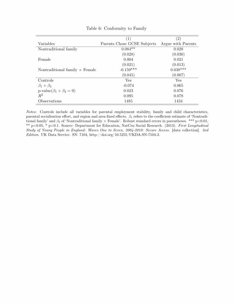
Table 6: Conformity to Family

(1) (2)Variables Parents Chose GCSE Subjects Argue with ParentsNontraditional family 0.084** 0.028

(0.028) (0.030)Female 0.004 0.021

(0.021) (0.013)Nontraditional family × Female -0.159*** 0.038***

(0.045) (0.007)Controls Yes Yesβ1 + β3 -0.074 0.065p-value(β1 + β3 = 0) 0.023 0.076R2 0.095 0.078Observations 1485 1434

Notes: Controls include all variables for parental employment stability, family and child characteristics,parental socialisation effort, and region and area fixed effects. β1 refers to the coefficient estimate of ‘Nontradi-tional family’ and β3 of ‘Nontraditional family × Female’. Robust standard errors in parentheses. *** p<0.01,** p<0.05, * p<0.1. Source: Department for Education, NatCen Social Research. (2013). First LongitudinalStudy of Young People in England: Waves One to Seven, 2004-2010: Secure Access. [data collection]. 2ndEdition. UK Data Service. SN: 7104, http://doi.org/10.5255/UKDA-SN-7104-2.

Table 7: RD Results: Nontraditional Family Treatment Effect

(1) (2) (3) (4)Panel A: Parents Chose GCSE Subjects

Unrestricted BW -0.349*** -0.398*** -0.349*** -0.467***(0.075) (0.103) (0.085) (0.119)

Optimal BW -0.495*** -0.653*** -0.408** -0.588**(0.170) (0.238) (0.162) (0.235)

Observations 560 560 559 559Controls No No Yes Yes1st-order Polynomial Yes No Yes No2nd-order Polynomial No Yes No Yes

Panel B: Argue with ParentsUnrestricted BW 0.157* 0.275** 0.183* 0.236*

(0.090) (0.128) (0.101) (0.140)Optimal BW 0.420*** 0.311 0.295** 0.374**

(0.142) (0.205) (0.142) (0.173)Observations 552 552 551 551Controls No No Yes Yes1st-order Polynomial Yes No Yes No2nd-order Polynomial No Yes No Yes

Notes: Controls include all variables for parental employment stability, family and child characteristics,parental socialisation effort, region and area fixed effects. Robust standard errors in parentheses. *** p<0.01,** p<0.05, * p<0.1. Source: Department for Education, NatCen Social Research. (2013). First LongitudinalStudy of Young People in England: Waves One to Seven, 2004-2010: Secure Access. [data collection]. 2ndEdition. UK Data Service. SN: 7104, http://doi.org/10.5255/UKDA-SN-7104-2.

34

Figure 1: Social Norms and Gender Inequality

(a) Gender Pay Gap

AT

AUCZ

DE

DK

FI

FR

GB

HU

IL

JP

NL

NO

SE

SK

US

b = 0.551(0.233)

1015

2025

3035

Mal

e-Fe

mal

e G

ap in

Med

ian

Wag

e (%

)

40 45 50 55 60% Against Women Working Full-time

(b) labor Supply: Extensive Margin

AT

AUBR

CL

CZDE

DK

ES

FI

FR

GB

HU

IEIL JP

MX

NL

NO

PL

PT RU

SE

SISK

US

b = -0.395(0.119)

3540

4550

5560

Fem

ale

LFP

(%)

30 40 50 60 70 80% Against Women Working Full-time

(c) labor Supply: Intensive Margin

AT

AU

DE

DK ES

FI

FR

GB

HU

JP

MX

NL

NO

PL

PT

SE

SI US b = -0.833(0.206)

4050

6070

80Fe

mal

e-M

ale

Hou

rs G

ap (%

)

30 40 50 60 70 80% Against Women Working Full-time

Notes: This figure shows, for various OECD countries, the relationship between the proportion stating thatwomen should not work full-time (horizontal axis) and three labor market outcomes (vertical axis). The figuresare based on data from the 2002 International Social Survey Programme and OECD statistics. Source: ISSPResearch Group (2013): International Social Survey Programme: Family and Changing Gender Roles III -ISSP 2002. GESIS Data Archive, Cologne. ZA3880 Data file Version 1.1.0, doi:10.4232/1.11564.

Figure 2: The Social Norm

(a) No children

98.08

1.31 0.61

020

4060

8010

0

Full-Time Part-Time Home

Men

81.91

9.44 8.65

020

4060

8010

0

Full-Time Part-Time Home

Women

(b) Have child under school age

94.53

2.84 2.63

020

4060

8010

0

Full-Time Part-Time Home

Men

14.48

32.79

52.73

020

4060

8010

0

Full-Time Part-Time Home

Women

(c) Youngest child still in school

95.19

2.86 1.95

020

4060

8010

0

Full-Time Part-Time Home

Men

21.30

52.86

25.84

020

4060

8010

0

Full-Time Part-Time Home

Women

(d) Children left the home

94.52

2.40 3.08

020

4060

8010

0

Full-Time Part-Time Home

Men

46.18

38.89

14.93

020

4060

8010

0Full-Time Part-Time Home

Women

Notes: This figure shows the labor supply of men and women in heterosexual couples, using data from the2002 International Social Survey Programme. It plots the proportion of men and women working full-time,part-time or not at all in each of the following cases: (a) when they have no children, (b) when they havea child under school age (i.e. below 4), (c) when their youngest child is above 4 but still within schoolingage, and (d) when their children have grown up and left the home. Source: ISSP Research Group (2013):International Social Survey Programme: Family and Changing Gender Roles III - ISSP 2002. GESIS DataArchive, Cologne. ZA3880 Data file Version 1.1.0, doi:10.4232/1.11564.

36

Figure 3: The Distribution of the Mother’s Income Share: Next Steps

McCrary Test:Discontinuity est.= -.004(.281)

050

100

150

Num

ber o

f Obs

erva

tions

per

Bin

0 .1 .2 .3 .4 .5 .6 .7 .8 .9 1Mother's Income Share

Notes: This figure plots the distribution of the assignment variable (mother’s income share) in the NextSteps data, using a bin size of 0.02. It also shows the results from a McCrary test, which tests the null ofno discontinuity at the 0.5 threshold (vertical line) of the assignment variable. The null of no discontinuitycannot be rejected at the 10% level. Source: Department for Education, NatCen Social Research. (2013).First Longitudinal Study of Young People in England: Waves One to Seven, 2004-2010: Secure Access. [datacollection]. 2nd Edition. UK Data Service. SN: 7104, http://doi.org/10.5255/UKDA-SN-7104-2.

37

Figure 4: The Distribution of the Wife’s Income Share: Further Datasets

(a) Family Resources Survey (FRS)

McCrary Test:Discontinuity est.= .107(.042)

050

010

0015

0020

00N

umbe

r of O

bser

vatio

ns p

er B

in

0 .1 .2 .3 .4 .5 .6 .7 .8 .9 1Mother's Income Share

(b) Survey of Personal Incomes (SPI)

McCrary Test:Discontinuity est.= -.579(.07)

020

040

060

0N

umbe

r of O

bser

vatio

ns p

er B

in

0 .1 .2 .3 .4 .5 .6 .7 .8 .9 1Wife's Income Share

(c) FRS - Families with Self-Employment In-come

McCrary Test:Discontinuity est.= .614(.111)

010

020

030

0N

umbe

r of O

bser

vatio

ns p

er B

in

0 .1 .2 .3 .4 .5 .6 .7 .8 .9 1Mother's Income Share

(d) SPI - Families with Self-Employment In-come

McCrary Test:Discontinuity est.= -.886(.094)

010

020

030

040

0N

umbe

r of O

bser

vatio

ns p

er B

in

0 .1 .2 .3 .4 .5 .6 .7 .8 .9 1Wife's Income Share

(e) FRS - Families with only Wage Income

McCrary Test:Discontinuity est.= -.006(.048)

050

010

0015

0020

00N

umbe

r of O

bser

vatio

ns p

er B

in

0 .1 .2 .3 .4 .5 .6 .7 .8 .9 1Mother's Income Share

(f) SPI - Families with only Wage Income

McCrary Test:Discontinuity est.= -.132(.121)

020

040

060

0N

umbe

r of O

bser

vatio

ns p

er B

in

0 .1 .2 .3 .4 .5 .6 .7 .8 .9 1Wife's Income Share

Notes: These figures plot the distribution of the assignment variable across different samples. Figures (a),(c) and (e) are from the Family Resources Survey, and (b), (d) and (f) from the Survey of Personal Incomes.Figures (a) and (b) include all families, (c) and (d) only those with self-employment income, and (e) and(f) those with only wage income. The bin size is 0.02. Each figure reports the result of the McCrary test,which tests the null of no discontinuity at the 0.5 threshold (vertical line) of the assignment variable. Sources:Department of Work and Pensions, Office for National Statistics. Social and Vital Statistics Division, NatCenSocial Research. (2016). Family Resources Survey. UK Data Service, and Inland Revenue. Statistics Division.(1989). Survey of Personal Incomes, 1985-1986: Public Use Tape. UK Data Service.

38

Figure 5: Regression Discontinuity Graphs: Conformity to Family

(a) Parents Chose GCSE Subjects

0.2

.4.6

.81

0 .1 .2 .3 .4 .5 .6 .7 .8 .9 1Mother's Income Share

(b) Argue with Parents

0.2

.4.6

.81

0 .1 .2 .3 .4 .5 .6 .7 .8 .9 1Mother's Income Share

Notes: The figure shows, for females, the probability that they agree with each of the two conformity measures,above and below the 0.5 cutoff. The first is whether children chose what GCSE subjects to study based onwhat their parents wanted, and the second is whether children argue with their parents. Observations aredivided into bins of width 0.05. Source: Department for Education, NatCen Social Research. (2013). FirstLongitudinal Study of Young People in England: Waves One to Seven, 2004-2010: Secure Access. [datacollection]. 2nd Edition. UK Data Service. SN: 7104, http://doi.org/10.5255/UKDA-SN-7104-2.

39

Figure 6: Placebo Tests

(a) Parents Chose GCE Subjects

True Cutoff at 0.5

-1-.5

0.5

1

0.1 0.15 0.2 0.25 0.3 0.35 0.4 0.45 0.5 0.55 0.6Mother's Income Share as Placebo Cutoff for Treatment

(b) Argue with Parents

True Cutoff at 0.5

-2-1

01

2

0.1 0.15 0.2 0.25 0.3 0.35 0.4 0.45 0.5 0.55 0.6Mother's Income Share as Placebo Cutoff for Treatment

Notes: These figures show estimates of jumps in the outcome variable, and their associated 95% confidenceintervals, for a wide range of placebo treatment cutoffs between 0.1 and 0.6 of the mother’s income share. Thedashed grey line marks the true cutoff at 0.5. Source: Department for Education, NatCen Social Research.(2013). First Longitudinal Study of Young People in England: Waves One to Seven, 2004-2010: Secure Access.[data collection]. 2nd Edition. UK Data Service. SN: 7104, http://doi.org/10.5255/UKDA-SN-7104-2.

40

FOR ONLINE PUBLICATION

Appendix A. Further Predictions of the ModelSection 3 presented a simple model of gender identity. It was shown that children choose theiroptimal belief about gender roles using the following rule:

x∗ = argmaxx

U = x(xF,xS, Z) =cF (xF , xS, Z)xF + cS(xF , xS, Z)xScF (xF , xS, Z) + cS(xF , xS, Z)

(A.1)

The main text focused on ∂x∗

∂cFand showed that this prediction holds in the data. In this

appendix I briefly discuss another comparative static and show that it also confirmed by theempirical results. Here I look at ∂x∗

∂xF, i.e. how living in a more traditional family changes the

child’s optimal belief. Recall that higher values of x∗, xF and xS indicate more traditionalvalues, and that in the empirical specification, xS > xF . Given this setup, the prediction is22:

∂x∗

∂xF=[(cF (xF , xS, Z) + cS(xF , xS, Z))

2]×[

c2F (xF , xS, Z) + cF (xF , xS, Z)cS(xF , xS, Z)+

(xS − xF )(cF (xF , xS, Z)

∂cS∂xF

− cS(xF , xS, Z)∂cF∂xF

)](A.2)

The sign of (A.2) depends on the signs of both ∂cS∂xF

and ∂cF∂xF

. While there is no proxyin the data to estimate ∂cS

∂xF, the evidence from the social psychology literature (Asch 1951;

1952; etc.) implies ∂cS∂xF≥ 0. The reasoning is as follows. The literature has established that

individuals have strong preferences for conforming to society. Furthermore, the social normregarding gender roles in the UK is very traditional. Hence, the more traditional a family’sgender norm is, the more the family norm aligns with the social norm that individuals havea strong preference to conform to. Hence, the strength of their preference for conforming tothe social norm must be non-decreasing in xF .

The prediction therefore ultimately depends on the sign of ∂cF∂xF

, which can be estimatedfrom the data. In Section 6, I found that ∂x∗

∂xF> 0 for boys, and ∂x∗

∂xF< 0 for girls. To show that

these empirical results are consistent with the model, first consider boys. A sufficient conditionfor ∂x∗

∂xF> 0 is ∂cF

∂xF< 0, i.e. that boys in nontraditional families have stronger preferences for

conforming to their family than boys in traditional families. The results of Table 6 confirmthis. The coefficient on the ‘Nontraditional family’ dummy is positive, confirming that boysin such families have stronger preferences for conformity.

Now consider the prediction for girls. A necessary (though not sufficient condition) for∂x∗

∂xF< 0 is ∂cF

∂xF> 0, i.e. that girls in nontraditional families have weaker preferences for

conforming to their family than girls in traditional families. This was the focus of all ofSection 7, which confirmed this weaker preference.

22Here I have for simplicity assumed that the family norm does not depend on the social norm. Introducingthis dependence does not change the prediction.

41

Appendix B. Discussion of CovariatesAs discussed in Section 5.3, the main regressions include controls for family, child and geo-graphical characteristics, and proxies for parental-socialization effort. The aim is to control,as much as possible, for variables that are correlated with both the child expressing traditionalviews and living in a nontraditional family. In what follows I explain in more detail whichvariables I control for and why I consider it important to do so in the context of my researchquestion.

The family characteristics of immediate concern are cultural and socio-economic attributes.A key variable controlled for is parental religion. As religions offer various prescriptions onthe appropriate behavior of individuals in society, including gender roles, parents’ religiousviews can affect not only how much mothers work and earn, but also the way parents socializetheir children (Guiso et al. 2003; Lehrer 1995). Moreover, this effect may depend on howimportant religion is to the parents’ way of life; religious parents are more likely than non-practising individuals to conform to the gender roles prescribed by their religion (Guiso et al.2003; Heineck 2004). I account for this by controlling for the strength of parental religiosity.I also control for whether a child has ever attended a religious or single-sex school, as bothreflect parents’ related social preferences.

To account for family structure, I control for whether the child lives with her biologicalparents and whether the parents are married. Evidence (Parker and Wang 2013) shows thatmarital status affects parents’ beliefs about the ideal relative labor supply, which may deter-mine who the breadwinner is. Growing up in a ‘non-conventional’ family of unmarried parentsmay, however, also affect how children view social norms, thereby affecting their preference forconformity to them. For instance, living in a ‘non-conventional’ family can affect the extent towhich children consider social norms (which the parents are not following) desirable. Indeed, apositive relation between living in ‘non-conventional’ families and adopting ‘non-conventional’norms is found by Hognas and Carlson (2012), who show that children raised by unmarriedparents have a higher likelihood of non-marital childbearing in adulthood.

To further account for family structure, I also control for household size. Larger householdsimply a higher financial burden and, therefore, a greater likelihood that both parents areworking. Nonetheless, larger households (and, hence, more siblings, chores, and so forth) totake care of may increase the need for the child’s contribution to household tasks, therebyaffecting the child’s belief about her gender’s role within the family.

Among parent-specific characteristics, parental age is a crucial factor that needs to beaccounted for. As age increases, so does the probability that a parent is working. Moreover,due to the stylized fact of a concave earnings profile over the life cycle (Polachek 2008),earnings also increase with age for working adults. I therefore control for parental age becauseit directly affects the relative family labor supply and income.

I also control for parental education, social class and total family income. Education notonly increases earnings through higher human capital (Becker 1964) but can also directlyaffect social attitudes; higher education is associated with more liberal social views (Dee 2004;Stankov 2009; Kanazawa 2010). The same holds for social class. Although higher class statushas historically been associated with more conservative beliefs, social class in modern times(as measured by the Goldthorpe scale using occupation types) captures job prestige and ishighly correlated with education. For instance, Guiso et al. (2003) find that higher income

42

(which is associated with social class, as this is defined by occupation) leads to more liberalviews on gender equality. Thus, I expect income to have similar effects as education.

To better capture between-family income heterogeneity, I include an additional variable:the Index of Multiple Deprivation (IMD). This is defined at the Super Output Area (SOA)level. SOAs divide England into 32,482 local geographical districts - each the size of a neigh-borhood - and has been devised to improve the reporting of small-area statistics by the UKOffice of National Statistics. The IMD accounts for deprivation in the following dimensions:income, employment, health and disability, education skills and training, barriers to housingand services, crime, and living environment23. The most deprived SOA is given an IMD rankof 1, and the least deprived a rank of 32,482.

Geographic characteristics may also confound my results and are therefore controlled for.The region and type of area (urban versus rural) may affect the employment opportunitiesand thus relative earnings of mothers. In addition, areas may vary in how traditional ormodern the prevailing local norms are. For instance, larger and more urban areas are usuallyassociated with more secular and liberal views (Maneschiold and Haraldsson 2007).

Besides family and geographic characteristics, I also account for between-child heterogene-ity. First, I control for ethnicity. Research shows that ethnicity has an important effect onattitudes towards gender roles (Kane 2000). Compared to non-whites, whites are more criti-cal of maternal employment and consider it more harmful for young children (Dugger 1988).Beyond ethnicity, I also control for whether the child was born in the UK, the child’s religionand the importance of religion to her life.

Furthermore, child characteristics related to cognitive abilities may also have a confoundingeffect. Research relates higher intelligence to more socially liberal views (Deary et al. 2008);evidence also shows that low birth weight is associated with development delays and therebylower intellectual capacity (Ramey et al. 1999). Since the data do not contain objectivemeasures of innate ability, the best way to control for this possible confounder is to indirectlyaccount for it by controlling for birth weight. Further proxies are also available in the data,such as whether the child has special education needs and disabilities. All of these variablesare included to control for cognitive abilities as accurately as possible.

Last, as I am interested in examining how successfully parents socialize their children,I account for an important determinant of success: parental effort in socialization. Sinceno perfect measure exists, I use proxies capturing the quality and quantity of contact timebetween parents and children, which has been emphasized in the literature as an importantfactor in gender stereotyping (Bem 1985; Cooksey and Fondell 1996; Asgari et al. 2010; Carrellet al. 2010). For more details of these proxies, see Table C.3 in Appendix C.

23For a more detailed explanation of this index, see Neighborhood Renewal Unit (2004).

43

Appendix C. Extra Tables

Table C.1: Summary Statistics: Original Vs Final Sample (Next Steps)

Initial Sample Final SampleVariables Mean s.d. Mean s.d.Nontraditional family 0.143 0.35 0.145 0.352Mother’s income share 0.279 0.254 0.287 0.251Traditional norm 0.349 0.477 0.311 0.463High wage important 0.656 0.475 0.641 0.48Want to study science 0.399 0.49 0.409 0.492Parents chose GCSE subjects 0.359 0.48 0.374 0.484Argue with parents 0.578 0.494 0.605 0.489Female 0.516 0.500 0.524 0.500Observations 8682 1487

Notes: Table shows summary statistics for the main variables of interest, comparing those from the orig-inal sample to those used in the final sample after imposing sample restrictions. Source: Department forEducation, NatCen Social Research. (2013). First Longitudinal Study of Young People in England: WavesOne to Seven, 2004-2010: Secure Access. [data collection]. 2nd Edition. UK Data Service. SN: 7104,http://doi.org/10.5255/UKDA-SN-7104-2.

Table C.2: Summary Statistics of FRS and SPI data

Family Resources Survey Survey of Personal IncomesVariables Mean s.d. Mean s.d.Husband’s earnings 27688.06 36409.41 12801.77 12436.70Wife’s earnings 10503.26 12134.18 1500.54 3804.62Wife’s share 0.29 0.22 0.08 0.16Self-employment 0.22 0.47 0.28 0.45Years 1997-2004 1985-1986Observations 33309 38979

Notes: Summary statistics for the Family Resources Survey and the Survey of Personal Incomes datasets.Sources: Department of Work and Pensions, Office for National Statistics. Social and Vital Statistics Division,NatCen Social Research. (2016). Family Resources Survey. UK Data Service, and Inland Revenue. StatisticsDivision. (1989). Survey of Personal Incomes, 1985-1986: Public Use Tape. UK Data Service.

44

Table C.3: Summary Statistics

Variable Description Mean s.d.Nontraditional family 1 if mother earns more than father 0.145 0.352Mother’s income share Mother’s income divided by family income 0.287 0.251Traditional norm 1 if child agrees that women should never work 0.311 0.463

full-time when they have young childrenHigh wage important 1 if child believes that having a job that pays 0.641 0.480

well is importantWant to study science 1 if child wants to study science at university 0.409 0.492Parents chose GCSE subjects 1 if child studied what her parents wanted at GCSE 0.374 0.484Argue with parents 1 if child argues with parents 0.605 0.489Parents not married 1 if child’s parents are not married 0.059 0.236Both parents biological 1 if both are child’s biological parents 0.894 0.307Household size No. of people in child’s household 4.593 1.119Father age Father’s age in years 42.843 5.252Mother age Mother’s age in years 44.379 6.032Religion important to parents 1 if parents state religion is important to 0.582 0.493

their way of lifeFather religion: muslim 1 if father is Muslim 0.076 0.265Father religion: minority 1 if father is Sikh, Hindu, Buddhist, 0.075 0.263

Jewish, AtheistMother religion: muslim 1 if mother is Muslim 0.078 0.268Mother religion: minority 1 if mother is Sikh, Hindu, Buddhist, 0.179 0.383

Jewish, AtheistFamily education: below degree 1 if highest education between parents is 0.202 0.401

higher education below degree levelFamily education: GCE A Level 1 if highest education between parents is 0.210 0.407

GCE A Level or equivalent (post-compulsory)Family education: GCSE 1 if highest education between parents is 0.238 0.426

GCSE level grades A-C, or equivalentFamily education: level 1 1 if highest education between parents is 0.036 0.187

at vocation level/GCSE grades D- or equivalentFamily education: other 1 if highest education between parents is informal 0.009 0.097Family education: none 1 if neither parent has any education qualifications 0.059 0.236Father SC: lower manag. 1 if father’s occupation is Lower Managerial 0.297 0.457

or ProfessionalFather SC: intermediate 1 if father’s occupation is Intermediate 0.177 0.382Father SC: small employer 1 if father’s occupation is Small Employer 0.038 0.192

or Own Accounts WorkerFather SC: lower supervisor 1 if father’s occupation is Lower Supervisory 0.085 0.279

or TechnicalFather SC: semi-routine 1 if father’s occupation is Semi-Routine 0.206 0.405Father SC: routine 1 if father’s occupation is Routine 0.087 0.283Father SC: long-term u/e 1 if father is long-term unemployed/never worked 0.031 0.173Mother SC: lower manag. 1 if mother’s occupation is Lower Managerial 0.258 0.438

or ProfessionalMother SC: intermediate 1 if mother’s occupation is Intermediate 0.077 0.266Mother SC: small employer 1 if mother’s occupation is Small Employer 0.079 0.270

or Own Accounts WorkerMother SC: lower supervisor 1 if mother’s occupation is Lower Supervisory 0.144 0.351

or TechnicalMother SC: semi-routine 1 if mother’s occupation is Semi-Routine 0.102 0.302Mother SC: routine 1 if mother’s occupation is Routine 0.118 0.322

45

Continuation of Table C.3Variable Description Mean s.d.Mother SC: long-term u/e 1 if mother is long-term unemployed/never worked 0.048 0.213Father employment: stable 1 if father did not change employment 5 years 0.751 0.433

before wave 1 up to wave 4Mother employment: stable 1 if mother did not change employment 5 years 0.480 0.500

before wave 1 up to wave 4Mother more educated 1 if mother has higher level of education 0.293 0.455

than fatherMother higher job status 1 if mother has higher job status level 0.497 0.500

than father(defined by occupation type)

Family income Total annual family income 39.964 31.855(sum of father’s and mother’s income)

Rank of IMD Rank of Index of Multiple Deprivation 17577.731 9427.898Female 1 if child is female 0.524 0.500Child born in UK 1 if child was born in the UK 0.962 0.190Child ethnicity: mixed 1 if child’s ethnicity is mixed 0.024 0.152Child ethnicity: indian 1 if child’s ethnicity is Indian 0.074 0.262Child ethnicity: pakistani 1 if child’s ethnicity is Pakistani 0.043 0.203Child ethnicity: bangladeshi 1 if child’s ethnicity is Bagladeshi 0.015 0.121Child ethnicity: black caribbean 1 if child’s ethnicity is Black Caribbean 0.011 0.103Child ethnicity: black african 1 if child’s ethnicity is Black African 0.014 0.118Child ethnicity: other 1 if child’s ethnicity is none of above 0.022 0.147Religion important to child 1 if child states that religion is important to 0.165 0.372

her way of lifeChild religion: muslim 1 if child is Muslim 0.077 0.267Child religion: minority 1 if child is Sikh, Hindu, Buddhist, 0.124 0.330

Jewish, AtheistChild birth weight Child birth weight in kg 3.317 0.594Child has SEN statement 1 if child has Special Education Needs 0.139 0.346Child has disability 1 if child has a disability 0.028 0.166Ever attended single sex school 1 if child ever attended a single sex school 0.137 0.343Ever attended religious school 1 if child ever attended a religious school 0.160 0.367Family evenings: often 1 if parents spend evenings with child 0.941 0.236

at least 3 times per monthFamily evenings: sometimes 1 if parents spend evenings with child 0.028 0.166

once per month or lessCurfew: always 1 if parents always set curfew for child 0.968 0.175Family activities: often 1 if go out together as family 0.905 0.294

at least 3 times per monthFamily activities: sometimes 1 if go out together as family 0.079 0.270

once per month or lessTalk about school: often 1 if parents frequently talk to child 0.485 0.500

about school dayNorth East 1 if child grew up in the North East 0.062 0.241North West 1 if child grew up in the North West 0.150 0.357Yorkshire and the Humber 1 if child grew up in Yorkshire and the Humber 0.102 0.303East Midlands 1 if child grew up in East Midlands 0.093 0.290West Midlands 1 if child grew up in West Midlands 0.135 0.342East of England 1 if child grew up in the East of England 0.104 0.305London 1 if child grew up in London 0.106 0.307South East 1 if child grew up in the South East 0.159 0.366South West 1 if child grew up in the South West 0.090 0.286Urban 1 if child grew up in an urban area 0.787 0.410

46

Continuation of Table C.3Variable Description Mean s.d.Town 1 if child grew up in a town 0.089 0.285Village 1 if child grew up in a village 0.081 0.272Hamlet 1 if child grew up in a hamlet 0.026 0.158

(smaller than a village)

Source: Department for Education, NatCen Social Research. (2013). First Longitudinal Study of Young Peoplein England: Waves One to Seven, 2004-2010: Secure Access. [data collection]. 2nd Edition. UK Data Service.SN: 7104, http://doi.org/10.5255/UKDA-SN-7104-2.

47

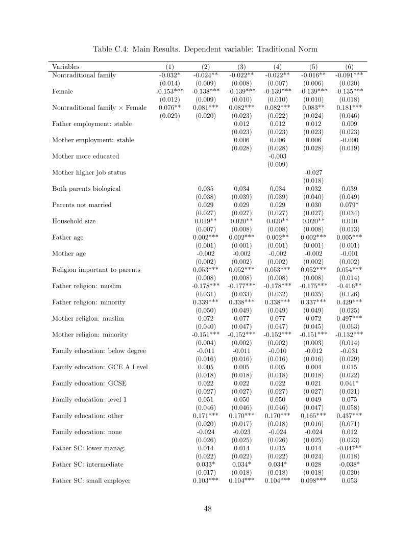
Table C.4: Main Results. Dependent variable: Traditional Norm

Variables (1) (2) (3) (4) (5) (6)Nontraditional family -0.032* -0.024** -0.022** -0.022** -0.016** -0.091***

(0.014) (0.009) (0.008) (0.007) (0.006) (0.020)Female -0.153*** -0.138*** -0.139*** -0.139*** -0.139*** -0.135***

(0.012) (0.009) (0.010) (0.010) (0.010) (0.018)Nontraditional family × Female 0.076** 0.081*** 0.082*** 0.082*** 0.083** 0.181***

(0.029) (0.020) (0.023) (0.022) (0.024) (0.046)Father employment: stable 0.012 0.012 0.012 0.009

(0.023) (0.023) (0.023) (0.023)Mother employment: stable 0.006 0.006 0.006 -0.000

(0.028) (0.028) (0.028) (0.019)Mother more educated -0.003

(0.009)Mother higher job status -0.027

(0.018)Both parents biological 0.035 0.034 0.034 0.032 0.039

(0.038) (0.039) (0.039) (0.040) (0.049)Parents not married 0.029 0.029 0.029 0.030 0.079*

(0.027) (0.027) (0.027) (0.027) (0.034)Household size 0.019** 0.020** 0.020** 0.020** 0.010

(0.007) (0.008) (0.008) (0.008) (0.013)Father age 0.002*** 0.002*** 0.002** 0.002*** 0.005***

(0.001) (0.001) (0.001) (0.001) (0.001)Mother age -0.002 -0.002 -0.002 -0.002 -0.001

(0.002) (0.002) (0.002) (0.002) (0.002)Religion important to parents 0.053*** 0.052*** 0.053*** 0.052*** 0.054***

(0.008) (0.008) (0.008) (0.008) (0.014)Father religion: muslim -0.178*** -0.177*** -0.178*** -0.175*** -0.416**

(0.031) (0.033) (0.032) (0.035) (0.126)Father religion: minority 0.339*** 0.338*** 0.338*** 0.337*** 0.429***

(0.050) (0.049) (0.049) (0.049) (0.025)Mother religion: muslim 0.072 0.077 0.077 0.072 0.497***

(0.040) (0.047) (0.047) (0.045) (0.063)Mother religion: minority -0.151*** -0.152*** -0.152*** -0.151*** -0.132***

(0.004) (0.002) (0.002) (0.003) (0.014)Family education: below degree -0.011 -0.011 -0.010 -0.012 -0.031

(0.016) (0.016) (0.016) (0.016) (0.029)Family education: GCE A Level 0.005 0.005 0.005 0.004 0.015

(0.018) (0.018) (0.018) (0.018) (0.022)Family education: GCSE 0.022 0.022 0.022 0.021 0.041*

(0.027) (0.027) (0.027) (0.027) (0.021)Family education: level 1 0.051 0.050 0.050 0.049 0.075

(0.046) (0.046) (0.046) (0.047) (0.058)Family education: other 0.171*** 0.170*** 0.170*** 0.165*** 0.437***

(0.020) (0.017) (0.018) (0.016) (0.071)Family education: none -0.024 -0.023 -0.024 -0.024 0.012

(0.026) (0.025) (0.026) (0.025) (0.023)Father SC: lower manag. 0.014 0.014 0.015 0.014 -0.047**

(0.022) (0.022) (0.022) (0.024) (0.018)Father SC: intermediate 0.033* 0.034* 0.034* 0.028 -0.038*

(0.017) (0.018) (0.018) (0.018) (0.020)Father SC: small employer 0.103*** 0.104*** 0.104*** 0.098*** 0.053

48

Continuation of Table C.4Variables (1) (2) (3) (4) (5) (6)

(0.027) (0.027) (0.027) (0.026) (0.040)Father SC: lower supervisor 0.051 0.052 0.052 0.046 -0.035

(0.029) (0.031) (0.031) (0.031) (0.045)Father SC: semi-routine 0.127*** 0.128*** 0.128*** 0.115*** 0.093***

(0.013) (0.011) (0.011) (0.016) (0.018)Father SC: routine 0.149*** 0.150*** 0.149*** 0.136*** 0.121*

(0.024) (0.025) (0.025) (0.025) (0.051)Father SC: long-term u/e 0.118*** 0.118*** 0.118*** 0.100***

(0.017) (0.016) (0.016) (0.013)Mother SC: lower manag. 0.020 0.020 0.021 0.028* 0.034**

(0.011) (0.011) (0.011) (0.014) (0.010)Mother SC: intermediate 0.050** 0.050** 0.051** 0.060** 0.109***

(0.014) (0.014) (0.015) (0.017) (0.020)Mother SC: small employer 0.114*** 0.116*** 0.117*** 0.127*** 0.123***

(0.027) (0.026) (0.024) (0.021) (0.032)Mother SC: lower supervisor 0.012 0.014 0.015 0.026 0.017

(0.017) (0.017) (0.017) (0.021) (0.012)Mother SC: semi-routine 0.055 0.057* 0.058* 0.071** 0.067**

(0.031) (0.029) (0.027) (0.023) (0.025)Mother SC: routine 0.059* 0.061* 0.062** 0.080** 0.112**

(0.027) (0.027) (0.026) (0.025) (0.039)Mother SC: long-term u/e -0.003 -0.002 -0.002 0.001

(0.041) (0.040) (0.039) (0.039)Family income -0.000* -0.000* -0.000* -0.000* -0.000

(0.000) (0.000) (0.000) (0.000) (0.000)Rank of IMD -0.000 -0.000 -0.000 -0.000 -0.000

(0.000) (0.000) (0.000) (0.000) (0.000)Child born in UK -0.064* -0.065** -0.065** -0.066** -0.097**

(0.031) (0.026) (0.026) (0.025) (0.038)Child ethnicity: mixed -0.049*** -0.049*** -0.049*** -0.045*** -0.101***

(0.010) (0.007) (0.007) (0.007) (0.005)Child ethnicity: indian -0.217*** -0.216*** -0.216*** -0.216*** -0.297***

(0.024) (0.025) (0.024) (0.025) (0.044)Child ethnicity: bangladeshi -0.163*** -0.163*** -0.163*** -0.161*** -0.430***

(0.016) (0.015) (0.015) (0.015) (0.049)Child ethnicity: black caribbean -0.196*** -0.200*** -0.199*** -0.203*** -0.191***

(0.007) (0.013) (0.013) (0.015) (0.014)Child ethnicity: black african 0.101*** 0.104*** 0.103*** 0.101*** -0.037***

(0.021) (0.028) (0.026) (0.026) (0.010)Child ethnicity: other 0.023 0.024 0.024 0.019 -0.126***

(0.032) (0.033) (0.032) (0.031) (0.035)Religion important to child 0.080*** 0.080*** 0.080*** 0.080*** 0.055

(0.017) (0.016) (0.016) (0.016) (0.033)Child religion: muslim 0.068 0.063 0.063 0.064

(0.050) (0.057) (0.058) (0.058)Child religion: minority -0.038 -0.039 -0.038 -0.039 -0.063***

(0.049) (0.051) (0.050) (0.050) (0.013)Child birth weight -0.009 -0.009 -0.009 -0.009 -0.018

(0.011) (0.011) (0.011) (0.011) (0.011)Child has SEN statement 0.076*** 0.077*** 0.077*** 0.078*** 0.062**

(0.017) (0.019) (0.019) (0.020) (0.020)Child has disability 0.005 0.007 0.007 0.008 0.039

(0.041) (0.038) (0.038) (0.038) (0.043)

49

Continuation of Table C.4Variables (1) (2) (3) (4) (5) (6)Ever attended single sex school -0.002 -0.001 -0.001 -0.001 -0.008

(0.011) (0.011) (0.011) (0.011) (0.020)Ever attended religious school -0.011 -0.012 -0.012 -0.011 -0.007

(0.013) (0.014) (0.014) (0.013) (0.012)Family evenings: often -0.014 -0.015 -0.015 -0.015 -0.005

(0.057) (0.058) (0.058) (0.059) (0.071)Family evenings: sometimes -0.126 -0.128 -0.128 -0.128 -0.096

(0.083) (0.085) (0.085) (0.086) (0.088)Curfew: always 0.107 0.108 0.108 0.107 0.115

(0.058) (0.059) (0.059) (0.060) (0.107)Family activities: often 0.015 0.014 0.014 0.008 0.106

(0.074) (0.074) (0.074) (0.070) (0.099)Family activities: sometimes 0.046 0.044 0.044 0.040 0.109

(0.083) (0.081) (0.081) (0.079) (0.099)Talk about school: often -0.013 -0.013 -0.013 -0.014 -0.004

(0.011) (0.011) (0.011) (0.011) (0.018)β1 + β3 0.044 0.056 0.060 0.060 0.066 0.090p-value(β1 + β3 = 0) 0.11 0.0022 0.0076 0.011 0.02 0.061R2 0.024 0.11 0.11 0.11 0.12 0.13Observations 1487 1485 1485 1485 1485 1125

Notes: The table shows the coefficient estimates for various versions of the main specification, where differentcontrols are included. Column (6) runs the same specification as shown in (3) but on the subsample offamilies where both parents work. β1 refers to the coefficient estimate of ‘Nontraditional family’ and β3 of‘Nontraditional family × Female’. Robust standard errors in parentheses. *** p<0.01, ** p<0.05, * p<0.1.Source: Department for Education, NatCen Social Research. (2013). First Longitudinal Study of Young Peoplein England: Waves One to Seven, 2004-2010: Secure Access. [data collection]. 2nd Edition. UK Data Service.SN: 7104, http://doi.org/10.5255/UKDA-SN-7104-2.

50

Table C.5: Covariate Balance Tests

(1) (2)Variables Point Estimate s.e.Both parents biological -0.084 0.103Parents not married 0.104 0.089Household size -0.81** 0.396Father age -2.118 1.48Mother age -1.62 2.215Religion important to parents 0.152 0.238Father religion: muslim 0.066 0.106Father religion: minority -0.048 0.105Mother religion: muslim 0.066 0.106Mother religion: minority -0.017 0.15Family education: below degree 0.260** 0.128Family education: GCE A Level -0.214 0.139Family education: GCSE -0.141 0.095Family education: level 1 -0.013 0.014Family education: other -0.019 0.02Family education: none -0.132 0.118Father SC: lower manag. 0.432*** 0.133Father SC: intermediate 0.111** 0.048Father SC: lower supervisor -0.151** 0.076Father SC: semi-routine -0.028 0.063Father SC: routine -0.162 0.124Mother SC: lower manag. 0.211 0.196Mother SC: intermediate 0.096 0.111Mother SC: lower supervisor -0.239* 0.127Mother SC: semi-routine -0.084 0.086Mother SC: routine -0.145 0.157Family income 13.595 9.311Rank of IMD 997.992 3534.826Child born in UK -0.263* 0.145Child ethnicity: mixed 0.125 0.11Child ethnicity: indian -0.055 0.093Child ethnicity: bangladeshi 0.096 0.096Child ethnicity: black caribbean 0.027 0.095Child ethnicity: black african 0.001 0.011Child ethnicity: other -0.031 0.054Religion important to child 0 .027 0.133Child religion: muslim 0.066 0.106Child religion: minority -0.116 0.109Child birth weight -0.068 0.177Child has SEN statement 0.033 0.123Child has disability -0.029 0.074Ever attended single sex school 0.091 0.165Ever attended religious school 0.127 0.101Family evenings: often 0.189* 0.103Family evenings: sometimes -0.115 0.071Curfew: always 0.004 0.013Family activities: often 0.131 0.122Family activities: sometimes -0.225 0.147Talk about school: often 0.314 0.199North East 0.002 0.117

51

Continuation of Table C.5(1) (2)

Variables Point Estimate s.e.North West -0.125 0.139Yorkshire and the Humber -0.154 0.151East Midlands 0.156 0.105West Midlands 0.244 0.158East of England -0.136 0.136London -0.024 0.133South East -0.132* 0.073Urban 0.107 0.175Town -0.206 0.136Village 0.032 0.116Hamlet 0.001 0.002

Notes: Table shows results from balance tests on all covariates used in the main section. Robust standard errorsin parentheses. *** p<0.01, ** p<0.05, * p<0.1. Source: Department for Education, NatCen Social Research.(2013). First Longitudinal Study of Young People in England: Waves One to Seven, 2004-2010: Secure Access.[data collection]. 2nd Edition. UK Data Service. SN: 7104, http://doi.org/10.5255/UKDA-SN-7104-2.

52