brain computer interfaces using machine learning: …...brain-computer interfaces (bci’s) are new...
TRANSCRIPT

Nina Proesmans
Reducing calibration time in Motor ImageryBrain-Computer Interfaces using Machine Learning:
Academic year 2015-2016Faculty of Engineering and ArchitectureChair: Prof. dr. ir. Rik Van de WalleDepartment of Electronics and Information Systems
Master of Science in Biomedical EngineeringMaster's dissertation submitted in order to obtain the academic degree of
Counsellor: Ir. Thibault VerhoevenSupervisors: Prof. dr. ir. Joni Dambre, Dr. ir. Pieter van Mierlo

Preface
With this preface I would like to thank everyone that helped me completing this master thesis
as the finalisation of my engineering studies.
First, I would like to thank my supervisor Ir. Thibault Verhoeven, as he always made time
for questions and gave proper, enthousiastic guidance, giving me extra motivation to work
on this master thesis. I would also like to thank my promotor prof. dr. ir. Joni Dambre
for teaching me in the big and interesting world of Machine Learning and giving me the
opportunity to apply these concepts on Brain-Computer Interfaces.
Last, but definitely not least, I want to thank my parents and family for the endless support
and encouragement they gave me, making these past six years a truly great experience.

Permission for usage
The author gives permission to make this master dissertation available for consultation and
to copy parts of this master dissertation for personal use.
In the case of any other use, the copyright terms have to be respected, in particular with
regard to the obligation to state expressly the source when quoting results from this master
dissertation.
De auteur geeft de toelating deze masterproef voor consultatie beschikbaar te stellen en delen
van de masterproef te kopieren voor persoonlijk gebruik.
Elk ander gebruik valt onder de bepalingen van het auteursrecht, in het bijzonder met be-
trekking tot de verplichting de bron uitdrukkelijk te vermelden bij het aanhalen van resultaten
uit deze masterproef.
Nina Proesmans
Ghent, June 1st, 2016

Brain-Computer Interfaces using Machine
Learning: Reducing calibration time in Motor
Imagery
Nina Proesmans
Supervisors: Counsellor:
Prof. dr. ir. Joni Dambre Ir. Thibault Verhoeven
Dr. ir. Pieter van Mierlo
Master’s dissertation submitted in order to obtain the academic degree of
Master of Science in Biomedical Engineering
Faculty of Engineering and Architecture
Ghent University
Academic year 2015–2016
Department of Electronics and Information Systems
Chair: Prof. dr. ir. Rik Van de Walle
AbstractBrain-Computer Interfaces (BCI’s) are new ways for human beings to interact with a com-puter, by using only the brain. BCI’s can be very useful for people who have lost the abilityto control their limbs, as BCI’s can give these people the opportunity to, for example, steer awheelchair, using Motor Imagery. Motor Imagery is the process where the patient imaginesa movement, resulting in a signal originating from the brain and measurable through EEG.
The biggest challenge for BCI’s is that not everyone has the same brain. Using MachineLearning, for every new session, the BCI has to learn from the user’s brain, but this learningtakes time. The time that the BCI needs to adapt to the user’s brain in order to correctlyclassify their thoughts, is known as the calibration time. Up until now, this calibration couldtake up to 20 - 30 minutes, which is an exhausting and tiring amount of time that the patienthas to wait until the system is fully functional.
To solve this problem, the goal of this thesis was to reduce this calibration time as much aspossible. In the first part of this work, a first attempt is done by finding the optimal amountof features needed for reasonable functioning of the BCI, using all calibration data available.Averaged over five subjects, the amount of correctly classified thoughts only reached 67±15%.To increase the performance of the BCI while reducing the calibration time, Transfer Learningwas used. In Transfer Learning, information extracted from previously recorded subjectsis used as good as possible to reduce the amount of calibration needed for classificationof thoughts coming from a new target subject. Existing techniques were compared and anew technique was developed, resulting in the need for only 24 seconds of calibration data,classifying 86±8% of the thoughts correctly.
Keywords
Brain-Computer Interfaces, Machine Learning, Calibration time, Motor Imagery, Transfer
Learning

Brain-Computer Interfaces using MachineLearning: Reducing calibration time in
Motor ImageryNina Proesmans
Supervisor(s): Joni Dambre, Pieter van Mierlo, Thibault Verhoeven
Abstract—The goal of this article is to find a method that isable to reduce the calibration time needed for Motor Imageryclassification, without a loss of performance. For this purpose,Machine Learning is applied to the subject of Brain-ComputerInterfaces. To illustrate the level of difficulty to find a good Ma-chine Learning model that performs well for every subject, aperson-specific BCI is optimised with data available from sevensubjects. For the purpose of calibration time reduction, severalTransfer Learning techniques are exploited and a new tech-nique is proposed. The new Transfer Learning technique re-duces calibration time while performing even better.
Keywords— Brain-Computer Interfaces, Machine Learning,calibration time, Motor Imagery, Transfer Learning
I. INTRODUCTION
BY using Brain-Computer Interfaces, people whohave lost the ability to control their limbs are
given the opportunity to, for example, steer a wheel-chair by using Motor Imagery. Motor Imagery is theprocess where the patient imagines a movement, res-ulting in a signal measurable from the brain, whichis similar to the brain signals when actually planningand performing the movement [1]. In this article, ima-ginary left and right hand movement will be the topicof interest.To learn from the user’s brain, Machine Learning isapplied to Brain-Computer Interfaces. General con-cepts of different techniques needed to build a Ma-chine Learning algorithm are explained in Section II,a first BCI is built in Section III. Due to interpersonand intersession differences, the BCI needs to adaptto the user’s brain for every new session, to be ableto correctly classify their thoughts. The time that theBCI needs for this adaption is known as the calibra-tion time and up until now, this calibration could takeup to 20 - 30 minutes. With the intention of usingthese BCI’s with, for example, ALS patients, this isan exhausting and tiring amount of time that the pa-tient has to wait until the system is fully functional.To overcome this problem, several existing TransferLearning techniques are explained in Section IV. Us-ing these techniques, previously recorded data can bereused or adapted to improve prediction of tasks per-formed by new subjects. Different Transfer Learningtechniques are proposed in Section VI with their cor-responding simulations in Section V. A new Transfer
Learning technique is designed in Section VI with itsresults given in Section VII.
II. MACHINE LEARNING
Machine Learning is used to make data-drivenpredictions, based on properties of example inputs,known as the training data or training set. If an un-derlying model exists, containing the properties of thedata, a Machine Learning algorithm can construct amodel based on the available training data as close aspossible to the underlying model. If the ML algorithmsucceeded, it should be able to correctly predict classlabels of new input samples, known as the test set.Applying Machine Learning to the subject of Brain-Computer Interfaces, a set-up as in Figure 1 is used.
?Signal acquisition through EEG
Extracting important features
Fig. 1. Brain Computer Interface: Overview
Starting with different trials of imaginary move-ment of the left and right hand, the signals producedby the user are recorded using EEG. Before giving thisdata to an ML algorithm, the trials are pre-processedby filtering the data within a specific range. This rangewill determine which brain wave categories are in-cluded for further experiments. The main brain wavesmeasured by EEG include delta waves (<4 Hz), thetawaves (4-7 Hz), alpha waves (8-13 Hz) and beta waves(14-30 Hz) [2].

After pre-processing, the most useful features areextracted using Common Spatial Patterns [3]. Byusing Common Spatial Patterns, the original EEG-channels will be linearly transformed, making it easierto discriminate between two conditions. Feature se-lection is performed by selecting an amount of newCSP-channels, also called filter-pairs, and taking theirlog variance. These features are given to a classific-ation model, Linear Discriminant Analysis [4], thatwill decide whether the original thought of each trialwas a left or right hand movement. After classificationthis signal can be used to, for example, steer a wheel-chair.In this work, test accuracy will be the measure of clas-sifier performance, calculated as the amount of cor-rectly classified trials divided by the total amount oftrials.
III. A FIRST BCI
By applying the techniques as explained in Sec-tion II, insight is gained in the working principles ofa Brain-Computer Interface. In the attempt of con-structing a general BCI with optimal performance, hy-perparameters are optimised. For a first BCI, the hy-perparameters will be the amount of CSP-filter pairsused and the amount of splits in the frequencyband.By splitting the frequency band in equal parts, everypart will have their own specific CSP-filters, increas-ing the amount of detail the ML algorithm can cap-ture. By increasing the amount of CSP-filter pairs,more information will be available, but being less dis-criminative. For this experiment, data from 7 subjectsfrom BCI Competition IV [5], is used. The same set-up is as in Section II is used, filtering the data from0 to 40 Hz with a 6th order Butterworth filter, as thisfrequency range includes the alpha and beta band.
To determine the best set of hyperparameters, across-validation scheme is used. Per subject, the first80% of the data is defined as the training set (here:160 trials), the last 20% is used as the test set (here: 40trials). To prevent data leakage while optimising thehyperparameters, the training set is split in 10 equalfolds, with 9 folds serving as training set and the 10th
fold as the validation fold. The amount of splits in fre-quency band ranges from 0 to 9, the amount of CSP-filter pairs from 1 to 9. The best person-specific hy-perparameters are obtained by using the combinationthat gives the highest validation accuracy. The corres-ponding test and train accuracies are given in Figure2.
This figure shows that the average test accuracyis only 67±15%. The big difference in test accur-acy between subjects illustrates the problem that, evenwith features optimised per subject and using all cal-ibration data available, there is no guarantee that the
A B C D E F G Average0
0.1
0.2
0.3
0.4
0.5
0.6
0.7
0.8
0.9
1
Test A
ccura
cy
Test Accuracy
Train Accuracy
Fig. 2. The train and test accuracies reached when using person-specific optimal features.
classifier will perform well. The high train accuraciesof 98±3% indicate the possible occurance of overfit-ting, even when using regularisation. The overall con-clusion that can be drawn, is that the level of difficultyto construct a general BCI for every subject is highand other measures have to be taken, especially withthe goal of reducing the calibration time without a de-crease in performance.
IV. TRANSFER LEARNING
Using Transfer Learning, the reduction of train-ing data due to a lower calibration time can be com-pensated by using training data from previously recor-ded subjects. By using more data, the classificationperformance can increase, however, due to the dif-ference in the statistical distribution of data recordedfrom previous subjects, this data has to be transferredto the new subject in a way that it is used as efficientas possible.
For this purpose, several Transfer Learning tech-niques were investigated. Two naive Transfer Learn-ing techniques, called Majority Voting and Aver-aging Probabilities, who respectively, classify ac-cording to a majority of votes of different classifiers,or average the probabilities of the predictions of dif-ferent classifiers. As these techniques don’t use datafrom the target subject, they are not suited for properTransfer Learning. A third technique, called Covari-ance Shrinkage (CS), regularizes the CSP and LDAalgorithms based on data from a selected optimal sub-set of source subjects [6].
The most interesting Transfer Learning techniquefor calibration time reduction is Data Space Adap-tion (DSA) [7]. The goal of DSA is to reduce thedissimilarities between the target subject and the kth
source subject, by adapting the target subject’s data insuch a way that their distribution difference is minim-

ised. This first step of the DSA algorithm is called thesubject-to-subject adaptation. Arvaneh et. al [7] as-sume that the difference between the source subject kand the target subject’s data can be observed in thefirst two moments of the EEG-data and construct atransformation matrix accordingly.
For each source subject k the optimal linear trans-formation matrix Mk (see Formula 1)is built based onthe covariance matrices Σ1 and Σ2 for each conditionof the target subject and Σk,1 and Σk,2 for each condi-tion of the source subject k. The covariance matricesare calculated using the sample covariances. † standsfor taking the pseudo-inverse of the matrix.
Mk =
√2(
Σ−1k,1Σ1 + Σ−1k,2Σ2
)†(1)
Using this transformation matrix, the target sub-ject’s data V is transformed to minimise the distribu-tion difference with the kth source subject accordingto
V transformedk = Mk V (2)
The second step of the algorithm is the selection ofthe best calibration model. After the transformationof the target subject’s data, the distribution differenceought to be minimised, but one source subject may bemore similar to the target subject’s data than anotherone. Therefere, the most similar source subject has tobe found.
This is done by first adapting the target subject’sdata according to the transformation matrix Mk as inFormula 1 and classifying the adapted data using themodel trained on the corresponding source subject.The source subject that results in the highest valida-tion accuracy is selected as the best calibration ses-sion.
If more than one source subject would result inthe same classification accuracies, a selection is donebased on the smallest KL-divergence [7] between thetarget subject’s transformed data and a source subject.
The Data Space Adaption algorithm has beenproven to substantially reduce calibration time,without the need for a large database of previouslyrecorded sessions. Another advantage is that it caneasily be implemented in online applications, as thecalculation of the transformation matrix and the adap-tion of the new target’s data can be done in less than asecond[7].
V. SIMULATIONS
In this work, for comparison of the four TransferLearning techniques, only 5 out of 7 subjects from
the competition set are used, as these 5 subjects per-formed the same imaginary movement tasks being leftand right hand movement. Averaging test accuraciesof these 5 subjects, calculated on the last 40 trials ofeach target subject, the test accuracy is plotted againstthe amount of calibration trials used from the sourcesubject in Figure 3, ranging from 10 to 160 trainingtrials, using different Transfer Learning techniques.For this set-up, the data was filtered from 8 - 35 Hz,using a Butterworth filter of the 6th order, as this rangeincludes the most important brain waves categories forMotor Imagery classification[8]. 3 CSP-filter pairs areextracted as features and given to a regularised LinearDiscriminant Analysis model for classification. Noerror bars are shown for clarity of the graph, as thestandard deviation varies from 7 to 20%, with no rela-tion to the amount of calibration trials.
20 40 60 80 100 120 140 1600
0.2
0.4
0.6
0.8
1
Number of calibration trials
Te
st
Accu
racy
No Transfer Learning
Covariance Shrinkage
DSA
Majority Voting
Averaging Probabilities
Fig. 3. Average
Figure 3 shows that, on average, Data Space Ad-aption will always result in the highest test accuracy,independent of the amount of calibration trials usedfrom the target subject. As a baseline, the grey lineindicates the test accuracy when no Transfer Learningis used. The naive Transfer Learning methods, ob-viously, result in the same test accuracies for everyamount of calibration trials, as it does not use in-formation from the target subject and is quickly out-performed by the standard approach without Trans-fer Learning. Covariance Shrinkage does, on average,give higher test accuracies than when using no Trans-fer Learning, but when looking subject-specific, in 3out of 5 cases, the test accuracies were the same aswithout the usage of a Transfer Learning technique.As DSA can, on average, reach test accuracies of74±14% using only 10 calibration trials, further in-vestigation is done on how to improve this techniqueto be able to reach even higher test accuracies with aminimal amount of calibration data.

VI. DESIGN OF A NEW TRANSFER LEARNINGTECHNIQUE
As explained in IV, the DSA algorithm consistsof a step where the best calibration model is chosen.When leaving out this selection and looking at the testaccuracies reached with consecutively every sourcesubject serving as the calibration model, it was clearthat the selection process did not always pick the bestsource subject for classification of the target subject’sdata. For some target subjects, this erroneous assign-ment of best calibration model results in sudden de-creases in test accuracy if the addition of new cal-ibration data has large influences on the covariancematrices needed in Formula 1.
These shortcomings in mind, a new technique is de-veloped exploring three different paths:DSA/CS - Accumulate source subject data
In this approach, data of a subset of source subjectsis accumulated. The subset is chosen according tothe Subject-Selection Algorithm (as used by Lotteand Guan [6]). Based on the accumulated data, thetransformation matrix M (Formula 1) is calculated,the classifier is trained on the accumulated data andtested with the target subject’s data.
DSA - Averaging probabilities (AP)The same set-up as for DSA is used, except, insteadof selecting the best calibration source subject, mul-tiple calibration models are used, and for each trial,the class probabilities are averaged.
DSA - Maximum probability (MP)The same approach as in DSA - Averaging prob-abilities is used, but instead of averaging the classprobabilities, the highest probability produced by aclassifier determines the class label.
Using these three methods, new experiments areperformed using the same parameters as in Section V.As our goal is to reduce calibration time, the aim ofthe new method should be to give high test accuracieswith a low amount of calibration data, hence Figure4 only shows test accuracies higher than 0.5, for anamount of calibration data varying from 2 to 40 trials,averaged over 5 subjects.
From Figure 4, it is clear that, on average, DSA -MP gives the highest test accuracies for every amountof calibration data. DSA - AP is the second bestmethod. DSA/CS doesn’t even always give better res-ults than the standard DSA approach, therefore, thistechnique will be left out for further research. Whenlooking subject-specific, these conclusions are a littledifferent, as DSA - MP does not always results in thehighest test accuracies, but in 82.5% of the experi-ments, either DSA, DSA - AP or DSA - MP give thehighest test accuracy. To guarantee that the highesttest accuracy is reached, a new method is constructed
5 10 15 20 25 30 35 400.5
0.6
0.7
0.8
0.9
1
Number of calibration trials
Te
st
Accu
racy
No Transfer Learning
DSA
DSA / CS
DSA − AP
DSA − MP
Fig. 4. Average
that should result in an upper boundary of these threemethods.
Upon further investigation of DSA - AP and DSA -MP on why they misclassify certain trials, it becameclear that these methods are complementary. If theclassifiers produce probabilities that indicate that theclassifier is indecisive (probabilities close to 50%),DSA - MP should be used, to find the most certainclassifier. If, on the other hand, all classifiers producereliable probabilities, it is better to use DSA - AP, asa single classifier with a slightly higher probability (inthe case of DSA - MP) could shift the class label inthe other direction, even if the majority of classifierswould predict otherwise.
These findings are used to construct an algortihmfor a new Transfer Learning technique. The algorithmwill, dependent on whether a classifier is biased or ifit’s validation accuracy is low, remove the respectivesource subject from the further decision making pro-cess. To determine whether a classifier is biased, amethod was constructed that can predict if the pre-dictions of the corresponding classifier are consistenlythe same (if 90% of the class labels are equal). In thatcase, the corresponding source subject is removed. Ifthe validation accuracy, as the validation accuracy forstandard DSA in Section IV, is lower than 70%, thesource subject is also removed from the further de-cision making process.
VII. RESULTS
The results of the final method are plotted in Figure5. On average, the final method outperforms everyother technique. When looking subject-specific andonly at the experiments using 40 calibration trials orless, for subject B (see Figure 6), the final methoddoesn’t always leads to the highest test accuracies, butat least it doesn’t drop towards test accuracies of only

20 40 60 80 100 120 140 1600
0.2
0.4
0.6
0.8
1
Number of calibration trials
Te
st
Accu
racy
No Transfer Learning
DSAMajority Voting
New TL technique
Fig. 5. Average
5 10 15 20 25 30 35 400.5
0.6
0.7
0.8
0.9
1
Number of calibration trials
Te
st
Accu
racy
No Transfer Learning
DSA
Majority Voting
New TL technique
Fig. 6. Subject B
50% like DSA. For subject C (see Figure 7), the finalmethod always performs best. For other subjects, notillustrated here, similar conclusions can be drawn.
Based on the findings for every subject, with asingle exception for 6 calibration trials when testingfor subject E, the test accuracy of the final TransferLearning technique never drops below 67%. The mostimportant gain in performance is, that when only hav-ing 2 calibration trials available, the test accuracy isminimally 70%. With respect to, when having 4 cal-ibration trials available, only reaching 52±6% on av-erage when not applying Transfer Learning, this is animprovement of at least 15% in the worst case scen-ario. On average, when using the final method and4 calibration trials, the test accuracy is 86±8%. Thisclearly manifests that, by applying Transfer Learningand reducing the amount of calibration, there was ab-solutely no reduction in performance.
5 10 15 20 25 30 35 400.5
0.6
0.7
0.8
0.9
1
Number of calibration trials
Te
st
Accu
racy
No Transfer Learning
DSA
Majority Voting
New TL technique
Fig. 7. Subject C
VIII. CONCLUSION AND FUTURE WORK
In order to construct a Machine Learning model forBrain-Computer Interfaces that uses as little calibra-tion data as possible, without a reduction of systemperformance, a first step was taken by constructinga person-specific BCI. Eventhough sufficient trainingdata was available, for some subjects, a testing of 70%wasn’t even reached [9]. The constructed BCI wasvery user-dependent and needed a lot of calibrationdata. By investigating some Transfer Learning tech-niques, as in Section IV, improvements were observedin the context of increasing test accuracies with lesscalibration time. With room for improvement beingpresent, a new method was developed giving prom-ising results. The strength of this final method is itsrobustness in comparison to DSA. Where the perform-ance of DSA can suddenly decrease when new calib-ration data becomes available, the new method is lesssensitive to alterations in calibration data. With re-gards to an application of a BCI to steer a wheelchair,this advantage of the final method is an important as-pect in sending the wheelchair towards the right dir-ection, even if the user was confused or distracted fora short period of time. The final method might not al-ways be stated as the best method for every amount ofcalibration data, but by further alterations in the selec-tion criterion, the results can be promising.
With regards to the goal of reducing the calibra-tion time as much as possible, this requirement is full-filled, as the amount of trials is reduced to the min-imal amount of trials possible, still reaching averagetest accuracies of 85±10%, needing only 24 secondfor calibration.
In the construction of a new method, based on com-parisons between old and new techniques, it might notbe overlooked that an optimal method was constructedbased on data from only 5 subjects. To work around

this restriction, the steps taken in the process to con-struct a final method, were not based on the averagesof the performance of these 5 subjects, but on target-specific results. As these results still might depend onthe specific data used in the experiments, it might beuseful to go over the same steps and reasonings, butwith a larger or a different dataset. By expanding thedataset with different categories of imaginary move-ment, like foot movement or eye blinking, the general-isation properties of the Transfer Learning techniquescould also be studied.
REFERENCES
[1] M. Jeannerod, “Mental imagery in the motor context,” Neuro-psychologia, vol. 33, no. 11, pp. 1419–1432, 1995.
[2] E Marieb and K Hoehn, Human Anatomy & Physiology, 2006.[3] Herbert Ramoser, Johannes Muller-Gerking, and Gert
Pfurtscheller, “Optimal spatial filtering of single trial EEG dur-ing imagined hand movement,” IEEE Transactions on Rehab-ilitation Engineering, vol. 8, no. 4, pp. 441–446, 2000.
[4] M Bishop, Pattern Recognition and Machine Learning,Springer-Verlag New York, Inc., 2006.
[5] B Blankertz, “BCI Competition IV - Dataset 1,” 2008.[6] Fabien Lotte and Cuntai Guan, “Learning from other sub-
jects helps reducing brain-computer interface calibration time,”ICASSP, IEEE International Conference on Acoustics, Speechand Signal Processing - Proceedings, vol. 1, no. 2, pp. 614–617, 2010.
[7] Mahnaz Arvaneh, Ian Robertson, and Tomas E Ward, “Subject-to-Subject Adaptation to Reduce Calibration Time in MotorImagery-based Brain-Computer Interface,” in 36th Annual In-ternational Conference of the IEEE Engineering in Medicineand Biology Society, 2014, pp. 6501–6504.
[8] G Pfurtscheller and C Neuper, “Motor imagery and directbrain- computer communication,” Proceedings of the IEEE,vol. 89, no. 7, pp. 1123–1134, 2001.
[9] Andrea Kubler, Nicola Neumann, Barbara Wilhelm, ThiloHinterberger, and Niels Birbaumer, “Predictability of Brain-Computer Communication,” Journal of Phychophysiology, vol.18, no. 2-3, pp. 121–129, 2004.

Contents
List of Figures iii
List of Tables vi
Acronyms viii
1 Introduction 1
1.1 Brain-Computer Interfaces . . . . . . . . . . . . . . . . . . . . . . . . . . . . . 1
1.2 From brain to computer . . . . . . . . . . . . . . . . . . . . . . . . . . . . . . 2
1.2.1 Invasive measurements . . . . . . . . . . . . . . . . . . . . . . . . . . . 2
1.2.2 Partially-invasive measurements . . . . . . . . . . . . . . . . . . . . . 2
1.2.3 Non-invasive measurements . . . . . . . . . . . . . . . . . . . . . . . . 3
1.3 The brain signal as information carrier . . . . . . . . . . . . . . . . . . . . . . 5
1.3.1 P300-speller . . . . . . . . . . . . . . . . . . . . . . . . . . . . . . . . . 5
1.3.2 Motor Imagery . . . . . . . . . . . . . . . . . . . . . . . . . . . . . . . 6
1.4 Difficulties . . . . . . . . . . . . . . . . . . . . . . . . . . . . . . . . . . . . . . 8
1.5 Goals . . . . . . . . . . . . . . . . . . . . . . . . . . . . . . . . . . . . . . . . 8
1.6 Overview . . . . . . . . . . . . . . . . . . . . . . . . . . . . . . . . . . . . . . 8
2 Methods 10
2.1 Machine Learning . . . . . . . . . . . . . . . . . . . . . . . . . . . . . . . . . . 10
2.1.1 Pitfalls . . . . . . . . . . . . . . . . . . . . . . . . . . . . . . . . . . . . 11
2.1.2 Cross-Validation . . . . . . . . . . . . . . . . . . . . . . . . . . . . . . 13
2.1.3 Machine Learning for Brain-Computer Interfaces . . . . . . . . . . . . 15
2.2 Data . . . . . . . . . . . . . . . . . . . . . . . . . . . . . . . . . . . . . . . . . 16
2.3 Signal acquisition and preprocessing . . . . . . . . . . . . . . . . . . . . . . . 16
2.4 Spatial Filtering . . . . . . . . . . . . . . . . . . . . . . . . . . . . . . . . . . 17
2.4.1 Common Average Referencing (CAR) . . . . . . . . . . . . . . . . . . 17
2.4.2 Laplace Filtering . . . . . . . . . . . . . . . . . . . . . . . . . . . . . . 18
2.4.3 Common Spatial Patterns (CSP) . . . . . . . . . . . . . . . . . . . . . 18
2.5 Feature Extraction . . . . . . . . . . . . . . . . . . . . . . . . . . . . . . . . . 22
2.6 Classification . . . . . . . . . . . . . . . . . . . . . . . . . . . . . . . . . . . . 22
2.6.1 Linear Discriminant Analysis (LDA) . . . . . . . . . . . . . . . . . . . 23
i

Contents ii
2.6.2 Classifier performance . . . . . . . . . . . . . . . . . . . . . . . . . . . 26
2.7 Transfer Learning . . . . . . . . . . . . . . . . . . . . . . . . . . . . . . . . . . 28
2.7.1 Naive Transfer Learning . . . . . . . . . . . . . . . . . . . . . . . . . . 28
2.7.2 Covariance shrinkage . . . . . . . . . . . . . . . . . . . . . . . . . . . . 29
2.7.3 Data Space Adaption (DSA) . . . . . . . . . . . . . . . . . . . . . . . 32
3 Simulation Results 34
3.1 A first BCI . . . . . . . . . . . . . . . . . . . . . . . . . . . . . . . . . . . . . 34
3.1.1 Hyperparameters . . . . . . . . . . . . . . . . . . . . . . . . . . . . . . 35
3.1.2 Optimisation process . . . . . . . . . . . . . . . . . . . . . . . . . . . . 35
3.2 Transfer Learning . . . . . . . . . . . . . . . . . . . . . . . . . . . . . . . . . . 38
3.2.1 State of the art techniques . . . . . . . . . . . . . . . . . . . . . . . . . 39
4 Design of a new Transfer Learning method 43
4.1 Working principles of Covariance Shrinkage and Data Space Adaption . . . . 43
4.2 Adaption of existing methods . . . . . . . . . . . . . . . . . . . . . . . . . . . 46
4.2.1 DSA/CS - Accumulate source subject data . . . . . . . . . . . . . . . 46
4.2.2 DSA - Averaging probabilities (AP) . . . . . . . . . . . . . . . . . . . 46
4.2.3 DSA - Maximum probability (MP) . . . . . . . . . . . . . . . . . . . . 47
4.2.4 Comparison . . . . . . . . . . . . . . . . . . . . . . . . . . . . . . . . . 47
4.3 New Transfer Learning Technique . . . . . . . . . . . . . . . . . . . . . . . . . 51
5 Experimental Results 55
6 Conclusion and future work 58
A Hyperparameters for a first BCI 61
B Covariance Shrinkage: Subset selection and regularisation parameter 63
C Results of the comparison of No Transfer Learning, Majority Voting, DSA
and the new method 66
Bibliography 70

List of Figures
1.1 EEG as an example of non-invasive measurements, ECoG for partially-invasive
measurements and Local Field Potentials as invasive measurements. The in-
vasiveness depends on the interaction with the respective layers of the brain. 2
1.2 Position of the electrodes according to the international 10-20 system. . . . . 3
1.3 4 main categories of brain waves. . . . . . . . . . . . . . . . . . . . . . . . . . 4
1.4 The P300 wave starts to peak 300 ms after the target stimulus. . . . . . . . . 6
1.5 ERD and ERS in the alpha, beta and gamma band measured by the C3 elec-
trode during right finger lifting. . . . . . . . . . . . . . . . . . . . . . . . . . . 7
1.6 Sensorimotor cortex showing the origin of different movements. . . . . . . . . 7
2.1 The general framework for a Machine Learning algorithm. . . . . . . . . . . . 11
2.2 Overfitting example: The green line shows the underlying polynomial curve,
the red line is the polynomial curve with order M used by the model to predict
new data. With increasing order of the polynomial, the training data is fitted
better, but if M becomes greater than 3, the model starts to overfit and the
test error will increase. . . . . . . . . . . . . . . . . . . . . . . . . . . . . . . . 12
2.3 Example of a 2D classification problem using majority voting. . . . . . . . . . 13
2.4 Illustration of the curse of dimensionality. With D going from one to three
dimensions, the number of cells grows, inducing the need to have more data
points to have at least one data point in each cell. . . . . . . . . . . . . . . . 14
2.5 A cross-validation scheme showing the process of training a classifier using
different subsets of the training data. . . . . . . . . . . . . . . . . . . . . . . . 15
2.6 Brain-Computer Interface: Overview. . . . . . . . . . . . . . . . . . . . . . . . 16
2.7 Laplacian filtering example. . . . . . . . . . . . . . . . . . . . . . . . . . . . . 18
2.8 (a) With the original EEG-data of two different trials it is hard to discriminate
in which direction the variance is highest. (b) After CSP-filtering the data, it
is much more clear that the red crosses show the highest variance on the axis
of CSP2 and the blue dots on axis CSP1. . . . . . . . . . . . . . . . . . . . . 19
2.9 The transformation of the original EEG data with CSP-filters is a linear trans-
formation. Nch is the number of EEG channels and Tj the number of samples
for that trial. . . . . . . . . . . . . . . . . . . . . . . . . . . . . . . . . . . . . 20
iii

List of Figures iv
2.10 The first filter-pair extracts the most discriminative information, the second
filter-pair extracts less discriminative information. 400 is the number of samples
in a trial, 59 is the amount of EEG-channels used for measurements. . . . . . 21
2.11 Left: The construction of a hyperplane based on maximising the difference
between the class means results in too much overlap. Right: A better sep-
aration of the two conditions as a result of also minimising the within-class
variance while maintaining a large difference between class means. . . . . . . 24
2.12 Left: data points from a Gaussian distribution in grey, the true covariance
matrix in orange and the unregulzarized estimated covariance matrix in cyan.
Right: The same unregularised estimated covariance matrix in cyan, a spher-
ical covariance matrix in black and a linear interpolation between these two as
the shrinked estimate of the covariance matrix in orange. . . . . . . . . . . . 25
2.13 Naive Transfer Learning algorithms. . . . . . . . . . . . . . . . . . . . . . . . 28
2.14 The subject selection algorithm. An orange box indicates the addition of
a subject to the subset while removed from the remaining set. A green box
indicates that this subject is the best choice from the pool of remaining subjects
for that specific case. . . . . . . . . . . . . . . . . . . . . . . . . . . . . . . . . 30
3.1 The splits in the frequency band are made by equally dividing the ranges from
0 to 40 Hz. . . . . . . . . . . . . . . . . . . . . . . . . . . . . . . . . . . . . . 35
3.2 The train and test accuracies reached when using the person-specific optimal
features. . . . . . . . . . . . . . . . . . . . . . . . . . . . . . . . . . . . . . . . 37
3.3 Comparison of the test accuracies when using person-specific optimised fea-
tures, an averaged optimal amount of features and when only using data from
the alpha and beta band. . . . . . . . . . . . . . . . . . . . . . . . . . . . . . 38
3.4 Comparison of different Transfer Learning techniques, filtering from 3 - 40 Hz. 40
3.5 Comparison of different Transfer Learning techniques, filtering from 8 - 35 Hz. 42
4.1 Illustration of the working principles of Covariance Shrinkage and Data Space
Adaption. . . . . . . . . . . . . . . . . . . . . . . . . . . . . . . . . . . . . . . 45
4.2 Comparison of No Transfer Learning, DSA and three new methods. . . . . . . 48
4.3 Comparison of No Transfer Learning, DSA and three new methods, focusing
on the experiments done with 40 calibration trials or less. . . . . . . . . . . . 49
4.4 P-values for both null-hypothesis H0 (DSA = DSA-MP) and H0 (DSA = DSA-
AP), showing that the null-hypothesis can not be rejected. . . . . . . . . . . . 50
4.5 From target subject B, 20 calibration trials are available. For the transform-
ation between target subject B and the source subjects in step 1 and the
transformation in step 2, the same amount of trials from the source subjects
are used. . . . . . . . . . . . . . . . . . . . . . . . . . . . . . . . . . . . . . . . 54
5.1 Comparison of No Transfer Learning, Majority Voting, DSA and the new
Transfer Learning technique. . . . . . . . . . . . . . . . . . . . . . . . . . . . 56

List of Figures v
5.2 Comparison of No Transfer Learning, Majority Voting, DSA and the new
Transfer Learning technique, focused on the experiments done with 40 cal-
ibration trials or less. . . . . . . . . . . . . . . . . . . . . . . . . . . . . . . . . 57

List of Tables
2.1 Confusion matrix of a binary classification problem. . . . . . . . . . . . . . . 26
3.1 Person-specific and general optimal hyperparameters. . . . . . . . . . . . . . . 36
4.1 Example of a possible outcome when predicting the class label for a trial of
target subject B, which should be a right-hand trial. When averaging the
probabilities, the class label is left, while when using the maximum of the
probabilities the class label would be correctly predicted as right. . . . . . . . 51
4.2 Example of a possible outcome when predicting the class label for a trial of
target subject B, which should be a left-hand trial. When taking the maximum
of the probabilities, the decision is a right-hand trial, while the majority of
predictions is a left-hand trial. . . . . . . . . . . . . . . . . . . . . . . . . . . 52
A.1 Validation accuracies averaged over all source subjects. The rows indicate how
much splits in the frequencyband are used, the columns indicate the amount
of CSP-filters used. . . . . . . . . . . . . . . . . . . . . . . . . . . . . . . . . . 61
A.2 Train and test accuracies reached when using the person-specific optimal features. 62
A.3 Comparison of the test accuracies when using person-specific optimised fea-
tures, an averaged optimal amount of features and when only using data from
the alpha and beta band. . . . . . . . . . . . . . . . . . . . . . . . . . . . . . 62
B.1 The subset of source subjects as chosen by the Subject Selection Algorithm
(see Chapter 2.7.2). . . . . . . . . . . . . . . . . . . . . . . . . . . . . . . . . . 64
B.2 The regularisation parameter when a subset of source subjects is chosen (S)
and when all subjects are chosen as source subjects (NS). . . . . . . . . . . . 65
C.1 Results of a comparison of different Machine Learning techniques, averaged
over 5 target subjects. . . . . . . . . . . . . . . . . . . . . . . . . . . . . . . . 66
C.2 Results of a comparison of different Machine Learning techniques, using subject
B as target subject. . . . . . . . . . . . . . . . . . . . . . . . . . . . . . . . . . 67
C.3 Results of a comparison of different Machine Learning techniques, using subject
C as target subject. . . . . . . . . . . . . . . . . . . . . . . . . . . . . . . . . 67
C.4 Results of a comparison of different Machine Learning techniques, using subject
D as target subject. . . . . . . . . . . . . . . . . . . . . . . . . . . . . . . . . 68
vi

List of Tables vii
C.5 Results of a comparison of different Machine Learning techniques, using subject
E as target subject. . . . . . . . . . . . . . . . . . . . . . . . . . . . . . . . . . 68
C.6 Results of a comparison of different Machine Learning techniques, using subject
G as target subject. . . . . . . . . . . . . . . . . . . . . . . . . . . . . . . . . 69

Acronyms
ALS Amyotrophic lateral sclerosis.
AUC Area Under Curve.
BCI Brain-Computer Interface.
CAR Common Average Referencing.
CSP Common Spatial Patterns.
DSA Data Space Adaption.
ECoG Electrocorticography.
ERD Event related desynchronisation.
ERP Event-Related Potential.
ERS Event related synchronisation.
fMRI Functional Magnetic Resonance Imaging.
HCI Human Computer Interface.
LDA Linear Discriminant Analysis.
LOOV Leave-One-Out-Validation.
MEG Magnetoencephalography.
ROC Receiver Operating Characteristic.
SVM Support Vector Machine.
viii

Chapter 1
Introduction
1.1 Brain-Computer Interfaces
A Human Computer Interface (HCI) using a keyboard or mouse as an interface to communic-
ate between human and computer is very common. Unfortunately, people unable to generate
the necessary muscular movements cannot use these standard HCI’s.
With growing recognition of the needs and potential of people with disabilities and new un-
derstanding of the brain function, Brain-Computer Interfaces (BCI’s) needed to be developed.
BCI’s only use the brain as a way of communicating between the human brain and an external
device, giving people a way to communicate or to control technology, without the need for
motor control [1].
By doing so, BCI’s can be a way to improve or recover the mobility of patients with severe
motor disorders, e.g. amyotrophic lateral sclerosis (ALS) [2], brainstem stroke, cerebral palsy
or spinal cord injury. A wheelchair can be controlled with Motor Imagery [3], a P300-speller
allows word spelling but can also be used to control a house environment; opening doors,
turning on lights [4], etc. The future may even hold options to bypass damaged sections of
the spinal cord, allowing actual movement of the paralysed limbs with only the thought of
movement [5].
However, the application of a BCI reaches further than only for injured people. Applications
can be found in the gaming area or in surgery, as a surgeon may need more than muscles to
control movements. And even while focussing on applying BCI’s, new knowledge is gained
about the functionality of the brain.
1

Chapter 1. Introduction 2
1.2 From brain to computer
To measure brain activity, the methods can be divided in three main categories: invasive,
partially-invasive and non-invasive measurements.
Figure 1.1: EEG as an example of non-invasive measurements, ECoG for partially-invasive measure-
ments and Local Field Potentials as invasive measurements. The invasiveness depending
on interaction with the respective layers of the brain (Source: http://www.schalklab.
org/research/brain-computer-interfacing.
1.2.1 Invasive measurements
The most invasive way to record brain signals is by implanting electrode arrays into the pa-
tient’s cortical tissue, recording extracellular potentials from nearby neurons. The recordings
have high spatial resolution, but require tens or hundreds of small electrodes being implanted
in the brain. These are prone to failure on biocompatibility level if brain tissue reacts with
the implants and therefore not suitable for long-time performance stability [6].
1.2.2 Partially-invasive measurements
Electrocorticography (ECoG) is a less invasive technique that does require surgery, but
electrodes are implanted subdurally on the surface of the brain, without the need for cortical
penetration. The signals acquired by ECoG have a very high signal-to-noise ratio, are less
susceptible to artifacts than EEG and have a high spatial and temporal resolution (<1 cm
and <1 ms respectively) [7]. Therefore they are useful to reveal functional connectivity in
the brain and resolve finer task-related spatial-temporal dynamics, giving new insights in
our understanding of large scale cortical processes, which can improve communication and
control.
The clinical risk is lowered and gives better long-term stability as the surgery is less invasive,
but has the downside of having to record data within clinical settings, making it hard to
obtain lots of data [8].

Chapter 1. Introduction 3
1.2.3 Non-invasive measurements
In this work, non-invasive BCI’s will be used, measuring signals from outside of the skull.
The big advantage includes not having to perform surgery, but has the disadvantage of signals
being deformed and deflected by the bone tissue of the skull, creating noise and making it
harder for a computer to interpret [1].
EEG (electroencephalograpy)
When the billions of neurons in our brain communicate, they do this by generating and
propagating action potentials. These electrical changes induce dendritic current, creating an
electric field that can be measured by the electrodes. In electroencephalography the oscil-
lations of potential differences are measured outside the scalp using electrodes, representing
the synchronous activity of these neurons [9].
When using wet electrodes, a conductive gel is applied for better transduction of charge
between scalp and electrode. In comparison to dry electrodes, which don’t use a gel, wet
electrodes are less pleasant for the user due to the sticky products and the long application
process (about 30 minutes), but they are relatively cheap and disposable making them more
readily available in clinical settings [10].
To be able to better compare recordings for different persons, the electrodes are placed on
the head at fixed locations according to the international 10-20 system, based on standard
landmarks of the skull (see Figure 1.2). These marks are labeled according to the different
areas with Fp, F, C, P, T and O representing the fronto polar, frontal, central, parietal,
temporal and occipital areas, respectively [11].
Figure 1.2: Position of the electrodes according to the international 10-20 system (Source: http:
//www.nrsign.com/eeg-10-20-system/).
The patterns recorded by the electrodes are called brain waves. These brain waves are
as unique as our fingerprints, but change with age, sensory stimuli, brain disease and the
chemical state of the body. The brain waves shown in an electroencephalogram fall into four
general categories, based upon their frequency content [12] (see Figure 1.3).

Chapter 1. Introduction 4
• Delta waves (<4 Hz): high amplitude waves seen during deep sleep.
• Theta waves (4-7 Hz): more common in children and sometimes seen in adults when
concentrating.
• Alpha waves (8-13 Hz): relatively regular, rhythmic, low-amplitude waves when in a
relaxed state.
• Beta waves (14-30 Hz): less regular than alpha waves and occur when mentally alert,
focussing on a problem or visual stimulus.
Alpha waves – awake but relaxed
Beta waves – awake, alert
Thetawaves – common in children
Delta waves – deep sleep
1-‐second interval
Figure 1.3: 4 main categories of brain waves [12].
Because of the distance between the electrodes and the origin in the brain, the measured
signal is the result of the activity of thousands of neurons, making it hard to distinguish
exactly where the activity came from, resulting in poor spatial resolution. The measurement
of signals not originating from the brain, called artifacts, is another drawback. These may
arise due to power line noise (50 or 60 Hz), or due to biological reasons, such as eye blinking,
limb movement, chewing or heartbeats. But as the temporal resolution is high, being in the
millisecond range, it is the best modality for real-time applications and will be used for this
master thesis.

Chapter 1. Introduction 5
MEG (magnetoencephalography)
MEG works according to the same principle as EEG, where electric fields arise due to the
induced dendrite currents from the synchronous firing of the neurons, but measures magnetic
fields instead of electric fields. Whereas EEG uses electrodes placed on the scalp, MEG uses
sensor coils that do not touch the patient’s head [13].
Regardless of the higher spatiotemporal resolution that MEG achieves, the popularity of this
method is rather low due to some technical issues. As shielding from the relatively stronger
earth’s magnetic fields is necessary, the measurements must be done in a shielding room,
making it unattractive for daily, mobile use [14].
fMRI (functional magnetic resonance imaging)
In contrast to EEG and MEG, fMRI measures the blood oxygen level-dependent (BOLD) sig-
nal with a high spatial resolution, covering the whole brain. BOLD imaging uses hemoglobin
as a contrast agent, whereas oxygenated Hg and deoxygenated Hg have different magnetic
properties. [15] As this is no direct measurement of neuronal activity, there is a physiolo-
gical delay of 3 to 6 seconds before signal changes are observed. Data processing introduces a
second delay of 1.3 seconds [16], but with increased availabilty of high-field MRI scanners and
fast data acquisition scanners, this delay might be further reduced in the future [17]. However,
the delay due to the hemodynamic response will remain constant, even with faster measuring
and calculation techniques, making fMRI not suitable for fast real-time applications [18].
1.3 The brain signal as information carrier
Depending on the task we want the BCI to fullfill, different types of brain signals can be used.
It is important that the signal can easily be identified and is easy to control by the user. The
two main groups that are most frequently used in EEG recordings can be distinguished as
evoked signals and spontaneous signals, used for the P300-speller and in Motor Imagery
respectively.
1.3.1 P300-speller
The P300-speller is used for spelling words or sentences by flashing rows and columns on a
screen [19]. The user is asked to react to the target stimulus, which induces an amplitude
increase in the measured signal called an Event-Related Potential (ERP) . The P300-wave
is a type of ERP waveform, shown in Figure 1.4, occuring as a positive deflection after a
latency period of approximately 300 ms [20].
ERP’s fall under the category of evoked signals, as they occur by sensory, tactile or cognitive
stimuli. Independent on the type of stimulus, the P300-wave is measured best at the level of
the parietal lobe.

Chapter 1. Introduction 6
Time[ms]-‐200 0 200 400 600 800 1000
Potential[μV
]
4
3
2
1
0
-‐1
EEG signal of one channel for one stimulus
target stimulusnon-‐target-‐stimulus
Figure 1.4: The P300 wave starts to peak 300 ms after the tar-
get stimulus (Source: http://www.extremetech.com/extreme/
134682-hackers-backdoor-the-human-brain-successfully-extract-sensitive-data).
1.3.2 Motor Imagery
In this master thesis, imaginary movements will have to cause the change in EEG signals.
These signals will be classified as spontaneous signals, as they are not evoked by an external
stimulus. As it is broadly accepted that mental imagination of movements creates similar
brain signals in the same regions as when preparing or performing the movement, [21] Motor
Imagery can be seen as mental rehearsal of a movement, without the respective motor output.
When preparing and planning the movement, this leads to amplitude suppresion, called
event-related desynchronisation (ERD) , followed by an amplitude enhancement, called event-
related synchronisation (ERS). In the alpha band (mu band), the desynchronisation starts 2.5
seconds before movement-onset, peaks after movement-onset and recovers back to baseline
within a few seconds. In the beta band, the desynchronisation is only short-lasting, immedi-
atly followed by synchronisation reaching a maximum in the first second after the movement.
In the gamma band, synchronisation reaches a maximum right before movement-onset, but
these gamma oscillations are rarely found in a human EEG [22]. In Figure 1.5 the time
course for ERD and ERS can be seen for the three different frequency bands, the vertical line
indicating the offset of movement.
The most prominent EEG changes will be localised over the corresponding primary sensor-
imotor cortex contralateral to the movement as indicated in Figure 1.6 [20]. E.g. When
executing/imaging left-hand or right-hand movement, the ERD and ERS will be seen over

Chapter 1. Introduction 7
the contralateral hand area, showing different time courses over the alpha and beta bands.
When performing classification in Motor Imagery, it comes down to finding the place and the
frequency band where the movement is expressed best.
t[s]
Post-‐movementbeta ERS14 – 18 Hz
Mu ERD10 – 12 Hz
Gamma ERS36 – 40 Hz
C3 -‐ channel
ERD / E
RS %
-‐6 -‐5 -‐4 -‐3 -‐2 -‐1 0 1 2 3
250
200
150
100
50
0
-‐50
-‐100
Figure 1.5: ERD and ERS in the alpha, beta and gamma band measured by the C3 electrode during
right finger lifting (Source: http://www.bbci.de/supplementary/conditionalERD/).
Figure 1.6: Sensorimotor cortex showing the origin of different movements (Source: http://keck.
ucsf.edu/~sabes/SensorimotorCortex/M1.htm).

Chapter 1. Introduction 8
1.4 Difficulties
Synchronicity Synchronous BCI’s work in a cue-paced mode, meaning that the time in-
tervals in which communication is possible, is paced by the BCI. The EEG-signal can
be analysed in predefined time windows, but this severely limits the autonomy of the
user, allowing only one thought per time window. Asynchronous BCI’s on the other
hand, allow the user to communicate whenever they want, making it self-paced and
much more flexible. This freedom of communication leans more towards reality, but as
it expects continuous analysing, classification will become a more difficult task [23].
Inter-subject variability As not everyone has the exact same brain, or has the same capab-
ility to steer their thoughts, BCI performance depends strongly on the user. Algorithms
[24] are being developed where the BCI can automatically identify its current user and
adapt the classification parameters to maximise BCI performance, making it easier to
initialise the BCI, without the need for manual setup.
Intersession differences Between different sessions, variations may also occur, due to fa-
tigue, medication, sickness, hormones, but also due to a slightly different placing of
the cap. Current development of data space adaption techniques [25] to minimise the
intersession differences, may be a solution.
1.5 Goals
Using this data, it will become clear that due to interperson and intersession differences, it is
nearly impossible to find a good Machine Learning model that performs well for every subject.
Therefore calibration has to be done at the beginning of every new session. Unfortunately,
this calibration is tiring and demotivating for patients, especially for our target audience,
being for example ALS patients.
As there is always a trade-off between calibration time and performance of the system, my
goal is to reduce this calibration time as much as possible without losing performance, by
applying Transfer Learning techniques [26]. Using these techniques, previously recorded data
can be reused or adapted to improve prediction of tasks performed by new subjects, hopefully
resulting in a reduction of calibration time and ultimately in an unsupervised Motor Imagery
BCI.
1.6 Overview
In Chapter 2, general concepts of different techniques needed to build a Machine Learning
algorithm are explained. Using these concepts, the framework of Transfer Learning is de-
scribed, introducing methods as found in literature.
With this knowledge, in Chapter 3, a first person-specific BCI is built and optimised. Second,
simulations are performed using a BCI with Transfer Learning, constructed based on the

Chapter 1. Introduction 9
Transfer Learning principles as explained in Chapter 2.7. These simulations will show the
need for a new Transfer Learning method that reduces the calibration time as much as pos-
sible, without a decrease in performance. Therefore, a new Transfer Learning technique
is proposed in Chapter 4. The results obtained with the new technique are illustrated in
Chapter 5.

Chapter 2
Methods
2.1 Machine Learning
According to Arthur Samuel in 1959, Machine Learning is “The field of study that gives
computers the ability to learn without being explicitly programmed”.
Machine Learning is indeed used when static instructions, like handcrafted rules and heur-
istics, are unfeasible to design and program. A Machine Learning algorithm is used to make
data-driven predictions based on properties of example inputs, known as the training data
or training set. Take a look at for example face recognition. It is nearly impossible to make
rules for the recognition of a face, as there will be an overload of rules and exceptions to
these rules. Therefore, if an underlying model exists, containing the properties of the data,
Machine Learning is the preferred technique that will try to construct a model based on the
available training data, as close as possible to the underlying model.
The general framework for Machine Learning is stated as follows (see Figure 2.1) [27]:
A training set contains N labeled samples (x1, x2,... xN ), making it a supervised learning
problem, as the class labels for all samples are known and are kept in a target vector (t1,
t2,... tN ). The training samples x together with their target vector t are used to tune the
parameters of the model, constructing an output function y(x). If the hypothesis for the
model performs well, y(x) should be able to predict the correct class labels of new input
samples x, known as the test set.
The ability of a model to correctly classify new samples that are different from the training
set is known as generalisation. Generalisation is an important aspect of Machine Learning,
as it is unlikely to encounter all possible inputs during training.
A second important aspect in Machine Learning is pre-processing the data. Pre-processing,
also referred to as feature extraction, is used for two reasons:
The first reason is to hopefully be able to solve an easier problem in a new (lower-dimensional)
space, for example, using averages of image intensities in subregions of an image as features
has been proven to work well in face detection. [28]
10

Chapter 2. Methods 11
Labeled training setx1, x2, … xN
with target vectort1, t2, … tN
Train a model
Output functiony(x) = t
Check hypothesis on training set
Predict labels of test set
Figure 2.1: The general framework for a Machine Learning algorithm.
The second reason is to speed up computation time. For example, if face-detection has to be
applied on video data using only the pixel values as inputs, the input data that is given to a
complex ML algorithm is high-dimensional, resulting in long computation times. If instead
features are found that are fast to compute without losing discriminative information, this
process is better suited for real-time face detection.
In the case of supervised classification, with the importance of regularisation and the process
of feature extraction in mind, a Machine Learning algorithm should be able to predict repro-
ducable, reliable class outcomes. Because a Machine Learning algorithm is built on previously
learnt relations or trends in the data from the training set and can have the capability to
uncover hidden insights in the data, it can find regularities that are used to classify new data.
2.1.1 Pitfalls
Overfitting
The first major challenge in Machine Learning that has to be tackled is overfitting. Stated
simply, if the hypothesis of our model is too complex in comparison to the amount of data
available, our model will overfit. In terms of classification accuracy, overfitting occurs when
with increasing complexity, the training error decreases, but the testing error increases.
In the case of polynomial fitting, it is shown in Figure 2.2 that with increasing order M of
the polynomial, the curve is better fitted to the training data, but will perform poorly on
new data. This can be interpreted as the curve becoming tuned to random noise that may
be present in the training set, instead of being able to fit new data.

Chapter 2. Methods 12
Figure 2.2: Overfitting example: The green line shows the underlying polynomial curve, the red line
is the polynomial curve with order M used by the model to predict new data. With
increasing order of the polynomial, the training data is fitted better, but if M becomes
greater than 3, the model starts to overfit and the test error will increase [29].
A straightforward way to solve the problem of overfitting is by using more data, as this allows
the model to be more complex, but with training data often being sparse, other solutions are
needed.
Two other good ways to solve overfitting is by reducing the number of features by feature
selection and by performing generalisation. In the example of polynomial curve fitting, this
would mean reduction of the order of the curve. Using generalisation, large weights are
penalised to prevent the coefficients of the model reaching too large values and becoming too
complex.
Curse of dimensionality
The curse of dimensionality, as named by R. Bellman [30], is most easily explained using an
example of a classification problem.
An example of a classification problem in 2D-space is illustrated in Figure 2.3. The output of
the classification problem should be whether it will rain the next day or not. The axis x1 and

Chapter 2. Methods 13
x2 can be seen as two features, for example being the humidity of the air and the pressure.
The data-space is divided in nine equal subcells and if the classification occurs based on the
majority of labels present in a subcell, the label of the question mark would be a green cross.
x
x
x
x
x
x
x
x
xx
x
x
x
ooo
o
oo
o
o
?
x2
x1
Figure 2.3: Example of a 2D classification problem using majority voting.
In the 2D-space example of Figure 2.3, the data-space is divided in nine equal subcells. When
expanding to three-dimensional space, the data would be divided in nine times nine equal
parts, showing that the number of cells grows exponentially with increasing dimension of the
space (see Figure 2.4). Giving a third feature to the classification problem, means that the
training data should also grow to avoid having empty cells. As examples are needed in every
subcell to be able to make a decision for new incoming data points, this is known as the
curse of dimensionality, as with every dimension that is added, the training data has to grow
exponentially.
To anticipate the curse of dimensionality, a rule of thumb for simple classification algorithms
such as Fisher’s linear discriminant, is that if the number of training samples is at least ten
times higher than the number of features, the classification algorithm will still perform well
[31]. If not, dimensionality reduction has to be applied to reduce the number of features, by
feature extraction or feature selection.
2.1.2 Cross-Validation
If parameters of a model would be learnt from the same data as it would be tested on, the
model would always have maximal accuracy. For this reason, when using this model on new
unseen data, the performance would be much lower.

Chapter 2. Methods 14
Figure 2.4: Illustration of the curse of dimensionality. With D going from one to three dimensions,
the number of cells grows, inducing the need to have more data points to have at least
one data point in each cell [29].
This is the case if, like in Figure 2.2 for M = 9, the model is built based on the blue dots,
and also tested on these blue dots, resulting in 100% accuracy. This situation is known as
overfitting. Therefore it is common practice to split the data in a training and a testing set.
The model and its parameters are built based on the training set, holding the test set aside
until the model is finished.
When optimising the parameters of the model, such as the amount of CSP-filters used (ex-
plained in Chapter 2.5), the risk of overfitting on the test set is still present. Due to the
parameters of the model being tuned until optimal performance is reached, information from
the test set can leak into the model, referred to as data leakage, and the generalisation
properties of the model are jeopardized. Therefore, another part of the dataset, called the
validation set, is held out. Training will still be performed on the training set, but evalu-
ation is done on the validation set until satisfying results are obtained. The final model is
applied on the test set.
As the set is now divided in three parts, a training set, a validation set and a test set,
the amount of data available for training is again reduced and parameters can depend on
a particular choice of training and validation set. This is the point where Cross-Validation
comes forward.
k-fold Cross-Validation splits the training set in k folds, whereas k − 1 folds are used for
training and the kth fold is the validation fold. This process is repeated k times, resulting
in k validation accuracies, which are averaged to give an indication on how well the model
performs. Optimising parameters of a model using k-fold Cross Validation is computationally
more expensive, but uses all data to make a reliable model. The process of k-fold Cross-
Validation using ten folds is illustrated in Figure 2.5.

Chapter 2. Methods 15
Cross%– validation%scheme
200%trials
80%%for%training 20%%for%testing
…
9%training% folds 1%validation%fold
Determine%optimal% features Apply%optimal%features
……
Figure 2.5: A cross-validation scheme showing the process of training a classifier using different
subsets of the training data.
An important remark in the partitioning of the dataset, is the ensurance of a balanced dataset.
This means that in every set or fold, there should always be as much trials from class one as
there are from class two. If the sets are be unbalanced, having mostly trials from one class, it
is possible that the model overfits to the class most present and doesn’t learn features from
the nearly absent class.
2.1.3 Machine Learning for Brain-Computer Interfaces
Applying Machine Learning to the subject of Brain-Computer Interfaces, a set-up as in Figure
2.6 is used.
Starting with different trials of imaginary movement of the left and right hand, the signals
produced by the user are recorded using EEG. Before giving this data to an ML algorithm,
the trials are pre-processed using a filter (see Chapter 2.3) and the most useful features
are extracted (see Chapter 2.4 and 2.5). After pre-processing, the features are given to a
classification model (see Chapter 2.6) that will decide whether the original thought of
each trial was a left or right hand movement. Using this output from the classifier, it can be
applied for e.g. steering a wheelchair.
1Sources: www.wadsworth.org/educate/wolpaw.htm;www.planningdemocracy.org.uk; Motor Imagery
and Direct Brain-Computer Communication, G. Pfurtscheller et al.; Optimizing Spatial Filters for Robust
EEG Single-Trial Analysis, B. Blankertz et al.; www.spinlife.com/images/product/19949.jpg

Chapter 2. Methods 16
?Signal acquisition through EEG Feature extraction Classification
Figure 2.6: Brain-Computer Interface: Overview1.
2.2 Data
For the research in this thesis, dataset 1 from BCI Competition IV [32] is used. For the
construction of this dataset, healthy subjects were asked to perform cued Motor Imagery
without feedback. Each subject could select two tasks from three classes being left hand,
right hand and foot.
7 subjects were recorded, each instructed to perform a Motor Imagery task while a visual cue
of 4 seconds was displayed, repeating this process 200 times. Those 200 iterations or trials
were interleaved with 2 seconds of blank screen and 2 seconds of a fixation cross in the centre
of the screen. With a sample frequency of 100 Hz, 4 seconds of Motor Imagery give us 400
useful samples, each containing information from 59 EEG channels.
2.3 Signal acquisition and preprocessing
To measure the signals produced by the brain, EEG is used. With the data recorded using
59 electrodes, the electrodes are placed conforming the 10-20 system, adding extra electrodes
according to a 10% division [33] to fill in intermediate gaps between the existing fixed locations
by the 10-20 system.
As explained in section 1.2.3, brain waves can be divided in four different categories based
on their frequency range. Gamma waves are added as the fifth category, covering the range
from 25 - 100 Hz as they have proven to play a role in all sensory modalities [34].
To remove unwanted artifacts and extract the most important information from the EEG-
measurements, the data is pre-processed. By filtering the data within a range of 0 to 40 Hz,
the frequency spectrum includes the alpha and beta band. For this purpose, a Butterworth-
filter of the 6th order will bandpass-filter the signal between the desired frequencies. A

Chapter 2. Methods 17
Butterworth-filter is commonly used, as it is maximally flat in the passband and rolls off
towards zero without ripple.
2.4 Spatial Filtering
The importance for spatial filtering arises due to the poor spatial resolution of EEG measure-
ments. As mentioned before, this poor spatial resolution is the result of a signal caused by the
activity of thousands of neurons. A simulation using a volume conductor model of the head,
showed that only as little as 5% of the measured signal comes from sources directly under a
1 cm diameter of the respective electrode. 50% comes from within a 3 cm diameter and 95%
from within a 6 cm diameter [35]. This confirms that it is hard to distinguish exactly where
the activity came from.
For left and right hand movement it is known that the main signal will be above the con-
tralateral corresponding primary sensorimotor cortex, but with possible effects of artifacts or
noise, the task still remains difficult [36].
In spatial filtering, signals from multiple electrodes are linearly combined, which makes it
easier to locate the source origin, as the increase in signal-to-noise ratio results in being able
to extract more discriminative information from the EEG signals.
Three different spatial filtering techniques will be discussed: Common Average Referencing,
Laplace Filtering and Common Spatial Patterns. The first two methods are based on channel
re-referencing and are explained shortly. The last method makes use of class information and
is the method used in this thesis and in many other researches.
2.4.1 Common Average Referencing (CAR)
In Common Average Referencing, the average value of all EEG-channels is subtracted from
the electrode of interest [37].
V CARi = Vi −
∑Nj=1 Vj
N(2.1)
Vi is the potential difference measured at electrode i, with N being the total number of EEG
channels.
By taking the average, this method can reduce the impact of signals that are present in a lot
of channels and will highlight local signals. On the other hand, if not all channels contain
this signal, ghost potentials may arise in the channels that don’t.

Chapter 2. Methods 18
2.4.2 Laplace Filtering
Using Laplace Filtering, the average of only the neighbouring electrodes is subtracted, instead
of the average of all electrodes. In this way, the noise is only reduced in a region of interest.
There are two types of Laplace filters: the small Laplacian and the large Laplacian. The small
Laplacian subtracts the average of the nearest four neighbours, whereas the large Laplacian
subtracts the average of the four next-nearest neighbours [38]. As illustrated in Figure 2.7a
& 2.7b, the orange marked electrode is the one being re-referenced and the blue marked
electrodes indicate the respective neighbours.
(a) Small Laplacian. (b) Large Laplacian.
Figure 2.7: Laplacian filtering example (Source: www.fieldtriptoolbox.org).
2.4.3 Common Spatial Patterns (CSP)
As explained before, ERD and ERS are the signals that indicate Motor Imagery activity.
By observing these simultaneously attenuated and enhanced EEG rhythms, classification of
different types of brain states can be done. To this extent, Common Spatial Patterns will be
used, as it is a technique that was already of common use in statistical pattern recognition
and has proven its efficiency in finding spatial structures of ERD and ERS in BCI settings
over the last 15 years [39] [40].
The problem tackled by CSP is illustrated in Figure 2.8. Figure 2.8a shows an example of
some original EEG data of two different trials over time, as measured from channel C3 and
C4. These are the two channels that measure signals originating from the main location
for left and right hand movement. As the origin of the signal is determined as the channel
that shows the highest variance over time, the assignment to the axis that shows the highest
variance should be straightforward as these trials are measured by the two electrodes that are

Chapter 2. Methods 19
the main source of two different Motor Imagery signals. Nevertheless, it is not clear whether
the variance for the trial as indicated by the red crosses shows highest variance on the C3 or
C4 axis. The same problem arises for the trial as plotted in blue circles.
CSP will solve this problem by linearly transforming the data from the original EEG-channels
into new channels, resulting in the transformed trials as in Figure 2.8b. Using the new CSP-
channels, CSP1 and CSP2, makes it easier to discriminate between two conditions.
The general framework of CSP is built on maximising the variance of one condition while
minimising it for the other. In Figure 2.8b it is indeed indisputable that the red crosses
show highest variance on the CSP2 axis and the blue circles on the CSP1 axis. The linear
transformation of the original EEG data is also known as CSP-filtering the data. The manner
in which the linear transformation is constructed and executed, is explained in the next
section.
0
5
10
-‐5
-‐10
15
-‐15
0-‐5-‐10 5 10-‐15 15
C3
C4
(a) Before CSP-filtering
0
1
2
-‐1
-‐2
3
-‐3
0-‐1-‐2 1 2-‐3 3
CSP 1
CSP 2
(b) After CSP-filtering
Figure 2.8: (a) With the original EEG-data of two different trials it is hard to discriminate in which
direction the variance is highest. (b) After CSP-filtering the data, it is much more clear
that the red crosses show the highest variance on the axis of CSP2 and the blue dots on
axis CSP1 [36].
Calculation of the CSP-filters
A CSP-filter is calculated based on the potential differences Vj , with a dimensionality of Nch
x Tj , with Nch the number of EEG channels and Tj the number of samples for that trial.
Each trial Vj is labeled, implicating that the use of CSP-filters is a supervised technique.
To CSP-filter the signal, a projection matrix is calculated to transform the original EEG data
(see Figure 2.9).

Chapter 2. Methods 20
xProjection+matrix
Original+EEG+data
CSP6filtered+data=
1
Nch
1 Tj1
Nch
1
Nch
1 Nch 1 Tj
Figure 2.9: The transformation of the original EEG data with CSP-filters is a linear transformation.
Nch is the number of EEG channels and Tj the number of samples for that trial.
The projection matrix W will have as much filters as there are channels and the columns of
the matrix will carry the weights to make linear combinations of the original EEG channels,
thereby deciding which EEG-channels carry the most information.
The first half of the projection matrix will maximise the variance for class one and minimise
it for class two, while the second half of the projection matrix will maximise the variance for
class two and minimise it for class one.
Under the assumption that the signal is band-pass filtered, the projection matrix is construc-
ted as follows:
Starting with the potential differences Vj from trial j, the covariance matrices are calculated
for both classes with C1 holding the left hand trials and C2 holding the right hand trials:
Σ1 =∑
j∈C1
VjVTj
trace(VjV Tj )
(2.2)
Σ2 =∑
j∈C2
VjVTj
trace(VjV Tj )
(2.3)
The overall covariance matrix is composed as Σ = Σ1 + Σ2.
This covariance matrix is diagonalised and the eigenvalues and eigenvectors can be found in
E and M respectively.
MTΣM = E (2.4)
To make sure that UΣUT = I, the whitening transformation [40] is performed as follows:
U = P−12MT (2.5)
Next, R1 is calculated and diagonalised, with D and Z containing the eigenvalues and eigen-
vectors respectively.
R1 = UΣ1UT (2.6)

Chapter 2. Methods 21
ZTR1Z = D (2.7)
It is important that the eigenvalues on the diagonal of D are sorted in ascending order, ≥ 0
and ≤ 1.
With Z sorted according to D, the filters W can be calculated as
W = ZTU (2.8)
The original EEG-data can be transformed to V CSP = WV Original, whereas each row of
V CSP can be seen as a new CSP-channel. Due to the sorting of D, the first filter-pair, as
shown in Figure 2.10, contains the most discriminative information. The second filter-pair
will contain less discriminative information. When looking at the variances of each channel,
the first row of a CSP-filtered signal from class one will have the highest variance and the
last row the lowest, whereas if the same CSP-filter would be applied on a class two signal, the
first row of this CSP-filtered signal would show a low variance and the last row the highest
variance. This results in the biggest difference in variance being between the first and the
last channel of the CSP-filtered signal. By extracting more filter pairs or CSP-channels, more
information is available, but with increasing amount of channels, this information becomes
less discriminative as illustrated in Figure 2.10.
If the projection matrix W , as mentioned before, was able to properly maximise the variance
for one class, while minimising it for the other, it will be much easier to correctly classify a
trial.
CSP-‐filtered data
1
59
1 4001st pair of filters:Contains most information
2nd pair of filters:Contains less information
…
…
Figure 2.10: The first filter-pair extracts the most discriminative information, the second filter-pair
extracts less discriminative information. 400 is the number of samples in a trial, 59 is
the amount of EEG-channels used for measurements.
Limitations
The first limitation of using CSP-filters for feature extraction, is that the classification prob-
lem is limited to a two-class problem. There are extensions to multi-class CSP approaches
[41], but this is beyond the scope of this thesis.

Chapter 2. Methods 22
A second limitation of CSP-filters, is that CSP-filters are not based on neurophysiological
information, but that it is just an algorithm that maximises and minimises variances between
two classes without any background information. As estimating covariance matrices with
sample covariance is known to be a nonrobust estimator, it will be sensitive to artifacts and
noise, which will have big influences on the CSP-filters. Especially when the training set is
relatively small, CSP is well-known to overfit.
2.5 Feature Extraction
If all EEG-data points would be used, the dimensionality of the data would be too high to give
to a classifier, so the most relevant features are extracted. As CSP is designed to discriminate
between conditions by optimizing the variances, the log variances of the CSP-filtered signal
can be used as features fi, i being the respective CSP-channel.
fi = log(V AR(V CSPi )) (2.9)
Based on the amount of features needed, an amount of CSP-channels, also called filter pairs,
is used. When selecting a pair of filters, the outermost channels are chosen, as those filters
correspond to the highest and lowest eigenvalues by construction, and thus contain most
information.
2.6 Classification
The last important part of a Brain-Computer Interface is the correct prediction of the inten-
ded movement, using the extracted feature vectors. This prediction depends strongly on the
type of classifier, but the number of features and the amount of training data available also
plays a significant role.
Two commonly used classifiers in Motor Imagery classification are Linear Discriminant Ana-
lysis (LDA) and Support Vector Machines (SVM) [42].
The base of both techniques relies on the ability to discriminate between two conditions based
on features vectors fi. As these feature vectors are multi-dimensional, the problem would
become simpler if the dimensionality of these feature vectors is reduced.
The goal of LDA is to create a hyperplane that separates both classes with the class of the
feature vectors depending on the side of the vector regarding to the hyperplane. SVM’s
use the same principle to discriminate between classes, but the hyperplane is selected based
on a maximisation of margins. Regardless of the fact that SVM’s have good generalisation
properties and are insensitive to overtraining and the curse-of-dimensionality, LDA is more

Chapter 2. Methods 23
popular, as it is a simpler technique with lower computation time. On the other hand, LDA
does not perform well on complex nonlinear data, but the advantages of SVM’s come at the
cost of speed of execution, which is not desirable bearing in mind the goal of an online system.
Therefore only LDA is discussed.
2.6.1 Linear Discriminant Analysis (LDA)
As mentioned, the goal of this technique is to find a projection vector w that maximally
separates the feature vectors fi by projecting the multi-dimensional feature vectors onto one
dimension, without inducing loss of information [29].
The simplest way to separate the two classes is by projecting onto one dimension based on
maximal separation of the projected class means.
With C1 holding the left hand trials and C2 holding the right hand trials, the means of the
feature vectors are calculated based on class. N1s being the total amount of left hand trials,
N2s being the total amount of right hand trials.
m1 =1
N1s
∑
i∈C1
fi (2.10)
m2 =1
N2s
∑
i∈C2
fi (2.11)
When only using the means as a separation measure, the maximisation problem becomes:
m∗1 −m∗2 = wT (m1 −m2) (2.12)
with m∗1 and m∗2 the class means of the projected data. A Langrange multiplier is used to
perform constrained maximisation, where w = m1 −m2 is the solution to the maximisation
problem.
As seen in the left part of Figure 2.11 this approach results in too much overlap, which is due
to the class distributions having strongly nondiagonal covariances.
Fisher’s solution to this problem is to maximise a function that, while maintaining a large
separation between the class means, also makes the variance small within each class, resulting
in a minimal class overlap.
With the within-class covariance matrix Sw being
Sw =1
N − 1
∑
i∈C1
(fi −m1)(fi −m1)T +∑
i∈C2
(fi −m2)(fi −m2)T
(2.13)
and the between-class covariance matrix SB:
SB = (m1 −m2)(m1 −m2)T (2.14)

Chapter 2. Methods 24
Figure 2.11: Left: The construction of a hyperplane based on maximising the difference between
the class means results in too much overlap. Right: A better separation of the two
conditions as a result of also minimising the within-class variance while maintaining a
large difference between class means [29].
the Fisher criterion can be written as:
J(w) =wTSBw
wTSww(2.15)
By differentiating this formula with respect to w, the Fisher criterion is maximised when
(wTSBw)Sww = (wTSww)SBw (2.16)
As we do not care about the magnitude of w but only the direction, the scalar factors can be
dropped. By multiplying both sides with S−1w we obtain:
w∗ = S−1w (m1 −m2) (2.17)
This result is also known as Fisher’s linear discriminant, but despite the name containing the
word discriminant, it is a more a direction for projection.
With this projection vector, the transformed means of the classes can be calculated as
m∗1 = wTm1 (2.18)
m∗2 = wTm2 (2.19)
and the transformed feature vectors become
f∗ = wT f (2.20)
As seen in the right part of Figure 2.11, the feature vectors are now optimally separated.
To assign a label to each trial, the euclidian distance is calculated between the transformed
feature vectors f∗ and the transformed means m∗1 and m∗2. Based on the smallest euclidian
distance to either means, the trial is assigned a left or right class label.

Chapter 2. Methods 25
Regularisation
Linear Discriminant Analysis is known to overfit in high-dimensional feature spaces when only
a few data points are given. If overfitting occurs, the within-class covariance matrix Sw can
become singular, as the large eigenvalues are estimated too large and the small eigenvalues
too small, making the matrix impossible to invert or the estimation of w imprecise.
To solve this problem a technique called shrinkage will be used. This technique compensates
for this systematic bias of Sw, that could cause a decrease in classification performance. To
counterbalance this error, Sw is replaced by
Sw = (1− λSw) + λνI (2.21)
with ν the average eigenvalue trace of Sw.
This results in a shrinked covariance matrix Sw having the same eigenvectors, but with
shrinked eigenvalues towards the average ν. This is illustrated in Figure 2.12: the left part
shows data points drawn from a Gaussian distribution, with their true covariance matrix in
orange and the unregularised estimated covariance matrix in cyan. When applying shrinkage,
an approximation of the true covariance matrix is made as a linear interpolation between the
empirical covariance matrix in cyan, where λ = 0 and the LDA is unregularised, and a
spherical covariance matrix in black, where λ = 1.
topography and provide thus a survey of the spatial distribution ofdiscriminative information, see Fig. 8 (a).
In this case, we can see that relevant information originates fromcentral locations (P3), but evenmuchbetter discriminability is providedby occipital regions (vN2 component). The fact that classification in thematrix speller is mainly based on visual evoked potentials rather thanthe P3 was only recently reported (Treder and Blankertz, 2010; Bianchiet al., 2010). The separability map found here is completely in line withneurophysiological plausibility, but in other paradigms itmight indicatethe need for further preprocessing of the signals.
Classification in the spatial domain
ERPs exhibit a particular spatial distribution during the peak timesof their subcomponents. Spatial features calculated from single timepoints (or potential values obtained by averaging within a given timeinterval) have been introduced in Features of ERP classificationsection. Depending on the experimental setting, classification of suchspatial feature may already yield powerful classification, given anappropriate selection of the time interval. But there is often a complexof several ERP components that contribute to the classification. In thatcase, spatio-temporal features can enhance the result, see Classifica-tion in the spatio-temporal domain section.
For spatial features, a classifier with ‘maximum’ shrinkage (γ=1)uses the pattern of the difference of the two classes as projection
vector, see also Fig. 5. This corresponds to a rather smoothtopography, and might therefore seem neurophysiologically moreplausibe. The more intricate spatial filters we get with little shrinkageaccount for the spatial structure of the noise and hold therefore thepotential of more accurate classification, see Fig. 9 and the discussionin Understanding linear classifiers section. In this sense, the shrinkageparameter reflects our belief in the estimation of the noise. If the noise(covariance matrix) can be estimated very well, it should be takeninto account for classification without restriction (γ=0, i.e., ordinaryLDA). But if the spatial structure of the noise cannot be reliablyestimated from the training data one should disbelief it and shrinktowards the no-noise assumption (γ=1) in order to avoid overfitting.The procedure for the selection of the shrinkage parameter γ providesa trade-off, that was found to work well for classification of ERPcomponents.
Fig. 11 (left part) shows the classification results of spatial featuresextracted at different time intervals for the example data set usingordinary LDA (the right panel of that figure is explained in the nextsection).
Classification in the spatio-temporal domain
A good way to get an overview of where the discriminativeinformation lies in the spatio-temporal plane is to visualize a matrixof separability measures to the spatio-temporal features of the
Fig. 8. Temporal and spatial classification. (a) The classification error of temporal features extracted from the time interval 115–535 ms was determined for each single channel. Theobtained values are visualized here as scalp topography by spatially interpolating the values assigned to each channel position and displaying the result as color coded map. (b) Theclassification error of spatial features was determined for each time interval of 30 ms duration, shifted from 0 to 1000 ms. (c) Classifier as spatial filter: A linear classifier was trainedon spatial features extracted from the time interval 220–250 ms (shaded in subplot (b)) of the running example data set. The resulting weight vector can be visualized as atopography and can regarded as a spatial filter.
Fig. 7. Left: Eigenvalue spectrum of a given covariance matrix (bold line) and eigenvalue spectra of covariance matrices estimated from a finite number of samples drawn (N=50,100, 200, 500) from a corresponding Gaussian distribution. Middle: Data points drawn from a Gaussian distribution (gray dots; d=200 dimensions, two dimensions selected forvisualization) with true covariance matrix indicated by an orange colored ellipsoid, and estimated covariance matrix in cyan. Right: An approximation of the true covariance matrixcan be obtained as a linear interpolation between the empirical covariance matrix and a sphere of appropriate size.
821B. Blankertz et al. / NeuroImage 56 (2011) 814–825
Figure 2.12: Left: data points from a Gaussian distribution in grey, the true covariance matrix in
orange and the unregulzarized estimated covariance matrix in cyan. Right: The same
unregularised estimated covariance matrix in cyan, a spherical covariance matrix in
black and a linear interpolation between these two as the shrinked estimate of the
covariance matrix in orange[43].
For determination of the optimal shrinkage parameter λ, an analytic method found by Ledoit
and Wolf is used [44]. This formula is designed to minimise the Frobenius norm between the

Chapter 2. Methods 26
shrunk covariance matrix and the unknown true covariance matrix and has as a consequence
that stronger shrinkage is applied when the sample-to-sample variance of entries from the
empirical covariance matrix is large.
Using the Ledoit-Wolf formula doesn’t always lead to the best classification results, especially
if the number of trials available is low, resulting in possibly bad estimations of the covariance
matrices used in Sw. But as this technique is easy to implement and computationally cheaper,
it is the preferred technique for regularisation. In the formula for the computation of the
optimal parameter, N is the number of trials, Σ indicates taking the sum and T = νI with I
the identity matrix.
λ =N − 1
N
∑(√Sw(N − 1)−
√Sw
N−1N
)
∑√Sw − T
(2.22)
2.6.2 Classifier performance
For evaluation of the classifier, different measures can be used, all derived from the confusion
or error matrix[45]. A confusion matrix gives a more detailed view on correct and incorrect
classification of trials. In the case of a binary classification, the confusion matrix holds the
number of true positives (TP), true negatives (TN), false positives (FP) and false negatives
(FN) as illustrated in Table 2.1.
Table 2.1: Confusion matrix of a binary classification problem.
Prediction outcome
+1 -1
Actual Value+1 TP FN
-1 FP TN
As no measure can be defined as the best measure for every purpose and different measures
can even be contradictive as they don’t represent accuracy in the same way, it is critical to
choose an appropriate accuracy measure.

Chapter 2. Methods 27
Here, two accuracy measures are presented:
Accuracy The simplest performance measure is the test accuracy, which is calculated as the
number of correctly classified samples against the total amount of samples, or according
to Formula 2.23 as calculated with the confusion matrix.
Accuracy =TP + TN
TP + TN + FN + FP(2.23)
Area Under Curve A very popular performance measure is the Area Under Curve. The
AUC is calculated as the area under the Receiver Operating Characteristic (ROC)
curve, which is a plot of the True Positive Rate (TPR) against the False Positive Rate
(FPR) (see Formula 2.24 and 2.25) [46]. A higher AUC indicates higher performance of
the classifier. An AUC of 0.5 corresponds to random assignment, an AUC of 1 indicates
perfect classification.
TPR =TP
TP + FN(2.24)
FPR =FP
FP + TN(2.25)
If the dataset is unbalanced or certain outcomes have more weight (like in cancer recurrence),
accuracy is not the preferred performance measure. For example, classifying 90 samples
labeled with ‘negative for cancer’ and 10 labeled with ‘positive for cancer’, the accuracy can
be 90% if all samples are labeled with ‘negative for cancer’, without capturing the essence of
the data, and in this case, missing the recurrence of cancer for 10 patients. For unbalanced
datasets, AUC is a more powerful measure as, in this case, it would only be 0.5, implying
random assignment of the labels.
As, in this thesis, a balanced dataset is used with equal importance for left and right hand
assignment, accuracy will be the preferred classifier performance measure.

Chapter 2. Methods 28
2.7 Transfer Learning
As the goal of this thesis is to reduce calibration time without a decrease in performance,
the reduction of training data due to a lower calibration time can be compensated by using
training data from previously recorded subjects. Using more data will result in an increase
in classification performance, however, due to the difference in the statistical distribution of
data recorded from previous subjects, this data has to be transferred to the new subject in a
way that it is used as efficient as possible.
First, two naive Transfer Learning techniques will be discussed that combine information
from different classifiers, without adaption of data. Next, a Transfer Learning technique
is explained that regularises the CSP and LDA algorithms based on data from previously
recorded subjects, referred to as ‘Covariance Shrinkage’ throughout this thesis. The last
discussed technique uses a Data Space Adaption (DSA) algorithm that linearly transforms
the target subject’s data based on previously recorded subjects to minimise the distribution
differences between the target subject and the previously recorded subjects, also known as
source subjects.
2.7.1 Naive Transfer Learning
Majority Voting
The simplest technique to combine the outcomes of different classifiers is by majority voting.
Per trial, each classifier predicts an outcome and the outcome receiving most votes wins. This
technique is simple, but overlooks other information given by the classifiers.
Averaging probabilities
By averaging the probabilities of the predictions of the classifiers, more information is used
and the assignment of the label is based on the class with the highest summed probability.
A B C DTrain
Test E E E E
Classification E
Left / Right Left / Right
(a) Majority Voting.
A B C DTrain
Test E E E E
Classification E
P(left) P(right)
P(left) P(right)
(b) Averaging Probabilities.
Figure 2.13: Naive Transfer Learning algorithms.

Chapter 2. Methods 29
2.7.2 Covariance shrinkage
The hypothesis used by Lotte and Guan [47] is that it is possible to find common information
in the EEG-data measured from different subjects, despite large inter-subject variabilities.
However, it is still important to find the most relevant subjects, as not all subjects may be
significant to use. With the correct set of other subjects, their information is integrated in
the algorithm as a regularisation term in the estimation of the covariance matrices in CSP
and the estimation of the means in LDA:
Σt = (1− λ)Σt + λ1
St(Ω)
∑
i∈St(Ω)
Σi (2.26)
µt = (1− λ)µt + λ1
St(Ω)
∑
i∈St(Ω)
µi (2.27)
Σt, µt and Σt, µt represent the unregularised and regularised version of the covariance matrix
and the means. Ω contains the whole set of previously recorded subjects, S(Ω) holds the
selection of subjects used for target t and λ is the optimal regularisation parameter.
With this technique it may be possible to set up a robust BCI with little calibration data
from the target subject, by selecting an optimal set of targets and a regularisation parameter.
Subject Selection Algorithm
Instead of using all other previously recorded data, an optimal subset will be chosen based
on the algorithm described by Lotte and Guan [47], illustrated in Figure 2.14.
Using subject A as the target subject and B, C, D, E,... as the subjects from which an
optimal subset has to be chosen, the algorithm is based on the following guidelines:
• Training of the classifier is always done on the subset (unless it is empty) plus one of
the subjects from the remaining set. Testing is done on the training data available from
the target subject.
• During the subject selection algorithm, subjects are added to the subset and removed
from the remaining set as illustrated in Figure 2.14

Chapter 2. Methods 30
Test data:
Total set of available subjects: B …D E
A
C
B …D EC
B …D EC F
B …D FC GE
…D FC GE B H
…D FC GE B H
…D FC GE B
…
Subject Selection Algorithm
1.
2.
3.
4.
5.
6.
Selected subset Remaining setStep
Figure 2.14: The subject selection algorithm. An orange box indicates the addition of a subject
to the subset while removed from the remaining set. A green box indicates that this
subject is the best choice from the pool of remaining subjects for that specific case.

Chapter 2. Methods 31
As described in Figure 2.14, the algorithm is performed as follows:
1. Browsing through the remaining set, the best subject is the one that, when trained on,
results in the highest training accuracy on target subject A. In the example of Figure
2.14, subject C performs best.
2. Subject C is added to the subset and removed from the remaining set. To search for a
subject that works best in combination with C, for each other subject the covariance
matrix is combined with that of C by averaging. Training accuracies are determined in
the same way.
3. Subject E is added to the subset and removed from the remaining set. The same steps
are performed as in 2.
4. Subject B is added to the subset and removed from the remaining set.
5. If there are three or more subjects in the subset, the algorithm will reinvestigate the
option if training accuracies would be higher if one of these subjects would be left out.
In this case, subject C can be left out and will be readded to the remaining set.
6. With C removed, the algorithm continues to find a new subject to add to the subset.
7. ...
The algorithm is continued until an optimal subset is found that maximises the training
accuracy for our target subject A.
Regularisation parameter
For the determination of the optimal regularisation parameter λ the calculation of three
accuracies is needed.
1. Target Accuracy: The test accuracy when Leave-One-Out-Validation (LOOV) is
performed on only the target subject
2. Selected Accuracy: The test accuracy for training with the complete range of other
source subjects and testing on the target subject
3. Random Accuracy: The test accuracy of the target subject determined by a classifier
performing at chance level

Chapter 2. Methods 32
With these accuracies, λ can be seen as the amount of data from other subjects that should
be included for training of the classifier.
• When tested on only the target (= Target Accuracy), the model performs better than
when including all other subjects (= Selected Accuracy), λ = 0.
• If, when using a classifier performing at chance level (= Random accuracy), the model
performs better than by only using the data of the target, the other subjects are used
to train the model, or λ = 1, as the target data is not appropriate to train a satisfactory
BCI.
• Otherwise, if Selected Accuracy > Target Accuracy > Random Accuracy:
λ =SelectedAccuracy − TargetAccuracy
100−RandomAccuracy (2.28)
In this case, the higher the Selected Accuracy in comparison to the Target Accuracy,
the higher λ should be as more confidence should be given to the EEG signals from the
other subjects.
2.7.3 Data Space Adaption (DSA)
Arvaneh et. al [48] propose an new algorithm that reduces calibration time by using a
subject-to-subject adaption algorithm, without the need for a large pool of previously recor-
ded sessions, here also called historic sessions or subjects.
The algorithm consists of two main steps: first, subject-to-subject adaption is performed,
second, the best calibration model is selected.
Subject-to-subject adaption
The goal of the transformation is to reduce the dissimilarities between the kth source subject
and the target subject’s data, by adapting the target subject’s data in such a way that their
distribution difference is minimised. Arvaneh et. al [48] assume that the differences between
the source subjects k and the target subject’s data can be observed in the first two moments
of the EEG-data and construct a transformation matrix based on calculations with the means
and covariance of the EEG-data.
This results in an optimal linear transformation matrix Mk for each source subject k, using
the covariance matrices Σ1 and Σ2 for each condition of the target subject and Σk,1 and Σk,2
for each condition of the source subject k as calculated in Formula 2.2 and 2.3, using the
sample covariances. † stands for taking the pseudo-inverse of the matrix.

Chapter 2. Methods 33
Mk =
√2(
Σ−1k,1Σ1 + Σ−1
k,2Σ2
)†(2.29)
Using this transformation matrix, the target subject’s data is transformed to minimise the
distribution difference with the kth source subject according to
V transformedk = Mk V (2.30)
Selection of the best calibration model
After the transformation of the target subject’s data, the distribution difference ought to be
minimised, inferring that there still can be a difference. As one source subject may be more
similar to the target subject’s data than another, the aim of the second step of the algorithm
is to find the most similar source subject.
This is done by first adapting the target subject’s data according to the transformation
matrix Mk as in Formula 2.29 and classifying the adapted data using the model trained on
the corresponding source subject. The source subject that results in the highest classification
accuracy is selected as the best calibration source subject.
If more than one source subject would result in the same classification accuracies, a selection
is done based on the smallest KL-divergence between the target subject’s transformed data
and a source subject. The best source subject based on smallest KL-divergence is calculated
as follows:
k∗ = argmink∈φ
2∑
j=1
1
2(trace(Σ−1
k,jMTk ΣjMk)− ln(
det(MTk ΣjMk)
det(Σk,j))− d) (2.31)
with d the dimensionality of the data.
The Data Space Adaption algorithm has been proven to substantially reduce calibration time,
without the need for a large database of previously recorded sessions. Another advantage is
that it can easily be implemented in online applications, as the calculation of the transform-
ation matrix and the adaption of the new target subject’s data can be done in less than a
second [48].

Chapter 3
Simulation Results
3.1 A first BCI
To gain insight in the working principles of a Brain Computer Interface, the previously
explained techniques will be applied to the data as recorded from 7 subjects in dataset 1,
BCI Competition IV [32].
For every subject in this dataset, the following structure is used to build a machine learning
model that predicts the class of the imaginary movement, as recorded with EEG.
1. Preprocessing: The EEG-data is bandpass filtered from 0 to 40 Hz, as this frequency
range includes the alpha and beta band. In this set-up, a Butterworth-filter of the 6th
order is used.
2. Feature Extraction: To extract the most important properties from the EEG-signal,
the training data is split in different frequency bands and filtered using CSP. By splitting
the data in different frequency bands, every band will have their own specific CSP-filters,
increasing the amount of detail.
3. Classification Model: Using the extracted features, a regularised LDA classifier is
trained. The shrinkage parameter is calculated according to Ledoit-Wolf’s formula (see
Formula 2.6.1).
4. Classify new data: To classify new data, based on the model constructed with the
training data, CSP-filtering is applied to the test set as calculated in Feature Extrac-
tion and the LDA as trained in Classification Model will predict the class labels.
34

Chapter 3. Simulation Results 35
3.1.1 Hyperparameters
Making an attempt to construct a robust BCI with optimal performance, hyperparameters
are optimised. In the set-up of our machine learning model, the amount of splits in the
frequency band and the amount of CSP filter pairs are the two hyperparameters that will
influence the performance of the BCI.
The first hyperparameter is the amount of splits in frequency band. The frequency range is
splitted in equal parts, with no correlation between the scientific brain-wave distribution as
in Figure 3.1.
0"– 40"Hz
0"– 20"Hz 20"( 40"Hz
0"– 10"Hz
0"– 13.33"Hz 13.33"– 26.67"Hz 26.67"( 40"Hz
10"– 20"Hz 20"( 30"Hz 30"( 40"Hz
…
Figure 3.1: The splits in the frequency band are made by equally dividing the ranges from 0 to 40
Hz.
The second hyperparameter is the amount of filter-pairs extracted from the CSP-filtered
data as explained in Chapter 2.4.3. One should keep in mind that using too much features
in comparison to the amount of training data, could induce overfitting.
3.1.2 Optimisation process
To determine the best set of hyperparameters, the cross-validation scheme as in 2.1.2 is used.
Per subject, the first 80% of the data is defined as the training set, the last 20% is used as the
test set. To prevent data leakage while optimising the hyperparameters, the training set is
split in 10 equal folds, with 9 folds serving as training set and the 10th fold as the validation
fold.
For every subject the process as explained in Chapter 3.1 is applied. In the second step the
amount of splits in frequency band ranges from 0 to 9 and the amount of CSP filter-pairs
from 1 to 9.
For every combination of splits and filter-pairs, due to the use of Cross-Validation, 10 valid-
ation accuracies are acquired, averaged and stocked in a 10 x 9 matrix. The person-specific
optimal amount of splits and filter-pairs is determined as the combination that leads to the
highest validation accuracy.
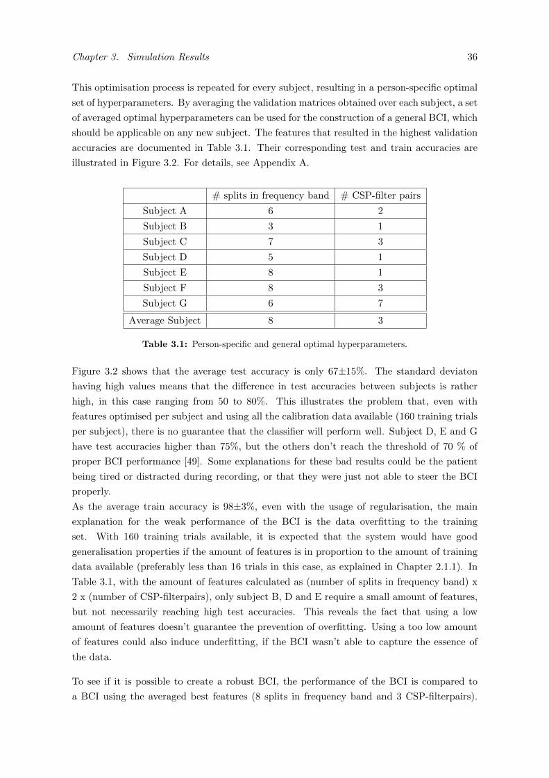
Chapter 3. Simulation Results 36
This optimisation process is repeated for every subject, resulting in a person-specific optimal
set of hyperparameters. By averaging the validation matrices obtained over each subject, a set
of averaged optimal hyperparameters can be used for the construction of a general BCI, which
should be applicable on any new subject. The features that resulted in the highest validation
accuracies are documented in Table 3.1. Their corresponding test and train accuracies are
illustrated in Figure 3.2. For details, see Appendix A.
# splits in frequency band # CSP-filter pairs
Subject A 6 2
Subject B 3 1
Subject C 7 3
Subject D 5 1
Subject E 8 1
Subject F 8 3
Subject G 6 7
Average Subject 8 3
Table 3.1: Person-specific and general optimal hyperparameters.
Figure 3.2 shows that the average test accuracy is only 67±15%. The standard deviaton
having high values means that the difference in test accuracies between subjects is rather
high, in this case ranging from 50 to 80%. This illustrates the problem that, even with
features optimised per subject and using all the calibration data available (160 training trials
per subject), there is no guarantee that the classifier will perform well. Subject D, E and G
have test accuracies higher than 75%, but the others don’t reach the threshold of 70 % of
proper BCI performance [49]. Some explanations for these bad results could be the patient
being tired or distracted during recording, or that they were just not able to steer the BCI
properly.
As the average train accuracy is 98±3%, even with the usage of regularisation, the main
explanation for the weak performance of the BCI is the data overfitting to the training
set. With 160 training trials available, it is expected that the system would have good
generalisation properties if the amount of features is in proportion to the amount of training
data available (preferably less than 16 trials in this case, as explained in Chapter 2.1.1). In
Table 3.1, with the amount of features calculated as (number of splits in frequency band) x
2 x (number of CSP-filterpairs), only subject B, D and E require a small amount of features,
but not necessarily reaching high test accuracies. This reveals the fact that using a low
amount of features doesn’t guarantee the prevention of overfitting. Using a too low amount
of features could also induce underfitting, if the BCI wasn’t able to capture the essence of
the data.
To see if it is possible to create a robust BCI, the performance of the BCI is compared to
a BCI using the averaged best features (8 splits in frequency band and 3 CSP-filterpairs).

Chapter 3. Simulation Results 37
A B C D E F G Average0
0.1
0.2
0.3
0.4
0.5
0.6
0.7
0.8
0.9
1
Test A
ccura
cy
Test Accuracy
Train Accuracy
Figure 3.2: The train and test accuracies reached when using the person-specific optimal features.
A second comparison is done with a BCI using only two splits in the frequency band and
3 CSP-filterpairs (see Figure 3.3). These splits are based on the alpha band (8-13 Hz) and
beta band (13-30 Hz), as these two frequency bands contain the most relevant information
for Motor Imagery applications. The delta (0-4 Hz) and gamma band (4-8 Hz) are left out
as literature has proven better performance when restricting the frequency range from 8 - 30
Hz [40] [39].
Figure 3.3 shows that the performance on the test set is not guaranteed to be highest when
the personal best features are used. This is due to the possible occurence of overfitting, as
the amount of features were optimised for the training data, and not for the testing data.
This can result in other combinations of features being better for the unseen test data.
Using only the alpha and beta band, the test accuracy is higher for every subject (except
for subject A) than when using the personal best features. This may be due to the proper
amount of features (= 2 x 2 bands x 3 CSP-filterpairs), avoiding overfitting and by only using
frequency bands that are medically relevant.
On average, the last method performs best, but with the standard deviations being high,
it is not possible to draw conclusions on which hyperparameters perform best. The only
conclusion that can be drawn is the high level of difficulty to construct a proper BCI model
for every subject.

Chapter 3. Simulation Results 38
A B C D E F G Average0
0.1
0.2
0.3
0.4
0.5
0.6
0.7
0.8
0.9
1
Test A
ccura
cy
Personal best
Averaged best
Alpha and Beta band
Figure 3.3: Comparison of the test accuracies when using person-specific optimised features, an
averaged optimal amount of features and when only using data from the alpha and beta
band.
3.2 Transfer Learning
With the problem of constructing highly performing BCI’s, illustrated in Figure 3.2 and
Figure 3.3, some Transfer Learning techniques will be tested to see if it is possible to reach
higher test accuracies, with less training data from the new subject.
In Transfer Learning, the data transferred between subjects doesn’t necessarily has to be
derived from the same task (e.g., left hand movement, right foot movement,...), but it has to
be similar.
In this work, only data from subjects that did perform the same tasks is used, as this gives
a first indication of the possibilities that Transfer Learning techniques hold. Therefore, from
here on, subject A and subject F will be left out as the imaginary movement of those subjects
were left hand and foot movement and the other majority of subjects chose left and right
hand movement.
Later on, this can be expanded to transferring data originating from different tasks.
For clarity of the graphs, in the upcoming figures, no error bars are shown when averaging
results over subjects, as the standard deviations can vary from 7 to 20%, with no relation
to the amount of calibration trials. By only comparing 5 subjects, the average can give an
indication of the performance of the methods, but for accurate comparisons, the investigation
has to be done subject-specific.

Chapter 3. Simulation Results 39
First, four Transfer Learning techniques from literature will be evaluated on our dataset.
These standard techniques are compared and explored further to build a new Transfer Learn-
ing technique that should reduce the calibration time as much as possible.
3.2.1 State of the art techniques
In the first comparison the four following techniques are used: Majority Voting, Averaging
Probabilities, Covariance Shrinkage and Data Space Adaption as explained in Chapter 2.7.
To see the influence of the amount of calibration trials on the performance of the classifier,
several experiments are done with the training set size ranging from 10 to 160 trials, in steps
of 10 trials. The test set will contain the last 40 trials.
Comparison between methods: 3 - 40 Hz
In Figure 3.4, results from five methods are compared: using no Transfer Learning, using
two naive Transfer Learning techniques, being Majority Voting and Averaging Probabilities
and using two Transfer Learning techniques from literature, being Covariance Shrinkage and
Data Space Adaption. Having data available from five source subjects, different experiments
are executed with a variable amount of calibration trials, ranging from 10 to 160 trials from
every source subject. Testing is done on the last 40 trials of the target subject. During
pre-processing (as in Chapter 3.1), the data is filtered from 3 - 40 Hz. The delta waves are
left out, as these occur during relaxation and sleep, not during Motor Imagery. According to
literature [47][48], no splitting in the frequency band is done. Concerning CSP-filtering, the
three most discriminative pairs of filters are used as features and given to a regularised LDA
classifier.
From Figure 3.4a, it is clear that DSA, on average, gives the best results, as the test accuracy
is highest for every amount of calibration data. Covariance Shrinkage, on average, doesn’t
always score better than when using no transfer learning. In some cases (see Figure 3.4f) it
does give higher performance, even close to the results obtained by DSA, but for the other
subjects, Covariance Shrinkage performs only a little better or the same in comparison to
when not applying Transfer Learning.
The sudden decrease in performance of Covariance Shrinkage for subject G when using 80, 90
and 100 calibration trials, may be due to a shift in the calibration data, causing the selection
of the best subset or the regularisation parameter (as in Formula 2.28) to change.
The Naive Transfer Learning techniques, being Majority Voting and Averaging Probabilities,
on average, give the same results being 53±5% and 3% respectively. When not much cal-
ibration data is available (<50 trials), for subject B, C and E, they score better than when
applying no Transfer Learning, but as the performance stays relatively low, independent of
the amount of calibration data, there is no future in these naive Transfer Learning techniques.

Chapter 3. Simulation Results 40
20 40 60 80 100 120 140 1600
0.2
0.4
0.6
0.8
1
Number of calibration trials
Te
st
Accu
racy
No Transfer Learning
Covariance Shrinkage
DSA
Majority Voting
Averaging Probabilities
(a) Average
20 40 60 80 100 120 140 1600
0.2
0.4
0.6
0.8
1
Number of calibration trials
Te
st
Accu
racy
No Transfer Learning
Covariance Shrinkage
DSA
Majority Voting
Averaging Probabilities
(b) Target subject B
20 40 60 80 100 120 140 1600
0.2
0.4
0.6
0.8
1
Number of calibration trials
Te
st
Accu
racy
No Transfer Learning
Covariance Shrinkage
DSA
Majority Voting
Averaging Probabilities
(c) Target subject C
20 40 60 80 100 120 140 1600
0.2
0.4
0.6
0.8
1
Number of calibration trials
Te
st
Accu
racy
No Transfer Learning
Covariance Shrinkage
DSA
Majority Voting
Averaging Probabilities
(d) Target subject D
20 40 60 80 100 120 140 1600
0.2
0.4
0.6
0.8
1
Number of calibration trials
Te
st
Accu
racy
No Transfer Learning
Covariance Shrinkage
DSA
Majority Voting
Averaging Probabilities
(e) Target subject E
20 40 60 80 100 120 140 1600
0.2
0.4
0.6
0.8
1
Number of calibration trials
Te
st
Accu
racy
No Transfer Learning
Covariance Shrinkage
DSA
Majority Voting
Averaging Probabilities
(f) Target subject G
Figure 3.4: Comparison of different Transfer Learning techniques, filtering from 3 - 40 Hz.

Chapter 3. Simulation Results 41
What is odd in these graphs is that the test accuracy for subject B, C and D, when not
applying Transfer Learning, does not increase with more calibration trials becoming available.
It might be that the range of 3 - 40 Hz is not optimal for Motor Imagery classification, so in
the next comparison a different frequency band is used.
Comparison between methods: 8 - 35 Hz
In Figure 3.5, the same comparison as in 3.2.1 is done, with the only difference the data
being filtered from 8 - 35 Hz, as this was the frequency range used in the papers describing
the method of Covariance Shrinkage and DSA. By only using the frequencies from 8 - 35 Hz,
alpha waves, beta waves and the beginning of gamma waves are measured. These include the
most import wave categories for Motor Imagery classification. [22]
On average, when comparing Figure 3.4a and Figure 3.5a, it seems like the performance of
DSA is lower when filtering from 8 - 35 Hz, but when looking subject-specific, the difference
in performance between this frequency range and when filtering from 3 - 40 Hz is not signi-
ficant when using less than 20 calibration trials (p>0.2).
What does decrease, is the robustness of DSA. For subject B and G, the DSA line shows
different peaks between certain amounts of calibration data. This is due to the altering in
covariance matrices when new training data becomes available, resulting in a different choice
of the best source subject. If hereafter, more calibration trials are added, the algorithm sta-
bilises back into their previous better working form and the right source subject is rechosen.
The performance of Covariance Shrinkage, on average, does increase significant when nar-
rowing down the frequency spectrum. On the other hand, when looking at subject B, C and
E, the Covariance Shrinkage line stays the same as when no Transfer Learning is used. Only
for subject B and G it can give higher test accuracies.
The performance of the BCI when not using Transfer Learning does look more logic in this
frequency range. It starts off with a low test accuracy and increases with more training data
becoming available.
The naive Transfer Learning techniques still show low performance, for the same reason as
in the other frequency range, as they don’t use properties of the calibration trials.
The high performance of DSA for the 3 - 40 Hz frequency band, may be due to the particular
choice of subjects in our dataset, but might not work as good in a more general system. As
the frequency range of 8 - 35 Hz is more related to Motor Imagery classification and gives
more logical results when not applying Transfer Learning, this range will be used for further
experiments.

Chapter 3. Simulation Results 42
20 40 60 80 100 120 140 1600
0.2
0.4
0.6
0.8
1
Number of calibration trials
Te
st
Accu
racy
No Transfer Learning
Covariance Shrinkage
DSA
Majority Voting
Averaging Probabilities
(a) Average
20 40 60 80 100 120 140 1600
0.2
0.4
0.6
0.8
1
Number of calibration trials
Te
st
Accu
racy
No Transfer Learning
Covariance Shrinkage
DSA
Majority Voting
Averaging Probabilities
(b) Target subject B
20 40 60 80 100 120 140 1600
0.2
0.4
0.6
0.8
1
Number of calibration trials
Te
st
Accu
racy
No Transfer Learning
Covariance Shrinkage
DSA
Majority Voting
Averaging Probabilities
(c) Target subject C
20 40 60 80 100 120 140 1600
0.2
0.4
0.6
0.8
1
Number of calibration trials
Te
st
Accu
racy
No Transfer Learning
Covariance Shrinkage
DSA
Majority Voting
Averaging Probabilities
(d) Target subject D
20 40 60 80 100 120 140 1600
0.2
0.4
0.6
0.8
1
Number of calibration trials
Te
st
Accu
racy
No Transfer Learning
Covariance Shrinkage
DSA
Majority Voting
Averaging Probabilities
(e) Target subject E
20 40 60 80 100 120 140 1600
0.2
0.4
0.6
0.8
1
Number of calibration trials
Te
st
Accu
racy
No Transfer Learning
Covariance Shrinkage
DSA
Majority Voting
Averaging Probabilities
(f) Target subject G
Figure 3.5: Comparison of different Transfer Learning techniques, filtering from 8 - 35 Hz.

Chapter 4
Design of a new Transfer Learning
method
In this chapter, a new Transfer Learning method is proposed to overcome the problem of
interperson and intersession differences, resulting in long calibration times. The new method
should reduce the calibration time, while maintaining a high level of performance.
By studying the results acquired in Chapter 3, a new Transfer Learning method is built by
combining or adapting the Transfer Learning methods from literature, in order to better
classify data from a new unseen subject.
To design this method, further investigation is done on the working principles of Covariance
Shrinkage (Chapter 2.7.2) and Data Space Adaption (Chapter 2.7.3).
4.1 Working principles of Covariance Shrinkage and Data Space
Adaption
In Covariance Shrinkage a Subject Selection Algorithm (see Section 2.7.2) is used, meaning
that not necessarily all the data of the previously recorded source subjects is used to construct
the covariance matrix in regularizing CSP and LDA. To see the effects of the Subject Selection
Algorithm, results were produced by using all source subjects, instead of selecting a subset
of source subjects. In the following graphs, this method is called ‘Covariance Shrinkage - No
subset’.
In Data Space Adaption, after having performed the Subject-to-Subject adaptation, there
is a selection of the best calibration model (see Section 2.7.3). To see what the effect of
this selection is, this selection is left out. Instead of choosing the best calibration model, all
models can now predict labels of new incoming trials and afterwards, the best calibration
model is chosen based on the highest test accuracy. This technique is not allowed in Machine
Learning algorithms, as it uses posterior information being the test accuracy, but here it
is only used for illustration purposes, to check whether the selection method of DSA works
43

Chapter 4. Design of a new Transfer Learning method 44
optimal. This method is called ‘DSA - Idealistic’ in the following graphs.
In Figure 4.1 five methods are plotted: No Transfer Learning as a baseline, Covariance
Shrinkage and DSA as previously plotted and the adapted versions of Covariance Shrinkage
and DSA.
Figure 4.1a shows that, on average, the idealistic version of DSA scores better, for every
amount of calibration trials. Looking at Figure 4.1b the problem with the sudden decrease
in performance when going from 10 to 20 trials, is solved by using the idealistic version. This
means that, by the addition of new calibration data, another source subject was chosen for
transfer of data, but not the one that resulted in the highest test accuracy. As, for subject
B, E and G, the idealistic DSA scores better or equal to the standard DSA, it is clear that
there is still room for improvement in the DSA algorithm, including removal of the stability
problem for subject B, E and G, as sudden drops in test accuracy are unwanted results.
When comparing the performance of Covariance Shrinkage with and without a selection of
subsets, from the average test accuracy in Figure 4.1a no conclusions can be drawn. When
looking at every subject individually, choosing all source subjects either works worse (as
in subject B), a little better (as in subject C until 60 trials), but for subject C (from 60
trials), D (from 40 trials) and E (from 30 trials), the choice of subset did not alter the
results, as the regularisation parameter (see Formula 2.28) stayed at zero, independent of the
subset of source subjects. A detailed comparison of the chosen subset and the corresponding
regularisation parameter with and without a selection of subsets can be found in Appendix
B.

Chapter 4. Design of a new Transfer Learning method 45
20 40 60 80 100 120 140 1600
0.2
0.4
0.6
0.8
1
Number of calibration trials
Te
st
Accu
racy
No Transfer Learning
Covariance Shrinkage
Covariance Shrinkage − No subset
DSA
DSA − Idealistic
(a) Average
20 40 60 80 100 120 140 1600
0.2
0.4
0.6
0.8
1
Number of calibration trials
Te
st
Accu
racy
No Transfer Learning
Covariance Shrinkage
Covariance Shrinkage − No subset
DSA
DSA − Idealistic
(b) Target subject B
20 40 60 80 100 120 140 1600
0.2
0.4
0.6
0.8
1
Number of calibration trials
Te
st
Accu
racy
No Transfer Learning
Covariance Shrinkage
Covariance Shrinkage − No subset
DSA
DSA − Idealistic
(c) Target subject C
20 40 60 80 100 120 140 1600
0.2
0.4
0.6
0.8
1
Number of calibration trials
Te
st
Accu
racy
No Transfer Learning
Covariance Shrinkage
Covariance Shrinkage − No subset
DSA
DSA − Idealistic
(d) Target subject D
20 40 60 80 100 120 140 1600
0.2
0.4
0.6
0.8
1
Number of calibration trials
Te
st
Accu
racy
No Transfer Learning
Covariance Shrinkage
Covariance Shrinkage − No subset
DSA
DSA − Idealistic
(e) Target subject E
20 40 60 80 100 120 140 1600
0.2
0.4
0.6
0.8
1
Number of calibration trials
Te
st
Accu
racy
No Transfer Learning
Covariance Shrinkage
Covariance Shrinkage − No subset
DSA
DSA − Idealistic
(f) Target subject G
Figure 4.1: Illustration of the working principles of Covariance Shrinkage and Data Space Adaption.

Chapter 4. Design of a new Transfer Learning method 46
4.2 Adaption of existing methods
Based on the comparisons done between different Transfer Learning techniques in Chapter
3.2.1 and 4.1, it is clear that none of these methods result in a classifier that always performs
best, for every subject. Therefore, it is interesting to investigate new possibilities that could
increase the performance of these techniques with as little calibration data as possible.
4.2.1 DSA/CS - Accumulate source subject data
The first idea is a combination of the two promising Transfer Learning methods, Data Space
Adaption and Covariance Shrinkage.
• With the Subject-Selection Algorithm from Covariance Shrinkage, define the best sub-
set.
• Place the trials of these subjects after each other, as if the data would come from one
target.
• Transform the calibration data of the target subject according to the transformation
matrix M (as calculated in Formula 2.29), using the covariance matrices of the accu-
mulated source subject data.
• Train the classifier with the accumulated source subject data and test it on the trans-
formed new trials.
4.2.2 DSA - Averaging probabilities (AP)
For the second idea a variant of Data Space Adaption is used.
• As in DSA, the calibration trials are transformed with a transformation matrix Mk,
based on the covariance matrices of each source subject k.
• Instead of selecting one best calibration model, multiple calibration models are selected,
by picking the ones that give the highest validation accuracies.
• As different classifiers are constructed based on different source subjects, for each trial,
the classifiers will output probabilities that are averaged.
By averaging the probabilities over the remaining classifiers, the drawback from the original
DSA algorithm, where new calibration data could induce a different choice of best source
subject, could be reduced, by averaging influences of multiple classifiers.
The choice for averaging the probabilities instead of using Majority Voting, is based on the
fact that by averaging probabilities, the effect of insecure classifiers is reduced. If three
insecure classifiers would predict a left-hand trial, and a fourth confident classifier would

Chapter 4. Design of a new Transfer Learning method 47
predict a right-hand trial, Majority Voting would result in a left-hand trial, while Averaging
Probabilities would result in a right-hand trial.
It was visible during the experiments, that almost always every source subject was chosen
based on validation accuracy, therefore this pre-selection of subjects is left out, resulting in
a method that averages the outputs of all classifiers.
4.2.3 DSA - Maximum probability (MP)
The third idea works according to the same principle as DSA - Averaging probabilities, but
instead of averaging the probabilities of the different classifiers, the trial will be classified
according to the class to which the highest probability was given by a classifier. As for
DSA - AP, there will be no pre-selection of subjects based on validation accuracy.
4.2.4 Comparison
In Figure 4.2 and Figure 4.3these ideas are compared to the existing methods for every source
subject. The new methods are plotted with solid lines, the old techniques from literature are
plotted in dashed lines. As the focus of the new Transfer Learning technique lies on using
as little calibration data as possible, these experiments are performed with a training set
size varying from 2 to 30 calibration trials, in steps of 2 trials, after which experiments are
performed in steps of 10 trials in training set size. To be able to see the small differences
between test accuracies, only the range from 50% to 100% is plotted.
From Figure 4.2 it is clear that no new method can be identified as the best performing
method for every target, neither based on the average performance, neither on individual
performance of the methods.
As our goal is to reduce calibration time, the aim of the new method should be to give high
test accuracies with a low amount of calibration data, hence the focus of the comparison is
on the left part of the graphs in Figure 4.2. A more detailed view on the experiments done
using two to 40 calibration trials is shown in Figure 4.3.
For subject B and subject D, DSA - AP and DSA - MP don’t give the best results, but
at least the test accuracies remain stable with few calibration data, in comparison to the
performance of DSA/CS and DSA.
For subject C and subject G, DSA - AP and DSA - MP do give the best overall results, so
in these cases, the first idea is discarded.
For subject E, the best method depends on the number of calibration trials, with test ac-
curacies for all methods fluctuating when few calibration data is given. This may be due to
the first consecutive trials of subject E being indecisive or unclear to the BCI.

Chapter 4. Design of a new Transfer Learning method 48
20 40 60 80 100 120 140 1600.5
0.6
0.7
0.8
0.9
1
Number of calibration trials
Te
st
Accu
racy
No Transfer Learning
DSA
DSA / CS
DSA − AP
DSA − MP
(a) Average
20 40 60 80 100 120 140 1600.5
0.6
0.7
0.8
0.9
1
Number of calibration trials
Te
st
Accu
racy
No Transfer Learning
DSA
DSA / CS
DSA − AP
DSA − MP
(b) Target subject B
20 40 60 80 100 120 140 1600.5
0.6
0.7
0.8
0.9
1
Number of calibration trials
Te
st
Accu
racy
No Transfer Learning
DSA
DSA / CS
DSA − AP
DSA − MP
(c) Target subject C
20 40 60 80 100 120 140 1600.5
0.6
0.7
0.8
0.9
1
Number of calibration trials
Te
st
Accu
racy
No Transfer Learning
DSA
DSA / CS
DSA − AP
DSA − MP
(d) Target subject D
20 40 60 80 100 120 140 1600.5
0.6
0.7
0.8
0.9
1
Number of calibration trials
Te
st
Accu
racy
No Transfer Learning
DSA
DSA / CS
DSA − AP
DSA − MP
(e) Target subject E
20 40 60 80 100 120 140 1600.5
0.6
0.7
0.8
0.9
1
Number of calibration trials
Te
st
Accu
racy
No Transfer Learning
DSA
DSA / CS
DSA − AP
DSA − MP
(f) Target subject G
Figure 4.2: Comparison of No Transfer Learning, DSA and three new methods.

Chapter 4. Design of a new Transfer Learning method 49
5 10 15 20 25 30 35 400.5
0.6
0.7
0.8
0.9
1
Number of calibration trials
Te
st
Accu
racy
No Transfer Learning
DSA
DSA / CS
DSA − AP
DSA − MP
(a) Average
5 10 15 20 25 30 35 400.5
0.6
0.7
0.8
0.9
1
Number of calibration trials
Te
st
Accu
racy
No Transfer Learning
DSA
DSA / CS
DSA − AP
DSA − MP
(b) Target subject B
5 10 15 20 25 30 35 400.5
0.6
0.7
0.8
0.9
1
Number of calibration trials
Te
st
Accu
racy
No Transfer Learning
DSA
DSA / CS
DSA − AP
DSA − MP
(c) Target subject C
5 10 15 20 25 30 35 400.5
0.6
0.7
0.8
0.9
1
Number of calibration trials
Te
st
Accu
racy
No Transfer Learning
DSA
DSA / CS
DSA − AP
DSA − MP
(d) Target subject D
5 10 15 20 25 30 35 400.5
0.6
0.7
0.8
0.9
1
Number of calibration trials
Te
st
Accu
racy
No Transfer Learning
DSA
DSA / CS
DSA − AP
DSA − MP
(e) Target subject E
5 10 15 20 25 30 35 400.5
0.6
0.7
0.8
0.9
1
Number of calibration trials
Te
st
Accu
racy
No Transfer Learning
DSA
DSA / CS
DSA − AP
DSA − MP
(f) Target subject G
Figure 4.3: Comparison of No Transfer Learning, DSA and three new methods, focusing on the
experiments done with 40 calibration trials or less.

Chapter 4. Design of a new Transfer Learning method 50
Using a dependent t-test, it can be measured whether the test accuracies across 5 subjects
differ significantly when using one method or the other. In Figure 4.4, the performance of DSA
is compared to DSA-AP and DSA-MP respectively. It is seen that the p-value for both null-
hypothesis (H0 (DSA = DSA-MP) andH0 (DSA = DSA-AP)), for every amount of calibration
trials used, is always bigger than p = 0.05, so the null-hypothesis is not rejected. Only using
2 calibration trials, the null-hypothesis can be rejected with a p-value of respectively 0.02
and 0.03.
20 40 60 80 100 120 140 1600
0.1
0.2
0.3
0.4
0.5
0.6
0.7
0.8
0.9
1
Number of calibration trials
p−
valu
e
DSA / DSA−AP
DSA / DSA−MP
Figure 4.4: P-values for both null-hypothesis H0 (DSA = DSA-MP) and H0 (DSA = DSA-AP),
showing that the null-hypothesis can not be rejected.

Chapter 4. Design of a new Transfer Learning method 51
4.3 New Transfer Learning Technique
Based on the comparisons made in Figure 4.2, a new method is constructed. As neither DSA
- AP or DSA - MP reached significantly better results than DSA (see Figure 4.4), the new
method will combine the approaches of DSA - AP and DSA - MP.
This choice of methods relies on the fact that, depending on the amount of calibration data,
one of these three methods will give the highest test accuracy, as was illustrated in Figure 4.2.
To guarantee that the highest test accuracy is always reached, a new method is constructed
that should result in an upper boundary of DSA, DSA - AP and DSA - MP.
To be able to meet these conditions, further investigation is done on where DSA - AP and
DSA - MP make mistakes in classifying trials.
If DSA - AP is used, which averages the probabilities of the classifiers for every class, trials
are classified wrong if the decision is made based on a majority of classifiers, which are unsure
of their decision, prevailing the classifier that is sure of his decision to dominate. An example
can be seen in Table 4.1.
Table 4.1: Example of a possible outcome when predicting the class label for a trial of target subject
B, which should be a right-hand trial. When averaging the probabilities, the class label is
left, while when using the maximum of the probabilities the class label would be correctly
predicted as right.
P(Left) P(Right) Average(Left) Average(Right)
Source subject C 0.65 0.35 0.525 0.475
Source subject D 0.65 0.35 Maximum(Left) Maximum(Right)
Source subject E 0.6 0.40.65 0.8
Source subject G 0.2 0.8
This gives rise to a first criterion that the new method should remove or ignore the outcomes
of an unsure classifier.
If DSA - MP is used, which classifies based on the classifier that gives the highest probab-
ility, trials are classified wrong if one of the classifiers gives a very high probability, but the
other ones were right, with respectively a lower probability, illustrated in Table 4.2. This
brings to mind that even though accuracies are high, this doesn’t mean that they correctly
predict a class label. The new method should thus be able to detect classifiers that give high
probabilities, but don’t result in high performance.
Based on these findings, it is clear that DSA - AP and DSA - MP are complementary, but a
criterion has to be found whether to use the one or the other.

Chapter 4. Design of a new Transfer Learning method 52
Table 4.2: Example of a possible outcome when predicting the class label for a trial of target subject
B, which should be a left-hand trial. When taking the maximum of the probabilities, the
decision is a right-hand trial, while the majority of predictions is a left-hand trial.
P(Left) P(Right) Average(Left) Average(Right)
Source subject C 0.1 0.9 0.625 0.375
Source subject D 0.8 0.2 Maximum(Left) Maximum(Right)
Source subject E 0.8 0.20.8 0.9
Source subject G 0.8 0.2
In Algorithm 1, the set-up of the new Transfer Learning technique is described. Dependant
on whether a classifier is biased or if it’s validation accuracy is low, the source subject is
removed from the decision making process. These two specifications will be explained later.
The following variables and methods are used in Algorithm 1:
• Dc: training data from the target subject.
• Dt: new test data from the target subject.
• Dk, k ∈ 0, ..., Ns: previously recorded data from the source subjects, with Ns the
total amount of source subjects.
• CalculateM(X,Y) constructs the transformation matrix MY using the estimated covari-
ance matrices of subject X and Y to minimize their distribution differences, according
to Formula 2.29.
• ApplySource(X,Y, MY ) will calculate the validation accuracies when transforming the
data of subject Y, using MY to minimize the distribution differences between subject
X and Y.
The threshold of 70% for validation accuracies was chosen by comparing results when varying
this parameter from 60 to 90% in steps of 5%.
A classifier is labeled as biased if its predictions are consistently the same. How a classifier
is determined to be biased is illustrated with an example in Figure 4.5.
In this figure, 20 calibration trials of subject B are available. To see whether classifier C is a
biased classifier, data of other source subjects is used.
In step 1, data of the subsequent source subjects are adapted towards the available calibration
data, here D’, E’ and G’. In this way, more data is constructed with the same distribution as
target subject B.
In step 2, the testing of the BCI is mimiced by transforming D’, E’ and G’ (to minimise
distribution differences with subject C) towards D”, E” and G”, on which the BCI is tested
in step 3, after training on the 200 trials of source subject C.

Chapter 4. Design of a new Transfer Learning method 53
Algorithm 1 New Transfer Learning technique
Determine the transformation matrices and validation accuracies using the
calibration data Dc
BiasedClassifier() . Will set FlagBiased = True when biased
while k ≤ Ns do
Mk = CalculateM(Dc, Dk)
ValAcc = ApplySource(Dc, Dk,Mk)
if ValAcc ≤ 0.7 then
FlagV alidation(k) = True
end if
end while
Determine which source subjects of Dk should be left out, and whether the
probabilities should be averaged (standard) or use the maximum probability
of the remaining source subjects (if maxProb = True).
if (# FlagV alidation == True) ≥ Ns/2 then
if (# FlagBiased == True) <Ns/2 then
Remove the biased source subject from Ds
end if
maxProb = True
else
Remove the source subject with FlagV alidation = True
if (# FlagBiased == True) <Ns/2 then
Remove the biased source subject from Ds
else
maxProb = True
end if
end if
Determine the test accuracy with Dt
while k ≤ Ns do
Probabilities(k) = ApplySource(Dt, Dk,Mk)
end while
if maxProb == True then
Use the maximum probability of Probabilities(k)
else
Average the probabilities of Probabilities(k)
end if

Chapter 4. Design of a new Transfer Learning method 54
The BCI is trained according to the same principles as for DSA, using the same amount of
calibration trials from respectively D, E and G, with subject C serving as the source subject.
For testing, 40 trials are used. If, for more than half of the temporary classifiers, more than
90% of the trials are labeled the same, the source subject C is flagged as biased.
This threshold of 90% was chosen by comparing results when varying this parameter from
70 to 95% in steps of 5%.
Target subject: B Classifier to be checked if biased:Source subject CNumber of calibration trials: 20 Other source subjects: Subject D, E and G
Construct transformation
matrices
MDàB
MEàB
MGàB
Transform
D à D’
E à E’
G à G’
Construct transformation
matrices
MD’àC
ME’àC
MG’àC
Transform
D’ à D’’
E’ à E’’
G’ à G’’
Train
C
Test
D’’
E’’
G’’
1 2 3
Figure 4.5: From target subject B, 20 calibration trials are available. For the transformation between
target subject B and the source subjects in step 1 and the transformation in step 2, the
same amount of trials from the source subjects are used.

Chapter 5
Experimental Results
The results of the new Transfer Learning technique are plotted in Figure 5.1. The new
method is indicated with a red solid line.
Based on Figure 5.1a, the new method could be labeled as the best performing one, but when
looking subject-specific, the results vary.
For subject C and subject G, the new Transfer Learning technique scores best for every
amount of calibration data. For subject G, there is a slight decrease in performance for 6
calibration trials, but the performance is not as dependant on the amount of calibration trials
as in DSA.
For subject B, the new method’s accuracy mostly stays below the one of DSA, but at least
it doesn’t suddenly drop to accuracies below 60%.
For subject D, the results are not optimal with few calibration data. One can see that the
accuracies for the new method stay above 80%, but the variation from 2 to 20 calibration
trials is high. This may be due to the discrimination based on low validation accuracies or
biased classifiers, not being able to point the best source subject/subjects to use, as DSA
sometimes results in higher accuracies up until 50 calibration trials.
For subject E, the same conclusion can be made with regards to the performance of DSA,
with the difference of the new method being more stable than DSA (except for the peak in
the beginning).
In Figure 5.2, the same results are shown, but only the experiments using 40 calibration trials
or less, and focusing on the range of test accuracies above 50%. The numeric results can be
found in Appendix C.
55

Chapter 5. Experimental Results 56
20 40 60 80 100 120 140 1600
0.2
0.4
0.6
0.8
1
Number of calibration trials
Te
st
Accu
racy
No Transfer Learning
DSAMajority Voting
New TL technique
(a) Average
20 40 60 80 100 120 140 1600
0.2
0.4
0.6
0.8
1
Number of calibration trials
Te
st
Accu
racy
No Transfer Learning
DSAMajority Voting
New TL technique
(b) Target subject B
20 40 60 80 100 120 140 1600
0.2
0.4
0.6
0.8
1
Number of calibration trials
Te
st
Accu
racy
No Transfer Learning
DSAMajority Voting
New TL technique
(c) Target subject C
20 40 60 80 100 120 140 1600
0.2
0.4
0.6
0.8
1
Number of calibration trials
Te
st
Accu
racy
No Transfer Learning
DSAMajority Voting
New TL technique
(d) Target subject D
20 40 60 80 100 120 140 1600
0.2
0.4
0.6
0.8
1
Number of calibration trials
Te
st
Accu
racy
No Transfer Learning
DSAMajority Voting
New TL technique
(e) Target subject E
20 40 60 80 100 120 140 1600
0.2
0.4
0.6
0.8
1
Number of calibration trials
Te
st
Accu
racy
No Transfer Learning
DSAMajority Voting
New TL technique
(f) Target subject G
Figure 5.1: Comparison of No Transfer Learning, Majority Voting, DSA and the new Transfer Learn-
ing technique.

Chapter 5. Experimental Results 57
5 10 15 20 25 30 35 400.5
0.6
0.7
0.8
0.9
1
Number of calibration trials
Te
st
Accu
racy
No Transfer Learning
DSA
Majority Voting
New TL technique
(a) Average
5 10 15 20 25 30 35 400.5
0.6
0.7
0.8
0.9
1
Number of calibration trials
Te
st
Accu
racy
No Transfer Learning
DSA
Majority Voting
New TL technique
(b) Target subject B
5 10 15 20 25 30 35 400.5
0.6
0.7
0.8
0.9
1
Number of calibration trials
Te
st
Accu
racy
No Transfer Learning
DSA
Majority Voting
New TL technique
(c) Target subject C
5 10 15 20 25 30 35 400.5
0.6
0.7
0.8
0.9
1
Number of calibration trials
Te
st
Accu
racy
No Transfer Learning
DSA
Majority Voting
New TL technique
(d) Target subject D
5 10 15 20 25 30 35 400.5
0.6
0.7
0.8
0.9
1
Number of calibration trials
Te
st
Accu
racy
No Transfer Learning
DSA
Majority Voting
New TL technique
(e) Target subject E
5 10 15 20 25 30 35 400.5
0.6
0.7
0.8
0.9
1
Number of calibration trials
Te
st
Accu
racy
No Transfer Learning
DSA
Majority Voting
New TL technique
(f) Target subject G
Figure 5.2: Comparison of No Transfer Learning, Majority Voting, DSA and the new Transfer Learn-
ing technique, focused on the experiments done with 40 calibration trials or less.

Chapter 6
Conclusion and future work
By using Brain-Computer Interfaces, people who have lost the ability to control their limbs
are given the opportunity to steer an application using Motor Imagery, but due to interperson
and intersession differences, the BCI needs to adapt to the new user’s brain to be able to
correctly classify their thoughts, for every use of the application. This calibration could take
up to 20 - 30 minutes, giving a lot of room for improvement.
The difficulty of constructing a good BCI was proven by the low testing accuracies that were
reached when constructing a person-specific BCI, even though sufficient training data was
available. As for some targets the testing accuracy didn’t even reach 70%, but for some users
the BCI could reach 90% performance, the system is clearly user-dependent.
Averaging the optimal settings of the person-specific BCI’s resulted in higher accuracies for
some targets, but on average, no significant difference was noted (p=0.45). Averaging optimal
settings when only using frequency bands common in Motor Imagery classification (the alpha
and beta band), could also lead to higher accuracies for some targets, but with these results
not scoring significantly worse (p=0.33), it is an indication for further use of this frequency
band only.
These first experiments gave rise to two problems: the system being very user-dependent
and the need for a lot of calibration data. These findings dictate the fact that advanced
techniques will be needed to guarantee a good performance of the BCI, independent of the
user performing the Motor Imagery task and preferably with as little calibration data as
possible.
In this attempt, several experiments were done using different Transfer Learning techniques.
By comparing different Transfer Learning techniques, varying from naive methods as aver-
aging probabilities and majority voting, to methods that transform the test data according
to covariance matrices, it became clear that none of these methods could be labeled as the
one that would always result in the highest performance. When getting to the bottom of the
techniques that performed significantly better than when not using Transfer Learning at all,
the need for improvement of DSA arose.
58

Chapter 6. Conclusion and future work 59
This shortcoming of DSA was the baseline for the construction of a new method. The main
problem of the current Transfer Learning techniques is finding the best subject from which
information can be transferred, or in some cases, the best subjects. In the case of multiple
subjects being a good fit for the job, the outputs of the classifiers could either be averaged
or the maximum could be taken. Experimenting with these ideas, showed that neither one
of these approaches induces the highest possible performance for every amount of calibration
data. Where one method performs bad, the other one will perform well.
These findings led to a new Transfer Learning technique that combined both averaging the
outputs of different classifiers and taking the maximum probability produced by a classifier.
The amount of classifiers on which Transfer Learning is applied and the preferred method
used, is based on a selection criterion.
The strength of this new Transfer Learning technique is its robustness in comparison to
DSA. Where the performance of DSA suddenly decreases when new calibration data becomes
available, the new method is less sensitive to alterations in calibration data. With regards
to an application of a BCI to steer a wheelchair, this advantage of the new method is an
important aspect in sending the wheelchair towards the right direction, even if the user was
confused or distracted for a short period of time. The new method might not always be
stated as the best method for every amount of calibration data, but by further alterations in
the selection criterion, the results can be promising.
At the moment, as seen in Figure 5.1, with a single exception for 6 calibration trials when
testing for target E, the test accuracy of the new Transfer Learning technique, never drops
below 67%. The most important gain in performance is that, when only having 4 calibration
trials available, the test accuracy is minimally 77%. With respect to, when having 4 calibra-
tion trials available, only reaching 52±6% on average when not applying Transfer Learning.
In the worst case scenario, there is even an improvement of 38%. On average, when using the
final method and 4 calibration trials, the test accuracy is 86±8%. This clearly manifests that,
by applying Transfer Learning and reducing the amount of calibration, there was absolutely
no reduction in performance.
With regards to the goal of reducing the calibration time as much as possible, this requirement
is fullfilled, as the amount of trials is reduced to the minimal amount of trials possible (one
trial of each class), still reaching average test accuracies of 85±10%.
In the construction of a new method, based on comparisons between old and new techniques,
it might not be overlooked that an optimal method was constructed based on data from only
5 subjects. To work around this restriction, the steps taken in the process to construct a
new Transfer Learning technique were not based on the averages of the performance of these
5 subjects, but on target-specific results. As these results still might depend on the specific
data used in the experiments, it might be useful to go over the same steps and reasonings,
but with a larger or a different dataset.

Chapter 6. Conclusion and future work 60
Another path that can be explored is by adding more Motor Imagery tasks to the classification
problem, to study the generalisation properties of the Transfer Learning method. For the
application of steering a wheelchair, this could be the addition of a stop and backwards
command. The removal of restricting the BCI to be synchronous would also be a big step in
the right direction, as it gives the possibility to the user to communicate at their own pace.
But before exploiting these options, further thought should be given on how to eliminate the
calibration procedure and making it an online application that learns from the user, while
already performing the first movements, preferably in the right direction.

Appendix A
Hyperparameters for a first BCI
To determine the best set of hyperparameters, the validation matrices are averaged over all
subjects. This resulted in the validation matrix as in Table A.1. The rows indicate how much
splits in the frequency band are used, the columns indicate the amount of CSP-filters used.
These validation accuracies are averages, so the low average validation accuracies are due to
some subjects for whom it is hard to construct a proper BCI (like for subject B, who never
results in validation accuracies higher than 0.543). On the other hand, subjects like D and
G, easily reach validation accuracies of 0.8 or higher.
On average, according to a validation accuracy of 0.693, the best hyperparameters are ob-
tained, as highlighted, when splitting the frequency band in 8 equal splits and using 3 CSP
filter pairs.
1 2 3 4 5 6 7 8 9
0 0.467 0.477 0.472 0.485 0.478 0.489 0.489 0.489 0.487
1 0.515 0.514 0.541 0.563 0.555 0.549 0.537 0.540 0.546
2 0.564 0.587 0.576 0.593 0.581 0.568 0.55 0.542 0.559
3 0.618 0.631 0.634 0.635 0.621 0.615 0.603 0.602 0.615
4 0.604 0.667 0.645 0.645 0.641 0.622 0.646 0.632 0.610
5 0.637 0.644 0.652 0.642 0.620 0.629 0.614 0.610 0.622
6 0.662 0.678 0.683 0.668 0.652 0.647 0.645 0.640 0.636
7 0.654 0.680 0.682 0.6625 0.651 0.65 0.635 0.632 0.630
8 0.657 0.692 0.693 0.651 0.649 0.656 0.634 0.622 0.629
9 0.655 0.690 0.685 0.647 0.647 0.657 0.637 0.630 0.622
Table A.1: Validation accuracies averaged over all source subjects. The rows indicate how much
splits in the frequencyband are used, the columns indicate the amount of CSP-filters
used.
The test and train accuracies reached with person-specific optimal features are seen in Table
A.2. The test accuracies obtained when using person-specific optimal features, averaged
optimal features and when using only the alpha and beta band are seen in Table A.3.
61

Appendix A. Hyperparameters for a first BCI 62
Test Accuracy Train Accuracy
Subject A 0.500 0.969
Subject B 0.525 0.925
Subject C 0.600 1.000
Subject D 0.775 0.975
Subject E 0.900 0.994
Subject F 0.575 0.988
Subject G 0.800 1.000
Average 0.668 ± 0.217 0.979 ± 0.318
Table A.2: Train and test accuracies reached when using the person-specific optimal features.
Personal best Averaged best Alpha and Beta band
Subject A 0.500 0.675 0.475
Subject B 0.525 0.575 0.600
Subject C 0.600 0.575 0.750
Subject D 0.775 0.950 0.800
Subject E 0.900 0.850 0.950
Subject F 0.575 0.575 0.600
Subject G 0.800 0.700 0.800
Average 0.668 ± 0.217 0.700 ± 0.224 0.711 ± 0.230
Table A.3: Comparison of the test accuracies when using person-specific optimised features, an
averaged optimal amount of features and when only using data from the alpha and
beta band.

Appendix B
Covariance Shrinkage: Subset
selection and regularisation
parameter
The subset that was chosen by the Subject Selection Algorithm as in Chapter 2.7.2, is il-
lustrated in Table B.1. In the columns, the source subjects chosen for the corresponding
target subject in the header are shown. The corresponding regularisation parameter for each
experiment is added in Table B.2. In both tables, each row represents a new experiment
using a bigger amount of calibration trials.
In this table, the regularisation parameter when using the complete set of source subjects is
added for comparison. It is clear that there is no big difference in regularisation parameter
when a different subset is used. For subject C, D and E, the regularisation parameter is
mostly zero, so an altering in subset can not have an influence on the test accuracy. If the
regularisation parameter is non-zero, the subset chosen by the Subject Selection Algorithm
is nearly always a set of three out of four subjects, and as visible in Figure 4.1, for target
subject B, the addition of a fourth source subject lowers the test accuracy, where for target
subject G, the test accuracy slightly increases when adding a fourth source subject.
63

Appendix B. Covariance Shrinkage: Subset selection and regularisation parameter 64
Subject B Subject C Subject D Subject E Subject G
10 C G B, C D, G C, D, E
20 D, E, G B, C B, C, D, E
30 D, E, G B, C, D, E
40 D, E, G D, E, G B, C, D, E
50 D, E, G D, E, G C, D, E
60 D, E, G C, D, E
70 C, D, E C, D, E
80 C, D, E C, D, E
90 C, D, E C, D, E
100 C, D, E C, D, E
110 C, D, E C, D, E
120 C, D, E C, D, E
130 C, D, E C, D, E
140 C, D, E C, D, E
150 C, D, E C, D, E
160 C, D, E C, D, E
Table B.1: The subset of source subjects as chosen by the Subject Selection Algorithm (see Chapter
2.7.2).

Appendix B. Covariance Shrinkage: Subset selection and regularisation parameter 65
Subject B Subject C Subject D Subject E Subject G
S NS S NS S NS S NS S NS
10 1.000 0.167 1.000 1.000 1.000 1.000 1.000 1.000 1.000 0.778
20 0.000 0.000 1.000 1.000 0.000 1.000 0.143 1.000 1.000 0.769
30 1.000 1.000 0.000 0.000 0.000 1.000 0.000 0.000 1.000 1.000
40 1.000 1.000 0.087 1.000 0.000 0.000 0.000 0.000 1.000 1.000
50 1.000 1.000 1.000 1.000 0.000 0.000 0.000 0.000 0.667 0.615
60 1.000 1.000 0.000 0.000 0.000 0.000 0.000 0.000 1.000 0.606
70 1.000 1.000 0.000 0.000 0.000 0.000 0.000 0.000 0.324 0.308
80 1.000 1.000 0.000 0.000 0.000 0.000 0.000 0.000 0.529 0.486
90 1.000 1.000 0.000 0.000 0.000 0.000 0.000 0.000 0.458 0.500
100 1.000 1.000 0.000 0.000 0.000 0.000 0.000 0.000 0.407 0.407
110 1.000 1.000 0.000 0.000 0.000 0.000 0.000 0.000 0.321 0.367
120 1.000 1.000 0.000 0.000 0.000 0.000 0.000 0.000 0.222 0.364
130 0.132 0.134 0.000 0.000 0.000 0.000 0.000 0.000 0.093 0.104
140 0.029 1.000 0.000 0.000 0.000 0.000 0.000 0.000 0.061 0.059
150 0.012 0.013 0.000 0.000 0.000 0.000 0.000 0.000 0.048 0.050
160 0.057 0.054 0.000 0.000 0.000 0.000 0.000 0.000 0.026 0.025
Table B.2: The regularisation parameter when a subset of source subjects is chosen (S) and when
all subjects are chosen as source subjects (NS).

Appendix C
Results of the comparison of No
Transfer Learning, Majority Voting,
DSA and the new method
No Transfer Learning DSA Majority Voting New TL technique
2 0.520 0.670 0.520 0.845
4 0.520 0.760 0.520 0.860
6 0.475 0.725 0.520 0.765
8 0.470 0.760 0.520 0.870
10 0.450 0.735 0.520 0.815
12 0.480 0.795 0.520 0.845
14 0.450 0.810 0.520 0.820
16 0.430 0.730 0.520 0.825
18 0.470 0.715 0.520 0.835
20 0.510 0.735 0.520 0.845
22 0.510 0.785 0.520 0.865
24 0.535 0.810 0.520 0.865
26 0.530 0.805 0.520 0.865
28 0.530 0.835 0.520 0.865
30 0.495 0.825 0.520 0.870
40 0.565 0.800 0.520 0.865
Table C.1: Results of a comparison of different Machine Learning techniques, averaged over 5 target
subjects.
66

Appendix C. Results of the comparison of No Transfer Learning, Majority Voting, DSAand the new method 67
No Transfer Learning DSA Majority Voting New TL technique
2 0.425 0.750 0.550 0.800
4 0.425 0.825 0.550 0.775
6 0.550 0.750 0.550 0.775
8 0.525 0.850 0.550 0.700
10 0.500 0.875 0.550 0.675
12 0.525 0.925 0.550 0.700
14 0.525 0.925 0.550 0.700
16 0.575 0.500 0.550 0.700
18 0.475 0.525 0.550 0.725
20 0.500 0.525 0.550 0.725
22 0.500 0.825 0.550 0.725
24 0.475 0.825 0.550 0.750
26 0.450 0.850 0.550 0.750
28 0.500 0.850 0.550 0.775
30 0.525 0.675 0.550 0.800
40 0.500 0.925 0.550 0.800
Table C.2: Results of a comparison of different Machine Learning techniques, using subject B as
target subject.
No Transfer Learning DSA Majority Voting New TL technique
2 0.575 0.600 0.525 0.700
4 0.575 0.625 0.525 0.775
6 0.525 0.600 0.525 0.775
8 0.525 0.600 0.525 0.775
10 0.475 0.625 0.525 0.775
12 0.425 0.625 0.525 0.750
14 0.325 0.625 0.525 0.750
16 0.250 0.625 0.525 0.775
18 0.400 0.625 0.525 0.775
20 0.425 0.675 0.525 0.775
22 0.475 0.675 0.525 0.775
24 0.475 0.675 0.525 0.775
26 0.475 0.675 0.525 0.775
28 0.400 0.650 0.525 0.775
30 0.450 0.675 0.525 0.775
40 0.500 0.650 0.525 0.775
Table C.3: Results of a comparison of different Machine Learning techniques, using subject C as
target subject.

Appendix C. Results of the comparison of No Transfer Learning, Majority Voting, DSAand the new method 68
No Transfer Learning DSA Majority Voting New TL technique
2 0.550 0.725 0.500 0.850
4 0.550 0.825 0.500 0.875
6 0.450 0.875 0.500 0.925
8 0.475 0.825 0.500 0.950
10 0.550 0.900 0.500 0.800
12 0.600 0.825 0.500 0.925
14 0.525 0.900 0.500 0.800
16 0.475 0.900 0.500 0.850
18 0.525 0.925 0.500 0.850
20 0.625 0.925 0.500 0.850
22 0.600 0.850 0.500 0.875
24 0.675 0.925 0.500 0.875
26 0.600 0.850 0.500 0.850
28 0.575 0.850 0.500 0.875
30 0.575 0.950 0.500 0.875
40 0.650 0.950 0.500 0.900
Table C.4: Results of a comparison of different Machine Learning techniques, using subject D as
target subject.
No Transfer Learning DSA Majority Voting New TL technique
2 0.500 0.675 0.450 0.950
4 0.500 0.925 0.450 0.925
6 0.425 0.800 0.450 0.550
8 0.450 0.925 0.450 0.950
10 0.300 0.675 0.450 0.850
12 0.425 1.000 0.450 0.875
14 0.475 1.000 0.450 0.875
16 0.425 1.000 0.450 0.850
18 0.450 0.900 0.450 0.875
20 0.500 0.900 0.450 0.925
22 0.500 0.875 0.450 1.000
24 0.575 0.875 0.450 0.975
26 0.575 0.950 0.450 1.000
28 0.650 0.925 0.450 0.975
30 0.425 0.925 0.450 0.950
40 0.700 0.950 0.450 0.925
Table C.5: Results of a comparison of different Machine Learning techniques, using subject E as
target subject.

Appendix C. Results of the comparison of No Transfer Learning, Majority Voting, DSAand the new method 69
No Transfer Learning DSA Majority Voting New TL technique
2 0.550 0.600 0.575 0.925
4 0.550 0.600 0.575 0.950
6 0.425 0.600 0.575 0.800
8 0.375 0.600 0.575 0.975
10 0.425 0.600 0.575 0.975
12 0.425 0.600 0.575 0.975
14 0.400 0.600 0.575 0.975
16 0.425 0.625 0.575 0.950
18 0.500 0.600 0.575 0.950
20 0.500 0.650 0.575 0.950
22 0.475 0.700 0.575 0.950
24 0.475 0.750 0.575 0.950
26 0.550 0.700 0.575 0.950
28 0.525 0.900 0.575 0.925
30 0.500 0.900 0.575 0.950
40 0.475 0.525 0.575 0.925
Table C.6: Results of a comparison of different Machine Learning techniques, using subject G as
target subject.

Bibliography
[1] D. J. McFarland and J. R. Wolpaw, “Brain-Computer Interfaces for Communication and
Control,” Communications of The ACM, vol. 54, no. 5, pp. 60–66, 2011.
[2] J. D. Mitchell and G. D. Borasio, “Amyotrophic lateral sclerosis,” Lancet, vol. 369,
no. 9578, pp. 2031–41, 2007.
[3] T. Kaufmann, A. Herweg, and A. Kubler, “Toward brain-computer interface based
wheelchair control utilizing tactually-evoked event-related potentials,” Journal of neur-
oengineering and rehabilitation, vol. 11, no. 7, pp. 1–17, 2014.
[4] C. Guger, C. Holzner, and C. Groenegress, “Control of a smart home with a brain-
computer interface,” BrainComputer Interface, pp. 2–6, 2008.
[5] N. Birbaumer and L. G. Cohen, “Brain-computer interfaces: communication and restor-
ation of movement in paralysis,” The Journal of Physiology, vol. 579, no. 3, pp. 621–636,
2007.
[6] V. S. Polikov, P. a. Tresco, and W. M. Reichert, “Response of brain tissue to chronically
implanted neural electrodes,” Journal of Neuroscience Methods, vol. 148, pp. 1–18, 2005.
[7] N. J. Hill, D. Gupta, P. Brunner, A. Gunduz, M. a. Adamo, A. Ritaccio, and G. Schalk,
“Recording Human Electrocorticographic (ECoG) Signals for Neuroscientific Research
and Real-time Functional Cortical Mapping,” Journal of Visualized Experiments, no. 64,
pp. 1–5, 2012.
[8] E. C. Leuthardt, K. J. Miller, G. Schalk, R. P. N. Rao, and J. G. Ojemann,
“Electrocorticography-based brain computer interface–the Seattle experience.,” IEEE
transactions on neural systems and rehabilitation engineering, vol. 14, no. 2, pp. 194–
198, 2006.
[9] M. Lopez-Gordo, D. Morillo, and F. Valle, “Dry EEG Electrodes,” Sensors, vol. 14,
no. 7, pp. 12847–12870, 2014.
[10] A. Searle and L. Kirkup, “A direct comparison of wet, dry and insulating bioelectric
recording electrodes,” Physiological Measurement, vol. 21, no. 2, pp. 271–283, 2000.
[11] H. H. Jasper, “The ten-twenty electrode system of the International Federation,” Elec-
troencephalography and Clinical Neurophysiology, vol. 10, no. 2, pp. 371–375, 1958.
70

Bibliography 71
[12] E. Marieb and K. Hoehn, Human Anatomy & Physiology. 2006.
[13] S. Singh, “Magnetoencephalography: Basic principles,” Annals of Indian Academy of
Neurology, vol. 17, no. 5, p. 107, 2014.
[14] J. Mellinger, G. Schalk, C. Braun, H. Preissl, W. Rosenstiel, N. Birbaumer, and
A. Kubler, “An MEG-based brain-computer interface (BCI).,” NeuroImage, vol. 36,
no. 3, pp. 581–93, 2007.
[15] O. J. Arthurs and S. Boniface, “How well do we understand the neural origins of the
fMRI BOLD signal?,” Trends Neurosciences, vol. 25, no. 1, pp. 27–31, 2002.
[16] N. Weiskopf, K. Mathiak, S. W. Bock, F. Scharnowski, R. Veit, W. Grodd, R. Goebel,
and N. Birbaumer, “Principles of a brain-computer interface (BCI) based on real-time
functional magnetic resonance imaging (fMRI),” IEEE Transactions on Biomedical En-
gineering, vol. 51, no. 6, pp. 966–970, 2004.
[17] M. O. Sokunbi, D. E. J. Linden, I. Habes, S. Johnston, and N. Ihssen, “Real-time fMRI
brain-computer interface: development of a ”motivational feedback” subsystem for the
regulation of visual cue reactivity,” Frontiers in behavioral neuroscience, vol. 8, no. 392,
p. 10, 2014.
[18] J. Sulzer, S. Haller, F. Scharnowski, N. Weiskopf, N. Birbaumer, M. Blefari, A. Bruehl,
L. Cohen, R. DeCharms, R. Gassert, R. Goebel, U. Herwig, S. LaConte, D. Linden,
A. Luft, E. Seifritz, and R. Sitaram, “Real-time fMRI neurofeedback: Progress and
challenges,” NeuroImage, vol. 76, pp. 386–399, 2013.
[19] D. J. Krusienski, E. W. Sellers, F. Cabestaing, S. Bayoudh, D. J. McFarland, T. M.
Vaughan, and J. R. Wolpaw, “A comparison of classification techniques for the P300
Speller.,” Journal of neural engineering, vol. 3, no. 4, pp. 299–305, 2006.
[20] S. L. Bressler and M. Ding, “Event-Related Potentials,” in Wiley Encyclopedia of Bio-
medical Engineering, pp. 412–415, 2006.
[21] M. Jeannerod, “Mental imagery in the motor context,” Neuropsychologia, vol. 33, no. 11,
pp. 1419–1432, 1995.
[22] G. Pfurtscheller and C. Neuper, “Motor imagery and direct brain- computer communic-
ation,” Proceedings of the IEEE, vol. 89, no. 7, pp. 1123–1134, 2001.
[23] G. Townsend, B. Graimann, and G. Pfurtscheller, “Continuous EEG classification during
motor imagery - Simulation of an asynchronous BCI,” IEEE Transactions on Neural
Systems and Rehabilitation Engineering, vol. 12, no. 2, pp. 258–265, 2004.
[24] P. Sovka and M. K. Ilek, “Overcoming Inter-Subject Variability In BCI Using EEG-
Based Identification,” Radioengineering, vol. 23, no. 1, pp. 266–273, 2014.

Bibliography 72
[25] M. Arvaneh, C. Guan, K. K. A. Ang, and C. Quek, “EEG Data Space Adaptation to
Reduce Intersession Nonstationarity in Brain-Computer Interface,” Neural Computation,
vol. 25, no. 8, pp. 2146–2171, 2013.
[26] V. Jayaram and M. Grosse-Wentrup, “Transfer Learning in Brain-Computer Interfaces,”
pp. 1–20, 2015.
[27] M. Bishop, “Introduction,” in Pattern Recognition and Machine Learning, pp. 1–4,
Springer-Verlag New York, Inc., 2006.
[28] P. Viola, O. M. Way, and M. J. Jones, “Robust Real-Time Face Detection,” International
Journal of Computer Vision, vol. 57, no. 2, pp. 137–154, 2004.
[29] M. Bishop, Pattern Recognition and Machine Learning. Springer-Verlag New York, Inc.,
2006.
[30] R. Bellman, Dynamic Programming. 1957.
[31] S. J. Raudys and A. K. Jain, “Small Sample Size Effects in Statistical Pattern Recogni-
tion: Recommendations for Practitioners,” IEEE Transactions on Pattern Analysis and
Machine Intelligence, vol. 13, no. 3, pp. 252–264, 1991.
[32] B. Blankertz, “BCI Competition IV - Dataset 1,” 2008.
[33] R. Oostenveld and P. Praamstra, “The five percent electrode system for high-resolution
EEG and ERP measurements,” Clinical Neurophysiology, vol. 112, pp. 713–719, 2001.
[34] J. R. Hughes, “Gamma, fast, and ultrafast waves of the brain: Their relationships with
epilepsy and behavior,” Epilepsy & Behavior, vol. 13, pp. 25–31, 2008.
[35] P. L. Nunez, R. Srinivasan, A. F. Westdorp, and R. S. Wijesinghe, “EEG coherency
I: statistics, reference electrode, volume conduction, Laplacians, cortical imaging, and
interpretation at multiple scales,” Electroencephalography and Clinical Neurophysiology,
vol. 103, pp. 499–515, 1997.
[36] B. Blankertz, R. Tomioka, S. Lemm, M. Kawanabe, and K. R. Muller, “Optimizing
spatial filters for robust EEG single-trial analysis,” IEEE Signal Processing Magazine,
vol. 25, no. 1, pp. 41–56, 2008.
[37] D. J. Mcfarland, L. M. Mccane, S. V. David, and J. R. Wolpaw, “Spatial filter selection
for EEG-based communication,” Electroencephalography and Clinical Neurophysiology,
vol. 103, pp. 386–394, 1997.
[38] G. Bernhard, Z. A. Brendan, and P. Gert, Brain-Computer Interfaces: Revolutionizing
Human-Computer Interaction. 2010.
[39] H. Ramoser, J. Muller-gerking, and G. Pfurtscheller, “Optimal Spatial Filtering of Single
Trial EEG During Imagined Hand Movement,” IEEE Transaction on Rehabilitation
Engineering, vol. 8, no. 4, pp. 441–446, 2000.

Bibliography 73
[40] G. Pfurtscheller, H. Flyvbjerg, and J. Mu, “Designing optimal spatial filters for single-
trial EEG classification in a movement task,” Clinical Neurophysiology, vol. 110, pp. 787–
798, 1999.
[41] Z. Y. Chin, K. K. Ang, C. Wang, C. Guan, and H. Zhang, “Multi-Class Filter Bank
Common Spatial Pattern for Four-Class Motor Imagery BCI,” in Annual International
Conference of the IEEE Engineering in Medicine and Biology Society, pp. 571–574, 2009.
[42] F. Lotte and M. Congedo, “A Review of Classification Algorithms for EEG-based Brain-
Computer Interfaces,” Journal of Neural Engineering, vol. 4, pp. 1–24, 2007.
[43] B. Blankertz, S. Lemm, M. Treder, S. Haufe, and K.-r. Muller, “NeuroImage Single-trial
analysis and classi fi cation of ERP components A tutorial,” NeuroImage, vol. 56, no. 2,
pp. 814–825, 2011.
[44] O. Ledoit and M. Wolf, “A well-conditioned estimator for large-dimensional covariance
matrices,” Journal of Multivariate Analysis, vol. 88, pp. 365–411, 2004.
[45] S. V. Stehman, “Selecting and Interpreting Measures of Thematic Classification Accur-
acy,” Remote Sensing of Environment, vol. 62, no. 1, pp. 77–89, 1997.
[46] K. Hajian-Tilaki, “Receiver Operating Characteristic (ROC) Curve Analysis for Med-
ical Diagnostic Test Evaluation,” Caspian Journal of Internal Medicine, vol. 4, no. 2,
pp. 627–635, 2013.
[47] F. Lotte and C. Guan, “Learning from other subjects helps reducing brain-computer
interface calibration time,” IEEE International Conference on Acoustics, Speech and
Signal Processing - Proceedings, vol. 1, no. 2, pp. 614–617, 2010.
[48] M. Arvaneh, I. Robertson, and T. E. Ward, “Subject-to-Subject Adaptation to Reduce
Calibration Time in Motor Imagery-based Brain-Computer Interface,” in 36th Annual
International Conference of the IEEE Engineering in Medicine and Biology Society,
pp. 6501–6504, 2014.
[49] A. Kubler, N. Neumann, B. Wilhelm, T. Hinterberger, and N. Birbaumer, “Predictab-
ility of Brain-Computer Communication,” Journal of Psychophysiology, vol. 18, no. 2-3,
pp. 121–129, 2004.
