BRAIDS: A SURVEY

Joan S. Birman ∗

e-mail jb@math.columbia.edu

Tara E. Brendle †

e-mail brendle@math.cornell.edu

December 2, 2004

Abstract

This article is about Artin’s braid group Bn and its role in knot theory. We set our-selves two goals: (i) to provide enough of the essential background so that our reviewwould be accessible to graduate students, and (ii) to focus on those parts of the subjectin which major progress was made, or interesting new proofs of known results werediscovered, during the past 20 years. A central theme that we try to develop is to showways in which structure first discovered in the braid groups generalizes to structure inGarside groups, Artin groups and surface mapping class groups. However, the liter-ature is extensive, and for reasons of space our coverage necessarily omits many veryinteresting developments. Open problems are noted and so-labelled, as we encounterthem. A guide to computer software is given together with a 10 page bibliography.

Contents

1 Introduction 31.1 Bn and Pn via configuration spaces . . . . . . . . . . . . . . . . . . . . . . 31.2 Bn and Pn via generators and relations . . . . . . . . . . . . . . . . . . . . 41.3 Bn and Pn as mapping class groups . . . . . . . . . . . . . . . . . . . . . . 51.4 Some examples where braiding appears in mathematics, unexpectedly . . . 7

1.4.1 Algebraic geometry . . . . . . . . . . . . . . . . . . . . . . . . . . . . 71.4.2 Operator algebras . . . . . . . . . . . . . . . . . . . . . . . . . . . . 81.4.3 Homotopy groups of spheres . . . . . . . . . . . . . . . . . . . . . . . 91.4.4 Robotics . . . . . . . . . . . . . . . . . . . . . . . . . . . . . . . . . . 101.4.5 Public key cryptography . . . . . . . . . . . . . . . . . . . . . . . . . 10

2 From knots to braids 122.1 Closed braids . . . . . . . . . . . . . . . . . . . . . . . . . . . . . . . . . . . 122.2 Alexander’s Theorem . . . . . . . . . . . . . . . . . . . . . . . . . . . . . . . 132.3 Markov’s Theorem . . . . . . . . . . . . . . . . . . . . . . . . . . . . . . . . 17

∗The first author acknowledges partial support from the U.S.National Science Foundation under grantnumber 0405586.

†The second author is partially supported by a VIGRE postdoc under NSF grant number 9983660 toCornell University.

1

3 Braid foliations 273.1 The Markov Theorem Without Stabilization (special case: the unknot) . . . 273.2 The Markov Theorem Without Stabilization, general case . . . . . . . . . . 363.3 Braids and contact structures . . . . . . . . . . . . . . . . . . . . . . . . . . 39

4 Representations of the braid groups 454.1 A brief look at representations of Σn . . . . . . . . . . . . . . . . . . . . . . 454.2 The Burau representation and polynomial invariants of knots. . . . . . . . . 464.3 Hecke algebras representations of braid groups and polynomial invariants of

knots . . . . . . . . . . . . . . . . . . . . . . . . . . . . . . . . . . . . . . . . 474.4 A topological interpretation of the Burau representation . . . . . . . . . . . 524.5 The Lawrence-Krammer representation . . . . . . . . . . . . . . . . . . . . 534.6 Representations of other mapping class groups . . . . . . . . . . . . . . . . 564.7 Additional representations of Bn. . . . . . . . . . . . . . . . . . . . . . . . . 57

5 The word and conjugacy problems in the braid groups 605.1 The Garside approach, as improved over the years . . . . . . . . . . . . . . 615.2 Generalizations: from Bn to Garside groups . . . . . . . . . . . . . . . . . . 675.3 The new presentation and multiple Garside structures . . . . . . . . . . . . 695.4 Artin monoids and their groups . . . . . . . . . . . . . . . . . . . . . . . . . 705.5 Braid groups and public key cryptography . . . . . . . . . . . . . . . . . . . 715.6 The Nielsen-Thurston approach to the conjugacy problem in Bn . . . . . . 725.7 Other solutions to the word problem . . . . . . . . . . . . . . . . . . . . . . 75

6 A potpourri of miscellaneous results 796.1 Centralizers of braids and roots of braids . . . . . . . . . . . . . . . . . . . 796.2 Singular braids, the singular braid monoid, and the desingularization map . 796.3 The Tits conjecture . . . . . . . . . . . . . . . . . . . . . . . . . . . . . . . 806.4 Braid groups are torsion-free: a new proof . . . . . . . . . . . . . . . . . . . 80

2

1 Introduction

In a review article, one is obliged to begin with definitions. Braids can be defined by verysimple pictures such as the ones in Figure 1. Our braids are illustrated as oriented from leftto right, with the strands numbered 1, 2, . . . , n from bottom to top. Whenever it is moreconvenient, we will also think of braids ‘vertically’, i.e., oriented from top to bottom, withthe strands numbered 1, 2, . . . , n from left to right. Crossings are suggested as they are in apicture of a highway overpass on a map. The identity braid has a canonical representation inwhich two strands never cross. Multiplication of braids is by juxtaposition, concatenation,isotopy and rescaling.

X Y XY1

2

3

4

1

2

3

4

1

2

3

4+

-

Figure 1: Examples of 4-braids X,Y and their product XY

Pictures like the ones in Figure 1 give an excellent intuitive feeling for the braid group,but one that quickly becomes complicated when one tries to pin down details. What isthe ambient space? (It is a slice R

2 × I of 3-space.) Are admissible isotopies constrainedto R

2 × I? (Yes, we cannot allow isotopies in which the strands are allowed to loop overthe initial points.) Does isotopy mean level-preserving isotopy? (No, it will not matterif we allow more general isotopies in R

2 × I, as long as strands don’t pass through one-another.) Are strands allowed to self-intersect? (No, to allow self-intersections would givethe ‘homotopy braid group’, a proper homomorphic image of the group that is our primaryfocus.) Can we replace the ambient space by the product of a more general surface and aninterval, for example a sphere and an interval? (Yes, it will become obvious shortly how tomodify the definition.)

We will bypass these questions and other related ones by giving several more sophisti-cated definitions. In §1.1, §1.2 and §1.3 we will define the braid group Bn and pure braidgroup Pn in three distinct ways. We will give a proof that two of them yield the samegroup. References to the literature establish the isomorphism in the remaining case. In§1.4 we will demonstrate the universality of ‘braiding’ by describing four examples whichshow how braids have played a role in parts of mathematics which seem far away from knottheory.

1.1 Bn and Pn via configuration spaces

We define the topological concept of a braid and of a group of braids via the notion of aconfiguration space. This approach is nice because it gives, in a concise way, the appropriateequivalence relations and the group law, without any fuss.

The configuration space of n points on the complex plane C is:

C0,n = C0,n(C) = {(z1, . . . , zn) ∈ C × . . .× C | zi 6= zj if i 6= j}.

3

A point on C0,n is denoted by a vector ~z = (z1, . . . , zn). The symmetric group acts freelyon C0,n, permuting the coordinates in each ~z ∈ C0,n. The orbit space of the action isC0,n = C0,n/Σn and the orbit space projection is τ : C0,n → C0,n. Choosing a fixed basepoint ~p = (p1, . . . , pn), we define the pure braid group Pn on n strands and the braid groupBn on n strands to be the fundamental groups:

Pn = π1(C0,n, ~p), Bn = π1(C0,n, τ(~p)).

At first encounter π1(C0,n, τ(~p)) doesn’t look as if it has much to do with braids aswe illustrated them in Figure 1, but in fact there is a simple interpretation which revealsthe intuitive picture. While the manifold C0,n has dimension 2n, the fact that the pointsz1, . . . , zn are pairwise distinct allows us to think of a point ~z ∈ C0,n as a set of n distinctpoints on C. An element of π1(C0,n, τ(~p)) is then represented by a loop which lifts uniquelyto a path ~g : I → C0,n, where ~g = 〈g1, . . . , gn〉 consists of n coordinate functions gi : I → C

satisfying gi(t) 6= gj(t) if i 6= j, t ∈ [0, 1], also ~g(0) = ~g(1) = ~p, the base point. The graphof the n simultaneous functions g1, . . . , gn is a geometric (pure) braid. The appropriateequivalence relation on geometric braids is captured by simultaneous homotopy of the nsimultaneous paths, rel their endpoints, in the configuration space.

The group Bn is the group which Artin set out to investigate in 1925 in his seminalpaper [6] (however he defined it in a less concise way); in the course of his investigationshe was led almost immediately to study Pn. Indeed, the two braid groups are related ina very simple way. Let τ∗ be the homomorphism on fundamental groups which is inducedby the orbit space projection τ : C0,n → C0,n. Observe that the orbit space projection is aregular n!-sheeted covering space projection, with Σn as the group of covering translations.From this is follows that the group Pn is a subgroup of index n! in Bn, and there is a shortexact sequence:

1 → Pnτ∗−→Bn → Σn −→ 1 (1)

1.2 Bn and Pn via generators and relations

We give two definitions of the group Bn by generators and relations. The classical presentationfor Bn first appeared in [6]. We record it now, and will refer back to it many times later.It has generators σ1, . . . , σn−1 and defining relations:

σiσk = σkσi if |i− k| ≥ 2, σiσi+1σi = σi+1σiσi+1. (2)

The elementary braid σi is depicted in sketch (i) of Figure 2.Many years after Artin did his fundamental work, Birman, Ko and Lee discovered

a new presentation, which enlarged the set of generators to a more symmetric set. Letσs,t = (σt−1 · · · σs+1)σs(σ

−1s+1 · · · σ−1

t−1), where 1 ≤ s < t ≤ n. We define σs,t = σt,s, andadopt the convention that whenever it is convenient to do so we will write the smallersubscript first. The new presentation has generators {σs,t, 1 ≤ s < t ≤ n} and definingrelations:

σs,tσq,r = σq,rσs,t if (t− r)(t− q)(s− r)(s− q) > 0, (3)

σs,tσr,s = σr,tσs,t = σr,sσr,t if 1 ≤ r < s < t ≤ n.

4

i-1

i

i+1

i+2

n

s

t

s

t t

(i) (ii) (iii) =

s1

Figure 2: (i) The elementary braid σi. (ii) The elementary braid σs,t. (iii) The pure braidAs,t = As,t = σ2

s,t.

See sketch (ii) of Figure 2 for a picture of σs,t, and [23] for a proof that (2) and (3) define thesame group. Both presentations will be needed in our work. Note that the new generatorsinclude the old ones as a proper subset, since σi = σi,i+1 for each i = 1, 2, . . . , n − 1.

By (1) the pure braid group Pn has index n! in Bn. Let As,t = At,s = σ2s,t. (See sketch

(iii) of Figure 2). The symmetry As,t = At,s can be seen by tightening the sth strand atthe expense of loosening the tth strand. It is proved in [6] and also in [65] that Pn has apresentation with generators Ar,s, 1 ≤ r < s ≤ n and defining relations:

A−1r,sAi,jAr,s = Ai,j if 1 ≤ r < s < i < j ≤ n or 1 ≤ i < r < s < j ≤ n

= Ar,jAi,jA−1r,j if 1 ≤ r < s = i < j ≤ n,

= (Ai,jAs,j)Ai,j(Ai,jAs,j)−1 if 1 ≤ r = i < s < j ≤ n,

= (Ar,j , As,jA−1r,jA

−1s,j )Ai,j(Ar,j, As,jA

−1r,jA

−1s,j )

−1 if 1 ≤ r < i < s < j ≤ n.(4)

The relations in (4) come from the existence of a split short exact sequence, for everyk = 2, . . . , n:

{1} → Fn−1 → Pnπ⋆

n→ Pn−1 → {1}. (5)

The map π⋆n is defined by pulling out the last braid strand, and the image of Pn−1 under

its inverse embeds Pn−1 in Pn, as the subgroup generated by pure braids on the first n− 1strands. The free subgroup Fn−1 is generated by the braids A1,n, A2,n, . . . , An−1,n. Thepure braid group P2 is infinite cyclic and generated by A1,2. Inducting on n, the structureof Pn via a sequence of semi-direct products is uncovered.

1.3 Bn and Pn as mapping class groups

Our announced goal in this review was to concentrate on areas where there have been newdevelopments in recent years. While it has been known for a very long time that Artin’sbraid group is naturally isomorphic to the mapping class group of an n-times punctureddisc, people have asked us many times for a simple proof of this fact. We do not know ofa simple one in the literature, therefore we present one here. In this case ‘simple’ does notmean intuitive and based upon first principles, rather it means using machinery which isnormally available to a graduate student who has the tools learned in a first year graduatecourse in topology, and is preparing to begin research.

5

Let S = Sg,b,n denote a 2-manifold of genus g with b boundary components and npunctures, and let Diff+(S) denote the groups of all orientation preserving diffeomorphismsof S. Observe that we may assign the compact open topology to Diff+(S), making it into atopological group. The mapping class group M = Mg,b,n of S is π0(Diff+(S)), that is, thequotient of Diff+(S) modulo its subgroup of all diffeomeorphisms of S which are isotopicto the identity rel ∂S. We allow diffeomeorphisms in Diff+(S) to permute the punctures,writing Diff+(Sg,b,n) if they are to be fixed pointwise. Our interest in this article is mainlyin the special case of M0,1,n.

Theorem 1 There are natural isomorphisms:

Bn∼= M0,1,n and Pn

∼= M0,1,n

Proof: We begin with an intuitive description of how to pass from diffeomorphisms togeometric braids and back again. Choose any h ∈ Diff+(S0,1,n). While h is in generalnot isotopic to the identity, its image i(h) in Diff+(S0,1,0) under the inclusion map i :Diff+(S0,1,n) → Diff+(S0,1,0) is, because Diff+(S0,1,0) = {1}. Let ht denote the isotopy. Ifthe punctures in S0,1,n are at (p1, p2, . . . , pn), then the n paths (ht(p1), ht(p2), . . . , ht(pn))defined by the traces of the points (p1, p2, . . . , pn) under the isotopy sweep out a braid inS0,1,0 × [0, 1], and the equivalence class of this braid is the image of the mapping class [h]in the braid group Bn.

It’s a little bit harder to understand the inverse isomorphism, from the braid group tothe mapping class group. One chooses a geometric braid and imagines it as being located ina slice of 3-space, with the bottom endpoints of the n braid strands (which are oriented topto bottom) as being pinned to the distinguished points p1, . . . , pn on the punctured disc. Ifone is very careful the n braid strings can be laid down on the punctured disc so that theybecome n non-intersecting simple arcs, each of which begins and ends at a base point. Onethen constructs a homeomorphism of the punctured disc to itself in such a way that thetrace of the isotopy to the identity is the given set of n non-intersecting simple arcs.

To prove the theorem, we begin by establishing the isomorphism between Pn and M0,1,n.A good general reference for the underlying mathematics is Chapter 6 of the textbook [38].As previously noted Diff+(S0,1,0) is a topological group. Also, Diff+(S0,1,n) is a closedsubgroup of Diff+(S0,1,0). The evaluation map E : Diff+(S0,1,0) → C0,n is defined byE(h) = (h(p1), . . . , h(pn)). It is clear that E is continuous with respect to the compactopen topology on Diff+(S0,1,n) and the subspace topology for C0,n ⊂ C × C × · · · × C. Thetopological group Diff+(S0,1,0) acts n-transitively on the disc in the sense that if (p1, . . . , pn)are n distinct points and (w1, . . . , wn) are n others then there is an h ∈ Diff+(S0,1,0) suchthat h(pi) = wi, i = 1, . . . , n. Observe that if h ∈ Diff+(S0,1,n) then (h(p1), . . . , h(pn)) =(p1, . . . , pn) and if h, h′ ∈ Diff+(S0,1,0) with E(h) = E(h′), then h, h′ are in the same left cosetof Diff+(S0,1,n) in Diff+(S0,1,0). In this situation it is shown in [127], part I, Sections 7.3 and7.4, that the 3-tuple (E , Diff+(S0,1,0), C0,n) is a fiber space, with total space Diff+(S0,1,0),base space C0,n, projection E and fiber Diff+(S0,1,n). (It is a good exercise for a graduatestudent to prove this directly by constructing the required local product structure in anexplicit manner.) The long exact sequence of homotopy groups of a fibration then gives thefollowing exact sequence of groups and homomorphisms, where we focus on the range that

6

is of interest:

. . . → π1(Diff+(S0,1,0))E∗→ π1(C0,n)

∂∗→ π0(Diff+(S0,1,n))i∗→ π0(Diff+(S0,1,0))

E∗→ . . .

The two end groups are trivial. The left middle group is Pn and the right middle group isM0,1,n. The isomorphism of Theorem 1 is ∂∗. Tracing through the mathematics one findsthat in fact its inverse is the map that we described right after we stated the theorem. Theassertion about Pn is therefore true. The proof for Bn can then be completed by comparingthe short exact sequence (1), which says that Bn is a finite extension of Pn with quotientthe symmetric group with a related short exact sequence for the mapping class groups:

1 → M0,1,nj∗−→M0,1,n → Σn −→ 1 (6)

Thus M0,1,n is a finite extension of M0,1,n with quotient the symmetric group Σn. Com-paring corresponding groups in the short exact sequences ( 1) and (6), we see that the firsttwo and last two are isomorphic. The 5-Lemma then shows that the middle ones are too.This completes the proof of Theorem 1.‖

1.4 Some examples where braiding appears in mathematics, unexpect-edly

We discuss, briefly, a variety of examples, outside of knot theory, where ‘braiding’ is anessential aspect of a mathematical or physical problem.

1.4.1 Algebraic geometry

Configuration spaces and the braid group appear in a natural way in algebraic geometry.Consider the complex polynomial

(X − z1)(X − z2) . . . (X − zn) = Xn + a1Xn−1 + . . . + an−1X + an

of degree n with n distinct complex roots z1, . . . , zn. The coefficients a1, . . . , an are theelementary symmetric polynomials in {z1, . . . , zn}, and so we get a continuous map C

n → Cn

which takes roots to coefficients. Two points have the same image if and only if they differby a permutation, so we get the same identification as in the quotient map τ : C0,n → C0,n,in quite a different way. Since we are requiring that our polynomial have n distinct roots,a point {a1, . . . , an} is in the image of ~z under the root-to-coefficient map if and only if thepolynomial Xn + a1X

n−1 + . . . + an has n distinct roots, i.e. if and only if its coefficientsavoid the points where the discriminant

∆ =∏

i<j

(zi − zj)2,

expressed as a polynomial in {a1, . . . , an}, vanishes. Thus C0,n(C) can be interpreted as thecomplement in C

n of the algebraic hypersurface defined by the equation ∆ = 0, where ∆is rewritten as a polynomial in the coefficients a1, . . . , an. (For example, the polynomialX2 +a1X+a2 has distinct roots precisely when a2

1−4a2 = 0). In this setting the base point

7

τ(~p) is regarded as the choice of a complex polynomial of degree n which has n distinctroots, and an element in the braid group is a choice of a continuous deformation of thatpolynomial along a path on which two roots never coincide. There is a substantial literaturein this area, from which we mention only one paper, by Gorin and Lin [84]. We chose itbecause it contains a description of the commutator subgroup B′

n of the braid group, andmany people have asked the first author for a reference on that over the years. While theremay be other references they are unknown to us.

1.4.2 Operator algebras

Our next example, taken from the work of Vaughan Jones [87],[88], is interesting because itshows how ‘braiding’ can appear in disguise, so that initially one misses the connection. Weconsider the theory, in operator algebras, of ‘type II1 factors’, ordered by inclusion. Let Mdenote a Von Neumann algebra, i.e. an algebra of bounded operators acting on a Hilbertspace h. The algebra M is called a factor if its center consists only of scalar multiples of theidentity. The factor is type II1 if it admits a linear functional, called a trace, tr : M → C,which satisfies the following three conditions: (i) tr(xy) = tr(yx) ∀ x, y ∈M , (ii) tr(1) = 1,and tr(xx⋆) > 0, where x⋆ is the adjoint of x. In this situation it is known that the trace isunique, in the sense that it is the only linear functional satisfying the first two conditions.An old discovery of Murray and Von Neumann was that factors of type II1 provide a type of‘scale’ by which one can measure the dimension of h. The notion of dimension which occurshere generalizes the familiar notion of integer-valued dimensions, because for appropriateM and h it can be any non-negative real number or ∞.

The starting point of Jones’ work was the following question: if M1 is a type II1 factorand if M0 ⊂M1 is a subfactor, is there any restriction on the real numbers which occur asthe ratio λ = dimM0

(h)/dimM1(h) ? The question has the flavor of questions one studies

in Galois theory. On the face of it, there was no reason to think that λ could not take onany value in [1,∞], so Jones’ answer came as a complete surprise. He called λ the index|M1 : M0| of M0 in M1, and proved a type of rigidity theorem about type II1 factors andtheir subfactors:

The Jones Index Theorem: λ ⊂ [4,∞] ∪ {4cos2π/p} , where p ∈ Z, p ≥ 3. Moreover,each real number in the continuous part of the spectrum [4,∞] and in the discrete part{{4cos2π/p}, p ∈ Z, p ≥ 3} is realized.

What does all this have to do with braids? To answer the question, we sketch the ideaof the proof, which is to be found in [87]. Jones begins with the type II1 factor M1 andthe subfactor M0. There is also a tiny bit of additional structure: It turns out that in thissetting there exists a map e1 : M1 → M0, known as the conditional expectation of M1 onM0. The map e1 is a projection, i.e. e21 = e1. His first step is to prove that the ratio λ isindependent of the choice of the Hilbert space h. This allows him to choose an appropriateh so that the algebra M2 generated by M1 and e1 makes sense. He then investigates M2

and proves that it is another type II1 factor, which contains M1 as a subfactor, moreover|M2 : M1| = |M1 : M0| = λ. Having in hand another II1 factor M2 and its subfactor M1,there is also a trace on M2 (which by the uniqueness of the trace) coincides with the traceon M1 when it is restricted to M1, and another conditional expectation e2 : M2 → M1.

8

This allows Jones to iterate the construction, to build algebras M1,M2, . . . and from thema family of algebras {Jn, n = 1, 2, 3, . . .}, where Jn is generated by 1, e1, . . . , en−1.

Rewriting history a little bit in order to make the subsequent connection with braids alittle more transparent, we now replace the projections ek, which are not units, by a new setof generators which are units, defining: gk = tek−(1−ek), where (1−t)(1−t−1) = 1/λ. Thegk’s generate Jn because the ek’s do, and we can solve for the ek’s in terms of the gk’s. SoJn = Jn(t) is generated by 1, g1, ..., gn−1 and we have a tower of algebras, J1(t) ⊂ J2(t) ⊂ . . .,ordered by inclusion. The parameter t, which replaces the index λ, is the quantity now underinvestigation. It’s woven into the construction of the tower. The algebra Jn(t) has definingrelations:

gigk = gkgi if |i− k| ≥ 2, gigi+1gi = gi+1gigi+1, g2i = (t− 1)gi + t, (7)

1 + gi + gi+1 + gigi+1 + gi+1gi + +gigi+1gi = 0.

Of course there are braids lurking in the background. If we rename the g′is, replacing gi byσi, and declare the σ′is to be generators of a group, then the first two relations are definingrelations in the group algebra CBn. The algebra Jn(t) is thus a homomorphic image of thegroup algebra of the braid group. Loosely speaking, braids are encountered in OperatorAlgebras because they encode the way in which each type II1 factor Mi acts on its subfactorMi−1. Braiding is thus involved in defining the associated extensions. We shall see later,in §4.7 that a similar action, via group extensions, can be used to define representations ofBn.

To see the connection with knots and links, recall that since Mn is type II1 it supportsa unique trace, and since Jn is a subalgebra it does too, by restriction. This trace is knownas a Markov trace, i.e. it satisfies the important property:

tr(wgn) = f(t)tr(w) if w ∈ Jn, (8)

where f(t) is a fixed function of t. Thus, for each fixed value of f the trace is multipliedby a fixed scalar when one passes from one stage of the tower to the next, if one does so bymultiplying an arbitrary element of Jn by the new generator gn of Jn+1. The Jones traceis nothing more or less than the 1-variable Jones polynomial [89] associated to the knot orlink which is obtained from the closed braid. We will have more to say about all this in§4.3.

1.4.3 Homotopy groups of spheres

As before, let Pn+1 denote the pure braid group on n+ 1 strands. For each i = 1, . . . , n+ 1there is a natural homomorphism pi : Pn+1 → Pn, defined by pulling out the ith strand.The group of Brunnian braids is

BRn+1 = ∩i=n+1i=1 kernel(pi),

i.e. a braid is in BRn+1 if and only if, on pulling out any strand, it becomes the identitybraid on n strands. Brunnian braids have received some attention in knot theory.

Braids have played a role in homotopy theory for many years, most particularly in thework of F. Cohen and his students (see for example [10]), but during the past few years

9

the connection was sharpened when it was discovered that there is an embedding of a freegroup Fn in Pn+1 with the property that a well-defined quotient of BRn+1 ∩Fn (a little bittoo complicated to describe here) is isomorphic to πn+1S

2. It remains to be seen whethernew knowledge about the unidentified higher homotopy groups of spheres can be obtainedthrough the methods of [10].

1.4.4 Robotics

Our fourth example is an application of configuration spaces to robotics. It shows the braidgroup popping up in an unexpected way (until you realize how natural it is). Robots, orAGVs (automatic guided vehicles), are required to travel across a factory floor that containsmany obstacles, en route to a goal position (e.g. a loading dock or an assembly workstation).The problem is to design a control system which insures that the AGVs not collide with theobstacles, or with each other, and complete the task with efficiency with regard to variouswork functionals. Here is how configuration spaces appear: The underlying space in thissimple example is the workspace floor X, from which a finite set O of obstacles are to beremoved. The configuration space of n non-colliding AGVs is then precisely C0,n(X −O).More generally, X −O is replaced by a finite graph Y , and the the braid group Bn by thebraid group π1(C0,n(Y )) of the graph. There is a vast literature on this subject; we suggest[78] by R. Ghrist, as a starter.

1.4.5 Public key cryptography

In this example braids are important for rather different reasons than they were in ourearlier examples. In our earlier examples the underlying phenomenon which was beinginvestigated involved actual braiding, albeit sometimes in a concealed way. In the examplethat we now describe particular properties of the braid groups Bn, n = 1, 2, 3, . . ., ratherthan the actual interweaving of braid strands, are used in a clever way to construct a newmethod for encrypting data.

The problem which is the focus of ‘public key cryptography’ will be familiar to everyone:the security of our online communications, for example our credit card purchases, our ATMtransactions, our cell phone conversations and a host of other transactions that have becomea part of everyday life in the 21st century, The basic problem is to encrypte or translate asecret message into a code that can be sent safely over a public system such as the internet,and decoded at the receiving end by the use of a secret piece of information known onlyto the sender and the recipient, the ‘key’. The problem that must then be solved is toestablish a private key that will be known only to the sender and the recipient, who willthen be able to exchange information over an insecure channel. In recent years much workhas been done on certain codes which are based upon the assumption that the word problemhas polynomial growth as braid index n is increased, whereas the conjugacy problem doesnot. But in §5 we will review recent work on the word and conjugacy problems in thebraid groups, and show that such an assumption seems problematic at best. See §5, and inparticular the discussion in §5.5 below.

Acknowledgements: We thank Tahl Nowik, who suggested, during a course that thefirst author gave on mapping class groups, that techniques she had used for other purposes

10

could be adapted to give the proof we presented here of Theorem 1. We also thank RobertBell, David Bessis, Nathan Broaddus, John Cannon, Ruth Charney, Fred Cohen, PatrickDehornoy, Roger Fenn, Daan Krammer, Lee Mosher, Luis Paris, Richard Stanley, MorwenThistlethwaite and Bert Wiest for their help in chasing down facts and references, andhelping us fill gaps in our knowledge. We would particularly like to thank all the studentswho attended Math 661 in the Fall of 2003 at Cornell University, who were gracious guineapigs for large parts of this article, especially Heather Armstrong, whose careful attentionand diligence significantly improved the manuscript, and Bryant Adams, who suggested theproof of Lemma 2.2 to us.

11

2 From knots to braids

In this chapter we will explore, for the benefit of readers who are new to the subject, thefoundations of the close relationship between knots and braids. We will first describe thestraightforward process of obtaining a knot or a link from a given braid by ‘closing’ thebraid. This leads us directly to formulate two fundamental questions about knots andbraids. First, is it always possible to transform a given knot into a closed braid? Thisquestion will be answered in the affirmative in Theorem 2, first proved by Alexander in1928 in [2]. The correspondence between knots and braids is clearly not one-to-one (forexample, conjugate braids yield equivalent knots), leading naturally to the second question:which closed braids represent the same knot type? That question is addressed in Theorem4, first formulated by A. Markov in [104], which gives ‘moves’ relating any two closed braidrepresentatives of a knot or link, while simultaneously preserving the closed braid structure.

Together, Theorems 2 and 4 form the cornerstone of any study of knots via closed braids,so we feel obliged to prove them. Among the many proofs that have been published of bothover the years, we have chosen ones that we like but which do not seem to have appearedin any of the review articles that we know. The proof that we give of Alexander’s Theoremis due to Shuji Yamada [136], with subsequent improvements by Pierre Vogel [135]. Thealgorithm is elementary enough to be accessible to a beginner, and has the advantage forexperts of being suitable for programming. The proof that we present of Markov’s theoremis due to Pawel Traczyk [129]. It is relatively brief, as it assumes Reidemeister’s well-knowntheorem about the equivalence relation on any two diagrams of a knot, Theorem 3 below,building on methods introduced in the proof of Theorem 2.

2.1 Closed braids

For simplicity, let us begin with a planar diagram of a given geometric braid. To obtaina knot or link, one simply ‘closes up’ the ends of the braid as in Figure 3. The pre-image

X X

Figure 3: The operation of closing a braid X to form a closed braid

in R3 of the ‘center point’ shown in Figure 3 under the usual projection map is called the

axis of the braid. (If one wishes to consider the knot in S3, then we include the point atinfinity so that the braid axis is an embedded S1.) We then orient the resulting knot orlink in such a way that the strands of the braid are all travelling counterclockwise aboutthe braid axis. The knot or link type resulting from performing this operation on a braidX is known as the closure of X and will be denoted by b(X). The same notation may also

12

refer to the particular diagram as in Figure 3.Equivalently, consider a knot K ⊂ S3. Suppose there exists A = h(S1) where h is an

embedding and Z is unknotted in S3 and contained in the complement of K. Supposefurther that we choose the point at infinity {∞} to be in A and, using standard cylindricalcoordinates (ρ, θ, z) on R

3 , identify the resulting copy of R ∼= A − {∞} with the z-axisin R

3 ∼= S3 − {∞}. If we always have dθ/dt > 0 as we travel about the knot K with anappropriate cylindrical parametrization, then we say that K is a closed braid with respectto the axis A. The closed braid diagram of Figure 3 is then obtained by projection parallelto the direction defined by A onto a plane that is orthogonal to A.

2.2 Alexander’s Theorem

As we just observed, it is a simple matter to obtain a knot or link from a braid. The classicaltheorem of J. Alexander allows us to reverse this process, though not in a unique way:

Theorem 2 (Alexander’s Theorem [2]) Every knot or link in S3 can be represented asa closed braid.

Proof: Alexander’s original proof was algorithmic, i.e. it gave an algorithm for transform-ing a knot or link into closed braid form. While it is straightforward, we do not know ofany computer program based upon it. We shall give instead a rather different and neweralgorithm originally due to Yamada [136], as later improved by Vogel [135]. We like itfor two reasons: (1) It has a beautiful corollary (see Corollary 2.1 below) which revealsstructure about knot diagrams that had not even been conjectured by any of the expertsbefore 1987, even though there was abundant evidence of its truth; (2) It leads, very easily,to an efficient computer program for putting knots into braid form. In this regard we notethat when Jones was writing the manuscript [88], which resulted in his award of the Fieldsmedal, he computed closed braid representatives for the 249 knots of crossing number lessthan or equal to 10, constructing the first table known to us of closed braid representativesof knots. His list remains extremely useful to the workers in the area in 2004. Yamada’swork was not yet known when he did that work, and there did not seem to him to be agood way to program the Alexander method for a computer, so he calculated them one ata time by hand. The amount of work that was involved can only be appreciated by thereader who is willing to try a few examples.

In order to prove Alexander’s Theorem, we shall first present the Yamada-Vogel algo-rithm for transforming a knot into closed braid form in full, followed immediately by anillustrative example (Example 2.1). We shall then prove Alexander’s Theorem by showingthat it is always possible to perform the steps of the Yamada-Vogel algorithm for any givenknot or link and that the algorithm always leads to a closed braid.

The Yamada-Vogel algorithm draws on Seifert’s well-known algorithm for using a dia-gram of an oriented knot or link K to construct a Seifert surface for K (see [123] or [101],e.g., for a thorough treatment of Seifert’s algorithm), and we will need some related termi-nology. Let C and C ′ be two oriented disjoint simple closed curves in S2. Then C and C ′

cobound an annulus A. We say that C and C ′ are coherent (or coherently oriented) if C andC ′ represent the same element of H1(A). Otherwise we say that C and C ′ are incoherent.Following Traczyk [129], we define the height of a knot diagram D, denoted h(D), to be the

13

number of distinct pairs of incoherently oriented Seifert circles which arise from applyingSeifert’s algorithm to D. The height function gives us a useful characterization of a closedbraid: a diagram D represents a closed braid if and only if h(D) = 0. (Recall that D livesin S2.)

The Yamada-Vogel Algorithm

1. Let D be a diagram of an oriented knot K. Smooth all crossings of D as in Seifert’salgorithm to obtain n Seifert circles C1, . . . , Cn. Record each original crossing with asigned arc: (+) for a positive crossing (often called a right-handed crossing), (−) fora negative (or left-handed) crossing (see Figure 2(iv)). The resulting diagram is theSeifert picture S corresponding to the diagram D. Note that any two circles joinedby a signed arc in any Seifert picture are necessarily coherent. For an example thatillustrates the construction of a Seifert diagram, see the passage from the bottom leftto the top left sketches in Figure 4.

+

+

+ +

+

α1

+

+

α2

− +

+

+

+

+

+

+

+

+

+ − +

−

+

−

+ +

+

++

+

−

Figure 4: The Yamada-Vogel algorithm performed on the knot 52.

2. If h(D) = 0, the knot K is already in closed braid form, and we are done. If h(D) > 0,we can find a reducing arc α, i.e., an arc joining an incoherent pair Ci, Cj such that αintersects S only at its endpoints. Reducing arcs are illustrated as heavy black arcs inthe example in Figure 4. A component of S2 \S which admits a reducing arc is calleda defect region. Perform a reducing move along α, as shown in Figure 5, to obtain anew Seifert picture S′ in which a pair of coherent Seifert circles, Ca and Cz, joinedby two oppositely signed arcs, replaces the incoherent pair Ci, Cj. The correspondingmove on the original diagram D is a Reidemeister move of type II in which we slideCi over Cj in a small neighborhood of the arc α to obtain a new diagram D′ with twonew crossings. Note that if we instead slide Ci under Cj, we obtain the same two newSeifert circles but the signs of the two new signed arcs are now switched.

14

αCi Cj

+

−

Cz

CaDa

Dz

Figure 5: The local picture of a reducing move.

3. Continue performing reducing moves on incoherent pairs until a diagram with heightzero is obtained.

Example 2.1 We apply the Yamada-Vogel algorithm to the diagram of the knot 52, pic-tured in Figure 4. (The reader can check that this is the first example in the knot tablesof a knot diagram with height greater than zero.) The first stage shows the Seifert pictureassociated to the original diagram, consisting of 4 Seifert circles, with 5 signed arcs (allpositive) recording the original crossings. We see that the original knot diagram has height2. The figure shows a choice of reducing arc, α1, joining one of the two pairs of incoherentcircles.

In the third sketch of Figure 4, we see the new Seifert picture resulting from performingthe reducing move along α1. Note that we have introduced two new crossings of oppositesign. We also see a new reducing arc, α2, joining the only remaining pair of incoherentcircles. We see in the fourth sketch the Seifert picture with height zero resulting from thesecond reducing move performed along α2. At this point, we are done, but in the finalsketch we see a different planar projection of the same Seifert picture which allows us easilyto read off a braid word associated to the knot: beginning with the positive signed arcin the ‘twelve o’clock’ position and reading counter-clockwise, we see that the knot 52 isequivalent to b(X), where X = σ2σ

−11 σ2σ

−13 σ2σ1σ2σ3σ2.

We may learn several things from this simple example. Applying the braid relations tothe word defined byX, we see thatX = σ2σ

−11 σ2σ

−13 σ2σ1σ2σ3σ2 = σ2σ

−11 σ2σ

−13 σ1σ2σ1σ3σ2 =

σ2σ−11 σ2σ1σ

−13 σ2σ3σ1σ2 = σ2σ

−11 σ2σ1σ2σ3σ

−12 σ1σ2. Since this braid only involves σ3 once,

we may ‘delete a trivial loop to get the 8-crossing 3-braid σ2σ−11 σ2σ1σ2σ

−12 σ1σ2, so the algo-

rithm did not give us minimum braid index. The algorithm also does not give shortest wordsbecause our 8-crossing braid may be shortened to the 6-crossing 3-braid σ2σ

−11 σ2σ

21σ2. In

fact, 6 is minimal, because the crossing number of a 3-braid knot must be even, and thisknot has no diagram with fewer than 5 crossings, so 6 is minimal. So we may deduce onemore fact: when we use the Yamada-Vogel algorithm to change a knot which is not in closedbraid form to one which is, the crossing number goes up. ♠

To prove Alexander’s Theorem, we first need to show that a reducing move strictlydecreases the height of a diagram. This lemma is sometimes stated as ‘obvious’ in the liter-ature, but the question arises frequently enough to warrant a short but thorough argument.

Lemma 2.1 Suppose a reducing move is performed which transforms a diagram D to adiagram D′. Then h(D′) = h(D) − 1.

Proof. Let C1, . . . , Cn be the Seifert circles in the Seifert picture S corresponding to thediagram D. Let Ci, Cj be an incoherent pair. The union Ci ∪ Cj separates the 2-sphere

15

into three components: an annulus A cobounded by Ci and Cj, and two disks, Di and Dj

bounded by Ci and Cj, respectively. Suppose that A admits a reducing arc α. A reducingmove along α preserves circles Cp, p 6= i, j and replaces Ci and Cj with two new circles, oneof which necessarily bounds a disk Da containing no other Seifert circles in the new Seifertpicture S′. We denote this circle by Ca (see Figure 5). The other new circle, denoted Cz,bounds a disk Dz containing all Seifert circles originally contained in the annulus A in S.

To simplify the bookkeeping, we shall write (Cr, Cs) = 1 if the pair Cr, Cs is coherent, orelse (Cr, Cs) = −1 if Cr, Cs are incoherent. Obviously, if {p, q}∩ {i, j} = ∅, then (Cp, Cq) isunchanged by the reducing move, so we need only consider the effect of the reducing moveon (Cp, Cx), where x = i or x = j and p 6= i, j. Now if Cp is contained in the annulus Ain S (and hence in Dz in S′), then clearly (Cp, Cz) = (Cp, Ca) = (Cp, Ci) = (Cp, Cj). Also,if Cp ⊂ Di in S, then (Cp, Cz) = (Cp, Ci) and (Cp, Ca) = (Cp, Cj). Similarly, if Cp ⊂ Dj

in S, then (Cp, Cz) = (Cp, Cj) and (Cp, Ca) = (Cp, Ci). Therefore the number of distinctincoherent pairs Cr, Cs in S with {r, s} 6= {i, j} is equal to the total number of distinctincoherent pairs in S′ of the form Cr, Cs with {r, s} 6= {a, z}. By construction, however, wehave replaced (Ci, Cj) = −1 with (Cz, Ca) = 1. Thus h(D′) = h(D) − 1. ‖

The previous lemma tells us that the Yamada-Vogel algorithm will always lead to adiagram of height zero, i.e., a closed braid, as long as it is always possible to perform Step3. Therefore the following lemma, whose proof was suggested to us by Bryant Adams, willconclude the proof of Alexander’s Theorem.

Lemma 2.2 [136] Let D be a knot or link diagram. If h(D) > 0, then the Seifert pictureS associated to D contains a defect region.

Proof: Each component R of S2\S is a surface of genus 0 with k ≥ 1 boundary components.Each boundary component of R is a union of some number of signed arcs (possibly zero)and subarcs of Seifert circles. We call the collection of Seifert circles in S which form partor all of a boundary component of R the exposed circles of R.

Let us now examine the possible ways in which R could fail to be a defect region.Certainly, if R has one exposed circle, then it is not a defect region. If R has two exposedcircles, then R is either a disk or an annulus. In this case, if R is a disk, then its twoexposed circles are joined by at least one signed arc; hence the two circles are coherent andR is not a defect region. If R is an annulus, either its two exposed circles are incoherent,in which case it is a defect region, or else they are coherent and R is not a defect region.If R has three or more exposed circles, then there is necessarily one incoherent pair amongthem, and R is a defect region.

Suppose that no component of S2 \S is a defect region and hence that each componentis of one of the three types of non-defect regions described above. It is clear that we musthave at least one region of the second type, since otherwise h(D) is clearly zero. We canthink of such a region as lying between two nested, coherent circles joined by at least onesigned arc.

Let us now start with such a region, and try to build a diagram with no defect regions.We cannot add any circles in the annulus cobounded by the two nested circles, since thisnecessarily gives rise to at least one component with three or more exposed circles. In fact,

16

our only option is to add coherent circles which nest with the original two circles (and asmany signed arcs between adjacent pairs as we like). However, such a diagram has heightzero. Therefore, h(D) > 0 implies that a defect region exists. This completes the proof ofLemma 2.1, and so also of Theorem 2. ‖

The braid index of a knot or link K is the minimum number n such that there existsa braid X ∈ Bn whose closure b(X) represents K. (We note that it is also common torefer to the index of a braid or a closed braid, meaning simply the number of its strands orthe number of times it travels around its axis, respectively.) It is clear that the minimumnumber of Seifert circles in any diagram of a knot or link K is bounded above by the braidindex of K. It is equally clear from the Yamada-Vogel algorithm that the reverse inequalityholds. Thus we obtain the following corollary, which is due to Yamada [136]. It seemsremarkable that it was not noticed long before 1987.

Corollary 2.1 [136] The minimum number of Seifert circles in any diagram of a knot orlink K is equal to the braid index of K.

It also follows that we have a measure of the complexity of the process of transforming aknot into closed braid form as follows.

Corollary 2.2 ([129], [135]) Let N denote the length of any sequence of reducing movesrequired to transform a diagram D into closed braid form. Then we have:

N = h(D) ≤ (n− 1)(n − 2)

2. (9)

where n is the number of Seifert circles associated to D.

Open Problem 1 It is an open problem to determine, among all regular diagrams for agiven knot or link, the minimum number of Seifert circles that are needed. By Corollary2.1 this is the same as the minimum braid index, among all closed braid representatives ofa given knot or link. We know of only one general result relating to this problem, namelythe Morton-Franks-Williams inequality of [111] and [74]. It will be discussed briefly in §4.3.The literature also contains an assorted collection of ad-hoc techniques for determining thebraid index of individual knots. For example, see the methods used in [31] to prove thatthe 6-braid template in Figure 20 below actually has braid index 6, which rests on the factthat non-trivial braid-preserving flypes always have braid index at least 3. ♣

2.3 Markov’s Theorem

To introduce the main goal of this section, we begin by recalling for the reader Reidemeister’stheorem, which dates from the earliest days of knot theory. It was assumed and used (as afolk theorem) long before anybody wrote down a formal statement and proof.

Theorem 3 (Reidemeister’s Theorem) Let D,D′ be any two (in general not closedbraid) diagrams of the same knot or link K. Then there exists a sequence of diagramsD = D1 → D2 → · · · → Dk = D′ such that any Di+1 in the sequence is obtained from Di

by one of the three Reidemeister moves, depicted in Figure 6.

17

Figure 6: The 3 Reidemeister moves. The 1, 2 or 3 strands in the left sketch of each havearbitrary orientations, also we give only one of the possible choices for the signs of thecrossings, for each move.

Proof: We refer the reader to [43] for a complete proof.

Alexander’s Theorem, proved in the last section, guarantees us that closed braid repre-sentatives of a knot exist, but as previously noted, they are certainly not unique. Markov’sTheorem, first stated in [104] with a sketch of a proof, gives us a certain amount of controlover different closed braid representatives of the same knot. It asserts that any two are re-lated by a finite sequence of elementary moves and serves as the analogue for closed braidsof the Reidemeister Theorem for knots.

One of the moves of the Markov Theorem is braid isotopy. From the point of viewof a topologist, braid isotopy means isotopy of the closed braid, through braids, in thecomplement of the braid axis. Morton has proved that if two braids have closures thatare braid isotopic, then they are conjugate in Bn [108]. The other two moves that weneed are mutually inverse, and are illustrated in Figure 7 as a move on certain (w + 2)-braids. We call them destabilization and stabilization, where the former decreases braidindex by one and the latter increases it by one. The weight w that is attached to one ofthe braid strands in Figure 7 denotes that many ‘parallel’ strands, where parallel means inthe framing defined by the given projection. The braid inside the box which is labelled P isan arbitrary (w + 1)-braid. Later, it will be necessary to distinguish between positive andnegative destabilizations, so we illustrate both now.

A A

PP

1 1

w wA A

PP

1 1

w w+ -

destabilizestabilize

destabilizestabilize

Figure 7: The destabilization and stabilization moves.

Theorem 4 (Markov’s Theorem) Let X,X ′ be closed braid representatives of the sameoriented link type K in oriented 3-space. Then there exists a sequence of closed braidrepresentatives of K:

X = X1 → X2 → · · · → Xr = X ′

18

taking such that each Xi+1 is obtained from Xi by either (i) braid isotopy, or (ii) a singlestabilization or destabilization.

We call the moves of Theorem 4 Markov moves, and say that closed braids that arerelated by a sequence of Markov moves are Markov-equivalent.

Forty years after Markov’s theorem was announced, the first detailed proof was publishedin [18]. At least 5 essentially different proofs exist today. See for example [110], in whichMorton gives his beautiful threading construction for knots and braids which also yieldsan alternate proof of Alexander’s Theorem. Here we shall present a proof due to PawelTraczyk [129]. It begins with Reidemeister’s theorem, and uses the circle of ideas that weredescribed in the previous section, and so it is particularly appropriate for us.

Proof: We are given closed braids X,X ′ which represent the same oriented knot typeK. Without loss of generality we may assume that X and X ′ are defined by closed braiddiagrams Y, Y ′ of height h(Y ) = h(Y ′) = 0. By Theorem 3 we know there is a sequenceof knot diagrams Y = Y1 → Y2 → · · · → Yk = Y ′, where in general h(Yi) ≥ 0 for i =2, . . . , k−1, such that any two diagrams in the sequence are related by a single Reidemeistermove of type I, II or III. The first step in Traczyk’s proof is to reduce the proof to sequencesof knot diagrams which are related by Yamada-Vogel reducing moves:

Lemma 2.3 It suffices to prove Theorem 4 for closed braid diagrams Y, Y ′ which are relatedby sequences Y = Y1 → Y2 → · · · → Yq = Y ′ with the properties (i) h(Y ) = h(Y ′) = 0, (ii)h(Yi) > 0 for i = 2, . . . , q − 1, and (iii) Yi+1 is obtained from Yi by a single Yamada-Vogelreducing move or the inverse of a reducing move.

Proof: We may always assume that the diagrams Y2, . . . , Yq−1 have height > 0, for if notwe simply replace the given sequences by the subsequences joining any two intermediatediagrams of height zero.

We say that a Reidemeister move is braid-like if the strands that are involved in it arelocally oriented in a coherent fashion, as they would be if the diagram is a closed braid. Inparticular, any Reidemeister move of type I is braid-like. To begin the proof of the lemma,we establish a somewhat weaker result: we claim that we can get from Y to Y ′ via a finitesequence of the following four types of moves and their inverses:

• a braid-like Reidemeister move of type I, denoted type Ib,• a braid-like Reidemeister move of type II, denoted type IIb,• a braid-like Reidemeister move of type III, denoted type IIIb,• a Yamada-Vogel reducing move, denoted type Y.

To prove the claim, it is enough to show that non-braid-like Reidemeister moves, which wedenote by the symbols Inb, IInb and IIInb, can be achieved via a finite sequence of movesof type Ib, IIb, IIIb and Y. To prove this, we examine the cases Inb, IIInb and IInb in thatorder:

1. As previously noted, any type I Reidemeister move is of type Ib.

2. A type IIInb Reidemeister move involves three arcs of the knot or braid. There aremany different cases, depending on the local orientations and the signs of the 3 cross-ings, but they are all similar. One of the possible cases is given by the first and last

19

sketches of Figure 8, where an arc passing under a crossing formed by the other twoarcs is locally oriented opposite to the other two strands. The replacement sequencethat is given in Figure 8 shows that our type IIInb Reidemeister move can be achievedby a sequence consisting of a type IInb move, an isotopy, a type IIIb move and finallyanother type IInb move. We leave the other type IIInb cases to the reader, and wehave reduced to the case of moves of type IInb.

Figure 8: Replacing moves of type IIInb

3. A move of type IInb may be regarded as a move of type Y± if the arcs that are involvedbelong to distinct Seifert circles, so we only need to handle the case where they aresubarcs of the same Seifert circle. This is done in Figure 9, where it is shown that themove can be replaced by two moves of type Ib (which create two new Seifert circles)followed by a move of type Y and another of type Y−1. This proves the claim.

Figure 9: Replacing moves of type IInb

We are thus reduced to the case in which each diagram in the sequence taking Y to Y ′

is either type Ib, IIb, IIIb or Y±. To complete the proof of Lemma 2.3, let t be a braid-likeReidemeister move to be performed on diagram Yi. Suppose that hi = h(Yi) > 0. Then wecan find a sequence of reducing moves r1, . . . , rh1

such that rhi◦ · · · ◦ r1(Yi) is a braid and

such that the associated reducing arcs α1, . . . , αhiare each disjoint from the region in which

t is to be performed. Thus each reducing move rj commutes with t, and we can replace twith its ‘conjugate’ r−1

1 ◦ · · · ◦ r−1hi

◦ t ◦ rhi◦ · · · ◦ r1, so that t is now performed at height 0,

i.e., on a braid.If t is of type IIb or IIIb, then we are done, since a braid-like move of type II or type III

performed on a braid is a braid isotopy. If t is of type Ib, it is a stabilization (up to isotopy)only if it is performed on the braid strand ‘nearest’ to the braid axis. However, it is not hardto see how to realize a type Ib move on an arbitrary strand in terms of Markov moves: simplypush the strand under the others via type IIb moves, and perform the required stabilizationin a neighborhood of the braid axis. Note that to pass the resulting ‘kink’ back under aneighboring strand in a braid requires first a type IIIb move followed by a type Y−1 move(the ‘kink’ is always its own Seifert circles, so two distinct circles are necessarily involved).

20

Thus we can return the strand with the ‘kink’ in it back to its original position by repeatedapplications of this two-step process. Since we have just seen that any type IIb or type IIIb

move can be realized by a finite sequence of type Y± moves and braid isotopies, this meansthat a type Ib move can also be replaced by a finite sequence of type Y± moves and braidisotopies. We can handle inverse moves of type Ib in a similar fashion

We have thus replaced our original sequence relating Y to Y ′ by a new one whichis in general much longer, but which consists entirely of Markov moves (performed, bydefinition, on braid diagrams, i.e., on diagrams of height zero) and moves of type Y±. Tobe precise, our original sequence from Y to Y ′ may be replaced by a sequence of the formY = Y0, . . . , Ya1

, . . . , Ya2, . . . , Yan = Y ′, where h(Yai

) = 0 for all i and in each subsequenceYai

, . . . , Yai+1, either (1) each diagram in the subsequence has height zero and adjacent

diagrams are related by a single Markov move, or (2) all the intermediate diagrams havestrictly positive height and adjacent diagrams are related by a single move of type Y orY−1. Therefore in order to prove Markov’s theorem, it suffices to consider only sequencesof the second type, and the proof of Lemma 2.3 is complete. ‖

Remark 2.1 The astute reader will have noticed the following: we have eliminated Reide-meister moves completely (they will not appear in the arguments that follow), neverthelessthey played an important role already. We started with a sequence relating the given braidsX and X ′ that consisted entirely of Reidemeister moves. We replaced it with a sequence ofreducing moves and braid-like Reidemeister moves. The latter are in general not applied todiagrams of height zero, but we changed them to apply to diagrams of height zero. That isthe moment when Traczyk’s braid-like Reidemeister moves were changed to Markov moves.The modified sequence from X to X ′ has changed to a series of subsequences, each of whichstarts with a closed braid and ends with a closed braid, after which the ending braid ismodified (by Markov moves) to a new closed braid, which is the initial closed braid in thenext subsequence. As will be seen, Markov moves will not be used explicitly again until theproof of Lemma 2.8, where they are used (without the help of Reidemeister’s Theorem) torelate very special closed braid diagrams.

Consider now a sequence of diagrams Y = Y1, . . . , Yn = Y ′ satisfying the criteria ofLemma 2.3. We note that, as in the above proof, we shall not in general distinguishbetween a diagram and its associated Seifert picture. Thus we shall make reference to ‘aSeifert circle in the diagram Yi’, for example, meaning a Seifert circle in the Seifert pictureassociated to Yi. In fact, we can think of each circle in a Seifert picture as forming part ofthe associated diagram, except in a small neighborhood of signed arcs, which correspond tocrossings. Since reducing arcs avoid signed arcs, there is no ambiguity when referring to ‘areducing arc in a diagram’.

We now wish to consider the graph of the height function on our sequence. The graphwill begin and end at height zero; each ‘step’ in between will either take us up 1 or down 1since we have reduced to the case where all moves are reducing moves (or their inverses). Wewill examine local maxima in the height function. Let Y (r), Y , Y (s) be three consecutivediagrams in our sequence such that the height function has a local maximum at Y . Inother words, we have two reducing moves r, s with corresponding arcs αr, αs in Y such thatreducing Y along αr (resp. αs) results in the diagram Y (r) (resp. Y (s)), and it makes sense

21

discuss αr∪αs. We will call such a triple {Y (r), Y , Y (s)} a peak in the height function of our

sequence. We define the height of the peak to be h(Y ) and define the height of the sequenceto be the maximum value attained by the height function on the sequence, in other words,the maximum over the height of all the peaks in the sequence. In order to prove Theorem 4,we are going to induct on the height of the sequence.

Lemma 2.4 We may assume that the reducing arcs involved in any peak in the heightfunction of our sequence are disjoint. Further, the adjustments in our sequence of reducingmoves which are required preserve the height of the sequence.

Proof: Let {Y (r), Y , Y (s)} be a peak in the height function with associated reducing arcsαr and αs. We may always assume that the arcs intersect transversally and minimally.Suppose that |αr ∩αs| = n ≥ 2. By smoothing out one or more of the points of intersection,we find a new reducing arc αr′ with the same endpoints as αr such that αr∩αr′ = ∅ and |αr′∩αs| < n. We can then replace the given peak {Y (r), Y , Y (s)} with two consecutive peaks{Y (r), Y , Yr′) and (Yr′ , Y , Y (s)}. We call this procedure inserting the reducing operation r′

at Y , and it essentially amounts to replacing one peak with two peaks of the same height.In this way, we continue on until the intersection numbers of all adjacent pairs is at most 1.

Now suppose the arcs αr, αs associated to a given peak {Y (r), Y , Y (s)} have intersectionnumber 1. If there exists a reducing arc αt such that αt ∩ αr = αt ∩ αs = ∅, then we caninsert the reducing operation t at Y to produce two peaks, each with a disjoint pair ofassociated reducing arcs. Suppose that the defect region which supports αr and αs containsno third reducing arc which is disjoint from both αr and αs. There is only one possiblearrangement for such a defect region, shown in Figure 10.

4

1X

X

X3

2Xαs

αr

R

Figure 10: The case where two reducing arcs at a peak intersect once.

With this arrangement, the reducing arcs αr and αs must act on four distinct Seifertcircles, possibly joined by signed arcs. We will now examine the region labelled R which lies‘outside’ of the circles involved in our defect region and the signed arcs which join them. IfR contains a Seifert circle, then it is easy to check that there must be a region somewhere inthe diagram with three exposed circle. Such a region, as observed in the previous section, isnecessarily a defect region which would contain a reducing arc disjoint from both αr and αs.If, on the other hand, R contains no Seifert circles, then it contains no signed arcs either,since all possible signed arcs between the four exposed circles of region R already appearin Figure 10. Thus we can join either pair of diagonally opposed circles by a reducing arcin R.

22

We conclude that if a peak {Y (r), Y , Y (s)} has associated arcs of intersection 1, we canalways find a third reducing arc αt so that we can insert the reducing operation t at Y ,thereby replacing the original peak with two peaks, each having a disjoint pair of reducingarcs. Since the operation of inserting a reducing operation at a peak preserves the heightof the sequence, this finishes the proof of the lemma. ‖

Thanks to the previous lemma, we can assume from now on that each peak in the graphof our height function corresponds to a disjoint pair of reducing arcs. Before we can statethe next lemma, which concerns the peaks in the height function, we need to introduce afew some concepts. Note that when the reducing arcs involved in a peak {Y (r), Y , Y (s)}are disjoint, the reducing moves commute, that is, they can be performed in either order,starting with the diagram Y and resulting in the same diagram Y ′. Further, as long as thereducing arcs αr, αs act on 3 or 4 distinct Seifert circles, we can perform the two reducingmoves in either order with the same result. Observe that, since the reducing arcs αr, αs

are disjoint in the diagram Y , it makes sense to talk about the arc αs (resp. αr) in thecontext of the diagram Y (r) (resp. Y (s)) obtained by reducing Y along αr (resp. αs). Inthis case we say we have a ‘commuting pair’ of reducing moves associated to the peak. If apeak {Y (r), Y , Y (s)} has a commuting pair, then we may replace it by a ‘valley’, that is,a subsequence {Y (r), Y ′, Y (s)} where h(Y ′) = h(Y ) − 2 and Y ′ = Y (s ◦ r) = Y (r ◦ s) isthe result of reducing Y (r) along αs, or equivalently reducing Y (s) along αr. Thus we caneliminate any peak corresponding to a commuting pair (such a peak necessarily has heightat least 2).

In the case where two reducing arcs at a peak act on the same 2 circles, then after onemove is performed, the second Reidemeister move will no longer be a reducing move; we callthis a ‘non-commuting pair’ of reducing moves. Let {Y (r), Y , Y (s)} be a peak correspondingto a non-commuting pair of reducing arcs, and let C1, C2 be the two Seifert circles involved.Suppose there is a reducing arc αt such that αt∩αr = αt∩αs = ∅ and such that t involves acircle other than C1 or C2, then we can insert t at Y to replace our peak {Y (r), Y , Y (s)} withtwo new peaks with commuting pairs of reducing moves:{Y (r), Y , Y (t)} and {Y (t), Y , Y (s)}.As above, we now replace each peak with a ‘valley’: {Y (r), Y ′, Y (t)} and {Y (t), Y ′′, Y (s)},respectively, where Y ′ = Y (t ◦ r) = Y (r ◦ t) is the diagram resulting from reducing Y (r) byt (or equivalently, from reducing Y (t) by r, and Y ′′ is the diagram resulting from reducingY (s) by t (or equivalently, from reducing Y (t) by s). Again, this implies that the height ofthe original non-commuting peak {Y (r), Y , Y (s)} was at least 2. Thus, we can replace sucha peak with peaks of strictly smaller height and repeat this process until all peaks eitherhave height 1 or do not admit such a reducing arc αt as above; we call a peak of the lattertype irreducible.

We can now state the next lemma:

Lemma 2.5 We may assume that any peak in the height function of our sequence eitherhas height 1 or is irreducible.

Proof: The proof is clear. In the discussion that preceded the statement of the Lemmawe defined a peak to be irreducible in such a way that it subsumed all possibilities whichdid not allow us to reduce to height 1. ‖

We note that each condition of Lemma 2.5 necessarily implies the non-commuting condition.

23

Lemma 2.6 We may assume that no peaks in the height function of our sequence haveheight 1.

Proof: Let {Y (r), Y , Y (s)} be a peak of height 1. We recall that height 1 implies thatthe two reducing arcs are non-commutative and hence involve precisely two circles. it isan easy exercise to show that these two circles must live either on the ‘inside’ or on the‘outside’ of a band of circles, and that αr and αs are in fact equivalent as reducing moves.Therefore the diagram Y (r) is equivalent to Y (s) and we can simply eliminate this peakfrom our sequence. ‖

It remains to deal with irreducible peaks in the height function of our sequence. Fortu-nately, it turns out that they only occur in a very particular way. To describe the particularway, define a weighted Seifert circle in a manner which is similar to the weights that weattach to closed braid diagrams, e.g. as in Figure 7. That is, A Seifert circle with weightw attached means a collection of w coherently oriented, nested, parallel Seifert circles. Weuse the term band for a Seifert circle with an attached weight.

Lemma 2.7 If {Y (r), Y , Y (s)} is an irreducible peak in the height function of our sequence,then the diagram Y contains at most four bands, arranged as in Figure 11.

Proof: Let {Y (r), Y , Y (s)} be an irreducible peak, and let C1, C2 be the two circlesinvolved in the reducing arcs αr and αs. See Figure 11(i). For i = 1, 2, let Di denote

4

1X

X

X3

2Xαr

αp

B1

B2

B3

B4

4

1X

X

X3

2Xαu

αs

B1

B2

B3

B4

(i) (ii)

Figure 11: (i) The diagram corresponding to to the irreducible peak {Y (r), Y , Y (s)}. (ii)Two additional reducing arcs used to eliminate irreducible peaks. Each pair αr, αs andαp, αu is a possible non-commuting pair associated to the peak. The blocks X1,X2,X3,X4

indicate (possibly empty) collections of signed arcs.

the disk bounded by Ci in S2 which does not contain the reducing arcs αr and αs. ThenS2 \ (D1 ∪ D2 ∪ αr ∪ αs) has two components. By assumption, neither component cancontain a defect region (or else we could find a reducing arc αt as above, contradicting theirreducibility of our peak). Thus if either component contains any Seifert circles, the circlesmust form a band, oriented oppositely to C1 and C2. We allow the possibility that theweight of these bands is zero. The same reasoning shows that Di cannot contain a defectregion for i = 1, 2 and hence that Ci must be the outer circle of a band. It is of course

24

possible that some braiding takes place between adjacent coherent circles, as indicated inFigure 11(i). The braids joining the various bands are labelled Xi. Thus we have a diagramof the given form, in which each circle pictured represents a band, and the lemma is proved.‖The following lemma will allows us to replace irreducible peaks in the height function of

our sequence with peaks of strictly smaller height.

Lemma 2.8 Let {Y (r), Y , Y (s)} be an irreducible peak of height n+1 in the height functionof our sequence. Then there exist sequences of diagrams Y (r) = Y r

1 , . . . , Yrn = Y (p ◦ r) and

Y (s) = Y s1 , . . . , Y

sn = Y (u ◦ s) such that Y r

i+1 (resp. Y si+1) is obtained from Y r

i (resp. Y si )

by a reducing move and such that h(Y (p ◦ r)) = h(Y (u ◦ s) = 0 and Y (p ◦ r) and Y (u ◦ s))are Markov equivalent.

Before discussing the proof of this lemma, we show how to use it to prove the Markovtheorem. Using Lemmas 2.3-2.7, we have reduced the proof of Markov’s Theorem to thesituation of two closed braid diagrams X and X ′ related by a sequence of diagrams relatedby reducing moves (and their inverses) such that the height of each intermediate diagramis strictly positive and such that any peak in the height function of the sequence is irre-ducible (of height at least 2). Let {Y (r), Y , Y (s)} be an irreducible peak of height n in theheight function of our sequence. By Lemma 2.8, we can replace this subsequence with asubsequence of strictly smaller height (possibly including a subsequence entirely at height0 related by Markov moves, which we can remove from consideration as before). In doingso, we create new peaks whose height is strictly lower than the height of the peak beingreplaced. If we perform this operation at every irreducible peak, then we obtain a newsequence relating our closed braid diagrams Y, Y ′.

The new peaks may or may not be irreducible; in fact, their corresponding arcs may noteven be disjoint, but now we are back in the same situation as we were before Lemma 2.4except that we are starting with a sequence of lower height. Thus by induction on the heightof the sequence (with base case provided by Lemma 2.6), we can replace any sequence asdescribed in Lemma 2.3 with a sequence consisting entirely of diagrams of height zero. Thiscompletes the proof of Theorem 4, modulo the proof of Lemma 2.8.‖

Sketch of the Proof of Lemma 2.8. By Lemma 2.7, the diagram Y has at mostfour bands which we label B1, B2, B3, and B4, joined by four (possibly trivial) braidsX1,X2,X3,X4, as in Figure 11(i) and (ii). Let wi denote the weight of the band Bi.Note that, e.g., the braid X1 has w1 + w3 strands, and similarly for the other Xi. If wi orwj is greater than 1, then a reducing arc joining Bi, Bj is understood to indicate a sequenceof wiwj reducing moves. There are several ways to construct such a sequence; we adopt theconvention that we choose reducing moves in such a way that the strands of one band allslide under or else all slide over the strands of the other band.

Referring again to Figure 11, we first perform the reducing move r along the arc αr andthen reduce again via the arc αp involving B3 and B4, giving us some number of reducingmoves depending on the weights of the bands involved. The resulting diagram Y (p ◦ r) isthe closure of the first braid shown in Figure 12, up to a choice of arcs passing over or underin the various Reidemeister moves of type II. This gives us the first sequence of the lemma.

25

X

X

3

4

X

X

1

2

X

X

2

1

X3

X4

Figure 12: Two braids whose respective closures are the result of performing the two pairsof reducing moves r, p and s, u indicated in Figure 11.

To get the second sequence of the lemma, we begin instead with the reducing move salong the arc αs and then reduce again via the arc αu. The resulting diagram Y (u ◦ s) isthe closure of the second braid shown in Figure 12.

We have found our two sequences of reducing moves, and we have reduced the proof ofMarkov’s Theorem to just one specific calculation, namely, showing that the closed braidsY (p ◦ r) and Y (u ◦ s) corresponding to the two braids of Figure 12 are M-equivalent. Thetwo braids can be related by a sequence consisting of several braid isotopies as well as twostabilizations and two destabilizations; the reader is referred to [129] for the details of thiscalculation. This concludes the proof of Lemma 2.8, and so also of Theorem 4. ‖

Remark 2.2 Our choice of ‘over’ or ‘under’ in the reducing moves p and u leads to possibleambiguity, but the various diagrams which would result from different choices are all relatedby ‘exchange moves’, which are defined and discussed at the beginning of the next section.We will show in the next section that an exchange move replaces a sequence of 4 Markovmoves: a braid isotopy, a stabilization, a second braid isotopy and a destabilization.

The essential groundwork has been laid regarding the connection between braids andknots. From this point on, all knot diagrams will be assumed to be in closed braid form,i.e. in the form indicated in Figure 3. In the sections that follow we will examine manyconsequences.

26

3 Braid foliations

We begin our study of new results which relate to the study of knots via closed braids bypresenting some results that use the theory of braid foliations of a Seifert surface boundedby a knot which is represented as a closed braid. We will develop three applications of braidfoliations: The first is Theorem 5, in §3.1. We give an essentially complete proof of the‘Markov theorem without stabilization’ (MTWS) in the special case of the unknot, basedupon the presentation in [21]. In §3.2 we state the MTWS, Theorem 6, in the general case.A full proof of that theorem can be found in [30]. In the final section, §3.3 we give anapplication of the MTWS to contact topology.

3.1 The Markov Theorem Without Stabilization (special case: the un-knot)

After describing the basic ideas about braid foliations, we will apply them to the studyof a classical problem in topology, the unknot recognition problem. Alexander’s Theorem(Theorem 2) tells us that every link K may be represented as a closed n-braid, for some n.Markov’s Theorem (Theorem 4) tells us how any two closed braid representatives of the sameknot or link are related. Looking for a way to simplify a given closed braid representativeof a knot or link systematically, the first author and Menasco were lead to the study of theunknot as a key example. There is an obvious choice of a simplest representative, namely a1-braid representative. The Markov Theorem Without Stabilization for the unknot, whichis stated below as Theorem 5, asserts that, in the special case of the unknot, the stabilizationmove of Markov’s Theorem can be eliminated, at the expense of adding the exchange move.Therefore we begin with a discussion of the exchange move, which is defined in Figure 14,and the reason why it is so important.

P

P

Q

Q

+

+

+

+

+

+

+

- -

-

-

--

Figure 13: The left top and bottom sketches define the exchange move. The right sequenceof 5 sketches shows how it replaces a sequence of Markov moves which include braid isotopy,a single stabilization, additional braid isotopy and a single destabilization.

27

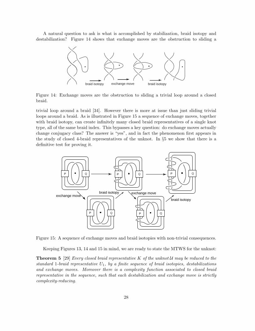
A natural question to ask is what is accomplished by stabilization, braid isotopy anddestabilization? Figure 14 shows that exchange moves are the obstruction to sliding a

braid isotopy braid isotopyexchange move

Figure 14: Exchange moves are the obstruction to sliding a trivial loop around a closedbraid.

trivial loop around a braid [34]. However there is more at issue than just sliding trivialloops around a braid. As is illustrated in Figure 15 a sequence of exchange moves, togetherwith braid isotopy, can create infinitely many closed braid representatives of a single knottype, all of the same braid index. This bypasses a key question: do exchange moves actuallychange conjugacy class? The answer is “yes”, and in fact the phenomenon first appears inthe study of closed 4-braid representatives of the unknot. In §5 we show that there is adefinitive test for proving it.

P P

exchange move

P

braid isotopy

P

P

exchange move

braid isotopy

Q Q

QQ Q

Figure 15: A sequence of exchange moves and braid isotopies with non-trivial consequences.

Keeping Figures 13, 14 and 15 in mind, we are ready to state the MTWS for the unknot:

Theorem 5 [29] Every closed braid representative K of the unknot U may be reduced to thestandard 1-braid representative U1, by a finite sequence of braid isotopies, destabilizationsand exchange moves. Moreover there is a complexity function associated to closed braidrepresentative in the sequence, such that each destabilization and exchange move is strictlycomplexity-reducing.

28

The first proof of Theorem 5 was the one in [29]. A somewhat different and slickerproof can be found in [21], but it requires more machinery than was necessary for presentpurposes. We follow the proof in [29]. However, parts of our presentation and most ofour figures were essentially lifted (with the permission of both authors) from [21], a reviewarticle on braid foliation techniques. Our initial goal is to set up the machinery needed forthe proof.

Recalling the definition of a closed braid from §2.1, we adopt some additional structureand say that K is in closed n-braid form if there is an unknot A in S3 \K, and a choice offibration H of the solid torus S3 \A by meridian disks, such that K intersects each fiber ofH transversely. Sometimes it is convenient to replace S3 by R3 and to think of the fibrationH as being by half-planes {Hθ; θ ∈ [0, 2π]} of constant polar angle θ through the z-axis.Note that K intersects each fiber Hθ in the same number of points, that number being theindex n of the closed braid K. We may always assume that K and A can be oriented sothat K travels around A in the positive direction, using the right hand rule. Now let K bea closed braid representative of the unknot, and let D denote a disk spanned by K, orientedso that the positive normal bundle to each component has the orientation induced by thaton K = ∂D. In this section we will describe a set of ideas which shows that there is avery simple method that changes the pair (K,D) to a planar circle that bounds a planardisc, via closed braids, moreover there is an associated complexity function that is strictlyreducing. The ideas that we describe come from [29], however our main reference will be tothe review article [21].

The braid axis A and the fibers of H will serve as a coordinate system in 3-space inwhich to study D. A singular foliation of D is induced by its intersection with fibers of H.A singular leaf in the foliation is one which contains a point of tangency with a fiber of H.All other leaves are non-singular.

It follows from standard general position arguments that the disk D can be chosen tobe ‘nice’ with respect to our fibration. More precisely, we can assume the following:

(i) The intersections of A and D are finite in number and transverse.

(ii) There is a neighborhood NA of A in R3 \K such that each component of D ∩NA isa disk, and each disk is radially foliated by its arcs of intersection with fibers of H.There is also a neighborhood NK of K in R3 such that NK ∩ D is foliated by arcs ofintersection with fibers of H which are transverse to K.

(iii) All but finitely many fibers Hθ of H meet D transversely, and those which do not(the singular fibers) are each tangent to D at exactly one point in the interior ofboth D and Hθ. Moreover, each point of tangency is a saddle point (with respect tothe parameter θ). Finally, each singular fiber contains exactly one singularity of thefoliation, each of which is a saddle point.

It can also be assumed (see [21] for details) that

(iv) Each non-singular leaf is either an a-arc, which has one endpoint on A and one onK = ∂D or a b-arc, which has both endpoints on A.

29

(vii) Each b-arc in a fiber Hθ separates that fiber into two components. Call the b-arcessential if each of these components is pierced at least once by K, and inessentialotherwise. Then we also have that all b-arcs in the foliation of D may be assumed tobe essential.

Note that D cannot be foliated entirely by b-arcs, since such a surface is necessarilya 2-sphere. Thus, if the foliation of D contains no singularities, D is foliated entirely bya-arcs. Otherwise, let U be the union of all the singular leaves in the foliation of D. Movingforward through the fibration, we see that any singular leaf in the foliation is formed bynon-singular leaves moving together to touch at a saddle singularity. The three types ofsingular leaves which can occur are labelled aa, ab or bb, corresponding to the non-singularleaves associated to them. Now each singular leaf λ in U has a foliated neighborhood Nλ

in D such that Nλ ∩ U = λ. According to whether λ has type aa, ab, or bb, Nλ is one ofthe foliated open 2-cells shown in Figure 16(i), with the arrows indicating the direction ofincreasing θ.

Type bb Type ab Type aa

s s1

2

3v

v

v

4v

1

2

3v 1v

v

v3

v

A

ss

A

s

A

v v

v

v

4 3

1

2

v

v

v

3

1

2

v

v

3

1

(i)

(ii)

s

Figure 16: (i) The three types of tiles in the decomposition of D; (ii)The canonical embed-ding of each type of tile.

The complement of U in D is a union B1∪B2∪ ...∪Bk, where each Bi is foliated entirelyby a-arcs or entirely by b-arcs. Choose one non-singular leaf in each Bi and declare it to bea boundary arc of type a or type b according to whether it is an a-arc or b-arc, respectively.Then the union of all boundary arcs determines a tiling of D, that is, a decomposition intoregions called tiles, each of which is a foliated neighborhood of one singular leaf. Each tilehas type aa, ab and bb, according to the type of its unique singularity. Note that a tilingof D is a foliated cell-decomposition. We further define the sign of a singular point s in thefoliation of D to be positive if the positive normal to D points in the direction of increasingθ in the fibration, negative otherwise. The sign of a tile is then defined to be the sign of its

30

singularity.The axis A intersects the surface in a finite number of points, called vertices of the tiles.

Each vertex v is an endpoint of finitely many boundary arcs in the surface decomposition.Let the type of v be the cyclic sequence (x1, ..., xr), where each xi is either a or b, and thesequence lists the types of boundary arcs meeting at v in the cyclic order in which theyoccur in the fibration. See Figure 17. The valence of a vertex v is the number of distinct

vv

w

type (a,b)type (a)

type (b,b)

q s+ -

α

α ’

α ’

a

w wv1 2

q

s

Figure 17: A vertex v of type (a), (ab) and (bb).

tiles intersecting at v. The sign of a vertex v is the cyclic array of signs of the tiles meetingat v. See Figure 17.

The parity of v is said to be positive (resp. negative) if the outward-drawn normal tothe surface has the same (resp. opposite) orientation as the braid axis at the vertex. Thuswhen we view the positive side of the surface, the sense of increasing θ around a vertexwill be counterclockwise (resp. clockwise) when the vertex is positive (resp. negative), asillustrated in Figure 16(i).

Finally, we note that (again, see [21] for a proof) that, up to a choice of their sign, tilesof type aa, ab, bb each have a canonical embedding in 3-space, which is determined up to anisotopy of 3-space which preserves the axis A and each fiber of H setwise. The canonicalembedding for each tile is shown in Figure 16(ii).

The decompositions of the disk D which we have just described are not unique. Weshall now describe three ways in which they can be changed. In each of the three cases thepossibility of making the change is indicated by examining the combinatorics of the tiling.The change is realized by an isotopy of the disk which is supported in a neighborhood Nof a specified small number of tiles of type aa, ab or bb, leaving the decomposition of Dunchanged outside N .

For a spanning disk D and a tiling T , we denote the complexity of the tiling by c(D,T ),where we define c(D,T ) = (n, S), where n is the braid index of the boundary and S is thenumber of singularities in the tiling. Setting V+ and V− equal to the number of positive andnegative vertices, one has n = V+ − V−, so n is also determined by the tiling. Tiled discs(D,T ) can then be ordered, using lexicographical ordering of the associated pair c(D,T ).Each of our three moves will replace the given disk and tiling D,T with some D′,T ′, withthe following effects on complexity:

• Change in foliation: (n′, S′) = (n, S).

31

• Destabilization: (n′, S′) = (n− 1, S − 1).

• Exchange moves (two types): (n′, S′) = (n, S − 2).

We focus here only on the combinatorics of tilings which admit one of the above moves,as well as the effect of each move on the embedding of D and the new tiling of D whichresults. For proof and further details, see [21].

•Changes in foliation. The choice of a foliation of D is not unique, and our first moveinvolves ways in which the surface decomposition can be changed by an isotopy of D or,equivalently, by an isotopy of the fibers of H keeping D fixed. This particular change wasintroduced in [28] for 2-spheres and was modified in [29] for certain spanning surfaces. Inwhat follows, we say that two tiles are adjacent if they have a common boundary arc in thegiven tiling.

1

1

2

2

1

2

6

3 5

4

SS

∆

µ

2 6 4

∆

µ

31 5

s ’

s ’’

’

θ θ

K

K

K

K

v v

w w

K

K

v

w

γ

ors’

s’

1

2 s’

s’

1

2

2s s1

(i)

(ii)

Figure 18: Sketch (i) shows an isotopy of D that induces a change in foliation. Sketch (ii)shows the effect of the change on two ab-tiles

A tiling admits a change in foliation whenever there are two tiles T1, T2 of the samesign adjacent at a b-arc. Roughly speaking, a change in foliation is a local isotopy of thesurface which pushes two saddle points past each other. Locally, the disk D is embedded asin the left sketch in Figure 18(i). A change in foliation is defined as the passage from theembedding left to the right embedding. Figure 18(ii) the effect of this move on the localfoliation, while Figure 18(iii) illustrates the effect of a change in foliation on the tiling, inthe case of two adjacent (ab)-tiles.

•Destabilization via a type (a) vertex. A vertex v of valence 1 in a tiling of D occurswhen two of the edges in a single tile T are identified in D. Such a vertex must have type(a), and therefore T is an aa-tile. See Figure 17. Since there is a canonical embedding foran aa-tile in 3-space (Figure 16), identifying two edges of an aa-tile with endpoints on acommon vertex yields the canonical embedding for T shown in Figure 19(i). Notice thatthere is a radially foliated disk D in T cut off from D by the arc of the singular leaf of T

32

with both endpoints on K. Hence there must be a trivial loop in the braid representationof K, and we can modify the braid and the disk D in the manner illustrated. We call thismodification destabilization via a type (a) vertex. The effect on the tiling of D is that theaa-tile T and its type (a) vertex v are deleted, while the tiling outside T is unaltered. Thebraid index is decreased by one. See the right sketch in Figure 19(i).

A A A

isotopyof K

v

K

D

(i) (ii)

v v

K

exchange

Figure 19: The effect of (i) a destabilization, and (ii) an exchange move of type (bb), onthe embedded (and foliated) foliated disc D and on the braid K that is its boundary.

•Exchange moves. The destabilization move that we just described can be accomplishedif a vertex of valence 1 exists in our tiling. Exchange moves are based upon the existenceof a vertex of valence 2. An example of the type of move we would like to achieve on thebraid itself was shown in sketch (ii) of Figure 19(ii), and also in in the second row from thetop in Figure 20. There are two different types of tiling patterns, and hence two differenttypes of local embeddings of D, which support exchange moves:

Exchange Move Type (bb): We now consider a vertex v with sign (±,∓) and type(b, b). In this situation, two bb-tiles are adjacent along consecutive b-arcs. The canonicalembeddings of the tiles in this case are shown in Figure 16, and the overall modifications toD are suggested by Figure 19(ii). The end result is a new surface D′ whose decompositionhas at least two fewer vertices (in particular, the vertex v is deleted) and at least two fewerregions than the decomposition of D. ‖

Exchange Move, Type (ab) An exchange move of type (ab) is possible whenever thetiling of D has a vertex v of valence 2, type (a,b), and sign (±,∓). Such a vertex occursonly when two ab-tiles are adjacent along corresponding a and b edges, as in Figure 17. Theisotopy of ∂D = K is achieved by pushing a subarc α of K across a disk which is containedin the union of two (ab) tiles T1, T2, to a new arc α′. The effect on the tiling is that theab-tiles T1 and T2 are deleted and any adjacent ab-tiles (resp. bb-tiles) become aa-tiles (resp.ab-tiles).

In order to prove the MTWS for the unknot, we must locate the places on the tilingof D where the three moves just described can be made. We begin with two lemmas. Thefirst of the two is implicit in [9], but we refer the reader to [21] for an explicit proof.

33

Lemma 3.1 [9] Let v be a vertex of type (b, b, . . . , b). Then the set of all singularities swhich lie on a singular leaf ending at v contains both positive and negative singular points.

Lemma 3.2 [29] Suppose that the disk D is nontrivially tiled and has no vertices of valence1. Then the tiling of D contains a vertex of type (ab), (bb), or (bbb).

Proof. The proof is essentially an Euler characteristic argument. A tiling T of the diskD corresponds to a cell decomposition of the 2-sphere in the following way. Let V be thenumber of vertices in T , let E be the number of boundary arcs in T , which we will thinkof as edges, and let F be the number of tiles in T . Now let Σ be the 2-sphere obtainedby collapsing ∂D = K to a point. This gives a cell decomposition of Σ with V + 1 0-cells(vertices), E 1-cells (edges), and F 2-cells (faces). We know that the Euler characteristicχ(Σ) = 2, and therefore we have that V − E + F = 1. We also know that every face inour cell decomposition of Σ has 4 edges, and that every edge has 2 adjacent faces, and soE = 2F . We therefore have the following equation.

2V − E = 2. (10)

Now let V (α, β) denote the number of vertices in T with α adjacent a-arcs and β adjacentb-arcs. If v is the valence of such a vertex, then v = α+ β, and so V (α, v − α) denotes thenumber of vertices in T with valence v and α adjacent a-arcs. Since by hypothesis v 6= 1,we can now count the number of vertices in T using the following summation:

V =

∞∑

v=2

v∑

α=0

V (α, v − α)

Now write E = Ea+Eb, where Ea denotes the number of edges in T of type a, and similarlyfor Eb. Since an a-edge is incident at one vertex in T , and a b-edge is incident at two verticesin T , we can write:

Ea =

∞∑

v=2

v∑

α=0

αV (α, v − α) (11)

Eb =1

2

∞∑

v=2

v∑

α=0

(v − α)V (α, v − α) (12)

Substituting into Equation 10, we now have

∞∑

v=2

v∑

α=0

(4 − v − α)V (α, v − α) = 4.

Observe now that if v ≥ 4, the coefficient (4 − v − α) ≤ 0. Writing out the termscorresponding to v = 2 and v = 3 gives, respectively, 2V (0, 2) + V (1, 1) and V (0, 3) −V (2, 1) − 2V (3, 0). Each V (α, β) ≥ 0 by definition. Hence we can move terms around inthe above equation so that each term is nonnegative, as follows:

2V (0, 2) + V (1, 1) + V (0, 3) = 4 + V (2, 1) + 2V (3, 0) +

∞∑

v=4

v∑

α=0

(4 − v − α)V (α, v − α).

34

The right-hand side of the equation is clearly ≥ 4, and therefore at least one term on theleft-hand side is nonzero. Since V (0, 2), V (1, 1), and V (0, 3) record the number of type (bb),type (ab), and type (bbb) vertices, respectively, the lemma is proved. ‖

We are now ready to prove Theorem 5, the MTWS in the case of the unknot.

Proof of Theorem 4. We start with an arbitrary closed braid representative K of theunknot. Our closed braid K is the boundary of a disk D which admits a tiling T . Note thatif the complexity of the tiling c(D,T ) is equal to (1, 0), then our disk is radially foliated by a-arcs and K is the standard embedding of the unknot. Therefore we assume c(D,T ) > (1, 0).We will use induction on c(D,T ) to show that after a finite sequence of our three moves, Dis radially foliated by a-arcs.

We first observe that if there exists a vertex of type (a) in T , then we can destabilizealong this vertex, thereby reducing c(D,T ). Hence we can asume that all vertices in Thave valence at least 2. By Lemma 3.2, D must have a vertex of type (ab), (bb), or (bbb). Ifthere is a type (bbb) vertex, then at least two of the adjacent tiles must have the same sign.In this case we can do a change in foliation, replacing our (bbb) vertex with a (bb) vertex.Therefore we may assume that D contains a vertex of type (ab) or type (bb).

If D has a type (ab) vertex with sign (+,+) or (-,-), then we can apply a change infoliation which replaces this vertex with a type (a) vertex. We now destabilize along thistype (a) vertex in order to reduce the complexity. If D has a type (ab) vertex with sign (+,-), then we can do an exchange move of type (ab), thereby reducing complexity. If D has atype (bb) vertex, then it is an interior vertex, and by Lemma 3.1, it has sign (+,-). Thenwe can do an exchange move of type (bb), which reduces complexity.

Thus if c(D,T ) > (1, 0), we can always reduce until c(D,T ) = (1, 0), and the theoremis proved. ‖

Example 3.1 [Morton’s irreducible 4-braid] We now give an example illustrating thenecessity of exchange moves. In [109], Morton gave the following example of an irreduciblebraid:

X = σ−23 σ2σ

−13 σ2σ

31σ

−12 σ1σ

−12 ,

i.e., a braid whose closure represents the unknot but cannot be isotoped to the unknot in thecomplement of the braid axis. Now, it is clear that if a braid in Bn admits a factorizationof the form w1σn−1w2σ

−1n−1, where w1 and w2 are words in σ1, . . . , σn−2, then its closure

admits an exchange move. As observed in [29], the conjugate braid (σ3σ2σ1)X(σ−11 σ−1

2 σ−13 )

is isotopic to the braidX ′ = (σ−2

2 σ1σ−12 )σ3(σ

32σ

−11 σ2)σ

−13 .

ThusX ′ admits an exchange move to obtain the new braid word (σ−22 σ1σ

−12 )σ−1

3 (σ32σ

−11 σ2)σ3,

which can be cyclically rewritten as

X ′′ = (σ2σ3σ−22 )σ1(σ

−12 σ−1

3 σ32)σ

−11 .

If we now interchange the axis of our braid with the point at infinity, we can perform anotherexchange move to obtain

X ′′′ = (σ2σ3σ−22 )σ−1

1 (σ−12 σ−1

3 σ32)σ1

35

which can in fact be isotoped to the unknot in the complement of its braid axis [29].Wright has given a foliated disk corresponding to this braid in [133]. The reader is

cautioned that Wright uses a different notation convention for braid words than that usedin this paper (see p. 98 of [133]). We also refer the reader to [32] for further examples. ♠

We note that Theorem 5 has been used as the basis for an algorithm for recognizing theunknot. See [22]. This algorithm has been put on a computer [32], however it needs morework before it can become a practical tool for recognizing the unknot.

Open Problem 2 At this writing the development of a sound and practical algorithm forunknot recognition remains one of the major open problems in low dimensional topology. ♣

With regard to Problem 2, we note that Theorem 5 proves the existence of a monotonicsimplification process which begins with an arbitrary closed n-braid representative of theunknot and ends with a 1-braid representative, but the complexity function c(D,T ) whichgives instructions for the process is ‘hidden’ in the tiling of the surface D. We need it inorder to know when complexity-reducing destabilizations and exchange moves are possible.The reader who is interested in this problem might wish to consult [22], where a somewhatdifferent approach suggests itself. Instead of working with the tiled surface, one may workwith the ‘extended boundary word’ of [22]. The latter is a closed braid which is obtainedfrom an arbitrary closed braid representative of the given knot by threading in additional1-braids, and it seems likely that it will give an alternative monotonic reduction process.Thus we suggest:

Open Problem 3 Investigate the monotonic reduction process of Theorem 5 from the pointof view of the extended boundary word of [22]. ♣

3.2 The Markov Theorem Without Stabilization, general case

In this section we state the generalized version of Theorem 5 which was established in [30]for arbitrary closed braid representatives of arbitrary knots and links. The moves whichare needed are of course much more complicated than in the case of the unknot. They aredescribed in terms of ‘block strand diagrams’ and ‘templates’. The concept of a block-stranddiagram is fairly easy to understand from the 8 examples in Figure 20. The first importantfeature of a block-strand diagram is that after an assignment of a braided tangle to eachblock, it becomes a closed braid that represents a specific knot or link. Thus each blockstrand diagram determines infinitely many closed braid representatives of (presumably)infinitely many knots and links. A template is a pair of block-strand diagrams, both ofwhich represent the same knot or link, when we make the same braiding assignments tocorresponding blocks. Note that there are two destabilization templates (they differ in thesign of the ‘trivial loop’ that is removed). There are also two flype templates, which differin the sign of the single crossing which is outside all the braid boxes. Templates alwayshave an associated braid index, namely the braid index of any knot or link of minimumbraid index that they carry. Destabilization templates occur for every braid index ≥ 2.Since the exchange move can be realized by braid isotopy when the braid index is ≤ 3, itdoes not play a role until braid index ≥ 4. The flype templates occur for braid index ≥ 3.

36

A A

PP

1 1

w wA A

PP

1 1

w w+ -

w w

P PQ Q

The exchange move template

A A

P

Q

R

P

Q

R + +A A

P

Q

R

P

Q

R --A A

w w’

k

k’

w’k

k’w

w’

k

k’ w’

kk’

ww

The two destabilization templates

The two flype templates

W

Y

X

Z

W

Y

Z

X

A 6-braid template

Figure 20: Examples of templates

37

The method by which the 6-braid template in Figure 20 was constructed is described in themanuscript [30].

The two block strand diagrams in a template are always related by a sequence of Markovmoves, however the sequence may be quite complicated, and so the isotopy that takes theleft diagram to the right diagram is in general not obvious. This fact is illustrated by the6-braid template of Figure 20. (See [30] for the isotopy, as an explicit sequence of Markovmoves.)

With this brief introduction, we are able to state the Markov Theorem Without Stabi-lization in the general case:

Theorem 6 [30] Let B be the collection of all braid isotopy classes of closed braid repre-sentatives of oriented knot and link types in oriented 3-space. Among these, consider thesubcollection B(K) of representatives of a fixed link type K. Among these, let Bmin(K)be the subcollection of representatives whose braid index is equal to the braid index of K.Choose any X+ ∈ B(K) and any X− ∈ Bmin(K). Then there is a complexity functionwhich is associated to X+,X−, and for each braid index m a finite set T (m) of templates isintroduced, each template determining a move which is non-increasing on braid index, suchthat the following hold: First, there is are initial sequences which modify X− → X ′

− andX+ → X ′

+:

X− = X1− → · · · → Xp

− = X ′−, X+ = X1

+ → . . .→ Xq+ = X ′

+

Each passage Xj− → Xj+1

− is strictly complexity reducing and is realized by an exchange

move, so that b(Xj+1− ) = b(Xj

−). These moves ‘unwind’ X−, if it is wound up as in the

top right sketch in Figure 15. Each passage Xj+ → Xj+1

+ is strictly complexity-reducing

and is realized by either an exchange move or a destabilization, so that b(Xj+1+ ) ≤ b(Xj

+).Replacing X+ with X ′

+ and X− with X ′−, there is an additional sequence which modifies

X ′+, keeping X ′

− fixed:X ′

+ = Xq → · · · → Xr = X ′−

Each passage Xj → Xj+1 in this sequence is also strictly complexity-reducing. It is realizedby one of the moves defined by a template T in the finite set T (m), where m = b(X+).The inequality b(Xj+1) ≤ b(Xj) holds for each j = q, . . . , r − 1 and so also for each j =1, . . . , r − 1.

The proof of Theorem 6 uses the braid foliation techniques that were used in the proofof Theorem 5, but in a more complicated setting. Instead of looking at a foliated embeddeddisc which is bounded by a given unknotted closed braid, we are given two closed braids,X+ and X−, and an isotopy that takes X+ to X−. The trace of the isotopy sweeps out anannulus, but in general it is not embedded. The proof begins by showing that the givenisotopy can be split into two parts, over which we have some control. An intermediate linkX0 which represents the same link type K as X+ and X− is constructed, such that the traceof the isotopy from X+ to X0 is an embedded annulus A+. Also the trace of the isotopyfrom X0 to X− is a second embedded annulus A−. The union of these two embedded annuliT A = A+ ∪ A− is an immersed annulus, but its self-intersection set is controlled, and is afinite number of clasp arcs. The main tool in the proof of Theorem 6 is the study of the

38

braid foliation of the immersed annulus T A. In the next section, i.e. §3.3, we will see howTheorem 6 was used to settle a long-standing problem about contact structures.

3.3 Braids and contact structures

In this section we describe how Theorem 6 was used in [31] to settle a problem about contactstructures on R

3 and S3.Let A be the z-axis in R

3, with standard cylindrical coordinates (ρ, θ, z) and let H bethe collection of all half-planes Hθ through A. The pair (A,H) defines the standard braidstructure on R

3. Using the same cylindrical coordinates, let α be the 1-form α = ρ2dθ+dz.The kernel ξ of the 1-form α defines a contact structure on R

3. We can visualize ξ byimagining that there is a 2-plane (spanned by ∂/∂x and ∂/∂ρ) attached to every pointin R

3. Figure 21 shows both the braid structure and the polar contact structure, forcomparison. The family of 2-planes that define ξ twist (to the left) as one moves along thex-axis from 0 to ∞. The family is invariant under rotation of 3-space about the z-axis andunder translation of 3-space along rays parallel to the z-axis. Its salient feature is that it istotally non-integrable, that is there is no surface in R

3 which is everywhere tangent to the2-planes of (ξ) in any neighborhood of any point in R

3. (Of course this makes it hard tovisualize). The twisting is generic in the sense that, if p is a point in a contact 3-manifoldM3, then in every neighborhood of p in M3 the contact structure is locally like the one wedepicted in Figure 21.

zz z

θH

θ

θ

H

H1

2

K

K

standard tight polar contact structurestandard braid structure

Figure 21: The standard braid structure and tight contact structure on R3

Let K be a knot (for simplicity we restrict to knots here, but everything works equallywell for links) which is parametrized by cylindrical coordinates (ρ(t), θ(t), z(t)), where t ∈[0, 2π]. Then, as defined in §2.1, K is a closed braid if ρ(t) > 0 and dθ/dt > 0 for all t.On the other hand, K is a Legendrian (resp. transversal) knot if it is everywhere (resp.nowhere) tangent to the 2-planes of ξ. In the Legendrian case this means that on K we havedθ/dt = (−1/ρ2)(dz/dt). In the transversal case we require that dθ/dt > (−1/ρ2)(dz/dt)at every point of K(t). We are interested here primarily in the transversal case.

The total twist of the contact structure is the number of multiples of π/2 as one traversesthe positive real axis from the origin to ∞. The case when the total twist angle is π is knownas the standard (polar) contact structure. We call it ξπ. While the braid structure is very

39

different from the standard polar contact structure near A, for large values of ρ the 2-planes in ξπ are very close to the half-planes Hθ of the braid structure. In fact, assumethat X is a closed braid which represents a knot K, and that X bounds a Seifert surface ofminimum genus which supports a foliation as in §3.1. Assume further that the closed braidX intersects every 2-plane in the contact structure transversally. Then, in the complementof a tubular neighborhood of the braid axis, from the point of view of a topologist, the braidfoliation and the foliation induced by the contact structure will be ‘the same’.

Recall that Theorem 2 (Alexander’s Theorem) was first proved in 1925. Sixty years later,Bennequin adapted Alexander’s original proof (which is different from the proof given in thisarticle) to the setting of transversal knots in [9], where he showed that every transversal knotis isotopic, through transversal knots, to a closed braid. In 2002 Orevkov and Shevchishinextended Bennequin’s ideas and proved a version of Theorem 4 (Markov’s Theorem) whichholds in the transversal setting:

Theorem 7 [116]: Let TX+, TX− be closed braid representatives of the same oriented linktype K in oriented 3-space. Then there exists a sequence of closed braid representatives ofT K:

TX+ = TX1 → TX2 → · · · → TXr = TX1

such that, up to braid isotopy, each TXi+1 is obtained from TXi by a single positive stabi-lization or destabilization.

Is the Transverse Markov Theorem really different from the Markov Theorem? Are theretransversal knots which are isotopic as topological knots but are not transversally isotopic?To answer this question we take a small detour and review the contributions of Bennequinin [9].

Why did topologists begin to think about contact structures, and analysts begin to thinkabout knots? While we might wish that analysts suddenly became overwhelmed with thebeauty of knots, there was a more specific and focused reason. At the time that Bennequindid his foundational work in [9] it was not known whether a 3-manifold could supportmore than one isotopy class of contact structures. Bennequin answered this question in theaffirmative, in the case of contact structures on R

3 or S3 which were known to be homotopicto the standard one. His tool for answering it was highly original, and it had to do withbraids and knots.

Let TK be a transversal knot. By the above, we can assume without loss of generalitythat it is a closed braid. Let T K be its transversal knot type, i.e., its knot type undertransversal isotopies, and let [T K]top be its topological knot type. Choose a representativeTX of T K, which (by Bennequin’s transversal version of Alexander’s theorem) is alwayspossible. Choose a Seifert surface F of minimal genus, with TX = ∂F . Bennequin studiedthe foliation of F which is induced by the intersections of F with the plane field determinedby ξπ. Let n(TX) be the braid index and let e(TX) be the algebraic crossing numberof a projection of TX onto the plane z = 0. Both can be determined from the foliation.Bennequin found an invariant of T K, given by the formula β(T K) = e(TX) − n(TX). Ofcourse if he had known Theorem 7 the proof that β(T K) is an invariant of T K would havebeen trivial, but he did not have that tool. He then showed a little bit more: he showed thatβ(T K) is bounded above by the negative of the Euler characteristic of F in ξπ. He then

40

showed that this bound fails in one of the contact structures ξ>π. In this way he provedthat the contact structures ξ>π cannot be isotopic to ξπ.

To knot theorists, Bennequin’s proof should seem intuitively natural, because the in-variant β(T K) is a self-linking number of a representative TX ∈ T K (the sense of push-offbeing determined by ξ), and the more twisting there is the higher this number can be. Foran explanation of the self-linking, and lots more about Legendrian and transversal knots werefer the reader to John Etnyre’s excellent review article [63]. The basic idea is that TXbounds a Seifert surface, and this Seifert surface is foliated by the plane field associatedto ξ. Call this foliation the characteristic foliation. Near the boundary, the characteristicfoliation is transverse to the boundary. The Bennequin invariant is the linking number ofTX, TX ′, where TX ′ is is a copy of TX, obtained by pushing TX off itself onto F , usingthe direction determined by the characteristic foliation of F .

Bennequin’s paper was truly important. Shortly after it was written Eliashberg showedin [59] that the phenomenon of an infinite sequence of contact structures related to a singleone of minimal twist angle occured generically in every 3-manifold, and introduced the term‘tight’ and ‘overtwisted’ to distinguish the two cases. Here too, there is a reason that willseem natural to topologists. In 2003 Giroux proved [79] that every contact structure onevery closed, orientable 3-manifold M3 can be obtained in the following way: represent M3

as a branched covering space of S3, branched over a knot or link, and lift the standard andovertwisted contact structures on S3 to M3.

Returning to knot theory, the invariant β(T K) allows us to answer a fundamental ques-tion: is the equivalence relation on knots that is defined by transversal isotopy really differ-ent from the equivalence relation defined by topological isotopy? The Bennequin invariantwill be used to answer this question in the affirmative:

Theorem 8 [9] There are infinitely many distinct transversal knot types associated to eachtopological knot type.

Proof: Choose a transversal knot type T K and a closed braid representative TX0. Sta-bilizing the closed braid TX0 once negatively (recall the definition of positive/negativestabilizations given in §2.3, Figure 7), we obtain the transverse closed braid TX1, withe(TX1) = e(TX0) − 1 and n(TX1) = n(TX0) + 1, so that β(TX1) = β(TX0) − 2. It-erating, we obtain transverse closed braids TX2, TX3, . . ., defining transverse knot typesT K1,T K2,T K3, · · ·, and no two have the same Bennequin invariant. Since stabilizationdoes not change the topological knot type, the assertion follows. ‖

At this writing, it is an open problem to find computable invariants of T K which arenot determined by [T K]top and β(T K). A hint that the problem might turn out to be quitesubtle was in the paper [72] by Fuchs and Tabachnikov, who proved that while ragbagsfilled with polynomial and finite type invariants of transversal knot types T K exist, basedupon the work of Arnold in [5], they are all determined by [T K]top and β(T K). Thus, theseemingly new invariants that many people had discovered by using Arnold’s ideas werejust a fancy way of encoding [T K]top and β(T K).

This leads naturally to a question: Are there computable invariants of transversal knotswhich are not determined by [T K]top and β(T K)? A similar question arises in the settingof Legendrian knots. Each Legendrian knot LK determines a topological knot type [LK]top,

41

and just as in the transverse case it is an invariant of the Legendrian knot type. Thereare also two numerical invariants of LK: the Thurston-Bennequin invariant tb(LK) (a self-linking number) and the Maslov index M(LK) (a rotation number). So until a few years agothe same question existed in the Legendrian setting, but the Legendrian case has recentlybeen settled by Yuri Chekanov:

Theorem 9 [45] There exist distinct Legendian knot types which have the same topologicalknot type[LK]top, and also the same Thurston-Bennequin invariant tb(LK) and Maslov indexM(LK).

The analogous result for transversal knots proved to be quite difficult, so to begin tounderstand whether something could be done via braid theory, the first author and NancyWrinkle asked an easier question, which they answered in part in [34]: are there transversalknot types which are determined by their topological knot type and Bennequin number?This question lead to a definition: a transversal knot type T K is transversally simple if itis determined by [T K]top and β(T K). So the question is: are there transversally simpleknots? The manuscript [34] gives a purely topological (in fact braid-theoretic) criterionwhich enables one to answer the question affirmatively, adding one more piece of evidencethat topology and analysis walk hand in hand. To explain it, recall the destabilization andexchange moves, and the two flypes, depicted in Figure 20. A topological knot or link typeK is said to be exchange reducible if an arbitrary closed braid representative X of K can bechanged to an arbitrary representative of minimum braid index by braid isotopy, positiveand negative destabilizations and exchange moves. We have:

Theorem 10 [34] If a knot type K is exchange-reducible, then any transversal knot typeT K which has [T K]top = K is transversally simple.

This theorem was used to give a new proof of a theorem of Eliashberg [60], which asserts thatthe unlink is transversally simple, and also (with the help of [105]) to prove the then-newresult that most iterated torus knots are transversally simple.

The rest of this section will be directed at explaining the main result of [31]:

Theorem 11 [31] There exist transversal knot types which are not transversally simple.Explicitly, the transverse closed 3-braids TX+ = σ5

1σ42σ

61σ

−12 and TX− = σ5

1σ−12 σ6

1σ42 deter-

mine transverse knot types T K+,T K− with (T K+)top = (T K−)top and β(T K+) = β(T K−),but T K+ 6= T K−.

Sketch of the proof of Theorem 11. See [31] for all details. The examples in Theorem11 were obtained by choosing all the weights in the negative flype template to be 1, andassigning explicit 2-braids to the blocks P,Q,R of the negative flype template of Figure20. If the weights are all chosen to be 1, the blocks P,Q,R are 2-braids and (except invery special cases) the flype templates have braid index 3. First one must show that theexamples satisfy the conditions of the theorem. The topological knot types defined by theclosed 3-braids σ5

1σ42σ

61σ

−12 and σ5

1σ−12 σ6

1σ42 coincide because they are carried by the block

strand diagrams for the negative flype template of Figure 20. The Bennequin invariant canbe computed as the exponent sum of the braid word (14 in both cases) minus the braidindex (3 in both cases). So the examples have the required properties.

42

The hard part is the establishment of a special version of Theorem 6 which is applicableto the situation. Its special features are as follows:

1. Both X+ and X− have braid index 3.

2. Since it is well known that exchange moves can be replaced by braid isotopy for3-braids, the first two sequences in Theorem 6 are vacuous, i.e. X± = X ′

±.

3. Because of the special assumption just noted, the templates that are needed, in thetopological setting, can be enumerated explicitly: they are the positive and negativedestabilization and the positive and negative flype templates. No others are needed.

It is proved in [31] that if X− and X+ are transversal closed braids TX+ and TX−,then the isotopy that takes TX+ to TX− may be assumed to be transversal. So, supposethat a transversal isotopy exists from the transverse closed braid TX+ to the transverseclosed braid TX−. Then there is a 3-braid template that carries the braids σ5

1σ42σ

61σ

−12 and

σ51σ

−12 σ6

1σ42. This is the first key fact that we use from Theorem 6. Instead of having to

consider all possible transversal isotopies from TX+ to TX−, we only need to consider thosethat relate the left and right block-strand diagrams in one of the four 3-braid templates. Sothe braids in question are carried either by one of the two destabilization templates or byone of the two flype templates. If it was one of the destabilization templates, then the knotsin question could be represented by 2 or 1-braids, i.e. they would be type (2, n) torus knotsor the unknot, however an easy argument shows that the knots in Theorem 11 are neithertype (2, n) torus knots or the unknot. The positive flype templates are ruled out in differentway: topologically, our closed braids admit a negative flype, so if they are also carried bythe positive flype template they admit flypes of both signs. However, the manuscript [93]gives conditions under which a closed 3-braid admits flypes of both signs, and the exampleswere chosen explicitly to rule out that possibility.

We are reduced to isotopies that are supported by the negative flype template. It isstraightforward to show that the obvious isotopy is not transversal, but maybe there issome other isotopy which is transversal. Here a key fact about the definition of a templateis used (and this is a second very strong aspect of the MTWS). If such a transversal isotopyexists, then it exists for every knot or link defined by a fixed choice of braiding assignmentsto the blocks. Choose the braiding assignments σ3

1, σ42 , σ

−51 to the blocks P,R,Q. This

braiding assignment gives a 2-component link L1⊔L2 which has two distinct isotopy classesof closed 3-braid representatives. If L1 is the component associated to the left strandentering the block P , then β(L1) = −1 and β(L2) = −3 before the flype, but after theflype the representative will be σ3

1σ−12 σ−5

1 σ42 , with β(L1) = −3 and β(L2) = −1. However,

by Eliashberg’s isotopy extension theorem (Proposition 2.1.2 of [60]) a transversal isotopyof a knot/link extends to an ambient transversal isotopy of the 3-sphere. Any transversalisotopy of L1 ⊔ L2 must preserve the β-invariants of the components. It follows that nosuch transversal isotopy exists, a contradiction of our assumption that TX+ and TX− aretransversally isotopic. ‖

Other examples of a similar nature were discovered by Etnyre and Honda [64] afterthe proof of Theorem 11 was posted on the arXiv. Their methods are very different from

43

the proof that we just described (being based on contact theory techniques rather thantopological techniques), but are equally indirect. They do not produce explicit examples,rather they present a bag of pairs of transverse knots and prove that at least one pair in thebag exists with the properties given by Theorem 11. Therefore we pose, as an importantopen problem:

Open Problem 4 Find new computable invariants of transversal knot types. Here ‘new’means an invariant which is not determined by the topological knot type T X and and theBennequin invariant β(T X ). ‘Computable’ means that it should be computable from eithera closed braid diagram or some other representation of the transversal knot. Braid groupsseem to be a natural setting for investigating this problem. ♣

Remark 3.1 The connections between closed braids and contact structures does not endwith transversal knots. There are fundamental relationships between open book structureson 3-manifolds and contact structures on those manifolds, both untwisted and twisted.See [79] for an introduction to this interesting new area, and see [63] for a review of themathematics and a discussion of many open problems waiting to be investigated.

44

4 Representations of the braid groups

Before the discovery of Hecke algbra representations of the braid group (discussed in thissection) very little was known about finite dimensional but infinite representations of Bn,except for the ubiquitous Burau representation. That matter changed dramatically in 1987with the publication of [89]. Suddenly, we had more knot invariants and with them morebraid group representations than anyone could deal with, and the issue became one oforganizing them. However, we shall not attempt to give a comprehensive overview of therich theory of representations of braid groups in this section. Instead, we focus here onthe representations of Bn which have played the greatest roles in the development of thattheory: the Burau representation, the Hecke algebra representations, and, more recently,the Lawrence-Krammer representation.

4.1 A brief look at representations of Σn

The fact that the representation theory of Bn is rooted in the representation theory of thesymmetric group Σn is a consequence of the surjection Bn → Σn, given by mapping theelementary braid σi to the transposition si = (i, i+ 1). While the kernel of this homomor-phism is very big (it’s the entire pure braid group Pn), it nevertheless turns out that a greatdeal can be learned about representations of Bn by studying the collection of irreduciblerepresentations of Σn, and attempting to lift them to reprentations of Bn by ‘deforming’them, and hoping that you get something new. For the record, we now note that the groupalgebra CΣn has generators 1, s1, . . . , sn−1 and defining relations:

sisk = sksi if |i− k| ≥ 2, sisi+1si = si+1sisi+1, s2i = 1, (13)

where 1 ≤ i 6= k ≤ n − 1. As a vector space, CΣn is spanned by n! reduced words [35] inthe transpositions si:

{(si1si1−1 . . . si1−k1)(si2si2−1 . . . si2−k2

) · · · (sirxir−1 . . . sir−kr)} (14)

where 1 ≤ i1 < i2 < · · · < ir ≤ n− 1 and ij − kj ≥ 1.Irreducible representations of Σn are parametrized by Young diagrams, which in turn

are parametrized by partitions of n. (See [73] for one of the many good discussions ofthis subject in the literature.) A Young diagram consists of stacked rows of boxes, alignedon the left, with the number of boxes in each row strictly nonincreasing as you go fromtop to bottom. The number of boxes in a row corresponds to a term in a given partitionof n. For example, the Young diagram shown in Figure 22 corresponds to the partition8 = 4 + 2 + 1 + 1.

Figure 22: The Young diagram corresponding to the partition 4 + 2 + 1 + 1.

45

As it turns out, the irreducible representations of the symmetric group are in 1-1 cor-respondence with Young diagrams, or equivalently with partitions of n. There is a row-column symmetry, and we adopt the convention that the Young diagram which has onerow of n boxes, which comes from the partition n = n, corresponds to the trivial repre-sentation. Then the Young diagram which has n rows consisting of 1 box per row, whichcomes from the partition n = 1 + 1 + · · · + 1, corresponds to the parity representation,mapping each element of Σn to its sign. The first interesting representation of a braidgroup occurs when n = 3, corresponding to the partition 3 = 2 + 1. More generally, weconsider the partition n = (n − 1) + 1, or the Young diagram with two rows, the top rowhaving (n− 1) boxes and the bottom having a single box. This Young diagram correspondsto the standard representation Σn → GLn(C), given by the usual action of Σn on C

n bypermuting basis vectors. Thus if si denotes the transposition (i i+ 1) ∈ Σn, the standardrepresentation sends si to the following:

Ii−1 ⊕(

0 11 0

)

⊕ In−i−1

where Ik denotes the k × k identity matrix.The standard representation is reducible; it is easy to see that it fixes a 1-dimensional

subspace, namely, the span of the sum of the basis vectors. The complementary (n − 1)-dimensional subspace is the set of all points (z1, . . . , zn) ∈ C

n such that z1 + . . . + zn = 0.This subspace corresponds to the irreducible representation given by the Young diagram inquestion. One can use the hook length formula to calculate directly that the dimension ofthe representation corresponding to this Young diagram is indeed n−1 (we refer the readeragain to [73] for an explanation of this formula).

4.2 The Burau representation and polynomial invariants of knots.

Burau first introduced his representation of the braid group in 1936 [42]. Much later, itwas realized that it could be thought of as a deformation of the standard representationof Σn corresponding to the partition n = (n − 1) + 1. For many years it was the focus ofthe representation theory of braid groups. We define the Burau representation ρ : Bn →GLn(Z[t, t−1]) as follows:

σi 7→ Ii−1 ⊕(

1 − t t1 0

)

⊕ In−i−1

Note that substituting t = 1 gives back the representation (of Bn factoring through Σn), andthis is why we say that it is a deformation of the standard representation of Σn. Like the rep-resentation of Σn, the Burau representation splits into a 1-dimensional representation and an(n − 1)-dimensional irreducible representation known as the reduced Burau representationwhich we denote by ρ : Bn → GLn(Z[t, t−1]) as follows:

σi 7→ Ii−2 ⊕

1 −t 00 −t 00 −1 1

⊕ In−i−2

where the −t in the middle of the 3 × 3 matrix is always in the (i, i)th spot.

46

It has been known for a long time that the Burau representation is faithful for n ≤ 3(see [18], for example), and for many years the representation was held to be a reasonablecandidate for a faithful linear representation of Bn for all n. However, in 1991, Moodyshowed that for n ≥ 9, the Burau representation is not faithful [107]. Long and Paton laterimproved Moody’s result to n ≥ 6 [103]. Bigelow further improved this to n ≥ 5 [13]. Atthe time of this writing, the case n = 4 remains open.

Despite such results, the Burau representation continues to play an important role inthe study of representations of Bn. It was known classically that the Alexander polynomial∆K(t) of a knot or link K can be calculated directly from the image under the reducedBurau representation of a braid X such that b(X) represents K, as follows (see [18], e.g.,for a proof based upon Theorem 4, the Markov Theorem):

∆b(X)(t) =det(ρ(X) − In−1)

1 + t+ · · · + tn−1. (15)

Thus the Alexander polynomial of the closed braid associated to the open braid X, i.e.∆b(X)(t), is a rescaling of the characteristic polynomial of the the image of X in the reducedrepresentation. In what follows, we shall see how a property of the Burau representationmotivated the definition of a variant on the two-variable HOMFLY polynomial [75], a knotinvariant of which both the Alexander polynomial and the Jones polynomial are specializa-tions. Further, in §4.4 we shall give a topological interpretation of the Burau representationwhich naturally leads to the definition of a faithful linear representation of Bn known asthe Lawrence-Krammer representation, which will be our focus in §4.5.

4.3 Hecke algebras representations of braid groups and polynomial in-variants of knots

A simple calculation, together with the Cayley-Hamilton theorem, shows that the imageof each of our braid group generators under the Burau representation, ρ(σi), satisfies thecharacteristic equation x2 = (1 − t)x + t and thus has two distinct eigenvalues. Thisprompted Jones to study all representations ρ : Bn → GLn(C) which have at most twodistinct eigenvalues [89]. Let xi = ρ(σi). Then for all i, xi must satisfy a quadratic equationof the form x2

i + axi + b = 0. By rescaling, we may assume that one of the eigenvaluesis 1 and eliminate one of the variables, e.g., a = −(1 + b). Note that by rewriting ourquadratic equation and making the substitution b = −t we regain the characteristic equationfrom the Burau representation. However, the convention in the literature seems to be torescale our representation by (−1) so that the equation takes the form x2

i = (t − 1)xi + t.With this motivation, we define the Hecke algebra Hn(t) to be the algebra with generators1, x1, . . . , xn−1 and defining relations as follows:

xixk = xkxi if |i− k| ≥ 2, xixi+1xi = xi+1xixi+1, x2i = (t− 1)xi + t, (16)

where 1 ≤ i 6= k ≤ n−1. Comparing the relations in (13) and (16), we see thatHn(1) ∼= CΣn,the group algebra of the symmetric group. Hence we can think of Hn(t) as a ‘deformation’of CΣn.

The connection between Hn(t) and CΣn is made even more transparent by noting that asa vector space, Hn(t) is spanned by n! lifts of a system of reduced words in the transpositions

47

si ∈ Σn. For example, we can take as a spanning set

{(xi1xi1−1 . . . xi1−k1)(xi2xi2−1 . . . xi2−k2

) · · · (xirxir−1 . . . xir−kr)} (17)

where 1 ≤ i1 < i2 < · · · < ir ≤ n− 1 and ij − kj ≥ 1 [35], [89].

Remark 4.1 In §1.4.2 we defined an algebra Jn(t) with generators 1, g1, . . . , gn−1 and defin-ing relations (7), the Jones algebra. As it turns out, its irreducible summands are in 1-1 cor-respondence with the irreducible representations of the Hecke algebra that are parametrizedby Young diagrams with exactly 2 rows. The Hecke algebra, as defined above, has gener-ators maps 1, x1, . . . , xn−1 with defining relations (16), so that the map ξ : Hn(t) → Jn(t)that is defined by ξ(xi) = gi is a homorphism of algebras.

Our main purpose in this section is to outline Jones’ development in [89] of a two-variablepolynomial knot invariant arising from representations of the Hecke algebras Hn(t). Thispolynomial is essentially the well-known HOMFLY polynomial, and includes the Jonespolynomial as a specialization. We have just seen that the Jones algebra is the quotient ofthe Hecke algebra Hn(t) by one extra relation (as an aside, we note that this extra relationis satisfied by the image of the transpositions generators si = (i, i + 1) in Σn under allrepresentations arising from Young diagrams with at most two rows.) To pick up a secondvariable, we introduce an additional parameter by allowing a 1-parameter family of traceson Hecke algebras. We now pursue this point of view, and we also refer the reader to [85]for another exposition which follows the same point of view.

We begin by defining a function f : Bn → Hn(t) by f(σi) = xi. The function f is well-defined on reduced words in the generators σi and commutes with the natural inclusionsBn−1 ⊂ Bn and Hn−1(t) ⊂ Hn(t), although in general f fails to be a homomorphism. Wecan then apply the following result due to Adrian Ocneanu which appeared in [75] and wasproved inductively in [89] using the n!-element basis given above.

Theorem 12 [75], [89] For each z ∈ C∗ (and each t ∈ C

∗), there exists a unique tracefunction tr : ∪∞

n=1Hn(t) → C such that

1. tr(1) = 1

2. tr(ab) = tr(ba)

3. tr is C-linear

4. tr(uxn−1v) = z tr(uv) for all u, v ∈ Hn−1(t).

Theorem 12 gives us a one-parameter family of trace functions on a one-parameter familyof algebras. In fact, using the properties of the trace function given in theorem it is possibleto compute tr(f(X)) for all X ∈ Bn. (We note the fact that for any w ∈ Hn(t) such thatw /∈ Hn−1(t), there is a unique reduced word w = xi1 · · · xir in which xn−1 appears exactlyonce [89].) In practice, the third relation of Hn(t) is quite useful for computing the tracefunction tr, both in its original form and in the following:

x−1i = t−1xi + (t−1 − 1).

48

Example 4.1 Let X1 = σ31 ∈ B2, and let X2 = σ1σ

−12 σ1σ

−12 ∈ B3. Note that X1 is the

right-handed trefoil knot and that X2 is the Figure-8 knot. We invite the reader to checkthat

tr(f(X1)) = (t2 − t+ 1)z + t(t− 1)

and that

tr(f(X2)) = (3 − t−1 − t)t−1z2 + (3 − t−1 − t)(t−1 − 1)z − (2 − t−1 − t).♠

We also note that the second property of the trace function given in Theorem 12 impliesthat tr ◦ f is invariant on conjugacy classes in Bn. It remains to tweak the function abit in order to obtain from a given braid a two-variable polynomial which is also invariantunder stabilization and destabilization moves as defined in §2.3; such a polynomial will beMarkov-invariant and hence an invariant of the knot type of the closed braid.

Algebraically, stabilization and destabilization each take the form X → Xσ±1n , the

only difference being appropriate conditions on the braid X. We would like to rescale ourrepresentation f in such a way that both versions of stabilization (resp. destabilization)have the same effect on the trace function. Suppose there exists a complex number k suchthat tr(kxi) = tr((kxi)

−1)). Then we can find a ‘formula’ for k as follows:

k2tr(xi) = tr(x−1i )

k2z = tr(t−1xi + t−1 − 1)

k2 =t−1z + t−1 − 1

z

k2 =1 + z − t

tz

Solving this for z, we obtain

z = − 1 − t

1 − k2t.

We set κ = k2, and define fκ : Bn → Hn(t) by fκ(σi) =√κ σi. Now we have

tr(fκ(σn)) =√κ z

= −√κ

1 − t

1 − κt.

We would like to define a map Bn → Z[t±1, κ±1] which is Markov invariant. At themoment, we have that

tr(f(w · √κσn)) = −√κ

1 − t

1 − κttr(f(w)) = tr(f(w · 1√

κσ−1

n ))

for any w ∈ Bn. Now we simply define

F (X) = FX(t, κ) = (− 1√κ· 1 − κt

1 − t)n−1tr(fκ(X))

= (− 1√κ· 1 − κt

1 − t)n−1(

√κ)Etr(f(X))

49

for X ∈ Bn, where E is the exponent sum of X as a word in σ1, . . . , σn−1. It is clear thatF (X) depends only on the knot type of b(X). We now reparametrize one last time, setting

l =√κ√t

m =√t− 1√

t.

With this substitution, we obtain a Laurent polynomial in two variables l and m, whichwe denote Pb(X)(l,m) = PK(l,m), where K is the (oriented) knot or link type of b(X).Furthermore, PK(l,m) satisfies the skein relation

mPK0= l−1PK+

− lPK− (18)

where K0,K+, and K− are oriented knots with identical diagrams except in a neighborhoodof one crossing, where they have a diagram as given in Figure 23 (Proposition 6.2 of [89]).Thus by beginning with PU = 1, where U denotes the unknot, it is possible to calculate PK

for any knot or link K using only the skein relation, which is often simpler than using thetrace function.

Figure 23: Crossings for K+,K−, and K0, respectively, in the skein relation given in (18).

Remark 4.2 We note that the polynomial PK(l,m) obtained in this way is essentiallythe same as the two-variable polynomial known as the HOMFLY polynomial ([75]) whichis usually reparametrized as PK(il−1, im).

Example 4.2 Let X1,X2 be the braids defined in Example 4.1 whose closures are K1 =the right-handed trefoil knot and K2 = the Figure-8 knot, respectively. We leave it as anexercise for the reader to check that

FX1(t, κ) = κ(1 + t2 − κt2)

= κt(t+ t−1 − κt)

= κt(2 − κt+ t+ t−1 − 2)

= κt

(

2 − κt+ (√t− 1√

t)2

)

and hence we havePK1

(l,m) = 2l2 − l4 + l2m2.

Similarly, the reader can check that

FX2(t, κ) =

1 − κ(1 − t+ t2) + κ2t2

tκ

PK2(l,m) = l−2 −m2 − 1 + l2.

For explicit calculations of FX2and PK2

using the trace function, see p. 350 of [89].♠

50

Remark 4.3 There is also a 1-variable knot polynomial, the Jones polynomial, associatedto the algebra Jn(t) generated by 1, g1, . . . , gn−1 with defining relations (7). In the situationof the Jones algebra the trace is unique, whereas in the situation of the Hecke algebra, as wepresented it here, there is a 1-parameter family of traces. The 1-variable Jones polynomialwas discovered before the 2-variable HOMFLY polynomial.

This two-variable knot polynomial has been much studied and reviewed in the literature.For the sake of completeness we list here a few of its noteworthy properties and applications.

1. Connect sums: PK1#K2= PK1

· PK2

2. Disjoint unions: PK1∐K2= ( l−1−l

m)PK1

· PK2.

3. Orientation: PK = PK , where K denotes the link obtained by reversing the orien-tation of every component of the link K.

4. Chirality: PK(l,m) = PK(l−1,−m), where K denotes the mirror image of the linkK.

5. Alexander polynomial: Note that FX(1, κ) is not defined. It comes as somethingof surprise, then, that the specialization l = 1,m =

√t − 1√

tgives the Alexander

polynomial ∆K(t). Jones shows how to avoid the singularity by exploiting an al-ternate method of calculating the trace function using weighted sums of traces (see[132] and [90] as well as [75] and [89]). A by-product of this alternate method isanother derivation of Equation 15 showing how to calculate ∆K(t) from the Buraurepresentation.

6. Jones polynomial: The famous Jones polynomial can be obtained from the two-variable polynomial by setting

VK(t) = P (t,√t− 1√

t).

Note that we are abusing notation by reusing the variable t here and above in ∆K(t).

7. A lower bound for braid index At the end of §2.2 we remarked that it is anopen problem to determine the braid index of a knot algorithmically. However, theHOMFLY polynomial does give a remarkably useful lower bound, via a famous in-equality which is known as the Morton-Franks-Williams inequality. It was provedsimultaneously and independently by Hugh Morton in [111] and by John Franks andRobert Williams in [74]. While it proved to be sharp on all but 5 of the knots in thestandard tables of knots having at most 10 crossings, there are also infinitely manyknots on which it fails to be sharp. The first author came to a new appreciation ofthe importance of this problem when she was faced with the problem of determining,precisely, the braid index of certain 6-braid knots on which it failed. Consulting manypeople, it became apparent that there was essentially no other useful result on thisbasic question.

51

4.4 A topological interpretation of the Burau representation

We have seen that the Burau representation is deeply connected with the topology of closedbraids. We shall now give a fully topological definition of the Burau representation. Weoutline here ideas given in [13]; for full details see that or Turaev’s excellent survey article[130], among others.

Let Dn be an n-punctured disk, which we will think of as a disk D with n distinguishedpoints q1, . . . , qn. Choose a point d0 ∈ ∂Dn to serve as the basepoint. Then π1(Dn, d0) is freeon n generators which can be represented by loops xi based at d0 travelling counterclockwiseabout the puncture qi for i = 1, . . . , n. We define a surjective map ǫ : π1(Dn, d0) → Z asfollows. Let γ = xn1

i1· · · xnr

ir∈ π1(Dn, d0). Then we define the exponent sum ǫ(γ) =

∑ri=1 ni.

The integer ǫ(γ) can be interpreted as the total algebraic winding number of γ about thepunctures {qi}, i.e., the sum over all i = 1, . . . , n of the winding number of γ about qi. Nowthere is a regular covering space Dn of Dn corresponding to the kernel of the map ǫ. Sinceǫ : π1(Dn, d0) → Z is surjective, the group of covering transformations Aut(Dn) ∼= Z. Let τbe a generator of Z, and let Λ = Z[t, t−1]. Then H1(Dn) inherits a Λ-module structure fromthe action of the covering transformations: we simply set t · γ = τ∗(γ), where γ ∈ H1(Dn)and τ∗ denotes the induced action on homology. We note that as a Λ-module, H1(Dn) isfree of rank n− 1.

In what follows it will be convenient to think of Bn as in §1.3, i.e., as the mapping classgroup of Dn where ∂Dn is fixed pointwise, while the punctures may be permuted. We shallabuse terminology by not distinguishing between a mapping class and a diffeomorphismwhich represents it. Therefore we think of any X ∈ Bn as a map X : Dn → Dn. Then Xlifts uniquely to a map X : Dn → Dn which fixes the fiber over the basepoint d0 pointwise.Furthermore, X induces a Λ-module automorphism X∗ of H1(Dn). Since H1(Dn) is a freeΛ-module of rank n− 1, we can now define a map Bn → GLn−1(Λ) by X 7→ X∗. This mapturns out to be equivalent to the reduced Burau representation defined previously (see [68]for a classification of linear representations of the braid group of degree at most n− 1).

The main idea of Stephen Bigelow’s proof of the non-faithfulness of the Burau represen-tation in the case n = 5 is contained in the following theorem:

Theorem 13 [13] For n ≥ 3, the Burau representation ρ : Bn → GLn−1(Λ) is not faithfulif and only if there exist arcs α, β embedded in Dn satisfying:

1. ∂α = {q1, q2} and ∂β = {d0, q3} or {q3, q4}.

2. α intersects β nontrivially (more precisely, there exists no isotopy rel endpoints whichcarries α off β)

3. For some choice of lifts α, β, we have∑

k∈Z(tkα, β)tk = 0, where (x, y) denotes the

algebraic intersection number of two (oriented) arcs in Dn.

We note that the case ∂β = {d0, q3} follows from Theorem 1.5 of [103]. Bigelow hasproduced an explicit example of arcs α and β satisfying the criteria of Theorem 13 in thecase n = 5 (see p. 402 of [13]). It follows that the Burau representation of Bn is not faithfulfor n ≥ 5. It has been known for many years that it is faithful for n = 3.

Open Problem 5 Is the Burau representation of B4 faithful? ♣

52

In the next section, we will explore another representation of Bn, with a topologicalinterpretation analogous to that of the Burau representation.

4.5 The Lawrence-Krammer representation

In 1990, Ruth Lawrence introduced a family of representations of Bn corresponding toYoung diagrams with two rows which arise out of a topological construction of representa-tions of the Hecke algebras Hn(t) [100]. Later, Krammer gave an entirely algebraic definitionof one of these representations:

λ : Bn → GLr(A)

where A = Z[t±1, q±1] and showed that it was faithful for n = 4 [97]. The representationλ has become known as the Lawrence-Krammer representation. Shortly after Krammer’sresult appeared, Bigelow was able to use topological methods to show that λ is faithful forall n [14]. Krammer later gave an algebraic proof of the same result [98]. Therefore we nowhave:

Theorem 14 [14], [98] The map λ is a faithful representation of Bn, and hence Bn is alinear group for all n.

We observe that Krammer’s result in [97] also implies that Aut(F2), the group of automor-phisms of a free group of rank 2, is linear.

We shall not present here a full proof of Theorem 14; our aim is to define the repre-sentation λ, to present the key ingredients in Bigelow’s proof: ‘forks’, ‘noodles’, and thepairing between them, and to describe Bigelow’s characterization of the kernel of λ in termsof these ingredients.

As mentioned previously, Bigelow’s topological definition of λ is somewhat analogous tothe topological definition of the Burau representation given in the previous section. Thistime, we begin the construction with a certain configuration space of a punctured diskrather than the punctured disk itself. In the notation of §1.1, we let C = C0,2(Dn), whereDn is the n-punctured disk described in the previous section. Elements of C will be denoted{z1, z2} = {z2, z1}, where z1 6= z2 ∈ Dn. Now we choose two distinct points d1, d2 ∈ ∂Dn,and let c0 = {d1, d2} be the basepoint of C. We are now in a position to define a mapφ : π1(C, c0) → Z × Z as follows. Let [γ] ∈ π1(C, c0). Then the loop γ(s) in C can beexpressed as γ(s) = {γ1(s), γ2(s)}, where γi is an arc in Dn for i = 1, 2.

We define two integers a, b as follows.

a =1

2πi

n∑

j=1

∫

γ1

dz

z − qj+

∫

γ2

dz

z − qj

b =1

πi

∫

γ1−γ2

dz

z

Since γ is a loop in C, we either have that both γ1 and γ2 are both loops, i.e., γ1(0) = γ1(1)and γ2(0) = γ2(1), or else, as Bigelow puts it, the γi are arcs which ‘switch places’, i.e.,γ1(1) = γ2(0) and γ2(1) = γ1(0). In the first case, Bigelow observes that we can interpreta as the sum of the total algebraic winding numbers of γ1 and γ2 about the punctures qi

53

and b as twice the winding number of γ1 and γ2 about each other. In the second case, theproduct γ1γ2 is a loop, and so we still have a nice interpretation of a as the total algebraicwinding number of γ1γ2 about the punctures qi. Bigelow also points out that in this casethe condition γ1 − γ2)(1) = −(γ1 − γ2)(0) implies that b is an odd integer. It is worthnoting that Turaev [130] interprets the integer b in a different way (in both cases). Thecomposition of the map π1(C) → S1 defined by

γ 7→ γ1(s) − γ2(s)

|γ1(s) − γ2(s)|

with the usual projection from S1 onto RP 1 sends our loop γ to a loop in RP 1. Let γ denotethe homology class of this loop in H1(RP

1). Up to a choice of generator u for H1(RP1) ∼= Z,

we have γ = ub. We define the map φ by setting φ(γ) = qatb ∈ Z × Z, thought of as thefree abelian group with basis {q, t}.

Now we proceed more or less as in the case of the Burau representation. Let C be theregular cover of C which corresponds to the kernel of φ in π1(C, c0). Let A denote the ringZ[t±1, q±1]. The homology groups of C naturally inherit an A-module structure via theaction of Aut(C).

It is clear that any homeomorphism X : Dn → Dn induces a homeomorphism X ′ : C →C defined by X ′({z1, z2} = {X(z1),X(z2)}. Thus X ′ necessarily fixes the basepoint c0.If X ′

∗ denotes the induced action on π1(C), then it is an easy exercise to check that X ′∗

preserves the values of the integers a and b defined above. Then X ′ lifts uniquely to a mapX : C → C such that the fiber over the basepoint c0 is fixed pointwise. Moreover, since Xcommutes with the action of Aut(C), we have that the induced action on H2(C), denotedX∗, is an A-module automorphism. (Note that C is a 4-manifold.) Now H2(C) is a free

A-module of rank r =

(

n2

)

(Theorem 4.1 of [14]) and thus we can think of X∗ ∈ A. We

therefore define the Lawrence-Krammer representation as follows:

λ : Bn → GLr(A)

X 7→ X∗

If we choose q and t to be algebraically independent in C, we obtain a faithful representationλ : Bn → GLr(C).

Recall that d1, d2 = c0 is the basepoint we have chosen for the configuration space C.A fork is a tree F embedded in the disk D such that

1. F has four vertices: d1, z, qi and qj ,

2. the three edges of F share z as a common vertex,

3. F ∩ ∂Dn = d1, and

4. F ∩ {q1, . . . , qn} = {qi, qj}.

We note that Krammer’s algebraic definition of the representation λ depends on the inducedaction on an A-module generated forks.

54

The edge of F which contains the vertex d1 is called the handle of F . The union ofthe other two edges is called the tine edge of F , denoted T (F ), and may contain puncturesqk, k 6= i, j. For any fork F we define a parallel copy F ′ to be a copy of the tree F embeddedin D, with vertices {d2, z

′, qi and qj such that d1 6= d2 ∈ ∂Dn, z 6= z′, and F ′ is isotopic toF rel {qi, qj}. Given a fork F , we also define a noodle to be an arc N properly embeddedin Dn with ∂N = {d1, d2} and oriented so that its initial point is d1 and its terminal pointis d2.

We next construct surfaces in C associated to forks and noodles with which we willdefine a certain pairing on forks and noodles. For each fork F , we choose a parallel copyF ′ and first define a surface S(F ) as the set of all points of the form {x, y} ∈ C withx ∈ T (F ) \ {q1, . . . , qn} and y ∈ T (F ′) \ {q1, . . . , qn}. Let ζ (resp. ζ ′) denote the handleof F (resp. F ′), oriented from d1 to z (resp. d2 to z′). Define ζ to be the unique lift of{ζ(s), ζ ′(s)} ∈ C with initial point c0, a fixed point in the fiber over c0. Now let S(F ) ⊂ Cbe the unique lift of S(F ) which contains the terminal point of ζ. Similarly, we can associateto each noodle N a surface S(N) ⊂ C. Define S(N) ⊂ C as the set of all points of theform {x, y} ∈ C such that x, y ∈ N,x 6= y, and let S(N) be the unique lift of S(N) whichcontains c0.

Given a noodle N and a fork F , we define their pairing, denoted 〈N,F 〉, to be anelement of the ring A as follows. We can assume that (up to isotopy rel endpoints) T (F )and N intersect transversely in a finite number of points {z1, . . . , zr} and similarly thatT (F ′) intersects N transversely at {z′1, . . . , z′r}. Then each pair zi, z

′i cobounds an arc in

N which lies between T (F ) and T (F ′). Now for each i, j = 1, . . . , r, there is a uniquemonomial mi,j = qai,j tbi,j such that mi,jS(N) intersects the surface S(F ) at a point in thefiber over zi, z

′j ∈ C. Letting ǫi,j denote the sign of that intersection, we define

〈N,F 〉 =

r∑

i=1

r∑

j=1

ǫi,jqai,j tbi,j .

Bigelow supplies a method for explicit calculation of the pairing for a given noodle and forkand shows that it is well defined on isotopy classes of forks rel qi, qj.

The proof that λ is faithful relies on two important lemmas (the ‘Basic Lemma’ and‘Key Lemma’ of [14]), which we present here. As usual, we shall abuse notation and notdistinguish between a mapping class and specific representatives.

Lemma 4.1 [14] If λ(X) = 1, then 〈N,F 〉 = 〈N,X(F )〉 for every noodle N and every forkF .

Lemma 4.2 [14] For a noodle N and a fork F , the pairing 〈N,F 〉 = 0 if and only if T (F )can be isotoped off N relative to qi, qj.

Thus it is the pairing on noodles and forks which gives the essential characterization of thekernel of λ.

We end this section by noting two facts about the Lawrence-Krammer representation.First, Budney has shown that λ is unitary1 for an appropriate choice of q and t (still

1Squier had previously shown that the Burau representation is unitary [125] .

55

algebraically independent) [41]. In other words, we have

λ : Bn → Ur(C)

where Ur = {X ∈ GLr(C)|XT = X−1}. Thus the conjugacy class of λ(X) ∈ Ur(C) isdetermined by its eigenvalues, and one could hope for an efficient solution to the conjugacyproblem for Bn by passing to the whole of Ur(C). However, Budney has given examples ofnon-conjugate braids X1,X2 ∈ Bn such that λ(X1) and λ(X2) are conjugate in Ur(C) (seeSection 4 of [41]). We will return to these examples in a bit more detail in §5.7.

Second, Matthew Zinno has shown a connection between the Lawrence-Krammer repre-sentation and the Birman-Murakami-Wenzl (BMW) algebra. The BMW algebra is relatedto Kauffman’s knot polynomial and can be thought of as a deformation of the Brauer al-gebra in the same way that the Hecke algebra can be thought of as a deformation of thegroup algebra CΣn (see [33], [114]). Braid groups map homomorphically into the BMWalgebra, giving rise to irreducible representations of Bn. Zinno has identified a summandof the BMW algebra which corresponds exactly to the Lawrence-Krammer representation:

Theorem 15 [137] The Lawrence-Krammer representation of Bn is equivalent to the (n−2) × 1 irreducible representation of the BMW algebra.

It follows immediately from Theorem 15 that the Lawrence-Krammer representation λ isirreducible and also that the regular representation of the BMW algebra is faithful.

4.6 Representations of other mapping class groups

The first theorem that we proved in this review article was Theorem 1, which asserted thatthe braid group Bn−1 has a natural interpretation as the mapping class group M0,1,n−1 ofthe n-times punctured disc. One wonders, then, whether the linearity of Bn extends to amore general statement about the linearity of other mapping class groups Mg,b,n?

The manuscripts of M. Korkmaz [96] and of S. Bigelow and R. Budney [16] exploit thevery special connection between the braid group Bn−1 = M0,1,n−1 and the mapping classgroup M0,0,n, and between the mapping class groups M0,0,2g+2 and Mg,0,0, to producefailthful finite dimensional representations of M0,0,n for every n, also of M2,0,0, and finallyof a particular subgroup of Mg,0,0 for every g ≥ 3. In the case of M2,0,0, the basic fact usedby both Korkmaz and Bigelow-Budney is a theorem proved by Birman and Hilden in 1973(see [18]), which asserts that the mapping class group M2,0,0 is a Z2 central extension ofM0,0,6. This theorem is special to genus 2, which is the only group among the mapping classgroups Mg,0,0 which has a center. For g ≥ 3 the so-called ‘hyperelliptic involution’ whichgenerates the center of M2,0,0 generalizes to an involution whose centralizer is a subgroupof infinite index in Mg,0,0. The same circle of ideas yield faithful matrix representations ofthose subgroups.

We now explain how Bigelow and Budney used the Lawrence-Krammer representationof the braid groups to obtain faithful matrix representations of M0,0,n.. If one considersany surface Sg,b,n and caps one of the boundary components by a disc, one obtains ageometrically induced disc-filling homomorphism d⋆ : Mg,b,n−1 → Mg,b−1,n. Its kernel is theDehn twist about the distinguished boundary component (see §2.8 of [86]); a distinguished

56

point in the interior of the new disc becomes the new fixed point. Applying these ideas tothe braid group, one then sees that there is a natural homomorphism d⋆ : Bn−1 → M0,0,n.It turns out that image(d⋆) is not the full group M0,1,n, but the stabilizer of the newfixed point, and kernel(d⋆) is the infinite cyclic subgroup of Bn−1 that is generated by thebraid C = (σn−1σn−2 · · · σ2σ1)

n, a full twist of all of the n braid strands. Since the imageλ(C) in the Lawrence-Krammer representation is a scalar matrix (the diagonal entries areq2(n−1)t2 in the representation as it is defined in [14]), one obtains a faithful representation ofimage(d⋆) by rescaling the Lawrence-Krammer matrices, setting t−2 = q2(n−1). The groupimage(d⋆) is of finite index in M0,0,n, which therefore is a linear group. The dimension of the

explicit representation of M0,0,n constructed in [16] is n

(

n− 12

)2

. It leads to a related

representation of dimension 64 of M2,0,0. In this regard we note that, while Korkmaz usesthe identical geometry, he uses less care with regard to dimension, and his representationof M2,0,0 has dimension 2103553, which is very much bigger than 64.

Open Problem 6 Is there a faithful finite dimensional matrix representation of the map-ping class group Mg,b,n for any values of the triplet (g, b, n) other than (0, 1, n), (0, 0, n),(2, 0, 0), (1, 0, 0) and (1, 1, 0)? A folklore conjecture is that most of the mapping class groupsare, in fact linear. See [39] for evidence in this regard. New ideas seem to be needed toconstruct candidates. ♣

In view of the very large dimension of the representation of M2,0,0 which we just dis-cussed, we note that there is an interesting 5-dimensional representation of the same groupwhich occurs as one of the summands in the Hecke algebra representation of Bn, namelythe one belonging to the Young diagram with 2 rows and 3 columns. It is discussed in [89].At this writing its kernel does not seem to be known, although it is known to be infinite.

4.7 Additional representations of Bn.

We end our discussion of representations of the braid groups by describing a constructionwhich yields infinitely many finite dimensional representations of Bn, each one over a ringC[t1, t

−11 , t2, t

−12 , . . . , tk, t

−1k ], where t1, . . . , tk are parameter, for some k ≥ 1. The construc-

tion includes all the summands in the Temperley-Lieb algebra and the Lawrence-Krammerrepresentation too, and in addition infinitely many presumably new faithful representationsof Bn. It was first described in [25], generalizing ideas in [100]. It is due to Moody, withdetails first worked out by Long in [102].

We will be interested in the braid group Bn on n-strands, but to describe our con-struction it will be convenient to regard Bn as a subgroup of Bn+1. Number the strandsin the latter group as 0, 1, . . . , n. Let B1,n ⊂ Bn+1 be the subgroup of braids in Bn+1

whose associated permutation fixes the letter 0. Its relationship to Bn is given by the groupextension

1 → Fn → B1,n → Bn → 1, (19)

where the homomorphism B1,n → Bn is defined by pulling out the zeroth braid strand.There is a cross section which is defined by mapping Bn to the subgroup of braids onstrands 1, . . . , n in B1,n. Therefore we may identify B1,n with Fn ×|Bn. The semi-direct

57

product structure arises when we regard Bn as a subgroup of the automorphism group ofa free group. The action of Bn on Fn is well known and is given in [6], also [65], and alsoin [18]. Thinking of Fn as the fundamental group π1(S0,1,n) of the n-times punctured disc,the action of the elementary braid σi is given explicitly by:

σixjσ−1i =

xi+1 if j = i;xi+1

−1xixi+1 if j=i+1xj otherwise

(20)

Since Bn is a subgroup of Bn+1 we see In this way that the groups Bn, Fn and also Fn ×|Bn

are all subgroups of Bn+1.In order to describe the idea behind the construction we recall the notion of homology

or cohomology of a space with coefficients in a flat vector bundle. Suppose that X is amanifold and that we are given a representation ρ : π1(X) → GL(V ). This enables us todefine a flat vector bundle Eρ: Let X be the universal covering of X. The group π1(X)acts on X ×V by g.(x,v) = (g.x, ρ(g).v). Then Eρ is the quotient of X ×V by this action.We now form the cohomology groups of 1-forms with coefficients in Eρ, denoting these byH1(X; ρ) or H1

c (X; ρ) for compactly supported cochains. In order to get an action of thebraid groups, we use (20). The action gives a canonical way of forming a split extensionFn ×|Bn. It turns out that in order to get an action on the twisted cohomology group whatis required is exactly a representation of this split extension. Since B1,n is a subgroup ofBn+1, any representation of the latter will of course do the job, and that is why we thinkof Bn as a subgroup of Bn+1.

Theorem 16 [25] Given a representation ρ : Fn ×|Bn → GL(V ) we may construct anotherrepresentation ρ+

t : Bn → H1c (S0,1,n; ρ) where t is a new parameter. In particular, given

any representation ρ : Bn+1 → GL(V ), we may construct a representation ρ+t : Bn →

H1c (S0,1,n; ρ).

This works in exactly the way one might expect. The representation restricted to the freefactor gives rise to the local system on the punctured disc and thus the twisted cohomologygroup and the compatibility condition provided by the split extension structure gives thebraid group action.

A comment is in order concerning Theorem 16. Although the theorem is stated ab-stractly, (20) gives a concrete recipe which enables one to write down the description of ρ+

t

given ρ. Moreover, as we have noted, any time that we have a representation of Bn+1 wealso have one of the semi-direct product, which we identify with the subgroup B1,n.

The theorem shows that given a k parameter representation of the braid group, theconstruction yields a k + 1 parameter representation, apparently in a nontrivial way. Forexample, if one starts with the (zero parameter) trivial representation of Fn ×|Bn, thetheorem produces the Burau representation, and starting with the Burau representation,the construction produces the Lawrence-Krammer representation [102]. However the roleof this extra parameter is not purely to add extra complication, it also adds extra structure.For there is a natural notion of what it should mean for a representation of a braid groupto be unitary (See [125], for example) and the results of Deligne-Mostow and Kohno imply:

Theorem 17 [102] In the above notation, if ρ is unitary, then for generic values of s, sois ρ+

s .

58

Open Problem 7 This problem is somewhat vague. It begins with a suggestion thatLong’s construction be studied in greater detail, and goes on to ask whether (a wild guess)all finite dimensional unitary matrix representations of Bn arise in a manner which is relatedto the construction of Theorem 16? ♣

59

5 The word and conjugacy problems in the braid groups

Let G be any finitely generated group. Fix a set of generators for G. A word ω is a word inthe given set of generators and their inverses. The element of G that it represents will bedenoted [ω], and its conjugacy class will be denoted {ω}. We consider two problems. Theword problem begins with ω, ω′ ∈ G, and asks for an algorithm that will decide whether[ω] = [ω′] ? The conjugacy problem asks for an algorithm to decide whether {ω} = {ω′},i.e. whether there exists α such that {ω′} = {α−1ωα} ? A sharper version asks for aprocedure for finding α, if it exists. In both cases we are interested in the complexity ofthe algorithm, and ask whether it is polynomial in either braid index n or word length|ω| or both? The word problem and the conjugacy are two of the three classical ‘decisionproblems’ first posed by Max Dehn [51]. In the case we consider here of G = Bn, the setof generators we choose will be those of either the classical or the new presentation. Artingave the first solution to the word problem for the braid group in 1925 [6], and a number offundamentally different solutions to the word problem in Bn exist today, with at least twoof them being polynomial in both n and |ω|. We focus here on an approach due to FrankGarside [76] and improved on by a number of others, and briefly describe other methods atthe end of this section.

On the other hand, we know of only one definitive solution to the conjugacy problem,namely the combinatorial solution that was discovered by Garside. He found a finite set ofconjugates of an arbitrary element [ω] ∈ Bn, the ‘Summit Set’ Sω of ω, with the propertiesthat if {ω} = {β}, then Sω = Sβ, whereas if {ω} 6= {β}, then Sω ∩ Sβ = ∅. If Sω = Sβ,his methods also find α such that β = αωα−1. While his algorithm has been improved inmajor ways over the years, at this writing it is exponential in both n and |ω|. The principledifficulties may be explained in the following way:

(⋆) The entire set Sω and a single element in Sβ must be computed to decide whether ωand β are or are not conjugate. While the calculation of a single element can now bedone rapidly, in the general case Sω has unpredictable size. The combinatorics thatdetermine the size of Sω are particularly subtle and difficult to understand, and atthis writing only partial progress has been made, in spite of much effort by experts.

The improvements that have been made over the years have included the replacementof Sω by a proper subset Sω, the ‘Super Summit Set’, via the work of ElRifai and Mortonin [61]. However, while Sω is very much smaller than Sω, the principle difficulty (⋆) isunchanged. Very recently Gebhardt found a still smaller subset, the ‘Ultra Summit SetUω’, to replace Sω [77]. The difficulty is unfortunately the same as it was for the summitset and the super summit set, but can be made more specific: the thing that one needsto understand is the number of ‘closed cycling orbits’ in Uω and the length of each orbit,and how distinct orbits are related. Sang Jin Lee [99] has given examples to show that thenumber of orbits and their size can be arbitrarily large, and that it is in no way clear howdistinct orbits are related, except in special cases. More work remains to be done.

It was shown in Theorem 1, proved earlier in this article, that there is a faithful actionof the braid group Bn on the n-times punctured disc. Investigating this action (in the moregeneral setting of the action of the mapping class group of a 2-manifold on the 2-manifold),Thurston proposed in the early 1980’s a very different approach to the conjugacy problem

60

which is based upon the dynamical properties of that action. These ideas were investigatedin Lee Mosher’s PhD thesis [112]. The curious fact is that while the dynamical picturequickly yields several very interesting class invariants not easily seen in the combinatorialpicture, namely a graph (known as a ‘train track’ ) which is embedded in the surface and isinvariant under the action of properly chosen representatives of {ω}, and a real number λ,however they are not enough to determine conjugacy. Generic elements in the mapping classgroup of a surface have an invariant train track, but it is not unique. It is known that thereare finitely many possible train tracks associated to a given element, but their enumerationremains an unsolved problem, and that is what gets in the way of a nice solution to theconjugacy problem. In fact, when one begins to understand the details, the entire picturesuggests difficulties very much like those in (⋆) again.

We have just one more remark of a general nature, before we proceed to review all thesematters in more detail. One of the reasons that the Garside approach to the conjugacyproblem is interesting is because the techniques that were developed for the braid groupsrevealed unexpected structures in Bn that generalize to related unexpected structures inArtin groups (see §5.4), and in the less well-known class of ‘Garside groups’. See § 5.2.There has been major activity in recent years regarding these structures, and there arealso many open problems. The same can also be said for the Thurston approach, as it toogeneralizes from an action of Bn on the n-times punctured disc to actions of mapping classgroups on curves on surfaces, discussed in §5.6. All of these matters, and other related ones,will be discussed below.

5.1 The Garside approach, as improved over the years

We assume, initially, that the group Bn is defined by the classical presentation (2), with gen-erators σ1, . . . , σn−1. In this subsection we describe the solution to the word and conjugacyproblem which was discovered by Garside in 1968 (see [76]) and subsequently sharpened andexpanded, in many ways, through the contributions of others, in particular Thurston [62],ElRifai and Morton [61], Birman, Ko and Lee ([23] and [24]), Franco and Gonzales-Meneses[70] and most recently Gebhardt [77]. Other relevant papers are [82] and [83].

In (G1)-(G6) below we describe a constructive method for finding a normal form forwords. In (G7)-(G10) we describe how to find a unique finite set of words in normal formthat characterizes {ω}.

(G1) Elements of Bn which can be represented by braid words which only involve positivepowers of the σi are called positive braids. A key fact which was observed by Garsidein [76] is that the presentation (2) not only defines the group Bn, it also defines amonoid B+

n . He then went on to prove that this monoid embeds in the obvious naturalway in Bn, in the strong sense that two positive words in Bn define the same elementof Bn if and only if they also define the same element in the monoid B+

n . The monoidof positive braids is particularly useful in studying Bn because the defining relationsall preserve word length, so that the number of candidates for a positive word whichrepresents a positive braid is finite. However, all this is of little use unless we canshow that the monoid of positive braids is more than just a small and very specialsubset of Bn. In (G3) below we show that this is indeed the case.

61

(G2) A special role is played by the Garside braid ∆ in Bn. It is a positive half-twist of allthe braid strands, and is defined by the braid word

∆n = (σn−1σn−2 · · · σ1)(σn−1σn−2 · · · σ2) · · · (σn−1σn−2)(σn−1).

It is illustrated in sketch (i) of Figure 24, for n = 5. The square of ∆n (a full twist of all

1

2

3

4

5

(i) (ii)

1

2

3

4

5

Figure 24: (i) The 5-braid ∆5. (ii) The 5-braid δ5.

the braid strands) generates the infinite cyclic center of Bn. The inner automorphismτ : Bn → Bn which is defined by τ(X) = ∆−1X∆ is the symmetry which sends eachσi to σn−i. Of course ∆ itself is invariant under this symmetry. Later we will showthat almost all of the combinatorics which we are describing hold equally well for thenew presentation (3). The role of ∆ in the classical presentation is replaced by thatof the braid δ = σn−1,n · · · σ2,3σ1,2 which is depicted in Figure 24(ii). See §5.3 below.

(G3) The Garside braid ∆ is very rich in elementary braid transformations. In particular,for each i = 1, . . . , n− 1 there exist (non-unique) positive braids Li and Ri such that∆ = Liσi = σiRi. This implies that σ−1

i = ∆−1Li = Ri∆−1 for each i = 1, . . . , n− 1,

so that an arbitrary word ω = σǫ1µ1

· · · σǫrµr, ǫq = ±1, can be converted to a word

which uses only positive braid generators, at the expense of inserting arbitrary powersof ∆−1. Since, by (G2) we have β∆ǫ = ∆ǫτ(β) for every braid β, all powers of ∆−1

can be moved to the left (or right). It follows that [ω] is also defined by a word of theform ∆rT where T is positive. This representation is non-unique.

(G4) To begin to find unique aspects, Garside observes that there is a maximum value, sayi, of r with the property that the braid defined by ω is also represented by a word∆iZ where Z is positive and i is maximal for all braids of this form. Note that thismeans that Z cannot be written in the form Z1∆Z2 for any positive words Z1, Z2,because if it could, then it would be possible, by (G2), to rewrite ∆iZ as ∆i+1τ(Z1)Z2,with τ(Z1)Z2 ∈ B+

n , contradicting the maximality of i. The integer i is known as theinfimum of [ω], and written inf(ω). It is an invariant of [ω]. Garside’s completeinvariant of [ω] is ∆iZ0, where among all positive words Z0, Z1, . . . , Zq that definethe same element as Z, one chooses the unique word Z0 whose subscript array (as apositive word in σ1, . . . , σn−1) is lexicographically minimal. This is Garside’s solutionto the word problem in Bn. It is exponential in both n and |ω| because there existbraids which admit very many of the elementary braid transformations in (2). Tomake this very explicit, we note that by [126] the number of positive words of letter

62

length (n)(n − 1)/2 in the standard braid generators that represents ∆n is the sameas the number of standard Young tableaux of shape (n, n − 1, . . . , 1). It is given bythe hook length formula as ((n)(n− 1)/2))!/(1n−13n−15n−2 · · · (2n− 3)). Calculating,we learn that ∆5 can be represented by 768 positive words, all of letter length 10, inthe σ′is, giving a good idea of the problem. Moreover, this formula shows that thenumber of words increases exponentially with n. Of course the elements that are ofinterest to us, that is the positive braids defined by words like Z above, do not contain∆, however there is not reason why they cannot contain, for example, arbitrarily highpowers of large subwords of ∆.

(G5) Let l and r be positive words such that there is a factorization of ∆ in the form ∆ = lr.We call l a left divisor of ∆ and r a right divisor of ∆. Let P (respectively P ′) be thecollection of all left (resp. right) divisors of ∆. Note that we already used the factthat each of the generators σi belongs to both P and P ′. As it turns out, the sets Pand P ′ coincide. The set P will be seen to play an essential role in Garside’s solutionto the conjugacy problem, but before we discuss that we describe how to use it to geta very fast solution to the word problem. The solution to the word problem was firstdiscovered by Adyan [1] in 1984, but Adyan’s work was not well-known in the West.It was not referenced by either Thurston (see Chapter 5 of [62]) or ElRifai and Morton[61], who rediscovered Adyan’s work 8-10 years later, and added to it. Nevertheless,we use [61] and [62] as our main source rather than [1], because the point of view inthose papers leads us more naturally to recent generalizations.

(G6) A key observation is that there are n! braids in P, and that these braids are in 1-1correspondence with the permutations of their end-points, under the correspondencedefined by sending each σi to the transposition (i, i+ 1). For this reason P is knownas the set of permutation braids. This, combined with the fact that the crossingsare always positive, makes it possible to reconstruct any permutation braid from itspermutation, and so to obtain a unique element, even though its representation asa word is highly non-unique. Permutation braids have a key property: after thebraid is tightened, any two strands cross at most once, positively. To understand theimportance of this fact, we note that any positive 5-braid in which 2 strands cross atmost once, whose associated permutation is (1, 2, 3, 4, 5) → (5, 4, 3, 2, 1) must be ∆5,a criterion which is an enormous improvement over searching through the 768 distinctpositive words that the hook length formula showed us represent ∆5, giving a goodidea of the simplification that Adyan, Thurston and ElRifai and Morton discovered.

The final step in finding a very rapid solution to the word problem in Bn is a uniqueway to factorize the braid P in the partial normal form ∆iP of (G4) above as a uniqueproduct of finitely many permutation braids. If the strands in P cross at most once,then P ∈ P and we may choose any positive braid word, say l1, which has the samepermutation as P as its representative. If not, set P = l1l

⋆1 where l1 is a positive braid

of maximal length in which two strands cross at most once and l⋆ is the rest of P .If no two strands in l⋆1 cross more than once, set l2 = l⋆1, and stop. If not, repeat,setting l⋆1 = l2l

⋆2, where l2 has maximal length among all positive braids whose strands

cross at most once, and so forth to obtain P = l1l2 · · · ls where each li ∈ P and eachli has maximal length for all factorizations of l−1

i−1 · · · l−11 L as lil

⋆i with li ∈ P and l⋆i

63

positive. This representation is unique, up to the choices of the words which representl1, . . . , ls. As we remarked earlier, each li is determined uniquely as an element in B+

n

by the permutation of its strands.

The factorization of an arbitrary braid word as ∆iP = ∆il1l2 · · · ls is the left greedynormal form, where the term ‘left greedy’ suggests the fact that each li is a maximalpermutation subbraid relative to the positive braid to its right. The left greedy normalform solves the word problem. The integer i was already defined to be inf(ω). Theinteger i + s is known as the supremum of ω, written sup(ω). The integer s is thecanonical length L(ω).

Remark 5.1 The Adyan-Thurston-ElRifai-Morton solution to the word problem isshown in [23] to be O(|ω|2nlogn), where |ω| is the word length of the initial represen-tative of the braid ω, as a word in the standard generators of Bn.

Example 5.1 We illustrate how to find the left greedy normal form for a positivebraid via an example. Assume that we are given the positive braid

P = σ1σ3σ22σ1σ

23σ2σ3σ2.

The first step is to factor P as a product of permutation braids by working along thebraid word from left to right and inserting the next partition whenever two strands areabout to cross a second time since the beginning of the current partition. The readermay wish to draw a pictures to go with this example. This gives the factorization:

(σ1σ3σ2)(σ2σ1σ3)(σ3σ2σ3)(σ2)

Next, start at the right end of the braid word, and ask whether the elementary braidrelations can be used to move crossings from one partition to the partition on itsimmediate left, without forcing an adjacent pair of strands in a factor to cross. Thisprocess is repeated three times. The first time one applies the braid relations to factor3, and then to adjacent letters in factors 2 and 3, to increase the length of factor 2 atthe expense of decreasing the length of factor 3:

(σ1σ3σ2)(σ2σ1σ3σ2)(σ3σ2)(σ2.)

In fact one can push one more crossing from factor 3 to factor 2:

(σ1σ3σ2)(σ2σ1σ2σ3σ2)(σ2)(σ2),

Now it is possible to move a crossing from factor 2 to factor 1, giving:

(σ1σ3σ2σ1)(σ2σ1σ3σ2)(σ2)(σ2),

No further changes are possible, we have achieved left greedy normal form. If it hadhappened that P contained ∆4, our factorization would reveal it because ∆4 ∈ P.Each canonical factor represents a braid in P ⊂ B+

4 and so has length strictly lessthan |∆4| = 6. The words which represent the canonical factors are non-unique. Theirassociated permutations determine the canonical factors uniquely. ♠

64

(G7) We pass to the conjugacy problem, which builds on the solution just given to the wordproblem. From now on a word ω be always be assumed to be in left greedy normalform. Notice that the abelianizing map e : Bn → Z has infinite cyclic image, and thate(ω) is the exponent sum of a representing word in the σi. Clearly e(ω) is an invariantof both word and conjugacy class. It follows that there are only finitely many braidsω′ in the conjugacy class {ω} which have left greedy normal form with inf(ω′) >inf(ω), because e(∆) = (n)(n − 1)/2 and any increase in inf(ω) must come at theexpense of a corresponding decrease in word length of the positive word that remainsafter all powers of ∆ have been pushed to the left. Let Inf(ω) be the maximum valueof inf(ω′) for all braids ω′ in the conjugacy class {ω}. Assume that a representativeω1 of {ω} is given and that it has left greedy normal form ∆IL1L2 . . . LS, whereI = Inf(ω) and S is minimal for all braids in normal form which are conjugate toω. Let Sup(ω) be the integer I + S. Then Inf(ω) and Sup(ω) are class invariants ofω. The ElRifai-Morton super summit set Sω is the collection of all elements in left-greedy normal form which realize Inf(ω) and Sup(ω). It is a major improvement overGarside’s summit set S(ω), which is the larger set of all elements which realize Inf(ω)but not Sup(ω), with left greedy form replaced by the subscript ordering described in(G4) above.

One might wonder how the normal forms which we just described for words andconjugacy classes relate to length functions on Bn. In this regard, R. Charney hasintroduced a concept of ‘geodesic length’ in [44]. As above, let P be the set of allpermutation braids. Charney defines the geodesic length of a braid ω to be the small-est integer K = K(ω) such that there is a word Lǫ1

1 Lǫ22 · · ·LǫK

K , where each ǫi = ±1,which represents the conjugacy class {ω}, with each Li ∈ P and each L−1

i the inverseof a word in P. If ∆uL1L2 · · ·Ls is an arbitrary element in the super summit set ofω, it is not difficult to show that the geodesic length of {ω} is the maximum of the 3integers (s+u,−u, s). We remark that Charney’s geodesic length is defined in [44] forall Artin groups of finite type. This and other ways in which the Garside machinerygeneralizes to other classes of groups, including all Artin groups of finite type, will bediscussed (much too briefly) in §5.2.

Open Problem 8 In the manuscript [98] Krammer gives several proofs of the faith-fulness of the Lawrence-Krammer representation of Bn. One of his very interestingproofs shows that if [ω] ∈ Bn, then it is a very simple matter to read Charney’sgeodesic length from the matrix representation of ω. Since the unique element ofgeodesic length zero is the identity, it follows that the representation is faithful. Oursuggestion for future work is to investigate the Garside solution to the conjugacyproblem and its improvements (to be described below) via the Lawrence-Krammerrepresentation of Bn. We mention this because we feel that this aspect of Krammer’swork has received very little attention. ♣

(G8) Here is a fast constructive procedure for finding Inf(ω) and Sup(ω), due to ElRifaiand Morton [61] and to Birman, Ko and Lee in [24]. Starting with any element in{ω}, define the cycling of ω = ∆il1l2 · · · lk to be the braid c(ω) = τ−i(l1)ωτ(l1) andthe decycling of ω to be the braid d(ω) = lkω(lk)

−1. Note that c(ω) and d(ω) ∈ {ω}.

65

Putting c(ω) and d(ω) into left greedy normal form, one obtains braids which have atleast i powers of ∆, and possibly more because it can happen that after cycling thebraid ∆il1l2 · · · lk will change to one whose left greedy normal form is ∆i′l′1l2 · · · l′ks′with i′ ≥ i. This would, of course, reduce s if it increases i. In [61] ElRifai andMorton proved that if inf(ω) is not maximal for the conjugacy class, then it can beincreased by repeated cycling. Also, if sup(ω) is not minimal, then it can be decreasedby decycling.

They could not say, however, how many times one might have to cycle or decyclebefore being sure that no further improvement was possible. The solution to thatproblem was found by Birman, Ko and Lee in [24]. It was shown that if inf(ω) is notmaximal for the conjugacy class if it will be increased after fewer than (n)(n − 1)/2cyclings, and similarly if sup(ω) is not minimal it will be decreased after fewer than(n − 1)(n)/2 decyclings. One then has a tool for increasing inf(ω) and decreasingsup(ω), and also a test which tells, definitively, when no further increase or decreaseis possible.

Remark 5.2 The fact that everything we do to compute Inf(ω) also applies to thecomputation of Sup(ω) is not surprising because ElRifai and Morton showed thatSup(ω) = -Inf(ω−1).

(G9) We now come to Gebhardt’s very new work. Following the steps given in (G8) above,one will have on hand the summit set S(ω), i.e. the set of all braids in the conjugacyclass {ω} which have left greedy normal form ∆IL1L2 · · ·LS, where I= Inf(ω) ismaximal for the class and I + S = Sup(ω) is minimal for the class. This set isstill very big. Gebhardt’s improvement is to show that it suffices to consider only thesubset of braids which in a closed orbit under cycling. This finite set of words is calledthe ultra summit set Uω. It has been proved by Volker Gebhardt [77] that {ω} = {ω′}if and only if Uω= Uω′ . Note that Gebhardt does not need to use decycling, he provesthat it suffices to consider the closed orbits under cycling.

(G10) To compute Uω, Gebhardt also shows that if ωi, ωj ∈ Uω, then there is a finite chainωi = ωi,1 → ωi,2 → · · · → ωi,q = ωj of braids, with each ωi,j in Uω such that each ωi,t

is obtained from ωi,t−1 by conjugating by a single element in P. Thus the followingsteps suffice to compute Uω, after one knows a single element ρ ∈ Uω: One firstcomputes the conjugates of ρ by the n! elements in P. One then puts each into leftgreedy normal form, and discards any braid that either does not (a) realize Inf andSup, or (b) realizes Inf and Sup but is not in a closed orbit under cycling, or (c)realizes Inf and Sup and is in a closed orbit under cycling but is not a new elementin Uω. Ultimately, the list of elements so obtained closes to give Uω.

Note that in doing this computation, one not only learns, for each ωi, ωj ∈ Uω, that{ωj} = {ωj}, but one also computes an explicit element α such that ωj = α−1ωiα.

An inefficient part of this computation is the constant need to access the n! − 2 non-trivial elements in P. A more efficient process is known (see (G11) below), but todescribe it, we need new notions, which will be introduced after we discuss a widerclass of groups, known as Garside groups.

66

5.2 Generalizations: from Bn to Garside groups

The first person to realize that the structure described in (G1)-(G10) is not restricted tobraids was Garside himself [76], but his generalizations were limited to examples. Soonafter his paper was published, the ideas were shown to go through, appropriately modified,in all finite type Artin groups, i.e., Artin groups whose associated Coxeter group is finite,by Breiskorn and Saito [40] and by Deligne [56]. See [106] for a survey (and reworking)of the results first proved in [40] and [56]. (See §5.4 for definitions of Artin and Coxetergroups in general.) They used explicit properties of finite reflection groups in their proof,but Paris and Dehornoy were thinking more generally and defined a broader class whichthey called ‘Garside groups’. The class included all finite type Artin groups. Over thelast few years, several tentative definitions of the term ‘Garside group’, referring to variousclasses of groups that generalize the braid group in this way, were proposed and appear inthe literature (see [55], [121], for example) before the one that we give below was agreedupon by many, although the search for the most general class of such groups continues andthe definition of ‘Garside groups’ is likely to continue to be in flux for some time. As weproceed through the definitions of ‘Garside monoids’, ‘Garside structures’, and ‘Garsidegroups’, the reader can look to the classical presentation of Bn for examples.

Given a finitely generated monoid G+ with identity e, we can define a partial orders onits elements. Let a, b ∈ G+. We say that a ≺ b if a is a left divisor of b, i.e. there existsc ∈ M, c 6= e, with ac = b. Also b ≻ a if there exists c such that b = ca. Caution: thetwo orderings are really different, that is, a ≺ b does not imply that b ≻ a. An interestingexample in the positive braid monoid B+

n is the partial order induced on the elements inthe sets P of left divisors of ∆n, which gives it the structure of a lattice. The reader whowishes to get a feeling for the ordering might wish to construct the lattice in the cases ∆3

and ∆4. The lattice for ∆n has n! elements.Now given a, b ∈ G+ we can define in a natural way the (left) greatest common divisor

of a and b, if it exists, written d = a∧b, as follows: d ≺ a, d ≺ b and if, for any x, it happensthat x ≺ a and x ≺ b then x ≺ d. Similarly, we define the (left) least common multiple ofa, b, denoted m = a ∨ b, if a ≺ m, b ≺ m and if for any x it happens that a ≺ x and b ≺ xthen m ≺ x.

It turns out that in the case of the braid monoid B+n the left partial ordering extends

to a right-invariant ordering on the full braid group Bn, a matter which we will discuss in§5.7 below.

We continue with our description of the features of the monoid B+n ⊂ Bn which will lead

us to define more general monoids G+ and their associated groups G. An element x ∈ G+

is an atom if x 6= e and if x has no proper left or right divisors. For example, the generatorsσ1, . . . , σn−1 are the atoms in the monoid G+. Note that by (G3) above the atoms in B+

n

are left and right divisors of ∆, also they generate B+n .

While we have not had occasion to introduce a key property of the Garside braid ∆before this, we do so now: As noted earlier, its sets P and P ′ of left and right divisors of ∆coincide. This property was used in the proofs of the facts that we described in (G1)-(G10)above, and is part of a long story about symmetries in the braid group.

A monoid G+ is a Garside monoid if:

1. G+ is generated by its atoms,

67

2. For every x ∈ G+ there exists an integer l(x) > 0 such that x cannot be written as aproduct of more than l(x) atoms,

3. G+ is left and right cancellative, and every pair of elements in G+ admits a left andalso a right least common multiple and greatest common divisor,

4. There is an element ∆ ∈ G+, the Garside element, whose left divisors and rightdivisors coincide, also they form a lattice, also each generates G+.

All of the data just listed is called a Garside structure. It follows (via the work of Ore,described in Volume 1 of the book [46]) that every Garside monoid embeds in its groupof fractions, which is defined to be a Garside group. It is not difficult to prove that theGarside element in a Garside monoid is the least common multiple of its set of atoms. Aninteresting property is that a Garside monoid admits a presentation 〈S | R〉, where for everypair of generators x, y there is a relation of the form x · · · = y · · · that prescribes how tocomplete x and y on the right in order to obtain equal elements.

Examples abound. While we shall see that the braid groups are torsion-free, there areexamples of Garside groups which have torsion. Whereas the relations in the braid monoidall preserve word length (which results in various finiteness aspects of the algorithms thatwe described) there are examples of Garside monoids in which this is not the case. As notedabove, every Artin group of finite type is a Garside group. Torus knot groups are Garsidegroups, as are fundamental groups of complements of complex lines through the origin [55].See [121] for additional examples.

Our reason for introducing Garside groups is that the solutions to the word problemand conjugacy problem in Bn described in §5.1, suitably modified, generalize to the classof Garside groups ([55], [121]), as do the simplifications of (G10) which we now describe.These improvements were first discovered by Franco and Gonzales-Meneses [70], and laterimproved by Gebhardt [77].

We return to the braid group, with the partial ordering of Bn on hand:

(G11) We already learned that if we begin with an arbitrary braid ω, then after a boundednumber of cyclings and decyclings we will obtain a braid in {ω} which realizes Inf(ω)and Sup(ω). Continuing to cycle, we will arrive at an element, say ρ, in Uω. The re-maining task is the computation of the full set Uω, and the method described in (G10)is inefficient. The difficulty is that, starting with ρ ∈ Uω one is forced to compute itsconjugates by all the n! elements in P, even though many of those will turn out toeither not realize Inf(ω) and/or Sup(ω), and so will be discarded, whereas others willturn out to be duplicates of ones already computed. Moreover, this inefficient step isdone repeatedly.

The good news is that, following ideas first introduced by N. Franco and J. Gonzalez-Meneses in [70], Gebhardt proves in Theorem 1.17 of [77], that if ρ ∈ Uω, and ifa, b ∈ P, with a−1ρa and b−1ρb ∈ Uω, then c−1ρc ∈ Uω, where c = a∧ b. See [70], andthen [77], for a systematic procedure that allows one to use this fact to find all theorbits in Uω efficiently. In this regard we remark that the work of Gebhardt is verynew. The major open problem that remains is to improve it to an algorithm whichwill be polynomial in the word length of ω:

68

Open Problem 9 The bad news is that, like the Garside’s summit set and ElRifai andMorton’s super summit set, Gebhardt’s ultra summit set also has the key difficulty (⋆).More work remains to be done. ♣

5.3 The new presentation and multiple Garside structures

As it turns out, essentially all of the structure that we just described also exists with respectto the second presentation of Bn which was given in §1 of this paper. This is the mainresult of [24]. The fundamental braid ∆n is replaced by δn = σn−1,nσn−2,n−1 · · · σ2,3σ1,2.It is proved in [24] that the associated monoid B+

n embeds in Bn, and that all the resultsdescribed in (G1)-(G11) above have curious (and very surprising) variations which hold inthe new situation.

For example, the elements in the set of left divisors of δn are in 1-1 correspondence with aset of permutations, namely permutations which are products of non-interlacing descendingcycles. The set of left divisors of δn turns out to have order equal to the nth Catalan number,(2n!)/(n!(n + 1)!), whereas the left divisors of ∆ have order n!. The fact that the orderof the set of permutation braids is smaller in the new presentation than in the classicalpresentation had led to the hope by the authors of [24], when they first discovered the newpresentation, that it would result in a polynomial algorithm for the conjugacy problem,but the Catalan numbers grow exponentially with index, and once again (⋆) proved to bea fundamental obstacle. Thus, while the new presentation is extremely interesting in itsown right, and does lead to faster word and conjugacy algorithms, the improvement in thatregard does not address the fundamental underlying difficulties.

Open Problem 10 Curiously, it appears very likely that the classical and new presenta-tions of Bn are the only positive presentations of Bn in which the Garside structure exists,although that has not been proved at this time, and is an interesting open problem. Forpartial results in this direction, see [94]. ♣

There is a different aspect of the dual presentations which we mention now, whichinvolves a small detour. Before we can explain it, recall that one of our earliest definitionsof the braid group Pn, given in §1.1 was as the fundamental group π1(C0,n, ~p), of the spaceformed from C

n by deleting the hyperplanes along which two or more complex coordinatescoincide. Of course this gives a natural cell decomposition for C0,n as a union of (open) cellsof real dimension 2n. The braid group Bn, as we defined it in §1.1, is the fundamental groupof the quotient C0,n = C0,n/Σn, where the symmetric group Σn acts on C0,n by permutingcoordinates. In the interesting manuscript [69], Fox and Neuwirth used this natural celldecomposition of C0,n to find a presentation for Bn, arriving at the classical presentation(2) for the braid group Bn. See Section C of Chapter 10 of [43] for a succinct presentationof the results in [69]. Fox and Neuwirth also prove that C0,n is aspherical, and use this togive the first proof that Bn is torsion-free. See §6.4 below for a different and very easilyunderstood proof of that same fact.

Around the same time that the first author, together with Ko and Lee, wrote the paper[23], which introduced the dual presentation of Bn, Thomas Brady was thinking aboutother complexes which, like the one just described might serve as a K(π, 1) for the groupBn. See [36], which describes the construction of a finite CW -complex Kn of dimension

69

n− 1 which is homotopy equivalent to C0,n, and which is defined combinatorially, using thepartial ordering on Σn, as described in §5.2 in the discussion of the lattice of simple wordsin Bn. Brady then used his complex to determine a presentation for Bn, arriving at thedual presentation (3).

As it turned out, the new presentation was important for other reasons too. The braidgroups inherit a second Garside structure from the new presentation (3). The fact thatthe same was true for many other Garside groups played a major role in the discovery ofthe appropriate definitions. The Garside structure on the braid group arising from the newpresentation ends up revealing even more structure: it is dual to that coming from thestandard presentation, in the sense of an action on a complex and a dual complex. As itturned out, all finite type Artin groups of finite type also have dual ’Garside structures, asproved by Bessis [11] (this reference also contains the details of this dual structure). Seealso [37]. We also refer the reader to [121] for explicit presentations for the dual monoidsassociated to the Artin groups of finite type, and also for an interesting table that givesthe number of simple elements defined by the left divisors of the Garside element in theclassical and dual monoids for the finite type Artin groups.

Open Problem 11 This one is a very big set of problems. It is not known whether allGarside groups have dual presentations, in fact, it is also not known how many distinctGarside structures a given Garside group may have. ♣

5.4 Artin monoids and their groups

There is another class of groups which is intimately related to the braid group and itsassociated monoid, but it is much less well understood than the Garside groups. Let S ={u, . . . , . . . , t, . . . , v} be a finite set. A Coxeter graph Γ over S is a graph whose vertices arein 1-1 correspondence with the elements of S. There are no edges joining a vertex s to itself.There may or may not be an edge joining a vertex s to a vertex t 6= s. Each pair of vertices(s, t) = (t, s) is labeled by a non-negative integer m(s, t). There are 2 types of labels: Thelabel m(s, t) is 2 if Γ does not have an edge that joins s and t, and it is ∈ {3, 4, . . . ,∞} ifthere is an edge joining s and t.

The Artin group A(Γ) associated to Γ has generators {σs s ∈ S}. There is a relation foreach label m(s, t) < ∞, namely σsσtσsσt · · · = σtσsσtσs · · · , where there are m(s, t) termson each side, 2 ≤ m(s, t) <∞. The Coxeter group C(Γ) associated to the Artin group A(Γ)is obtained by adding the relations σ2

s = 1 for every s ∈ S. As previously mentioned, wesay that the group A(Γ) has finite type if its associated Coxeter group is finite. The braidgroup Bn is an example of an Artin group of finite type; its associated Coxeter group beingthe symmetric group Σn. Note that by definition the defining relations in the presentationsthat we just described for Artin groups all preserve word length.

One of the many interesting properties of Artin groups is that for every Artin groupthere is an associated monoid A+, and just as every Garside monoid embeds in its group,it was proved by Paris in [117] that every Artin monoid injects in its group. The injectivityproperty holds in the following strong sense too: If two positive words P,P ′ represent thesame element of A, then they represent the same element of A+. Paris’s proof is completelydifferent from Garside’s proof of injectivity in the case of the braid group, which is the basisfor the known proofs of the same fact for Garside groups. On the other hand, the other

70

properties that are needed to obtain a Garside structure may or may not hold, for exampleit is definitely not true that every element in an Artin group can be written in the formNP , where N is negative and P is positive.

Remark 5.3 An interesting special case of Artin groups are the right-angled Artin groups.They are Artin groups in which the defining relations are all of the form σsσt = σtσs.For example, the right-angled Artin group associated to the braid group is defined by thepresentation:

〈σ1, . . . , σn−1 | σiσk = σkσi if |i− k| ≥ 2 〉 (21)

Open Problem 12 In §4.5 we explained the fairly recent proof that the braid groupsare linear. This leads one to ask, immediately, whether the same is true for its naturalgeneralizations, e.g., Garside groups and Artin groups. It turns out that, like the braidgroups, all right-angled Artin groups have faithful matrix representations [58], [50]. Ofcourse any Artin group that injects as a subgroup of a related braid group is also linear,e.g. Artin groups of type Bn. It was proved recently by A. Cohen and D. Wales [47] andsimultaneously by F. Digne [58] that all finite type Artin groups are linear. Going beyondthat, the matter seems to be wide open and interesting. ♣

Remark 5.4 For reasons of space, we have not included any significant discussion of thevast literature on Artin groups and associated complexes on which they act. It is a pity toomit it, because it is a major area, and much of it had its origins in work on Bn.

5.5 Braid groups and public key cryptography

The problem which is the focus of of ‘public key cryptography’ was mentioned, very briefly,in §1.4.5. The basic issue is how to send information, securely, over an insecure channel.The solution is always to use some sort of code whose main features are known to thesender and recipient, but which cannot be deduced by a viewer who lacks knowledge of theshared keys. To the best of our knowledge, all solutions to this problem rest on the sameunderlying idea: they make use of problems which have a precise answer, which is knownto both the sender and recipient, but one which is deemed to be so difficult to computethat it is, in effect, unavailable to a viewer, even though the viewer has all the necessarydata to deduce it. The earliest such schemes were based upon the difficulty of factorizinglarge integers into a product of primes. The individuals who wish to exchange data over apublic system are denoted A and B. In a vastly oversimplified version, Both A and B haveagreed, privately, on the choice of a prime number p. The sender chooses another prime qand transmits the product n = pq. A viewer may learn n, but because of the difficulty offactorizing n into primes cannot deduce p and q. The recipient, who knows both p and n,has no problem computing q.

A more recent approach is due to W. Diffie and M. Hellman [57]. As before, both Aand B have agreed, privately, on the choice of a prime number p and a generator g ofthe finite cyclic group Z/pZ. A chooses a number a at random and computes ga(mod p),which she sends to B on the public channel. As for B he chooses a number b at random,computes gb((mod p) and sends in to A on the public channel. Since A now knows both gb

and a she can compute (ga)b = gab(mod) p. Similarly, since B now knows both ga and b,

71

he can compute (gb)a = gba(mod p) = gab(mod p). So both know gab(mod p). As for theviewer, he knows both ga(mod p) and gb(mod p), however, because of the known difficultyof computing discrete logs, the crucial information gab(mod p) is in effect unavailable to theviewer.

A rather different set of ideas was proposed in [3] and [92], and this is where the braidgroup comes in. The security of a system that is based upon braid groups relies uponthe assumption that the word and conjugacy problems in the braid group have both beensolved, but the conjugacy problem is computationally intractable whereas the word problemis not. However, as we have seen, that matter seems to be wide open at this moment. Wehave described the underlying mathematics behind the ElRifai-Morton solution to the wordproblem, and the best of the current solutions to the word and conjugacy problem, namelythat of Gebhardt. The solution to the word problem is used in the conjugacy problem. Thereason that the conjugacy problem is not polynomial is that we do not understand enoughabout the structure of the summit set, the super summit set and the ultra summit set.Our strong belief is that these matters will be settled. The assumption that our currentlack of understanding of aspects of the mathematics of braids means that they cannot beunderstood seems unwarranted.

5.6 The Nielsen-Thurston approach to the conjugacy problem in Bn

In this subsection we consider the conjugacy problem in Bn from a new point of view. Wereturn again to the interpretation given in Theorem 1 of §1.3 of the braid group Bn asthe mapping class group M0,1,n of the punctured disc S0,1,n = D2

n. In this context, then,we emphasize that the term braid refers to a mapping class, that is, an isotopy class ofdiffeomorphisms.

The Nielsen-Thurston classification of mapping classes of a surface is probably the singlemost important advance in this theory in the last century, and we review it here. Forsimplicity, we shall focus for now on the mapping class group of a closed surface Mg =Mg,0,0 in the notation of §1.3. We note that the groups Mg have trivial center for all g ≥ 3.

We make the tentative definition that an element of Mg is ‘reducible’ if it preserves upto isotopy a family of disjoint nontrivial curves on the punctured disc. Such a family ofcurves is known as a reduction system. (Throughout this discussion, we use ‘curve’ to referto the isotopy class of a curve. By ‘disjoint curves’, we mean two distinct isotopy classesof curves with respective representatives which are disjoint.) It was proved in [26] thatfor a reducible map φ, there exists a essential reduction system, denoted ERS(φ). A curvec ∈ ERS(φ) if and only if

1. There exists an integer k such that φk(c) = c.

2. If a curve x has nonzero geometric intersection with c, then φm(x) 6= x for all integersm. In particular, any curve x which has nonzero geometric intersection with a curvec ∈ ERS(φ) is not in ERS(φ).

It is proved in [26] that the curves in ERS(φ) are contained in every reducing system forφ, and are a minimal reduction system for φ. Also, the system of curves ERS(φ) is unique.Keeping all this in mind, we now define an element φ ∈ Mg to be reducible if it fixes thecurves in an essential reduction system, i.e. in ERS(φ).

72

A mapping class φ ∈ Mg is periodic if φk = 1 in Mg.We note that a reducible mapping class always contains a representative diffeomorphism

which fixes a given reduction system setwise. Likewise, Nielsen showed that a periodic map-ping class always contains a representative which is periodic as a diffeomorphism. Finally,a mapping class which is neither reducible nor periodic is pseudo-Anosov (abbreviated asPA).

Braid groups, as the mapping class group of a punctured disc, admit a similar classifi-cation. The group Bn is torsion-free, but by analogy with the above case of mapping classgroups of closed surfaces of genus at least two, which are centerless, we say that an elementω ∈ Bn is periodic if for some integer k, ωk is isotopic to a full Dehn twist on the boundaryof the disc D2

n. In terms of generators and relations this is equivalent to saying that thebraid is a root of ∆2, where ∆ is the Garside braid. (Recall from §5.1 that the square of∆n generates the center of Bn.)

The definitions of reducible braids and pseudo-Anosov (PA) braids require no alterationother than replacing the surface Sg with the punctured disc.

Remark 5.5 It is clear for Bn and Mg alike, we also have a classification of elements asreducible, periodic and pseudo-Anosov up to conjugacy.

Each of these three possibilities reveals new structure, so we consider them one at atime. A major reference for us is the paper [8], which gives an algorithm for finding asystem of reducing curves if they exist, and for recognizing periodic braids. This paper didnot receive much attention at the time that it was written because it had the misfortuneto be written simultaneously and independently with the ground-breaking and much moregeneral papers of Bestvina and Handel [12]. However, as is often the case, one learns verydifferent things by examining a particular case of a phenomenon in detail, and by provinga broad generalization of the same phenomenon, and that is what happened here.

Periodic braids. The first author learned from [8] that the classification of periodicbraids had been solved via the work of Kerekjarto (1919) and Eilenberg (1935), who provedthat up to conjugacy a periodic braid is a power of either δ or α, where δ = σ1σ2 . . . σn−1

and α = σ1σ2 . . . σn−1σ1. One verifies, using the elementary braid relations in the classicalpresentation, that δn = αn−1 = ∆2. To visualize the assertion for δ geometrically, placethe punctures at polar angles 2πk/n around a circle of radius r < 1, and think of δ asa rotation of D2

n of angle 2π/n. To visualize α, do the same, only now place one of thepunctures at the origin and arrange the remaining n− 1 punctures symmetrically at polarangles 2πk/(n − 1).

Reducible braids. Let ω = ∆IL1L2 · · ·Ls be a reducible mapping class in left greedynormal form, as described in §5.1. Our initial model for D2

n will be the unit disc, with then punctures arranged along the real axis, and placed symmetrically so that they divide theinterval [−1, 1] ⊂ R into n+ 1 equal line segments. It is shown in [8] that one can choose abraid ω′ conjugate to ω and in the super summit set of ω which fixes the simplest possiblefamily of closed curves, namely a family C of geometric ellipses whose centers are on ahorizonal ‘axis’ through the punctures, and which are chosen in such a way that the axisbisects the discs that the curves in CRS(ω′) bound.

73

Open Problem 13 Is it true that, if a reducible braid is in its ultra summit set, then itsinvariant multicurves are can always be chosen to be geometric ellipses? ♣

The remaining braiding may then be thought of as going on inside tubes, also the tubesmay braid with other tubes. With this model it should be intuitively clear that the choiceof such a representative for the conjugacy class of a braid which permutes the tubes in therequired fashion may require very different choices (again up to conjugacy) for the braidswhich are inside the tubes, and that the sensible way to approach the problem is to cut theinitial disc open along the reducing curves and focus on the periodic or PA maps inside thetubes. This is, of course, a very different approach from the one that was considered in §5.1above, where no such considerations entered the picture.

Pseudo-Anosov braids. In the PA case (which is the generic case), there is additionalstructure, and now our description becomes very incomplete. In this case [128] there ex-ist two projective measured foliations Fu and Fs, which are preserved by an appropriaterepresentative w of {ω}. Moreover the action of w on Fu (the unstable foliation) scalesits measure by a real number λ > 1, whereas the action on Fs (the stable foliation) scalesits measure by 1/λ. These two foliations and the scaling factor λ are uniquely determinedby the conjugacy class of {ω}, however the triplet (Fu,Fs, λ) does not determine {ω}. Toexplain the missing pieces, we replace the invariant foliations by an invariant ‘train track’,with weights associated to the various branches.

In the case of pseudo-Anosov mapping classes acting on a once-punctured surface, amethod for enumerating the train tracks is in Lee Mosher’s unpublished PhD thesis [112].But Mosher’s work was incomplete and remained unpublished for many years, even as manyof the ideas in it were developed and even expanded, leading to some confusions in theliterature about exactly what is known and what remains open. At this writing a completesolution to the conjugacy problem for braid groups or more generally surface mapping classgroups, based upon the Nielsen-Thurston machinery, does not exist in the literature. Mosherhas a partially completed monograph in preparation, Train track expansions of measuredfoliations, which promises to give such a solution, but for more general surfaces, i.e. forSg,b,n very little seems to be known. We therefore pose it as an open problem:

Open Problem 14 Investigate the conjugacy problem in the mapping class groups Mg,b,n

with the goals of (i) pinning down precisely what is known for various triplets (g, b, n); (ii)describing all cases in which there is a complete solution; and (iii) describing what remainsto be done in the simplest cases, that is Mg,0,0 and Mg,0,1. ♣

Essentially nothing is known, at this writing, about the interface between the dynamicand combinatorial solutions to the conjugacy problem in the braid groups, and still lessin the general case of the more general mapping class groups Mg,b,n, to which the entireThurston machinery applies. We know of nothing which even hints at related dynamicstructures in Artin groups or Garside groups.

Open Problem 15 Does the Garside approach to the conjugacy problem in M0,1,n gen-eralize to a related approach to the problem in Mg,1,0 for any g > 0? ♣Open Problem 16 Does the Nielsen-Thurston approach to the conjugacy problem inM0,1,n generalize to a related approach to the problem in any other Artin group? ♣

74

5.7 Other solutions to the word problem

We review, very briefly, other ways that the word and conjugacy problems have been solvedin the braid groups. We restrict ourselves to results which revealed aspects of the structureof Bn that has had major implications for our understanding of braid groups, even whenthe implications for the word and/or conjugacy problems fall short of that criterion.

1. Artin’s solution to the word problem. The earliest solution to the word problemwas discovered in 1925 by Artin, in his first paper on braids [6]. It was based upon his anal-ysis of the structure of the pure braid group, which we described in §1.2, and in particularin the defining relations 4 and the sequence given just below it:

{1} → Fn−1 → Pnπ⋆

n→ Pn−1 → {1}.

The resulting normal form, described in [6] as combing a braid, is well known. We refer thereader to Artin’s original paper for a very beautiful example. In spite of much effort overthe years nobody has managed, to this day, to use related techniques to solve the conjugacyproblem in Bn, except in very special cases.

2. The Lawrence-Krammer representation. See §4 above. When a group admitsa faithful matrix representation, there exists a fast way to solve the word problem. Itis interesting to note that Krammer’s first proof of linearity, in the case of B4, used thesolution to the word problem which came from the presentation (3) in §1 to this paper. See[97]. Also, when he proved linearity in the general case, in [98], he gives two proofs. Thesecond proof, Theorem 6.1 of [98], shows that the Lawrence-Krammer matrices detect theinfimum and supremum of a braid. It follows as an immediate corollary (noted in [98]) thatthe representation is faithful, because any braid which has non-zero infimum and supremumcannot be the identity braid.

As regards the conjugacy problem, there is a difficulty. The image of Bn under theisomorphism given by the Lawrence-Krammer representation yields a group Bn which is asubgroup of the general linear group GLm(Z[q±1, t±1]), where m = (n)(n − 1)/2. To thebest of our knowledge it is unknown at this time how to describe Bn in any way that allowsone to test membership in Bn. Lacking such a test, any class invariants which one finds inthis way will be limited in usefulness, because if ω ∈ Bn, there will be no way to distinguishbetween class invariants which arise from conjugation by elements in Bn from those whicharise from conjugation by more general elements of GLm(Z[q±1, t±1]) from invariants thusone cannot hope for a complete solution.

Open Problem 17 Investigate the eigenvalues and the trace of the Lawrence-Krammermatrices. ♣

3. The Dehornoy ordering. A group or a monoid has a right-invariant (resp. left-invariant) ordering if there exists a strict linear ordering of its elements, denoted <, withthe property that if f, g, h ∈ G, then f < g implies fh < gh (resp. hf < hg). To thebest of our knowledge nobody had considered the question of whether Bn had this propertybefore 1982, when Patrick Dehornoy announced his discovery that the groups Bn admit

75

such an ordering, and that it can be chosen to be either right-invariant or left-invariant,but not both. In the 5-author paper [67] the Dehornoy ordering was shown to have thefollowing topological meaning. We restrict to the the right-invariant case, the two resultsbeing essentially identical. We regard Bn as M0,1,n, where the surface S0,1,n is the unitdisc in the complex plane and the punctures lie on the real axis in the interval (−1, 1). Thepunctures divide [−1, 1] ⊂ R into n + 1 segments which we label ξ1, ξ2, . . . , ξn+1 in order,where ξ1 joins {−1} to the first puncture. Choose [ω1], [ω2] ∈ Bn, and representatives ω1, ω2

with the property that ω1([−1, 1]) and ω([−1, 1]) intersect minimally. Note that ωk([−1, 1])divides S0,1,n into two halves, and it makes sense to talk about the upper and lower half ofω2([−1, 1]) because {−1} and {1} are on ∂S0,1,n and ωk | ∂S0,1,n is the identity map. Then[ω2] > [ω1] if ω1(ξi) = ω2(ξi) for i = 1, . . . , j − 1 and an initial segment of ω2(ξj) lies in theupper component of S0,1,n − ω1([−1, 1]).

It was proved in [131] that the resulting left-invariant ordering of Bn extends the ElRifai-Morton left partial ordering that we described in §5.2 above. It is proved in [54] that thereare infinitely many other left orderings.

The subject blossomed after the paper [67] appeared. In fact so much work resultedthat there is now a 4-author monograph on the subject [54], written by some of those whowere the main contributors, containing an excellent review of what has been learned duringthe 10 years since the initial discovery. We do not wish to repeat what is readily availableelsewhere, especially because we are not experts, so we point the reader to Chapter 3 of[54], where it is shown that the Dehornoy ordering leads to a solution to the word problem.Unfortunately, the solution so-obtained is exponential in |ω|, whereas the solution describedin (G1)-(G6) above is quadratic in |ω|.

4. Bn as a subgroup of Aut (Fn). It is well known that Bn has a faithful representationas a subgroup of Aut(Fn), for example see [18] for a proof. This of course gives a solutionto the word problem, but (like the Dehornoy solution) it is exponential in |ω|. On the otherhand, it is extremely interesting that the Nielsen-Thurston machinery, described in §5.6above, generalizes to the entire group Aut(Fn), giving yet another instance where the braidgroup is at the intersection of two rather different parts of mathematics, and could be saidto have pointed the way to structure in the second based upon known structure in the first.

In this section we have described several solutions to the word problem, and noted thatone of them (the modified Garside approach of (G1)-(G6)) is O(|ω|2(n)(log(n)), where |ω|is the letter length of two arbitrary representatives of elements of Bn, using the classicalpresentation (2) for Bn. The word problem seems to be one short step away from thenon-minimal braid problem: given a word ω in the generators σ1, . . . , σn−1 and their in-verses, determine whether there is a shorter word ω′ in the same generators which representsthe same element of Bn? For, it is clear that a decision process exists: list all the words thatare shorter than the given one, thin the list by eliminating as many candidates as possibleby simple criteria such as preserving length mod 2, an obvious invariant, and then test, oneby one, whether the survivors represent the same element of Bn as the given word ω? Ittherefore seemed totally surprising to us that in 1991 M. S. Patterson and A. A. Razborovproved:

Theorem 18 [119] : The non-minimal braid problem is NP complete.

76

Thus, if one could find an algorithm to decide whether a given word ω is non-minimal, andif the algorithm was polynomial in |ω|, one would have proved that P = NP ! To the bestof our knowledge, essentially nothing has been done on this problem. In this regard wesuggest two research problems:

Open Problem 18 The proof that is given in [119] is very specific to the classical pre-sentation (2) for Bn. Can it be adapted to the new presentation? To other presentations?♣

Open Problem 19 Investigate the shortest word problem in the braid group Bn, usingthe classical presentation. ♣

In §3.1 we discussed and proved the Markov Theorem Without Stabilization in thespecial case of the unknot. See Theorem 5, which asserts that there is a complexity measureon closed braid representatives of the unknot, and using it a sequence of strictly complexity-reducing destabilizations and exchange moves that reduce a closed braid diagram for theunknot to a round planar circle. In [22], theorem 5 was used to develop an algorithm forunknot recognition. In [32] the first steps were taken to develop a computer program torealize the resulting algorithm. The algorithm is far from being practical in even simplecases, however we are now in a position to describe three open problems, all closely relatedto (G1)-(G-11) above, which would lead to an effective solution to the unknot recognitionproblem:

Open Problem 20 Develop an algorithm that will detect when the conjugacy class of aclosed braid admits a destabilization. ♣

An n- braid W admits an exchange move if it is conjugate to a braid of the formUσn−1V σ

−1n−1, where U and V depend only on σ1, . . . , σn−2. Thus, up to conjugation,

W is a product of two reducible braids, one positively reducible and the other negativelyreducible. By Theorem 5, it may be necessary to modify the given conjugacy class byexchange moves in order to jump from the given class to a new class (if it exists) whichadmits a destabilization. Thus there is an unknown complexity measure on conjugacyclasses, with the ones which admit destabilizations being especially nice. This leads us toour second open problem.

Open Problem 21 Develop an algorithm that will detect when the conjugacy class ofa closed braid admits an exchange move, and when a collection of classes are exchange-equivalent. ♣

This would still not be a complete tool, because exchange moves can be either becomplexity-reducing or complexity-increasing, and unless we can tell the difference (that isthe content of open problem 3 below) we are left with the option of trying a sequence ofexchange moves of unpredictable length in our search for destabilizations.

Open Problem 22 The complexity measure that was introduced in §3.1 is ‘hidden’ in thebraid foliation of an incompressible surface whose boundary is the given knot. This is a

77

highly non-trivial matter, because if we had the foliated surface in hand, then we would beable to compute its Euler characteristic and would know whether we had the unknot. Onthe other hand, the braid foliation determines the embedding of its boundary (see Theorem4.1 of [21]), so there is no essential obstacle to ‘seeing’ the complexity measure in thegiven braid. That is the essence of our third open problem, which asks that we recognizehow to translate the complexity measure that was used in the proof of Theorem 5 into acomplexity measure on closed braids which will be able to distinguish exchange moves thatreduce complexity from those which do not. ♣

78

6 A potpourri of miscellaneous results

This section is for leftovers— topics on which there have been interesting new discoverieswhich did not seem to fit well anywhere else.

6.1 Centralizers of braids and roots of braids

The mixed braid groups are defined in [83] to be the braids which preserve a given partitionof the puncture points on the disc. In [83] Gonzales-Meneses and Wiest gave full descriptionsof the centralizer of a braid in terms of semi-direct and direct products of mixed braid groups,and found sharp bounds on the number of generators of the centralizer of a braid.

In a related paper [82] Gonzales-Meneses proved that, up to conjugacy, braids haveunique roots. That is, if ω ∈ Bn and if α, β ∈ Bn have the property αk = βk = ω, then{α} = {β}.

6.2 Singular braids, the singular braid monoid, and the desingularizationmap

The singular braid monoid SBn is a monoid extension of the braid group Bn. It wasintroduced in [7] and, simultaneously and independently, in [20]. Its definition was suggestedby the mathematics which revolved about Vassiliev invariants of knots and links. To defineit, we need to describe a presentation for SBn, taken from [20]. There are three types ofgenerators, which we call σi, σ

−1i and τi, 1 ≤ i ≤ n − 1. Here the σ±1

i are to be thoughtof as the classical positive and negative elementary braids and the τi are to be thoughtof as elementary singular braids. The braid τi is obtained from σi (see Figure 24 (ii)) byidentifying strands i and i+ 1 as they cross. Defining relations in SBn are:

σiσ−1i = σ−1

i σi = 1, σiτi = τiσi,

σiσj = σjσi, σiτj = τjσi, τiτj = τjτi if |i− j| ≥ 2

σiσjσi = σjσiσj , σiσjτi = τiσiσj if |i− j| = 1.

The desingularization map is a homomorphism from SBn to the group ring ZBn of

the braid group, defined by ψ(σ±1i ) = σ±1

i , ψ(τi) = σi − σ−1i . Birman used this

map to develop the relationship between Vassiliev invariants and quantum groups’. It wasconjectured in [20] that the map ψ is an embedding. After several proofs of special cases ofthe conjecture, it was settled by Luis Paris in the affirmative in 2003 [118].

During the 10 year interval after the introduction of the singular braid monoid, andbefore the proof of the embedding theorem, it came as quite a surprise when it was discoveredthat there was a new group on the scene–the singular braid group of [71]. To this day we areunsure of its significance, although its existence is unquestioned! It is most easily defined viagenerators and relations, starting with the presentation that we just gave for the singularbraid monoid, and then adding one new generator τ (to suggest that it behaves the waythat the inverse of τ ought to behave). Defining relations for GBn are all the relations inSBn, plus ones satisfied by the new generator. The latter are ‘monoid relations’ which arethe same as those in the singular braid monoid, but substituting τ for τ , and two additional

79

relations, namely τ τ = τ τ = 1. Pictorially, one has two types of singular crossings, and theyannihilate one another. The main result in [71] is that SBn embeds in GBn.

6.3 The Tits conjecture

The Tits conjecture is very easy to state, in its simplest form. Consider the classicalpresentation of the braid group Bn, i.e. the presentation (2). The Tits conjecture, in thespecial case of the braid group, is that the subgroup G of Bn generated by the elementsTi = σ2

i has the presentation 〈T1, . . . , Tn−1 | TiTj = TjTi if |i − j| ≥ 2〉. A generalizedversion of the conjecture (the generalization relates to the arbitrary choices of the powers)was proved by Crisp and Paris in 2001, settling a question which had plagued the expertsfor many years:

Theorem 19 [49] Let S be a finite set, let Γ be a Coxeter graph over S, and let A(Γ) bethe associated Artin group, as defined in §5.4, with generating set {σs, s ∈ S}. Associatefurther to each s ∈ S an integer ms ≥ 2. Consider the subgroup G of A(Γ) generated bythe elements {Ts,ms = σms

s }. Then defining relations among the generators of the subgroupG are ‘the obvious ones’, namely that Ts,ms and Tt,mt commute in G if and only if theycommute in A(Γ). No other relations are needed.

The proof is interesting, because it introduces a technique which is very closely relatedto the themes that we have explored in this article. The basic idea is that, for a key subclassof Artin groups there is a representation f of A(Γ) into the mapping class group M(S) ofa connected surface S with boundary that is associated to the graph Γ, which induces anaction of A(Γ) on a monoid determined by Γ. Since the group H(Γ) which is presentedin the theorem has an obvious homomorphism onto A(Γ), and the proof shows that therestriction of the action to H(Γ) gives the desired isomorphism.

6.4 Braid groups are torsion-free: a new proof

As we stated in § 1, it was necessary to make choices in the writing of this review, andour decision was to be guided by the principle of focusing on new results or new proofs ofknown results. During the years since [18] was written, many people have written to the firstauthor with questions about braids, and a regular question has been “Isn’t there a simpleproof that the braid groups have no elements of finite order?” It is therefore fitting that weend this review with exactly that – a beautiful simple proof, based upon the discovery, dueto Dehornoy, that the braid groups admit a left-invariant ordering:

Theorem 20 The groups Bn, n = 1, 2, 3, . . . are all torsion free.

Proof: See §5.7 for a discussion of the Dehornoy left-invariant ordering of the braid groups.Choose any element g ∈ Bn, g 6= 1. Replacing g if necessary with g−1 we may assume that1 < g. Since the ordering is left-invariant we then have that g < g2 and g−1 < 1. Iterating,· · · < g−3 < g−2 < g−1 < 1 < g < g2 < g3 < · · ·. ‖

80

Appendix: Computer programs

In 2004, it is almost as important to know about computer tools as it is to have a guideto the literature, so we supplement our bibliography with a guide to the computer toolsthat we know about and which have been useful to us and colleagues.

Changing knots and links to closed braids. Vogel’s proof of his method for changingarbitrary knot diagrams to closed braid diagrams is ideal for computer programming. Werefer the reader to the URL http://www.layer8.co.uk/maths/braids/, for a program, dueto Andrew Bartholomew and Roger Fenn, which does this and much more.

Garside’s algorithm for the word and conjugacy problems. Many people haveprogrammed Garside’s algorithm for the word and conjugacy problem, but the one weknow best is the program of Juan Gonzalez-Meneses, which can be downloaded fromhttp:www.personal.us.es/meneses. The very robust version that the reader will find therecomputes Garside’s normal forms for braids, and the ultra-summit set of a braid, a completeinvariant of conjugacy.

Nielsen-Thurston classification of mapping classes in M0,n+1. We know of twovery useful computer programs, all based upon the Bestvina-Handel algorithm [12]. Bothassume that the boundary of the n-times punctured disc has been capped with a disc, sothat they compute in the mapping class group of Bn/ modulo its center, rather than inBn. Equivalently, they work with the mapping class group of an (n + 1)-times puncturedsphere, where admissible maps fix the distinguished point.

The first, due to W. Menasco and J. Ringland, can be downloaded fromhttp://orange.math.buffalo.edu/software.html, by following the link to “BH2.1 An Imple-mentation of the Bestvina-Handel Algorithm”. The second, due to T. Hall, can be down-loaded from http://www.liv.ac.uk/Maths/pure and following the links to the research groupon Dynamical Systems, and then to the home page of Toby Hall. Both determine whetheran input map is pseudo-Anosov, reducible or finite order and both find an invariant traintrack and a train track map (which makes it possible to calculate essential dynamics inthe class by Markov partition techniques). In the reducible case Hall’s program provides aset of reducing curves. Recently Hall updated his program to adapt it to MacIntosh OS-Xcomputers, versions 10.2 and above.

Other software. We mention M. Thistlethwaite’s Knotscape, because the program hasa reputation for being very versatile and user-friendly. It is available for download fromhttp://www.math.utk.edu/ morwen. It accepts as input knots that are defined as closedbraids (and also knots defined by the Dowker code or mouse-drawn diagrams), and locates itin the tables if it has at most 16 crossings. The program computes numerous invariants, in-cluding the Alexander, Jones, Homfly and Kauffman polynomials, and hyperbolic invariants(assuming that the knot is hyperbolic). The hyperbolic routines in Knotscape were takenwith permission from Jeff Weeks’s program SnapPea; the procedures for calculating poly-nomials were supplied by Bruce Ewing and Ken Millett, and the procedure for producing aknot picture from Dowker code is part of Ken Stephenson’s Circlepack program.

81

References

[1] S.I. Adyan, Fragments of the word ∆ in a braid group, Mat. Zametki 36, No. 1

(1984), 25-34. English translation Math. Notes 36 (1984), No. 1-2, 505-510.

[2] J. Alexander, A lemma on a system of knotted curves, Proc. Nat. Acad. Sci. USA.

9 (1923), 93-95.

[3] I. Anshel, M. Anshel and D. Goldfeld, An algebraic method for public key crypog-

raphy, Math research letters 6, No. 3-4 (1999), 287-291.

[4] V. Arnold, On braids of algebraic functions and cohomologies of swallowtails, Us-

pekhi Mat. Nauk. 23 (1968), 247-248.

[5] , Topological invariants of plane curves and caustics, AMS University

Lecture Series 5 (1994).

[6] E. Artin, Theorie der Zopfe, Abh. Math. Sem. Hamburg, 4 (1925), 47-72.

[7] J. Baez, Link invariants of finite type and perturbation theory, Lett. Math. Phys.

26 (1992), 43-51.

[8] D. Benardete, M. Guitierrez and Z. Nitecki, Braids and the Nielsen-Thurston clas-

sification, J. Knot Theory and its Ramifications 4 (1995), 549-618.

[9] D. Bennequin, Entrelacements et equations de Pfaff, Asterisque 107-108 (1983),

87-161. English version: Russian Math.Surveys, 44, No. 3 (1989), 1-65.

[10] A. Berrick, F. Cohen, Y. Wong and J.Wu, Configurations, braids and homotopy

theory, preprint Jan. 2003.

[11] D. Bessis, The dual braid monoid, Ann. Sci. Ecole Normal Sup (4), 36, No. 5 (2003),

647-683.

[12] M. Bestvina and M. Handel, Train tracks for surface automorphisms, Topology 34

(1995), 109-140.

[13] S. Bigelow, The Burau representation of the braid group Bn is not faithful for n = 5,

Geometry and Topology 3 (1999), 397-404.

[14] , Braid groups are linear, J. Amer. Math. Soc. 14 No. 2, (2001), 471-

486.

82

[15] , Representations of braid groups, Proceedings of the ICM, Vol. II,

Higher Ed. Press, Beijing (2002), 37-45.

[16] S. Bigelow and R. Budney, The mapping class group of a genus 2 surface is linear,

Algebraic and Geometric Topology, 1 (2001), 699-708.

[17] J. Birman, Mapping class groups and their relationship to braid groups, Comm.

Pure and Appl. Math. 22 (1969), 213–238.

[18] , BRAIDS, LINKS AND MAPPING CLASS GROUPS, Annals of

Math. Studies 82 (1974).

[19] , The work of Vaughan F.R. Jones, Proc. Int. Congress of Mathemati-

cians, Kyoto, Japan, Mathematical Society of Japan and Springer-Verlag (1991),

9-18.

[20] , New points of view in knot theory, Bull. AMS 28 (1993), 253-287.

[21] J. Birman and E. Finkelstein, Studying surfaces via closed braids, J. of Knot Theory

and Its Ramifications 7, No. 3 (1998), 267-334.

[22] J. Birman and M. Hirsch, A new algorithm for recognizing the unknot, Geometry

and Topology 2 (1998), 175-220.

[23] J. Birman, K.Y.Ko and S.J.Lee, A new approach to the word and conjugacy problems

in the braid groups, Adv. Math. 139, No. 2, (1998), 322-353.

[24] , The infimum, supremum and geodesic length of a braid conjugacy

class, Adv. Math. (2001), 164, No. 1, (2001), 41-56.

[25] J. Birman, D. Long, J. Moody, Finite-dimensional representations of Artin’s braid

group, in “THE MATHEMATCAL LEGACY OF WILHELM MAGNUS’”, Con-

temporary Math 169 (1994), 123-132.

[26] J. Birman, A. Lubotzky and J. McCarthy, Abelian and solvable subgroups of the

mapping class groups, Duke Math. J. 50 (1983), 1107-1120.

[27] J. Birman and W. Menasco, Studying links via closed braids III: Classifying links

which are closed 3-braids, Pac. J. Math. 161, No. 1 (1993), 25-113.

83

[28] , Studying links via closed braids IV: Split links and composite links,

Inventiones mathematicae 102 (1990), 115-139.

[29] , Studying links via closed braids V: The unlink, Trans. AMS 329, No.

2 (1992), 585-606.

[30] , Stabilization in the braid groups I: MTWS, preprint, submitted for

publication, revised July 2003, arXiv math.GT/0310279

[31] , Stabilization in the braid groups II: On transversal simplicity of

transversal knots, preprint, submitted for publication, revised October 2003, arXiv

math.GT/0310280

[32] J. Birman, M. Rampichini, P. Boldi, and S. Vigna, Towards an implementation of

the B-H algorithm for recognizing the unknot, J. of Knot Theory and Its Ramifica-

tions 11, No. 4 (2002), 601-645.

[33] J. Birman and H. Wenzl, Braids, link polynomials, and a new algebra, Trans. AMS

313, No. 1 (1989), 249-273.

[34] J. Birman and N. Wrinkle, On transversally simple knots, J. of Differential Geometry

55 (2000), 325-354.

[35] N. Bourbaki, GROUPS ET ALGEBRES DE LIE, Chapitres 4,5,6, Hermann, Paris

1968.

[36] T. Brady, A partial order on the Symmetric Group and new K(π, 1)′s for the braid

groups, Adv. Math 161 (2001), 20-40.

[37] T. Brady and C. Watt, K(π, 1)’s for Artin groups of finite type, Geom. Dedicata

94 (2002), 225–250.

[38] G. Bredon, TOPOLOGY AND GEOMETRY, Springer-Verlag Graduate Texts in

Mathematics 139 (1991).

[39] T. Brendle and H. Hamidi-Tehrani, On the linearity problem for mapping class

groups, Algebraic and Geometric Topology 1 (2001), 445-468.

[40] E. Brieskorn and K. Saito, Artin-Gruppen und Coxeter-Gruppen, Invent. Math. 17

(1972), 245-272.

84

[41] R. Budney, On the image of the Lawrence-Krammer representation,

arXiv:math.GT/0202246.

[42] W. Burau, Uber Zopfgruppen und gleischsinning verdrillte Verkettungen, Abh.

Math. Sem. Ham. II (1936), 171-178.

[43] G. Burde and H. Zieschang, KNOTS, de Gruyter, Berlin and New York 1985

[44] R. Charney, Geodesic automation and growth functions for Artin groups of finite

type, Math.Ann. 301 (1995), 307-324.

[45] Y. Chekanov, Differential algebra of Legendrian knots, Invent. Math. 150 (2002),

NO. 3, 441-483.

[46] A. Clifford and G. Preston, THE ALGEBRAIC THEORY OF SEMIGROUPS,

AMS Surveys 7 (1961). Volume 1.

[47] A. Cohen and D. Wales, Linearity of Artin groups of finite type, Israel J. Math. 131

(2002), 101–123.

[48] F. Cohen and J. Wu, On braid groups, free groups, and the loop space of the 2-sphere,

Progress in Mathematics, 215(2003), 93-105.

[49] J. Crisp and L. Paris, The solution to a conjecture of Tits on the subgroup generated

by the squares of the generators of an Artin group, Invent. Math. 145 (2001), 19-36.

[50] M. Davis and T. Januszkiewicz, Right- angled Artin groups are commensurable with

right-angled Coxeter groups, J. Pure Appl. Algebra 153 (2000), no. 3, 229–235.

[51] M. Dehn, Uber unendliche discontinuerliche Gruppen, Math. Ann. 69 (1911), 116-

144.

[52] P. Dehornoy, A fast way of comparing braids, Adv. in Math. 125 (1997), 200-235.

[53] , Groupes de Garside, Ann. Scient. Ec. Norm. Sup. 35 (2002), 267-306.

[54] , I. Dynnikov, D. Rolfsen and B. Wiest, WHY ARE BRAIDS ORDER-

ABLE?, Panoramas et Syntheses 14, Societe Mathematique de France 2002.

[55] and L. Paris, Gaussian groups and Garside groups, two generalizations of

Artin groups, Proc. London Math. Soc. 79(1999), No. 3, 569-604.

85

[56] P. Deligne, Les immeubles des groupes de tresses generalises, Invent. Math. 17

(1972), 273-302.

[57] W. Diffie and M. Hellman, New directions in cryptography, IEEE Trans. in Infor-

mation Theory IT-22, No. 6 (June 1977), 74-84.

[58] F. Digne, On the linearity of Artin braid groups, J. Algebra 268 (2003), no. 1, 39-57.

[59] Y. Eliashberg, Classification of overtwisted contact structures on 3-manifolds, In-

vent. Math. 98 (1989), 623-637.

[60] Y. Eliashberg, Legendrian and transversal knots in tight contact 3-manifolds, Topo-

logical methods in Modern Mathematics, Proceedings of a Symposium at SUNY

Stonybrook in 1991, Publish or Perish, Houston, Texas (1993)

[61] E. ElRifai and H. Morton, Algorithms for positive braids, Quart.J. Math. Oxford

Ser (2), 45 (180) (1994), 479-497.

[62] D. Epstein, J. Cannon, F. Holt, S. Levy, M. Patterson and W. Thurston, WORD

PROCESSING IN GROUPS, Jones and Bartlett, Boston, MA 1992, Chapter 9.

[63] J. Etnyre, Legendrian and Transversal knots, arXiv math.SG/0306256.

[64] J. Etnyre and K. Honda, Cabling and transverse simplicity,

arXiv:math.SG(GT)/0306330.

[65] E. Fadell and J. Van Buskirk, The braid groups of E2 and S2, Duke Math J. 29

(1962), 243-257.

[66] E. Fadell and L. Neuwirth, Configuration spaces, Math Scand. 10 (1962), 111-118.

[67] R. Fenn, M. Greene, D. Rolfsen, C. Rourke and B. Wiest, Ordering the braid

groups, Pac. J. Math. 191, No. 1 (1999), 49-74.

[68] E. Formanek, Braid group representations of low degree, Proc. London Math Soc.(3),

73 (1996), No. 2, 279-322.

[69] R. Fox and L. Neuwirth, The braid groups, Math. Scand. 10 (1962), 119-126.

[70] N. Franco and J. Gonzalez-Meneses, The conjugacy problem for braid groups and

Garside groups, Journal of Algebra, 266, No. 1 (2003), 112-132.

86

[71] R. Fenn, E. Keyman and C. Rourke, The singular braid monoid embeds in a group,

Journal of Knot Theory and its Ramifications, 7 (1998), No. 7, 881-892.

[72] D. Fuchs and S. Tabachinikov, Invariants of Legendrian and transverse knots in the

standard contact space, Topology 36 (1997) No. 5, 1025-1053.

[73] W. Fulton and J. Harris, REPRESENTATION THEORY, Springer-Verlag (1991).

[74] J. Franks and B. Williams, Braids and the Jones-Conway polynomial, Trans. AMS

303 (1987), No. 1, 97-108.

[75] P. Freyd, D. Yetter, J. Hoste, W. Lickorish, K. Millett, and A. Ocneanu, A new

polynomial invariant of knots and links, Bull. Amer. Math. Soc. 12 (1985), 183-312.

[76] F. Garside, The braid group and other groups, Quart. J. Math Oxford 20 (1969),

235-254.

[77] V. Gebhardt, A new approach to the conjugacy problem in Garside groups, preprint

arXiv:math.GT/0306199 v2, 21 October 2003.

[78] R. Ghrist, Configuration spaces and braid groups on graphs in Robotics, in “Knots,

braids and mapping class groups”, AMS/IP Studies in Advanced Mathematics,

Amer. Math. Soc. and Int. Press 2001, 29-40.

[79] E. Giroux, Geometrie de Contact:de la Dimension Trois vers les Dimensions

Superieures, Proc. ICM (Beijing 2002), II, 405-414.

[80] D. Goldsmith, The theory of motion groups, Mich. Math. J. 28, No. 1 (1981), 3-17.

[81] , 1982: Motions of links in the 3-sphere, Math Scand. 50, 167-205.

[82] J. Gonzalez-Meneses, The nth root of a braid is unique up to conjugacy, Algebraic

and Geometric Topology 3 (2003), 1103-1118.

[83] J. Gonzalez-Meneses and B. Wiest, On the structure of the centralizer of a braid,

preprint, arXiv math.GT/0305156.

[84] E. Gorin and V. Lin, Algebraic equations with continuous coefficients and some

problems in the algebraic theory of braids, Mat. Sbornik, Volume 7 (1969), No.4.

[85] P. de la Harpe, M. Kervaire and C. Weber, On the Jones polynomial,

L’Enseignement Mathematique 32 (1986), 271-335.

87

[86] N. Ivanov, Mapping Class Groups, pages 523-633 of Handbook of Geometric Topol-

ogy, Editors R. Daverman and R. Sher, Elsevier Science 2002.

[87] V. Jones, Index for subfactors, Invent. Math. 72 (1983), 1-25.

[88] , Braid groups, Hecke algebras and subfactors, Geometric Methods in

Operator Algebras, Pitman Research Notes in Mathematics 123 (1986), 242-273.

[89] , Hecke algebra representations of braid groups and link polynomials,

Annals of Math. 126 (1987), 335-388.

[90] D. Kazdan and G. Lusztig, Representations of Coxeter groups and Hecke algebras,

Invent. Math. 53 (1979), 165-184.

[91] S. Kerckhoff, The Nielsen realization problem, Annals of Mathematics (2) 117, No.

2 (1983), 235-265.

[92] K. H. Ko, S. J. Lee, J. H. Cheon, J. W. Han, J. Kang and C. Park, New publlic

key cryptosystems using braid groups, in Lecture Notes in Computer Science 1880,

Springer, Berlin 2000.

[93] K. Y. Ko and S. J. Lee, Flypes of closed 3-braids in the standard contact space, J.

Korean Math Soc.36 (1999), 51-71.

[94] K. Y. Ko and J. W. Han, Positive presentations of the braid groups and the embed-

ding problem, Math. Zeit. 240, No. 1 (2002), 211-232.

[95] R. Kleinberg and W. Menasco, Train tracks and zipping sequences for pseudo-

Anosov braids, Chaos, Solitons and Fractals, 9, No. 4/5 (1998), 793-809.

[96] M. Korkmaz, On the linearity of certain mapping class groups, Turkish J. Math.

24, No. 4 (2000), 367-371.

[97] D. Krammer, The braid group B4 is linear, Invent. Math. 142 No. 3, (2000), 451-

486.

[98] , Braid groups are linear, Ann. of Math. (2) 155 No. 1, (2002), 131-156.

[99] S. J. Lee, data presented at a talk at the First East Asian Conference on Knots and

Related Topics, Seoul, Korea, February 16-19, 2004.

88

[100] R. Lawrence, Homological representations of the Hecke algebra, Comm. Math. Phys.

135 No. 1, (1990), 141-191.

[101] W. B. R. Lickorish, AN INTRODUCTION TO KNOT THEORY, Springer-Verlag

Graduate Texts in Mathematics 175 (1997).

[102] D. Long, Constructing representations of braid groups, Comm. Math. Anal. Geom.

2(1994), 217-238.

[103] D. Long and M. Paton, The Burau representation of the braid group Bn is not

faithful for n ≥ 6, Topology 32 (1993), 439-447.

[104] A. Markov, Uber die freie Aquivqlenz geschlossener Zopfe , Recueil Math., Moscou

1 (1935).

[105] W. Menasco, On iterated torus knots and transversal knots, Geom. Top. 5 (2001),

651-682.

[106] J. Michel, A note on words in braid monoids, J. Algebra 215, No. 1 (1999), 366-377.

[107] J. Moody, The Burau representation of the braid group Bn is not faithful for large

n, Bull. Amer. Math. Soc. 25 (1991), 379-384.

[108] H. Morton, Infinitely many fibered knots having the same Alexander polynomial,

Topology 17 (1978), 101-104.

[109] , An irreducible 4-string braid with unknotted closure, Math. Proc.

Camb. Phil. Soc. 93 (1983), 259-261.

[110] , Threading knot diagrams, Math. Proc. Camb. Phil. Soc. 99 (1986),

247-260.

[111] , Seifert circles and knot polynomials, Math. Proc. Camb. Phil. Soc.

99 (1986), 107-109.

[112] L. Mosher, Pseudo-Anosov’s on punctured surfaces, PhD thesis, Princeton Univer-

sity, 1983.

[113] L. Mosher, Train track expansions of measured foliations, partially completed

preprint, http://newark.rutgers.edu/ mosher/

89

[114] J. Murakami, The Kauffman polynomial of links and representation theory, Osaka

J. Math., 24, No. 4 (1987), 745-758.

[115] J. Nielsen, COLLECTED MATHEMATICAL PAPERS OF JAKOB NIELSEN,

edited by V. Hansen, Birkhauser (1986), [N-18], [N-20] and [N-21].

[116] S. Orevkov and V. Shevchisin, Markov Theorem for Transversal Links, preprint Feb

2003, math.GT/0112207.

[117] L. Paris, Artin monoids embed in their groups, Cooment. Math. Helv. 77, No. 3

(2002), 609-637.

[118] , The proof of Birman’s conjecture on singular braid monoids,

arXiv:math.GR/0306422.

[119] M. Patterson and A. Razborov, The set of minimal braids is Co-NP-complete, J. of

Algorithms 12 (1991), 393-408.

[120] R. Penner (with J. Harer), Combinatorics of train tracks, Annals of Math Studies

No. 125 (1992) Princeton University Press, Princeton NJ.

[121] M. Picantin, The conjugacy problem in small Gaussian groups, Comm. Algebra 29,

No. 3 (2001), 1021-1039.

[122] , Explicit presentations for the dual braid monoids,

arXiv:math.GR/0111280

[123] D. Rolfsen, KNOTS AND LINKS, American Mathematical Society (2003).

[124] I. Smith, Geometric monodromy and the hyperbolic disc, Q. J. Math. 52 (2001), no.

2, 217–228.

[125] C. Squier, The Burau representation is unitary, Proc. Amer. Math. Soc. 90 No. 2,

(1984), 199-202.

[126] R. Stanley, On the number of reduced decompositions of elements of Coxeter groups,

European J. Comb. 5 (1984), 359-372.

[127] N. Steenrod, The topology of Fibre Bundles, Princeton Univ. Press 1974

[128] W. Thurston, On the topology and geometry of diffeomorphisms of surfaces, Bull.

Amer. Math. Soc. 19 (1988), 109-140.

90

[129] P. Traczyk, A new proof of Markov’s braid theorem, Knot Theory, Banach Center

Publications 42 (1998), Warsaw.

[130] V. Turaev, Faithful linear representations of the braid groups, arXiv

math.GT/0006202.

[131] B. Wiest, Dehornoy’s ordering of the braid groups extends the subword ordering,

Pacific J.Math. 191 (1999), 183-188.

[132] H. Wenzl, Representations of Hecke algebras and subfactors, PhD thesis, Univ. of

Pennsylvania, 1985.

[133] G. Wright, A foliated disk whose boundary is Morton’s irreducible 4-braid, Math.

Proc. Camb. Phil. Soc. 128 (2000), 95-101.

[134] N. Wrinkle, PhD thesis, Columbia University, 2002.

[135] P. Vogel, Representation of links by braids: A new algorithm, Comment. Math.

Helvetici, 65, No. 1 (1990), 104-113.

[136] S. Yamada, The minimal number of Seifert circles equals the braid index of a link,

Invent. Math., 89, No. 2 (1987), 347-356.

[137] M. Zinno, On Krammer’s Representation of the Braid Group, Math. Ann. 321, No.

1 (2001), 192-211.

91