Boundary Recognition in Sensor Networksby Topological Methods

Yue Wang, Jie GaoDept. of Computer Science

Stony Brook UniversityStony Brook, NY

Joseph S.B. Mitchell∗Dept. of Applied Math. and Statistics

Stony Brook UniversityStony Brook, NY

ABSTRACTWireless sensor networks are tightly associated with the un-derlying environment in which the sensors are deployed. Theglobal topology of the network is of great importance to bothsensor network applications and the implementation of net-working functionalities. In this paper we study the problemof topology discovery, in particular, identifying boundariesin a sensor network. Suppose a large number of sensor nodesare scattered in a geometric region, with nearby nodes com-municating with each other directly. Our goal is to findthe boundary nodes by using only connectivity information.We do not assume any knowledge of the node locations orinter-distances, nor do we enforce that the communicationgraph follows the unit disk graph model. We propose a sim-ple, distributed algorithm that correctly detects nodes onthe boundaries and connects them into meaningful bound-ary cycles. We obtain as a byproduct the medial axis of thesensor field, which has applications in creating virtual coor-dinates for routing. We show by extensive simulation thatthe algorithm gives good results even for networks with lowdensity. We also prove rigorously the correctness of the al-gorithm for continuous geometric domains.

Categories and Subject Descriptors: C.2.1 [NetworkArchitecture and Design]: Wireless communication; C.2.2[Computer Systems Organization]: Computer-CommunicationNetworks– Network Protocols; E.1 [Data]: Data Structures– Graphs and networks

General Terms: Algorithms, Theory.

Keywords: Boundary Detection, Shortest Path Tree, Sen-sor Networks.

1. INTRODUCTIONWireless sensor networks are tightly coupled with the ge-

ometric environment in which they are deployed. On one

∗Partially supported by the National Science Foundation(CCF-0431030, CCF-0528209).

Permission to make digital or hard copies of all or part of this work forpersonal or classroom use is granted without fee provided that copies arenot made or distributed for profit or commercial advantage and that copiesbear this notice and the full citation on the first page. To copy otherwise, torepublish, to post on servers or to redistribute to lists, requires prior specificpermission and/or a fee.MobiCom’06, September 23–26, 2006, Los Angeles, California, USA.Copyright 2006 ACM 1-59593-286-0/06/0009 ...$5.00.

hand, sensor network applications such as environment mon-itoring and data collection require sufficient coverage overthe region of interest. On the other hand, the global topol-ogy of a wireless sensor network plays an important rolein the design of basic networking functionalities, such aspoint-to-point routing and data gathering mechanisms. Inthis paper we study the problem of discovering the globalgeometry of the sensor field, in particular, detecting nodeson the boundaries (both inner and outer boundaries).

The viewpoint we take is to regard the sensor network as adiscrete sampling of the underlying geometric environment.This is motivated by the fact that sensor networks are toprovide dense monitoring of the underlying space. Thus,the shape of the sensor field, i.e., the boundaries, indicatesimportant features of the underlying environment. Theseboundaries usually have physical correspondences, such as abuilding floor plan, a map of a transportation network, ter-rain variations, and obstacles (buildings, lakes, etc). Holesmay also map to events that are being monitored by the sen-sor network. If we consider the sensors with readings abovea threshold to be “invalid”, then the hole boundaries are ba-sically iso-contours of the landscape of the attribute of inter-est. Examples include the identification of regions with over-heated sensors or abnormal chemical contamination. Holesare also important indicators of the general health of a sen-sor network, such as insufficient coverage and connectivity.The detection of holes reveals groups of destroyed sensorsdue to physical destruction or power depletion, where addi-tional sensor deployment is needed.

Besides the practical scenario mentioned above, under-standing the global geometry and topology of the sensor fieldis of great importance in the design of basic networking op-erations. For example, in the sensor deployment problem,if we want to spread some mobile sensors in an unknownregion formed by static sensor nodes, knowing the bound-ary of the region allows us to guarantee that newly addedsensors are deployed only in the expected region. A num-ber of networking protocols also exploit geometric intuitionsfor simplicity and scalability, such as geographical greedyforwarding [2, 17]. Such algorithms based on local greedyadvances would fail at local minima if the sensor networkshave non-trivial topology. Backup methods, such as facerouting on a planar subgraph, can help packets get out oflocal minima but create high traffic on hole boundaries andeventually hurt the network lifetime [2, 17]. This artifactis not surprising, since any algorithm with a strong use ofgeometry, such as geographical forwarding, should adhereto the genuine shape of the sensor field. Recently, there

are a number of routing schemes that address explicitly theimportance of topological properties and propose routingwith virtual coordinates that are adaptive to the intrinsicgeometric features [3, 7]. The construction of these virtualcoordinate systems requires the identification of topologicalfeatures first.

Our focus is to develop a distributed algorithm that de-tects hole boundaries. Thus, a centralized approach of col-lecting all of the information to a central server is not feasiblefor large sensor networks.

Prior and related work. Existing work on boundarydetection can be classified into three categories by their ma-jor techniques: geometric methods, statistical methods andtopological methods.

Geometric methods for boundary detection use geograph-ical location information. The first paper on this topic, byFang et al. [6], assumes that the nodes know their geograph-ical locations and that the communication graph follows theunit-disk graph assumption, where two nodes are connectedby an edge if and only if their distance is at most 1. Thedefinition of holes in [6] is intimately associated with geo-graphical forwarding such that a packet can only get stuckat a node on hole boundaries. Fang et al. also proposed asimple algorithm that greedily sweeps along hole boundariesand eventually discovers boundary cycles.

Statistical methods for boundary detection usually makeassumptions about the probability distribution of the sensordeployment. Fekete et al. [9] proposed a boundary detectionalgorithm for sensors (uniformly) randomly deployed insidea geometric region. The main idea is that nodes on theboundaries have much lower average degrees than nodes inthe “interior” of the network. Statistical arguments yieldan appropriate degree threshold to differentiate boundarynodes. Another statistical approach is to compute the “re-stricted stress centrality” of a vertex v, which measures thenumber of shortest paths going through v with a boundedlength [8]. Nodes in the interior tend to have a higher cen-trality than nodes on the boundary. With a sufficiently highdensity, the centrality of the nodes exhibits bi-modal behav-ior and thus can be used to detect boundaries. The majorweakness of these two algorithms is the unrealistic require-ment on sensor distribution and density: the average degreeneeds to be 100 or higher. In practice the sensors are notas dense and they are not necessarily deployed uniformlyrandomly.

There are also topological methods to detect insufficientsensor coverage and holes. Ghrist et al. [14] proposed analgorithm that detects holes via homology with no knowl-edge of sensor locations; however, the algorithm is central-ized, with assumptions that both the sensing range andcommunication range are disks with radii carefully tuned.Kroller et al. [19] presented a new algorithm by searchingfor combinatorial structures called flowers and augmentedcycles. They make less restrictive assumptions on the prob-lem setup, modeling the communication graph by a quasi-unit disk graph, with nodes p and q definitely connected byan edge if d(p, q) ≤

√2/2 and not connected if d(p, q) > 1.

The success of this algorithm critically depends on the iden-tification of at least one flower structure, which may notalways be the case especially in a sparse network.

Towards a practical solution, Funke [10] developed a sim-ple heuristic with only connectivity information. The basic

idea is to construct iso-contours based on hop count froma root node and identify where the contours are broken.Under the unit-disk graph assumption and sufficient sensordensity, the algorithm outputs nodes marked as boundarywith certain guarantees. Specifically, for each point on thegeometry boundary the algorithm marks a correspondingsensor node within distance 4.8, and each node marked asboundary is within distance 2.8 from the actual geometryboundary [11]. The simplicity of the algorithm is appealing;however, the algorithm only identifies nodes that are nearthe boundaries but does not show how they are connectedin a meaningful way. The density requirement of the algo-rithm is also rather high; in order to obtain good results,the average degree generally needs to be at least 15.

Our contributions. We develop a practical distributedalgorithm for boundary detection in sensor networks, usingonly the communication graph, and not making unrealisticassumptions. We do not assume any location information,angular information or distance information. More impor-tantly, we do not require that the communication graph fol-lows the unit disk graph model or the quasi-unit disk graphmodel. Indeed, actual communication ranges are not circu-lar disks and are often quite irregularly shaped [13]. Algo-rithms that rely on the unit disk graph model fail in prac-tice (e.g., the extraction of a planar subgraph by the relativeneighborhood graph or Gabriel graph [18]). While the unit(or quasi-unit) disk graph assumption is often useful for the-oretical analysis, it is preferable to consider algorithms thatdo not rely on this assumption or that degrade gracefullyas the ground truth deviates only modestly from the model.Therefore, we do not put a hard restriction on the com-munication model in our algorithm. Rather, we use a loosenotion of locality in wireless communications: Nearby nodescan communicate directly, and faraway nodes generally donot.

Our boundary detection algorithm is motivated by an ob-servation that holes in a sensor field create irregularities inhop count distances. Simply, in a shortest path tree rootedat one node, each hole is “hugged” by the paths in a short-est path tree. We identify the “cut”, the set of nodes whereshortest paths of distinct homotopy types1 terminate andtouch each other, trapping the holes between them. Thenodes in a cut can be easily identified, since they have theproperty that their common ancestor in the shortest pathtree is fairly far away, at the other side of the hole. Thedetection of nodes in a cut can be performed independentlyand locally at each pair of adjacent nodes.

When there are multiple holes in the network (indicatedby multiple branches of the cut), we can explicitly removeall of the nodes on cut branches except one, thereby con-necting multiple holes into one. Our algorithm then focuseson finding the inner and outer boundaries of the network,which, with the cut nodes put back, will give the correctboundary cycles. In a network with only one hole (and onecut branch), one can easily find a hole-enclosing cycle. In-deed, for a pair of nodes that are neighbors across a cut(a “cut pair”), the concatenation of the paths from eachnode in a cut pair to their common ancestor gives such a cy-cle. This “coarse” boundary cycle is then refined to boundtightly both the inner boundary and outer boundary. In ad-

1Two paths have distinct homotopy types if one cannot be“continuously deformed” into the other.

dition to discovering boundary nodes, we also obtain theirrelative position information, so that we can connect theminto a meaningful boundary. Our methods also readily pro-vide other topological and geometric information, such asthe number of holes (genus), the nearest hole to any givensensor, and the sensor field’s medial axis (the collection ofnodes with at least two closest boundary nodes), which isuseful for virtual coordinate systems for load balanced rout-ing [3].

We show by simulation that our algorithm correctly iden-tifies meaningful boundaries for networks with reasonablenode density (average degree 6 and above) and distribu-tion (e.g., uniform). The algorithm also works well for non-uniform distributions. The algorithm is efficient. The entireprocedure involves only three network flooding proceduresand greedy shrinkage of paths or cycles. Further, as a theo-retical guarantee, we prove that for a continuous geometricspace bounded by polygonal obstacles – the case in whichnode density approaches infinity – the algorithm correctlyfinds all of the boundaries.

2. TOPOLOGICAL BOUNDARYRECOGNITION

Suppose a large number of sensor nodes are scattered ina geometric region with nearby nodes communicating witheach other directly. Our goal is to discover the nodes onthe boundary of the sensor field, using only local connectiv-ity information. We propose a distributed algorithm thatidentifies boundary cycles for the sensor field.

The basic idea is to exploit special structure of the short-est path tree to detect the existence of holes. Intuitively,inner holes of the sensor field “disrupt” the natural flow ofthe shortest path tree: Shortest paths diverge prior to a holeand then meet after the hole. This phenomenon is also un-derstood in terms of the continuous limit, when the shortestpath tree becomes the “shortest path map”, which we dis-cuss in Section 3. We first outline the algorithm and thenexplain each step in detail.

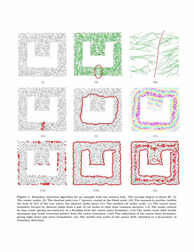
1. Flood the network from an arbitrary node, r. Eachnode records the minimum hop count to r. This im-plicitly builds a shortest path tree rooted at r. Wegenerally prefer to select r as a node on the outerboundary of the sensor field.

2. Determine the nodes that form the cut, where theshortest paths of distinct homotopy type meet afterpassing around holes. Informally, the nodes of a branchof the cut have their least common ancestor (LCA)relatively far away and their paths to the LCA wellseparated. See Figure 1(ii-iv). If there are multiplebranches of the cut, corresponding to multiple holes,delete nodes on branches of the cut in order to mergeholes, until there is only one composite hole left in thesensor field.

3. Determine a shortest cycle, R, enclosing the compos-ite hole; R serves as a coarse inner boundary. SeeFigure 1(v).

4. Flood the network from the cycle R. Each node inthe network records its minimum hop count to R. SeeFigure 1(vi).

5. Detect “extremal nodes” whose hop counts to R arelocally maximal. See Figure 1(vii).

6. Refine the coarse inner boundary R to provide tightinner and outer boundaries. These boundaries are infact cycles of shortest paths connecting adjacent ex-tremal nodes. See Figure 1(viii).

7. Undelete the nodes of the removed cut branches andrestore the real inner boundary locally.

8. At this stage we have a set of cycles corresponding tothe boundaries of the inner holes and the outer bound-ary. As a byproduct, we can compute the medial axisof the sensor field. See Figure 1(ix).

2.1 Build a shortest path treeThe first step of the algorithm is to flood the network

from an arbitrary root node r. For example, we can select rto be the node with smallest ID. This can be performed ina distributed fashion as follows. First, each sensor node psets a timer with a random remaining time. Ties are brokenby the unique IDs of the sensor nodes. When the timerof p reaches 0, the node p will begin to flood the networkand build a shortest path tree T (p). The message sent outby p contains the ID of p and the initial timer p chooses.The tree with a timer of minimum value starts first andsuppresses the construction of other trees. When the frontierof T (p) encounters a node q, there are two cases: (i) If qdoes not belong to any other tree, then q is included in thetree T (p) and q will broadcast the packet; or, (ii) If q isalready included in another tree T (p′), then the start timeof T (p) and T (p′) are compared. Only when the start timeof T (p) is earlier than that of T (p′) will the message from pbe broadcast. Eventually the tree with earliest starting timewill dominate and suppress the construction of other trees,and the packet from the node with minimum initial timerwill cover the whole network. Each node in the networkrecords the minimum hop count from this root. We denoteby T the shortest path tree constructed.

When the network size is unknown, the flooding step pro-vides a good approximation to the network diameter. By tri-angle inequality, the diameter of the network is at most 2d,where d is the distance between the root r and the deepestnode in T . d can be used to generate a reasonable thresholdfor the minimum size of the holes we aim to discover.

2.2 Find cuts in the shortest path treeHints about the presence of holes are hidden in the struc-

ture of the shortest path tree T . The “flow” of T forks neara hole, continues along opposite sides of the hole and thenmeets again past the hole. We detect where the shortestpaths meet and denote those nodes as “cut” nodes (e.g.,the red nodes in Figure 1(iv)). Nodes of the cut form cutbranches and cut vertices, where three or more cut branchescome together; cut branches are the discrete analogue ofbisectors in the (continuous) “shortest path map” and cutvertices are the discrete “SPM-vertices”; see Section 3. Fig-ure 3 shows the tree T for a network with 3 holes. In thiscase, we detect 3 groups of cut nodes (3 cut branches). Ingeneral, as will be proved later in the continuous case, if thesensor field has k interior holes and m cut vertices, there areexactly k + m cut branches in the network.

(i) (ii) (iii)

(iv) (v) (vi)

(vii) (viii) (ix)

Figure 1: Boundary detection algorithm for an example with one concave hole. The average degree is about 20. (i)

The sensor nodes; (ii) The shortest path tree T (green), rooted at the black node; (iii) The zoomed-in portion (within

the loop of (ii)) of the tree where the shortest paths meet; (iv) The marked cut nodes (red); (v) The course inner

boundary formed by shortest paths from a pair of cut nodes to their least common ancestor; (vi) The nodes colored

by hop count (giving iso-contours) in a flooding from the coarse inner boundary; (vii) The nodes (red) with locally

maximum hop count (extremal points) from the coarse boundary; (viii) The refinement of the coarse inner boundary,

giving tight inner and outer boundaries; (ix) The medial axis nodes of the sensor field, obtained as a by-product of

boundary detection.

Intuitively, the nodes in a cut are the neighboring pairs,(p, q), in the communication graph whose least common an-cestor, LCA(p, q), in the shortest path tree T is “far” fromp and q, with paths from LCA(p, q) to p and to q “wellseparated.” More formally,

Definition 1. A cut pair (p, q) is a pair of neighboringnodes in the network satisfying the following conditions: (i)The (hop) distance between p or q and y =LCA(p, q) is abovea threshold δ1; and, (ii) The maximum (hop) distance be-tween a node on the path in T from p to y and the path inT from q to y is above a threshold δ2 (See Figure 2). Thecut is the union of nodes that belong to a cut pair. Eachconnected component of the cut is a subgraph which, whenthinned, is a cut tree; the nodes of degree greater than 2 inthis tree are cut vertices, and the paths of degree-2 vertices,and their neighboring (non-cut-vertex) cut nodes, form thecut branches.

q≥ δ2

≥ δ1

cut pair

y=LCA r

p

Figure 2: Definition of a cut pair (p, q).

The two parameters in the definition of a cut pair, δ1 andδ2, specify the minimum size of the holes we want to detect.Typically, we choose them as some constant fraction of thediameter of the sensor field (e.g., experiments reported inthis paper use δ1 = δ2 = 0.18d). The condition on whethera node belongs to a cut can be checked locally. Alstrupet al. gave a distributed algorithm to compute the LCA [1].The idea is to label the nodes of a rooted tree with O(log n)bits such that by using only the labels of two nodes one cancalculate the label of their LCA. With this labeling, eachpair of neighbors in the network check for their commonancestors. If the LCA is more than distance δ1 away, wecheck if two shortest paths from these two neighbor nodesto their LCA satisfy the second condition in the definitionabove. This can be implemented by a local flooding fromeach node in the cut pair up to distance δ2. Nodes thatsatisfy both conditions mark themselves as being in the cut.

The nodes in the cut will then connect themselves intoconnected components. Furthermore, each connected com-ponent agrees on the node closest to the root (ties are brokenby the smaller ID). Specifically, each node u in the cut keepsits current knowledge of the ID of the node with smallest dis-tance to the root. If a cut node u receives a message fromits neighboring cut node about a closer node, u updatesits knowledge and sends the change to its neighboring cutnodes. Eventually, the cut nodes connect themselves intoconnected components with each cut identified by the ID ofthe closest node. If there is no hole in the network, there willbe no cut, then no connected components correspondingly.By simulation we find that this algorithm correctly finds allthe cuts when the sensor field has a reasonable density (e.g.,when the average degree is about 7 or more).

When there are multiple holes and multiple cuts in thenetwork, we artificially merge the holes by removing nodeson cut branches, until there is only one composite hole left.As will be clear later, the real boundary cycles can be easily

Figure 3: The cut pairs in a multi-hole example. 4050

nodes and the average degree is 10.

restored by undeleting the removed cut nodes. We removeall of the nodes on cut branches except the one branch fur-thest away from the root. The interior holes either connectto themselves or connect to the outer boundary. Thus, themulti-hole case is turned into a single hole scenario; thus, inthe following steps we focus on the single hole case.

2.3 Detect a coarse inner boundaryWith the cut nodes detected, we would like to find a

coarse inner boundary R that encloses the (composite) inte-rior hole. R is then refined to provide tight inner and outerboundaries.

Definition 2. A coarse inner boundary R is a shortestcycle enclosing the interior hole in the sensor field.

Recall that we have turned any multi-hole sensor fieldinto a single composite hole sensor field by removing all cutbranches except one. All the nodes in the unique cut branchhave the ID of the node closest to the root. Thus, the closestnode p, together with its partner q in the cut pair, will findthe shortest paths between them that do not go throughany cut node. This can be implemented in two ways. Anobvious way is to use any shortest path algorithm to findthis path. In order to prevent the path from going throughany cut nodes, we remove all the edges between cut pairs.Alternatively, we can use the two shortest paths from p andq to LCA(p, q). Together with the edge pq, we obtain a cy-cle that encloses the hole. This cycle is not necessarily theshortest cycle. But we can greedily shrink it to be as tightas possible, by the following k-hop shrinking process. Forany two nodes that are within k hops on the cycle, we checkwhether there exists a shorter path between these two nodes.If so, we use the shorter path to replace the original segmenton the cycle and shorten the total length. For example, a 2-hop shrinking checks, for every three adjacent nodes on thecycle, say x, y, z, whether (x, z) is an edge. If so, we shrinkthe cycle by excluding y. In a sensor field with reasonabledensity, the greedy process stops at the shortest cycle so thatno more improvement is made. For a sensor field with onlyone convex shape hole, the coarse inner boundary actuallyis the real inner boundary, as in Figure 4(i). If the graph

has a concave hole (Figure 1(v)), the coarse inner bound-ary R will be a shortest circuit containing this concave holeand, thus, approximates its convex hull. A multi-hole ex-ample is shown in Figure 4(ii). Notice that this coarse innerboundary provides a consistent ordering of the nodes on thiscycle.

We note that the shortest paths from a cut pair to theirLCA do not go through any cut nodes, as proved later (Sec-tion 3). Thus, the removal of cut nodes in a multi-hole sce-nario is not a problem for the discovery of the coarse innerboundary by the greedy shrinking scheme.

(i) (ii)

Figure 4: The coarse inner boundary for (i) a convex

hole scenario; (ii) a multi-hole scenario with all but one

cut branch removed, one interior hole connected to the

outer boundary.

2.4 Find extremal nodesThe coarse inner boundary R is not tight in the case of a

concave hole. Also, we have no idea about the outer bound-ary. Next, we refine the coarse inner boundary to providetight cycles for both inner and outer boundaries. This re-finement is through finding what are called “extremal nodes”with respect to R.

Definition 3. An extremal node is a node whose mini-mum hop count to nodes in R is locally maximal.

To discover extremal nodes, we have the nodes on R syn-chronize among themselves and start to flood the networkat roughly the same time [5] [12]. Each node in the networkrecords the minimum hop count to nodes in the coarse innerboundary R. This is as if we merge the nodes in R to adummy root σ, and build a shortest path tree T (σ), rootedat σ for the whole network. The extremal nodes are theones with locally maximum distance to R. Each extremalnode can detect itself by checking its direct neighbors. In-tuitively, the extremal nodes are on the outer boundary orare the ridges on the real inner boundary of a concave hole(Figure 1(vii)).

With the extremal nodes identified, we also need to knowtheir relative orderings to connect them to a consistent bound-ary. This ordering can be derived from the ordering of thenodes on R. Specifically, for each node on R, we assign alabel in [0, L] that indicates its position on R. A node u thatis k hops away from R may have multiple neighbors (k − 1)hops away from R. Thus, the label of u, `(u), is taken as theaverage of the labels of all of its neighbors that are (k − 1)hops away from R. Each node in the network records the

distance to R as well as its label. The relative ordering ofextremal nodes is decided by their labels.

When there are many extremal nodes and some of themhave similar labels, we would like to eliminate some of themand take a few representative nodes for the next step. Thegoal for this clean-up is to take sampled extremal nodes sothat we can easily sort them. We first find the connectedcomponents for all extremal nodes, denoted as extremal con-nected components (ECC). These can be done with the samedistributed strategy as used to find connected componentsfor the cuts. Next, we select at most two nodes as the rep-resentatives for each ECC (an ECC may contain only onenode). These two nodes have the greatest distance betweenthem in their affiliated ECC. These nodes will be connectedaccording to their labels to refine inner and outer bound-aries.

2.5 Find the outer boundary and refine thecoarse inner boundary

With the extremal nodes and a linear ordering of them,we would like to connect them into a cycle consistent withthis ordering. Notice that here we only consider the casewith one inner hole, since we have removed the cuts to con-nect multiple holes into a composite hole. If this compositehole is convex, then all extremal nodes belong to the outerboundary. If the composite hole is concave, as in the multi-hole case, there will be two types of extremal nodes, thoseon the outer boundary and those on the interior of R. Weuse the following rule to differentiate extremal nodes on dif-ferent sides of R.

The removal of R, together with all of the 1-hop neighborsof R, partitions the network into several connected compo-nents Ci, i = 1, . . . , w. Now we would like to connect theextremal points into extremal paths in each connected com-ponent, which will then be further connected into boundarycycles. We first focus on a particular connected componentand describe how an extremal path is constructed. Specif-ically, all of the nodes that are 2 hops away from R willconnect themselves through local flooding. This results in apath (or a cycle) Pj with a corresponding maximum indexand minimum index along R. Now we would like to refinethis path Pj so as to force it to go through the extremalnodes in this connected component as well as the two nodeson Pj with maximum and minimum indexing. Notice thateach extremal node has shortest paths from some nodes onR. Now we connect two extremal nodes with adjacent order-ing by the shortest path between them. To find the shortestpath between two extremal points, again we can either useany shortest path algorithm or a greedy approach. For thelatter, we notice that there is a natural path between anytwo extremal nodes u, v, composed by the shortest path fromu to its closest point on Pj , the shortest path from v to itsclosest point on Pj and a segment of Pj between the corre-spondences of u, v. The shortest paths from extremal pointsto Pj can be found by following the parent pointer towardsR (in the tree T (σ)). Then, we can greedily refine this pathand find the shortest path between u and v.

By the above procedure, the extremal nodes are connectedinto a path Pj , in each connected component. If one ofthe paths is actually a cycle, then it is already a boundarycycle. If there are paths that are not connected into cycles,then we tour the coarse boundary R and connect them intoboundary cycles. In particular, we start from anywhere on

R and tour along R; when there is a neighboring node (in2 hops) who is on an extremal path Pj , then we branchon Pj . This will eventually come back and close a cycle.Then, we tour R again, from a node that is not on thefirst cycle, and branch on extremal paths as long as we can.This will generate another cycle. So far, we classify extremalnodes and connect them into two cycles, corresponding tothe inner and outer boundary. Figure 5 shows the resultsfor two examples after this stage.

(i) (ii)

Figure 5: The outer boundary and the refined inner

boundary. (i) 2-hole example; (ii) multi-hole example.

As will be shown in Section 3, in the continuous case all ofthe boundary points are identified as extremal points. How-ever, in a discrete network, the shortest path is computed ona combinatorial graph. Thus, not all of the boundary nodesare identified as extremal nodes. The boundary refinementcan be performed in an iterative fashion such that we floodfrom the current boundary cycle and identify more extremalpoints until the boundary cycle is sufficiently tight.

2.6 Restore the inner boundaryThe final step of our method is to recover the inner holes

in the sensor field and find their boundaries. We undeletethe cut nodes we removed earlier and restore the correctinner boundary. For each cut, we find a cut pair (p, q) suchthat the inclusion of edge pq in the refined inner boundaryR partitions the inner boundary into two boundary cycles.If p, q are by themselves not on the refined inner boundaryR, then we do a local search from p, q to discover nodeson R. The two new boundary cycles will share nodes p, q.Then, we shrink the cycles locally to make them tight. Here,the shrinking procedure has a restriction that the shrunkpath still has to pass through the extremal nodes. Thus, wepartition the refined inner boundary into a number of cycles,each representing the boundary of an inner hole. Figure 6shows our final results for two examples.

2.7 The medial axis of the sensor fieldThe boundaries of the sensor field capture the global geo-

metric shape information, and thus can be used to generateother structures related to the global geometry. For exam-ple, we can define the quasi-Voronoi diagram for the bound-aries such that sensor nodes are classified by their closestboundary. In another example, we can compute the medialaxis of the sensor field. The medial axis is defined as theset of nodes with at least two closest boundary nodes2. The

2Since hop counts are discrete, we allow a node on the medialaxis with two closest boundary nodes that differ by 1 in hopcount.

(i) (ii)

Figure 6: The boundary cycles created by the connec-

tion of nodes: (i) 2-hole example; (ii) multi-hole example.

medial axis can be used to generate virtual coordinates forefficient greedy routing [3]. Both the quasi-Voronoi diagramand the medial axis can be discovered by a simple floodingfrom the boundary cycles. Figure 7 shows the results for our3-hole face example.

With our boundary information, we start from all bound-ary nodes and flood the network simultaneously. Each nodethus records its closest boundary. All of the nodes withthe same closest boundary are naturally classified to be inthe same cell of the quasi-Voronoi diagram. Further, thenodes at which the frontiers collide belong to the medialaxis. Specifically, the detection of nodes on the medial axiscan be done locally. Denote the boundary cycles by Ri,i = 1, . . . , k. During the flooding from the boundaries, eachnode in the boundary sends out a packet containing theboundary containing it, its position based on the originatorboundary, and the number of hops this packet has traveled,as denoted by a tuple (i, `i(v), hi(v)). A node, upon receiv-ing a packet (i, `i(v), hi(v)), does one of the following things.If a node has not received earlier packets with smaller hopcounts to boundaries, it records (i, `i(v), hi(v)), where hi(v)is the minimum hop count distance to the originator of thepacket, drops earlier tuples with larger hop counts, and re-transmits the packet. In the end, each node only containsthe tuples with the minimum hop count distance. Thereare three possible cases: (1). Only one minimum hop counttuple is left for the node, so the node is not a medial axisnode. (2). More than one minimum hop count tuple is left,and these tuples are generated by different boundary cycles,which means the node has more than one closest boundarynode, so the node is on the medial axis. (3). More thanone minimum hop count tuple is left, and these tuples aregenerated by the same boundary cycle, so we need to com-pare the ` values in these tuples; if they differ a lot, thenthe node is on the medial axis. This case corresponds to aninward convex (reflex) segment in the boundary.

3. PROOF OF CORRECTNESS IN THECONTINUOUS CASE

In this section we prove rigorously that the algorithm willcorrectly detect all the inner and outer boundaries in a con-tinuous domain with polygonal boundaries. (The resultsapply also to non-polygonal domains, since they are approx-imated by polygons.) Let F be a closed polygonal domainin the plane, with k simple polygonal obstacles inside; F is asimple polygon P , minus k disjoint polygonal holes. We refer

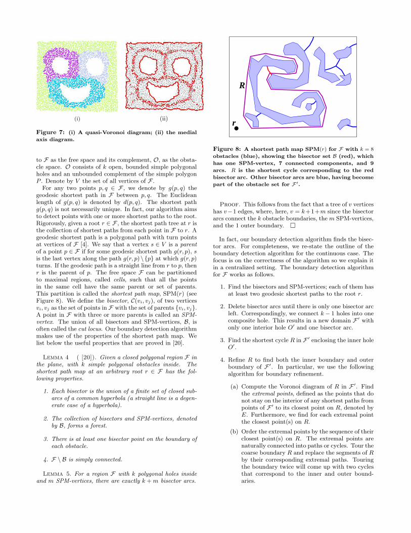
(i) (ii)

Figure 7: (i) A quasi-Voronoi diagram; (ii) the medial

axis diagram.

to F as the free space and its complement, O, as the obsta-cle space. O consists of k open, bounded simple polygonalholes and an unbounded complement of the simple polygonP . Denote by V the set of all vertices of F .

For any two points p, q ∈ F , we denote by g(p, q) thegeodesic shortest path in F between p, q. The Euclideanlength of g(p, q) is denoted by d(p, q). The shortest pathg(p, q) is not necessarily unique. In fact, our algorithm aimsto detect points with one or more shortest paths to the root.Rigorously, given a root r ∈ F , the shortest path tree at r isthe collection of shortest paths from each point in F to r. Ageodesic shortest path is a polygonal path with turn pointsat vertices of F [4]. We say that a vertex s ∈ V is a parentof a point p ∈ F if for some geodesic shortest path g(r, p), sis the last vertex along the path g(r, p)\{p} at which g(r, p)turns. If the geodesic path is a straight line from r to p, thenr is the parent of p. The free space F can be partitionedto maximal regions, called cells, such that all the pointsin the same cell have the same parent or set of parents.This partition is called the shortest path map, SPM(r) (seeFigure 8). We define the bisector, C(vi, vj), of two verticesvi, vj as the set of points in F with the set of parents {vi, vj}.A point in F with three or more parents is called an SPM-vertex. The union of all bisectors and SPM-vertices, B, isoften called the cut locus. Our boundary detection algorithmmakes use of the properties of the shortest path map. Welist below the useful properties that are proved in [20].

Lemma 4 ( [20]). Given a closed polygonal region F inthe plane, with k simple polygonal obstacles inside. Theshortest path map at an arbitrary root r ∈ F has the fol-lowing properties.

1. Each bisector is the union of a finite set of closed sub-arcs of a common hyperbola (a straight line is a degen-erate case of a hyperbola).

2. The collection of bisectors and SPM-vertices, denotedby B, forms a forest.

3. There is at least one bisector point on the boundary ofeach obstacle.

4. F \ B is simply connected.

Lemma 5. For a region F with k polygonal holes insideand m SPM-vertices, there are exactly k + m bisector arcs.

r

R

Figure 8: A shortest path map SPM(r) for F with k = 8

obstacles (blue), showing the bisector set B (red), which

has one SPM-vertex, 7 connected components, and 9

arcs. R is the shortest cycle corresponding to the red

bisector arc. Other bisector arcs are blue, having become

part of the obstacle set for F ′.

Proof. This follows from the fact that a tree of v verticeshas v−1 edges, where, here, v = k+1+m since the bisectorarcs connect the k obstacle boundaries, the m SPM-vertices,and the 1 outer boundary.

In fact, our boundary detection algorithm finds the bisec-tor arcs. For completeness, we re-state the outline of theboundary detection algorithm for the continuous case. Thefocus is on the correctness of the algorithm so we explain itin a centralized setting. The boundary detection algorithmfor F works as follows.

1. Find the bisectors and SPM-vertices; each of them hasat least two geodesic shortest paths to the root r.

2. Delete bisector arcs until there is only one bisector arcleft. Correspondingly, we connect k − 1 holes into onecomposite hole. This results in a new domain F ′ withonly one interior hole O′ and one bisector arc.

3. Find the shortest cycle R in F ′ enclosing the inner holeO′.

4. Refine R to find both the inner boundary and outerboundary of F ′. In particular, we use the followingalgorithm for boundary refinement.

(a) Compute the Voronoi diagram of R in F ′. Findthe extremal points, defined as the points that donot stay on the interior of any shortest paths frompoints of F ′ to its closest point on R, denoted byE. Furthermore, we find for each extremal pointthe closest point(s) on R.

(b) Order the extremal points by the sequence of theirclosest point(s) on R. The extremal points arenaturally connected into paths or cycles. Tour thecoarse boundary R and replace the segments of Rby their corresponding extremal paths. Touringthe boundary twice will come up with two cyclesthat correspond to the inner and outer bound-aries.

5. Undelete the removed bisector arcs. Restore the bound-aries of interior holes and the outer boundary.

Next we will prove that this algorithm correctly finds allthe boundaries of F . The proof consists of a number oflemmas.

Lemma 6. The domain F ′ has one interior polygonal hole.

Proof. This is due to the fact in Lemma 4 that F \B issimply connected. Thus, by removing all but one bisectorarc and all SPM-vertices, we obtain a polygonal region F ′

with one interior hole.

Now we focus on F ′ and argue that we indeed find thecorrect outer and inner boundaries of F ′ by the iterativerefinement. We only prove for the outer boundary R+; thecorrectness of the inner boundary R− can be proved in thesame way. By the refinement algorithm, we can find theVoronoi diagram of R by a wavefront propagation algorithm(e.g., [15]). The extremal points are the points that do notstay on the interior of any shortest paths from points of F ′

to its closest point on R. Due to the properties of wave-front propagation, the extremal points must be either onthe boundary or on the medial axis, where wavefronts col-lide [16,20]. However, since cycle R is a shortest path cyclesurrounding the hole, we argue that the extremal points onthe exterior of R must stay on the boundary of F ′.

Lemma 7. The extremal points are exactly the boundarypoints of F ′.

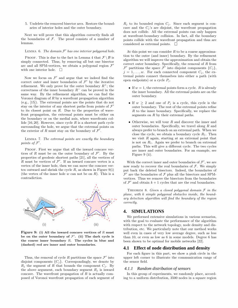
Proof. First we argue that all the inward concave ver-tices of R must be on the outer boundary of F ′. By theproperties of geodesic shortest paths [21], all the vertices ofR must be vertices of F ′. If an inward concave vertex is avertex of the inner hole, then we can move the concave ver-tex outward and shrink the cycle R, as shown in Figure 9(i)(the vertex of the inner hole w can not be on R). This is acontradiction.

�������������������������

�������������������������

�������������������������������������������������

�������������������������������������������������

������������������������������������������

���������������������������������������������������������������������������������������������������������

���������������������������������������������������������������

����������������������������

����������������������������

vR

Cj

w

u

(i) (ii)

Figure 9: (i) All the inward concave vertices of R must

be on the outer boundary of F ′. (ii) The dark cycle is

the coarse inner boundary R. The cycles in blue and

(dashed) red are inner and outer boundaries.

Thus, the removal of cycle R partitions the space F ′ intodisjoint components {Cj}. Correspondingly, we denote byRj the segment of R that bounds the component Cj . Bythe above argument, each boundary segment Rj is inwardconcave. The wavefront propagation of R is actually com-posed of Voronoi wavefront propagation of each segment of

Rj to its bounded region Cj . Since each segment is con-cave and the Cj ’s are disjoint, the wavefront propagationdoes not collide. All the extremal points can only happenat wavefront-boundary collision. In fact, all the boundarypoints collide with the wavefront propagation and thus areconsidered as extremal points.

At this point we can consider R to be a coarse approxima-tion to the outer (and inner) boundary. By the refinementalgorithm we will improve the approximation and obtain thecorrect outer boundary. Specifically, the removal of R fromF ′ partitions the space F ′ into disjoint components {Cj},j = 1, . . . , w. For each connected component Cj , the ex-tremal points connect themselves into either a path (withopen endpoints) or a cycle Pj .

• If w = 1, the extremal points form a cycle. R is alreadythe inner boundary. All the extremal points are on theouter boundary.

• If w ≥ 2 and one of Pj is a cycle, this cycle is theouter boundary. The rest of the extremal points refineR to the inner boundary. Specifically, we replace thesegments on R by their extremal paths.

• Otherwise, we will tour R and discover the inner andouter boundaries. Specifically, we travel along R andalways prefer to branch on an extremal path. When weclose the cycle, we obtain a boundary cycle R1. Thenwe visit R again, starting at an extremal point thatis not on R1. Again we prefer to branch on extremalpaths. This will give a different cycle. The two cyclesare inner and outer boundaries. For an example, seeFigure 9 (ii).

With the correct inner and outer boundaries of F ′, we arenow ready to recover the real boundaries of F . We simplyput back the deleted bisectors. Indeed, the boundaries ofF ′ are the boundaries of F plus all the bisectors and SPM-vertices. Thus we remove the bisectors from the boundariesof F ′ and obtain k + 1 cycles that are the real boundaries.

Theorem 8. Given a closed polygonal domain F in theplane, with k simple polygonal obstacles inside, the bound-ary detection algorithm will find the boundary of the regioncorrectly.

4. SIMULATIONSWe performed extensive simulations in various scenarios,

with the goal to evaluate the performance of the algorithmwith respect to the network topology, node density and dis-tribution, etc. We particularly note that our method workswell even in cases of very low average degree, such as lessthan 10, or even as low as 6 in some models. Degree 6 hasbeen shown to be optimal for mobile networks [22].

4.1 Effect of node distribution and densityFor each figure in this part, we show a pink circle in the

upper left corner to illustrate the communication range ofthe sensor field.

4.1.1 Random distribution of sensorsIn this group of experiments, we randomly place, accord-

ing to a uniform distribution, 3500 nodes in a square region

with one hole. The average degree of the graph is variedby adjusting the communication radius. Figure 10 showsthe results using our method. As expected, as the averagedegree of the network increases, the performance of the al-gorithm improves.

The unsatisfactory result in Figure 10(i) is due to insuf-ficient connectivity. The average degree is 7; however, therandom distribution tends to have clustered nodes and holes.Thus, in sparse regions some nodes are incorrectly judged tobe extremal, and the final outer boundary is then requiredto pass through these mistaken extremal nodes. When theaverage degree reaches 10, the communication graph is bet-ter connected, and the results improve.

For comparison, SHAWN [19] did not find a starting so-lution (a “flower”) for cases (i) and (ii); it found apparentlycorrect boundaries for cases (iii) and (iv), indistinguishablefrom our results. The method of Funke and Klein [11] haddifficulty with all 4 cases; see Figure 11(i), (ii).

Connectivity is necessary for computing the shortest pathtree and determining cuts, etc. In fact, this low-degree graphwith insufficient connectivity is the major troubling issue forprior boundary detection methods. Since our method onlyrequires the communication graph, we can apply some sim-ple strategies to increase artificially the average degree. Fora disconnected network, we use the largest connected com-ponent of the graph to build our shortest path tree. Thenwe artificially enlarge the communication radius by taking 2-hop/3-hop neighbors as “fake” 1-hop neighbors. In this way,the connectivity of the graph will be ameliorated and the re-sults will be improved correspondingly. Figure 12 shows theimprovement by this simple strategy. The result using 3-hopneighbors has fewer incorrectly marked extremal nodes, andthe final boundary is in good shape except that the bound-ary cycle is not very tight. This is understandable since wemake the communication range artificially larger, so thatmore nodes are “on” the boundary now.

4.1.2 Grid with random perturbationIn this simulation, we put about 3500 nodes on a grid and

then perturbed each point by a random shift. In particular,for each original grid node we create two random numbersmodulo the length and the width of each block of the grid,the use these two small numbers to perturb the positions ofthe nodes. This distribution may be a good approximationof manual deployments of sensors; it also gives an alternativemeans of modeling “uniform” distributions, while avoidingclusters and “holes” that can arise from the usual continuousuniform distribution or Poisson process. Refer to Figure 13.Our method gives very good results for graphs with averagedegree 6 or more.

SHAWN [19] found good boundaries for (ii)-(iii), but didnot find a starting solution for (i). The method of Funkeand Klein [11] did well for case (iii) but less well for thelower degree cases; see Figure 11(iii).

4.1.3 Low density, sparse graphsIn this group of experiments (Figure 14), we scatter nodes

in a square region with one hole. In order to guaranteegood connectivity, the nodes are distributed on a randomlyperturbed grid. The leftmost image of Figure 14 has about3500 nodes; then, from left to right, each example has about1000 fewer nodes, becoming more and more sparse. Ourexperiments show that if we fix the communication radius,

and decrease the density of nodes, our method performs well,even for low density or sparse graphs (Figure 14(iv)), as longas the average degree is at about 7 or more.

SHAWN [19] did not find a starting solution for case (iv);it found good boundaries for cases (i)-(iii). The method ofFunke and Klein [11] also performs well in cases (i)-(iii),but it performs less well in the lowest-degree case (iv); seeFigure 11(iv).

4.2 Further examplesIn Figure 15, we illustrate more results for a variety of

more intricate geometries, including a spiral shape, a floor-plan, etc.

5. DISCUSSIONWhile our new boundary detection algorithm provably

finds boundaries in the continuous case (Section 3), in dis-crete sensors networks several implementation issues arise.

First, even for a given homotopy type, there need notbe a unique shortest path between two nodes. Thus, theboundary cycle discovered by our algorithm, as shown in thesimulations, may not tightly surround the real boundaries.Currently, we have two approaches to improve it. One is tomake use of the fact that the nodes with lower degree aremore likely to be on the boundary; thus, we implementeda preferential scheme for low-degree nodes when comput-ing shortest paths. Another approach is to use an iterativemethod to find more extremal nodes, and then refine theboundary; this can also help to address the issue that sev-eral extremal points may have the same positions becausewe use hop counts to approximate true distances.

Second, deciding the correct orderings of the extremalnodes requires some care. In the continuous case, extremalnodes project to their nearest node in the rough inner bound-ary, resulting in a consistent ordering of extremal nodes, asshown in Section 3. In the discrete case, since we use hopcount to approximate the true distance, it is possible thatdifferent extremal points are mapped to the same position onthe inner boundary, obscuring their ordering. Again, by us-ing an iterative procedure, we delete all the extremal nodeswith duplicate positions except one and then iteratively findmore extremal points and refine the boundary gradually.

In practice, the sensor nodes often know some partial lo-cation information or relative angular information. Suchpositional information can help to improve the performanceof our boundary detection algorithm. For example, if thenodes have knowledge of a universal north direction, it iseasier to distinguish the extremal nodes in the interior andexterior of rough boundary. Also, if we have estimated dis-tance or other rough localization information, other thanpure hop count, the procedure to find shortest paths willbecome more reliable.

Finally, our method discussed until now assumes a sensorfield with holes. We remark that the case with no holes canbe solved as well. If a network has no hole, we discover thisfact, since the network has no cut. In addition, the roughinner boundary degenerates to the root node. Then, we candiscover the extremal nodes and connect them to find theouter boundary.

Acknowledgements. We thank Stefan Funke and Alexan-der Kroller for running comparison experiments with theiralgorithms on our data. We thank the reviewers for numer-ous helpful suggestions that improved the presentation.

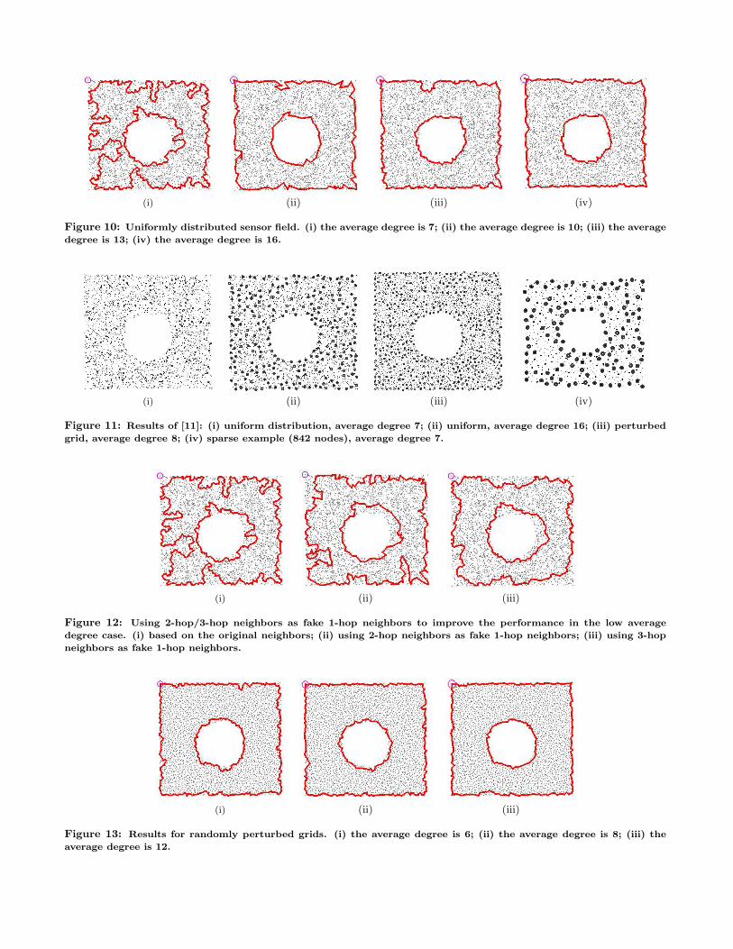
(i) (ii) (iii) (iv)

Figure 10: Uniformly distributed sensor field. (i) the average degree is 7; (ii) the average degree is 10; (iii) the average

degree is 13; (iv) the average degree is 16.

(i) (ii) (iii) (iv)

Figure 11: Results of [11]: (i) uniform distribution, average degree 7; (ii) uniform, average degree 16; (iii) perturbed

grid, average degree 8; (iv) sparse example (842 nodes), average degree 7.

(i) (ii) (iii)

Figure 12: Using 2-hop/3-hop neighbors as fake 1-hop neighbors to improve the performance in the low average

degree case. (i) based on the original neighbors; (ii) using 2-hop neighbors as fake 1-hop neighbors; (iii) using 3-hop

neighbors as fake 1-hop neighbors.

(i) (ii) (iii)

Figure 13: Results for randomly perturbed grids. (i) the average degree is 6; (ii) the average degree is 8; (iii) the

average degree is 12.

(i) (ii) (iii) (iv)

Figure 14: Results when the density of the graph decreases. (i) 3443 nodes and the average degree is 35; (ii) 2628

nodes and the average degree is 25; (iii) 1742 nodes and the average degree is 16; (iv) 842 nodes and the average

degree is 7.

(i) (ii) (iii) (iv)

Figure 15: Results for more interesting examples. (i) A spiral shape with 5040 nodes and the average degree is 21;

(ii) A building floor shape with 3420 nodes and the average degree is 20; (iii) A cubicle shape in an office with 6833

nodes and the average degree is 17; (iv) A double star shape with 2350 nodes and the average degree is 17.

6. REFERENCES[1] S. Alstrup, C. Gavoille, H. Kaplan, and T. Rauhe. Nearest

common ancestors: a survey and a new distributed algorithm.In Proc. 14th ACM Sympos. Parallel Algorithms andArchitectures, pp. 258–264, 2002.

[2] P. Bose, P. Morin, I. Stojmenovic, and J. Urrutia. Routingwith guaranteed delivery in ad hoc wireless networks. WirelessNetworks, 7(6):609–616, 2001.

[3] J. Bruck, J. Gao, and A. Jiang. MAP: Medial axis basedgeometric routing in sensor networks. In Proc. ACM/IEEEInternat. Conf. on Mobile Computing and Networking(MobiCom), pp. 88–102, 2005.

[4] M. de Berg, M. van Kreveld, M. Overmars, andO. Schwarzkopf. Computational Geometry: Algorithms andApplications. Springer-Verlag, Berlin, 1997.

[5] J. Elson. Time Synchronization in Wireless Sensor Networks.PhD thesis, University of California, Los Angeles, May 2003.

[6] Q. Fang, J. Gao, and L. Guibas. Locating and bypassingrouting holes in sensor networks. In Proc. Mobile Networksand Applications, vol. 11, pp. 187–200, 2006.

[7] Q. Fang, J. Gao, L. Guibas, V. de Silva, and L. Zhang.GLIDER: Gradient landmark-based distributed routing forsensor networks. In Proc. 24th Conference of the IEEECommunication Society (INFOCOM), pp. 339–350, 2005.

[8] S. P. Fekete, M. Kaufmann, A. Kroller, and N. Lehmann. Anew approach for boundary recognition in geometric sensornetworks. In Proc. 17th Canadian Conference onComputational Geometry, pp. 82–85, 2005.

[9] S. P. Fekete, A. Kroller, D. Pfisterer, S. Fischer, andC. Buschmann. Neighborhood-based topology recognition insensor networks. In Proc. ALGOSENSORS, Springer LNCSvol. 3121, pp. 123–136, 2004.

[10] S. Funke. Topological hole detection in wireless sensornetworks and its applications. In Proc. Joint Workshop onFoundations of Mobile Computing, pp. 44–53, 2005.

[11] S. Funke and C. Klein. Hole detection or: “How muchgeometry hides in connectivity?”. In Proc. 22nd ACMSympos. Computational Geometry, pp. 377–385, 2006.

[12] S. Ganeriwal, R. Kumar, and M. B. Srivastava. Timing-syncprotocol for sensor networks. In Proc. 1st Internat. Conf. onEmbedded Networked Sensor Systems, pp. 138–149, 2003.

[13] D. Ganesan, B. Krishnamachari, A. Woo, D. Culler, D. Estrin,and S. Wicker. Complex behavior at scale: An experimentalstudy of low-power wireless sensor networks. UCLA/CSD-TR02-0013, UCLA, 2002.

[14] R. Ghrist and A. Muhammad. Coverage and hole-detection insensor networks via homology. In Proc. 4th Internat. Sympos.Information Processing in Sensor Networks, pp. 254–260,2005.

[15] M. Held. Voronoi diagrams and offset curves of curvilinearpolygons. Computer Aided Design, 30(4):287–300, 1998.

[16] J. Hershberger and S. Suri. An optimal algorithm forEuclidean shortest paths in the plane. SIAM Journal onComputing, 28(6):2215–2256, 1999.

[17] B. Karp and H. Kung. GPSR: Greedy perimeter statelessrouting for wireless networks. In Proc. ACM/IEEE Internat.Conf. on Mobile Computing and Networking, pp. 243–254,2000.

[18] Y.-J. Kim, R. Govindan, B. Karp, and S. Shenker. Geographicrouting made practical. In Proc. 2nd USENIX/ACM Sympos.Networked System Design and Implementation, pp. 217–230,2005.

[19] A. Kroller, S. P. Fekete, D. Pfisterer, and S. Fischer.Deterministic boundary recognition and topology extractionfor large sensor networks. In Proc. 17th ACM-SIAM Sympos.Discrete Algorithms, pp. 1000–1009, 2006.

[20] J. S. B. Mitchell. A new algorithm for shortest paths amongobstacles in the plane. Ann. Math. Artif. Intell., 3:83–106,1991.

[21] J. S. B. Mitchell. Geometric shortest paths and networkoptimization. In J.-R. Sack and J. Urrutia, eds., Handbook ofComputational Geometry, pp. 633–701. Elsevier, 2000.

[22] E. M. Royer, P. M. Melliar-Smith, and L. E. Moser. Ananalysis of the optimum node density for ad hoc mobilenetworks. In Proc. IEEE Internat. Conf. onCommunications, pp. 857–861, 2001.