Boundary Matting for View Synthesis

Samuel W. Hasinoff a,∗, Sing Bing Kang b, and Richard Szeliski b

aDept. of Computer Science, University of Toronto, Toronto, CanadabInteractive Visual Media Group, Microsoft Research, Redmond, WA, USA

Abstract

In the last few years, new view synthesis has emerged as an important applica-tion of 3D stereo reconstruction. While the quality of stereo has improved, it is stillimperfect, and a unique depth is typically assigned to every pixel. This is problem-atic at object boundaries, where the pixel colors are mixtures of foreground andbackground colors. Interpolating views without explicitly accounting for this effectresults in objects with a “cut-out” appearance.

To produce seamless view interpolation, we propose a method called boundarymatting, which represents each occlusion boundary as a 3D curve. We show how thismethod exploits multiple views to perform fully automatic alpha matting and tosimultaneously refine stereo depths at the boundaries. The key to our approach is the3D representation of occlusion boundaries estimated to sub-pixel accuracy. Startingfrom an initial estimate derived from stereo, we optimize the curve parametersand the foreground colors near the boundaries. Our objective function maximizesconsistency with the input images, favors boundaries aligned with strong edges,and damps large perturbations of the curves. Experimental results suggest that thismethod enables high-quality view synthesis with reduced matting artifacts.

Key words: Multi-view stereo, view synthesis, image matting, occlusionboundaries, sub-pixel reconstruction, 3D curves

1 Introduction

Although stereo correspondence was one of the first problems in computervision to be extensively studied, automatically obtaining dense and accurateestimates of depth from multiple images remains a challenging problem [1].

∗ Corresponding author.Email address: hasinoff@cs.toronto.edu (Samuel W. Hasinoff).

Preprint submitted to Elsevier Science 26 October 2005

1.0 0.4 0.9 0.00.20.7

true a

resampled a

reference view synthesized view

subpixelboundary

Fig. 1. View synthesis with matting. The shaded polygon represents the foregroundobject, and the overlaid squares represent pixels. If the object is represented withan exact sub-pixel boundary model, the true distribution of α (per-pixel fractionforeground contribution) can be recovered by integration. By contrast, synthesizingnew views from a pixel-level representation requires resampling α, which can leadto blurring artifacts at object boundaries. The synthesized view corresponds to ahalf-pixel translation, resampled with linear interpolation.

Most stereo research has been concerned solely with methods for producingaccurate depth maps, so interpolated views are rarely evaluated as results.By contrast, our explicit goal is superior view synthesis from stereo. Even foreasy scenes in which all objects are opaque, diffuse, and well-textured, state-of-the-art stereo techniques often fail to generate high-quality interpolatedviews. Even if a perfect depth map were available, current methods for viewinterpolation share two major limitations:

• Sampling blur. There is an effective loss of resolution caused by resamplingand blending the input views.

• Boundary artifacts. Foreground objects seem to pop out of the scene, asin bad blue-screen composites, because most current methods do not per-form matting to resolve mixed pixels at object boundaries into their fore-ground and background components. (There are a few notable exceptions,as discussed in the next section.)

In this paper, we focus on the issue of boundary artifacts and propose atechnique we call boundary matting to reduce such artifacts. Our technique, asoutlined in Figs. 2–3, combines ideas from image matting and stereo to resolvemixed boundary pixels. Our approach consists of estimating 3D curves overmultiple views and uses stereo data to bootstrap this estimation.

The key feature of our approach is that occlusion boundaries are represented in3D. This results in several improvements over the state of the art. First, com-pared to video matting [2] and other methods that recover pixel-level mattesfor the input views [3–6], our method is theoretically better suited to viewsynthesis, because it avoids the blurring associated with resampling thosemattes (Fig. 1). Second, our method performs automatic matting from im-perfect stereo data, fully incorporating multiple views, for large-scale opaqueobjects. Third, our method exploits information from matting to refine stereodisparities along occlusion boundaries. Fourth, our method estimates occlu-

2

sion boundaries to sub-pixel accuracy, suitable for super-resolution or zooming.Fifth, our error metric is symmetric with respect to the input images, and sodoes not overly favor specific frames.

Our approach is based on several assumptions. First, we assume that the sceneis made up of opaque Lambertian surfaces, i.e., surfaces that satisfy color con-stancy across the different input views. In practice, we can handle scenes thatdeviate somewhat from this assumption, treating non-Lambertian effects nearobject boundaries as noise. Moreover, we do not consider wide-baseline stereoconfigurations where these effects are most pronounced. Another importantassumption is that the projected 2D boundaries correspond to the same 3Dedge of an object. This is strictly true only for planar objects, however, this ap-proximation is reasonable for small camera motion or relatively flat or distantobjects (see Sec. 3.1).

2 Previous work

In their seminal blue screen matting paper, Smith and Blinn [7] review tradi-tional film-based matting techniques and propose a triangulation method formatting static foreground objects using multiple images taken with differentbackgrounds (see Sec. 3). More recent matting research has focused on naturalimage matting, where the goal is to estimate the matte from a single image,given regions hand-labelled as completely foreground and background [8–12,4].These methods operate by propagating statistics of the labelled color distrib-utions throughout the unlabelled regions, yielding impressive results. Chuanget al. extend their approach from [9] using optical flow techniques to obtain asemi-automated method for matting video sequences [2]. Most recently, stereodata was used to automatically perform the initial labeling for natural imagematting, but the matting was estimated independently in each view [5].

Several researchers have also investigated an additive transparent image for-mation model, useful for separating the reflections found on glass and specularsurfaces [13,14]. Along the same lines, additive transparency has been decom-posed based on parameterizing the dominant motions in the scene [15].

There has been some work done on estimating transparency from stereo datain general terms [6,16,17]. In [6], transparency was estimated in a volumet-ric fashion along with depth, using a plane-sweep algorithm, generalized to afour-dimensional xydα search space. Results were mainly shown for syntheticproblems, but even for those, the quality of interpolated views was limited.Similarly, the iterative voxel reconstruction approach presented in [16] gaveresults unsuitable for view synthesis, whereas [17] is more appropriate for vol-umetric scenes that are semi-transparent everywhere. Mixed pixels for stereo

3

§4.2 §4.1

§4.3

§3.1

input images(composites), C

stereo depthinformation

background(clean plate), B

alpha matte, a

foreground, F

objectivefunction, O

§5

boundary

curve, q

Fig. 2. Block diagram describing the system architecture. The dashed lines indicatethat the objective function is used to optimize the parameters of the boundary curveand the foreground colors.

have also been examined as a consequence of using mixture models for esti-mating optical flow [18], and in developing matching metrics more robust tomixing [19].

Most closely related to our work is the method proposed by Wexler et al. [3],which also estimates matting by incorporating multiple views of a scene. How-ever, as described in Sec. 3, this method effectively calculates alpha in thereference view only, and therefore requires resampling the mixed pixels (i.e.,alpha values) from other views. As shown in Fig. 1, this can introduce unde-sirable blurring. Another basic limitation of this method is that high qualitystereo data is required everywhere in the image, and its performance on inac-curate stereo is unclear. In practice both these problems were circumventedin [3] by considering scenes consisting of two planar structures, and demon-strating object insertion in the reference view rather than view synthesis. Incontrast, since our method is based on a 3D curve representation (see Sec. 3),the alpha matte has a well-defined geometric interpretation that is consistentacross arbitrary nearby views. Moreover, we tolerate some inaccuracy in thestereo data by simultaneously estimating the matting and refining the dispar-ity estimates (i.e., by adjusting the boundary curve).

Our geometric view of α has precedence in work on (single view) user-assistedsegmentation of opaque objects [20,21]. Here, α is estimated from the frac-tional pixel coverage given by a sub-pixel parametric edge model fit to theobject boundaries. Both methods require manual interaction at key frames,

4

view 1 view 2(reference)

view 3

3D worldB

F

pixel

FB

1

0

a

1

0

a

(a)

(b) (c)

Fig. 3. Geometric view of the system. (a) Stereo depth information is used to detectan occlusion boundary in the reference view, which is backprojected to 3D as ourinitial curve estimate. The 3D curve is refined, along with estimates for F color, byevaluating the projections of the curve in all input views. The value of α for a givenpixel can be computed from the projected curve geometrically. (b) In the simplestcase, α corresponds to the fraction of area on the F side of the curve. (c) Smootherblurring of the continuous alpha matte is a more realistic model.

and neither extend readily to multiple views. By comparison, our method isautomatic, and multiple views are fully incorporated. Along similar lines, sub-pixel edge geometry has been used to interpolate sparse point samples forrendering synthetic scenes, to better respect object and shadow boundaries[22]. In the recent matting literature [11,4], object boundary geometry hasbeen represented implicitly using smoothness priors on the alpha profile, inorder to regularize the matting. However, like the previous work, these meth-ods require user interaction and only operate on individual images.

In one recent approach to view synthesis [23], the matting problem is handledimplicitly, by incorporating an image-based prior that describes the quality ofthe final synthesized view in terms of how well it resembles exemplar patchesfrom the input images. If there are enough input images to adequately samplealpha variation at the boundaries, this prior may indeed lead to plausibleview synthesis at the boundaries. The lack of an explicit boundary model,however, means that compositing a new object into the scene, for example,would be problematic. This image-based exemplar approach was also used in[24], but they take the further step of estimating matting within each patchby extrapolating the occluded background colors.

5

3 Image formation model

To model the matting effects at occlusion boundaries, we use the well-knowncompositing equation [7,25]

C = αF + (1 − α)B , (1)

which describes the observed composite color C as a blend of the foregroundcolor F and the background color B according to opacity α. The alpha matteis typically given at the pixel level, so fractional α’s may be due to partialpixel coverage of foreground objects at their boundaries or due to true semi-transparency. In this work, we focus exclusively on case where objects areopaque and alpha values are entirely due to the micro-geometry of partialpixel coverage.

Our method for inverting Eq. (1) exploits stereo information, and extendsthe triangulation method for matting [7]. In its classic form, the triangula-tion method operates by observing foreground objects in front of V knownbackgrounds, giving the linear system

{ Ci = αF + (1 − α)Bi }V

i=1 , (2)

with 3V equations (one per RGB channel) in 3+1 unknowns (F and α). Thissystem is well-posed for V ≥ 2, provided that the background colors for eachpixel are different.

Instead of using a fixed camera and substituting different backgrounds behindthe foreground objects, we use multiple views to provide us with images of thesame foreground region against different backgrounds, as in [3]. This approachis valid under the assumption that foreground color varies little over nearbyviews, and provided that we can obtain the unoccluded background colorsusing stereo.

Unlike our method, [3] is based directly on the framework of Eq. (2), whereα’s for corresponding pixels are assumed not to vary across viewpoint, so ineffect, α is estimated only in the reference view. By contrast, the 3D sub-pixel boundary curves in our method lead to different α’s across viewpoint ingeneral. We therefore obtain the revised linear system

{ Ci = αiF + (1 − αi)Bi }V

i=1 , (3)

consisting is 3V equations in 3 + V unknowns (F and {αi}). Another con-sequence of viewpoint-varying alpha is that we can potentially resolve thestandard ambiguity where background color is constant over all views. Notethat we do not restrict our calculations to a reference image, as in [3].

6

3.1 Boundary curves in 3D with blurring

We model the occlusion boundary of a foreground object as a single (pos-sibly open) 3D curve. For such a curve to be globally consistent with all ofits projections, we assume that the occluding contours of the foreground ob-jects are sufficiently sharp relative to both the closeness of the views and thestandoff distance of the cameras (unlike, e.g., [26], which assumes that theobject surface may be smoothly curved). Even for relatively smoother con-tours, although the boundary curve only approximates a path through theswept occlusion surface, this approximation may still be accurate enough toimprove our estimation of α. After refinement, our method localizes this curveto sub-pixel precision.

In our approach, we model the 3D curve as a spline parameterized by controlpoints, θ. For now we take this curve to be piecewise linear, parameterizedusing the (metric) 3D coordinates of the control points. While the extensionto higher-order splines should be straightforward, using linear splines affords usease of implementation and a simple way of modeling sharp corners. Moreover,linear splines can model arbitrarily complicated curves given enough controlpoints. We can write the linear 3D spline in explicit parametric form as

S(t) =n(θ)∑

p=1

Bp(t)θp ,

for t ∈ [1, n(θ)], where n(θ) is the number of control points, and the basesBp(t) are linear hat functions centered on each knot,

Bp(t) =

t − p + 1, t ∈ [p − 1, p)p + 1 − t, t ∈ [p, p + 1)0, otherwise .

In practice, our control points are spaced several pixels apart and thereforecannot model such extremely fine-scale objects as hair or foliage. Rather,for such objects, splines can only approximate partial pixel coverage alongocclusion boundaries.

Given the camera projection matrix, Πi, for a particular view, we constructa signed distance function from the projected curve, d(Πi, θ), defined to bepositive on the foreground side and negative on the background side. In theideal case, with a Dirac point spread function, the continuous alpha matte forthe i-th view is

αi(θ) =

{

1, d(Πi, θ) > 00, otherwise .

(4)

This is a simple 2D step function of the curve parameters (Fig. 3(b)).

7

We simulate image blurring due to camera optics and motion by convolvingα with an isotropic 2D Gaussian function N (0, σ):

αi(θ, σ) = αi(θ) ∗ N (0, σ)

= 1σ√

2π

∫ d(Πi,θ)−∞ exp

(

−t2

2σ2

)

dt .(5)

This modified model gives us a smoothed step function for α (Fig. 3(c)),parameterized using a single additional variable σ.

For a given pixel j, we can generate the resulting pixel-level α-value by in-tegrating one of the continuous α functions proposed in Eqs. (4–5) over thefootprint of that pixel. For view i, this gives αij =

∫∫

j αi. For the ideal caseof Eq. (4), this is equivalent to computing the area on the foreground sideof the projected curve, which has a simple form when the curve is piecewiselinear. The blurred model of Eq. (5) is more complicated, so we approximatethe integral by supersampling. More specifically, we supersample by a factorof 2 in the x- and y-dimensions.

3.2 Objective function

We formulate boundary matting as estimating the 3D boundary curve andforeground colors that best fit the V input images. Our primary goal is tominimize inconsistency with the images, according to the matting equation,Eq. (1). This leads to a basic objective function encoding the total cost ofmatting inconsistency:

O(θ, F ) =∑V

i=1

∑Ni

j=1 [ Cij − αij(θ) Fj − (1 − αij(θ)) Bij ]2 , (6)

where Ni is the number of pixels along the curve in view i. In practice, weevaluate this objective function over all pixels in a conservatively wide bandaround the boundary curve (see, for example, Fig. 6(b)), to ensure that everymixed pixel contributes to Eq. (6). Any pixel far enough from the boundaryto be purely foreground (α = 1) or background (α = 0) will have no effecton the optimization, because the matting will have a trivial solution, namelyC = F or C = B.

If we are using the blurred image formation model from Eq. (5), we also need todetermine the optimal value for the blur parameter σ. Currently, we estimatethis parameter using a coarse exhaustive search, as an outer loop separatefrom the rest of the optimization (Sec. 5).

8

(a) (b) (c) (d)

Fig. 4. Boundary initialization. For a well-known stereo sequence, we show (a) thereference image, (b) the disparity map calculated using [27], (c) the depth disconti-nuity map, corresponding to the thresholded gradient of disparity, and (d) the initialocclusion boundaries extracted from (c).

4 Initialization using stereo data

The starting point for boundary matting is an initialization derived from stereoand the attendant camera calibration. Boundary matting can use stereo datafrom any source; however, we chose to use results generated with [27] becauseits performance at occlusion boundaries was reasonable and an implementationwas readily available. This method computes stereo by combining shiftablewindows for matching with global minimization using graph cuts for visibilityreasoning.

While initialization depends on the accuracy of the stereo data, the matting islater refined using an optimization based on Eq. (6). Moreover, view synthesiswith boundary matting should always constitute an improvement over naıveview synthesis, regardless of the source of stereo data.

In this section, we describe how to extract initial occlusion boundaries θ0 fromthe stereo data, how to estimate the clean-plate background B for pixels nearthe occlusion boundaries, how to initialize our estimate of foreground colorF 0, and how to construct a prior favoring strong edges at the boundary thatcan be used to tweak the initial guess.

4.1 Boundary initialization and approximation

To extract the initial curves θ0 corresponding to occlusion boundaries, we firstform a depth discontinuity map by applying a manually-selected threshold tothe gradient of the disparity map for the reference view (Fig. 4(b–c)). Thisthreshold should be chosen conservatively to include all object boundaries ofinterest with some possible spurious structure, yet not so high as to identifymany discontinuities across smooth surfaces. For all of our experiments, weused the same disparity gradient threshold of 2.0 pixels.

Next, we greedily remove the longest four-connected curves from the depth

9

(a) (b) (c) (d)

Fig. 5. Spline fitting to an occlusion boundary. (a) Pixel-level occlusion boundaryextracted from a region at the top-middle of Fig. 4(a). We fit a piecewise-linear 3Dspline to this boundary and show it projected into the 2D image, overlaid at sub-pixelresolution (b–d). (b) Initial fit to the extracted boundary. (c) Adaptive subdivisionin regions of poor matting. (d) Snapping to the strongest nearby edge within 1 pixel.

discontinuity map until no curves longer than some minimum length remain(Fig. 4(d)):

(1) Partition the depth discontinuity map into four-connected components.(2) Compute the diameter (the “longest shortest path”) of each component

(e.g., using breadth-first search [28]).(3) Greedily identify the boundary corresponding to the largest diameter,

and remove it from the depth discontinuity map.(4) Repeat Steps (1–3) until no diameter of some minimum length remains

(we use a threshold of 70 pixels).

By growing the longest curves possible, we eliminate the small spurs and loopsthat are mainly due to inaccurate stereo.

This boundary extraction method is related to more sophisticated techniquesfor segmenting range images (see [29] for a review). However, for the purposeof reducing matting artifacts in view synthesis, our simpler method suffices.This is because matting artifacts will only occur when sufficient parallax causessome foreground object to be composited over a new background, i.e., exactlyat the depth discontinuities identified by stereo.

To transform the extracted curves into 3D, we backproject the points alongeach curve using the (foreground-side) depth from stereo (Fig. 3). We then fita 3D spline curve to these points (Fig. 5), simply by setting the control pointsθ0 to be every fifth point along the four-connected curve (Fig. 5(b)).

After initial boundary extraction, we evaluate the curve for consistency withthe matting equation (see Sec. 5 for more details). In regions with high mattingerror, we subdivide the curve once (Fig. 5(c)). While we have experimentedwith a general adaptive subdivision scheme, the four-connected boundary givesundesired staircase artifacts with tighter stopping criteria.

10

view 2 view 3view 1

F

B1B3

B2

(a) (b) (c)

Fig. 6. Estimation of the clean-plate background. (a) The region labelled F is a mixedpixel in all views. The background colors B2 and B3 can be obtained from view 1, byfollowing the dashed lines. However, B1 is occluded in all views. (b–c) A region ofFig. 4(a) is shown, (b) with pixels near the boundary highlighted in black, and (c)with these pixels filled in using our clean-plate background estimate.

We also modify our initial guess to reflect the fact that occlusion boundariestend to coincide with strong edges. To do this we perturb the control pointsin the reference image to the local peak of an edge potential field (Fig. 5(d)).We first apply a multiscale difference-of-Gaussians edge detector to each im-age, localizing edgels to sub-pixel precision and use this to pre-compute edgepotential fields, {Ei}, quantized to 0.25 pixels. We define these fields as thesum of “forces” proportional to edgel strength and inversely proportional tosquared edgel distance. Although edges are a strong cue for occlusion bound-aries in many scenes, this heuristic can also be distracted by spurious internaltexture, so we limit the perturbation to a one-pixel radius neighborhood.

4.2 Background (clean plate) estimation

As discussed in Sec. 3, using stereo data to triangulate the matting prob-lem requires that the background B be known. A “clean plate” backgroundrefers to an image where foreground pixels are replaced with (unmixed) back-ground colors, and is specified in many systems using manual interaction atkeyframes [2,3]. However, this process can in theory be made automatic byexploiting stereo information to grab corresponding background colors fromnearby frames in which the background is exposed (Fig. 6). Note that asidefrom specifying the initial 3D boundary curve, the only place our approachrelies on accurate stereo is in warping the background from nearby views.

For a given boundary pixel, we find potentially corresponding background col-ors by forward-warping that pixel to all other views. This warping is performedaccording to the depth on the background side of the boundary, as given bystereo. If a forward-warped pixel has background depth in the new view, it be-

11

comes a candidate source from which to grab the background. We use nearest-neighbor sampling so that any mixed pixels falsely labeled as background canbe more easily identified, and will not bias the background estimation.

Further to this end, we use a color inconsistency measure to select the cor-responding background pixel most likely to consist of pure background color.For each candidate background pixel, we compute its “color inconsistency”as the maximum L2 distance in RGB space between its color and any of itseight-neighbors that are also labeled at background depth. We then choosethe background pixel with minimum color-inconsistency out of all views. Thisheuristic assumes slowly varying background texture, but seems to work wellin most of our cases.

If a corresponding background pixel cannot be estimated (i.e., it is occludedby the foreground object in all views), it is marked as such and this pixel is notused directly in the optimization. In rendering the results, we either highlightthese pixels as unknown, or use the naıve non-matting approach to determinecolor (i.e., F = B = C) but still estimate α from the curve.

4.3 Foreground estimation

Given an initial estimate for the curve parameters θ0 (which determines α),along with the clean-plate background B and input images C, we can obtain areasonable initialization for the foreground colors F 0 by simply inverting thematting equation, Eq. (1):

F 0(α) = (C − (1 − α)B)/α . (7)

The implied correspondence between foreground pixels is determined fromstereo. Analogous to clean plate background estimation, we use the foreground-side depth from the boundary curve to warp the boundary pixels in the refer-ence view to all other views.

For each pixel, we aggregate the foreground color estimates of Eq. (7) over allV views for robustness. To do this we take the weighted average,

F 0 =

∑Vi=1 α2

i F0(αi)

∑Vi=1 α2

i

, (8)

with the weights constructed to favor foreground color information from pix-els containing more foreground, based on the curve estimate. Note that thisformula is also the statistically optimal least-squares estimate for F given theset of V i.i.d. noise-contaminated composite color pixels, Ci = αiF + (1 −αi)Bi + N (0, σnoise).

12

5 Parameter optimization

Now that we have constructed the clean-plate background, B (Sec. 4.2), andobtained initial estimates for the parameters of each boundary curve, θ0 (Sec. 4.1),and the foreground colors, F 0 (Sec. 4.3), we are in a position to refine theseestimates to better fit the images.

Note that the objective function, Eq. (6), is highly non-linear, with bilinearityin the variables, perspective projection, and a complicated form for alphaas the partial pixel coverage of a projected spline (possibly convolved someblurring). Therefore we resort to Levenberg-Marquardt nonlinear least-squaresoptimization [30] to refine the boundaries and foreground colors.

5.1 Two-stage estimation

In our experience, it is faster and more stable to first optimize the curveparameters only, dynamically updating our estimate of the foreground colorsbased on the alpha values derived from the curve, i.e., F = F (θ) (Sec. 4.3). Wethus suggest a two-stage approach, where the optimized curve from the firststage is used as an initial guess for the joint estimation of both the curve andforeground colors. For each boundary curve, we do the following procedure:

(1) Refine the curve parameters by solving

θ1 = arg minθ

O(θ, F (θ)) ,

using Levenberg-Marquardt optimization, initialized with θ = θ0 (Sec. 4.1)and F = F (θ0) (Sec. 4.3).

(2) Jointly refine the curve parameters and the foreground colors, by solving

{θ, F} = arg min{θ,F}

O(θ, F ) ,

using Levenberg-Marquardt optimization, initialized from Step (1) withθ = θ1 and F = F (θ1).

(3) (optional) Repeat Steps (1–2), for different values of the blur parameterσ, selecting the one that gives the lowest least-squares error.

We use an implementation of Levenberg-Marquart algorithm based on theMinpack library [31], where the step size and stopping criteria are both relatedto a parameter encoding the predicted accuracy of the objective function (weset this to 1.0 × 10−4).

13

This optimization refines each curve and separates mixed pixels into back-ground and foreground components. Note that if our initial estimate is morethan one pixel away from the true boundary, we may get trapped in a localminimum, as differential changes to the curve parameters may not improvematting consistency. However, even for such gross stereo errors, the controlpoints may have wide enough support that some pixels may gradually guidethe curve closer to the true solution. The blurred image formation model ofEq. (5), i.e., σ > 0, is potentially more resilient to these errors than the basicmodel, because the control points have a larger support still.

While all gradients can be evaluated analytically, from an implementationstandpoint it is more convenient to calculate the Jacobian for partial pixelcoverage, [ ∂αij

∂Πiθp]ij, p , using a finite difference approximation. Note that this

Jacobian is very sparse, as the locality of the spline ensures that each controlpoint θp influences a limited number of pixels. For efficiency we thereforerestrict gradient computation to these salient pixels.

5.2 Adding edge snapping and state damping

We also created a penalty function to bias the optimization to areas withstronger edges, so the overall optimization can be considered a kind of 3Dsnake [32]. This function reuses the edge potential fields, {Ei}, described inSec. 4.1, normalized to have a maximum of one. We project all n(θ) controlpoints, denoted {θp}, into each view using the camera matrices {Πi}, thencalculate a penalty term proportional to inverse edge strength,

P1(θ) =∑V

i=1

∑n(θ)p=1 [ 1 − Ei(Πiθp) ]2 , (9)

for the control points over all views.

An additional penalty function is used to discourage the control points frombeing displaced too far from their starting positions,

P2(θ) =∑V

i=1

∑n(θ)p=1

[

max(

0, ||Πiθp − Πiθ0p||

2 − 4.0) ]2

, (10)

where θ0p is the initial location of the p-th control point. The penalty is zero

for displacements of 2.0 pixels or less, but increases rapidly after that. Thisfunction helps avoid degenerate configurations where the curve collapses onitself.

We add these penalty terms to the original objective function, Eq. (6), andexpress this succinctly as:

Onew(θ, F ) = O(θ, F ) + λ1P1(θ) + λ2P2(θ) . (11)

14

Moderate values of λ1 and λ2 ensure that neither edges nor initial positionsexert too much influence over the optimization. In practice, the optimizationdid not seem overly sensitive to these parameters, so the same setting wasused across all datasets. These parameters were normalized by k = N/n(θ),and set to λ1 = 0.015k and λ2 = 0.053k.

6 Results

For all datasets, we used five input views, with the middle view designated asthe reference view for initialization. While our prototype system was not de-signed for efficiency, a typical run for a 300-pixel boundary in five views couldtake approximately five minutes to complete, converging within 20 iterations.

For our first experiment, we used a synthetic dataset (448 × 336 pixels), con-sisting of a planar ellipse-shaped sprite with pure translation relative to thebackground, in order to investigate the behavior of boundary matting undernoise. Fig. 7 shows that boundary matting is visually indistinguishable fromthe ground truth in the noise-free case, where alpha values over the boundarypixels have an RMS error of 0.02. Boundary matting demonstrates further re-silience to artificial noise in the input images, and the shape of the recoveredboundary degrades gracefully as the noise level increases.

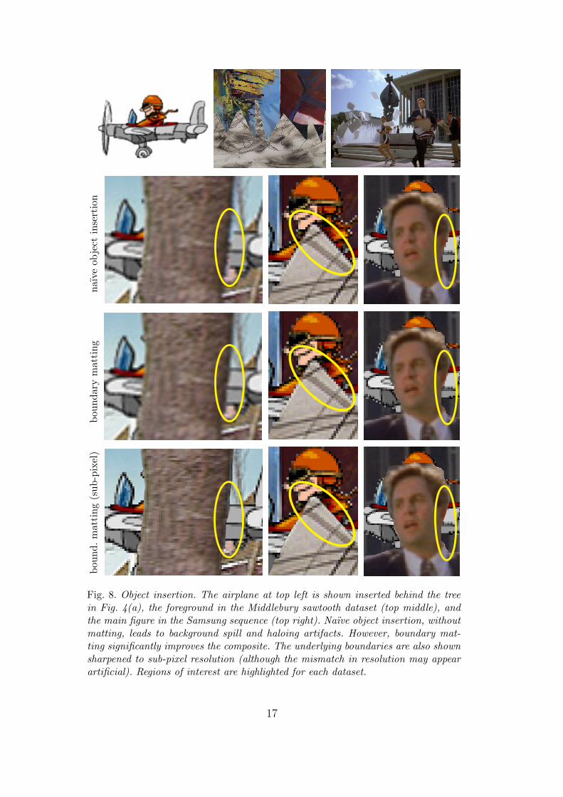
Next, we applied boundary matting to insert a new object between the fore-ground and background layers of three well-known stereo datasets (Fig. 8): theflower garden sequence (Fig. 4), the Middlebury sawtooth dataset [1] (Fig. 8,top middle), and the Samsung commercial sequence (Fig. 8, top right). Thesesequences are 344 × 240, 640 × 486, and 434 × 380 pixels respectively, withthe calibration accurate to within about 0.5 pixels. For the flower garden andsawtooth datasets, haloing artifacts from the background layer are clearly re-duced. Although the matting improvement is less dramatic for the Samsungsequence, this is mainly because the quality of naıve object insertion is rela-tively less objectionable, due to the high-quality initial stereo and the similar,desaturated colors of the foreground and background layers around the mainsubject’s head. The similarity of colors between foreground and backgroundlayers is also a source of ambiguity for the matting, particularly in the self-shadowed regions of the hair.

Not only does boundary matting improve the composites, but the extractedboundaries can even be sharpened by rendering the curves at sub-pixel resolu-tion (Fig. 8, bottom row). At close scales this sub-pixel rendering may appearless desirable for view synthesis due to the apparent resolution mismatch; how-ever the exact sub-pixel nature of the boundaries allows us to reblur them byany amount.

15

0 2.5 5 7.5 100

0.1

0.2

0.3

(%)noises

RM

SE

of

(on b

oundar

y)

a

ground truth noises = 0%

boundary matting

no matting

foreground

alpha m

attea

aF

noises = 5% noises = 10%

Fig. 7. Boundary matting synthetic data, with the addition of zero-mean Gaussiannoise. Top left: reference image of a planar textured ellipse, with zoomed region in-dicated. Top right: RMS error of α for pixels on the occlusion boundary. Bottom:visual comparison of the ground truth foreground and alpha matte with the bound-ary matting estimates given various levels of added noise. The naıve segmentationwithout matting is also shown for comparison.

Finally, the flower garden dataset was also used for a view synthesis task,for matting both an input view and a novel interpolated view (Fig. 9). Inboth cases, boundary matting produces a significant improvement over naıveview synthesis (i.e., forward warping with a fixed footprint, then featheringbetween the warped images). These results also demonstrate some tolerance toinaccurate stereo, since the initial stereo estimate in the region shown was upto two pixels off. We also experimented with a variety of settings for the blur

16

naı

ve

obje

ctin

sert

ion

bou

ndar

ym

atti

ng

bou

nd.m

atti

ng

(sub-p

ixel

)

Fig. 8. Object insertion. The airplane at top left is shown inserted behind the treein Fig. 4(a), the foreground in the Middlebury sawtooth dataset (top middle), andthe main figure in the Samsung sequence (top right). Naıve object insertion, withoutmatting, leads to background spill and haloing artifacts. However, boundary mat-ting significantly improves the composite. The underlying boundaries are also shownsharpened to sub-pixel resolution (although the mismatch in resolution may appearartificial). Regions of interest are highlighted for each dataset.

17

(a) (b) (c) (d) (e)

Fig. 9. Boundary matting for view synthesis. The first row corresponds to the refer-ence view, and the second row corresponds to an interpolated view. (a) Input image(ground truth interpolated view). (b) Zoomed-in region. (c) Naıve foreground sepa-ration without matting shows significant spill from the background layer. (d) Usingthe boundary matting method reduces this artifact. (e) Boundary matting with ablurred edge model (σ = 0.4 pixels) better matches the blur in the input images.

parameter. While the addition of blur did not appear to improve the mattingfor this case, the optimal blurred boundary better matches the appearance ofthe input images.

For this portion of the dataset, some degree of blue spill from the sky remainseven after performing boundary matting (Fig. 9(d–e)). This may be due to theoptimization being trapped in a local minimum because of poor initialization.Another explanation is that the object curves smoothly enough that it cannotbe accurately modeled using a single 3D boundary curve, and the boundaryshown truly represents the global best-fit approximation.

Our method broke down completely for the upper-left region of the tree con-taining many twigs (Fig. 10), yet still performs no worse than naıve view syn-thesis ignoring matting. The reason for failure was not an inability to localize aconsistent 3D curve, but rather that inaccurate stereo led to an initial bound-ary up to 30 pixels off. Without additional color-based priors, our mattingmethod is content to accept depth discontinuities across untextured regionsof sky, trapping the optimization in spurious local minima with F = B.

18

(a) (b)

Fig. 10. Boundary matting failure case. (a) Inaccurate stereo leads to a poor ini-tial boundary estimate in a mainly untextured region, which cannot be refined suc-cessfully by locally optimizing the matting. Very thin structures such as the smallbranches may also pose difficulties. (b) Object insertion highlights the severity of theproblem, although view synthesis is less objectionable in this region.

7 Concluding remarks

For seamless view interpolation, mixed boundary pixels must be resolved intoforeground and background components. Boundary matting appears to be auseful tool for addressing this problem in an automatic way. Using 3D curvesto model occlusion boundaries is a natural representation that provides severalbenefits, including the ability to super-resolve the depth maps near occlusionboundaries.

A current limitation of our approach is its lack of reasoning about color sta-tistics, which has proven very useful in natural image matting [9,2]. Such anability might enable us to resolve boundaries even in areas where stereo givesgrossly incorrect depths, as in the upper-left region of the tree in Fig. 4(a).By integrating boundary matting with complementary aspects of pixel-basedmatting methods [9,3], we hope to extend the generality of boundary mattingwhile retaining its superior view synthesis.

In the future, we would also like to adapt boundary matting to a dynamicstereo framework, where disocclusions over time may reveal additional infor-mation to improve the matting.

References

[1] D. Scharstein, R. Szeliski, A taxonomy and evaluation of dense two-frame, stereocorrespondence algorithms, Intl. Journal of Comp. Vision 47 (1) (2002) 7–42.

[2] Y.-Y. Chuang, A. Agarwala, B. Curless, D. H. Salesin, R. Szeliski, Videomatting of complex scenes, in: Proc. ACM SIGGRAPH, 2002, pp. 243–248.

19

[3] Y. Wexler, A. W. Fitzgibbon, A. Zisserman, Bayesian estimation of layers frommultiple images, in: Proc. ECCV, Vol. 3, 2002, pp. 487–501.

[4] H.-Y. Shum, J. Sun, S. Yamazaki, Y. Li, C.-K. Tang, Pop-up light field:An interactive image-based modeling and rendering system, in: Proc. ACMSIGGRAPH, 2004, pp. 143–162.

[5] C. L. Zitnick, S. B. Kang, M. Uyttendaele, S. Winder, R. Szeliski, High-quality video view interpolation using a layered representation, in: Proc. ACMSIGGRAPH, 2004, pp. 600–608.

[6] R. Szeliski, P. Golland, Stereo matching with transparency and matting, in:Proc. ICCV, 1998, pp. 517–526.

[7] A. R. Smith, J. F. Blinn, Blue screen matting, in: Proc. ACM SIGGRAPH,1996, pp. 259–268.

[8] M. Ruzon, C. Tomasi, Alpha estimation in natural images, in: Proc. CVPR,2000, pp. 18–25.

[9] Y.-Y. Chuang, B. Curless, D. H. Salesin, R. Szeliski, A Bayesian approach todigital matting, in: Proc. CVPR, 2001, pp. 264–271.

[10] P. Hillman, J. Hannah, D. Renshaw, Alpha channel estimation in high resolutionimage and image sequences, in: Proc. CVPR, 2001, pp. 1063–1068.

[11] C. Rother, A. Blake, V. Kolmogorov, “GrabCut” – Interactive foregroundextraction using iterated graph cuts, in: Proc. ACM SIGGRAPH, 2004, pp.309–314.

[12] J. Sun, J. Jia, C.-K. Tang, H.-Y. Shum, Poisson matting, in: Proc. ACMSIGGRAPH, 2004, pp. 315–321.

[13] R. Szeliski, S. Avidan, P. Anandan, Layer extraction from multiple imagescontaining reflections and transparency, in: Proc. CVPR, 2000, pp. 246–253.

[14] Y. Tsin, S. Kang, R. Szeliski, Stereo matching with reflections and translucency,in: Proc. CVPR, 2003, pp. 702–709.

[15] M. Irani, B. Rousso, S. Peleg, Computing occluding and transparent motions.,Intl. Journal of Comp. Vision 12 (1) (1994) 5–16.

[16] J. D. Bonet, P. Viola, Roxels: Responsibility weighted 3D volumereconstruction, in: Proc. ICCV, 1999, pp. 418–425.

[17] S. W. Hasinoff, K. N. Kutulakos, Photo-consistent 3D fire by flame-sheetdecomposition, in: Proc. ICCV, 2003, pp. 1184–1191.

[18] S. Ju, M. J. Black, A. D. Jepson, Skin and bones: Multi-layer, locally affine,optical flow and regularization with transparency, in: Proc. CVPR, 1996, pp.307–314.

[19] S. Birchfield, C. Tomasi, A pixel dissimilarity measure that is insensitive toimage sampling, IEEE Trans. PAMI 20 (4) (1998) 401–406.

20

[20] T. Mitsunaga, T. Yokoyama, T. Totsuka, Autokey: Human assisted keyextraction, in: Proc. ACM SIGGRAPH, 1995, pp. 265–272.

[21] E. N. Mortensen, W. A. Barrett, Toboggan-based intelligent scissors with a fourparameter edge model, in: Proc. CVPR, 1999, pp. 2452–2458.

[22] K. Bala, B. Walter, D. Greenberg, Combining edges and points for interactiveanti-aliased rendering, in: Proc. ACM SIGGRAPH, 2003, pp. 631–640.

[23] A. W. Fitzgibbon, Y. Wexler, A. Zisserman, Image-based rendering using image-based priors, in: Proc. ICCV, 2003, pp. 1176–1183.

[24] A. Criminisi, A. Blake, The SPS algorithm: Patching figural continuity andtransparency by split-patch search, in: Proc. CVPR (1), 2004, pp. 342–349.

[25] T. Porter, T. Duff, Compositing digital images, in: Proc. ACM SIGGRAPH,1984, pp. 253–259.

[26] J. J. Koenderink, What does the occluding contour tell us about solid shape?,Perception 13 (1984) 321–330.

[27] S. B. Kang, R. Szeliski, J. Chai, Handling occlusions in dense multi-view stereo,in: Proc. CVPR, 2001, pp. 103–110.

[28] D. B. West, Introduction to Graph Theory, 2nd Edition, Prentice-Hall Inc.,2001.

[29] A. Hoover, G. Jean-Baptiste, X. Jiang, P. J. Flynn, H. Bunke, D. B. Goldgof,K. K. Bowyer, D. W. Eggert, A. W. Fitzgibbon, R. B. Fisher, An experimentalcomparison of range image segmentation algorithms, IEEE Trans. PAMI 18 (7)(1996) 673–689.

[30] J. Nocedal, S. J. Wright, Numerical Optimization, Springer, 1999.

[31] J. More, B. Garbow, K. Hillstrom, Minpack, http://www.netlib.org/minpack.

[32] M. Kass, A. Witkin, D. Terzopoulos, Snakes: Active contour models, Intl.Journal of Comp. Vision 1 (4) (1988) 321–331.

21