BOUNDARY LAYER TRANSITION IN SIMULATED

TURBINE BLADE FLOW

by

Derek Graham BSc

Department of Mechanical and Industrial Engineering, Dundee Institute of Technology

Thesis submitted to the C.N.A.A. in partial fulfilment of the requirements of the degree of Doctor of Philosophy

August 1990

DECLARATION

I hereby declare that the following work

has been composed by myself and that

this thesis has not been presented for

any previous award of the C.N.A.A. or

any other university

Derek Graham

ii

CONTENTS

Abstract v

Publications vi

Acknowledgements vii

Notation viii

1 INTRODUCTION 11.1 Blade Design 3

1.2 The Boundary Layer 6

1.3 Transition Prediction 9

1.4 Experimental Measurement of Intermittentlyturbulent flows 14

2 EXPERIMENTAL FACILITIES 192.1 Wind Tunnel Facility 19

2.2 Turbulence Generating Grids 21

2.3 Freestream Pressure Distribution 21

2.4 Hot Wire Instrumentation 22

3 DATA ACQUISITION 283.1 Data Transfer 28

3.2 Data Acquisition Hardware 30

3.3 Data Acquisition Software 32

3.3.1 Programming the 18086 343.3.2 Data Acquisition Subroutine 373.3.3 Main Data Acquisition Program 41

3.4 Signal Conditioning 44

4 DATA REDUCTION 55

4.1 Reduction of the Raw Data 56

4.1.1 Mean Velocity 564.1.2 RMS Subroutine 574.1.3 Intermittency Measurement 60

iii

4.2 Reduction of Mean Velocity Profiles 66

4.2.1 Reduction of Laminar Mean Velocity Profiles 664.2.2 Reduction of Turbulent Mean Velocity Profiles 684.2.3 Transitional Mean velocity Profiles 714.2.4 Start and End of Transition 73

5 DISCUSSION OF EXPERIMENTAL RESULTS 925.1 Start of Transition 94

5.2 Statistical Similarity of Transition Regions 97

5.3 Transition Length 99

5.3.1 N in Zero Pressure Gradient Flows 1025.3.2 N in Adverse Pressure Gradient Flows 103

5.4 Details of Transition 106

5.4.1 Integral Parameters 1065.4.2 Velocity Profiles 1085.4.3 Flow 7 110

6 BOUNDARY LAYER PREDICTION 1346.1 The Cebeci-Smith Method 134

6.2 Performance of the C-S Method 138

Conclusions 155

Suggestions for Future Work 159

References 161

Appendix 1 - Computer Program Listings 167

Appendix 2 - Experimental Data (Integral Parameters) 216

Appendix 3 - Experimental Data (Velocity Profiles) 225

Appendix 4 - Journal Publication, Fraser et al (1990) 257

iv

Boundary Layer Transition in Simulated Turbine Blade Flow

by

Derek Graham

Abstract

An experimental investigation of the development of the boundary layer in a simulated turbine blade flow is described.

A velocity distribution typical of a "squared-off" turbine blade was reproduced in an open return wind tunnel. Measurements were made in the boundary layer formed on a flat, polished aluminium plate using standard hot wire instrumentation. An automatic data acquisition and control system was based around an Amstrad PC1640 16-bit microcomputer. By using assembly language subroutines, very fast sampling rates could be achieved which allowed a detailed digital representation of the raw signal to be captured. The relatively large RAM capacity of the Amstrad PC1640 allowed samples of sufficient duration to be stored. The mean flow variables, such as the mean velocity and RMS, were calculated by software thus reducing the requirement for external instrumentation. Assembly language subroutines were again necessary to process the large quantities of data involved within acceptable timescales.

An algorithm was developed to discriminate between laminar and turbulent flow. This was used to conditionally sample the signal in the transition region and hence provide mean laminar and turbulent velocity profiles in the transition region. It also provided a measurement of the intermittency. Boundary layer profiles were measured under the imposed velocity distribution at various levels of freestream turbulence giving a range of normal and separation bubble type transitions. The concept of statistical similarity of transition regions was observed to remain intact for severe adverse pressure gradients, including cases where separation bubbles were present during the early stages of transition.

An original correlation for the spot formation rate parameter, N, was developed using the adverse pressure gradient data of Gostelow (1989b). This correlation accounted for the combined effects of freestream turbulence and adverse pressure gradient. The correlation was found to give better prediction of the transition length in turbine blade flows than currently used methods.

The conditionally sampled velocity profiles indicate that intermittent laminar separation can occur in the early part of the transition region.

v

PUBLICATIONS

Fraser C J , Milne J S & Graham D

- "Fast Data Acquisition and Digital Signal Processing in Studies of Turbulent Flow" 4th Joint International Conference on Mechanical Engineering and Technology, Zagazig Univ. Cairo, 1989Paper presented by Dr C J Fraser

Graham D, Fraser C J & Milne J S

- "Digital Measurement inIntermittently Turbulent Flows" AMSE conference on Signals and Systems, Brighton, 1989 Paper presented by D Graham

Fraser C J , Graham D & Milne J S

- "Digital Processing of Hot Wire Anemometer Signals in Intermittently Turbulent Flows" Flow Measurement and Instrumentation, Vol. 1, 1990

vi

ACKNOWLEDGEMENTS

I would like to sincerely thank the following people;

My supervisors, Dr C J Fraser and Mr J S Milne, who at all times have shown a keen interest in the development of the project.

Dr P Stow and Mr N T Birch of Rolls-Royce PLC who provided much information and valuable comment during the course of the project.

The technical staff, in particular Mr W Keating for assistance in the laboratory and Mr I McNab and Mr R Greig. Also Noreen and Liz of the secretarial staff.

Finally a special thanks to my collegues Sumant Mathure and George Kotsikos.

The financial support of Rolls Royce PLC and the SERC is gratefully acknowledged.

vii

NOTATION

A dependence areaa velocity ratio of upstream edge of a

spotturbulent

b velocity ratio of downstream edge of turbulent spot

a

C constant in the law of the wallc£ skin friction coefficientc wave propagation speedf dimensionless stream function

G spot formation rate parameter

g spot production rate (from Emmons (1951))or H S* / e shape factor

i T7!L mixing lengthm i l du

v dxpressure gradient parameter

m x dU U dx

pressure gradient parameter (chapter 6 )

n spot formation rate (no./s m)n number of points (section 4.1.3)N non-dimensional spot formation rateR influence volume

Roc. xUV

length Reynolds number

Re 0UV

momentum thickness Reynolds number

Rx AUu

transition length Reynolds number

r body radiuss streamwise surface distance

viii

Tu% freestream turbulence levelt timeAt small, finite time intervalu, v, w instantaneous velocity components (m/s)u',v', w' fluctuating velocity components (m/s)U, V, w mean velocity components (m/s)

u t Vt'w/P friction velocity (m/s)+u u / u ^ dimensionless velocity

U freestream velocity (m/s)V volume in xyt spacex, y, z cartesian coordinates (mm)X location of 50% intermittency point (mm)Ax transition length as defined by Chen and Thyson

(1971)

y + y^x/v dimensionless y coordinatea anglea wave number

P non dimensional coordinate (equation 4.19)stream function

€ eddy viscosityA distance between 25% and 75%

intermittency points (mm)

V X - X o

transition normalising coordinate (Schubauer and Klebanoff (1955))

K constant in the law of the wallCO vorticity

V fluid dynamic viscosity (kg/ms)V fluid kinematic viscosity (m2 /s)

p fluid density (kg/m3)n Coles' wake parameter

ix

7 near wall intermittency

e momentum thickness (mm)a dependence area factor

a standard deviation of mean intermittency distribution (mm)

T shear stress

i X - X+.A

transition normalising coordinate (Dhawan and Narasimha (1958))

6 boundary layer thickness (mm)4?8 displacement thickness (mm)

subscriptsL laminar flowd downstream edge of turbulent spoti inner region (chapter 6 )o outer region (chapter 6 )o zero pressure gradient flowss start of transition (1 % intermittency point)t start of transition (Narasimha's criterion)tr related to the transition regionT turbulent flow

u upstream edge of turbulent spotw conditions at the wall

xO

CHAPTER 1

INTRODUCTION

The first gas turbine design was patented in 1791 by John Barber but it was not until the early years of the twentieth century that the first successful turbines were built. In Britain nearly 2 0 0 patents for gas and steam turbines were registered between 1784 and 1884, the year in which Parsons successfully constructed a steam turbine. The implications of Parsons invention became clear in 1897 when his turbine propelled boat, the Turbinia proved to be faster than the Royal Navy's fastest destroyers of the time. The 1930s proved to be a productive period in the development of the gas turbine. In 1939 the first jet powered flight was made in Germany and the Brown Boveri company demonstrated the first gas turbine power plant at the Swiss National Exhibition in Zurich. Gas and steam turbines are now used in many applications and have become increasingly more efficient as improvements in materials, cooling techniques and subsequent operating temperatures have been achieved. However, in recent years factors such as increased competition, government regulations on noise and emissions and dramatic changes in prices and availability of fuel have ensured continuing efforts to further improve the performance and efficiency of gas and steam turbine engines. Although the present work is specific to gas turbines it does have some relevance to non condensing steam turbines.

In the past intuitive design played a considerable role with the design and construction of working engines often preceding a theoretical understanding of all the processes involved. Even now the ideal of purely theoretical prediction of the performance of an arbitrary blade cascade is far in the future. The flow fields associated with turbomachinery are extremely complex. They are

1

three dimensional, unsteady, highly turbulent and subject to strong rotational effects. Theoretical analysis can be further complicated by other factors such as supersonic effects and the need to apply external and internal cooling to turbine blading. These effects are illustrated in figures 1.1a and 1.1b

According to Dzung and Seippel (1970) one of the first attempts to calculate the flow field around a blade was made in 1906 by Lorentz, who made the unjustified assumption that all streamlines were congruent to the blade shape. The 1920s saw the advent of the aircraft industry and the accumulation of aerofoil data which prompted the application of aerofoil theory to the prediction of turbine blade performance. The theory of two dimensional, inviscid flow was already well developed and methods of solving the Laplace equation, for example conformal mapping, were well known and could be applied to simple blade shapes. Arbitrary blade shapes, however, only became more readily analysed after the introduction of digital computers. Schlichting and Scholz were the first to account for the effect of viscosity by utilising Prandtl's boundary layer concept in 1951, almost fifty years after it was introduced.

Accurate flow prediction methods can play an important part in the design of turbine blading. In particular, prediction of the development of the boundary layer over blade profiles is important since it directly represents the aerodynamic losses and heat transfer associated with the blade. Current boundary layer prediction methods, however, are unreliable in important areas such as laminar to turbulent transition. Faster, more reliable, prediction methods, which can be used to analyse on-design and

2

off-design conditions, will allow more detailed optimisation without increasing development costs and should lead to better final designs.

1.1 BLADE DESIGN

Computer aided blade design systems typically consist of two parts, a through-flow analysis and a blade to blade analysis. The through-flow analysis gives information about the inlet and outlet flow conditions which are necessary to determine parameters such as stage pressure ratio or work output and the blade to blade analysis is used to determine the flow behaviour between individual blades.

The through-flow calculation considers the flow through a number of stages. Small scale unsteadiness in the flow, such as blade wakes, are ignored and the three dimensional equations of motion are usually reduced to a two dimensional form. The equations of motion are further modified to allow the effects of the blades on the through-flow to be modelled. For example, a dissipative force is included to account for the viscous losses through a blade row. Other effects which are modelled include; end wall boundary layers, secondary flows, various leakage flows etc. A more detailed description of through-flow modelling is given by Stow (1989).

The detailed flow over individual blades is normally calculated by coupling inviscid and boundary layer calculations, however methods which solve the Navier-Stokes equations have emerged in recent years. Solution of the complete Navier-Stokes equations requires considerable computing time with the fastest computers and is impractical for most cases. For turbulent flows

3

the time averaged, or Reynolds averaged, form of the Navier-Stokes equations are often used in conjunction with a model for the turbulence. Two approaches to inviscid analysis are possible; the design approach where the desired velocity over the blade is prescribed and the analysis gives the necessary blade geometry, and the analysis approach where the blade geometry is prescribed and the external velocity is calculated. Both approaches are useful and methods have been developed which combine both, for example the method of Cedar and Stow (1985) which is based on the finite element technique.

The boundary layer equations are a simplification of the Navier-Stokes equations and are valid in the region close to the surface of a body when the Reynolds number, based on the length of the body, is greater than about 1000. However the boundary layer equations are still complex, non-linear partial differential equations which are not readily solved for general boundary conditions. Various analytic approaches have been developed for laminar boundary layers. For example similarity solutions which reduce the number of variables, by one or more, by means of a coordinate transform. More general boundary layer calculation methods are based on either the von Karman integral momentum equation or direct numerical solution of the boundary layer equations using the finite difference technique. Integral methods are fast and acceptably accurate in many cases. Finite difference techniques require longer solution times and also rely on experimental data at some stage in the development of accurate turbulence models. For transitional flows integral methods and most finite difference methods require correlations to determine

4

the start and end of transition.Inviscid - boundary layer coupling involves using the

solution from a boundary layer calculation to modify the inviscid mainstream calculation. This is done by thickening the blade by the boundary layer displacement thickness before recalculating the inviscid flow over the modified blade shape. The boundary layer calculation is then repeated to give a new modified blade shape and this procedure is repeated until subsequent boundary layer calculations converge within specified limits.

At off design conditions laminar separation bubbles, where the flow reattaches as a turbulent boundary layer, can occur near the leading edge, Also, in some cases, complete turbulent separation can occur towards the trailing edge. Under these conditions the coupled inviscid - boundary layer approach can become very unreliable as the boundary layer approximations become invalid. Because of the importance of being able to predict off design losses, methods of solving the Reynolds averaged Navier-Stokes equations in two dimensions are currently being developed and used. These methods still rely on relatively simple turbulence models and the start and end of transition is specified or determined by correlation. Birch however (1987a) uses a one equation kinetic energy model for turbulence and transition. Although these methods have proved better able to predict off design flow conditions they will not replace the inviscid - boundary layer methods as every day design tools unless they become faster and cheaper to run. Three dimensional Navier-Stokes methods have also been developed and are used to some extent in design applications at present.

5

1.2 THE BOUNDARY LAYERThe introduction of the boundary layer concept by Prandtl in

1904 has proved to be one of the most significant achievements in the development of viscous flow theory and its importance in turbomachinery design has already been stated. The boundary layer concept allowed the theory of ideal fluid flow, which had been developed in the eighteenth century by such as Bernoulli, Euler, Lagrange and Laplace, to be reconciled with observations of the real world and the viscous -inviscid matching procedure permitted meaningful analysis of viscous flows.

The behaviour of the boundary layer is rather complex. Near the leading edge, in two dimensional flow, the flow is always laminar but at some point downstream it becomes unstable. Stability theory for viscous flow originated with the work of Orr (1907) and Sommerfeld (1908) who independently derived what is now known as the Orr-Sommerfeld equation ie.

(u - c) (v' ' - a2v) - u''v + i^(v' ' ' ' - 2 a 2v' ' + a 4v) = 0 (1 .1 )a

where a = disturbance wave number, c = wave propagation speed, i = J - 1 , v = the disturbance variable and the prime, ', denotes differentiation w.r.t. y.

Solution of this equation can reveal whether infinitesimal disturbances are damped (stable flow) or amplified. The Reynolds number at which laminar flow becomes unstable to a travelling wave disturbance was calculated by Tollmein (1929) and extended to amplified two dimensional disturbances by Schlichting in the 1930s. These disturbances, which are now called Tollmein-Schlichting waves, were not observed experimentally until 1940-1941 by

6

Schubauer and Skramstad (1948). Previous to this the existence ofTollmein-Schlichting waves had not been accepted outwith Germany partly because of the political situation prior to the second world war and partly because of the lack of experimental evidence. As the flow develops, the Tollmein-Schlichting waves are amplified and soon become three dimensional. Ultimately, isolated spots of turbulence emerge which grow as they travel downstream and merge to form a fully turbulent boundary layer. The transition region consists of spots of turbulence surrounded by essentially laminar flow and is quantified by the intermittency function, 7 , which defines the probability of encountering turbulence at any point and varies from 0 in laminar flow to 1 in the fully turbulent boundary layer.

Schubauer and Klebanoff (1955) provided the first quantitative data on the shape, growth and propagation of turbulent spots. Various workers including Chen and Thyson (1971), McCormick (1968) and more recently Walker (1987) have subsequently approximated the turbulent spot as a two dimensional triangle with the vertex downstream. Since then various workers have made more detailed studies of the structure and behaviour of turbulent spots. Wygnanski et al (1976) have measured the three dimensional

mean flow field within a spot using ensemble averaging techniques. Cantwell et al (1978) studied the structure and growth in the plane of symmetry of a spot and Gad-el-Hak et al (1981) further investigated the growth of spots both normal to the plate and in the spanwise direction. All the above work was carried out in zero pressure gradient flows.

The first integral method, which was appropriate only for

7

laminar boundary layers, was devised by Pohlhausen (1921) and was based on the integral momentum equation of von Karman. Pohlhausen's method was widely used for about twenty years before better methods were developed. Twenty integral methods for turbulent boundary layers are described in the proceedings of the Stanford conference, see Kline et al (1968), and four of those were graded good when tested against a variety of data. Dhawan and Narasimha (1958) showed that the transitional boundary layer could be adequately described by performing laminar and turbulent calculations and weighting the solutions using the intermittency. This represented a considerable improvement over the assumption of point transition, particularly when the transition region occupied a considerable proportion of the flow. The finite difference technique is an old one but has only been a practical tool for solving the boundary layer equations since the introduction of the digital computer. The laminar boundary layer equations can be solved with arbitrary accuracy but turbulent boundary layer calculations depend on the accuracy of the turbulence model used. The most popular approach is to use an eddy-viscosity model as used by two of the three methods which were graded "good" at the Stanford conference. Various methods have been used to predict transition, for example McDonald and Fish (1973) use the turbulent kinetic energy transport equation, but it is still common to find empirical and semi empirical correlations for the start and length of transition, eg. Cebeci and Smith (1974).

The assumptions which allow the Navier-Stokes equations to be reduced to the boundary layer equations do not apply close to the point of separation, in particular velocities in the y direction

8

become significant. As a result both integral and differential methods have difficulty in predicting flows with severe adverse pressure gradients where separation is present. Integral methods resort to empirical correlations, such as Horton (1967), for laminar separation and reattachment. The so called FLARE

approximation used by Cebeci, Keller and Williams (1979) allows the method of Cebeci and Smith (1974) to continue through small regions of separated flow but requires that the displacement thickness be specified.

1.3 TRANSITION PREDICTIONIntegral and differential methods can give good predictions

of the behaviour of the important parameters through transition but only if the start and end of transition are known. However, the inability to predict the start and length of the transition region is perhaps the most severe limitation to accurate prediction of typical blade boundary layers, Birch (1987b). The theory of linear stability can predict the point where laminar flow becomes unstable but it becomes increasingly more difficult to continue when three dimensionality becomes important. The boundary layer remains essentially laminar until the first turbulent spots form in the flow marking the start of transition. Various semi-empirical approaches to the prediction of transition onset, such as the so called en methods which relate the location of the start of transition to the amplification of Tollmein-Schlichting waves, have been proposed. However in some applications, such as turbine blade flows, it is still more common to find empirical correlations being used. A very commonly applied correlation is that of Abu-Ghannam

9

and Shaw (1980) which is the most recent and is based on the mostdata.

Dhawan and Narasimha (1958) proposed a correlation for transition length which related the transition length Reynolds number to the Reynolds number based on the location of the start of transition. Good correlation has been observed for zero pressuregradient flows with much of the scatter attributable to thediffering techniques used to detect the start and end oftransition. However, direct application of the Dhawan andNarasimha correlation to flows with pressure gradients can give poor accuracy. The transition length prediction method of Chen and Thyson (1971) is based on a similar correlation but also allows local conditions to affect the growth of turbulent spots and thus affect the calculated length of transition. A correlation for transition length which takes into account the effects of freestream turbulence and pressure gradient was proposed by Fraser et al (1988), for adverse pressure gradients only.

Emmons (1951) made the first attempt to quantify the transition process by means of a probability analysis. He assumed the existence of a function, g(x,y,t), of position on the surface and time which specified the rate of spot production per unit area and followed the subsequent development of each spot produced. The fraction of time, 7 (x,y), (Emmons used the notation f(x,y)) that a point P(x,y) is turbulent is obtained by summing the times that it is covered by a spot, taking care not to count overlapping spots twice. A spot generated at P0 (x0 , yQ , t ) sweeps out a volume in xyt space which Emmons called the "propagation cone". He also noted that the cone need not have straight generators, allowing for

10

non linear growth of the spot as in axi-symmetric flows, for example. Emmons also defined the "dependence cone" which, for P(x,y,t), is the locus in xyt space of all points P0 (x0 ,y0 ,t0) such that spots generated at these points will cover P. To eliminate errors due to overlaps Emmons assumed that the spot formed closest to the leading edge would be taken as causing the turbulence. Thus he developed an expression for the fraction of time, 7 (P), during which the flow at P is turbulent ie.

7(P) “ 1 - exp(-/R g(P0 )dV0 ) (1.2) which can be calculated numerically if g(P0 ) is known and the influence volume R is defined. Emmons considered flat plate flow and assumed that g was constant. He also assumed that both the propagation and dependence cones had straight generators and thus the volume, V, of the dependence cone was given by V = A 1x3/3 where Aj is the cone cross section at unit distance from the apex. Thus Emmons derived the intermittency distribution

7 (x) = 1 - exp(-ogx3 /3U) (1.3) where cr is a dimensionless propagation parameter of the spot related to the base area of the cone at unit distance from the apex.

The spot concept of transition was investigated by the experiments of Schubauer and Klebanoff (1955), however their intermittency measurements did not agree with Emmons' theory. Instead they fitted their data to a cumulative normal distribution and showed that, when scaled by the standard deviation, all the data collapsed onto a single curve. Dhawan and Narasimha (1958) managed to reconcile Emmons' theory with experimental data by introducing the concept of concentrated breakdown. This stated

11

that turbulent spots were most likely to appear at a fixed point in the flow and this point was observed experimentally to be the start of transition. They assumed g to be a Gaussian error curve with its maximum at xt and found the best agreement with experimental data when the Gaussian curve had a standard deviation approaching zero. Thus they assumed g to be best approximated by a Dirac delta function. Using Emmons' theory this gave the intermittency distribution

7 = 1 - exp[-(x - xt)2na/U] (1.4) where n is the number of spots occurring per unit of time and spanwise distance at xt. This can be modified to give the '’universal" distribution

7 = 1 - exp(-0.412£2) (1.5) where £ = (x - xt)/A with A being the distance between the points where the intermittency is 0.25 and 0.75. Dhawan and Narasimha showed that intermittency data for a flat plate collapsed onto this single curve, when normalised by A, whether transition was natural or provoked by a trip wire. The concept of statistical similarity of transition regions has been extended to moderate adverse pressure gradients by Fraser et al (1988), Gostelow and Blunden(1988) and Gostelow (1989) and was shown to remain intact, in fact the present work has indicated that it holds true in severe adverse pressure gradients.

From the above two equations it can be shown thatn = 0.412U/aA2 (1.6)

ie. that the transition length varies as the inverse square root of the spot formation rate, if a is constant. Emmons estimated the value of a as about 0.1 and Narasimha (1985) found that a varies

12

from about 0.25 to 0.29. Knowledge of the behaviour of a is limited since detailed measurements of spot shapes only exist for zero pressure gradient flows. Narasimha (1985) defined the non dimensional parameter

N = na6*/v (1.7)and suggested that it has a constant value of 0.7 x 10“ 3 in zero pressure gradient flows. Data indicates that this value increases at low freestream turbulence levels. The work of Gostelow and Blunden (1988), Gostelow (1989a), Walker and Gostelow (1989) and the present work have shown that N rises rapidly in adverse pressure gradients and also varies greatly with freestream turbulence. In the course of the present work the data set of Gostelow (1989b) has been used to correlate N with the pressure gradient and freestream turbulence level.

Chen and Thyson (1971) extended Emmons theory to include blunt, axisymmetric bodies with pressure gradients. They accepted the hypothesis of concentrated breakdown and assumed that a) spot propagation velocities were proportional to the local external velocity and b) the spot grows at a constant angle, a, relative to the local external streamline. Thus they developed the following

expression for intermittency7 = 1 - exp[ -Gr(st)( f r~1ds)( f Ue~1 ds)] (1.8)

where G is a new spot formation rate parameterG = ntana(a" 1 - b"1), with a = Uu/Ue and b = Ud/Ue

G was then correlated with the start of transition Reynolds number, Re , and Mach number for a flat plate. The method is still widely used but has been found to predict transition lengths which are far too long in adverse pressure gradients. The fact that the method

13

is not solely dependent on the conditions at the start of transition has lead to suggestions that it may be better able to predict transitions which occur in flows with rapidly varying pressure gradients, for example a flow where transition starts in a favourable pressure gradient and continues into a region of adverse pressure gradient, although this has been disputed by Narasimha (1985).

The fact that the intermittency distribution remains statistically similar in favourable and adverse pressure gradients might be taken to indicate that effects on the spot growth and propagation characteristics may have a secondary influence on the transition length. In fact Narasimha (1985) quotes one case where a pressure gradient occuring in the downstream half of the transition region has no effect on the intermittency distribution. This suggests that the most important factor influencing the extent of the transition region is the rate at which spots are produced at the start of transition, which can be quantified by the parameter N. This also gives some physical justification to the correlations which relate the length of transition to conditions at the start of transition although more sophisticated correlations may be necessary to account for pressure gradient and other effects. It is this physical justification which makes the spot formation rate approach to transition length prediction more attractive than purely empirical correlation.

1.4 EXPERIMENTAL MEASUREMENT OF INTERMITTENT FLOWSSchubauer and Klebanoff (1955) obtained measurements of

intermittency in the transition region directly from photographic

14

records of an oscilloscope trace. At around the same time Corrsin and Kistler (1955) were using conditional sampling to investigate the intermittent turbulence which occurs in the outer region of the turbulent boundary layer. This area was further studied by Kovasznay et al (1970) who developed new techniques of conditional sampling and conditional averaging using analogue equipment, and also by Kaplan and Laufer (1962) and, more recently, by Murlis et al (1982) using large digital computers. Arnal et al (1977)

applied conditional sampling to the transition region on a flat plate and showed that the behaviour of turbulent spots was very similar to that of a fully developed turbulent boundary layer from an early stage, giving credence to the assumption adopted by Dhawan and Narasimha (1958) . The signal from a hot wire anemometer was first recorded in analogue form and then digitised at an effective sampling rate of 10kHz before processing in a digital computer.

During the course of the present work a data acquisition and control system, based on the IBM compatible AMSTRAD PC1640, was developed. £ real time sampling rate of 10kHz was employed and sufficient memory space was available to allow long sample times to be obtained. The use of the 16-bit microcomputer has allowed the development of a powerful digital system which would previously have required access to an expensive mainframe or mini computer.

Using a conditional sampling technique the system was used to investigate the transitional boundary layer on a simulation of the suction surface of a turbine blade. One feature of particular interest was the possibility of intermittent separation occurring in a transitional boundary layer where the turbulent component of

the flow remains attached as suggested by Gardiner (1987). The

15

development of the data acquisition system has resulted in the presentation of two conference papers; Fraser et al (1989) and Graham et al (1989), and one journal publication; Fraser et al (1990) (see appendix 4).

16

Laminar H Rotation

Figure 1.1a: 2D Turbine Blade Flow

Figure 1.1b: 3D Turbine Blade Flow17

CHAPTER 2

EXPERIMENTAL FACILITIES

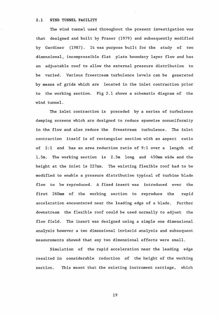
2.1 WIND TUNNEL FACILITYThe wind tunnel used throughout the present investigation was

that designed and built by Fraser (1979) and subsequently modified by Gardiner (1987). It was purpose built for the study of two dimensional, incompressible flat plate boundary layer flow and has an adjustable roof to allow the external pressure distribution to be varied. Various freestream turbulence levels can be generated by means of grids which are located in the inlet contraction prior to the working section. Fig 2.1 shows a schematic diagram of the wind tunnel.

The inlet contraction is preceded by a series of turbulence damping screens which are designed to reduce spanwise nonuniformity in the flow and also reduce the freestream turbulence. The inlet contraction itself is of rectangular section with an aspect ratio of 2 : 1 and has an area reduction ratio of 9:1 over a length of 1.5m. The working section is 2.5m long and 450mm wide and the height at the inlet is 227mm. The existing flexible roof had to be modified to enable a pressure distribution typical of turbine blade flow to be reproduced. A fixed insert was introduced over the

first 260mm of the working section to reproduce the rapid acceleration encountered near the leading edge of a blade. Further downstream the flexible roof could be used normally to adjust the flow field. The insert was designed using a simple one dimensional analysis however a two dimensional inviscid analysis and subsequent measurements showed that any two dimensional effects were small.

Simulation of the rapid acceleration near the leading edge resulted in considerable reduction of the height of the working section. This meant that the existing instrument carriage, which

19

ran inside the working section on two horizontal rails fixed to the side walls, would produce an unacceptably large blockage to the flow. The solution adopted was to move the carriage outside the working section and provide access for the hot wire probe by means of a slot in the roof. The slot was then sealed using an adhesive tape. This arrangement, however, limited all measurements to the centre line of the working section. Streamwise positioning of the probe was carried out manually and vertical traversing was driven remotely by means of a DISA sweep drive unit (type 52B01) in conjunction with a stepper motor (type 52C01). A pitot static tube coupled to an inclined manometer, which was used to calibrate the probe and monitor the reference velocity had to be moved from the leading edge to a point 780mm downstream.

A flexible coupling connects the exit of the working section to the diffuser. This prevents vibrations being transmitted from the fan and the motor to the working section and also provides a pliable seal between the variable height roof and the diffuser. The diffuser merges from a 450mm by 450mm square section at the upstream end to an 800mm diameter round section over its 1.5m length. The six blade fan is driven by a 2hp variable speed motor which has a maximum speed of 1440rpm and is housed in a 700mm long cylindrical casing.

The wind tunnel is equipped with an aluminium boundary layer plate which is 6mm thick, 2.4m long and spans the full width of the working section. The plate was originally positioned 50mm above the floor of the working section at zero incidence to oncoming flow. The symmetrically sharpened leading edge was bent downwards

to ensure that the stagnation point would occur on the upper

20

surface of the leading edge. Gardiner (1987) modified the leading edge design, returning it to a symmetrical shape and ensured that the stagnation point would occur on the top surface by inclining the plate at -0.5 degrees to the oncoming flow.

2.2 TURBULENCE GENERATING GRIDSVarious levels of freestream turbulence were generated in the

working section by inserting grids close to the contraction entrance, about 400mm downstream of the front edge. This arrangement was suggested by Blair et al (1981) and differs from the arrangement employed by most other wind tunnels in which the grids are located at the start of the working section itself, eg. Roach (1988) . The advantage of this arrangement is that the turbulence generated will be more homogeneous and have a lower decay rate along the test section although a coarser grid will be required for a given turbulence intensity. Four existing grids were used to produce turbulence levels at the leading edge of between 1% and 1.5%. A further grid was designed to give a leading edge turbulence level of about 2 %.

2.3 FREESTREAM PRESSURE DISTRIBUTIONThe wind tunnel was arranged to reproduce the velocity

distribution found on the suction surface of a forward loaded aerofoil ("squared-off" design). The velocity distribution was based on that used by Sharma et al (1982) which is described in detail by Gardner (1981) and is shown in fig 2.2. The rapid acceleration which occurs over the first 10-15% of the blade could not be achieved simply by means of the existing flexible roof so a

21

section was designed which would be fixed in place over the leading edge region. The shape of the insert was calculated using the one dimensional continuity equation. A two dimensional, inviscid calculation was carried out using a finite element package, the results of which indicated that variation of the velocity in the y direction would be small and would thus not affect the development of the boundary layer. This was confirmed experimentally after the

roof insert was installed. Measurements also showed that the roof boundary layer was turbulent from the earliest measuring station and there appeared to be no separation from the roof which could have caused problems in setting up the required velocity distribution.

Figure 2.3 shows the variation of the freestream turbulence intensity and the RMS of u' along the test section, with the highest turbulence generating grid present. The turbulence intensity appears to vary in inverse proportion to the freestream velocity. The RMS of the fluctuations in u do not appear to be strongly influenced by the rapid acceleration and deceleration of the flow, varying by less than 10% over the first 700mm of the test section.

2.4 HOT WIRE INSTRUMENTATIONAll velocity measurements were made using standard DISA,

series 55M hot wire instrumentation. Boundary layer probes were connected via a probe support and a 5m length of coaxial cable to a 55M10 constant temperature anemometer. The voltage output from the anemometer is related to the velocity over the probe but the relationship is non-linear. The signal is passed through a 55M25

22

lineariser which can be calibrated to give an output which is linearly proportional to the flow velocity. The output from the lineariser is passed through a 55D25 auxiliary unit to filter out frequencies above 2kHz since most of the turbulent energy is contained well below this frequency.

23

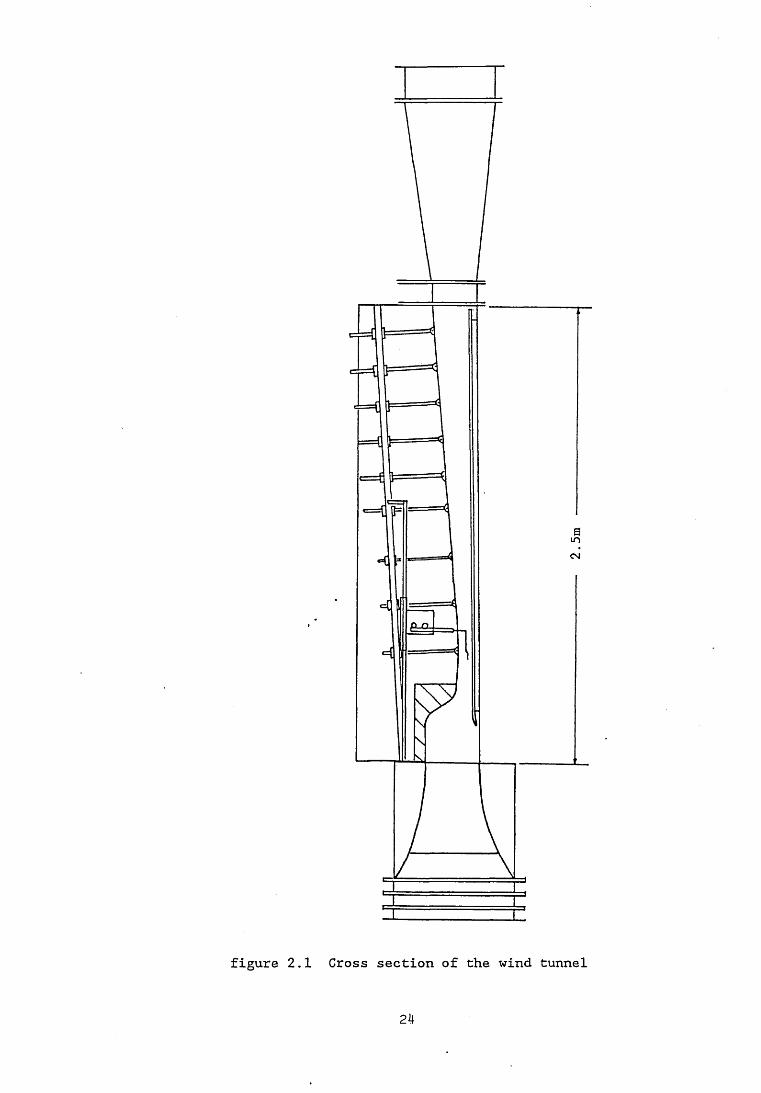
figure 2.1 Cross section of the wind tunnel

2 4

velocity distribution of Sharma et al (1982)

U m/s 1 aI W

14 H

12 H

10 i

z.,/n

i0 200 400 600 800 1000

x (mm)

Sharma et al D present data

figure 2.2

25

freestream turbulence distribution

Ti2.5 i

[D2 1

1.5 i

1 -t

0.5 J

0 T

0

!% vAF- 0.25

n Tu% A RMS u’

figure 2.3 distribution of freestream turbulence and RMS of u’

0.2

A

u

A A A

n□ D

n □

0.15

n^ 0.1

L 0.05

200 400 x (mm)

or> uu vJ 800

26

CHAPTER 3

DATA ACQUISITION

Since the introduction of the first commercial microprocessor chip by Intel, the 4-bit Intel 4004 in 1971, the microcomputer has found increasing application to engineering problems. 8-bit machines, such as the BBC microcomputer, have proved very successful in measurement and control systems but it is only with the advent of 16-bit machines, such as the IBM and compatible machines, that the microcomputer has begun to pose a threat to mainframe computers in some applications.

Traditionally the measurement of turbulent flows has involved the use of expensive analogue instrumentation but a digital computer based approach can be much more flexible. Previously this required access to a mainframe or mini computer but the increased memory capacity of the 16-bit computers allows these machines to be used in data acquisition applications although there may be a time penalty when analysing large quantities of numerical data. This chapter describes the development of a data acquisition and control system, based on an IBM compatible 16-bit machine, which allows detailed digital measurements to be made in transitional boundary layers. The sophistication of the system is comparable to that achieved in the past by workers using mainframe computers but at a

fraction of the cost.

3.1 DATA TRANSFERAn important consideration in the development of a computer

based data acquisition system is the process by which data is to be transferred between the external instrumentation and the computer itself. One approach is to use a standard digital transmission bus

such as the IEEE-488 parallel bus or the RS232 serial bus. Many

28

microcomputers have serial and parallel input/output ports and can communicate data directly in digital format with a wide range of compatible laboratory instruments. However, many instruments produce analogue signals, normally in the form of a voltage, to represent the physical quantity being measured or require an analogue input to control their operation. Under these conditions an interface is required which can convert analogue voltages into

digital form and vice versa. An IEEE interface is available on the DISA 5600 series of hot wire equipment but not on the 55M series used in the present system. For this reason an interface approach was adopted. Some microcomputers, such as the BBC microcomputer, have an on board analogue to digital converter (ADC) and most machines have facilities to allow the addition of peripheral devices such as ADCs.

The AMSTRAD PC1640, a typical IBM compatible, is equipped with a parallel port and a serial port and also has three expansion slots which will accept any IBM compatible expansion cards. A great variety of expansion cards are available and a good general purpose interface card will normally provide multi channel analogue input to an ADC, multi channel analogue output from a DAC, multi channel digital input/output and possibly other features. The input/output space is "port addressed" and is accessed using the BASIC commands INP and OUT or IN and OUT in assembly language. Most

interface cards can be hardware set to appear at a specified address in the port map. Available locations are shown in Fig 3.1 with location &h300 being recommended by some card manufacturers. The address which is chosen is effectively the base address of the card from which the various ports are offset. Fig 3.2 shows an

29

example port map for the BLUECHIP TECHNOLOGY ACM-44 card, reference BLUECHIP TECHNOLOGY (1988).

3.2 DATA ACQUISITION HARDWARETo obtain a true digital representation of an analogue

signal, suitable sampling rates and sample lengths must be employed. These will depend very much on the nature of the signal itself and the information required from the signal. To avoid aliasing errors the sampling theorem states that the sampling rate should be at least twice the highest frequency occurring in the signal. It is commonly accepted that a sampling rate of at least five times the highest frequency should be used for most engineering applications. Very fast analogue to digital conversion is required when digitising turbulence signals, for example the boundary layer produced in the present wind tunnel contains velocity fluctuations at frequencies of up to about 2kHz requiring a sampling rate of 10kHz.

The high sampling rates required to give an accurate representation of a turbulence signal lead to the generation of large quantities of numerical data very quickly. This can cause problems when using microcomputers with low RAM capabilities. For example, Shaw et al (1983) used the 48k Apple II microcomputer to record and analyse signals from turbulent and transitional boundary layers but could only record samples of less than one second while sampling at 20kHz. This may have been sufficient to obtain accurate values of the mean flow parameters in a fully developed turbulent boundary layer but is almost certainly too short to

obtain a representative sample of an intermittently turbulent

30

signal, particularly at low or high intermittencies. Gardiner (1987) overcame the limited memory capacity of the BBC microcomputer by taking a large number of samples from appropriate analogue instrumentation and storing only the mean value in the computer memory. This also allowed lower sampling rates to be used which simplified the acquisition software. However there are advantages in recording a complete digital signal in that the processing can be carried out digitally at a later time, thus reducing the quantity of analogue instrumentation required.

The newer 16-bit machines are more suited to this type of data acquisition application since they have up to twenty times as much RAM as many 8-bit machines. They also have faster processors, eg. the 8MHz Intel 8086 which is used in the AMSTRAD PC against the 1MHz 6502 used in the BBC microcomputer. It was decided at an early stage to use a 16-bit machine as the basis of the data acquisition system because of the increased RAM and processor speed. Because of the availability of a wide range of accessories, such as expansion boards, it was decided to use an IBM or compatible machine and the AMSTRAD PC1640, which is fully compatible, was chosen. This machine has 640k of RAM, a 20 megabyte hard disc and a 5.25" floppy disc drive but costs about the same as a BBC microcomputer with a double disc drive and a colour monitor. All programs and data could be stored on the hard disc which proved to be more convenient and quicker to access than floppy discs.

The main factors which influence the choice of ADC are the conversion time and the resolution. The conversion time must obviously be short enough to allow the appropriate sampling rates

31

to be achieved, while bearing in mind that cost will increase with decreasing conversion time. A "safety factor" should be allowed for however, as experience has shown that the theoretical maximum sampling rate, based on the manufacturers quoted conversion time, cannot always be achieved. The most common ADC resolutions available are 8-bit or 12-bit. 12-bit conversion would require two bytes ie. 16-bits, to store each piece of data and wouldtherefore consume twice as much memory as 8-bit resolution. The 18086 processor is equally capable of handling 8-bit or 16-bit inputs but it was decided that the increased accuracy of 12-bit conversion would not give any significant advantage therefore 8-bit resolution was selected.

The current data acquisition and control software was developed using the BLUECHIP TECHNOLOGY ACM-44 Multi Channel Analogue/Digital Combination Card which offered sixteen single ended analogue inputs with 8-bit resolution and a conversion time of two microseconds, four analogue outputs and twenty four digital input/output channels. However the ADC developed a non linearity which ultimately led to the device being withdrawn from the market, and had to be replaced before the experimental work commenced. The replacement card was the ML-16 Multi-Lab Board from Industrial Computer Source which had very similar features and a specified conversion time of ten microseconds. The main difference as far as the software was concerned was a slight rearrangement of the input/output address map, shown in fig 3.3.

3.3 DATA ACQUISITION SOFTWAREThe AMSTRAD PC1640 uses the MS-DOS version 3.2 operating

32

system and as a result has a wide range of software available to it, including a variety of programming languages. BASIC has been popular with engineers for many years because it is easy to use and was the standard language on many microcomputers. It has retained its popularity as newer, more powerful, versions of the language have been developed. The most recent development is the introduction of BASIC compilers which allow programs written in BASIC to be compiled to machine code. These programs can run significantly faster than those executed by the more common BASIC interpreters. Despite this increase in speed programs written in compiled BASIC can still only achieve data sampling rates which are a fraction of that required in the present application.

Programs written in assembly language can execute many times faster than corresponding programs written in a high level language, however it is extremely impractical to write lengthy programs entirely in assembly language. Fortunately it is possible to incorporate assembly language subroutines in a program written in a high level language. Thus assembly language can be used only when speed of execution is critical and a more convenient high level language used elsewhere. A typical assembler can produce ".COM" files which can be run immediately as stand alone programs, or ".OBJ" files (object modules) which can be joined to other object modules by the MS-DOS linker. High level language compilers also produce object modules and the MS-DOS linker can be used to join a number of object modules, whether produced by an assembler or a compiler, to produce a single executable program. Recently Borland have introduced Turbo Basic which is a combined editor, compiler and linker. It is entirely menu driven and to include

33

assembly routines it requires only ".COM" files from an assembler. In practice an assembly language routine is given a label and the high level command "CALL label" is used when the subroutine is required. For the present application a subroutine was written in assembly language to sample the signal at about 10kHz and to store the numerical data at an appropriate location in the computer memory. Control of the hot wire probe position and transfer of the data from memory to the hard disc was programmed in BASIC.

3.3.1 Programming the 18086The 8086 Central Processing Unit logic is divided into two

separate units, the execution unit (EU) and the bus interface unit (BIU), which operate asynchronously. A significant speedimprovement is achieved in the 8086 as a result of the overlapping functions of the EU and the BIU. While the EU is executing instructions the BIU looks ahead to fetch successive instructions from memory. These instructions are stored in the instructionqueue, a 6-byte FIFO, for use by the EU. While the program callsfor sequential execution of instructions the EU has almost immediate access to the next instruction to be executed. When a branch to a non-sequential instruction is encountered theinstructions in the queue become invalid and are overwritten.

The 8086 has fourteen 16-bit registers which are grouped as shown in fig 3.4. There are four 16-bit general purpose registers AX, BX, CX and DX, each of which can be referenced as two 8-bit registers AL, AH, BL, BH etc. This is an advantage in that 16-bit operations need not necessarily be performed on 8-bit quantities.

The AX register serves as the primary accumulator. All

34

Input/Output operations are performed through this register and operations utilising immediate data typically require less memory space when performed on this register. Also some string operations and arithmetic instructions require the use of this register. The BX register is referred to as the base register. This is the only general purpose register which is used in the calculation of 8086 memory addresses. All memory references which use this register in the calculation of memory addresses use the DS register as the default segment register (see next paragraph). The CX register is referred to as the count register. This register is decremented by string and loop operations. CX is typically used to control the number of iterations a loop will perform. The DX register is referred to as the data register, mainly for mnemonic reasons. This register provides the I/O address for some I/O instructions.

There are four 16-bit segment registers CS, DS, SS and ES. The segment registers are used in the calculation of all memory addresses. Each segment register defines a 64k block of memory in the 8086 memory addressing space, which is referred to as the segment registers current segment eg. the DS register defines a 64k segment referred to as the current data segment. CS is the code segment register and the memory address of each instruction to be fetched is calculated by adding the contents of the program counter to the CS register contents. DS is known as the data segment register and most data memory references are taken relative to the DS register. SS is the stack segment register and all stack oriented instructions (eg. PUSH, POP etc.) use the SS register. The ES register is referred to as the extra segment register which

is normally used for certain string operations. The use of segment

35

registers is usually implied by the instruction however it is possible to override the implied register in most circumstances.

The 8086 is a 16-bit device, however the address bus consists of twenty lines allowing direct access to one megabyte of external memory. Each 20-bit memory address is formed by combining the contents of a segment register with an effective memory address oroffset as shown in fig 3.5. The contents of the selected, orimplied, segment register are shifted four bits to the left and then the effective address is added to generate the actual address. Thus each segment register identifies the beginning of a 64k memory segment which must lie at an address which is an even multiple of 16. At any instant there will be four selected 64k segments which may or may not overlap each other.

The instruction set of the 8086 is fairly complex, consisting of approximately 70 basic instruction with up to 30 addressingmodes available for memory reference instructions. The 8086instructions can be grouped according to function, the groups being

1. Data movement instructions2. Arithmetic instructions3. Logical instructions4. String primitive instructions5. Program counter control instructions6. Input/Output instructions7. Interupt instructions8. Rotate and shift instructionsThe MOV instruction is used to transfer data from a source to

a destination. Data transfers possible are register to register, memory to register, register to memory and immediate data to

36

register or memory. Note, it is not possible to load the segment registers directly with immediate data. PUSH and POP instructions allow registers or memory to exchange data with the stack. There are five types of 8086 arithmetic instructions; addition, subtraction, multiplication, division and compare instructions. Both 8-bit and 16-bit arithmetic can be performed. The program counter and control instructions include CALL, LOOP and a number of

conditional jump instructions. The LOOP instruction has the same effect as the combination

DEC CXJNZ ; Jump if Not Zero

Some of the conditional jumps available are JA (Jump if Above), JB (Jump if Below), JCXZ (Jump if CX is Zero) etc. The instructions IN and OUT are used to access input/output space eg.

IN AL,DX ; Inputs an 8-bit number into the AL registerfrom the I/O port specified by the DX register

OUT DX,AX ; Outputs the 16-bit contents of AX to the I/Oport specified by the DX register

Reference has been made to the texts by Rector and Alexy (1980) and Liu and Gibson (1984) for the above information.

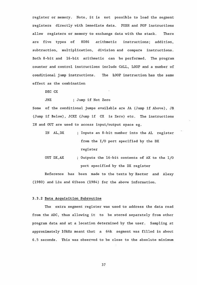
3.3.2 Data Acquisition SubroutineThe extra segment register was used to address the data read

from the ADC, thus allowing it to be stored separately from other program data and at a location determined by the user. Sampling at approximately 10kHz meant that a 64k segment was filled in about6.5 seconds. This was observed to be close to the absolute minimum

37

sample time which could be relied on to give reasonable repeatability of intermittency measurements in a typical transitional flow. It was therefore decided to use two memory segments giving a sample time of about 13 seconds.

The operation of the BLUE card is straightforward and consecutive values might be

10 PORT = &H300 20 OUT PORT,0 30 FOR i=l TO n 40 OUT PORT+2,0 50 A = INP(PORT+2)60 NEXT i

CHIP TECHNOLOGY ACM-44 interface l simple BASIC program to read n

base address = 300 (hex) selects channel 0

outputing a zero starts conversion reads value into A

The assembly language subroutine ACQ.DG reads 128k of data as 8-bit numbers at about 10kHz to provide a sample of about 13 seconds duration. This data is stored in two memory segments at physical addresses &30000 to &4FFFF and is addressed using the ES register which is set to &3000 and &4000 respectively and the offset (0 - &FFFF) is provided by the BX register. The subroutine ACQ.DG is now described in detail. Note, the channel number is selected previously by the main program.

ACQ:MOV CX,02H MOV DX,302H MOV AX,3000HSTART:ACQ: is the label for the subroutine. CX is loaded with the

number 2 since the main loop must be executed twice to read 128k of

38

data into two 64k memory segments. The value &302 stored in DX is simply the value PORT+2 used to start the conversion and to read the input value. &3000 is the value to be loaded into ES to provide the starting address for data storage and is loaded via AX since ES cannot be loaded directly with immediate data. START: is the label marking the start of the outer loop which is repeated

twice.PUSH CX MOV ES, AX MOV BX,00H MOV GX,OFFFFH C0NV_1:The current value of CX is stored on the stack and the value

&3000 is stored in ES. The BX register is set to zero and CX isloaded with &FFFF to control the loop which reads in and stores onecomplete segment of data. C0NV_1: is the label marking the startof this loop.

MOV AL,00H OUT DX,ALAL is loaded with zero and the zero is output to the address

specified by DX (ie. &302) to start the analogue to digital conversion.

PUSH CX MOV CX,24H DELAY:NOPLOOP DELAY POP CX

39

The current value of CX is stored on the stack and a new value of &24 is loaded to control a delay loop. This loop is necessary to ensure conversion is complete before the value is read in and also to control the sampling frequency. Finally, the previous value of CX is restored from the stack.

IN AL,DX MOV ES:[BX],AL INC BX LOOP C0NV_1The 8-bit digital value is read from the I/O address

specified in DX (again &302) and stored in the 8-bit AL register. This value is then stored in the "extra segment" which starts at &30000, offset by the number contained in BX. A segment override is used since data is normally stored relative to DS. The contents of BX are incremented by one to allow the next datum to be stored at the next consecutive address.

POP CXMOV AX,04000H

LOOP START RETFThe original value of CX is restored from the stack and AX is

loaded with &4000. Looping back to START: allows the second 64k segment of memory, starting at &40000, to be filled with data. The RETF instruction returns control to the main program.

The full listing of ACQ.DG in appendix 1 shows the clock cycles required for each instruction. The data acquisition loop is contained between the C0NV_1: label and the LOOP C0NV_1 instruction and contains a delay loop. The LOOP instruction requires 17 clock

40

cycles when the loop is repeated and only 5 when it is exited, thus the total number of clock cycles taken by the delay loop is

&23*(3 + 17) + 3 + 5 = 708The number of clock cycles taken by the remaining

instructions in the data acquisition loop is4 + 8 + 1 0 + 4 + 8 + 8 + 1 6 + 2 + 1 7 = 77Thus the total number of clock cycles for one execution of

the data acquisition loop is 785. The clock frequency is 8 MHz, ie. the time for one cycle is 0.125jus. Thus the time per loop is 98.125/zs giving a sampling rate of 10.19kHz.

3.3.3 Main Data Acquisition ProgramThe assembly language routine described in the previous

section is responsible for reading a succession of data from an ADC, at high speed, and storing the data in the computers RAM. To obtain a boundary layer profile, measurements must be made from as close to the plate as possible out to the freestream. The probe datum was set manually using a scaled block placed behind the probe and viewed through a cathetometer and was normally set at 0.5mm above the plate. The main program, which is written in BASIC, controls the movement of the probe, from the datum to the freestream, and records its position at each step. It also calls the data acquisition subroutine, transfers the data from RAM to thehard disc and stops the traverse after the probe is outside theboundary layer.

The signal from the hot wire anemometer was connected to channel zero on the card and the signal from the sweep drive unit was input to channel two. The digital output channel zero is

41

connected to the switch which controls the sweep drive unit. Outputing a "1" closes the switch and stops the SDU while outputing a "0" opens the switch causing the stepper motor to move the probe. The stepper motor on/off interface is shown in fig 3.6.

The data acquisition program DGDATA5.BAS is listed in appendix 1 and the main features are described here.

PORT = &H300 OUT PORT+2,&H12 OUT PORT+3,1The base address is set to 6ch300 and the "command byte" is

set at &hl2. The command byte controls the various A/D functions and in the case of the ML-16 card also selects the channel number for analogue input. Fig 3.7 shows the functions of the command byte. Setting it to &H12 selects channel 2, analogue input is unipolar in the range O-lOv and conversion is started by writing to PORT+O. The third command outputs a digital "1" to ensure that the probe does not move before the first reading is taken.

After inputing initial data such as atmospheric temperature and pressure and the initial location of the probe the data acquisition loop is entered (at line 5). A loop reads 500 values from channel two and takes the average to obtain the probe position.

OUT PORT+2,&H10 CALL ACQ SUB ACQ INLINE 4INLINE

END SUBThe first two commands select channel two and transfer

42

control to the assembly language routine. The ^INLINE is a so called metastatement which controls the compiler during compilation of the program.

CALL TOTALCl = PEEK(&HA000)C2 = PEEK(&HA001)C3 = PEEK(&HA002)C4 - PEEK(&HA003)TOTAL = C4*(224) + C3*(23<}) + C3*256 + Cl MEAN = TOTAL/(65535*";Another assembly language subroutine called TOTAL, which is

described in the next section, is called. This subroutine sums all the values which have been read in and stores the result as a 32-bit number in locations &HA000 - &HA003 in the current datasegment. This total is retrieved using PEEK commands, converted to a decimal number and divided by the number of points to obtain the mean value.

DEF SEG=&H3000BSAVE FILE|+STR$(2*N-1),0,&HFFFF DEF SEG=6cH4000BSAVE FILE$+STR$(2*N),0,&HFFFF DEF SEGThe DEF SEG command defines the data segment to be used by

various commands such as BLOAD and BSAVE. The BSAVE command saves a memory range of up to 64k to disc. For example if N=1 the data contained in memory locations &H30000 to &H3FFFF would be saved in the file FILE4 1 and the data contained in locations &H40000 to

&H4FFFF would be saved in the file FILE£ 2. Thus each 128k sample

43

is stored in two disc files. The BSAVE command is very quick, transferring 128k of data from memory to disc in about 2 seconds.

The section of code headed "test for profile complete" causes the loop to be exited if three consecutive values of mean velocity are within ±0.5% of each other. If the loop is not exited the probe is raised in the boundary layer and the loop repeated. The probe is moved by outputing a digital "0" and pausing using the DELAY command, before sending out a digital "1" to stop the probe. Since the velocity varies most rapidly close to the plate smaller steps were taken for the first six points. To avoid excessive numbers of points in a traverse the step length was increased after six points and again after twelve points. Finally initial data and the probe position data are written to a separate file.

3.4 SIGNAL CONDITIONINGTwo signals are required to be recorded by the computer ie.

the linearised hot wire signal and the output voltage from the sweep drive unit. To ensure that the ADC is used to its full capability the maximum reading expected from each instrument must be conditioned to approximately lOv. Both signals were passed through a FYLDE modular instrumentation rack which contained xO.l and xl switched gains with a xlO variable control and a digital display.

The hot wire signal was linearised such that the voltage output was equivalent to l/10th of the fluid velocity eg. 2v = 20m/s. The maximum velocity expected in the planned experiments was about 15m/s. It was decided to allow a maximum of 20m/s to be equivalent to 250 bits giving a calibration constant of 0.08. This

44

was particularly convenient when using the ACM-44 card where 250 bits corresponded to exactly lOv requiring an amplification of exactly 5. The amplification was adjusted when the ACM-44 card was replaced to retain the calibration constant.

The position of the probe above the plate is determined from the output voltage of the DISA 55D35 sweep drive unit. The output is made proportional to the linear displacement of the hot wire probe via a stepper motor and a traverse mechanism. Calibration of the sweep drive unit, fig 3.8, gives a linear relationship between the voltage and the displacement. The calibration constant was found to be 0.2022 mm/bit.

45

PC/XT/AT Port Map I/O Address MapAddress000-01F020-03F040-05F060-06F070-07F080-09F0A0-0BF0F00F10F8-0FF1F0-1F8200-207278-27F2F8-2FF300-31F360-36F378-37F380-38F3A0-3AF3B0-3BF3C0-3CF3D0-3DF3F0-3F73F8-3FF

DMA Controller 1, 8237A-5 Interrupt Controller 1, 8259A Timer, 8254Keyboard Controller, 8742; Control Port B RTC and CMOS RAM, NMI Mask (Write)DMA Page Register (Memory Mapper)Interrupt Controller, 8259 Clear NPX (80287) Busy Reset NPX, 80287Numeric Processor Extension, 80287 Hard Disk Drive Controller ReservedReserved for Parallel Printer Port 2 Reserved for Serial Port 2 Reserved ReservedParallel printer Port 1Reserved for SDLC Communucations, Bisynchronous 2Reserved for Bisynchronous 1ReservedReservedDisplay Controller Diskette Drive Controller Serial Port 1figure 3.1

46

Port Map (Bluechip Technology ACM-44 card)BASEBASE+2BASE+3BASE+4BASE+5BASE+6BASE+7BASE+8BASE+9BASE+10BASE+11

= Analogue Input Channel Select = Analogue Input Value (READ)= Start Conversion (WRITE)= Timer control = Analogue Output Channel 0 = Analogue Output Channel 1 = Analogue Output Channel 2 = Analogue Output Channel 3 = Digital I/O Port A = Digital I/O Port B = Digital I/O Port C = Digital Port control

figure 3.2

47

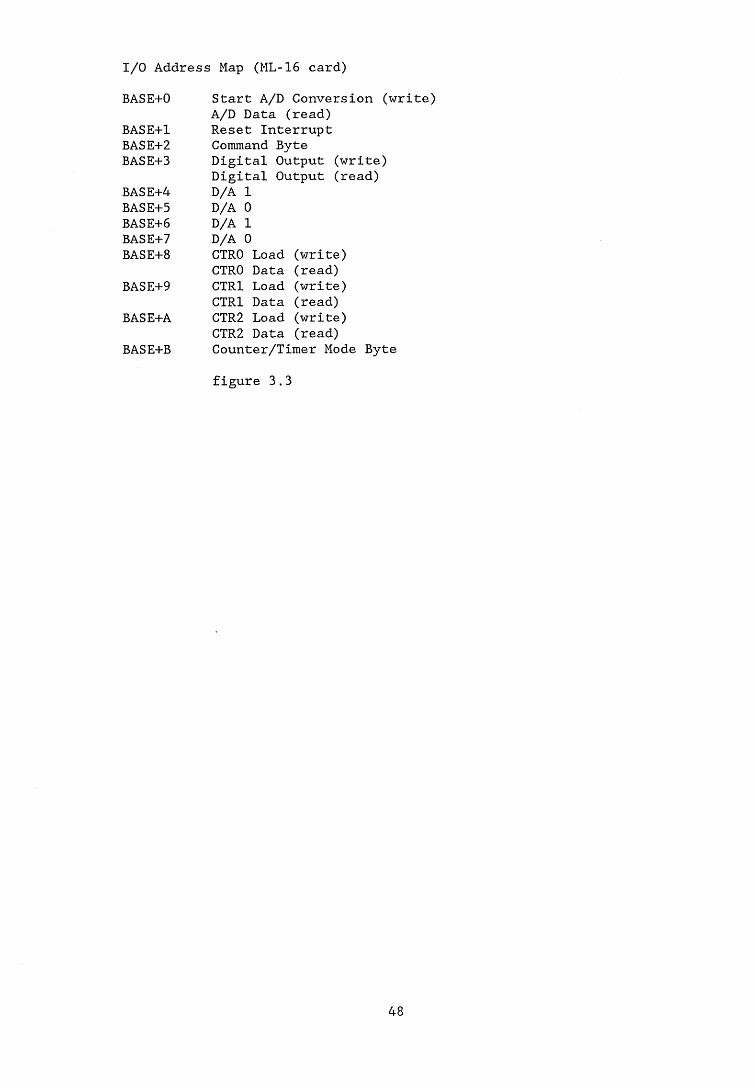
I/O Address Map (ML-16 card)BASE+OBASE+1BASE+2BASE+3BASE+4BASE+5BASE+6BASE+7BASE+8BASE+9BASE+ABASE+B

Start A/D Conversion (write) A/D Data (read)Reset Interrupt Command Byte Digital Output (write) Digital Output (read)D/A 1 D/A 0 D/A 1 D/A 0CTRO Load (write)CTRO Data (read)CTR1 Load (write)CTR1 Data (read)CTR2 Load (write)CTR2 Data (read) Counter/Timer Mode Bytefigure 3.3

48

Data Registers

AX

BX

CX

DX

Pointer & Index Registers

Base Pointer

Stack Pointer

Source Index

Destination Index

Segment Registers

Code Segment

Data Segment

Stack Segment

Extra Segment

AH AL

BH BL

CH CL

DH DL

Accumulator

Base

Count

Data

Program Counter

Status Word

figure 3.4 8086 registers

49

segment address

4-b its>------------ *------------X

16-b its 0 0 0 0 segment address

+

16-b its o ffset

020-b its actual address

figure 3.5 memory addressing

50

reed relay

Ov

figure 3.6 stepper motor on/off interface

51

______ BIT_________7 6 5 4 3 2 1 0

CHANNEL CHANNELS/E DIFF S/E DIFF

0 0 0 0 - 0 0 1 0 0 0 - 8 40 0 0 1 - 1 - 1 0 0 1 - 9 -

0 0 1 0 - 2 1 1 0 1 0 - 10 50 0 1 1 - 3 - 1 0 1 1 - 11 -0 1 0 0 - 4 2 1 1 0 0 - 12 60 1 0 1 - 5 - 1 1 0 1 - 13 -0 1 1 0 - 6 3 1 1 1 0 - 14 70 1 1 1 - 7 - 1 1 1 1 - 15 -

INPUT RANGE * 10 = 255mV (low range)1 = 10V (high range)UNIPOLAR/BIPOLAR0 = unipolar1 = bipolarFORMAT0 = straight binary in unipolar mode0 = offset binary in bipolar mode1 = 2's complementA/D CONVERSION MODE0 = convert on write to BASE+01 = convert on A/D read

figure 3.7 command register bit assignments for the ML-16 multi-lab board

52

calibration of the sweep drive unit

Volta

e— volts

figure 3.8

CHAPTER 4

DATA REDUCTION

It has already been noted that high frequency digital sampling of an analogue signal can quickly generate large quantities of numerical data. In the present case a 13 second sample of the velocity signal requires 128k of memory and a profile consisting of up to about 28 such samples can require as much as3.5 Megabytes of space on the hard disc. Depending on the number of points per profile there is enough room to store only five or six complete profiles on the computers hard disc at any one time. To keep a complete digital record of all the flows measured would require a vast amount of storage so it was necessary to process the raw signal to reduce the data to a more manageable format. As well as the mean velocity and RMS of each sample the intermittency was calculated and, in transitional flows, the mean laminar and turbulent velocities were also determined. All processing was to be carried out digitally, however it soon became apparent that processing time could become a significant issue. For example, summing the 131,072 individual values, which make up a sample, took over two minutes using compiled BASIC ie. it could take almost an hour just to determine the mean velocity profile of one traverse. However, judicious use of an assembly language subroutine to execute the summation reduced the time from two minutes to less than two seconds thus giving more acceptable processing times. All summation procedures were programmed in assembly language with

final divisions, square root operations etc, which need to be performed only once for each sample, being programmed in BASIC for simplicity.

55

4.1 REDUCTION OF THE RAW DATAThe data reduction program DGDATA6.BAS reloads the raw data

into the computers memory and calculates the mean velocity, RMS, intermittency and the mean laminar and turbulent components of velocity. Finally, the mean data for a complete profile is saved in a new file. This data can be further processed to provide the usual integral parameters, both for the mean velocity profile and for the laminar and turbulent component profiles.

4.1.1 Mean VelocityThe first value required from the data reduction is the mean

velocity which is given by

u = Su n

The calculation of the mean velocity is greatly accelerated by the use of an assembly language routine to calculate Su. The division occurs only once and can be easily performed in BASIC with no loss of speed. The data is accessed in much the same way as it was stored by ACQ.DG in that the main loop must be executed twice to access the two segments of data. A complete listing of TOTAL.DG is contained in appendix 1 and the main aspects of the routine are detailed below.

MOV AX,00HMOV [0A000H],AXMOV [0A002H],AXThe total, 2u, is to be stored as a 32-bit number at memory

locations &A000, &A001, &A002 and &A003, relative to DS.MOV [ ] ,AX moves the low byte of AX to the address in the square

56

brackets and the high byte to address+1. These memory addresses are cleared to zero initially.

MOV DL,ES:[BX]MOV DH,00H MOV AX,[0A000H]The 8-bit value held in ES:[BX] is stored in the DX register.

The quantity currently held in addresses &A000 and &A001 is moved

to AX.ADD AX,DX MOV [0A000H],AX MOV AX,[0A002H]ADC AX,00H MOV [0A002H],AXStandard 32-bit addition is used to add the value in DX to

the running total held at addresses &A000 to &A003 and the new total is returned to the same addresses.

The main program obtains the value Su by peeking the memory locations thus

U1 = PEEK(&HA000)U2 = PEEK(&HA001)U3 = PEEK(&HA002)U4 - PEEK(&HA003)

andSu = U4*224 + U3*216 + U2*28 + U1

4.1.2 RMS SubroutineThe RMS of the velocity fluctuations is given by

57

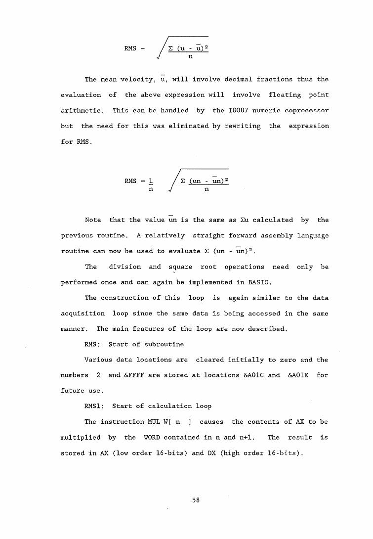
RMS S (u - u)2v n

The mean velocity, u, will involve decimal fractions thus the evaluation of the above expression will involve floating point arithmetic. This can be handled by the 18087 numeric coprocessor but the need for this was eliminated by rewriting the expression

for RMS.

RMS = 1 n

Note that the value un is the same as Eu calculated by the previous routine. A relatively straight forward assembly language routine can now be used to evaluate 2 (un - un)2.

The division and square root operations need only be performed once and can again be implemented in BASIC.

The construction of this loop is again similar to the data acquisition loop since the same data is being accessed in the same manner. The main features of the loop are now described.

RMS: Start of subroutineVarious data locations are cleared initially to zero and the

numbers 2 and &FFFF are stored at locations &A01C and &A01E for future use.

RMS1: Start of calculation loopThe instruction MUL W[ n ] causes the contents of AX to be

multiplied by the WORD contained in n and n+1. The result is stored in AX (low order 16-bits) and DX (high order 16-bits).

58

MUL W[0A01CH]MUL W[0A01EH]MOV [0A004H],AXMOV [0A006H],DXThe first instruction gives u*2, which has a maximum value of

2*255 = 510, which is stored in AX. The second MUL instruction gives u*2*&FFFF ie. the quantity un which is stored as a 32-bit number.

Before calculating (un - un) 2 the two quantities, un and un, are compared, high bytes first, to determine which is the larger. To avoid confusion with two's complement negative numbers, the smaller of the two values is subtracted from the larger to give the absolute value of (un - un). This has no effect on the final result since squaring results in a positive number anyway. 32-bit subtraction is employed and the result is stored in locations &A008 - &A00B.

The squaring routine is modified from a 32-bit multiplication routine given by Rector and Alexy (1980) which gives a 64-bit answer. The quantity S (un - un) 2 is obtained by 64-bit addition which is a simple extension to the procedure used in TOTAL.

The LOOP command failed in this program because the jump was greater than 128 hence CX was decremented explicitly and an unconditional jump was used when CX > 0.

Mean velocity and RMS values obtained digitally were compared with measurements made by analogue instrumentation over a range of flow conditions. Errors were within about one percent and were probably due to the fact that the analogue instrumentation was read manually.

59

4.1.3 Intermittency MeasurementTo discriminate between laminar and turbulent flow some

characteristic of the flow must be found which is significantly different in each type of flow. In the literature various criteria have been used as "detector functions". Corrsin and Kistler (1955) used the streamwise component of vorticity, cox , to identify turbulent and non-turbulent regions in the intermittent interface of the turbulent boundary layer. This technique however, required the use of an array of four hot wire anemometers. Kovasznay et al (1970) used 3u/3y, which is effectively a measure of the spanwise vorticity, , as the basis of detection. The flow was considered to be turbulent if either 32 u/3y3t or 33 u/3y3t2 exceeded set threshold values. These quantities are not necessarily zero in non-turbulent flow and can cross zero in turbulent flow therefore some smoothing was applied to average out these errors. Here two hot wires, separated by 5mm in the y direction, were required to measure 3u/3y. Kaplan and Laufer (1969) used a digital computer to process their data and based their detector function on the short time variance of 3u/3t. Murlis et al (1982) used the product uv as the detector function. In a similar procedure to Kovasznay et al (1970) turbulence was registered if either the first or second time derivatives of uv exceeded separate thresholds. Measurement of uv however, necessitates the use of a cross wire probe which is impractical in thin boundary layers.

Using a single wire probe, it is only possible to consider the level of the signal or its variation with respect to time as a potential detector function. A turbulent signal consists of higher frequency, higher amplitude fluctuations than a laminar signal and

60

it would be expected therefore that the rate of change of the signal, with respect to time (3u/3t), would be greater, on average, in a turbulent region. It was decided to investigate both 3u/3t and 3 2 u/3 t2 as possible means of discriminating between laminar and turbulent flow. As with other criteria however, both 3u/3t and 32 u/3t2 can be non zero in non-turbulent flow while momentary zero values can occur in turbulent flow. To reduce these discrepancies the signal was digitally rectified and smoothed.

The rate of change of u with respect to time at a point i, can be represented by the forward difference approximation

3u = u'ui - ui (4.1)3t At

where u\, and u- are two consecutive data points and At is the sampling period. The signal is rectified by taking the absolute value of expression (4.1) and smoothing is achieved by summing over a number of points, n. The smoothing period, nAt, should remain small relative to the average time duration of a turbulent spot or laminar region. Thus

nF(t) - _1_ 2 |u-w 1 - u-J (4.2)

nAt i=l

Since At is constant a function Sl(t), which is proportional to a smoothed and rectified 3u/3t signal can be given as

nSl(t) = 2 |u-tM - u-J (4.3)

i=l

Similarly a function S2(t), which is proportional to a

61

smoothed and rectified 32u/3t2 signal is given by

nS2(t) = 2 |u-lM - 2uu + u Ul | (4.4)

i= 2

Sufficient smoothing must be applied to the detector functions to allow a threshold to be fixed which will allow an intermittency of 1 to be recorded in a fully turbulent boundary layer and zero to be recorded in laminar flow or the freestream. Figure 4.1 shows intermittencies obtained using Sl(t) in a fully turbulent boundary layer and the freestream. Smoothing over 10 points and 2 0 points has been used and the graph has been normalised by plotting on a base of threshold value divided by the number of smoothing points. Increased smoothing appears to have little effect on intermittency measurement in the freastream with both 1 0 and 2 0 point smoothing behaving almost identically as the threshold value is decreased. In the fully turbulent boundary layer, increasing the smoothing period slightly reduces the effects of momentary zero values of Sl(t). Smoothing of 15 points, ie. n = 14, was found to be about the minimum reliable value for bothSl(t) and S2(t) and increasing this had little effect on the results other than to increase computing time. It is clear from figure 4.1 that there is a range of possible threshold values which will satisfy the above criterion. The optimum threshold was found to be about Sl(t) = S2(t) = 26.

The most accurate identification of the interface between a turbulent spot and the surrounding laminar flow was obtained if the smoothing was centered about the point under consideration eg. if the function Sl(t), defined in equation 4.2, exceeded the threshold

62

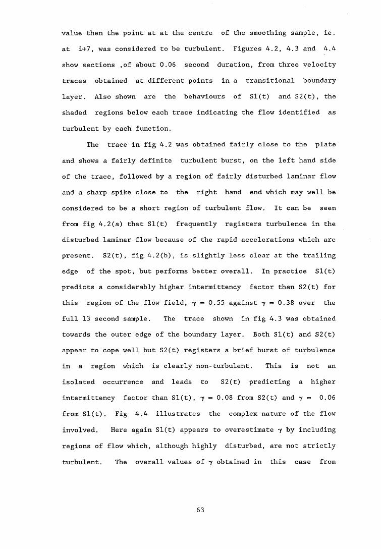
value then the point at at the centre of the smoothing sample, ie. at i+7, was considered to be turbulent. Figures 4.2, 4.3 and 4.4 show sections ,of about 0.06 second duration, from three velocity traces obtained at different points in a transitional boundary layer. Also shown are the behaviours of Sl(t) and S2(t), the shaded regions below each trace indicating the flow identified as

turbulent by each function.The trace in fig 4.2 was obtained fairly close to the plate

and shows a fairly definite turbulent burst, on the left hand side of the trace, followed by a region of fairly disturbed laminar flow and a sharp spike close to the right hand end which may well be considered to be a short region of turbulent flow. It can be seen from fig 4.2(a) that Sl(t) frequently registers turbulence in the disturbed laminar flow because of the rapid accelerations which are present. S2(t), fig 4.2(b), is slightly less clear at the trailing edge of the spot, but performs better overall. In practice Sl(t) predicts a considerably higher intermittency factor than S2(t) for this region of the flow field, 7 = 0.55 against 7 = 0.38 over the full 13 second sample. The trace shown in fig 4.3 was obtained towards the outer edge of the boundary layer. Both Sl(t) and S2(t) appear to cope well but S2(t) registers a brief burst of turbulence in a region which is clearly non-turbulent. This is not an isolated occurrence and leads to S2(t) predicting a higher intermittency factor than Sl(t), 7 = 0.08 from S2(t) and 7 = 0.06 from Sl(t). Fig 4.4 illustrates the complex nature of the flow

involved. Here again Sl(t) appears to overestimate 7 by including regions of flow which, although highly disturbed, are not strictly turbulent. The overall values of 7 obtained in this case from

63

Figures 4.2 to 4.4 show only a small sample of the variety of flow conditions which occur in the present set up but the features observed appear to apply generally in that neither Sl(t) nor S2(t) is entirely satisfactory as a turbulence detector function throughout the complete transition region. Both Sl(t) and S2(t) rise rapidly immediately turbulence is encountered but, because of the smoothing, the functions have a finite slope. This means that the intermittency recorded will depend, to some extent, on the level of the threshold. It is desirable to set the threshold as low as possible to register turbulence as soon as it occurs but lowering the threshold leads to an increase of false readings in the non turbulent flow, as previously described. This was overcome by registering turbulence only when Sl(t) and S2(t) exceeded their threshold values. This ensures that turbulence is registered as soon as both SI and S2 begin to rise rapidly but eliminates errors due to minor excursions, above the threshold, of Sl(t) or S2(t) individually. Figures 4.5 to 4.7 repeat the previously described signals and show the turbulence registered using an Sl(t) AND S2(t) criterion.

The use of an arbitrary fixed threshold is satisfactory in the present application where the transition region is fairly short and external conditions do not vary excessively over the transition region. It is clear however, that the optimum threshold may vary from flow to flow and possibly from location to location in a particular flow. Boundary layer transition under an imposed adverse pressure gradient is particularly complex and the measurement of intermittency in such a flow is subjective. While

Sl(t) and S2(t) were 0.46 and 0.36 respectively.

64

turbulent regions and obviously non-turbulent regions can be defined there is a proportion of the flow which cannot be unambiguously assigned to either category. The non-turbulent flow is in a disturbed state and exhibits high amplitude, low frequency fluctuations and occasional bursts of relatively high frequency sinusoid like fluctuations. Using a single wire signal, ie. direct measurement of u, and its time derivatives is the simplest approach to conditional sampling. The evidence presented in figures 4.5 to 4.7 suggests that the technique developed is no less reliable than any of the more complex methods which have been used.

The program DATA9.BAS, see appendix 1, allows a 13 second sample to be taken and examined visually, on the computer screen, in sections of 640 points, ie. about 64mseconds, at a time. Since only 640 points are considered at any one time all calculations are executed in BASIC. The variables VLAM and VTURB, which will hold the sum of the laminar and turbulent velocities respectively, and CLAM and CTURB, which will hold the number of laminar and turbulent points, are initially set to zero. Fifteen consecutive points are loaded into the array VEL( ) using the PEEK command and the variables SUM1 and SUM2, ie. Sl(t) and S2(t), are set to zero. The values of SUM1 and SUM2 are calculated and if both exceed 26 the appropriate point is added to VTURB and CTURB is incremented by one. Otherwise the point is added to VLAM and CLAM is incremented by one. Finally the mean laminar and turbulent velocities are calculated and the intermittency is given by the number of turbulent points divided by the total number of points.

Again it is necessary to use an assembly language routine in the calculation of the intermittency and mean laminar and turbulent

65

components of velocity for a complete sample. This assembly language subroutine determines the intermittency and the values equivalent to VLAM, VTURB, CLAM and CTURB. The divisions required to obtain the mean laminar and turbulent velocities are again performed once each in BASIC. The subroutine follows exactly the same logic as the previously described BASIC program.

4.2 REDUCTION OF MEAN VELOCITY PROFILESThe program ANLYS4.BAS reduces the mean velocity data from

laminar, turbulent and transitional boundary layers to give the usual integral parameters. In the case of transitional boundary layers the mean laminar and turbulent component profiles are also reduced separately. The boundary layer thickness, 8, is estimated from the mean profile by linear interpolation and is taken to be the point where u = 0.995U . The program also calculates the "near wall" intermittency which is the most commonly used factor in describing transitional boundary layers. The intermittency remains more or less constant up to about y/8 =0.4 and the near wall intermittency was taken to be the average for all points below this value. Following the approach of Gardiner (1987) the laminar analysis, described in section 4.2.1, was used to reduce mean transitional profiles when 7 < 0.5 and the turbulent analysis, described in section 4.2.2, when 7 > 0.5. A typical printout from the analysis program is shown in fig 4.8.

4.2.1 Reduction of Laminar Mean Velocity ProfilesBoth Gardiner (1987) and Fraser (1979) obtained the integral

parameters for laminar velocity profiles by direct integration of a

66

polynomial which was fitted through data points of u/U against y/8 using a least squares technique. Fraser (1979) used a fourth order polynomial while Gardiner (1987) found that a third order polynomial was sufficient. The present work involved the measurement of inflectional and separating laminar velocity profiles and it was found that fitting a polynomial to the data was unreliable in these cases. To obtain more reliable integration of the laminar profiles a technique described by Coles and Hirst (1968) and used by Fraser (1979) and Gardiner (1987) for turbulent boundary layers was adapted.

The procedure was to fit a parabola through three consecutive points and compute the integrals from the first to the second and from the second to the third using Simpson's Rule. The central point is then moved out one and the process repeated’. The two values which are obtained for each interval, other than the first and last, are then averaged to provide an element of smoothing. The integrals of

which are obtained are appropriately combined to give the required integral parameters.

In a laminar layer the shear stress is directly proportional to the rate of strain ie.

f ] , (‘ ' 4 - ) , ( 4 - ) ’ * " a ( 4 - ) '

T = fl( <9u 1l 3y J (4.5)

By assuming a linear profile between the wall and the first data point an estimate of the wall shear stress could be made. Since the first data point is always 0.5mm above the surface this

estimate will be unreliable in thin boundary layers and also as separation is approached.

4.2.2 Reduction of Turbulent Mean Velocity ProfilesTurbulent boundary layer velocity profiles were reduced using

the analysis of Coles (1968), as applied by Coles and Hirst (1968) to the data presented at the Stanford conference. Fig 4.9 shows the structure of a typical turbulent boundary layer which consists of a thin viscous sublayer, "so-called" inner and outer layers and an irregular but sharp interface with the freestream. In the viscous sublayer, viscous forces dominate and the mean velocity profile can be approximated by

u = yux (4.6)U-f v

where u^P

■t*This equation is often written as u = yColes (1956) used two similarity laws, the law of the wall

and the law of the wake, to develop an empirical equation for the mean velocity profile ie.

u+ = f(y+) + II W f y ) (4.7)* l s J

The law of the wall (the function f(y+)) has the form f(y+) = _1_ In y+ + C (4.8)

Kwhere k and C are empirical constants. Equation 4.8 applies

outside the viscous sublayer and the buffer layer, ie. for y+ > 50The values of k and C are slightly controversial because of scatter in the data. Coles (1968) used the values /c=0.41 and C=5.0 but

68

since the present investigation was concerned with low Reynolds number turbulent boundary layers the value of C = 5.2, as suggested by Murlis (1975) and used by Fraser (1979) and Gardiner (1987) among others, was adopted.

The law of the wake describes the deviation of the velocity, above the law of the wall, in the outer layer. Coles (1968) noted that the velocity deviations were a single wakelike function when normalised by the maximum deviation at y = 8 . The wake function, W, is approximately antisymmetric about y = 8/2, W = 1 therefore Coles proposed the following curve fit.

W

Equation 4.7 written in full is thereforeu = 1 In yurut k L v

+ C + 211 sin2K

(4.9)

(4.10)

where II is called the wake parameter. At the edge of the boundary layer equation 4.10 becomes

U = _1_ lnl" 8ux 1 + C + 2n (4.11)ut K L u K

This equation relates the three parameters ux ,8 and n and can beused to determine any one if the other two are known.

The law of the wall, eqn 4.8, is assumed to be valid in theregion y+ > 50 and y/S < 0.2 following the suggestion of Murlis etal (1982) to allow for the low Reynolds number flows in the presentwork. For each point within the specified region equation 4.8 issolved iteratively for ur. The averaged value of ut from all suchpoints is then taken to be the representative value for thevelocity profile under consideration. With 8 and ur now known the

69

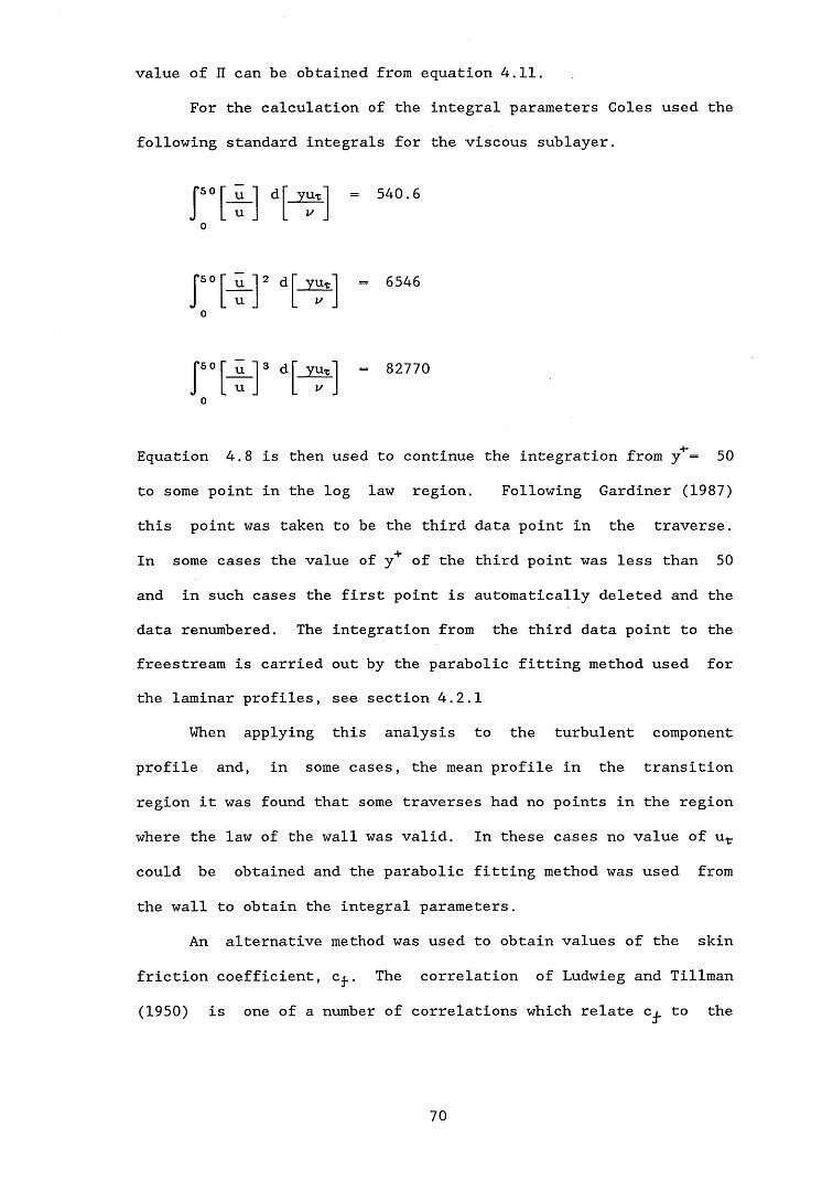
For the calculation of the integral parameters Coles used the following standard integrals for the viscous sublayer.

value of II can be obtained from equation 4.11.

540.6

6546

82770

Equation 4.8 is then used to continue the integration from y** = 50 to some point in the log law region. Following Gardiner (1987) this point was taken to be the third data point in the traverse. In some cases the value of y of the third point was less than 50 and in such cases the first point is automatically deleted and the data renumbered. The integration from the third data point to the freestream is carried out by the parabolic fitting method used for the laminar profiles, see section 4.2.1

When applying this analysis to the turbulent component profile and, in some cases, the mean profile in the transition region it was found that some traverses had no points in the region where the law of the wall was valid. In these cases no value of ut could be obtained and the parabolic fitting method was used from the wall to obtain the integral parameters.

An alternative method was used to obtain values of the skin friction coefficient, c^. The correlation of Ludwieg and Tillman (1950) is one of a number of correlations which relate c^ to the

70

shape factor, Htv and the momentum thickness, 9, ie.cf = 0.246R©“°•268 exp(-1.561H,^) (4.12)

The wall shear stress, rw , can also be calculated from the value of u^ obtained from the law of the wall analysis ie.

r w = /m-t2 (4.13)and the skin friction coefficient follows from

c* - _2tw - 2f_otl2 (4.14)pU2 { U J

4.2.3 Transitional Mean Velocity ProfilesDhawan and Narasimha (1958) represented the mean velocity in

a transitional boundary layer by the intermittency weighted average of the mean laminar and turbulent component velocities, ie.

= (l-7 )uu + 7 U-r (4.15)They also stated that although 7 varied across the boundary layer, the value measured close to the wall gives sufficiently accurate results for the whole profile. The effect of 7 variation with y was briefly investigated during the present work. Klebanoff (1955) measured the intermittency in a boundary layer in a zero pressure gradient flow and White (1974) proposed the following curve fit.

7 - [1 + 5(y/5) 6 ] “ 1 (4.16)Equation 4.16 was compared with some of the data of Gardiner

(1987). Fig 4.10 shows a set of intermittency profiles from a transitional boundary layer in a zero pressure gradient flow. The similarity of the curves is apparent. Each set of data was normalised by the "near wall" intermittency and replotted. The data was found to collapse on to the curve as shown in fig 4.11. This suggested that equation 4.16 could be used, along with the near wall intermittency, to describe the intermittency variation

71

with y in transitional boundary layers. All intermittency profiles measured during the present work were normalised and plotted against White's curve fit and good agreement was found in most cases. Two typical examples are shown in figures 4.12 and 4.13. This, along with some of the results of Gardiner (1987), indicate that equation 4.16 can also be applied, at least as a first approximation, to turbulent flows in adverse pressure gradients.

Using equation 4.15 Dhawan and Narasimha (1958) showed that the displacement thickness in the transition region was given by

C - (1 ~r>«* + yS* (4-17)

They also calculated the corresponding expressions for 6 and H although these turn out to be more complex. Taking intermittency to be a function of x and y, ie.

7' = 7 7y (4.18)where 7y = [1 + 5(y/5)6]“1it can be shown that

8 = - 7 & f1 1 - u»-/u + 7 gf1 1 - u-r/U dy3 (4.19)r J [1 + 5/36] J f l + 5/36 ]0 0

where /? = y/5In the transition region equations 4.17 and 4.19 were both

used to obtain a value for the transitional displacement thickness from the laminar and turbulent values. When these were compared with the value obtained by reducing the mean velocity profile equation 4.19 was found to be much more accurate. This improvement might have been expected since the measured turbulent displacement thickness is based on measurements which isolate the completely turbulent flow. However methods which use equation 4.17 and the

72

corresponding expressions for momentum thickness and shape factor, see for example Fraser and Milne (1986) or Fraser et al (1987), are not incorrect for the following reason. These methods use standard integral techniques to provide laminar and turbulent values in the transition region. Most integral techniques for turbulent boundary layers take the intermittent outer region into account, eg. through the law of the wake (eqn. 4.10). Thus the near wall intermittency is appropriate when combining the laminar and turbulent values.

The previously described methods for obtaining the skin friction were used separately for the laminar and turbulent profiles and could be combined to give a transitional value using a near wall intermittency weighting, ie.

( O tr= (1 - 7 ) < O u + 7(0-r (4.20) as suggested by Dhawan and Narasimha (1958). Again this is physically more realistic than simply using a laminar analysis in a

predominantly laminar boundary layer and a turbulent analysis in a predominantly turbulent boundary layer.

4.2.4 Start and End of TransitionVarious techniques have been used in the past to determine

the locations of the start and end of transition. This has undoubtedly contributed to the considerable scatter in transition data. During the present work the start and end of transition were determined from intermittency measurements with two techniques being considered. One method was to define the start of transition as the point where the near wall intermittency was 0 . 0 1 and the end of transition as the point where it was 0.99, the two points being estimated from a plot of the complete intermittency distribution.

73

Although this method has been popular it is still very difficult to locate these points accurately. An alternative approach was that used by Narasimha (1985) and also by Dey (1988). The function F(7 ),

given byF(7) = [-ln(l - 7 )]°* 5 (4.20)

varies linearly with x and the start of transition is obtained by linear interpolation to F(7 ) = 0. This method leads to different measured values of 7 at the start of transition however. Because of the variety of techniques available to locate the start and end of transition a useful measure of the transition length is the distance between the points of 0.25 and 0.75 intermittency which can be more readily located. This value is given the symbol A and has been described in section 1.3.

74

Data for Threshold Setting

interm ittencyi _ n n n n A a~ □

0.8

0.6 H

0.4 -

0.2 -i

0

C>V 7

V7

V

^ -A

A

□

A

□

— I3.50 0.5 1 1.5 2 2.5 3

threshold/no. of smoothing points

a 10 pts (tf -1) o 1 0 pts n-o)

A 20 pts (Y -1) v 20 pts ( Y»0)

figure 4.1 measurements m a fully turbulent b.I. and the freestream

75

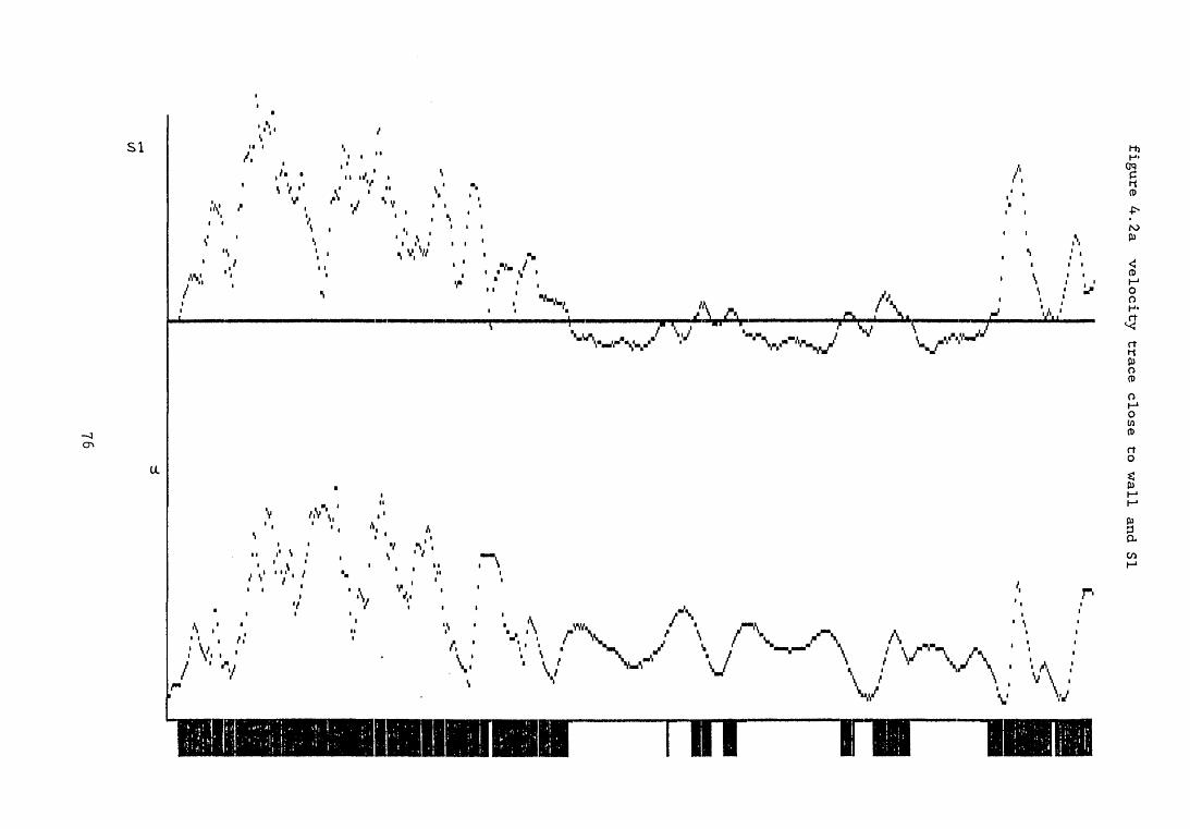
figure 4.2a velocity trace close to wall and SI

76

figure 4.2b velocity trace close to wall and S2

77

figure 4.3a velocity trace near b.l. edge and SI

78

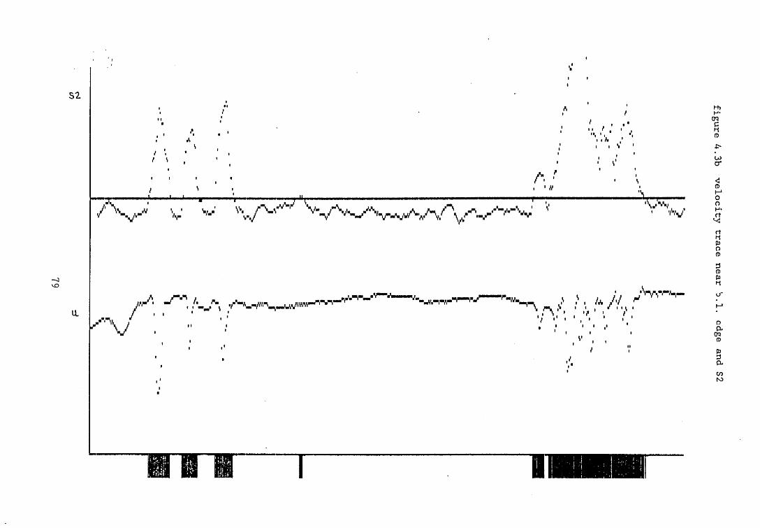
figure 4.3b velocity trace near b.l. edge and S2

79

figure 4.4a intermediate velocity trace and Si

80

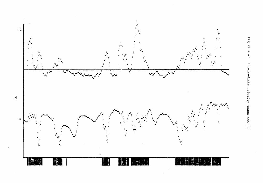
figure 4.4b intermediate velocity trace and S2

S1/S2. figure 4.5 velocity trace close to wall with SI AND S2

C_

A

J1

5 ■ a

823

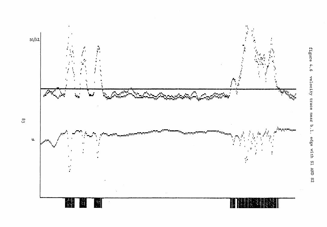
S1/S2

figure 4.6 velocity trace near b.l. edge with SI AND S2

83

S1/52 figure 4.7 intermediate velocity trace with SI AND S2

-

’-'-

A>

r■

K

«f.'

r■i:

_p-

d

84

F I L E N A M E t e s t l \ t 1668

b .1. thickness Intermittency freestream velocity Reynolds number (x)

Simpsons rule is used from the wall

TRANSITIONAL B.L. PARAMETERS

PARAMETER LAMINAR TURBULENT

disp thk (m m ) 1.876 1.821mom thk (m m ) .591 .899energy thk (mm') .911 1.445H12 3.176 2.025H32 1.543 1.607Rd isp 1717 1667Rmom 541 823Cf 4.03E-004 --Cf Lud/till -- 1 .724E-003Cf Log-plot -- 0TO 4.7E-002 . 102Wake par. -- 0

COMBINED PARAMETERSa) Dhawan and Narasimha dislacement thickness 1.853 m m

b) Modified intermittency displacement thickness 1.805 m m

TRANSITIONAL MEAN PROFILE

LAMINAR BOUNDARY LAYER PARAMETERS

displacement thickness momentum thickness energy thickness shape factor 12 shape factor 32displacement thickness Reynolds no momentum thickness Reynolds no to cf

figure 4.8 sample output from analysis program

1.811 m m.685 m m1.061 m m2.6461.551657626 ^ 9E-002 n /m 7.65E-004

5 . 0 1 m m.41114.06 m /s 611355.38

85

y = 1.25 y = 5

y = 0.45 y = 0.25

y < 0.015inner layer

7 ------- 7 --------/ t \ / / ~r~ / / - / / ..... 7 / 7\ ___ viscous sublayer

figure 4.9 schematic representation of a turbulentboundary layer

86

5 ( y / £ ) 6 ] 1 (equation 4.16) figure 4.10 transitional intermittency data from Gardiner (1987)

oa

■f+

>o87

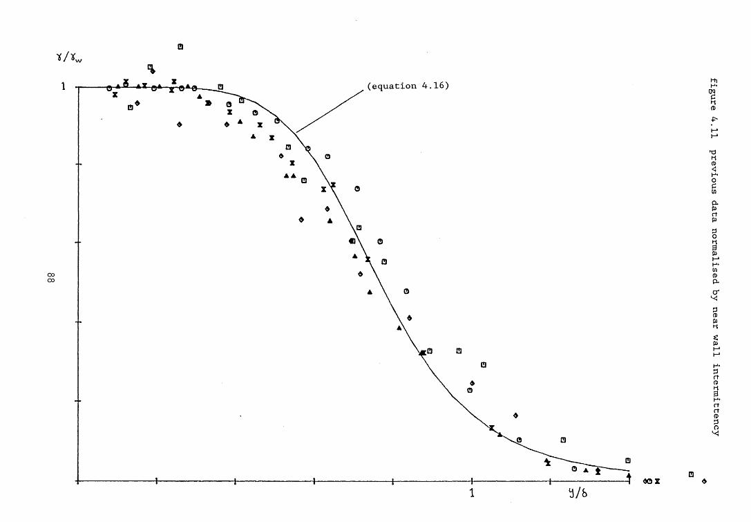
figure 4.11 previous data normalised by near wall intermittency

oBN8

>»88

y /d e lta1

figure 4.12 example of present data plotted against equation 4.16

(near wall intermittency - 0.65)

89

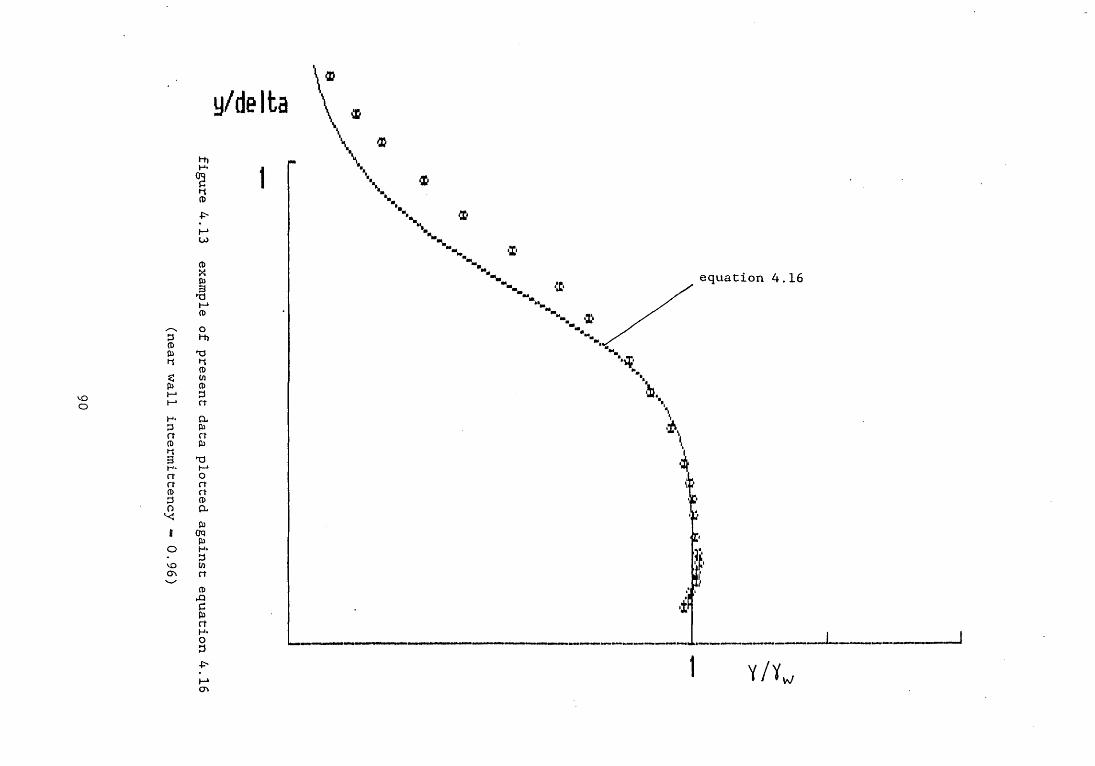
y/delta

>-

figure 4.13 example of present data plotted against equation 4.16

(near wall intermittency * 0.96)

90

CHAPTER 5

DISCUSSION OF EXPERIMENTAL RESULTS

Detailed measurements were made of the boundary layer which developed in a simulated turbine blade flow. A velocity distribution typical of the suction surface of a forward loaded, or "squared-off" design, aerofoil was reproduced in a low speed wind tunnel. Particular attention was paid to the transition region. Conditional sampling techniques were used to investigate the behaviour of the laminar and turbulent components of the flow. One feature of interest was the possibility of intermittent separation,

as described in chapter one, which was first raised by Gardiner (1987). The effect of varying freestream turbulence on the location and extent of transition was also investigated. Intermittency data collected showed that the concept of statistical similarity of transition regions was also applicable to the present case which involved fairly severe adverse pressure gradients.

The boundary layer was allowed to develop naturally from the leading edge of the smooth aluminium plate and transition was considered to be influenced mainly by the freestream turbulence level and the streamwise pressure distribution. It was found that three of the existing turbulence generating grids all produced a turbulence level at the inlet of about 1%. Only the coarsest grid produced a higher turbulence level of about 1.5%. A further grid, of similar design, which gave an inlet turbulence level of about 2% was constructed.

In common with Gardiner (1987) and other workers it was assumed that the turbulence was isotropic ie.

Tu = J u'2 + v*2 + w'2 = J xx12 (5.1)3 U U

No measurements of v' and w' were made to justify this but Blair

92

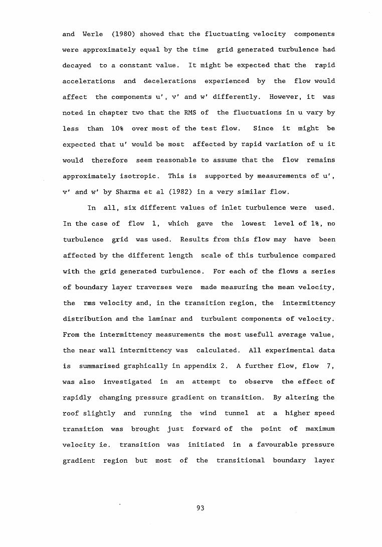
and Werle (1980) showed that the fluctuating velocity components were approximately equal by the time grid generated turbulence had decayed to a constant value. It might be expected that the rapid accelerations and decelerations experienced by the flow would affect the components u' , v' and w' differently. However, it was noted in chapter two that the RMS of the fluctuations in u vary by less than 10% over most of the test flow. Since it might be expected that u' would be most affected by rapid variation of u it would therefore seem reasonable to assume that the flow remains approximately isotropic. This is supported by measurements of u', v' and w' by Sharma et al (1982) in a very similar flow.

In all, six different values of inlet turbulence were used. In the case of flow 1, which gave the lowest level of 1%, no turbulence grid was used. Results from this flow may have been affected by the different length scale of this turbulence compared with the grid generated turbulence. For each of the flows a series of boundary layer traverses were made measuring the mean velocity, the rms velocity and, in the transition region, the intermittency distribution and the laminar and turbulent components of velocity. From the intermittency measurements the most usefull average value, the near wall intermittency was calculated. All experimental data is summarised graphically in appendix 2. A further flow, flow 7, was also investigated in an attempt to observe the effect of rapidly changing pressure gradient on transition. By altering the roof slightly and running the wind tunnel at a higher speed transition was brought just forward of the point of maximum velocity ie. transition was initiated in a favourable pressure gradient region but most of the transitional boundary layer

93

developed in a region of adverse pressure gradient. This did not constitute a complete study but the results are considered in this chapter.

5.1 START OF TRANSITIONThe linearised stability theory has proved successful in

predicting the point of instability ie. the location at which a laminar boundary layer first becomes unstable. Following the initial amplification of two dimensional Tollmein-Schlichting waves the flow becomes increasingly complex, as outlined in chapter one, before the appearance of turbulent spots which effectively mark the start of transition to a fully turbulent boundary layer. Theoretical analysis is not readily extended to predict the onset of turbulence. Also, the linear stability theory is not strictly applicable to flows with high freestream turbulence hence the multitude of correlations and semi-theoretical prediction methods which exist. Transition data exhibits considerable scatter which, as was noted in the previous chapter, can be partly attributed to the variety of techniques used to detect the onset of transition. For example Hall and Gibbings (1972) and others have used the surface pitot method. Here, the start and end of transition are located by maximum and minimum readings from a surface pitot. Abu-Ghannam and Shaw (1980) used hot wire instrumentation and used the variation of the ratio of surface velocity to reference velocity to determine the start and end of transition Reynolds numbers. For the present work the more direct approach of using intermittency measurements to locate the transition region was adopted.

94

Two techniques for determining the location of the start of transition have been considered. The first was the method used by Fraser et al (1988) whereby the start of transition is defined as the point where the flow becomes 1% turbulent, ie. the intermittency reaches 0 .01, and the end of transition is the point where the flow becomes 99% turbulent. These points can be reasonably well estimated from a plot of intermittency against streamwise location. Fraser et al (1988) noted that this technique could be expected to give the start of transition earlier than that of Abu-Ghannam and Shaw (1980) under the same experimental conditions.

Alternatively a technique first introduced by Narasimha (1957) was used to locate the start of transition. The function

F(7),

F<7) - [-ln(l - 7)]0*5 (4.20)

has been shown to vary linearly with x in zero pressure gradient flows. The start of transition location, x^, is obtained by extrapolating to F = 0 from the best fit straight line through the data. This method can give various values of intermittency at the start of transition but Narasimha (1985) suggests that the xt given by this method is the most appropriate since it is the effective origin of the turbulent boundary layer which follows the transition region. Narasimha (1985) has observed that pressure gradients can affect the linearity of F with x, particularly if they are applied close to xt.

Table 5.1, on page 112, gives details of the experimental

95

flows and summarises the transition data. Figures 5.1 to 5.6 show the present intermittency data plotted in the form suggested by Narasimha and described above. It can be seen that the lower turbulence flows, ie. flows 1 to 4, give good straight lines and x can be readily obtained. Flow 5 shows a kink and can be best fit by two straight line segments while flow 6 appears to be best fit by three straight line segments. These kinks were described as "subtransitions" by Narasimha (1985). Thus there is some ambiguity about the values of xt for flows 5 and 6 . In all cases is larger than xs.

The velocity gradient is fairly constant over the range of locations of the start of transition at about -6.15 ms " !/m (see figure 2.2). This value was used to obtain values for the pressure gradient parameter, m, at the start of transition. As can be seen from table 5.1 the values of m at the start of transition are very low indicating that laminar separation may be imminent or indeed have already occurred. In fact shape factor data and velocity profiles, as described in section 5.4, indicate that laminar separation occurs in flows 1 - 4 and probably flow 5 with only flow 6 remaining attached.

Table 5.2 shows a comparison of the measured momentum thickness Reynolds number at the start of transition with that predicted by the correlation of Abu-Ghannam and Shaw (1980) for the same pressure gradient and turbulence conditions. It can be seen that better agreement is achieved when the local turbulence level is used as opposed to the leading edge value. Abu-Ghannam and Shaw (1980) suggested using an average value for the turbulence level, obtained midway between the leading edge and the point under

96

consideration. This is unlikely to be strictly applicable in the present case since the freestream turbulence varies greatly between the leading edge and the transition point. The turbulence level varies essentially in inverse proportion to freestream velocity. This is due to the fact that the rms of the fluctuations remains more or less constant in spite of the flow being accelerated then decelerated.

The errors in the predicted values of are possibly due, in part, to the fact that transition is not dependent entirely on local conditions. All measured values of Rn are higher than the predicted values, ie. transition appears to be delayed. It is possible therefore, that the boundary layer is better able to resist the adverse pressure gradient region as a consequence of the stabilising effect of the rapid acceleration in the initially favourable pressure gradient region.

Table 5.3 summarises the details of flow 7 and figure 5.7 shows that the intermittency data is also well represented by Narasimha's distribution. The correlation of Abu-Ghannam and Shaw (1980) gives R ^ = 550 when the turbulence level at the start of transition, of about 1%, is used. This is in excellent agreement with the measured value of 540.

5.2 STATISTICAL SIMILARITY OF TRANSITION REGIONSWhen the intermittency data is plotted in the coordinates

suggested by Schubauer and Klebanoff (1955) it is found to collapse on to a single curve, see figure 5.8. Schubauer and Klebanoff (1955) plotted the intermittency against the coordinate

97

X Xa

where x is the x location of the point where the intermittency is 50% and a is the standard deviation of the intermittency

distribution. Fraser et al (1988) noted that a was simply related

to A by

A = 1.37a (5.2)

Figure 5 .8 gives further evidence that the concept of statistical similarity applies to transition regions in adverse pressure gradient flows. The intermittency distribution of Schubauer and Klebanoff (1955) is often found to give better agreement with data than other distributions such as Dhawan and Narasimha (1958) and Abu-Ghannam and Shaw (1980). This is simply because the normalising coordinate x, can be more accurately obtained from experimental data than the start of transition. Narasimha (1985) attributes scatter from the distribution of Dhawan and Narasimha (1958) to "incorrect" choice of x^. Fig 5.9 shows the intermittency data plotted against Dhawan and Narasimha's distribution and it can be seen that there is greater scatter than in fig 5.8 despite using x . values obtained as described by Narasimha. Difficulty arises in cases such as flows 5 and 6 where there are two or more possible values of x^. Flow 5 gives a better fit if the later value is used but flow 6 can be made to fit if the mean of the last two possible values of x fc is used (see fig 5.6).

Figures 5.1 to 5.6 show that there is always some deviation from the linear relationship at low intermittency values but this

is normally neglected when determining xt> Other workers who have

V =

98

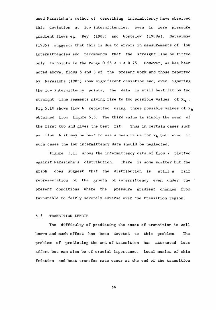
used Narasimha's method of describing intermittency have observed this deviation at low intermittencies, even in zero pressure gradient flows eg. Dey (1988) and Gostelow (1989a). Narasimha (1985) suggests that this is due to errors in measurements of low intermittencies and recommends that the straight line be fitted only to points in the range 0.25 < 7 < 0.75. However, as has been noted above, flows 5 and 6 of the present work and those reported by Narasimha (1985) show significant deviation and, even ignoring the low intermittency points, the data is still best fit by two straight line segments giving rise to two possible values of xt . Fig 5.10 shows flow 6 replotted using three possible values of obtained from figure 5.6. The third value is simply the mean of the first two and gives the best fit. Thus in certain cases such as flow 6 it may be best to use a mean value for xt but even in such cases the low intermittency data should be neglected.

Figure 5.11 shows the intermittency data of flow 7 plotted against Narasimha's distribution. There is some scatter but the graph does suggest that the distribution is still a fair representation of the growth of intermittency even under the present conditions where the pressure gradient changes from favourable to fairly severely adverse over the transition region.

5.3 TRANSITION LENGTHThe difficulty of predicting the onset of transition is well

known and much effort has been devoted to this problem. The problem of predicting the end of transition has attracted less effort but can also be of crucial importance. Local maxima of skin friction and heat transfer rate occur at the end of the transition

99

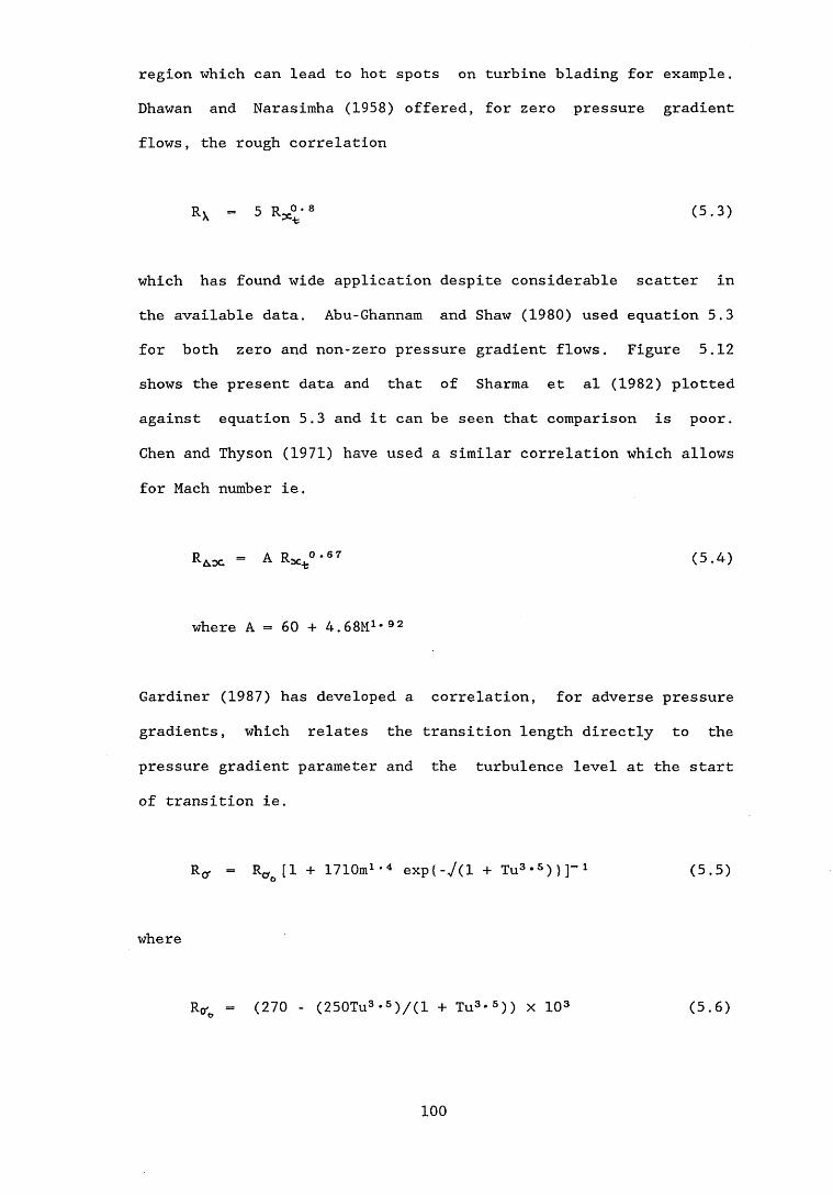
region which can lead to hot spots on turbine blading for example. Dhawan and Narasimha (1958) offered, for zero pressure gradientflows, the rough correlation

R\ = 5 Rx° * « (5.3)

which has found wide application despite considerable scatter in the available data. Abu-Ghannam and Shaw (1980) used equation 5.3 for both zero and non-zero pressure gradient flows. Figure 5.12 shows the present data and that of Sharma et al (1982) plotted against equation 5.3 and it can be seen that comparison is poor. Chen and Thyson (1971) have used a similar correlation which allows for Mach number ie.

where A = 60 + 4.68M1,92

Gardiner (1987) has developed a correlation, for adverse pressure gradients, which relates the transition length directly to the pressure gradient parameter and the turbulence level at the start of transition ie.

(5.4)

Ro. = Rtf [1 + 1710m1-4 exp{-7(1 + Tu3 *5)}]"*1w O (5.5)

where

Rtf - (270 - (250Tu3 *5)/(l + Tu3-5)) x 103 (5.6)

100

and Rtf = U o/vwhere o is the standard deviation of the Schubauer and Klebanoff (1955) distribution and can be related to A by

A = 1.37a (5.2)

Equation 5.5 was developed only for constant, mild adverse or zero pressure gradients ie. 0 < m < -0.04. Table 5.4 shows measured values of A alongside those predicted by equation 5.5. Bearing in mind the limitation of equation 5.5 the results are probably as good as could be expected.

More recently Narasimha (1985) has suggested that the transition length can be predicted from knowledge of the rate of spot production at the start of transition (see section 1.3). He suggested that the most appropriate non dimensional parameter is

N = noQZ/v (1.7)Using equation 1.6 the above equation can be rewritten as

N = 0.4120^ (5.7)X2u

or, alternativelyN = 0.412Re! (5.8)

Narasimha then suggests that in zero pressure gradient flows N has a "universal" value of 0.7xl0“3 for turbulence levels above about 1%. This value appears to rise for low values of freestreamturbulence. Using this universal value of N, if the start of transition can be located and 0 calculated, then A follows from

101

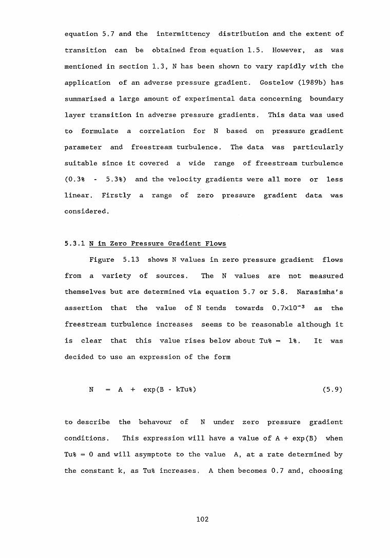
equation 5.7 and the intermittency distribution and the extent of transition can be obtained from equation 1.5. However, as was mentioned in section 1.3, N has been shown to vary rapidly with the application of an adverse pressure gradient. Gostelow (1989b) has summarised a large amount of experimental data concerning boundary layer transition in adverse pressure gradients. This data was used to formulate a correlation for N based on pressure gradient parameter and freestream turbulence. The data was particularly suitable since it covered a wide range of freestream turbulence (0.3% - 5.3%) and the velocity gradients were all more or less linear. Firstly a range of zero pressure gradient data was considered.

5.3.1 N in Zero Pressure Gradient FlowsFigure 5.13 shows N values in zero pressure gradient flows

from a variety of sources. The N values are not measuredthemselves but are determined via equation 5.7 or 5.8. Narasimha's assertion that the value of N tends towards 0.7xl0~3 as the freestream turbulence increases seems to be reasonable although it is clear that this value rises below about Tu% = 1 % . It was decided to use an expression of the form

N = A + exp(B - kTu%) (5.9)

to describe the behavour of N under zero pressure gradient conditions. This expression will have a value of A + exp(B) when Tu% = 0 and will asymptote to the value A, at a rate determined by

the constant k, as Tu% increases. A then becomes 0.7 and, choosing

102

a value of 2.5 for NxlO3 when Tu% = 0 leads equation 5.9 to become

Noxl03 = 0.7 + exp(0.588 - 3Tu) (5.10)

The zero turbulence value of 2.5 has little effect on the function and is perhaps irrelevant anyway as zero turbulence is an unobtainable ideal. Using a value of 3 for the constant k brings the function down to about 0.8 at Tu% = 1%. Equation 5.10 is shown along with the data of Gostelow (1989b) in figure 5.14 where the agreement is seen to be reasonable.

5.3.2 N in Adverse Pressure Gradient FlowsThe data of Gostelow (1989b) is shown in figure 5.15. It can

be seen that the non dimensional parameter N rises rapidly as the pressure gradient parameter becomes increasingly adverse but also that increased freestream turbulence has the effect of reducing N. This suggests that increasingly adverse pressure gradient dramatically increases the rate at which turbulent spots are produced, resulting in shorter transition lengths. It also suggests that increasing the freestream turbulence level reduces the rate of spot production leading to an increase in transition length which is in direct contrast with observations that increasing turbulence leads to a reduction in transition length eg.

Hall and Gibbings (1972) , Abu-Ghannam and Shaw (1980) and Fraser et al (1988).

The effect of adverse pressure gradient on the stability of laminar flow is well known. Stability theory has shown that, as the pressure gradient parameter becomes more negative, the critical

103

Reynolds number decreases and the maximum rate at which disturbances can be amplified increases. This has the effect of bringing the start of transition forward. It is possible that modification of the disturbance amplification rates is linked to the increase in spot production rate which leads to shorter transition lengths.

Increasing the freestream turbulence also has the effect of bringing the start of transition forward. In the flows of Gostelow

(1989b), and in the present flows, dU/dx is reasonably constant, at least in the area of interest. Thus, bringing the start of transition forward, by increasing the freestream turbulence, will result in the pressure gradient parameter, at the start of transition, becoming smaller in magnitude. This will result in a reduced spot formation rate which will lead to an increase in the transition length. This would appear to outweigh any effective reduction of the transition length due to the freestream turbulence. It therefore appears that, at least for Gostelow's data, the net effect of increasing the freestream turbulence is to increase the transition length. The data of Gostelow (1989b), and the present data, covers a wide range of adverse pressure gradients and freestream turbulence levels which are found in typical turbine blade flows but obvious care should be taken to avoid using the following correlation outwith this range.

Figure 5.15 suggests an exponential type of relationship between N and the pressure gradient parameter at the start of

transition, m , however log/linear plots failed to produce linear relationships. However, plotting ln(N) against freestream turbulence level for selected values of pressure gradient parameter

104

did reveal a near linear relationship as shown in figure 5.16. The mean slope of all the lines plotted in figure 5.16 was found to be about -0.45 thus

ln(Nxl03) = -0.45Tu + k (5.11)

where k is the value of ln(Nxl03) at the intercept where Tu = 0 and is obviously a function of the pressure gradient parameter. Figure 5.17 shows the values of k, obtained from fig 5.16, plotted against ln(m) which also produces a straight line relationship. A straight line fit gave a slope of 1.96 and an intercept of k=0.90. Since this was a purely empirical fit the slope was adjusted to 2 which gave an intercept of k=0.82 without significantly altering the fit of the straight line. Thus

which shows that the data of Gostelow (1989b) can be used to correlate N, fairly simply, to the freestream turbulence level at the leading edge and the pressure gradient parameter at the start of transition (xt determined by Narasimha's procedure). Equation 5.13 has one flaw in that it becomes zero when m becomes zero. This was overcome by simply adding the zero pressure gradient value of N obtained from equation 5.10, ie.

k = 2 ln(-mxlO2) + 0.82 (5.12)

When substituted into equation 5.11 this gives

N = 22.7m2exp(-0.45Tu) (5.13)

105

N N0 + 22.7m2exp(-0.45Tu) (5.14)

Both equations 5.13 and 5.14 are shown in figures 5.18a - d. It can be seen that the modified equation, 5.14, deviates from the original correlation, 5.13, as the turbulence level increases, particularly for low values of m. However this effect is exagerated by the logarithmic nature of the plot and it can be seen from figures 5.18a - d that equation 5.14 in fact gives a better correlation of the data. The data of Gostelow (1989b) is replotted, along with equation 5.14 for the appropriate turbulence

levels, on a linear scale in figures 5.19 and 5.20.Figure 5.21 shows the present data plotted against the

correlation, equation 5.14. Good agreement is obtained with flows 2, 3 and 4. Flows 5 and 6 are less satisfactory but they do at least follow the trend of decreasing N with increasing turbulence. Figure 5.22 shows the data of Gardiner (1987). This shows a fair amount of scatter but again the general trends are evident. It should be noted that the start of transition for this data is the 1% intermittency point rather than that obtained by Narasimha's procedure.

5.4 DETAILS OF TRANSITION

5.4.1 Integral ParametersThe behaviour of the main integral parameters through

transition are shown graphically in appendix 2. As well as the overall mean values, the values for the laminar and turbulent

106

components of the flow through the transition region are also shown. On the whole the mean parameters behave similarly to the results reported by Sharma et al (1982), particularly flow 6 which most closely resembled the flow studied by Sharma et al.

The behaviour of the momentum thickness Reynolds number, Rg , is shown in figures A2.1 to A2.6. The behaviour of the mean value is typical of a transitional boundary layer in that the rate of growth increases fairly suddenly after the start of transition. This is a result of the increasing influence of the turbulent component of the flow which has a much higher value of Rg from its inception. After the start of transition^Rg for the laminar component of the flow continues to grow at the same rate. However, towards the end of the transition region Rg for the laminar component shows a tendency to decrease.

Figures A2.7 to A2.12 show the behaviour of the shape factor Hu . In flow 6 the flow remains attached but the mean shape factor reaches a value of about 3 at the start of transition which is indicative of the adverse pressure gradient. The shape factor of the turbulent component has a much lower value, typical of a fully developed turbulent boundary layer, from the start of transition. This causes the mean value to drop as the proportion of turbulent flow increases. H ia of the laminar flow remains high before dropping off rapidly towards the end of transition. This may be due to the stabilising effect of the passage of turbulent spots first reported by Schubauer and Klebanoff (1955). It can be seen from the velocity profiles (see appendix 3) that towards the end of transition the laminar profiles become fuller indicating increased stability of the remaining laminar flow. Flows 1 to 5 follow a

107

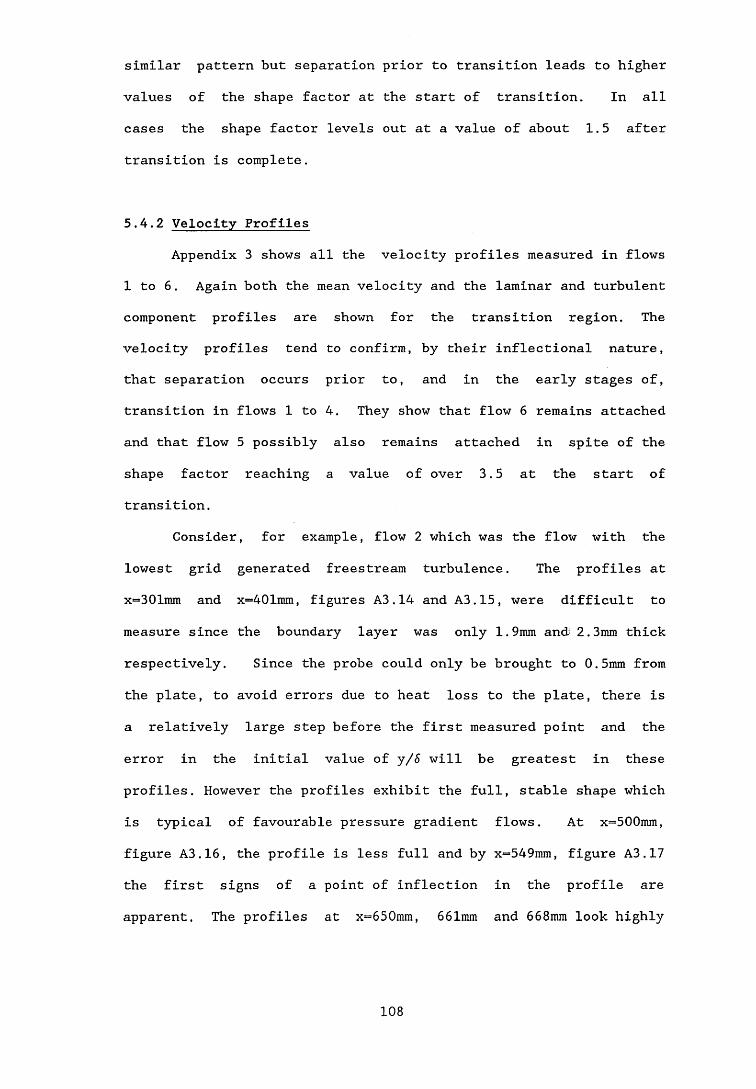
similar pattern but separation prior to transition leads to higher values of the shape factor at the start of transition. In all cases the shape factor levels out at a value of about 1.5 after transition is complete.

5.4.2 Velocity ProfilesAppendix 3 shows all the velocity profiles measured in flows

1 to 6 . Again both the mean velocity and the laminar and turbulent component profiles are shown for the transition region. The velocity profiles tend to confirm, by their inflectional nature, that separation occurs prior to, and in the early stages of, transition in flows 1 to 4. They show that flow 6 remains attached and that flow 5 possibly also remains attached in spite of the shape factor reaching a value of over 3.5 at the start of transition.

Consider, for example, flow 2 which was the flow with the lowest grid generated freestream turbulence. The profiles at x=301mm and x=401mm, figures A3.14 and A3.15, were difficult to measure since the boundary layer was only 1.9mm and 2.3mm thick respectively. Since the probe could only be brought to 0.5mm from the plate, to avoid errors due to heat loss to the plate, there is a relatively large step before the first measured point and the error in the initial value of y/S will be greatest in these profiles. However the profiles exhibit the full, stable shape which is typical of favourable pressure gradient flows. At x=500mm, figure A3.16, the profile is less full and by x=549mm, figure A3.17 the first signs of a point of inflection in the profile are apparent. The profiles at x=650mm, 661mm and 668mm look highly

108

inflectional and, with shape factors of almost 4, indicate that the flow has separated.

At the next measurement station, x=680mm, figure A3.22, transition is underway and the near wall intermittency has a value of 0.12. The bulk of the flow, which is laminar, still appears to be separated with a shape factor of about 3.5 and a velocity profile which is highly inflectional. The turbulent component velocity profile is typical of a fully turbulent boundary layer in a severe adverse pressure gradient, however it appears to be attached. Thus it would seem that developing turbulent spots can remain attached in a separating laminar flow from an early stage in the transition process. This would lead to the observation of intermittent laminar separation in the transition region. A similar pattern is observed at the next point, x=691mm, figure A3.23, but because of the increased proportion of turbulent flow, the mean velocity profile is less severely inflectional than the laminar component. At x=695mm, figure A3.24, the laminar profile is still inflectional and has a shape factor of 3.2, indicating that it may still be separated, but because the intermittency is almost 0.5, the mean velocity profile no longer has a point of inflection. As the turbulence becomes the dominant flow regime the laminar component profiles become more stable as can be seen in figures A3.25 to A3.28. The turbulent boundary layer is much more resistant to adverse pressure gradients than the laminar boundary layer as is illustrated by the profiles in figures A3.29 to A3.32. These profiles show some effect of the adverse pressure gradient but are obviously in no imminent danger of separating.

As the turbulence level is increased the start of transition

109

is brought forward. This is shown in figure 5.23 which also includes data from Sharma et al (1982). Since the end of transition is not affected as much, the transition length increases as shown in figure 5.24. Bringing the start of transition forward ultimately means that the start of transition occurs before the point of laminar separation and the growth of the turbulent spots can prevent separation as in flow 6 and possibly flow 5. In both flows 5 and 6 the mean profiles show slight inflections prior to the start of transition. After the start of transition the inflection becomes more marked in the mean and laminar profiles, see figures A3.68, A3.69 and A3.86. Again, however, as the turbulence occupies increasingly more of the flow the laminar flow becomes stabilised while an attached turbulent boundary layer eventually emerges.

5.4.3 Flow 7The velocity distribution of flow 7 is shown in figure A2.13

in appendix 2 and the integral parameters are shown in figures A2.14 and A2.15. The velocity profiles are shown in figures A3.103 to A3.113 in appendix 3. The momentum thickness Reynolds number exhibits similar behaviour through transition to flows 1 to 6 . The shape factor also behaves similarly to flows 1 to 6 although the shape factor for the laminar component profile rises more sharply than the mean value after the pressure gradient changes from favourable to adverse. The shape factor for the turbulent component profile seems to be unaffected by the change in pressure gradient and the remaining laminar flow becomes stabilised by the increasing proportion of turbulent flow. The velocity profiles show

110

that the laminar component profile becomes slightly inflectional between x=750, figure A3.110, and x=780, figure A3.Ill, but this does not lead to laminar separation before the boundary layer becomes fully turbulent.

Ill

DATA SUMMARIES

FLOW Tu Xa(mm) xt (mm) 0-t (mm) Ret A (mm) RA -m1 1.00 663 669 0.56 525 23 21563 0.1292 1.06 670 673 0.60 560 17 15867 0.1483 1.08 669 679 0.58 530 16 14621 0.1384 1.12 658 663 0.56 510 17 15482 0.1295 1.53 610 634 0.57 525 30 27632 0.1336 2.06 564 592 0.53 500 51 48113 0.115

Table 5,

FLOW

, 1 Summary of

measuredRftt

transition data

Abu-Ghannam Tu (L.E.)

and Shaw Tu(x-fc)

1 525 381 5072 560 381 5293 530 368 5114 510 359 5075 525 296 4346 500 245 397

Table 5.2 Comparison of measured and predicted values of R q^

xt (mm) 0t(mm) A(mm) m

6250.34680.027

Table 5.3 Data for flow 7

FLOW A(meas) A(eqn 5.5)1 23 112 17 83 16 114 17 115 30 116 51 13

Table 5.4 Measured and calculated values

112

intermittency distributionflow 1

1/2.

D intermittency

figure 5.1

intermittency distribution flow 2

1/ 2 .Hn(1-V)i

D intermittency

figure 5.2

113

intermittency distributionflow 3

1/2.

0 intermittency

figure 5.3

intermittency distribution flow 4

1/2I-in(l-Y)]

a intermittency

figure 5.4

114

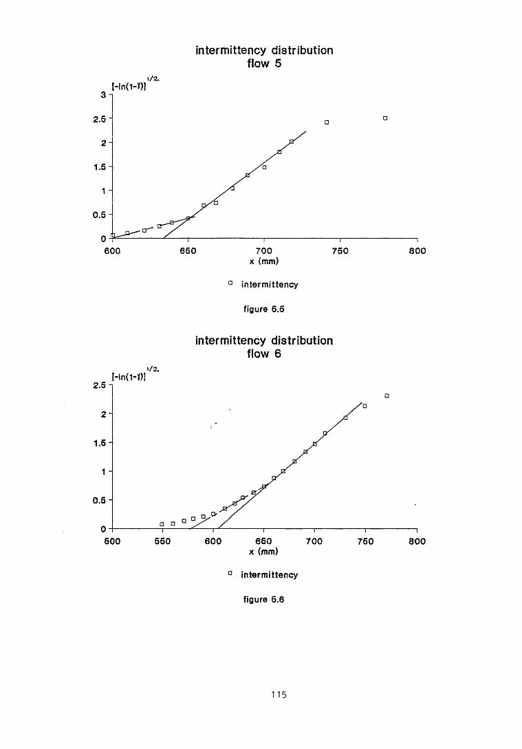
intermittency distributionflow 5

Hn(1-T)J1/2.

a intermittency

figure 5.5

intermittency distribution flow 6

»/2.Hn(1-lf)J

a intermittency

figure 5.6

115

velocity/intermittency distributionflow 7

D velocity * gamma

figure 5.7a

intermittency distribution flow 7

0 .5 -

0 —300

° intermittency

figure 5.7b

400 500 600 x (mm)

700 800

»/z.Hn(1-y)]

2 .5 1

2-

1.5*

D

--1900

116

117

*

1 1

0.8 -

0.6 -

0.4 -

0.2 -

0 —

-3

normalised intermittency distributions(Schubauer and Klebanoff method)

..O.ft & v DV

V

d 7 ° <Y 0

o DVV

o

VSX

27

O V

□ 0

V ° X V A 0°

-2 -1 0 1 3

3 flow 1

1 flow 4

^ flow 2

° flow 5

A f low 3

v flow 6

figure 5.8

X

normalised intermittency distributions(Narasimha’s method)

flow 1 0 flow 2 A flow 3

flow 4 o flow 5 v flow 6

figure 5.9

normalised intermittency distributions(Narasimha’s method) - flow 6

a xt * 606 0 xt • 577 A xt ■ 592 ----- 1 -ex p (-0 .4 1 2 f )

figure 5.10

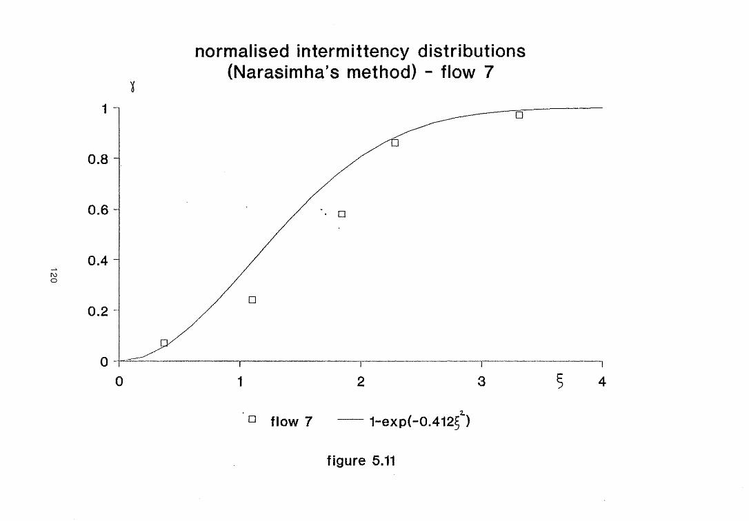
120

normalised intermittency distributions(Narasimha’s method) - flow 7

I

figure 5.11

transition length correlation of Dhawan and Narasimha

-3

R \ * 5 R ^ D flows 1 to 6 o flow 7 A Sharma

figure 5.12

122

spot formation rate in zero pressure gradient

N*103

D SS 0 As A GR 2 BW O p V G + GB

figure 5.13

N in zero pressure gradients

N*103

eqn 5.10 D Gostelow(1989b)

figure 5.14

- 0.10 - 0.08 - 0.06 - 0.04 - 0.02 0.00 0.02

Lambda Theta t

figure 5.15 data of Gostelow (1989b)

N against Tu% at constant pressure gradient parameter, m

N*10 100 q

VV

o o VX X o

A XA

0A

0 0

□□

1 =

0.1 H----------------- 1------------------r

0 1 2

D m ■ 0.01 0 mz m ■ 0.04 O m

VO

X 0

AX V

oA

X

0 0 A

□□

0

3 4 5 6Tu%

0.02 A m ■ 0 .03

0.05 V m ■ 0 .06

figure 5.16

"k" against pressure gradient parameter

k5 i

□

4 -□

□

3 - □

2 -□

1 -

0 i-------------------- 1----------- !-------- !------ 1-----i---- 1--- 1--- 1-- 1

0.01 0.1m

° k

figure 5.17

126

equations 6.13 and 6.14 m - 0.01

N*101 0 0 3

10

0.1 — 1—

3Tu%

eqn 6.13 eqn 6.14 0 Goatelow (1989b)

figure 6.18a

po-on*io

equations 6.13 and 6.14 m - 0.04

3Tu%

eqn 6.13 ..... eqn 6.14 ° Goatelow (1989b)

figure 6.18c

equations 6.13 and 6.14 m • 0.02

N‘10

----- eqn 6.13 eqn 6.14 Q Goatelow (1989b)

figure 6.18b

equations 6.13 and 5.14 m •* 0.06

N*10

----- eqn 6.13 ...... eqn 6.14 D Goatelow (1988b)

figure 6.18d

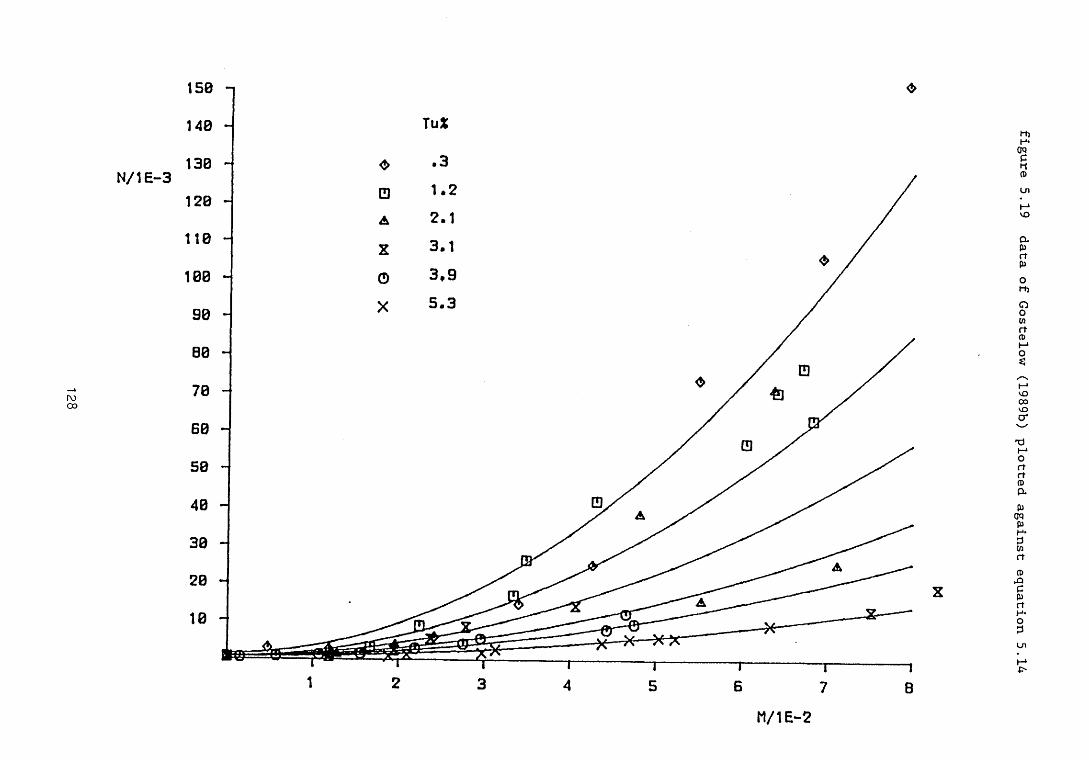
figure 5.19 data of Gostelow (1989b) plotted against equation 5.14

128

M/ 1 E- 2

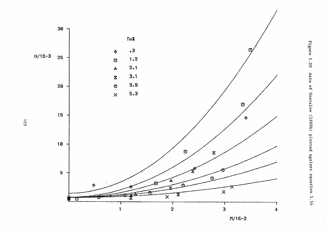
Tu% figure 5.20 data of Gostelow (1989b) plotted against equation 5.14

129

2-3l/U

F lo w figure 5.21 present data plotted against equation 5.14

130

M / 1 E - 2

N /1 E - 3

figure 5.22 data of Gardiner (1987) plotted against equation 5.14

inin

••

IN1!

IIii

1!a

aa

3h*

1—

131

M/ 1 E- 2

x against Tu%

x (mm) 700 i

o>A

600 -z

o

5 0 0 - v

400 J-------------------- r0 0.5 1

Tu%1.5 2 2.5

+ flow 1 ° flow 2 0 flow 3 A flow 42 flow 5 ° flow 6 V Sharma ot al (1982)

figure 5.23

X against Tu%

(mm)

+ flow 1 a flow 2 0 flow 3 A flow 42 flow 6 ° flow 6 v Sharma et al (1982)

figure 5.24

1 3 2

CHAPTER 6

BOUNDARY LAYER PREDICTION

The so called differential methods of solving the boundary layer equations, which solve the basic partial differential equations numerically, have been developed over the last thirty years. These methods have largely been programmed to run on mainframe or mini computers because of the considerable number of calculations which are required for even fairly simple analyses. However modern microcomputers are having an impact in numbercrunching applications as well as other areas, such as data acquisition. The newer microcomputers have sufficient memory capacity to allow realistic problems to be defined and faster processing speeds allow solutions to be obtained in acceptable times. Thus it is now practical to use differential methods for routine design calculations in many cases. A proven method, which is applicable to laminar and turbulent boundary layers, is that of Cebeci and Smith (1974). This method uses the so called box method due to Keller (1970). A Fortran program for this method is given by Cebeci and Bradshaw (1977) and this was adapted to run, incompiled BASIC, on the Amstrad PC1640 microcomputer. The nextsection gives a very brief description of the method.

6.1 THE CEBECI-SMITH METHODThe x-momentum equation can be written for two dimensional,

laminar or turbulent boundary layers asu3u + vdu = U dU + 1 3_ I" f i d u + p edu 1 (6.1)6x dy dx P dy l dy dy J

where e is the eddy viscosity, which is zero in laminar flow. Equation 6.1 is transformed using the Falkner-Skan transformation. The advantage gained is that the boundary layer thickness in

134

transformed coordinates remains almost constant in laminar flow and the rate of growth is much reduced in turbulent flow. This means that a relatively simple grid representation can be employed.

The Falkner-Skan transformation is defined by

r1 - f u j ° ' 5 V ( 6 . 2 )

and a dimensionless stream function, f (x, r/), is introducedV>(x,y) - (U i/x)°‘ sf (x, tj)

After some manipulation equation 6 .1 becomes(bf' ') ' + fm+ll ff' ' + m[l -(f')2] = xff'Sfl - f"<yf|[ 2 J [ 5 x 3xJ

(6.3)

(6.4)

where b = (1 + e+), with e+ = e/i/ and m = x 3U and the prime,U dx

denotes differentiation w. r . t. rjEquation 6.4 is then written as a system of first order

P.D.E.s ie.f' = u (6.5a)u' = v (6.5b)(bv)' + fm+llfv + m(l-u2) = xfudu - vdfl (6.5c)[ 2 J [ a x axjEquations 6.5 are then written in finite difference form

using "centred difference" derivatives. An arbitrary grid is assumed in the formulation of the finite difference equations which allows varying step sizes to be used when solving particular problems. The equations are implicit and non linear and are solved using Newton's method. This is carried out using the block elimination method as discussed by Keller (1974) and described in detail by Cebeci and Bradshaw (1977). For laminar boundary layers

135

the eddy viscosity, e, is zero and the solution of equations 6.5 becomes a purely mathematical problem. Great accuracy can be achieved by using suitable grids and a number of test cases are examined in chapter 8 of Cebeci and Smith (1974).

Predicting turbulent boundary layers is considerably more difficult than predicting laminar boundary layers. Turbulent boundary layers tend to be much thicker than laminar boundary layers yet the velocity gradient, 3u/3y, can be greater at the wall. This requires that short steps be taken, in the y direction, close to the wall which would lead to large numbers of points if a constant grid was used. However, because the Cebeci-Smith method allows for an arbitrary grid it is advantageous to use a geometric progression in the y (or rj in the transformed equations) direction. This allows fine resolution to be used close to the wall but the spacing becomes larger away from the wall giving an economical number of grid points across the boundary layer. Similarly, varying resolution can be employed in the x direction eg. using finer resolution near separation.

The turbulent boundary layer equations are further complicated by the existance of fluctuation terms, the so called Reynolds stresses. The Reynolds stress terms cannot be obtained analytically and must be modelled. The Cebeci-Smith method uses an eddy viscosity method which relates the Reynolds stresses to the mean flow ie.

-pu'v' = pedu (6 .6 )ay

The turbulent boundary layer is treated as a composite layer with inner and outer regions and separate expressions are given for the

136

eddy viscosity in each region. In the inner region the eddy viscosity is defined by a "mixing length" type equation

L2 3u 7 , 0 < y < yc (6.7)

The mixing length, L, is given by an extended version of Van Driest's model, see Cebeci and Smith (1974). In the transition region the eddy viscosity is weighted by the intermittency and thus affects only the first term in equation 6.4. This is only an approximation since equation 6.4 is non linear but it has been widely used and found to be reliable. A more correct approach would be to solve equation 6.4 separately for the laminar and turbulent components of the flow, and weight the solutions using the intermittency. This is effectively the same technique as that employed by Fraser and Milne (1986) and others for integral methods in that the transitional boundary layer is considered to be a weighted combination of laminar and fully turbulent boundary layers. In the outer region the eddy viscosity is defined by

where a is taken as a universal constant, a = 0.0168. yc isdefined as the point where e-t = eo.

Because of the difficulty of predicting the location of the start of transition this is normally treated as a direct input. The Cebeci-Smith method uses the method of Chen and Thyson (1971) to calculate the length of the transition region and the intermittency distribution. This method has been found to fare rather poorly when predicting turbine blade flows, usually predicting transition lengths which are far too long. This method is compared, in the

( 6 . 8 )

o

137

next section, with an alternative based on the correlation described in the previous chapter. Equations 5.10 and 5.14 are used to determine the value of N at the start of transition using the inlet turbulence level and the local pressure gradient parameter. The transition length, in terms of A, is then obtained from equation 5.7 or 5.8 and the intermittency distribution is given by equation 1.5.

6.2 PERFORMANCE OF THE C-S METHODThe Cebeci-Smith method has been shown to be reliable for a

wide range of laminar and turbulent flows. See, for example, Cebeci and Bradshaw (1977) . The method is now compared with some of the present experimental data ie. flow 6 . For the present velocity distribution the C-S method predicts laminar separation at about x = 590mm. This ties up with the observation that flows 1 to 5 all exhibit laminar separations prior to the start of transition since the start of transition is later than x = 590mm in all cases (whether defined as xs or xt) . Although x - is 592mm in flow 6 , xs is 564mm, therefore the flow will not be completely laminar at x = 590mm. After separation is encountered the C-S method fails since convergence can no longer be attained. Only flow 6 remains attached throughout and this is the only flow that can be calculated completely.

Flow 6 was calculated twice, using both the Chen and Thyson (1971) method and the procedure described in chapter 5 (equation 5.14) for the transition region. The results are shown in figures 6.1, 6.2 and 6.3. Figure 6.1 shows the intermittency distribution. It can be seen that the Chen and Thyson method predicts a much

138

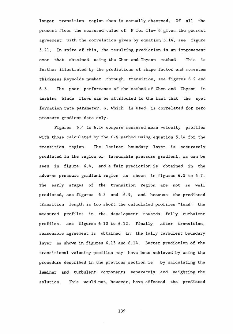
longer transition region than is actually observed. Of all the present flows the measured value of N for flow 6 gives the poorest agreement with the correlation given by equation 5.14, see figure 5.21. In spite of this, the resulting prediction is an improvement over that obtained using the Chen and Thyson method. This is further illustrated by the predictions of shape factor and momentum thickness Reynolds number through transition, see figures 6.2 and 6.3. The poor performance of the method of Chen and Thyson in turbine blade flows can be attributed to the fact that the spot formation rate parameter, G, which is used, is correlated for zero pressure gradient data only.

Figures 6.4 to 6.14 compare measured mean velocity profiles with those calculated by the C-S method using equation 5.14 for the transition region. The laminar boundary layer is accurately predicted in the region of favourable pressure gradient, as can be seen in figure 6.4, and a fair prediction is obtained in the adverse pressure gradient region as shown in figures 6.5 to 6.7.The early stages of the transition region are not so wellpredicted, see figures 00 and 6.9, and because the predictedtransition length is too short the calculated profiles "lead" the measured profiles in the development towards fully turbulent profiles, see figures 6.10 to 6.12. Finally, after transition, reasonable agreement is obtained in the fully turbulent boundary layer as shown in figures 6.13 and 6.14. Better prediction of the transitional velocity profiles may have been achieved by using the procedure described in the previous section ie. by calculating the laminar and turbulent components separately and weighting the solution. This would not, however, have affected the predicted

139

transition length or intermittency distribution. Future work may show whether the extra computational effort which would be involved is justified by improved accuracy.

The Cebeci-Smith boundary layer calculation method is commonly used to predict flows, such as those over turbine blades, which involve transition in adverse pressure gradients. By using equation 5.14 in conjunction with equations 5.7 and 1.5, which takes account of the effects of adverse pressure gradient, improved prediction of the transition region in such flows is achieved. It is possible to extend the C-S method to calculate separating and reattaching flows by using the so called inverse boundary layer approach, see for example Cebeci et al (1979) . This approach requires, however, that the displacement thickness be specified in advance. Cebeci (1989) used the C-S method interactively with an inviscid method to calculate flows over aerofoils which included separation bubbles. Such a procedure should be applicable to flows 1 to 5 of the present work. The improvement of equation 5.14 over the Chen and Thyson model might be expected to be even more marked since the measured values of N for flows 1 to 5 were in better agreement with equation 5.14 than flow 6 .

140

C -S Calculation Method intermittency

Gamma1 .2 -i

1 -

0 .8 -

0 .6 -

0 .4 -

0 .2 -

0 ------0

Q Q 03

I /

□□

a

-i---------- ¥---- &0.2 0.4 0.6 0.8

x (m>

Ch-Thy ----- N method ° expt data

figure 6.1 C-S prediction, flow 6

C -S Calculation Method shape factor

H3.5 -i

3 -

2.5

2 -

1.5- CT '

1 - 0 .5 -

0 ---------- 1---------- 1-----------1---------- 1—0 0.2 0.4 0.6 0.8

x (m)

Ch-Thy ----- N method ° expt data

figure S.2 O—S prediction, flow 6

i1

n1

141

C -S Calculation Method momentum thickness Re

Re1400 -

1200- 1000

8 0 0 -

6 0 0 -

4 0 0 -

200 - 0 — i—

0.2 0.4 0.6x (m)

0.8

Ch-Thy N method D expt data

figure 6.3 C-S prediction, flow 6

1 4 2

y/delta

i'i

\o

! I

J

t

iitII*_i

figure 6.4 velocity profile prediction with expt data

143

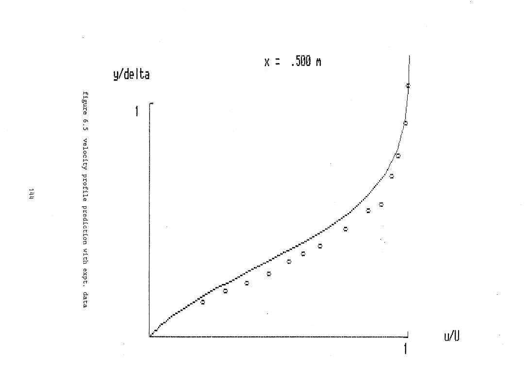
y/delta w■J~g

a

M

oC=DLT5•

! IX

figure 6.5 velocity profile prediction with expt. data

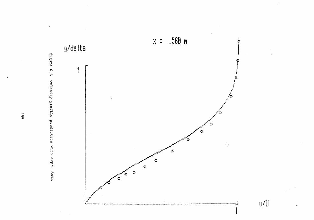
y/delta

H

=- * a

'« O

CSSCj=sm

\uK 31

I !X

V ,:i*»_\ n*. r»■s

t>•H

figure 6.6 velocity profile prediction with expt. data

145

y/delta

--4J

f s

~ u~-5 C

O

LT>! !

I

O

figure 6.7 velocity profile prediction with expt. data

146

y/delta

i

figure 6.8 velocity profile prediction with expt. data

147

y/d elta

r■*+

—Jj

—-O

■-is

h

C*-4C

O«

I IX

I

figure 6.9 velocity profile prediction with expt. data

148

y/d e lta

——-£s-_-H

..

■J

CD

■*

CO11

os

si

ri

O

iiu

11

i_«O

3 i

*. I

*. 3I

i i

I I

yi!'i31

figure 6.10 velocity profile prediction with expt. data

149

y/delta

o

¥l.

ijo

o

CjZsC£=5I 1X

osi*

riOo1

oo

L

figure 6.11 velocity profile prediction with expt. data

150

y/delta

%■-O

-------------34.

rt..f

t..

ft Vo

oSIS3UCOCO

•

I iX

II

81o18M X

° \. i

II i

L

figure 6.12 velocity profile prediction with expt. data

151

y/delta

O'--..

CDCDI IX

oo \ii

oSIIIIt

_ i

1 a *O V*hiL*,lI

l

figure 6.13 velocity profile prediction with expt. data

152

y/deIta

CD

COI !>C

rs--_■a.

Si

i'i3 I

o

\

S.a■«oIIni - «III

L

figure 6.14velocity profile

prediction with exptdata

153

CONCLUSIONS

1. The existing boundary layer wind tunnel has been modified to give a velocity distribution typical of a forward loaded turbine blade ("squared-off" design) over the test plate

2. A data acquisition and control system based on the AMSTRAD PC1640HD20 microcomputer was developed. By utilising assembly language subroutines, very fast sampling rates could be achieved which allowed a detailed digital representation of the raw signal to be captured. The large RAM capacity of the AMSTRAD PC1640 ensured that samples of sufficient length could be stored. The presence of a 20MByte hard disk allowed many such samples to be gathered and stored before subsequent processing at a later, more convenient, time.

3. Software techniques were developed for the calculation of mean flow variables, such as mean velocity and RMS, thus reducing the requirement for external instrumentation. Assembly language subroutines were again necessary to process the large quantities of data involved within acceptable timescales.

4. An algorithm was developed to discriminate between laminar and turbulent flow. This was used to conditionally sample the signal in the transition region and hence provide mean laminar and turbulent velocity profiles in the transition region. It also provided a measurement of the intermittency.

5. Simple intermittency weighting of laminar and turbulent components to give a transitional parameter is not strictly

155

applicable to the component profiles measured during the present work. A corresponding expression for displacement thickness which takes into account the variation of intermittency in the y direction was developed (equation 4.19). This was shown to be more accurate when applied to the current data.

6. Boundary layer profiles were measured under the imposed velocity distribution at various levels of freestream turbulence.

7. Two methods of defining the start of transition were compared, ie. the 1% intermittency point, xs , and the method of Narasimha (1985) which gives xt. In all cases xs was found to occur earlier than x^. Conditions at xt were found to give better results when correlating the spot formation rate parameter, N, (see no. 10).

8. The concept of statistical similarity of transition regions was observed to remain intact for severe adverse pressure gradients, including cases where separation bubbles were present during the early stages of transition.

9. The mean intermittency distributions of Schubauer and Klebanoff (1955) and Dhawan and Narasimha (1958) were compared for the present data. The S-K distribution appears to give the better fit but is likely to be less practical in a calculation scheme since it requires that the 50% intermittency point be known. The D-N distribution depends on x^ which can be difficult to locate

accurately.

156

10. A correlation for the spot formation rate parameter, N, has been developed, equation 5.14, which accounts for the combined effects of freestream turbulence level and pressure gradient (adverse pressure gradients only).

11. Conditionally sampled velocity profiles indicate that intermittently separated laminar flow and attached turbulent flow can occur in the early part of the transition region.

12. The differential boundary layer calculation method of Cebeci and Smith (1974) appears to be better equipped to calculate turbine blade flows as a result of the inclusion of the new correlation.

157

SUGGESTIONS FOR FUTURE WORK

The transition length obtained from the correlation, equation 5.14, is based on the premise that the most important governing factor is the rate at which spots are formed at the start of transition. Possible variations of the spot propagation characteristics, such as the spread angle, are not explicitly considered. Very little experimental data exist regarding the influence of pressure gradient on the propagation characteristics of turbulent spots and more such data would be helpful in providing improved models of the transition region.

The present work has shown that a high level of sophistication in data acquisition and reduction can be achieved at fairly low cost by using a 16-bit microcomputer. Similar systems could be used to carry out detailed investigations of spot propagation characteristics under the influence of various pressure gradients. Indeed, 16-bit microcomputer based data acquisition and control systems could be used in a wide variety of applications which previously required access to mainframe and mini computers.

159

REFERENCES

Abu-Ghannam B.J. & Shaw R. - "Natural Transition of Boundary Layers-The Effects of Turbulence, Pressure Gradient and Flow History" Jour Mech. Eng. Science, Vol. 22 1980

Arnal D., Juillen J.C. & Michel R.

- "Experimental Analysis and Computation of the Onset and Development of the Boundary Layer Transition". AGARD conf. Proc No. 224, Laminar-Turbulent Transition, paper no 13, 1977 (English translation NASA TM 75325

Birch N.T. - "Navier-Stokes Predictions ofTransition, Loss and Heat Transfer in a Turbine Cascade". ASME-GT-22 1987a

Birch N.T. - "Comparison Between Numerical Solutions and Measurements for a High-Speed Turbine Blade". C268/87 I Mech E 1987b

Blair M.F., Bailey D.A. & Schiinker R.H.

- "Development of a Large-Scale Wind Tunnel for the Simulation of Turbomachinery Airfoil Boundary Layers". ASME J. of Eng. for Power, Vol 103, 1981

Blair M.F. & Werle M.J. - "The Influence of Freestream Turbulence on the Zero Pressure Gradient Fully Turbulent Boundary Layer". UTRC Report R80-914388-12, 1980

Bluechip Technology - ACM-44 Technical manual, document reference acmu 1011, 1988

Cantwell B., Coles D. & Dimotakis P.

- "Structure and Entrainment in the Plane of Symmetry of a Turbulent Spot". J. Fluid Mech., Vol 87, Part 4, 1978

Cebeci T. - "Essential Ingredients of a Method for Low Reynolds-Number Airfoils". AIAA Jour., Vol 27, No 12, 1989

Cebeci T. & Bradshaw P. - "Momentum Transfer in Boundary Layers". McGraw-Hill, 1977

Cebeci T., Keller H.B. & Williams P.G.

- "Separating Boundary layer Flow Calculations". Jour. Comp. Phys., Vol. 31, 1979

161

Cebeci T. & Smith A.M.O. - "Analysis of Turbulent Boundary Layers". Academic Press, New York 1974

Cedar R.D. & Stow P. - "A Compatible Mixed Design and Analysis Finite Element Method for the Design of Turbomachinery Blades". Int. J. for Num. Methods in Fluids. Vol. 5, 331-345 1985

Chen K.K & Thyson N.A. - "Extension of Emmons' Spot Theory to Flows on Blunt Bodies". AIAA Jour. Vol. 9, 1971

Coles D.E. - "The Law of the Wake in the Turbulent Boundary Layer". J. Fluid Mech. Vol 1, 1956

Coles D.E. - "The Young Persons Guide to the Data". Proc. Computation of Turbulent Boundary Layers. Vol II pp 1 - 53, Stanford Conf. 1968

Coles D.E. & Hirst E.A. - "Computation of Turbulent Boundary Layers". AFOSR-IFP-Stanford Conf. Vol II. 1968

Corrsin S. & Kistler A.L. - "Freestream Boundaries of Turbulent Flows". NACA Report 1244, 1955

Dey J. - "An Integral Method for the Calculation of 2-D Transitional Boundary Layers". Ph.D. Thesis, Indian Institute of Science, 1988

Dhawan S. & Narasimha R. - "Some Properties of Boundary Layer Flow During The Transition From Laminar to Turbulent Motion".Jour. Fluid Mech., Vol. 3, 1958

Dzung L.S. & Seippel C. - "Aerodynamic Aspests of Blading Research" Flow Research on Blading. Elsevier Publishing Company, 1970

Emmons H.W. - "The Laminar-Turbulent Transition in a Boundary Layer - Part 1". Jour. Aero. Sci. Vol. 18, 1951

Fraser C.J. - "Boundary Layer Development From Transition Provoking Devices". PhD Thesis, Dundee College of Technology, 1979

162

Fraser C.J., Gardiner I.D. & Milne J .S.

- "A Comparison of Two Integral Techniques for the Prediction of Transitional Boundary Layer Flow”. Conf. on Numerical Methods in Laminar and Turbulent Flow, Montreal, 1987

Fraser C.J., Graham D. & Milne J.S.

- "Digital Processing of Hot Wire Anemometer Signals in Intermittently Turbulent Flows" Flow Meas. Instrum., Vol 1, 1990

Fraser C.J. & Milne J.S. - "Integral Calculations ofTransitional Boundary Layers". Proc. I Mech E, Part C 200, 1986

Fraser C.J., Milne J.S. & Gardiner I.D.

- "The Effect of Pressure Gradient and Freestream Turbulence Intensity on the Length of Transitional Boundary Layers". Proc Instn Mech Engrs, Vol 202 No C3, 1988

Fraser C.J., Milne J.S. & Graham D.

- "Fast Data Acquisition and Digital Signal Processing in Studies of Turbulent Flow". 4th Joint Int. Conf. on Mech. Eng. 6c Tech. , Zagazig Univ. Cairo, 1989

Gad-el-Hak M., Blackwelder R.F. & Riley J.J.

- "On the Growth of Turbulent Regions in Laminar Boundary Layers". J . Fluid Mech. Vol 110, 1981

Gardiner I.D. - "Transition in Boundary LayerFlows". PhD thesis, Dundee College of Technology, 1987

Gardner W.B. - "Energy Efficient Engine Low Pressure Turbine Boundary Layer Program Technology Report". NASA CR-165338 (PWA-5594-141)

Gostelow J .P. - "Adverse Pressure Gradient Effects on Boundary Layer Transition in a Turbulent Free Stream". 9th ISABE, Athens, 1989a

Gostelow J .P. - personal communication, 1989bGostelow J.P. 6s Blunden A.R. - "Investigations of Boundary Layer

Transition in an Adverse Pressure Gradient". ASME Paper No 88-GT-298, 1988

163

Graham D., Fraser C.J. & Milne J .S

- "Digital Measurement inIntermittently Turbulent Flows". AMSE conf Signals & Systems, Brighton, 1989

Hall D.J. & Gibbings J.C. - "Influence of Freestream Turbulence and Pressure Gradient Upon Boundary Layer Transition". J. Mech Eng Sci, Vol. 14, No 2, 1972

Horton H.P. - "A Semi-empirical Theory for the Growth and Bursting of Laminar Separation Bubbles". 1967

Kaplan R.E. & Laufer J. - "The Intermittently Turbulent Region of the Boundary Layer". Proc. 12th Int. Cong, of Appl. Mech. Springer-Verlag, 1969

Keller H.B. - "A New Difference Scheme for Parabolic Problems". Numerical Solutions of Partial Differential Equations, Vol. 2, Academic Press, 1970

Keller H.B. - "Accurate Difference Methods for Nonlinear Two-Point Boundary Value Problems". SIAM J. Numer. Anal. Vol 11, 1974

Klebanoff P.S. - "Characteristics of turbulence in a Boundary Layer With Zero Pressure Gradient". NACA Tech note 3178, 1955

Kline S.J., Cockrell D.J., Morkovin M.V. & Sovran G.

- "Computation of Turbulent Boundary Layers". AFOSR-IFP-Stanford Conf. Vol I. 1968

Kovasznay L.S.G., Kibens V. 6c Blackwelder R.F.

- "Large-Scale Motion in theIntermittent Region of a Turbulent Boundary Layer". J. Fluid Mech. Vol 41, 1970

Liu Y.C. 6c Gibson G.A. - "Microprocessor-Based Systems: The 8086/8088 Family". Prentice-Hall, 1984

Ludwieg H. 6c Tillman W. - "Investigation of the Wall Shearing Stress in Turbulent Boundary Layers". NACA Tech memo 1285, 1950

164

McCormick M.E.McCormick M.E.

McDonald H. & Fish R.W.

- "An Analysis of the Formation of Turbulent Patches in the Transition Boundary Layer". Trans. ASME, J. App. Mech., Vol 35, 1968

- "Practical Calculations of Transitional Boundary Layers". Int Jour Heat & Mass Transfer Vol. 16, No. 9, 1973

Mur1is J . - "The Structure of a Turbulent Boundary Layer at Low Reynolds Number". Ph.D. thesis, Imperial College, London, 1975

Murlis J., Tsai H.M. & Bradshaw P.

- "The Structure of Turbulent Boundary Layers at Low Reynolds Numbers". J. Fluid Mech. Vol 122, 1982

Narasimha R. - "On the Distribution OfIntermittency in the Transition Region of a Boundary Layer". J. Aero. Sci. Vol 24, 1957

Narasimha R. - "The Laminar-Turbulent Transition zone in the Boundary Layer". Prog. Aerospace Sci. Vol. 22, 1985

Orr W.M.F. - "The Stability or Instability of the Steady Motions of a Perfect Fluid and of a Viscous Liquid". Proc. Royal Irish Acad. Vol. 27 1907

Pohlhausen K. - "Zur Naherungsweisen Integration der Differentialgleichung der Laminaren Reibungsschicht". Zeit fur Ang. Math. 6s Mech. , Vol 1. 1921

Rector R. & Alexy G. - "The 8086 Book".OSBORNE/McGraw-Hill, 1980

Roach P.E. - "A New Boundary Layer Wind Tunnel". Aeronaut. J. June/July 1988

Schubauer G.B. & Klebanoff P.S.

- "Contributions on the Mechanics of Boundary Layer Transition". NACA report 1289, 1955

165

Schubauer G.B. & Skramstad H.K.

- "Laminar Boundary LayerOscillations and Transition on a Flat Plate". NACA Rep. 909. 1948 Laminar Flow"

Sharma O.P., Wells R.A. , Schlinker R.H. & Bailey D.A.

- "Boundary Layer Development on Turbine Airfoil Suction Surfaces". Trans. ASME Vol 104, 1982

Shaw R., Hardcastle J.A. , Riley S. & Roberts C.C.

- "Recording and Analysis of Fluctuating Signals Using a Microcomputer". Int. Conf. on The Use of Micros in Fluid Engineering BHRA June, 1983

Sommerfeld A. - "Ein Beitrag zur Hydrodynamischen Erklarung der Turbulenten Flussig-Keitsbeivegungen". Atti 4th Congr. Int. Math., Rome, Vol. 3, 1908

Stow P. "Blading Design For Multi-Stage HP Compressors". AGARD lecture series 167, 1989

Tollmien W. - "Uber Die Entstehung der Turbulenz. 1. Mitteilung". Nach Ger Wiss Gottingen, Math Phy Klasse, 1929

Walker G.J. - "Transitional Flow on AxialTurbomachine Blading". AIAA Paper No. 87-0010, 1987

Walker G.J. & Gostelow J.P. - "Effects of Pressure Gradients on the Nature and Length of Boundary Layer Transition". ASME Gas Turb. Conf, Toronto, 1989

White F.M. - "Viscous Fluid Flow". McGraw-Hill 1974

Wygnanski I., Sokolov M. & Friedman D.

- "On a Turbulent 'Spot' in a Laminar Boundary Layer". J. Fluid Mech.Vol 78, part 4, 1976

166

APPENDIX 1

COMPUTER PROGRAM LISTINGS

ACQ.DG - data acquisition subroutine

168

ACQ:MOV CX,02H MOV DX,300H MOV AX,3000H START:

444

PUSH CX MOV ES,AX MOV BX,00H MOV CX,OFFFFH CONV 1:

10244

MOV AL,00H OUT DX,AL PUSH CX MOV CX,24H DELAY:

48104

NOPLOOP DELAY POP CX IN AL,DX MOV ES:[BX],AL INC BX LOOP CONV 1 POP CXMOV AX,4000H LOOP START RETF

317/5889 + EA + 2(segment override) 217/58417/5

EA (effective address) = 5 for register indirect

169

TOTAL.DG - totalling subroutine

TOTAL:MOV CX,02H MOV AX,00H MOV [OAOOOH],AX MOV [0A002H],AX MOV AX,3000H START1:PUSH CX MOV ES,AX MOV BX,OOH MOV CX,OFFFFH TOT1:MOV DL,ES:[BX] MOV DH,OOH MOV AX,[OAOOOH] ADD AX,DX MOV [OAOOOH],AX MOV AX,[0A002H] ADC AX,OOH MOV [0A002H],AX INC BX LOOP TOT1 POP CXMOV AX,4000H LOOP START1 RETF

RMS2.DG - RMS subroutine

172

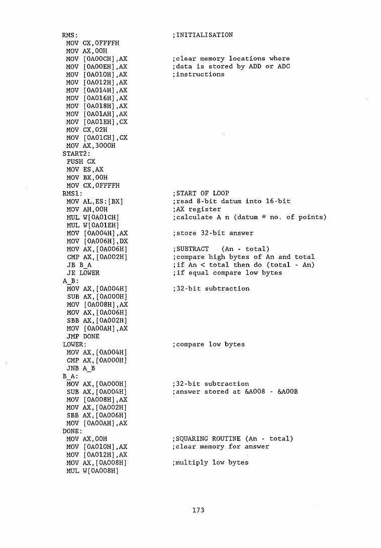
;INITIALISATIONRMS:MOV CX,OFFFFH MOV AX,00H MOV [OAOOCH],AX MOV [OAOOEH],AX MOV [0A010H],AX MOV [0A012H],AX MOV [0A014H],AX MOV [0A016H],AX MOV [0A018H],AX MOV [0A01AH],AX MOV [0A01EH],CX MOV CX,02H MOV [0A01CH],CX MOV AX,3000H START2:PUSH CX MOV ES,AX MOV BX,OOH MOV CX,OFFFFH RMS1:MOV AL,ES:[BX] MOV AH,OOH MUL W[0A01CH] MUL W[0A01EH] MOV [0A004H],AX MOV [0A006H],DX MOV AX,[0A006H] CMP AX,[0A002H] JB B_A JE LOWER

A_B:MOV AX,[0A004H] SUB AX,[OAOOOH] MOV [0A008H],AX MOV AX,[0A006H] SBB AX,[0A002H] MOV [0A00AH],AX JMP DONE LOWER:MOV AX,[0A004H] CMP AX,[OAOOOH] JNB A_B B_A:MOV AX,[OAOOOH] SUB AX,[0A004H] MOV [0A008H],AX MOV AX,[0A002H] SBB AX,[0A006H] MOV [0A00AH],AX DONE:MOV AX,OOH MOV [OAOIOH],AX MOV [0A012H],AX MOV AX,[0A008H] MUL W[0A008H]

;clear memory locations where ;data is stored by ADD or ADC ;instructions

;START OF LOOP;read 8-bit datum into 16-bit ;AX register;calculate A n (datum * no. of points);store 32-bit answer;SUBTRACT (An - total);compare high bytes of An and total ;if An < total then do (total - An);if equal compare low bytes;32-bit subtraction

;compare low bytes

;32-bit subtraction ;answer stored at &A008 - &A00B

;SQUARING ROUTINE (An - total) ;clear memory for answer;multiply low bytes

173

MOV [OAOOCH],AXMOV [0A00EH],DX MOV AX,[0A008H] MUL W[0A00AH] ADD [OAOOEH],AX ADC [OAOIOH],DX JNC NEXT INC B[0A012H]

NEXT

;low times high bytes

MOV AX,[OAOOAH] MUL W[0A008H] ADD [OAOOEH],AX ADC [OAOIOH],DX JNC HIGH INC B[0A012H]

HIGH

;low times high bytes

MOV AX,[OAOOAH] MUL W[OAOOAH]

;multiply high bytes

ADD [OAOIOH],AX ADC [0A012H],DX MOV AX,[OAOOCH] ADD [0A014H],AX MOV AX,[OAOOEH] ADC [0A016H],AX MOV AX,[OAOIOH]

;32*32-bit multiplication ref ;The 8086 Book ,Rector and Alexy ;SUMMATION sigma(An - total)

ADC [0A018H],AX MOV AX,[0A012H] ADC [0A01AH],AX

;64-bit addition

INC BX DEC CX JCXZ FIN1 JMP RMS1 FIN1:POP CXMOV AX,4000H DEC CX JCXZ FIN2 JMP START2 FIN2:

;BX=BX+1 to access next data point ;decrement loop counter ;if CX=0 then finish ;repeat loop

RETF ;return to BASIC program

174

GAMMA4.DG - intermittency and conditional sampling routine

175

GAMMA:MOV AL,2 MOV [0A018],AL MOV AX,00H MOV BX,0A01AH MOV CX,ODH CLEAR:MOV [BX],AX INC BX INC BX LOOP CLEAR MOV AX,3000H MOV CX,02H START3:PUSH CX MOV ES,AX MOV BX,00H MOV CX,0FFF6H GAMMA1:MOV AX,00H MOV [OAOIEH],AX MOV [0A030H],AX MOV DL,OEH SUM1:MOV AL,ES:[BX+1] MOV AH,00H MOV [0A01CH],AX MOV AL,ES: [BX] MOV AH,00H SUB AX,[0A01CH] JNS POS1 NEG AX POS1:ADD [OAOIEH],AX INC BX DEC DL JNZ SUM1 MOV DL,OEH RESET1:DEC BX DEC DL JNZ RESET1 MOV DL,ODH SUM:MOV AL,ES:[BX+1] MOV AH,OOH MUL B[0A018H]MOV [0A01CH],AX MOV AL,ES:[BX] MOV AH,OOH MOV [0A01AH],AX MOV AL,ES:[BX+2] ADD AX,[0A01AH] SUB AX,[0A01CH] JNS POS NEG AX

;INITIALISATION

;clear memory locations which ;receive data via ADD or ADC ;instructions

;clear BX register ;load loop counter with 65526 ;START OF MAIN LOOP ;clear memory locations which ;hold "SUM1" and ,,SUM2";load DL with 14 to control sub-loop ;SUM1 first derivative

;SUM2 second derivative ;load the byte at i+1 into;2*Ui+l;memory location &A01C ;load the byte at i into the ;AX register

;subtract;ensure the absolute value is returned

176

POS:ADD [0A030H],AX INC BX DEC DL JNZ SUM MOV DL,ODH RESET:DEC BX DEC DL JNZ RESET MOV AX,[OAOIEH] CMP AX,1AH JBE LAMINAR MOV AX,[0A030H] CMP AX,1AH JA TURBULENT LAMINAR:MOV AL,ES:[BX+6] MOV AH,00H ADD [0A020H],AX ADC [0A022H],00H MOV AX,001H ADD [0A024H],AX ADC [0A026H],00H JMP LAMI TURBULENT:MOV AL,ES:[BX+6] MOV AH,OOH ADD [0A028H],AX ADC [0A02AH],00H MOV AX,001H ADD [0A02CH],AX ADC [0A02EH],00H LAMI:INC BX DEC CX JCXZ FINISH JMP GAMMAl FINISH:POP CX MOV AX,4000H DEC CX JCXZ FIN3 JMP START3 FIN3:RETF

;add into "SUM2"

;loop 14 times ie. 15 points ;loop 9 times to restore BX

;load "SUM1" into AX register ;compare with 26 ;if "SUM" < 26 then LAMINAR ;load "SUM2" into AX;ie. if SUM1 and SUM2 > 2 6 then TURB;load the value at i+6 into AX;add the value to laminar total ;32-bit addition;add 1 to laminar counterljump to end of loop ;same procedure if point is ;considered turbulent

;inc BX by one

177

DGDATA5.BAS - data acquisition program

178

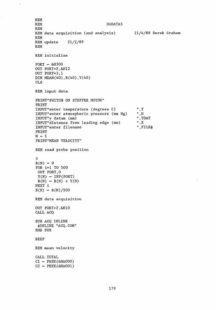
REMREM DGDATA5REMREM data acquisition (and analysis) 21/4/88 Derek GrahamREMREM update 21/2/89 REMREM initialisePORT = &H300OUT PORT+2,&H12OUT PORT+3,1DIM MEAN(40),B(40),Y(40)CLSREM input dataPRINT”SWITCH ON STEPPER MOTOR"PRINTINPUT"enter temperature (degrees C) ",TINPUT"enter atmospheric pressure (mm Hg) ",HINPUT"y datum (mm) ”,YDATINPUT"distance from leading edge (mm) ",XINPUT"enter filename ",FILE$PRINT N = 1PRINT"MEAN VELOCITY"REM read probe position 5B(N) - 0 FOR i=l TO 500 OUT PORT,0 Y(N) = INP(PORT)B(N) = B(N) + Y(N)

NEXT iB(N) = B(N)/500REM data acquisitionOUT PORT+2,&H10 CALL ACQSUB ACQ INLINE 4INLINE "ACQ.COM"

END SUBBEEPREM mean velocityCALL TOTALCl = PEEK(&HA000)C2 = PEEK(&HA001)

179

C3 = PEEK(&HA002)C4 = PEEK(&HA003)TOTAL = C4*(24) + C3*(26) + C2*256 + ClMEAN(N) = TOTAL/(65535*2)REM convert to m/sMEAN(N) = MEAN(N)/12.5SUB TOTAL INLINE $INLINE "TOTAL.COM"

END SUBREM dump data to disc DEF SEG=&H3000BSAVE FILE$+STR$(2*N-1),0,&HFFFF DEF SEG=&H4000BSAVE FILE4+STR4(2*N),0,&HFFFF DEF SEGREM print mean velocityPRINT INT(MEAN(N)*1000+0.5)/1000REM test for profile completed IF N < 2 GOTO 420IF MEAN(N)>=0.995*MEAN(N-1) AND MEAN(N)<=1.005*MEAN(N-1) GOTO 410GOTO 420410IF MEAN(N)>=0.995*MEAN(N-2) AND MEAN(N)<=1.005*MEAN(N-2) GOTO 500 420OUT PORT+2,&H12 N = N + 1IF N < 8 THEN TRAV =0.5 ELSEIF N < 13 THEN TRAV =1.0 ELSETRAV = 2 END IF OUT PORT+3,0 DELAY TRAV OUT PORT+3,1 GOTO 5500REM freestream turbulenceUINF = (MEAN(N) + MEAN(N-l) + MEAN(N-2))/3TINT = 100*RMS(N)/UINFPRINTPRINT"UINF ",UINF

180

PRINTPRINTMN ",NPRINTREM save data to disk file0PEN"0",£1,FILE$WRITE£1,T,H,N,UINF,YDAT,X ,TINT FOR 1=1 TO N WRITEfl,B(I)NEXT I CLOSE£l

END

181

DGDATA6.BAS - data reduction program

182

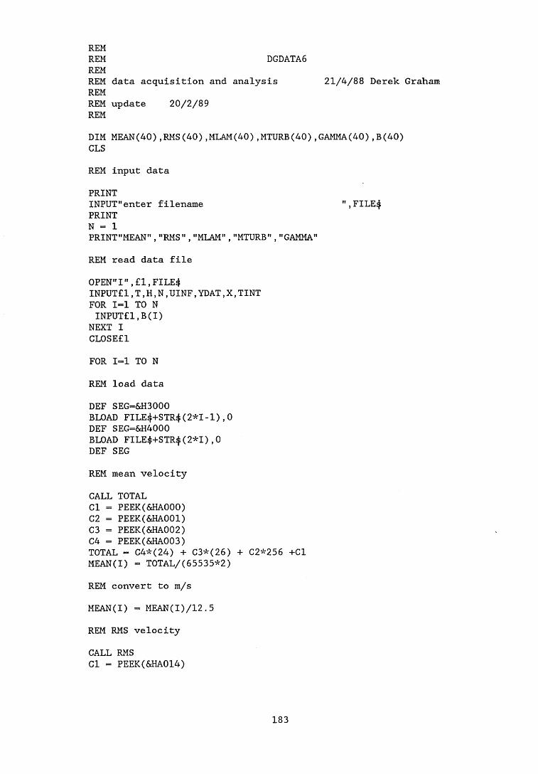
REMREM DGDATA6REMREM data acquisition and analysis 21/4/88 Derek GrahamREMREM update 20/2/89 REMDIM MEAN(40),RMS(40),MLAM(40),MTURB(40),GAMMA(40),B(40)CLSREM input data PRINTINPUT"enter filename ",FILE$PRINT N = 1PRINT"MEAN","RMS","MLAM","MTURB","GAMMA"REM read data fileOPEN"I",£1,FILE#INPUT£1,T,H,N,UINF,YDAT,X ,TINT FOR 1=1 TO N INPUT£1,B(I)

NEXT I CL0SE£1FOR 1=1 TO NREM load dataDEF SEG=&H3000BLOAD FILE4+STR4(2*1-1),0DEF SEG=&H4000BLOAD FILE$+STR4(2*1),0DEF SEGREM mean velocityCALL TOTALCl = PEEK(&HA000)C2 = PEEK(&HA001)C3 = PEEK(&HA002)C4 = PEEK(&HA003)TOTAL = C4*(24) + C3*(26) + C2*256 +C1 MEAN(I) = TOTAL/(65535*2)REM convert to m/s MEAN(I) = MEAN(I)/12.5REM RMS velocity CALL RMSCl = PEEK(&HA014)

183

C2 - PEEK(&HA015)C3 = PEEK(&HA016)C4 = PEEK(&HA017)C5 = PEEK(&HA018)C6 = PEEK(&HA019)C7 - PEEK(&HA01A)C8 = PEEK(ScHAOlB)CA = C8*(26) + C7*(28) + C6*(20) + C5*(22) CB = C4*(24) + C3*(26) + C2*256 + Cl C - CA + CB D = C/(65535*2)E = SQR(D)RMS(I) = E/(65535*2)REM convert to m/s RMS (I) = RMS(I)/12.5REM intermittencyCALL GAMMAVL1 = PEEK(&HA020)VL2 = PEEK(&HA021)VL3 = PEEK(&HA022)VL4 - PEEK(&HA023)VLAM = VL4*(24) + VL3*(26) + VL2*(2) + VL1 CL1 = PEEK(&HA024)CL2 = PEEK(&HA025)CL3 = PEEK(&HA026)CL4 = PEEK(&HA027)CLAM = CL4*(24) + CL3*(26) + CL2*(2) + CL1 VT1 = PEEK(&HA028)VT2 - PEEK(&HA029)VT3 = PEEK(&HA02A)VT4 = PEEK(&HA02B)VTURB - VT4*(24) + VT3*(26) + VT2*(2) + VT1 CT1 = PEEK(&HA02C)CT2 = PEEK(&HA02D)CT3 = PEEK(&HA02E)CT4 = PEEK(&HA02F)CTURB = CT4*(24) + CT3*(26) + CT2*(2) + CT1IF CTURB = 0 GOTO 10MTURB(I) = VTURB/CTURB10 IF CLAM - 0 GOTO 20MLAM(I) - VLAM/CLAM20 GAMMA(I) = CTURB/(65526*2)REM convert to m/sMLAM(I) - MLAM(I)/12.5 MTURB(I) = MTURB(I)/12.5

REM print out results BEEP

184

PRINT INT(MEAN(I)*1000+0.5)/1000,INT(RMS(I)*1000+0.5)/1000,; PRINT INT(MLAM(I)*1000+0.5)/1000,INT(MTURB(I)*1000+0.5)/1000, PRINT INT(GAMMA(I)*1000+0.5)/1000

NEXT I 500REM freestream turbulenceUINF = (MEAN(N) + MEAN(N-l) + MEAN(N-2))/3TINT = 100*RMS(N)/UINFPRINTPRINT"UINF ",UINFPRINTPRINT"N ",NPRINTREM save data to disk fileOPEN"0",£1,FILE$WRITEfl,T,H,N,UINF,YDAT,X ,TINT FOR 1=1 TO NWRITEfl,MEAN(I),RMS(I),MLAM(I),MTURB(I),GAMMA(I),B(I) NEXT I CLOSEflSUB TOTAL INLINE 4INLINE "TOTAL.COM"

END SUBSUB RMS INLINE 4INLINE "RMS2.COM"

END SUBSUB GAMMA INLINE 4INLINE "GAMMA4.COM"

END SUB

END

185

DATA9.BAS - intermittency display program

186

REMREM data analysis program 23/3/88 Derek GrahamREMREM update 13/13/89 Sl(t) AND S2(t) criterion REMINPUT"no. of points for intermittency calculations";PTS INPUT"CUT OFF ";CUT INPUT"factor for sum";FTREM read dataPORT = &H300 OUT PORT+2,&H10 print"reading data"CALL ACQ N = &H00 BEEP5 INPUT XIF X = 99 GOTO 200REM Mean velocityCLSPRINT"Calculating mean velocity"N = X VEL = 0 FOR i=l TO 640 P% = PEEK(N)VEL = VEL + P%N=N+1 NEXT iMEAN - VEL /640REM rms velocityBEEPCLSPRINT"Calculating RMS velocity" N = X TOT = 0FOR k=l TO 640 A% = PEEK(N)B = (A% - MEAN)N = N + 1 TOT = TOT + B

NEXT k C = TOT/640 RMS - SQR(C)BEEPREM set up graph

DEF SEG=&H3000

187

CLS N = X SCREEN 2LINE(0,180)-(640,180)LINE(0,180)-(0,0)LINE(0,80-CUT/FT)-(640,80-CUT/FT)FOR i=l TO 640 P% = PEEK(N)PSET(i,(180-P%/2.4))N - N + 1 NEXT iREM intermittency and mean laminar and turbulent velocities BEEPDIM VEL(300)VTURB = 0 VLAM = 0 CTURB = 0 CLAM = 0 N = XFOR i=l TO 640 FOR F=0 TO PTS-1 VEL(F+1) = PEEK(N+F)NEXT F SUM1 = 0 SUM2 = 0FOR Q=1 TO PTS-1 S = ABS(VEL(Q+1) - VEL(Q))SUM1 = SUM1 + S

NEXT QFOR Q=2 TO PTS-1S - ABS(VEL(Q+1) - 2*VEL(Q) + VEL(Q-l)) REM (VEL(Q+1)-VEL(Q)) SUM2 = SUM2 + S

NEXT QPSET(i+INT(PTS/2),80-SUM1/FT)PSET(i+INT(PTS/2),80-SUM2/FT)IF SUM1 > CUT AND SUM2 > CUT GOTO 10 VLAM = VLAM + VEL(13)CLAM = CLAM + 1 GOTO 2010 VTURB = VTURB + VEL(INT(PTS/2))CTURB = CTURB + 1LINE(i+INT(PTS/2),190)-(i+INT(PTS/2),180)20 N = N + 1

NEXT iIF CTURB = 0 GOTO 30 MTURB = VTURB/CTURB 30 IF CLAM = 0 GOTO 40 MLAM = VLAM/CLAM 40 GAMMA = CTURB/640 INPUT YREM convert to volts MEANV = MEAN/50

188

RMSV = RMS/50 MTURBV = MTURB/50 MLAMV = MLAM/50 BEEPPRINT:PRINT:PRINTPRINT"Mean velocity ",INT(MEANV*100+0.5)/100;"Volts"PRINTPRINT"RMS velocity PRINTPRINT"Mean turbulent velocity PRINTPRINT"Mean laminar velocity PRINTPRINT"Intermittency GOTO 5 200 STOP END

", GAMMA",INT(MLAMV*100+0.5)/100;"Volts"",INT(MTURBV*100+0.5)/100;"Volts"

tf,INT(RMSV*100+0.5)/100;"Volts

189

PROFILE.BAS - profile data display program

190

PROFILEREM REM REM REM REMREM update 17/1/89 REM

b.l. profile display 28/4/88 Derek Graham

REM read data from diskDIM MEAN(40) ,MLAM(40) ,MTURB(40) ,GAMMA(40) ,B(40) ,UM(40) ,UL(40) DIM UT(40),Y(40),Y1(40),RMS(40)INPUT"enter filename ",FILE$OPEN"I",£1,FILE$INPUTfl,T,H,N,UINF,YDAT,X ,TINT FOR 1=1 TO NINPUTfl,MEAN(I),RMS(I),MLAM(I),MTURB(I),GAMMA(I),B(I)

NEXT I CLOSEflREM convert bits in B(n) to mm in Y(n)FOR 1=1 TO NY(I) = YDAT + 0.1979*(B(1) - B(I))NEXT IREM convert velocities to dimensionless quantities based on UINF

FOR 1=1 TO N UM(I) = MEAN(I)/UINF UL(I) = MLAM(I)/UINF UT(I) = MTURB(I)/UINF NEXT IREM estimate §FOR 1=1 TO N IF UM(I) <0.99 GOTO 100DELTA = Y(I) - (Y(I)-Y(I-l))*(UM(I) - 0.99)/(UM(I) - UM(I-l)) GOTO 110 100

NEXT I 110REM non dimensionalise YFOR 1=1 TO N Y1(I) = Y (I)/DELTA NEXT IREM estimate gamma (averaged up to y/delta = 0.4)GAMMA = 0 FOR 1=1 TO N IF Yl(l) >0.4 GOTO 150

191

IF Y1(I) >0.4 GOTO 140 GAMMA = GAMMA + GAMMA(I)

NEXT I 140GAMMA = GAMMA/(I-1) : GOTO 160 150GAMMA = GAMMA(l)160REM graphics outputSCREEN 2 200 CLSPRINT"delta = ", DELTA PRINTPRINT" MENU"PRINTPRINT"LAMINAR PROFILE 1" PRINT"TURBULENT PROFILE 2" PRINT"MEAN PROFILE 3" PRINT"LAMINAR AND TURBULENT PROFILES 4" PRINT"ALL THREE 5" PRINT"INTERMITTENCY 6" PRINT "GAMMA / KLEBANOFF 7" PRINT "RMS 8" PRINT"PRINT OUT DATA AND END 9"INPUT A CLSLINE(55,180)-(555,180)LINE(55,180)-(55,30)LINE(55,30)-(60,30)LINE(355,180)-(355,177)LINE(455,180)-(455,177)LINE(555,180)-(555,177)LOCATE 2,1 : PRINT"y/delta";LOCATE 5,5 : PRINT"1";IF A = 1 THEN GOSUB 500 : GOTO 300IF A = 2 THEN GOSUB 600 : GOTO 300IF A = 3 THEN GOSUB 700 : GOTO 300IF A = 4 THEN GOSUB 500:GOSUB 600IF A = 5 THEN GOSUB 500:GOSUB 600:GOSUB 700IF A = 6 THEN GOSUB 800IF A = 7 THEN GOSUB 900IF A = 8 THEN GOSUB 1000IF A - 9 GOTO 1100300INPUT AIF A - 99 THEN STOPGOTO 200500FOR 1=1 TO NLINE(300*UL(I-l)+55,(180-150*Y1(I-1)))-

(300*UL(I)+55,(180-150*Y1(I))) CIRCLE(300*UL(I)+55,(180-150*Y1(I))),3

NEXT I

192

LOCATE 2,40 : PRINT"Lam"LOCATE 24,45 : PRINT"1";LOCATE 23,75 : PRINT"u/U"RETURN600FOR 1=1 TO NLINE(155+300*UT(I-1),(180-150*Y1(I-1)))-

(155+300*UT(I),(180-150*Y1(I))) CIRCLE(155+300*UT(I),(180-150*Y1(I))),3

NEXT ILOCATE 2,52 :PRINT"Turb"LOCATE 24,57 : PRINT"1";LOCATE 23,75 : PRINT"u/U"RETURN700FOR 1=1 TO NLINE(25 5+3 00*UM(I-1),(180-150*Y1(I-1)))-

(2 5 5+3 00*UM(I),(180-150*Y1(I))) CIRCLE(255+300*UM(I),(180-150*Y1(I))),3

NEXT ILOCATE 2,65 : PRINT"Mean"LOCATE 24,70 : PRINT"1";LOCATE 23,75 : PRINT"u/U"RETURN800CIRCLE(300*GAMMA(l)+55,(180-150*Y1(1))),3 FOR 1=2 TO NLINE(300*GAMMA(I-l)+55,(180-150*Y1(I-1)))-

(300*GAMMA(I)+55,(180-150*Y1(I))) CIRCLE(300*GAMMA(I)+55,(180-150*Y1(I))),3 NEXT ILOCATE 5,60 : PRINT"gamma = ";GAMMA;LOCATE 24,45 : PRINT"1";LOCATE 23,75 : PRINT"gamma"RETURN900PSET(355,180)FOR 1=1 TO 25 YOD = 1/20 Cl = YOD C2 = Cl*5 C3 = 1 + C2 GAM1 = 1/C3X = 300*GAM1 Y = 150*YODLINE -(X+55,180-Y)

NEXT IIF GAMMA = 0 GOTO 910XI = 300*GAMMA(1)/GAMMA +55 : Y1 = 180 - 150*Y1(1)CIRCLE(XI,Yl),3 PSET(X1,Yl)FOR 1=2 TO NXI = 300*GAMMA(I-1)/GAMMA + 5 5 : Yl = 180-150*Y1(I-1)X2 = 300*GAMMA(I)/GAMMA +55 : Y2 = 180-150*Y1(I)PSET(X2,Y2)CIRCLE(X2,Y2),3

193

NEXT I 910LOCATE 5,60 : PRINT"gamma = GAMMA;LOCATE 24,45 : PRINT"1";LOCATE 23,75 : PRINT"gamma"RETURN1000CIRCLE(3000*RMS(l)+55,(180-150*Y1(1))),3 FOR 1=2 TO NXI = (3000*RMS(I-l)/UINF+55)Y1 = (180-150*Y1(I-1))X2 = (3000*RMS(I)/UINF+55)Y2 = (180-150*Y1(I))LINE(XI,Y1)-(X2,Y2)CIRCLE(3000*RMS(I)/UINF+55,(180-150*Y1(I))),3

NEXT ILOCATE 24,44 : PRINT"10%";LOCATE 23,75 : PRINT"RMS"RETURN1100CLSPRINT"Y","Y/DELTA","UM","GAMMA"PRINTFOR 1=1 TO NPRINT INT(Y(I)*1000+0.5)/1000,INT(Yl(I)*1000+0.5)/1000,; PRINT INT(UM(I)*1000+0.5)/1000,INT(GAMMA(I)*1000+0.5)/1000

NEXT IPRINTPRINT"turbulence intensity ",TINT,"%"STOP

194

ANLYS4.BAS - profile reduction program(outputs integral parameters)

195

REM ANALYSIS (anlys4)REMREMREM profile analysis program 5/5/88 Derek GrahamREMREMREM update 16/8/89 REM

modified intermittency analysis

REM read in profile dataDIM MEAN(40),MLAM(40),MTURB(40),GAMMA(40),BI(40),Y(40) DIM RMS(40),UM(40),UL(40),UT(40),Y1(40),U(40)

INPUT"enter filename ",FILE4OPEN"I",£1,FILE^INPUTfl,T,H,N,UINF,YDAT,X ,TINT FOR 1=1 TO NINPUTfl,MEAN(I),RMS(I),MLAM(I),MTURB(I),GAMMA(I),BI(I)

NEXT I CLOSEflREM convert bits(B) to mm(Y)FOR 1=1 TO NY1(I) = YDAT + 0.1979*(BI(1) - BI(I))NEXT IREM non dimensionalise velocities using UINFFOR 1=1 TO N UM(I) = MEAN(I)/UINF UL(I) = MIAM(I)/UINF UT(I) = MTURB(I)/UINF NEXT IREM estimate deltaFOR 1=1 TO N IF UM(I) <0.99 GOTO 100DELTA = Y1(I) - (Y1(I)-Yl(I-l))*(UM(I) - 0.99)/(UM(I) - UM(I-l))GOTO 110 100

NEXT I 110REM non dimensionalise yFOR 1=1 TO N Y(I) = Y1(I)/DELTA NEXT IREM evaluate fluid propertiesMU = (1.725 + 0.004375*T)/1E5 RHO = (0.46535*H)/(T+273)

196

NU = MU/RHOREM calculate Rx RX = UINF*X/(NU*1000)REM estimate gamma (up to y/delta = 0.4)GAMMA = 0 FOR I = 1 TO N IF Y(l) >0.4 GOTO 210 IF Y(I) > 0.4 GOTO 200 GAMMA = GAMMA + GAMMA(I)

NEXT I 200GAMMA = GAMMA/(1-1) : GOTO 220 210GAMMA = GAMMA(l)220

REMLPRINT"FILE NAME LPRINT LPRINTLPRINT"b.1. thickness LPRINT"Intermittency LPRINT"freestream velocity LPRINT"Reynolds number (x)LPRINT LPRINTIF GAMMA <0.01 THEN GOSUB 400:GOSUB 1000:GOSUB 3000 : GOTO 300

: REM LaminarIF GAMMA >0.99 THEN GOSUB 500:GOSUB 2000:GOSUB 4000 : GOTO 300

: REM TurbulentGOSUB 1000GOSUB 2000 : REM transitionalLPRINTGOSUB 5000LPRINTLPRINT"TRANSITIONAL MEAN PROFILE"LPRINT"_________________________"LPRINT

"FILE4

",INT(DELTA*100+0.5)/100 ",INT(GAMMA*1000+0.5)/1000 ",INT(UINF*100+0.5)/100 ",INT(RX*100+0.5)/100

IF GAMMA <0.5 THEN GOSUB 350:GOSUB 400:GOSUB 1000:GOSUB 3000: GOTO 300

GOSUB 350:GOSUB 500:GOSUB 2000:GOSUB 4000

300STOP350OPEN"I",£1,FILE^INPUT£1,T,H,N,UINF,YDAT,X ,TINT

197

FOR 1=1 TO NINPUT£1,MEAN(I),RMS(I),MLAM(I),MTURB(I),GAMMA(I),BI(I)

NEXT I CLOSEflREM convert bits(B) to mm(Y)FOR 1=1 TO NY1(I) = YDAT + 0.1979*(BI(1) - BI(I))NEXT IREM non dimensionalise velocities using UINFFOR 1=1 TO N UM(I) = MEAN(I)/UINF UL(I) = MLAM(I)/UINF UT(I) = MTURB(I)/UINF NEXT IREM non dimensionalise yFOR 1=1 TO N Y(I) = Y1(I)/DELTA NEXT I400FOR 1=1 TO N MLAM(I) = MEAN(I)UL(I) = UM(I)NEXT I RETURN500FOR 1=1 TO N MTURB(I) = MEAN(I)UT(I) = UM(I)NEXT I RETURN1000REMREM laminar b.l. subroutine REMREM calculate shear stressT0L = MU*MLAM(1)/Y1(1)*1000 CFL = 2*TOL/(RHO*UINF)1110REM LAMINAR PARINTSUM1 = 0 SUM2 = 0 SUM3 = 0

198

SUM4 - 0 SUM5 = 0N2 = N - 2 L% = 0CALL SUMS(UL(),N,L%)REM laminar b.l. parametersDEL1L = SUM2THETAL = SUM1 - SUM3DEL2L - SUM1 - SUM4H12L = DEL1L/THETALH32L = DEL2L/THETALRDISL = (UINF*DEL1L)/(NU*1000)RMOML - (UINF*THETAL)/(NU*1000)DEL1LM = DEL1L - GAMMA*SUM5 1800RETURN2000

REMREM turbulent b.l. routine REMDIM UTAU(30),ITUT(30),YPLUS(30),UPLUS(30),E(30)51 = 052 = 053 = 054 = 0 SUM1 = 0 SUM2 = 0 SUM3 == 0 SUM4 = 0 SUM5 = 0REM "loglaw" establish utau & velocity profilesREM in terms of u+ and y+SUM = 0 L = 0 2150FOR 1=1 TO NIF MTURB(I) = 0 GOTO 2450 UTAU(I) = 1 GOTO 2200 2190UTAU(I) = ITUT(I)2200YPLUS(I) = UTAU(I)*Y1(I)/(NU*1000)

199

ITUT(I) = MTURB(I)/(2.439*LOG(YPLUS(I))+5.2)E(I) = UTAU(I) - ITUT(I)IF ABS(E(I)) < 0.00001 THEN GOTO 2300GOTO 21902300IF YPLUS(I) <= 30 OR Y(I) >=0.2 GOTO 2400 L = L + 1SUM = SUM + UTAU(I)2400

NEXT I 2450IF L = 0 THEN GOTO 2510 UTAU1 = SUM/L FOR 1=1 TO NUPLUS(I) = MTURB(I)/UTAU1 YPLUS(I) = UTAU1*Y1(I)/(NU*1000)NEXT IYT1 = YPLUS(3)IF YT1 > 50 GOTO 2500FOR K=2 TO N Yl(K-l) = Y1(K)MTURB(K-l) = MTURB(K)Y(K-l) = Y(K)UT(K-l) = UT(K)NEXT K Y1(N) = 0 MTURB(N) = 0 Y(N) = 0 UT(N) = 0 N = N - 1LPRINT"point nearest the wall has been deleted"GOTO 21502500REM "wallint" establish the inner profile integral functions up to REM and including the third data pointCl = 540.6 C2 = 6546 C3 = 82770 A = 2.439 B = 5.2Pill = A*(YT1*(LOG(YT1)-1)-50*(LOG(50)-1))PI12 = B*(YTl-50)INT1W = PI11+PI12PI21 = YTl*(LOG(YTl))-50*(LOG(50))PI22 = -2*(YT1*(L0G(YT1)-1)-50*(LOG(50)-1))PI23 = 2*A*B*(YT1*(LOG(YT1)-1)-50*(LOG(50)-1))PI24 = B*(YTl-50)INT2W = A*(PI21+PI22)+PI23+PI24PI31 = YT1*(L0G(YT1))-3*YT1*(L0G(YT1))+6*YT1*(L0G(YT1)-1)PI32 = -50*(LOG(50))+3*50*(LOG(50))-6*50*(LOG(50)-1)PI33 = YT1*(LOG(YT1))-50*(LOG(50))PI34 = -2*(YT1*(L0G(YT1)-1)-50*(LOG(50)-1))PI35 = 3*A*B*(YT1*(LOG(YT1)-1)-50*(LOG(50)-1))

200

PI36 - B*(YTl-50)INT3W = A*(PI31+PI32)+3*B*A*(PI33+PI34)+PI35+PI3651 - (Cl + INT1W)*(NU/UINF)*100052 = (YT1*(NU/UTAU1)*1000) - SI53 = (C2 + INT2W)*(NU/UINF)*(UTAU1/UINF)*100054 = (C3 + INT3W)*(NU/UINF)*(UTAU1/UINF)*1000REM "parint" complete integration from third data point REM to the edge of th b .1.L% = 3 GOTO 2520 2510 LPRINTLPRINT"Simpsons rule is used from the wall"LPRINT L% = 0 2520N2 = N - 2CALL SUMS(UT(),N ,L%)

REM total integralsSUM1 = SUM1 + SI SUM2 = SUM2 + S2 SUM3 = SUM3 + S3 SUM4 - SUM4 + S4 SUM5 - SUM5 + S2REM turbulent b.l. parametersDEL1T - SUM2THETAT - SUM1 - SUM3DEL2T = SUM1 - SUM4H12T - DEL1T/THETATH32T = DEL2T/THETATRDIST = (UINF*DEL1T)/(NU*1000)RMOMT = (UINF*THETAT)/(NU*1000)CF1 = 0.246/(EXP(1.561*H12T)*RMOMT.268)CF2 = 2.0*(UTAU1/UINF)TOT = ((CF1+CF2)/2)*RHO*UINF/2 IF L% = 0 THEN T0T=CFl*RH0*UINF/2: GOTO 2800 WP = 0.205*UINF/UTAU1 - 0.5*LOG(UTAU1*DELTA/(NU*1000))-1.066 2800DEL1TR = DEL1L*(1-GAMMA) + DEL1T*GAMMA DEL1TM = GAMMA*SUM5RETURN3000REM laminar printout LPRINT

201

LPRINT"LAMINAR BOUNDARY LAYER PARAMETERS" LPRINTLPRINT"displacement thicknessLPRINT"momentum thicknessLPRINT"energy thicknessLPRINT"shape factor 12LPRINT"shape factor 32LPRINT"displacement thickness ReynoldsLPRINT"momentum thickness Reynolds noLPRINT"tOLPRINT"cfLPRINT

"INT(DELlL*1000+0.5)/1000 "INT(THETAL*1000+0.5)/1000 "INT(DEL2L*1000+0.5)/1000 "INT(H12L*1000+0.5)/1000 "INT(H32L*1000+0.5)/1000

no"INT(RDISL+0.5)"INT(RMOML+O.5)"INT(T0L*1000+0.5)/1000 "INT(CFL*lE6+0.5)/1E6

RETURN4000REM turbulent printoutLPRINTLPRINTLPRINTLPRINTLPRINTLPRINTLPRINTLPRINTLPRINTLPRINTLPRINTLPRINTLPRINTLPRINTLPRINT

"TURBULENT B.L. PARAMETERS"displacement thickness"momentum thickness"energy thickness"shape factor H12"shape factor H32"displacement thickness Reynolds"momentum thickness Reynolds no"cf Lud/Till"cf log-plot"wall shear stress"wake parameter

"INT(DELlT*1000+0.5)/1000 "INT(THETAT*1000+0.5)/1000 "INT(DEL2T*1000+0.5)/1000 "INT(H12T*1000+0.5)/1000 "INT(H32T*1000+0.5)/1000

no"INT(RDIST+0.5)"INT(RMOMT+O.5)"INT(CFl*lE6+0.5)/1E6 "INT(CF2*lE6+0.5)/1E6 "INT(T0T*1000+0.5)/1000 "INT(WP*1000+0.5)/1000

RETURN

5000REM transitional printout LPRINTLPRINT"TRANSITIONAL B.L. PARAMETERS"LPRINTLPRINT"PARAMETER","LAMINAR","TURBULENT"LPRINT "_____________________________________ "LPRINTLPRINT"disp thk",INT(DELlL*1000+0.5)/1000,INT(DELlT*1000+0.5)/1000 LPRINT"mom thk",INT(THETAL*1000+0.5)/1000,INT(THETAT*1000+0.5)/1000 LPRINT"energy thk",INT(DEL2L*1000+0.5)/1000,INT(DEL2T*1000+0.5)/1000 LPRINT"HI2",INT(H12L*1000+0.5)/1000,INT(H12T*1000+0.5)/1000 LPRINT"H32",INT(H32L*1000+0.5)/1000,INT(H32T*1000+0.5)/1000 LPRINT"Rdisp",INT(RDISL+0.5),INT(RDIST+0.5)LPRINT"Rmom",INT(RM0ML+0.5),INT(RMOMT+0.5)

202

LPRINT"Cf",INT(CFL*lE6+0.5)/lE6,"aa"LPRINT"Cf Lud/till","dd",INT(CFl*lE6+0.5)/lE6 LPRINT"Cf Log-plot”,"dd",INT(CF2*lE6+0.5)/lE6 LPRINT"T0",INT(T0L*1000+0.5)/1000,INT(T0T*1000+0.5)/1000 LPRINT"Wake par.","da",INT(WP*1000+0.5)71000LPRINTLPRINTLPRINT"COMBINED PARAMETERS"LPRINTLPRINT"a) Dhawan and Narasimha" LPRINT"dislacement thickness LPRINTLPRINT"b) Modified intermittency" LPRINT"displacement thicknessRETURN

;INT(DELlTR*1000+0.5)/1000

;INT((DEL1LM+DEL1TM)*1000+0.5)/1000

SUB SUMS(U(1),N ,L%)SHARED SUM1,SUM2,SUM3,SUM4,SUM5,DELTA,N2,Y ()DIM A(30),B(30),C(30),DET(30),INTI(30),INT2(30),INT3(30) DIM INT4(30),INT5(30),INT6(30),INT7(30),INT8(30)DIM INT1TM(30),INT2TM(30)FOR K=L% TO N2IF U(K+2) = 0 GOTO 2700DET1 = l*(Y(K+l)*Y(K+2)-Y(K+2)*Y(K+1))DET2 = Y(K)*(Y(K+2)-Y(K+l))DET3 = Y(K)*(Y(K+2)-Y(K+l))DET(K) = DET1 - DET2 + DET3A1 = U(K)*(Y(K+l)*Y(K+2)-Y(K+2)*Y(K+1))A2 = Y(K)*(U(K+l)*Y(K+2)-U(K+2)*Y(K+l))A3 = Y(K)*(U(K+l)*Y(K+2)-U(K+2)*Y(K+1))A(K) = (A1 - A2 + A3)/DET(K)

B1 = l*(U(K+l)*Y(K+2)-U(K+2)*Y(K+l))B2 = U(K)*(Y(K+2)-Y(K+1))B3 = Y(K)*(U(K+2)-U(K+l))B(K) - (B1 - B2 + B3)/DET(K)Cl = l*(Y(K+l)*U(K+2)-Y(K+2)*U(K+l))C2 = Y(K)*(U(K+2)-U(K+1))C3 = U(K)*(Y(K+2)-Y(K+1))C(K) = (Cl - C2 + C3)/DET(K)Pill - A(K)*(Y(K+l)-Y(K))+B(K)*(Y(K+l)-Y(K))/2 PI12 = C(K)*(Y(K+l)-Y(K))/3 INTI(K) = Pill + PI12PI21 = A(K)*(Y(K+2)-Y(K+l))+B(K)*(Y(K+2)-Y(K+l))/2 PI22 = C(K)*(Y(K+2)-Y(K+l))/3

203

INT2(K) = PI21 + PI22PI31 = (1.0-A(K))*(Y(K+l)-Y(K))-B(K)*(Y(K+l)-Y(K))/2 PI32 = -C(K)*(Y(K+l)-Y(K))/3 INT3(K) = PI31+PI32PI41 = (1.0-A(K))*(Y(K+2)-Y(K+l))-B(K)*(Y(K+2)-Y(K+l))/2 PI42 - -C(K)*(Y(K+2)-Y(K+l))/3 INT4(K) = PI41 + PI42PI51 = A(K)*A(K)*(Y(K+1)-Y(K))PI52 = A(K)*B(K)*(Y(K+1)-Y(K))PI53 = (2*A(K)*C(K)+B(K)*B(K))*(Y(K+l)-Y(K))/3 PI54 = B(K)*C(K)*(Y(K+l)-Y(K))/2 PI55 = C(K)*C(K)*(Y(K+l)-Y(K))/5 INT5(K) = PI51+PI52+PI53+PI54+PI55PI61 = A(K)*A(K)*(Y(K+2)-Y(K+l))PI62 = A(K)*B(K)*(Y(K+2)-Y(K+l))PI63 = (2*A(K)*C(K)+B(K)*B(K))*(Y(K+2)-Y(K+l))/3 PI64 = B(K)*C(K)*(Y(K+2)-Y(K+l))/2 PI65 = C(K)*C(K)*(Y(K+2)-Y(K+l))/5 INT6(K) = PI61+PI62+PI63+PI64+PI65PI71 = A(K)*A(K)*A(K)*(Y(K+1)-Y(K))PI72 = 3*A(K)*A(K)*B(K)*(Y(K+l)-Y(K))/2PI73 = A(K)*(A(K)*C(K)+B(K)*B(K))*(Y(K+1)-Y(K))PI74 = B(K)*(6*A(K)*C(K)+B(K)*B(K))*(Y(K+l)-Y(K))/4 PI75 - 0.6*C(K)*(A(K)*C(K)+B(K)*B(K))*(Y(K+1)-Y(K))PI76 = B(K)*C(K)*C(K)*(Y(K+l)-Y(K))/2 PI77 = C(K)*C(K)*C(K)*(Y(K+l)-Y(K))/7 INT7(K) - PI71+PI72+PI73+PI74+PI75+PI76+PI77PI81 = A(K)*A(K)*A(K)*(Y(K+2)-Y(K+l))PI82 = 3*A(K)*A(K)*B(K)*(Y(K+2)-Y(K+l))/2PI83 = A(K)*(A(K)*C(K)+B(K)*B(K))*(Y(K+2)-Y(K+l))PI84 = B(K)*(6*A(K)*C(K)+B(K)*B(K))*(Y(K+2)-Y(K+l))/4 PI85 = 0.6*C(K)*(A(K)*C(K)+B(K)*B(K))*(Y(K+2)-Y(K+l)) PI86 = B(K)*C(K)*C(K)*(Y(K+2)-Y(K+l))/2 PI87 = C(K)*C(K)*C(K)*(Y(K+2)-Y(K+l))/7 INT8(K) = PI81+PI82+PI83+PI84+PI85+PI86+PI87REM simpsons rule integration for modified disp thkSUM = 0 C=0FOR I=Y(K) TO Y(K+1) STEP (Y(K+1) - Y(K))/10 IF C=0 OR C=10 THEN MUL = 1 : GOTO 2550 IF C/2 = INT(C/2) THEN MUL - 2 ELSE MUL - 4 2550SA = 1 - (A(K) + B(K)*I + C(K)*I)SB = 1 + 5*1 S = SA/SB S = MUL*S SUM = SUM + S C=C+1

204

NEXT IINTITM(K) = SUM*(Y(K+1) - Y(K))/30SUM = 0 C=0FOR I=Y(K+1) TO Y(K+2) STEP (Y(K+2) - Y(K+1))/10 IF C=0 OR C=10 THEN MUL = 1 : GOTO 2560 IF C/2 = INT(C/2) THEN MUL = 2 ELSE MUL = 4 2560 C=C+1SA = 1 - (A(K) + B(K)*I + C(K)*I)SB = 1 + 5*1 S - SA/SB S = MUL*S SUM = SUM + S

NEXT IINT2TM(K) = SUM*(Y(K+2) - Y(K+l))/30IF K = L% GOTOGOTO2600

2610SUM1 - SUM1 +SUM2 = SUM2 +SUM3 = SUM3 +SUM4 = SUM4 +SUM52610

=5 SUM5 +IF K < N2 AND ]GOTO2620

2630SUM1 - SUM1 + iSUM2 = SUM2 + ISUM3 — SUM3 + iSUM4 = SUM4 + iSUM52630

= SUM5 + i

IF K = N2 GOTOGOTO2640

2650SUM1 = SUM1 + iSUM2 = SUM2 + iSUM3 = SUM3 + iSUM4 = SUM4 + iSUM52650

= SUM5 + i

NEXT K

2600

INTI(K) INT3(K) INT5(K) INT7(K) INTITM(K)

GOTO 2620

0.5*(INT3(K) + INT4(K-1)) + INT6(K-l))

0.5*(INT1TM(K) + INT2TM(K-1))

0.5*(INT1(K) + 0.5*(INT3(K) + 0.5*(INT5(K) + 0.5*(INT7(K) +

INT2(K-1)) INT4(K-1)) INT6(K-1)) INT8(K-l))

+ INT2(K) + INT4(K) + INT6(K) + INT8(K)

0.5*(INT1TM(K) + INT2TM(K-1)) + INT2TM(K)

2700SUM1 = DELTA*SUM1 SUM2 = DELTA*SUM2 SUM3 = DELTA*SUM3 SUM4 = DELTA*SUM4 SUM5 = DELTA*SUM5

END SUB

205

CS.BAS - C-S boundary layer calculation method

206

12/9/88REMREM CS-METHOD REMREM Numerical method of Cebeci and Smith (1977)REMREM Revised 18/10/89 REMREM Main controlling program REMREM Dimension arraysDIM X(1001),UE(1001),M(1001),ALPH(1001)DIM H(61),ETA(61),DELV(61),F(61,2),U(61,2),V(61,2),B(61,2)DIM Sl(61),S2(61),S3(61),S4(61),S5(61),S6(61),R1(61),R2(61),R3(61) DIM Wl(61),W2(61),W3(61),All(61),A12(61),A13(61),A21(61),A22(61) DIM A23(61),G11(61),G12(61),G13(61),G21(61),G22(61),G23(61)DIM DELU(61),DELF(61),A(61)REMITMAX = 10 ALPH(l) = 0 NX = 1GOSUB 1000 : REM InputGOSUB 2000 : REM gridGOSUB 3000 : REM Initial profile0PEN"0",£1,FILE*+".DAT”0PEN"0",£2,FILE*+".ERR"0PEN"0",£3,FILE*+".PRO"WRITEfl,FILE*,NXT WRITE£3,NXTPRINT25LOCATE 10,16 : PRINT" X'\X(NX);"m LOCATE 12,16 : PRINT"NX",NXIT = 0RX = UE(NX)*X(NX)/NUIF NX >= NTR-1 AND NX < NTR THEN RXTR = RX IF NX >= NTR AND NX < NTR+1 THEN GOSUB 3500IF NX > 1 THEN ALPH(NX) = 0.5*(X(NX)+X(NX-1) )/(X(NX) -X(NX-l) )Ml = 0.5*(M(NX)+1)ALPH1 = Ml + ALPH(NX)ALPH2 = M(NX) + ALPH(NX)IF NX < NTR THEN STATU* = "Laminar b.l." : GOTO 40IF NX>=NTR AND NX<NTR+1 THEN STATU* = "TRANSITION POINT" : GOTO 40IF NX > NTR AND GAMTR <0.99 THEN STATU* = "Transitional b.l."

ELSE STATUS = "Turbulent b.l."

207

LOCATE 16,16 : PRINT"**** ";STATU$;" ****"IF NX < NTR GOTO 60 GOSUB 4000 : REM Eddy subroutine 60IT = IT+1IF IT>ITMAX THEN PRINT"Max iterations exceeded at x = ";NX;:GOTO 90GOSUB 5000 : REM CMOM GOSUB 6000 : REM S0LV3

40

REM Check for convergence

61IF NX > NTR GOTO 62 REM Laminar flow IF ABS(DELV(l)) > 1.0E-5 GOTO 60 GOTO 75REM Turbulent flow 62IF ABS(DELV(l))/(V(l,2)+0.5*DELV(1)) >0.02 GOTO 60REM check for growth 75IF NX = 1 GOTO 90IF NP = 61 GOTO 90IF ABS(V(NP,2)) < 1.0E-3 GOTO 90GOSUB 7000 : REM growthGOTO 6090GOSUB 8000 : REM output GOTO 251000REMREM input subroutine REMETAE = 8 NU = 1.5E-5 XSTART = 0 XEND =950 ST = 20INPUT"transition location (mm) ";XTRANSINPUT"file name ";FILE4INPUT"freestream turbulence (%) ";TUNXT = (XEND - XSTART)/ST + 1NTR = 1 + (NXT-1)*(XTRANS - XSTART)/(XEND - XSTART)H(l) = 0.01 K = 1.14FOR 1=0 TO NXT-1 X(I+1) = (XSTART + I*ST)/1000 READ UE(I+1)

NEXT I

208

DATA 0,2,4,5.4,7.3,9.4,11,12.4,13,13.2,13.4,13.6,13.8,14,14.2,14.3 DATA 14.4,14.5,14.7,14.8,15,15,15,15,14.8,14.7,14.5,14.4,14.3,14.2 DATA 14.1,13.9,13.8,13.6,13.5,13.4,13.3,13.2,13.1,13,12.9,12.8,12.6 DATA 12.5,12.4,12.4,12.3,12.3,12.3REM calculation of pressure gradient parameter m

M(l) = 11050FOR 1=2 TO NXT IF I = NXT GOTO 1060 A1 = (X(I)-X(I-1))*(X(I+1)-X(I-1))A2 = (X(I)-X(I-1))*(X(I+1)-X(I))A3 = (X(I+1)-X(I))*(X(I+1)-X(I-1))DUDX = -(X(I+1)-X(I))/A1*UE(I-1) + (X(I+1)-2*X(I)+X(I-1))/A2*UE(I)

+ (X(I)-X(I-l))/A3*UE(I+1)GOTO 1070 1060A1 = (X(I-l)-X(I-2))*(X(I)-X(I-2))A2 = (X(I-l)-X(I-2))*(X(I)-x(I-l))A3 = (X(I)-X(I-l))*(X(I)-X(I-2))DUDX = (X(I)-X(I-l))/Al*UE(I-2) - (X(I)-X(I-2))/A2*UE(I-l)

+ (2*X(I)-X(I-2)-X(I-l))/A3*UE(I)1070M(I) = X(I)/UE(I)*DUDX NEXT IRETURN2000REMREM grid subroutine REMIF (K - 1) < 0.001 GOTO 2005NP = LOG((ETAE/H(l))*(K-l)+l)/LOG(K) + 1.0001GOTO 20102005NP = ETAE/H(1) + 1.0001 2010IF NP < 61 GOTO 2015PRINT"NUMBER OF VERTICAL GRID POINTS EXCEEDED 61"STOP2015ETA(l) = 0 FOR J=2 TO 61 H(J) = K*H(J-1)A(J) = 0.5*H(J-l)ETA(J) = ETA(J-l) + H(J-l)

NEXT JRETURN3000REM

209

ETANPQ - 0.25*ETA(NP)ETAU15 = 1.5/ETA(NP)FOR J=1 TO NP ETAB = ETA(J)/ETA(NP)ETAB2 = ETABF(J,2) = ETANPQ*ETAB2*(3 - 0.5*ETAB2)U(J,2) = 0.5*ETAB*(3 - ETAB2)V(J,2) = ETAU15*(1 - ETAB2)B(J , 2) = 1.0

NEXT JRETURN3500REMREM transition point REMRTHTR = RTHETAMTR - -RTHTR*NU*M(NX)/(X(NX)*UE(NX))NO = 0.7 + EXP(0.588 - 3*TU)N = (NO + 22705*MTR*EXP(-0.45*TU))*lE-3 N - 0.0222RLAMBDA = SQR((0.411*RTHTR)/N)LAMBDA = RLAMBDA*NU/UE(NX)PRINTPRINT"lambda = "LAMBDA RETURN4000REMREM eddy subroutine REMGAMTR = 1BETA = (X(NX) - XTRANS/1000)/LAMBDAEXPTM = 0.411*BETAIF EXPTM < 10 GOTO 4015GOTO 40204015GAMTR - 1.0 - EXP(-EXPTM)4020IFLGD = 0 RX2 = SQR(RX)RX4 = SQR(RX2)PPLUS = M(NX)/(RX4*V(1,2).5)RX216 = RX2*0.16CN = SQR(1 - 11.8*PPLUS)CRSQV = CN*RX4*SQR(V(l,2))/26 J = 1EDVO = 0.0168*RX2*(ETA(NP)-F(NP,2) + F(1,2))*GAMTR 4050IF IFLGD = 1 GOTO 4100

REM initial profile subruotineREM

210

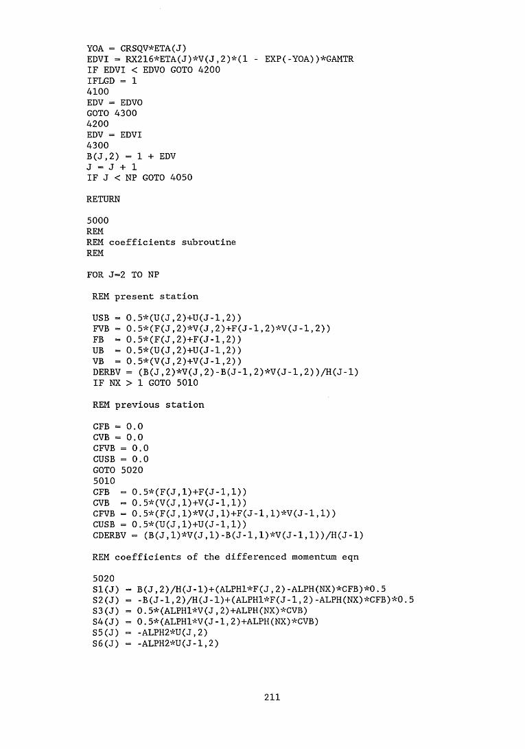
YOA = CRSQV*ETA(J)EDVI - RX216*ETA(J)*V(J,2)*(1 - EXP(-YOA))*GAMTR IF EDVI < EDVO GOTO 4200 IFLGD = 1 4100EDV = EDVO GOTO 4300 4200EDV - EDVI 4300B(J,2) = 1 + EDV J - J + 1IF J < NP GOTO 4050RETURN5000REMREM coefficients subroutine REMFOR J=2 TO NPREM present stationUSB - 0.5*(U(J,2)+U(J-1,2))FVB - 0.5*(F(J,2)*V(J,2)+F(J-1,2)*V(J-1,2))FB - 0.5*(F(J,2)+F(J-1,2))UB - 0.5*(U(J,2)+U(J-1,2))VB = 0.5*(V(J,2)+V(J-1,2))DERBV = (B(J,2)*V(J,2)-B(J-1,2)*V(J-1,2))/H(J-1) IF NX > 1 GOTO 5010REM previous stationCFB =0.0 CVB =0.0 CFVB =0.0 CUSB =0.0 GOTO 5020 5010CFB = 0.5*(F(J,1)+F(J-1,1))CVB = 0.5*(V(J,1)+V(J-1,1))CFVB = 0.5*(F(J,1)*V(J,1)+F(J-1,1)*V(J-1,1))CUSB = 0.5*(U(J,1)+U(J-1,1))CDERBV = (B(J,1)*V(J,1)-B(J-1,1)*V(J-1,1))/H(J-1)REM coefficients of the differenced momentum eqn5020S1(J) = B(J,2)/H(J-1)+(ALPH1*F(J,2)-ALPH(NX)*CFB)*0.5S2(J) = -B(J-1,2)/H(J-1)+(ALPH1*F(J-1,2)-ALPH(NX)*CFB)*0.5 S3(J) = 0.5*(ALPH1*V(J,2)+ALPH(NX)*CVB)S4(J) = 0.5*(ALPH1*V(J-1,2)+ALPH(NX)*CVB)S5(J) = -ALPH2*U(J,2)S6(J) = -ALPH2*U(J-1,2)

211

REM definitions of RJIF NX = 1 GOTO 5030 MIA = 0.5*(M(NX-1)+1)CLB = CDERBV+M1A*CFVB+M(NX-1)*(1 - CUSB)CRB = -M(NX)+ALPH(NX)*(CFVB-CUSB)-CLBGOTO 50355030CRB = -M(NX)5035R2(J) - CRB-(DERBV+ALPH1*FVB-ALPH2*USB-ALPH(NX)*(CFB*VB-CVB*FB)) R1(J) = F(J-1,2)-F(J,2)+H(J-1)*UB R3(J-l) - U(J-1,2)-U(J,2)+H(J-1)*VB

NEXT JRl(l) - 0 R2(l) = 0 R3(NP) = 0RETURN6000REMREM SOLV3 block elimination method REMREM W-Elements for J=1Wl(l) = Rl(l)W2(1) = R2(l)W3(1) = R3(1)REM ALPHA - elements for J=1All(1) = 1.0 A12(1) = 0 A13(1) - 0 A21(l) = 0 A22(1) = 1.0 A23(1) = 0REM GAMMA elements for J=2Gll(2) = -1.0 G12(2) - -0.5*H(1)G13(2) = 0 G21(2) = S4(2)G23(2) = -2*S2(2)/H(1)G22(2) = G23(2)+S6(2)REM Forward sweepFOR J=2 TO NP IF J=2 GOTO 6100

212

213

d ■o d 2d o d ✓—Nds o H X

o - Hro< c: ij o/—\ / N / V 5dOh C_,- - - Oh

<-i k > ro ro ||

< cj hcj/%<h q

ro ro 10w w+ + +

a o o w n w d d d< CJ Hjz' V ON ^Oh Oh Ch

HO

2hd

M O O^ w w , d d«H Tj Cj

V Ch Ch

oOHO

onONOO

s j >M on on C_| «H +

Od

5© M W oo 3N> IIII S3

oo> -p NO ChOh OW \Ti* c

> dM on lO C-i

ONONoo

M > on ro >{•0- i (jo >NO on f—1* Oh !-» !> vo on1— * >f- Oh to > n o

\ on MO O HW VO ONS Ch ro vo

3H/ N2hd

© O d d © W W M H W d d d^ <s ii ii d

S5 2 S3 S| 3hd hd ro (-> hd

2 !2J hJ hd

M M > > WH ro N H^Ni H- to IO !2j> > o\ hd2 “

> * * ■n + U>M hj hdM O Ch M /—N/•—\ o oto d S3 O' o 2 2 * *On f to >£■ + hd hd O OCh < S N > > o ^ w wo /N Oh /-N / s * 1 fH tH* Oh O' Oh Oh © m d aO + + + d i—1 <■—\d I d M M d >5-2 2d d W o o < > t-d hdd U> * i * /■N(O o oon > > o 2 Md to to d hdV/ ro 1-1 d No/ 21 ON /-X < '-- hd> Oh Ch on \ oM v-' Ch > oU) O' >?• + M\on 1 > M MO > M vo on >o ro CO 2 ro* M hd wO Ch od Ch O' 2d o i hd<3 * > oon S3 N *Ch M Oh >'w' / N + MO' Oh M M\ o O' /~N> i * 2t—1 d > hdM <j0 to VO/N >£* to iCh > >o ro + Oh M

3hdv_'

3>roM/ saso

00S9

f 1X

3N(r)en =

(r)£w

(T-f

)efl

*(r

)£3

0-(

T-r

)Zfl

*(f

)Z3

9-(

T-r

)Tfl

*(f

)T3

9-(

f)3

H -

(f

)Ztt

(i

-r)£

^(r

)£i3

-(i-

f)2

^(r

)3T

3-(

i-r

)i^

(r)i

TD

-(r

)iH

=

(r)i

a > > > > > > ON O o Q a o oto to ro r-* M M M to ro to r—1 M MW to M 00 to M O 00 to M w to M/--V<~v /—S x—N/> /~v O Ov Ov OnOh Oh 0h Oh Ch Oh Oh 0h Ch 0h Oh Oh

___' VO v__' v-x v__' v__' vo no VO VO vo

II I II II II II II II II II II II

cn in in > i M O < v Ov Ov 1 ONM On 00 V-v > • to 1 m o

/ v Ch O t—* 00 to M > to0h Ch Ch vo Ch ✓ ~v ro On M On U>O ' vo O ' >{■ Ch ^v Oh Ov Oh on

+ l o l v__' Oh vo Oh vo Ch

> o r—1 Q Hr —/ * vo + 1~v ro 00 H* > + > * O MOh 00 X~N U> M m to > t—1 v-v—' ✓ ~v Oh /*N to ON t—1 t—1 M +* Oh VO Ch /~v ~v ON U) OV >O O ' Vw/ Oh Ch 0h ^N Ch O wto i vo i 0h vo Chu> t—1 * M i X- vo

V VO > vo M Ov *Oh + /*\ 1 NO > '"vV__' O Ch CO + M >

to VO -pv o to ONto 1 On (—1on Ch'--V O 0h to Ch voOh to no Ov > >c-VO M * Oh 1-* >* / v > VO vo fvj> Ch to N' X- Mto vo co > > '"vto >5- Ov to on 0h✓ V x~v Oh OJ Oh iOh > i Ov VO (—*i / V M Ch 1 NO

M Oh NO i > 1VO VO + M M >i * > vo oj tom > Ov NO On roON M Ch \ Ch on^v to vo > i OhOh ON >{■On M >vo Ch On Ch NO |-»

i CO NO NO VOM •pv NO NOvo ON \ vo1 Ch o \> V--' M OM >5- Hr 2 MU> > > M 2ov ro toOh r—1 toi Ov O n

M Oh OhVO i ivo M Mvo VO NO\ v__' 1o VO COM \ ON2 o Ovt—1 w Oh

2 vo

(i-f)£3v-(f)v*(i-f)zzv = iNaa

(((T-r)TTV*(T-f)Z3V-

(T-r)TZV*(T-f)zTv)*(r)v-(T-f)TTv*(T-f)£ZV-(T-r)TZV*(T-f)eiv) -

Naa

NPO = NP NP1 - NP+1 NP = NP+1IF NX = NTR THEN NP - NP + 3 IF NP > 61 THEN NP - 61REM definition of profiles for new npFOR J - NP1 TO NPF(J,1) = U(NP0,1)*(ETA(J)-ETA(NP0))+F(NP0,1)U(J,1) = U(NPO,1)V(J,1) = oB(J,1) = B(NPO,1)F(J ,2) - U(NPO,2)*(ETA(J)-ETA(NPO))+F(NPO,2)U( J ,2) = U(NPO,2)V(J,2) - V(J,1)B(J,2) = B(NPO,2)

NEXT JNNP = NP-(NPl-l)WRITE£2,NX,NNPRETURN8000REMREM output subroutine REMWRITE£3,X(NX),NP,UE(NX)FOR J=1 TO NP WRITE£3,ETA(J),U(J,2)NEXT J

IF NX = 1 GOTO 8210 FI = 0 THETA1 = 0 FOR J=2 TO NP F2 = U(J,2)*(1-U(J,2))THETAl = THETA1+(F1+F2)*0.5*H(J-1)FI = F2

NEXT JTHETA = THETA1*X(NX)/SQR(RX)DELS - (ETA(NP)-F(NP,2))*X(NX)/SQR(RX)H = DELS/THETACF = 2.0*V(1,2)/SQR(RX)RTHETA = UE(NX)*THETA/NU RDELS = UE(NX)*DELS/NUWRITE£1, X(NX) , THETA, DELS, H,CF,RX, RTHETA, RDELS, UE (NX) ,M(NX) , GAMTR

REM Growth subroutineREM

8210NX = NX+1IF NX > NXT THEN CLOSE£l:CLOSE£2:CL0SE£3:END

214

REM shift profilesFOR J-l TO NP F(J,1) - F(J,2) U(J,1) - U(J,2) V(J,1) - V(J,2) B(J,1) - B(J,2)

NEXT J

RETURN

APPENDIX 2

EXPERIMENTAL DATA - INTEGRAL PARAMETERS

216

Rthetaflow 1

Rtheta 1000 n

800 -

600 -

13400 -

200 -

0 —600

D Rth mean A Rth laminar O ftth turbulent

figure A2.1 momentum thickness Re number

700 800x (mm)

O O r, O O

A A

Rtheta flow 2

1000 -i

° Rth mean A Rth laminar O Rth turbulent

figure A2.2 momentum thickness Re number

217

Rthetaflow 3

Rtheta1000 -

800 -

600 -

n400 -

200 -

0 ---------------1-------------600 700

x (mm)

D Rth mean A Hth laminar O Rth turbulent

figure A2.3 momentum thickness Re number

✓■s Q O O O°n° „ O° O Q□

□

2 A A A

Rtheta flow 4

1000Rtheta

800 o° °o °° on 0 O

600

400

2 0 0 -

n abSj

600 700 x (mm)

n Rth mean Rth laminar O Rth turbulent

figure A2f4 momentum thickness Re number

800

800

218

Rthetaflow 5

1000Rtheta

800 -

6Q0

,<XP aOo ° o u DcPo° a

a

Q°□ a

400 *

2 0 0 -

400 600 600 x (mm)

700 800

D Rth mean A Rth laminar ° Rth turbulent

figure A2.5 momentum thickness Re number

Rtheta flow 6

Rtheta

D Rth mean A Rth laminar O Rth turbulent

figure A2.6 momentum thickness Re number

219

shape factorflow 1

H6 i

A -

n

3 -

2 -

1 -

D O 6Aa

A□• A

0 □ A00 Ao D

° 8 ^§ A0

o -t— 600

n H mean A H laminar ° H turbulent

tigure A2.7 shape factor

----1------------------------------- 1700 800

x (mm)

shape factor flow 2

H

a H mean A H laminar ° H turbulent

figure A2.8 shape factor

220

shape factorflow 3

H4 -

tpD □ 6 &

Aa

3 -

2 -

AO

O O oo

AA

ao □ A

o© D O

1 -

0 -t— 800

° H mean ^ H laminar ° H turbulent

figure A2.8 ehape factor

--1---------------- 1700 800

x (mm)

shape factor flow 4

H

D H mean A H laminar ° H turbulent

figure A2.10 ehape factor

221

shape factorflow 5

H

3-i

2 -

1 -

4 -

o4—400

H4 -

3 -

n2-

1 -

o H—400

D

□

n a acaa □ nA A

AA

O ^° °°Qo~c ° o ‘

D

I500

I800

1700

x (mm)

H mean A H laminar ° H turbulent

figure A2.11 shape factor

shape factor flow 6

D V -□ AAa

□ a a an L

o ° o 0 oo° ° o o o 3° 8 0 H“ 8 □□

---------- 1600

\eoo

(700

x (mm)

H mean A H laminar ° H turbulent

figure A2.12 shape factor

222

flow 7velocity distribution

U m/s 25 i

20-

o n

15 -

10-

5 -

0 i------!------1------i------ 1 0 200 400 600 800

x (mm)

D freestream velocity

figure A2.13 velocity distribution for flow 7

1000

223

Rthetaflow 7

Rtheta2000-1

1500-

1000 -

500 -

0 4--- 1--- !--- I--- 1--- 1--- 1--- 1--- 1200 300 400 500 600 700 800 900 1000

x (mm)

° Rth mean A Rth laminar 0 Rth turbulent

figure A2.14 momentum thickness Reynolds number

shape factor flow 7

H

D H mean A H laminar ° H turbulent

figure A2.15 shape factor

2 2 4

APPENDIX 3

EXPERIMENTAL DATA - VELOCITY PROFILES

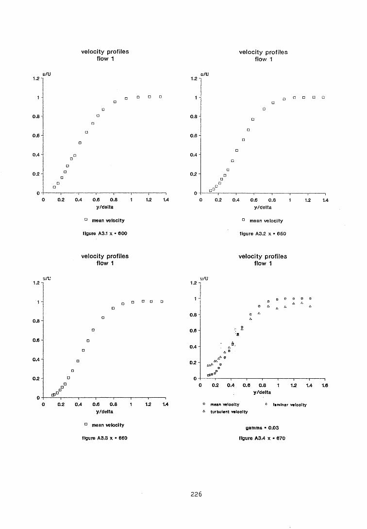
velocity profilesflow 1

velocity profilesflow 1

1.2u/u u/u1.2 ~i

D □ 0 1 - □ Q □ O

0.8 0.8-

0.8 0.6

0.4- 0.4

0.2- 02. -

i ---------- r ~i----1----1----10 0.2 0.4 0.6 0.8 1

y/delta

D mean velocity

figure A3.1 x * 600

1.2 1.4 0 0.2 0.4-i-------------- r

0.6 0.8 1 y/delta

D mean velocity

figure A3.2 x - 650

1.2 1.4

velocity profiles flow 1

velocity profiles flow 1

•j/u u/U

D mean velocity

figure A3.3 x * 660

D mean velocity & turbulent veloolty

0 laminar veloolty

gamma - 0.03

figure A3.4 x - 670

226

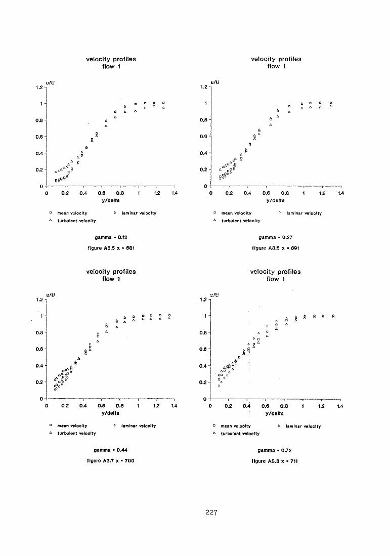
velocity profilesflow 1

1.2-11

0.8

0.6

0.4

0.2

V/U

tA - 6

0 t0.2 0.4 0.6 0.8 1 12 1.4

y/delta

D mean velocity A turbulent velocity

6 laminar velocity

gamma - 0.12

figure A3.5 x ■ 681

velocity profilesflow 1

u /u

a mean velocity A turbulent velocity

A laminar velocity

gamma • 027

tigure A3.6 x ■ 691

velocity profiles flow 1

u/U12-1

a mean veloolty A laminar velocity

A turbulent veloolty

velocity profiles flow 1

.j/ij

D mean veloolty A laminar velocity

A turbulent velocity

gamma ■ 0.44

figure A3.7 x ■ 700

gamma - 0.72

tigure A3.8 x ■ 711

velocity profilesflow 1

velocity profilesflow 1

u/u

D mean veloolty 6 laminar velooltyA turbulent veloolty

1.2 1

1 -

0.8

0.6

O A

0.2

U/U

§ fl fl £j D 6

e 2Ba ;

------ !---------- ,---------- ,---------- 1--------- 1------------r---------- i0 0.2 0.4 0.6 0.8 1 1.2 1.4

y/'delta

c mean veloolty ^ turbulent velocity

0 laminar veloolty

gamma - 0.86

figure A3.9 x • 721

gamma - 0.93

figure A3.10 x « 730

velocity profiles flow 1

velocity profiles flow 1

u/U

D mean velocity 6 laminar veloolty^ turbulent veloolty

u/U

gamma - 0.98 ° mean velocity

figure A3.11 x ■ 760 figure A3.12 x - 781

228

velocity profilesflow 1

u/u12 -i

1 -

o.s-

0.6 -

0.4-

02 -

ao

□ □

0 4- 0— --------------- 1----------------1----------------1—

0 2 0.4 0.6 0.8y/delta

D mean velocity

figure A3.13 x - 800

□ □ □ a

1.2

229

velocity profilesflow 2

velocity profilesflow 2

u/U1.2 l

1 -

0.8

0.8-

0 A -

02

O D D

1.2 1.40 -1--------------:-------------- 1--------------1------- -------1-------------r

0 0.2 0.4 0.6 0.8 1y/delta

a mean velocity

figure A3.14 x - 301

1.2 u /U

0.8

0.6 -

0.4

02

□ □ □ a

i i------- :-------:-------1------- 1------- 1-------10 0.2 0.4 0.6 0.8 1 1.2 1.4 1.6

y/delta

D mean velocity

figure A3.15 x • 401

velocity profiles flow 2

velocity profiles flow 2

1.2 U/U

1 -

0.8

0.6-

0.4

02 -

a a a

\ I0.2 0.4 0.6 0.8 1

y/delta

D mean velocity

figure A3.16 x * 600

—i----11.2 1.4

12 u/U

1 -

0.8 -

0.6 -

0.4

0.2 1

d n a a □

0 -j i i i i i i--- 1---1---10 0.2 0.4 0.6 0.8 1 1.2 1.4 1.6 18

y/delta

° mean velocity

figure A3.17 x ■ 649

230

velocity profilesflow 2

velocity profilesflow 2

1.2 u/U

0.8 n

0.6

0.4

0.2

n c □ □

0 _j-----------1------------1----------- 1------------|----------- ]------------i------------1----------- )

0 0.2 0.4 0.6 0.8 1 1.2 1.4 1.6y/delta

D mean velocity

figure A3.18 x * 600

1.2 u/U

0.8'

0.6-

0.4 -

0.2

□ d n a

a□

'i---------- 1-----------1---------- 1---------- r0.2 0.4 0.6 0.8 1

y/delta

D mean velocity

figure A3.19 x • 660

1.2 1.4

velocity profiles flow 2

velocity profiles flow 2

u/U

D mean velocity

figure A3.20 x • 661

u/U

D mean velocity

figure A3.21 x ■ 668

231

velocity profilesflow 2

velocity profilesflow 2

u/U

0 0.2 0.4 0.6 0.8y/delta

1.2 1.4

D mean velocity a turbulent velocity

* laminar velocity

U/U1.2 -i 1.2 h

1 - a ° 2 2 £n a ^

1 -

0.8- 6 ^ 0.8-A

00.6 - 0.8 -

0 .4 - 6£x 0.4 -

AA 0 a'£r*0 2 - aa 0.2 - A n A

o -gP-

---------- 1---------- !---------- 1-----------1---------- 1---------- 1----------1 o-

CDgS 6

---------- 1—

_ a qC A. S

0.2 0.4 0.6 0.8y/delta

1.2 1.4

D mean velocity a turbulent veloolty

o laminar veloolty

gamma ■ 0.12

figure A3.22 x ■ 680

gamma - 0.28

figure A3.23 x - 691

velocity profiles flow 2

u/U

D mean veloolty 0 laminar veloolty

a turbulent velocity

velocity profiles flow 2

u/u

° mean veloolty 6 laminar velocity

a turbulent veloolty

gamma ■ 0.47

figure A3.24 x ■ 696

gamma • 0.73

figure A3.25 x ■ 700

velocity profilesflow 2

velocity profilesflow 2

1.2

1 -|

0.8

0.8

0.4

0.2

u/U

6 fi a c aft □ A ft D

* eH

-- 1---- 1----1----1--- 1-----1---- 10 0.2 0.4 0.6 0.8 1 1.2 1.4

y/delta

D mean velocity ^ laminar velocity“ turbulent velocity

1

0.8 H

0.8

0.4

02

1.2 u /U

k a n O 6 6

ftS

0.2 0.4 0.6 0.8y/delta

1.2 1.4

D mean velocity & turbulent velocity

* laminar vetoolty

gamma ■ 0.82

figure A3.26 x * 710

velocity profiles flow 2

u/U

° mean velocity 6 laminar velocity

& turbulent veloolty

gamma * 0.98

figure A3.28 x • 730

gamma - 0.95

figure A3J27 x - 720

velocity profiles flow 2

u/U

D mean velocity

figure A3.29 x - 760

233

velocity profilesflow 2 velocity profiles

flow 2u/U

D mean velocity

figure A3.30 x - 782

u/U

D mean velocity

figure A3.31 x « 848

velocity profiles flow 2

u/U

D mean velocity

figure A3.32 x - 802

2 3 4

velocity profilesflow 3

velocity profilesflow 3

1.2 U/U u/U

1 -

0.8

OS

0.4 -

0.2

a o a □

□a

-----T----------1--------- i--------- 1-------- 1--------- ]------------1----------10 0.2 0.4 0.6 0.8 1 12. 1.4 1.6

y/deita

n mean velocity

figure A3.33 x - 600

1-2 I

0.8

0.6

0.4

0.2-

d n d

~i---- i---- 1---- 1----1----10.2 0.4 0.6 0.8 1

y/delta

D mean velocity

figure A3.34 x • 650

1.2 1.4

velocity profiles flow 3

velocity profiles flow 3

u/U u/U12. -i

1 -

OS

0.6-

0 A

0.2 -

a □ o a

—i-------- 1------------- 1----------- 1--------- r0.2 0.4 0.6 0.8 1

y/delta

D mean velocity

figure A3.35 x ■ 661

—i---11.2 14

1.2 -

1 -

os-

0.6-

0.4-

OJi - /A n 0 a

o-a0 ;

atP1

0 o o o

n----------- 1----------- 1----------- r0 0.2 0.4 OS 0.8

Y/delta1 1.2 1.4

° mean velocity A turbulent veloolty

6 laminar velocity

gamma - 0.01

figure A3.36 x • 671

235

velocity profilesflow 3

u / u1.2 -i

1

0.80.6

0 A A

0.4

0.2

0

. a*»A “ 0

0

0.2 0.4 0.6 0.8 ■ 1 15 1.4y/de!ta

0 mean veloolty ^ turbulent velocity

laminar velocity

velocity profilesflow 3

u / u

D mean velocity A turbulent velocity

c laminar velocity

gamma • 0.05

figure A3.37 x * 680

velocity profiles flow 3

u/U

° mean veloolty 0 laminar velocity

& turbulent vetoelty

gamma ■ 0.17

figure A3.38 x • 690

velocity profiles flow 3

u/U

D mean veloolty 6 laminar veloolty

* turbulent velocity

gamma - 0.46

figure A3.39 x * 700

gamma ■ 0.77

figure A3.40 x - 710

velocity profilesflow 3

1

1.2 u/U

& fl u a

0.8

0.8

0.4

02.

ft &6 a

0.2 0.4 0.8 0.8 1y/delta

12 1.4

° mean velocity a turbulent veloolty

e laminar velocity

velocity profilesflow 3

u /u

° mean veloolty a turbulent velocity

e laminar velocity

gamma - 0.91 gamma ■ 0.96

figure A3.41 x * 720 figure A3.42 x « 731

velocity profiles flow 3

velocity profiles flow 3

u/U

D mean velocity

figure A3.44 x ■ 750

D mean velocity

figure A3.44 x • 780

237

velocity profilesflow 4

velocity profilesflow 4

u/u1.2 -i

1 -

0.8

0.6

0.4

0.2 H o□

□ □ n

-i---------- 1---------- !---------- r0.2 0.4 0.6 0.8 1

y/de!ta

D mean velocity

figure A3.46 x • 601

1.2 1.4

1.2u/U

1 -

0.8

0.6

0.4

0.2 -

□ □ a n

D-------,------------ j-------------!-------------,-------------,-------------,-------------,-------------1

0 0.2 0A 0.6 0.8 1 1.2 1.4 1.6y/delta

a mean velocity

figure A3.46 x ■ 600

velocity profiles flow 4

velocity profiles flow 4

u/u u/U12 - 1 2 -

1 - Da□ □ □ 1 -

a 0 .8 -0 .8 - □

□ 0.6 -

0 .8 - □

a0 .4 -

0 .4 - □

a0.2 - 0

a

0 2 -□ o ° °

DD□

0.2 0.4 0.6 0.8 1y/delta

D mean velocity

figure A3.47 x • 650

12 1.4

o O 0 0, - A *

A6. q

0,2 0.4 0.6 0.8 1y/delta

-,-------|1.2 1.4

c mean vefoolty A turbulent velocity

c laminar veloolty

gamma a 0.01

figure A3.48 x - 659

238

velocity profilesflow 4

velocity profilesflow 4

u/u

° mean velocity A turbulent veloolty

0 laminar velocity

1

0.8 H

0.6

0.4

05 A

15u /U

f! A0 A

£> B

-- 1---- 1----1---- 1---- 1----1—0 0.2 0.4 0.6 0.8 1 1.2

y/delta

D mean veloolty * laminar velooltyA turbulent veloolty

1.4

gamma « 0.05

figure A3.49 x ■ 669

gamma ■ 0.10

figure A3.60 x ■ 674

velocity profiles flow 4

velocity profiles flow 4

u/U u/U

0.2 0.4 0.8 0.8 1 15 1.4y/delta

D mean veloolty

A turbulent veloolty

A laminar veloolty

15 -I 1.2 -

1 - o “ ? S °e a &

6 *

1 -

0.8-8 *

h £

0.8 -

0.6-r

a0.6 -

0 4 -^ 6

y p0.4 -

05-

o-

* DC*06go

------ r------ 1------ i------ 1------ 1------ r --- 1

0 5 -

o-

a 0“a*

o g fi 8

0 0 5 0.4 0.6 0.8y/defta

1 5 14

° mean velocity

A turbulent velooltyA laminar velocity

gamma - 0.24

figure A3.61 x ■ 681

gamma ■ 0.49

figure A3.62 x * 691

239

velocity profilesflow 4

u/U

n mean velocity * laminar velocity& turbulent veloolty

gamma - 0.77

figure A3.63 X - 700

velocity profiles flow 4

u/U

° mean veloolty laminar velocity

& turbulent velocity

gamma ■ 0.96

figure A3.66 x - 720

velocity profilesflow 4

u/U12 "

1 -' 6 Cl

c ^0.8-

0.6-° s 2

0 A - jb

0 2 -

6 *0t0

o - -------J-------T-------p0 0.2 0.4 0.6 0.8 1 1.2 1.4

y/delta

D mean veloolty 0 laminar velooltyA turbulent velocity

gamma - 0.60

figure A3.64 x - 711

velocity profiles flow 4

u/U

0 mean velocity * laminar veloolty

A turbulent velocity

gamma * 0.99

figure A3.66 x « 730

2 4 0

velocity profilesflow 4

velocity profilesflow 4

u/u u/u1.2 ~i

□ □ a □ a

0.8-

o.e-

0.4

0.2 J

0 x- 0

1---- 1----1---- 1---- 1----1----)0.2 0.4 0.6 0.8 1

y/delta

a mean velocity

figure A3.57 x ■ 750

1.2 1.4

12 -i

1 1

0.8

0.8 - o

0.4 -

02 -

□ □D a □ a D D n

rP,cP

1----1---- 10 0.2 0.4 0.6 0.8 1

y/delta1.2 1.4

D mean velocity

figure A3.58 x - 780

241

velocity profilesflow 6

velocity profilesflow 5

u/U1.2-11 -

0.8

0.6-

0.4

0.2

□ o n

“i---- r ~i---- r0.2 0.4 0.6 0.8 1

y/delta

D mean velocity

figure A3.69 x ■ 300

—i----11.2 1.4

1.2U/U

1 -

0.8

0.6

0.4

02

O D

---;----------- 1----------- i----------- 1----------- r0.2 0.4 0.6 0.8 1

y/delta

D mean velocity

figure A3.60 x • 402

— i------------- 1

1.2 1.4

velocity profiles flow 6

velocity profiles flow 5

12 i

1 -

0.8

0&

0 A-

02

u/U

a a

—i-------- (------------- 1-----------1--------- 1----------1--------------10.2 0.4 0.6 0.8 1 12 1A

y/delta

D mean velocity

figure A3.61 x ■ 450

1.2 u/U

0.8-I

0.6 -

0.4-

02 -

a a n

0 i--- 1--- 1--- 1-- 1---- 1---1---- 1--- 10 0.2 0.4 0.6 0.8 1 12 1.4 1.6

y/delta

D mean velocity

figure A3.62 x - 498

242

velocity profilesflow 6

velocity profilesflow 6

1.2u/u

0.8

0.8-

0.4-

0.2 -

□ □ D O

DO— !-------------,------------- j------------- ,------------r

0.2 0.4 0.6 0.8 1y/delta

D mean velocity

figure A3.63 x • 560

—i---------- ,

1.2 1.4

fJ2 -i

1 i

0.8

0.6-

0.4 -

0.2 H

u/U

□ □ a

~i i i i i---- r0 0.2 0.4 0.6 0.8 1

y/delta

D mean velocity

figure A3.64 x - 573

1.2 1.4

velocity profiles flow 6

velocity profiles flow 5

1.2 u/U u/U

1 -

0.8

0.6

0.4 -

0J2

D D □

a□

D--1--- 1--1---- I--- 1----1-- 1--- 10 02. 0.4 0.6 0.8 1 1.2 1.4 1.8

y/delta

D mean velocity

figure A3.65 x ■ 600

a mean veloolty

turbulent valooltylaminar veloolty

gamma - 0.01

figure A3.66 x • 810

2H3

velocity profilesflow 6

velocity profilesflow 5

u/U1.2 l1 -

0.8 *

0.6 '

0.4 -

0.2 -

0 — 0

O aA

0A

p a ft 6n A

A*

g

6aL.

a “a

pco0.2

—i--------- 1--------- 1-------- r0.4 0.6 0.8 1

y/delta1.2 1.4 1.6

° mean velocity 0 laminar velocitya turbulent velocity

U/U

c mean velocity * laminar velocityA turbulent velocity

gamma - 0.02

figure A3.67 x - 621

gamma ■ 0.06

figure A3.68 x * 631

velocity profiles flow 6

velocity profiles flow 6

u/U U/U

1-2-1

1 -

1.2-

o a £ l 2 fi 1 '

0.8 -

0 £. ^

0 0.8 -

0.6-

o AA

o* 0.6 -

0.4 -

A

^ 8 0.4 -

&

X * F

0 2 -

^ 8 8

8 a * -

o -B8

-------------1---------- ]---------- 1---------- 1---------- 1---------- i---------- 1 o - i0 0.2 0.4 0.6 0.8 1 1.2 1.4

y/delta

o mean veloolty 0 laminar velocity

A turbulent velocity

0 0 o S E6 A A *

11 ^

-- 1----1—0 0.2 0.4 0.6 0.8

y/delta1.2 1.4

° mean veloolty 6 laminar veloolty

& turbulent veloolty

gamma * 0.10

figure A3.69 x ■ 639

gamma - 0.16

figure A3.70 x ■ 660

244

velocity profilesflow 5

velocity profilesflow 5

u/U u/U

D mean veloolty 6 laminar veloolty D mean velocity 0 laminar velocityA turbulent veloolty A turbulent veloolty

gamma ■ 0.36

figure A3.71 x * 660

velocity profiles flow 5

U/iJ

° mean velocity 6 laminar velocity

A turbulent veloolty

gamma - 0.41

figure A3.72 x - 668

velocity profiles flow 6

u/U

° mean veloolty 0 laminar velocity

A turbulent veloolty

gamma » 0.66

figure A3.73 x - 678

gamma * 0.82

figure A3.74 x ■ 688

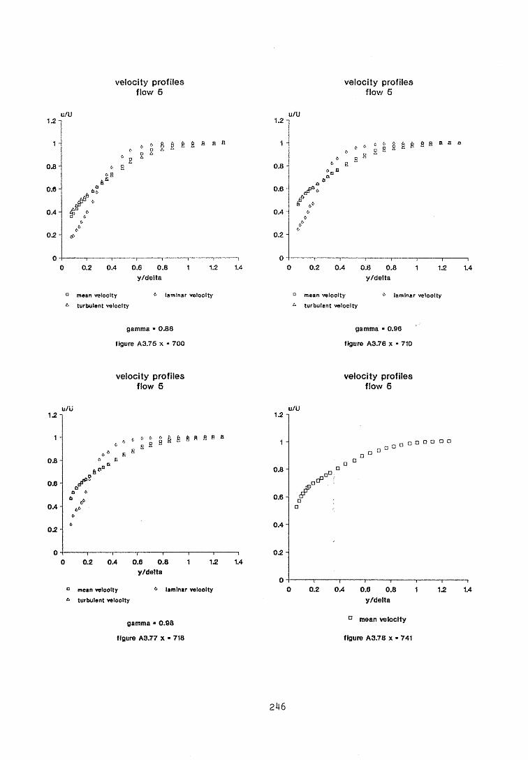
velocity profilesflow 6

u/u

° mean veloolty A turbulent velocity

* laminar velocity

velocity profilesflow 6

1.2

1 -

0.8 '

0.6

0.4

0.2

u/U

u

£ **

0.2 OA 0.8 0.8y/delta

1.2 1.4

a mean veloolty A turbulent velocity

laminar veloolty

gamma ■ 0.88 gamma - 0.96

figure A3.76 x « 700 figure A3.76 x ■ 710

velocity profiles flow 5

velocity profiles flow 6

u/U

c mean veloolty 6 laminar veloolty

A turbulent velocity

gamma - 0.98

figure A3.77 x - 718

u/U

D mean velocity

figure A3.78 x - 741

246

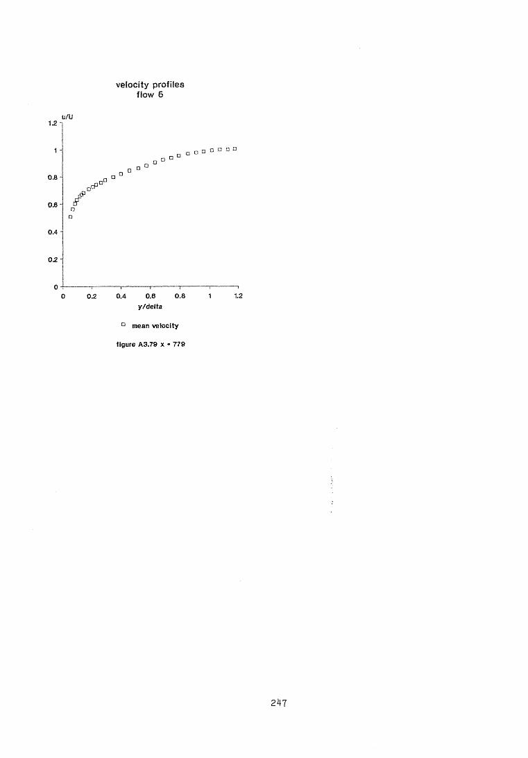
velocity profilesflow 6

u/U1.2 I

0 .8-1

0.6 aa

0.4 1

02 -

o o

00

—-----r-----1-----1----1 i0 2 0.4 0.8 0.8

y /delta

D mean velocity

figure A3.79 x « 779

o o a □

1.2

247

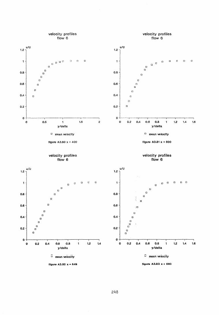
velocity profilesflow 6

velocity profilesflow 6

1-2 I

1 -

0.8

0.6 -

0.4

0.2 -

u/U

□ D □ O

00.5 1

y/delta

D mean velocity

figure A3.80 x - 400

1.5

1.2u/U

0.8

0.6

0.4

0.2 -

□ □ D C

0 ~l--- 1-- 1---- 1--- 1---1----1-- 1--- 10 0.2 0.4 0.6 0.8 1 13 1.4 1.6

y/delta

° mean velocity

figure A3.81 x • 600

velocity profiles flow 6

velocity profiles flow 6

1.2u/U

1 -

0.8

0 .6 -

0.4 -

0 3 -

a a o

—i----1----1---1---- 1---- 1---10.2 0.4 0.6 0.8 1 13 1.4

y/delta

u mean velocity

figure A3 .82 x ■ 6 4 Q

13u/U

Oil

0.6 -

0.4 -

0 3 -

□ □ D O

0 1--- 1--- 1--- 1--- 1--- 1----1--- 1-- 10 0 3 0 A 0.6 0.8 1 13 1.4 1.6

y/delta

E mean velocity

figure A3.B3 x ■ 56 0

2 4 8

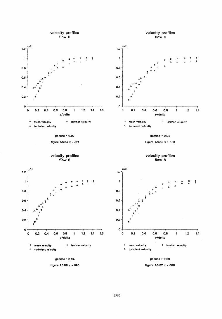
velocity profilesflow 6

velocity profilesflow 6

u/U

° mean veloolty & turbulent velocity

laminar velocity

1.2 -

1 -

0.8 -

0.6 -

0.4

0 2

u/U

00.2 0.4 0.6 0.8

y/delta

o o o& A tu

1 1.2 1.4

a mean veloolty A turbulent veloolty

* laminar velocity

gamma * 0.02

figure A3.84 x - 571

gamma - 0.03

figure A3.86 x - 580

velocity profiles flow 6

velocity profiles flow 6

u/U

° mean veloolty

& turbulent veloolty

* laminar velocity

1.2 -

1

0.8 -

0.6 -

0.4 -

02 -

u/U

a 4 ®4 4 •0-

o n e

i i i i i i0 0.2 0.4 0.6 0.8 1 1.2

y/delta

D mean velocity 6 laminar veloolty turbulent velocity

14

gamma * 0 0 4

figure A3.88 x • 590

gamma - 0.06

figure A3.87 x ■ 600

2 4 9

velocity profilesflow 6

velocity profilesflow 6

u/u

° mean velocity 6 laminar velocity& turbulent velocity'

U/U

D mean velocity * laminar velocity& turbulent veioolty

gamma « 0.11 gamma ■ 0.17

figure A3.88 x « 611 figure A3.89 x ■ 621

velocity profiles flow 6

velocity profiles flow 6

u/U u/U1 2 -] 1 2 ~

1 - a o 0 o o a

6 6 A A - * /-

fe A &

1 -

0.8 - 6 A

a

0.8 *

0.6- 0.6 -

0.4- d>too

0.4 -

0.2-

o -

too0

-------------1------------- 1------------- 1------------- 1------------- 1------------- 1------------- 1------------- 1

oo

k>

j---

------

-----

1—

0 0 2 0.4 0.6 0.8 1 12 1.4 1.6 0y/deita

a&□%c

v* 8a 6 • -

< * :

0.2

ab

0.4 0.8 0.8y/delta

6 0 OA * *

OA

1 12 1A

0 mean veioolty 0 laminar veloolty D mean veloolty o laminar veloolty& turbulent veioolty & turbulent veloolty

gamma - 0.24

figure A3.90 x ■ 629

gamma - 0.32

figure A3.91 x ■ 640

velocity profilesflow 6

velocity profilesflow 6

u /u u/U1 2 - 1 2 -

1 - ft s * “ 2 2 2 l

8 1 ‘ ‘

1 -

fta8 A A A

0 . 8 - 0 . 8 -

A &0 . 8 -

a a d

0 . 6 - . ^ 0

e ^ c PA o 0

A d o0 . 4 - D o

O 0 □ 0

0 . 4 - D 0

d D *a ft ft

0 . 2 -

o -

ftft

---------------1--------------- 1------------ ""1--------------- 1--------------- 1--------------- 1--------------- 3---------------1

0 2 -

o -

ftft

0.2 0.4 0.6 0.8 1 1.2 1.4 1.6y/delta

° mean veloolty & turbulent velocity

<■' laminar veloolty

& 6 0 c C g g

0 2 0.4 0.6 0.8 1 A2 1A 1.6y/delta

D mean veloolty A turbulent veloolty

* laminar velocity

gamma ■ 0.41

figure A3.B2 x - 650

gamma - 0.53

figure A3.93 x ■ 660

velocity profiles flow 6

velocity profiles flow 6

ifM u/U

D mean veloolty 0 laminar velocity

& turbulent veloolty

12 -i

1

0.8

0.8

0.4

0.2

0

,.6E'^ 'A □a d o a e a o

o o A 0 a ? Co A ^

0.2 0 A 0.6 0.8y/delta

12 1,4

° mean velocity

A turbulent veloolty

0 laminar veloolty

gamma - 0.63

figure A3.94 x ■ 669

gamma ■ 0.74

figure A3.86 x ■ 680

251

velocity profilesflow 6

velocity profilesflow 6

u/u

D mean velocity

A turbulent veloolty

laminar velocity

1.2 1

1

0.8 -

0.6 -

0.4

0 3.

U /U

0 a

ft 6 ft

6$

0.2 0.4 0.6 0.8y/delta

A g g& A

1.2 1.4

c mean velocity

A turbulent velocity

ft laminar veloolty

gamma • 0.83 gamma ■ 0.88

figure A3.96 x • 691 figure A3.97 x • 700

velocity profiles flow 6

velocity profiles flow 6

i i /«J u /U

n mean veloolty ft laminar veloolty ° mean veloolty 6 laminar velocity

A turbulent velocity A turbulent velocity

gamma ■ 0.94 gamma - 0.98

figure A3.98 x - 710 figure A3.99 x • 730

252

velocity profilesflow 6

velocity profilesflow 6

u/u

a mean velocity 0 laminar velocity

A turbulent velocity

1.2 U/U

0.8-

0.6- Z

n a D D ° ° D□ a D

0.4 -

02. ~

0 *1----1---- 1----1---- 1----1----i-----10 0.2 0.4 0.6 0.8 1 1.2 1.4

y/delta

gamma ■ 0.99 D mean velocity

figure A3.100 x « 749 figure A3.101 x - 770

velocity profiles flow 6

• •/lj

D mean velocity

figure A3.102 x • 780

253

velocity profilesflow 7

velocity profilesflow 7

1.2-1u /U

0 .8 -

0 .6 -

0.4-

0.2

□ □ □ □

0.6 1 1.6y/delta

D mean velocity

figure A3.103 x ■ 380

1.2 -i

1 -

0.8

0.8 -

0.4 -*

0.2-

u/U

□ □ d a

0 -)--t---1---- 1---1---1--- 1--1--- 1----10 0.2 0.4 0.6 0.8 1 1.2 1.4 1.6 1.8

y/delta

a mean velocity

figure A3.104 x ■ 460

velocity profiles flow 7

velocity profiles flow 7

u/U u/U

0 mean veioolty

turbulent velocity

o laminar velocity

1.2 -

1 -

0.8 -

0.8 -

S6r:

a* e :

0.4-

0.2 -

o - -------- 1---------p

Cs a a

n o a

0 0.2 0.4 0.6 0.8 1 1.2 1.4 1.6y/delta

D mean velocity

turbulent velocity

* laminar veioolty

gamma - 0.01

figure A3.105 x « 600

gamma * 0.02

figure A3.106 x • 660

2 5 4

velocity profilesflow 7

velocity profilesflow 7

u/U

° mean velocity

A turbulent velocity

laminar veloolty

gamma ■ 0.03

figure A3.107 x ■ 600

1-2 11 -

0 .8 -

0 .6 -

0.4

0.2

u/U

0

£s b o

AOAA 0

I?e

0.5

° mean veloolty

6 turbulent velocity

1 1.5y/delta

* laminar velocity

gamma - 0.07

figure A3.108 x - 650

velocity profiles flow 7

velocity profiles flow 7

u/U u/U

n mean veloolty 6 laminar velocity n mean velocity 0 laminar velocity

A turbulent veloolty A turbulent veloolty

gamma ■ 0.24 gamma - 0.68

figure A3.109 x ■ 700 figure A3.110 x • 750

255

velocity profilesflow 7

velocity profilesflow 7

1

0.8

0.6

0.4

0.2 i

1 2 .u/U uAJ

4, c- g fi 6n g & an a ^ g a s e

o S

o o

0.2 0.4 0.6 0.8 1 12 1.4y/delta

° mean veloolty

A turbulent velocity

o laminar velocity

12 -

1 -

0.8

0.8 -

0 A- 02 -

6 £ 0 6 0 C O A f e g g g f i f i„ s a H 8 * '

p - i--------------------1--------------------1-------------------- 1------------------ ,—

0 0.2 0.4 0.6 0.8 1 12y/delta

° mean velocity o laminar veloolty

A turbulent veloolty

1.4

gamma » 0.86

figure A3.111 x - 780

gamma ■ 0.97

figure A3.112 x ■ 850

velocity profiles flow 7

u/L!

° mean velocity

figure A3.113 x ■ 800

2 5 6

APPENDIX 4

DIGITAL PROCESSING OF HOT WIRE ANEMOMETER SIGNALS IN INTERMITTENTLY TURBULENT FLOWS

The published paper cited below has been removed from the e-thesis due to copyright restrictions:

Fraser, C.J., Graham, D. and Milne, J.S. (1990). Digital processing of hot wire anemometersignals in intermittently turbulent flows. In: Flow Measurement and Instrumentation, 1(4), pp.225-235.