boundary element method - arxiv
TRANSCRIPT
A residual a posteriori error estimate for the time–domain
boundary element method
Heiko Gimperlein∗† Ceyhun Ozdemir‡§ David Stark∗ Ernst P. Stephan‡
Abstract
This article investigates residual a posteriori error estimates and adaptive mesh re-finements for time-dependent boundary element methods for the wave equation. Weobtain reliable estimates for Dirichlet and acoustic boundary conditions which hold fora large class of discretizations. Efficiency of the error estimate is shown for a naturaldiscretization of low order. Numerical examples confirm the theoretical results. Theresulting adaptive mesh refinement procedures in 3d recover the adaptive convergencerates known for elliptic problems.
Mathematics Subject Classification: 65N38 (primary); 65M15; 35L67 (secondary)
Key words: boundary element method; a posteriori error estimates; adaptive mesh refine-ments; screen problems; wave equation.
1 Introduction
The efficient numerical treatment of boundary integral equations using adaptive mesh re-finement procedures has been extensively investigated for the numerical solution of homo-geneous elliptic problems in unbounded domains [11, 13]. See [27] for a recent exposition.
In this article we investigate the extension of the a posteriori error analysis and adap-tive mesh refinement procedures to initial-boundary value problems for the wave equation,formulated as boundary integral equations in the time-domain [17, 42]. We prove a reliablea posteriori error estimate of residual type for a large class of conforming discretizations.It is efficient for a time-domain boundary element method on a globally quasi-uniformmesh. The error estimate defines an adaptive mesh refinement procedure, which recoversthe convergence rates known for time-independent screen problems.
There has been recent interest in the solution of such problems on adapted meshes.Similar to the elliptic case, singularities of the solution may appear at singular points of theboundary, as discussed in [32, 33, 36], and in trapping regions. For finite element methods,
∗Maxwell Institute for Mathematical Sciences and Department of Mathematics, Heriot–Watt University,Edinburgh, EH14 4AS, United Kingdom, email: [email protected].†Institute for Mathematics, University of Paderborn, Warburger Str. 100, 33098 Paderborn, Germany.‡Institute of Applied Mathematics, Leibniz University Hannover, 30167 Hannover, Germany.§Institute for Mechanics, Graz University of Technology, 8010 Graz, Austria.
H. G. acknowledges partial support by ERC Advanced Grant HARG 268105 and the EPSRC Impact Accel-eration Account. C. O. was supported by a scholarship of the Avicenna Foundation.
1
arX
iv:2
008.
0429
7v1
[m
ath.
NA
] 1
0 A
ug 2
020

Muller and Schwab used the analytical results to recover quasi-optimal convergence rates ontime-independent graded meshes in 2d polygons. For boundary element methods in 3d time-independent graded meshes have been shown to recover quasi-optimal convergence rates foredge and corner singularities [22]. First steps towards time-adaptivity for singular temporalbehavior are due to Sauter and Veit [40] in 3 dimensions, and also convolution quadraturemethods with graded, non-adaptively chosen time steps have been studied, for example in[41]. Glafke [26] showed first results towards space-time refinements in 2 dimensions, and inunpublished work Abboud uses ZZ error indicators for computations with space-adaptivemesh refinements for screen problems.
The above works have shown the relevance of time-independent adapted meshes notonly in simple convex domains, but in realistic complex, heterogeneous geometries. For thenoise emission of car tires [7, 24] the sound amplification in the cuspidal, non-convex horngeometry between tire and road crucially determines the emitted sound. Time-independentmeshes graded into the horn are needed for the accurate computation of the sound emissioncharacteristics, due to the complexity of the geometry, even for a constant-coefficient PDE[22]. Adaptive meshes are expected to be of use in more general heterogeneous geometries,where the time-averaged indicators resolve persistent spatial inhomogeneities of the solu-tion such as in the current article. The error estimates presented in this article apply tomeshes locally refined in both space and time. In 2d, [26] uses such refinements to resolvespace-time singularities, such as travelling wave fronts, with space-time adaptive mesh re-finements. The approach requires to assemble n + 1 matrices in the n-th time step, anda feasible 3d implementation will require major algorithmic considerations in future work.In this article we focus on adaptive procedures for heterogeneous geometries, as a key steptowards general space-time singularities in 3d. It complements the work on adaptive time-stepping for a fixed spatial mesh by other authors [40].
To describe the main results, we consider the wave equation
∂2t u−∆u = 0 , u = 0 for t ≤ 0 ,
in the complement Rd \ Ω of a polyhedral domain or screen, with an emphasis on thechallenging case d = 3. On the boundary Γ = ∂Ω both Dirichlet and acoustic boundaryconditions,
u = f , respectively ∂νu− α∂tu = f ,
are considered. Here f is given, ν is the outer unit normal vector to Γ, and 0 < α,α−1 ∈L∞(Γ).
Following Bamberger and Ha Duong [5], we recast the boundary problem as a timedependent boundary integral equation. The Dirichlet problem is equivalent to a hyperbolicvariant of Symm’s integral equation:
Vφ(t, x) =
∫R+
∫ΓG(t− τ, x, y)φ(τ, y) dsy dτ = f(t, x) . (1)
Here φ is sought in a space-time anisotropic Sobolev space H1σ(R+, H−
12 (Γ)), and G is a
fundamental solution of the wave equation,
G(t− s, x, y) =H(t− s− |x− y|)
2π√
(t− s)2 + |x− y|2in 2d, (2)
G(t− s, x, y) =δ(t− s− |x− y|)
4π|x− y|in 3d. (3)
2

Here H is the Heaviside function and δ the Dirac distribution. Our results apply, in particu-lar, to a Galerkin discretization of the weak form of (1) in a subspace V ⊂ H1
σ(R+, H−12 (Γ)),∫
R+
∫ΓV∂tφ(t, x) ψ(t, x) dsx dσt =
∫R+
∫Γ∂tf(t, x) ψ(t, x) dsx dσt , (4)
dσt = e−2σtdt with σ > 0. For computations we consider subspaces V = V p,qh,∆t of tensor
products of piecewise polynomials in space and time, defined in Section 2. But also timediscretizations based on smooth functions are of interest [40].
This article shows that norms of the residual give upper and lower bounds for the error.The upper bound (5) holds for arbitrary discretizations, not only the Galerkin method (4),and for general meshes:
Theorem A: Let φ ∈ H1σ(R+, H−
12 (Γ)) be the solution to (4), and let φh,∆t ∈ H1
σ(R+, H−12 (Γ))
such that R = ∂tf − V∂tφh,∆t ∈ H0σ(R+, H1(Γ)). Then
‖φ− φh,∆t‖20,− 12,Γ,∗ .
∑i,∆
max(∆t)i, h∆ ‖R‖20,1,[ti,ti+1)×∆ . (5)
Let Γ be closed and polyhedral. For a globally quasi-uniform mesh on Γ, let V = W 0h,∆t
the tensor product of cubic splines in time with piecewise constant functions in space. Ifφh,∆t ∈ V is a Galerkin solution of (4) in V and φ ∈ H2
σ(R+, H−12 (Γ)), then for every
ε > 0max∆t, h‖R‖20,1−ε,Γ . ‖φ− φh,∆t‖22,− 1
2,Γ. (6)
The upper bound (5) is obtained in Corollary 4.5, the lower bound (6) in Theorems 5.1and 6.1. Our numerical results illustrate the a posteriori error estimate of Theorem A fortime-domain boundary elements based on (4).
Note the loss of time derivatives between the upper and lower bound of the error, inthe first Sobolev index. The loss is well-known for error estimates for hyperbolic problems[30], but see [44] for current work on a different inf-sup stable bilinear form. Our argumentsgeneralize to give reliable a posteriori estimates for the acoustic boundary problem, seeSection 3.2.
The residual error estimate from Theorem A is used to define adaptive mesh refinementsin space, based on the four steps Solve, Estimate, Mark, Refine. Numerical experimentsconfirm the efficiency and reliability of the estimate in examples. For screen problems,where the geometric singularities pose the greatest numerical challenges, they recover theconvergence rates known for elliptic problems.
Our analysis is in line with recent theoretical progress on time domain boundary ele-ment methods. Joly and Rodriguez [31] discuss practical Galerkin implementations withweight σ = 0, as opposed to theoretically justified weight functions. Aimi, Diligenti andcollaborators use formulations directly related to the conserved energy of the wave equationon a finite time interval [0,T) [1, 2, 3, 4]. At the expense of a slightly more involved weakformulation, the intrinsic coercivity implies the stability and convergence of these methods,rigorously proven for wave problems in a half-space. A detailed exposition of the mathe-matical background of time domain integral equations and their discretizations is available
3

in the monograph by Sayas [42], including methods based on convolution quadrature. See[17, 30] for more concise introductions.
This current work builds on the numerical analysis of adaptive boundary element meth-ods for the Laplace equation, both for Symm’s integral equation and the hypersingularequation [11, 13, 14, 15]. Work on different types of error indicators in the time-independentcase includes ZZ [12] and Faermann indicators [18, 19]. Our numerical examples for screensbuilds on the work by Becache and Ha Duong for crack problems in the time domain[8, 9, 29]. A comparison of different indicators in the time-domain will be the subject offuture research.
Structure of this article: Section 2 recalls the boundary integral operators associated to thewave equation as well as their mapping properties between suitable space-time anisotropicSobolev spaces. The Sobolev spaces are discretized using tensor products of piecewise poly-nomials in space and time. Section 3 presents a corresponding space-time discretization forthe formulation of the Dirichlet problem in terms of the single layer operator and derivesa reliable a posteriori error estimate in a simple setting, for globally quasi-uniform meshes,using a canonical approach which readily adapts to other settings. A second subsectionanalyzes an acoustic boundary problem, a system of equations involving in addition thedouble layer, adjoint double layer and hypersingular operators. Section 4 then localizes thespace-time Sobolev norm to derive the upper estimate for the Dirichlet problem for arbi-trary meshes in Theorem A. The upper estimates are complemented by a lower bound forthe error of a Galerkin approximation on globally quasi-uniform meshes in Section 5. Thefinal step of this proof is a lower bound for the best approximation in Section 6. Section7 discusses details of the implementation, and the algorithmic challenges towards efficientspace-time adaptive codes in 3d are outlined in Section 8. Section 9 finally presents numeri-cal experiments which confirm the theoretical results. An appendix shows relevant mappingproperties of the boundary integral operators for Sobolev exponents also outside the energyspace, Theorem 2.3.
Notation: We write f . g provided there exists a constant C such that f ≤ Cg. If theconstant C is allowed to depend on a parameter σ, we write f .σ g.
2 Preliminaries and discretization
In addition to the single layer operator V, for acoustic boundary problems we require itsnormal derivative K′, the double layer operator K and hypersingular operator W for x ∈ Γ,t > 0:
Kϕ(t, x) =
∫R+
∫Γ
∂G
∂ny(t− τ, x, y) ϕ(τ, y) dsy dτ , (7)
K′ϕ(t, x) =
∫R+
∫Γ
∂G
∂nx(t− τ, x, y) ϕ(τ, y) dsy dτ , (8)
Wϕ(t, x) = −∫R+
∫Γ
∂2G
∂nx∂ny(t− τ, x, y) ϕ(τ, y) dsy dτ . (9)
Space–time anisotropic Sobolev spaces on the boundary Γ provide a convenient settingto study the mapping properties of layer potentials. See [30, 23] for a detailed exposition.To define them, if ∂Γ 6= ∅, first extend Γ to a closed, orientable Lipschitz manifold Γ.
4

On Γ one defines the usual Sobolev spaces of supported distributions:
Hs(Γ) = u ∈ Hs(Γ) : supp u ⊂ Γ , s ∈ R .
Furthermore, Hs(Γ) is the quotient space Hs(Γ)/Hs(Γ \ Γ).To write down an explicit family of Sobolev norms, introduce a partition of unity αi subor-dinate to a covering of Γ by open sets Bi. For diffeomorphisms ϕi mapping each Bi into theunit cube ⊂ Rn, a family of Sobolev norms is induced from Rn, with parameter ω ∈ C\0:
||u||s,ω,Γ
=
(p∑i=1
∫Rn
(|ω|2 + |ξ|2)s|F
(αiu) ϕ−1i
(ξ)|2dξ
) 12
.
The norms for different ω ∈ C \ 0 are equivalent and F denotes the Fourier trans-form. They induce norms on Hs(Γ), ||u||s,ω,Γ = inf
v∈Hs(Γ\Γ)||u + v||
s,ω,Γand on Hs(Γ),
||u||s,ω,Γ,∗ = ||e+u||s,ω,Γ. We write Hsω(Γ) for Hs(Γ), respectively Hs
ω(Γ) for Hs(Γ), when a
norm with a specific ω is fixed. e+ extends the distribution u by 0 from Γ to Γ. As the norm||u||s,ω,Γ,∗ corresponds to extension by zero, while ||u||s,ω,Γ allows extension by an arbitraryv, ||u||s,ω,Γ,∗ is stronger than ||u||s,ω,Γ. Like in the time-independent case the norms are notequivalent whenever s ∈ 1
2 + Z [27].We now define a class of space-time anisotropic Sobolev spaces:
Definition 2.1. For σ > 0 and r, s ∈ R define
Hrσ(R+, Hs(Γ)) = u ∈ D′+(Hs(Γ)) : e−σtu ∈ S ′+(Hs(Γ)) and ||u||r,s,σ,Γ <∞ ,
Hrσ(R+, Hs(Γ)) = u ∈ D′+(Hs(Γ)) : e−σtu ∈ S ′+(Hs(Γ)) and ||u||r,s,σ,Γ,∗ <∞ .
D′+(E) respectively S ′+(E) denote the spaces of distributions, respectively tempered distri-butions, on R with support in [0,∞), taking values in a Hilbert space E. Here we considerE = Hs(Γ), respectively E = Hs(Γ). The relevant norms are given by
‖u‖r,s,σ := ‖u‖r,s,σ,Γ =
(∫ +∞+iσ
−∞+iσ|ω|2r ‖u(ω)‖2s,ω,Γ dω
) 12
,
‖u‖r,s,σ,∗ := ‖u‖r,s,σ,Γ,∗ =
(∫ +∞+iσ
−∞+iσ|ω|2r ‖u(ω)‖2s,ω,Γ,∗ dω
) 12
.
They are Hilbert spaces, and we note that the basic case r = s = 0 is the weightedL2-space with scalar product 〈u, v〉σ :=
∫∞0 e−2σt
∫Γ uvdsx dt. Because Γ is Lipschitz, like
in the case of standard Sobolev spaces these spaces are independent of the choice of αi andϕi when |s| ≤ 1.Using variational arguments, precise mapping properties are well-known for the layer po-tentials between Sobolev spaces related to the energy. Such estimates have been derived,for example, in [5, 6, 17, 28, 30], see [26] for the precise statement here.
Theorem 2.2. The following operators are continuous for r ∈ R:
V : Hr+1σ (R+, H−
12 (Γ))→ Hr
σ(R+, H12 (Γ)) ,
K′ : Hr+1σ (R+, H−
12 (Γ))→ Hr
σ(R+, H−12 (Γ)) ,
K : Hr+1σ (R+, H
12 (Γ))→ Hr
σ(R+, H12 (Γ)) ,
W : Hr+1σ (R+, H
12 (Γ))→ Hr
σ(R+, H−12 (Γ)) .
5

See also [31] for a detailed discussion of the mapping properties and [44] for an alternativescale of Sobolev spaces, in both references for Sobolev exponents related to the energy.In the appendix we extend classical arguments for the Laplace equation [16] to show thefollowing mapping properties also for exponents not related to the energy, as relevant tothis article:
Theorem 2.3. The following operators are continuous for r ∈ R, s ∈ (−12 ,
12):
V : Hr+1σ (R+, H−
12
+s(Γ))→ Hrσ(R+, H
12
+s(Γ)) ,
K′ : Hr+1σ (R+, H−
12
+s(Γ))→ Hrσ(R+, H−
12
+s(Γ)) ,
K : Hr+2σ (R+, H
12
+s(Γ))→ Hrσ(R+, H
12
+s(Γ)) ,
W : Hr+2σ (R+, H
12
+s(Γ))→ Hrσ(R+, H−
12
+s(Γ)) .
If Γ is C1,α for some α > 0, the operators are continuous for s ∈ [−12 ,
12 ].
For Lipschitz Γ, the end point estimate s = ±12 is known for elliptic problems, from
a deep result by Verchota [47]. Its extension to the wave equation is beyond the scope ofthis article and will be pursued elsewhere. When Ω = Rn+, Fourier methods yield improvedestimates for V and W:
Theorem 2.4 ([29], pp. 503-506). The following operators are continuous for r, s ∈ R:
V : Hr+ 1
2σ (R+, Hs(Γ))→ Hr
σ(R+, Hs+1(Γ)) ,
W : Hrσ(R+, Hs(Γ))→ Hr
σ(R+, Hs−1(Γ)) .
See also [31] for a recent discussion of mapping properties.
For simplicity, we assume that the hypersurface Γ consists of triangular faces Γi, Γ =∪Nsi=1Γi. Denote by hi the diameter of Γi, h = maxi hi. We choose a basis ϕpj of the spaceV ph of piecewise polynomial functions of degree p≥ 0 (continuous if p ≥ 1).
For the time discretization we consider a decomposition of the time interval R+ intosubintervals In = [tn−1, tn) with time step |In| = (∆t)n, n = 0, 1, . . . . Let ∆t = supn(∆t)n.We denote by βj,q a corresponding basis of the space V q
∆t of piecewise polynomial functionsof degree of q≥ 0 (continuous and vanishing at t = 0 if q ≥ 1). In addition to V q
∆t we alsorequire the space W∆t ⊂ V 3
∆t of cubic splines.The space-time cylinder R+ × Γ is discretized by local tensor products V p,q
h,∆t in space
and time. In the most general case R+×Γ =⋃i Si is a disjoint union of space-time elements
Si = [t1i , t2i )×Γi for some triangles Γi and time steps t1i , t
2i . We will call
⋃i Si shape regular
if there are constants c, c such that ch2i ≤ |Γi| ≤ ch2
i for all i. The discrete function spaceV p,qh,∆t consists of functions which restricted to Si are products of a polynomial of degreep ≥ 0 in space and a polynomial of degree q ≥ 0 in time, continuous in space if p ≥ 1 andcontinuous and vanishing at t = 0 if q ≥ 1.
We shall particularly focus on the case where the temporal mesh is the same for alltriangles, R+ × Γ =
⋃j,k[tj−1, tj) × Γjk, so that for all j,
⋃k Γjk is a triangulation of Γ. In
this case a basis for V p,qh,∆t is given by tensor products βj,q(t)ϕj,pk (x).
The space-time meshes generated by the adaptive mesh refinements considered beloware always a refinement of such a product mesh
⋃j,k[tj−1, tj) × Γjk, but not necessarily
6

themselves a product mesh. Here, we may consider the orthogonal projections Π∆t fromL2(R+) to V q
∆t, resp. Πh from L2(Γ) to V ph . See [23] for a discussion of their properties and
those of their composition Π∆tΠh. Furthermore, we define W ph,∆t = V p
h ⊗W∆t.
Note the following approximation properties for such meshes, see also Proposition 3.54of [26]:
Lemma 2.5. Let f ∈ Hrσ(R+, Hm(Γ)∩Hs(Γ)), 0 < m ≤ q+ 1, 0 < r ≤ p+ 1, s ≤ r, |l| ≤ 1
2such that ls ≥ 0. Then there exists fh,∆t = Π∆tΠhf such that for all l, s ≤ 0
‖f − fh,∆tf‖s,l,Γ ≤ C(hα + (∆t)β)||f ||r,m,Γ ,
where α = minm − l,m − m(l+s)m+r , β = minm + r − (l + s),m + r − m+r
m l. If l, s > 0,β = m+ r − (l + s).
3 A posteriori error estimates – reliability
3.1 Dirichlet problem
We recall the basic properties of the bilinear form
BD(φ, ψ) =
∫R+
∫ΓV∂tφ(t, x) ψ(t, x) dsx dσt
of the Dirichlet problem.
As shown in [30], the bilinear form is continuous, and also weakly coercive:
Proposition 3.1. For every φ, ψ ∈ H1σ(R+, H−
12 (Γ)) there holds:
|BD(φ, ψ)| . ‖φ‖1,− 12,Γ,∗‖ψ‖1,− 1
2,Γ,∗
and‖φ‖2
0,− 12,Γ,∗ . BD(φ, φ).
Note the loss of a time derivative between the upper and lower estimates. Alternativeinf-sup stable bilinear forms for the Dirichlet problem are the content of current work [44].
We consider a conforming Galerkin discretization of the Dirichlet problem (4) in a
subspace V ⊂ H1σ(R+, H−
12 (Γ)), which reads as follows: Find φh,∆t ∈ V such that
BD(φh,∆t, ψh,∆t) = 〈∂tf, ψh,∆t〉 , (10)
for all ψh,∆t ∈ V .
The well-posedness of the continuous and discretized problems are a basic consequenceof Proposition 3.1:
Corollary 3.2. Let f ∈ H2σ(R+, H
12 (Γ)). Then the Dirichlet problem (4) and its discretiza-
tion (10) admit unique solutions φ ∈ H1σ(R+, H−
12 (Γ)), φh,∆t ∈ V , and the estimates
‖φ‖1,− 12,Γ,∗, ‖φh,∆t‖1,− 1
2,Γ,∗ . ‖f‖2, 1
2,Γ
hold.
7
We note the Galerkin orthogonality:
BD(φ− φh,∆t, ψh,∆t) = 0 ∀ψh,∆t ∈ V .
Using ideas going back to Carstensen [11] and Carstensen and Stephan [13] for the bound-ary element method for elliptic problems, we obtain an a posteriori error estimate for theGalerkin solution to the Dirichlet problem on globally quasi-uniform meshes.
Theorem 3.3. Given V = V p,qh,∆t associated to a globally quasi-uniform discretization of
Γ, let φ ∈ H1σ(R+, H−
12 (Γ)), φh,∆t ∈ V the solutions to (4), resp. (10). Assume that
R = ∂tf − V∂tφh,∆t ∈ H0σ(R+, H1(Γ)). Then
‖φ− φh,∆t‖20,− 12,Γ,∗ . ‖R‖0,1,Γ
(∆t‖∂tR‖0,0,Γ + ‖h · ∇R‖0,0,Γ
). max∆t, h(‖∂tR‖20,0,Γ + ‖∇R‖20,0,Γ) .
Remark 3.4. The estimate generalizes to arbitrary subspaces V in place of V p,qh,∆t, in par-
ticular discretizations with smooth ansatz functions in time are of interest [40].a) With the endpoint estimate in Theorem 2.3, the single–layer potential maps H1
σ(R+, L2(Γ))continuously to H0
σ(R+, H1(Γ)), and Vφh,∆t belongs to H0σ(R+, H1(Γ)) if, for example,
φh,∆t ∈ H2σ(R+, L2(Γ)). The a posteriori estimate is therefore valid for discretizations
by piecewise constant functions in space and C1–continuous splines in time. In practice, asnoted in [31], the loss of time derivatives in the mapping properties of Theorems 2.2 and 2.3is not sharp, and R ∈ H0
σ(R+, H1(Γ)) can also be expected for lower-order discretizationsin time.b) In practice, we will here use ∆t‖∂tR‖0,0,Γ + ‖h · ∇R‖0,0,Γ as an error indicator.
Proof. We first note that for all ψh,∆t ∈ V p,qh,∆t
‖φ− φh,∆t‖20,− 12,Γ,∗ . BD(φ− φh,∆t, φ− φh,∆t)
=
∫R+
∫Γ∂tf(φ− φh,∆t) dsx dσt−BD(φh,∆t, φ− φh,∆t)
=
∫R+
∫Γ∂tf(φ− ψh,∆t) dsx dσt−BD(φh,∆t, φ− ψh,∆t)
=
∫R+
∫Γ(∂tf − V∂tφh,∆t)(φ− ψh,∆t) dsx dσt .
The last term may be estimated by:∫R+
∫Γ(∂tf − Vφh,∆t)(φ− ψh,∆t) dsx dσt ≤ ‖R‖0, 1
2,Γ‖φ− ψh,∆t‖0,− 1
2,Γ,∗ .
We use ψh,∆t = φh,∆t together with the interpolation inequality
‖R‖20, 1
2,Γ≤ ‖R‖0,0,Γ‖R‖0,1,Γ .
As the residual is perpendicular to V p,qh,∆t,
‖R‖20,0,Γ = 〈R,R〉 = 〈R,R− ψh,∆t〉 ≤ ‖R‖0,0,Γ‖R − ψh,∆t‖0,0,Γ
8

for all ψh,∆t ∈ V p,qh,∆t, we obtain
‖R‖0,0,Γ ≤ inf‖R − ψh,∆t‖0,0,Γ : ψh,∆t ∈ V p,qh,∆t .
Choosing ψh,∆t = Π∆tΠhR, based on the interpolation operator defined earlier, we obtain
‖R‖0,0,Γ . ∆t‖∂tR‖0,0,Γ + ‖h · ∇R‖0,0,Γ .
The theorem follows.
3.2 Acoustic boundary problems
Recall the wave equation with inhomogeneous acoustic boundary conditions
∂2t u−∆u = 0 on R+ × Rd \ Ω , ∂νu− α∂tu = f on R+ × Γ , u = 0 for t ≤ 0 .
For scattering problems f = −∂νuinc + α∂tuinc is determined from an incoming wave uinc.For a finite or infinite time interval [0, T ] we introduce the bilinear form
aT ((ϕ, p), (ψ, q)) =
∫ T
0
∫Γ
(αϕψ +
1
αpq +K′pψ −Wϕψ + V pq +Kϕq
)dsx dt . (11)
With
l(ψ, q) =
∫ T
0
∫ΓFψ dsx dt+
∫ T
0
∫Γ
Gq
αdsx dt , (12)
where F = −2∂νuinc, G = −2α∂tuinc, we consider the variational formulation for the waveequation in Rd with acoustic boundary conditions on Γ:
Find (ϕ, p) ∈ H1([0, T ], H12 (Γ))×H1([0, T ], L2(Γ)) such that
aT ((ϕ, p), (ψ, q)) = l(ψ, q) (13)
for all (ψ, q) ∈ H1([0, T ], H12 (Γ))×H1([0, T ], L2(Γ)).
Note that σ may be set to 0 in the definition of the Sobolev spaces when T <∞. Theacoustic problem is equivalent to the wave equation with acoustic boundary conditions [30].Its discretization reads:
Find (ϕh,∆t, ph,∆t) ∈ V p1,q1h,∆t × V
p2,q2h,∆t such that
aT ((ϕh,∆t, ph,∆t), (ψh,∆t, qh,∆t)) = l(ψh,∆t, qh,∆t) (14)
for all (ψh,∆t, qh,∆t) ∈ V p1,q1h,∆t × V
p2,q2h,∆t .
The following well-posedness holds:
Proposition 3.5. Let F ∈ H2([0, T ], H−12 (Γ)), G ∈ H1([0, T ], H0(Γ)). Then the weak
form (13) of the acoustic problem and its discretization (14) admit unique solutions (ϕ, p) ∈H1([0, T ], H
12 (Γ)) × H1([0, T ], L2(Γ)), resp. (ϕh,∆t, ph,∆t) ∈ V p1,q1
h,∆t × Vp2,q2h,∆t , which depend
continuously on the data.
9
We specifically note that the bilinear form aT satisfies a (weaker) coercivity estimate:
‖p‖20,0,Γ + ‖ϕ‖20,0,Γ . aT ((ϕ, p), (ϕ, p)) .
This follows from Equation (64) of [30],
aT ((ϕ, p), (ϕ, p)) = 2E(T ) +
∫ T
0
∫Γ
(α(∂tϕ)(∂tϕ) +
1
αp2
)dsx dt ,
where E(T ) = 12
∫Rd\Ω
(∂tu)2 + (∇u)2
dx is the total energy at time T .
We state a simple a posteriori estimate.
Theorem 3.6. Let (ϕ, p) ∈ H1([0, T ], H12 (Γ)) × H1([0, T ], L2(Γ)) be the solution to (13),
(ϕh,∆t, ph,∆t) ∈ V p1,q1h,∆t × V
p2,q2h,∆t the solution to the discretization (14). Assume that
R1 = F − αϕh,∆t + 2K′ph,∆t − 2Wϕh,∆t ∈ L2([0, T ], L2(Γ)) ,
R2 = G+ α−1ph,∆t + 2V ph,∆t − 2Kϕh,∆t ∈ L2([0, T ], L2(Γ)) .
Then
‖p− ph,∆t‖0,0,Γ + ‖ϕ− ϕh,∆t‖0,0,Γ . ‖R1‖0,0,Γ + ‖R2‖0,0,Γ .
Remark 3.7. From the mapping properties in Theorem 2.3, the assumptions are satisfiedif F,G ∈ L2([0, T ], L2(Γ)) and (ϕh,∆t, ph,∆t) ∈ H2([0, T ], H1(Γ)) × H1([0, T ], L2(Γ)). Forexample, this is true for discretizations with ϕh,∆t piecewise linear in space, higher-orderspline in time, and ph,∆t piecewise constant in space, piecewise linear in time. In practice,as noted in [31] for the single-layer potential, the loss of time derivatives in the mappingproperties of Theorems 2.2 and 2.3 is not sharp, and R1, R2 ∈ L2([0, T ], L2(Γ)) can also beexpected for lower-order discretizations in time.
Proof. For every (ψh,∆t, qh,∆t) ∈ V p1,q1h,∆t × V
p2,q2h,∆t we have
‖p− ph,∆t‖20,0,Γ + ‖ϕ− ϕh,∆t‖20,0,Γ. aT ((ϕ− ϕh,∆t, p− ph,∆t), (ϕ− ϕh,∆t, p− ph,∆t))= 〈R1, ϕ− ψh,∆t〉+ 〈R2, p− qh,∆t〉≤ ‖R1‖0,0,Γ‖ϕ− ψh,∆t‖0,0,Γ + ‖R2‖0,0,Γ‖p− qh,∆t‖0,0,Γ≤ (‖R1‖0,0,Γ + ‖R2‖0,0,Γ)(‖p− qh,∆t‖0,0,Γ + ‖ϕ− ψh,∆t‖0,0,Γ) .
The assertion is obtained by choosing (ψh,∆t, qh,∆t) = (ϕh,∆t, ph,∆t).
Naturally, for a quasi-uniform discretization of Γ and under stronger assumptions onR1, R2 we may obtain powers of h and ∆t on the right hand side by the following argument:
As in the proof of Theorem 3.3, 〈R1,˙ψh,∆t〉 = 〈R2, qh,∆t〉 = 0 for all (ψh,∆t, qh,∆t) ∈ V p1,q1
h,∆t ×V p2,q2h,∆t . Hence
‖R2‖20,0,Γ = 〈R2, R2〉 = 〈R2, R2 − qh,∆t〉 ≤ ‖R2‖0,0,Γ‖R2 − qh,∆t‖0,0,Γ.
10

Choosing qh,∆t = Π∆tΠhR2 yields
‖R2‖0,0,Γ . ∆t‖∂tR2‖0,0,Γ + ‖h · ∇ΓR2‖0,0,Γ + ∆t‖h · ∇Γ∂tR2‖0,0,Γ
provided R2 ∈ H1([0, T ], H1(Γ)).Assuming R1 ∈ H1([0, T ], H1(Γ)), we similarly have
‖R1‖20,0,Γ = 〈R1, R1〉 = 〈R1, R1 −˙ψh,∆t〉 ≤ ‖R1‖ 1
2−s,0,Γ‖
∫ t
0R1 − ψh,∆t‖ 1
2+s,0,Γ .
Choosing ψh,∆t = Π∆tΠh
∫ t0 R1 and s = 1
2 results as in Lemma 2.5 in
‖R1‖0,0,Γ . ∆t‖∂tR1‖0,0,Γ + ‖h · ∇ΓR1‖0,0,Γ + ∆t‖h · ∇Γ∂tR1‖0,0,Γ .
Altogether,
‖p− ph,∆t‖0,0,Γ + ‖ϕ− ϕh,∆t‖0,0,Γ + ‖ϕ− ϕh,∆t‖0, 12,Γ
. ‖R1‖0,0,Γ + ‖R2‖0,0,Γ
.2∑i=1
∆t‖∂tRi‖0,0,Γ + ‖h · ∇Ri‖0,0,Γ + ∆t‖h · ∇∂tRi‖0,0,Γ .
As in Remark 3.7, a sufficient condition for R1, R2 ∈ H1([0, T ], H1(Γ)) is given byF,G ∈ H1([0, T ], H1(Γ)) and (ϕh,∆t, ph,∆t) ∈ H3([0, T ], H2(Γ)) × H2([0, T ], H1(Γ)). Thisrequires an extension of Theorem 2.3 to Sobolev indices s > 1
2 , available for example usingpseudodifferential operator techniques for smooth Γ. Again, because Theorems 2.2 and 2.3are not sharp, less time regularity might be required in practice.
4 Error estimates for general discretizations
This section generalizes the results for the single layer potential without any assumptionson the underlying meshes.
We recall Lemma 3 in [22]:
Lemma 4.1. Let f1, . . . , fn ∈ Hrσ(R+, Hs(Γ)), 0 ≤ s ≤ 1, r ≥ 0, such that fjfk = 0 for
j 6= k. Let ωj be the interior of the support of fj with ωj = supp fj. Then
∥∥∥ n∑j=1
fj
∥∥∥2
r,s,Γ,∗≤ C
n∑j=1
‖fj‖2r,s,ωj ,∗ .
The constant C depends on Γ, but does not depend on fj or on n.
The lemma will be applied to a finite partition of unity Φ given by non-negative Lipschitzfunctions φjMj=1 on Γ such that
∑Mj=1 φj = 1.
Definition 4.2. The overlap of the partition of unity Φ is defined as K(Φ) = maxj cardk :φkφj 6= 0.
For a partition of unity associated to a triangulation, M tends to infinity as the meshsize decreases, while the overlap may be much smaller. We note a crucial observation from[14], Lemma 3.1:
11
Lemma 4.3. Let Φ be a finite partition of unity of Γ with overlap K(Φ). Then thereexists a partition of 1, . . . ,M into K ≤ K(Φ) non-empty subsets M1, . . . ,MK , such that⋃Kj=1Mj = 1, . . . ,M, Mj ∩Mk = ∅ if j 6= k and for all l ∈ 1, . . . ,K and j, k ∈Ml with
j 6= k, φjφk = 0 on [0, T ]× Γ.
Consider a space-time discretization R+×Γ =⋃l,j [tl−1, tl)×Γlj subordinate to product
mesh, and consider the partition of unity given by the associated hat functions φljj on Γ.On R+ we consider a partition of unity ψl∞l=0 such that ψl is supported in the interval
((l − 12)∆t, (l + 3
2)∆t), and therefore ψlψl′ = 0 whenever l ∈ M0 = 2N, l′ ∈ M1 = 2N + 1.
We obtain a partition of unity ψl,j = ψl ⊗ φljl,j on R+ × Γ.
Theorem 4.4. Let Γ′ ⊂ Γ be connected. and let Φ be a finite partition of unity with overlapK(Φ). Then for any f ∈ Hr
σ(R+, Hs(Γ′)) and any 0 ≤ s ≤ 1, we have
‖f‖2r,s,Γ′,∗ .σ K(Φ)∞∑l=0
M∑j=1
‖fψl,j‖2(1−s)r,0,Γ′ ‖fψl,j‖
2sr,1,Γ′ .
Proof. We show
‖f‖2r,s,Γ′,∗ . 2K(Φ)∞∑l=0
M∑j=1
‖fψl,j‖2r,s,Γ′,∗ . (15)
The assertion then follows from the interpolation estimate
‖fψl,j‖r,s,Γ′,∗ . ‖fψl,j‖1−sr,0,Γ′‖fψl,j‖sr,1,Γ′ .
To show (15), we consider a partitionM1, . . . ,MK as in Lemma 4.3. Then f =∑∞
l=0
∑Mj=1 ψl,jf ,
so that
‖f‖2r,s,Γ′,∗ = ‖1∑
m=0
∑l∈Mm
K∑k=1
∑j∈Mk
ψl,jf‖2r,s,Γ′,∗ ≤ 2K1∑
m=0
K∑k=1
‖∑l∈Mm
∑j∈Mk
ψl,jf‖2r,s,Γ′,∗ .
With Lemma 4.1 and Il = ((l − 1)∆t, (l + 2)∆t),
‖∑l∈Mm
∑j∈Mk
ψl,jf‖2r,s,Γ′,∗ ≤∑j∈Mk
‖∑l∈Mm
ψl,jf‖2r,s,ωj ,∗ ≤∑l∈Mm
∑j∈Mk
‖ψl,jf‖2r,s,Il×ωj ,∗ ,
so that
‖f‖2r,s,Γ′,∗ ≤ 2K
1∑m=0
∑l∈Mm
K∑k=1
∑j∈Mk
‖ψl,jf‖2r,s,Il×ωj ,∗ = 2K∞∑l=0
M∑j=1
‖ψl,jf‖2r,s,Il×ωj ,∗ ,
which shows (15).
Note the following Friedrichs inequality, which follows from the time-independent Friedrichsinequality and Fourier transformation into the time domain:
‖ψl,jf‖r,1,Γ′ .σ ‖∇(ψl,jf)‖r,0,Γ′ + ‖∂t(ψl,jf)‖r,0,Γ′ .
Therefore
‖ψl,jf‖2r,s,Il×ωj ,∗ . ‖ψl,jf‖2(1−s)r,0,Γ′ ‖ψl,jf‖
2sr,1,Γ′
.σ d2(1−s)j (1 + d2
j )s(‖∇(ψl,jf)‖2r,0,Γ′ + ‖∂t(ψl,jf)‖2r,0,Γ′
).
12

Here dj = maxδj ,∆t, where δj is the width of the support of φj , defined as the smallestnumber such that the following is true: There exists a direction n ∈ R3, |n| = 1, suchthat for all x ∈ R3 and for each plane H perpendicular to n with x ∈ H, the intersectionsupp φj ∩H is a Lipschitz curve of length ≤ δj .
We now use V∂t(φ− φh,∆t) = R, the coercivity of V∂t in Proposition 3.1, and Theorem4.4 with s = 1
2 . We obtain the following a posteriori error estimate, with the residuallocalized in the space-time elements:
Corollary 4.5. Let φ ∈ H1σ(R+, H−
12 (Γ)) be the solution to (4), and let φh,∆t ∈ H1
σ(R+, H−12 (Γ))
such that R = ∂tf − V∂tφh,∆t ∈ H0σ(R+, H1(Γ)). Then with l,j = supp ψl,j,
‖φ−φh,∆t‖20,− 12,Γ,∗ .σ
∑l,j
dj
(‖∇R‖20,0,l,j + ‖∂tR‖20,0,l,j
)'∑l,j
max(∆t)l, hl,j ‖R‖20,1,l,j .
5 Lower bounds
As for time-independent problems, for the discussion of lower bounds we restrict ourselvesto globally quasi-uniform meshes on a polyhedral screen Γ.
Because of the different norms in the upper and lower bounds for BD in Proposition3.1, the a posteriori estimate only satisfies a weak variant of efficiency:Provided φ ∈ H2
σ(R+, H0(Γ)) from the mapping properties of V in Theorem 2.3 we concludefor ε ∈ (0, 1):
max∆t, h−1−ε
2 ‖φ− φh,∆t‖0,− 12,Γ,∗ .
‖R‖0,1−ε,Γ = ‖V(∂tφ− ∂tφh,∆t)‖0,1−ε,Γ . ‖φ− φh,∆t‖2,−ε,Γ ≤ ‖φ− φh,∆t‖2,0,Γ .
A proof of the sharp estimate, ε = 0, follows from the endpoint estimate s = 12 in Theorem
2.3. As mentioned there, it is known for Γ of class C1,α and, for elliptic problems, from adeep result by Verchota for Lipschitz Γ.
As in the elliptic case, we aim to use the mapping properties of V together with approx-imation properties of the finite element spaces to recover the same spatial Sobolev index−1
2 in the upper and lower estimates.
Theorem 5.1. Assume that R= ∂tf − V∂tφh,∆t ∈ H0σ(R+, H1(Γ)) and that the ansatz
functions V = W ph,∆t ⊂ H
2σ(R+, H0(Γ)) ∩ V p,q
h,∆t satisfy
infψh∆t∈V
‖φ− ψh∆t‖2,0,Γ ' maxh,∆tβ (16)
for some β > 0. Then for all ε ∈ (0, 1)
‖R‖0,1−ε,Γ .maxh−12 , (∆t)−
12 ‖φ− φh∆t‖2,− 1
2,Γ.
Remark 5.2. In Theorem 6.1 below, the hypothesis (16) is verified using the singularexpansion of the solution φ at the edges and corners.
For the proof, we require an auxiliary projection Ph,∆t from H2(R+, H−1(Γ)) into thespace of ansatz functions ⊆ H2(R+, L2(Γ)) such that Ph,∆t is H2(R+, L2(Γ))-stable.
13

For the construction of Ph,∆t = P∆tQ∗h we use a projection P∆t on the space of cubicsplines W∆t ⊂ V 3
∆t in time and a Galerkin projection Q∗h in space.More precisely, we consider the projection Qh : L2(Γ) → V p
h defined as follows: Forφ ∈ L2(Γ), we let Qhφ ∈ V p
h be the unique solution to the variational problem
〈Qhφ, ψh〉 = 〈φ, ψh〉
for all ψh ∈ V ph . Qh is bounded on L2(Γ) and self-adjoint, Qh = Q∗h. Therefore, if Qh
restricts to a bounded operator on Hsω(Γ), Qh = Q∗h extends with the same norm to a
bounded operator on H−sω (Γ).For triangulations on which Qh is a bounded operator on H1(Γ), we show that the
operator norm is uniformly bounded in ω:
Lemma 5.3. Let s ∈ [0, 1] and Qh bounded on H1(Γ). Then for all φ ∈ Hsω(Γ), we have:
‖Qhφ‖s,ω,Γ ≤ C‖φ‖s,ω,Γ.
For all φ ∈ H−sω (Γ), we have:
‖Qhφ‖−s,ω,Γ,∗ ≤ C‖φ‖−s,ω,Γ,∗.
The conditions are satisfied, for example, on quasi-uniform meshes [10], or more generallyon adaptive meshes generated by NVB refinements. We only use it in the quasi-uniformcase.
Proof. For the first assertion we note that it is clear for s = 0. We show it for s = 1, andthe case for general s ∈ [0, 1] follows from interpolation.
By assumption,‖∇Qhφ‖L2(Γ) ≤ C‖φ‖H1(Γ).
Further Qh is bounded with norm 1 on L2(Γ), so that
‖Qhφ‖L2(Γ) ≤ ‖φ‖L2(Γ) .
With‖Qhφ‖21,ω,Γ = ‖ωQhφ‖2L2(Γ) + ‖∇Qhφ‖2L2(Γ),
we conclude‖Qhφ‖21,ω,Γ ≤ ‖ωφ‖2L2(Γ) + C2‖φ‖2H1(Γ) ≤ C
2‖φ‖21,ω,Γ .
This shows the first assertion for s = 1.The second assertion follows from the first one, with the same constant C. Indeed,
‖Qhφ‖−s,ω,Γ,∗ = sup0 6=ψ∈Hs
ω(Γ)
〈Qhφ, ψ〉L2(Γ)
‖ψ‖s,ω,Γ= sup
06=ψ∈Hsω(Γ)
〈φ,Qhψ〉L2(Γ)
‖ψ‖s,ω,Γ≤ C‖φ‖−s,ω,Γ,∗ .
Using the Laplace transform to transfer the result into the time-domain, we obtain
‖Qhφ‖r,−s,Γ,∗ ≤ C‖φ‖r,−s,Γ,∗
for s ∈ [0, 1] and all r. Further note that the interpolation operator P∆t in time for cubicsplines is continuous on H2 functions. The continuity extends to H2(R+, H−s(Γ)). Weconclude:
14

Lemma 5.4. Consider a quasi-uniform mesh, s ∈ [0, 1] and Ph,∆t = P∆tQh. For all
φ ∈ H2(R+, H−s(Γ)), we have
‖Ph,∆tφ‖2,−s,Γ,∗ ≤ C‖φ‖2,−s,Γ,∗.
The approximation properties of Ph,∆t analogous to Lemma 2.5 follow as in [26], Propo-sition 3.54.
Proof of Theorem 5.1. The theorem partly follows the functional analytic approach of [11]for the time-independent case. We consider the following quantities: the error of the bestapproximation Πh,∆tφ of φ in H2
σ(R+, L2(Γ)),
E(φ, h,∆t) = ‖φ−Πh,∆tφ‖2,0,Γ ,
where E(φ, h,∆t) ' maxh,∆tβ by (16); the relative error of best approximation,
F (φ, h,∆t) =‖φ−Πh,∆tφ‖2,−1,Γ
‖φ−Πh,∆tφ‖2,0,Γ;
and the inverse inequality [26]
G(h,∆t) = supψh∆t 6=0
‖ψh,∆t‖2,0,Γ‖ψh,∆t‖2,−1,Γ
. maxh−1,∆t−1.
Their analysis relies on the projection operator Ph,∆t from Lemma 5.4.Note that F (φ, h,∆t) . maxh,∆t. Indeed because φ ∈ H2
σ(R+, H0(Γ)), by dualityand the approximation properties of Πh,∆t:
‖φ−Πh,∆tφ‖2,−1,Γ = supη
〈φ−Πh,∆tφ, η −Πh,∆tη〉‖η‖−2,1,Γ
. maxh,∆t‖φ−Πh,∆tφ‖2,0,Γ.
This uses the estimate ‖η −Πh,∆tη‖−2,0,Γ . maxh,∆t‖η‖−2,1,Γ.From the beginning of this section, we recall
‖R‖0,1−ε,Γ . ‖φ− φh,∆t‖2,0,Γ ≤ ‖φ−ΠH,∆Tφ‖2,0,Γ + ‖ΠH,∆Tφ− φh,∆t‖2,0,Γ .
Note that the first term is ‖φ − ΠH,∆Tφ‖2,0,Γ = E(φ,H,∆T ). For the second term weobserve that
‖ΠH,∆Tφ− φh,∆t‖2,0,Γ . G(H,∆T )‖ΠH,∆Tφ− φh,∆t‖2,−1,Γ ,
so that ‖ΠH,∆Tφ− φh,∆t‖2,0,Γ . G(H,∆T )1/2‖ΠH,∆Tφ− φh,∆t‖2,− 12,Γ. We conclude
‖R‖0,1−ε,Γ . E(φ,H,∆T ) +G(H,∆T )1/2‖ΠH,∆Tφ− φh,∆t‖2,− 12,Γ .
Further,
‖ΠH,∆Tφ− φh,∆t‖2,− 12,Γ ≤ ‖ΠH,∆Tφ− φ‖2,− 1
2,Γ + ‖φ− φh,∆t‖2,− 1
2,Γ .
From the definition of F and interpolation, ‖ΠH,∆Tφ− φ‖2,− 12,Γ is bounded by
. F (φ,H,∆T )1/2‖ΠH,∆Tφ− φ‖2,0,Γ = F (φ,H,∆T )1/2E(φ,H,∆T ) .
15

To sum up,
‖φ− φh,∆t‖2,0,Γ . E(φ,H,∆T ) +G(H,∆T )1/2F (φ,H,∆T )1/2E(φ, h,∆t)
+G(H,∆T )1/2‖φ− φh,∆t‖2,− 12,Γ
≤ E(φ,H,∆T )
E(φ, h,∆t)‖φ− φh,∆t‖2,0,Γ(1 +G(H,∆T )1/2F (φ,H,∆T )1/2)
+G(H,∆T )1/2‖φ− φh,∆t‖2,− 12,Γ ,
or, with δ = E(φ,H,∆T )E(φ,h,∆t) (1 + F (φ,H,∆T )1/2G(φ,H,∆T )1/2) and a constant C,
‖φ− φh,∆t‖2,0,Γ .G(H,∆T )1/2
1− Cδ‖φ− φh,∆t‖2,− 1
2,Γ .
If δ = E(φ,H,∆T )E(φ,h,∆t) (1 + F (φ,H,∆T )1/2G(φ,H,∆T )1/2) < 1
2C , we obtain
‖R‖0,1−ε,Γ . G(H,∆T )1/2‖φ− φh∆t‖2,− 12,Γ .
Here H and ∆T are sufficiently small compared to h and ∆t, and it remains to choose themso that δ < 1
2C . Set H = ρh and ∆T = ρ∆t for ρ ∈ (0, 1). Using that
F (φ, ρh, ρ∆t)G(φ, ρh, ρ∆t) ' maxh,∆tminh,∆t
is uniformly bounded in ρ ∈ (0, 1), so that it suffices to show that E(φ,ρh,ρ∆t)E(φ,h,∆t) → 0 as ρ tends
to 0. This follows from (16).
6 Best approximation and lower bounds
In this section we verify the hypothesis (16) in Theorem 5.1 for polyhedral domains, byproving upper and lower bounds for the best approximation of the solution to the waveequation with Dirichlet boundary conditions.
Let Ω be a polyhedral domain and u a solution to the wave equation in Ω:
∂2t u(t, x)−∆u(t, x) = 0 in R+
t × Ωx , (17)
u(t, x) = g(t, x) on Γ = ∂Ω , (18)
u(0, x) = ∂tu(0, x) = 0 in Ω. (19)
The function u exhibits well-known singularities at non-smooth boundary points of thedomain. Locally near an edge or a corner, Ω is of the form R+×K, where the base K ⊂ S2
is a smooth or polygonal subset of the sphere. The solution may be decomposed into aleading part given by explicit singular functions plus less singular terms [25, 32, 33, 36]. Werefer to [32, Theorem 7.4 and Remark 7.5] for details in the case of the Neumann problemin a wedge, respectively [33, Theorem 4.1] for the Dirichlet problem in a cone and state thedecomposition in terms of polar coordinates (r, θ) centered at the vertex (0, 0, 0):
u(t, x) = u0(t, r, θ) + χ(r)rλa(t, θ) + χ(θ)b1(t, r)(sin(θ))ν
+ χ(π2 − θ)b2(t, r)(cos(θ))ν , (20)
∂nu(t, x) = ψ0(t, r, θ) + χ(r)rλ−1a(t, θ) + χ(θ)b1(t, r)r−1(sin(θ))−ν
+ χ(π2 − θ)b2(t, r)r−1(cos(θ))−ν . (21)
16

Here, ν = πα , where α is the opening angle of the wedge, and λ = −1
2 +√
14 + µ, where µ is
the smallest eigenvalue of the Laplace-Beltrami operator with Dirichlet boundary conditionsin the subdomain K of the sphere. χ, χ are cut-off functions and a, bj sufficiently regular.For generic problems the functions a, b1, b2 are not identically zero.
From the representation formula, the wave equation translates into the boundary integralequation V φ = f , with f = (1−K)g and solution φ = ∂nu|Γ.
The main theorem concerning the approximation of φ is:
Theorem 6.1. Assume that the coefficient functions a, b1, b2 are not identically 0. ThenE(φ, h,∆t) ' maxh,∆tmaxν− 1
2,λ.
In particular, hypothesis (16) is satisfied. A similar result in the elliptic case was knownif Γ is a curve, i.e. in dimension 2 [11].
The key step in the proof of Theorem 6.1 is to show the result for bilinear basis functionson a rectangular mesh. For simplicity of notation, we restrict to one boundary face of Γ andassume it is given by Q × 0 with corner of the domain at (0, 0, 0), where Q = (0, 1)2 =⋃klQkl, Qkl = [xk−1, xk)× [xl−1, xl) and xk = kh.
Recall the following estimate from [22]:
Lemma 6.2. Let −1 ≤ s ≤ 0, 0 ≤ r ≤ ρ ≤ p+ 1, Q = [0, h1]×[0, h2], u ∈ Hρσ([0,∆t], H1(R)),
Πptu the orthogonal projection onto piecewise polynomials in t of order p, and Π0
x,y the or-
thogonal projection onto piecewise constant polynomials in space, Π0x,yu = 1
h1h2
∫Q
u(t, x, y)dy dx.
Then for U = ΠptΠ
0x,yu we have
‖u− U‖r,s,Q,∗ . (∆t)ρ−rmaxh1, h2,∆t−s‖∂ρt u‖L2([0,∆t]×Q) (22)
+ maxh1, h2,∆t−s(h1‖ux‖L2([0,∆t]×Q) + h2‖uy‖L2([0,∆t]×Q)
).
If u(t, x, y) = u1(t, x)u2(y), u1 ∈ Hρσ([0,∆t], H1([0, h1])), u2 ∈ H1([0, h2]) then
‖u− U‖r,s,Q,∗ . (∆t)ρ−rmaxh1,∆t−s‖∂ρt u‖L2([0,∆t]×Q)
+(h1−s
1 ‖ux‖L2([0,∆t]×Q) + h1−s2 ‖uy‖L2([0,∆t]×Q)
).
Proof of Theorem 6.1. We use the upper bound E(φ, h,∆t) . maxh,∆tmaxν− 12,λ and
first approximate the corner singularity f = rλ−1a(t, θ), a ∈ Hρσ(R+, H1([0, π/2])). With
p|Qkl = ΠptΠ
0x,yf and Lemma 6.2 one obtains
‖f − p‖20,0,Q .N∑
k,l=1k+l 6=2
((∆t)2ρ‖∂ρt f‖20,0,Qkl + h2
k‖fx‖20,0,Qkl + h2l ‖fy‖20,0,Qkl
)+ ‖f − p‖20,0,Q11
. (23)
For k > 2, l > 2 the following estimate holds, with the zeta function ζ(s):
N∑k,l=2
h2k‖fx‖20,0,Qkl =
N∑k=2
h2k
∫ ∞0
∫ π/2
φ=0w(t, θ)2dθ dσt
∫ √2(k+1)h
√2kh
r2λ−4rdr
.∞∑k=2
h2λk2λ−3 = ch2λζ(3− 2λ) .
17

Here we have used|fx(t, x, y)| 6 rλ−2w(t, θ)
with w ∈ Hρσ(R+, H0([0, π/2])).
For k = 1, l > 1 (and analogously for k > 1, l = 1), in (23) we compute that
N∑l=2
h21‖fx‖20,0,Q1l
6 h21
∫ ∞0
h1∫x=0
1∫y=0
|fx(t, x, y)|2dy dx dσt
6 h21
∫ ∞0
√2∫
r=h
π/2∫φ=0
a2(t, θ)dθ r2λ−3dr dσt
. h21 + h2λ
1 .
Finally, in the corner k = 1, l = 1 the singular function f ∈ Hρσ(R+, H0(Q11)), because
λ > 0. Now‖f − p‖0,0,Q11 . ‖f‖0,0,Q11 ' hλ1 .
We now consider the approximation of the edge singularities, which are of two types,fixing Q = [0, 1]2 with singularity at the x-axis:
(i) f(t, x, y) = χ(x)b(t, x)yν−1 with edge intensity factor b ∈ Hρσ(R+, H1
0 (R+)),
(ii) f(t, x, y) = χ(x)b(t)xλ−νyν−1 with a corner singularity in the edge intensity factor.
We have
‖f − p‖20,0,Q .N∑
k,l=1
‖f − p‖20,0,Qkl . (24)
First consider case (ii), where the time dependence factors out. Define
p2 =1
h2
∫I∗j−1
f2(y)dy, p1 =1
h1
∫Ij
f1(x)dx, f2(y) = yν−1, f1 = xλ−ν ,
where h = h1 = h2, Ij = [xj−1, xj ] and I∗k = [0, xk]. Then one computes
‖f2 − p2‖2L2(0,h) =(ν − 1)2
(1 + (ν − 1)2)(2(ν − 1) + 1)h2(ν−1)+1
‖f2 − p2‖2L2(a,a+h) = a2(ν−1)+1η(ha ), a > 0, where
η(δ) =(1 + δ)2(ν−1)+1 − 1
2(ν − 1) + 1− [(1 + δ)(ν−1) − 1]2
δ(1 + (ν − 1))2
and δ > 0. With Q∗j = ∪j−1l=1Qjl = Ij × I∗j−1, one notes
‖f2 − p2‖2L2(I∗j−1)‖p1‖2L2(Ij)= h2(ν−1)+1
[ (ν − 1)2
(1 + (ν − 1)2)(2(ν − 1) + 1)+
j−1∑l=1
(xlh )2(ν−1)+1η(h2xl
)] ∫ xj
xj−1
1
h21
(∫ xj
xj−1
xλ−νdx
)2
dx
18

and ∫ xj
xj−1
1
h21
(∫ xj
xj−1
xλ−νdx
)2
dx = x2λ−2ν+1j−1
xj−1
h
[(1 + hxj−1
)λ−ν+1 − 1]2
(λ− ν + 1)2.
As η( hxl ) .h3
x3l
and
1
δ
[(1 + δ)λ−ν+1 − 1]2
(λ− ν + 1)2=
1
δ
[(λ− ν + 1)δ + (λ− ν + 1)(λ− ν)δ2 +O(δ3)]
(λ− ν + 1)2
= δ + (λ− ν + 1)δ2 +O(δ3) ,
we obtain
N∑j=2
‖f2 − p2‖2L2(I∗j−1)‖p1‖2L2(Ij)=
N∑j=2
h2(ν−1)+1[(ν − 1)2
(1 + (ν − 1)2)(2(ν − 1) + 1)
+
j−1∑l=1
(xlh )2(ν−1)−2][(j − 1)h]2λ−2ν+1(j − 1)[(1 + 1
j−1)λ−ν+1 − 1]2
(λ− ν + 1)2.
The estimate
N∑j=2
‖f2 − p2‖2L2(I∗j−1)‖p1‖2L2(Ij)= c
N∑j=2
h2(ν−1)+1(j − 1)2λ−2νh2λ−2ν+1
= h2(ν−1)+1h2λ−2ν+1N−1∑k=1
k2λ−2ν . ζ(2ν − 2λ)h2λ
follows and may be integrated in time.Now consider
‖f1 − p1‖2L2(Ij)= ‖xλ−ν − 1
h
∫Ijxλ−νdx‖2L2(Ij)
=
a2(λ−ν)+1η(ha ), a > 0
(λ−ν)(1+(λ−ν)2)(2(λ−ν)+1)
h2(λ−ν)+1, a = 0 .
For j ≥ 2
‖f1 − p1‖2L2(Ij)=
x2(λ−ν)+1j
h2(λ−ν)+1 η(hxj
)h2(λ−ν)+1 = (
xjh )2(λ−ν)−2h2(λ−ν)+1,
‖f2‖2L2(I∗j−1) =
∫ xj−1
0y2ν−2dy . x2ν−1
j−1 ,
and
‖f1 − p1‖2L2(Ij)‖p2‖2L2(I∗j−1) = (
xjh )2(λ−ν)−2(
xj−1
h )2ν−1h2(λ−ν)+1h2ν−1
6 (xjh )2(λ−ν)−2+2ν−1h2(λ−ν)+1+2ν−1.
We have
N∑j=2
‖f1 − p1‖2L2(Ij)‖f2‖2L2(I∗j−1) = c
∞∑j=1
j2(λ−ν)−2+2ν−1h2λ−2ν+1+2ν−1 = cζ(3− 2λ)h2λ .
19
Again, this estimate may be integrated in time.We now consider case (i): f(t, x, y) = b(t, x)yν−1 +(χ(x)−1)b(t, x)yν−1 =: f1 +f2 for ν > 1
2and Q = [0, 1]2 = I × I, with I = [0, 1]. Again we define
q1 = Πpt
∫ 1
0b(t, x)dx, q2 =
∫ 1
0yν−1dy .
Note that with f2(t, x, y) = (χ(x)− 1)b(t, x)yν−1 ∈ H0σ(R+, H1(Q)) we get
‖f2 − q1q2‖20,0,Q . h2 .
Since
‖yν−1 − q2‖2L2(I) ' h2ν−1, ‖yν−1‖2L2(I) ≤ c
and‖b− q1‖20,0,I . maxh,∆t2
(‖∂tb‖20,0,I + ‖∂xb‖20,0,I
),
we have
‖b(t, x)yν−1 − q1(t, x)q2(y)‖20,0,Q. ‖b‖20,0,I‖yν−1 − q2‖2L2(I) + ‖yν−1‖2L2(I)‖b− q1‖20,0,I . h2ν−1 + maxh,∆t2 . (25)
For the lower bound, we first consider the error in Q11 resulting from the corner singu-larity. There the error of approximation by a spatially constant function c is given by
‖a(t, θ)rλ−1 − c(t)‖20,0,Q11&∫ ∞
0
∫ h
0
∫ π/2
0r(a(t, θ)rλ−1 − c)2dθ dr dσt .
If a 6= 0, we may find a small intervall (θ0 − δ, θ0 + δ) on which a is nonzero for a timeinterval I. We estimate
‖a(t, θ)rλ−1 − c‖20,0,Q11&∫I
∫ h
0
∫ θ0+δ
θ0−δr(a(t, θ)rλ−1 − c)2dθ dr dσt .
As a is a restriction of an eigenfunction of the Laplace-Beltrami operator, it is smooth, andup to higher order terms (h.o.t.) in h we compute∫
I
∫ h
0
∫ θ0+δ
θ0−δr(a(t, θ)rλ−1 − c)2dθ dr dσt
=
∫I
∫ h
0
∫ θ0+δ
θ0−δr(a(t, θ0)rλ−1 − c)2dθ dr dσt+ h.o.t.
= 2δ
∫I
∫ h
0r(a(t, θ0)rλ−1 − c)2dr dσt+ h.o.t.
Now we may explicitly compute the infimum over c:∫I
∫ h
0r(a(t, θ0)rλ−1 − c)2dr ≥ Cσ|I|min
t∈Ia(t, θ0)2 (λ− 1)2
2λ(λ+ 1)2h2λ .
This lower order bound for the error of order hλ matches with the upper bound from above.
20
An analogous argument for the regular edge intensity factor, case (i), shows that theinequality (25) is an equality up to higher order terms in h. We therefore obtain
‖b(x)yν−1 − q1(x)q2(y)‖0,0,Q & hν−12 + h.o.t.
In a neighborhood of the edge or corner, the solution is given by its singular expansion, andthe approximation error coincides with the approximation error for the singular functions,b(t, x)yν−1, yλ−νi ρν−1, respectively a(t, θ)rλ−1, up to lower order terms in h. We concludethat
E(φ, h,∆) = ‖φ−Πh,∆tφ‖2,0,Γ & maxh,∆tminν− 12,λ + h.o.t. .
References [37, 38] show how to deduce approximation results for piecewise linear functionson triangular meshes from piecewise bilinear functions on rectangles. Altogether, the proofof Theorem 6.1 is complete.
7 Algorithmic details
The a posteriori error estimate from Theorem A leads to an adaptive mesh refinementprocedure, based on the four steps:
SOLVE −→ ESTIMATE −→MARK −→ REFINE.
The precise algorithm is given as follows:
Adaptive Algorithm:Input: Spatial mesh T = T0, refinement parameter θ ∈ (0, 1), tolerance ε > 0, data f .
1. Solve Vϕh,∆t = f on T .
2. Compute the error indicators η(4) in each triangle 4 ∈ T .
3. Find ηmax = max4 η(4).
4. Stop if∑
i η2(Mi) < ε2.
5. Mark all 4 ∈ T with η(Mi) > θηmax.
6. Refine each marked triangle into 4 new triangles to obtain a new mesh TChoose ∆t such that ∆t
∆x ≤ 1 for all triangles.
7. Go to 1.
Output: Approximation of ϕ.
In the first step, we solve V ϕ = f using the Galerkin discretization (10) in V 1,1h,∆t. The
Galerkin solution has the form
ϕh,∆t(x, t) =
Nt∑m=1
Ns∑i=1
ϕmi βm(t)ξi(x) ,
where βm is the piecewise linear hat function in time associated to time tm,
βm(t) = (∆t)−1((t− tm)χ[tm−1,tm](t)− (t− tm+1)χ[tm,tm+1](t)),
21
and ξi is the piecewise linear hat function in space associated to node i.As a step towards adaptive mesh refinements in space-time, we here focus on time-
integrated error indicators as they are relevant for geometric singularities. As shown in[22], for polyhedral meshes and screens time-independent graded meshes lead to quasi-optimal convergence rates in spite of singularities of the solutions. The time-integratederror indicator for triangle 4 is computed as
η2(4) =∑
n
η4,∇Γ
(In)2 + η4,∂t(In)2.
Here, for every triangle 4 and every time interval In = [tn−1, tn] we define the partial errorindicators
η4,∇Γ(In)2 = h4
∫ tn
tn−1
∫4
[∇Γ(f − Vϕh,∆t)]2dsxdt ,
η4,∂t(In)2 = ∆t
∫ tn
tn−1
∫4
[∂t(f − Vϕh,∆t)]2dsxdt .
The time integral is approximated by the trapezoidal rule, and the tangential gradient of afunction F is computed as
∇ΓF (t, x) = PΓ∇F = ∇F (t, x)− ν(ν · ∇F (t, x))
with the outer unit normal vector ν to Γ, resp. the projection PΓ onto the tangent bundleof Γ.
To compute η4,∇Γfrom ϕh,∆t, we consider the gradient of Vϕh,∆t as a singular integral:
∇ΓVϕh,∆t(t, x)
=−1
4πPΓ
∫Γ(x− y)
(ϕh,∆t(t− |x− y|, y)
|x− y|3+ϕh,∆t(t− |x− y|, y)
|x− y|2
)dsy
=−1
4π
Nt∑m=1
Ns∑i=1
ϕmi PΓ
∫Γϕi(y)
[βm(t− |x− y|) x− y
|x− y|3
+ βm(t− |x− y|) x− y|x− y|2
]dsy.
Using the explicit form of βm, we obtain
∇ΓVϕh,∆t(t, x) =−1
4π
Nt∑m=1
Ns∑i=1
ϕmi
[t− tm−1
4tPΓ
∫t−tm≤|x−y|≤t−tm−1
ξi(y)x− y|x− y|3
dsy
− t− tm+1
4tPΓ
∫t−tm+1≤|x−y|≤t−tm
ξi(y)x− y|x− y|3
dsy
].
The integrals are evaluated with a composite hp-graded quadrature, like the entries of theBEM Galerkin matrix in (10). See [20] for details.
8 Towards space-time adaptivity
The previous sections presented an adaptive mesh refinement procedure based on time-independent meshes. While these provide efficient approximations for solutions with time-independent, geometric singularities, wave phenomena naturally include singularities whichmove in space-time, such as travelling wave crests.
22

The time-averaged error indicators used above are inadequate in such settings. However,the underlying a posteriori error estimates still apply and can be used to define residualerror indicators η in each space-time element. They lead to an adaptive algorithm, as beforebased on the steps
SOLVE −→ ESTIMATE −→MARK −→ REFINE.
The precise algorithm with local time stepping is given as follows:
Space–time Adaptive Algorithm:Input: Mesh T = (TS × TT )0, refinement parameter θ ∈ (0, 1), tolerance ε > 0, data f .
1. Solve V ϕh,∆t = f on T .
2. Compute the error indicators η() in each space-time prism ∈ T .
3. Find ηmax = max η().
4. Stop if∑
i η2(i) < ε2.
5. Mark all ∈ T with η() > θηmax.
6. Refine each marked in space to obtain a new mesh T . If ∆t∆x ≥ 1 in a refined
element, divide local time step ∆t by 2.
7. Go to 1.
Figure 1: Uniform coarse mesh and local space-time refinement.
Such fully space–time adaptive mesh refinements based on different error indicators havebeen explored by M. Glafke [26] for 2d problems, and Figure 1 gives a schematic illustrationof the space-time refinement used in his work.
The flexibility of the space-time adaptive approach comes with additional computationalcost. When the space-time mesh is a global product of spatial and temporal meshes withequidistant time steps, the Galerkin matrix has a block Toeplitz structure with constantblocks V j corresponding to global time steps tn, tm with j = n−m.
The Toeplitz structure is lost when the time step or spatial mesh change with time.Instead of one new matrix V j in time step j, for variable time step a naive implementationeven for a constant spatial now requires the computation of j + 1 matrices in time step j.While Glafke’s brute force approach in 2d [26] provides a proof of principle for the adaptive
23

Figure 2: Energy error, residual and ZZ error indicators for Dirichlet problem on Γ = S2,Example 1.
procedure, it becomes computationally infeasible in 3d. Efficient implementations of space-time adaptivity for time domain boundary elements would likely reuse those entries of thespace-time system which have not been affected by the last refinement step. The actualimplementation remains a challenge for future work in both 2d and 3d.
9 Numerical experiments
Example 1: We consider the Dirichlet problem Vφ = f on the unit sphere Γ = S2 withthe right hand side f(t, x, y, z) = sin(t)5x2 and [0, T ] = [0, 2.5]. We use a discretization bylinear ansatz and test functions in space and time. Γ is approximated by uniform meshesof 80, 320,1280, and 5120 triangles, and the time step ∆t is 0.4, 0.2, 0.1, resp. 0.05 forthe respective meshes to keep ∆t
h fixed. The numerical results are compared to the exactsolution.
Figure 2 shows the convergence of the error φ− φh,∆t in the energy norm as well as theL2 error in the sound pressure and compares them to both residual and ZZ error indicators.The resulting convergence rates are similar: We obtain a convergence rate of 0.93 in energynorm, 0.97 in sound pressure, 0.9 in the residual error indicator, and 1.02 in the ZZ indica-tor. This illustrates the reliability and efficiency of both error indicators with respect to theenergy norm and related quantities such as the sound pressure in an example with knownexact solution. More precisely, the quotient of the error estimate and the energy error,the efficiency index, remains approximately constant at 0.025 as the number of degrees offreedom increases.
Example 2: We consider the Dirichlet problem Vφ = f on the square screen Γ =[−0.5, 0.5]2 × 0 with the right hand side f(t, x, y, z) = sin(t)5x2 for times [0, 2.5]. Us-ing a discretization by linear ansatz and test functions in space and time, we compare theerror of a uniform discretization to the error of an adaptive series of meshes, steered by theresidual error estimate. The time step is fixed at ∆t = 0.1, and the uniform meshes consist
24

Figure 3: Energy error and residual error indicators for Dirichlet problem on Γ =[−0.5, 0.5]2 × 0, Example 2.
of 18, 288, 648, 1352, and 6050 triangles, while the adaptive refinements correspond to 36,74, 164, 370, 784, 1676, 3485, and 7432 triangles.
Figure 3 shows the convergence of the error indicator and the error in the energy norm,for both the uniform and adaptive series of meshes. The convergence rate is approximately0.48 for uniform refinements, compared to 0.77 for adaptive refinements. The convergencerate in the uniform case agrees with the theoretical prediction of 0.5 from [22], and theadaptive convergence rate of 0.77 recovers the results for time-independent screen problems[14].
As in the elliptic case, the convergence rate of the adaptive refinements does not reachthe optimal rate of 1.5 achieved with algebraically graded meshes, as demonstrated in [22].The optimal anisotropic graded meshes cannot be obtained by mesh refinements: Whileadaptive meshes are locally quasi-uniform, graded meshes involve arbitrarily thin triangleswith shallow angles near the edges of the screen. A heuristic explanation for the substan-tially higher rates of (anisotropic) graded meshes is contained in [15].
Figure 4 shows representative adaptive meshes, where the color scale highlights theresidual-based indicator values for each element. Mesh refinements concentrate at the leftand right edges, where the right hand side is steep, and to a lesser extent also at the topand bottom edges.
Example 3: We consider the Dirichlet problem Vφ = f on the triangle Γ with an-gles of 45, 45 and 90 degrees, as depicted in Figure 6. The right hand side is given byf(t, x, y, z) = sin(t)5, and we consider times [0, 2.5]. Using the discretization from Example2, we compare the error on uniform meshes to the error of an adaptive series of meshes,steered by the residual error estimate. The time step is fixed at ∆t = 0.1.
Figure 5 shows the convergence of the error indicator and the error in the energy norm,for both the uniform and adaptive series of meshes. The convergence rate is approximately0.49 for uniform refinements, compared to 0.78 for adaptive refinements, almost identicalto the square screen in Example 2.
25

Figure 4: Meshes 1, 2, 3 and 6 generated by adaptive refinements, Example 2.
Figure 6 shows representative adaptive meshes, where the color scale highlights theresidual-based indicator values for each element. As expected, mesh refinements concen-trate in the two sharper corners of the triangle.
Example 4: We consider the Dirichlet problem Vφ = f on the triangle Γ with an-gles of 30, 60 and 90 degrees, as depicted in Figure 8. The right hand side is given byf(t, x, y, z) = sin(t)5, and we consider times [0, 2.5]. Using the discretization from Example2, we compare the error on uniform meshes to the error of an adaptive series of meshes,steered by the residual error estimate. The time step is fixed at ∆t = 0.1.
Figure 7 shows the convergence of the error indicator and the error in the energy norm,for both the uniform and adaptive series of meshes. The convergence rate is approximately0.448 for uniform refinements, compared to 0.65 for adaptive refinements. The rates areslightly reduced compared to Examples 2 and 3, possibly because the asymptotic regimeonly sets in for higher degrees of freedom because of the small angles of 30 degrees in thetriangulation.
Figure 8 shows representative adaptive meshes, where the color scale highlights theresidual-based indicator values for each element. As expected, mesh refinements concen-trate in the corners according to their sharpness.
From Experiments 2, 3 and 4 we conclude that the convergence rate is does not dependon the angles of the triangle, and therefore the corner singularity. The convergence rate ofaround 1
2 on uniform meshes matches the rate theoretically expected for the approximationof the edge singularity [22], while the approximation error from the corner singularities isof higher order. The adaptive convergence rates of around 0.78 are compatible with theconvergence rates of around 0.8 for the time-independent Laplace equation in [14]. The
26

Figure 5: Energy error and residual error indicators for Dirichlet problem isosceles triangle,Example 3.
Figure 6: Meshes 3, 5, 7 and 8 generated by adaptive refinements, Example 3.
27
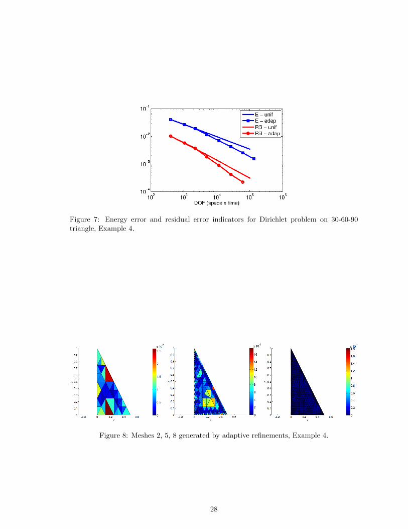
Figure 7: Energy error and residual error indicators for Dirichlet problem on 30-60-90triangle, Example 4.
Figure 8: Meshes 2, 5, 8 generated by adaptive refinements, Example 4.
28

rates are slightly reduced in Example 4, with angles of 30 degrees, possibly because of thenecessarily thin triangles in the triangulation.
10 Appendix: Mapping properties
We consider the mapping properties of Theorem 2.3, for Γ Lipschitz. The key step involvesestimates for a fundamental solution to the wave equation, from which the mapping prop-erties of the layer potentials can be deduced similarly as in Costabel’s work for the Laplaceequation [16].
Recall the following result by Becache and Ha Duong [8] for the Dirichlet trace:
Lemma 10.1. For s ∈ (12 ,
32), γ0 : Hs
ω,loc(Rd)→ Hs− 1
2ω (Γ) continuous and ‖γ0 u‖s− 1
2,ω,Γ .σ
‖u‖s,ω,Rd.
Becache and Ha Duong only state this result for s ≤ 1. The extension to s > 1 relies onthe approach of [16] for Lipschitz Γ. For Γ of class C1,α, continuity also holds for s = 3
2 , bythe extension in [48].
For x ∈ Rd \ Γ, the single layer operator for the Helmholtz equation is given by
Kω0 v(x) =
∫ΓGω(x, y)v(y) dsy = Gω γ∗0v(x) , (26)
where γ∗0 is the adjoint of the trace map γ0.As before, we always consider frequencies ω ∈ C with Imω > σ. Note that
1
iωGω : H−sω,comp(Rd)→ H−s+2
ω,loc (Rd) , (27)
because
‖ 1
iωGωv‖−s+2,ω,Rd = ‖F−1 1
iω(|ξ|2 − ω2)−1Fv‖−s+2,ω,Rd
= ‖(|ξ|2 + |ω|2)−s+2
21
iω(|ξ|2 − ω2)−1Fv‖L2(Rd)
≤ (Imω)−1 ‖(|ξ|2 + |ω|2)−s+2
2 (|ξ|2 + |ω|2)−1Fv‖L2(Rd)
= (Imω)−1 ‖v‖−s,ω,Rd .
Here
Re iω(|ξ|2 − ω2) = (Im ω)(|ξ|2 + |ω|2)
Hence
‖Gωf‖−s+2,ω,Rd .|ω|
Imω‖f‖−s,ω,Rd , (28)
so that with Imω ≥ σ
‖Kω0 v‖−s+2,ω,Rd .σ |ω|‖v‖−s+ 1
2,ω,Γ . (29)
29

From Lemma 10.1 we conclude that Vω := γ0Kω0 : H
− 12
+τω (Γ)→ H
12
+τω (Γ) continuously
for τ ∈ (−12 ,
12), and
‖Vωv‖ 12
+τ,ω,Γ .σ |ω|‖v‖− 12
+τ,ω,Γ . (30)
For x ∈ Rd \ Γ, the double layer potential for the Helmholtz equation is given by
Kω1 v(x) =
∫Γ∂ν(y)Gω(x, y)v(y) dsy. (31)
To describe the mapping properties of this operator, we rely on the following lemma:
Lemma 10.2. The Dirichlet problem
Pu := ∆u+ ω2u = 0 , (32a)
u|Γ = v, (32b)
for given v ∈ H12ω (Γ), admits a unique weak solution u = Tv, and
‖u‖1,ω,Ω . C(σ)|ω|‖v‖ 12,ω,Γ (33)
and
‖Tv‖H1P (Ω) :=
(‖u‖21,ω,Ω + ‖Pu‖20,ω,Ω
) 12 ≤ C ′(σ)|ω|‖v‖ 1
2,ω,Γ. (34)
Proof. The bilinear form
a(u, u) = −(∇u,∇u)L2(Ω) + ω2(u, u)L2(Ω) (35)
satisfies
Re
(−iω)
|ω|a(u, u)
= − Imω
|ω|‖u‖21,ω,Ω . (36)
Hence, the associated operator −iωA satisfies
‖A−1‖L(H−1ω (Ω),H1
ω(Ω)) ≤|ω|
Imω. (37)
We use the extension operator to extend v to v ∈ H1ω(Ω) with norm
‖v‖1,ω,Ω .σ ‖v‖ 12,ω,Γ. (38)
Then we seek a solution in H1ω,0(Ω) to Au = −Av ∈ H−1
ω (Ω). By (37), u exists and
‖u‖1,ω,Ω .σ|ω|
Imω‖v‖ 1
2,ω,Γ. (39)
To relate the double layer potential Kω1 to the solution operator T of (32), we use the
representation formula for x ∈ Rd \ Γ:
u(x) = Gωf(x) + 〈γ1Gω(x, ·), [γ0u]〉 − 〈[γ1u], Gω(x, ·)〉 . (40)
30

Here γ1 denotes the Neumann trace. This shows
Tv = −Kω1 v +Kω
0 γ1Tv, (41)
or
Kω1 = (−1 +Kω
0 γ1)T . (42)
With the operator norms from (29) and (34), we conclude
‖Kω1 v‖1,ω,Ω
.
(1 + ‖Kω
0 ‖L(H− 1
2ω (Γ),H1
ω(Ω))‖γ1‖
L(H1P (Ω),H
− 12
ω (Γ))
)‖T‖
L(H12ω (Γ),H1
P (Ω))‖v‖ 1
2,ω,Γ
.σ
(1 + |ω|‖γ1‖
L(H1P (Ω),H
− 12
ω (Γ))
)C ′(σ)|ω|‖v‖ 1
2,ω,Γ . (43)
It remains to determine ‖γ1‖L(H1
P (Ω),H− 1
2ω (Γ))
, which we now pursue.
The trace map γ0 admits a right-inverse γ−0 , which maps Hs−1/2ω (Γ)→ Hs
ω,loc(Rd) con-tinuously for all s ∈ (1/2, 1].
With
φ 7→ 〈γ1u, φ〉 := −a(u, γ−0 φ)−∫
ΩPu γ−0 φ , (44)
we have
supφ 6=0
|〈γ1u, φ〉|‖φ‖ 1
2,ω,Γ
= supφ 6=0
| − a(u, γ−0 φ)−∫
Ω Pu γ−0 φ|
‖φ‖ 12,ω,Γ
≤ supφ 6=0
| −∫
Ω ∂νu∂j(γ−0 φ) + ω2uγ−0 φ−
∫Ω Pu γ
−0 φ|
‖φ‖H
12 ,ω(Γ)
≤ supφ 6=0
1
‖φ‖ 12,ω,Γ
(‖∇u‖L2(Ω)‖∇γ−0 φ‖L2(Ω) + |ω|2‖u‖L2(Ω)‖γ−0 φ‖L2(Ω) + ‖Pu‖L2(Ω)‖γ−0 φ‖L2(Ω)
).σ sup
φ 6=0
1
‖γ−0 φ‖1,ω,Ω
[(‖∇u‖2L2(Ω) + |ω|2‖u‖2L2(Ω)
) 12(‖∇γ−0 φ‖
2L2(Ω) + |ω|2‖γ−0 φ‖
2L2(Ω)
) 12
+‖Pu‖L2(Ω)‖γ−0 φ‖L2(Ω)
].σ(‖∇u‖2L2(Ω) + |ω|2‖u‖2L2(Ω)
) 12
+ ‖Pu‖L2(Ω) (45)
Therefore we have for the conormal derivative γ1:
Lemma 10.3. Let u ∈ H1P (Ω). Then ϕ 7→ 〈γ1u, ϕ〉 is a continuous linear functional on
H12ω (Γ) and
‖γ1u‖− 12,ω,Γ .σ ‖u‖H1
P (Ω). (46)
31
We conclude for the double layer potential in the energy space:
‖Kω1 v‖1,ω,Ω .σ |ω| (1 + |ω|) ‖v‖ 1
2,ω,Γ. (47)
Variational arguments show that ‖Kω1 v‖1,ω,Ω .
|ω|Imω‖v‖ 1
2,ω,Γ. However, the above argument
generalizes (47) to arbitrary Sobolev exponents.
This generalization relies on the following theorem, which specifies the ω-dependenceof the endpoint estimates for the Dirichlet-Neumann and Neumann-Dirichlet operators,denoted by γ1T , respectively ND [34]:
Theorem 10.4. For all τ ∈ [−1/2, 1/2]:a) ‖γ1T‖L(H
τ+1/2ω (Γ),H
τ−1/2ω (Γ))
.σ |ω| ,
b) ‖ND‖L(Hτ−1/2ω (Γ),H
τ+1/2ω (Γ))
.σ |ω| .
Theorem 10.4 will be used to prove the following lemma:
Lemma 10.5. For τ ∈ [−12 ,
12 ], T : H
12
+τω (Γ)→ H1+τ
P (Ω) continuous and
‖Tv‖H1+τP (Ω) .σ |ω|‖v‖ 1
2+τ,ω,Γ. (48)
Lemma 10.6. For s ∈ (12 ,
32), γ1 : Hs
P (Ω)→ Hs− 3
2ω (Γ) continuous and
‖γ1u‖s− 32,ω,Γ .σ ‖u‖Hs
P (Ω) .
Proof. This follows from the Costabel’s trace theorem for ω = 1, ‖γ1u‖Hs− 3
2 (Γ). ‖u‖Hs(Ω),
using that s− 32 < 0:
‖γ1u‖s− 32,ω,Γ .σ ‖γ1u‖
Hs− 32 (Γ). ‖u‖Hs(Ω) .σ ‖u‖Hs
P (Ω) .
Proof of Lemma 10.5. Following [16], for a large enough ball B ⊇ Ω and Ω2 = B\Ω, weconsider
∆u+ ω2u = 0 in Ω2, (49a)
u|Γ = v, (49b)
u|∂B = 0 (49c)
with v ∈ H12
+τω (Γ). The solution operator is denoted by T2: u = T2v.
Let u =
Tv in Ω
T2v in Ω2
. Then we have
u = −Kω0 γ1u+
∫∂B∂νu(y) Gω(·, y) dsy, in Ω ∪ Ω2 (50)
By Theorem 10.4 we have for τ ∈ [−1/2, 1/2]
‖∂νu|∂B‖−1/2+τ,ω,∂B + ‖γ1Tv‖−1/2+τ,ω,Γ + ‖γ1T2v‖−1/2+τ,ω,Γ . |ω|‖v‖1/2+τ,ω,Γ
Therefore with (50) we have
‖u‖1+τ,ω,Ω . |ω|‖v‖1/2+τ,ω,Γ
yielding the assertion.
32
We now prove the estimates in Theorem 10.4. For these, we rely on frequency-explicitRellich identities, which we then translate into the time–domain.
Proof of Theorem 10.4. Applying the identity (5.1.1) and the Green’s formula (5.1.2) inNecas [34], yields with Av =
∑Nj=1 ∂
2j u+ ω2u and nkhk ≥ C > 0 that∫
∂Ω
(−hknk(∂iu)2 + 2(hi∂iu)(nk∂ku)
)=
∫Ω
(− (∂khk)(∂iu)2 + 2(∂khi)(∂iu)(∂ku)− 2hiω
2(∂iu)u). (51)
Here nk is the k-th component of the unit normal vector to Γ and h is a suitably chosenvector field.
Note that the left hand side is
2
∫∂Ω
((hi∂iu)(nk∂ku)− nkhk(∂iu)2
)+
∫∂Ωhknk(∂iu)2 .
Since the first integral only contains tangential derivatives,∑i
‖∂iu‖2L2(∂Ω) . ‖u|∂Ω‖2H1(∂Ω) +
∫Ω|Ou|2 + |ω|2
∣∣∣ ∫Ω
(hi∂iu)u∣∣∣ .
Hence ∑i
‖∂iu‖2L2(Γ) . ‖OΓu‖2L2(Γ) +
∫Ω|Ou|2 + |ω|2
∫Ω|∂u||u| (52)
Next we consider ∫Ω|Ou|2 − ω2|u|2 =
∫Γu|∂Ω(∂νu) . (53)
Taking the real part of (53) leads to∫Ω|Ou|2 +
(|Imω|2 − |Reω|2
)|u|2 = Re
∫Γu(∂νu) ,
while the imaginary part is given by
2(Imω)(Reω)
∫Ω|u|2 = Im
∫Γu(∂νu) .
We consider two cases: First, for |Reω| ≥ Imω2 ≥ σ
2 :∫Ω|u|2 . 1
|ω|Imω
∣∣∣ ∫Γu(∂νu)
∣∣∣ ,∫Ω|Ou|2
(53)
.(1 + |ω|)Imω
∣∣∣ ∫Γu(∂νu)
∣∣∣ ,∫Ω|Ou|2 + |ω|2|u|2 . (1 + |ω|)
Imω
∣∣∣ ∫Γu(∂νu)
∣∣∣ .
33
In the remaining case, |Reω| ≤ Imω2 (≥ σ
2 ), we have Imω '(|Imω|2 − |Reω|2
)1/2 '(|Imω|2 + |Reω|2
)1/2 ' |ω|, and with (53)∫Ω|Ou|2 + |ω|2|u|2 .
∣∣∣ ∫Γu(∂νu)
∣∣∣ ,∫Ω|ω|2|u||Ou| . |ω|2‖u‖L2(Ω)‖Ou‖L2(Ω) ,
‖Ou‖L2(Ω) .σ (1 + |ω|)1/2∣∣∣ ∫
Γu(∂νu)
∣∣∣1/2 ,‖u‖L2(Ω) .
1
|ω|1/2∣∣∣ ∫
Γu(∂νu)
∣∣∣1/2 .This implies ∫
Ω|Ou|2 + |ω|2|u||Ou| .σ |ω|2
∣∣∣ ∫Γu(∂νu)
∣∣∣ .Therefore (52) implies∑
i
‖∂iu‖2L2(Γ) .σ ‖OΓu‖2L2(Γ) + |ω|2‖u‖L2(Γ)‖∂νu‖L2(Γ) ,
∑i
‖∂iu‖L2(Γ) .σ ‖OΓu‖L2(Γ) + |ω|2‖u‖L2(Γ) ' |ω|‖u‖1,ω,Γ ,
i.e. Dirichlet data in H1ω(Γ) are mapped continuously to Neumann data in L2(Γ).
‖γ1T‖L(H1ω(Γ),L2(Γ)) .σ |ω| .
Standard arguments using the divergence theorem now show:∫Ωdiv(|u|2h) =
∫Ω|u|2divh+ 2Re
∫Ωu(h · Ou)
.∫
Ω|u|2 +
∫Ω|u||Ou|
.σ1
|ω|
∣∣∣ ∫Γu∂νu
∣∣∣+ ‖u‖L2(Ω)‖Ou‖L2(Ω)
.σ
(1
|ω|+ 1
) ∣∣∣ ∫Γu∂νu
∣∣∣.
(1
|ω|+ 1
)(ε‖u‖2L2(Γ) +
1
ε‖∂νu‖2L2(Γ)
)1/2
,
where 0 < ε . |ω||ω|+1 . Therefore,
‖u‖L2(Γ) ≤(
1
|ω|+ 1
)2
‖∂νu‖L2(Γ).
Using (51) as in the proof of Lemma 5.2.2 in [34], we conclude:∫Γ
(−hknk(∂iu)2 + 2(hi∂iu)(nk∂ku)
)≤∫
Ω
(|Ou|2 + |ω|2|Ou||u|
).
34
Note that the left hand side is larger than∫
Γ
∑i(∂iu)2 − C
∑i|∂iu||∂νu|, so that∫
Γ
∑i
|∂iu|2 .∫
Γ(∂νu)2 +
∫Ω
(|Ou|2+|ω|2|Ou||u|
).
As above, ∫Ω
(|Ou|2 + |ω|2|Ou||u|
).σ |ω|2
∣∣∣ ∫Γu∂νu
∣∣∣ ,so that ∑
i
∫Γ|∂iu|2 .
∫Γ(∂νu)2 + |ω|4‖u‖2L2(Γ)
. |ω|2‖u‖21,ω,Γ .
Altogether, we conclude the endpoint estimate ‖γ1T‖L(H1ω(Γ),L2(Γ)) .σ |ω|.
Further, as in [34], Theorem 5.1.3, γ1T extends by duality to a bounded linear operatorfrom L2(Γ) to H−1
ω (Γ) and
‖γ1T‖L(L2(Γ),H−1ω (Γ)) .σ |ω| .
By interpolation, we conclude for τ ∈ [−1/2, 1/2]
‖γ1T‖L(Hτ+1/2ω (Γ),H
τ−1/2ω (Γ)
.σ |ω| .
Similar arguments apply to the Neumann-Dirichlet operator ND. They lead to
‖ND‖L(H−1ω (Γ),L2(Γ)) .σ |ω| ,
and then by duality and interpolation for τ ∈ [−12 ,
12 ]
‖ND‖L(Hτ−1/2ω (Γ),H
τ+1/2ω (Γ))
.σ |ω| .
We finally prove Theorem 2.3.
Proof of Theorem 2.3. From above we recall for τ ∈ [−12 ,
12 ]
‖Kω0 v‖1+τ,ω,Ω .σ |ω|‖v‖−1/2+τ,ω,Γ , (54)
and for τ ∈ (−12 ,
12)
‖Vωv‖1/2+τ,ω,Γ = ‖γ0Kω0 v‖1/2+τ,ω,Γ .σ |ω|‖v‖−1/2+τ,ω,Γ , (55)
‖K′ωv‖−1/2+τ,ω,Γ = ‖γ1Kω0 v‖−1/2+τ,ω,Γ .σ |ω|‖v‖−1/2+τ,ω,Γ . (56)
From the proof of Lemma 10.5, (42) and the trace theorem we obtain for τ ∈ [−12 ,
12 ]
‖Kω1 v‖1+τ,ω,Ω .σ |ω|2‖v‖1/2+τ,ω,Γ , (57)
generalizing (47). We conclude for τ ∈ (−12 ,
12)
‖Kωv‖1/2+τ,ω,Γ = ‖γ0Kω1 v‖1/2+τ,ω,Γ .σ |ω|2‖v‖1/2+τ,ω,Γ , (58)
‖Wωv‖−1/2+τ,ω,Γ = ‖γ1Kω1 v‖−1/2+τ,ω,Γ .σ |ω|2‖v‖1/2+τ,ω,Γ . (59)
Using the Fourier transform to translate back into the time domain, we conclude the proofof Theorem 2.3 for Γ Lipschitz.
For Γ of class C1,α, the Dirichlet and Neumann traces γ0 and γ1 are also continuous inthe endpoints of the interval τ ∈ [−1
2 ,12 ], and the estimates (55), (56), (58) and (59) extend
to the endpoints τ = ±12 .
35
References
[1] A. Aimi, M. Diligenti, A. Frangi, C. Guardasoni, Neumann exterior wave propagationproblems: computational aspects of 3D energetic Galerkin BEM, Comput. Mech. 51(2013), 475–493.
[2] A. Aimi, M. Diligenti, A. Frangi, C. Guardasoni, A stable 3D energetic Galerkin BEMapproach for wave propagation interior problems, Eng. Anal. Bound. Elem. 36 (2012),1756–1765.
[3] A. Aimi, M. Diligenti, C. Guardasoni, On the energetic Galerkin boundary elementmethod applied to interior wave propagation problems, J. Comput. Appl. Math. 235(2011), 1746–1754.
[4] A. Aimi, M. Diligenti, C. Guardasoni, I. Mazzieri, S. Panizzi, An energy approach tospace-time Galerkin BEM for wave propagation problems, Internat. J. Numer. MethodsEngrg. 80 (2009), 1196–1240.
[5] A. Bamberger, T. Ha Duong, Formulation variationnelle espace-temps pour le calculpar potentiel retard de la diffraction d’une onde acoustique, Math. Meth. Appl. Sci. 8(1986), 405–435.
[6] A. Bamberger, T. Ha Duong, Formulation variationnelle pour le calcul de la diffractiond’une onde acoustique par une surface rigide, Math. Meth. Appl. Sci. 8 (1986), 598608.
[7] L. Banz, H. Gimperlein, Z. Nezhi, E. P. Stephan, Time domain BEM for sound radi-ation of tires, Computational Mechanics 58 (2016), 45–57.
[8] E. Becache, T. Ha-Duong, A space-time variational formulation for the boundary in-tegral equation in a 2D elastic crack problem, RAIRO Model. Math. Anal. Numer. 28(1994), 141–176.
[9] E. Becache, A variational boundary integral equation method for an elastodynamicantiplane crack, Internat. J. Numer. Methods Engrg. 36 (1993), 969-984.
[10] C. Carstensen, Merging the Bramble-Pasciak-Steinbach and the Crouzeix-Thomee cri-terion for H1-stability of the L2-projection onto finite element spaces, Math. Comp. 71(2002), 157-163.
[11] C. Carstensen, Efficiency of a posteriori BEM-error estimates for first-kind integralequations on quasi-uniform meshes, Math. Comp. 65 (1996), 69–84.
[12] C. Carstensen, D. Praetorius, Averaging techniques for the effective numerical solutionof Symm’s integral equation of the first kind, SIAM J. Sci. Comp. 27 (2006), 1226–1260.
[13] C. Carstensen, E. P. Stephan, A posteriori error estimates for boundary element meth-ods, Math. Comp. 64 (1995), 483–500.
[14] C. Carstensen, M. Maischak, E. P. Stephan, A posteriori error estimate and h-adaptivealgorithm on surfaces for Symm’s integral equation, Numer. Math. 90 (2001), 197–213.
[15] C. Carstensen, M. Maischak, D. Praetorius, E. P. Stephan, Residual-based a posteriorierror estimate for hypersingular equation on surfaces, Numer. Math. 97 (2004), 397–426.
[16] M. Costabel, Boundary integral operators on Lipschitz domains: elementary results,SIAM J. Math. Anal. 19 (1988), 613–626.
36
[17] M. Costabel, F.-J. Sayas, Time-dependent problems with the boundary integral equationmethod. in: Encyclopedia of Computational Mechanics, Second Edition, E. Stein, R. deBorst and J. R. Hughes (Eds.), 2017, pp. 1–24.
[18] B. Faermann, Local a-posteriori error indicators for the Galerkin discretization ofboundary integral equations, Numer. Math. 79 (1998), 43–76.
[19] B. Faermann, Localization of the Aronszajn-Slobodeckij norm and application to adap-tive boundary element methods. II. The three-dimensional case, Numer. Math. 92(2002), 467–499.
[20] H. Gimperlein, M. Maischak, E. P. Stephan, Adaptive time domain boundary elementmethods and engineering applications, Journal of Integral Equations and Applications29 (2017), 75–105.
[21] H. Gimperlein, F. Meyer, C. Ozdemir, E. P. Stephan, Time domain boundary ele-ments for dynamic contact problems, Computer Methods in Applied Mechanics andEngineering 333 (2018), 147–175.
[22] H. Gimperlein, F. Meyer, C. Ozdemir, D. Stark, E. P. Stephan, Boundary elements withmesh refinements for the wave equation, Numerische Mathematik 139 (2018), 867–912.
[23] H. Gimperlein, Z. Nezhi, E. P. Stephan, A priori error estimates for a time-dependentboundary element method for the acoustic wave equation in a half-space, MathematicalMethods in the Applied Sciences 40 (2017), 448–462.
[24] H. Gimperlein, C. Ozdemir, E. P. Stephan, Time domain boundary element methodsfor the Neumann problem: Error estimates and acoustic problems, Journal of Compu-tational Mathematics 36 (2018), 70–89.
[25] H. Gimperlein, C. Ozdemir, D. Stark, E. P. Stephan, hp-version time domain bound-ary elements for the wave equation on quasi-uniform meshes, Computer Methods inApplied Mechanics and Engineering 356 (2019), 145–174.
[26] M. Glaefke, Adaptive Methods for Time Domain Boundary Integral Equations, PhDthesis, Brunel University, 2012.
[27] J. Gwinner, E. P. Stephan, Advanced Boundary Element Methods – Treatment ofBoundary Value, Transmission and Contact Problems, Springer Series in Computa-tional Mathematics 52, Springer, 2018.
[28] T. Ha Duong, Equations integrales pour la resolution numerique des problemes dediffraction d’ondes acoustiques dans R3, Ph.D. thesis, Paris VI, 1987.
[29] T. Ha-Duong, On the transient acoustic scattering by a flat object, Japan J. Appl.Math. 7 (1990), 489-513.
[30] T. Ha Duong, On retarded potential boundary integral equations and their discretiza-tions, in: Topics in computational wave propagation, pp. 301-336, Lect. Notes Com-put. Sci. Eng., 31, Springer, Berlin, 2003.
[31] P. Joly, J. Rodriguez, Mathematical aspects of variational boundary integral equationsfor time dependent wave propagation, J. Integral Equations Appl. 29 (2017), 137-187.
37
[32] A. Y. Kokotov, P. Neittaanmaki, B. A. Plamenevskiı, The Neumann problem for thewave equation in a cone, J. Math. Sci. 102 (2000), 4400–4428.
[33] A. Y. Kokotov, P. Neittaanmaki, B. A. Plamenevskiı, Diffraction on a cone: Theasymptotics of solutions near the vertex, J. Math. Sci. 109 (2002), 1894–1910.
[34] J. Necas, Les methodes directes en theorie des equations elliptiques Masson, Paris, 1967.
[35] F. Muller, C. Schwab, Finite elements with mesh refinement for wave equations inpolygons, J. Comput. Appl. Math. 283 (2015), 163–181.
[36] B. A. Plamenevskiı, On the Dirichlet problem for the wave equation in a cylinder withedges, Algebra i Analiz 10 (1998), 197–228.
[37] T. von Petersdorff, Randwertprobleme der Elastizitatstheorie fur Polyeder-Singularitaten und Approximation mit Randelementmethoden, Ph.D. thesis, TechnischeUniversitat Darmstadt (1989).
[38] T. von Petersdorff, E. P. Stephan, Regularity of mixed boundary value problems in R3
and boundary element methods on graded meshes, Math. Methods Appl. Sci. 12 (1990),229–249.
[39] T. von Petersdorff, E. P. Stephan, Decompositions in edge and corner singularities forthe solution of the Dirichlet problem of the Laplacian in a polyhedron, Math. Nachr. 149(1990), 71–103.
[40] S. Sauter, A. Veit, Adaptive Time Discretization for Retarded Potentials, Nu-mer. Math. 132 (2016), 569–595.
[41] S. Sauter, M. Schanz, Convolution quadrature for the wave equation with impedanceboundary conditions, J. Comp. Phys. 334 (2017), 442–459.
[42] F.-J. Sayas, Retarded Potentials and Time Domain Boundary Integral Equations: ARoad Map, Springer Series in Computational Mathematics 50, Springer, 2016.
[43] O. Steinbach, Stability estimates for hybrid coupled domain decomposition methods,Lecture Notes in Mathematics 1809, Springer, 2003.
[44] O. Steinbach, C. Urzua-Torres, A New Approach to Time Domain Boundary IntegralEquations for the Wave Equation, Oberwolfach Reports 17 (2020), in proceedings ofWorkshop 2006a: Boundary Element Methods.
[45] A. Veit, Numerical methods for time-domain boundary integral equations, Ph.D. thesis,Universitat Zurich (2012).
[46] A. Veit, M. Merta, J. Zapletal, D. Lukas, Efficient solution of time-domain boundaryintegral equations arising in sound-hard scattering, Internat. J. Numer. Meth. Eng. 107(2016), 430–449.
[47] G. Verchota, Layer potentials and regularity for the Dirichlet problem for Laplace’sequation in Lipschitz domains, Journal of Functional Analysis 59 (1984), 572–611.
[48] W. Wendland, Martin Costabel’s version of the trace theorem revisited, MathematicalMethods in the Applied Sciences 40 (2017), 329–334.
38