borehole heat flow along the eastern flank of the juan de...

Borehole heat flow along the eastern flank of the Juan de Fuca Ridge,including effects of anisotropy and temperature

dependence of sediment thermal conductivity- Appendix -

Dan F.C. Pribnow Joint Geoscientific Research Institute, GGA

Stilleweg 2D-30655 Hannover, Germany

Earl E. DavisPacific Geoscience Centre, PGC

Geological Survey of CanadaP.O. Box 6000

Sidney, B.C. V8L 4B2Canada

Andrew T. FisherEarth Sciences Department and Institute of Tectonics

University of Santa Cruz, CaliforniaSanta Cruz, CA 95064

USA

Appendix

A1. IntroductionThis Appendix contains detailed descriptions of experimental and analytical methods used

in this study. The divided bar method to determine thermal conductivity is described,emphasising aspects of anisotropy in comparison to the needle probe approach and effects oftemperature. The influence of porosity and sea water properties on anisotropy and temperatureeffects is discussed. Various methods for the calculation of thermal resistance are presentedand evaluated. Finally, the consequences for the heat flow calculation are analyzed.

A2. Divided-Bar Thermal Conductivity MeasurementsA2.1 The Divided-Bar Method

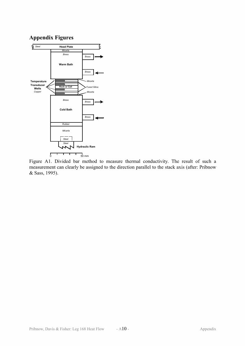
There are two major differences between divided-bar and ship-board line-source thermalconductivity methods: (1) the line-source method is transient while the divided-bar is steady-state; (2) divided-bar measurements provide one-dimensional data (Fig. A1), whereas the line-source method produces a scalar value from a plane (Fig. A2). The ability to measure thermalconductivity in a single direction makes the divided-bar method suitable for the determinationof anisotropy (e.g., Pribnow and Sass, 1995).

The divided-bar is a comparative method in which the temperature drop across a disk ofrock or a cylindrical cell containing water-saturated material is compared with that across adisk of reference material of known thermal conductivity (Fig. A1; see also Sass et al., 1992;Pribnow and Sass, 1995). It is in theory and by design a one-dimensional method to determinethermal conductivity parallel to the divided-bar axis. Samples are prepared with theircylindrical axis parallel to the desired direction of conductivity to be determined. The

Pribnow, Davis & Fisher: Leg 168 Heat Flow - A1 - Appendix

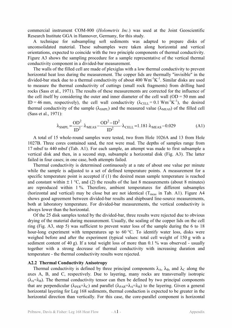
commercial instrument COM-800 (Holometrix Inc.) was used at the Joint GeoscientificResearch Institute GGA in Hannover, Germany, for this study.

A technique for subsampling soft sediments was adapted to prepare disks ofunconsolidated material. These subsamples were taken along horizontal and verticalorientations, expected to coincide with the two principle components of thermal conductivity.Figure A3 shows the sampling procedure for a sample representative of the vertical thermalconductivity component in a divided-bar measurement.

The walls of the filled cell are made of plexiglas with a low thermal conductivity to preventhorizontal heat loss during the measurement. The copper lids are thermally "invisible" in thedivided-bar stack due to a thermal conductivity of about 400 Wm-1K-1. Similar disks are usedto measure the thermal conductivity of cuttings (small rock fragments) from drilling hardrocks (Sass et al., 1971). The results of these measurements are corrected for the influence ofthe cell itself by considering the outer and inner diameter of the cell wall (OD = 50 mm andID = 46 mm, respectively), the cell wall conductivity (λCELL = 0.1 Wm-1K-1), the desiredthermal conductivity of the sample (λSMPL) and the measured value (λMEAS) of the filled cell(Sass et al., 1971):

029.0181.1ID

IDODIDOD

MEASCELL2

22

MEAS2

2

SMPL −λ⋅=λ⋅−−λ⋅=λ (A1)

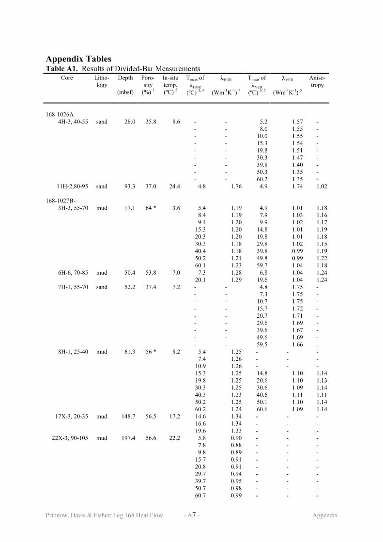
A total of 15 whole-round samples were tested, two from Hole 1026A and 13 from Hole1027B. Three cores contained sand, the rest were mud. The depths of samples range from17 mbsf to 440 mbsf (Tab. A1). For each sample, an attempt was made to first subsample avertical disk and then, in a second step, subsample a horizontal disk (Fig. A3). The latterfailed in four cases; in one case, both attempts failed.

Thermal conductivity is determined continuously at a rate of about one value per minutewhile the sample is adjusted to a set of defined temperature points. A measurement for aspecific temperature point is accepted if (1) the desired mean sample temperature is reachedand constant within ± 1 °C, and (2) the results of the last 8 measurements (about 8 minutes)are reproduced within 1 %. Therefore, ambient temperatures for different subsamples(horizontal and vertical) may be close but are not identical (Tmeas in Tab. A1). Figure A4shows good agreement between divided-bar results and shipboard line-source measurements,both at laboratory temperature. For divided-bar measurements, the vertical conductivity isalways lower than the horizontal.

Of the 25 disk samples tested by the divided-bar, three results were rejected due to obviousdrying of the material during measurement. Usually, the sealing of the copper lids on the cellring (Fig. A3, step 5) was sufficient to prevent water loss of the sample during the 6 to 18hour-long experiment with temperatures up to 60 °C. To identify water loss, disks wereweighed before and after the experiment (typical values: total cell weight of 150 g with asediment content of 40 g). If a total weight loss of more than 0.1 % was observed - usuallytogether with a strong decrease of thermal conductivity with increasing duration andtemperature - the thermal conductivity results were rejected.

A2.2 Thermal Conductivity AnisotropyThermal conductivity is defined by three principal components λA, λB, and λC along the

axes A, B, and C, respectively. Due to layering, many rocks are transversally isotropic(λA=λB). The thermal conductivity tensor can then be defined by two principal componentsthat are perpendicular (λPER=λC) and parallel (λPAR=λA=λB) to the layering. Given a generalhorizontal layering for Leg 168 sediments, thermal conduction is expected to be greater in thehorizontal direction than vertically. For this case, the core-parallel component is horizontal


(λHOR=λPAR) and the perpendicular component is vertical (λVER=λPER). In this study, we definethe thermal conductivity anisotropy K as (e.g., Popov et al., 1999):

PER

PAR

VER

HORKλλ

=λλ

= (A2)

For heat flow calculations, the vertical component of thermal conductivity, which isparallel to the direction of the measured temperature gradient, was calculated using line-source values and the assumed anisotropy. The line-source provides a two-dimensional valueof thermal conductivity (λLS) for a plane perpendicular to the needle axis (Fig. A2). The resultobtained from a measurement of an anisotropic sample is related to the orientations of theprincipal axes of the thermal conductivity tensor (λA, λB, λC):

)(cos)(cos)(cos 2CB

2CA

2BALS α⋅λ⋅λ+β⋅λ⋅λ+γ⋅λ⋅λ=λ (A3)

where α, β, and γ are angles between the line-source axis and principal axes of thermalconductivity A, B, and C, respectively (Popov et al., 1999). Considering the horizontalposition of the line-source for routine measurements performed during Leg 168 (Fig. A2) andthe horizontal anisotropy of Leg 168 sediments, α = 0° and β = γ = 90°, equation (A3) can besimplified to

VERHORLS λ⋅λ=λ (A4)

Therefore, in case the needle probe is positioned parallel to the bedding, the measured thermalconductivity is the geometric mean of the parallel and perpendicular components. The desiredvertical component of thermal conductivity is calculated as:

)z(K)z(

)z( LSVER

λ=λ (A5)

A2.3 Temperature Dependence of Thermal ConductivityFor 12 of the 22 samples with acceptable results from divided-bar measurements

(horizontal and vertical), thermal conductivity was measured within a temperature rangebetween 5 °C and 60 °C, and for 10 of these, at 20 °C and at the corresponding in-situtemperature (Tab. A1 and Fig. 5). The effect of temperature is related to the thermalconductivity at laboratory (room) temperature, λrt = λ(20 °C): if λrt is low, conductivityincreases with temperature; if λrt is intermediate, conductivity does not change withtemperature; if λrt is high, conductivity decreases with temperature. Figure A5 shows a lineartemperature dependence of thermal conductivity (∆λ/∆T) as a function of λrt. The linearregression of this dataset provides a means to calculate a value of thermal conductivity for anytemperature based only on λrt:

)20T()107.4104.5(

)20T(T/)T(

rt33

rt

rt

−⋅λ⋅⋅−⋅+λ=

−⋅∆λ∆+λ=λ−− (A6)

Thus, the correction can be applied directly to shipboard laboratory values by substituting λLS

for λrt in equation (A6). The depth of a sample is translated into an in-situ temperature withthe average temperature gradient of the corresponding hole (Fig. 2).

A2.4 The Influence of PorosityIn this brief discussion, anisotropy and temperature corrections are generalized for cases

where only porosity and line-source thermal conductivity values are available. The amount of


porewater in the sample has influence on both anisotropy and temperature effects. Water isisotropic and decreases the bulk anisotropy with increasing porosity for a sample withanisotropic matrix. The temperature dependence of water is different from that of the matrix.To separate these effects, the geometric mixing model is used:

φ−φ λ⋅λ=λ 1MATFLDBLK (A7)

where φ is porosity, and the subscripts BLK, FLD and MAT stand for bulk, fluid, and matrix,respectively. It is noteworthy that the geometric mean is a simple and robust mixing modelthat is widely used, but not physically based (Woodside and Messmer, 1961; Sass et al., 1971;Pribnow and Umsonst, 1993; Pribnow and Sass, 1995). Sample porosities for this study weremeasured during Leg 168 (Davis et al., 1997a) and are listed in Table A1.

A2.4.1 Anisotropy. Based on the geometric mean model (eq. A7), the matrix anisotropycan be estimated by:

φ−φ−φ

φ−φ

=λ⋅λ

λ⋅λ= 1

MAT1v,MATFLD

1h,MATFLD

BLK KK , (A8)

where K is anisotropy (eq. A2), and subscripts v and h represent vertical and horizontalcomponents, respectively. For this study, the average of the matrix anisotropy calculated withequation (A8) is KMAT = 1.4 ± 0.2. Davis and Seemann (1994) suggest a mean matrixconductivity of 3.3 Wm-1K-1 for the horizontal and 2.6 Wm-1K-1 for the vertical component,indicating similar matrix anisotropy of KMAT = 1.3. With equations (A6) to (A8) and anassumed matrix conductivity, the bulk vertical conductivity can be calculated from shipboardline-source measurements (λLS) and sample porosity (φ) with:

( ) φ−

λ=λ

1 MAT

LSVER

K

)z()z( (A9)

A2.4.2 Temperature Dependence. The temperature dependence between 0 °C and 60 °Cof sea water, λFLD(T), and matrix, λMAT(T), can be represented by (see Tab. A2):

T1044.156.0)T( 3FLD ⋅⋅+=λ − (A10 a)

T1011.593.2)T( 3MAT ⋅⋅−=λ − (A10 b)

with T in °C. Based on the geometric mixing model, the general temperature dependence ofthe bulk conductivity can be expressed by:

)T()T()T( 1MATFLDBLK

φ−φ λ⋅λ=λ (A11)

This approach is supported by the good agreement between measured and calculated (eq. A11)temperature dependence (Fig. 5).

An analysis similar to that used for bulk conductivity yields a linear temperaturedependence of matrix thermal conductivity as a function of conductivity at laboratorytemperature (Fig. A6). Whereas the bulk conductivity shows both positive and negativetemperature coefficients depending on sediment porosity, matrix conductivity generallydecreases with increasing temperature, particularly at high λrt values. Adapting equation (A11)for λrt and considering that λFLD(20 °C) = 0.6 Wm-1K-1, an equation describing thetemperature dependence of matrix thermal conductivity for Leg 168 sediments based onsample porosity and laboratory temperature values is similar to equation (A6):


)20T( )6.0(

104.5100.8)6.0(

)T(1

1

rt3311

rtMAT −⋅

λ⋅⋅−⋅+

λ=λ

φ−

φ−−φ−

φ (A12)

When combined with equation (A10a and A11), this allows estimation of in-situ bulk thermalconductivity from λrt, porosity, and temperature data alone.

A3 Thermal ResistanceBased on the experimental thermal conductivity anisotropy and temperature dependence,

we calculated vertical thermal resistance values (Ω) along the Leg 168 transect. Depths andthicknesses of sediment layers are generally well known from shipboard observations,although core recovery was poor in sandy intervals (Davis et al., 1997a). One standardapproach is to assume that each conductivity value λk, at depth zλ,k, is representative of a layerbetween zλ,k and zλ,k-1, the next shallowest measurement:

λ−

=Ω −λλ

k

1k,k, zz(A13)

This approach is inappropriate in this case because sandy intervals are often skipped betweenwidely spaced measurements. Instead, we estimate the thermal resistance based on averagethermal conductivity values for sand and mud, λS and λM, and then we use core descriptions toassign sand and mud layers.

The thermal resistance is calculated for the interval between two temperaturemeasurements Tj-1 and Tj, at depths zΤ,j-1 and zΤ,j, with the harmonic mean and weighted by thetotal thickness dS,j and dM,j of sand and mud layers within this depth interval:

λ+

λ⋅

−+Ω=Ω

−−

M

j,M

S

j,S

1j,Tj,T1j,Tj,T

ddzz

1)z()z( (A14)

This shipboard approach (Davis et al., 1997a) neglects any depth dependence on porosityand thermal conductivity. We now account for the porosity decrease with depth by: (1)calculating the thermal resistance of mud (ΩM,j) with equation (A13) for the interval betweentwo temperature measurements Tj-1 and Tj (zΤ,j - zΤ,j-1), based on individual measurements inmud (λM,k); (2) calculating the thermal resistance of sand layers (ΩS,j) in the same depthinterval with equation (A14), based on an average value for sand (λS,j) because themeasurements do not indicate a systematic change with depth; and (3) combining the tworesistance values, weighted with the total thickness dS,j and dM,j of sand and mud layers (asdetermined by shipboard core descriptions), in relation to the depth interval zΤ,j - zΤ,j-1:

( )

λ−

⋅+λ

⋅⋅−

+Ω=

Ω⋅+Ω⋅⋅−

+Ω=Ω

−

−−

−−

k,M

1k,Mk,Mj,M

j,S

j,Sj,S

1j,Tj,T1j,T

j,Mj,Mj,Sj,S1j,Tj,T

1j,Tj,T

zzd

dd

zz1)z(

ddzz

1)z()z(

(A15)

In this way, both systematic changes in mud conductivity and the occurance of sand layers areincluded in the analysis. Figure A7 shows an example for the calculation of thermal resistancewith equation (A15) for a layer between two temperature measurements in Hole 1023A.

A4 Heat Flow Calculations


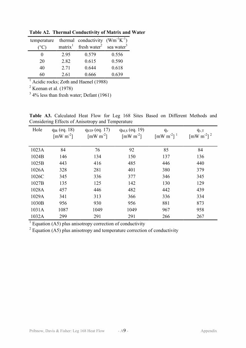
To evaluate the significance of this method for thermal resistance calculation plus theconsideration of anisotropy and temperature effects on conductivity, the recalculation of heatflow is performed in several steps. qIR is shipboard heat flow (Davis et al., 1997a), using oneaverage thermal conductivity for mud and one for sand (eq. A14), ignoring variations inconductivity with depth but considering each layer. qSTP is heat flow calculated from athermal resistance that is based on all conductivity values (eq. A13), considering variationswith depth but neglecting layers not represented by measurements. qM,S is heat flow based ona combination of using the qIR method for sand layers and the qSTP method for mud layers (eq.A15), thus considering variations with depth for mud and each sand layer. qv is the qM,Smethod based on vertical conductivity corrected for mud anisotropy (A5); qv,T is the qM,Smethod based on vertical conductivity corrected for anisotropy (A5) and temperature (eq. A6);for the mean sand conductivity of a layer (λS,j), the average conductivity at laboratorytemperature for sand (1.53 Wm-1K-1) is corrected for the in-situ temperature (eq. A6), which isrelevant in the considered depth interval.

Table A3 lists all previous and revised heat flow values. The relative differences arediscussed in relation to the used methods. qSTP vs qIR: Consideration of the observed thermalconductivity decrease close to seafloor (Fig. 3) by using the qSTP method results in heat flowvalues that are 2 % to 14 % lower than those based on constant mud conductivity (qIR). Thelargest change occurs for Hole 1026A (-14 %), where 30 % of the drilled section comprisessand (Davis et al., 1997a). These layers with higher conductivity are considered fully in the qIRmethod but neglected in the qSTP method, unless the number of conductivity measurementsfrom sand layers is representative. qM,S vs qSTP: Consideration of all sand layers (qM,S) has noeffect on measurements in a pure mud environment (1031A, 1032A) but increases heat flowby up to 43 % (Hole 1026A), where sand layers occur. qv vs qM,S: Due to anisotropy, thevertical conductivity reduces heat flow values by 5 % to 9 %. qv,T vs qv: Correcting verticalconductivity for temperature causes a negligible (less than 1 %) decrease of heat flow. qv,T vsqIR: After improving resistivity calculations and correcting for anisotropy and temperature(qv,T), heat flow is reduced by up to 12 % for all sites except 1026A, where qv,T is 16 %higher. The general reduction of heat flow results from lower vertical conductivity in thisstudy, although at Hole 1026A, this effect is overwhelmed by inclusion of thick sand layers.The impact of the temperature correction is generally small because thermal conductivityvalues at laboratory temperature are close to 1.2 Wm-1K-1 (Fig. A3).

Consequences of these additional aspects for Leg 168 borehole heat flow are: (1) a 2 % to14 % decrease resulting from consideration of low conductivities of high-porous sedimentsclose to seafloor (upper 5 mbsf); (2) an increase up to 20 % by considering all known sandlayers with higher conductivity; (3) a 5 % to 9 % decrease resulting from the use of verticalconductivity; and (4) a decrease less than 1% based on temperature corrections.


Appendix ReferencesDavis, E.E., and D.A. Seemann, Anisotropic thermal conductivity of pleistocene turbidite

sediments of the northern Juan de Fuca Ridge, Proceedings of the Ocean DrillingProgram, Scientific Results, Vol. 139, 559 - 564, 1994.

Davis, E.E., A.T. Fisher, J.V. Firth et al., Proceedings of the Ocean Drilling Program, InitialResults, Vol. 168, pp. 470, 1997a.

Davis, E.E., D.S. Chapman, H. Villinger, S. Robinson, J. Grigel, A Rosenberger, and D.F.C.Pribnow, Seafloor heat flow on the eastern flank of the Juan de Fuca Ridge: data from”FlankFlux” studies through 1995, Proceedings of the Ocean Drilling Program, InitialResults, Vol. 168, 23 - 33, 1997b.

Davis, E.E., D.S. Chapman, K. Wang, H. Villinger, A.T. Fisher, S.W. Robinson, J. Grigel,D.F.C. Pribnow, J. Stein, and K. Becker, Regional heat-flow variations across thesedimented Juan de Fuca Ridge and lateral hydrothermal heat transport, J. Geophys.Res., 104, 17675-17688, 1999.

Defant, A., Physical Oceanography, Vol. 1, Pergamon, New York, NY, 1961.Keenan, J.H., F.G. Keyes, P.G. Hill, and J.G Moore, Steam Tables: Thermodynamic

Properties of Water, Including Vapor, Liquid, and Solid Phases, Wiley, New York, NY,1978.

Popov Y.A, D.F.C. Pribnow, J.H. Sass, C.F. Williams, and H. Burkhardt, Characterization ofrock thermal conductivity by high-resolution optical scanning, Geothermics, in press,1999.

Pribnow, D.F.C., and J.H. Sass, Determination of thermal conductivity for deep boreholes, J.Geophys. Res., 100, 9981 - 9994, 1995.

Pribnow, D.F.C., and T. Umsonst, Estimation of thermal conductivity from the mineralcomposition: influence of fabric and anisotropy, Geophys. Res. Let., 20, 2199-2202,1993.

Sass, J.H., A.H. Lachenbruch, and R. Munroe, Thermal conductivity of rocks frommeasurements on fragments and its application to heat flow determinations, J. Geophys.Res., 76, 3391 - 3401, 1971.

Sass, J.H., A.H. Lachenbruch, T. Moses, and P. Morgan, Heat flow from a scientific researchwell at Cajon Pass, California, J. Geophys. Res., 97, 5017 - 5030, 1992.

Woodside, W., and J. Messmer, Thermal conductivity of porous media, J. Appl. Phys., 32,1688-1706, 1961.

Zoth, G., and R. Hänel, Appendix, in: R. Hänel, L. Rybach and I. Stegena (eds), Handbook ofTerrestrial Heat-Flow Density Determination, Kluwer Academic Publishers, Dordrecht,pp. 449-466, 1988.


Appendix TablesTable A1. Results of Divided-Bar Measurements

Core Litho-logy

Depth

(mbsf)

Poro-sity

(%) 1

In-situtemp.(ºC) 2

Tmeas ofλHOR

(ºC) 3, 4

λHOR

(Wm-1K-1) 4

Tmeas ofλVER

(ºC) 3, 5

λVER

(Wm-1K-1) 5

Aniso-tropy

168-1026A-4H-3, 40-55 sand 28.0 35.8 8.6 - - 5.2 1.57 -

- - 8.0 1.55 -- - 10.0 1.55 -- - 15.3 1.54 -- - 19.8 1.51 -- - 30.3 1.47 -- - 39.8 1.40 -- - 50.3 1.35 -- - 60.2 1.35 -

11H-2,80-95 sand 93.3 37.0 24.4 4.8 1.76 4.9 1.74 1.02

168-1027B-3H-3, 55-70 mud 17.1 64 * 3.6 5.4 1.19 4.9 1.01 1.18

8.4 1.19 7.9 1.03 1.169.4 1.20 9.9 1.02 1.17

15.3 1.20 14.8 1.01 1.1920.3 1.20 19.8 1.01 1.1830.3 1.18 29.8 1.02 1.1540.4 1.18 39.8 0.99 1.1950.2 1.21 49.8 0.99 1.2260.1 1.23 59.7 1.04 1.18

6H-6, 70-85 mud 50.4 53.8 7.0 7.3 1.28 6.8 1.04 1.2420.1 1.29 19.6 1.04 1.24

7H-1, 55-70 sand 52.2 37.4 7.2 - - 4.8 1.75 -- - 7.3 1.75 -- - 10.7 1.75 -- - 15.7 1.72 -- - 20.7 1.71 -- - 29.6 1.69 -- - 39.6 1.67 -- - 49.6 1.69 -- - 59.5 1.66 -

8H-1, 25-40 mud 61.3 56 * 8.2 5.4 1.25 - - -7.4 1.26 - - -

10.9 1.26 - - -15.3 1.25 14.8 1.10 1.1419.8 1.25 20.6 1.10 1.1330.3 1.25 30.6 1.09 1.1440.3 1.23 40.6 1.11 1.1150.2 1.25 50.1 1.10 1.1460.2 1.24 60.6 1.09 1.14

17X-3, 20-35 mud 148.7 56.5 17.2 14.6 1.34 - - -16.6 1.34 - - -19.6 1.33 - - -

22X-3, 90-105 mud 197.4 56.6 22.2 5.8 0.90 - - -7.8 0.88 - - -9.8 0.89 - - -

15.7 0.91 - - -20.8 0.91 - - -29.7 0.94 - - -39.7 0.95 - - -50.7 0.98 - - -60.7 0.99 - - -


Core Litho-logy

Depth

(mbsf)

Poro-sity

(%) 1

In-situtemp.(ºC) 2

Tmeas ofλHOR

(ºC) 3, 4

λHOR

(Wm-1K-1) 4

Tmeas ofλVER

(ºC) 3, 5

λVER

(Wm-1K-1) 5

Aniso-tropy

29X-1, 98-113 mud 261.9 52.4 28.8 24.6 1.20 24.6 0.98 1.2229.3 1.20 28.8 0.98 1.2234.9 1.21 34.6 0.98 1.24

32X-3, 110-125 mud 293.9 57.4 32.1 - - 5.0 0.88 -- - 7.6 0.91 -- - 10.6 0.91 -- - 15.7 0.91 -- - 19.7 0.91 -- - 30.0 0.92 -- - 39.7 0.93 -- - 49.9 0.95 -- - 60.1 0.97 -

35X-2, 85-100 mud 321.1 34.9 - - 5.0 0.93 -- - 8.0 0.95 -- - 10.1 0.94 -- - 15.6 0.95 -- - 19.3 0.94 -- - 30.9 0.95 -- - 39.2 0.96 -- - 50.6 0.97 -- - 60.1 0.98 -

38X-5, 80-95 mud 354.5 52.1 38.4 5.5 1.13 5.0 0.99 1.147.6 1.14 7.6 1.01 1.139.6 1.15 10.1 1.01 1.06

15.1 1.15 14.6 1.01 1.0620.7 1.13 19.7 1.01 1.0530.4 1.15 29.9 1.01 1.0939.7 1.15 40.0 1.01 1.0850.9 1.17 49.5 1.03 1.1059.4 1.16 60.2 1.04 1.07

41X-2, 15-30 mud 378.3 49.2 40.8 20.1 1.35 20.1 1.00 1.3541.1 1.36 40.6 1.02 1.34

44X-2, 95-110 mud 407.9 49.4 43.9 4.9 1.26 - - -7.0 1.29 - - -

10.9 1.28 - - -14.8 1.29 - - -19.9 1.28 - - -29.8 1.29 - - -39.9 1.30 - - -49.8 1.29 - - -59.8 1.29 - - -

47X-4, 60-75 mud 439.3 45 * 47.1 - - 20.0 1.05 -- - 47.0 1.09 -

1 Porosity values with * are interpolated from neighboring samples.2 The in-situ temperature of the samples is derived from the known temperature gradients.3 Tmeas indicates the sample temperature during the measurement.4 λHOR is the horizontal thermal conductivity.5 λVER is the vertical thermal conductivity.


Table A2. Thermal Conductivity of Matrix and Watertemperature

(°C)thermalmatrix1

conductivityfresh water2

(Wm-1K-1)sea water3

0 2.95 0.579 0.55620 2.82 0.615 0.59040 2.71 0.644 0.61860 2.61 0.666 0.639

1 Acidic rocks; Zoth and Haenel (1988)2 Keenan et al. (1978)3 4% less than fresh water; Defant (1961)

Table A3. Calculated Heat Flow for Leg 168 Sites Based on Different Methods andConsidering Effects of Anisotropy and Temperature

Hole qIR (eq. 18)[mW m-2]

qSTP (eq. 17)[mW m-2]

qM,S (eq. 19)[mW m-2]

qv

[mW m-2] 1qv,T

[mW m-2] 2

1023A 84 76 92 85 841024B 146 134 150 137 1361025B 443 416 485 446 4401026A 328 281 401 380 3791026C 345 336 377 346 3451027B 135 125 142 130 1291028A 457 446 482 442 4391029A 341 313 366 336 3341030B 956 930 956 881 8731031A 1087 1049 1049 967 9581032A 299 291 291 266 267

1 Equation (A5) plus anisotropy correction of conductivity2 Equation (A5) plus anisotropy and temperature correction of conductivity


Appendix Figures

Brass

Brass

Head Plate

Warm Bath

TemperatureTransducer

Wells

Cold Bath

Hydraulic Ram

Steel

Steel

Micarta

Rubber

Brass

Rock or Cell

Micarta

Micarta

Fused Silica

Copper

Brass

Micarta

Brass

Brass

Steel

0 50 mm

Figure A1. Divided bar method to measure thermal conductivity. The result of such ameasurement can clearly be assigned to the direction parallel to the stack axis (after: Pribnow& Sass, 1995).


Figure A2. Scheme of thermal conductivity measurements with a shipboard line-source. Forclarity, the core is not shown and the core liner is cut open. The thin, dark planes representhorizontal bedding in the sediment core. The thick, light-gray disk indicates the plane fromwhich the line-source scans the thermal conductivity. The result of such a measurement is ascalar value composed of horizontal and vertical thermal conductivity components.

core linerline-source

core


Figure A3. Sampling Leg 168 cores for divided-bar measurements. 1) The sediment core ispushed out of the core liner. 2) A cylinder with the diameter of the divided-bar stack is cut outof the soft sediment. 3) The core sample is pushed out of the core cutter and shortened to thedesired thickness. 4) The core sample in the cutter is pushed into the plexiglas sample ring. 5)Two copper lids are placed on the top and the bottom of the sample ring. The resulting diskhas an outer diameter of 50 mm and a height of 20 mm. The sediment sample inside has adiameter of 46 mm and a height of 14 mm. Measured in the divided-bar, this sample willprovide the vertical component of thermal conductivity. To obtain the horizontal component,step 2) is performed perpendicular to the core liner axis.

core

core pusher

liner

1)

coresamplering

adapter

samplepusher

4)

corecutter

2)

cut

coreextruder

cut

3)

copper sample lid

core

5)


Figure A4. Comparison of thermal conductivity measured at laboratory temperature fromshipboard line-source (open circles) and divided-bar measurements (for mud: vertical(diamonds) and horizontal (squares) components; for sand: solid circles).

0.5 1 1.5 2 2.5

0

100

200

300

400

500

600

thermal conductivity (W m-1 K-1)

dept

h (m

bsf)


Figure A5. Temperature dependence ∆λ/∆T as a function of thermal conductivity at 20ºC(λrt). Solid symbols and solid line: this study; the two largest λrt–values are from sandsamples; dashed line: theoretical dependence based on the geometric mixing model,temperature dependence of water and acid rocks, and porosity ranging from 0.2 to 0.8.

0.8 1.0 1.2 1.4 1.6 1.8 2.0 2.2-5

-4

-3

-2

-1

0

1

2

3

λrt (W m-1 K-1)

∆λ/∆

T (1

0 -3

W m

-1 K

-2)


Figure A6. Temperature dependence ∆λ/∆T as a function of thermal conductivity at 20ºC (λrt)for bulk (open symbols) and matrix (solid symbols) thermal conductivity. The open squarerepresents the value for seawater, the solid square for matrix.

0.5 1.0 1.5 2.0 2.5 3.0 3.5 4.0 4.5-20

-15

-10

-5

0

5

λrt (W m-1 K-1)

∆λ/∆

T (1

0 -3

W m

-1 K

-2)


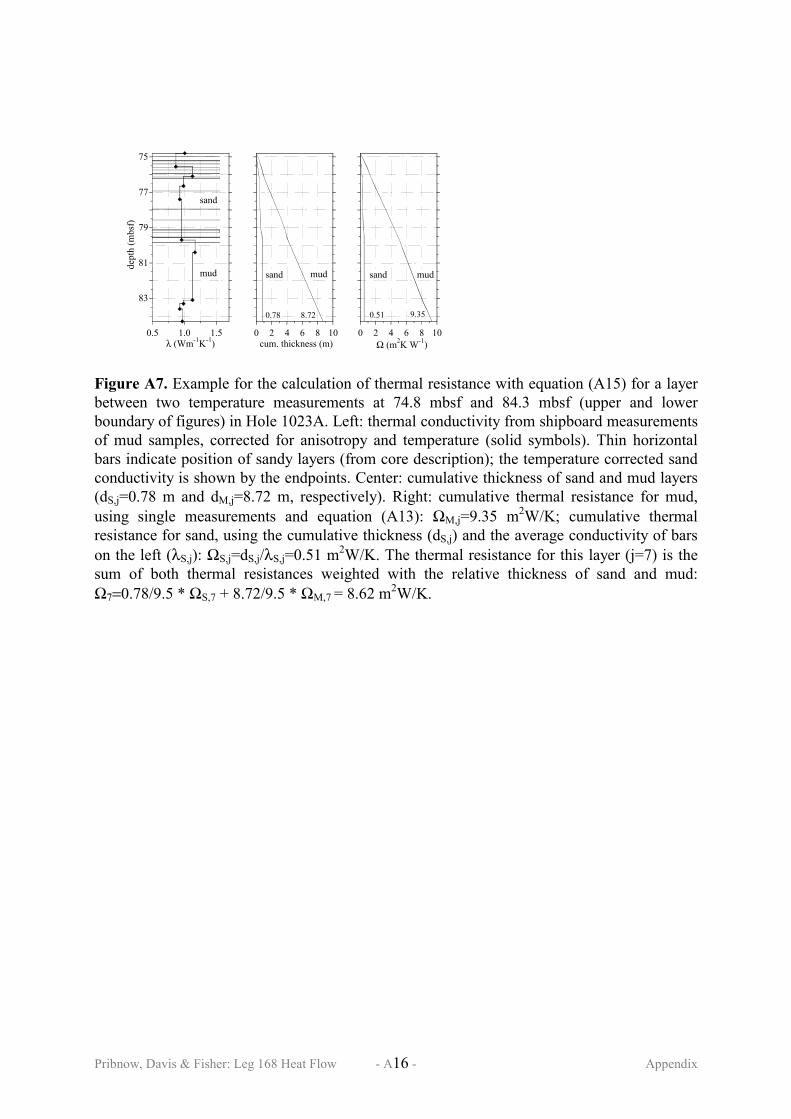
Figure A7. Example for the calculation of thermal resistance with equation (A15) for a layerbetween two temperature measurements at 74.8 mbsf and 84.3 mbsf (upper and lowerboundary of figures) in Hole 1023A. Left: thermal conductivity from shipboard measurementsof mud samples, corrected for anisotropy and temperature (solid symbols). Thin horizontalbars indicate position of sandy layers (from core description); the temperature corrected sandconductivity is shown by the endpoints. Center: cumulative thickness of sand and mud layers(dS,j=0.78 m and dM,j=8.72 m, respectively). Right: cumulative thermal resistance for mud,using single measurements and equation (A13): ΩM,j=9.35 m2W/K; cumulative thermalresistance for sand, using the cumulative thickness (dS,j) and the average conductivity of barson the left (λS,j): ΩS,j=dS,j/λS,j=0.51 m2W/K. The thermal resistance for this layer (j=7) is thesum of both thermal resistances weighted with the relative thickness of sand and mud:Ω7=0.78/9.5 * ΩS,7 + 8.72/9.5 * ΩM,7 = 8.62 m2W/K.

0 2 4 6 8 10Ω (m2K W-1)

sand mud

0.51 9.35

0.5 1.0 1.5

75

77

79

81

83

dept

h (m

bsf)

λ (Wm-1K-1)

sand

mud

0 2 4 6 8 10cum. thickness (m)

sand mud

0.78 8.72

borehole heat flow along the eastern flank of the juan de...

Documents