BoRam: Balancing Robot using Arduino and Lego

Kyungjae Baik (9193618)

September 10, 2008

1

Contents

1 Introduction 3

2 BoRam Description 3

3 System Modeling 43.1 Actuator Assembly Dynamics . . . . . . . . . . . . . . . . . . . . . . . . . . . . . . . . . . . . 43.2 Body Dynamics . . . . . . . . . . . . . . . . . . . . . . . . . . . . . . . . . . . . . . . . . . . . 53.3 System Dynamics . . . . . . . . . . . . . . . . . . . . . . . . . . . . . . . . . . . . . . . . . . . 6

4 Microcontroller 74.1 Arduino . . . . . . . . . . . . . . . . . . . . . . . . . . . . . . . . . . . . . . . . . . . . . . . . 74.2 H-Bridge (Motor Controller) . . . . . . . . . . . . . . . . . . . . . . . . . . . . . . . . . . . . . 7

5 Sensors 85.1 IMU Setup with Kalman Filtering . . . . . . . . . . . . . . . . . . . . . . . . . . . . . . . . . 85.2 Coupling between IMU and Optical Encoder . . . . . . . . . . . . . . . . . . . . . . . . . . . 95.3 Kalman Filtering Code Example . . . . . . . . . . . . . . . . . . . . . . . . . . . . . . . . . . 10

6 Actuator 116.1 Identication of Eective Moment of Inertia . . . . . . . . . . . . . . . . . . . . . . . . . . . . 116.2 Identication of Torque Constant, Choice of PWM Frequency . . . . . . . . . . . . . . . . . . 13

7 Digital Mock-Up 157.1 Parametric Design Technique . . . . . . . . . . . . . . . . . . . . . . . . . . . . . . . . . . . . 157.2 Draft . . . . . . . . . . . . . . . . . . . . . . . . . . . . . . . . . . . . . . . . . . . . . . . . . . 167.3 Applying Physical Properties . . . . . . . . . . . . . . . . . . . . . . . . . . . . . . . . . . . . 16

8 Controller Design 188.1 Digital Controller for Motor Position . . . . . . . . . . . . . . . . . . . . . . . . . . . . . . . . 18

8.1.1 Digital Control - Proportional . . . . . . . . . . . . . . . . . . . . . . . . . . . . . . . . 188.1.2 Digital Control - Root Locus . . . . . . . . . . . . . . . . . . . . . . . . . . . . . . . . 18

8.2 LQR Controller for Balancing . . . . . . . . . . . . . . . . . . . . . . . . . . . . . . . . . . . . 198.2.1 Discrete State-Space . . . . . . . . . . . . . . . . . . . . . . . . . . . . . . . . . . . . . 198.2.2 Controllability . . . . . . . . . . . . . . . . . . . . . . . . . . . . . . . . . . . . . . . . 208.2.3 Digital LQR Full-State Feedback Controller design . . . . . . . . . . . . . . . . . . . . 20

9 Simulation & VRML 21

10 Results and Conclusions 22

11 Reference 24

A Nomenclature 24

B Arduino Conguration 25

C H-Bridge(L293D) Conguration 26

D Physical Properties of BoRam 26

2

The design of a low-cost balancing robot is accomplished by using a popular development platformArduino for the controller and Lego for the construction material. The balancing robot is intended toimprove the learning experience of students or hobbyists who are interested in control theory by presentinghands-on experiments and controller design examples that anyone would be able to follow easily and cost-eectively.

1 Introduction

This paper describes a two-wheel balancing robot which was designed for a project course ENGR6971 undersupervision of Prof. Luis Rodrigues. The kit is based on a popular open-architecture development boardArduino. Arduino uses an ATmega168 chip from Atmel Corporation that runs on a clock speed of 16MHzwith 1KB of SRAM and 16KB of Flash memory. The overall cost of the total kit excluding the Lego partssums around $200 which is well below the cost of similar commercially available educational control kits.The robot is named BoRam in short of Balancing Robot using Arduino and Lego plus some extra letters.The procedure used for system modeling, inertial measurements fusion technique, motor identication, andcontroller design/implementation are described in the following chapters.

2 BoRam Description

Figure 1: Robot Description

BoRam is composed of two stages as illustrated in Figure 1. The bottom stage consists of motors, wheels,and two pairs of spur gears that connect the motors and the wheels. The spur gear was added becausethe motor shaft was not long enough to support the distance required by the optical encoder. The opticalencoder requires some space between the striped disk and the optical sensors to read black and white. Thetop stage consists of a microcontroller and an H-bridge. The microcontroller is the brain of the robot andis responsible to sample and process all the data collected by the sensors. The H-bridge is used with the

3

Part Brand Quantity

Microcontroller Arduino Diecimila 1H-bridge LD293 chip 1DC Motor LEGO Standard Part # 71427 2Encoder Nubotics Optical Encoder 1

Inertial Measurement Unit Sparkfun IMU Combo Board - ADXL203/ADXRS300 1

Table 1: Part list

microcontroller to control the directions of the motors. There is one more sensor attached to a vertical strutbetween the two stages. In general it is called a Inertial Measurement Unit, IMU, and this one contains twoaccelerometers and one gyro to determine the robot's attitude in one angular direction. Table 1 describeswhich part in particular was used in this project.

3 System Modeling

Figure 2: Reference Frame

To make the project simple and manageable, only a two-dimensional movement in which BoRam movesin one plane will be considered. The two motors are assumed to move together symmetrically when anidentical input is given. Although this is unlikely the case, it is a good approximation for motors which aremanufactured as the same product. A control voltage is applied to the motors, which results in displacementof the wheels and change in angular attitude of the body. A mathematical model for the system is obtainedby observing the FBDs in Figure 2.

The rst diagram in Figure 2 indicates the inertial frame. All the equations will be derived in this inertialframe. In the second and third diagram, there are a few variables worthy of clarication. h is the frictionforce between each wheel and surface. H, V are the horizontal and vertical forces acting among the bodyand the motor shaft respectively. l is the length from the motor shaft to the CG of the Body, and nally τis the torque produced by the DC motor.

3.1 Actuator Assembly Dynamics

The observation of the modeling process will start from the third diagram. There are two fundamentalequations describing the characteristics of a DCmotor. The rst one relates torque τ on the shaft proportionalto the armature current i and the second expresses the back emf voltage e proportional to the shaft'srotational velocity ωenc , where ωenc is the velocity measured by the encoder mounted on the same frame asthe DC motor. This velocity represents the shaft velocity with respect to the DC motor itself.

τ = Ki (1)

4

e = Keωenc (2)

The proportionality constant K is called the torque constant, and Ke is called back emf constant.Assume an idealized energy transducer having no power loss in converting electric power into mechanical

power

P = ei = τωenc (3)

Substituting Equation (1) into (3) and dividing both sides by i yields

e = Kωenc (4)

Thus, by comparing Equations (4) and (2) one can conclude that, assuming idealized energy conversion,Ke is identical to K.

BoRam is powered by two Lego 71427 DC motors. Figure 2, third diagram illustrates an electrical circuitin the actuator assembly where Kirchho's voltage law is applied.

v − e−Ri− Ldi

dt= 0 (5)

In deriving the mathematical expression for the motor, shaft viscous friction and inductance are consid-ered negligible to simplify the model. The relative eect of the inductance is negligible compared with themechanical motion and can be neglected.

v − e−Ri = 0 (6)

Applying Newton's law in the third diagram of Figure 2 to the horizontal motion of the wheel, and thento the angular motion induced by two torques yields

mx = h−H (7)

τ − hr = Jω (8)

It is assumed that no slip occurs between the wheels and the surface, so the following relationship musthold.

ω =x

r(9)

ω =x

r(10)

Note that ω is the angular velocity of the wheel in the inertial frame and it is dierent from ωencthat wasused in the DC motor identication section. This will be explained in Section 5.2 Coupling between IMUand optical encoder. It is important to know this relationship especially when it comes to implementing themicrocontroller.

3.2 Body Dynamics

The second diagram in Figure 2 illustrates the body dynamics. The rotational motion of the pendulum bodyabout its center of gravity can be described by

Iθ = −2τ +−2Hl cos θ + 2V l sin θ (11)

where I is the moment of inertia of the pendulum body about its center of gravity. The horizontal force,vertical force and torque are applied as pairs on both sides and each pair is assumed to be equal becauseonly two-dimensional motion was considered.

The horizontal motion is given by

5

2H = Md2

dt2(x+ l sin θ) (12)

The vertical motion is given by

−2V +Mg = Md2

dt2(−l cos θ) (13)

Since BoRam must be kept in a vertical attitude, θcan be assumed to be very small such that sin θ ≈ θ,cos θ = 1. Then, Equations (11) through (13) can be linearized. The linearized equations are

Iθ = −2τ − 2Hl + 2V lθ (14)

2H = M(x+ lθ) (15)

2V = Mg (16)

3.3 System Dynamics

The objective here is to nd suitable ordinary dierential equations that fully describe the system in termsof input v, the states x, θ and their derivatives x, θ. The following describes how to characterize the essenceof the system in two dierential equations.

With Equations (7), (10), and (15) substituted into Equation (8) yields τ in terms of x and θ.

τ =(J

r+ rm+

rM

2

)x+

rMl

2θ (17)

Substituting Equations (3), (1), (9) and (17) into Equation (5) yields

R

K

(J

r+ rm+

rM

2

)x+

RrMl

2Kθ +

K

rx−Kθ = v (18)

Finally substituting Equations (15), (16), (17) into Equation (14) yields

(I + rMl +Ml2

)θ + 2

(J

r+ rm+

rM + lM

2

)x−Mglθ = 0 (19)

Equations (18) and (19) describe the motion of BoRam, and these are the equations that constitute thetwo-dimensional linearized mathematical model of the system. Finally this set of equations can be expressedin a more convenient state-space form as shown in Equation 20.

x

θx

θ

=

0 0 1 00 0 0 10 A32 A33 A34

0 A42 A43 A44

xθx

θ

+

00B3B4

v (20)

The unknown properties, J ,M , m, r, K and R shall be obtained by direct or experimental measurements.Finally I and l shall be found by conducting a full Digital Mock-Up model in CATIA. All of which shall beshown in subsequent chapters.

6

4 Microcontroller

The brain of BoRam is actually two stacks of hardware. The bottom part is Arduino, and what sits on topof this is the motor driver which contains the H-bridge.

Figure 3: The robot main controller assembly

4.1 Arduino1

Arduino is an open-source electronics prototyping platform based on exible, easy-to-use hardware and software. It is originally intended for artists, designers, hobbyists,and anyone interested in creating interactive objects or environments. Because of thisbroad range of users group, the foundation software seems to be somewhat limitedin low-level customizability and extensibility. This comes at a cost of ease of use.However, there are many examples of well-dened coding practice that one could easilyfollow and learn from. Moreover, the software has a long history going back to thefamous even more powerful Wiring platform that had already gone through numerousrevisions proving itself to be reliable.

In this project neither Arduino Foundation Library, nor the editor that came withit was used. Instead GNU C compiler for AVR combined with Eclipse integrated

development environment and Cygwin was used. Some of the codes in Wiring platform came useful butmost of the code was written by myself.

4.2 H-Bridge (Motor Controller)

The L293D is a quadruple high-current half-H driver and is designed to provide bidi-rectional drive currents of up to 600-mA at voltages from 4.5 V to 36 V. It can alsodrive inductive loads such as relays, solenoids, dc and bipolar stepping motors, as wellas other high-current/high-voltage loads in positive-supply applications.

The idea of building this circuit on a Prototype board was originally inspired bythe Motor Controller Shield kit from AdaFruit2 but had been modied for only twoDC motors control, because otherwise, there would be no pins available for othercomponents in BoRam. All hardware schemes in the website are provided with CreativeCommon Licenses, therefore there should be no issues with Copyrights.

1http://www.arduino.cc/2http://ladyada.net/make/mshield/

7

5 Sensors

5.1 IMU Setup with Kalman Filtering

Kalman lter algorithm that was developed by an open-source community3 was adopted and modied. Thealgorithm is part of the autopilot onboard code package. All of the software is free; can be distributed and/ormodied under the terms of the GNU General Public License as published by the Free Software Foundation.

The graphs below illustrate how the Kalman lter can be useful in fusing single-axis angular attitudescollected separately. One way of calculating the attitude is by using two accelerometers. The accelerometerunit gives angular attitude by using arctan2. The orientation ximu, yimu of the IMU is set as ximu pointingto x in inertial frame, but yimu pointing towards −y in inertial frame. Thus to get a θ in accordance to theinertial Equation 21 must hold.

θ = arctan2(x,−y) (21)

The other way of obtaining the attitude is by integrating the angular rate data from the gyro using Eulerintegration. Ideally a jig would be required to provide an absolute reference angle at any given moment,but since the data will only be used as an observational reference and not in the core algorithm itself, it isreasonable to do without a costly jig and roughly compare data from the two sources, accelerometer unitand gyro unit, and ultimately with the Kalman ltering result.

Figure 4: Steady motion measurement using Kalman Filter

Figure 4 is a response to a steady movement. The Y-axis indicates the angle in degrees, and the X-axisis the step count or sampling count from the microcontroller. Usually when implementing a microcontrollera task is programmed to be executed in a routine basis, but in this experiment the microcontroller wasoperated in an endless-loop without any delay time allowing the Euler Integration to produce higher qualityresults. It can be observed that both units reect the angle quite similarly. The experiment was not longenough to catch the drift of the gyro but overall all data seemed to be reliable. So it was necessary to providea harsh environment to intentionally invoke degradation in data. The next experiment was performed in ahard-shaking circumstance.

3http://autopilot.sourceforge.net

8

Figure 5: Unsteady motion measurement using Kalman Filter

Figure 5 shows an interesting result. The IMU board was not only rotated radically but also shakenin order to generate lateral acceleration. The lateral acceleration introduces noise to the system so thatby using accelerometers alone one cannot measure where about the angular attitude is. At the end of theshaking process the gyro reveals an oset compared to the angle provided by the accelerometer. In this caseaccelerometer data is more reliable, and the oset can be considered as an integration propagation error ora continuous drift in angle.

It is very interesting to see that the Kalman lter is following well the patterns of the gyro in a verynoisy environment, whereas, at the end of the shaking process when the sensor is stable, it pertains to themore accurate accelerometer data.

5.2 Coupling between IMU and Optical Encoder

The notation for ω corresponds to the angular velocity of the wheel relative to the inertial frame. The inertialframe was explained in the rst diagram of Figure 2. However what is being measured by the encoder isωenc , and this value is with respect to the Body frame since the encoders are attached to the robot's body.The relationship between ωand ωenccan be described as

ω = ωenc + θ (22)

where θis the angular rate of the Body frame relative to the Inertial frame. Therefore this relationship shouldbe implemented in the microcontroller correctly in order to blend the correct angular velocity in the modeldynamics.

This gives an interesting perspective. The results from two sensors are combined together to give oneresult, in this case, ω. Each sensor has a certain characteristics of its own, it may contain various non-linearfactors such as back-lash, quantization error, or latency but this depends on each individual sensors andbecomes more dicult to lter when the data with dierent kinds of error factors are combined.

The following gure illustrates the data that was collected with the wheels xed at a certain positionand only the body swinging back and forth. The rst 170 steps were performed in a steady slow motionand afterward fast motion was applied to see the dierence. The color green indicates angular rate, ωenc,deduced by the encoder, blue indicates Kalman lter rate, θ, of the body. The color red indicates ω, andin this situation, since the wheels are xed, ω should always be zero. This shows that combining dierentsensor noise factors can introduce signicant noise that is dicult to lter out.

9

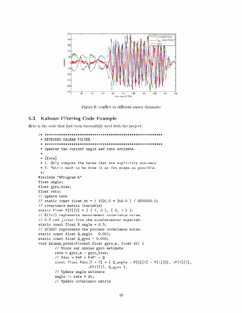
Figure 6: conict in dierent sensor dynamics

5.3 Kalman Filtering Code Example

Here is the code that had been successfully used with the project.

/* *********************************************************

* EXTENDED KALMAN FILTER

* *********************************************************

* Updates the current angle and rate estimate.

*

* [Note]

* 1. Only compute the terms that are explicitly non-zero

* 2. Matrix math to be done in as few steps as possible.

*/

#include "WProgram.h"

float angle;

float gyro_bias;

float rate;

// update rate

// static const float dt = ( 1024.0 * 256.0 ) / 8000000.0;

// covariance matrix (variable)

static float P[2][2] = 1, 0 , 0, 1 ;

// R(1x1) represents measurement covariance noise.

// 0.3 rad jitter from the accelerometer expected.

static const float R_angle = 0.3;

// Q(2x2) represents the process covariance noise.

static const float Q_angle = 0.001;

static const float Q_gyro = 0.003;

void kalman_predict(const float gyro_m, float dt)

// Store our unbias gyro estimate

rate = gyro_m - gyro_bias;

// Pdot = F*P + P*F' + Q

const float Pdot[2 * 2] = Q_angle - P[0][1] - P[1][0], -P[1][1],

-P[1][1], Q_gyro ;

// Update angle estimate

angle += rate * dt;

// Update covariance matrix

10

P[0][0] += Pdot[0] * dt;

P[0][1] += Pdot[1] * dt;

P[1][0] += Pdot[2] * dt;

P[1][1] += Pdot[3] * dt;

void kalman_correct(const float ax_m, const float ay_m)

const float angle_m = atan2(ax_m, -ay_m);

const float angle_err = angle_m - angle;

// The H matrix

const float H_0 = 1;

// PH'

const float PHT_0 = H_0 * P[0][0];

const float PHT_1 = H_0 * P[1][0];

// S = H P H' + R

const float S = R_angle + H_0 * PHT_0;

// K = P H' inv(sS)

const float K_0 =PHT_0 / S;

const float K_1 =PHT_1 / S;

// P = P - K H P

const float HP_0 = PHT_0;

const float HP_1 = H_0 * P[0][1];

P[0][0] -= K_0 * HP_0;

P[0][1] -= K_0 * HP_1;

P[1][0] -= K_1 * HP_0;

P[1][1] -= K_1 * HP_1;

// X += K * err

angle += K_0 * angle_err;

gyro_bias += K_1 * angle_err;

void kalman()

kalman_predict((analogRead(GYRO_PIN) - gyro_zero) * GYRO_SCALE, 0.02);

kalman_correct(analogRead(ACCEL_X_PIN) - ax_zero, analogRead(ACCEL_Y_PIN)

- ay_zero);

6 Actuator

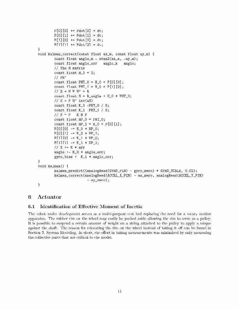
6.1 Identication of Eective Moment of Inertia

The robot under development serves as a multi-purpose test bed replacing the need for a rotary motionapparatus. The rubber tire on the wheel may easily be pushed aside allowing the rim to serve as a pulley.It is possible to suspend a certain amount of weight on a string attached to the pulley to apply a torqueagainst the shaft. The reason for relocating the tire on the wheel instead of taking it o can be found inSection 3. System Modeling. In short, the eort in taking measurements was minimized by only measuringthe collective parts that are critical to the model.

11

Figure 7: FBD of Rotary Motion Apparatus

The experiment of discovering the moment of inertia of all the rotating parts is conducted by droppinga known weight from the pulley. The string may be loosely attached to the pulley so that it can completelyfall o near its end. When the string falls o and when τg no longer exists, the pulley will decelerate andgradually stop due to the constant friction torque τf . Velocity data is collected by the encoder, and theresult is shown in Figure 8.

Figure 8: Rotary motion of the actuator assembly

The graph consists of two constant angular accelerations. The point of switching comes when the stringfalls o from the pulley. The constant deceleration is produced by a constant friction torque τf . Theacceleration torque, τg, is produced by the tension in the string multiplied by r, the moment arm. Thefriction force acts on both cases. The eective moment of inertia J is a result of all the rotating parts,namely, the rotor and reduction gears inside the motor, the wheel, and nally the shaft that connects themall together. The torque produced by the falling weight, τg, can be found by analyzing the tension in thestring while the angular velocity accelerates. According to the second diagram in Figure 7, two equationscan be described as follows.

Jωaccel = τg − τf (23)

mg − τgr

= mrωaccel (24)

12

The relationship in the third diagram in Figure 7 is,

Jωdecel = −τf (25)

There are two equations in which ωaccel, ωdecel, are known and τg can be obtained from Equation (24).Therefore the other two unknowns can be determined easily. Table 2 shows the result.

ωaccel ωdecel τg τf JMotor (Right) 26.039 −3.496 0.0156 0.0019 0.00053

Table 2: Calculation of J and τf using a 0.059[kg] weight and a 0.0293[m] radius pulley

6.2 Identication of Torque Constant, Choice of PWM Frequency

Substituting Equations (1) and (4) into (5) yields

τ =K

Rv − K2

Rωenc (26)

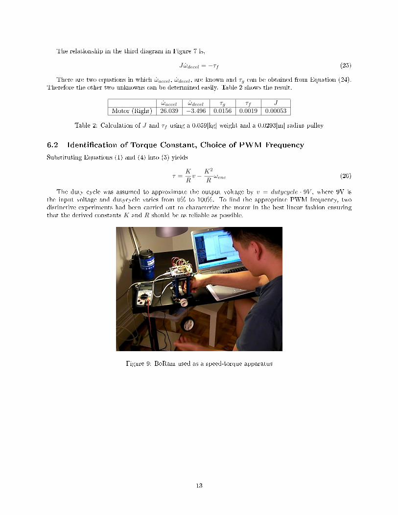
The duty cycle was assumed to approximate the output voltage by v = dutycycle · 9V , where 9V isthe input voltage and dutycycle varies from 0% to 100%. To nd the appropriate PWM frequency, twodistinctive experiments had been carried out to characterize the motor in the best linear fashion ensuringthat the derived constants K and R should be as reliable as possible.

Figure 9: BoRam used as a speed-torque apparatus

13

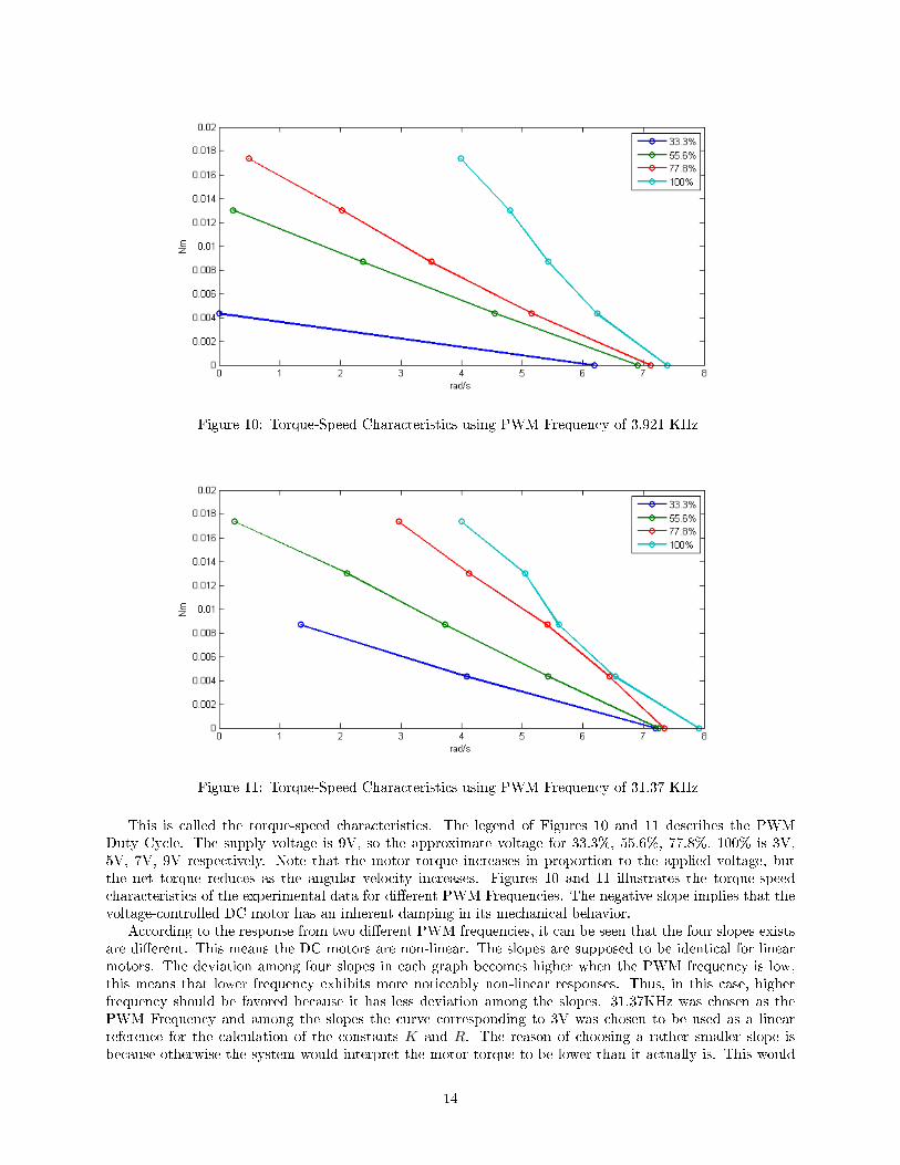
Figure 10: Torque-Speed Characteristics using PWM Frequency of 3.921 KHz

Figure 11: Torque-Speed Characteristics using PWM Frequency of 31.37 KHz

This is called the torque-speed characteristics. The legend of Figures 10 and 11 describes the PWMDuty Cycle. The supply voltage is 9V, so the approximate voltage for 33.3%, 55.6%, 77.8%, 100% is 3V,5V, 7V, 9V respectively. Note that the motor torque increases in proportion to the applied voltage, butthe net torque reduces as the angular velocity increases. Figures 10 and 11 illustrates the torque-speedcharacteristics of the experimental data for dierent PWM Frequencies. The negative slope implies that thevoltage-controlled DC motor has an inherent damping in its mechanical behavior.

According to the response from two dierent PWM frequencies, it can be seen that the four slopes existsare dierent. This means the DC motors are non-linear. The slopes are supposed to be identical for linearmotors. The deviation among four slopes in each graph becomes higher when the PWM frequency is low,this means that lower frequency exhibits more noticeably non-linear responses. Thus, in this case, higherfrequency should be favored because it has less deviation among the slopes. 31.37KHz was chosen as thePWM Frequency and among the slopes the curve corresponding to 3V was chosen to be used as a linearreference for the calculation of the constants K and R. The reason of choosing a rather smaller slope isbecause otherwise the system would interpret the motor torque to be lower than it actually is. This would

14

cause overshoot. By choosing a smaller slope as the reference it may cause slow rise time but overshoot andinstability may be prevented.

PWM Freq K R reference curve3.921 KHz 0.730 272.6Ω 55.6%31.37 KHz 1.0636 290.1Ω 100%31.37 KHz 0.4199 119.1Ω 33.3%

Table 3: Result of Torque-Speed experiment

7 Digital Mock-Up

7.1 Parametric Design Technique

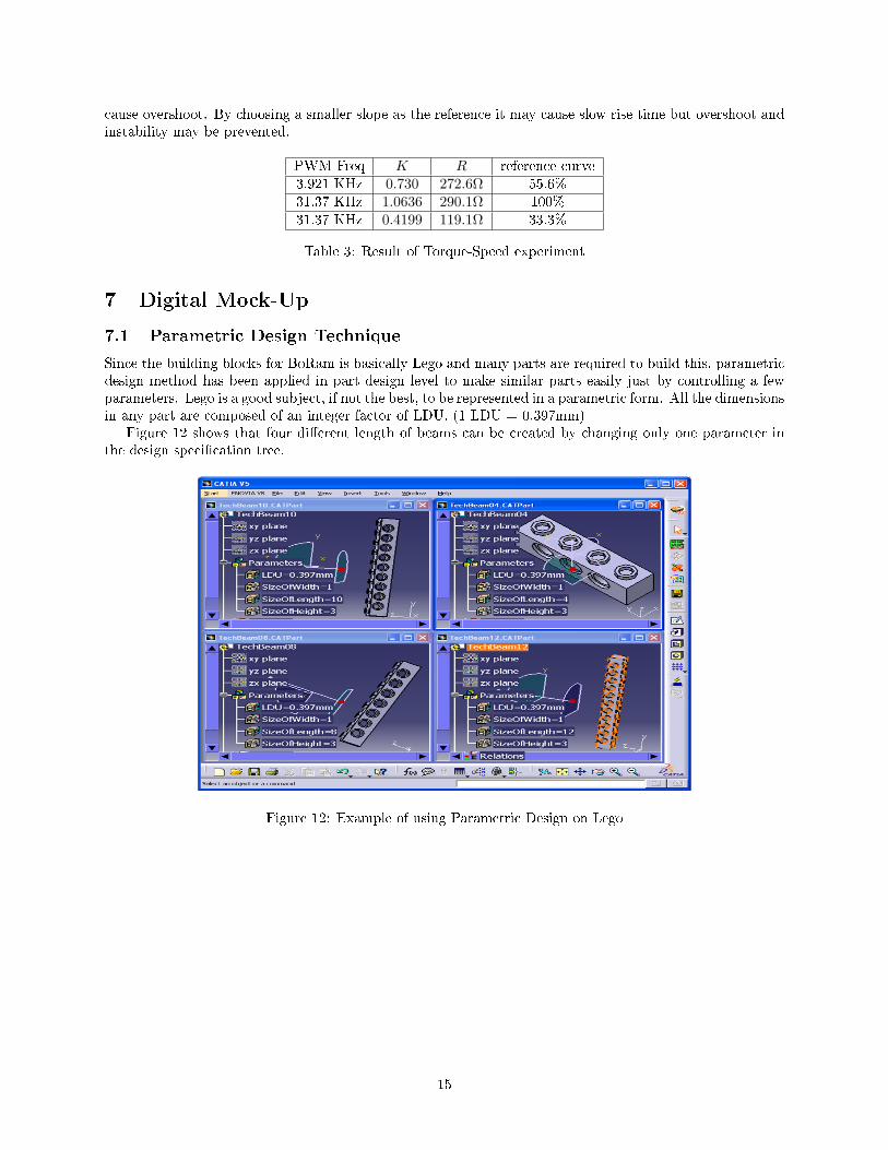
Since the building blocks for BoRam is basically Lego and many parts are required to build this, parametricdesign method has been applied in part design level to make similar parts easily just by controlling a fewparameters. Lego is a good subject, if not the best, to be represented in a parametric form. All the dimensionsin any part are composed of an integer factor of LDU. (1 LDU = 0.397mm)

Figure 12 shows that four dierent length of beams can be created by changing only one parameter inthe design specication tree.

Figure 12: Example of using Parametric Design on Lego

15

7.2 Draft

Figure 13: Example of generating a draft

7.3 Applying Physical Properties

CATIA has a list of supported materials. Lego is known to be made out of ABS plastic, but the closestmaterial to that in CATIA was found to be Plastic. To make a legitimate approximation, important attributesmust match within an acceptable degree. The focus is on static properties, which are essentially mass ormoment of inertia, other properties such as Poisson Ratio and Young Modulus may be neglected. As a resultonly the Specic Gravity should be compared and be similar enough to support the approximation.

It seems that Lego does not ocially disclose information about their material but various web resources

16

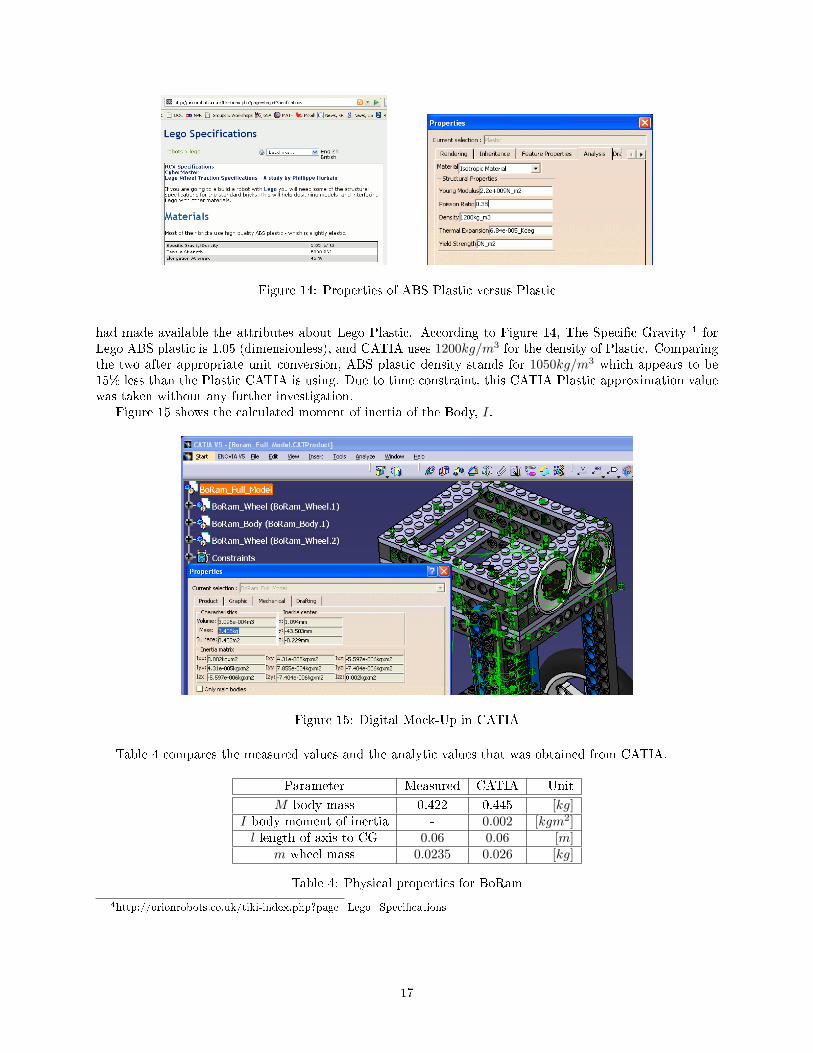
Figure 14: Properties of ABS Plastic versus Plastic

had made available the attributes about Lego Plastic. According to Figure 14, The Specic Gravity 4 forLego ABS plastic is 1.05 (dimensionless), and CATIA uses 1200kg/m3 for the density of Plastic. Comparingthe two after appropriate unit conversion, ABS plastic density stands for 1050kg/m3 which appears to be15% less than the Plastic CATIA is using. Due to time constraint, this CATIA Plastic approximation valuewas taken without any further investigation.

Figure 15 shows the calculated moment of inertia of the Body, I.

Figure 15: Digital Mock-Up in CATIA

Table 4 compares the measured values and the analytic values that was obtained from CATIA.

Parameter Measured CATIA Unit

M body mass 0.422 0.445 [kg]I body moment of inertia - 0.002 [kgm2]l length of axis to CG 0.06 0.06 [m]

m wheel mass 0.0235 0.026 [kg]

Table 4: Physical properties for BoRam

4http://orionrobots.co.uk/tiki-index.php?page=Lego+Specications

17

8 Controller Design

8.1 Digital Controller for Motor Position

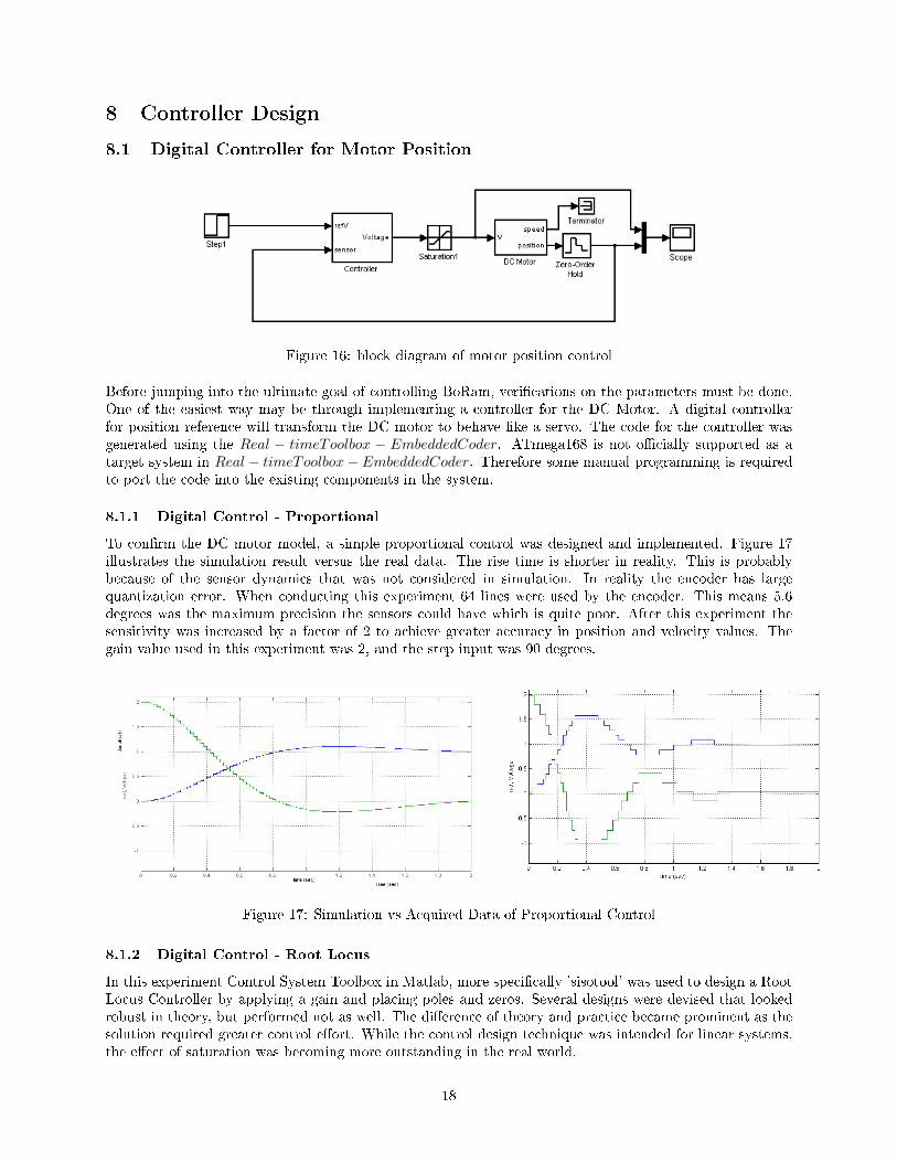
Figure 16: block diagram of motor position control

Before jumping into the ultimate goal of controlling BoRam, verications on the parameters must be done.One of the easiest way may be through implementing a controller for the DC Motor. A digital controllerfor position reference will transform the DC motor to behave like a servo. The code for the controller wasgenerated using the Real − timeToolbox − EmbeddedCoder. ATmega168 is not ocially supported as atarget system in Real − timeToolbox− EmbeddedCoder. Therefore some manual programming is requiredto port the code into the existing components in the system.

8.1.1 Digital Control - Proportional

To conrm the DC motor model, a simple proportional control was designed and implemented. Figure 17illustrates the simulation result versus the real data. The rise time is shorter in reality. This is probablybecause of the sensor dynamics that was not considered in simulation. In reality the encoder has largequantization error. When conducting this experiment 64 lines were used by the encoder. This means 5.6degrees was the maximum precision the sensors could have which is quite poor. After this experiment thesensitivity was increased by a factor of 2 to achieve greater accuracy in position and velocity values. Thegain value used in this experiment was 2, and the step input was 90 degrees.

Figure 17: Simulation vs Acquired Data of Proportional Control

8.1.2 Digital Control - Root Locus

In this experiment Control System Toolbox in Matlab, more specically 'sisotool' was used to design a RootLocus Controller by applying a gain and placing poles and zeros. Several designs were devised that lookedrobust in theory, but performed not as well. The dierence of theory and practice became prominent as thesolution required greater control eort. While the control design technique was intended for linear systems,the eect of saturation was becoming more outstanding in the real world.

18

One of the working design is presented. The control eort was designed to be kept below the saturationpoint, however the same quantization error that occurred in Proportional Control experiment was alsoobservable here as well.

Figure 18: Root Locus Design

Parameter Value

Gain 7.26864330434832Zeros [-0.973326359832636;0.90376569037657]Poles [0.71;-0.98]

Controller =7.2686(z + 0.9733)(z − 0.9038)

(z − 0.71)(z + 0.98)

Figure 19: Simulation vs Acquired Data of Root Locus Design

8.2 LQR Controller for Balancing

8.2.1 Discrete State-Space

To obtain a discrete model of the system, rst one must nd the state-space representation in continuous-time domain and then convert it to discrete domain. In this case a conversion method called zero-order hold

19

was used. It is a common practice to have 25~30 times of the bandwidth frequency of the closed-loop systemas the sampling time but there is another constraint that needs to be considered, which is the processingpower of the microcontroller. Not knowing exactly the bandwidth, 0.02[s] was chosen as the sampling timeout of a random pick. It should be observed whether the microcontroller is capable of processing the datawithout being over-run. Since the microcontroller has a limited amount of resource, reducing the period ofsampling time can be achieved by trial and error until the microcontroller begins to over-run and fail.

The two linearized ordinary dierential Equations (18), (19) representing the system can be modeledin Simulink as shown below. Although having a non-linear system model for the simulation andusing the linearized model for linear controller design is a recommended practice, howevertime was not allowed to model a non-linear model within Simulink.

Figure 20: linearized system model

8.2.2 Controllability

The design criteria for the system was simply to make BoRam balance permanently. Criteria for settlingtime, rise time, overshoot and steady-state error were just too much for the initial controller design phase.Moreover, having done a rough linearization on highly non-linear toy parts and the lack of mental convictionof the possibility of ne tuning had also contributed to settling down on a rather simplied goal.

In theory, there is a way to gain assurance on whether a system is controllable or not. For the systemto be completely state controllable, the controllability matrix must have the rank of n. Consider the lineartime invariant system given by

x = Ax+Bu

The controllability matrix of the above LTI system is dened by the pair (A,B) as follows

Cr(A,B) = [B,AB,A2B,A3B]

The rank of the matrix is the number of independent rows. Applying this condition to our model gave 4.Thus the system is controllable! This proves that the current discrete system is completely state controllable.

8.2.3 Digital LQR Full-State Feedback Controller design

The next step and the most critical step is to nd the control matrix(K). The linear quadratic regulatormethod is used to nd the control matrix. This method allows to nd the optimal control matrix thatresults in some balance between system errors and control eort. To use LQR method, three parametersshould be found: Performance index matrix(R), state-cost matrix(Q), and weighting factors. For the sake ofsimplicity, performance index matrix shall be equal to 1. The weighting factor shall be chosen by trial anderror. Finally the control input shall be a step input of 0.2[m].

20

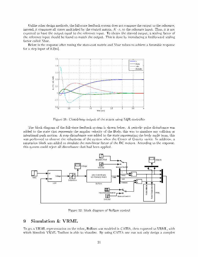
Unlike other design methods, the full-state feedback system does not compare the output to the reference,instead, it compares all states multiplied by the control matrix, K · x, to the reference input. Thus, it is notexpected to have the output equal to the reference input. To obtain the desired output, a scaling factor ofthe reference input should be found to match the output. This is done by introducing a feedforward scalingfactor called Nbar.

Below is the response after tuning the state-cost matrix and Nbar values to achieve a favorable responsefor a step input of 0.2[m].

Figure 21: Closed-loop output of the states using LQR controller

The block diagram of the full-state feedback system is shown below. A periodic pulse disturbance wasadded to the state that represents the angular velocity of the Body, this was to simulate any collision orintentional push motion. A step disturbance was added to the state representing the body angle term, thiswas performed to observe the robustness of the system when the Center of Gravity varies. In addition, asaturation block was added to simulate the non-linear factor of the DC motors. According to the response,this system could reject all disturbance that had been applied.

Figure 22: block diagram of BoRam control

9 Simulation & VRML

To get a VRML representation on the robot, BoRam was modeled in CATIA, then exported to VRML, withwhich Simulink VRML Toolbox is able to visualize. By using CATIA one can not only design a complex

21

model quite easily but also apply physical material properties to the individual parts and get informationregarding CG, or moment of inertia of the full assembly.

Due to the amount of details of the VRML model the real-time rendering was tediously slow, so anothersimplied model was designed for testing purposes. The testing procedure includes dening joints andcoinciding coordinate systems. After all is well working the simplied model is swapped to the complexmodel, then by using the video recording option in VRML Toolbox the simulation can be recorded and canbe viewed smoothly.

Figure 23: block diagram for VRML simulation

Figure 24: simplied VRML Model v.s. complex VRML Model

10 Results and Conclusions

Figure 25 illustrates two scope graphs as a result of the Simulation. The scope on the top shows the outputstates; x in yellow and θ in pink, the one on the bottom shows the input voltage to the motors. These areresults of a step input of 20cm starting at 1 sec, then when the time-line reaches 0:02, a periodic impulse inangular velocity is added to the body with magnitude of 0.1 rad/s, width of 0.2 seconds, for every 2 seconds.Finally a change in attitude to the body angle, 0.1 rad is added to mimic the change in CG. The result wasa success in terms of stability.

22

Figure 25: Scope graph

The next step after a satisfactory in simulation will be, of course, putting BoRam into a real test. Therobot was able to balance for as long as possible while being able to reject mild disturbance applied bypushing the robot back and forth. Figure 26 illustrates BoRam in action.

Figure 26: BoRam in Action

BoRam was built thoroughly by using toy parts and hobbyist-graded parts which are inexpensive com-pared to industrial parts. The quality dierence was observed in the non-linearity and the quantization error

23

characteristics that had been carried out in this project. In spite of massive assumptions on linearity andneglecting many hard-to-dene parameters, the control algorithm that was applied seemed to work ne. Thisproves the robustness of the systematic approach that was taken to solve this control problem and opens awide possibility that one can achieve even more with less.

11 Reference

• Franklin, Gene F.,Powell, J. D. and Emami-Naeini, Abbas. Feedback control of dynamic systems 2006

• Ogata, Katsuhiko. Modern control engineering

• Mohinder S. Grewal, Angus P. Andrews, Kalman Filtering: Theory and Practice Using Matlab

• IEEE Transaction on Industrial Electronics, Vol. 49, No. 1, Feb 2002, JOE: A Mobile, InvertedPendulum

• Tim Wescott, Applied Control Theory for Embedded Systems

• H. Harry Asada, Department of Engineering, MIT, Introduction to Robotics

• Experiment09: Angular Momentum, Physics Department, MIT, 2003

• www.library.cmu.edu/ctms

• www.arduino.cc

• www.wiring.org.co

• www.geology.smu.edu/~dpa-www/robo/nbot/index.html

• www.nongnu.org/avr-libc

• autopilot.sourceforge.net

A Nomenclature

attributes SI unit

M - mass of the body kgm - mass of the wheels kgJ - moment of inertia of the actuator assembly kg ·m2

I - moment of inertia of the body kg ·m2

τ - torque generated from the motor's armature N ·me - back emf voltage VR - DC motor windings resistance ΩK - torque constant N ·m

A

Ke - back emf constant Vrad·s

ω - wheel velocity in reference frame rads

ω - wheel acceleration in reference frame rads2

ωenc- wheel velocity from encoder (body frame) rads

h - friction force Nr - wheel radius mH - horizontal force between body and wheel NV - vertical force between body and wheel N

Table 5: Nomenclature

24

B Arduino Conguration

ATmega168 pin port function Arduino pin interface

1 PC6 RESET RESET R2 PD0 RXD D00(RX) R3 PD1 TXD D01(TX) R4 PD2 INT0 D02 ENCODER_2A5 PD3 OC2B/INT1 D03 ENCODER_1A6 PD4 D04 L293/027 VCC VCC R8 GND GND R9 PB6 CRYSTAL R10 PB7 CRYSTAL R11 PD5 OC0B D05 L293/0112 PD6 OC0A D06 L293/0913 PD7 D07 L293/1014 PB0 D08 L293/1515 PB1 OC1A D09 L293/0716 PB2 OC1B D10 ENCODER_2B17 PB3 OC2A D11 ENCODER_1B18 PB4 D1219 PB5 D13 DEBUG LED20 AVCC VCC 5V21 AREF AREF22 GND GND GND23 PC0 ADC0 A00 2.5REF24 PC1 ADC1 A01 ACCEL X25 PC2 ADC2 A02 ACCEL Y26 PC3 ADC3 A03 GYRO27 PC4 ADC4 A04 POT28 PC5 ADC5 A05

Table 6: Arduino pin mapping

Summary of Arduino specication:

Microcontroller ATMega168Operating Voltage 5V

Input Voltage (recommended) 7~12VDigital I/O Pins 14 (including 6 PWM outputs)Analog Input Pins 6 (10bit ADC)

DC Current per I/O Pin 40mADC Current for 3.3V Pin 50mA

Flash Memory 16KBSRAM 1KB

EEPROM 512 bytesClock Speed 16MHz

25

C H-Bridge(L293D) Conguration

LD293 pin port interface description

1 1,2EN ARDUINO/D05 MOTOR1PWM2 1A ARDUINO/D04 MOTOR_1A3 1Y MOTOR1_RED4 HSK/GND5 HSK/GND6 2Y MOTOR1_BLK7 2A ARDUINO/D09 MOTOR_1B8 VCC2 9V EXTERAL9 3,4EN ARDUINO/D06 MOTOR2PWM10 3A ARDUINO/D07 MOTOR_2A11 3Y MOTOR2_RED12 HSK/GND13 HSK/GND14 4Y MOTOR2_BLK15 4A ARDUINO/D08 MOTOR_2B16 VCC1 5V INTERNAL

Table 7: H-Bridge pin mapping

D Physical Properties of BoRam

Param Measured Catia Unit

M 0.418 (body w/ electronics) + 0.044 (battery) 0.353 (body w/o electronics) [kg]I - 0.002 [kgm2]l 0.06 0.06 [m]m 0.0295 0.026 [kg]r 0.041 0.041 [m]

Table 8: Physical properties for BoRam

mass gear ratio

42 [g] 13.2583 : 1

Table 9: Lego Motor 71427 Specication

26