Bootstrap Re�nements for QML Estimators of the GARCH(1,1)

Parameters

Valentina corradi �z

University of Warwick

Emma M. Iglesiasyz

Michigan State University

This draft: April 18, 2007

Abstract

This paper reconsiders a block bootstrap procedure for Quasi Maximum Likelihood esti-

mation of GARCH models, based on the resampling of the likelihood function, as proposed by

Gonçalves and White (2004). First, we provide necessary conditions, in terms of moments of the

innovation process, for the existence of the Edgeworth expansion of the GARCH(1,1) estimator,

up to the k�th term . Second, we provide su¢ cient conditions for higher order re�nements

for equally tailed and symmetric test statistics. In particular, the bootstrap estimator based

on resampling the likelihood has the same higher order improvements in terms of error in the

rejection probabilities as those in Andrews (2002).

Keywords: block bootstrap, Edgeworth expansion, higher order re�nements, Quasi Maximum

Likelihood, GARCH.

�Valentina Corradi, Department of Economics, University of Warwick, Coventry CV4 7AL, UK. e-mail: vcor-

radi@warwick.ac.uk.yEmma Iglesias, Department of Economics, Michigan State University, 101 Marshall-Adams Hall, East Lansing,

MI 48824-1038, USA. e-mail: iglesia5@msu.edu.zBoth authors thank the �nancial support from an ESRC grant (Award number: T026 27 1238) and Intramural

Research Grants Program (IRGP) at Michigan State University. Corradi also gratefully acknowledge �nancial support

from ESRC grant code RES-062-23-0311. We also wish to thank Silvia Gonçalves, Lutz Kilian and Tim Vogelsang for

very useful comments and suggestions.

1

1 Introduction

It is well known that the quasi likelihood function of a GARCH (Generalized Autoregressive Condi-

tional Heteroskedasticity) model, introduced by Bollerslev (1986), depends on the entire past history

of the observables. In this case, resampling blocks of observations is not equivalent to resampling

blocks of the likelihood function. This point has been lucidly pointed out by Gonçalves and White

(2004), who indeed suggest to construct bootstrap estimators of GARCHmodels based on resampling

blocks of the likelihood function. We go a step further, and we investigate the higher order properties

of such estimators. This is accomplished in two steps. First, we establish the necessary conditions

for the existence of an Edgeworth expansion up to the k�th term. This collapses to the existence ofa minimum number of moments of the innovation process. Second, we provide su¢ cient conditions

for higher order improvements of equally tailed and symmetric t-tests based on Quasi Maximum

Likelihood Estimators (QMLE) of GARCH(1,1) processes. This is done by providing the su¢ cient

number of moments of the innovation process needed for the moments of the actual and bootstrap

statistics to approach each other at an appropriate rate. Broadly speaking, this allows to control the

rate at which the di¤erence between the Edgeworth expansion of the actual and bootstrap statistic

approaches zero. Thereafter, we can proceed along the same lines of Andrews (2002). Linton (1997)

calculated the Edgeworth-B distribution function for the GARCH(1,1), and we extend his setting to

the Edgeworth expansion in the context of the existence of re�nements of the bootstrap.

In nutshell, we need (i) conditions on the parameter space of the process in order to ensure

that the GARCH process is exponentially ��mixing (see e.g. Carrasco and Chen (2002)), (ii) theGötze and Hipp (1994) conditions for the existence of the Edgeworth expansion for weakly dependent

observations (iii) the existence of a given number of moments of the innovation process, in order to

obtain the same higher order re�nement of Andrews (2002). Thus, the block bootstrap based on

resampling the likelihood, leads to error in rejection probability and con�dence interval coverage

probability of smaller order than T�1=2�� for equally tailed t-tests for GARCH parameters and of

order smaller than T�1�� for symmetric t-tests, for � > 0; and such that � < and � + < 1=2;

where is the parameter controlling the lengths of the block l; i.e. l ' T :Needless to say, an advantage of using bootstrap estimators is that of obtaining more accurate

inference on the GARCH(1,1) parameters. Gonçalves and Kilian (2004, 2007) focused on bootstrap

inference for conditional mean that is robust to GARCH or other unspeci�ed forms of conditional

heteroskedasticity. However, there are many cases in practice where we are interested on the GARCH

parameters themselves. Nevertheless, from a more empirical perspective, one of the most popular

application of bootstrap estimation of GARCH parameters is in the context of risk management, and

more precisely in the evaluation of Value at Risk and Expected Shortfall. For example, Christof-

2

fersen and Gonçalves (2005) rely on bootstrapping GARCH parameters in order to take into proper

consideration the contribution of parameter estimation error when evaluating Value at Risk; Mancini

and Trojani (2005) address the same issue using an estimation and bootstrap procedure robust to the

presence of outliers. Both papers rely on the residual based bootstrap approach outlined by Pascual,

Romo and Ruiz (2006).

If one knew the data generating process (DGP), then a residual based bootstrap approach, which

makes direct use of the structure of the model, seems to be more natural than a nonparametric

bootstrap approach, such as the block bootstrap. Nevertheless, to the best of our knowledge, the

�rst order validity of the residual-based bootstrap for GARCH models has not yet been proved.1

We have attempted to do this. However, though we do not claim that the residual based bootstrap

is �rst order invalid, our conjecture goes in this direction. In fact, we note that the bootstrap Hessian

cannot properly mimic the sample Hessian, as the moment of the former does not necessarily approach

the moment of the latter. Not surprisingly this is due to the fact that the conditional variance process

is highly nonlinear and depends on the entire history of the past.

In the case of possible nonlinear Markov processes, recent papers by Andrews (2005) and Horowitz

(2003) have established that high order re�nements, very close to those attainable in the iid case, can

be achieved via the use of the Markov bootstrap, even in the case the underlying transition density

is unknown, and replaced by a nonparametric estimator. Though a GARCH process is not Markov,

under certain conditions is approximate Markov, as in the de�nition of Horowitz. Thus, we have

analyzed the applicability of the Markov process as for the estimation of the conditional variance

parameters. It turns out, the Markov bootstrap is valid and outperforms �rst order asymptotics,

only if the marginal density of the innovation process is known.

The rest of this paper is organized as follows. Section 2 describes the implementation of the

bootstrap procedure based on the resampling of the likelihood function. Section 3 establishes the

higher order improvement of the bootstrap GARCH, and summarizes the main theoretical results.

Section 4 outlines several pitfalls which may occur with the residual-based bootstrap for GARCH.

Section 5 outlines pitfalls in the use of the Markov bootstrap, whenever the marginal density of

the innovation is unknown. Section 5 reports Monte Carlo simulation results, which provide some

evidence of the improved accuracy of bootstrap, as for the error in the coverage probability. All the

proofs are collected in the Appendix.

1Hidalgo and Za¤aroni (2007) indeed show the �rst order validity for ARCH(1); characterized by a particulardecay in the ARCH order.

3

2 The Block Bootstrap: Set-Up

Suppose yt is generated by the GARCH(1,1) process,

(1) yt =pht�t; ht = �

y1 + �

y2y2t�1 + �

y3ht�1; t = 1; :::; T

where �t is iid and �y =

��y1; �

y2; �

y3

�is the true parameter vector.

We de�ne the log-likelihood function as if ytphtwere normally distributed, thus using a Gaussian

likelihood. The quasi maximum likelihood estimator, QMLE, is then de�ned as:

(2) b�T = argmax�2�

1

T

TXt=1

Lt (�)

where1

T

TXt=1

Lt (�) = �1

2

TXt=1

lnht(�)�1

2

TXt=1

y2tht (�)

:

Note that after a few manipulations, and imposing h0 = �0 = 0; we have that2

ht = �1 +��2�

2t�1 + �3

�ht�1

= �1

"1 +

t�1Xj=1

jYi=1

��2�

2t�i + �3

�#:(3)

From (3) it is immediate to see that resampling blocks of the observable series yt is not equivalent

to resampling blocks of the log-likelihood.

Thus, we need to resample b blocks of length l from the loglikelihood Lt; setting bl = T: Hereafter, let

Ii; i = 1; :::; b denote identical and independent draws from a discrete uniform on 0; 1; :::; T � l: Thus,for each i = 1; ::; b Ii = j, with j = 0; 1; :::; T�l; with equal probability 1=(T�l+1):Now, for all � 2 �;de�ne L�1 (�) ; L

�2 (�) ; :::; L

�T�l+1 (�) ; :::; L

�T (�) to be equal to LI1+1 (�) ; LI1+2 (�) ; ::::; LIb+1 (�) ; :::; LI1+l (�) :

Note, that we use the same random draws Ii for any � 2 �: In general, resampling the data or re-sampling the likelihood is equivalent. However, in the GARCH case, the (quasi) likelihood function

depends on the entire past history of the observables. In this case, resampling blocks of observa-

tions is not equivalent to resampling blocks of the likelihood function. This point has been lucidly

pointed out by Gonçalves and White (2004), who indeed suggest to construct bootstrap estimators

of GARCH model based on resampling blocks of the likelihood function. We use the moving blocks

bootstrap (MBB) of Künsch (1989) as in Gonçalves and White (2004).

It should be pointed out that, if we were just interested in �rst order validity, then we could have

set l = 1 and rely on the iid nonparametric bootstrap. In fact, as the score is a martingale di¤erence

2Note that if either h0 or �0 are di¤erent from zero, then the expression in (3) holds up to a term converging to

zero exponentially as t!1:

4

sequence, bootstrap samples based on iid resampling of the log-likelihood would have ensured that

the �rst two bootstrap moments properly mimic the correspondent sample moments. However, as

for re�nements, we need to match higher moments, and in this case the fact that the score is a

martingale di¤erence sequence does not help.

We now use the resample log-likelihood in order to construct the bootstrap estimator b��T , that is:b��T = argmax

�2�

1

T

TXt=1

�L�t (�)�

�E��rL�t (b�T )��0 �� :

Note that the recentering term,�E��rL�t (b�T )��0 �; ensure that the score, evaluated at b�T ; has zero

mean.

De�ne the Hessian and the variance of the score as By and Ay respectively, where

By = E��r2

�Lt(�y)�

and

Ay = V ar

1pT

TXt=1

r�Lt(�y)

!= E

�r�Lt(�

y)r�Lt(�y)0�:

Also, de�ne the sample analogs of By and Ay; that is

bBT = � 1T

TXt=1

r2�Lt(

b�T )

(4) bAT = 1

T

TXt=1

r�Lt(b�T )r�Lt(b�T )0:Our objective is to provide higher order re�nements for the t-statistic

(5) t�i;T =� bB�1 bA bB�1��1=2

ii

�b�i;T � �yi� ;for i = 1; 2; 3:

De�ne the bootstrap analogs of bBT and bAT as bB�T and bA�T ; wherebB�T = 1

T

TXt=1

r�rL�t (b�T )� E� �rL�t (b�T )��

and

(6) bA�T = 1

T

TXt=1

�rL�t (b�T )� E� �rL�t (b�T )���rL�t (b�T )� E� �rL�t (b�T )��0 :

5

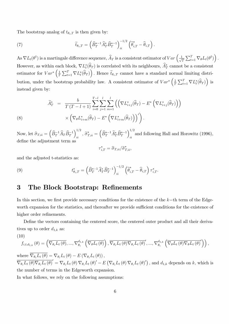
The bootstrap analog of t�i;T is then given by:

(7) et�i;T = � bB��1TbA�T bB��1T

��1=2ii

�b��i;T � b�i;T� :AsrLt(�y) is a martingale di¤erence sequence, bAT is a consistent estimator of V ar � 1p

T

PTt=1r�Lt(�

y)�:

However, as within each block, rL�t (b�T ) is correlated with its neighbours, bA�T cannot be a consistentestimator for V ar�

�1T

PTt=1rL�t (b�T )� : Hence et�i;T cannot have a standard normal limiting distri-

bution, under the bootstrap probability law. A consistent estimator of V ar��1T

PTt=1rL�t (b�T )� is

instead given by:

eA�T =b

T (T � l + 1)

T�lXi=0

lXj=1

lXm=1

��rL�i+j(b�T )� E� �rL�i+j(b�T )��

��r�L

�i+m(

b�T )� E� �rL�i+m(b�T )��0� :(8)

Now, let b�T;ii = � bB�1T bAT bB�1T �1=2ii; e��T;ii = � bB��1T

eA�T bB��1T

�1=2iiand following Hall and Horowitz (1996),

de�ne the adjustment term as

� �i;T = b�T;ii=e��T;ii;and the adjusted t-statistics as:

(9) t��i;T =� bB��1T

bA�T bB��1T

��1=2ii

�b��i;T � b�i;T� � �i;T :3 The Block Bootstrap: Re�nements

In this section, we �rst provide necessary conditions for the existence of the k�th term of the Edge-

worth expansion for the statistics, and thereafter we provide su¢ cient conditions for the existence of

higher order re�nements.

De�ne the vectors containing the centered score, the centered outer product and all their deriva-

tives up to order d1;k as:

(10)

fi;t;d1;k (�) =�r�iLt (�); :::;r

d1;k�i

�r�Lt (�)

�;r�iLt (�)r�iLt (�)

0; :::;rd1;k

�i

�r�Lt (�)r�Lt (�)

0��;

where r�iLt (�) = r�iLt (�)� E (r�iLt (�)) ;

r�iLt (�)r�iLt (�)0= r�iLt (�)r�iLt (�)

0�E�r�iLt (�)r�iLt (�)

0� ; and d1;k depends on k; which isthe number of terms in the Edgeworth expansion.

In what follows, we rely on the following assumptions:

6

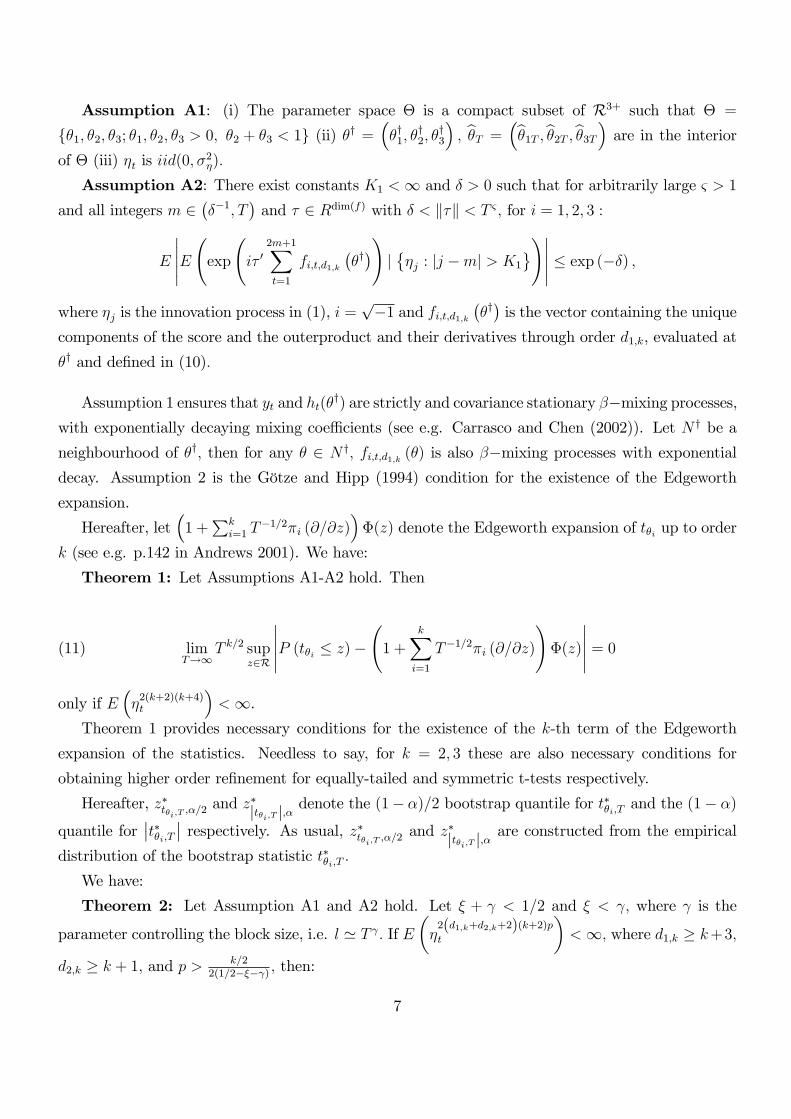
Assumption A1: (i) The parameter space � is a compact subset of R3+ such that � =

f�1; �2; �3; �1; �2; �3 > 0; �2 + �3 < 1g (ii) �y =��y1; �

y2; �

y3

�; b�T = �b�1T ;b�2T ;b�3T� are in the interior

of � (iii) �t is iid(0; �2�):

Assumption A2: There exist constants K1 <1 and � > 0 such that for arbitrarily large & > 1

and all integers m 2���1; T

�and � 2 Rdim(f) with � < k�k < T & ; for i = 1; 2; 3 :

E

�����E exp

i� 0

2m+1Xt=1

fi;t;d1;k��y�!j��j : jj �mj > K1

!����� � exp (��) ;where �j is the innovation process in (1), i =

p�1 and fi;t;d1;k

��y�is the vector containing the unique

components of the score and the outerproduct and their derivatives through order d1;k, evaluated at

�y and de�ned in (10):

Assumption 1 ensures that yt and ht(�y) are strictly and covariance stationary ��mixing processes,

with exponentially decaying mixing coe¢ cients (see e.g. Carrasco and Chen (2002)). Let N y be a

neighbourhood of �y; then for any � 2 N y; fi;t;d1;k (�) is also ��mixing processes with exponentialdecay. Assumption 2 is the Götze and Hipp (1994) condition for the existence of the Edgeworth

expansion.

Hereafter, let�1 +

Pki=1 T

�1=2�i (@=@z)��(z) denote the Edgeworth expansion of t�i up to order

k (see e.g. p.142 in Andrews 2001). We have:

Theorem 1: Let Assumptions A1-A2 hold. Then

(11) limT!1

T k=2 supz2R

�����P (t�i � z)� 1 +

kXi=1

T�1=2�i (@=@z)

!�(z)

����� = 0only if E

��2(k+2)(k+4)t

�<1.

Theorem 1 provides necessary conditions for the existence of the k-th term of the Edgeworth

expansion of the statistics. Needless to say, for k = 2; 3 these are also necessary conditions for

obtaining higher order re�nement for equally-tailed and symmetric t-tests respectively.

Hereafter, z�t�i;T ;�=2and z�jt�i;T j;�

denote the (1� �)=2 bootstrap quantile for t��i;T and the (1� �)quantile for

��t��i;T �� respectively. As usual, z�t�i;T ;�=2 and z�jt�i;T j;� are constructed from the empirical

distribution of the bootstrap statistic t��i;T :

We have:

Theorem 2: Let Assumption A1 and A2 hold. Let � + < 1=2 and � < ; where is the

parameter controlling the block size, i.e. l ' T : If E��2(d1;k+d2;k+2)(k+2)pt

�<1; where d1;k � k+3;

d2;k � k + 1; and p > k=22(1=2��� ) ; then:

7

(i) for k = 2;

P�t�i;T < �z�t�i;T ;�=2 or t�i;T > z

�t�i;T ;�=2

�= �+ o

�T�(1=2+�)

�(ii) for k = 3;

P�jt�i;T j < z�jt�i;T j;�

�= �+ o

�T�(1+�)

�:

From Theorem 2, it is immediate to say that we obtain the same higher order re�nements for the

error in rejection probability (ERP), as in Andrews (2002). As an immediate corollary, we also have

that the bootstrap error in the coverage probability (ECP) is also of order smaller than T�(1=2+�) for

equally tailed test and of T�(1+�) for symmetric test, with � < 1=4: It is interesting to note that, in

the exponentially mixing GARCH(1,1) case, the only condition we need for higher order re�nements

is in terms of existence of a su¢ cient number of moments of the innovation process.

4 The Residual-Based Bootstrap

The residual-based bootstrap is based on iid resampling of the centered residuals. Let b�t = yt=rht �b�T�;where b�T is the QML estimator de�ned in (2). Thus, we resample, with replacement, from the empir-ical distribution of b�t; and obtain the sequence b��t ; where ��1 is equal to b�t� T�1PT

t=1 b�t; t = 1; :::; Twith equal probability 1=T: ��1; �

�2; :::; �

�T are de�ned analogously, so that �

�t ; is iid conditional on

sample. We then proceed as follows:

Fix y0; h0, =) bh�1 = b�1;T + b�2;Ty20 + b�3;Th0y�1 =

qbh�1��1bh�2 = b�1;T + b�2;Ty2�1 + b�3;Tbh�1y�2 =

qbh�2��2and so on, until sequences y�t ; h

�t ; t = 1; :::; T are formed.

Now, de�ne the bootstrap QML estimator as:

(12) e��T = argmax�2�

TXt=1

L�(RS)t (�) = argmax

�2�

�12

TXt=1

lnh�t (�)�1

2

TXt=1

y�2th�t (�)

!;

where the superscript (RS) denotes the fact that the bootstrap likelihood is based on the residual

bootstrap approach. This residual based bootstrap procedure has been recently suggested by Pascual,

Romo and Ruiz (2003). See also Christo¤ersen and Gonçalves (2005), for an application to Value

at Risk evaluation with GARCH models. Hidalgo and Za¤aroni (2007) instead use this resampling

approach to bootstrap ARCH(1) models.

8

The residual based procedure outlined above seems very intuitive and appealing. Indeed, if the

GARCH(1,1) model is correctly speci�ed, one could argue that at least the �rst order validity of the

QML estimator is ensured. This in analogy with the case of correctly speci�ed ARMA models, for

which the asymptotic �rst order validity, as well as re�nements, have been already established (see

e.g. Inoue and Kilian (2002), Kreiss and Franke (1992), and Bose (1988)).

Even if we do not claim that the outlined bootstrap procedure is invalid, in the sequel we shed

some light on a speci�c problem occurring when using the parametric bootstrap for nonlinear models,

which keep track of their entire past history, such as GARCH models. From (3), it is immediate

to see that ht (�) can be expressed as a nonlinear function of all the past innovations, i.e. ht(�) =

h��1; �2; :::; �t�1; �

�where the mapping h is near epoch dependent, so that the e¤ect of �t�k on ht

decreases in a geometric manner as k increases. Given our resampling procedure, it follows that

h�t (�) = h���1; �

�2; :::; �

�t�1; �

�: Now, each ��t takes T values, i.e. �1; �2; :::; �T , each of them with

probability 1=T: As we resample "one � at time" and conditionally on the sample, ��t is iid, it follows

that h�t (�) can take Tt�1 di¤erent values, each with probability 1=T t�1: This is because there are T t�1

possible ordering of the �s: As we shall show below, bootstrap moments can no longer be expressed as

simple sample moments of the data, and this may a¤ect the convergence of the bootstrap moments

to the true moments.

The �rst order validity of the parametric bootstrap requires that, conditionally on the sample

and for all samples except for a subset of measure zero,

(13) d2

1pT

TXt=1

r�L�(RS)t (b�T ); 1p

T

TXt=1

r�Lt(�y)

!! 0; Pr�P

and for any ��T 2

�e��T ;b�T�, and �T 2 �b�T ; �y� ; and(14) d2

0@ � 1T

TXt=1

r2�L

�(RS)t (�

�T )

!�1;

� 1T

TXt=1

r2�Lt(�T )

!�11A! 0; Pr�P;

where d2 is the Mallows metric, that is if X and Y have distribution P and Q; then

d2(P;Q) = inf�EP;Q (X � Y )2

�1=2:

In our context, the left hand side of (14) goes to zero only if:

E�

1

T

TXt=1

r�L�(RS)t (b�T )!� E 1

T

TXt=1

r�Lt(�y)

!pr! 0;

E�

1

T

TXt=1

r2�L

�(RS)t (b�T )!� E 1

T

TXt=1

r2�Lt(�

y)

!pr! 0;

9

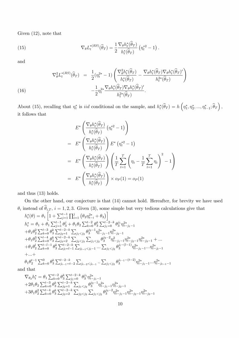
Given (12), note that

(15) r�L�(RS)t (b�T ) = 1

2

r�h�t (b�T )

h�t (b�T )���2t � 1

�:

and

r2�L

�(RS)t (b�T ) =

1

2(�2�t � 1)

r2�h�t (b�T )

h�t (b�T ) � r�h�t (b�T )r�h

�t (b�T )0

h2�t (b�T )!

�12�2�tr�h

�t (b�T )r�h

�t (b�T )0

h2�t (b�T ) :(16)

About (15), recalling that ��t is iid conditional on the sample, and h�t (b�T ) = h���1; ��2; :::; ��t�1;b�T� ;

it follows that

E�

r�h

�t (b�T )

h�t (b�T )���2t � 1

�!

= E�

r�h

�t (b�T )

h�t (b�T )!E����2t � 1

�= E�

r�h

�t (b�T )

h�t (b�T )!0@ 1

T

TXt=1

�t �

1

T

TXt=1

�t

!2� 1

1A= E�

r�h

�t (b�T )

h�t (b�T )!� oP (1) = oP (1)

and thus (13) holds.

On the other hand, our conjecture is that (14) cannot hold. Hereafter, for brevity we have used

�i instead of b�i;T ; i = 1; 2; 3. Given (3), some simple but very tedious calculations give thath�t (�) = �1

h1 +

Pt�1j=1

Qji=1

��2�

2�t�i + �3

�ih�t = �1 + �1

Pt�1j=1 �

j3 + �1�2

Pt�2k=0 �

k3

Pt�2�kj1=0

�j13 �2�t�j1�1

+�1�22

Pt�3k=0 �

k3

Pt�2�kj2=1

Pj1<j2

�j2�13 �2�t�j1�1�2�t�j2�1

+�1�32

Pt�4k=0 �

k3

Pt�2�kj3=2

Pj2<j3

Pj1<j2

�j3�23 �2t�j1�1�2�t�j2�1�

2�t�j3�1 + :::

+�1�l2

Pt�l�1k=0 �k3

Pt�2�kjl=l�1

Pjl�1<jl�1 :::

Pj1<j2

�jl�(l�1)3 �2�t�j1�1:::�

2�t�jl�1

+:::+

�1�t�12

P0k=0 �

k3

Pt�2�kjt�1=t�2

Pjt�2<jt�1

::P

j1<j2�jt�1�(t�2)3 �2�t�j1�1:::�

2�t�jt�1�1

and that

r�2h�t = �1

Pt�2k=0 �

k3

Pt�2�kj1=0

�j13 �2�t�j1�1

+2�1�2Pt�3

k=0 �k3

Pt�2�kj2=1

Pj1<j2

�j2�13 �2�t�j1�1�2�t�j2�1

+3�1�22

Pt�4k=0 �

k3

Pt�2�kj3=2

Pj2<j3

Pj1<j2

�j3�23 �2�t�j1�1�2�t�j2�1�

2�t�j3�1

10

+:::

+l�1�l�12

Pt�l�1k=0 �k3

Pt�2�kjl=l�1

Pjl�1<jl

:::P

j1<j2�jl�(l�1)3 �2�t�j1�1:::�

2�t�jl�1

+:::+

(t� 1) �1�t�22

P0k=0 �

k3

Pt�2�kjt�1=t�2

Pjt�2<jt�1

:::P

j1<j2�jt�1�(t�2)3 �2�t�j1�1::�

2�t�jt�1�1

Without loss of generality, we concentrate on the third term on the RHS of (16). A necessary

condition for (14) is that

E�

1

T

TXt=2

�2�tr�h

�t (b�T )r�h

�t (b�T )0

h2�t (b�T )!

�E 1

T

TXt=2

�2tr�ht(�

y)r�ht(�y)0

ht(�y)

!pr! 0.

Now, given that ��t is iid,

E�

1

T

TXt=2

�2�tr�h

�t (b�T )r�h

�t (b�T )0

h2�t (b�T )!

= E���2�t� 1

T

TXt=2

E�

r�h

�t (b�T )r�h

�t (b�T )0

h2�t (b�T )!!

Given (15) and (16), and the expressions for h�t ; and r�h�t , we can express

3,

r�h�t (b�T )r�h

�t (b�T )0

h2�t (b�T )= gt

�at�1�

�1; at�2�

�2��1; :::; a1�

�2��1:::�

�t�1�= g�t

where a1 > a2 > ::: > at and aT ! 0 as T ! 1: Recall that ��t is equal to �1; �2; :::; �t withprobability 1=T: Let T = 4; and note that we start constructing the term from t = 2; and we

resample ��t from b�t, for t = 1; 2; 3:E�

1

3

4Xt=2

g�t

!=

1

3(E� (g2 (a1�

�1) + g3 (a2�

�1; a1�

�1��2; )) + g4 (a3�

�1; a2�

�1��2; a1�

�1��2��3))

=1

3

1

3

3Xj1=1

g2�a1�j1

�+1

9

3Xj1=1

3Xj2=1

g3�a2�j1 ; a1�j1�j2

�+1

27

3Xj1=1

3Xj2=1

3Xj2=1

g3�a3�j1 ; a2�j1�j2 ; a1�j1�j2�j3

�!

=1

3

�1

3(g2 (a1�1) + g2 (a1�2) + g2 (a1�3))

�+1

3

�1

9

��g3�a2�1; a1�

21

�+ g3 (a2�1; a1�1�2) + g3 (a2�1; a1�1�3) + g3 (a2�2; a1�1�2) + g3

�a2�2; a1�

22

��g3 (a2�2; a1�3�3) + g3 (a2�3; a1�1�3) + g3 (a2�3; a1�3�2) + g3

�a2�3; a1�

23

���3Note that the expansion in term of �s of r�3h�t and r�1h�t follow the same pattern as that for r�2h�t :

11

+1

3

�1

27

�g4�a1�1; a2�

21; a3�

31

�+ g4

�a1�1; a2�

21; a3�

21�2�+ g4

�a1�1; a2�

21; a3�

21�3�

+g4�a1�1; a2�1�2; a3�

21�2�+ g4

�a1�1; a2�1�2; a3�1�

22

�+ g4 (a1�1; a2�1�2; a3�1�2�3)

+g4�a1�1; a2�1�3; a3�

21�3�+ g4 (a1�1; a2�1�3; a3�1�2�3) + g4

�a1�1; a2�3�1; a3�1�

23

�+g4

�a1�2; a2�1�2; a3�

21�2�+ g4

�a1�2; a2�1�2; a3�

21�2�+ g4 (a1�2; a2�1�2; a3�1�2�3)

+g4�a1�2; a2�

22; a3�1�

22

�+ g4

�a1�2; a2�

22; a3�

32

�+ g4

�a1�2; a2�

22; a3�

22�3�

+g4 (a1�2; a2�2�3; a3�1�2�3) + g4�a2�3; a2�2�3; a3�

22�3�+ g4

�a1�2; a2�2�3; a3�2�

23

�+g4

�a1�3; a2�1�3; a3�

21�3�+ g4 (a1�3; a2�1�3; a3�1�2�3) + g4

�a1�3; a2�1�3; a3�1�

23

�+g4 (a1�3; a2�2�3; a3�1�2�3) + g4

�a1�3; a2�2�3; a3�

22�3�+ g4

�a1�3; a2�2�3; a3�2�

23

�+g4

�a1�3; a2�

23; a3�1�

23

�+ g4

�a2�3; a2�

23; a3�2�

23

�+ g4

�a1�3; a2�

23; a3�

33

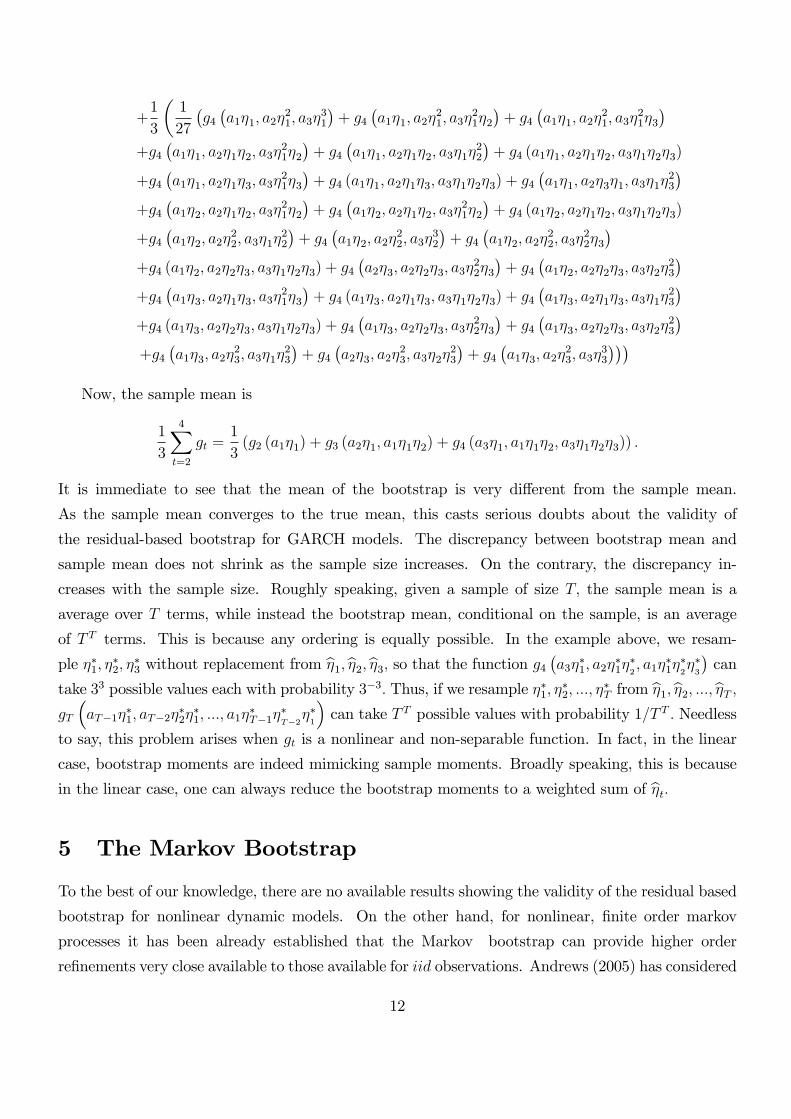
���Now, the sample mean is

1

3

4Xt=2

gt =1

3(g2 (a1�1) + g3 (a2�1; a1�1�2) + g4 (a3�1; a1�1�2; a3�1�2�3)) :

It is immediate to see that the mean of the bootstrap is very di¤erent from the sample mean.

As the sample mean converges to the true mean, this casts serious doubts about the validity of

the residual-based bootstrap for GARCH models. The discrepancy between bootstrap mean and

sample mean does not shrink as the sample size increases. On the contrary, the discrepancy in-

creases with the sample size. Roughly speaking, given a sample of size T; the sample mean is a

average over T terms, while instead the bootstrap mean, conditional on the sample, is an average

of T T terms. This is because any ordering is equally possible. In the example above, we resam-

ple ��1; ��2; �

�3 without replacement from b�1;b�2;b�3; so that the function g4 �a3��1; a2��1��2 ; a1��1��2��3� can

take 33 possible values each with probability 3�3: Thus, if we resample ��1; ��2; :::; �

�T from b�1;b�2; :::;b�T ;

gT

�aT�1�

�1; aT�2�

�2��1; :::; a1�

�T�1�

�T�2��1

�can take T T possible values with probability 1=T T : Needless

to say, this problem arises when gt is a nonlinear and non-separable function. In fact, in the linear

case, bootstrap moments are indeed mimicking sample moments. Broadly speaking, this is because

in the linear case, one can always reduce the bootstrap moments to a weighted sum of b�t:5 The Markov Bootstrap

To the best of our knowledge, there are no available results showing the validity of the residual based

bootstrap for nonlinear dynamic models. On the other hand, for nonlinear, �nite order markov

processes it has been already established that the Markov bootstrap can provide higher order

re�nements very close available to those available for iid observations. Andrews (2005) has considered

12

the case in which the transition density is known in closed form, so that the Markov bootstrap is

indeed a parametric bootstrap, while Horowitz (2003) has considered the case in which the transition

density is unknown. More precisely, Andrews (2005) suggests to recursively resample the data from

the likelihood evaluated at the estimated parameters. Thus, the bootstrap sample is generated by

the same conditional distribution as the original sample, but with the "true" parameters replaced

by the estimated parameters. However, this approach is not directly applicable in our context, as

it is well known that yt; as de�ned in (1) is non markovian, though (yt; �2t ) are jointly markovian.

Nevertheless, if we knew the marginal density of the �; say �� (�) ; then we could draw from it T

iid observations, and use them to recursively construct ht�b�T� and yt in the same manner outlined

in the previous section. In this case, the only di¤erence between the DGP and the bootstrap DGP

is the latter is generated using b�T instead of �y: As a consequence, we could obtain higher orderre�nements along the same lines as in Andrews. Needless to say, this is not particularly useful, as in

general we do not know the marginal density of the errors.

For the case in which the transition density of a Markov process is unknown, Horowitz (2003)

has suggested to draw the observations from a kernel density estimator. For one-dimensional Markov

processes of order q; Horowitz shows that the error in the bootstrap estimate of one-sided (sym-

metrical) probability is OP�T�1=2+�+"

� �OP�T�1+�+"

��; where " > 0 can be set arbitrarily small

and � = s= (2s+ (q + 1)) ; where s � 2; denotes the order of the kernel used in the estimator. Thiscontrasts with the case of known transition density, in which the bootstrap estimate of one-sided

(symmetrical) probability is oP (T�1 log T )�oP�T�3=2 log T

��:

The key point in Horowitz result, stated in his Lemma 14, is that the cumulants of the original and

bootstrap statistics di¤er only of a term of order T�1=2+�+"; which re�ects the uniform rate at which

the estimated conditional density converges to the true one. In fact, because of the markov property,

all moments, as well as smooth functions of them, can be computed via the transition density. Thus

it is enough to control the error between the estimated and the true conditional density, in a uniform

manner.

It is easy to see that ��mixing GARCH processes, with exponentially decaying mixing coe¢ -

cients, are approximate Markov, according to the de�nition of Horowitz (2003, Section 4.3). If we

were interested in making inference on the parameters of the conditional mean of yt; given yt�1; then

we could make independent draws from a kernel density estimator having as conditioning variables

yt�1; :::; yt�q; with q growing at most at a logarithmic rate. We could then regress resulting bootstrap

series, say eyt to estimate the conditional mean parameters, given eyt�1, and proceed in the usualmanner (see e.g. the simulation experiments in Section 5 of Horowitz (2003)).

On the other hand, this approach is not viable, if we are interested in making inference on the

conditional variance parameters. In this case, in fact we have to draw the innovation process from its

13

marginal density estimator. Hereafter, let e�t; t = 1; :::; T be the T iid draws from the kernel density

estimator constructed using b�; where b�t = yt=rht �b�T�; with b�T being the QML estimator de�nedin (2), also let

(17) eht �b�T� = b�1;T "1 + t�1Xj=1

jYi=1

�b�2;Te�2t�i + b�3;T�#;

and �nally let eyt = eht �b�T�e�t; ande��T = argmax

�2�

1

T

TXt=1

eLt(�)= argmax

�2�

�12

TXt=1

lneht(�)� 12

TXt=1

y2teht (�)!

The issue arising in our context, is that the derivatives of the likelihood are a function of the

entire history of the innovations, and so their moments have to be taken with the respect to the joint

density of the �; or because of independence with respect to the product of the marginals. Let eE bethe expectation under the parametric bootstrap law, i.e. the law governing the e�t:Analogously to the case of residual-based bootstrap, in order to ensure the �rst order validity, we

need to ensure that

eE 1T

TXt=2

e�2tr�eht(b�T )r�

eht(b�T )0eh2t (b�T )!

�E 1

T

TXt=2

�2tr�ht(�

y)r�ht(�y)0

ht(�y)

!pr! 0:(18)

Let ep(�i) be the kernel density used to generate the e�; evaluated at �i; and let p (�i) ; be the truedensity of the �: Given (3) and (17), via a Taylor expansion, the left hand side of (18) ; writes as

(19)Z 1

�1:::

Z 1

�1

1

T

TXt=2

�2tr�eht(�y)r�

eht(�y)0eh2t (�y)��ti=1epT (�i)� �ti=1p(�i)� d�1:::d�T ;

plus a term of smaller order.4 Now, via straightforward manipulations, up to a term of smaller order,

�ti=1ep(�i)� �ti=1p(�i)=

tXj=1

�epT (�j)� p(�j)��s 6=jp(�s):4Note that when evaluated at a generic value �; eht(�y) coincide with ht(�y):

14

Thus, even if supx jepT (x)� p(x)j ! 0 as T ! 1; the term in (19) cannot approach zero, as the

estimation errors are summing up. Needless to say, this is due to the fact that ht depends on the

entire history of the innovations.

Therefore, unless we knew the density of the innovations, the Markov bootstrap is not �rst order

valid for the estimation of the conditional variance parameters of a GARCH process.

6 Simulation results

Table 2 in Gonçalves and White (2004, page 209) shows the coverage rates of nominal 95% symmetric

percentile intervals for an ARCH(1) process, both using asymptotic theory and the block bootstrap.

They consider sample sizes T equal to 200 and 500 and, for � = 0 (in their notation, � implies that

�t in (1) follows a iidN (0; 1) distribution). We extend their simulation experiment to the case of

a GARCH(1,1) as in (1), where the true parameter vector is given by��y1; �

y2; �

y3

�0= (0:8; 0:1; 0:8)0 ;

and �t is iidN(0; 1): We use the MBB of Künsch (1989). Since our model is a GARCH(1,1), a more

complicated process than the simulated ARCH(1) of Gonçalves and White (2004, page 209, Table

2), we report results for sample sizes 300 and 500. The number of Monte Carlo replications is set

equal to 500. Table 1 reports the results of coverage rates of nominal 95% symmetric percentile-t

intervals both using the QML asymptotic approximation (ASYM) and our block bootstrap procedure

(Bboot).

For the block bootstrap procedure (Bboot), we have used 500 bootstrap replications. We report

the results for block sizes l = 5; 10; 25 and 50:

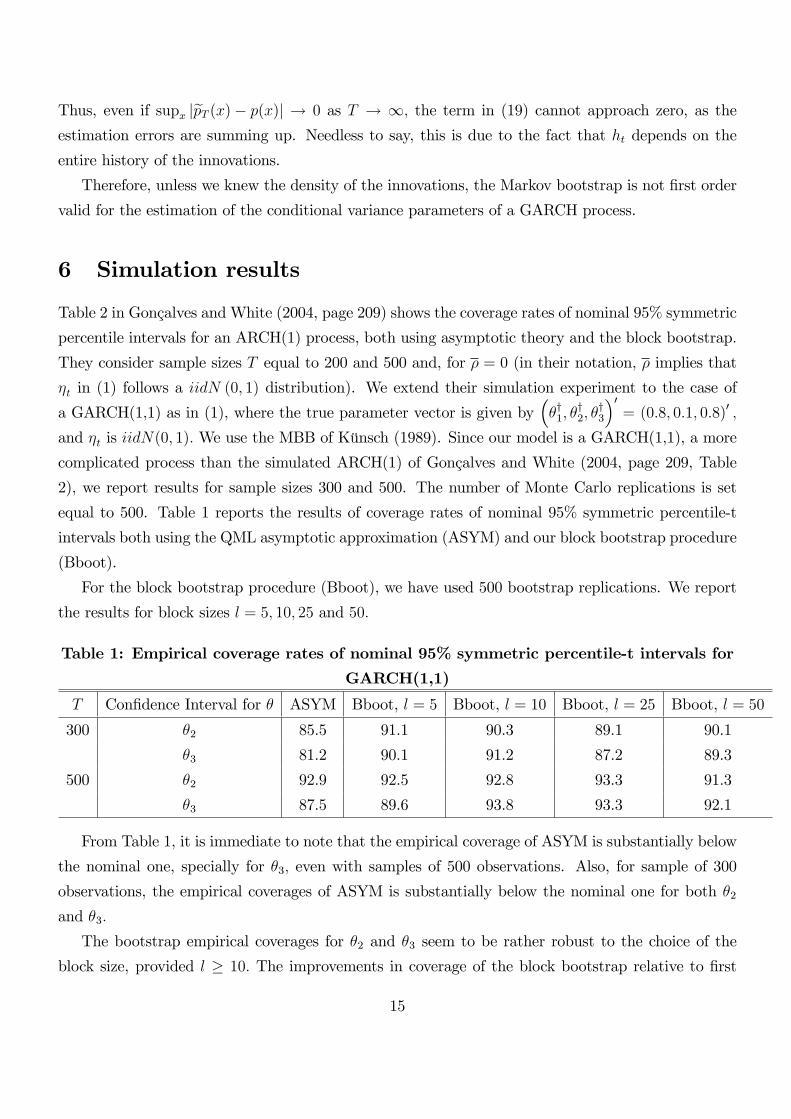
Table 1: Empirical coverage rates of nominal 95% symmetric percentile-t intervals for

GARCH(1,1)

T Con�dence Interval for � ASYM Bboot, l = 5 Bboot, l = 10 Bboot, l = 25 Bboot, l = 50

300 �2 85.5 91.1 90.3 89.1 90.1

�3 81.2 90.1 91.2 87.2 89.3

500 �2 92.9 92.5 92.8 93.3 91.3

�3 87.5 89.6 93.8 93.3 92.1

From Table 1, it is immediate to note that the empirical coverage of ASYM is substantially below

the nominal one, specially for �3; even with samples of 500 observations. Also, for sample of 300

observations, the empirical coverages of ASYM is substantially below the nominal one for both �2and �3:

The bootstrap empirical coverages for �2 and �3 seem to be rather robust to the choice of the

block size, provided l � 10: The improvements in coverage of the block bootstrap relative to �rst

15

order asymptotics are noticeable, specially for �3 for 500 observations, and for both �2 and �3 in

the case of 300 observations. This shows the usefulness of the block bootstrap in this context. The

simulation results of Table 1 rely on iid normal innovations, so that all the moments of �t exist, and

thus the necessary condition in Theorem 1 and the su¢ cient conditions in Theorem 2 are satis�ed.

16

7 Appendix

Proof of Theorem 1: As we are interested in necessary conditions it su¢ ces to consider T 1=2�b�i;T � �yi� :

We �rst need to establish the existence of a stochastic expansion of T 1=2�b�i;T � �yi� up to a term

of order o�T�

k�12

�: Given A1, and assuming that E(�4t ) < 1; it follows that T 1=2

�b�i;T � �yi� isasymptotically normal (see e.g. Bollerslev and Wooldridge 1992), thus

T 1=2�b�T � �y� = T 1=2�T = OP (1):

Let LT (�) = 1T

PTt=1 Lt (�) ; then the Taylor expansion of r�LT

�b�T� around �y; up to the k orderwrites as

0 = r�LT��y�+r2

�LT��y��T

+1

2

0BB@P3

j1=1

P3j2=1

r�1�j1�j2LT��y��T;j1�T;j2P3

j1=1

P3j2=1

r�2�j1�j2LT��y��T;j1�T;j2P3

j1=1

P3j2=1

r�3�j1�j2LT��y��T;j1�T;j2

1CCA

+:::+1

k!

0BB@P3

j1=1:::P3

jk=1r�1�j1 :::�jk

LT��y��T;j1 � �T;j2 � :::� �T;jkP3

j1=1:::P3

jk=1r�2�j1 :::�jk

LT��y��T;j1 � �T;j2 � :::� �T;jkP3

j1=1:::P3

jk=1r�1�j1 :::�jk

LT��y��T;j1 � �T;j2 � :::� �T;jk

1CCA+ek+1;T ;

where r�1�j1 :::�jkLT��y�denote the k + 1�th derivative with respect to �1; �j1 ; :::; �jk ; and �T;jk the

jk�th component of �T : Thus,

T 1=2�b�T � �y�

=��r2

�LT��y���1 �

T 1=2r�LT��y�

+1

2T 1=2

0BB@P3

j1=1

P3j2=1

r�1�j1�j2LT��y��T;j1�T;j2P3

j1=1

P3j2=1

r�2�j1�j2LT��y��T;j1�T;j2P3

j1=1

P3j2=1

r�3�j1�j2LT��y��T;j1�T;j2

1CCA+ :::

+1

k!T 1=2

0BB@P3

j1=1:::P3

jk=1r�1�j1 :::�jk

LT��y��T;j1 � �T;j2 � :::� �T;jkP3

j1=1:::P3

jk=1r�2�j1 :::�jk

LT��y��T;j1 � �T;j2 � :::� �T;jkP3

j1=1:::P3

jk=1r�1�j1 :::�jk

LT��y��T;j1 � �T;j2 � :::� �T;jk

1CCA1CCA

+T 1=2ek+1;T :

Hereafter, rk�LT

��y�is the matrix with generic element r�j1 :::�jk

LT��y�; ji = 1; 2; 3 for all i: A few

calculations give,

17

r�Lt��y�=1

2

r�ht��y�

ht��y� �

�2t � 1�

r2�Lt��y�=

1

2

��2t � 1

� r2�ht��y�

ht��y� �

r�ht��y�r�ht

��y��

h2t��y� !

�12�2tr�ht

��y�r�ht

��y��

h2t��y�

r3�Lt��y�

=1

2

��2t � 1

� r3�ht��y�

ht��y� �

r�ht��y��r2

�ht��y��

h2t��y� +

2�r�ht

��y��r�ht

��y�r�ht

��y���

h3t��y� !

+1

2�2t

�r�ht

��y��r�ht

��y�r�ht

��y���

h3t��y� �

r�ht��y��r2

�ht��y��

h2t��y� !

It now becomes apparent, that in the computation of r3�lt��y�; by the law of iterated expectations

E

"�2t

�r�ht

��y��r�ht

��y�r�ht

��y���

h3t��y� !#

= E

"�r�ht

��y��r�ht

��y�r�ht

��y���

h3t��y� #

and the term of higher order for generic k is

E

�r�ht

��y��r�ht

��y� ::r�ht

��y���

hkt��y� !

where at the numerator we have k kronecker products of �rst derivatives.

From Lemma 1 in Lumsdaine (1996, equations A1.1-A1.4), it follows that for i = 1; 2; 3

E

�r�iht(�

y)ht(�y)

�k!is of the same order of magnitude as E

�y2kt�j

hkt (�y)

�= E

�hkt�j(�y)hkt (�y)

�2kt�j

�for any

j < t: Therefore, a necessary condition for E�r�1�j1 :::�jk

LT��y��<1 is that E

��2kt�j

�<1:

Indeed, this is also a su¢ cient condition. In fact, Ling and McAleer (2003, p.304) show that

a su¢ cient condition for the existence of E�(r�ht(�y)�r�ht(�y))

h2t(�y)

�is that E(�4i ) < 1: The same

argument can be used to show a su¢ cient condition for E�r�1�j1 :::�jk

LT��y��<1 is that E

��2kt�<

1:

18

Now, in order to have an Edgeworth expansion for the LHS of (11) ; up to the k�th term, weneed the existence of the (k+2) moment of the (k+2) derivative of the score and the outerproduct,

which in turn requires that E��2(k+2)(k+4)t

�<1:

�Hereafter, let P � denoting the probability law governing the block bootstrap, E� and V ar� the

mean and variance operator under P �; alsopr�! and d�! denote convergence in probability and in

distribution under P �; conditionally on the sample.

Proof of Theorem 2: As for �rst order validity, provided E (�8t ) < 1; then t�i;Td! N(0; 1), by

Bollerslev and Wooldridge (1992).

We now outline the �rst order validity of the block bootstrap based on the resampling of the

log-likelihood. By a mean value, expansion

pT�b��T � b�T� =

� 1T

TXt=1

r2�L

�t (�

�T )

!�11pT

TXt=1

r�L�t (b�T );

where ��T 2

�b��T ;b�T� and r�L�t (b�T ) = r�L

�t (b�T ) � E� �r�L

�t (b�T )� : It is immediate to see that

E��

1pT

PTt=1r�L

�t (b�T )� = 0 and V ar�

�1pT

PTt=1r�L

�t (b�T )� = eA�T ; with the RHS de�ned in (8).

Recalling that the bootstrap sample consists of b independent blocks, by Theorem 3.5 in Kün-

sch (1989), eA��1=2T1pT

PTt=1r�L

�t (b�T ) d�! N(0; I3): Also, as b��T � b�T pr�! 0; it immediately follows

that� bB��1T

eA�T bB��1T

��1=2pT�b��T � b�T� d�! N(0; I3); and thus

pT�b��i;T � b�i;T� =e��T;ii d�! N(0; 1);

where e��T;ii is the ii�th element of eA�1=2T : Let b��T;ii = � bB��1TbA�T bB��1T

�1=2ii; and note that t��i;T =�p

T�b��i;T � b�i;T� =e��T;ii� b�T;iib��T;ii ; where b�T;ii is de�ned just below equation (8). Therefore, we need to

show that, b�T;iib��T;ii pr�! 1; conditional on the sample. Recalling (4), and (6), it is immediate to see that

E�� bA�T� = bAT +OP � l

T

�;

and thus� bA�T � bAT� pr�! 0: The �rst order validity then follows.

As for higher order re�nements, we proceed by showing that the moments conditions imposed

on the innovation term ensure that the statement in Lemma 13, 14 and 15 in Andrews (2002) apply

also in our context.

De�ne the bootstrap analog of (10), that is:

(20) f �i;t;d1;k (�) =�r�iL

�t (�) ; :::;r

d1;k�i

�r�L

�t (�)

�;r�iL

�tr�iL

�t (�)

0 ; :::;rd1;k��i

�r�L

�tr�L

�t (�)

0��;

19

where r�iL�t (�) = r�iL

�t (�)� E� (r�iL

�t (�)) ; and

r�iL�tr�iL

�t (�)

0 = r�iL�tr�iL

�t (�)

0 � E��r�iL

�tr�iL

�t (�)

0� : Also, de�neST;i;d1;k(�

y) =1

T

TXt=1

fi;t;d1;k(�y)

S�T;i;d1;k(b�T ) = 1

T

TXt=1

f �i;t;d1;k(b�T )

Given A1, d1 � k+2; > 0; by Lemma 13 in Andrews (2002), there exists an in�nite di¤erentiablefunction G(�); with G(Si) = 0 and G(S�i ) = 0; where Si = E

�ST;i;d1;k

��y��, S�i = E

��S�T;i;d1;k

�b�T�� ;such that, for k = 2; 3

(21) limT!1

supzT k=2

��Pr (t�i;T � z)� Pr �T 1=2G �ST;i;d1;k ��y�� � z��� = 0and

(22) limT!1

supzT k=2

���Pr �et�i;T � z�� Pr�T 1=2G�S�T;i;d1;k(b�T )� � z���� = 0Leti;k;T = T 1=2

�Si;T;d1;k(�

y)� E�Si;T;d1;k(�

y)��and�i;k;T = T

1=2�S�i;T;d1;k(

b�T )� E� �S�i;T;d1;k(b�T )�� ;and let i;k;T;j be the j � th element of i;k;T : De�ne

(23) vi;T;k = E�T�(m)�m�=1i;k;T;j�

�and let vi;k = limT!1 vi;T;k; and

(24) evi;T;k = E� �T�(m)�m�=1�i;k;T;j��where �(m) = 1=2 if m is odd and 0 if m even, and 2 � m � k + 2: Along the lines of the proof ofLemma 14, in Andrews (2002),we need to show that

(25) limT!1

T k=2P���T 1=2E� ��m�=1�i;k;T;��� T 1=2E ��m�=1i;k;T;���� > cT��� = 0

for some c > 0; and

(26) limT!1

T ����T 1=2E ��m�=1i;T;j��� lim

T!1T 1=2E

��m�=1i;T;j�

���� = 0Hereafter, as the arguments used in the proof are the same across all i; when there is no risk on

confusion, we omit the subscript i: Let fi;t;d1;k��y�and f �i;t;d1;k

�b�T� be de�ned as (10) and (20),respectively. De�ne f t;k = fi;t;d1;k

��y��E

�fi;t;d1;k

��y��and f

�t;k = f

�i;t;d1;k

�b�T��E� �f �i;t;d1;k �b�T��;20

also let Yj =P

t2bj f t;k;eYj =Pt2bj f

�t;k; and Y

�j =

Pt2b�j

f�t;k, where for j = 1; :::; Tl; Tl = T � l + 1;

bj = (j; :::; j + l � 1) j = 1; :::; b and b�j is an iid discrete uniform random variable which is equal to

bj with equal probability 1=Tl: As shown in Andrews (2002), the most di¢ cult case is that of m = 3:

Now,

T 1=2E���3�=1

�i;T;�

�= T�1

bXj1=1

bXj2=1

bXj3=1

E��Y �j1Y

�j2Y �j3�

= T�1bE��Y �31�= T�1bT�1l

TlXj=1

eY 3j :If for some C <1; and for i; j = 1; 2; 3 E

��rd1;k+d2;k�

�r�iLT (�)r�iLT (�)

0��3p� < C uniformlyin a neighborhood of �y; with d1;k � k + 3; d2;k � k + 1; p de�ned as below and if � + < 1=2; thenfrom Andrews (2001),

(27) limT!1

T k=2P

T�1bT�1l

TlXj=1

���eY mj � Y mj��� > T��! = 0:

Given (27), in order to show (25), one has to show that B1 and B2 below approach zero, where

B1 = limT!1

T k=2P

�����T�1bT�1lTlXj=1

�Y 3j � E

�Y 3j������� > T �

!

and that

B2 = limT!1

T ���T�1bE �Y 31 �� T 1=2E ��3�=1i;T;���� :

By Markov inequality and a double application of Yokoyama-Doukan inequality (Doukhan 1995,

p.25-30), there exists a constant C and � > 0 such that,

B1 � CT k=2+p(��1)E

�����bT�1lTlXj=1

�Y 3j � E

�Y 3j�������

p

� C limT!1

T k=2+p(��1)bp=2l3p=2�E��f 1;k��3p+4�� 3p(3+�)

(3+�)(3(p+�)+�)

� C limT!1

T k=2+p(��1)T p=2T p �E��f 1;k��3p+4�� 3p(3+�)

(3+�)(3(p+�)+�)(28)

Thus, B1 ! 0; provided p > k2(1=2� ��) and if E

��f 1;k��3p+4� <1:Also, by the proof of Lemma 14 in Andrews (2001), it follows that for the case of m = 5; we need

p > k=(3� 2� � 4 ); requiring � + 2 < 3=2; which is implied by � + < 1=2 and E��f 1;k��5p+4� <1:

Given (10) and the last line of (28), it su¢ ce that the �rstmp+4�-th moments of all score derivatives

up to order (d1;k + d2;k) exist: In the proof of Theorem 1 we have shown that E��rr1�iLT��y��r2�

<

21

1 if and only if E��2(r1+r2)t�j

�< 1; by the same argument, and as a straightforward conse-

quence of the chain rule E��rr1�i

�LT��y�LT��y�0��r2�

< 1 if and only if E��2(r1+r2+1)t�j

�< 1:

Now, recalling that 2 � m � k + 2; setting � = 1=4; it follows that E���f 1;k��mp+4�� < 1 and

E��rd1;k+d2;k�

�r�ilt (�)r�ilt (�)

0��mp� < 1 if E��2(d1;k+d2;k+2)(k+2)pt

�< 1; where d1;k � k + 3;

d2;k � k + 1; and p > k=22(1=2��� ) : Thus, the left hand side of (28) is approaching zero, provided

E��2(2k+6)(k+2)pt

�<1:

As for B2; along the lines of proof of Lemma 14 in Andrews (2002), recalling that l = T ;

T�1bE�Y 31�� T 1=2E

��3�=1i;T;�

�=

1

lE

lXi=1

f i;k

!3� 1

T

TXi1=1

TXi2=1

TXi2=1

f i1;kf i2;kf i3;k

=l�1X

i1=�l+1

l�1Xi2=�l+1

�1� (i1 + i2)

l

�E�f 0;kf i1;kf i2;k

��

T�1Xi1=�T+1

T�1Xi2=�T+1

�1� (i1 + i2)

T

�E�f 0;kf i1;kf i2;k

�:

Now,

T �

�����l�1X

i1=�l+1

l�1Xi2=�l+1

E�f 0;kf i1;kf i2;k

��

T�1Xi1=�T+1

T�1Xi2=�T+1

E�f 0;kf i1;kf i2;k

������! 0

by the Doukhan mixing inequality (1995, p.9), provided > �: Also,

T ��1

�����T�1X

i1=�T+1

T�1Xi2=�T+1

(i1 + i2)E�f 0;kf i1;kf i2;k

������! 0

by mixing inequality, and

T ��

�����l�1X

i1=�l+1

l�1Xi2=�l+1

(i1 + i2)E�f 0;kf i1;kf i2;k

������! 0;

provided � < : The statement in (25) follows by the same argument used to show that B2 ! 0:

Finally, from (25) and (26) it follows that

limT!1

T k=2P�jevi;T;k � vi;kj > T �� = 0:

Now, de�ne v�i;T;k = evi;T;k � � �i : In our context, the score is a martingale di¤erence sequence, andso there is no need to take into account the cross terms in the computation of the covariance of t�i;T :

Thus, from part (ii) in Lemma 15 in Andrews (2002), setting � = 0 in his notation, it follows that

(29) limT!1

T k=2P���ev�i;T;k � vi;k�� > T �� = 0:

22

Given (21) and (22), in order to establish the existence of an Edgeworth expansion up to order k; it

su¢ ces to show that

(30) limT!1

T k=2 supz2R

�����Pr �T 1=2G �ST;i;d1;k ��y�� � z�� 1 +

kXi=1

T�1=2�i (@=@z; vi;k)

!�(z)

����� = 0and

(31) limT!1

T k=2 supz2R

�����Pr�T 1=2G�S�T;i;d1;k �b�T�� � z�� 1 +

kXi=1

T�1=2�i�@=@z; v�i;k

�!�(z)

����� = 0:Along the lines of Lemma 16 in Andrews (2002), and given Assumption A2 and

E

��2(d1;k+d2;k+2)(k+2)pt

�< 1; (30) follows from Theorem 3.1 Bhattacharya (1987) and Götze and

Hipp (1983), while (31) follows from Theorem 3.3 Bhattacharya (1987) and Chandra and Gosh

(1979).

Now, recalling (21) and (22), as well as (29), setting k = 2; 3 respectively, it follows that

limT!1

T P

�supx2R

��P � �t��i;T � x�� P (t�i;T � x)�� > T�(1=2+�)� = 0and

limT!1

T 3=2 P

�supx2R

��P � ���t��i;T �� < x�� P (jt�i;T j � x)�� > T�(1+�)� = 0:It remains to show that the bootstrap error in the rejection probability are indeed of the same

order of the error in the bootstrap estimate of one-sided and symmetrical probability. This follows

by the same argument used in the proof of Theorem 2 in Andrews (2002).

23

8 References

Andrews, D. W. K. (2001), Higher-Order Improvements of a Computationally Attractive k�StepBootstrap for Extremum Estimators, Cowles Foundation Discussion Paper #1230R.

Andrews, D. W. K. (2002), Higher-Order Improvements of a Computationally Attractive k�StepBootstrap for Extremum Estimators, Econometrica 70, 119-162.

Andrews, D. W. K. (2005), High Order Improvements of the Parametric Bootstrap for Markov

Processes, in Identi�cation and Inference in Econometric Models: A Festschrift in Honor of

Thomas J. Rothemberg, ed. by D.W.K. Andrews and J.H. Stock, Cambridge University Press.

Bhattacharya R. N. (1987), Some Aspects of Edgeworth Expansions in Statistics and Probability,

in New Perspectives in Theoretical and Applied Statistics, ed. by M.L. Puri, J.P. Vilaploma,

and W. Wertz, Wiley.

Bollerslev, T. (1986), Generalized Autoregressive Conditional Heteroskedasticity. Journal of Econo-

metrics 31, 307-327.

Bollerslev, T., and J. M. Wooldridge (1992), Quasi-Maximum Likelihood Estimation and Inference

in Dynamic Models with Time-varying Covariances, Econometric Reviews 11, 143-172.

Bose, A. (1988), Edgeworth Correction by Bootstrap in Autoregressions, Annals of Statistics 16, 4,

1709-1722.

Carrasco, M., and X. Chen (2002), Mixing and Moment Properties of Various GARCH and Sto-

chastic Volatility Models, Econometric Theory 18, 17-39.

Chandra, T.K., and J.K. Ghosh (1979), Valid Asymptotic Expansions for the Likelihood Ratio

Statistic and Other Perturbed Chi-Square Variables, Sankhya, 41, Series A, 22-47.

Christo¤ersen, P. and S. Gonçalves (2005), Estimation Risk in Financial Risk Management, Journal

of Risk 7, 1-29.

Doukhan, P. (1995), Mixing Properties and Examples, Springer and Verlag, New York.

Gonçalves, S. and L. Kilian (2004), Bootstrapping Autoregressions with Conditional Heteroskedas-

ticity of Unknown Form, Journal of Econometrics 123, 89-120.

Gonçalves, S. and L. Kilian (2007), Asymptotic and Bootstrap Inference for AR(1) Processes withConditional Heteroskedasticity, Econometric Reviews forthcoming.

24

Gonçalves, S. and H. White (2004), Maximum Likelihood and the Bootstrap for Nonlinear Dynamic

Models, Journal of Econometrics 119, 199-219.

Götze, F. and C. Hipp (1983), Asymptotic Expansions for Sums of Weakly Dependent Random

Vectors. Zeitschrift für Wahrscheinlickheits Theorie und Verwandte Gebiete 64, 211-239.

Götze, F. and C. Hipp (1994), Asymptotic Distributions of Statistics in Time Series, Annals of

Statistics 22, 2062-2088.

Hall, P. (1992), The Bootstrap and Edgeworth Expansion. New York: Springer.

Hall, P., and J. L. Horowitz (1996), Bootstrap Critical Values for Tests based on Generalized-

Method-of-Moments Estimators, Econometrica 64, 4, 891-916.

Hidalgo, F.J., and P. Za¤aroni (2007), A Goodness of Fit Test for ARCH(1 ), Journal of Econo-

metrics, forthcoming.

Horowitz, J.L. (2003) Bootstrap Methods for Markov Processes, Econometrica, 71, 1049-1082.

Inoue A., and L. Kilian (2002), Bootstrapping Autoregressive Processes with Possible Unit Roots,

Econometrica 70, 1, 377-393.

Kreiss, J.-P., and J. Franke (1992), Bootstrapping Stationary Autoregressive Moving-Average Mod-

els, Journal of Time Series Analysis 13, 4, 297-317.

Künsch, H. R. (1989), The Jackknife and the Bootstrap for General Stationary Observations, Annals

of Statistics 17, 1217-1241.

Ling, S.Q., and M. McAleer, (2003), Asymptotic theory for a vector ARMA-GARCH model, Econo-

metric Theory 19, 280-310.

Linton, O. (1997), An Asymptotic Expansion in the GARCH(1,1) Model. Econometric Theory 13,

558-581.

Lumsdaine, R. L. (1996), Asymptotic Properties of the Maximum Likelihood Estimator in GARCH(1,1)

and IGARCH(1,1) Models. Econometrica 64, 3, 575-596.

Mancini, L., and F. Trojani, (2005), Robust Semiparametric Bootstrap Methods for Value at Risk

Prediction under GARCH-type Volatility Processes, SSRN Working Paper, University of St.

Gallen.

25

Pascual L., J. Romo and E. Ruiz (2006), Bootstrap Prediction for Returns and Volatilities in

GARCH Models, Computational Statistics and Data Analysis 50, 2293-2312.

26