1

Boosted Bayesian Network ClassifiersYushi Jing Vladimir Pavlovic James M. Rehg

College of Computing Department of Computer Science College of ComputingGeorgia Institute of Technology Rutgers University Georgia Institute of Technology

Atlanta, GA, 30332 Piscataway, NJ, 08854 Atlanta, GA, 30332

Abstract— The use of Bayesian networks for classificationproblems has received significant recent attention. Although com-putationally efficient, the standard maximum likelihood learningmethod tends to be suboptimal due to the mismatch betweenits optimization criteria (data likelihood) and the actual goal ofclassification (label prediction accuracy). Recent approaches tooptimizing classification performance during parameter or struc-ture learning show promise, but lack the favorable computationalproperties of maximum likelihood learning. In this paper wepresent Boosted Bayesian Network Classifiers, a framework tocombine discriminative data-weighting with generative trainingof intermediate models. We show that Boosted Bayesian networkClassifiers encompass the basic generative models in isolation,but improve their classification performance when the modelstructure is suboptimal. This framework can be easily extendedto temporal Bayesian network models including HMM andDBN. On a large suite of benchmark data-sets, this approachoutperforms generative graphical models such as naive Bayes,TAN, unrestricted Bayesian network and DBN in classificationaccuracy. Boosted Bayesian network classifiers have comparableor better performance in comparison to other discriminativelytrained graphical models including ELR-NB, ELR-TAN, BNC-2P,BNC-MDL and CRF. Furthermore, boosted Bayesian networksrequire significantly less training time than all of the competingmethods.

I. I NTRODUCTION

A Bayesian network is an annotated directed graph thatencodes the probabilistic relationships among variables ofinterest [42]. The explicit representation of probabilistic rela-tions can exploit the structure of the problem domain, makingit easier to incorporate domain knowledge into the modeldesign. In addition, the Bayesian network has a modularand intuitive graphical representation which is very beneficialin decomposing a large and complex problem representationinto several smaller, self-contained models for tractabilityand efficiency. Furthermore, the probabilistic representationcombines naturally with the EM algorithm to address problemswith missing data. These advantages of Bayesian networksand generative models as a whole, make them an attractivemodelling choice.

In many problem domains where a Bayesian network isapplicable and desirable, we may want to infer the label(s)for a subset of the variables (class variables) given an in-stantiation of the rest (attributes). Bayesian network clas-sifiers [18] model the conditional distribution of the classvariables given the attributes and predict the class with thehighest conditional probability. Bayesian network classifiershave been applied successfully in many application areas

including computational molecular biology [49] [38] [28],computer vision [51] [44] [48], relational databases [19], textprocessing [11] [35] [31], audio processing [43] and sensorfusion [40]. Its simplest form, the naive Bayes classifier, hasreceived significant amount of attention [33] [15] [37].

However, standard Maximum Likelihood (ML) parameterlearning in Bayesian network classifiers tends to be subop-timal [18]. It optimizes the joint likelihood, rather than theconditional likelihood, a score more closely related to theclassification task. Unlike the joint likelihood, however, theconditional likelihood cannot be expressed in a log linear form,therefore no closed form solution is available for the optimalparameters. Recently there has been substantial interest indiscriminative training of generative models coupled withadvances in discriminative optimization methods for complexgraphical models [23] [35] [31] [6] [2] [50].

Under the correct model structure, the parameters thatmaximize the likelihood also maximize the conditional like-lihood (see section III). For this reason, structure learn-ing [10] [25] [20] [7] [26] [32] can potentially be usedto improve the classification accuracy. However, experimentsshow that learning an unrestricted Bayesian network fails tooutperform naive Bayes in classification accuracy on a largesample of benchmark data [18] [24]. Friedman et al. attributethis to the mismatch between the structure selection criteria(data likelihood) and the actual goal for classification (labelprediction accuracy). They proposed Tree Augmented NaiveBayes (TAN) [18], a structure learning algorithm that learnsa maximum spanning tree from the attributes, but retainsnaive Bayes model as part of its structure to bias towardsthe estimation of conditional distribution. BNC-2P [24], onthe other hand, is a heuristic structure learning method witha discriminative scoring function. Since BNC-2P relaxes thetree structure assumption of TAN and directly maximizesthe conditional likelihood, it is shown to outperform naiveBayes, TAN, and generatively trained unrestricted networks.Although the structures in TAN and BNC-2P are selecteddiscriminatively, the parameters are trained via ML trainingfor computational efficiency.

In this work we propose a new framework for discriminativetraining of Bayesian networks. Similar to a standard boostingapproach, we recursively form an ensemble of classifiers.However in contrast to situations where the weak classifiersare trained discriminatively, the “weak classifiers” in ourmethods are trained generatively to maximize the likelihoodof weighted data. Our approach has two benefits. First, ML

2

training of generative models is dramatically more efficientcomputationally than discriminative training. By combiningmaximum likelihood training with discriminative weightingof data, we obtain a computationally efficient method fordiscriminatively training a general Bayesian network. Second,our classifiers are constructed from generative models. This isimportant in many practical problems where generative modelsare desired or appropriate.

This work builds on our earlier effort to combine boostingwith Dynamic Bayesian network in the application of audio-visual speaker detection [8] [39]. Preliminary results on theBAN algorithm were published in [27].

The paper makes three contributions:1) We introduce a new discriminative structure learning

method, called Boosted Augmented Naive Bayes (BAN)classifier. We demonstrate that BAN is easy to imple-ment and computationally efficient, with classificationaccuracy superior to naive Bayes, TAN, BNC-2P, BNC-MDL, HGC and comparable to ELR.

2) We interpret a Boosted Bayesian network classifier asa graphical model consisting of a collection of En-semble Bayesian Network models, and present the firstcomprehensive empirical evaluation and comparison ofBoosted Naive Bayes against competing methods on alarge number of standard datasets.

3) We extend Boosted Bayesian network framework toinclude temporal models such as Dynamic BayesianNetworks (DBNs) and empirically demonstrate thatBoosted-DBN outperforms regular DBN in the tasks ofsensor fusion and label sequence predictions. Further-more, we demonstrate that Boosted-DBN has classifi-cation accuracy comparable with Conditional RandomFields (CRFs) [31], at the same time, have less compu-tational cost in training.

This paper is divided into 11 sections. Section 1 through 3review the formal notations of Bayesian networks and parame-ter learning methodologies. Section 4 introduces AdaBoost asan effective way to improve the classification accuracy of naiveBayes. Section 5 and 6 extend this work to structure learningand proposes the BAN structure learning algorithm. Section 7extends this work to temporal models by proposing BoostedDynamic Bayesian Network Classifiers. Section 8 contains theexperiments and analysis for BAN structure learning algorithmand Boosted Dynamic Bayesian Network Classifiers. Thelast three sections contain related works, conclusions andacknowledgements.

II. BAYESIAN NETWORK CLASSIFIER

A Bayesian networkB is a directed acyclic graph thatencodes a joint probability distribution over a set of randomvariablesX = {X1, X2, . . . , XN} [42]. It is defined by thepair B = {G, θ}. G is the structure of the Bayesian network.θ is the vector of parameters that quantifies the probabilisticmodel.B represents a joint distributionPB(X), factored overthe structure of the network where

PB(X) =N∏

i=1

PB(Xi|Pa(Xi)) =N∏

i=1

θXi|Pa(Xi).

We setθxi|Pa(xi) equal toPB(xi|Pa(xi)) for each possiblevalue ofXi andPa(Xi)1. For notational simplicity, we definea one-to-one relationship between the parameterθ and theentries in the local Conditional Probability Table. Given aset of i.i.d. training dataD = {x1, x2, x3, . . . , xM}, the goalof learning a Bayesian networkB is to find a {G, θ} thataccurately models the distribution of the data. The selectionof θ is known as parameter learning and the selection ofG isknown as structure learning.

The goal of a Bayesian network classifier is to correctlypredict the label for classXc ∈ X given a vector of attributesXa = X\Xc. A Bayesian network classifier models thejoint distribution P (Xc, Xa) and converts it to conditionaldistribution P (Xc|Xa). Prediction forXc can be obtainedby applying an estimator such as MAP to the conditionaldistribution.

III. PARAMETER LEARNING

The Maximum Likelihood (ML) method is one of the mostcommonly used parameter learning techniques. It choosesthe parameter values that maximize the Log Likelihood (LL)score, a measure of how well the model represents the data.Given a set of training dataD with M samples and aBayesian Network structureG with N nodes, the LL scoreis decomposed as:

LLG(θ|D) =M∑i=1

logPθ(Di) =M∑i=1

N∑j=1

log θx ij |Pa(xj)

i(1)

= M∑x∈X

P a(x)∈P a(X)

PD(x|Pa(x)) log θx|Pa(x).

LLG(θ|D) is maximized by simply setting each parameterθx|Pa(x) to PD(x|Pa(x)), the empirical distribution of the dataD. For this reason, ML parameter learning is computationallyefficient and very fast in practice.

However, the goal of a classifier is to accurately predict thelabel given the attributes, a function that is directly tied to theestimation of the conditional likelihood. Instead of maximizingthe LL score, we would prefer to maximize the ConditionalLog Likelihood (CLL) score. As pointed out in [18], the LLscore factors as

LLG(θ|D) = CLLG(θ|D) +M∑i=1

logPθ(x ia ),

where

CLLG(θ|D) =M∑i=1

logPθ(x ic |x i

a ) (2)

= M∑

xa∈Xaxc∈Xc

PD(xcxa) logPθ(xc|xa). (3)

1We use capital letters to represent random variable(s) and lowercase lettersto represent their corresponding instantiations. Subscripts are used as variableindices and superscripts are used to index the training data.Pa(Xi) representsthe parent node ofXi and Paj(Xi) is the jth instantiation ofPa(Xi) inthe training data. In this paper, we assume all of the variables are discreteand fully observed in the training data.

3

TABLE I

BOOSTEDPARAMETER LEARNING ALGORITHM.

1) Given a base structureG and the training dataD, whereM is the number of training cases.D = {x 1c x 1

a , x 2c x 2

a , . . . , x Mc x M

a } andxc ∈ {−1, 1}.2) Initialize training data weights withwi = 1/M, i = 1, 2, . . . , M3) Repeat fork = 1, 2, . . .

• Given G,θk is learned through ML parameter learning on the weighted dataDk.• Compute the weighted error,errk = Ew[1xc 6=fθk

(xa)], βk = 0.5 log 1−errkerrk

• Update weightswi = wi exp{−βkx ic f θk (x i

a )} and normalize.4) Ensemble output: sign

∑k βkf θk (xa)

Given the correct network structure G, parameters that max-imizes LLG also maximizes CLLG. However, in practice thestructure may be incorrect and ML learning will not optimizethe CLL score, which can result in a suboptimal classificationdecision. Equation 3 is maximized when

Pθ(xc|xa) =θxc

∏θxa|Pa(xa)∑

xc

θxc

∏θxa|Pa(xa)

= PD(xc|xa). (4)

However, for a generative model such as a Bayesian network,Equation 4 cannot be expressed in log-linear form and has noclosed form solution. A direct optimization approach requirescomputationally expensive numerical techniques. For example,the ELR method of [23] uses gradient descent and line searchto directly maximize the CLL score. However, this approach isunattractive in the presence of a large feature space, especiallywhen used in conjunction with structure learning.

IV. B OOSTEDPARAMETER LEARNING

A. Ensemble Model

Instead of maximizing the CLL score for a single Bayesiannetwork model, we are going to take the ensemble approachand maximize the classification performance of the ensembleBayesian network classifier.

Given the classxc and the attributesxa, an ensemble modelhas the general form:

Fxc(xa) =K∑

k=1

βkfk,xc(xa). (5)

wherefk,xc(xa) is the classifier confidence on selecting label

xc given xa, andβk is its corresponding weight. In the casewhere xc ∈ {−1, 1}, fk,xc(xa) is typically defined as thefollowing:

fk,xc(xa) = xcfk(xa) (6)

wherefk(xa) is the output of each classifier givenxa. Equa-tion 5 can be expressed as a conditional probability distributionoverXc given the additive model F:

PF (xc|xa) =exp{Fxc

(xa)}∑x′c∈Xc

exp{Fx′c (xa)}. (7)

In binary classification, Equation 7 is then updated as:

PF (xc|xa) =exp{xcF (xa)}

exp{F (xa)} + exp{−F (xa)}

=exp{xcF (xa)}

exp{xcF (xa)} + exp{−xcF (xa)}

=1

1 + exp{−2xcF (xa)}. (8)

Similar to Equation 3, the negative CLL score for the ensembleBayesian network classifier can be defined as:

−CLLF (F |D) =M∑i=1

log1

PF (x ic |x i

a )(9)

= M∑

xa∈Xaxc∈Xc

PD(xcxa) log1

PF (xc|xa).(10)

B. Exponential Loss Function as an upper bound on thenegative CLL score

As an alternative to the CLL score, we are proposing tominimize the classification error for binary ensemble classifiervia the following loss function.

LossF =M∑i=1

Θ(−x ic F (x i

a )),Θ(z) ={

0 for z < 01 otherwise

LossF is simply the number of incorrectly predicted classlabels in the training data. An upper bound on Equation 11 isgiven by the following exponential loss function [17]:

ELFF =M∑i=1

exp{−x ic F (x i

a )} (11)

Solving forxcF (xa) in Equation 8 and combining with Equa-tion 11, we have

ELFF =M∑i=1

exp{

12

log1 − PF (x i

c |x ia )

PF (x ic |x i

a )

}(12)

=M∑i=1

√1 − PF (x i

c |x ia )

PF (x ic |x i

a )

= M∑

xa∈Xaxc∈Xc

PD(xcxa)

√1

PF (xc|xa)− 1 (13)

Equation 13 simply leads to a loss function that uses the squareroot of the inverse conditional distribution of the true trainingsequence, which can be readily proven as an upper bound fornegative CLL score in Equation 10.

4

C. Boosted Parameter Learning

An ensemble Bayesian network classifier takes the formFθ,β where θ is a collection of parameters in the Bayesiannetwork model andβ is the vector of hypothesis weights. Wewant to minimize ELFθ,β of the ensemble Bayesian networkclassifier as an alternative way to maximize the CLL score. Weused Discrete AdaBoost algorithm, which is proven to greedilyand approximately minimize the exponential loss function inEquation 13 [17].

At each iteration of boosting, the weighted data uniquelydetermines the parameters for each Bayesian network classifierθk and the hypothesis weightsβk via efficient ML parameterlearning. The algorithm is shown in Table I.

There is no guarantee that AdaBoost will find the globalminimum of the ELF. Also, AdaBoost has been shown tobe susceptible to label noise [13] [3]. In spite of theseissues, boosted classifiers tend to produce excellent resultsin practice [47] [14]. Boosted Naive Bayes (BNB) has beenpreviously shown to improve the classification accuracy ofnaive Bayes [16] [45]. In the next section, we demonstratethat BNB outperforms naive Bayes and TAN on a large set ofbenchmark data.

D. Experiments

We evaluated the performance of BNB on 23 datasets fromthe UCI repository [5] and two artificial data sets, Corral andMofn, designed by John and Kohavi [30]. Friedman et al.,Greiner et al. and later Grossman et al. used this group of datasets as benchmarks for Bayesian network classifiers. We usedhold-out test for larger data sets and 5 fold cross validationfor smaller sets. Our implementation is based on the BNTtoolkit by Kevin Murphy [36]. For binary classification,we used Discrete AdaBoost for parameter boosting. In themulti-class case, we used AdaBoost.MH [17]. The competingBayesian network classifiers are described below:

• NB: naive Bayes.• TAN: Tree Augmented naive Bayes [18].• BNC-2P: Discriminative structure selection via CLL

score. [24].• ELR-NB: NB with parameters optimized for conditional

log likelihood [23] via gradient descent.

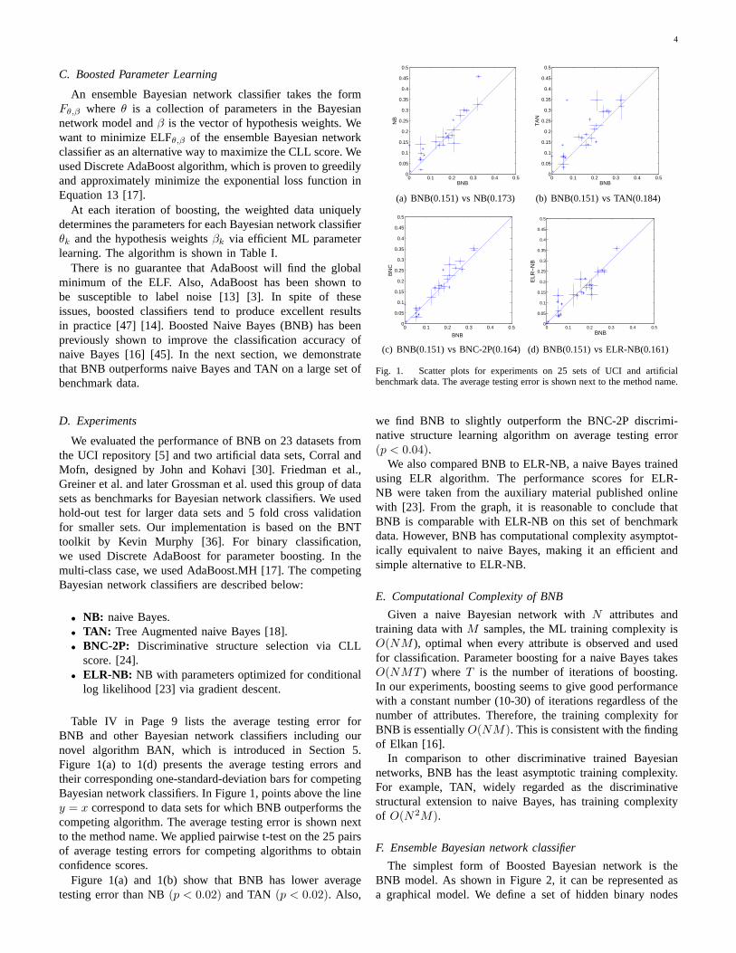
Table IV in Page 9 lists the average testing error forBNB and other Bayesian network classifiers including ournovel algorithm BAN, which is introduced in Section 5.Figure 1(a) to 1(d) presents the average testing errors andtheir corresponding one-standard-deviation bars for competingBayesian network classifiers. In Figure 1, points above the liney = x correspond to data sets for which BNB outperforms thecompeting algorithm. The average testing error is shown nextto the method name. We applied pairwise t-test on the 25 pairsof average testing errors for competing algorithms to obtainconfidence scores.

Figure 1(a) and 1(b) show that BNB has lower averagetesting error than NB(p < 0.02) and TAN (p < 0.02). Also,

0 0.1 0.2 0.3 0.4 0.50

0.05

0.1

0.15

0.2

0.25

0.3

0.35

0.4

0.45

0.5

BNB

NB

(a) BNB(0.151) vs NB(0.173)

0 0.1 0.2 0.3 0.4 0.50

0.05

0.1

0.15

0.2

0.25

0.3

0.35

0.4

0.45

0.5

BNB

TA

N

(b) BNB(0.151) vs TAN(0.184)

0 0.1 0.2 0.3 0.4 0.50

0.05

0.1

0.15

0.2

0.25

0.3

0.35

0.4

0.45

0.5

BNB

BN

C

(c) BNB(0.151) vs BNC-2P(0.164)

0 0.1 0.2 0.3 0.4 0.50

0.05

0.1

0.15

0.2

0.25

0.3

0.35

0.4

0.45

0.5

BNB

ELR

−N

B

(d) BNB(0.151) vs ELR-NB(0.161)

Fig. 1. Scatter plots for experiments on 25 sets of UCI and artificialbenchmark data. The average testing error is shown next to the method name.

we find BNB to slightly outperform the BNC-2P discrimi-native structure learning algorithm on average testing error(p < 0.04).

We also compared BNB to ELR-NB, a naive Bayes trainedusing ELR algorithm. The performance scores for ELR-NB were taken from the auxiliary material published onlinewith [23]. From the graph, it is reasonable to conclude thatBNB is comparable with ELR-NB on this set of benchmarkdata. However, BNB has computational complexity asymptot-ically equivalent to naive Bayes, making it an efficient andsimple alternative to ELR-NB.

E. Computational Complexity of BNB

Given a naive Bayesian network withN attributes andtraining data withM samples, the ML training complexity isO(NM ), optimal when every attribute is observed and usedfor classification. Parameter boosting for a naive Bayes takesO(NMT ) whereT is the number of iterations of boosting.In our experiments, boosting seems to give good performancewith a constant number (10-30) of iterations regardless of thenumber of attributes. Therefore, the training complexity forBNB is essentiallyO(NM). This is consistent with the findingof Elkan [16].

In comparison to other discriminative trained Bayesiannetworks, BNB has the least asymptotic training complexity.For example, TAN, widely regarded as the discriminativestructural extension to naive Bayes, has training complexityof O(N2M).

F. Ensemble Bayesian network classifier

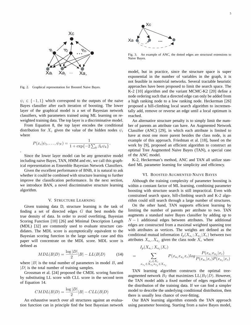
The simplest form of Boosted Bayesian network is theBNB model. As shown in Figure 2, it can be represented asa graphical model. We define a set of hidden binary nodes

5

Xa

1

Xc

Xa21 Xa

Ψ2 ...

...

Ψ Ψm

n

Fig. 2. Graphical representation for Boosted Naive Bayes.

ψi ∈ {−1, 1} which correspond to the outputs of the naiveBayes classifier after each iteration of boosting. The lowerlayer of the graphical model is a set of Bayesian networkclassifiers, with parameters trained using ML learning on re-weighted training data. The top layer is a discriminative model.

From Equation 8, the top layer encodes the conditionaldistribution forXc given the value of the hidden nodesψi

where

P (xc|ψ1, . . . , ψN ) =1

1 + exp{−2∑

k βkψk}.

.Since the lower layer model can be any generative model

including naive Bayes, TAN, HMM and etc, we call this graph-ical representation as Ensemble Bayesian Network Classifiers.

Given the excellent performance of BNB, it is natural to askwhether it could be combined with structure learning to furtherimprove the classification performance. In the next section,we introduce BAN, a novel discriminative structure learningalgorithm.

V. STRUCTURELEARNING

Given training data D, structure learning is the task offinding a set of directed edgesG that best models thetrue density of data. In order to avoid overfitting, BayesianScoring Function [10] [26] and Minimal Description Length(MDL) [32] are commonly used to evaluate structure can-didates. The MDL score is asymptotically equivalent to theBayesian scoring function in the large sample case and thispaper will concentrate on the MDL score. MDL score isdefined as

MDL(B|D) =log |D|

2|B| − LL(B|D) (14)

where|B| is the total number of parameters in modelB, and|D| is the total number of training samples.

Grossman et al. [24] proposed the CMDL scoring functionby substituting LL score with CLL score in the second termof Equation 14.

CMDL(B|D) =log |D|

2|B| − CLL(B|D)

An exhaustive search over all structures against an evalua-tion function can in principle find the best Bayesian network

Xa ...

Xc

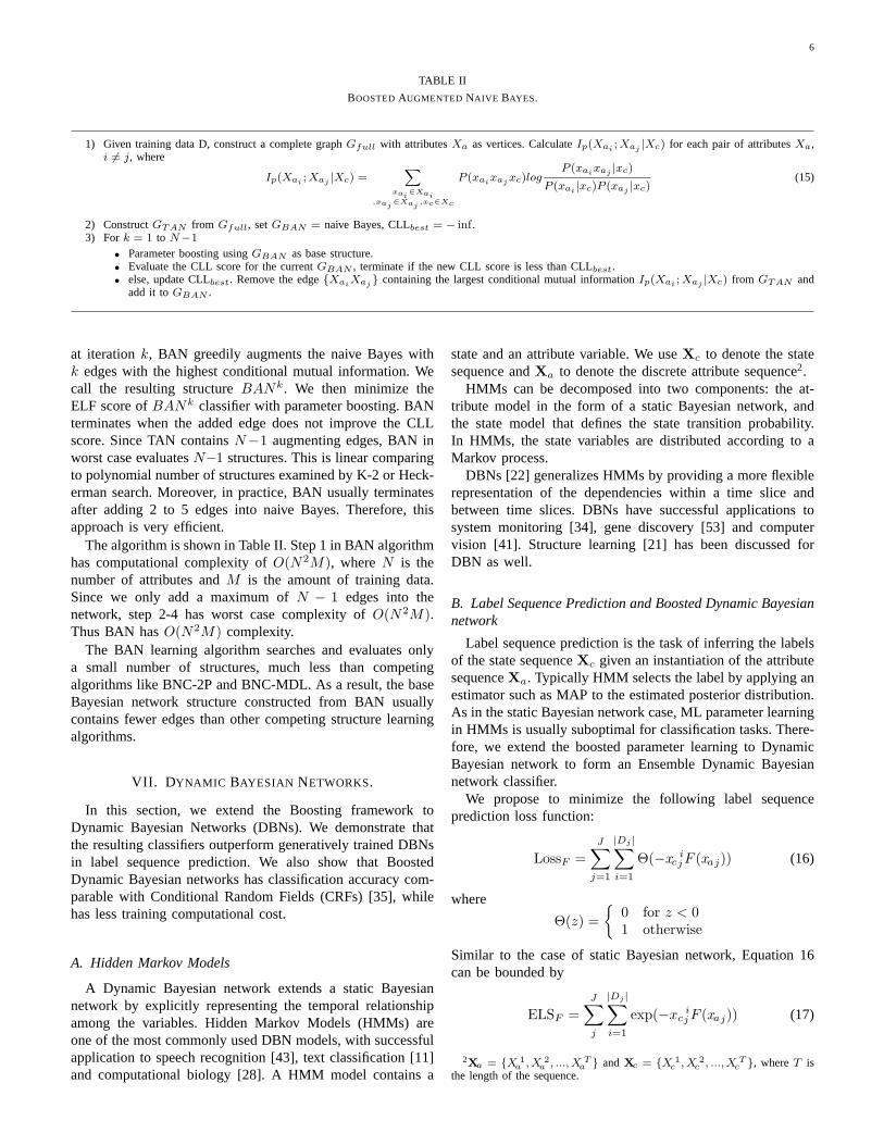
Fig. 3. An example of ANC, the dotted edges are structural extensions toNaive Bayes.

model, but in practice, since the structure space is superexponential in the number of variables in the graph, it isnot feasible in nontrivial networks. Several tractable heuristicapproaches have been proposed to limit the search space. TheK-2 [10] algorithm and the variant MCMC-K2 [20] define anode ordering such that a directed edge can only be added froma high ranking node to a low ranking node. Heckerman [26]proposed a hill-climbing local search algorithm to incremen-tally add, remove or reverse an edge until a local optimum isreached.

An alternative structure penalty is to simply limit the num-ber of parents an attribute can have. An Augmented NetworkClassifier (ANC) [29], in which each attribute is limited tohave at most one more parent besides the class node, is anexample of this approach. Friedman et al. [18], based on thework by [9], proposed an efficient algorithm to construct anoptimal Tree Augmented Naive Bayes (TAN), a special caseof the ANC model.

K-2, Heckerman’s method, ANC and TAN all utilize stan-dard ML parameter learning for simplicity and efficiency.

VI. B OOSTEDAUGMENTED NAIVE BAYES

Although the training complexity of parameter boosting iswithin a constant factor of ML learning, combining parameterboosting with structure search is still impractical. Even withconstrained search space, hill-climbing search and K-2 algo-rithm could still search through a large number of structures.

On the other hand, TAN supports efficient learning bylimiting the number of parents per attribute to two. TANaugments a standard naive Bayes classifier by adding up toN − 1 additional edges between attributes. The additionaledges are constructed from a maximal weighted spanning treewith attributes as vertices. The weights are defined as theconditional mutual informationIp(Xai

;Xaj|Xc) between two

attributesXai, Xaj

given the class nodeXc where

Ip(Xai;Xaj

|Xc)

=∑

xc∈Xcxai

∈Xaixaj

∈Xaj

P (xaixajxc)logP (xai

xaj|xc)

P (xai|xc)P (xaj

|xc)

TAN learning algorithm constructs the optimal tree-augmented networkBT that maximizesLL(BT |D). However,the TAN model adds a fixed number of edges regardless ofthe distribution of the training data. If we can find a simplermodel to describe the underlying conditional distribution, thenthere is usually less chance of over-fitting.

Our BAN learning algorithm extends the TAN approachusing parameter boosting. Starting from a naive Bayes model,

6

TABLE II

BOOSTEDAUGMENTED NAIVE BAYES.

1) Given training data D, construct a complete graphGfull with attributesXa as vertices. CalculateIp(Xai ; Xaj |Xc) for each pair of attributesXa,i 6= j, where

Ip(Xai ; Xaj |Xc) =∑

xai∈Xai

,xaj∈Xaj

,xc∈Xc

P (xaixaj xc)logP (xaixaj |xc)

P (xai |xc)P (xaj |xc)(15)

2) ConstructGTAN from Gfull, setGBAN = naive Bayes, CLLbest = − inf.3) For k = 1 to N−1

• Parameter boosting usingGBAN as base structure.• Evaluate the CLL score for the currentGBAN , terminate if the new CLL score is less than CLLbest.• else, update CLLbest. Remove the edge{XaiXaj } containing the largest conditional mutual informationIp(Xai ; Xaj |Xc) from GTAN and

add it toGBAN .

at iterationk, BAN greedily augments the naive Bayes withk edges with the highest conditional mutual information. Wecall the resulting structureBANk. We then minimize theELF score ofBANk classifier with parameter boosting. BANterminates when the added edge does not improve the CLLscore. Since TAN containsN−1 augmenting edges, BAN inworst case evaluatesN−1 structures. This is linear comparingto polynomial number of structures examined by K-2 or Heck-erman search. Moreover, in practice, BAN usually terminatesafter adding 2 to 5 edges into naive Bayes. Therefore, thisapproach is very efficient.

The algorithm is shown in Table II. Step 1 in BAN algorithmhas computational complexity ofO(N2M), whereN is thenumber of attributes andM is the amount of training data.Since we only add a maximum ofN − 1 edges into thenetwork, step 2-4 has worst case complexity ofO(N2M).Thus BAN hasO(N2M) complexity.

The BAN learning algorithm searches and evaluates onlya small number of structures, much less than competingalgorithms like BNC-2P and BNC-MDL. As a result, the baseBayesian network structure constructed from BAN usuallycontains fewer edges than other competing structure learningalgorithms.

VII. D YNAMIC BAYESIAN NETWORKS.

In this section, we extend the Boosting framework toDynamic Bayesian Networks (DBNs). We demonstrate thatthe resulting classifiers outperform generatively trained DBNsin label sequence prediction. We also show that BoostedDynamic Bayesian networks has classification accuracy com-parable with Conditional Random Fields (CRFs) [35], whilehas less training computational cost.

A. Hidden Markov Models

A Dynamic Bayesian network extends a static Bayesiannetwork by explicitly representing the temporal relationshipamong the variables. Hidden Markov Models (HMMs) areone of the most commonly used DBN models, with successfulapplication to speech recognition [43], text classification [11]and computational biology [28]. A HMM model contains a

state and an attribute variable. We useXc to denote the statesequence andXa to denote the discrete attribute sequence2.

HMMs can be decomposed into two components: the at-tribute model in the form of a static Bayesian network, andthe state model that defines the state transition probability.In HMMs, the state variables are distributed according to aMarkov process.

DBNs [22] generalizes HMMs by providing a more flexiblerepresentation of the dependencies within a time slice andbetween time slices. DBNs have successful applications tosystem monitoring [34], gene discovery [53] and computervision [41]. Structure learning [21] has been discussed forDBN as well.

B. Label Sequence Prediction and Boosted Dynamic Bayesiannetwork

Label sequence prediction is the task of inferring the labelsof the state sequenceXc given an instantiation of the attributesequenceXa. Typically HMM selects the label by applying anestimator such as MAP to the estimated posterior distribution.As in the static Bayesian network case, ML parameter learningin HMMs is usually suboptimal for classification tasks. There-fore, we extend the boosted parameter learning to DynamicBayesian network to form an Ensemble Dynamic Bayesiannetwork classifier.

We propose to minimize the following label sequenceprediction loss function:

LossF =J∑

j=1

|Dj |∑i=1

Θ(−xc ijF (xaj)) (16)

where

Θ(z) ={

0 for z < 01 otherwise

Similar to the case of static Bayesian network, Equation 16can be bounded by

ELSF =J∑j

|Dj |∑i=1

exp(−xcijF (xaj)) (17)

2Xa = {X 1a , X 2

a , ..., X Ta } andXc = {X 1

c , X 2c , ..., X T

c }, whereT isthe length of the sequence.

7

1) Given base DBN structure G andJ training sequenceD1,2,...,J , whereDj = {xa1j , xc

1j , xa

2j , xc

2j , . . . , xa

|Dj |j , xc

|Dj |j }.

2) Initialize data weightsW with uniform distribution across all samples,wij = 1/N, i = 1, 2, . . . , |Dj | whereN =

J∑i=1

|Di|.

3) Repeat fork = 1, 2, . . . , K

a) θk is learnt through maximum likelihood parameter learning on the weighted dataDw.

b) Compute the combined weighted label error for the training sequences,errk = Ew[1xc 6=fθk(xa)] =

∑i,j w i

j

[1xc

ij 6=fθk

(xaj)

]c) βk = 0.5log 1−errk

errk

d) Update weightsw ij = w i

j exp{βkxcij fθk

(xaj)} and normalize.

4) Ensemble output: signK∑

k=1βkfθk

(xa)

TABLE IIIBOOST-DBN TRAINS AN ENSEMBLE DYNAMIC BAYESIAN NETWORK CLASSIFIER TO IMPROVE LABEL PREDICTION ACCURACY.

Given the weak classifierfk(xa) at each iteration of boosting,we can see, with easy modification to the proof for Result1in [17], that Discrete AdaBoost (Population version) greedilyand approximately maximizes Equation 17 by setting thehypothesis weightsβ as:

βk = 0.5 log1 − errkerrk

where

errk = Ew[1xc 6=fθk(xa)] =

∑i,j

w ij

[1xc

ij 6=fθk

(xaj)

].

The Boosted DBN parameter learning algorithm is shown inTable III.

Step 3(a) in Table III has computational complexity ofO(NM + C2M), where C is the cardinality of the statespace. This is essentially optimal when every feature is usedfor classification in HMM. Step 3(b) evaluates the givenDBN via Forward-Backward algorithm with computationalcomplexity of O(C2NM). The computational complexityfor Boost-DBN parameter learning algorithm is thereforeO(C2NMT ), whereT is the number of boosting iteration. Inour experiments, Boosted DBN parameter learning algorithmconverges after 25-30 iterations of boosting.

VIII. E XPERIMENTS

The experiments section is organized into three subsections.Subsection A through C contain experiments and analysisof BAN structure learning algorithm. Subsection D containsexperiments and analysis for Boost-DBN algorithm.

A. Experiments on BAN with simulated datasets

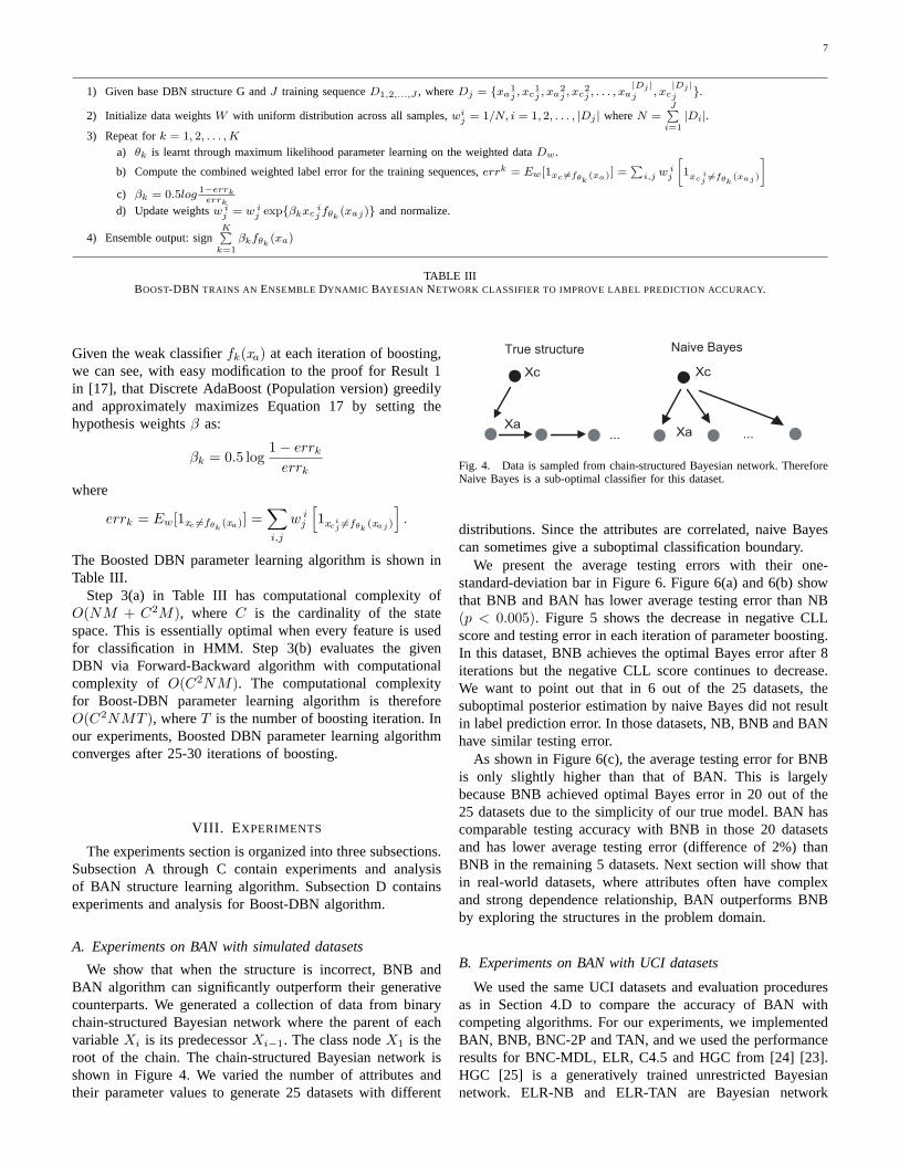
We show that when the structure is incorrect, BNB andBAN algorithm can significantly outperform their generativecounterparts. We generated a collection of data from binarychain-structured Bayesian network where the parent of eachvariableXi is its predecessorXi−1. The class nodeX1 is theroot of the chain. The chain-structured Bayesian network isshown in Figure 4. We varied the number of attributes andtheir parameter values to generate 25 datasets with different

Xa

Xc Xc

True structure Naive Bayes

Xa... ...

Fig. 4. Data is sampled from chain-structured Bayesian network. ThereforeNaive Bayes is a sub-optimal classifier for this dataset.

distributions. Since the attributes are correlated, naive Bayescan sometimes give a suboptimal classification boundary.

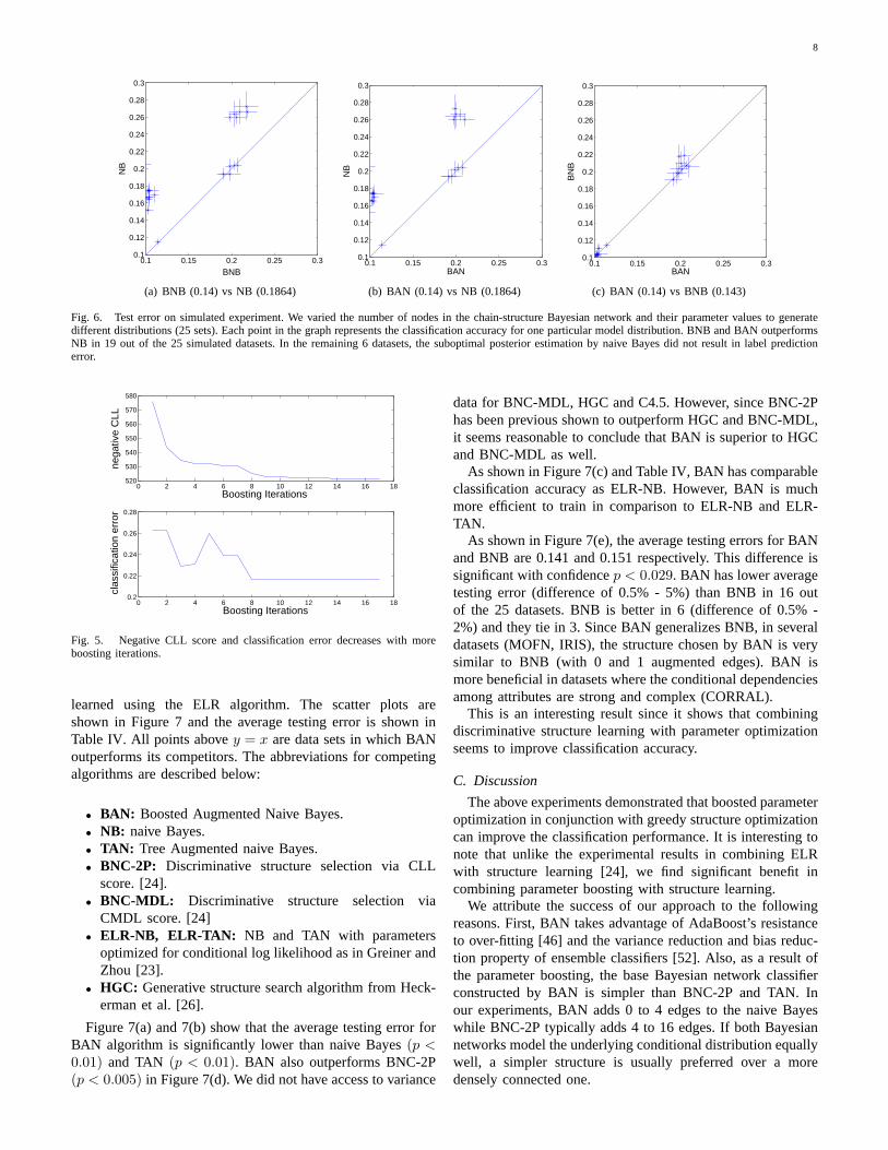
We present the average testing errors with their one-standard-deviation bar in Figure 6. Figure 6(a) and 6(b) showthat BNB and BAN has lower average testing error than NB(p < 0.005). Figure 5 shows the decrease in negative CLLscore and testing error in each iteration of parameter boosting.In this dataset, BNB achieves the optimal Bayes error after 8iterations but the negative CLL score continues to decrease.We want to point out that in 6 out of the 25 datasets, thesuboptimal posterior estimation by naive Bayes did not resultin label prediction error. In those datasets, NB, BNB and BANhave similar testing error.

As shown in Figure 6(c), the average testing error for BNBis only slightly higher than that of BAN. This is largelybecause BNB achieved optimal Bayes error in 20 out of the25 datasets due to the simplicity of our true model. BAN hascomparable testing accuracy with BNB in those 20 datasetsand has lower average testing error (difference of 2%) thanBNB in the remaining 5 datasets. Next section will show thatin real-world datasets, where attributes often have complexand strong dependence relationship, BAN outperforms BNBby exploring the structures in the problem domain.

B. Experiments on BAN with UCI datasets

We used the same UCI datasets and evaluation proceduresas in Section 4.D to compare the accuracy of BAN withcompeting algorithms. For our experiments, we implementedBAN, BNB, BNC-2P and TAN, and we used the performanceresults for BNC-MDL, ELR, C4.5 and HGC from [24] [23].HGC [25] is a generatively trained unrestricted Bayesiannetwork. ELR-NB and ELR-TAN are Bayesian network

8

0.1 0.15 0.2 0.25 0.30.1

0.12

0.14

0.16

0.18

0.2

0.22

0.24

0.26

0.28

0.3

BNB

NB

(a) BNB (0.14) vs NB (0.1864)

0.1 0.15 0.2 0.25 0.30.1

0.12

0.14

0.16

0.18

0.2

0.22

0.24

0.26

0.28

0.3

BAN

NB

(b) BAN (0.14) vs NB (0.1864)

0.1 0.15 0.2 0.25 0.30.1

0.12

0.14

0.16

0.18

0.2

0.22

0.24

0.26

0.28

0.3

BAN

BN

B

(c) BAN (0.14) vs BNB (0.143)

Fig. 6. Test error on simulated experiment. We varied the number of nodes in the chain-structure Bayesian network and their parameter values to generatedifferent distributions (25 sets). Each point in the graph represents the classification accuracy for one particular model distribution. BNB and BAN outperformsNB in 19 out of the 25 simulated datasets. In the remaining 6 datasets, the suboptimal posterior estimation by naive Bayes did not result in label predictionerror.

0 2 4 6 8 10 12 14 16 18520

530

540

550

560

570

580

nega

tive

CLL

Boosting Iterations

0 2 4 6 8 10 12 14 16 180.2

0.22

0.24

0.26

0.28

clas

sific

atio

n er

ror

Boosting Iterations

Fig. 5. Negative CLL score and classification error decreases with moreboosting iterations.

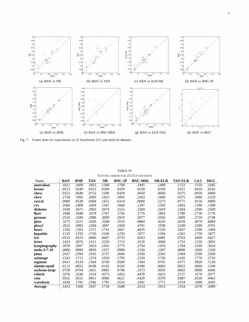
learned using the ELR algorithm. The scatter plots areshown in Figure 7 and the average testing error is shown inTable IV. All points abovey = x are data sets in which BANoutperforms its competitors. The abbreviations for competingalgorithms are described below:

• BAN: Boosted Augmented Naive Bayes.• NB: naive Bayes.• TAN: Tree Augmented naive Bayes.• BNC-2P: Discriminative structure selection via CLL

score. [24].• BNC-MDL: Discriminative structure selection via

CMDL score. [24]• ELR-NB, ELR-TAN: NB and TAN with parameters

optimized for conditional log likelihood as in Greiner andZhou [23].

• HGC: Generative structure search algorithm from Heck-erman et al. [26].

Figure 7(a) and 7(b) show that the average testing error forBAN algorithm is significantly lower than naive Bayes(p <0.01) and TAN (p < 0.01). BAN also outperforms BNC-2P(p < 0.005) in Figure 7(d). We did not have access to variance

data for BNC-MDL, HGC and C4.5. However, since BNC-2Phas been previous shown to outperform HGC and BNC-MDL,it seems reasonable to conclude that BAN is superior to HGCand BNC-MDL as well.

As shown in Figure 7(c) and Table IV, BAN has comparableclassification accuracy as ELR-NB. However, BAN is muchmore efficient to train in comparison to ELR-NB and ELR-TAN.

As shown in Figure 7(e), the average testing errors for BANand BNB are 0.141 and 0.151 respectively. This difference issignificant with confidencep < 0.029. BAN has lower averagetesting error (difference of 0.5% - 5%) than BNB in 16 outof the 25 datasets. BNB is better in 6 (difference of 0.5% -2%) and they tie in 3. Since BAN generalizes BNB, in severaldatasets (MOFN, IRIS), the structure chosen by BAN is verysimilar to BNB (with 0 and 1 augmented edges). BAN ismore beneficial in datasets where the conditional dependenciesamong attributes are strong and complex (CORRAL).

This is an interesting result since it shows that combiningdiscriminative structure learning with parameter optimizationseems to improve classification accuracy.

C. Discussion

The above experiments demonstrated that boosted parameteroptimization in conjunction with greedy structure optimizationcan improve the classification performance. It is interesting tonote that unlike the experimental results in combining ELRwith structure learning [24], we find significant benefit incombining parameter boosting with structure learning.

We attribute the success of our approach to the followingreasons. First, BAN takes advantage of AdaBoost’s resistanceto over-fitting [46] and the variance reduction and bias reduc-tion property of ensemble classifiers [52]. Also, as a result ofthe parameter boosting, the base Bayesian network classifierconstructed by BAN is simpler than BNC-2P and TAN. Inour experiments, BAN adds 0 to 4 edges to the naive Bayeswhile BNC-2P typically adds 4 to 16 edges. If both Bayesiannetworks model the underlying conditional distribution equallywell, a simpler structure is usually preferred over a moredensely connected one.

9

0 0.1 0.2 0.3 0.4 0.50

0.05

0.1

0.15

0.2

0.25

0.3

0.35

0.4

0.45

0.5

BAN

NB

(a) BAN vs NB

0 0.1 0.2 0.3 0.4 0.50

0.05

0.1

0.15

0.2

0.25

0.3

0.35

0.4

0.45

0.5

BANT

AN

(b) BAN vs TAN

0 0.1 0.2 0.3 0.4 0.50

0.05

0.1

0.15

0.2

0.25

0.3

0.35

0.4

0.45

0.5

BAN

ELR

−N

B

(c) BAN vs ELR-NB

0 0.1 0.2 0.3 0.4 0.50

0.05

0.1

0.15

0.2

0.25

0.3

0.35

0.4

0.45

0.5

BAN

BN

C

(d) BAN vs BNC-2P

0 0.1 0.2 0.3 0.4 0.50

0.05

0.1

0.15

0.2

0.25

0.3

0.35

0.4

0.45

0.5

BAN

BN

B

(e) BAN vs BNB

0 0.1 0.2 0.3 0.4 0.50

0.05

0.1

0.15

0.2

0.25

0.3

0.35

0.4

0.45

0.5

BAN

BN

C−

MD

L

(f) BAN vs BNC-MDL

0 0.1 0.2 0.3 0.4 0.50

0.05

0.1

0.15

0.2

0.25

0.3

0.35

0.4

0.45

0.5

BANE

LR−

TA

N

(g) BAN vs ELR-TAN

0 0.1 0.2 0.3 0.4 0.5 0.6 0.70

0.1

0.2

0.3

0.4

0.5

0.6

BAN VS HGC

BAN

HG

C

(h) BAN vs HGC

Fig. 7. Scatter plots for experiments on 25 benchmark UCI and artificial datasets.

TABLE IV

TESTING ERROR FOR25 UCI DATASETS

Name BAN BNB TAN NB BNC-2P BNC-MDL NB-ELR TAN-ELR C4.5 HGCaustralian .1812 .1609 .1855 .1368 .1768 .1405 .1488 .1723 .1510 .1445breast .0513 .0549 .0312 .0200 .0330 .0518 .0339 .0351 .0610 .0245chess .0253 .0640 .0753 .1180 .0428 .0450 .0600 .0375 .0050 .0469cleve .1758 .1995 .2095 .1825 .2095 .2563 .1660 .0375 .2060 .2129corral .0000 .0538 .0468 .1412 .0314 .0000 .1273 .0771 .0150 .0000crx .1684 .1408 .1669 .1347 .1684 .1397 .1505 .1603 .1390 .1308diabetes .2438 .2675 .2903 .2974 .2553 .2569 .2419 .2384 .2590 .2569flare .1698 .1848 .1679 .1707 .1726 .1776 .1803 .1780 .1730 .1776german .2510 .2580 .2980 .3000 .2910 .2977 .2456 .2409 .2710 .2748glass .3175 .3221 .3456 .3268 .3535 .6884 .4220 .5018 .4070 .6884glass2 .2023 .2083 .2269 .2087 .2269 .4701 .1938 .2249 .2390 .4701heart .1556 .1593 .1371 .1741 .1667 .4635 .1550 .1847 .2180 .1484hepatitis .1125 .1250 .1750 .1500 .1250 .1877 .1294 .1302 .1750 .1877iris .0533 .0533 .0800 .0667 .0733 .0563 .0485 .0763 .0400 .0427letter .1433 .2076 .1511 .2520 .1712 .3530 .3068 .1752 .1220 .3092lymphography .2078 .2097 .3453 .1452 .2775 .2794 .1470 .1784 .2160 .3624mofn-3-7-10 .0000 .0000 .0830 .1357 .0908 .1328 .1367 .0000 .1600 .1328pima .2427 .2394 .2916 .2737 .2606 .2569 .2505 .2384 .2590 .2569satimage .1543 .1712 .1374 .1920 .1795 .2220 .1730 .1420 .1770 .2710segment .0415 .0510 .1364 .0740 .0500 .1364 .0701 .0571 .0820 .1130shuttle-small .0113 .0052 .0108 .0142 .0102 .0186 .0083 .0052 .0060 .1349soybean-large .0758 .0704 .3451 .0885 .0746 .3373 .0920 .0663 .0890 .6466vehicle .3276 .3246 .3154 .4573 .3452 .4478 .3453 .2727 .3170 .5077vote .0552 .0552 .0851 .0966 .0621 .0420 .0370 .0487 .0530 .0463waveform .1630 .1785 .2566 .1795 .2516 .3281 .1772 .2534 .3490 .4345Average .1412 .1506 .1837 .1734 .1640 .2314 .1613 .1554 .1676 .2409

10

Frontal

Speech

Frontal

Speech Skin

Lip motion

Sound

Frontal Speech

Face

Frontal

Transition Model

Sensors

Feature Model

Sensors Sensors

...

Transition Model Feature Model

PlayerState

PlayerState Player

State

PlayerState Player

State

PlayerState

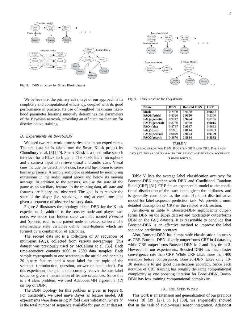
Fig. 8. DBN structure for Smart Kiosk dataset

We believe that the primary advantage of our approach is itssimplicity and computational efficiency, coupled with its goodperformance in practice. Its use of weighted maximum likeli-hood parameter learning uniquely determines the parametersof the Bayesian network, providing an efficient mechanism fordiscriminative training.

D. Experiments on Boost-DBN

We used two real-world time-series data in our experiments.The first data set is taken from the Smart Kiosk project byChoudhury et al. [8] [40]. Smart Kiosk is a open-mike speechinterface for a Black Jack game. The kiosk has a microphoneand a camera input to retrieve visual and audio cues. Visualcues include the detection of skin, face and lip-motion to sensehuman presence. A simple audio cue is obtained by monitoringexcursions in the audio signal above and below its movingaverage. In addition to the sensors, we use the state of thegame as an auxiliary feature. In the training data, all state andfeatures are binary and observed. The goal is to recover thestate of the player (i.e. speaking or not) at each time slicegiven a sequence of observed sensory data.

Figure 8 illustrates the topology of the DBN for the Kioskexperiment. In addition to the sensory node and player statenode, we added two hidden state variables namedFrontalandSpeech, each is the parent node of related sensors. Theintermediate state variables define meta-features which areformed by a combination of attributes.

The second data set is a collection of 37 sequences ofmulti-part FAQs, collected from various newsgroups. Thisdataset was previously used by McCallum et al. [35]. Eachtime-sequence contains 1000 to 2500 data samples. Eachsample corresponds to one sentence in the article and contains20 binary features and a state label for the topic of thesentence (introduction, question, answer or conclusion). Forthis experiment, the goal is to accurately recover the state labelsequence given a instantiation of feature sequences. Since thisis a 4 class problem, we used Adaboost.MH algorithm [17]on top of DBN.

The DBN topology for this problem is given in Figure 9.For tractability, we used naive Bayes as feature model. Allexperiments were done usingN fold cross validation, whereNis the total number of sequence available for particular dataset.

Sentence Category

Contains Number

Sentence Category

Attributes

Sentence Category

Sentence Category

Attributes

Attributes

Transition Model

Feature Model

Sentence Category

Sentence Category

Transition Model Feature Model

Contains HTTP

Indented

...

...

Fig. 9. DBN structure for FAQ dataset

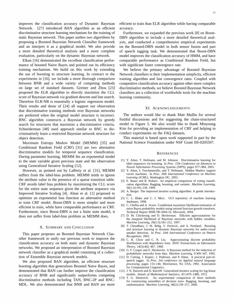
Name DBN Boosted DBN CRFkiosk 0.7490 0.9120 0.9641FAQ1(fetish) 0.8330 0.9156 0.8300FAQ2(genetic) 0.9242 0.9464 0.8756FAQ3(general) 0.8750 0.8960 0.9015FAQ4(aix) 0.8767 0.9047 0.8663FAQ5(bsd) 0.7981 0.8174 0.8033FAQ6(neural) 0.9049 0.9173 0.9129FAQ7(acorn) 0.8870 0.8884 0.8882

TABLE V

TESTING ERROR FORDBN, BOOSTEDDBN AND CRF. FOR EACH

DATASET, THE ALGORITHM WITH THE BEST CLASSIFICATION ACCURACY

IS HIGHLIGHTED.

Table V lists the average label classification accuracy forBoosted-DBN together with DBN and Conditional RandomField (CRF) [31]. CRF fits an exponential model to the condi-tional distribution of the state labels given the attributes, andis generally considered as the state-of-the-art discriminativemodel for label sequence prediction task. We provide a moredetailed description of CRF in the related work section.

As shown in Table V, Boosted-DBN significantly outper-forms DBN on the Kiosk dataset and moderately outperformsDBN on the FAQ datasets. It is reasonable to conclude thatBoosted-DBN is an effective method to improve the labelsequence prediction accuracy.

Also, Boosted-DBN has comparable classification accuracyas CRF. Boosted-DBN slightly outperforms CRF in 4 datasets,while CRF outperforms Boosted-DBN in 2 and they tie in 2.However, in our experiments, Boosted-DBN has much fasterconvergence rate than CRF. While CRF takes more than 400iteration before convergence, Boosted-DBN takes only 10-30 iterations to get good classification accuracy. Since eachiteration of CRF training has roughly the same computationalcomplexity as one boosting iteration for Boost-DBN, Boost-DBN has less training computational complexity.

IX. RELATED WORK

This work is an extension and generalization of our previousworks [8] [39] [27]. In [8] [39], we empirically showedthat in the task of audio-visual sensor integration, AdaBoost

11

improves the classification accuracy of Dynamic BayesianNetwork. [27] introduced BAN algorithm as an efficientdiscriminative structure learning mechanism for the training ofstatic Bayesian network. This paper unifies two algorithms byproposing a Boosted Bayesian Network Classifier frameworkand an interpret it as a graphical model. We also providea more detailed theoretical analysis and a more completeevaluation, particularly on the dynamic Bayesian network.

Elkan [16] demonstrated the excellent classification perfor-mance of boosted Naive Bayes and pointed out its efficiencytraining mechanism. We build on this work by extendingthe use of boosting to structure learning. In contract to theexperiments in [16], we include a more thorough comparisonbetween BNB and a wide variety of competing methodson large set of standard datasets. Greiner and Zhou [23]proposed the ELR algorithm to directly maximize the CLLscore of Bayesian network via gradient descent and line search.Therefore ELR-NB is essentially a logistic regression model.Their results and those of [24] all support our observationthat discriminative training methods over Bayesian networksare preferred when the original model structure is incorrect.BNC algorithm constructs a Bayesian network by greedysearch for structures that maximize a discriminative criteria.Schneiderman [48] used approach similar to BNC to dis-criminatively learn a restricted Bayesian network structure forobject detection.

Maximum Entropy Markov Model (MEMM) [35] andConditional Random Field (CRF) [31] are two alternativediscriminative models for temporal sequence classification.During parameter learning, MEMM fits an exponential modelto the state variable given previous state and the observationusing Generalized Iterative Scaling [12].

However, as pointed out by Lafferty et al. [31], MEMMsuffers from the label-bias problem. MEMM tends to ignorethe attribute value in the presence of a sparse transition table.CRF avoids label bias problem by maximizing the CLL scorefor the entire state sequence given the attribute sequence viaImproved Iterative Scaling [4]. Altun et al. [1] proposed tooptimize an exponential loss function an alternative methodto train CRF model. Boost-DBN is more simpler and moreefficient to train, while have comparable performance as CRF.Furthermore, since Boost-DBN is not a finite state model, itdoes not suffer from label-bias problem as MEMM does.

X. SUMMARY AND CONCLUSION

This paper proposes an Boosted Bayesian Network Clas-sifier framework to unify our previous work to improve theclassification accuracy on both static and dynamic Bayesiannetworks. We proposed an interpretation of Boosted Bayesiannetwork classifier as a graphical model consisting of a collec-tion of Ensemble Bayesian network models.

We also proposed BAN algorithm, an efficient structurelearning algorithm that generalizes Boosted Naive Bayes, anddemonstrated that BAN can further improve the classificationaccuracy of BNB and significantly outperforms competingdiscriminative methods including TAN, BNC-2P and BNC-MDL. We also demonstrated that BNB and BAN are more

efficient to train than ELR algorithm while having comparableaccuracy.

Furthermore, we expanded the previous work [8] on Boost-DBN algorithm to include a more detailed theoretical anal-ysis, and conducted a comprehensive empirical experimentson the Boosted-DBN model in both sensor fusion and partof speech tagging task. We demonstrated that Boost-DBNmodel improves the classification accuracy of HMM, and havecomparable performance as Conditional Random Field, butwith significant faster convergence rate.

We believe the primary advantage of Boosted BayesianNetwork classifiers is their implementation simplicity, efficienttraining algorithm and fast convergence rates. Coupled withcompetitive classification accuracy against other more complexdiscriminative methods, we believe Boosted Bayesian Networkclassifiers are a collection of worthwhile tools for the machinelearning community.

XI. A CKNOWLEDGEMENTS

The authors would like to thank Matt Mullin for severalfruitful discussions and for suggesting the chain-structuredmodel in Figure 5. We also would like to thank MinyoungKim for providing an implementation of CRF and helping toconduct experiments on the FAQ datasets.

This material is based upon work supported in part by theNational Science Foundation under NSF Grant IIS-0205507.

REFERENCES

[1] Y. Altun, T. Hofmann, and M. Johnson. Discriminative learning forlabel sequences via boosting. InProc. 15th Conference on Advances inNeural Information Processing Systems (NIPS), pages 977–984, 2003.

[2] Y. Altun, I. Tsochantaridis, and T. Hofmann. Hidden Markov supportvector machines. InProc. 20th International Conference on MachineLearning (ICML), Washington DC, 2003.

[3] E. Bauer and R. Kohavi. An empirical comparison of voting classifi-cation algorithms: Bagging, boosting, and variants.Machine Learning,36(1-2):105–139, 1999.

[4] A. Berger. The improved iterative scaling algorithm: A gentle introduc-tion.

[5] C. L. Blake and C. J. Merz. UCI repository of machine learningdatabases, 1998.

[6] C. Chelba and A. Acero. Conditional maximum likelihood estimation ofnaive Bayes probability models using rational function growth transform.Technical Report MSR-TR-2004-33, Microsoft, 2004.

[7] D. M. Chickering and D. Heckerman. Efficient approximations forthe marginal likelihood of Bayesian networks with hidden variables.Machine Learning, 29(2-3):181–212, 1997.

[8] T. Choudhury, J. M. Rehg, V. Pavlovic, and A. Pentland. Boostingand structure learning in dynamic Bayesian networks for audio-visualspeaker detection. InProc. 16th International Conference on PatternRecognition, 2002.

[9] C. K. Chow and C. N. Liu. Approximating discrete probabilitydistributions with dependence trees.IEEE Transactions on InformationTheory, 14(3):462–467, 1968.

[10] G. F. Cooper and E. Herskovits. A Bayesian method for the induction ofprobabilistic networks from data.Machine Learning, 9:309–347, 1992.

[11] D. Cutting, J. Kupiec, J. Pedersen, and P. Sibun. A practical part-of-speech tagger. InProc. 3rd conference on Applied natural languageprocessing, pages 133–140, Morristown, NJ, USA, 1992. Associationfor Computational Linguistics.

[12] J. N. Darroch and D. Ratcliff. Generalized iterative scaling for log-linearmodels.Annals of Mathematical Statistics, 43:1470–1480, 1972.

[13] T. G. Dietterich. An experimental comparison of three methodsfor constructing ensembles of decision trees: Bagging, boosting, andrandomization.Machine Learning, 40(2):139–157, 2000.

12

[14] H. Drucker and C. Cortes. Boosting Decision Trees. InProc. 8thAdvances in Neural Information Processing Systems (NIPS), pages 470–485. 1996.

[15] R. O. Duda and P. E. Hart.Pattern Classification and Scene Analysis.Wiley-Interscience Publication, New York, 1973.

[16] C. Elkan. Boosting and naive Bayesian learning. Technical report,Department of Computer Science and Engineering, University of Cali-fornia, San Diego., 1997.

[17] J. Friedman, T. Hastie, and R. Tibshirani. Additive logistic regression:a statistical view of boosting.The Annals of Statistics, 38(2):337–374,2000.

[18] N. Friedman, D. Geiger, and M. Goldszmidt. Bayesian networkclassifiers.Machine Learning, 29:131–163, 1997.

[19] N. Friedman, L. Getoor, D. Koller, and A. Pfeffer. Learning probabilisticrelational models. InProc. 16th International Joint Conf. on ArtificialIntelligence (IJCAI), pages 1300–1309, 1999.

[20] N. Friedman and D. Koller. Being Bayesian about network structure. InProc. 16th Conference on Uncertainty in Artificial Intelligence (UAI),pages 201–210, June 2000.

[21] N. Friedman, K. Murphy, and S. Russell. Learning the structure of dy-namic probabilistic networks. InProc. 14th Conference on Uncertaintyin Artificial Intelligence (UAI), pages 139–147, San Francisco, 1998.

[22] Z. Ghahramani. Learning dynamic Bayesian networks.AdaptiveProcessing of Sequences and Data Structures . Lecture Notes in ArtificialIntelligence, 1387:168–187, 1998.

[23] R. Greiner and W. Zhou. Structural extension to logistic regression: Dis-criminative parameter learning of belief net classifiers. InProceedings ofannual meeting of the American Association for Artificial Intelligence,pages 167–173, 2002.

[24] D. Grossman and P. Domingos. Learning Bayesian network classifiersby maximizing conditional likelihood. InProc. 21st International Con-ference on Machine Learning (ICML), pages 361–368, Banff, Canada,2004. ACM Press.

[25] D. Heckerman. A tutorial on learning with bayesian networks. TechnicalReport MSR-TR-95-06, Microsoft Reserach, 1995.

[26] D. Heckerman, D. Geiger, and D.M. Chickering. Learning Bayesiannetworks: The combination of knowledge and statistical data.MachineLearning, 20(3):197–243, 1995.

[27] Y. Jing, V. Pavlovic, and J. M. Rehg. Efficient discriminative learningof Bayesian network classifiers via boosted augmented naive Bayes. In[Accepted for publication]Proc. 22nd International Conf. on MachineLearning (ICML), 2005.

[28] V. Jojic, N. Jojic, C. Meek, D. Geiger, A. Siepel, D. Haussler, andD. Heckerman. Efficient approximations for learning phylogeneticHMM models from data.Bioinformatics, 20(1):161–168, 2004.

[29] E. Keogh and M. Pazzani. Learning augmented Bayesian classifiers: Acomparison of distribution-based and classification-based approaches. InProc. 7th International Workshop on Artificial Intelligence and Statistics,pages 225–230, 1999.

[30] R. Kohavi and G. H. John. Wrappers for feature subset selection.Artificial Intelligence, 97(1-2):273–324, 1997.

[31] J. Lafferty, A. McCallum, and F. Pereira. Conditional random fields:Probabilistic models for segmenting and labeling sequence data. InProc.18th International Conf. on Machine Learning (ICML), pages 282–289,2001.

[32] W. Lam and F. Bacchus. Learning Bayesian belief networks. an approachbased on the mdl principle.Computational Intelligence, 10:269–293.

[33] P. Langley, W. Iba, and K. Thompson. An analysis of Bayesianclassifiers. InProceedings of the Tenth National Conference on ArtificialIntelligence, pages 223–228, San Jose, CA, 1992. AAAI Press.

[34] U. Lerner, B. Moses, S. Maricia, S. McIlraith, and D. Koller. Monitoringa complez physical system using a hybrid dynamic Bayes net. InProceedings of the 18th Annual Conference on Uncertainty in ArtificialIntelligence (UAI-02), pages 301–310, San Francisco, CA, 2002. MorganKaufmann Publishers.

[35] A. McCallum, D. Freitag, and F. Pereira. Maximum entropy Markovmodels for information extraction and segmentation. InProc. 17thInternational Conference on Machine Learning (ICML), pages 591–598,San Francisco, CA, 2000.

[36] K. Murphy. The Bayes net toolbox for matlab.Computing Science andStatistics, 33, 2001.

[37] A. Y. Ng and M. I. Jordan. On discriminative vs. generative classifiers:A comparison of logistic regression and naive Bayes. InProc. 14thConference on Advances in Neural Information Processing Systems(NIPS), pages 841–848, 2002.

[38] V. Pavlovic, A. Garg, and S. Kasif. A Bayesian framework for combininggene predictions.Bioinformatics, 18(1):19–27, 2002.

[39] V. Pavlovic, A. Garg, and J. M. Rehg. Boosted learning in dynamicBayesian networks for multimodal speaker detection.Proceedings ofthe IEEE, 91(9):1355–1369, 2003.

[40] V. Pavlovic, A. Garg, J. M. Rehg, and T. Huang. Multimodal speakerdetection using error feedback dynamic Bayesian networks. In2000IEEE Computer Society Conference on Computer Vision and PatternRecognition (CVPR), volume 2, pages 34–41, 2000.

[41] V. Pavlovic, J. M. Rehg, T. Cham, and K. P. Mu rphy. A dynamicbayesian network approach to figure tracking using learned dy namicmodels. InIntl. Conf. on Computer Vision, 1999.

[42] J. Pearl. Probabilistic Reasoning in Intelligent Systems: Networks ofPlausible Inference.Morgan Kaufmann, 1988.

[43] L. Rabiner and B.H. Juang.Fundamentals of Speech Recognition.Prentice Hall, Englewood Cliffs, NJ, 1993.

[44] J. M. Rehg, V. Pavlovic, T. S. Huang, and W. T. Freeman.SpecialSection on Graphical models in Computer Vision, IEEE Transactionson Pattern Analysis and Machine Intelligence, 25(7), 2003.

[45] G. Ridgeway, D. Madigan, T. Richardson, and J. O’Kane. Interpretableboosted naive Bayes classification. InProc. 4th International Conferenceon Knowledge Discovery and Data Mining, 1998.

[46] R. E. Schapire and Y. Singer. Improved boosting algorithms usingconfidence-rated predictions. InProc. 11th Annual Conference onComputational Learning Theory, 1998.

[47] R. E. Schapire and Y. Singer. BoosTexter: A boosting-based system fortext categorization.Machine Learning, 39(2/3):135–168, 2000.

[48] H. Schneiderman. Learning a restricted Bayesian network for objectdetection. InProc. Computer Society Conference on Computer Visionand Pattern Recognition (CVPR), pages 639–646, June 2004.

[49] E. Segal, R. Yelensky, and D. Koller. Genome-wide discovery oftranscriptional modules from dna sequence and gene expression.Bioin-formatics, 19(1):273–82, 2003.

[50] B. Taskar, C. Guestrin, and D. Koller. Max-margin Markov networks. InProc. 16th Conference on Advances in Neural Information ProcessingSystems (NIPS), Cambridge, MA, 2004. MIT Press.

[51] A. Torralba, K. P. Murphy, and W. T. Freeman. Sharing features:efficient boosting procedures for multiclass object detection. InProc.IEEE Conference on Computer Vision and Pattern Recognition (CVPR),volume 2, pages 762–769, Washington, DC, June 2004.

[52] G. Webb and Z. Zheng. Multistrategy ensemble learning: Reducingerror by combining ensemble learning techniques.IEEE Transactionson Knowledge and Data Engineering, 16(8):980–991, August 2004.

[53] M. Zou and S. D. Conzen. A new dynamic Bayesian network (DBN)approach for identifying gene regulatory networks from time coursemicroarray data.Bioinformatics, 21(1):71–79, 2005.