book excerpt english

Elektor Electronics

www.elektor-electronics.co.uk

ISBN 978-0-905705-71-2

Ped

ram

Aza

d, T

ilo G

ock

el, R

üd

iger

Dill

man

n

Pedram Azad, Tilo Gockel, Rüdiger Dillmann

Com

pute

r V

isio

n

Computer VisionPrinciples and Practice

Pedram Azad, Tilo Gockel, Rüdiger Dillmann

Computer Vision Principles and Practice

Computer vision is probably the most exciting branch of image processing,

and the number of applications in robotics, automation technology and

quality control is constantly increasing. Unfortunately entering this research

area is, as yet, not simple. Those who are interested must fi rst go through

a lot of books, publications and software libraries.

With this book, however, the fi rst step is easy. The theoretically well-founded

content is understandable and is supplemented by many practical examples. Source code is provided

with the specially developed platform-independent open source library IVT in the programming language

C/C++. The use of the IVT is not necessary, but it does make for a much easier entry and allows fi rst

developments to be quickly produced.

The authorship is made up of research assistants of the chair of Professor

Rüdiger Dillmann at the Institut für Technische Informatik (ITEC),

Universität Karlsruhe (TH). Having gained extensive experience in image

processing in many research and industrial projects, they are now passing

this knowledge on.

Among other subjects, the following are dealt with in the fundamentals

section of the book: Lighting, optics, camera technology, transfer

standards, camera calibration, image enhancement, segmentation, fi lters,

correlation and stereo vision.

The practical section provides the effi cient implementation of the algorithms, followed by many

interesting applications such as interior surveillance, bar code scanning, object recognition, 3D scanning,

3D tracking, a stereo camera system and much more.

ii

“elektor-cv-main” — 2008/4/4 — 13:18 — page 1 — #1 ii

ii

ii

Pedram Azad, Tilo Gockel, Rudiger Dillmann

Computer Vision –Principles and Practice

1st Edition

April 4, 2008

Elektor International Media BV 2008

ii


ii

ii

2

All rights reserved. No part of this book may be reproduced in anymaterial form, including photocopying, or storing in any medium by electronicmeans and whether or not transiently or incidentally to some other use of thispublication, without the written permission of the copyright holder exceptin accordance with the provisions of the Copyright, Designs and Patents Act1988 or under the terms of a license issued by the Copyright Licensing AgencyLtd, 90 Tottenham Court Road, London, England W1P 9HE.

Applications for the copyright holder’s written permission to reproduce anypart of this publication should be addressed to the publishers.

The publishers have used their best efforts in ensuring the correctness of theinformation contained in this book. They do not assume, and hereby disclaim,any liability to any party for any loss or damage caused by errors or omissionsin this book, whether such errors or omissions result from negligence, accidentor any other cause.

British Library Cataloging in Publication Data A catalog record for this bookis available from the British Library

ISBN 978-0-905705-71-2

Translation: Adam LockettPrepress production: Tilo Gockel

First published in the United Kingdom 2008Printed in the Netherlands by Wilco, Amersfoort

© Elektor International Media BV 2008059018-UK

1st Edition 2007 in GermanComputer Vision – Das PraxisbuchElektor-Verlag GmbH52072 Aachen

ii


ii

ii

Contents

Part I Basics

1 Technical Fundamentals . . . . . . . . . . . . . . . . . . . . . . . . . . . . . . . . . . . 131.1 Introduction . . . . . . . . . . . . . . . . . . . . . . . . . . . . . . . . . . . . . . . . . . . . 131.2 Light . . . . . . . . . . . . . . . . . . . . . . . . . . . . . . . . . . . . . . . . . . . . . . . . . . 14

1.2.1 Physical Fundamentals . . . . . . . . . . . . . . . . . . . . . . . . . . . . . 141.2.2 Illuminati . . . . . . . . . . . . . . . . . . . . . . . . . . . . . . . . . . . . . . . . 181.2.3 Illumination Techniques . . . . . . . . . . . . . . . . . . . . . . . . . . . . 201.2.4 Summary and Notes . . . . . . . . . . . . . . . . . . . . . . . . . . . . . . . 26

1.3 Optics . . . . . . . . . . . . . . . . . . . . . . . . . . . . . . . . . . . . . . . . . . . . . . . . . 271.3.1 Connection . . . . . . . . . . . . . . . . . . . . . . . . . . . . . . . . . . . . . . . 281.3.2 Format . . . . . . . . . . . . . . . . . . . . . . . . . . . . . . . . . . . . . . . . . . . 291.3.3 Focal Distance . . . . . . . . . . . . . . . . . . . . . . . . . . . . . . . . . . . . 291.3.4 Aperture . . . . . . . . . . . . . . . . . . . . . . . . . . . . . . . . . . . . . . . . . 311.3.5 Focus . . . . . . . . . . . . . . . . . . . . . . . . . . . . . . . . . . . . . . . . . . . . 321.3.6 Angle of View. . . . . . . . . . . . . . . . . . . . . . . . . . . . . . . . . . . . . 321.3.7 Minimal Object Distance . . . . . . . . . . . . . . . . . . . . . . . . . . . 331.3.8 Depth of Field . . . . . . . . . . . . . . . . . . . . . . . . . . . . . . . . . . . . 341.3.9 Resolution . . . . . . . . . . . . . . . . . . . . . . . . . . . . . . . . . . . . . . . . 351.3.10 Summary and Notes . . . . . . . . . . . . . . . . . . . . . . . . . . . . . . . 37

1.4 Image Sensors . . . . . . . . . . . . . . . . . . . . . . . . . . . . . . . . . . . . . . . . . . . 401.4.1 Physical Fundamentals . . . . . . . . . . . . . . . . . . . . . . . . . . . . . 401.4.2 CCD . . . . . . . . . . . . . . . . . . . . . . . . . . . . . . . . . . . . . . . . . . . . 401.4.3 CMOS . . . . . . . . . . . . . . . . . . . . . . . . . . . . . . . . . . . . . . . . . . . 431.4.4 Color Processing . . . . . . . . . . . . . . . . . . . . . . . . . . . . . . . . . . 461.4.5 Summary and Notes . . . . . . . . . . . . . . . . . . . . . . . . . . . . . . . 48

1.5 Image Transfer . . . . . . . . . . . . . . . . . . . . . . . . . . . . . . . . . . . . . . . . . . 491.5.1 Analog Transfer . . . . . . . . . . . . . . . . . . . . . . . . . . . . . . . . . . . 511.5.2 USB . . . . . . . . . . . . . . . . . . . . . . . . . . . . . . . . . . . . . . . . . . . . . 511.5.3 IEEE1394 . . . . . . . . . . . . . . . . . . . . . . . . . . . . . . . . . . . . . . . . 52

ii


ii

ii

4 Contents

1.5.4 Camera Link . . . . . . . . . . . . . . . . . . . . . . . . . . . . . . . . . . . . . 531.5.5 Gigabit-Ethernet . . . . . . . . . . . . . . . . . . . . . . . . . . . . . . . . . . 531.5.6 GenICam . . . . . . . . . . . . . . . . . . . . . . . . . . . . . . . . . . . . . . . . 541.5.7 Bandwidth Requirement . . . . . . . . . . . . . . . . . . . . . . . . . . . 551.5.8 Driver Encapsulation . . . . . . . . . . . . . . . . . . . . . . . . . . . . . . 561.5.9 Notebook Cameras . . . . . . . . . . . . . . . . . . . . . . . . . . . . . . . . 56

1.6 System Examples . . . . . . . . . . . . . . . . . . . . . . . . . . . . . . . . . . . . . . . . 571.6.1 Humanoid Robot Head . . . . . . . . . . . . . . . . . . . . . . . . . . . . . 571.6.2 Stereo Endoscope . . . . . . . . . . . . . . . . . . . . . . . . . . . . . . . . . 591.6.3 Smart Room . . . . . . . . . . . . . . . . . . . . . . . . . . . . . . . . . . . . . . 601.6.4 Industrial Quality Control . . . . . . . . . . . . . . . . . . . . . . . . . . 62

1.7 References . . . . . . . . . . . . . . . . . . . . . . . . . . . . . . . . . . . . . . . . . . . . . . 64

2 Introduction to the Algorithmics . . . . . . . . . . . . . . . . . . . . . . . . . . 672.1 Introduction . . . . . . . . . . . . . . . . . . . . . . . . . . . . . . . . . . . . . . . . . . . . 672.2 Camera Model and Camera Calibration . . . . . . . . . . . . . . . . . . . . 67

2.2.1 Pinhole Camera Model . . . . . . . . . . . . . . . . . . . . . . . . . . . . . 682.2.2 Extended Camera Model . . . . . . . . . . . . . . . . . . . . . . . . . . . 692.2.3 Camera Calibration . . . . . . . . . . . . . . . . . . . . . . . . . . . . . . . . 722.2.4 Consideration of Lens Distortions . . . . . . . . . . . . . . . . . . . 782.2.5 Summary of the Calibration Procedure . . . . . . . . . . . . . . . 81

2.3 Image Representation and Color Models . . . . . . . . . . . . . . . . . . . . 832.3.1 Representation of a 2D Image in Memory . . . . . . . . . . . . 842.3.2 Representation of Grayscale Images . . . . . . . . . . . . . . . . . . 842.3.3 Representation of Color Images . . . . . . . . . . . . . . . . . . . . . 852.3.4 Image Functions . . . . . . . . . . . . . . . . . . . . . . . . . . . . . . . . . . 892.3.5 Conversion between Grayscale Images and Color Images 89

2.4 Homogeneous Point Operators . . . . . . . . . . . . . . . . . . . . . . . . . . . . 902.5 Histograms . . . . . . . . . . . . . . . . . . . . . . . . . . . . . . . . . . . . . . . . . . . . . 93

2.5.1 Grayscale Histograms . . . . . . . . . . . . . . . . . . . . . . . . . . . . . . 932.5.2 Color Histograms . . . . . . . . . . . . . . . . . . . . . . . . . . . . . . . . . . 952.5.3 Histogram Stretching . . . . . . . . . . . . . . . . . . . . . . . . . . . . . . 962.5.4 Histogram Equalization . . . . . . . . . . . . . . . . . . . . . . . . . . . . 982.5.5 Comparison of Histogram Stretching and Histogram

Equalization . . . . . . . . . . . . . . . . . . . . . . . . . . . . . . . . . . . . . . 992.6 Filters . . . . . . . . . . . . . . . . . . . . . . . . . . . . . . . . . . . . . . . . . . . . . . . . . 101

2.6.1 Convolution and Filters in the Spatial Domain . . . . . . . . 1012.6.2 Filter Masks of common Filters . . . . . . . . . . . . . . . . . . . . . 1022.6.3 Practical Considerations . . . . . . . . . . . . . . . . . . . . . . . . . . . . 106

2.7 Morphological Operators . . . . . . . . . . . . . . . . . . . . . . . . . . . . . . . . . 1092.7.1 General Definition . . . . . . . . . . . . . . . . . . . . . . . . . . . . . . . . . 1092.7.2 Dilation and Erosion . . . . . . . . . . . . . . . . . . . . . . . . . . . . . . . 1102.7.3 Opening and Closing . . . . . . . . . . . . . . . . . . . . . . . . . . . . . . 111

2.8 Segmentation . . . . . . . . . . . . . . . . . . . . . . . . . . . . . . . . . . . . . . . . . . . 113

ii


ii

ii

Contents 5

2.8.1 Segmentation by Thresholding . . . . . . . . . . . . . . . . . . . . . . 1132.8.2 Color Segmentation . . . . . . . . . . . . . . . . . . . . . . . . . . . . . . . . 1162.8.3 Region Growing . . . . . . . . . . . . . . . . . . . . . . . . . . . . . . . . . . . 1202.8.4 Segmentation of Geometrical Structures . . . . . . . . . . . . . . 123

2.9 Homography . . . . . . . . . . . . . . . . . . . . . . . . . . . . . . . . . . . . . . . . . . . . 1312.9.1 General Definition . . . . . . . . . . . . . . . . . . . . . . . . . . . . . . . . . 1312.9.2 Bilinear Interpolation . . . . . . . . . . . . . . . . . . . . . . . . . . . . . . 1322.9.3 Examples of Specific Homographies . . . . . . . . . . . . . . . . . . 1332.9.4 Least Squares Computation of Homography Parameters 135

2.10 Stereo Geometry . . . . . . . . . . . . . . . . . . . . . . . . . . . . . . . . . . . . . . . . 1372.10.1 Stereo Triangulation . . . . . . . . . . . . . . . . . . . . . . . . . . . . . . . 1372.10.2 Epipolar Geometry . . . . . . . . . . . . . . . . . . . . . . . . . . . . . . . . 1392.10.3 Rectification . . . . . . . . . . . . . . . . . . . . . . . . . . . . . . . . . . . . . . 141

2.11 Correlation Methods . . . . . . . . . . . . . . . . . . . . . . . . . . . . . . . . . . . . . 1432.11.1 General Definition . . . . . . . . . . . . . . . . . . . . . . . . . . . . . . . . . 1432.11.2 Non-normalized Correlation Functions . . . . . . . . . . . . . . . 1442.11.3 Normalized Correlation Functions . . . . . . . . . . . . . . . . . . . 1442.11.4 Run-time . . . . . . . . . . . . . . . . . . . . . . . . . . . . . . . . . . . . . . . . . 147

2.12 Efficient Implementation of Image Processing Methods . . . . . . . 1482.12.1 Image Access to 8 bit Grayscale Images . . . . . . . . . . . . . . 1482.12.2 Image Access to 24 bit Color Images . . . . . . . . . . . . . . . . . 1492.12.3 Homogeneous Point Operators . . . . . . . . . . . . . . . . . . . . . . 1502.12.4 Placement of if Statements . . . . . . . . . . . . . . . . . . . . . . . . . 1512.12.5 Memory Accesses and Cache Optimization . . . . . . . . . . . . 1512.12.6 Arithmetic and Logical Operations . . . . . . . . . . . . . . . . . . 1532.12.7 Lookup Tables . . . . . . . . . . . . . . . . . . . . . . . . . . . . . . . . . . . . 154

2.13 References . . . . . . . . . . . . . . . . . . . . . . . . . . . . . . . . . . . . . . . . . . . . . . 155

3 Integrating Vision Toolkit . . . . . . . . . . . . . . . . . . . . . . . . . . . . . . . . . 1573.1 Implementation . . . . . . . . . . . . . . . . . . . . . . . . . . . . . . . . . . . . . . . . . 1573.2 Architecture . . . . . . . . . . . . . . . . . . . . . . . . . . . . . . . . . . . . . . . . . . . . 158

3.2.1 The Class CByteImage . . . . . . . . . . . . . . . . . . . . . . . . . . . . . 1583.2.2 Connection of Graphical User Interfaces . . . . . . . . . . . . . . 1593.2.3 Connection of Image Sources . . . . . . . . . . . . . . . . . . . . . . . . 1603.2.4 Integration of OpenCV . . . . . . . . . . . . . . . . . . . . . . . . . . . . . 1613.2.5 Integration of OpenGL via Qt . . . . . . . . . . . . . . . . . . . . . . 161

3.3 Example Applications . . . . . . . . . . . . . . . . . . . . . . . . . . . . . . . . . . . . 1623.3.1 Use of Basic Functionality . . . . . . . . . . . . . . . . . . . . . . . . . . 1623.3.2 Use of a Graphical User Interface . . . . . . . . . . . . . . . . . . . . 1633.3.3 Use of a Camera Module . . . . . . . . . . . . . . . . . . . . . . . . . . . 1633.3.4 Use of OpenCV . . . . . . . . . . . . . . . . . . . . . . . . . . . . . . . . . . . 1633.3.5 Use of the OpenGL Interface . . . . . . . . . . . . . . . . . . . . . . . . 164

3.4 Overview of further IVT Functionality . . . . . . . . . . . . . . . . . . . . . 164

ii


ii

ii

6 Contents

Part II Applications

4 Surveillance Technology . . . . . . . . . . . . . . . . . . . . . . . . . . . . . . . . . . . 1714.1 Introduction . . . . . . . . . . . . . . . . . . . . . . . . . . . . . . . . . . . . . . . . . . . . 1714.2 Segmentation of Motion . . . . . . . . . . . . . . . . . . . . . . . . . . . . . . . . . . 1714.3 Extensions and Related Approaches . . . . . . . . . . . . . . . . . . . . . . . . 1744.4 References and Source Code . . . . . . . . . . . . . . . . . . . . . . . . . . . . . . 175

5 Bar Codes and Matrix Codes . . . . . . . . . . . . . . . . . . . . . . . . . . . . . . 1775.1 Introduction . . . . . . . . . . . . . . . . . . . . . . . . . . . . . . . . . . . . . . . . . . . . 1775.2 Fundamentals . . . . . . . . . . . . . . . . . . . . . . . . . . . . . . . . . . . . . . . . . . . 1775.3 Bar Code Structure (EAN13 Bar Code) . . . . . . . . . . . . . . . . . . . . 1795.4 Recognition of EAN13 Bar Codes . . . . . . . . . . . . . . . . . . . . . . . . . . 1805.5 Matrix Codes . . . . . . . . . . . . . . . . . . . . . . . . . . . . . . . . . . . . . . . . . . . 1825.6 References and Source Code . . . . . . . . . . . . . . . . . . . . . . . . . . . . . . 184

6 Workpiece Gauging . . . . . . . . . . . . . . . . . . . . . . . . . . . . . . . . . . . . . . . . 1896.1 Introduction . . . . . . . . . . . . . . . . . . . . . . . . . . . . . . . . . . . . . . . . . . . . 1896.2 Algorithmics . . . . . . . . . . . . . . . . . . . . . . . . . . . . . . . . . . . . . . . . . . . . 190

6.2.1 Moments . . . . . . . . . . . . . . . . . . . . . . . . . . . . . . . . . . . . . . . . . 1906.2.2 Gauging . . . . . . . . . . . . . . . . . . . . . . . . . . . . . . . . . . . . . . . . . . 192

6.3 Implementation . . . . . . . . . . . . . . . . . . . . . . . . . . . . . . . . . . . . . . . . . 1926.4 References and Source Code . . . . . . . . . . . . . . . . . . . . . . . . . . . . . . 195

7 Histogram-based Object Recognition . . . . . . . . . . . . . . . . . . . . . . 1997.1 Introduction . . . . . . . . . . . . . . . . . . . . . . . . . . . . . . . . . . . . . . . . . . . . 1997.2 Implementation . . . . . . . . . . . . . . . . . . . . . . . . . . . . . . . . . . . . . . . . . 2007.3 Operation of the Software . . . . . . . . . . . . . . . . . . . . . . . . . . . . . . . . 2017.4 References and Source Code . . . . . . . . . . . . . . . . . . . . . . . . . . . . . . 202

8 Correlation-based Object Recognition . . . . . . . . . . . . . . . . . . . . . 2078.1 Introduction . . . . . . . . . . . . . . . . . . . . . . . . . . . . . . . . . . . . . . . . . . . . 2078.2 Automatic Cat Flap Flo Control© . . . . . . . . . . . . . . . . . . . . . . . . . 2088.3 Bottle Sorting . . . . . . . . . . . . . . . . . . . . . . . . . . . . . . . . . . . . . . . . . . . 2098.4 References and Source Code . . . . . . . . . . . . . . . . . . . . . . . . . . . . . . 210

9 Scale- and Rotation-Invariant Object Recognition . . . . . . . . . 2139.1 Introduction . . . . . . . . . . . . . . . . . . . . . . . . . . . . . . . . . . . . . . . . . . . . 2139.2 Appearance-based approaches . . . . . . . . . . . . . . . . . . . . . . . . . . . . . 2149.3 Procedure . . . . . . . . . . . . . . . . . . . . . . . . . . . . . . . . . . . . . . . . . . . . . . 214

9.3.1 Undistortion . . . . . . . . . . . . . . . . . . . . . . . . . . . . . . . . . . . . . . 2159.3.2 Segmentation . . . . . . . . . . . . . . . . . . . . . . . . . . . . . . . . . . . . . 2159.3.3 Normalization of the Shape . . . . . . . . . . . . . . . . . . . . . . . . . 2179.3.4 Classification . . . . . . . . . . . . . . . . . . . . . . . . . . . . . . . . . . . . . 218

9.4 References and Source Code . . . . . . . . . . . . . . . . . . . . . . . . . . . . . . 220

ii


ii

ii

Contents 7

10 Laser Scanning using the Light-Section Method . . . . . . . . . . . 22510.1 Introduction . . . . . . . . . . . . . . . . . . . . . . . . . . . . . . . . . . . . . . . . . . . . 22510.2 Fundamentals . . . . . . . . . . . . . . . . . . . . . . . . . . . . . . . . . . . . . . . . . . . 22510.3 Geometry . . . . . . . . . . . . . . . . . . . . . . . . . . . . . . . . . . . . . . . . . . . . . . 22710.4 Algorithmics . . . . . . . . . . . . . . . . . . . . . . . . . . . . . . . . . . . . . . . . . . . . 22910.5 Operation . . . . . . . . . . . . . . . . . . . . . . . . . . . . . . . . . . . . . . . . . . . . . . 232

10.5.1 Calibration Process . . . . . . . . . . . . . . . . . . . . . . . . . . . . . . . . 23210.5.2 Scan Procedure and Visualization . . . . . . . . . . . . . . . . . . . 234

10.6 Accuracy Considerations . . . . . . . . . . . . . . . . . . . . . . . . . . . . . . . . . 23610.7 Notes . . . . . . . . . . . . . . . . . . . . . . . . . . . . . . . . . . . . . . . . . . . . . . . . . . 23710.8 References . . . . . . . . . . . . . . . . . . . . . . . . . . . . . . . . . . . . . . . . . . . . . . 238

10.8.1 Text Sources . . . . . . . . . . . . . . . . . . . . . . . . . . . . . . . . . . . . . . 23810.8.2 Other Interesting 3D Scanner Projects . . . . . . . . . . . . . . . 24010.8.3 Software for Processing the 3D Data . . . . . . . . . . . . . . . . . 241

10.9 Parts List, CAD and Source Code . . . . . . . . . . . . . . . . . . . . . . . . . 242

11 Depth Image Acquisition with a Stereo Camera System . . . 25111.1 Introduction . . . . . . . . . . . . . . . . . . . . . . . . . . . . . . . . . . . . . . . . . . . . 25111.2 Procedure . . . . . . . . . . . . . . . . . . . . . . . . . . . . . . . . . . . . . . . . . . . . . . 25111.3 References and Source Code . . . . . . . . . . . . . . . . . . . . . . . . . . . . . . 254

12 3D Tracking with a Stereo Camera System . . . . . . . . . . . . . . . . 25912.1 Introduction . . . . . . . . . . . . . . . . . . . . . . . . . . . . . . . . . . . . . . . . . . . . 25912.2 Approach . . . . . . . . . . . . . . . . . . . . . . . . . . . . . . . . . . . . . . . . . . . . . . . 25912.3 References and Source Code . . . . . . . . . . . . . . . . . . . . . . . . . . . . . . 262

13 Outlook . . . . . . . . . . . . . . . . . . . . . . . . . . . . . . . . . . . . . . . . . . . . . . . . . . . 26713.1 Introduction . . . . . . . . . . . . . . . . . . . . . . . . . . . . . . . . . . . . . . . . . . . . 26713.2 Human Motion Capture . . . . . . . . . . . . . . . . . . . . . . . . . . . . . . . . . . 26713.3 3D Object Recognition and Localization . . . . . . . . . . . . . . . . . . . . 26813.4 Biometry . . . . . . . . . . . . . . . . . . . . . . . . . . . . . . . . . . . . . . . . . . . . . . . 269

13.4.1 Iris Recognition . . . . . . . . . . . . . . . . . . . . . . . . . . . . . . . . . . . 26913.4.2 Fingerprint Recognition . . . . . . . . . . . . . . . . . . . . . . . . . . . . 270

13.5 Optical Character Recognition . . . . . . . . . . . . . . . . . . . . . . . . . . . . 27013.6 References . . . . . . . . . . . . . . . . . . . . . . . . . . . . . . . . . . . . . . . . . . . . . . 271

Part III Appendix

A Installation of IVT, OpenCV and Qt under Windows andLinux . . . . . . . . . . . . . . . . . . . . . . . . . . . . . . . . . . . . . . . . . . . . . . . . . . . . . . 275A.1 Windows . . . . . . . . . . . . . . . . . . . . . . . . . . . . . . . . . . . . . . . . . . . . . . . 276

A.1.1 OpenCV . . . . . . . . . . . . . . . . . . . . . . . . . . . . . . . . . . . . . . . . . 276A.1.2 Qt . . . . . . . . . . . . . . . . . . . . . . . . . . . . . . . . . . . . . . . . . . . . . . . 278A.1.3 CMU1394 . . . . . . . . . . . . . . . . . . . . . . . . . . . . . . . . . . . . . . . . 279

ii


ii

ii

8 Contents

A.1.4 IVT . . . . . . . . . . . . . . . . . . . . . . . . . . . . . . . . . . . . . . . . . . . . . 280A.1.5 Summary. . . . . . . . . . . . . . . . . . . . . . . . . . . . . . . . . . . . . . . . . 284

A.2 Linux . . . . . . . . . . . . . . . . . . . . . . . . . . . . . . . . . . . . . . . . . . . . . . . . . . 285A.2.1 OpenCV . . . . . . . . . . . . . . . . . . . . . . . . . . . . . . . . . . . . . . . . . 285A.2.2 Qt . . . . . . . . . . . . . . . . . . . . . . . . . . . . . . . . . . . . . . . . . . . . . . . 285A.2.3 Firewire and libdc1394/libraw1394 . . . . . . . . . . . . . . . . . . 286A.2.4 IVT . . . . . . . . . . . . . . . . . . . . . . . . . . . . . . . . . . . . . . . . . . . . . 286

B Mathematics . . . . . . . . . . . . . . . . . . . . . . . . . . . . . . . . . . . . . . . . . . . . . . 289B.1 Vector Analysis . . . . . . . . . . . . . . . . . . . . . . . . . . . . . . . . . . . . . . . . . 289

B.1.1 Vector Product . . . . . . . . . . . . . . . . . . . . . . . . . . . . . . . . . . . 289B.1.2 Inverting a 3×3-Matrix . . . . . . . . . . . . . . . . . . . . . . . . . . . . 290B.1.3 Straight Lines in R3 . . . . . . . . . . . . . . . . . . . . . . . . . . . . . . . 290B.1.4 Planes in R3 . . . . . . . . . . . . . . . . . . . . . . . . . . . . . . . . . . . . . . 290B.1.5 Intersection of a Straight Line with a Plane . . . . . . . . . . . 291B.1.6 Rotations . . . . . . . . . . . . . . . . . . . . . . . . . . . . . . . . . . . . . . . . 291B.1.7 Homogeneous Coordinates . . . . . . . . . . . . . . . . . . . . . . . . . . 292

B.2 Numerics . . . . . . . . . . . . . . . . . . . . . . . . . . . . . . . . . . . . . . . . . . . . . . . 294B.2.1 Method of Least Squares . . . . . . . . . . . . . . . . . . . . . . . . . . . 294B.2.2 Gauss Elimination . . . . . . . . . . . . . . . . . . . . . . . . . . . . . . . . . 295B.2.3 Cholesky Decomposition . . . . . . . . . . . . . . . . . . . . . . . . . . . 296

C Industrial Image Processing –A Practical Experience Report . . . . . . . . . . . . . . . . . . . . . . . . . . . . 297C.1 Introduction . . . . . . . . . . . . . . . . . . . . . . . . . . . . . . . . . . . . . . . . . . . . 297C.2 Fundamentals of the EyeVision Software . . . . . . . . . . . . . . . . . . . 298C.3 Test Run . . . . . . . . . . . . . . . . . . . . . . . . . . . . . . . . . . . . . . . . . . . . . . . 300C.4 Component Selection . . . . . . . . . . . . . . . . . . . . . . . . . . . . . . . . . . . . 304

C.4.1 Line-scan versus Matrix . . . . . . . . . . . . . . . . . . . . . . . . . . . . 304C.4.2 Process Interfacing . . . . . . . . . . . . . . . . . . . . . . . . . . . . . . . . 304

C.5 Projects . . . . . . . . . . . . . . . . . . . . . . . . . . . . . . . . . . . . . . . . . . . . . . . . 305C.5.1 Automatic Pretzel Cutter . . . . . . . . . . . . . . . . . . . . . . . . . . 305C.5.2 Gauging . . . . . . . . . . . . . . . . . . . . . . . . . . . . . . . . . . . . . . . . . . 306C.5.3 Stamping Part Gauging . . . . . . . . . . . . . . . . . . . . . . . . . . . . 307C.5.4 Gauging of Radial Shaft Seals . . . . . . . . . . . . . . . . . . . . . . . 308

C.6 References . . . . . . . . . . . . . . . . . . . . . . . . . . . . . . . . . . . . . . . . . . . . . . 309

Index . . . . . . . . . . . . . . . . . . . . . . . . . . . . . . . . . . . . . . . . . . . . . . . . . . . . . . . . . . 311

ii


ii

ii

Preface

There are many books that address the theme of image processing and com-puter vision, so why should another book be written? A large proportion ofthese books are either theoretical textbooks or manuals for specific commercialsoftware. A book that practically imparts theoretically founded contents hasso far been missing.

The following questions emerge in practice again and again and are as yettoo vaguely or theoretically discussed: background and guidance in choosingmodern hardware components, relaying the practical algorithmic fundamen-tals, efficient implementation of algorithms, interfacing existing libraries andimplementing a graphical user interface. Furthermore, until now it has beenhard to find really complete solutions with open source code on topics such asobject recognition, 3D acquisition, 3D tracking, bar code recognition or work-piece gauging. All these topics are now covered in this book and supplementedby many example calculations and example applications.

To further facilitate access, along with the printed version the source code forthe image processing library Integrating Vision Toolkit (IVT) is also availablefor download. The IVT, following modern paradigms, is implemented in C++and compiles under all common operating systems. The individual routines canalso be easily ported to embedded platforms. The source code of the applica-tions in this book will be available by the time of publication. The downloadcan be found through a link on the publishing house’s website or on ProfessorDillmann’s IAIM department website.

Wherever possible, we have considered references with good availability as wellas the possibility of a free download. This book generally addresses itself to stu-dents of engineering sciences and computer science, to entrants, practitionersand anyone generally interested.

ii


ii

ii

10 Preface

The theory section covers the image processing part of the lectures in CognitiveSystems and Robotics, as well as the appropriate course experiments in thepractical robot course taught at the department of computer science at theUniversity of Karlsruhe (TH). The addition of one of the established textbooksfor the basics would complete the package.

Acknowledgments

The formation of this book is also due to many other people, who participatedin the implementations or corrected the results. We want to thank our editorRaimund Krings for the great support, our translator Adam Lockett for thetranslation and Dr. Tamim Asfour, Andreas Bottinger, Tanja Geissler, DilanaHazer, Kurt Klier, Markus Osswald, Lars Patzold, Ulla Scheich, Stefanie Spei-del, Dr. Peter Steinhaus, Ferenc Toth and Kai Welke for implementations andfor proofreading.

We hope you enjoy this book and that it inspires you in the very interestingand promising field of computer vision.

Karlsruhe, The AuthorsApril 4, 2008

ii


ii

ii

Part I

Basics

ii


ii

ii

ii


ii

ii

1

Technical Fundamentals

Author: Tilo Gockel

1.1 Introduction

Many readers of this book already have a camera for private use and aresurely familiar with handling certain peculiarities of photography. The resultsare often surprising regarding light distribution, perspective, depth of field orcolor reproduction, compared with the scene that the photographer remem-bers. Why is that? The most developed human sensory organ is the eye. Itexceeds every digital camera and chemical film at resolution and dynamicrange by some orders of magnitude. Even more important, however, is thedirect connection between this sense and the processing organ, the brain. Inorder to make the effectiveness of this processing unit clear, an application isconsidered: the analysis of a scene regarding depth information.

For this task, an industrial sensor would use a specific physical principle, beit triangulation, silhouette intersection or examination of the shadow cast.Regarding this approach, the human is far ahead, combining nearly all well-known approaches: he unknowingly triangulates, he examines the shadows inthe scene, the occlusions and information regarding sharpness, he uses colorinformation and, above all, learnt model-knowledge to establish plausibilityconditions. Thus humans know, for example, that a house is larger than a carand must be further away when casting an equally large image on the retina.

This is only one example of many. Other examples would be the ability to adaptto different lighting conditions, the amazing effectiveness regarding segment-ing relevant image details and many more. Unfortunately, with computer-aidedimage analysis these abilities are either only achievable in isolated and simpli-fied forms or not at all. Here one makes do accordingly with the isolation of

ii


ii

ii

14 1 Technical Fundamentals

relevant features, for example by the use of certain light sources and with thedefinition of certain scene characteristics (environmental lighting conditions,constant distance of the imaging sensor system from the object, telecentricoptics etc.).

In this narrow framework, machine vision is superior to the human visual sense:bar codes can be captured and evaluated in fractions of a second, stampingparts can be measured exactly in hundredths of millimeters, color informationcan be reproducibly compared, and microscopic and macroscopic scenes canbe captured and evaluated.

The larger part of this book discusses the algorithmic procedures and theassociated implementations for this, but without a competent choice of thesystem components many problems of image processing are not only difficultto solve, but often completely unsolvable.

1.2 Light

In the process chain of image processing, illumination comes first. We do notacquire the object with the camera, but its effect on the given illumination.With an unfavourable choice or arrangement of the light source, measuringtasks will often be unsolvable or demand a disproportionately large algorithmiceffort in the image processing. This also applies to the reverse: with competentselection of the illumination, an image processing task may possibly be solvedamazingly simply and also robustly.

1.2.1 Physical Fundamentals

Across the range of the electromagnetic waves only the relatively narrow spec-trum of visible light (380 to 780 nm), and the spectrum of current image sen-sors (approximately 350 to 1000 nm) is relevant for classical image processing.Correspondingly, deviating from the general radiation quantities, the so-calledphotometric quantities were introduced [Kuchling 89; Hornberg 06: Chapter 3].

The basis for these quantities is the spectral light sensitivity V (λ) of the humaneye as a function of the wavelength (Fig. 1.1).

The maximum is at λ0 =555 nm and accordingly, V (λ0) = 1 is set here. Therelationship between the physical quantity of the radiant flux Φe [Watt] andthe photometric quantity of the luminous flux Φv [lumen] or [lm] is given by theequivalent photometric radiation K(λ). Φe is a measure of the absolute radiantpower, and Φv a measure of the physiologically perceived radiant power. Themaximum value Km of K (with λ0 =555 nm) is 683 lumens per Watt, for allother wavelengths the outcome is K(λ) = Km · V (λ).

ii


ii

ii

1.2 Light 15

V(λ)

1.0 0.9 0.8 0.7 0.6 0.5 0.4 0.3 0.2 0.1 0.0

350 400 450 500 550 600 650 700 750 800 λ [nm] violet blue green yellow orange red infrared

by night

by day

Maximum value at 555 nm

Fig. 1.1. Light sensitivity function of the human eye over the wavelength.

For a monochromatic light source1, and with the light sensitivity function V (λ)according to Fig. 1.1, the luminous flux can be written as follows:

Φv = Φe ·K(λ) = Φe ·Km · V (λ) (1.1)

For a light source that delivers a broader spectrum, the integral over λ mustbe calculated. That is:

Φv = Km ·780 nm∫

λ=380 nm

Φe(λ) · V (λ)dλ (1.2)

The equations tempt to regard K(λ) as the efficiency of a light source and actu-ally, the following relation ηv is also called luminous efficiency (also, luminousefficacy):

K(λ) =Φv

Φe= ηv (1.3)

Here, however, it is wrongly assumed that PTotal ≈ Φe, thus that the entireabsorbed energy is converted into radiation energy. Furthermore, the efficiencyη is commonly written as dimensionless number 0.0–1.0 or 0%–100%. K(λ) oralternatively ηv, however, has the unit [lm/W].

1 A light source that emits a single wavelength, such as a laser light source.

ii


ii

ii


For a more precise formulation, the overall luminous efficacy ηo is introduced:

ηo =Φv

PTotal(1.4)

The value ηo still has the same unit [lm/W] as the value ηv. Now, however,the dimensionless coefficient η can be written with reference to the maximallyattainable ηo,max as:

η =ηo

ηo,max[0%–100%] (1.5)

With these considerations it becomes clear that statements about the effi-ciency of a light source or also comparisons of different light sources are onlyconditionally possible and should be handled with care.

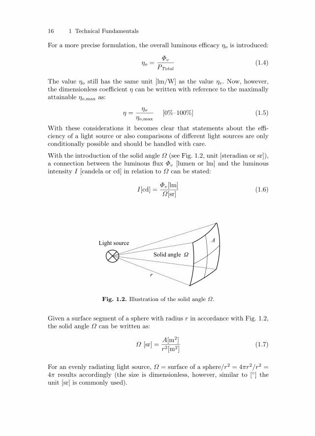
With the introduction of the solid angle Ω (see Fig. 1.2, unit [steradian or sr]),a connection between the luminous flux Φv [lumen or lm] and the luminousintensity I [candela or cd] in relation to Ω can be stated:

I[cd] =Φv[lm]Ω[sr]

(1.6)

A

r

Light source

Solid angle Ω

Fig. 1.2. Illustration of the solid angle Ω.

Given a surface segment of a sphere with radius r in accordance with Fig. 1.2,the solid angle Ω can be written as:

Ω [sr] =A[m2]r2[m2]

(1.7)

For an evenly radiating light source, Ω = surface of a sphere/r2 = 4πr2/r2 =4π results accordingly (the size is dimensionless, however, similar to [] theunit [sr] is commonly used).

ii


ii

ii

1.2 Light 17

From Eq. (1.6) two further values can be derived with reference to a radiatingor illuminated planar surface. These are the light density L [cd/m2] and theillumination level Ev [lux or lx]:

L[cd/m2] =I[cd]

Aradiating[m2](1.8)

Ev[lx] =Φv[lm]

Ailluminated[m2](1.9)

The light density L is a measure of the perceived brightness. A light source ap-pears all the brighter, the smaller the surface is in comparison to the luminousintensity.2

With the value Ev now also the so-called light exposure H [lux second] can bewritten as the product of illumination level Ev and time:

H[lx · s] = Ev[lx] · t[s] (1.10)

Here is a brief summary of the most important basic rules:

• The entire visible radiation of a light source is described with the value φv

(luminous flux, [lumen]).

• The light radiation relating to a solid angle is described with the value I(luminous intensity, [candela]).

• The light radiation relating to a receiving surface is specified with the valueEv (illumination level, [lux]).

• The specifications of illuminants (luminous flux, luminous intensity, . . . )apply to the perception of the human eye. Accordingly, in image process-ing the spectral sensitivity function V (λ) of the sensor, deviating fromthe function of the eye must be considered and compared to the spectraldistribution of the illuminant.

Finally, the recently introduced unit ANSI lumen is to be mentioned. It refersto the measurement of the radiant flux for the evaluation of projectors orother illumination equipment and the distribution of the luminous flux overthe lit surface (the so-called Nine Point Measurement). With modern commer-cial projectors however, the distribution is so even that it can be calculatedapproximately with Φv ≈ Φv,ANSI.

2 Here it is assumed that the irradiation takes place perpendicularly. If this is notthe case, it must be calculated vectorially. The angle is then incorporated into theequation.

ii


ii

ii


1.2.2 Illuminati

A list of different light sources is shown in Table 1.1.

It is noticeable that light emitting diodes (LED) have many advantages. SinceLEDs have actually replaced many other light sources, this technology will beexplained in detail in this section (see also [Hornberg 06: Chapter 3; TIS 07:white papers]).

There are other positive characteristics of the LED technology in addition tothe advantages shown in this table:

• LEDs have a good long-term consistency regarding light output and spec-tral light distribution.

• Their smallness makes the grouping of several LEDs to modular designs orthe use of special illumination designs possible.

• As LEDs operate with a regulated current source, they do not require ahigh-voltage ignition electronics, unlike HSI lamps, for example. A com-paratively simple power supply unit is sufficient. In the simplest case, thisis a series resistor.

• LEDs only require small supply voltages of approximately 1.5 VDC–3.5VDC. Illumination modules from several LEDs are thus easily designedfor low voltages of 5, 12 or 24 VDC or AC.

• Monochromatic LEDs produce an approximately monochromatic light.Thus, the chromatic aberration of the optic does no longer have any ef-fect.

• For a short time, LEDs can be operated with a much higher current, thanthe indicated maximal current. If they are operated in pulse mode andsynchronized with the camera, the luminous intensity increases (for moredetails see [Hornberg 06: Chapter 3]).

• LEDs are also available in the ultraviolet and infrared range.

From the data sheet of a modern light emitting diode, the meaning of theparameters becomes clear (Table 1.2).

Besides the advantages mentioned, LEDs also have some downsides: The lu-minous intensity of available LEDs is still not as high as those from traditionalilluminants such as halogen lamps or gas discharge lamps (for comparison: astandard data projector with HTI lamp: approximately 2 000 ANSI lumens,LED projector: 28 ANSI lumens – this is not a misprint).

When trying to emulate a very bright light source by the combination of multi-ple LEDs, the technical designer often fails because of the missing convection;with a too high component density the lost heat can no longer be dissipated.Also, the advantages of a very small illuminant with regard to an optimaldesign of the optics is then lost.

ii


ii

ii

1.2 Light 19

Cha

ract

eris

tics

Lig

ht s

ourc

e

Size

C

ost,

rela

ting

to

Φv

Effic

acy η,

ap

prox

. M

axim

um

lum

inou

s flux

Suit

abili

ty

for

diffus

e ill

umin

atio

n

Suit

abili

ty

for

dire

cted

ill

umin

atio

n

Suit

abili

ty

for

usag

e w

ith

lens

es

Usa

ge a

s st

robe

,

wit

h sy

nc

Agi

ng

effe

cts

Ope

rati

ng

hour

s ap

prox

..

Com

men

ts

Spir

al-w

ound

fila

men

t

0

+

+

1.

9—2.

6 %

−

−

−

0

−

−

1

000

Hal

ogen

+

+

2.

3—5.

1 %

+

−

0

+

−

−

3

000

Gre

at h

eat

gene

rati

on,

ther

efor

e fr

eque

ntly

use

d w

ith

fibe

r op

tics

. G

as d

isch

arge

(H

TI, H

SI ...)

+

−

15

—27

%

+

+

−

0

+

+

−

6

000

Gre

at h

eat

gene

rati

on,

ther

efor

e fr

eque

ntly

use

d w

ith

fibe

r op

tics

. N

eon,

lum

ines

cent

m

ater

ial

−

+

6.

6—15

%

+

+

+

− −

− −

−

+

7

500

Alm

ost

sole

ly u

sed

wit

h hi

gh

freq

uenc

y P

SU.

Lig

ht e

mit

ting

di

ode

+

+

0

5—

20 %

−

0

+

+

+

+

+

+

+

+

50

000

Diffe

rent

col

ors,

al

so a

vaila

ble

as

IR a

nd U

V, sm

all

size

(→

arr

ay

conf

igur

atio

ns).

Las

er d

iode

+

−

7—

12 %

−

− −

+

+

+

+

+

+

0

10

000

Usa

ge a

s “s

truc

ture

d lig

ht“.

Day

light

+

+

+

+

n/

a

±

Wea

ther

? D

ayti

me?

+

+

0 w

ith

lens

+

w

ith

mec

hani

cal

shut

ter

n/

a

+

+

Table 1.1. A comparison of different light sources. Efficiency η in accordance withEq. (1.5), data source for η: [Wikipedia 07, Luminous Efficacy].

ii


ii

ii

Excerpt – chapter truncated . . .

ii


ii

ii

2

Introduction to the Algorithmics

Author: Pedram Azad

2.1 Introduction

After having explained fundamentals of image acquisition from a technical per-spective in the previous chapter, now it will be explained how images can beprocessed with a computer. First of all, the mathematical model for the map-ping of an observed scene onto the image sensor is introduced. Subsequently,conventional encodings for the representation of images are explained, in orderto present a selection of image processing algorithms based upon these. Themodels and methods from this chapter serve as basis for the understandingof the implementation details and the numerous applications in the followingchapters of this book.

2.2 Camera Model and Camera Calibration

If metric measurements are to be accomplished with the aid of images, in twodimensions (2D) as well as in three dimensions (3D), then the understandingand the modeling of the mapping of a scene point on the image sensor arenecessary. In contrast, if the information of interest is coded exclusively in theimage, like in the case of the recognition of bar codes, the understanding ofthe representation of images in memory is sufficient. In any case it can onlybe advantageous not to regard the procedure of the mapping of a scene on theimage sensor from a mathematical view as black box.

ii


ii

ii

68 2 Introduction to the Algorithmics

2.2.1 Pinhole Camera Model

The central perspective model lies at the heart of almost all mathematicalmodels of the camera mapping function. As a basis for the understanding ofthe mathematical relationships, the wide-spread pinhole camera model serves.It is assumed that all points of a scene are projected to the image plane B viaa straight ray through an infinitesimally small point: the projection center Z.With conventional optics the projection center is located in front of the imageplane i.e. between the scene and the image plane. For this reason, the recordedimage is always a horizontally and vertically mirrored image of the recordedscene (see Fig. 2.1).

Object plane

Image plane (a)

Projection center

Image plane (b)

Fig. 2.1. Classic pinhole camera model (a), Pinhole camera model in positive posi-tion (b).

This circumstance has, however, no serious effects; the image is simply turned180 degrees. With a digital camera, the correct image is transmitted by trans-ferring the pixels in the opposite order from the chip. In order to computa-tionally model the pinhole camera model, the second theorem on intersectinglines is used, leading to: (

uv

)=

f

z

(xy

)(2.1)

where u, v denote the image coordinates and x, y, z the coordinates of a scenepoint in the 3D coordinate system whose origin is the projection center. The

ii


ii

ii

2.2 Camera Model and Camera Calibration 69

parameter f is known as the camera constant; it denotes the distance from theprojection center to the image plane. In practice, usually the projection centeris assumed to be lying behind the image plane – as in Eq. (2.1) – wherebyjust the sign of the image coordinates u, v is changed. In this way, the cameraimage is modeled as a central perspective projection without mirroring. Thisis referred to as the pinhole camera model in positive position.

Object plane

Z, Projection center

Image plane

x y

u v f

z

Fig. 2.2. The central perspective in a pinhole camera model in positive position.

2.2.2 Extended Camera Model

The pinhole camera model describes the mathematical relationships of the cen-tral perspective projection to a sufficient measure. It is, however, missing someenhancements for practical application, which are presented in the following.Firstly, some terms must be introduced and coordinate systems defined.

Principal axis: The principal axis is the straight line that runs perpendicu-larly to the image plane and through the projection center.

Principal point: The principal point is the intersection of the principal axiswith the image plane, specified in image coordinates.

ii


ii

ii


Image coordinate system: The image coordinate system is a two-dimen-sional coordinate system. Its origin lies in the top left-hand corner of the image,the u-axis points to the right, the v-axis downward. The units are in pixels.

Camera coordinate system: The camera coordinate system is a three-di-mensional coordinate system. Its origin lies in the projection center Z, the x-and y-axes run parallel to the u- and v-axes of the image coordinate system.The z-axis points forward i.e. toward the scene. The units are in millimeters.

World coordinate system: The world coordinate system is a three-dimen-sional coordinate system. It is the basis coordinate system, and can lie any-where in the area arbitrarily. The units are in millimeters.

There is no uniform standard concerning the directions of the image coordinatesystem’s axes and therefore also concerning the camera coordinate system’sx- and y-axes. While most camera drivers presuppose the image coordinatesystem as defined in this book, for example with bitmaps the origin is locatedin the bottom left-hand corner of the image and the v-axis points upward. Inorder to avoid the arising incompatibilities, the image processing library IVT,which underlies this book, converts the images of all image sources in such amanner that the previously defined image coordinate system is valid.

The parameters that fully describe a camera model are called camera parame-ters. One distinguishes intrinsic and extrinsic camera parameters. The intrinsiccamera parameters are independent from the choice of the world coordinatesystem, and therefore remain constant if the hardware setup changes. The ex-trinsic camera parameters, however, model the transformation from the worldcoordinate system to the camera coordinate system, and must be redeterminedif the camera pose changes. Up to now, the only (intrinsic) camera parame-ter in the pinhole camera model has been the camera constant f . A worldcoordinate system has not yet been considered and therefore neither have ex-trinsic camera parameters. So far it has also been assumed that the principalpoint lies at the origin of the image coordinate system, the pixels are exactlysquare pixels, and an ideal lens has been assumed that reproduces the scenedistortion-free.

The more realistic camera model defined in the following rectifies these disad-vantages. First of all, the pixels are assumed not to be square, but rectangular.Since in the camera constant the conversion factor from [mm] to [pixels] is con-tained, the different height and width of a pixel can be modeled by defining thecamera constant f independently for the u- and v-direction. The denotationsused in the following are fx and fy, usually referred to as the focal length, theunits are in pixels. With the inclusion of the principal point C(cx, cy), the newmapping from camera coordinates xc, yc, zc to image coordinates u, v reads:(

uv

)=(

cx

cy

)+

1zc

(fx xc

fy yc

)(2.2)

ii


ii

ii


Commonly, this mapping is also formulated as a matrix multiplication withthe calibration matrix

K =

fx 0 cx

0 fy cy

0 0 1

using homogeneous coordinates (see Appendix B.1.7):u · zc

v · zc

zc

= K

xc

yc

zc

(2.3)

The inverse of this mapping is ambiguous; the possible points (xc, yc, zc) thatare mapped to the pixel (u, v) lie on a straight line through the projectioncenter. It can be formulated through the inverse calibration matrix

K−1 =

1fx

0 − cx

fx

0 1fy− cy

fy

0 0 1

and the equation: xc

yc

zc

= K−1

u zc

v zc

zc

(2.4)

Here the depth zc is the unknown variable; for each zc the coordinates xc, yc,defined in the camera coordinate system, of the point (xc, yc, zc) are calculatedwhich maps to the pixel (u, v). In line with the notation from Eq. (2.2), themapping defined by Eq. (2.4) can analogously be formulated as follows:xc

yc

zc

= zc

u−cx

fxv−cy

fy

1

(2.5)

Arbitrary twists and shifts between the camera coordinate system and theworld coordinate system are modeled by the extrinsic camera parameters. Theydefine a coordinate transformation from the world coordinate system to thecamera coordinate system, consisting of a rotation R and a translation t:

xc = R xw + t (2.6)

where xw := (x, y, z) defines the world coordinates and xc := (xc, yc, zc) thecamera coordinates of the same 3D point. The complete mapping from theworld coordinate system to the image coordinate system can finally be de-scribed in closed-form by the projection matrix

P = K(R | t)

ii


ii

ii


using homogeneous coordinates:

u · sv · ss

= P

xyz1

(2.7)

If the mapping from Eq. (2.6) is inverted, then:

xw = RT xc −RT t (2.8)

where RT defines the transposed matrix of R, where for rotations it appliesR−1 = RT . Thus the inverse of the complete mapping from Eq. (2.7), whichis ambiguous like the inverse mapping from Eq. (2.4), can be formulated by:

xyz

= P−1

u · sv · ss1

(2.9)

with the inverse projection matrix

P−1 = RT (K−1| − t)

2.2.3 Camera Calibration

The calibration of a camera means the determination of both the intrinsicparameters cx, cy, fx, fy and the extrinsic parameters R, t. Beyond that, pa-rameters which model nonlinear distortions of the lens such as, for example,radial or tangential lens distortions, also belong to the intrinsic parameters.The modeling of such lens distortions is dealt with in Section 2.2.4; in this sec-tion, however, a purely linear camera mapping is first calculated, i.e. withoutdistortion parameters. The starting point for the test field calibration is a setof point pairs pw,i, Pb,i with i ∈ 1, . . . , n, where Pw,i ∈ R3 describes pointsin the world coordinate system and Pb,i ∈ R2 their projection into the imagecoordinate system.

On the basis of n ≥ 6 point pairs, which span a non-planar area, it is possibleto compute the camera parameters with the Direct Linear Transformation(DLT) [AbdelAziz 71]. In practice, however, a lot more point pairs are used,in order to achieve a more accurate result. For this purpose, a dot pattern ora checkerboard pattern (see Fig. 2.3) is usually recorded in several positions,whereby the dimensions of the pattern are accurately known. The difficulty isto know the relative position of the individual presentations of the pattern toeach other. A possible solution to this problem is the use of rectangular glassplates with a known thickness in combination with a perpendicular stop (see

ii


ii

ii


Fig. 2.3. Examples of calibration patterns.

Fig. 2.4. Example of a three-dimensional calibration object.

Fig. 2.5). A further possibility is the use of a three-dimensional calibrationobject (see Fig. 2.4).

However, with such a calibration object, it is hardly possible to obtain acomparably large number of points, which can be measured in the cameraimage and matched. In [Zhang 99], a calibration method is presented whichcomputes the relative motion between arbitrary presentations of the calibra-tion pattern on the basis of point correspondences, and thus makes the use ofa complex hardware setup unnecessary. This method is implemented in theOpenCV [OpenCV08] and is also used in the IVT for camera calibration.

Let now n ≥ 6 point pairs Pw,i(xi, yi, zi), Pb,i(ui, vi), i ∈ 1, . . . , n be given.On the basis of Eq. (2.7), we want for each point pair Pw(x, y, z), Pb(u, v) toapply:

ii


ii

ii


Fig. 2.5. Use of glass plates at a perpendicular stop for the camera calibration of alaser scanner (see [Azad 03]).

u · sv · ss

=

L1 L2 L3 L4

L5 L6 L7 L8

L9 L10 L11 L12

xyz1

(2.10)

This equation can be reformulated by division to:

u =L1x + L2y + L3z + L4

L9x + L10y + L11z + L12

v =L5x + L6y + L7z + L8

L9x + L10y + L11z + L12(2.11)

Since homogeneous coordinates are used, each real-valued multiple r ·P definesthe same projection, which is why w.l.o.g.1 L12 = 1 can be set. Multiplica-tion with the denominator and conversion finally leads to the two followingequations:

u = L1x + L2y + L3z + L4 − L9ux− L10uy − L11uz

v = L5x + L6y + L7z + L8 − L9vx− L10vy − L11vz (2.12)

1 Without loss of generality.

ii


ii

ii


With the aid of Eq. (2.12) and by using all n point pairs, now the followingover-determined linear system of equations can be set up:

x1 y1 z1 1 0 0 0 0 −u1x1 −u1y1 −u1z1

0 0 0 0 x1 y1 z1 1 −v1x1 −v1y1 −v1z1

......

......

......

......

......

...xn yn zn 1 0 0 0 0 −unxn −unyn −unzn

0 0 0 0 xn yn zn 1 −vnxn −vnyn −vnzn

L1

L2

L3

L4

L5

L6

L7

L8

L9

L10

L11

=

u1

v1

...un

vn

(2.13)

or short

A · x = b

As is shown in Appendix B, the optimal solution x∗ of this over-determinedsystem of linear equations in the sense of the Euclidean norm can be de-termined with the method of least squares. For this purpose, the followingequation, which results from left-sided multiplication of AT , must be solved:

AT A · x∗ = AT b (2.14)

One possibility for solving this system of linear equations is the use of theMoore Penrose pseudoinverse (AT A)−1. This can be calculated, for example,using the Cholesky decomposition (see Appendix B.2.3), since AT A is a sym-metrical matrix. The solution x∗ is then calculated by:

x∗ = (AT A)−1AT b (2.15)

If the DLT parameters L1 . . . L11 are determined, then the appropriate pixelPb(u, v) can be calculated with the assistance of the Eqs. (2.11) for any worldpoint Pw(x, y, z). Conversely, for any pixel Pb, the set of world points Pw thatmap to this pixel can be calculated by solving the following under-determinedsystem of equations:

(L9u− L1 L10u− L2 L11u− L3

L9v − L5 L10v − L6 L11v − L7

)xyz

=(

L4 − uL8 − v

)(2.16)

ii


ii

ii


The solution of this system of equations is the straight line g of all possibleworld points Pw, and can be calculated by the following steps:

a := L9u− L1

b := L10u− L2

c := L11u− L3

d := L9v − L5

e := L10v − L6

f := L11v − L7

g := L4 − u

h := L8 − v (2.17)

Using the definitions from Eq. (2.17), it now follows from the under-determinedsystem of linear equations from Eq. (2.16) by elimination of x:

(bd− ae)y + (cd− af)z = dg − ah (2.18)

With the following definition:

r := bd− ae

s := cd− af

t := dg − ah (2.19)

the parameter notation of the straight line g finally reads:xyz

=

gr−btartr0

+ u

bs−crarsr1

(2.20)

As was shown with the Eqs. (2.12) and (2.20), with the direct assistance ofthe DLT parameters L1 . . . L11, the camera mapping functions from 3D to 2Dand in reverse can be calculated. In some applications it can be moreover ofinterest to know the intrinsic and extrinsic parameters of the camera explicitly.

In particular, the knowledge of the intrinsic parameters is necessary for themodeling and the compensation of lens distortions (see Section 2.2.4). Theintrinsic parameters cx, cy, fx, fy and the extrinsic parameters R, t can be de-termined on the basis of the DLT parameters L1 . . . L11 with the aid of thefollowing calculations.

ii


ii

ii


The calculations are essentially taken from [More 02], although a few modifi-cations had to be made in order to be consistent with the introduced cameramodel.

L :=√

L29 + L2

10 + L211

cx =L1L9 + L2L10 + L3L11

L2

cy =L5L9 + L6L10 + L7L11

L2

fx =

√L2

1 + L22 + L2

3

L2− c2

x

fy =

√L2

5 + L26 + L2

7

L2− c2

y (2.21)

r31 =L9

L

r32 =L10

L

r33 =L11

L

r11 =L1L − cxr31

fx

r12 =L2L − cxr32

fx

r13 =L3L − cxr33

fx

r21 =L5L − cyr31

fy

r22 =L6L − cyr32

fy

r23 =L7L − cyr33

fy

R =

r11 r12 r13

r21 r22 r23

r31 r32 r33

t = R

L1 L2 L3

L5 L6 L7

L9 L10 L11

−1L4

L8

1

(2.22)

ii


ii

ii


ii


ii

ii

6

Workpiece Gauging

Author: Tilo Gockel

6.1 Introduction

A typical application of industrial image processing is workpiece gauging. InAppendix C, a concrete example with a commercial image processing tool willbe presented. In this chapter some basics are initially discussed.

Frequently the gauging procedure is used in combination with a transmittedlight illumination, and an image situation arises as in Fig. C.3 and C.5. Beforebeginning the actual measurement, a workpiece for which the relevant dimen-sions are correct (a so-called golden template) is placed under the camera, andthe system is thereby calibrated. The calibration takes place in such a mannerthat a known dimension is measured and the result of the measurement in theunit [pixel] together with the target result in [mm] or [inch] is stored.

Typically the scaling factors for u and v are determined in two measurements.Then, on the basis of the template part, position and nominal value for one ormore relevant dimensions are determined and stored.

The gauging of parts from the production line then takes place. By means of afeed, the workpiece comes under the camera. It is usually only ensured that theparts lie flat, the precise position and orientation is not known.1 Accordingly,the rotated position of the object must be determined by means of an alignmentbefore the actual measurement can start. The alignment can take place as inAppendix C, on the basis of known object features (in this example: center

1 Here and in the following example it is assumed: Optics and structure as in thecase studies from Appendix C.

ii


ii

ii

190 6 Workpiece Gauging

of area of the circular cut-outs), but a more general calculation based on themoments of area of higher order can also be used [Burger 06: Chapter 11.4;Kilian 01], as is shown in the following sections.

After the determination of the rotated position of the object, relevant grayscaletransitions on the outline, i. e. edges, can be found and measured.

6.2 Algorithmics

6.2.1 Moments

In this implementation, alignment takes place via calculating the area momentsof the object region. The moments of a region R in a grayscale image aredefined as follows:

mpq =∑

(u,v)∈R

I(u, v) · upvq (6.1)

For a binary image of the form I(u, v) ∈ 0, 1 the equation is reduced to:

mpq =∑

(u,v)∈R

upvq (6.2)

For calculation, see also Algorithm 39 and [Burger 06].

Algorithm 39 CalculateMoments(I, p, q) → mpq

mpq := 0for all pixels (u, v) in I do

if I(u, v) 6= 0 thenmpq := mpq + up · vq

end ifend for

The meaning of the zeroth and first order moments is particularly graphic.From them, the surface area and the center of area of a binary region can bedetermined as follows:

A(R) =∑

(u,v)∈R

1 =∑

(u,v)∈R

u0v0 = m00 (6.3)

ii


ii

ii

6.2 Algorithmics 191

u =1

A(R)·∑

(u,v)∈R

u1v0 =m10

m00(6.4)

v =1

A(R)·∑

(u,v)∈R

u0v1 =m01

m00(6.5)

Herein A(R) is the surface area and u, v are the coordinates of the center ofarea of the binary region R. With the introduction of these coordinates of theregion, it is now also possible to formulate the central moments. For this, theorigin of the coordinate system is shifted into the center of area, yielding:

µpq(R) =∑

(u,v)∈R

I(u, v) · (u− u)p · (v − v)q (6.6)

or for the special case of a binary region:

µpq(R) =∑

(u,v)∈R

(u− u)p · (v − v)q (6.7)

For the rotational alignment in this application, further calculation of the re-gion’s orientation is necessary. The angle θ between the major axis or principalaxis2 and the u axis is given by:

θ(R) =12

arctan(

2 · µ11(R)µ20(R)− µ02(R)

)(6.8)

The major axis has a direct physical basis just like the center of area: It isthe axis of rotation through the center of area, with which, when rotated, thesmallest moment of inertia arises. It should be noted that, with this equation,the orientation of the major axis can only be determined within [0, 180o).Section 6.3 shows an approach to determine the angle within [0, 360o).

With these moments a rotational alignment can now be performed for thegauging application in this chapter. For a further calculation regarding nor-malized central moments and invariant moments (for example, the so-called“Hu’s moments”), see [Burger 06: Chapter 11.4] and [Kilian 01].

Also, the moments for a binary region can be calculated much more efficientlyregarding only the contour of the region. For this approach, see [Jiang 91] and[OpenCV 07: Function cvContoursMoments()].

2 The associated axis is the minor axis. It lies orthogonal to the major axis and goesthrough the center of area.

ii


ii

ii


6.2.2 Gauging

The subpixel-precise determination of the grayscale transitions, i. e. edges,would have gone beyond the scope of the implementation in Section 6.4, butthe calculation for this is relatively straightforward and will briefly be intro-duced for the reader’s own implementations:

After alignment, a vertical edge of known height is to be measured. For this,the image row I(u, v = vc = const) is convolved with a one-dimensional edgefilter, for example in the form of (1, 0,−1). After comparison of the resultwith a given threshold value, the transition u0 is known with pixel-accuracy.3

A subpixel-precise determination can now take place via a parabolic fit withthe inclusion of two surrounding grayscale values on the line of the gradients.Given

I(u−1, vc) = i−1

I(u0, vc) = i0I(u+1, vc) = i+1

the subpixel-precise position of the grayscale transition in line vc can be cal-culated by:

uSubpixel = u0 +i−1 − i+1

2(i−1 − 2i0 + i+1)(6.9)

The calculation method results from the presumption of a Gauss-shaped distri-bution of the grayscale values in the gradient line. Furthermore, it is assumedthat the Gauss function near the maximum can be approximated by a parabola(for the derivation of this relation, see for example [Gockel 06: Chapter 3.2]).A prior smoothing of the grayscale values, for example with a Gauss filter, ishelpful. For further details see also [Hornberg 06: Chapter 8.7; Bailey 03; Bai-ley 05].

6.3 Implementation

In the program all available jpg files are loaded successively from the currentdirectory. For each file the following command steps are processed:

1. Conversion to grayscale, inversion4, binarization (here: using a fixedthreshold value of 128).

2. Moment calculation by means of the function cvMoments() from theOpenCV library.

3 The threshold value can be calculated for example on the basis of quantiles, seeSection 2.5.3.

4 The OpenCV function expects a white object on black background.

ii


ii

ii

6.3 Implementation 193

3. Calculation of the center of area of the region and determination of theangle θ of the major axis.

4. Determination of the orientation of the major axis using a function whichcounts the pixels belonging to the region along a straight line (this is amodified version of the function PrimitivesDrawer::DrawLine() fromthe IVT, here: WalkTheLine()). The line runs four times, in each casestarting from the center of area, along the major and minor axis, and thusspans an orthogonal cross with the crossing point in the center of area(see visualization). With the four results, the ambiguity of θ is resolved(compare the source code in Section 6.4).

5. Drawing the now determined coordinate system in the color image.

6. Rotating the binary image by θ (function ImageProcessor::Rotate(),see also Section 2.9).

7. Gauging of an (arbitrarily) specified dimension near the center of area,parallel to the minor axis. For this the function WalkTheLine() is usedagain.

8. Output of the image data and of the measured dimension in two windows(see Fig. 6.1).

Fig. 6.1. Screenshots from the implementation. Above: Stamping part with indicatedobject coordinate system. Below: Part after rotational alignment. Also indicated isthe cross used for the determination of θ and the measured cross-section line.

Notes: In the sample application, the scaling factors were not explicitly deter-mined, as it is the same procedure as the gauging of the workpiece. Moreover,to calculate the rotational alignment, in professional applications not the rota-

ii


ii

ii


tion of the entire image is implemented, but, more efficiently, only the rotationof the small probe area (see Appendix C).

As shown, the algorithms for moment calculation are also applicable tograyscale images, but the mentioned contour-based calculation can naturallyonly be applied to binary images.

Finally, it should be noted that in the literature, resolving the ambiguity of theorientation of the principal axis is recommended via computation of the cen-tralized moments of higher order (typically: observation of the change of signfrom µ30, see for example [Palaniappan 00]). From our experience, however, norobust decision is possible using this approach.

ii


ii

ii

6.4 References and Source Code 195

6.4 References and Source Code

[Bailey 03] D.G. Bailey, “Sub-pixel estimation of local extrema”, in: Proc. ofImage and Vision Computing, pp. 414–419, Palmerston North, New Zealand,2003. Available online:http://sprg.massey.ac.nz/publications.html

[Bailey 05] D.G. Bailey, “Sub-pixel Profiling”, in: 5th Int. Conf. on Information,Communications and Signal Processing, Bangkok, Thailand, pp. 1311–1315,December 2005. Available online:http://sprg.massey.ac.nz/publications.html

[Burger 06] W. Burger, M.J. Burge, “Digitale Bildverarbeitung”, Springer-Verlag, Heidelberg, 2006.

[Gockel 06] T. Gockel, “Interaktive 3D-Modellerfassung”, Dissertation, Uni-versitat Karlsruhe (TH), FB Informatik, Lehrstuhl IAIM Prof. R. Dillmann,2006. Available online:http://opus.ubka.uni-karlsruhe.de/univerlag/volltexte/2006/153/

[Hornberg 06] A. Hornberg (Hrsg.), “Handbook of Machine Vision”, Wiley-VCH-Verlag, Weinheim, 2006.

[Jiang 91] X.Y. Jiang, H. Bunke, “Simple and fast computation of moments”,in Journal: Pattern Recognition Archive, Volume 24, Issue 8, pp. 801–806,August 1991. Available online:http://cvpr.uni-muenster.de/research/publications.html

[Kilian 01] J. Kilian, “Simple Image Analysis by Moments Version 0.2”,OpenCV Library Documentation. Technical Paper (free distribution), onlinepublished, 2001. Available online:http://serdis.dis.ulpgc.es/~itis-fia/FIA/doc/Moments/OpenCv/

[OpenCV 07] Open Computer Vision Library. Open software library for com-puter vision routines. Formerly company Intel.http://sourceforge.net/projects/opencvlibrary

[Palaniappan 00] Palaniappan, Raveendran, Omatu, “New Invariant Mo-ments for Non-uniformly scaled Images”, Pattern Analysis and Applications,Springer, 2000.

ii


ii

ii

// ***************************************************************************

//// Project:

Alignment and Gauging for industrial parts.

// Copyright:

Tilo Gockel (Author)

// Date:

February 25th 2007

// Filename:

main.cpp

// Author:

Tilo Gockel, Chair Prof. Dillmann (IAIM),

//

Institute for Computer Science and Engineering (ITEC/CSE),

//

University of Karlsruhe. All rights reserved.

//// ***************************************************************************

//// Description:

// Program searches *.jpg−Files in the current directory. Then:

// calculation of center of gravity and principal axis for alignment,

// Then gauging (measurement) of a given distance,

//

//

// Algorithms:

// Spatial moments, central moments,

// calculation of direction of major axis,

// gauging (counting pixels to next b/w change), in [Pixels].

//

//

// Comments:

// OS: Windows 2000 or XP; Compiler: MS Visual C++ 6.0,

// Libs used: IVT, QT, OpenCV.

//

// ***************************************************************************

#include "

Imag

e/B

yteI

mag

e.h"

#include "

Imag

e/Im

ageA

cces

sCV

.h"

#include "

Imag

e/Im

ageP

roce

ssor

.h"

#include "

Imag

e/Im

ageP

roce

ssor

CV

.h"

#include "

Imag

e/Pr

imiti

vesD

raw

er.h"

#include "

Imag

e/Pr

imiti

vesD

raw

erC

V.h"

#include "

Imag

e/Ip

lIm

ageA

dapt

or.h"

#include "

Mat

h/C

onst

ants

.h"

#include "

Hel

pers

/hel

pers

.h"

#include "

gui/Q

TW

indo

w.h"

#include "

gui/Q

TA

pplic

atio

nHan

dler

.h"

#include <cv.h>

#include <qstring.h>

#include <qstringlist.h>

#include <qdir.h>

#include <iostream>

#include <iomanip>

#include <windows.h>

#include <string.h>

#include <math.h>

using namespace std;

// modified version of DrawLine(): returns sum of visited non−black pixels

Mon

tag

Feb

ruar

26,

200

7 23

:01

Sei

te 1

/6m

ain.c

pp

// (but here also used for line−drawing)

int WalkTheLine(CByteImage *pImage, const Vec2d &p1, const Vec2d &p2,

int r, int g, int b)

int pixelcount = 0;

const double dx = p1.x − p2.x;

const double dy = p1.y − p2.y;

if (fabs(dy) < fabs(dx))

const double slope = dy / dx;

const int max_x = int(p2.x + 0.5);

double y = p1.y + 0.5;

if (p1.x < p2.x)

for (int x = int(p1.x + 0.5); x <= max_x; x++, y += slope)

if (pImage−>pixels[int(y) * pImage−>width + x] != 0)

pixelcount++;

PrimitivesDrawer::DrawPoint(pImage, x, int(y), r, g, b);

else

for (int x = int(p1.x + 0.5); x >= max_x; x−−, y −= slope)

if (pImage−>pixels[int(y) * pImage−>width + x] != 0)

pixelcount++;

PrimitivesDrawer::DrawPoint(pImage, x, int(y), r, g, b);

else

const double slope = dx / dy;

const int step = (p1.y < p2.y) ? 1 : −1;

const int max_y = int(p2.y + 0.5);

double x = p1.x + 0.5;

if (p1.y < p2.y)

for (int y = int(p1.y + 0.5); y <= max_y; y++, x += slope)

if (pImage−>pixels[y * pImage−>width + int(x)] != 0)

pixelcount++;

PrimitivesDrawer::DrawPoint(pImage, int(x), y, r, g, b);

else

for (int y = int(p1.y + 0.5); y >= max_y; y−−, x −= slope)

if (pImage−>pixels[int(y) * pImage−>width + int(x)] != 0)

pixelcount++;

PrimitivesDrawer::DrawPoint(pImage, int(x), y, r, g, b);

return pixelcount;

Mon

tag

Feb

ruar

26,

200

7 23

:01

Sei

te 2

/6m

ain.c

pp


ii


ii

ii

void MomentCalculations(CByteImage *pImage, Vec2d &center,

PointPair2d &orientation, double &theta)

// calculate moments

IplImage *pIplInputImage = IplImageAdaptor::Adapt(pImage);

CvMoments moments;

cvMoments(pIplInputImage, &moments, 1); //1: treat grayvalues != 0 as 1

cvReleaseImageHeader(&pIplInputImage);

// for center of gravity

const double m00 = cvGetSpatialMoment(&moments, 0, 0);



// for angle of major axis

const double u11 = cvGetCentralMoment(&moments, 1, 1);



theta = 0.0;

// now: case differentiation:

// cmp.: [Johannes Kilian 01], Simple Image Analysis by Moments]

// online: http://serdis.dis.ulpgc.es/~itis−fia/FIA/doc/Moments/OpenCv/

// but: STILL AMBIGUOUS in n * 180 Degrees !

if ( ((u20 − u02) == 0) && (u11 == 0) )

// 1

theta = 0.0;

if ( ((u20 − u02) == 0) && (u11 > 0) )

// 2

theta = PI / 4.0;

if ( ((u20 − u02) == 0) && (u11 < 0) )

// 3

theta = − (PI / 4.0);

if ( ((u20 − u02) > 0) && (u11 == 0) )

// 4

theta = 0.0;

if ( ((u20 − u02) < 0) && (u11 == 0) )

// 5

theta = − (PI /2);

if ( ((u20 − u02) > 0) && (u11 > 0) )

// 6

theta = 0.5 * atan(2 * u11 / (u20 − u02));

if ( ((u20 − u02) > 0) && (u11 < 0) )

// 7

theta = 0.5 * atan(2 * u11 / (u20 − u02));

if ( ((u20 − u02) < 0) && (u11 > 0) )

// 8

theta = (0.5 * atan(2 * u11 / (u20 − u02))) + PI / 2;

if ( ((u20 − u02) < 0) && (u11 < 0) )

// 9

theta = (0.5 * atan(2 * u11 / (u20 − u02))) − PI / 2;

Math2d::SetVec(center, m10 / m00, m01 / m00);

// now: determine direction of major axis

// go cross−like, start from COG, go to borders

// count pixels... (cmp. visualization)

Vec2d v;

v.x = cos(theta) * 250 + center.x;

v.y = sin(theta) * 250 + center.y;

int count1 = WalkTheLine(pImage, center, v, 255, 0, 0);

v.x = cos(theta + PI) * 230 + center.x;

v.y = sin(theta + PI) * 230 + center.y;


Mon

tag

Feb

ruar

26,

200

7 23

:01

Sei

te 3

/6m

ain.c

pp

v.x = cos(theta + PI/2) * 230 + center.x;

v.y = sin(theta + PI/2) * 230 + center.y;


v.x = cos(theta − PI/2) * 230 + center.x;

v.y = sin(theta − PI/2) * 230 + center.y;


if ((count1 > count2) && (count3 < count4))

theta = theta + PI;

// Optional / for debugging: Console output

// cout << "Area: " << m00 << endl;

// cout << "Center (x,y): " << center.x << " " << center.y << endl;

// cout << "Theta [DEG]: " << ((theta * 180.0) / PI) << endl << endl;

int main(int argc, char *argv[])

double theta = 0.0;

QString path = QDir::currentDirPath();

QDir dir(path);

QStringList files = dir.entryList("

*.jp

g", QDir::Files);

if (files.empty())

cout << "

Err

or: c

ould

not

fin

d an

y *.

jpg

File

s" << endl;

return 1;

QStringList::Iterator it = files.begin();

QString buf = QFileInfo(path, *it).baseName();

buf += "

.jpg";

CQTApplicationHandler qtApplicationHandler(argc, argv);

qtApplicationHandler.Reset();

// width, height must be multiples of 4 (!)

CByteImage colorimage;

if (!ImageAccessCV::LoadFromFile(&colorimage, buf.ascii()))

printf("

erro

r: c

ould

not

ope

n in

put i

mag

e fi

le\n");

return 1;

CByteImage grayimage(colorimage.width, colorimage.height,

CByteImage::eGrayScale);

CByteImage binaryimage(colorimage.width, colorimage.height,

CByteImage::eGrayScale);

ImageProcessor::ConvertImage(&colorimage, &grayimage);

// calculations in grayimage and binaryimage

// drawings and writings in colorimage for display

CQTWindow imgwindow1(colorimage.width, colorimage.height);

imgwindow1.DrawImage(&colorimage);

Mon

tag

Feb

ruar

26,

200

7 23

:01

Sei

te 4

/6m

ain.c

pp


ii


ii

ii

imgwindow1.Show();

CQTWindow imgwindow2(binaryimage.width, binaryimage.height);

imgwindow2.DrawImage(&binaryimage);

imgwindow2.Show();

// main loop: cyclic loading all *.jpg in the directory and processing

while (!qtApplicationHandler.ProcessEventsAndGetExit())

buf = QFileInfo(path, *it).baseName();

buf += "

.jpg";

cout << buf.ascii() << endl;

if (!ImageAccessCV::LoadFromFile(&colorimage, buf.ascii()))

printf("

erro

r: c

ould

not

ope

n in

put i

mag

e fi

le\n");

return 1;

// Inversion: OpenCV calculates Moments for _white_ objects!

ImageProcessor::ConvertImage(&colorimage, &grayimage);

ImageProcessor::Invert(&grayimage, &grayimage); // (!)

ImageProcessor::ThresholdBinarize(&grayimage, &binaryimage, 128);

// Moments...

Vec2d center;

PointPair2d orientation;

MomentCalculations(&binaryimage, center, orientation, theta);

// Visualization / Output:

// Center

PrimitivesDrawerCV::DrawCircle(&colorimage, center, 3, 0, 255, 0, −1);

// Two Lines to show coordinate system

Vec2d v1, v2;

v1.x = cos(theta) * 100 + center.x;

v1.y = sin(theta) * 100 + center.y;

WalkTheLine(&colorimage, center, v1, 255, 0, 0);

v1.x = cos(theta + PI/2) * 100 + center.x;

v1.y = sin(theta + PI/2) * 100 + center.y;

WalkTheLine(&colorimage, center, v1, 255, 255, 0);

ImageProcessor::Rotate(&binaryimage, &binaryimage, center.x, center.y,

theta, true);

// we gauge the cross section near the minor axis

// (going parallel to the minor axis):

v1.x = center.x+5;

v1.y = center.y − 200;

v2.x = center.x+5;

v2.y = center.y + 200;

int i = WalkTheLine(&binaryimage, v1, v2, 255, 255, 255);

cout << "

Gau

ging

aft

er a

lignm

ent [

pixe

l]: " << i << endl << endl;

Mon

tag

Feb

ruar

26,

200

7 23

:01

Sei

te 5

/6m

ain.c

pp

char text[512];

sprintf(text, "

Cro

ss s

ectio

n in

pix

els:

%d", i);

PrimitivesDrawerCV::PutText(&colorimage, text, 20, 60, 0.8, 0.8,

255, 0, 100, 1);

imgwindow1.DrawImage(&colorimage);

imgwindow2.DrawImage(&binaryimage);

//Sleep(1200); // oops, too fast to see anything....

++it;

if (it == files.end()) it = files.begin(); // until hell freezes over

return 0;

Mon

tag

Feb

ruar

26,

200

7 23

:01

Sei

te 6

/6m

ain.c

pp


ii


ii

ii

11

Depth Image Acquisition with a Stereo CameraSystem

Author: Pedram Azad

11.1 Introduction

In Chapter 10, a 3D laser scanner was introduced, which is based on the light-section method. Since only the profile of an individual cross-section of theobject can be calculated on the basis of the projection of a laser line, onedegree of freedom between scan unit and object is necessary. In the presentedlaser scanner, this degree of freedom is realized by a mechanical rotation device,with the aid of which the scan unit can be rotated. All captured profiles formtogether a composite scan.

In this chapter, a procedure is now presented that is able to compute a scanwith a single image recording. A calibrated stereo camera system observes thescene to be captured, while a projector additionally structures the scene bythe projection of an random noise pattern. The calculation is again based ontriangulation, using the concepts for camera calibration, epipolar geometryand correlation, as described in Chapter 2. In comparison to the laser scan-ner, the same robustness cannot be achieved here, since the correlation-basedcorrespondence computation is more error-prone compared to the localizationof the laser line.

11.2 Procedure

The hardware setup of the system is shown in Fig. 11.1. As can be seen, a stereocamera system observes the scene, which is structured by the (uncalibrated)projector; the camera images of the two cameras are shown in Fig. 11.2.

ii


ii

ii

252 11 Depth Image Acquisition with a Stereo Camera System

Fig. 11.1. Left: System structure. Right: Calculated depth map for the image pairfrom Fig. 11.2. The points of the grid were enlarged by ∆×∆ = 4× 4 to achieve aclosed depth map.

Fig. 11.2. Example of an image pair as input to the stereo camera system. Left:Left camera image. Right: Right camera image.

First the stereo camera system must be calibrated. This is done using theapplication IVT/examples/CalibrationApp (see Chapter 10). The only dif-ference to the calibration of an individual camera is that the checkerboardpattern must be visible in both camera images at the same time.

The task of the algorithm is now to compute correspondences in the rightcamera image for image points in the left camera image. This takes placeby utilizing the epipolar geometry described in Section 2.10.2 and the ZeroMean Normalized Cross Correlation (ZNCC), as presented in Section 2.11.3.For each pixel in the left camera image, a (2k + 1) × (2k + 1) patch is cutout. This is normalized afterwards with respect to additive and multiplicativebrightness differences (see Section 2.11.3). Correspondences to this image patchare searched for along the epipolar line by calculating the ZNCC for each pointof the line. The pixel with the maximum correlation value then identifies the

ii


ii

ii

11.2 Procedure 253

correspondence. For the results in the Fig. 11.1 and 11.3, k = 10, i.e. a 21×21window, was used.

In order to make the approach more efficient and more robust, correspondencesare searched for only in a given interval dmin, . . . , dmax of so-called dispari-ties. The term disparity denotes the Euclidean distance from one point on theepipolar line to a given point in the other camera image. A small disparityrepresents a large distance to the camera, a large value a small distance. Fur-thermore, it should be noted that correspondences in the right camera imagemust lie in left direction, relative to the query point, on the epipolar line.

Since, as a result of occlusions, a (correct) correspondence cannot be deter-mined for every pixel, the candidates calculated by the correlation methodmust be validated on the basis of a threshold t. If the value computed by theZNCC is greater than this threshold, then the correspondence is accepted. Inthe presented system, t = 0.4 was selected.

An important measure for increasing the robustness is the recognition of ho-mogeneous image areas. Within such areas, correspondences cannot be deter-mined reliably, since good correlation results are calculated for a multiplicity ofdisparities; the best correlation result is determined by chance. The recognitionstep which is necessary for handling such cases, can be easily incorporated intothe normalization procedure of the image patch (see Section 2.11.3) aroundthe query point.

After having subtracted the mean value, the sum of the squared intensities∑∑I2(u, v) is a reliable measure for the homogeneity of the image patch: a

large value identifies a heterogeneous area, a small value a homogeneous area.In the presented system, image patches with values smaller than 100 · (2k+1)2

are rejected. After completion of the disparity calculation, the data is filteredby checking the existence of at least five neighbors with a similar disparity.

The disparity of each correspondence calculated in this way is finally enteredinto a so-called disparity map, in which bright pixels represent a small distancefrom the camera, and dark pixels a large distance (see Fig. 11.1). Additionally,for each correspondence (u1, v1), (u2, v2) the corresponding 3D point in theworld coordinate system is calculated using Algorithm 37 from Section 2.10.1.In order to obtain a higher accuracy, the computed integral disparities arerefined with sub-pixel precision using the procedure described in Section 6.2.2.

The result is finally a point cloud (see Fig. 11.3). If the point cloud is to betriangulated in order to obtain a 3D mesh, it is usually advantageous to choosethe points in the left camera image not at the full resolution, but in a gridwith a step size of ∆. In this system, ∆ = 5 was chosen. In this way, the noisecaused by the limited sub-pixel accuracy does not have a detrimental effect,and can be compensated by triangulation and smoothing. Furthermore, a stepsize of ∆ > 1 leads to a speedup by a factor of ∆2.

ii


ii

ii


The application functions as follows: Firstly, individual points in the left cam-era image can be set by a simple click with the left mouse button. The corre-lation result is visualized and displayed in the console. In this way, the min-imum and maximum disparity can be measured and adjusted with the slidecontrols. Now the area for which the depth information is to be calculated,can be selected by dragging a window with the mouse in the left camera im-age. After finishing the calculations, the application stores the disparity mapin the file depth_map.bmp, and the point cloud in xyz representation in thefile scan.txt. The point cloud can be triangulated and visualized using theapplication VisualizeApp (see Section 10.5.2).

Fig. 11.3. Result of a scan for the image pair from Fig. 11.2. Left: Point cloud.Right: Rendered mesh.

To conclude and as outlook it is to be mentioned that an optimized algorithmfor the correspondence computation can be used on rectified input images(see Section 2.10.3). This algorithm utilizes a recurrence in conjunction withrunning sum tables and thereby achieves a run-time that is independent of thewindow size. Optimized implementations for the generation of disparity mapsusing this algorithm achieve processing rates of 30 Hz and higher for inputimages of size 320×240. For a comprehensive overview, see [Faugeras 93].

11.3 References and Source Code

[Faugeras 93] O. Faugeras et al., “Real-time correlation-based stereo: algo-rithm, implementation and applications.”, INRIA Technical Report no. 2013,1993.

ii


ii

ii

// *****************************************************************************

// Filename: stereoscanner.cpp

// Copyright: Pedram Azad, Chair Prof. Dillmann (IAIM),

// Institute for Computer Science and Engineering (CSE),

// University of Karlsruhe. All rights reserved.

// Author: Pedram Azad

// Date: 2007/02/24

// *****************************************************************************

#include "

Imag

e/B

yteI

mag

e.h"

#include "

Imag

e/Im

ageP

roce

ssor

.h"

#include "

Imag

e/Pr

imiti

vesD

raw

er.h"

#include "

Mat

h/Fl

oatM

atri

x.h"

#include "

Cal

ibra

tion/

Ster

eoC

alib

ratio

n.h"

#include "

Vid

eoC

aptu

re/B

itmap

Cap

ture

.h"

#include "

gui/Q

TA

pplic

atio

nHan

dler

.h"

#include "

gui/Q

TW

indo

w.h"

#include "

Inte

rfac

es/W

indo

wE

vent

Inte

rfac

e.h"

#include <qslider.h>

#include <qlabel.h>

#include <qlcdnumber.h>

#include <math.h>

static CStereoCalibration *pStereoCalibration;

class CMessageReceiver : public CWindowEventInterface

public:

CMessageReceiver()

ok_point = false;

ok_rect = false;

void RectSelected(int x0, int y0, int x1, int y1)

ok_rect = true;

this−>x0 = x0; this−>y0 = y0;

this−>x1 = x1; this−>y1 = y1;

void PointClicked(int x, int y)

ok_point = true;

this−>x = x; this−>y = y;

int x, y;

bool ok_point;

int x0, y0, x1, y1;

bool ok_rect;

;Ja

n 16

, 08

2:08

Pag

e 1/

8st

ereo

scan

ner

.cpp

int SingleZNCC(const CByteImage *pInputImage1, CByteImage *pInputImage2,

int x, int y, int nWindowSize, int d1, int d2, float *values,

Vec2d &result, bool bDrawLine = false)

const int width = pInputImage1−>width;

const int height = pInputImage1−>height;

if (x < nWindowSize / 2 || x >= width − nWindowSize / 2 ||

y < nWindowSize / 2 || y >= height − nWindowSize / 2)

return −1;

const unsigned char *input_left = pInputImage1−>pixels;

unsigned char *input_right = pInputImage2−>pixels;

const int nVectorLength = nWindowSize * nWindowSize;

float *vector1 = new float[nVectorLength];


const int offset = (y − nWindowSize / 2) * width + (x − nWindowSize / 2);

const int diff = width − nWindowSize;

Vec2d camera_point = x, y ;

int i, j, offset2, offset3;

// Calculate the mean value

float mean = 0;

for (i = 0, offset2 = offset, offset3 = 0; i < nWindowSize; i++,

offset2 += diff)

for (j = 0; j < nWindowSize; j++, offset2++, offset3++)

vector1[offset3] = input_left[offset2];

mean += vector1[offset3];

mean /= nVectorLength;

// Subtract the mean value and apply

// multiplicative normalization

float factor = 0;

for (i = 0; i < nVectorLength; i++)

vector1[i] −= mean;

factor += vector1[i] * vector1[i];

if (factor < nWindowSize * nWindowSize * 100)

return −1;

factor = 1 / sqrtf(factor);


vector1[i] *= factor;

float best_value = −9999999;

int d, best_d = 0;

const int max_d = d2 < x ? d2 : x;

double m, c;

pStereoCalibration−>CalculateEpipolarLineInRightImage(camera_point, m, c);

// Determine the correspondence

for (d = d1; d <= max_d; d++)

Jan

16, 0

8 2:

08P

age

2/8

ster

eosc

anner

.cpp


ii


ii

ii

const int yy = int(m * (x − d) + c + 0.5) − nWindowSize / 2;

if (yy < 0 || yy >= height)

continue;

const int offset_right = yy * width + (x − d − nWindowSize / 2);

const int offset_diff = offset_right − offset;

// Calculate the mean value

float mean = 0;

for (i = 0, offset2 = offset_right, offset3 = 0; i < nWindowSize; i++,

offset2 += diff)

for (j = 0; j < nWindowSize; j++, offset2++, offset3++)

vector2[offset3] = input_right[offset2];

mean += vector2[offset3];

mean /= nVectorLength;

// Subtract the mean value and apply

// multiplicative normalization

float factor = 0;


vector2[i] −= mean;

factor += vector2[i] * vector2[i];

factor = 1 / sqrtf(factor);


vector2[i] *= factor;

float value = 0;


value += vector1[i] * vector2[i];

// Save correlation result for subpixel calculation

values[d] = value;

// Determine the maximum correlation value

if (value > best_value)

best_value = value;

best_d = d;

// Visualization

if (bDrawLine)

for (d = d1; d <= max_d; d++)

input_right[int(m * (x − d) + c + 0.5) * width + (x − d)] = 255;

result.x = x − best_d;

result.y = m * (x − best_d) + c;

delete [] vector1;

delete [] vector2;

return best_d;

Jan

16, 0

8 2:

08P

age

3/8

ster

eosc

anner

.cpp

bool ZNCC(CByteImage *pLeftImage, CByteImage *pRightImage,

CFloatMatrix *pDisparityMap, int nWindowSize, int d1, int d2,

float threshold, int step, int x0, int y0, int x1, int y1)

unsigned char *input_left = pLeftImage−>pixels;

unsigned char *input_right = pRightImage−>pixels;

float *output = pDisparityMap−>data;

int i;

const int width = pLeftImage−>width;

const int height = pLeftImage−>height;

const int nPixels = width * height;

const int nVectorLength = nWindowSize * nWindowSize;

for (i = 0; i < nPixels; i++)

output[i] = 0;

if (x0 < nWindowSize / 2) x0 = nWindowSize / 2;

if (y0 < nWindowSize / 2) y0 = nWindowSize / 2;

if (x1 > width − nWindowSize / 2) x1 = width − nWindowSize / 2;

if (y1 > height − nWindowSize / 2) y1 = height − nWindowSize / 2;

float *values = new float[width];



for (i = y0; i < y1; i += step)

for (int j = x0; j < x1; j += step)

Vec2d result;

const int best_d = SingleZNCC(pLeftImage, pRightImage, j, i,

nWindowSize, d1, d2, values, result);

if (best_d != −1 && values[best_d] > threshold)

const double y0 = values[best_d − 1];

const double y1 = values[best_d];

const double y2 = values[best_d + 1];

const double xmin = (y0 − y2) / (2 * (y0 − 2 * y1 + y2));

output[(i + nWindowSize / 2) * width + j + nWindowSize / 2] =

best_d + xmin;

printf("

i = %

i\n", i);

delete [] vector1;

delete [] vector2;

delete [] values;

return true;

Jan

16, 0

8 2:

08P

age

4/8

ster

eosc

anner

.cpp


ii


ii

ii

void Filter(CFloatMatrix *pDisparityMap, int step)

CFloatMatrix result(pDisparityMap);

const int width = pDisparityMap−>columns;

const int height = pDisparityMap−>rows;

const int stepw = step * width;

const float *data = pDisparityMap−>data;

const float max = 5;

ImageProcessor::Zero(&result);

for (int y = 0; y < height; y++)

for (int x = 0; x < width; x++)

const int offset = y * width + x;

if (data[offset] != 0)

// Determine the number of similar neighbors

int n = 0;

n += fabs(data[offset] − data[offset − step]) < max;

n += fabs(data[offset] − data[offset + step]) < max;

n += fabs(data[offset] − data[offset − stepw − step]) < max;

n += fabs(data[offset] − data[offset − stepw]) < max;

n += fabs(data[offset] − data[offset − stepw + step]) < max;

n += fabs(data[offset] − data[offset + stepw − step]) < max;

n += fabs(data[offset] − data[offset + stepw]) < max;

n += fabs(data[offset] − data[offset + stepw + step]) < max;

if (n >= 5)

result.data[offset] = data[offset];

ImageProcessor::CopyMatrix(&result, pDisparityMap);

int main(int argc, char **args)

CBitmapCapture capture("

test

_lef

t.bm

p", "

test

_rig

ht.b

mp");

if (!capture.OpenCamera())

printf("

Err

or: C

ould

not

ope

n ca

mer

a.\n");

return 1;

const int width = capture.GetWidth();

const int height = capture.GetHeight();

const CByteImage::ImageType type = capture.GetType();

CStereoCalibration stereo_calibration;

if (!stereo_calibration.LoadCameraParameters("

cam

eras

.txt"))

printf("

Err

or: C

ould

not

load

file

with

cam

era

\pa

ram

eter

s.\n");

return 1;

Jan

16, 0

8 2:

08P

age

5/8

ster

eosc

anner

.cpp

pStereoCalibration = &stereo_calibration;

CByteImage *ppImages[] = new CByteImage(width, height, type),

new CByteImage(width, height, type) ;

CFloatMatrix disparity_map(width, height);

CByteImage depth_image(width, height, CByteImage::eGrayScale);

CByteImage image_left(&depth_image), image_right(&depth_image);

// Initialize Qt

CQTApplicationHandler qtApplicationHandler(argc, args);

qtApplicationHandler.Reset();

// Create window

CMessageReceiver receiver;

CQTWindow window(2 * width, height + 180, &receiver);

// LCD numbers

QLCDNumber *pLCD_WindowSize = new QLCDNumber(3, &window);

pLCD_WindowSize−>setFixedWidth(80);

pLCD_WindowSize−>setFixedHeight(40);

pLCD_WindowSize−>move(20, height + 20);

QLCDNumber *pLCD_MinDisparity = new QLCDNumber(3, &window);

pLCD_MinDisparity−>setFixedWidth(80);

pLCD_MinDisparity−>setFixedHeight(40);

pLCD_MinDisparity−>move(20, height + 70);

QLCDNumber *pLCD_MaxDisparity = new QLCDNumber(3, &window);

pLCD_MaxDisparity−>setFixedWidth(80);

pLCD_MaxDisparity−>setFixedHeight(40);

pLCD_MaxDisparity−>move(20, height + 120);

// Sliders

QSlider *pSliderWindowSize = new QSlider(1, 49, 2, 21,

Qt::Horizontal, &window);

pSliderWindowSize−>setFixedWidth(400);

pSliderWindowSize−>setFixedHeight(20);

pSliderWindowSize−>move(120, height + 30);

QSlider *pSliderMinDisparity = new QSlider(0, 500, 1, 150,


pSliderMinDisparity−>setFixedWidth(400);

pSliderMinDisparity−>setFixedHeight(20);

pSliderMinDisparity−>move(120, height + 80);

QSlider *pSliderMaxDisparity = new QSlider(0, 500, 1, 220,


pSliderMaxDisparity−>setFixedWidth(400);

pSliderMaxDisparity−>setFixedHeight(20);

pSliderMaxDisparity−>move(120, height + 130);

// Labels

QLabel *pLabelWindowSize = new QLabel(&window);

pLabelWindowSize−>setText("

Win

dow

Siz

e");

pLabelWindowSize−>setFixedWidth(200);

pLabelWindowSize−>setFixedHeight(20);

pLabelWindowSize−>move(540, height + 30);

QLabel *pLabelMinDisparity = new QLabel(&window);

pLabelMinDisparity−>setText("

Min

imum

Dis

pari

ty");

pLabelMinDisparity−>setFixedWidth(200);

pLabelMinDisparity−>setFixedHeight(20);

Jan

16, 0

8 2:

08P

age

6/8

ster

eosc

anner

.cpp


ii


ii

ii

pLabelMinDisparity−>move(540, height + 80);

QLabel *pLabelMaxDisparity = new QLabel(&window);

pLabelMaxDisparity−>setText("

Max

imum

Dis

pari

ty");

pLabelMaxDisparity−>setFixedWidth(200);

pLabelMaxDisparity−>setFixedHeight(20);

pLabelMaxDisparity−>move(540, height + 130);

// Show window

window.Show();

while (!qtApplicationHandler.ProcessEventsAndGetExit())

const int nWindowSize = pSliderWindowSize−>value();

const int d1 = pSliderMinDisparity−>value();

const int d2 = pSliderMaxDisparity−>value();

pLCD_WindowSize−>display(nWindowSize);

pLCD_MinDisparity−>display(d1);

pLCD_MaxDisparity−>display(d2);

if (!capture.CaptureImage(ppImages))

break;

if (type == CByteImage::eGrayScale)

ImageProcessor::CopyImage(ppImages[0], &image_left);

ImageProcessor::CopyImage(ppImages[1], &image_right);

else

ImageProcessor::ConvertImage(ppImages[0], &image_left);

ImageProcessor::ConvertImage(ppImages[1], &image_right);

if (receiver.ok_rect)

ZNCC(&image_left, &image_right, &disparity_map, nWindowSize,

d1, d2, 0.4f, 4, receiver.x0,

receiver.y0, receiver.x1,

receiver.y1);

Filter(&disparity_map, 4);

// Calculate point cloud

FILE *f = fopen("

scan

.txt", "

w");

const float *disparity = disparity_map.data;

for (int y = 0, offset = 0; y < height; y++)

for (int x = 0; x < width; x++, offset++)

if (disparity[offset] != 0)

Vec3d world_point;

Vec2d point_left = x, y ;

double m, c;

stereo_calibration.CalculateEpipolarLineInRightImage(

point_left, m, c);

Vec2d point_right = x − disparity[offset],

m * (x − disparity[offset]) + c ;

stereo_calibration.Calculate3DPoint(point_left,

Jan

16, 0

8 2:

08P

age

7/8

ster

eosc

anner

.cpp

point_right, world_point, false);

fprintf(f, "

%f

%f

%f\

n", world_point.x, world_point.y,

world_point.z);

fclose(f);

// Calculate depth map

for (int i = 0; i < width * height; i++)

if (disparity_map.data[i] == 0)

disparity_map.data[i] = d1;

ImageProcessor::ConvertImage(&disparity_map, &depth_image);

depth_image.SaveToFile("

dept

h_m

ap.b

mp");

break;

if (receiver.ok_point)

Vec2d result;

float *values = new float[width];

const int best_d = SingleZNCC(&image_left, &image_right, receiver.x,

receiver.y, nWindowSize, 0, 400, values, result, true);

if (best_d != −1)

printf("

best

_d =

%i:

%f −−

%f −−

%f\

n", best_d,

values[best_d − 2], values[best_d], values[best_d + 2]);

delete [] values;

MyRegion region;

region.min_x = receiver.x − nWindowSize / 2;

region.max_x = receiver.x + nWindowSize / 2;

region.min_y = receiver.y − nWindowSize / 2;

region.max_y = receiver.y + nWindowSize / 2;

PrimitivesDrawer::DrawRegion(&image_left, region);

region.min_x = int(result.x + 0.5) − nWindowSize / 2;

region.max_x = int(result.x + 0.5) + nWindowSize / 2;

region.min_y = int(result.y + 0.5) − nWindowSize / 2;

region.max_y = int(result.y + 0.5) + nWindowSize / 2;

PrimitivesDrawer::DrawRegion(&image_right, region);

window.DrawImage(&image_left);

window.DrawImage(&image_right, width, 0);

delete ppImages[0];

delete ppImages[1];

return 0;

Jan

16, 0

8 2:

08P

age

8/8

ster

eosc

anner

.cpp


ii


ii

ii


book excerpt english

Documents