bond funds and fixed-income market liquidity: a stress-testing approach · penalized with outflows....
TRANSCRIPT

Technical Report No. 115 / Rapport technique no 115
Bond Funds and Fixed-Income Market Liquidity: A Stress-Testing Approach
by Rohan Arora, Guillaume Bédard-Pagé, Guillaume Ouellet Leblanc and Ryan Shotlander

The views expressed in this report are solely those of the authors. No responsibility for them should be attributed to the Bank of Canada.
ISSN 1919-689X © 2019 Bank of Canada
April 2019
Last updated on August 16, 2019
Bond Funds and Fixed-Income Market Liquidity: A Stress-Testing Approach
Rohan Arora, Guillaume Bédard-Pagé, Guillaume Ouellet Leblanc and Ryan Shotlander
Financial Markets Department Bank of Canada
Ottawa, Ontario, Canada K1A 0G9 [email protected]

i
Acknowledgements
For their valuable comments and suggestions, we thank Jason Allen, Ian Christensen and Virginie Traclet. We are also thankful to Adriano Palumbo for excellent research assistance. Finally, we thank Carole Hubbard and Jean-Sébastien Fontaine for editorial assistance.
ii
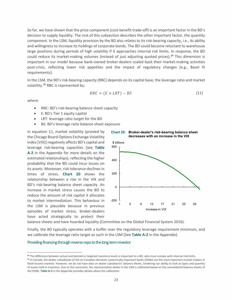
Abstract
This report provides a detailed technical description of a stress test model for investment funds called Ceto. The model quantifies how asset sales from investment funds could amplify a sudden decline in asset prices through the liquidity risk premium of the corporate bond market. Ceto is grounded in the literature on agents’ incentives and behaviour: it considers the response of investors to fund performance and the liquidity-management decisions of portfolio managers to meet demands for redemptions. The model also explicitly accounts for the provision of liquidity by broker-dealers and other potential buy-side investors. By accounting for the behaviour of different types of market participants, our approach allows us to account for the rich institutional features of, and heterogeneity within, the Canadian corporate bond market. The model can accommodate a range of different risk scenarios.
Bank topics: Economic models; Financial markets; Financial institutions; Financial stability JEL codes: G, G1, G2, G12, G14, G20, G23
Résumé
Ce rapport donne une description technique détaillée du modèle Ceto, utilisé pour soumettre les fonds de placement à des tests de résistance. À l’aide de la prime de risque de liquidité sur le marché des obligations de sociétés, le modèle permet de quantifier l’effet amplificateur possible de la vente d’actifs par les fonds de placement sur les prix d’actifs. Le modèle s’appuie sur les travaux traitant des motivations et du comportement des agents : il tient compte de la réaction des investisseurs au rendement des fonds ainsi que des décisions de gestion de la liquidité prises par les gestionnaires de portefeuille pour répondre aux demandes de rachat. Le modèle prend aussi explicitement en compte le rôle de fournisseurs de liquidité que jouent les courtiers en valeurs mobilières ou que pourraient jouer d’autres investisseurs. En intégrant le comportement de différents acteurs du marché, le modèle nous permet de tenir compte des spécificités et de l’hétérogénéité du marché des obligations de sociétés canadiennes. Le modèle peut se prêter à plusieurs scénarios de risques.
Sujets : Modèles économiques; Marchés financiers; Institutions financières; Stabilité financière Codes JEL : G, G1, G2, G12, G14, G20, G23

iii
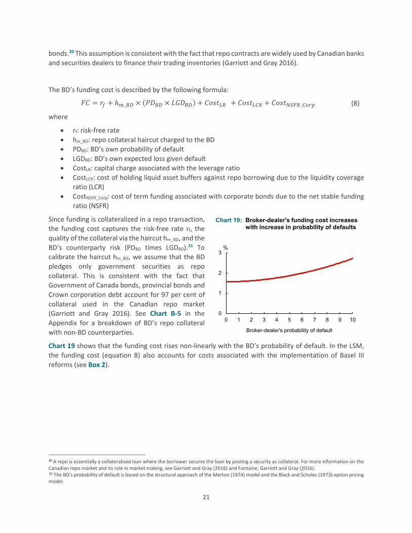
ContentsList of Tables ................................................................................................................................................................. iv
List of Figures ................................................................................................................................................................ iv
1 Introduction ........................................................................................................................................................... 1
2 Model topology and literature review ................................................................................................................... 2
3 Data: fund selection and stylized facts .................................................................................................................. 4
4 Stress-testing framework ...................................................................................................................................... 8
4.1 Liquidity demand module ............................................................................................................................ 9
Risk scenario ............................................................................................................................................ 9
Impact on fund net asset value.............................................................................................................. 10
Investor response to fund NAV .............................................................................................................. 11
Funds rebalance portfolios .................................................................................................................... 15
4.2 Liquidity supply module ............................................................................................................................. 16
Long-term investor ................................................................................................................................ 17
Broker-dealer ......................................................................................................................................... 19
Impact on market through the liquidity risk premium .......................................................................... 24
5 Model limitations................................................................................................................................................. 25
5.1 Data limitations .......................................................................................................................................... 25
5.2 Limitations—liquidity demand module ...................................................................................................... 26
5.3 Limitations—liquidity supply module ........................................................................................................ 26
5.4 Limitations—Ceto framework .................................................................................................................... 27
6 Conclusion ........................................................................................................................................................... 27
References ................................................................................................................................................................... 29
Appendix A................................................................................................................................................................... 33
Appendix B ................................................................................................................................................................... 38
Appendix C ................................................................................................................................................................... 39
Appendix D .................................................................................................................................................................. 40
Appendix E ................................................................................................................................................................... 42
iv
List of Tables Table 1: Details on an interest rate or credit spread shock in Ceto ............................................................................ 10 Table 2: Details on aggregate response choice set-ups in Ceto .................................................................................. 15
List of Figures Figure 1: Graphical representation of Ceto ................................................................................................................... 8 Figure 2: Main mechanisms of the liquidity demand module ....................................................................................... 9 Figure 3: Fund managers can adopt different strategies to meet investor redemptions ........................................... 16 Figure 4: Main mechanisms of the liquidity supply module ........................................................................................ 17 Figure 5: The price of immediacy depends on the reaction of liquidity supply and demand ..................................... 25

1
1 Introduction Risk-assessment models are an important component of the Bank of Canada’s analytical tool kit for assessing the resilience of the financial system (Christensen et al. 2015). They allow us to model financial channels that are important for financial stability and help us better understand how shocks could be transmitted and amplified within the financial system. For instance, the Framework for Risk Identification and Assessment (FRIDA) quantifies the impact of financial stability risks to households, businesses, banks and the broader economy. However, FRIDA does not capture propagation and amplification channels associated with non-bank market participants such as investment funds.1
This technical report presents Ceto, a stress-testing model that quantifies the impact of asset sales from investment funds on the Canadian corporate bond market via the liquidity risk premium. Figure 1 (see Section 4) provides a schematic overview of Ceto. Ceto is grounded in literature on agents’ incentives and behaviours: it considers the response of investors to fund performance and the liquidity-management decisions of portfolio managers in meeting redemptions. Also, the model explicitly accounts for provision of liquidity by broker-dealers and other buy-side investors. By modelling the behaviour of various market participants, Ceto accounts for the rich institutional features of, and the heterogeneity within, the Canadian corporate bond market. Ceto also expands sectoral coverage of our risk-assessment models beyond entities currently captured in FRIDA.
Like any model, Ceto faces uncertainty with regards to its parametrization and specification (Kozicki and Vardy 2017). It is particularly important to acknowledge this uncertainty when conducting financial stability risk assessments: models estimated using historical data containing a limited number of tail events might not adequately capture underlying economic mechanisms. In Ceto’s case, the model is estimated over a period when Canadian investment funds did not experience persistent outflows. Also, the willingness of broker-dealers to intermediate markets and of other buy-side investors to supply liquidity remains untested in times of stress. Consequently, expert judgment is required to calibrate the model and to capture structural changes in the financial system that can influence the materialization of risk scenarios and the generation of liquidity risk premium in Ceto.
Ceto follows in the footsteps of earlier initiatives at both international and national levels and adopts a recommendation from the Financial Stability Board (FSB): system-wide stress testing to capture the effects on financial system resiliency of collective selling by funds ( FSB 2017).2 Whether investment funds, through their management actions, constitute an important amplification channel for financial market shocks remains up for debate, but Ceto provides a coherent, systematic and tractable structure to study this question.
The rest of the report is organized as follows: Section 2 discusses the literature underpinning the mechanisms in Ceto and situates the model relative to its investment fund stress-testing peers; Section 3 provides stylized facts on Canadian fixed-income mutual funds—funds that are used to calibrate Ceto; Section 4 describes Ceto in detail and explains the modelling of mechanisms; Section 5 discusses model limitations; and Section 6 concludes.
1 For more details, see the Framework for Risk Identification and Assessment (FRIDA). 2 Central banks, international organizations and regulators are taking a closer look at investment funds to better understand macrofinancial implications of their growing role in credit intermediation. For example, please see European Central Bank (2017); Office of Financial Research (2016); and FSB (2017), subsection 2.4.4 Additional market liquidity considerations. For more details on global tends in non-bank financial intermediation, see the FSB (2019) Global Monitoring Report on Non-Bank Financial Intermediation 2018.

2
2 Model topology and literature review The model presented in this technical report is a stress-testing framework for Canadian fixed-income funds, more specifically fixed-income mutual funds with significant holdings of corporate bonds or other less-liquid assets.
Fixed-income funds are more vulnerable than other funds because they have a larger liquidity mismatch between their assets and liabilities: they offer daily redemption to investors, but invest in relatively less-liquid assets, such as corporate bonds. This liquidity mismatch raises concerns that they could face large redemption requests during periods of stress. If requested redemptions are larger than expected, fixed-income funds could collectively sell less-liquid assets and amplify volatility and illiquidity in the overall corporate bond market, raising potential financial stability concerns. This is because during periods of market stress, liquidity providers are less willing to supply liquidity and the cost of selling less-liquid assets increases (Dick-Nielsen, Feldhütter and Lando 2012; Nagel 2012). Therefore, we need tools such as stress-testing models to quantify the impact on the financial system when fixed-income funds, triggered by common redemption shocks, sell large quantities of assets.
A natural place to begin our review is to look at the broader literature on mutual funds. While the literature on equity mutual funds is large and dates to the 1980s, most academic work on fixed-income mutual funds and investment manager behaviour was undertaken only after the global financial crisis of 2008. Following the bankruptcy of Lehman Brothers in 2008, many money market mutual funds had to write down their holdings in Lehman’s securities, which led to large waves of redemptions by investors. For instance, Reserve Primary Fund saw more than 60 per cent of its assets under management withdrawn within two days as investors panicked after the fund’s net asset value (NAV) “broke the buck,” i.e., fell below a dollar (Anand, Gullapalli and Maxey 2008). This event was a watershed moment: it highlighted the challenges that could arise should such an event affect open-ended funds invested in less-liquid securities.
Investor flows into, and out of, mutual funds are largely determined by fund performance. Funds that outperform their benchmark return are rewarded with inflows, whereas those that underperform are penalized with outflows. Sirri and Tufano (1998) and Chevalier and Ellison (1997) analyze this flow-performance relationship for equity mutual funds and find that they face a convex flow-performance relationship, i.e., equity mutual funds that overperform experience large inflows, while underperforming funds do not see outflows at the same rate. In contrast, Goldstein, Jiang and Ng (2017) show that corporate bond mutual funds face a concave flow-performance relationship, i.e., underperforming corporate bond mutual funds experience outflows at an increasing rate (Chart E-1 in the Appendix). Arora (2018) corroborates this result for Canadian corporate bond mutual funds. The asymmetric relationship between flow and performance for corporate bond mutual funds is evidence of risk of redemption runs. Furthermore, this asymmetry varies with time and across fund characteristics: outflows due to underperformance are greater during episodes of market volatility and from funds with fewer holdings of liquid assets. The mechanisms and incentives for redemption runs in mutual funds are analogous to those in the bank run literature à la Diamond and Dybvig (1983).
Redemptions from fixed-income mutual funds, like other mutual funds, must be settled in cash. Fund managers can choose whether to draw on their liquid holdings or sell less-liquid assets such as corporate bonds to fulfill redemption requests. The decision to use liquid holdings to meet redemptions is described as horizontal slicing. Alternatively, the decision to sell assets proportionally to investment allocation is described as vertical slicing. Horizontal slicing reduces the liquidity of the fund portfolio in the subsequent period as liquid assets are used in the current period to meet redemption requests. In contrast, vertical

3
slicing maintains the liquidity of the fund portfolio in the subsequent period as assets are sold proportionally (see Arora and Ouellet Leblanc [2018] for more details on each strategy).
Liquidity-management decisions between horizontal and vertical slicing reflect an important trade-off: using liquid assets to meet redemptions reduces transaction costs and allows a fund to retain less-liquid assets, which carry higher expected returns, in its portfolio, but that comes at the cost of a greater liquidity mismatch between assets and liabilities. As previously discussed, a fund with a larger liquidity mismatch is more vulnerable to redemption runs. This is because there is a stronger first-mover advantage to investors to exit the fund en masse (i.e., a run on the fund) in the event of a negative shock (Chen, Goldstein and Jiang 2010; Diamond and Dybvig 1983).3
Funds’ approach to slicing remains highly debated, with empirical support for both horizontal and vertical slicing. Chernenko and Sunderam (2016) find that US equity funds tend to use horizontal slicing to meet redemptions, minimizing the impact of the sale of mutual fund on secondary markets. Jiang, Li and Wang (2017) corroborate this result for US corporate bond funds but find that firms switch liquidity management strategies, moving from horizontal slicing to vertical slicing, during periods of market stress. Arora and Ouellet Leblanc (2018) find a similar result for Canadian corporate bond mutual funds. The shift from horizontal to vertical slicing suggests that the trade-off changes under different market conditions. Redemption risk increases when volatility rises because there is a higher likelihood of negative fund returns. In this case, fund managers prefer vertical slicing to maintain the liquidity of their portfolios. Lastly, Morris, Shim and Shin (2017) show that bond fund managers can also engage in “cash hoarding,” whereby fund managers sell more assets than necessitated by redemptions to shore up liquidity for future periods.
Fund managers selling financial assets carries a price impact, a phenomenon that has been well studied in mutual fund literature. Coval and Stafford (2007) and Ben-Rephael, Kandel and Wohl (2012) show that sales and purchases of equity funds generate price pressure, which reverses over subsequent quarters. Likewise, Choi, Shachar and Shin (2018) show that transient price pressure caused by the flow of corporate bond funds exists in the US corporate bond market, and that these price pressures have substantial real effects by raising the cost of capital for firms during times of stress.
Having discussed the broader mutual fund literature relevant to investment fund stress-testing frameworks, we can now focus on exploring the stress-testing frameworks themselves. Cetorelli, Duarte and Eisenbach (2016) propose a linear model that quantifies the impact of an exogenous interest rate shock on outflows of corporate bond mutual funds. Their model analyzes spillover effects between corporate bond mutual funds, whereby sales from one fund depress market prices and in turn generate outflows and selling from other funds. Baranova, Liu and Shakir (2017) develop a liquidity supply model where the price discount is determined by the profit maximization of two representative agents (a broker-dealer and a leveraged investor), and Baranova et al. (2017) use this framework to stress test investment funds. Fricke and Fricke (2017) build a macroprudential stress-testing framework for investment funds based on the bank stress-testing model developed by Greenwood, Landier and Thesmar (2015). In the Fricke and Fricke model, leveraged institutional investors face a negative performance shock and are forced to deleverage by selling assets. These asset sales generate negative price pressure and affect mutual fund performances, triggering outflows from this sector, which further amplifies price declines.
3 In the context of redemption runs on bond funds, the first-mover advantage is that portfolio costs (liquidity discounts) incurred from selling less-liquid assets to meet redemptions are shouldered by investors who remain invested in the fund. Therefore, to avoid bearing these liquidation costs that are bought on by the redemption decisions of other investors, it is in an individual investor’s best interest to also withdraw from the fund, sparking a run. For a fuller treatment of this topic, please see Arora (2018).

4
Finally, Braun-Munzinger, Liu and Turrell (2016) construct an agent-based model of the corporate bond market with a variety of market participants, such as momentum traders, value traders, market makers, heterogenous investors and funds, to analyze the interactions between these agents and the associated impact on the underlying corporate bond market.
Our model quantifies the impact of sales of fixed-income mutual fund assets on the corporate bond liquidity premium using a liquidity demand module similar to Cetorelli, Duarte and Eisenbach (2016) and a liquidity supply function inspired by Baranova, Liu and Shakir (2017).
3 Data: fund selection and stylized facts In this section, we explain the selection of mutual funds and provide stylized facts regarding the sample.
The model uses Morningstar Direct as the primary data source for mutual fund allocations and fund characteristics. We also use Morningstar data on fund holdings together with Thompson Reuters fixed-income dataset as a supplementary data source to validate asset allocations. The sample period begins in January 2002 and ends in December 2018.
Selection criteria for funds are simple:
(i) The fund is an open-ended mutual fund domiciled in Canada. The fund is not a money-market fund, close-ended fund, fund of funds or exchange-traded fund.
(ii) The fund’s lifetime average assets under management (AUM) are greater than Can$50 million. (iii) The fund’s lifetime average investment in Canadian corporate debt is at least 20 per cent.
These criteria yield 324 funds, which we whittled down to 300 funds (full sample) based on the quality of the data and consistent reporting. We categorized the 300 funds by fund type into mixed and fixed-income funds, based on their lifetime average investment in equities. If a fund’s lifetime investment in equities was greater than or equal to 30 per cent, the fund was categorized as a mixed fund; otherwise, it was labelled as a fixed-income fund. The apportionment of funds between fixed-income and mixed is as follows: 67 funds were classified as mixed funds with all funds being actively managed; 233 funds were classified as fixed-income funds, of which 225 were actively managed; and the rest were index funds.4
The selection procedure captures mutual funds that are playing an increasingly important role in the Canadian corporate bond market. As seen in Chart 1, the sample’s post-crisis holdings of Canadian corporate debt accounted for 20 per cent of the outstanding Canadian-dollar-denominated corporate bond market in 2012, and approximately 23 per cent as of 2017. The magnitude of corporate bond assets held in these open-ended mutual funds gives us confidence in the fund selection procedure and gives Ceto a raison d’être.
4 The distinction between active and indexed funds is based on the index flag in Morningstar Direct.
0
10
20
30
2007 2009 2011 2013 2015 2017
%
Sources: Morningstar Holdings, Thomson Reuters, Statistics Canada and Bank of Canada calculations Last observation: December 2017
Monthly data
Post crisis, funds in the sample hold anincreasingly larger portion of the Canadian corporate bond market
Chart 1:

5
Over time, the fund sample experiences an increase not only in the assets managed by the mutual funds but also in the absolute number of funds. As shown in Chart 2, in the decade following the global financial crisis of 2008, the AUM of both fixed-income and mixed funds increased by nearly three times. Similarly, in Chart 3, the number of mutual funds grew by nearly 60 per cent for both fund types over the same time frame. Chart 2 and Chart 3 together point towards the idea that the increase in mutual fund holdings of Canadian corporate bonds is being driven by both inflows into pre-existing bond funds and increased inception of mutual funds with corporate fixed-income exposures.
Chart 4 highlights that on average for the mutual funds in our sample, the portion of portfolio allocated to corporate fixed-income securities rose from 36 per cent in 2007 to nearly 52 per cent in 2018. Also, for the same period, average allocations to more liquid asset classes, such as government securities, and cash and cash equivalents have declined. This indicates a greater mismatch between the liquidity profile of the investments held in the fund portfolio and the daily redemptions offered by open-ended mutual funds. In fact, the degree of liquidity mismatch becomes more apparent when we look at Chart 5, where we plot the liquidity profile of mutual funds in our sample across time. As seen in Chart 5, the average liquidity ratio of mutual funds in our sample, measured here as portfolio allocation to cash and cash equivalents, declined from 7 per cent in 2007 to close to 4 per cent in 2018.
30 48
117
195
0
60
120
180
240
2007 2012 2018
Number of funds
Mixed Fixed-income
The number of funds in our sample grew by 60 per cent from 2007 to 2018.
Last observation: 2018Q3
Chart 3:
Quarterly data
29
99 81
255
0
80
160
240
320
2007 2012 2018
AUM (billions)
Mixed Fixed-income
AUM for both fund types grew by nearly three times from 2007 to 2018
Sources: Morningstar Direct and Bank of Canada calculations
Chart 2:
Quarterly data
7 413 11
3625
3652
8 9
0
20
40
60
80
100
2007 2018
%
Cash and equivalents EquityGovernment bonds Corporate bondsOthers
Chart 4:
Sources: Morningstar Direct and Bank of Canada calculations
Fund allocation to corporate bonds has increased by 16 percentage pointsQuarterly data
Last observation: 2018Q3

6
Besides the increasing liquidity mismatch in the sample of mutual funds, we also find funds increasing their exposure to credit risk and duration. As shown in Chart 6, average fund allocations to high-yield assets increased from 10 per cent in 2007 to 17 per cent in 2018. Also, allocation to BBB-rated assets increased from 4 per cent in 2007 to 18 per cent in 2018—a trend that is consistent with other advanced economies (OECD 2019). The growth in allocation to high-yield and BBB-rated assets highlights a shift towards assets of lower credit quality. The increased credit risk in mutual fund portfolios could be explained by supply changes in the overall bond market. Nonetheless, it still represents increased system-wide exposure to credit risk (see Chart B-1 and Chart B-2 in the Appendix for more information on the credit quality of the broader Canadian bond market).
In the same vein, Chart 7 shows the cross-sectional distribution of duration for mixed and fixed-income funds in our sample over time. The average duration for fixed-income and mixed funds has increased slightly over time, with the average rising more quickly for fixed-income funds compared with their mixed counterparts. More interestingly, the distribution of duration has shifted upwards across time for both fund types, hinting that interest rate risk in the overall sample has also been on an uptrend. Again, like credit risk, the increase in interest rate risk could be driven by supply factors—corporations issuing more longer-dated debt in a low-interest rate environment—as opposed to fund managers actively deciding to increase their exposures (see Chart B-3 in the Appendix for more information on the duration of the broader Canadian bond market).
Therefore, mutual funds with large exposures to Canadian corporate bonds have increased in size and systemic importance. Moreover, these funds have experienced an uptick in their exposure to credit risk and interest rate risk, while lowering their holdings of liquid assets. Hence, these funds are vulnerable to
4322
43
43
4
18
10 17
2007 20180
20
40
60
80
100%
AAA AA to A BBB BB to below B
Since 2007, allocation to BBB-rated debt has increased by 14 percentage points
Sources: Morningstar Direct and Bank of Canada calculations
Chart 6:
Quarterly data
Last observation: 2018Q3
Investment grade High yield
2007 2008 2009 2010 2011 2012 2013 2014 2015 2016 2017 20180
2
4
6
8
10
12%
Liquidity ratio Worst quarterly outflow5th percentile quarterly outflow 10th percentile quarterly outflow
Chart 5:
Last observation: 2018Sources: Morningstar Direct and Bank of Canada calculations
Annual dataThe average liquidity ratio of funds has reached its lowest level since 2007

7
interest rate and credit shocks that could trigger large outflows. In the face of these outflows, funds might be obligated to sell less-liquid corporate bond assets in a short time frame, consequently testing the liquidity of the Canadian corporate bond market.
The liquidity demand module in Ceto estimates the outflows experienced in our sample for a given risk scenario. Since we use historical flow and return patterns for the sample mutual funds to calibrate expected flows at the fund level, we present the returns of our sample of mutual funds in Chart 8. The sample’s largest period of underperformance came during the 2008 financial crisis. Also, since fixed-income funds outnumber and outweigh mixed funds in the sample, the sample captures periods of bond market turbulence such as the taper tantrum in 2013 and Canada’s oil shock of 2015. Therefore, the fund sample captures a variety of market conditions, which strengthens the empirical foundations of Ceto.5
Chart 9 is a scatterplot of the flows of the full sample of 300 mutual funds and their historical returns at a quarterly frequency. As one can observe, there exists a distinct positive flow-return relationship. Moreover, the worst outflows experienced by the sample in one quarter are close to 3 per cent, while the largest inflows stand at approximately 5 per cent in one quarter.
5 In Chart 8 we present the fund sample’s performance only from 2007 onwards; however, for calibration purposes we use flow and return data from 2002 onwards, allowing for a longer time series.
-3
-2
-1
0
1
2
3
4
5
2007 2009 2011 2013 2015 2017
Returns (%)
Chart 8:
Sources: Morningstar Direct and Bank of Canada calculations Last observation: 2018Q3
The fund sample's largest period of underperformance was in 2008Quarterly data
2007 2012 2018 2007 2012 2018
Fixed-income Mixed
4
5
6
7
8Duration
Average
Chart 7:
Sources: Morningstar Direct and Bank of Canada calculations Last observation: 2018Q3Note: The bars represent the interquartile range.
Average duration and overall distribution of duration have been increasing for both fund typesQuarterly data
-3-2-1012345
-3 -2 -1 0 1 2 3 4 5
Flows (%)
Returns (%)
45⁰ (for reference)
Chart 9:
Sources: Morningstar Direct and Bank of Canada calculations Last observation: 2018Q3
As expected, there exists a positive flow-return relationship in our mutual fund sampleQuarterly data

8
Lastly, Chart 10 presents two empirically estimated probability distributions over the sample’s historical flows. The kernel distribution, which is non-parametric, when compared with the normal distribution, shows that historically flows have been non-Gaussian, with more mass in the tails, i.e., higher probability of large inflows and outflows as compared with a Gaussian distribution. Finally, the average of both distributions lies above 0 per cent, indicating that historically mutual funds in our samples are more likely to have experienced slight inflows, as opposed to outflows. These distributions help in contextualizing outflows, experienced by the sample in the face of our risk scenario, in terms of standard deviations from the historical mean.
4 Stress-testing framework As presented in Figure 1, Ceto is made up of two modules: a liquidity demand module and a liquidity supply module. The modules operate sequentially to quantify the impact of asset liquidations by bond funds on liquidity in the Canadian corporate bond market. Market liquidity here is measured by the liquidity risk premium, which reflects the compensation that bond funds must pay to access liquidity in the secondary bond market. The first block in Figure 1 (liquidity demand) is used as an input into the second block (liquidity supply). We abstract from any feedback or general equilibrium effects at this time to keep the model tractable, but potential improvements are discussed in the model limitations section of this report.
Figure 1: Graphical representation of Ceto
The model starts with an exogenous shock (i.e., a risk scenario) to market risk factors that affects the value of funds’ asset holdings. Since the focus is on bond funds, the shock would generally include changes in interest rates, but other factors such as changes in credit spreads are also considered.
The shock causes a decline in the net asset value (NAV) of funds’ holdings, reducing the performance of funds. The decline in performance causes investors to reassess their investments, leading some of them
0
5
10
15
20
25
-7.5 -5 -2.5 0 2.5 5 7.5
Probabilty (flows)
Flows (%)
Normal
Kernel
Chart 10:
Sources: Morningstar Direct and Bank of Canada calculations Last observation: December 2018
Fund outflows are non-Gaussian, with a skew towards inflows compared with outflowsMonthly data

9
to redeem their fund shares. Redemption requests by investors are settled in cash, forcing fund managers to rebalance their portfolios. This rebalancing generates sales of corporate bonds from bond funds. In the second module, we assess the compensation required by other market participants (broker-dealers and long-term investors) to absorb this demand for liquidity from bond funds. This compensation is proxied by the liquidity premium in the corporate bond market.
4.1 Liquidity demand module This section describes the liquidity demand module (LDM) of Ceto. The LDM quantifies the amount of corporate bonds sold (in dollars) by bond funds to meet their investors’ redemption requests. The LDM is based on the linear model for liquidity demand developed by Cetorelli, Duarte and Eisenbach (2016).
Figure 2 outlines the main mechanisms of the LDM. An exogenous risk scenario, given by change in interest rates or change in credit spreads, results in a decline in fund NAV through the portfolio duration metric. Investors observe the decline in fund NAV, and some of them respond by redeeming from the fund. The amount of redemptions experienced by a fund for a given decline in NAV is based on the fund’s flow-performance sensitivity, a metric calibrated from historical data for each fund. A fund’s flow-performance sensitivity is a function of fund characteristics, namely, fund size, a fund’s holdings of liquid assets, etc. The fund manager then rebalances portfolios to meet investors’ redemption requests. The liquidity strategy employed by the fund manager decides the amount of corporate bonds sold by the fund to meet redemption requests. Corporate bond sales across all funds are then summed together to determine the aggregate demand for liquidity for corporate bonds (Q). This is used as an input by the liquidity supply module.
The LDM section is structured as follows: the first subsection discusses the types of risk scenario that can be entered into Ceto, the second links risk scenario to portfolio duration, the third explains the fund-level flow-performance calibration in greater depth, and the last subsection describes liquidity management strategies.
Figure 2: Main mechanisms of the liquidity demand module
Risk scenario The first step in Ceto is to determine the risk scenario. This has three dimensions: (i) type of shock, (ii) magnitude of shock, and (iii) time period of shock. The type and magnitude of the shock are discussed in detail in Table 1. The time period of the shock is a specific quarter of a year. The quarterly time step means that the shock should be interpreted as a shock lasting the entire quarter. The time period of the shock pins down the sample of mutual funds subject to the risk scenario. The time-period dimension is critical because the number of funds, fund asset sizes, and fund asset allocations are time varying (recall Charts 2, 3 and 4). Therefore, Ceto allows us to analyze the impact of the same risk scenario over different periods.

10
Table 1: Details on an interest rate or credit spread shock in Ceto Shock type Interest rate shock Credit spread shock
Interpretation A parallel shift in the Government of Canada zero-coupon yield curve
A rise in Canadian credit spreads by credit quality
Magnitude Basis points per quarter Basis points per quarter per credit quality
Mathematical form
A constant
Example: [25] represents a parallel shift in the Government of Canada zero-coupon yield curve by 25 basis points in one quarter
A 7-by-1 vector with each entry corresponding to a credit rating. The vector elements are order dependant as each element corresponds to a credit rating:
[AAA, AA, A, BBB, BB, B, Below B].
Example: [25, 50, 75, 100, 125, 150, 175] reflects an increase in credit spreads for [AAA, AA, A, BBB, BB, B, Below B] in basis points in one quarter
Impact on fund net asset value Both the interest rate and the credit spread shock affect a fund’s NAV through the duration metric; however, the exact mechanism differs slightly.6
For the interest rate shock scenario, the impact on the fund’s NAV is obtained by multiplying the fund’s duration and the interest rate shock.
∆𝑁𝑁𝑁𝑁𝑉𝑉𝑖𝑖,𝑡𝑡 = ∆𝑟𝑟 × 𝑑𝑑𝑖𝑖,𝑡𝑡 (1)
where
• ∆𝑁𝑁𝑁𝑁𝑉𝑉𝑖𝑖,𝑡𝑡 : change in NAV of fund i at time t • ∆𝑟𝑟 : interest rate shock • 𝑑𝑑𝑖𝑖,𝑡𝑡 : duration of fund i at time t
For the credit shock, it is necessary first to calculate the weighted aggregate increase in credit spreads experienced by the fund’s portfolio. This is done by multiplying each element of the credit shock vector by the element of the weight vector, which represents the fund’s exposure to each level of credit quality at a point in time.
∆𝑟𝑟𝑤𝑤𝑖𝑖,𝑡𝑡 = ∆𝒓𝒓 × 𝒘𝒘𝑖𝑖,𝑡𝑡𝑇𝑇 𝑠𝑠. 𝑡𝑡. ∑ 𝑤𝑤𝑖𝑖,𝑡𝑡𝑖𝑖 = 1 (2)
where
6 Duration is the sensitivity of a fixed-income instrument to parallel shifts in the zero-coupon yield curve. For a mutual fund, fund-level duration is the weighted average duration of all fixed-income positions, where the weights are based on the market value of each position.

11
• ∆𝑟𝑟𝑤𝑤𝑖𝑖,𝑡𝑡 : weighted aggregate credit shock for fund i at time t • ∆𝒓𝒓 : credit spread shock vector • 𝒘𝒘𝑖𝑖,𝑡𝑡 : weight vector for fund i at time t • ∑ 𝑤𝑤𝑖𝑖,𝑡𝑡𝑖𝑖 = 1 : required condition that the sum of the elements of the weight vector is equal to one
The weighted aggregate credit shock is then multiplied by the fund’s duration to determine the impact on the fund’s NAV, as seen in equation 1.7
Investor response to fund NAV The decline in fund NAV is observed by fund investors, who respond by redeeming a part of their investment in the fund, thus generating outflows. It is necessary to estimate these outflows.
As described in Section 2, the literature shows that flows are driven by fund performance. A fund that performs well attracts investor capital (i.e., the fund experiences inflows), while a fund that performs poorly sees investors withdrawing capital (i.e., the fund experiences outflows).
Different measures of fund performance could be considered: return of the fund portfolio, excess return of the fund portfolio over a benchmark, a fund’s alpha based on the capital asset pricing model (CAPM), and a fund’s Sharpe ratio.8 In Ceto, we measure fund performance using a CAPM-based alpha because it allows us to control for market factors and pick variables that will impact fund performance. Our CAPM specification comes from Cetorelli, Duarte and Eisenbach (2016), where the empirically estimated fund level (𝜶𝜶𝒊𝒊,𝒕𝒕) captures fund performance being driven by the bond market factor and removes equity market effects. The controlled equity market factor and the uncontrolled bond market factor are necessary to align the risk scenario with expected outflows. In Ceto, we shock the bond market factor through the interest rate or credit channel. The fund-level alpha consists primarily of bond market effects, as we have removed equity market effects, allowing for better alignment between the risk scenario and its subsequent impact on fund performance.9
𝑅𝑅𝑖𝑖,𝜏𝜏 = 𝜶𝜶𝒊𝒊,𝒕𝒕 + 𝛽𝛽𝑖𝑖,𝑡𝑡�𝐸𝐸𝑅𝑅𝜏𝜏𝑒𝑒𝑒𝑒𝑒𝑒𝑖𝑖𝑡𝑡𝑒𝑒� + 𝜖𝜖𝑖𝑖,𝜏𝜏 ∀ 𝜏𝜏 = 𝑡𝑡 − 11, … , 𝑡𝑡 (3)
where
• 𝑅𝑅𝑖𝑖,𝜏𝜏 : the excess return of fund i at time 𝜏𝜏, where 𝜏𝜏 is one of the preceding 12 months • 𝛼𝛼𝑖𝑖,𝑡𝑡 : fund i’s alpha at time t estimated using its previous 12-month excess returns • 𝛽𝛽𝑖𝑖,𝑡𝑡 : fund i’s equity market beta at time t estimated using its 12-month excess returns
• 𝐸𝐸𝑅𝑅𝜏𝜏𝑒𝑒𝑒𝑒𝑒𝑒𝑖𝑖𝑡𝑡𝑒𝑒 : excess return of equity market at time 𝜏𝜏, where 𝜏𝜏 is one of the preceding 12 months
• 𝜖𝜖𝑖𝑖,𝜏𝜏 : CAPM model error term for fund i at time 𝜏𝜏, where 𝜏𝜏 is one of the preceding 12 months
7 We make the simplifying assumption here that duration does not depend on credit quality, which is not the case in practice. This is due to data limitations because Morningstar Direct does not break down fund-level duration by credit quality of holdings. To account for the impact of credit quality on duration, we would need to calculate fund-level duration from Morningstar holdings merged with credit-quality data. As these data become available to the Bank, we will adjust future versions of the stress-testing framework. 8 All these measures of performance have been used previously in mutual fund literature. Refer to Sharpe (1966), Grinblatt and Titman (1989), Grinblatt and Titman (1993), Elton, Gruber and Blake (1996) and Barras, Scaillet and Wermers (2010) as a few examples. 9 The equity market factor is the S&P 500 total market return, and the risk-free rate is the one-month US Treasury rate. The results are robust to the use of the SP/TSX composite index as the equity market factor and the one-month Canadian treasury bill rate as the risk-free rate.

12
The alpha is estimated over a 12-month rolling window to capture time-series variation in fund performance. This time series of estimated alpha is used, as an input, to determine the relationship between fund flows and fund performance.
𝐹𝐹𝐹𝐹𝐹𝐹𝑤𝑤𝑖𝑖,𝑡𝑡 = 𝛿𝛿𝑖𝑖 +𝜝𝜝𝒊𝒊�𝜶𝜶�𝒊𝒊,𝒕𝒕� + 𝜀𝜀𝑖𝑖,𝑡𝑡 (4)
where
• 𝐹𝐹𝐹𝐹𝐹𝐹𝑤𝑤𝑖𝑖,𝑡𝑡 : the flows experienced by fund i at time t, represented as a percentage of the preceding month’s AUM, i.e., at t-1
• 𝛿𝛿𝑖𝑖 : regression intercept for fund i • Β𝑖𝑖 : fund i's sensitivity to fund performance • 𝛼𝛼�𝑖𝑖,𝑡𝑡 : empirically estimated fund i’s alpha at time t obtained from equation 3 • 𝜀𝜀𝑖𝑖,𝑡𝑡 : regression error term for fund i at time t
The empirically estimated fund-level beta (𝜝𝜝𝒊𝒊) captures the sensitivity between fund performance and fund flows.10
Outflows from a fund for a given decline in fund NAV are estimated by a multiplication between the decline in NAV and the fund-level beta.
𝑂𝑂𝑂𝑂𝑡𝑡𝑂𝑂𝐹𝐹𝐹𝐹𝑤𝑤i,t = ∆𝑁𝑁𝑁𝑁𝑉𝑉𝑖𝑖,𝑡𝑡 × Βi (5)
where
• 𝑂𝑂𝑂𝑂𝑡𝑡𝑂𝑂𝐹𝐹𝐹𝐹𝑤𝑤𝑖𝑖,𝑡𝑡 : outflows from fund i at time t expressed as a percentage of fund AUM at time t • ∆𝑁𝑁𝑁𝑁𝑉𝑉𝑖𝑖,𝑡𝑡 : change in NAV of fund i at time t due to the shock scenario obtained from equation 1 • Β𝑖𝑖 : fund i’s sensitivity to fund performance obtained from equation 4
Beta is estimated once for each fund; therefore, any shifts in the cross-sectional estimates over time are driven by the entry and exit of funds from our sample (i.e., by the birth and demise of funds over time).
10 The fund-level beta estimated in our framework suffers from biases. As per the literature, the beta estimate is time-varying and increases during periods of market stress, as evidenced in Goldstein, Jiang and Ng (2017) and Arora (2018). In Ceto, we estimate a single beta for each fund, which does not change with time, because most funds do not have large enough histories to confidently estimate fund-level beta over different time periods. Therefore, the betas used in Ceto are a lower bound on potential outflows for the given decline in NAV during times of stress.

13
Chart 11 presents the cross-sectional average beta and the corresponding interquartile range, by fund type. It shows that:
(i) As expected, the average beta is higher for fixed-income funds than for mixed funds since the former are less liquid.
(ii) The distribution of beta has shifted upwards over time for both fixed-income and mixed funds, suggesting that fund outflows have become more sensitive to bond market performance over time. This is likely due to a variety of factors, including post-crisis entry of smaller funds, which tend to have a larger beta (Chart 13) and a higher number of funds with fewer liquid holdings (Chart 14 and Chart 15).
Chart 12 presents the average beta for each fund type across the entire sample. Again, the results are in line with expectations, as the average beta for fixed-income funds is higher than that of mixed funds. Furthermore, since the number and asset size of fixed-income funds are larger that those of mixed funds, the full sample average beta is closer to the fixed-income funds’ average.
4.323.90
4.45
0
1
2
3
4
5
Full sample Mixed Fixed-income
BetaChart 12:
Last observation: 2018Q3Sources: Morningstar Direct and Bank of Canada calculations
Average beta for fixed-income funds is higher than for mixed fundsQuarterly data
2007 2012 2018 2007 2012 2018
Fixed-income Mixed
0
1
2
3
4
5
6
7
8
Beta
Average
Chart 11:
Sources: Morningstar Direct and Bank of Canada calculations Last observation: 2018Q3Note: The bars represent the interquartile range.
Since 2007, flow-performance sensitivities have shifted upwards for both fixed-income and mixed fundsQuarterly data

14
Box 1 An analysis of drivers of funds’ sensitivity to performance
In this box, we take an in-depth look at estimated betas along two fund characteristics, fund size and fund-level liquidity, to better understand the drivers of fund-level beta.
As shown in Chart 13, fund-level beta decreases with fund size. This suggests that for the same shock, smaller funds experience larger outflows than more established funds with larger AUMs. This negative relationship between beta and fund size suggests that the increase in beta distributions over time shown in Chart 11 is likely due to smaller funds entering the sample.
Fund sensitivity to outflows is also driven by liquidity factors, as shown in Goldstein, Jiang and Ng (2017) for American corporate bond mutual funds, and in Arora (2018) for Canadian corporate bond mutual funds. Chart 14 and Chart 15 show that our fund-level estimates capture the effects of liquidity as expected, using two different proxies for liquidity.
In Chart 14, we proxy fund-level liquidity by the average fund allocation to cash, cash equivalents and government securities. For both fixed-income and mixed funds, fund-level beta declines as fund-level liquidity increases. Furthermore, the sensitivity profile for mixed funds lies below that of fixed-income funds, which tend to hold a higher share of less-liquid securities.
In Chart 15, we proxy fund-level liquidity by the average fund allocation to high-yield debt. Again, we find the expected relationship between fund allocation to high-yield debt and fund-level beta—i.e., fund-level beta increases with fund allocation to high-yield debt.
2
3
4
5
6
1st tercile - lowestliquidity
2nd tercile 3rd tercile - highestliquidity
Beta
Fixed-Income Mixed
Chart 14:
Sources: Morningstar Direct and Bank of Canada calculationsNote: Liquidity is defined as sum of cash, cash equivalents and government securities.
Flow sensitivity declines as funds' liquidity holdings increase for both types of funds
2.5
3.5
4.5
5.5
1st tercile - lowestAUM
2nd tercile 3rd tercile - highestAUM
Beta
Chart 13:
Sources: Morningstar Direct and Bank of Canada calculations
Flow sensitivity declines as fund size increases
4.0
4.2
4.4
4.6
1st tercile - lowestallocation to high
yield
2nd tercile 3rd tercile - highestallocation to high
yield
Beta
Sources: Morningstar Direct and Bank of Canada calculations
Chart 15: Flow sensitivity increases as fund holdings in less-liquid high-yield debt increase

15
Funds rebalance portfolios Given outflows from investors, we model the response of fund managers following one of two strategies:
(i) Horizontal slicing, whereby the fund uses cash first and then sells liquid assets to avoid selling less-liquid assets at a discount
(ii) Vertical slicing, whereby the fund sells an equal percentage across all asset classes In aggregate, Ceto’s liquidity demand module considers three response choice set-ups: (i) all funds sell horizontally; (ii) all funds sell vertically; (iii) some funds sell vertically, and others sell horizontally (i.e., mixed). These response choices are heuristics to ascertain the impact of fund manager response on the composition of assets sold. We do not solve for optimal selling behaviour in the liquidity demand module.
The three response choice set-ups affect the aggregate composition of assets sold by mutual funds. Ceteris paribus, if the composition is tilted towards corporate bonds, which is likely in the case of all funds selling vertically, the demand for liquidity in the corporate bond market would be higher than under a horizontal or mixed response choice. Table 2 provides details of each response choice, and Figure 3 shows the effects of vertical versus horizontal slicing on a representative fund’s asset allocation.
Table 2: Details on aggregate response choice set-ups in Ceto
Response type Horizontal Vertical Mixed
Description
In a horizontal response, all funds sell the portfolio in layers from most to least liquid assets to meet outflows. First, the funds use cash and cash equivalents before turning to sales of less-liquid assets.
In a vertical response, all funds sell a vertical slice of the portfolio, i.e., funds sell an equal percentage of asset classes to meet outflows.
In a mixed response, certain funds in the sample engage in a horizontal response, while others engage in a vertical response.
Implementation in the liquidity
demand module
In the model, the liquidity pecking order is as follows:
1. Cash and cash equivalents
2. Equities 3. Government bonds11 4. Corporate bonds 5. Others (derivatives and
144A securities, etc.)
The selling is agnostic to liquidity profile, so the funds sell an equal percentage of all asset classes.
For a mixed response function, the split of funds engaging in each type of selling response is determined by fund type:
• Index and mixed funds follow a vertical response.
• Actively managed fixed-income funds follow a horizontal response.
Under the mixed-selling set-up, index and mixed funds follow a vertical response because fund managers of these funds want to preserve their mandated allocation—60/40, 70/30, etc.—which would be
11 Government bonds here include quasi-government debt (i.e., debt issued by state enterprises and provincial and municipal governments).

16
impossible under a horizontal response as shown in Figure 3. Actively managed fixed-income funds, which have been empirically shown to switch between vertical and horizontal responses depending on the severity of the shock (Arora and Ouellet Leblanc 2018 and Arora, Fan and Ouellet Leblanc 2019), sell horizontally to differentiate mixed response from the response choice where all funds sell vertically. The mixed response choice in Ceto is an attempt to account for uncertainty regarding fund manager behaviour and to analyze the sensitivity to this behaviour of demand-side liquidity in the corporate bond market.
Lastly, if the shock and the sensitivity are large enough that fund outflows are greater than or equal to 100 per cent of the fund’s AUM, the fund is assumed to have experienced a “liquidation event.” In this situation, the fund sells all its assets irrespective of the response choice chosen in the model.
Figure 3: Fund managers can adopt different strategies to meet investor redemptions
Under each response choice, the total dollar amount of outflows is grouped into five major categories of assets as shown in the liquidity pecking order, i.e., cash and cash equivalents, equities, government bonds, corporate bonds and others. The aggregate dollar amount of corporate bonds liquidated is then used as an input in Ceto’s liquidity supply module.
4.2 Liquidity supply module This section describes the liquidity supply module (LSM) of Ceto. The LSM quantifies the corporate bond liquidity risk premium increase stemming from asset sales by funds that need to rebalance their portfolios to meet demands for redemptions. The LSM is based on the partial equilibrium model developed by Baranova, Liu and Shakir (2017) calibrated to Canadian data.12 The LSM allows for an estimation of the impact that large investor redemptions would exert on the liquidity risk premium, despite limited large historical fund outflows in our dataset.
In Ceto, two types of agents can provide liquidity to accommodate funds’ sales of corporate bonds: a representative long-term investor (LTI) and a representative broker-dealer (BD). Figure 4 illustrates the interaction between the two types of agents in the LSM. The LTI solves an expected profit-maximization
12 The main adjustment relates to the leverage ratio constraint faced by the BD. See Section 4.2.2 for more details.
15% 9%
40%38%
45%
53%
0
10
20
30
40
50
60
70
80
90
100
Fund holdings (t) Subsequent fund holdings(t+1)
Millions
Figure 3a: Horizontal slicing strategyWe assume a fund is facing redemptions of 15 per cent at time t.
15% 15%
40% 40%
45%45%
0
10
20
30
40
50
60
70
80
90
100
Fund holdings (t) Subsequent fund holdings(t+1)
Millions
Figure 3b: Vertical slicing strategy
Initial holdings
Amountsold
Cash Government bonds Corporate bonds

17
problem subject to funding constraints by choosing the amount of corporate bonds to purchase from investment funds. The BD determines the price discount for corporate bonds and provides financing to the LTI. These mechanisms are important in Ceto because they capture the interactions between funding liquidity (through the repo market) and market liquidity, which can be mutually reinforcing during periods of stress, creating vicious “liquidity spirals” (Brunnermeier and Pedersen 2009).13
The LSM section is structured as follows: the first subsection focuses on the LTI, and the second discusses the role of the BD in the model. The last subsection explains how the model quantifies the liquidity risk premium using outputs from the liquidity demand module described in Section 4.1.
Figure 4: Main mechanisms of the liquidity supply module
Long-term investor The representative long-term investor (LTI) is the first agent in our model that can provide immediacy and support market liquidity. In the Canadian context, long-term investors can be thought of as large insurance companies and pension funds.14 Insurance companies and pension funds tend to be less sensitive to changes in market liquidity conditions because of their long-term liabilities, captive clienteles and large buffer of liquid assets (Bédard-Pagé et al. 2016). In principle, this positions them well to look beyond short-term price movements to take advantage of opportunities to buy securities at depressed prices and act as a stabilizing force in a downturn.15
In the LSM, the LTI makes its bond purchase decision by weighing potential profit arising from the purchase of corporate bonds discounted from their fundamental value (liquidity risk premium) against the cost of financing the purchase via the repo market. The LTI chooses to buy the amount of corporate
13 For example, a rapid curtailment of repo lending by broker-dealers could reduce long-term investors’ ability to supply liquidity in times of stress, which, in turn, could affect secondary market liquidity. 14 While Baranova, Liu and Shakir (2017) consider hedge funds in the UK context, hedge funds are less relevant for Canada because of their smaller footprint. It is more likely that long-term investors (i.e., insurance companies and pension funds) would act as opportunistic investors and provide liquidity in times of stress. In fact, the biggest Canadian insurance companies and pension funds already run sophisticated, in-house, hedge-fund-like strategies.
15 Whether insurance companies and pension funds would invest counter-cyclically and act as shock absorbers during highly stressed market conditions remains debated in the literature. For example, Anand and Venkataraman (forthcoming) suggest that liquidity providers without explicit market-making obligations pull back if market conditions are unfavourable. The Bank of England (2014) found limited evidence of stabilizing asset allocation in the investments of UK pension funds. However, Timmer (2017) argues that German insurance companies and pensions exhibit counter-cyclical investment behaviour.

18
bonds (QLTI) that maximizes its expected profit, subject to liquidity constraints. This constrained optimization problem is specified as follows:
𝑀𝑀𝑀𝑀𝑀𝑀: 𝑄𝑄𝐿𝐿𝑇𝑇𝐿𝐿 × [ 𝐿𝐿𝑅𝑅𝐿𝐿(𝑄𝑄𝐿𝐿𝑇𝑇𝐿𝐿) − 𝑅𝑅 × 𝐻𝐻𝐿𝐿𝐿𝐿𝑇𝑇𝐿𝐿 − 𝑆𝑆]
𝑄𝑄𝐿𝐿𝑇𝑇𝐿𝐿
subject to
𝑄𝑄𝐿𝐿𝑇𝑇𝐿𝐿 × ℎ𝑚𝑚_𝐿𝐿𝑇𝑇𝐿𝐿 ≤ 𝑈𝑈𝐿𝐿𝑁𝑁
(6)
where
• HPLTI: LTI’s expected holding period for the corporate bonds • hm_LTI: repo collateral haircut charged to the LTI • LRP: liquidity risk premium • 𝑄𝑄𝐿𝐿𝑇𝑇𝐿𝐿: quantity of corporate bonds purchased by the LTI • R: repo rate offered by the BD • ULA: amount of unencumbered liquid assets held by the representative LTI • S: the bid-ask spread paid on the purchase of corporate bonds
For the LTI, a higher liquidity premium gives incentive to purchase corporate bonds and arbitrage price misalignments. Moreover, the quantity of unencumbered liquid assets held by the LTI plays an important role in the LSM: if the LTI does not hold sufficient liquid assets to cover its potential funding needs, it is unable to purchase bonds and invest counter-cyclically when market conditions deteriorate.
Equation 6 shows that the LTI’s purchase decision is driven partly by the repo rate offered by the representative BD (described in the next section). During periods of stress, BD’s incentives to provide funding may be reduced, limiting LTI’s access to cash borrowing and decreasing its ability to purchase corporate bonds.
Chart 16 shows that, ceteris paribus, a higher repo rate reduces the purchase of corporate bonds by the LTI. This means that a decline in funding liquidity can adversely affect corporate bond market liquidity in the LSM.
-0.20
-0.15
-0.10
-0.05
0.00
0.05
0.10
32282420161284
Profit (billions)
Quantity purchased by long-term investor ($ billions)
Low repo rate High repo rate Optimal amount of purchase
Chart 16: A higher repo rate reduces the purchase and profit of the long-term investor

19
Broker-dealer In an intermediated market like the corporate bond market, broker-dealers are also suppliers of liquidity. The representative BD plays two key roles in the LSM. First, it provides market liquidity (immediacy) by warehousing corporate bonds sold by fund managers.16 Second, it provides repo financing to the LTI that purchases corporate bonds sold by fund managers.
Providing market liquidity (immediacy) by warehousing corporate bonds
The BD plays an important role as a market maker in the fixed-income market. The BD can absorb liquidity shocks and provide trade immediacy, thus helping smooth out temporary imbalances between supply of and demand for liquidity. A broker-dealer typically provides liquidity by warehousing assets (principal-based trading) or by finding counterparties to match offsetting client orders to avoid holding securities on its balance sheet (agency-based trading). In the LSM, the BD acts exclusively as principal (i.e., buys corporate bonds from funds), keeping securities on its balance sheet until offsetting trades are found later. This assumption is consistent with the fact that principal-based intermediation remains the primary means for trading fixed-income securities in Canada (Hyun, Johal and Garriott 2017; Garriott and Johal 2018).17
In the LSM, the BD’s decision to supply liquidity depends on two key factors: (i) the marginal cost-benefit trade-off of adding an additional unit of corporate bonds to its inventory (principal-based market making), and (ii) the BD’s risk-bearing capacity.18 Indeed, in times of stress, balance sheet constraints (e.g., regulatory capital and leverage ratios) can limit the amount of bond inventory the BD is willing to hold. These two factors could be considered analogous to price and quantity components. We explain these factors below.
Liquidity provision by the BD first reflects a cost-benefit trade-off. Purchasing corporate bonds entails incurring funding, hedging and regulatory costs to supply liquidity. In return, the BD benefits by accruing the liquidity risk premium. The liquidity risk premium can be thought of as compensation the BD requires for purchasing and holding risky assets on its balance sheet. Bonds trading at discounted prices relative to their fundamental values (higher liquidity risk premium) incentivize the BD to supply liquidity because of greater potential for returns in the future. Ceteris paribus, the liquidity risk premium widens when the quantity purchased by the BD (QBD) increases as the BD requires a lower price (higher premium) to compensate for the rising costs of intermediating a greater quantity of corporate bonds (Chart 17).
16 Market liquidity refers to the cost of trading a security in secondary markets quickly and in large amounts without adversely affecting its price. Market liquidity is a concept with multiple dimensions that cannot be described by any single measure. In this report, market liquidity can be broadly defined as the ability to rapidly execute large financial transactions at low cost with limited price impact. 17 Agency-based trading accounted for 16 per cent of Canadian corporate bond trading volume in 2016. 18 Whether broker-dealers provide liquidity in times of stress is widely debated in the literature. Evidence suggests that US dealers provided liquidity during the global financial crisis when corporate bond prices declined sharply below their fundamental values (Choi and Shachar 2013). Dick-Nielsen and Rossi (2018) find that liquidity provision in the corporate bond market has become costlier after the global financial crisis, while Weill (2007) shows that market makers intermediate markets only if they can raise capital at a reasonable cost.
0
40
80
120
160
200
1 41 81 121 161 201 241 281
bps
Quantity purchased by broker-dealer ($ billions)
Chart 17: The liquidity risk premium increases when the broker-dealer purchases more corporate bonds

20
In the LSM, the liquidity risk premium function (in basis points) is specified as follows:
𝐿𝐿𝑅𝑅𝐿𝐿 = 𝛼𝛼 × [𝐻𝐻𝐿𝐿𝑚𝑚 × (𝑅𝑅𝑅𝑅𝑁𝑁𝑀𝑀 × 𝐶𝐶 + 𝐹𝐹𝐶𝐶)] + (1 − 𝛼𝛼) × [𝐻𝐻𝐿𝐿𝑚𝑚 × (𝐿𝐿𝑅𝑅𝐷𝐷𝑒𝑒𝐷𝐷 × 𝐶𝐶 + 𝐹𝐹𝐶𝐶) + 𝐻𝐻𝐶𝐶] (7)
where
• LRP: liquidity risk premium • 𝛼𝛼: proportion of unhedged bond inventory • HPm: BD’s expected holding period for the corporate bonds • LRDer: leverage ratio requirement for derivative exposures • C: cost of equity • FC: funding cost • HC: hedging cost • 𝑅𝑅𝑅𝑅𝑁𝑁𝑀𝑀: market risk-weighted assets of the representative BD
The liquidity risk premium function reflects the different costs faced by the BD when holding corporate bonds (equation 7). If the position is unhedged, the BD must hold capital against its market risk exposure. In the LSM, this cost is calibrated based on the expected holding period HPM and the capital charge for market risk-weighted assets (RWAM).19 Chart C-1 in the Appendix shows that RWAM increases when the volatility index (proxy for market risk) spikes. This relationship is plausible as rising volatility tends to put upward pressure on value at risk (VaR), a risk measure that the BD employs to calculate its RWAM.
When the position is hedged, the BD faces (i) capital costs related to derivative exposures, and (ii) hedging costs associated with the derivative strategies. In the LSM, the cost of hedging exposures is higher during times of heightened market volatility (see Table A-2 in the Appendix for the calibration) and increases non-linearly with the size of corporate bonds purchased by the BD (Chart 18).
The liquidity risk premium (price discount) is also a function of the BD’s funding cost. Specifically, the LSM assumes that the BD uses repurchase agreement transactions (repos) to fund purchases of corporate
19 Market RWA affects the amount of capital required to meet regulatory requirements. Assuming a fixed cost of equity, higher capital requirements increase the equity funding cost required to provide liquidity.
0
10
20
30
40
0 2 4 6 8 10 12 14 16 18 20 22 24 26 28 30
bps
Quantity purchased by broker-dealer ($ billions)
Chart 18: The hedging cost increases when the broker-dealer purchases more corporate bonds
21
bonds.20 This assumption is consistent with the fact that repo contracts are widely used by Canadian banks and securities dealers to finance their trading inventories (Garriott and Gray 2016).
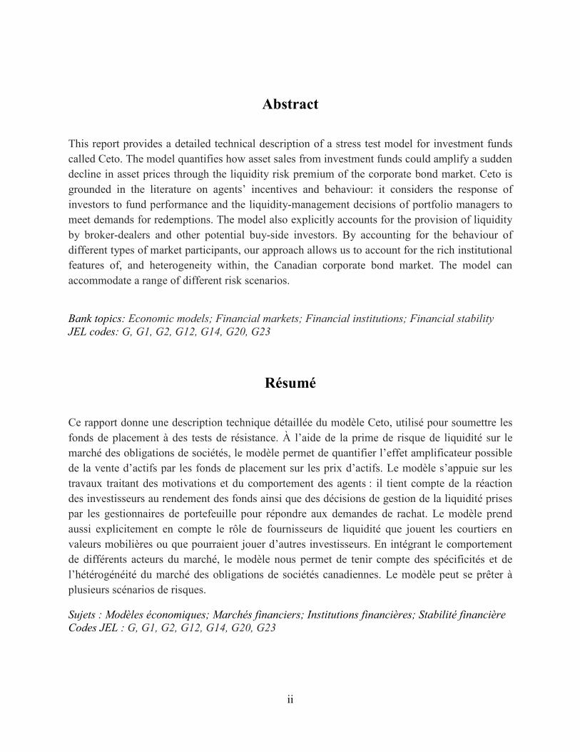
The BD’s funding cost is described by the following formula:
𝐹𝐹𝐶𝐶 = 𝑟𝑟𝑓𝑓 + ℎ𝑚𝑚_𝐵𝐵𝐷𝐷 × (𝐿𝐿𝑃𝑃𝐵𝐵𝐷𝐷 × 𝐿𝐿𝐿𝐿𝑃𝑃𝐵𝐵𝐷𝐷) + 𝐶𝐶𝐹𝐹𝑠𝑠𝑡𝑡𝐿𝐿𝐿𝐿 + 𝐶𝐶𝐹𝐹𝑠𝑠𝑡𝑡𝐿𝐿𝐿𝐿𝐿𝐿 + 𝐶𝐶𝐹𝐹𝑠𝑠𝑡𝑡𝑁𝑁𝑁𝑁𝑁𝑁𝐿𝐿_𝐿𝐿𝐶𝐶𝐷𝐷𝐶𝐶 (8)
where
• rf: risk-free rate • hm_BD: repo collateral haircut charged to the BD • PDBD: BD’s own probability of default • LGDBD: BD’s own expected loss given default • CostLR: capital charge associated with the leverage ratio • CostLCR: cost of holding liquid asset buffers against repo borrowing due to the liquidity coverage
ratio (LCR) • CostNSFR_Corp: cost of term funding associated with corporate bonds due to the net stable funding
ratio (NSFR)
Since funding is collateralized in a repo transaction, the funding cost captures the risk-free rate rf, the quality of the collateral via the haircut hm_BD, and the BD’s counterparty risk (PDBD times LGDBD).21 To calibrate the haircut hm_BD, we assume that the BD pledges only government securities as repo collateral. This is consistent with the fact that Government of Canada bonds, provincial bonds and Crown corporation debt account for 97 per cent of collateral used in the Canadian repo market (Garriott and Gray 2016). See Chart B-5 in the Appendix for a breakdown of BD’s repo collateral with non-BD counterparties.
Chart 19 shows that the funding cost rises non-linearly with the BD’s probability of default. In the LSM, the funding cost (equation 8) also accounts for costs associated with the implementation of Basel III reforms (see Box 2).
20 A repo is essentially a collateralized loan where the borrower secures the loan by posting a security as collateral. For more information on the Canadian repo market and its role in market making, see Garriott and Gray (2016) and Fontaine, Garriott and Gray (2016). 21 The BD’s probability of default is based on the structural approach of the Merton (1974) model and the Black and Scholes (1973) option pricing model.
0
1
2
3
0 1 2 3 4 5 6 7 8 9 10
%
Broker-dealer's probability of default
Chart 19: Broker-dealer's funding cost increases with increase in probability of defaults

22
Box 2 Broker-dealer’s funding cost captures new regulatory costs We describe the regulatory costs incurred by the BD to be compliant with Basel III leverage and liquidity requirements. First, the leverage ratio increases the cost of using one’s balance sheet for market-making activities.22 This cost (in basis points) is represented by
𝐶𝐶𝐹𝐹𝑠𝑠𝑡𝑡𝐿𝐿𝐿𝐿 =𝐿𝐿𝑅𝑅𝐿𝐿 × (𝛼𝛼 × 𝑄𝑄𝐵𝐵𝐷𝐷) × 𝐶𝐶
100 (9)
where • 𝛼𝛼 : proportion of unhedged bond inventory • C: cost of equity • LRT: leverage ratio target by the BD • 𝑄𝑄𝐵𝐵𝐷𝐷: quantity of corporate bonds purchased by the BD
New corporate bonds bought by the BD (QBD) increase the size of its balance sheet and the resulting cost (CostLR) to meet the Basel III leverage ratio. Chart C-2 in the Appendix shows how CostLR responds to a change in QBD.
Second, there are additional costs associated with Basel III liquidity requirements, i.e., the liquidity coverage ratio (LCR) and the net stable funding ratio (NSFR).23
• The BD must hold high-quality liquid assets (HQLA) against its repo positions. As mentioned before, we assume that the BD’s repo transactions are made against highly liquid bonds, resulting in a relatively small incremental cost. This cost is calibrated as well (see Table A-2 in the Appendix for the calibration).
• In contrast to the LCR, the cost associated with the NSFR (CostNSFR_Corp) is more significant. CostNSFR_Corp is specified as follows:
𝐶𝐶𝐹𝐹𝑠𝑠𝑡𝑡𝑁𝑁𝑁𝑁𝑁𝑁𝐿𝐿_𝐿𝐿𝐶𝐶𝐷𝐷𝐶𝐶 =𝑄𝑄𝐵𝐵𝐷𝐷 × 𝑀𝑀𝑀𝑀𝑀𝑀 �0,𝑅𝑅𝑆𝑆𝐹𝐹𝐿𝐿𝐶𝐶𝐷𝐷𝐶𝐶 −
𝐸𝐸𝐵𝐵𝑆𝑆� × 𝑅𝑅𝑅𝑅𝑅𝑅𝐹𝐹𝑠𝑠𝐶𝐶𝐷𝐷𝑒𝑒𝑠𝑠𝑠𝑠
10 (10)
where • 𝑄𝑄𝐵𝐵𝐷𝐷: corporate bonds purchased by the BD • 𝑅𝑅𝑆𝑆𝐹𝐹𝐿𝐿𝐶𝐶𝐷𝐷𝐶𝐶: required stable funding factor for corporate bonds • E: BD’s Tier 1 equity capital • BS: BD’s balance sheet size • 𝑅𝑅𝑅𝑅𝑅𝑅𝐹𝐹𝑠𝑠𝐶𝐶𝐷𝐷𝑒𝑒𝑠𝑠𝑠𝑠: yield on the one-month Canadian repo rate minus yield on one-month treasury bills
In the LSM, the increase in the BD’s balance sheet associated with the purchase of corporate bonds leads to an increase in required stable funding (RSF). To calibrate the RSFCorp factor, we assume that the corporate bonds purchased from funds are held for less than six months on its balance sheet (see Table D-1 and Table D-2 in the Appendix for more details on the RSF and available stable funding [ASF] calibrations). We deduct equity capital as it qualifies fully as stable funding (RSF=1). We then multiply this required stable funding by the one-month repo spread to obtain the NSFR cost. Chart C-2 in the Appendix shows the linear relationship between the amount of corporate bonds purchased by the BD (QBD) and the cost associated with the NSFR (CostNSFR_Corp).
22 In contrast to the risk-weighted capital requirements, the leverage ratio requires banks to hold capital against their unweighted balance sheet risk exposures (i.e., assets, derivatives and off-balance-sheet exposures). 23 The LCR requires banks to hold an adequate stock of HQLA relative to estimated stressed net cash outflows over the next 30 calendar days. The NSFR requires banks to fund their activities with sufficiently stable sources of funding. The NSFR defines the amount of available stable funding (ASF) relative to the amount of required stable funding (RSF).
23
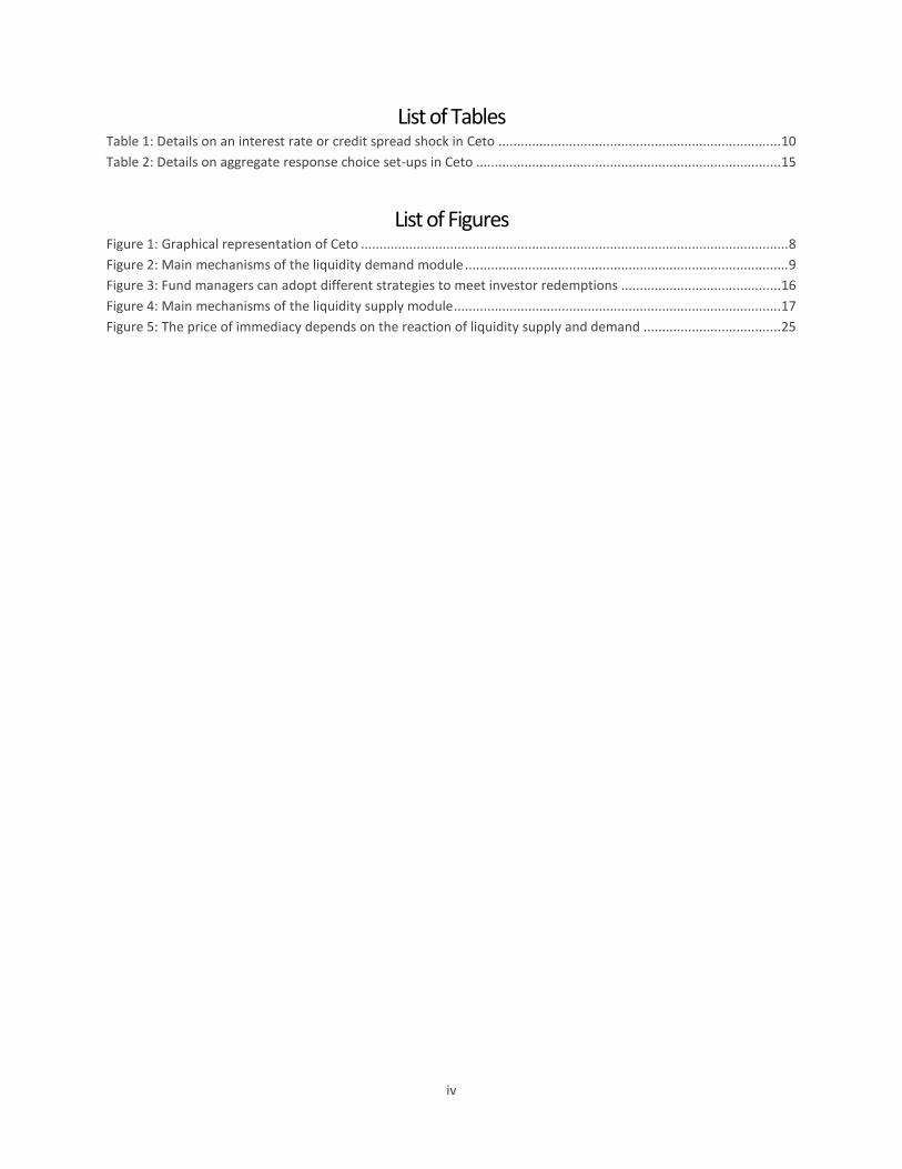
So far, we have shown that the price component (cost-benefit trade-off) is an important factor in the BD’s decision to supply liquidity. The rest of this subsection describes the other important factor, the quantity component. In the LSM, liquidity provision by the BD also relates to its risk-bearing capacity, i.e., its ability and willingness to increase its holdings of corporate bonds. The BD could become reluctant to warehouse large positions during periods of high volatility if it approaches internal risk limits. In response, the BD could reduce its market-making volumes (instead of just adjusting quoted prices).24 This dimension is important in our model because bank-owned broker-dealers scaled back their market-making activities post-crisis, reflecting lower risk appetites and the impact of regulatory changes (e.g., Basel III requirements).
In the LSM, the BD’s risk-bearing capacity (RBC) depends on its capital base, the leverage ratio and market volatility.25 RBC is represented by:
𝑅𝑅𝐵𝐵𝐶𝐶 = (𝐸𝐸 × 𝐿𝐿𝑅𝑅𝐿𝐿) − 𝐵𝐵𝑆𝑆 (11)
where
• RBC: BD’s risk-bearing balance sheet capacity • E: BD’s Tier 1 equity capital • LRT: leverage ratio target for the BD • BS: BD’s leverage ratio balance sheet exposure
In equation 11, market volatility (proxied by the Chicago Board Options Exchange Volatility Index [VIX]) negatively affects BD’s capital and leverage risk-bearing capacities (see Table A-2 in the Appendix for more details on the estimated relationships), reflecting the higher probability that the BD could incur losses on its assets. Moreover, risk tolerance declines in times of stress. Chart 20 shows the relationship between a rise in the VIX and BD’s risk-bearing balance sheet capacity. An increase in market stress causes the BD to reduce the amount of risk capital it allocates to market intermediation. This behaviour in the LSM is plausible because in previous episodes of market stress, broker-dealers have acted strategically to protect their balance sheets and have hoarded liquidity (Committee on the Global Financial System 2016).
Finally, the BD typically operates with a buffer over the regulatory leverage requirement minimum, and we calibrate the leverage ratio target as such in the LSM (See Table A-2 in the Appendix).
Providing financing through reverse repo to the long-term investor
24 The difference between actual and desired or targeted inventory levels is important to a BD, who must comply with internal risk limits. 25 In Canada, the dealer subsidiaries of the six Canadian domestic systemically important banks (DSIBs) are the most important market makers in fixed-income markets. However, we do not have data on dealer subsidiaries’ balance sheets, hindering our ability to look at types and quantity of assets held in inventory. Due to this constraint, the representative dealer in the LSM is calibrated based on the consolidated balance sheets of the DSIBs. Table A-2 in the Appendix provides details about the calibration.
-200
0
200
400
600
1 5 9 13 17 21 25 29
$ billions
Increase in VIX
Chart 20: Broker-dealer's risk-bearing balance sheet decreases with an increase in the VIX
24
In the LSM, the BD also provides short-term funding (through reverse repo) to the LTI. In the LSM, the repo rate charged by the BD to the LTI reflects the marginal cost associated with the transaction, i.e., the risk-free rate, a haircut, LTI’s credit risk and the cost of capital associated with liquidity requirements.
The repo rate is described by the following formula:
𝑅𝑅 = 𝑟𝑟𝑓𝑓 + ℎ𝑚𝑚_𝐿𝐿𝑇𝑇𝐿𝐿 × (𝐿𝐿𝑃𝑃𝐿𝐿𝑇𝑇𝐿𝐿 × 𝐿𝐿𝐿𝐿𝑃𝑃𝐿𝐿𝑇𝑇𝐿𝐿) + 𝐶𝐶𝐹𝐹𝑠𝑠𝑡𝑡𝑁𝑁𝑁𝑁𝑁𝑁𝐿𝐿_𝐿𝐿𝑒𝑒𝑅𝑅 (12)
where
• hm_LTI: repo collateral haircut charged to the LTI • PDLTI: LTI’s probability of default • LGDLTI: LTI’s expected loss given default • CostNSFR_Rev: cost of term funding required for reverse repo under the net stable funding ratio
In our model, the BD lends cash to the LTI and obtains collateral in return. The repo rate captures the treatment of reverse repo transactions and their impact on the NSFR.26 To calibrate the RSF factor in equation 13, we assume that the BD provides funding for less than six months (see Table A-2 in the Appendix).27 Reverse repo decreases the net stable funding, which is equivalent to the BD’s cost of NSFR (CostNSFR_Rev) for reverse repo transaction. CostNSFR_Rev is specified as follows:
𝐶𝐶𝐹𝐹𝑠𝑠𝑡𝑡𝑁𝑁𝑁𝑁𝑁𝑁𝐿𝐿_𝐿𝐿𝑒𝑒𝑅𝑅 =𝑄𝑄𝐿𝐿𝑇𝑇𝐿𝐿 ×𝑀𝑀𝑀𝑀𝑀𝑀 �0,𝑅𝑅𝑆𝑆𝐹𝐹𝐿𝐿𝑒𝑒𝑅𝑅𝑒𝑒𝐷𝐷𝑠𝑠𝑒𝑒 −
𝐸𝐸𝐵𝐵𝑆𝑆�× 𝑅𝑅𝑅𝑅𝑅𝑅𝐹𝐹𝑠𝑠𝐶𝐶𝐷𝐷𝑒𝑒𝑠𝑠𝑠𝑠
10 (13)
where
• 𝑄𝑄𝐿𝐿𝑇𝑇𝐿𝐿: corporate bonds purchased by the LTI • 𝑅𝑅𝑆𝑆𝐹𝐹𝐿𝐿𝑒𝑒𝑅𝑅𝑒𝑒𝐷𝐷𝑠𝑠𝑒𝑒: RSF factor for reverse repo
Cost associated with leverage does not apply in equation 13 because reverse repo has no impact on the BD’s balance sheet. Therefore, the BD’s leverage ratio and capital requirements are unaffected.
Impact on market through the liquidity risk premium Ceto operates sequentially to quantify the impact of bond funds’ asset liquidation on corporate bond market liquidity: the output of the liquidity demand module—i.e., sales of corporate bonds by investment funds (Q)—is used as an input in the LSM, which drives the decisions of both the LTI and the BD to acquire corporate bonds.28 As shown in Figure 5, Ceto’s main output is the impact on liquidity conditions in the corporate bond market as measured by the liquidity risk premium.29
The liquidity risk premium quantifies the net impact of the interaction of demand for and supply of immediacy (Figure 4). For example, the materialization of a stress event (e.g., interest rate shock) increases demand for immediacy by bond managers as they adjust portfolios to meet redemptions (i.e., demand curve shifts right in Figure 5). Ceteris paribus, the resulting sales of corporate bonds, which is the output of the LDM, exert upward pressure on the price of immediacy. In response, potential liquidity
26 This is because the cash is converted into receivables, which require stable funding (RSF equals 10 per cent). At the same time, the BD receives collateral, which is kept off the balance sheet and has no impact on ASF and RSF. 27 This maturity assumption in the LSM is consistent with the fact that roughly 80 per cent of all reverse repo transactions in Canada are shorter than 91 days (Garriott and Gray 2016). 28 In contrast, asset sales by investment funds are exogenous in Baranova, Liu and Shakir (2017).
29 The liquidity risk premium informs whether the Canadian bond market is resilient and would continue functioning in situations of market stress. But it cannot evaluate another dimension of market resilience, i.e., the time it takes for prices to return to fundamental value in response to a shock.

25
providers in the LSM can satisfy bond fund managers’ demand for immediacy by buying corporate bonds. Supply’s response to a demand shock determines the market-clearing price of immediacy while accounting for two types of potential buyers and their corresponding interactions. As an example, if supply does not adjust quickly, the price of immediacy (liquidity risk premium) is pushed higher and leads to deterioration in market liquidity (Figure 5).
Figure 5: The price of immediacy (liquidity risk premium) depends on the reaction of liquidity supply and demand
In Ceto, equilibrium is achieved as follows. First, for a given sale of corporate bonds by fund managers (Q), the representative BD absorbs the residual amount (QBD = Q – QLTI) that is not purchased by the representative LTI (QLTI). Second, the module estimates the increase in the liquidity risk premium over one quarter given the amount of corporate bonds being purchased by the BD (QBD). Intuitively, a reduction in BD’s risk tolerance to taking larger positions will be reflected in the liquidity risk premium, providing greater incentives to the LTI to provide liquidity. The LSM assumes that the representative BD sets the market clearing price (consistent with Kyle 1985), implying that the LTI corporate bond purchase (QLTI) is executed at the same price discount (liquidity risk premium) as the BD purchase (QBD) (see Figure 5).
5 Model limitations A model is an investigative framework that helps fit theories to data; as such, it is a simplification of the real world. Ceto is no different in this regard and faces its share of model limitations. This section discusses these limitations in greater depth and posits potential enhancements that could be incorporated in future generations of Ceto. This section’s structure is similar to the presentation of Ceto in this report: it begins by discussing limitations associated with data, then explains both the limitations of each module and potential future work and finishes by underlining restrictions faced by the overall stress-testing framework.
5.1 Data limitations Morningstar Direct is Ceto’s primary data source for fund-level asset allocation, fund-level allocation by credit quality, fund duration and other fund characteristics. On the other hand, Morningstar holdings data, joined with Thompson Reuters’ fixed-income dataset, are used for data validation and for computing fund-level asset allocation to a particular asset subclass—Canadian corporate debt denominated in Canadian dollars. Morningstar holdings data serve as a secondary data source.
P*
Q*
Price of immediacy
Sales of corporate bonds
Supply of immediacy
Demand for immediacy
Price of immediacy
Sales of corporate bonds
Supply of immediacy
Demand for immediacy
Q*
P*
Q
P

26
Future versions of Ceto could be improved by relying directly on Morningstar holdings data as a primary data source. Holdings data provide greater granularity and consequently can be used to construct bottom-up metrics on asset allocation, which allows for better classification of funds between fixed-income and mixed categories. Also, holdings data can be used to measure portfolio turnover, a metric that can be used as a proxy for active management, again allowing for better classification of funds between active and indexed categories. Furthermore, as stated in Section 4.1.2 (footnote 7), LDM currently operates on the assumption that duration does not vary by credit quality, a shortcoming that can be addressed by calculating duration by credit quality from holdings data. Finally, for a given risk scenario, LDM currently breaks down outflow composition into major asset classes: cash and cash equivalents, equities, government bonds, corporate bonds, and others. A move towards holdings data as a primary data source will allow for greater granularity in outflow composition. Outflows could be broken down by (i) asset subclasses, for example, separating government bond outflows into sovereign versus provincial debt; (ii) asset issuer, for example, dividing corporate bond outflows into financial versus non-financial corporate debt; (iii) maturity structure, for example, segregating bond outflows by remaining maturity at time of sale; and (iv) credit quality, for example, partitioning bond outflows into high-yield and investment-grade debt. Detailed outflow compositions could help in better identifying subsectors of the overall Canadian corporate bond market that could come under stress if the risk scenario materializes.
5.2 Limitations—liquidity demand module The LDM, which quantifies the amount of assets sold by bond funds for a given risk scenario, faces limitations that could be addressed in future versions. First, the interest rate risk scenario in LDM allows only for parallel movements of the yield curve. This constraint emanates from the use of a single interest rate sensitivity metric—fund duration. The interest rate risk scenario in LDM could be made more dynamic by using key rate durations for each fund’s portfolio.30 Key rate durations at specific maturities for each fund portfolio would allow for more complex interest rate risk scenarios, such as steepening and flattening of the yield curve. Second, in LDM, liquidity management strategies employed by fund managers are based on heuristics: vertical selling, horizontal selling and mixed selling. These heuristics are informative as they highlight the effect of fund manager behaviour on the composition of assets sold (see Section 4.1.4). However, these heuristics ignore extraordinary liquidity management tools, such as gating and NAV swing pricing, that may be employed by fund managers in the face of large and unexpected redemptions. These unconventional tools can affect the composition of assets sold, ultimately impacting the demand for liquidity by bond funds in the corporate bond market. Malik and Lindner (2017) and Lewrick and Schanz (2017) provide econometric and theoretical frameworks for NAV swing pricing that could be incorporated in future versions of Ceto.
5.3 Limitations—liquidity supply module The LSM, which quantifies the impact of bond fund sales through the liquidity risk premium in the Canadian corporate bond market, also faces shortcomings that may be addressed in the future.
First, LSM is a two-agent model with a representative long-term investor and a representative broker-dealer; as such, LSM lacks heterogeneity in terms of economic agents. Future versions of LSM could include a richer variety of long-term investors, such as insurance companies, pension funds and hedge
30 Key rate duration measures the change in value of a fund’s asset holdings for a change in interest rate at a particular maturity on the yield curve while keeping the rest of the yield curve constant.

27
funds with unique objective functions and liquidity constraints. A heterogenous set of long-term investors would better reflect the Canadian corporate bond market and, consequently, give a more accurate picture of the ability of long-term investors to supply liquidity in periods of market stress. Douglas and Roberts-Sklar (2018) and Douglas, Noss and Vause (2017) model the behaviour of UK pension funds and UK insurance companies, respectively. Their frameworks could potentially be used to address this shortcoming in the LSM.
Second, LSM computes liquidity risk premium for only the Canadian corporate bond market. However, the composition of assets sold includes another fixed-income asset, namely government bonds. In Ceto, government bond sales include sovereign bonds (Government of Canada securities) and provincial bonds. While liquidity in the Canadian sovereign bond market has historically been resilient, it has deteriorated during stressful events, such as the taper tantrum of 2013 and the oil price shock of 2015, as shown by Gungor and Yang (2017). Fan et al. (2018) discover similar results for resilience of liquidity in the Canadian provincial bond market. Therefore, LSM could be extended to calculate liquidity risk premiums in all three fixed-income markets, i.e., corporate, federal, and provincial government bond markets.
5.4 Limitations—Ceto framework As the previous two subsections highlight specific limitations in each module, this subsection will address a model constraint that is more global in nature.
Ceto is a single-period stress-testing framework. In Ceto, the risk scenario lowers bond prices, resulting in outflows from bond funds. These outflows represent demand for liquidity in the Canadian corporate bond market and generate an associated liquidity risk premium. Ceto stops after the generation of the liquidity risk premium; however, this risk premium represents an additional decline in bond prices separate from the risk scenario. This additional decline could generate a second round of bond fund outflows—a feedback effect. Ceto does not model this feedback effect, which would last over multiple periods. These second-round effects are important because they reinforce the first-mover advantage and capture the run dynamic that may be experienced by bond funds during periods of heighted bond market volatility (Chen, Goldstein and Jiang 2010).
Ceto is the Bank of Canada’s first investment fund stress-testing framework; therefore, it was kept relatively parsimonious and tractable to permit modelling of important and well-understood financial channels. Future generations of Ceto, and Ceto-like models, will address limitations outlined in this technical report.
6 Conclusion Risk-assessment models are an important component of the Bank of Canada’s analytical tool kit for assessing the resilience of the financial system. This technical report presents Ceto, a new stress-testing model for investment funds. Ceto quantifies the effects of collective selling by investment funds on fixed-income market liquidity in a severe but plausible risk scenario.
This quantitative assessment is important because market-based intermediaries such as investment funds are playing a more important role in credit intermediation since the global financial crisis (Bédard-Pagé 2019). In addition to quantification, Ceto also allows us to better understand channels through which financial shocks could be amplified by investment funds. Thus, Ceto provides a necessary analytical tool to assess vulnerabilities in this sector and to inform policy decisions related to financial stability.
Future work on developing Ceto will focus on designing more flexible risk scenarios (e.g., a non-parallel shift in the yield curve) as well as refinements to the behaviour of other market participants. In particular,

28
the key factors driving the rebalancing decisions of institutional investors and their ability and willingness to invest counter-cyclically remain a matter of debate. As we further refine our understanding of the interplay between these factors, future improvements to the model will remove some of the restrictions on model dynamics currently assumed in Ceto.

29
References
Anand, A. and K. Venkataraman. “Market Conditions, Fragility and the Economics of Market Making.” Journal of Financial Economics (forthcoming).
Arora, R. 2018. “Redemption Runs in Canadian Corporate Bond Funds?” Bank of Canada Staff Analytical Note No. 2018-21.
Arora, R., C. Fan and G. Ouellet Leblanc. 2019. “Liquidity Management of Canadian Corporate Bond Mutual Funds: A Machine Learning Approach.” Bank of Canada Staff Analytical Note No. 2019-7.
Arora, R. and G. Ouellet Leblanc. 2018. “How Do Canadian Corporate Bond Mutual Funds Meet Investor Redemptions?” Bank of Canada Staff Analytical Note No. 2018-14.
Bank of England. 2014. “Procyclicality and Structural Trends in Investment Allocation by Insurance Companies and Pension Funds: A Discussion Paper by the Bank of England and the Procyclicality Working Group.”
Baranova, Y., J. Coen, P. Lowe, J. Noss and L. Silvestri. 2017. “Simulating Stress Across the Financial System: The Resilience of Corporate Bond Markets and the Role of Investment Funds.” Bank of England Financial Stability Papers No. 42.
Baranova, Y., Z. Liu and T. Shakir. 2017. “Dealer Intermediation, Market Liquidity and the Impact of Regulatory Reform.” Bank of England Working Paper No. 665.
Barras, L., O. Scaillet and R. Wermers. 2010. “False Discoveries in Mutual Fund Performance: Measuring Luck in Estimated Alphas.” The Journal of Finance 65 (1): 179–216.
Bédard-Pagé, G. 2019. “Non-Bank Financial Intermediation in Canada: An Update.” Bank of Canada Staff Discussion Paper No. 2019-2.
Bédard-Pagé, G., A. Demers, E. Tuer and M. Tremblay. 2016. “Large Canadian Public Pension Funds: A Financial System Perspective.” Bank of Canada Financial System Review (June): 33–38.
Ben-Rephael, A., S. Kandel and A. Wohl. 2012. “Measuring Investor Sentiment with Mutual Fund Flows.” Journal of Financial Economics 104 (2): 363–382.
Black, F. and M. Scholes. 1973. “The Pricing of Options and Corporate Liabilities.” Journal of Political Economy 81 (3): 637–654.
Braun-Munzinger, K., Z. Liu and A. Turrell. 2016. “An Agent-Based Model of Dynamics in Corporate Bond Trading.” Bank of England Staff Working Paper No. 592.
Brunnermeier, M. K. and L. H. Pedersen. 2009. “Market Liquidity and Funding Liquidity.” Review of Financial Studies 22 (6): 2201–2238.
Cetorelli, N., F. Duarte and T. Eisenbach. 2016. “Are Asset Managers Vulnerable to Fire Sales?” Liberty Street Economics (blog), Federal Reserve Bank of New York. February 18, 2016.
Chen, Q., I. Goldstein and W. Jiang. 2010. “Payoff Complementarities and Financial Fragility: Evidence from Mutual Fund Outflows.” Journal of Financial Economics 97 (2): 239–262.

30
Chernenko, S. and A. Sunderam. 2016. “Liquidity Transformation in Asset Management: Evidence from the Cash Holdings of Mutual Funds.” European Systemic Risk Board Working Paper No. 23.
Chevalier, J. and G. Ellison. 1997. “Risk Taking by Mutual Funds as a Response to Incentives.” Journal of Political Economy 105 (6): 1167–1200.
Choi, J. and O. Shachar. 2013. “Did Liquidity Providers Becomes Liquidity Seekers?” Federal Reserve Bank of New York Staff Report No. 650.
Choi, J., O. Shachar and S. S. Shin. 2018. “Dealer Liquidity Provision and the Breakdown of the Law of One Price: Evidence from the CDS-Bond Basis.” Management Science (July).
Christensen I., G. Kumar, C. Meh and L. Zorn. 2015. “Assessing Vulnerabilities in the Canadian Financial System.” Bank of Canada Financial System Review (June): 37–46.
Committee on the Global Financial System. 2016. “Fixed Income Market Liquidity.” CGFS Papers No. 55. Bank for International Settlements.
Coval, J. and E. Stafford. 2007. “Asset Fire Sales (and Purchases) in Equity Markets.” Journal of Financial Economics 86 (2): 479–512.
Diamond, D. and P. Dybvig. 1983. “Bank Runs, Deposit Insurance, and Liquidity.” Journal of Political Economy 91 (3): 401–419.
Dick-Nielson, J. and M. Rossi. 2018. “The Cost of Immediacy for Corporate Bonds.” The Review of Financial Studies 32 (1): 1–41.
Dick-Nielsen, J., P. Feldhütter and D. Lando. 2012. “Corporate Bond Liquidity Before and After the Onset of the Subprime Crisis.” Journal of Financial Economics 103 (3): 471–492.
Douglas, G., J. Noss and N. Vause. 2017. “The Impact of Solvency II Regulations on Life Insurers’ Investment Behaviour.” Bank of England Staff Working Paper No. 664.
Douglas, G. and M. Roberts-Sklar. 2018. “What Drives UK Defined Benefit Pension Funds’ Investment Behaviour?” Bank of England Staff Working Paper No. 757.
Elton, E., M. Gruber and C. Blake. 1996. “The Persistence of Risk-Adjusted Mutual Fund Performance.” The Journal of Business 69 (2): 135–157.
European Central Bank. 2017. Financial Stability Review (May).
Fan C., S. Gungor, G. Nolin and J. Yang. 2018. “Have Liquidity and Trading Activity in the Canadian Provincial Bond Market Deteriorated?” Bank of Canada Staff Analytical No. 2018-30.
Financial Stability Board (FSB). 2017. “Policy Recommendation to Address Structural Vulnerabilities from Asset Management Activities.”
———. 2019. Global Monitoring Report on Non-Bank Financial Intermediation 2018.

31
Fontaine, J.-S., C. Garriott and K. Gray. 2016. “Securities Financing and Bond Market Liquidity.” Bank of Canada Financial System Review (June): 39–45.
Fricke, C. and D. Fricke. 2017. “Vulnerable Asset Management? The Case of Mutual Funds.” Deutsche Bundesbank Discussion Paper No. 32/2017.
Garriott, C. and K. Gray. 2016. “Canadian Repo Market Ecology.” Bank of Canada Staff Discussion Paper No. 2016-8.
Garriott, C. and J. Johal. 2018. “Customer Liquidity Provision in Canadian Bond Markets.” Bank of Canada Staff Analytical Note No. 2018-12.
Goldstein, I., H. Jiang and D. T. Ng. 2017. “Investor Flows and Fragility in Corporate Bond Funds.” Journal of Financial Economics 126 (3): 592–613.
Greenwood, R., A. Landier and D. Thesmar. 2015. “Vulnerable Banks.” Journal of Financial Economics 115 (3): 471–485.
Grinblatt, M. and S. Titman. 1989. “Mutual Fund Performance: An Analysis of Quarterly Portfolio Holdings.” The Journal of Business 62 (3): 393–416.
———. 1993. “Performance Measurement Without Benchmarks: An Examination of Mutual Fund Returns.” The Journal of Business 66 (1): 47–68.
Gullapalli, D., S. Anand and D. Maxey. 2008. “Money Fund, Hurt by Debt Tied to Lehman, Breaks the Buck.” The Wall Street Journal, September 17, 2008. Accessed March 5, 2019. https://www.wsj.com/articles/SB122160102128644897
Gungor, S. and J. Yang. 2017. “Has Liquidity in Canadian Government Bond Markets Deteriorated?” Bank of Canada Staff Analytical Note No. 2017-10.
Hyun, D., J. Johal and C. Garriott. 2017. “Do Canadian Broker-Dealers Act as Agents or Principals in Bond Trading?” Bank of Canada Staff Analytical Note No. 2017-11.
Jiang, H., D. Li and A. Wang. 2017. “Dynamic Liquidity Management by Corporate Bond Mutual Funds.” Available at SSRN: https://ssrn.com/abstract=2776829
Kozicki, S. and J. Vardy. 2017. “Communicating Uncertainty in Monetary Policy.” Bank of Canada Staff Discussion Paper No. 2017-14.
Kyle, A. 1985. “Continuous Auctions and Insider Trading.” Econometrica 53 (6): 1315–1336.
Lewrick, U. and J. Schanz. 2017. “Is the Price Right? Swing Pricing and Investor Redemptions.” BIS Working Paper No. 664. Bank for International Settlements.
Malik, S. and P. Lindner. 2017. “On Swing Pricing and Systemic Risk Mitigation.” International Monetary Fund Working Paper No. 17/159.
Merton, R. 1974. “On the Pricing of Corporate Debt: The Risk Structure of Interest Rates.” The Journal of Finance 29 (2): 449–470.

32
Morris, S., I. Shim and H. S. Shin. 2017. “Redemption Risk and Cash Hoarding by Asset Managers.” BIS Working Paper No. 608. Bank for International Settlements.
Nagel, S. 2012. “Evaporating Liquidity.” The Review of Financial Studies 25 (7): 2005–2039.
Organisation for Economic Co-operation and Development (OECD). 2019. “Corporate Bond Markets in a Time of Unconventional Monetary Policy.” OECD Capital Market Series.
Office of Financial Research. 2016. 2016 Annual Report to Congress.
Sharpe, W. 1966. “Mutual Fund Performance.” The Journal of Business 39: 119–138.
Sirri, E. R. and P. Tufano. 1998. “Costly Search and Mutual Fund Flows.” The Journal of Finance 53 (5): 1589–1622.
Timmer, Y. 2017. “Cyclical Investment Behaviour across Financial Institutions.” ECMI Working Paper No. 4. European Capital Markets Institute.
Weill, P.-O. 2007. “Leaning Against the Wind.” The Review of Economic Studies 74 (4): 1329–1354.

33
Appendix A Table A-1: Liquidity demand module variables and data sources
Variables Description Source Computation and units Broad-based asset allocation
Share of allocation towards cash, bonds, equity and other
Morningstar Direct
In percentage points
Credit-quality allocation
Share of fixed-income allocation towards credit-quality ratings: AAA, AA, A, BBB, BB, B and below B
Morningstar Direct
In percentage points
Fund flows Monthly fund flows aggregated from share classes
Morningstar Direct
In percentage points. Winsorized at 1 and 99 percentiles
Equity market value The total market value of all equity held by a fund
Morningstar Direct
As stated in Canadian dollars
Fixed-income market value
The total market value of all fixed income held by a fund
Morningstar Direct
As stated in Canadian dollars
Total market value The total market value of the fund
Morningstar Direct
As stated in Canadian dollars
Fund size Total fund size aggregated from share classes (proxy for book value)
Morningstar Direct
As stated in Canadian dollars
Share class inception date
The date when the share class was created
Morningstar Direct
Date as stated
Share class obsolescence
The date when the share class became obsolete
Morningstar Direct
Date as stated
Modified duration The average modified duration of the fund
Morningstar Direct
As stated
Returns The gross and net monthly returns for share classes
Morningstar Direct
In percentage points
Equity market return S&P 500 total market return Global Financial Data
In percentage points
Risk-free rate 1-month US Treasury rate Federal Reserve Bank of St. Louis FRED (Federal Reserve Economic Data)
In percentage points

34
Table A-2: Calibration of the liquidity supply module: variables and data sources Variables Description Value Sources Computation and units Q Size of the sale
of corporate bonds
2007: 5.0 2018: 31.7
Output of the liquidity demand module
In CAD billions, function of the liquidity-management strategy
𝛼𝛼 Proportion of unhedged bond inventory
2007: 0.5 2018: 0.2
Market intelligence and expert judgement
Proportion of BD’s bond inventory that is unhedged
LRT Leverage ratio target
2007: 0.03 2018: 0.04
Regulatory filings of Canadian banks and Bank of Canada calculations
In percentage points. Based on Canadian DSIBs’ balance sheets. We compute the weighted-average value for the representative broker-dealer.
C Cost of equity 2007: 8.09 2018: 11.33
Bloomberg In percentage points
Initial RWAM Market risk-weighted assets (RWA) of the representative broker-dealer
2007: 5.0 2018: 6.7
Regulatory filings of Canadian banks, Bank of Canada calculations, Basel Capital Adequacy Reporting returns
In CAD billions
RWAM Market RWA based on the Chicago Board Options Exchange Volatility Index (VIX) increase
InitialRWAM + ((0.0001749*VIX^2) + (0.000071*VIX) + 0.00803)
Bank of Canada calculations
In CAD billions
rf 1-month yield on Canadian treasury bills
2007: 4.10 2018: 1.92
Bank of Canada
In percentage points
hBD Haircut on dealer repo borrowing
2007: VIX+(2.2*0.0212) 2018: VIX+(2.2*0.003)
Bloomberg In percentage points
LGDBD Loss given default for the representative broker-dealer
0.4 Expert judgement
In percentage points

35
Variables Description Value Sources Computation and units LGDLTI Loss given
default for the representative long-term investor
0.4 Expert judgement
In percentage points
LCRcost Cost of borrowing Canadian government bonds
2007: 0 bps 2018: 5 bps
IHS Markit In percentage points. Based on the cost of borrowing government bonds in the securities lending market. In 2007, the value is set to 0 bps because the LCR was not yet implemented.
RSFReverse Net stable funding ratio (NSFR) required stable funding (RSF) factor for reverse repo
2007: 0.0 2018: 0.1
Office of the Superintendent of Financial Institutions (OSFI)
Average of RSF factor for reverse repo, maturity lower than 6 months (see Table D-2 in the Appendix)
RSFCorp NSFR RSF factor for corporate bonds
2007: 0.0 2018: 0.5
OSFI The RSF factor NSFR_Corp assigned to corporate bonds is 0.5 according to the Basel III NSFR requirements if the maturity is less than 6 months or between 6 and 12 months (Table D-2 in the Appendix). In the LSM, BD’s repo transaction to fund the purchase of corporate bonds does not affect the cost of NSFR because we assume that the cash is borrowed from bank-owned broker-dealers for a maturity shorter than 6 months. According to the NSFR rules, the repo financing does not provide stable funding (ASF = 0%), while the cash received does not require additional funding (RSF = 0%) (Table D-1 and Table D-2 in the Appendix).
E Tier 1 equity capital
2007: 88 2018: 239
Regulatory filings of Canadian banks
In CAD billions

36
Variables Description Value Sources Computation and units BS Leverage ratio
balance sheet exposure
2007: 3,350 2018: 5,522
Regulatory filings of Canadian banks
In CAD billions
Repospread Term premium of the Canadian repo market
2007: 16 bps 2018: 8 bps
Canadian Depository for Securities (CDS), Market Trade Reporting System 2.0 (MTRS 2.0) and Statistics Canada
Yield on 1-month Canadian repo rate minus yield on the 1-month treasury bills
MLiqCorp Daily liquidation amount of corporate bonds (sell initiated)
2007: 287 2018: 725
CDS and Bank of Canada calculations. (See Fan, Gungor, Nolin and Yang 2018)
Daily liquidation amount of corporate bonds by market maker
HPBD The expected holding period of the broker-dealer
QBD/MLiqCorp CDS The expected inventory holding period is calculated by dividing the size of the purchase by the [daily, quarterly] liquidation amount.
S Broker-dealer bid-ask spread
2007: 30 2018: 45
CDS and Bank of Canada calculations
In basis points. Calibrated using episodes in our dataset when liquidity of the corporate bond market has deteriorated.
ULA Amount of unencumbered liquid assets
75 Market intelligence
In CAD billions
hLTI Haircut on long-term investor repo borrowing
(0.001*VIX)-0.0021 Bloomberg In percentage points

37
Variables Description Value Sources Computation and units VIX 30-day implied
volatility S&P/TSX index (VIXC) and the Chicago Board Options Exchange Volatility Index (VIX)
2007: 17.5 2018: 13.8
Bloomberg Daily average VIXC in 2018 and the daily average VIX in 2007 since the VIXC was not available. In percentage points
HedgePremium Credit default swap premium
(0.004 + (1.613 *∆VIX)) /10000
Bloomberg Estimated linear relationship between the VIX index and credit default swap indices
HedgingSpread Spread cost of hedging
2007: 1.31 bps 2018: 1 bps
Bloomberg Bid-ask spread in the 5-year Canadian interest rate swap market. In basis points
HC
Hedging cost HPBD * (HedgePremium * QBD * (1 − 𝛼𝛼)) + HedgingSpread
Bloomberg Hedging costs include bid-ask spreads and CDS protection premium paid.

38
Appendix B
49 41
3338
14 114 10
2007 20180
20
40
60
80
100
AAA AA A BBB
Chart B-1:
Source: Bank of America Merrill Lynch
Canadian broad bond index
Last observation: September 2018
Monthly data
9277
823
2007 20180
20
40
60
80
100
BB B
Chart B-2:
Source: Bank of America Merrill Lynch
Canadian high-yield corporate bond index
Last observation: September 2018
Monthly data
5
6
7
8
2007 2009 2011 2013 2015 2017
Duration
Chart B-3: Canadian bond index modified durationQuarterly frequency
Last observation: 2018Q3Source: Bank of America
Note: Composed by taking 90 per cent of the broad Canadian bond index and 10 per cent of the high-yield Canadian corporate bond index
0
50
100
150
200
250
2007 2009 2011 2013 2015 2017
$ billions
Repurchase agreementsReverse repurchase agreements
Chart B-4: Canadian domestic bank repo activityMonthly data
Last observation: November 2018Source: Banks' regulatory filings
81
720
1
89
15
35
10
25
50
75
100$ billions
Repo Reverse repo
Chart B-5:
Last observation: July 2018Sources: MTRS 2.0 and TRITON
Broker-dealers' collateral with non-broker-dealersMonthly data
0
10
20
30
40
50
60
70
2010 2011 2012 2013 2014 2015 2016 2017 2018
bps
BanksNon-bank financial corporationsNon-financial corporations
Chart B-6: Bid-ask proxy4-week moving average, weekly data
Last observation: December 2018
Sources: Canadian Depository for Securities and Bank of Canada calculations

39
Appendix C
0
10
20
30
0 5 10 15 20 25 30 35 40
Increase in RWA
Increase in VIX
Chart C-1: Increase in risk-weighted assets (RWA) increases with VIX
0
4
8
12
0 4 8 12 16 20 24 28
Basis points
Quantity purchased by broker-dealer ($ billions)NSFR cost Leverage cost
Chart C-2: NSFR and leverage costs increase linearly with the quantity purchased by the broker-dealer

40
Appendix D Table D-1: The net stable funding ratio—available stable funding factors
Basel III: The net stable funding ratio—available stable funding factors (ASF)*
Regulatory capital
Non-maturity demand and term deposits provided by
retail and SME customers
Operational deposits
Other funding provided by Other capital
instruments Interdependent
liabilities
Stable Less stable
Corporates, sovereigns,
MDBs and PSEs
Central banks and financial
institutions Mat <6m 100 95 90 50 50 0 0 0
Mat 6-12 m 100 95 90 50 50 50 50 0
Mat ≥1 year 100 100 100 100 100 100 100 0 * To simplify the presentation, some items, such as derivative liabilities and deferred tax liabilities, are not shown. Note: SME = Small and medium-sized enterprises; MDB = Multilateral development bank; PSE = Public sector entity Source: Office of the Superintendent of Financial Institutions
Table D-2a: The net stable funding ratio—required stable funding factors
Basel III: The net stable funding ratio—required stable funding factors (RSF)*
Loans, currency and central bank (CB) reserves
Coins, notes and CB reserves
Financial Institutions** Corporates, sovereigns, CBs, PSEs, retail and
SME
Residential mortgage (35%
RW) Secured by
Level 1 HQLA
Other secured Unsecured
Mat <6m 0 10 15 15 50 50
Mat 6-12 m 0 50 50 50 50 50
Mat ≥1 year 0 100 100 100 85 65 * To simplify the presentation, some items, such as derivative assets and initial margins, are not shown. ** Operational deposits held at other banks are assigned a 50 per cent RSF if the maturity is less than one year, or a 100 per cent RSF if the maturity is greater than one year. Note: Assets encumbered for a period of less than 6 months are given an RSF equal to that on an unencumbered asset; assets encumbered for a period between 6 to 12 months receive an RSF factor equal to the higher of 50 per cent or the RSF if the asset were unencumbered; and assets encumbered for a period of more than one year receive an RSF factor of 100 per cent. SME = Small and medium-sized enterprises; PSE = Public sector entity; RW = Risk-weighted Source: Office of the Superintendent of Financial Institutions

41
Table D-2b: The net stable funding ratio (NSFR)—required stable funding factors (RSF)
Basel III: The net stable funding ratio—required stable funding factors (RSF)*
Marketable securities Interdependent
assets High-quality liquid assets (HQLA) Non-HQLA
Level 1 Level 2A Level 2B Encumbered Unencumbered Encumbered
Mat <6m 5 15 50 Treat as unencumbered 50 50 0
Mat 6-12 m 5 15 50 50 50 50 0
Mat ≥1 year 5 15 50 100 85 100 0 * To simplify the presentation, some items, such as derivative assets and initial margins, are not shown. Note: Assets encumbered for a period of less than 6 months are given an RSF equal to that on an unencumbered asset; assets encumbered for a period between 6 to 12 months receive an RSF factor equal to the higher of 50 per cent or the RSF if the asset were unencumbered; and assets encumbered for a period of more than one year receive an RSF factor of 100 per cent. Source: Office of the Superintendent of Financial Institutions

42
Appendix E Chart E-1: Underperforming corporate bond mutual funds experience outflows at an increasing rate
Source: I. Goldstein, H. Jiang and D. T. Ng, “Investor Flows and Fragility in Corporate Bond Funds,” Journal of Financial Economics 126, no. 3 (2017): 592–613.