boiling dilute emulsions on a heated striplunde189/documents/davidlunde_boiling...boiling water:...

University of Minnesota | Abstract: 1

Boiling Dilute Emulsions on a Heated Strip

A PAPER

SUBMITTED TO THE FACULTY

OF THE GRADUATE SCHOOL OF THE UNIVERSITY OF MINNESOTA

BY

David Martin Lunde

IN PARTIAL FULFILLMENT OF THE REQUIREMENTS

FOR THE DEGREE OF

MASTERS OF SCIENCE

Francis A. Kulacki

June 2011


Table of Contents

Abstract: .............................................................................................................. 3

Nomenclature: ..................................................................................................... 4

Variables .......................................................................................................... 4

Greek Symbols ................................................................................................ 4

Subscripts ........................................................................................................ 5

Introduction: ........................................................................................................ 6

Literature Review .............................................................................................. 10

Experimental Apparatus and Design: ................................................................ 15

Data Reduction: ................................................................................................. 25

Uncertainty analysis and calibration: ................................................................ 31

Results and Discussion: ..................................................................................... 32

Boiling Water: ............................................................................................... 32

FC-72 in Water Emulsion ............................................................................. 36

Pentane in Water Emulsion ........................................................................... 38

Conclusion and Further Work: .......................................................................... 40

Deviation from Roesle’s experiments ........................................................... 40

Future work: .................................................................................................. 40

Appendix A: Apparatus Circuit Diagram ......................................................... 42

Works Cited: ..................................................................................................... 43


Abstract:

The understanding of boiling heat transfer is critical for many

engineering applications. One specific area in this field that is not well

understood is the boiling of dilute emulsions. A possible application for boiling

of dilute emulsions is in the cooling of high heat flux electronics. Initial

investigations show an increase in boiling heat transfer coefficients but a slight

decrease in natural convection heat transfer coefficients. Emulsions of FC-72

( ) and pentane ( in water ( are mixed

at volume fractions of 0.1% and 0.5% and bulk temperature of 25°C. Pool

boiling heat transfer coefficients are reported from a heated 1008 steel strip

submerged in the emulsions. The strip is oriented horizontally with its longest

remaining dimension oriented vertically effectively creating a heated vertical

plate.

A dilute emulsion is characterized by its dispersed and continuous

components, which make up a minority and majority by volume, respectively,

of the emulsion. It is observed that less superheat is required to initiate boiling

of the emulsion, but that significantly more superheat is required than should be

to boil just the dispersed component. Heat transfer coefficients of the emulsion

are compared to empirical results of the pure water case as well as classical heat

transfer correlations for vertical isothermal surfaces. Physical phenomena of

the boiling of the emulsion are described and areas of future study are

suggested.

University of Minnesota | Nomenclature: 4

Nomenclature:

Variables

Cross-sectional area of strip,

Empirical constant Eq. (3.41)

Constant pressure specific heat,

Heat transfer coefficient,

Enthalpy of vaporization, J/kg

Electrical current,

J Nucleation rate,

Thermal conductivity, W/m°C

Characteristic length,

Nusselt number,

Power,

Prandtl number,

Electrical resistance,

Temperature,

Thickness,

Volumetric heat generation rate,

Heat flux,

Volume,

Width,

Greek Symbols

Thermal Coefficient of Resistivity,

Differential value

A very small value,

Volume fraction

Electrical resistivity,

Surface tension, N/m

University of Minnesota | Nomenclature: 5

Subscripts

Bubble

Current sense

Droplet

Effective

Saturated liquid state

Difference between saturated vapor and saturate liquid

Evaluated film temperature,

g Saturated vapor state

l Property evaluated of liquid

Midpoint of the heated wire

Baseline or reference condition

Surface

Thermodynamic Saturation Point

Heated strip

Heated wire

Ambient condition

University of Minnesota | Introduction: 6

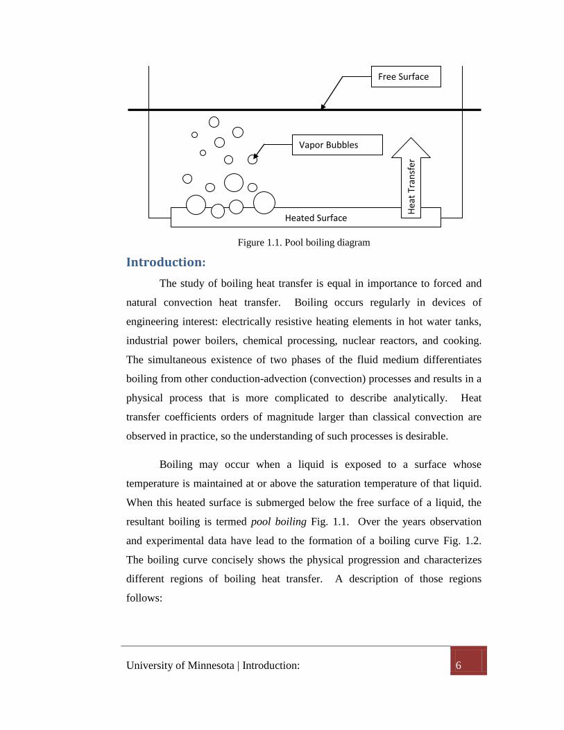
Figure 1.1. Pool boiling diagram

Introduction:

The study of boiling heat transfer is equal in importance to forced and

natural convection heat transfer. Boiling occurs regularly in devices of

engineering interest: electrically resistive heating elements in hot water tanks,

industrial power boilers, chemical processing, nuclear reactors, and cooking.

The simultaneous existence of two phases of the fluid medium differentiates

boiling from other conduction-advection (convection) processes and results in a

physical process that is more complicated to describe analytically. Heat

transfer coefficients orders of magnitude larger than classical convection are

observed in practice, so the understanding of such processes is desirable.

Boiling may occur when a liquid is exposed to a surface whose

temperature is maintained at or above the saturation temperature of that liquid.

When this heated surface is submerged below the free surface of a liquid, the

resultant boiling is termed pool boiling Fig. 1.1. Over the years observation

and experimental data have lead to the formation of a boiling curve Fig. 1.2.

The boiling curve concisely shows the physical progression and characterizes

different regions of boiling heat transfer. A description of those regions

follows:

Heated Surface

Hea

t Tr

ansf

er

Free Surface

Vapor Bubbles


Figure 1.2. Boiling heat transfer coefficient curve

I. Convection is dominant. The heated surface is not above the

saturation temperature of the liquid. Heat transfer here is

dominated by conduction and advection of the fluid whether

forced or free.

II. Nucleate boiling begins. Bubbles are observed on the heated

surface. Sites where bubbles form are termed nucleation sites.

In this region heat is conducted away from the bubbles rapidly

enough such that it causes them to condense in the liquid pool

and prevents them from rising to the free surface.

III. Nucleate boiling. Bubbles do not condense in the pool; they

have enough energy to rise to the free surface.

IV. A maximum heat transfer coefficient is reached before transition

to film boiling occurs. At this point a film of vapor is observed

to exist on the heated surface. There is a temperature gradient in

this vapor film which acts as a resistance to heat transfer, so the

heat transfer coefficient decreases. Region IV is an unstable

film boiling state where nucleate and film boiling can coexist.

Burnout

Temperature Excess

Convection Nucleate Film

I II III IV V VI


V. Stable film boiling. A further reduction in heat transfer

coefficient due to the thermal resistance of the vapor film.

VI. Radiation heat transfer becomes a more significant contributor to

the overall heat transfer process here. Heat transfer will increase

until the temperature of the heated surface exceeds its melting

temperature and burnout results.

A deviation from traditional boiling heat transfer results when one

wishes to boil a binary mixture of two immiscible fluids. In such a mixture if

one of the liquids forms a suspension of many small droplets it is termed an

emulsion. Therefore, an emulsion is characterized by its dispersed component

and its continuous component. Emulsions can either be dilute or strong. A

dilute emulsion is a characterized by having less than ~5% volume fraction of

the dispersed component in the mixture. An interesting heat transfer

phenomenon occurs when the dilute emulsion being studied has a dispersed

component with a boiling (saturation) temperature below that of the continuous

component; in such a scenario, the degree of superheat required to achieve

boiling of the mixture is much higher than the superheat required to boil only

the dispersed component. However, the superheat required to boil the mixture

is lower than that required to boil only the continuous component. If the

dispersed component has a saturation temperature greater than the continuous

component, the effect is the opposite. This behavior was first observed in the

1970’s (Mori, Inui, and Komotori, 1978) with a great deal of further study

carried out by Bulanov and coworkers (Bulanov and Gasanov, 2007, 2008).

All liquids have a critical heat flux (CHF) value, a point at which the

liquid will entirely transition from nucleate to film boiling and a sharp rise in

temperature on the heated surface is observed. Transition to film boiling can

cause issues in devices that rely on the high heat transfer coefficients of

nucleate boiling to keep the surface at or below a specific temperature. Such

devices of engineering interest are high heat flux electronics. The CHF can be


manipulated with emulsions. For this paper heat transfer characteristics of

dilute emulsions of FC-72 and pentane in water are used at volume fractions of

0.1% and 0.5% (i.e. a 0.5% emulsion is 5 mL of the dispersed component in

1000 mL of water).

Consider the physical reasoning for investigating emulsions and their

use in boiling heat transfer: with an emulsion of water and refrigerant, such as

FC-72 or pentane, one can realize the best heat transfer characteristics of both

fluids. Water has a large heat capacity, thermal conductivity, is readily

available, and is non-toxic. FC-72 and pentane have saturation temperatures

(56°C and 36°C, respectively) which are below that of water (100°C) at

atmospheric pressure. As heat is transferred from a hot immersed surface to the

emulsion the small FC-72 or pentane droplets boil, an action which stirs up the

water locally. The localized bulk motion of fluid readily transfers the thermal

energy of the dispersed droplet to the water, a process much quicker than

thermal diffusion.

How the droplets boil and the macroscopic mechanism by which the

boiling occurs is yet not well understood. It is known that the droplets in the

emulsion, once superheated, initially exist in a meta-stable state. The droplets

remain in a liquid phase despite being well above the saturation temperature of

the fluid. The meta-stable droplets would instantaneously boil if they were to

encounter some sort of disturbance such as a nucleation site or liquid-vapor

interface. Typically nucleation sites exist on the material in contact with the

fluid. Manufacturing imperfections and voids in the material act as sites for

initiation to transition the fluid from a liquid to vapor state. Most of the

droplets that are superheated, however, do not come into contact with

nucleation sites on the heated surface and are surrounded by the continuous

component of the emulsion. The droplets receive their thermal energy from the

thermal boundary layer of the heated surface. The droplets in the mixture

transition to a vapor state but they do so by spontaneous nucleation. How

University of Minnesota | Literature Review 10

spontaneous nucleation occurs and how it propagates between droplets is not

well understood.

The work done for this paper is a continuation of research performed by

Roesle (2010) at the University of Minnesota. His work focused on boiling of

the same refrigerants at various volume fractions of emulsions over a small,

heated copper wire. Roesle appears to be the first researcher to develop a

fundamental understanding of boiling heat transfer in emulsions both from a

numerical modeling and experimental standpoint. He developed and solved an

Euler-Euler numerical model for multi-phase flow of the emulsion. Roesle’s

numerical modeling was limited to the heat transfer regime where only the

dispersed component boiled. That is to say, the numerical model included

equations for only the liquid state of the continuous component, but it did

account for both liquid and vapor states of the dispersed component. By

separately solving the liquid to vapor transition process of the dispersed

component a closure model for the larger set of equations of the mixture was

developed (Roesle, 2010).

Roesle measured heat fluxes that fell within the range of his numerical

model as well as heat fluxes high enough to boil the continuous component of

the emulsion. Similar heat transfer ranges for the emulsions are studied here.

No effort is made to develop a numerical model for comparison of the results.

This study is entirely intended to add to the small, but expanding, experimental

database of heat transfer experiments boiling dilute emulsions.

Literature Review

Modeling a multiphase flow introduces analytical and computational

challenges. Most multiphase flow solutions have been approached numerical

by computational fluid dynamics (CFD). There are typically three approaches

to CFD when solving a multiphase flow: direct numerical simulation (DNS),


Euler-Euler, and Euler-Lagrange (Rusche, 2002). An excellent graphical and

narrative description of the different approaches is described by Roesle (2010).

In a dispersed, multiphase flow there are many surfaces to track, and, therefore,

DNS is almost always too computationally intensive for solving practical

engineering problems within a reasonable timeframe or with limited computing

resources. There exist modeling limitations and challenges for choosing an

Euler-Euler modeling approach to multiphase flow, all of which are discussed

extensively by Roesle (2010). A literature review of the computational

modeling of emulsions is not covered under the scope of this paper. However,

a discussion of some experimental studies and a basic theoretical model of the

boiling of dilute emulsions follow.

Various emulsion heat transfer studies have been performed over the

past few decades. To date the mechanism and modeling of heat transfer in

dilute emulsions is being studied, but certainly not as aggressively as other

areas of heat transfer. Therefore, the amount of data available for review is

limited, and the investigators in this field appear over and over again in the

literature. As such, many of the same works reviewed by Roesle apply to this

study and the information presented here is an abbreviated summary of the

more in-depth review covered in Roesle’s paper.

Early studies of emulsions were carried out by Mori, Inui, and Komotori

(1978). These studies looked at oil in water emulsions with water

concentrations of 10 to 95%. At these concentrations the emulsions are not

considered dilute. Oil is the high boiling point liquid and was used with

emulsifiers to create stable emulsions. The heat transfer coefficients of the

emulsions were better or worse depending on the concentration of the emulsion.

The type of oil used had little effect. Most notable was the observation that high

amounts of superheat were needed to boil the dispersed water component.

Spontaneous nucleation was required to boil the droplets since the water was

not usually in direct contact with the heated surface.


Figure 2.1. Pool boiling heat transfer coefficients for pure liquids and emulsions: (1)

water, (2) R-113, (3) PES-5, (4) water in PES-5 emulsion, (5) R-113 in

water emulsion (Bulanov, 2006).

Although Mori et al. studied strong emulsions, there are, of course, a

number of dilute emulsion studies which are more relevant to this paper. Early

studies by Bulanov and co-workers noticed favorable characteristics of dilute

emulsions (Bulanov, Skripov, and Khmyl’nin, 1984; Bulanov, Gasanov, and

Turchaninova, 2006). They find that a high degree of superheat is required to

boil the dispersed component, but that heat transfer coefficients were always

higher than with just the continuous component. Figure 2.1 shows the results of

Bulanov et. al (2006) in which the heat transfer coefficients of pure water, R-

113, PES-5, and emulsions of R-113 and PES-5 in water are recorded. Bulanov

et. al focused on using emulsions as a means to prevent the transition to film

boiling of a liquid and thus prevent burnout of the heated surface. A thin,

vertical platinum wire was used in the experiments. Figure 2.2 shows a

schematic of the apparatus used in the experiment.


Figure 2.2. Schematic of the experimental setup: (1) thermostat, (2) glass cylinder, (3)

platinum wire, (4) resistance box, (5) electric current source, (6) digital

voltmeters, (7) potential leads, (8) reference resistance coil, (9)

thermocouple (Bulanov, 2006).

Nucleate boiling was observed without transition to film boiling.

Bulanov et al. also investigated the effect of droplet size and found that the

degree of superheat required for boiling to initiate decreased with increasing

droplet size, but once initiated the heat transfer coefficient had little dependence

on the droplet size (Bulanov, Skripov, Gasanov, and Baidakov; 1996).

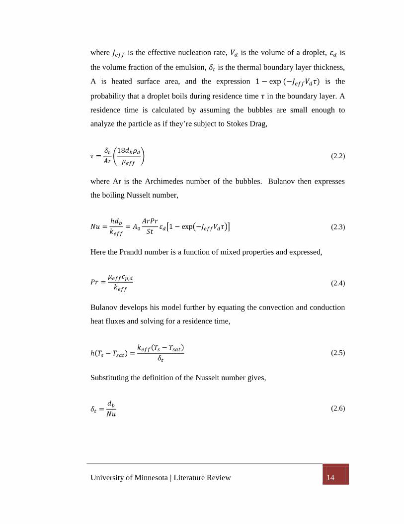
Bulanov (2001) developed a simplified model of boiling dilute

emulsions based on experimental results. He assumes that each emulsion

droplet boils randomly inside the thermal boundary layer, so boiling does not

depend on contact with the heated surface. He assumes that the temperature

profile of the boundary layer is linear, for purposes of calculating its thickness;

however, for purposes of calculating the nucleation rate, he assumes the

temperature is uniform. The energy to boil a droplet comes from the

surrounding fluid in the boundary layer which decreases the temperature of the

boundary layer directly surrounding a droplet. He modeled the heat transfer to

a droplet as,

(2.1)


where is the effective nucleation rate, is the volume of a droplet, is

the volume fraction of the emulsion, is the thermal boundary layer thickness,

A is heated surface area, and the expression is the

probability that a droplet boils during residence time in the boundary layer. A

residence time is calculated by assuming the bubbles are small enough to

analyze the particle as if they’re subject to Stokes Drag,

(2.2)

where Ar is the Archimedes number of the bubbles. Bulanov then expresses

the boiling Nusselt number,

(2.3)

Here the Prandtl number is a function of mixed properties and expressed,

(2.4)

Bulanov develops his model further by equating the convection and conduction

heat fluxes and solving for a residence time,

(2.5)

Substituting the definition of the Nusselt number gives,

(2.6)

University of Minnesota | Experimental Apparatus and Design: 15

Figure 2.3. Nucleation rate J: (1) pure water, emulsified droplets of

(2) R-113, (3) water, (4) pentane, and (5) ethanol. (Bulanov and

Gasanov, 2008).

Bulanov then iteratively solves Eq. (2.2), Eq. (2.6) and Eq. (2.3) for the boiling

heat transfer coefficient. The model developed is not used to predict heat

transfer coefficient rates but to determine experimentally. is

typically found to have a single value for a set of experimental data, but

varies with temperature and other parameters Fig. 2.3.

Bulanov’s model, matched with experimental results, shows that the

nucleation rate for an emulsified liquid is much higher than for pure liquid of

the continuous component. Although the model was developed assuming

spontaneous nucleation as the reason for the superheated droplets boiling, there

are other mechanisms responsible still awaiting discovery.

Experimental Apparatus and Design:

The apparatus used for these experiments is the same used by Roesle

(2010). The apparatus consists of a container to hold the emulsion and a bus-


bar assembly Fig. 3.1 that holds the heated material below the free surface of

the pool. There are two 0.25 in. square copper rods that extend below the

surface of the pool; these rods supply power to the strip or wire under study.

Figure 3.1. (Left) Pool container, (Right) bus-bar assembly

There are two wire leads that are in constant contact with the heated

wire, and they measure voltage across the wire during the experiment Fig. 3.3.

Voltage is not measured through the bus bars. By not measuring the voltage

through the bus bars the error associated with measuring the power dissipation

of the bars and the resistance of the connection between the strip and the bars as

sources of voltage drop is eliminated. A potentiometer controls power through

two parallel transistors that supply power to the heated strip. There is a low-

ohm, high-tolerance resistor in series with the heated strip, across which are

another pair of leads, which measure the known resistor’s voltage drop. See

Appendix A for a complete circuit diagram of the apparatus.


Figure 3.2. Apparatus assembly

By measuring the voltage across the known resistance, Ohm’s law Eq. (3.1) can be

used to obtain the current through the strip,

(3.1)

With the current known the voltage across the heated strip can be used

to calculate the power being dissipated by the strip,

(3.2)


Combining with Eq. (3.1),

(3.3)

In Roesle’s experiment a 101 μm diameter (38 AWG) round copper

wire was submerged in a pool of emulsion. In the present study a steel strip is

submerged to observe the heat transfer differences in the emulsion on a flat

surface versus a horizontal cylinder. A 300W power supply is used to heat the

strip, and the strip is made of 1008 steel which has a very similar thermal

coefficient of resistivity (TCR) to copper. The Thermal Coefficient of

Resistivity is a measure of how much the resistivity of a material changes with

temperature. Resistivity is simply the electrical resistance of a material that is

independent of geometry. The resistivity is defined,

(3.4)

Although the resistivity of a material does not depend on geometry it is

a function of temperature, and the TCR is the slope of such a function. The

TCR is roughly linear over a range of temperatures for many materials. In this

experiment, the TCR is used to calculate the surface temperature of the metal

strip. The TCR is defined,

(3.5)

Table 3.1 shows a comparison between the TCR of copper, 1008 steel, and a

variety of stainless which was another option for the experiment. Table 3.1

shows that 1008 steel is the preferred choice of materials because its average

TCR is roughly identical over a similar range of temperatures when compared

with copper. By contrast 304 stainless differs by nearly 76.3%.


Figure 3.3 Heated strip detail

Table 3.1. Thermal coefficient of resistivity comparison

Pure Copper

Smithells Metals Reference Book (8th ed) - Sec 19.1

Temp [C] Electrical Resistivity [Ohm-cm] TCR [1/K]

20 1.673E-06

27 1.725E-06 4.440E-03

127 2.402E-06 3.925E-03

Average -> 3.925E-03

1008 Steel

Smithells Metals Reference Book (8th ed) - Sec 14.11

AISI 1008 Steel Annealed


27 1.470E-05 <-Measured

100 1.900E-05 4.007E-03

200 2.630E-05 3.842E-03


Difference From Cu -> 0.0%

301/302/304 Stainless Steel

www.matweb.com

ASTM A 666 Type 302


0 7.200E-05

100 7.820E-05 8.611E-04

200 8.600E-05 9.974E-04


Difference From Cu -> 76.3%

Heated Strip

Bus Bars

Voltage Sense Leads

Acrylic Guides


In reality other types of steel meet the above criteria; however, 1008

steel was chosen because it is readily available, common in a range of thin sheet

stock, and is easy to work with. It also has a resistivity that is 10 times greater

than copper. The geometry of the strip can also be easily manufactured with a

large enough surface area without having to use an aggressively sized power

supply.

Figure 3.4. Heated strip in pool of emulsion

The power supply being used grants a maximum of 30A at 9VDC as

advertised which should deliver 270W at maximum output. Roesle was able to

obtain around 240W at 28.7A and 8.5VDC. To achieve the highest heat fluxes

possible utilizing the same power supply, it is desirable to match the resistance

of the copper wire at the temperature where the highest power draw on the

power supply was observed. In Roesle’s experiments 240W of dissipation was

observed at a wire temperature of 127°C. If a strip with too low of a resistance

is used, then the power supply is current limited at 30A. If the resistance is too


high, then it is voltage limited at 9 VDC. If either of these conditions occurs,

the power supply will not be used effectively and a lower than desired power

dissipation will result. Using Ohm’s law, it can be shown that Roesle observed

a resistance of 0.3 Ω at 127°C. Rearranging Eq. (3.5) gives,

(3.6)

Table 3.1 gives the following properties for 1008 steel,

(3.7)

(3.8)

Plugging the above values into Eq. (3.6) gives,

(3.9)

Rearranging Eq. (3.4),

(3.10)

where L is the distance between the bus bars (10 cm in the apparatus). The

cross-sectional area required is then,

(3.11)

Table 3.2 shows a few combinations of thicknesses and widths that meet the

cross-sectional area criteria.


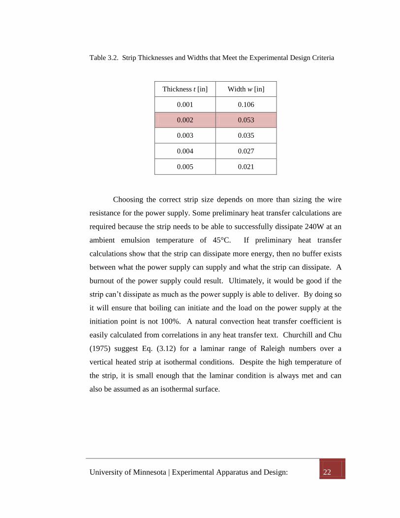
Table 3.2. Strip Thicknesses and Widths that Meet the Experimental Design Criteria

Thickness t [in] Width w [in]

0.001 0.106

0.002 0.053

0.003 0.035

0.004 0.027

0.005 0.021

Choosing the correct strip size depends on more than sizing the wire

resistance for the power supply. Some preliminary heat transfer calculations are

required because the strip needs to be able to successfully dissipate 240W at an

ambient emulsion temperature of 45°C. If preliminary heat transfer

calculations show that the strip can dissipate more energy, then no buffer exists

between what the power supply can supply and what the strip can dissipate. A

burnout of the power supply could result. Ultimately, it would be good if the

strip can’t dissipate as much as the power supply is able to deliver. By doing so

it will ensure that boiling can initiate and the load on the power supply at the

initiation point is not 100%. A natural convection heat transfer coefficient is

easily calculated from correlations in any heat transfer text. Churchill and Chu

(1975) suggest Eq. (3.12) for a laminar range of Raleigh numbers over a

vertical heated strip at isothermal conditions. Despite the high temperature of

the strip, it is small enough that the laminar condition is always met and can

also be assumed as an isothermal surface.


(3.12)

The Prandtl and Raleigh numbers are evaluated at a film temperature which is

defined,

(3.13)

The average Nusselt number is defined,

(3.14)

Table 3.3 shows the predicted power dissipation and average heat

transfer coefficients for four different strip widths. Power dissipations of 135.4

W and 81.5 W are predicted for strip widths of 0.103 in. and 0.053 in.,

respectively. This is good, because it is known that with the resistance of the

strip at 127°C the power supply is capable of nearly 240 W. At this point any

of strip width meets the need of the experiment.

Figure 3.5. Strip geometry

Width

Thickness


Table 3.3. Strip heat transfer calculations

Length [cm] = 10 Bulk Temperature [C] = 45 Strip Temperature [C] = 127

Thickness [inch] = 0.001

Thickness [inch] = 0.002 Width [inch] = 0.106

Width [inch] = 0.053

Ra # [] = 210,219

Ra # [] = 26,277

Nu_avg # [] = 12.28

Nu_avg # [] = 7.40 h_avg [W/m^2-C] = 3065

h_avg [W/m^2-C] = 3691

Surface Area [m^2] = 5.386E-04

Surface Area [m^2] = 2.693E-04 Power Dissipation [W] = 135.4

Power Dissipation [W] = 81.5

Heat Flux [W/m^2] = 2.51E+05

Heat Flux [W/m^2] = 3.03E+05

Thickness [inch] = 0.003

Thickness [inch] = 0.004 Width [inch] = 0.035

Width [inch] = 0.027

Ra # [] = 7,786

Ra # [] = 3,285

Nu_avg # [] = 5.63

Nu_avg # [] = 4.69 h_avg [W/m^2-C] = 4212

h_avg [W/m^2-C] = 4677





Heat Flux [W/m^2] = 3.45E+05

Heat Flux [W/m^2] = 3.84E+05

A strip at a width of 0.053 in. and thickness of 0.002 in. was chosen for

the following reasons: the width associated with the 0.002 in. thickness will

give a larger heat flux than the 0.001 in. shim stock but still maintains a high

width to thickness ratio. If the width to thickness ratio gets too small, then the

strip will begin to act like a heated bar rather than a flat plate. Furthermore, the

thermal and hydrodynamic boundary layers will not develop in the same way,

and leading and trailing edge effects of fluid flow could be greatly influential

on the heat transfer results. Furthermore, 0.002 in. shim stock is easy to work

with without being flimsy, and small metal shears exist to be able to cut the

material to the desired width very precisely while maintaining a clean leading

University of Minnesota | Data Reduction: 25

edge. There were complications cutting 0.003 in. and 0.004 in. shim stock to

widths of 0.035 in. and 0.027 in., respectively, because the strips would curl

while being sheared. The curling gave a very unclean leading edge of the strip.

The resistance of the strip needs to be accurately checked at a known

temperature before each experimental run. Measuring the resistance is

accomplished by attaching a strip to the apparatus and submerging it in a pool

of emulsions before each trial run. The emulsion temperature was measured

with a thermocouple tree containing four Type E thermocouples. The strip was

allowed to equilibrate to the temperature of the pool, and the resistance was

then measured with an accurate four-wire resistance method. The distance

between the strip voltage leads was measured using a dial calipers to within a

conservative uncertainty of in. The expected resistance measured at

27°C is approximately,

(3.15)

Data Reduction:

An Agilent 34970A DAQ system was used to record data for the

experiment. Data is recorded at a frequency of once per second. The DAQ

card has a multiplexer, which isolates thermocouple readings from other

voltage noise, allowing for a true differential reading of the voltage across the

thermocouple. The voltage sense leads, Fig. 3.3, measure the voltage drop

across the strip and the total resistance of the strip can be reduced from its

reading. However, a temperature variation may exist in the strip because of the

large bus bars on either side of it. The bus bars act as heat sink and hold the

two ends of the strip at roughly the temperature of the pool, . The resistance

that is measured by the DAQ is therefore a summation of small segments of the


Figure 3.6. Apparatus strip detail

wire at different temperatures and different resistances. Deducing the proper

strip temperature can be approximately corrected for by considering a fin

analysis of the strip. Figure 3.6 shows the geometry and the coordinate system

for the fin analysis problem.

By defining the boundary conditions of the differential

equation becomes homogenous and easier to solve. The fundamental equation

of the problem can be formulated by considering a differential element of the

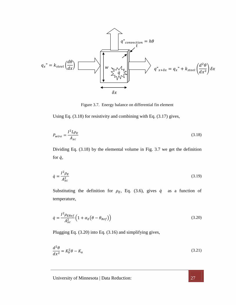
strip. Figure 3.7 shows a one-dimensional differential element of the strip with

the energy inflows and outflows. The differential equation is,

(3.16)

Where is the volumetric heat generation rate. There exists a dependence of

on resistance, which varies with temperature, but the electrical current is the

same throughout the entire strip. The power dissipation of the wire is,

(3.17)

X

Voltage Sense

Wires

Bus Bars

Heated Strip

L


Figure 3.7. Energy balance on differential fin element

Using Eq. (3.18) for resistivity and combining with Eq. (3.17) gives,

(3.18)

Dividing Eq. (3.18) by the elemental volume in Fig. 3.7 we get the definition

for ,

(3.19)

Substituting the definition for , Eq. (3.6), gives as a function of

temperature,

(3.20)

Plugging Eq. (3.20) into Eq. (3.16) and simplifying gives,

(3.21)


where the constants are defined,

(3.22)

(3.23)

The solution to the differential equation is a superposition of the homogenous

and non-homogenous solutions, Eq. (3.24) and Eq. (3.25) respectively,

(3.24)

(3.25)

The solution to Eq. (3.21) is,

(3.26)

There are two boundary conditions at, and

, Fig. 3.6. The

constants and can be solved for by applying boundary conditions to Eq.

(3.26) and yield the final solution to the differential equation,

(3.27)

For most of the conditions in the experiment is large; therefore, the

denominator of the hyperbolic cosine function is typically much greater than

the numerator. Therefore, the wire has a mostly uniform temperature, and only

near the ends does the temperature differ much from the centerline temperature

of the strip.


The centerline temperature of the strip is designated,

(3.28)

Because of the temperature variation in the strip, the resistance varies also. The

resistance of the strip is,

(3.29)

Combining Eq. (3.6) with Eq. (3.29) gives,

(3.30)

Using the definition ,

(3.31)

The solution for Eq. (3.26) can be combined with Eq. (3.31),

(3.32)


and integrated to yield,

(3.33)

where is defined,

(3.34)

Because is large for these experiments,

, and Eq. (3.33) can

be rewritten,

(3.35)

Now using Eq. (3.5) an expression for wire temperature can be established,

(3.36)

Equation (3.36) can be combined with Eq. (3.1) to get an expression for wire

temperature in terms of measured values,

(3.37)

University of Minnesota | Uncertainty analysis and calibration: 31

To get an expression for the temperature at the centerline of the wire Eq. (3.35)

can be combined with Eq. (3.36),

(3.38)

Away from the bus bars and close to the middle of the wire, heat conduction

along the longitudinal axis of the wire is very small, so the local, centerline heat

flux can be defined,

(3.39)

and the heat transfer coefficient at the midpoint can be defined,

(3.40)

Uncertainty analysis and calibration:

Because the equipment and data acquisition are the same used by Roesle

(2010), the same type of uncertainty analysis of the results applies. As noted by

Roesle, under most circumstances the uncertainty of Eq. (3.38) is largely a

result of the assumptions used to develop it and not a result of the accuracy of

the measurements. The two grandest assumptions are: the heat transfer

coefficient is constant along the entire strip and that the conduction equation is

one-dimensional. Under most circumstances, the temperature of the wire is

measured to within an uncertainty of approximately ± 2°C. The uncertainty in

the wire temperature becomes significantly larger at low current. The

uncertainty in the heat transfer coefficient is also small except at low power.

University of Minnesota | Results and Discussion: 32

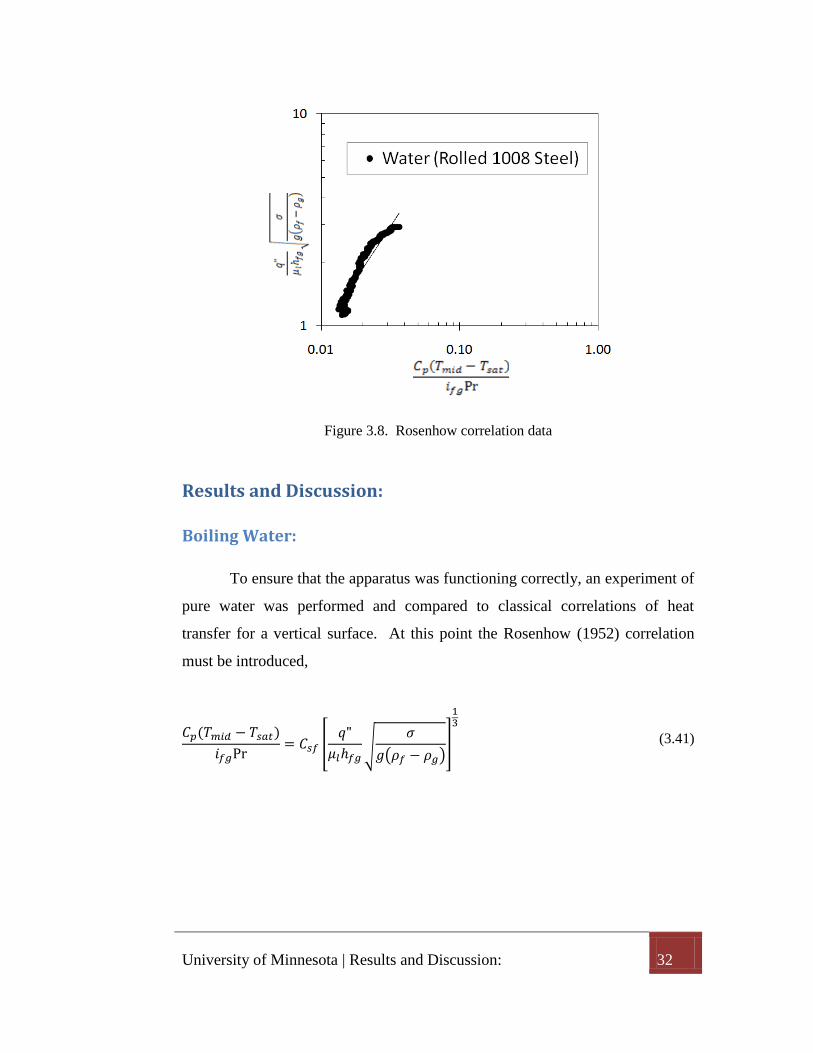
Figure 3.8. Rosenhow correlation data

Results and Discussion:

Boiling Water:

To ensure that the apparatus was functioning correctly, an experiment of

pure water was performed and compared to classical correlations of heat

transfer for a vertical surface. At this point the Rosenhow (1952) correlation

must be introduced,

(3.41)


Eq. (3.41) is a correlation from experimental data of nucleate pool

boiling. The empirical constant varies with the type and surface

preparation of the material under study. A constant for rolled 1008 steel could

not be found in the literature, so a constant was evaluated from this paper’s

experimental results. Figure 3.8 shows the correlation of the pool boiling data;

the empirical constant is determined to be to best fit the data.

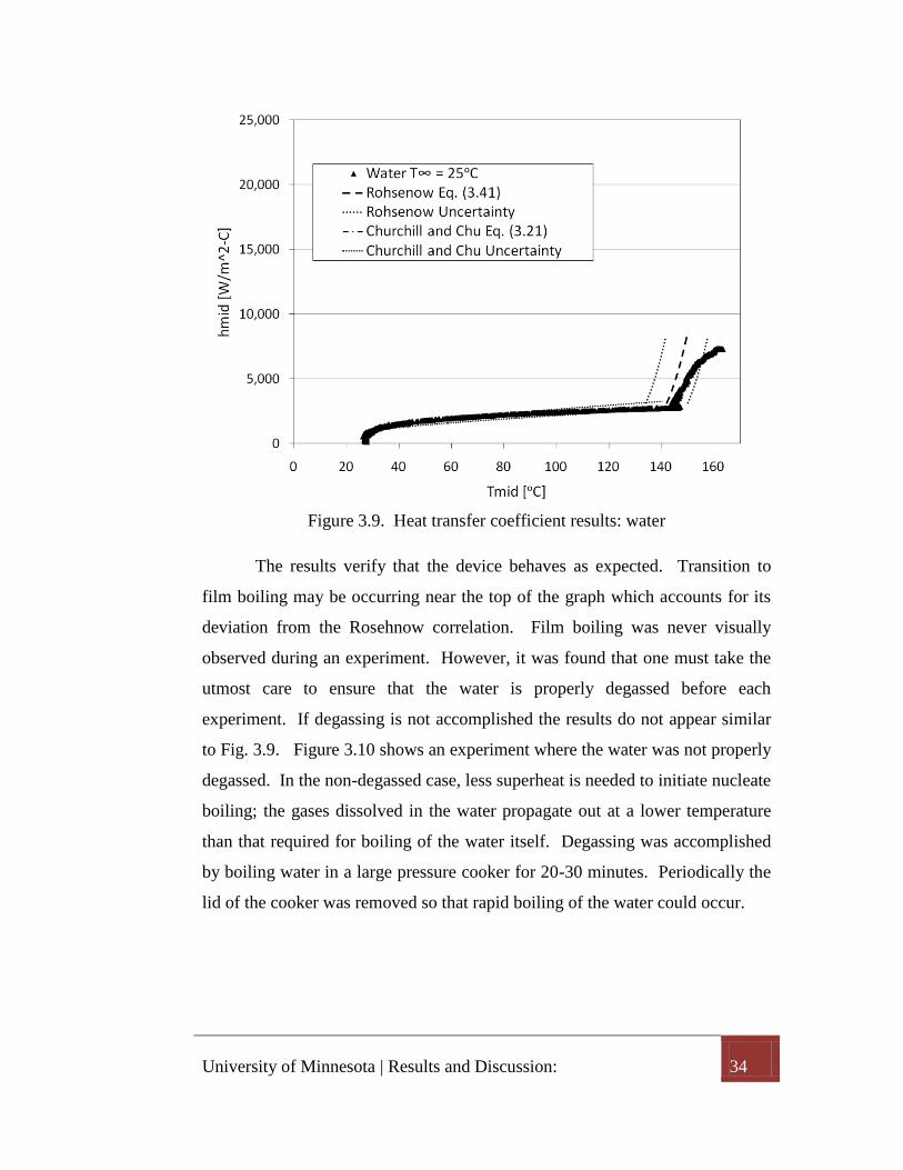
Figure 3.9 shows the heat transfer results for pure water. There are a number of

interesting things to notice. The amount of superheat needed to initiate boiling

is large, boiling does not actually occur until the heated surface temperature

reaches nearly 150°C. Churchill and Chu (1975) present an average Nusselt

number Eq. (3.12) relation for natural convection on a vertical isothermal

surface and it is found to agree very well with the data. The uncertainty of the

correlations by Churchill and Chu are assumed to be around 10%. For

saturated boiling Eq. (3.41) typically has ~25% error in

(Lienhard and Lienhard, 2008). Both of the uncertainty lines are graphed with

the data, and most of the data is found to correlate well in the boiling and

natural convection regimes.


Figure 3.9. Heat transfer coefficient results: water

The results verify that the device behaves as expected. Transition to

film boiling may be occurring near the top of the graph which accounts for its

deviation from the Rosehnow correlation. Film boiling was never visually

observed during an experiment. However, it was found that one must take the

utmost care to ensure that the water is properly degassed before each

experiment. If degassing is not accomplished the results do not appear similar

to Fig. 3.9. Figure 3.10 shows an experiment where the water was not properly

degassed. In the non-degassed case, less superheat is needed to initiate nucleate

boiling; the gases dissolved in the water propagate out at a lower temperature

than that required for boiling of the water itself. Degassing was accomplished

by boiling water in a large pressure cooker for 20-30 minutes. Periodically the

lid of the cooker was removed so that rapid boiling of the water could occur.


Figure 3.10. Heat transfer coefficient results: water (not degassed)

Figure 3.11. Bubbles on heated strip

Figure 3.11 shows what the heated strip looks like once boiling has

initiated over the entire heated surface. As expected a large jump in the heat

transfer coefficient is observed when boiling initiates. The bubbles that initially

appear on the surface do not grow, detach, and rise to the surface until a higher

heat flux is reached at approximately 0.5 MW/m^2. Roesle noticed a vibration

of his heated wire during some of his experiments, which he theorizes is due to


the rapid generation and release of bubbles from the surface. No vibration of

the strip was observed during any of these experiments. Likely, no vibration

exists due to the substantial size of the surface, so the generation and release of

bubbles has a very minimal forcing effect on the strip.

FC-72 in Water Emulsion

Figure 3.12. Heat transfer coefficient results: 0.5% FC-72 in water

Figure 3.12 and Fig. 3.13 show the results of an emulsion of 0.5% and

0.1% FC-72, respectively, in water at a bulk temperature of 25°C. The amount

of superheat required for boiling of the mixture was reduced compared to the

pure water case. There exist many similarities in trends between Roesle’s

experiments and these. The natural convection heat transfer coefficient is

actually slightly reduced for the emulsions compared to that of pure water, but

there is an increase in the boiling heat transfer coefficient for each of the

emulsions. The temperature drop after the initiation of boiling for pure water

occurs immediately and then the wire temperature continues to rise


Figure 3.13. Heat transfer coefficient results: 0.1% FC-72 in water

with increasing heat flux. For all of the emulsions the drop in surface

temperature is gradual with increasing heat flux. Roesle noticed a plateauing of

the boiling heat transfer coefficient possibly due to the critical heat flux being

reached. A similar plateauing effect is observed for these experiments, and is

very pronounced for the 0.1% FC-72 case; this could be a result of film boiling.

However, a film of vapor was never observed on the strip. Because the 0.1%

FC-72 emulsion does not reduce the boiling saturation temperature much, what

is likely happening is the continuous component is participating in the boiling

process at the top of the data. At 160°C surface temperature the difference in

the heat transfer coefficient between the pure water case and the 0.1% FC-72

case is approximately 1.4%. Roesle found the results for the 0.1% FC-72

volume fraction to be anomalous as well.


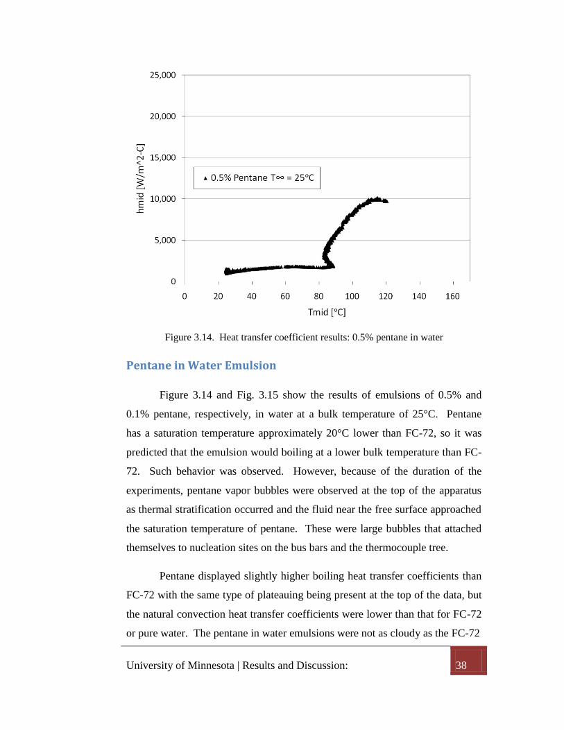
Figure 3.14. Heat transfer coefficient results: 0.5% pentane in water

Pentane in Water Emulsion

Figure 3.14 and Fig. 3.15 show the results of emulsions of 0.5% and

0.1% pentane, respectively, in water at a bulk temperature of 25°C. Pentane

has a saturation temperature approximately 20°C lower than FC-72, so it was

predicted that the emulsion would boiling at a lower bulk temperature than FC-

72. Such behavior was observed. However, because of the duration of the

experiments, pentane vapor bubbles were observed at the top of the apparatus

as thermal stratification occurred and the fluid near the free surface approached

the saturation temperature of pentane. These were large bubbles that attached

themselves to nucleation sites on the bus bars and the thermocouple tree.

Pentane displayed slightly higher boiling heat transfer coefficients than

FC-72 with the same type of plateauing being present at the top of the data, but

the natural convection heat transfer coefficients were lower than that for FC-72

or pure water. The pentane in water emulsions were not as cloudy as the FC-72


Figure 3.15. Heat transfer coefficient results: 0.1% pentane in water

in water emulsions. Because pentane is less dense than water, the emulsion

droplets tended to rise to the free surface during the experiments. This type of

behavior was exacerbated by the buoyancy of the heated fluid around the strip

rising to the surface and remaining there (thermal stratification in the

apparatus). This caused what appeared to be a higher concentration of

emulsion droplets near the top of the apparatus by the end of the experiment.

Because FC-72 is more dense than water these two effects counteracted each

other: the heated fluid would bring emulsions to the top of the pool and then the

emulsion droplets would gradually fall down keeping the entire mixture

relatively well distributed.

It may be of interest to note that each time the strip was removed from

the pool it was effectively wetted with the dispersed component of the

emulsion. Strip wetting was observed for both the FC-72 and pentane

emulsions. Roesle (2010) notes that the decrease in natural convection heat

transfer coefficients should not be present at lower volume fractions, such as

University of Minnesota | Final Remarks: 40

0.1%. The decrease in the average thermal conductivity and viscosity are very

minimal at such a low volume fraction. He theorizes that the decrease in heat

transfer may be due to the observed wetted layer of the low saturation

temperature liquid on the strip. Pentane and FC-72 have conductivities much

lower than that of water (at 25 °C, k = 0.595, 0.117, and 0.056 W/m-°C for

water, pentane, and FC-72 respectively). However, it is impossible to

determine whether the strip is thoroughly wetted (visually or by instrument

measurement) by the dispersed component when the apparatus is submerged in

the pool.

Final Remarks:

Deviation from Roesle’s experiments

Roesle carried out experiments at bulk temperatures of 25 and 44 °C.

The largest deviation in process from Roesle’s experiments is that in this study

the bulk temperature was monitored throughout the experiment and the heat

transfer coefficients calculated were based off a measured instead of the

initial temperature of the fluid and temperature of the heated surface. Because

of the small size of the pool, the temperature of the liquid was found to rise as

much as 6 °C between the beginning and end of the experiments. Experiments

only take a few minutes to complete.

Future work:

It was observed that natural convection heat transfer coefficients were

reduced with dilute emulsions. Investigation into the reasoning behind the

reduction in heat transfer coefficients is merited. Numerical modeling of the

heat transfer from a heated strip was never completed and could be

advantageous for a comparison of the results. Furthermore, additional

experiments using different emulsions, emulsion bulk temperatures, and

material type and geometry should be carried out.

University of Minnesota | Final Remarks: 41

Conclusion

Boiling heat transfer experiments of FC-72 and pentane emulsions in

water were completed. A 1008 steel strip was submerged in a pool of dilute

emulsion and heated with a 270W power supply. The initial bulk temperature of

the emulsion before the start of the experiment was approximately 25°C. Heat

transfer coefficient improvements were realized in the nucleated boiling heat

transfer regime, but natural convection coefficients were reduced slightly. The

onset of film boiling was never observed. Boiling initiated at lower surface

temperatures than that required for boiling of the continuous component of the

emulsion. The enhancement in the heat transfer coefficients could be

manipulated by varying the volume fraction of the emulsions to achieve a

desired mixture boiling temperature. The type of heat transfer enhancement

documented here could prove advantageous in the cooling of high heat flux

electronics where one wishes to maintain the surface at as low a temperature as

possible while maintaining a high critical heat flux.

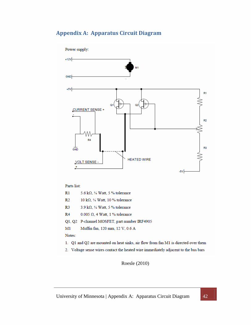
University of Minnesota | Appendix A: Apparatus Circuit Diagram 42

Appendix A: Apparatus Circuit Diagram

Roesle (2010)

University of Minnesota | Works Cited: 43

Works Cited:

Arpaci, V. S. (1991). Conduction Heat Transfer (Abridged ed.). Boston, MN:

Pearson Custom Publishing.

Bulanov, N. V., Skripov, V. P., and Khmyl’nin, V. A. (1984), “Heat transfer to

emulsion with superheating of its disperse phase,” Journal of Engineering

Physics, 46(1), pp. 1-3.

Bulanov, N. V., Gasanov, B. M., and Turchaninova, E. A. (2006), “Results of

experimental investigation of heat transfer with emulsions with low-boiling

disperse phase,” High Temperature, 44(2), pp. 267-282.

Bulanov, N. V. and Gasanov, B. M. (2007), “Special features of boiling of

emulsions with a low-boiling dispersed phase,” Heat Transfer Research, 38(3),

pp. 259-273.

Bulanov, N. V. and Gasanov, B. M. (2008), “Peculiarities of boiling of

emulsions with a low-boiling disperse phase,” International Journal of Heat

and Mass Transfer, 51, pp. 1628-1632.

Roesle, M. L. (2010). “Boiling of Dilute Emulsions,” Ph.D. Thesis, University

of Minnesota, Minneapolis, MN.

Churchill, S. W., and H. H. S. Chu. (1975) “Correlating Equations for Laminar

and Turbulent Free Convection from a Vertical Plate,” Int. J. Heat Mass

Transfer, vol. 18, pp. 1323

Gale, W.F.; Totemeier, T.C. (2004). Smithells Metals Reference Book (8th

Edition). Elsevier. pp. 14.1-45

Holman, J. P. (2002). Heat Transfer (9th

ed.). New York, NY: McGraw-Hill.

Lienhard, J. H. IV and Lienhard, J. H. V (2008), A Heat Transfer Textbook, 4th

Ed., Cambridge, MA: Phlogiston Press. Online version 2.01 retrieved April

25th, 2011 from http://web.mit.edu/lienhard/www/ahtt.html.

Matweb

Mori, Y. H., Inui, E., and Komotori, K. (1978), “Pool boiling heat transfer to

emulsions,” Transactions of the ASME Journal of Heat Transfer, 100(4), pp.

613-617.

Oberg, E.; Jones, F. D.; Horton, H. L.; Ryffel, H. H. (2008). Machinery's

Handbook (28th ed.). Industrial Press. pp. 402

University of Minnesota | Works Cited: 44

Rusche, H. (2002), “Computation fluid dynamics of dispersed two-phase flows

at high phase fractions,” Ph.D. Thesis, University of London, London.

Rohsenow, W. M., and P. Griffith. (1955) “Correlation of Maximum Heat Flux

Data for Boiling of Saturated Liquids,” AIChE-ASME Heat Transfer Symp.,

Louisville, Ky.

boiling dilute emulsions on a heated striplunde189/documents/davidlunde_boiling...boiling water:...

Documents