Doctoral Thesis, Periodical Part, Published Version

Bode, FelixEarly-Warning Monitoring Systems for Improved DrinkingWater Resource ProtectionMitteilungen. Institut fĂ¼r Wasser- und Umweltsystemmodellierung, Universität Stuttgart

Zur Verfügung gestellt in Kooperation mit/Provided in Cooperation with:Universität Stuttgart

Verfügbar unter/Available at: https://hdl.handle.net/20.500.11970/106485

Vorgeschlagene Zitierweise/Suggested citation:Bode, Felix (2018): Early-Warning Monitoring Systems for Improved Drinking WaterResource Protection. Stuttgart: Universität Stuttgart, Institut fĂ¼r Wasser- undUmweltsystemmodellierung (Mitteilungen. Institut fĂ¼r Wasser- undUmweltsystemmodellierung, Universität Stuttgart, 261).http://dx.doi.org/10.18419/opus-10268.

Standardnutzungsbedingungen/Terms of Use:

Die Dokumente in HENRY stehen unter der Creative Commons Lizenz CC BY 4.0, sofern keine abweichendenNutzungsbedingungen getroffen wurden. Damit ist sowohl die kommerzielle Nutzung als auch das Teilen, dieWeiterbearbeitung und Speicherung erlaubt. Das Verwenden und das Bearbeiten stehen unter der Bedingung derNamensnennung. Im Einzelfall kann eine restriktivere Lizenz gelten; dann gelten abweichend von den obigenNutzungsbedingungen die in der dort genannten Lizenz gewährten Nutzungsrechte.

Documents in HENRY are made available under the Creative Commons License CC BY 4.0, if no other license isapplicable. Under CC BY 4.0 commercial use and sharing, remixing, transforming, and building upon the materialof the work is permitted. In some cases a different, more restrictive license may apply; if applicable the terms ofthe restrictive license will be binding.

Heft 261 Felix Bode

Early-Warning Monitoring Systems for Improved Drinking Water Resource Protection

Early-Warning Monitoring Systems for Improved Drinking Water Resource Protection

Von der Fakultät Bau- und Umweltingenieurwissenschaften der Universität Stuttgart zur Erlangung der Würde eines Doktor-Ingenieurs (Dr.-Ing.) genehmigte Abhandlung

Vorgelegt von Felix Bode

aus Diepholz

Hauptberichter: Prof. Dr.-Ing. Wolfgang Nowak

Mitberichter: Prof. Dr. rer. nat. Dr.-Ing. András Bárdossy

Mitberichter: Prof. Dr. Patrick M. Reed

Tag der mündlichen Prüfung: 17. September 2018

Institut für Wasser- und Umweltsystemmodellierung der Universität Stuttgart

2018

Heft 261 Early-Warning Monitoring Systems for Improved Drinking Water Resource Protection

von Dr.-Ing. Felix Bode

Eigenverlag des Instituts für Wasser- und Umweltsystemmodellierung der Universität Stuttgart

D93 Early-Warning Monitoring Systems for Improved Drinking Water Resource Protection

Bibliografische Information der Deutschen Nationalbibliothek Die Deutsche Nationalbibliothek verzeichnet diese Publikation in der Deutschen Nationalbibliografie; detaillierte bibliografische Daten sind im Internet über http://www.d-nb.de abrufbar

Bode, Felix: Early-Warning Monitoring Systems for Improved Drinking Water Resource

Protection, Universität Stuttgart. - Stuttgart: Institut für Wasser- und Umweltsystemmodellierung, 2018

(Mitteilungen Institut für Wasser- und Umweltsystemmodellierung, Universität

Stuttgart: H. 261) Zugl.: Stuttgart, Univ., Diss., 2018 ISBN 978-3-942036-65-8 NE: Institut für Wasser- und Umweltsystemmodellierung <Stuttgart>: Mitteilungen

Gegen Vervielfältigung und Übersetzung bestehen keine Einwände, es wird lediglich um Quellenangabe gebeten. Herausgegeben 2018 vom Eigenverlag des Instituts für Wasser- und Umweltsystem-modellierung

Druck: DCC Kästl e.K., Ostfildern

Danksagung

Ein herzliches Dankeschön geht an meinen Betreuer und Hauptberichter WolfgangNowak, der mich jederzeit gefördert und unterstützt hat. Außerdem möchte ich michbei András Bárdossy und Patrick Reed für ihren Mitbericht bedanken. Ein besondererDank geht hierbei an Patrick Reed, der mich für drei Monate in seiner Arbeitsgruppean der Cornell University in Ithaca aufgenommen hat.

Ein großer Dank geht auch an die gesamte Gruppe des LS3, die jederzeit für fach-liche Diskussionen offen waren und hilfreich bei Problemen zur Seite standen. Einbesonderer Dank geht hier an Micha, Anneli, Julian, Sergey und meinen langjährigenBürokollegen Sebastian, die auch für private Themen immer ein offenes Ohr hatten.

Ebenfalls möchte ich mich beim Zweckverband Landeswasserversorgung und demDVGW e.V. für die konstruktive und nette Zusammenarbeit bedanken.

Außerhalb der stochastisch hydrogeologischen Welt möchte ich meinen Elterndanken, dass sie es mir ermöglicht haben zu Studieren. Ebenso möchte ich mich beimeinen Freunden bedanken, die jederzeit für einen gesunden Ausgleich gesorgt habenund für mich da waren. Als letztes geht ein ganz besonderer Dank an Alina, die michimmer voll unterstützt hat und mir besonders in stressigen Zeiten Kraft gegeben hat.

Contents

Notation III

Abstract VII

Kurzfassung XI

1 Introduction 1

1.1 Motivation . . . . . . . . . . . . . . . . . . . . . . . . . . . . . . . . . . . . 11.2 Research Questions and Approaches . . . . . . . . . . . . . . . . . . . . . 31.3 State of the Art . . . . . . . . . . . . . . . . . . . . . . . . . . . . . . . . . . 61.4 Contributions and Structure of the Work . . . . . . . . . . . . . . . . . . . 8

2 Fundamentals 10

2.1 Governing Equations of Flow and Transport in Porous Media . . . . . . 102.2 Relevant Analytical Solutions . . . . . . . . . . . . . . . . . . . . . . . . . 112.3 Numerical Solutions of Flow and Transport . . . . . . . . . . . . . . . . . 132.4 Sources of Uncertainty Considered in this Work . . . . . . . . . . . . . . 152.5 Uncertainty Quantification with Monte-Carlo Methods . . . . . . . . . . 172.6 Optimization . . . . . . . . . . . . . . . . . . . . . . . . . . . . . . . . . . . 182.7 Metrics in Multi-Objective Optimization . . . . . . . . . . . . . . . . . . . 25

3 The Optimization Problem: Reliable Early-Warning Monitoring 29

3.1 Model Setup . . . . . . . . . . . . . . . . . . . . . . . . . . . . . . . . . . . 303.2 Optimization Problem Formulation . . . . . . . . . . . . . . . . . . . . . . 323.3 Classification of the Optimization Problem . . . . . . . . . . . . . . . . . 363.4 Considering Uncertainty for Reliable Monitoring Networks . . . . . . . 363.5 Benchmark . . . . . . . . . . . . . . . . . . . . . . . . . . . . . . . . . . . . 373.6 Exemplary Results . . . . . . . . . . . . . . . . . . . . . . . . . . . . . . . 42

4 Representation and Reduction of the Search Space 46

4.1 Methods . . . . . . . . . . . . . . . . . . . . . . . . . . . . . . . . . . . . . 494.2 Representation of Search Spaces . . . . . . . . . . . . . . . . . . . . . . . . 504.3 Search Space Reduction Methods . . . . . . . . . . . . . . . . . . . . . . . 524.4 Computational Experiment . . . . . . . . . . . . . . . . . . . . . . . . . . 594.5 Results and Discussion . . . . . . . . . . . . . . . . . . . . . . . . . . . . . 624.6 Summary and Conclusions . . . . . . . . . . . . . . . . . . . . . . . . . . 76

5 Problems and Solutions: Robust and Reliable Early-Warning Monitoring

in Practice 78

5.1 Simplifying Breakthrough Curve Approximation . . . . . . . . . . . . . . 79

II Contents

5.2 Defining the Catchment . . . . . . . . . . . . . . . . . . . . . . . . . . . . 825.3 Uncertainty and Robust Optimization . . . . . . . . . . . . . . . . . . . . 835.4 Risk Prioritization of Possible Contamination Sources . . . . . . . . . . . 895.5 Areas with Many Possible Contamination Sources . . . . . . . . . . . . . 915.6 Unknown Possible Contamination Sources . . . . . . . . . . . . . . . . . 925.7 Summary and Conclusions . . . . . . . . . . . . . . . . . . . . . . . . . . 97

6 An Analytical Approach 100

6.1 Goal, Benefits, and Approach . . . . . . . . . . . . . . . . . . . . . . . . . 1016.2 Characteristics of the Plume . . . . . . . . . . . . . . . . . . . . . . . . . . 1036.3 Analytical Solutions . . . . . . . . . . . . . . . . . . . . . . . . . . . . . . . 1056.4 Analysis of the Coordinating Factors . . . . . . . . . . . . . . . . . . . . . 1106.5 Summary and Conclusions . . . . . . . . . . . . . . . . . . . . . . . . . . 117

7 Insights from Practical Application 120

7.1 Real Case . . . . . . . . . . . . . . . . . . . . . . . . . . . . . . . . . . . . . 1217.2 Communication Strategies . . . . . . . . . . . . . . . . . . . . . . . . . . . 126

8 Summary, Conclusions, and Outlook 132

8.1 Summary . . . . . . . . . . . . . . . . . . . . . . . . . . . . . . . . . . . . . 1328.2 Conclusions From Transfer to Practice . . . . . . . . . . . . . . . . . . . . 1348.3 Outlook . . . . . . . . . . . . . . . . . . . . . . . . . . . . . . . . . . . . . . 135

A Analytical Solutions 137

A.1 Derivation of the 2D Steady-State Advection-Dispersion Equation . . . . 137

B Derivations for Chapter 6 138

B.1 Derivation of AGD . . . . . . . . . . . . . . . . . . . . . . . . . . . . . . . 138B.2 Derivation of the Integration Limits for AGD Considering Uncertainty

in Spill Location . . . . . . . . . . . . . . . . . . . . . . . . . . . . . . . . . 140B.3 Derivation of the Integration Limits for AGD Considering Uncertainty

in Ambient Flow Direction . . . . . . . . . . . . . . . . . . . . . . . . . . . 141B.4 Why it is Appropriate to Only Consider Uncertainty in Transverse Di-

rection to the Flow of the Spill Location . . . . . . . . . . . . . . . . . . . 142

Bibliography 145

Notation

The following tables show the significant symbols, operators, functions, spaces andabbreviations used in this work. Local notations are explained in the text and are notlisted here.

Symbol Definition Dimension

Greek Letters:

αℓ Longitudinal dispersivity [L]αt Transverse dispersivity [L]β Rotation angle of ambient flow direction [L/L]ǫ Discretization length of the objective spaceθ Parameter set that is modeled as random variablesµ Mean valueσ2 Varianceτ Travel time [T]ΩGD Area of guaranteed detectionΩPU Permitted uncertainty areaΩU Uncertainty area

Latin Letters:

AGD Size of the area of guaranteed detection[L2]

APU Size of the area of permitted uncertainty[L2]

B Aquifer thickness [L]c Aqueous contaminant concentration

[M/L3

]

ccrit Critical concentration at the production well[M/L3

]

cdet Chemical detection limit[M/L3

]

Cthres Constant concentration value[M/L3

]

dopt Optimal set of decision variablesD Hydromechanic dispersiontensor

[L2/T

]

De Effective diffusion coefficient[L2/T

]

DL Longitudinal dispersion coefficient[L2/T

]

Dm Molecular diffusion coefficient[L2/T

]

Ds Uncertainty diameter [L]DT Transverse dispersion coefficient

[L2/T

]

IV Notation

K Hydraulic conductivity matrix [L/T]Lid List of linear indices containing information about the

EDO setM Possible monitoring-well locationmIG

0 Scaling factor of the inverse Gaussian distribution [1/T]min Mass discharge [M/T]mp Mass of a single particle [M]MIGC

0 Scaling factor of the cdf of the inverse Gaussian distri-bution

[−]

Pdet Probability of detection [−]R Possible contamination sourcet Time [T]tmax User-defined maximum desirable early-warning time [T]tmaxi Individual maximum achievable early-warning time [T]

tmin User-defined minimum desirable early-warning time [T]umin User-defined minimum early-warning time utility [−]v Velocity Scalar [L/T]v Velocity vector [L/T]V Volume

[L3]

wmax Maximum width of the detectable portion of a plume [L]xmax x-position of the most distanced intersection point of

the detectable portions of two rotated plumes[L]

xopt x-position where the detectable portion of a plume hasits maximum width

[L]

xtip End point of the detectable portion of a plume [L]ythres y-position of a concentration isoline [L]

Operators

∇ (·) Nabla operator() · () Scalar product∆ Differential operator∂ Partial derivative(·)T Transposed vector/matrix

Functions

c (t) Breakthrough curve of an instantaneous mass releaseC (t) Breakthrough curve of a continuous mass releaseC (x, y) Concentration distribution in the standard spaceerf (·) Error function

Notation V

erfi (·) Imaginary error functionfcost Objective function: costsfdet Objective function: detection probabilityfwarn Objective function: early-warning timef Aggregated objective function over multiple realizations/scenariosT (x, y) TransformationP (x, y) Probability mapUi (·) Individual non-linear utility functionWj (·) Lambert W function

Spaces and Sets

AS Approximation setE Linear set used as a surrogate for the EDO setD Space of permitted solutionsPF Pareto frontRS Reference set

Abbreviations

ACO Ant Colony OptimizationADE Advection-Dispersion Equationcdf cumulative distribution functionCV Control VolumeDP Detection ProbabilityDE Differential EvolutionDVGW German Technical and Scientific Association for Gas and WaterEA Evolutionary AlgorithmEDO Elementary Decision OptionEWT Early-Warning TimeFDM Finite Difference MethodFEM Finite Element MethodIG Inverse Gaussian DistributionLIR Linear-Indexing RepresentationLP Linear ProgrammingLW Zweckverband LandeswasserversorgungMC Monte CarloMOEA Multi-Objective Evolutionary AlgorithmNFE Number of Function EvaluationsNLP Nonlinear Programming

VI Notation

PCX Parent-Centric Crossoverpdf probability density functionPM Polynomial MutationPSO Particle Swarm OptimizationPT Particle TrackingPTRW Particle Tracking Random WalkRPTRW Reverse Particle Tracking Random WalkSBX Simulated Binary CrossoverSPX Simplex CrossoverUM Uniform MutationUNDX Unimodal Normal Distribution CrossoverU_Protect Synthetic test case of a groundwater modelWHO World Health OrganizationZ_Based Synthetic test case of a groundwater model

Abstract

Motivation and Goal

Safe drinking water is not only a necessary resource for human life but also a humanright according to a declaration of the United Nations in 2010 [163]. Hence, to pro-tect one of the largest sources of freshwater, the groundwater, many national guide-lines and regulations exist [e.g., 46, 164]. Even in the European Union, where mostof the people have access to high-quality freshwater, the politics is still discussing im-proving the groundwater-protection guidelines [53]. This is in accordance with theWorld Health Organization (WHO), who claims that also in industrial countries hu-man health is at severe risk because of contaminated water [176]. To control this risk,the WHO suggests water safety plans [30], with monitoring as one of the key aspects.This thesis contributes to an optimization framework for reliable early-warning moni-toring systems in drinking-water well catchments for the sake of risk control.

Unfortunately, well catchments of water suppliers include many possible threats (forexample gas stations) that require monitoring. Ideally, monitoring can fulfill three ob-jectives in this context: it warns of contamination events (1) reliably, (2) as early as pos-sible, and (3) at low costs. These three objectives, however, are impossible to achievesimultaneously in reality. Instead, many trade-off networks exist that are also calledPareto optimal. These networks contain a compromise between the conflicting objec-tives and cannot be improved in one of the objectives without sacrificing at least oneother objective. The conflict between the objectives makes the optimal-design problemof groundwater monitoring networks challenging, and the complexity even increaseswhen also considering uncertainty in system dynamics and hydrogeological context ofthe groundwater aquifer.

The overarching goal of this thesis is to contribute to a safe water supply. To achievethis goal, I provide a framework that optimizes monitoring networks in drinking-waterwell catchments with respect to the three competing objectives introduced above. Iapproach this goal from different directions leading to the four main contributionsintroduced below.

Contributions and Conclusions

Formulation of the Optimization Problem First, I formulate the multi-objective op-timization problem and develop the corresponding objective functions that mathe-matically express the objectives mentioned above to enable their quantification and

evaluation. To benchmark my contributions, I develop two test cases: the first ab-stracts typically used models from water-supply companies, and the second captureskey complexities for real-world source water protection in groundwater-based watersupplies.

The key conclusion from this part is that multi-objective optimization is an appropriateapproach to tackle the monitoring-network optimization problem. It provides detailedinsights into the trade-offs between the considered objectives and provides significantadded value for decision makers.

Enhancing Performance of the Optimization Algorithm The optimization problemposed above can easily become a massive computational and algorithmic challenge.Therefore, the second contribution tackles performance problems of large, complex,discrete multi-objective optimization problems. The problem is that the often usedbinary representation of search spaces for discrete optimization problems is limited toa relatively small number of decision-relevant variables. Optimization problems witha large number of decision variables, however, suffer from performance problems insearch speed and quality.

Therefore, I develop:

1. a search-space representation that increases the reliability of the optimization, aswell as the search speed (efficiency) and search quality (effectiveness).

2. a search-space reduction method that provides efficient and effective search forPareto-optimal solutions by dramatically reducing the size of the search space.

I found that especially a proper search-space representation during the optimization iskey for an enhanced optimization. These findings carry over to a much wider class ofoptimization problems than the monitoring problem featured in my thesis.

Simplification of Methods for Practical Application In the field of hydro(geo)logy,there is a substantial gap between latest academic developments and practice. Thus,aiming of technology transfer, I develop strategies to apply academic concepts in prac-tice such that they are frugal enough to run on standard personal computers, andthat they can be operated with realistically available data. The developed conceptsinclude, among others, performance improvements regarding the simulation of possi-ble groundwater contamination and uncertainty representation, the risk assessment ofthe possible threats in well catchments, and the modeling of unknown contaminationthreats.

The main conclusion over these contributions is that it is possible to replace data-hungry complex statistical methods with frugal strategies that are simple enough for

practical application but are still scientifically rigorous. In fact, this effort has enableda collaboration project with a group of water supply companies, where the developedmethods were applied successfully.

Developing Analytical Solutions for Uncertainty Quantification The above threecontributions all assume that a numerical simulation model for the well catchment isavailable, which is not always true. Therefore, I investigate the physical mechanismsof groundwater contaminant transport and their uncertainties that control the optimalplacement of monitoring wells. I develop analytical solutions that help (1) understandoptimization results given parameter uncertainty, and (2) analyze the effects of thecontrolling factors and their uncertainty on the optimal monitoring-well placement.

The solutions are provided in closed form, and hence can easily be used for uncer-tainty analyses and decision support regarding monitoring networks even when nonumerical model is available.

Practical Application Finally, for the sake of demonstration, I apply most of the de-veloped methods from the four contributions introduced above on a real case to showthat a transfer from academic methods to practical application is possible. Here, I alsointroduce some communication strategies that help simplify the collaboration betweenacademia and practice.

Kurzfassung

Motivation und Ziel

Sauberes Trinkwasser ist nicht nur eine notwendige Lebensgrundlage für den Men-schen. Nach einer UN-Vereinbarung von 2010 ist es auch ein menschliches Recht Zu-gang zu sauberen Trinkwasser zu haben [163]. Um eine der größten Frischwasserspe-icher (das Grundwasser) vor Kontaminationen zu schützen, existieren viele nationaleRichtlinie und Gesetze [z. B., 46, 164]. Selbst in der Europäischen Union wird überdie Verbesserung des Trinkwasserschutzes diskutiert [53], obwohl fast alle BewohnerZugang zu sauberem Trinkwasser haben. Das passt zu der Einschätzung der WorldHealth Organization (WHO), die besagt, dass sogar in Industrieländern ein hohesRisiko für die Gesundheit der Menschen durch verschmutztes Trinkwasser besteht[176]. Um das Risiko zu kontrollieren, empfiehlt die WHO Trinkwassersicherheit-skonzepte [30], in denen die Überwachung des Risikos zur Kontrolle eine wichtigeRolle spielt. In dieser Arbeit entwickle ich Strategien und Methoden zur Optimierungeines zuverlässigen Frühwarnsystems in Trinkwassereinzugsgebieten zur effektiveRisikokontrolle.

Leider gibt es innerhalb der Trinkwassereinzugsgebiete von Wasserversorgung-sunternehmen viele mögliche Gefährdungsquellen für das Grundwasser (z. B.Tankstellen), die mit Grundwassermessstellen bzw. Messnetzten überwacht werdensollten. Solche Messnetze erfüllen idealerweise drei Hauptziele: sie warnen denWasserversorger vor einer Grundwasserverschmutzung (1) zuverlässig, (2) so frühwie möglich, und (3) zu geringen Kosten. Diese drei Ziele sind in der Realität allerd-ings nicht gleichzeitig erfüllbar. Stattdessen gibt es viele Netzwerkdesigns, die alleunterschiedliche Kompromisse zwischen den drei Zielen abbilden. Diese Kompro-misslösungen werden Pareto-optimal genannt und können in keinem Ziel verbessertwerden, ohne dass sich gleichzeitig mindestens ein anderes Ziel verschlechtert. DerKonflikt zwischen den Zielen macht dieses Optimierungsproblem zu einer Heraus-forderung. Die Komplexität steigt noch einmal, wenn das zugrundeliegende SystemUnsicherheiten in Dynamik und im hydrogeologischem Kontext enthält.

Das große Ziel dieser Arbeit ist es einen Beitrag zum Trinkwasserschutz zu leis-ten. Um dieses Ziel zu erreichen, entwickle ich Strategien und Methoden, mit denenMessstellennetze in Trinkwassereinzugsgebieten auf der Basis der oben vorgestelltendrei Zielkriterien optimiert werden können. Dabei nähere ich mich dem Ziel dieserArbeit von verschiedenen Richtungen, die zu vier Hauptentwicklungen führen. Diesestelle ich im Folgenden kurz vor.

Beiträge und Schlussfolgerungen

Formulierung des Optimierungsproblems Zuerst formuliere ich das multikriterielleOptimierungsproblem und stelle die zugehörigen Zielwertfunktionen auf. Die Ziel-wertfunktionen drücken die drei oben vorgestellten Zielkriterien mathematisch aus,um sie quantifizieren und bewerten zu können. Zum Testen und Überprüfen derin dieser Arbeit entwickelten Strategien und Methoden entwickle ich zwei Testfälle.Der Erste ist an typische Grundwassermodelle von Wasserversorgungsunternehmenangelehnt und der Zweite bildet Schlüsselkomplexitäten von Transportsimulation inGrundwasser ab.

Es zeigt sich, dass die multikriterielle Optimierung ein geeigneter Ansatz für das vor-liegende Optimierungsproblem ist. Sie bietet einen guten Überblick über die Kompro-misse zwischen den betrachteten Zielen und bietet Entscheidungsträgern somit einegute Grundlage für Entscheidungsprozesse.

Performancesteigerung des Optimierungsalgorithmus Das oben vorgestellte Opti-mierungsproblem wird schnell zu einer rechenintensiven und algorithmischen Her-ausforderung werden. Deshalb beschäftige ich mich im zweiten wissenschaftlichenBeitrag mit der Performance der Optimierung bezüglich großer, komplexer, diskretermultikriterieller Optimierungsprobleme. Das Problem ist, dass die häufig gewähltebinäre Repräsentation von diskreten Suchräumen auf eine relativ kleine Anzahl vonentscheidungsrelevanten Variablen begrenzt ist. Optimierungsprobleme mit einergroßen Anzahl von Entscheidungsvariablen haben daher eine schlechte Leistungs-fähigkeit hinsichtlich Suchgeschwindigkeit und Qualität.

Deshalb entwickle ich:

1. eine Suchraumdarstellung, die effizientes und zuverlässiges Optimieren er-möglicht.

2. eine Methode zur Reduktion von Suchräumen, die die Suche nach Pareto-optimalen Lösungen effizienter und effektiver macht, indem sie den Suchraumsignifikant verkleinert.

Daraus lässt sich schließen, dass während der Optimierung eine gut ausgewählteSuchraumdarstellung der Schlüssel für eine leistungsmäßig starke Optimierungist. Das verbessert signifikant die Zuverlässigkeit der Optimierung, steigert dieSuchgeschwindigkeit (erhöhte Effizienz) und die Suchqualität (gesteigerte Effektiv-ität). Diese Ergebnisse lassen sich auf eine große Klasse von Optimierungsproblemenübertragen und gelten nicht nur für das Messnetze-Optimierungsproblem aus dieserArbeit.

Vereinfachung von Methoden für den praktischen Gebrauch Im Bereich der Hy-dro(geo)logie gibt es eine erhebliche Diskrepanz zwischen den aktuellen akademis-chen Entwicklungen und Methoden aus der Praxis. Abzielend auf den Wissenstrans-fer, entwickle ich in meinem dritten Beitrag Strategien und Methoden, die recheninten-sive und datenhungrige akademische Konzepte vereinfachen, so dass sie in der Praxisanwendbar sind. Die vereinfachten Methoden müssen dabei so wenig Rechenleis-tung benötigen, dass sie auf einem marktüblichen Computer laufen können, ohne wis-senschaftlich inkorrekt zu sein. Die behandelten Konzepte umfassen unter anderemdie Simulation von möglichen Grundwasserverschmutzungen, Unsicherheitsbewer-tung, Risikobewertung von möglichen Verschmutzungsquellen in Brunneinzugsgebi-eten, und die Modellierung von unbekannten Verschmutzungsquellen.

Die wichtigste Schlussfolgerung ist, dass es möglich ist, komplexe statistische Meth-oden, die viele Daten benötigen, durch einfache Strategien zu ersetzten, die einfachgenug für die praktische Anwendung sind. Gleichzeitig genügen sie trotzdem wis-senschaftlich sauberen Ansprüchen. Die Ergebnisse konnte ich in einem gemeinsamenProjekt mit einer Gruppe von Wasserversorgungsunternehmen erfolgreich anwenden.

Entwicklung von analytischen Lösungen für Unsicherheitsquantifizierung Diedrei oben genannten Beiträge gehen alle davon aus, dass ein numerisches Simulation-smodel des Brunneneinzugsgebietes zur Verfügung steht. Diese Annahme ist nichtimmer wahr. Deshalb untersuche ich im vierten Beitrag die physikalischen Mecha-nismen des Grundwasserschadstofftransports und deren Unsicherheiten, die die op-timale Platzierung einer Grundwassermessstelle kontrollieren. Hier entwickle ich an-alytische Lösungen, die helfen (1) Optimierungsergebnisse bezüglich Platzierung vonMessstellen unter Parameterunsicherheit zu verstehen, und (2) die Effekte der kontrol-lierenden Faktoren und deren Unsicherheiten auf die optimale Platzierung von Grund-wassermessstellen zu analysieren.

Die entwickelten Lösungen liegen in geschlossener Form vor und können dadurcheinfach für Unsicherheitsanalysen verwendet werden und den Entscheidungsprozessbezüglich optimaler Messstellenpositionierung unterstützen, auch wenn kein nu-merisches Modell vorliegt.

Praktische Anwendung Zum Abschluss wende ich die entwickelten Methoden ausden oben vier vorgestellten Beiträgen zu Demonstrationszwecken an einem Problemaus der Realität an. Hiermit zeige ich, dass der Transfer von Wissenschaft zur Praxismöglich ist. Außerdem stelle ich einige mögliche Kommunikationsstrategien vor, dieeine Zusammenarbeit in Projekten zwischen Wissenschaft und Praxis vereinfachenkönnen.

Chapter 1

Introduction

1.1 Motivation

Clean drinking water is an essential resource and the foundation of life. While manyregions worldwide suffer from water shortage, other regions (e.g., Denmark, or Ger-many) still seem to have an almost unlimited amount of water, such that water qual-ity becomes the major consideration for securing the required freshwater resources.Since ninety-seven percent of the world’s usable freshwater is stored in groundwater[141], aquifers are in a special focus of resource protection. In Germany and manyother countries, defined water protection zones are common protection measures fordrinking-water well catchments and their wellheads. Such zones restrict land-use ac-tivities and are specified in national guidelines and regulations [e.g., 46, 164, 173].

However, these restrictions typically cannot remove all possible threats (called possible

contamination sources in the following) from the well catchments for several reasons:

• Political reasons: Land-use restrictions are trade-offs between conflicting activi-ties that relate to economy, ecology, society, and public/private land-ownershiprights. The actual political priorities determine, which activities will be restrictedand/or regulated.

• Historical reasons: In centuries-old cities that fall in relatively newly declaredprotection zones, it is impossible to strictly fulfill all regulations of groundwaterprotection, although especially urban areas include many possible contaminationsources.

• Unknown sources: Possible contamination sources that are unknown in locationand existence cannot be removed.

• Uncertainty: The actual outline of the well catchment is affected by changing hy-drological conditions. Even if the protection zones are planned in considerationof different hydraulic scenarios, unforeseen geological, hydrological, or hydroge-ological conditions might change the actual outline of the well catchment in anunconsidered way.

Thus, very often there is an entire inventory of possible contamination sources in wellcatchments that puts the groundwater and drinking-water production wells at risk.Hence the risk needs to be assessed and controlled.

2 Introduction

To control the risk for groundwater, the World Health Organization (WHO) proposedthree-step Water Safety Plans [30]:

1. knowing all relevant possible contamination sources,

2. identifying measures to control these possible sources, and

3. ensuring that they are in fact controlled.

Transposing these steps to well catchments leads to

1. an identification of all possible contamination sources and to assess their riskwithin well catchments,

2. the installation of monitoring networks to track the groundwater quality prior toextraction, and

3. the actual operation of monitoring networks.

Therefore, the German Technical and Scientific Association for Gas and Water (DVGW) rec-ommend in their technical standards the installation of monitoring networks for wellcatchments [45], and most well catchments are already equipped with monitoring net-works. However, the technical standards provide only vague guidance about howthese networks should be designed. Specifically, the regulations suggest that numeri-cal groundwater models should be used to plan monitoring networks, but they do notgive information about how these models can or should be used to optimize them, notto mention that the regulations do not define ’optimality’. Furthermore, most of theexisting networks grew historically. Their individual monitoring wells follow diversepurposes, e.g., monitoring groundwater levels or contamination plumes of existingsources. Hence, they are often inadequate or sub-optimal for rigorously controlling therisk that emanates from the inventory of possible contamination sources. To summa-rize, water suppliers do not have a tool that helps to optimally (re-)design monitoringnetworks within their well catchments.

Consequentially, the overall goal of my thesis is to develop and to provide a frame-work for water suppliers that helps fulfill the three steps of the WHO Water SafetyPlans mentioned above. That is, to support the identification and the risk assessmentof possible contamination sources within well catchments, to (re-)design optimal mon-itoring networks, and to reduce the overall costs of such networks for an economicoperation. The work towards these goals was supported by the DVGW through a jointproject over two years called Risk-Based Groundwater Monitoring for Well Head Protec-

tion Areas that additionally included water suppliers and stakeholders. The idea of theproject was to provide clear guidance in monitoring-network design for water suppli-ers, considering the demands of the regulations and the needs of the water suppliers.This project strongly influenced the direction of this thesis, because all developed con-cepts and methods had to be scientifically rigorous, but also applicable in practice on

1.2 Research Questions and Approaches 3

standard desktop computers. That is, all methods are required to be operable with theexpertise and data available in water supply companies, and they have to be compu-tationally efficient. In the following section, I will introduce the problem in detail, andformulate clearly defined research questions and the corresponding approaches.

1.2 Research Questions and Approaches

The research questions and approaches that follow from the motivation and the goalof my work can be categorized into the three general groups Optimization, Transport

Simulation, and Uncertainty. In total, seven research questions result from the problem,enumerated below within the three categories.

Optimization

Within the DVGW project introduced above, we defined three main objectives to befulfilled by an ideal monitoring network in well catchments: (1) a maximum detectionprobability of contamination from possible contamination sources for a reliable riskcontrol, (2) a maximum early-warning time (early detection of spilled contaminants)to increase the reaction time of water suppliers to install countermeasures, and (3)minimum installation and operation costs of the network.

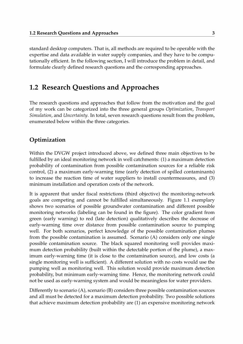
It is apparent that under fiscal restrictions (third objective) the monitoring-networkgoals are competing and cannot be fulfilled simultaneously. Figure 1.1 exemplaryshows two scenarios of possible groundwater contamination and different possiblemonitoring networks (labeling can be found in the figure). The color gradient fromgreen (early warning) to red (late detection) qualitatively describes the decrease ofearly-warning time over distance from possible contamination source to pumpingwell. For both scenarios, perfect knowledge of the possible contamination plumesfrom the possible contamination is assumed. Scenario (A) considers only one singlepossible contamination source. The black squared monitoring well provides maxi-mum detection probability (built within the detectable portion of the plume), a max-imum early-warning time (it is close to the contamination source), and low costs (asingle monitoring well is sufficient). A different solution with no costs would use thepumping well as monitoring well. This solution would provide maximum detectionprobability, but minimum early-warning time. Hence, the monitoring network couldnot be used as early-warning system and would be meaningless for water providers.

Differently to scenario (A), scenario (B) considers three possible contamination sourcesand all must be detected for a maximum detection probability. Two possible solutionsthat achieve maximum detection probability are (1) an expensive monitoring network

4 Introduction

including the white and blue monitoring wells, or (2) the less expensive monitoringnetwork with a single green monitoring well that monitors all three sources simultane-ously in one point. Drawback of the single monitoring well is the lower early-warningtime due to the late detection of all three sources. Less expensive trade-off networksthat do not seek for maximum detection probability can increase early-warning timefor selected possible contamination sources by shifting their focus to selected sourcesand ignoring the others. Thus, the selected sources can be detected as early as possible(e.g., white monitoring well, or both blue monitoring wells).

In conclusion, the three objectives are conflicting and it is impossible to find the perfectmonitoring network that completely satisfies all three objectives simultaneously, i.e., amaximum detection probability, a maximum early-warning time, but no costs. Rather,many trade-off solutions can be found with a different balance between the three ob-jectives. For finding these trade-off solutions, formal optimization can be applied tothe problem. Due to the conflicting objectives, the general optimization approach is toformulate the problem as a multi-objective optimization problem and to translate theobjectives in quantifiable objective functions. For large and complex problems, how-ever, the optimization might need long wall-clock times to find (eventually) satisfyingsolutions. Consequently, the first two research questions are:

1. How can I formulate the optimization problem for an effective optimization?

(A)

(B)

MonitoringWells

Gradient of Early-Warning Time

PumpingWell

Possible Contami-nation Source

1

Figure 1.1: Two different scenarios of possible groundwater contamination. Scenario(A): A single possible contamination source can be monitored by a single monitoringwell that should be close to the possible contamination source for early warning. Sce-nario (B): Multiple possible contamination sources need monitoring. Three monitoringnetworks (green countered square, white and blue contoured squares, white contouredsquare) satisfy the three objectives to different degrees that cannot be fulfilled simulta-neously.

1.2 Research Questions and Approaches 5

2. How can I speed up the optimization (improve efficiency), improve optimizationquality (increase effectiveness), and minimize quality variability of optimizationresults (increase reliability)?

Transport Simulation

Irrespective of the optimization results, the optimization is based on data from numer-ical transport simulations. Developing the corresponding transport models is difficultand time-consuming. First, transport relevant model parameters and boundary con-ditions are subject to uncertainty (see next category below). Second, the possible con-tamination sources form the source terms of transport simulation. Hence, water sup-pliers need to collect a lot of information from their well catchments as model inputdata. Here, the most challenging part is to identify all relevant possible contaminationsources and to prioritize them according to their risk for the production wells. Thisprioritization is important for the monitoring-well design that should especially mon-itor the most dangerous possible contamination sources. While the identification ofpossible sources is mostly laborious work, their risk quantification is often impossible.Too many data are unknown, e.g., the probability of failure, or the type and amount ofharmful substances that are stored at the location of question. Therefore, the next tworesearch questions are:

3. How can I support the data collection of the water suppliers and help to distin-guish between relevant and irrelevant possible contamination sources?

4. How can water suppliers prioritize the relevant possible contamination sourcesaccording to their risk without the data required for a quantitative risk assess-ment?

Uncertainty

In addition to the challenges introduced above, finding optimal positions of monitor-ing wells is also challenging because various parameters influence the reliability andoptimality of a suggested monitoring location and are often subject to uncertainty:

• There may be uncertainty in hydro(geo)logy, i.e., in global and local velocityfields, which can vary in angle and absolute value.

• There may be uncertainty in the exact position of possible contamination sources,or even worse, there may be possible contamination sources that are unknown inexistence, hence in location.

• There may be uncertainty in transport-relevant parameters that describe, e.g.,dispersion and decay.

6 Introduction

• There may be uncertainty in the spilled mass of contamination when a possiblecontamination source fails.

The resulting research questions are:

5. How can I consider in a computationally feasible way the uncertainty in hy-dro(geo)logy, transport-relevant parameters, and location of possible contami-nation sources to get optimization results that are robust against uncertainty?

6. How can I consider unknown possible contamination sources?

7. How can I verify optimization results under uncertainty?

Summarized, in this thesis, I investigate and present a framework that enables watersuppliers to optimize their monitoring networks according to the three objectives de-tection probability, early-warning time, and costs on standard desktop computers. Thekey approaches cover

• the multi-objective optimization problem formulation,

• the data collection and transport simulation,

• and uncertainty representation for a robust optimization.

1.3 State of the Art

The general field of groundwater monitoring is huge and research is going in diversedirections. Two main categories are the monitoring of groundwater levels and themonitoring of groundwater quality. In this thesis, the second category is relevant andcan further be divided into two classes:

1. Monitoring of existing groundwater contamination, and

2. monitoring of potential groundwater threats to safeguard groundwater quality.

For the first class of monitoring networks, the objectives can still be manifold. Typ-ical tasks for existing plumes are to find the shape of the contamination plume [e.g.,9, 108] for better taking countermeasures, to estimate the contaminant discharge [e.g.,99, 145, 161] for a better risk-assessment of the contaminant plume, or to identify con-taminant sources [e.g., 66, 119, 139] for permanent and effective counter measures. Thesecond class of monitoring networks focuses on protecting source water for water-supply companies against possible future contamination events. Differently to the firstclass of monitoring networks, here the networks are typically large-scale and long-termgroundwater monitoring networks (see review by Loaiciga et al. (1992) [106] and thecomprehensive review in the work of Kollat et al. (2011) [96]).

1.3 State of the Art 7

As already said in Section 1.1, for reducing the risk evolving from these possible fu-ture contamination events, the most common measure is to restrict the land use withinwell protection zones [e.g., 46, 164]. However, with growing urban density and con-tentious competition over highly valued land uses, it is becoming increasingly difficultto characterize and manage source water well protection zones, especially in rapidlyexpanding cities. Additionally, there is uncertainty in the actual outline of the wellcatchment. Thus, there is always an inventory of possible contamination sources in thecatchment that remains to be assessed and controlled. Accordingly, there is ample liter-ature on capture zone delineation and its uncertainty [e.g., 80, 120, 153, 167], on aquifervulnerability [e.g., 4, 44, 184], on (probabilistic) well vulnerability [e.g., 51, 52, 60] andon risk analysis [e.g., 28, 159]. While such works help to evaluate the possible contam-ination sources to which the production well is exposed, they are not yet helpful incontrolling them.

These contamination detection problems are also closely related to early work focusedon monitoring of landfills [e.g., 111, 112, 117, 118, 154]. Although early work such asMassmann and Freeze (1987a,1987b) [111, 112] performed a single-objective risk-cost-benefit analysis to optimize and evaluate the quality of monitoring networks, thereis a growing trend in the monitoring literature towards formulations that considermultiple objectives and multi-objective optimization. Commonly employed objectivesinclude maximizing the detection probability, minimizing costs, and minimizing thecontaminated area, or the volume of contaminated groundwater, respectively, [e.g.,118, 154, 179]. The last of these objectives is indirectly related to the objective of earlydetection of a contamination that would provide benefits in remediation costs and re-source protection. In my approach, however, an early detection gains benefits in thereaction time of water suppliers to install countermeasures for well-head protection ofthe production wells. The monitoring network is used as early-warning system. Mon-itoring networks as early warning systems are often associated with disaster manage-ment for natural hazards such as tsunami or earthquake warning systems, e.g., Allenand Kanamori (2003) [3]. Alternatively, there is research on detection sensor networksin the signal processing literature [e.g., 115], but without existing applications to wellcatchments. Therefore, the major differences between my approach and the namedstudies are:

1. They do not consider the protection of groundwater wells against a whole inven-tory of possible contamination sources. Instead, they focus on monitoring of asingle landfill.

2. My approach considers a significant number of candidate monitoring locationsand therefore poses a severely challenging multi-objective combinatorial prob-lem.

8 Introduction

1.4 Contributions and Structure of the Work

This thesis is structured into eight chapters that can be divided into three parts:

Introduction and Background After the introduction in the current Chapter 1, Chap-ter 2 introduces the fundamentals and background of the following chapters. Thesechapters do not contain any novelties or contributions.

Contributions Chapters 3, 4, 5, and 6 form the main part of this thesis and containmy own contributions:

• In Chapter 3, I formulate the optimization problem and develop the objectivefunctions. These objective functions relate to the efficiency, effectiveness, androbustness of the monitoring network. Here, I also introduce two benchmark testcases that I developed and that are used in the following chapters.

• In Chapter 4, I tackle performance problems of multi-objective optimization al-gorithms for large and complex, discrete multi-objective optimization problems.The focus is on search-space representation and search-space reduction to achieveefficiency, effectiveness, and reliability of the optimization process.

• In Chapter 5, I develop feasible methods regarding transport simulation, riskassessment, and robust multi-objective optimization for an improved search foroptimal early-warning monitoring networks in practice. These methods illustratethe achievable transfer to practice.

• Finally, in Chapter 6, I introduce analytical solutions that help understand opti-mization results given parameter uncertainty.

Application and Summary In Chapter 7, I apply the optimization framework on areal case from a local water-supply company. I also discuss strategies for a successfultransfer from academia to practice, lessons we have learned during the project I intro-duced in Chapter 1. The last chapter (Chapter 8) contains a summary and the mainconclusions of this thesis. Finally, I briefly introduce possible future investigationsevolving from the discussed methods in the previous chapters.

Relation to Published Works

This dissertation is based on several publications including Nowak et al. (2015) [126],Bode et al. (2016a) [19], Emmert et al. (2016) [48], Bode et al. (2017) [14], Bode

1.4 Contributions and Structure of the Work 9

et al. (2018b) [15], Bode et al. (2018c) [21] (submitted), and Bode et al. (2018a) [13](in preparation). Chapters 1, 2, and 8 may contain similar and/or identical formula-tions from these works, but do not contain any scientific novelties and contributions.Therefore, I omit a clear identification in these chapters. The remaining contributingchapters include general but unique references of the sources in the very beginning ofeach chapter.

I presented most of my results on a number of international conferences, including

• AGU 2013-2016: Bode et al. (2013, 2014c, 2015, 2016b) [10, 16, 22, 20]

• EGU 2015: Bode et al. (2015) [17]

• NGWA 2014: Bode et al. (2014a) [11]

• CMWR 2014: Bode et al. (2014b) [12]

• NUPUS 2013: Bode and Nowak (2013) [18]

Finally, this thesis played an important rule on the methodical level within in the jointresearch project Risk-Based Groundwater Monitoring for Well Head Protection Areas to-gether with the DVGW and the related final report [67]. Following the project, theresults should also be used to revise the technical guideline W108 [45].

Chapter 2

Fundamentals

In this chapter, I give a brief introduction to all fundamentals relevant for understand-ing this thesis. In Section 2.1 I introduce the governing equations of groundwater flowand transport. The following two sections introduce possible approaches to solve thegoverning equations, ie.e, analytical solutions in Sections 2.2 and numerical methodsand established software in Section 2.3. Sections 2.4 and 2.5 are related to locationsand levels of uncertainty within the scientific workflow of modeling and to uncertaintyquantification. Section 2.6 gives a brief introduction to optimization and an overviewof different optimization techniques with the emphasis on multi-objective optimiza-tion. Finally, Section 2.7 introduces metrics that help evaluate the performance of opti-mization algorithms.

2.1 Governing Equations of Flow and Transport in

Porous Media

Steady-State Flow in Confined Aquifers

Steady-state groundwater flow in confined aquifers can be described by

−∇ · (K∇h) = qs in Ω, (2.1)

with hydraulic conductivity K [L/T], hydraulic head h [L], and source and sink term qs[L2/T

]in the domain Ω [8]. Equation 2.1 is subjected to the general boundary condi-

tions:

− (K∇h) · n = q on Γ1 and (2.2)

h = h on Γ \ Γ1, (2.3)

using the prescribed fluxes q and heads h on the Neumann boundary Γ1 and on theDirichlet boundary Γ \ Γ1. The normal vector n points outwards on the domain. Inconfined aquifers, vertical flow is often negligible in relation to the horizontal flow.Then, the conductivity K can be substituted by the depth-integrated transmissivityT = K · B, with B [L] as the aquifer thickness. Equation 2.1 adopts to

−∇ · (T∇h) = qs , (2.4)

2.2 Relevant Analytical Solutions 11

and is also known as the two-dimensional, depth-averaged groundwater-flow equa-tion.

Transport of Conservative Tracer

The advective-dispersive transport of conservative tracers is commonly described bythe advection-dispersion equation (ADE):

∂c

∂t+∇ · (vc − D∇c) = 0 in Ω, (2.5)

with concentration c [M/L3], time t [T], velocity v = qne

[L/T] and Darcy velocity q

[L/T], effective porosity ne [−] and hydromechanic (or macroscopic) dispersion tensorD[

L2/T]

[143]:

D = (αt‖v‖+ Dm) I + (αℓ − αt)vvT

‖v‖ . (2.6)

Here, αℓ and αt (both [L]) are the longitudinal and transverse dispersivities, Dm[

L2/T]

is the molecular diffusion coefficient, and I is the identity matrix. The boundary con-ditions for Equation 2.5 are given by:

−n · vc + n · (D∇c) = J on Γ2 and (2.7)

c = c on Γ \ Γ2, (2.8)

with J as a prescribed normal flux density and c as prescribed concentrations. Understeady-state conditions, the first term in Equation 2.5 becomes 0 and the advective-dispersive transport is described by:

∇ · (vc − D∇c) = 0 . (2.9)

2.2 Relevant Analytical Solutions

Spatial Concentration Distribution

For parallel flow with a uniform dispersion coefficient D and uniform velocity v, Equa-tion 2.5 can be written as

∂c

∂t+ v · ∇c −∇ · (D∇c) = 0 . (2.10)

12 Fundamentals

For a continuous point-like injection of a conservative tracer, a two-dimensional ana-lytical steady-state solution for Equation 2.10 is given by

c (x, y) =min

B

1√4πvxDT

· exp(− y2v

4DTx

). (2.11)

Here, the longitudinal dispersion DL[

L2/T]

was neglected, because the point sourceis a continuous injection. Then, the longitudinal dispersion plays only a minor rolefor the concentration distribution in space [e.g., 73]. For the sake of completeness, aderivation of Equation 2.11 can be found in Appendix A.1. Equation 2.11 provides anexpression for the aqueous contaminant concentration c [M/L3] at any point (x, y) atsteady state due to a continuous injection with mass discharge min [M/T], aquifer thick-ness B, groundwater-flow velocity v, and transverse dispersion coefficient DT

[L2/T

].

Breakthrough Curve

For a simple groundwater model with uniform and parallel flow and uniform dis-persion coefficient, the shape of a unit-mass breakthrough curve of a point-like andinstantaneously injected aqueous contaminant mass can be calculated analytically andis given by the inverse Gaussian distribution (IG) [e.g., 57] (cf. Figure 2.1). For thesegroundwater models the assumption of Fickian transport is valid [e.g., 7], i.e., disper-sion can be modeled as Brownian motion. The probability density function (pdf) of theinverse Gaussian distribution is given by

f (t; µ, λ) =

(λ

2πt3

) 12

· exp

(−λ (t − µ)2

2µ2t

), (2.12)

for time t > 0. It is fully described by the mean µ > 0 and the shape parameterλ > 0. The shape parameter λ is a function of the mean and the variance σ2 and can be

calculated as λ = µ3

σ2 .

Accordingly, the analytical shape of the breakthrough curve of a continuous pointsource is given by the cumulative distribution function (cdf) of Equation 2.12 (cf. Fig-ure 2.1):

F (t; µ, λ) =12

1 + erf

√λt

(tµ − 1

)

√2

+ exp

(2λ

µ

)

12

1 + erf

−√

λt

(tµ + 1

)

√2

(2.13)

2.3 Numerical Solutions of Flow and Transport 13

In applications, both functions have to be scaled to calculate the time-dependent con-centration distribution c (t). The corresponding scaling factor depends on the prop-erties of the contaminant and the release conditions. A detailed explanation on thederivation of this scaling factor can be found in Section 5.1.

2.3 Numerical Solutions of Flow and Transport

Analytical solutions are only valid for strongly simplified problems. Realistic prob-lems, however, are highly complex, hence groundwater flow and transport (Equa-tions 2.1 and 2.5) cannot be solved analytically anymore. Instead, numerical simulationtechniques are used.

Numerical methods can roughly be distinguished between Eulerian and Lagrangian.Eulerian methods apply mass balance on fixed control-volumes to approximate the un-known quantity (e.g., flow velocity of water). Lagrangian methods are based on mov-ing parcels, approximating the unknown quantity by tracking discrete parcels overspace and time. Two well-known representatives of the Eulerian method are the finitedifference method (FDM) [e.g., 149] and the finite element method (FEM) [e.g., 180].Representatives of Lagrangian methods are the particle tracking method (PT) [e.g., 130]and the particle-tracking-random-walk method (PTRW) [e.g., 56, 84, 102, 140, 172]. Ingroundwater modeling, Eulerian methods are usually used to approximate ground-water flow and complex multiphase multicomponent transport processes. Lagrangian

0 2.5 50

0.5

1

pdf

cdf

µ = 1λ = 2

1

Figure 2.1: Inverse Gaussian distribution: Probability density function (pdf) as ana-lytical solution for the shape of the breakthrough curve of an instantaneous point-likecontaminant injection, and the cumulative distribution function (cdf) as solution forthe continuous injection.

14 Fundamentals

methods are used for simple transport processes.

In practice, two established software for developing and simulating numerical ground-water models are ModFlow [74] and FeFlow [39, 160]. Both software are widely spreadamong groundwater-related engineering companies and water suppliers. While Mod-Flow is based on a finite difference method to solve the groundwater flow equation,FeFlow calculates the velocity field using a finite element method. Most of the velocityfields I use in this thesis are created by an in-house FEM code as described in Nowaket al. (2008) [127].

Solving the flow equation with Eulerian methods (like FEM or FDM) is neither chal-lenging nor computationally expensive. For transport simulation, however, thesemethods are very expensive and prone to oscillation and numerical dispersion. Incontrast, the Lagrangian-based PTRW method is simple to implement, fast, robust,and free of numerical dispersion and oscillation [e.g., 140]. In the following section, Idescribe this method in detail.

Particle-Tracking-Random-Walk

Unlike particle tracking, PTRW is not a deterministic method as it includes a modelto simulate the random diffusion/dispersion behavior of virtual solute particles ingroundwater flow. This model assumes Fickian transport laws and, strictly spoken,is only valid on fully resolved velocity fields (i.e., at which the parameterization ofdispersion through enhanced diffusion is valid).

The approximation of the steady-state ADE (Equation 2.9) is given by an ensemble ofparticles driven by advection and dispersion:

Xp (t + ∆t) = Xp (t) + ∆Xp (t + ∆t) , (2.14)

with the particle position Xp [L], the particle displacement ∆Xp [L], time t [T] and timediscretization ∆t [T]. The particle shift ∆Xp is obtained by

∆Xp (t + ∆t) = u∗∆t + B(Xp, t

)√∆t · ξ (t) , (2.15)

with the deterministic drift u∗ =(u(Xp, t

)+∇ · D

(Xp, t

))that is determined by

the velocity u and the gradient of the dispersion tensor D, and the stochastic termB(Xp, t

)√∆t · ξ (t), with the displacement matrix B that scales a vector of standard

normally distributed random variables ξ. The displacement matrix B has to fulfill thecondition B · BT = 2D. Following Salamon et al. (2006) [140], for three-dimensionalproblems B can be calculated as

B =

ux|u|wℓ − uxuz

|u|√

u2x+u2

ywt − uy√

u2x+u2

ywt

uy

|u|wℓ − uyuz

|u|√

u2x+u2

ywt

ux√u2

x+u2ywt

uz|u|wℓ

√u2

x+u2y

|u| wt 0

, (2.16)

2.4 Sources of Uncertainty Considered in this Work 15

with wℓ =√

2 (αℓ |u|+ Dm) and wt =√

2 (αt |u|+ Dm).

Finally, at each location, the temporal evolution of particle densities can be used toestimate breakthrough curves. If the number of particles is large enough, it can bedone by direct density estimation. Otherwise, if the number of particles is too smallfor a direct estimation, one can use a parametric density estimation [e.g., 49], e.g., byusing Equations 2.12 and 2.13 introduced in Section 2.2.

Reverse Particle-Tracking-Random-Walk

Reverse particle-tracking-random-walk (RPTRW) is a concept that enables, for in-stance, to localize the catchment of drinking-water wells with a single simulation. Thebasic idea behind this concept is to reverse the entire velocity field and inject a unitmass at the pumping wells [e.g., 60, 100, 121]. Then, transport is solved reverselyby applying the PTRW method. The boundary conditions have to be adjusted prop-erly, based on the boundary conditions of the forward transport simulation. For bothmethods (PTRW and RPTRW) I used an already existing code also used in Koch andNowak (2014, 2015, 2016) [90, 91, 92] and Bode et al. (2016a) [19].

2.4 Sources of Uncertainty Considered in this Work

Decision-supporting models are usually affected by many sources of uncertainty.Walker et al. (2003) [169] generalized uncertainties according to their location in themodeling process and defined the following five types of uncertainty:

1. Context uncertainty refers to the problem and the purpose of the model. If problemand purpose are not defined clearly, the model outcome can be highly uncertain.For instance, a model for predicting water levels of a lake can neither be used toforecast water levels of a river nor to predict the damage caused by a flood.

2. Model uncertainty describes the uncertainty related (1) to the choice of the con-ceptual model, i.e., the mathematical equations, and (2) to their computationalimplementation.

3. Parameter uncertainty is associated with the data used for model calibration, aswell as the calibration method itself. While some parameters are known withcertainty (e.g., universal constants like π), unknown parameters are determinedby calibration, hence are affected by measurement errors of the calibration dataand the setup used for calibration (method, level of accuracy, grid resolution,etc.).

16 Fundamentals

4. Input uncertainty refers to all data that describe the reference system. Input is af-fected by uncertainty (1) due to external driving forces that might underlie naturalvariabilities (e.g., the evaporation of water is related to solar radiation), and (2)due to a lack of knowledge about system relevant data (e.g., pumping rate of agroundwater extraction well).

5. Model outcome uncertainty describes the prediction error that is caused by the typesof uncertainty introduced above.

In this work, I will only consider parameter and input uncertainty (in the following, Iwill address both as parameter uncertainty) for three reasons:

1. This work is strongly influenced by requirements and limitations of practical ap-plications because results should be used by water suppliers. The models typi-cally used by water suppliers have already been developed with substantial fi-nancial investments, and concepts and their mathematical implementation aremostly limited to the software that was decided to be used many years ago. In-vestigating model uncertainty for concepts that are not predefined in the modelsof the water suppliers (e.g., dispersion models) would be too time-consuming forthe practical use.

2. In this work, model outcome uncertainty is dominated by parameter uncertainty.For instance, uncertainty in ambient flow direction causes large uncertainty in thelocation of a contaminant plume. Then, for water suppliers, it is more importantto identify the possible contaminated area than possible tailing in contaminantbreakthrough curves due to different dispersion models.

Therefore, context and model uncertainty is not within the scope of this work. By onlyconsidering parameter uncertainty, I assume that all used mathematical equations aresufficiently close to the real processes that govern the system so that models predictthe real physical states of the systems reasonably well. The parameters I considered asuncertain are

• the permeability field (heterogeneity concepts: layering, zonations, and geostatis-tics),

• boundary conditions of flow and transport,

• sink and source terms, and

• transport relevant parameters.

A detailed description of how I considered uncertainty can be found in the relevantsections (Sections 3.5 and 6.3).

When discussing uncertainty, I also follow the terminology of Walker et al. (2003) [169]regarding the uncertainty level. They distinguish between three types of uncertainty

2.5 Uncertainty Quantification with Monte-Carlo Methods 17

levels: statistical uncertainty, scenario uncertainty, and recognized ignorance. Statisticaluncertainties can be described by probability distributions and hence are quantifiable.Scenario uncertainty does not have a known probability distribution, but its effectscan be investigated by making assumptions about the uncertain parameters to createpossible scenarios: scenario uncertainty can describe possibilities but without assignedprobabilities. Recognized ignorance contains uncertainty that is known to exist butignored because neither probability distributions are known nor the behavior suchthat useful assumptions can be made to express it as scenario uncertainty. These threeuncertainty levels are bracketed by the two extrema of determinism, where everythingis known, and total ignorance, where it is unknown what is unknown. With the termuncertainty, I refer to scenario uncertainty unless specified otherwise.

2.5 Uncertainty Quantification with Monte-Carlo

Methods

In the field of uncertainty quantification, Monte-Carlo (MC) methods are often usedto analyze the statistical distribution of a deterministic model outcome. While theidea of MC methods is dating back to the Babylonian era [72], Metropolis andUlam (1949) [116] labeled it and established a systematic use. The basic idea of MCmethods is to run a model multiple times with random but equally likely model inputparameters and so approximate the distribution of the model outcome. Each set of in-put parameters is called MC experiment and the model outcomes are called realizations.Then, the distribution of realizations can be analyzed statistically. Many different MCmethods exist, which mostly differ in the sampling rule of the model input parameters[e.g., 137]. The three main steps of MC methods are:

1. Input parameter set: Multiple sets of input parameters have to be generated,based on the distribution of the input parameters, and based on a specified sam-pling rule.

2. Model run: Each parameter set triggers a (deterministic) model run.

3. Statistical analysis: The set of realizations is evaluated via, e.g., histograms orprobability density estimators.

MC methods are computationally expensive and they require a large number of real-izations for a good approximation of the model outcome distribution. However, theyare intuitive, easy to implement, and independent of the model.

18 Fundamentals

2.6 Optimization

The following introduction to optimization problems is based on the work of Zitzleret al. (2004) [181] and on the book of Talbi (2009) [157]. In general, an optimizationproblem is the search for the best solution according to a certain criterion from all fea-sible solutions within the search space Ω. Mathematically, the criterion can be expressedas an objective function f that maps possible solutions from the search space Ω to theobjective space Y:

f : Ω → Y . (2.17)

The outcome of f is an objective vector y = (y1, y2, . . . , ym) ∈ Y . The challenge is to finda solution x = (x1, x2, . . . , xn) ∈ Ω such that f (x) is either minimal or maximal. Inthe following, all problems are defined as minimization problems. That is, the globaloptimum x∗ ∈ Ω satisfies the following constraint:

∀x ∈ Ω , f (x∗) ≤ f (x) . (2.18)

In the case that Y is a subset of the real numbers (Y ⊆ R), the problem is a standardsingle-objective optimization problem with a scalar-valued objective function f . Al-though there might be more than one optimal solution, Equation 2.18 can be fulfilledbecause all optimal solution vectors x are mapped to the same scalar objective value y.

If the objective function f consists of multiple sub-functions f and Y ⊆ Rm with m > 1,

the problem is called a multi-objective optimization problem. Then, optimal solutions x

might be mapped to different objective vectors y such that a global optimum is notnecessarily existent. In this case, the comparison of two solutions x1 and x2 is morecomplex and follows the principle of Pareto dominance [128]: the assigned objectivevector y1 dominates y2 if no component of y1 is greater (less good) than a componentof y2 and at least one component of y1 is smaller (better). Mathematically, this domi-nance is expressed as y1 ≺ y2. In this case, solution x1 is said to dominate solution x2.Solutions that are not dominated by any other solution x ∈ Ω are called non-dominated

solutions or Pareto-optimal solutions. The Pareto set contains all Pareto-optimal solutionsand is a subset of the search space Ω. The Pareto front is the image of the Pareto-optimalsolutions in the objective space and is a subset of the objective space Y.

There are two main classes of optimization models to formulate and solve the opti-mization problems: linear programming (LP) and nonlinear programming (NLP). Further,these models can be divided into continuous problems and discrete problems, as well aslow-dimensional problems and high-dimensional problems.

Linear programming is a model where the objective function, as well as the constraintsof the optimization problem, are both linear. LP is relatively easy to solve and thereare efficient and exact optimization algorithms (e.g., the simplex algorithm [29]). Thebeauty of LP is that the search space (determined by the constraints) and the objective

2.6 Optimization 19

Objective Function 1

0 0.5 1

ObjectiveFunction2

0

0.5

1

1Figure 2.2: Two-dimensional Pareto-front for two objective functions. The Pareto frontis a set of non-dominated solutions (red spheres) and dominates all solutions that arenot Pareto optimal (dominated solutions in black/gray). The color of the dominatedsolutions changes from black to transparent gray regarding their distance towards thePareto front.

function are convex. Hence, either the global optimum can be found on the contactpoint between objective function and the search space Ω, or the objective function isparallel to the edge of the search space Ω and each found optimum is a global opti-mum.

Problems with a nonlinear objective function and/or nonlinear constraints have to besolved with nonlinear programming. The search space Ω of NLP problems is a subsetof R

n where n is the number of modifiable influencing parameters of the problem.For low-dimensional problems, n is small, while for high dimensional problems n isa large number. An example of a low-dimensional problem is the optimization of aflight trajectory of a cannonball: for covering the longest possible distance, one canonly modifying the shooting angle (n = 1). An example of high-dimensional problemsis the optimization of a monitoring network with a large number of possible locationsfor monitoring wells.

Continuous optimization problems differ from discrete problems in the composition ofthe search space Ω. Continuous problems are related to continuous search spaces, i.e.,the number of solutions is infinite. Discrete problems are often combinatorial problemsand are based on a finite set of solutions, although the number of solutions might runtowards infinity for large problems.

The choice of the best optimization algorithm to solve the problem depends on the

20 Fundamentals

optimization problem itself (following the No Free Lunch theorem by Wolpert (1995,1997) [177, 178]). For instance, efficient and exact algorithms exist for a continuous,quadratic, convex problem [e.g., in 125]. However, for NLP, it is often unknownwhether a problem is convex or not. Thus, many local optima might exist and thesearch for a global optimum is computational very expensive. Then, so-called meta-

heuristics come into play that do not aim to find the global optimum, but a sufficientlygood approximation. In the following section, I will give a brief overview of commonoptimization methods with a focus on meta-heuristics.

2.6.1 Optimization Techniques and Optimization Algorithms

The easiest optimization problems are posed by differentiable functions with a closed-form expression of the derivative. To solve such problems, the first derivative locatesthe extrema and the second derivative defines whether these extrema are local maximaor minima To find the global optimum, local optima just have to be compared.

Functions that are differentiable but do not have a closed-form derivative cannot beoptimized analytically. When it is known a priori that the problem has a global opti-mum but no local optima (e.g., in convex problems), gradient-based optimization methods

are a good choice to apply. For gradient-based methods, it is not important to knowthe function to be optimized in an explicit way. However, the function value and thegradient at each point has to be calculable. Then, these methods start from an arbitrarypoint and always go in the direction of the negative slope.

These methods can also be applied to functions with local optima (e.g., non-convexproblems) but either the algorithms need modifications for being able to leave a localoptimum, or the search for the global optimum is done multiple times with randomstarting points. As a result, the solution time for non-convex problems can be verytime consuming, especially for large problems. One of the most famous algorithms isthe Gradient Descent [e.g., in 107, here labeled as Gradient Ascent], which only uses theinformation of the first derivative. Modifying the Gradient Descent method using alsothe second derivative results in the well-known Newton Method [e.g., 38].

Large-size non-convex problems can be tackled by meta-heuristics. Although there isno guarantee that they will find the global optimum, it has already been shown thatthey are very efficient and effective. That is, they approximate the global optimumin an acceptable time. Many classifications of meta-heuristics exist, e.g., deterministicand stochastic search, or population-based and single-solution based search.

The Simulated Annealing algorithm [24, 85] can be classified as a stochastic and single-solution based search. Stochastic, because the algorithm uses partially randomizeddecisions in its rules towards the optimal solution, and single-solution based, because

2.6 Optimization 21

at the same time the algorithm considers only one possible solution. Simulating An-nealing is based on the so-called Hill-Climbing Algorithm, which tests solutions aroundthe current solution and replaces the current solution when a better one is found inthe neighborhood. Simulated Annealing differs from the Hill-Climbing algorithm atthe replacement step of the current solution: Simulated Annealing always replaces thecurrent solution if the new solution is better. If the new solution is worse, the cur-rent solution will be replaced with a certain probability that depends on the differencebetween the current and the new solution, and a parameter t. Initially, t has a highvalue, but over iterations, t decreases (t can be seen as temperature what also explainsthe name of this algorithm: the temperature cools down (anneals) over time). A highvalue in t means that the probability of accepting worse solutions is high and the al-gorithm randomly explores the search space. Contrary, a decreasing t means that theacceptance rate decreases and the algorithm exploits the current region of the searchspace.

Differently to Simulated Annealing, the algorithm Tabu Search by Glover (1986) [62],also contains memory of the search process. That is, Tabu Search includes a list ofsolution candidates the algorithm already explored and refuses to get back to thesesolutions. Consequently, Tabu Search only works for discrete problems, otherwise,the memorized Tabu-list would be infinite, and therefore useless. Candidate solutionswithin this list are released after a certain optimization time or a certain number ofiteration steps. This list enables the algorithm to leave local optima by forcing it to ex-plore neighboring regions that might be worse but in the direction of a better solution.Extensions of this algorithm include different memory lists, e.g., to avoid the loss of al-ready found good solutions, and to provide a diverse search that supports a sufficientdegree of exploration.

Population-based meta-heuristics explore the search space simultaneously with manysolution candidates. These solution candidates communicate among each other and useswarm intelligence to find the optimal solution. Examples of popular algorithms arethe Ant Colony Optimization (ACO) [43], the Particle Swarm Optimization (PSO) [83], andEvolutionary algorithms (EAs).

ACO is based on the efficiency of an ant colony to find the shortest way to a foodsource. An obstacle that is between the ants and the source must be bypassed, eitherclockwise, or counter-clockwise. In the beginning, the probability for both sides is thesame. If one of the two ways is shorter, over time, the shorter way enables the ants tobe faster in collecting the food and the shorter trail is used more often. After a while,the shortcut is full of pheromones, a substance ants are using for communicating andthe other ants will also use the shortcut. Thus, to apply ACO, optimization problemshave to be formulated as pathways.

PSO is based on fish schools or bird flocks that search for good food places. Each par-ticle (fish or bird) represents a solution candidate of the optimization problem and all

22 Fundamentals

particles explore the search space. The individual change in their locations within thesearch space follows rules that consider (1) the position of the best solution each indi-vidual particle has discovered yet, (2) the position of the best solution the neighboringparticles have discovered yet, and (3) the position of the best solution all particles havediscovered yet. Together, the particle swarm is moving towards the optimal solution.

EAs are optimization methods that are based on natural evolution. Research on EAswithin the last few decades has shown that they can handle large and complex searchspaces and are easily and successfully adaptable to multi-objective problems. Thus,EAs designed for solving multi-objective optimization problems are called multi-objective evolutionary algorithms (MOEAs). In this thesis, I use an MOEA to solvethe optimization problem. Many studies have shown that MOEAs can handle chal-lenging optimization problems [see reviews of 109, 124]. In the following section, theprinciple of MOEAs is introduced more into detail. This introduction is based on thetutorial of Zitzler et al. (2004) [181].

2.6.2 Multi-Objective Evolutionary Algorithm - MOEA

As already mentioned above, MOEAs are evolutionary algorithms designed for solv-ing multi-objective optimization problems. They are population-based meta-heuristicsand explore the search space with many candidate solutions. The main principles ofMOEAs are selection and variation. Selection describes the competition for reproductionand resources, whereas variation describes the creation of new individuals by recombi-

nation and mutation. In MOEAs, an individual is a solution candidate of the optimiza-tion problem and a set of individuals are called population. The selection process isseparated into two different selections: the mating selection and the environmental se-

lection. While mating selection can roughly be described as a selection process due toassertiveness, the environmental selection is often described as survival of the fittest.

Mating selection is separated into two phases. First, the fitness of all individuals of thepopulation is determined by the objective functions (i.e., their quality). Second, themating pool is created by a sampling rule that selects the individuals regarding their fit-ness. An often used sampling rule is the so-called tournament selection, where a certainnumber of individuals is randomly drawn from the population and the individualsare compared by their fitness. The winner of the tournament becomes a member of themating pool. By doing many tournaments, one obtains a mating pool with many fitsolutions.

The mating pool (also called parent population) is treated by variation operators thatusually are members of the two overall classes recombination and mutation. Whilerecombination creates a predefined number of new individuals (called children andchildren population) by combining parts of a certain number of old individuals of the

2.6 Optimization 23

parent population (called parents), mutation modifies individuals by changing smallparts of them.

The environmental selection determines the composition of the new population byselecting individuals from the old, parent and children population. That is, MOEAshave a generational memory that stores the currently best approximation of the Paretoset and contains information that evolves over generations.

The procedure of MOEAs is illustrated in Figure 2.3: First, an initial population is cre-ated, either randomly or predefined with expert knowledge. Second, the basic stepsexplained above are iterated in a loop (mating selection, variation, environmental se-lection). Each loop iteration is called a generation. The goal of an MOEA is to find thebest approximation of the Pareto set (i.e., to minimize the distance of the approxima-tion set to the Pareto set) and to cover the complete Pareto set (i.e., to maximize thediversity of the approximation set). That is, the goal of an MOEA is multi-objectiveitself: proximity and diversity. Proximity is mainly related to the mating selection. Agood choice of parent population pushes the search of optimal solutions in the rightdirection. Diversity is related to selection in general. For instance, a selection opera-tor that only draws the same solution from a population leads to no diversity. Bothgoals, diversity and proximity, are also influenced by the so-called elitism, a term thatdescribes how to prevent the loss of solutions from the currently best approximationset. In the following, I introduce strategies to improve the optimization quality (i.e.,diversity and proximity) and speed.

Fitness Assignment The fitness assignment of MOEAs can be classified into three ba-sic categories: the aggregation-based, the criterion-based and the Pareto-based strate-gies. While the aggregation-based strategies aggregate the objective functions to a sin-gle fitness function (e.g., via a weighted mean with randomly drawn weights suchthat each individual has a different direction [71, 79]), criterion-based methods just

Initial Population

Selection

Mating

Environmental

FitnessEvaluation

Variation

Mutation

Recombination

ParentPopulation

ChildrenPopulation

Memory

New Population

FitnessEvaluation

Figure 2.3: Sketch of an MOEA. An optimization run starts with the initial population,followed by the illustrated iterative loop. The iteration is called generation.

24 Fundamentals

use one single objective-function value to assign a fitness value to each individual[e.g., 101, 142]. Goldberg (1989) [63] introduced first Pareto-based strategies, wherethe fitness of each individual is related to Pareto dominance. Three main approachesevolved from this basis: the dominance rank [58] that is related to the number of indi-viduals which dominate the assessed individual, the dominance count that is related tothe number of individuals that are dominated by the assessed individual, and the dom-

inance depth where the current population is subdivided into several fronts (the best isthe current approximation of the Pareto front) and the rank is the actual front number[e.g., 33, 152].

Elitism Elitism is an approach that prevents the loss of good solutions due to ran-dom effects during the optimization. An often used concept to avoid this loss is usingan archive. It serves as an external storage and contains all non-dominated solutionsand, in some cases, also promising but dominated solutions. Especially for continu-ous problems, storage problems might occur. Thus, dominance criteria (cf. paragraphabove) and density criteria (cf. paragraph below) are applied to reduce the number ofsolutions kept in the archive.

Diversity Preservation In multi-objective optimization problems, maximizing diver-sity is important, as the optimal result is not a single solution but a multi-dimensionalPareto front. The basis for most approaches to increase diversity is to acknowledgedensity information of the population during the selection process. That is, the proba-bility for an individual to be selected decreases when this individual has many neigh-boring solutions. The density is mostly evaluated in the objective space. Methods fordensity estimation include kernel methods (e.g., used in NSGA [152]) and nearest neigh-

bor methods (e.g., clustering in SPEA2 [182]). Basic methods for density estimation canbe found in Silverman (1986) [147]. They have in common that each solution mustbe compared with all other solutions. Two different approaches are the crowding dis-

tance (used in the NSGA-II [33, 36]) and the ǫ-dominance archive [introduced in 103](a variation is called ǫ-box dominance archive [e.g., 35, 94]). The crowding distance esti-mates the density of solutions surrounding a particular solution only on the same front(dominance depth). The ǫ-box dominance archive discretizes the objective space intohyperboxes (ǫ-boxes with the side-length ǫ). In each ǫ-box, only the non-dominatedsolution remains (the solution closest to the lower-left corner in a minimization prob-lem). Afterwards, dominance is related to ǫ-boxes and their lower-left corner.

Crossover and Mutation Operators As already mentioned above, the variation stepin MOEAs is based on crossover- and mutation-operators. Often used operators arethe Simulated Binary Crossover [32], Unimodal Normal Distribution Crossover [86], Sim-

plex Crossover [162], Polynomial Mutation [32] and Uniform Mutation. These operators

2.7 Metrics in Multi-Objective Optimization 25

explore the search space of the optimization problem differently. Thus, an adaptiveprobability-based use of them is recommended [e.g., 168, 69]. The probability of be-ing applied to the individuals is related to the number of produced solutions by eachoperator within the archive. That is, good performing operators are more likely to beapplied again.

Steady-State ǫ-MOEA Deb et al. (2003) [35] introduced a steady-state ǫ-MOEA thatfollows the idea of an ǫ-box dominance archive and differs from classical generationalMOEAs in the selection process for the mating. Instead of having just one populationthat evolves over the generations, a steady-state MOEA consist of two populations,the EA population, and the archive population. The mating happens between twosolutions from each population and their sizes remain constant. The archive size ispredefined by the number of ǫ-boxes. Details about the selection process and furtherimprovements can be found in Deb et al. (2003) [35], Kollat and Reed (2007) [94], andHadka and Reed (2013) [69].

2.7 Metrics in Multi-Objective Optimization

Performance metrics evaluate solution strategies of optimization problems. For single-objective optimization problems, the value of the objective function can be used di-rectly as a measure of quality: the smaller the objective value (in a minimization prob-lem), the better the solution. However, unlike single-objective optimization, the qual-ity of an approximation set from a multi-objective optimization cannot be evaluatedeasily. Although the concept of Pareto optimality defines whether a solution is non-dominated and belongs to the approximation set or not, it becomes more complexto compare the quality of two different approximation sets. For instance, approxi-mation set A could have a good proximity but is not diverse, while set B might beworse in proximity but good in diversity. Thus, the principle of Pareto optimalitycannot be used as metric to test whether approximation set A is preferred over set B.An overview of existing methods to measure the performance of multi-objective op-timization strategies can be found in Deb (2001) [31], Knowles and Corne (2002) [89],and Zitzler et al. (2003) [183]. Zitzler et al. (2003) [183] showed that optimization prob-lems need at least as many performance metrics as the number of objective functionsthe problem has, in order to compare two approximation sets unambiguously. How-ever, the main objectives of MOEAs are proximity and diversity of the approximationset [e.g., 23, 37]. Therefore, I introduce three performance metrics that focus especiallyon diversity and proximity: generational distance, hypervolume, and additive ǫ-indicator.Since the real Pareto front (PF) is usually not known, the approximation sets (AS)are compared with a reference set (RS), which is the best set of solutions known at

26 Fundamentals

this time. The following explanations and notations are based on the paper of Reedet al. (2013) [134].

(1) (2)

(3) (4)

Figure 2.4: Metrics to measure the quality of an approximation set. Multi-objectiveproblem with two objective functions (vertical and horizontal axes). Dashed line: Ref-erence set. Black dots: Approximation set. (1): Reference set and a good approxima-tion set. (2): Generational distance of an approximation set with a gap. The missingsolutions are marked in gray. The Euclidean distance from the approximation-set so-lutions to the reference set is illustrated as black lines. The gap has no influence onthis indicator. Its value only increases slightly due to the quality of the worse solution.Thus, it is an indicator only for proximity. (3): The additive ǫ-indicator is the distanceof the worst solution to the nearest solution of the reference set (illustrated as the blackline). A small value means that the approximation set is good in all of its solutions andhence it is consistent. (4): The hypervolume (shaded area) measures the volume that iscovered by the approximation set. A bad diversity/proximity decrease the hypervol-ume and hence it is a measure of both proximity and diversity. This figure is based onthe illustration of Hadka and Reed (2012) [68].

2.7 Metrics in Multi-Objective Optimization 27

Generational Distance The generational distance [e.g., 165, 166] (sub-figure (2) inFigure 2.4) measures the average Euclidean distance of the approximation-set solu-tions to the nearest solutions of the reference set. This proximity is represented by theindicator IG, calculated as follows:

IG (AS, RS) =

√∑x∈AS d2

x

NASS

(2.19)

with

dx = miny∈RS

√√√√NOF

∑i=1

( fi (x)− fi (y))2 .

Here, NASS is the number of solutions within the approximation set, NOF is the number

of objective functions, dx is the minimum Euclidean distance between the solutionsof the approximation set (x) and the reference set (y), and fi, i ∈ NOF is the set ofobjective functions.

Additive ǫ-Indicator The additive ǫ-indicator [183] (sub-figure (3) in Figure 2.4) isneither a good measure for proximity nor for diversity, but for consistency [68]. It mea-sures the smallest distance an approximation set has to move towards the reference setsuch that all solutions of the reference set would be dominated by the approximationset. This distance is given by the worst approximation-set solution, i.e., the distancethat the solution is required to "improve" in order to dominate its nearest neighborsolution of the reference set:

Iǫ (AS, RS) = maxy∈RS

minx∈AS

max1≤i≤NOF

( fi (x)− fi (y)) . (2.20)

However, additive ǫ-indicator is very sensitive to gaps within the approximation setbecause gaps dramatically increase the worst distance, even when the rest of the ap-proximation set might have a good proximity.

Hypervolume The hypervolume [183] (sub-figure (4) in Figure 2.4) is a measure forproximity and diversity. It measures the volume of the dominated objective space bythe approximation set. As the hypervolume is the result of a volume integral

∫V , it is

computationally expensive to calculate. Hypervolume indicator IH is the hypervolumeof the approximation set normalized by the hypervolume of the reference set:

IH (AS, RS) =

∫V αAS (x) dx∫V αRS (y) dy

(2.21)

with

αAS (x) =

1 if ∃ z ∈ AS such that z x

0 otherwise

28 Fundamentals

and αRS (y) likewise. That is, α (·) contains the dominated objective space. The hy-pervolume indicator gives a good impression of the quality of an approximation setbecause it combines proximity and diversity such that good performance in IH meansthat the approximation set is diverse and converged.

Chapter 3

The Optimization Problem: ReliableEarly-Warning Monitoring

Most of the content of this chapter has been published in the Journal TRANSPORT IN

POROUS MEDIA under the title Optimization for Early-Warning Monitoring Networks in

Well Catchments Should Be Multi-objective, Risk-Prioritized and Robust Against Uncertainty

[19]. I am reusing parts of the text and figures from this publication by the kind per-mission of the publisher Springer.

As stated in Chapter 1, groundwater abstraction wells are commonly protected byzones of restricted land use. Such wellhead protection areas typically do not cover theentire well catchment, and numerous possible contamination sources that are withinthe catchment remain uncovered. Each of them could release contaminants at any timethat could hit the well sooner or later and put the quality of supplied water at risk.

In this context, it seems fortunate that most well catchments are equipped with mon-itoring networks (at least in countries like Germany and Denmark). Such networks,however, often grew historically while following diverse purposes that changed withtime, e.g., monitoring the groundwater level, or identifying the shape of existing con-tamination plumes. Thus, they are often inadequate (or at least suboptimal) as reliableand cost-efficient risk control mechanism according to modern standards. A priori-tization according to the severity of the perceived risk is sometimes done implicitly(through adding monitoring wells to monitor the possible contamination sources thatare currently perceived as the most severe ones), but seldom in a coordinated fash-ion. In such situations, a re-optimization of the existing monitoring networks is advis-able. Contrary, there are well catchments in other countries without any monitoringnetworks for controlling possible contamination sources. The absence of monitoringnetworks often coincides with the absence of corresponding budgets or regulations.However, this is in sharp contrast with the recommendation of the World Health Or-ganization to use a risk control structure [30]. To initialize cost-minimal risk control insuch cases, again, optimization of monitoring networks is advisable. Thus, in any case,one could achieve or increase effectiveness and cost efficiency of monitoring-based riskcontrol through formal, risk-prioritized optimization.

When optimizing monitoring networks for such purposes, it is apparent that the goals

30 The Optimization Problem: Reliable Early-Warning Monitoring

of monitoring are manifold and often competing [e.g., 136]. In the current context, theyshould include at least the following three objectives:

1. to reliably detect contaminant spills for a reliable risk-control level,

2. to detect new contaminant spills as early as possible after they have occurred,because countermeasures such as installing additional water treatment steps re-quire time for implementation, and

3. to minimize costs for installation and operation of the monitoring network.

In the following, I will call these three objectives detection probability, early-warning time,and costs. It is intuitive that these objectives are partly competing (a cost-efficient mon-itoring network cannot offer a high detection probability and a long early-warningtime). Hence, concepts of multi-objective optimization are appropriate [e.g., 110].

To reliably monitor possible contamination sources under uncertain conditions, sce-nario analyses or Monte-Carlo simulation should be used to cover predictive uncer-tainty. Probabilistic coverage of uncertainty in predicting the yet non-existent contam-inant transport from the possible contamination sources is substantial. Appropriatetreatment of uncertainty and a corresponding formulation of the multi-objective opti-mization problem will make the optimization results robust against considered uncer-tainty.

In this chapter, I introduce the optimization problem. Here, the primary focus is ondeveloping the objective functions, i.e., the mathematical translation of the objectives.With this intention, I begin with defining the requirements the transport simulationhas to meet (Section 3.1). On this basis, I can formulate problem-specific objectivefunctions (Section 3.2). In Section 3.3, I classify the optimization problem according towell-known problem classes and I show in Section 3.4 how to extend the optimizationproblem for uncertain conditions. In Section 3.5, I introduce two test cases that I willuse as benchmark through the entire work. Finally, in Section 3.6, I will show andexemplarily discuss selected results for monitoring network optimization.

3.1 Model Setup

The optimization approach assumes that a sufficiently well-calibrated simulator forflow and transport in the well catchment is available. The extension to account forparameter uncertainty will be discussed in Section 3.4. In practical applications, sucha simulator will typically solve the groundwater flow equation at steady state, andthe advection-dispersion equation for contaminant transport (cf. Section 2.1). We alsoassume that there is a list of known possible contamination sources that typically in-cludes, e.g., housing areas with oil tanks, sewer systems and wastewater treatmentplants, industrial sites, and so forth.

3.1 Model Setup 31

First, we discretize the catchment area (model domain) with a fine spatial mesh ofpossible monitoring well locations Mj, j = 1, . . . , nM. For each possible location,the drilling costs should be known, or at least estimable. All possible contaminationsources Ri, i = 1, . . . , nR within the model domain are relevant in the following. Weassume that conservative estimates of contaminant mass mi in case of spill events areavailable for each possible contamination source Ri, and that the corresponding chem-ical detection limit cdet

i is known.

Second, starting from the possible contamination sources, we solve instantaneous-release forward transport problems to simulate the contaminant plumes that wouldemerge in case a possible contamination source actually released contaminants into thesubsurface. Following the discussion of risk estimation in well catchments in Enzen-hoefer et al. (2015) [50], we distinguish the different spatial extent of possible contami-nation sources (e.g., point sources, line sources and areal sources versus point sourceswith uncertain position along a line or within an area) through corresponding sourcegeometries. From all these transport simulations, we store the following data:

δij =

1 a contamination released at possible contamination source Ri

exceeds the detection limit cdeti at monitoring candidate

location Mj

0 no detectable concentration at Mj.

(3.1)

If δij = 1, we can also obtain the travel time τdetij between contaminant release at

possible contamination source Ri and first exceedance of the detection limit cdeti at

monitoring-well candidate Mj. We also extract a travel time τi,well that marks the firstarrival of a critical concentration ccrit

i at the production well. The difference yields therespective early-warning time tij:

tij =

max

(τi,well − τdet

ij , 0)

early-warning time(if δij = 1

)

0 no early warning(δij = 0

).

(3.2)

Further, we extract the duration ∆tvisij for which the contaminant plume from possible

contamination source Ri is visible at a monitoring-well candidate Mj, i.e., the durationfor which the simulated plume from Ri exceeds the detection limit cdet

i at the positionof Mj.

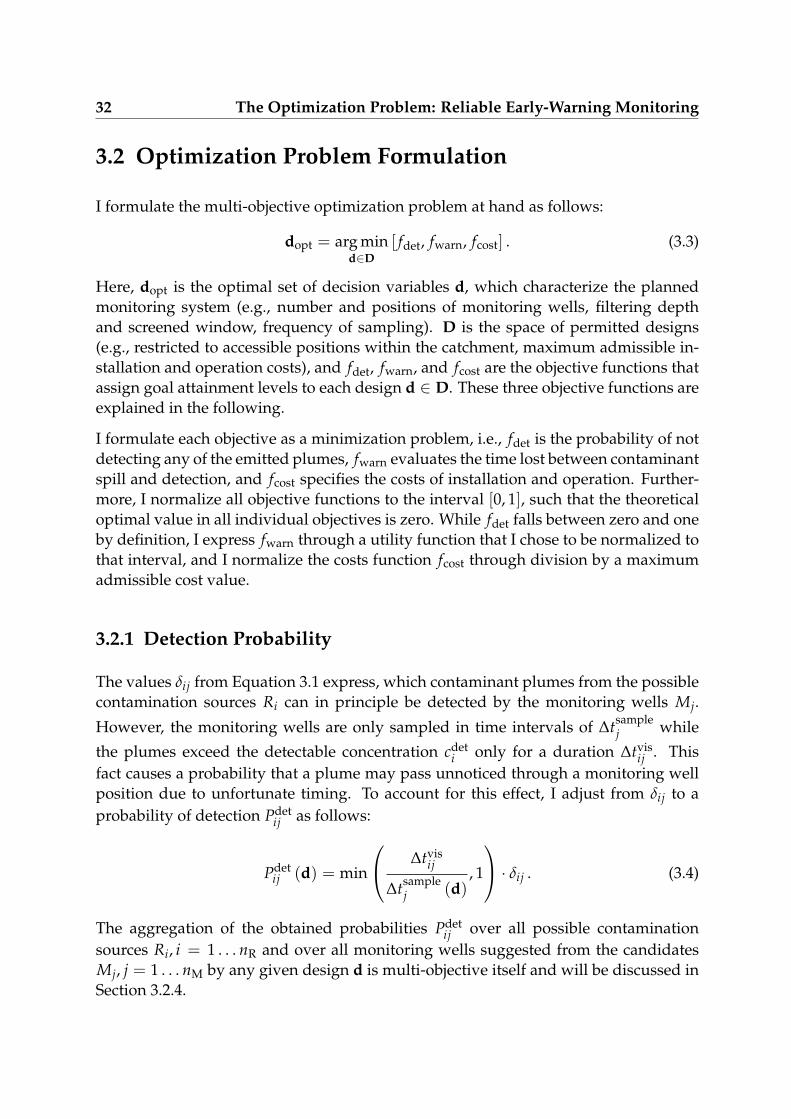
32 The Optimization Problem: Reliable Early-Warning Monitoring

3.2 Optimization Problem Formulation

I formulate the multi-objective optimization problem at hand as follows:

dopt = arg mind∈D

[ fdet, fwarn, fcost] . (3.3)

Here, dopt is the optimal set of decision variables d, which characterize the plannedmonitoring system (e.g., number and positions of monitoring wells, filtering depthand screened window, frequency of sampling). D is the space of permitted designs(e.g., restricted to accessible positions within the catchment, maximum admissible in-stallation and operation costs), and fdet, fwarn, and fcost are the objective functions thatassign goal attainment levels to each design d ∈ D. These three objective functions areexplained in the following.

I formulate each objective as a minimization problem, i.e., fdet is the probability of notdetecting any of the emitted plumes, fwarn evaluates the time lost between contaminantspill and detection, and fcost specifies the costs of installation and operation. Further-more, I normalize all objective functions to the interval [0, 1], such that the theoreticaloptimal value in all individual objectives is zero. While fdet falls between zero and oneby definition, I express fwarn through a utility function that I chose to be normalized tothat interval, and I normalize the costs function fcost through division by a maximumadmissible cost value.

3.2.1 Detection Probability

The values δij from Equation 3.1 express, which contaminant plumes from the possiblecontamination sources Ri can in principle be detected by the monitoring wells Mj.

However, the monitoring wells are only sampled in time intervals of ∆tsamplej while

the plumes exceed the detectable concentration cdeti only for a duration ∆tvis

ij . Thisfact causes a probability that a plume may pass unnoticed through a monitoring wellposition due to unfortunate timing. To account for this effect, I adjust from δij to aprobability of detection Pdet

ij as follows:

Pdetij (d) = min

∆tvisij

∆tsamplej (d)

, 1

· δij . (3.4)

The aggregation of the obtained probabilities Pdetij over all possible contamination

sources Ri, i = 1 . . . nR and over all monitoring wells suggested from the candidatesMj, j = 1 . . . nM by any given design d is multi-objective itself and will be discussed inSection 3.2.4.

3.2 Optimization Problem Formulation 33

3.2.2 Early-Warning Time

Early-warning time in context of supply-well protection is the time period betweenthe first detection of a groundwater contaminant and its arrival time at the productionwells. In other words, it is the remaining time for water suppliers to install coun-termeasures against the imminent contamination. Hence, a sufficiently long early-warning time for each possible contamination sources is desirable. Nonetheless, forthe optimization, a simple linear relation between individual early-warning time val-ues and the overall early-warning performance of a monitoring network is not suitable:the achievable early-warning time values for different possible contamination sourcesmay vary between none and several decades, and an increase in early-warning time ofremote sources is less valuable for water suppliers as an increase for close sources.

Therefore, I use a non-linear utility function Ui (t) (see Figure 3.1) for each possiblecontamination source Ri (illustrated by the different solid black lines). The utility Ui (t)is normalized by the individual maximum achievable early-warning time tmax

i that isdefined through the travel time τi,well from possible contamination source Ri to theproduction wells. A monitoring network that can achieve tmax

i as early-warning timeobtains a utility of one for source Ri. This specification serves to ensure that a monitor-ing well that achieves the maximum possible early-warning time for source Ri is ratedwith the maximum possible utility value.

Short early-warning times for supply-well contaminations are critical for a reliablefreshwater production and each increment of these early-warning times can be veryvaluable. Short early-warning times can either be related to possible contaminationsources close to the production wells or they are caused by a bad performance of themonitoring well. To distinguish these two scenarios, I introduce a user-defined mini-mum desirable early-warning time tmin and a corresponding early-warning time utilityumin that determines the benefit of tmin. tmin defines whether an early-warning time iscritical (orange and red area in Figure 3.1) and umin defines whether the performanceof a monitoring well is bad (red area in Figure 3.1). That is, the larger umin, the steeperUi

(t ≤ tmin

), and the larger the increase in utility for extended early-warning times to-

wards the maximum achievable early-warning time for possible contamination sourceRi. If the travel time τi,well is larger than a user-defined maximum desirable early-warning time tmax, tmax

i is set to tmax, such that longer early-warning times have noadditional benefit for the water supplier (green area in Figure 3.1). In other words,tmax is the maximum still useful early-warning time and monitoring wells within thegreen area provide maximum utility. The performances of monitoring wells withinthe yellow area in Figure 3.1 are between sufficient and very good. These monitoringwells can reach large early-warning times and high utility values. Usually, from tmin

to tmax, the utility should grow slower compared to the utility of the orange/red area.Early-warning times within this corridor still feature an increasing early-warning timeutility, but these extension are less important and can be seen as an extra benefit.

34 The Optimization Problem: Reliable Early-Warning Monitoring

Summarized, for remote possible contamination sources, monitoring wells should fallinto the green or the yellow area. Close possible contamination sources with shorttravel times towards the production wells should be monitored as early as possible(orange area). In either case, the red area should be avoided by monitoring wells.

Technically, I assign U(t = 0) = 0, U(t = tmin) = umin and U(t ≥ tmax) = 1. Thisyields as utility function:

Ui (t) =

1 ∀t : t ≥ tmax

(1−umin)·(t−tmaxi )

tmaxi −tmin + 1 ∀t : tmin ≤ t ≤ tmax

i ∧ tmaxi <

tmin

umin

ttmaxi

∀t : t ≤ tmin ∨ tmaxi ≥ tmin

umin .

(3.5)

Changes in all three user-defined values (umin, tmin, and tmax) might influence the finalresults more or less distinctively. For instance, umin defines the steepness of the utility-curve between 0 and tmin. Therefore, it can be seen as a catchment-specific weightingfactor for early or late detection, hence it needs to be chosen carefully.

3.2.3 Costs

The objective function for costs, fcost, is a summation of predefined and predictablecosts, like depth-specific drilling costs that are spatially variable, and operation costs

Absolute Early-Warning Time t

0 tmin

τi,well tmax

Utility

U(t)of

Early-W

arningTim

e

0

umin

1

1Figure 3.1: Case-specific utility function Ui(t) for early warning defined in Equa-tion 3.5. Each solid line represents the utility as a function of early-warning time ofpossible contamination sources that differ in τi,well. The colors represent four differentcharacteristic areas of this function.

3.2 Optimization Problem Formulation 35

that are composed of costs per sampling round within a given budget period:

fcost =NC

∑l

Cl , (3.6)

with NC different expenses Cl [AC]. Consequential costs are not included. Examples forconsequential costs are costs due to a shut down of production wells as consequence ofexceeding a threshold concentration, or high remediation costs due to a late detectionof a contamination and a large contaminated area. Since some consequential costs canbe extremely high, they are a strong motivation for installing reliable early-warningmonitoring networks. However, a consequential-cost function would complicate theoptimization problem dramatically and economic models would need to be added toforecast potential financial damages. These are two reasons why consequential costsare not considered in this work, but the extension would be technically straightfor-ward: they could be incorporated as separate objective functions without influencingany other implementations discussed here.

3.2.4 Evaluation of a Monitoring Network - Aggregation Rules

For any given design d, there is a list Ld of monitoring wells to be installed. From thatlist, several monitoring wells Mj, j ∈ Ld could have non-zero detection probabilitiesPdet

ij for any of the given possible contamination sources Ri. However, these monitoringwells could differ in early-warning time and detection probability, and we need to de-fine a rule how to identify a unique value for detection probability and early-warningutility for each possible contamination source Ri. We need such a rule to avoid thatthe monitoring wells have to be sampled for the whole list of possible contaminants(alternatively, this could also be solved by optimization).

There is no general rule that the monitoring well with the best early-warning time fora possible contamination source Ri will automatically have the best value in detectionprobability for this Ri. As a rule to identify a unique monitoring well per possiblecontamination source when rating the network performance, I use a method of bestcompromise. That means, I select the one monitoring well position Mj for the possiblecontamination source Ri out of the list Ld that maximizes the product of detectionprobability and early-warning time tij:

ℓi = arg maxj∈Ld

[Pdet

ij tij

]. (3.7)

Finally, I average the values of Pdetij with j = ℓi over all possible contamination sources

Ri to obtain the overall detection probability Pdetd of the monitoring network and de-

36 The Optimization Problem: Reliable Early-Warning Monitoring

fine:

fdet (d) = 1 − 1nR

nR

∑i=1

Pdetiℓi

︸ ︷︷ ︸Pdet

d

. (3.8)

As argued in Section 3.2.2, the achievable early-warning time values for different pos-sible contamination sources may vary between none and several decades, such that asimple linear relation between individual early-warning time values and the overallearly-warning performance of the monitoring network is not suitable. Instead, I workwith a non-linear utility function Ui

(tij

). Thus, in analogy to fdet, I define:

fwarn (d) = 1 − 1nR

nR

∑i=1

Ui

(tiℓi

)

︸ ︷︷ ︸Uwarn

d

, (3.9)

where Uwarnd is the overall early-warning utility of the monitoring network defined by

d.

3.3 Classification of the Optimization Problem

After formulating the optimization problem, it can be classified using the terms definedin Section 2.6. The optimization problem is based on a finite search space that containsall combinations of potential monitoring well locations (cf. Section 3.1), hence it is adiscrete combinatorial problem. The problem is high dimensional: each possible monitor-ing well location has the potential to influence the outcome of the optimization (at leastchanges in cost function). It is a multi-objective optimization problem with three compet-ing objectives with the objective functions defined above. The objective functions arehighly non-linear and the problem is very likely non-convex. The problem formulationis yet deterministic. However, it can easily be extended to a stochastic optimizationproblem (considering uncertainty), as I will present in the following section.

3.4 Considering Uncertainty for Reliable Monitoring

Networks

The objective functions fdet and fwarn use the simulation-based data specified in Sec-tion 3.1. Hence, they rely on model-based predictions about flow and transport inthe catchment, which are subject to uncertainty. The uncertainty arises from manysources, but I only focus on parameter uncertainty (as I discussed in Section 2.4),

3.5 Benchmark 37

which includes the description of flow boundary conditions. Uncertainty in transportboundary-conditions is already considered by the possible contamination sources.

When not accounting for uncertainty, the optimized monitoring network would mostlikely achieve a lower performance (when applied in practice) than predicted by theoptimization. Vice versa, accounting for uncertainty at least to some extent will makethe optimized monitoring networks robust against the considered parameter uncer-tainty.

Thus, I propose to perform Monte-Carlo simulations if the pdfs of the considered un-certain parameters are known, scenario analyses otherwise. Each scenario or Monte-Carlo realization k, k = 1, . . . , nk yields its own values δijk, τdet

ijk , τik,well and ∆tvisijk for the

quantities defined in Section 3.1. Then, we replace the affected objective functions fdet

and fwarn in Equation 3.3 by adequate statistics over the objective function values f(k)det

and f(k)warn obtained per realization:

dopt = arg mind∈D

[fdet, fwarn, fcost

], (3.10)

where f could denote, e.g., the largest value or a high percentile (since the objectivefunctions are formulated for a minimization problem) or the arithmetic mean. Theexpected value is a risk-neutral approach to optimization under uncertainty [e.g., 54],while working with extremes or percentiles is a risk-averse and even more robust ap-proach.

3.5 Benchmark

To demonstrate and discuss the proposed methods and approaches, I set up two syn-thetic application scenarios as test cases. The first test case is inspired by typical modelsused for well catchment management. It consists of a domain divided into a few zoneswith different hydraulic conductivity values. I will refer to it as Z_Based from now on,as zonation-based model. The second test case is abstracted from a real-world caseand captures key complexity of urban source water protection. Hence, I refer to it asU_Protect in the following, as urban water protection.

Both test cases represent a single geological layer of an aquifer as a quasi-three-dimensional domain (15,000m × 7,000m × 10m for Z_Based and 15,000m × 7,500m× 10m for U_Protect). The regional flow direction is approximately from east to west,defined through Dirichlet conditions at all domain boundaries. The prescribed bound-ary values follow geometrically from a uniform gradient that is specified through itsabsolute value and its orientation relative to the east-west axis. For simplification, allpossible contamination sources are assumed to be point sources with a pulse release of

38 The Optimization Problem: Reliable Early-Warning Monitoring

their contaminant. Each source is represented by 1000 particles released as point-likeand instantaneous injection (particles are injected within an area of 5 × 5 m2). In thefollowing, I describe both test cases in detail.

3.5.1 Z_Based

As mentioned above, the model domain of Z_Based is divided into several differenthydraulic conductivity zones with the intention to reflect typical groundwater modelsof water suppliers (e.g., developed with ModFlow). All relevant model parameters ofZ_Based are provided in Table 3.1, and a system sketch is shown in Figure 3.2. Nearthe eastern boundary of the model domain, there is a gallery of 15 pumping wells with50 meters spacing between neighboring wells. The figure also shows the location ofthe considered possible contamination sources as red circles.

For covering the robustness aspect mentioned in Section 3.4, Z_Based works with fourdifferent hydraulic scenarios (cf., Table 3.2) that differ in the strength of the regionalhead gradient, in its orientation angle, and in the overall pumping rate of the wellgallery. These scenarios represent aspects of hydrological uncertainty. They do notinclude the other sources of uncertainty listed in Section 2.4 to keep the applicationscenario straightforward. The different scenarios yield travel times from the most dis-tant possible contamination source to the well of up to 80 years. Again, for the sake ofsimplicity, I assume conservative tracer transport. This assumption may seem crude,but it is justifiable as a worst-case scenario for contaminant impact on the well, i.e.,unretarded transport and no degradation.

I discretize the domain with rectangular, equispaced cells sized 10m × 10m × 10mand simulate groundwater flow with the standard-Galerkin finite element code al-ready used in Nowak et al. (2008) [127]. For all subsequent transport simulations, Iemploy the Particle-Tracking Random Walk (PTRW) code used earlier by Enzenhoeferet al. (2014) [51] and by Koch and Nowak (2014) [90]. I choose PTRW due to its ease ofimplementation and its absence of numerical dispersion [e.g., 84, 102, 140].

Table 3.1: Transport-relevant parameters of Z_Based. The hydraulic conductivity valueprovided here is the arithmetic mean of all zone-wise values.

AverageconductivityK [m/s]

Porosityn [−]

Molecular diffu-sion coefficientDm

[m2/s

]Longitudinaldispersivityαℓ [m]

Transversedispersivityαt [m]

3.15 × 10−4 0.35 1 × 10−9 3 0.3

3.5 Benchmark 39

0 m 7 500 m 15 000 m0 m

3 500 m

7 000 m

10−4 10−3.5 10−3

hydraulic conductivity [m/s]

1

Figure 3.2: Model domain of Z_Based. Grayscale: zonation and values of hydraulicconductivity; Black rectangle: position of the well gallery; Blue overlay: union ofall scenario-wise well catchments (see Table 3.2); Red circles: possible contaminationsources.

Table 3.2: Definition of four different hydraulic scenarios

Hydraulic scenario Gradient strength [−] Gradient angle [] Pumping rate [l/s]

1 0.01 0 152 0.01 15 153 0.015 0 154 0.01 0 7.5

40 The Optimization Problem: Reliable Early-Warning Monitoring

3.5.2 U_Protect

U_Protect is a test case that captures the key complexity of a real-world case. It in-cludes:

• a random conductivity field instead of zonations,

• urban areas with a high density of possible contamination sources, and economicrestrictions in installation of monitoring wells and countermeasures, and

• inaccessible areas, where the feasibility of installing monitoring wells is notgiven.

The conductivity field is defined on a fine numerical mesh (10m × 10m × 10m) by Y =log (K). I assume local isotropy, that is, K simplifies to the scalar K. The field followsthe underlying discretized, two-dimensional multi-Gaussian random space function:

p (Y) ∝ exp(−1

2(Y − µY)

T C−1 (Y − µY)

), (3.11)

with Y as vector of Y-values at all locations within the domain. The random space func-tion is defined by the mean µY, the variance σ2

Y and a stationary covariance functionC (l) that is used to complete the covariance matrix C in Equation 3.11. As covariancemodel we use the Matérn covariance function [113]:

C (l) =σY

2κm−1Γ (κm)(2√

κml)κm Bκm (2

√κml) , (3.12)

with l as an effective separation distance between x1 and x2:

l =

√(∆x1

λ1

)2

+

(∆x2

λ2

)2

.

Here, Γ (·) is the Gamma function, Bκm (·) the modified Bessel function of the third kind[e.g., 1], κm is a shape parameter that controls the shape of the covariance function andλi with i = 1, 2 is the correlation length. All relevant model parameters of U_Protectare provided in Table 3.3, and a system sketch is shown in Figure 3.3.

On the eastern side at x = 13000 m, eleven pumping wells are installed, all along anorth-south line at y ∈ [3500, 4000] m, and each with a pumping rate of 30 l/s. Thedistance between neighboring pumping wells is 50 m. Within the test case there arethree different types of areas:

1. The open field with no limitation regarding the installation of monitoring wells(illustrated in Figure 3.3 as gray/white structure),

2. urban areas (illustrated in Figure 3.3 as maps) where it is not possible to installmonitoring wells, either because it is too expensive or because there are strongconflicts (e.g., mobility, shopping, ...), and

3.5 Benchmark 41

Table 3.3: Transport-relevant parameters of U_Protect. The hydraulic conductivityvalue provided here is the arithmetic mean of all values.

AverageconductivityK [m/s]

Porosityn [−]

Molecular diffu-sion coefficientDm

[m2/s

]Longitudinaldispersivityαℓ [m]

Transversedispersivityαt [m]

0.08 0.3 1 × 10−9 1 0.1

3. inaccessible areas (illustrated in Figure 3.3 as a forest) where it is not possible toinstall monitoring wells, because it is too expensive in time, effort and costs.

For representing uncertainty in hydro(geo)logy, I vary (a) the ambient flow directionof the groundwater, and (b) the conductivity field. The variations in ambient flowdirection are controlled by the Dirichlet boundary condition: the general flow direction

is corrected by an angle β drawn from a normal distribution N(

µβ, σ2β

)with mean

µβ = 0 and variance σ2β = 102.

0 m 7 500 m 15 000 m0 m

3 750 m

7 500 m

10−5 10−3 10−1

hydraulic conductivity [m/s]

1

Figure 3.3: Model domain of U_Protect. Grayscale: values of hydraulic conductivity;Black rectangle: position of the well gallery; Maps: urban areas; Forest: difficult acces-sible area; Red circles: possible contamination sources within urban areas.

42 The Optimization Problem: Reliable Early-Warning Monitoring

The variations in the conductivity field are controlled by the covariance functionC (l) (Equation 3.12). Following the Bayesian geostatistical approach [e.g., 87], alsothe covariance function is uncertain. Therefore, I model the structural parametersθ =

[σ2

Y, λi, κm]

as random variables and the covariance function C (l) itself becomes arandom function governed by the random parameter θ: C (l, θ).

3.6 Exemplary Results

In this section, I exemplary discuss an optimization result of the optimization problemdefined above. Therefore, I use optimization outcomes from the following Chapter 4,where all relevant optimization settings can be found in Table 4.4. I discuss the resultsusing Figure 3.4 and Figure 3.5.

Figure 3.4 shows an approximation of the Pareto front of the optimization problem(red spheres) and the projections of the three-dimensional approximation set ontothe planes of the coordinate system. Figure 3.5 shows two different monitoring net-works for U_Protect. One is marked with black crosses and the other one is markedwith green pluses. In the following discussion, I refer to the networks as CROSSESand PLUSES. The two selected monitoring networks CROSSES and PLUSES are high-lighted as green and black spheres, respectively, in Figure 3.4, according to their colorsin Figure 3.5.

Figure 3.4 clearly reveals that the three considered objectives are competing. One canachieve a full coverage of all possible contamination sources at maximum early warn-ing utility, but only with a budget that allows installing 9 monitoring wells (blacksphere of the approximation set). At decreasing costs, one can either maintain max-imum detection probability (back/right edge of the approximation set) while losingearly-warning time, or one can try to lose less early-warning functionality but restrictthat functionality to a smaller number of possible contamination sources (back/leftedge of the approximation set). In general, for this problem there is a list of four ge-ometric aspects in the Pareto front (and approximation sets) that will hold for anycatchment:

1. The idealistic goal of benefits without costs (blue sphere in Figure 3.4) can neverbe reached.

2. Maximum detection probability and yet minimum costs are only possible bydirectly monitoring the mixed water of the pumping-well gallery (bottomfront/right corner of the objective space). Since I did not consider this case asrelevant in our application, the optimization was not forced to search for Paretooptima at this part of the approximation set.

3.6 Exemplary Results 43

Normalized

Costs

[-]

0

0.5

1

Detection Probability [-]1

0.5

0

Benefit

ofEW

T[-]

1

0.5

0

1

Figure 3.4: Approximation of the Pareto front for the multi-objective optimizationproblem on U_Protect. Blue sphere: theoretical optimum; Red spheres: non-dominated solutions (approximation set of the Pareto front); green and black sphere:performance of the selected monitoring networks shown in Figure 3.5 (green: PLUSES;black: CROSSES). Gray dots projections of the approximation set onto the planes of thecoordinate system

44 The Optimization Problem: Reliable Early-Warning Monitoring

3. The solution with almost no costs and a very poor detection of the possible con-tamination sources (bottom/left edge of the objective space) is to place one indi-vidual monitoring well at the cheapest individual drilling position and dependsonly on the complexity of fcost. This selection defines the bottom back/bottomleft tip of the Pareto front.

4. The top/right back tip of the Pareto front is given by the most expensive solutionthat places monitoring wells close to the possible contamination sources.

These four facts define the fundamental geometry of the Pareto front. Only the cur-vature of the Pareto front towards the idealistic unattainable optimum depends onthe properties of the investigated catchment and the positions of its possible contam-ination sources. Contamination sources arranged in a line transverse to the dominantflow direction would lead to a strong competition between the objective functions (andhence to a low curvature of the Pareto front) because non-overlapping plumes prohibitthe monitoring of several possible contamination sources with only a few monitor-ing wells. Possible contamination sources arranged in a longitudinal line would leadto one overlapping plume, with almost no competition between costs and detection.Clustered possible contamination sources would fully remove the competing characterof all objective functions because these sources could be monitored with good early-warning time by just one or a few monitoring wells very close to the spill location.

The selected monitoring networks shown in Figure 3.5 both have a detection proba-bility of 100%, i.e., they reliably monitor all possible contamination sources. However,they starkly differ in their number of monitoring wells (9 for CROSSES, 5 for PLUSES),and hence in costs (88% vs. 41% of maximum costs). The high performance of PLUSESin detection probability at relatively low costs can be achieved by the strategy to mon-itor the well catchment at positions where several predicted contaminant plumes co-incide. As a result, the network PLUSES is shifted towards the pumping wells, andfurther away from the possible contamination sources. In contrast, the more expensivenetwork CROSSES forms a barrier wall close to the urban areas, where all possiblecontamination sources occur. Consequently, the performance in early-warning time ofCROSSES outperforms the one of PLUSES.

3.6 Exemplary Results 45

0 m 7 500 m 15 000 m

0 m

3 750 m

7 500 m

1

Figure 3.5: Model domain of U_Protect (cf. Figure 3.3). Grayscale: values of veloc-ity field; Magenta overlay: possible contamination plumes (degree of transparency isequivalent to the number of overlapped plumes); Black crosses/green pluses: possiblemonitoring networks.

Chapter 4

Representation and Reduction of theSearch Space

This chapter is based on the submitted manuscript Search Space Representation and Re-

duction Methods to Enhance Multi-Objective Water Supply Monitoring Design to the Jour-nal WATER RESOURCES RESEARCH [21]. I am reusing parts of the text and figures fromthis manuscript.

This chapter builds on the general problem formulation from the previous chapter.It contributes enhanced approaches for managing large search spaces to make opti-mization faster (computationally less expensive) without sacrificing the quality of theattained trade-off solutions. These methods work for combinatorial optimization prob-lems with a precalculable search space and approach the problem of speed by reduc-ing or re-organizing the search space. Fortunately, my problem formulation allows forprecalculating the transport simulations for each possible contamination source andmonitoring well such that the mathematical space of possible monitoring-well posi-tions and a few relevant properties are known before searching for optimal monitoringnetworks. From this available information, all possible monitoring networks can becreated, hence the search space is precalculable. The strategies introduced in this chap-ter focus on two key aspects of the design problem:

1. a more compact representation of the search space that can be addressed withevolutionary multi-objective search operators, and

2. a formal mathematical screening of candidate decisions to reduce the searchspace.

While the representation of the search space affects the optimization algorithm in use,the search-space reduction is a pre-processing step with a stand-alone application.Both general ideas are outlined in the following two paragraphs.

Representation of the search space. We assume that the optimization is based onprecalculated numerical transport simulations from all possible contamination sourcestowards the production wells. Then, we have a discrete approximation of our modeldomain (the well catchment) and a finite set of possible monitoring-well positions. The

47

search space consists of the power set of all possible monitoring-well positions, henceits size can easily reach intractable dimensions. For instance, the number of possi-ble monitoring networks with up to 15 monitoring wells arranged from 100 possiblemonitoring-well positions yields a search space larger than 3 × 1017 possible combi-nations (without repetition). Therefore, usually, the search space (power set) is notdefined explicitly, but implicitly by all possible monitoring-well positions. The set ofall possible positions can reproduce all combinations the search space contains. Forthe sake of generality, I use the term elementary decision options or EDOs to refer tocandidate monitoring-well positions, and the EDO set to define the entire mathemat-ical space of all possible monitoring-well positions. A common representation of theEDO set during the optimization is the binary representation (cf. Section 4.2.1). How-ever, state-of-the-art evolutionary multi-objective algorithms struggle with the binaryrepresentation in combination with large EDO sets that have complex interdependentdecision variable sensitivities on the objective functions [95, 146]. The number of dis-crete decision variables directly correlates with the total number of EDOs (NEDO) aswell as with the computational scaling of the search tool [94]. To reduce the numberof decision variables, I introduce the linear-indexing representation in Section 4.2.2 thatis based on the random keys representation proposed by Bean (1994) [6]. The basic ideaof the random keys representation is that the search for optimal solutions takes placeon an easier surrogate space that is more appropriate to the translation and variationoperators of heuristic optimizers than the original (binary) mathematical space. Thelinear-indexing representation underlies the random keys representation and serves todecouple the number of decision variables from the exponential growth of the powerset of EDOs.

Reduction of the search space. Evolutionary multi-objective optimization representsa balance between robustness to challenging mathematical problem features (noncon-vexity, discreteness, stochasticity, nonlinearity, etc.) and the degree to which the algo-rithms maintain their ability to provide high-quality Pareto-approximation sets. A corecontrol on this balance is the number and type of decisions that compose the searchspace. A common strategy to more effectively address this balance is to reduce thesearch-space size. A number of different reduction strategies have been established inthe literature. An overview of existing methods can be found in the position paper ofMaier et al. (2014) [109]. Many of these methods use adaptively refining grids, eitheron binary encoding [e.g., 64, 144, 175], or numerical grid-based dynamic emulation[e.g., 5, 148]. Alternatively, Walters and Lohbeck (1993) [170], as well as Walters andSmith (1995) [171], focus on screening solutions that are not valid or feasible. Build-ing on a similar logic, I propose decision space reduction strategies that exclude EDOs(along with large portions of the search space in the corresponding power set) that arelimited in their influence on the optimization. Simple exclusions are already possiblegiven expert knowledge about the optimization problem. For example, in ground-

48 Representation and Reduction of the Search Space

water monitoring, one could remove candidate monitoring wells where it would beimpossible to detect contamination. Usually, the expert-driven reduction of the set ofEDOs yields a search space that still remains very large. Further reduction can be doneby excluding redundant EDOs from the set. The check for redundancy is based oncomparing pairs of EDOs. If one EDO dominates the other or both are equally good,the better option remains in the set, and the other one can be excluded. There aredifferent approaches for implementing this comparison. It can be done in a system-atic manner (e.g., all EDOs are compared among each other), or it can be done with aheuristic, randomized screening method.

As the overall optimization problem of this thesis is combinatorial, a reduction of sin-gle possible monitoring-well positions would reduce the number of their combinationsdramatically. For instance, a relatively small problem with an EDO set of 100 possiblemonitoring-well positions and a search space that includes combinations of 1 to 5 mon-itoring wells, can be simplified by more than 40% when 10 positions of the EDO set areproven to be irrelevant and removed (from ∼ 79 × 106 to ∼ 47 × 106 possible solu-tions). That is, the optimization algorithm can either search more intensely within theremaining 60% candidate solutions for optimal solutions, or it can keep the intensitylevel, but reduce optimization time.

The presented representation and reduction methods in this chapter significantly en-hance the effectiveness, efficiency, and reliability of the optimization. The proposedframework shifts focus to the most impactful monitoring design decisions while alsoenhancing decision makers understanding of key performance trade-offs. In combina-tion, the proposed representation and reduction techniques have significant promisefor enhancing the size and the scope of combinatorial monitoring problems that can beexplored.

The remainder of this chapter provides a more detailed explanation of our proposedrepresentation and reduction contributions. The following section introduces the usedoptimization algorithm (the Borg MOEA [69]) and its performance metrics. Section 4.2describes the different ways in which the search space within the optimization wasrepresented. In Section 4.3, I define the reduction strategies explored in this study.Here, I also generalize the methods to show that they can be used for a broad classof optimization problems. I provide a list of conditions that a problem has to meetto reliably speed up and to improve the optimization procedure with our reductionmethods. Section 4.4 provides the details of the computational experiment used tobenchmark the contributions. Section 4.5 presents the results and discussion of thetested search space representation and reduction methods. Finally, in the last section(Section 4.6), I summarize and conclude this study.

4.1 Methods 49

4.1 Methods

4.1.1 Multi-Objective Optimization Algorithm

Reed et al. (2013) [134] showed that the Borg MOEA [introduced in 69] has competi-tive to superior performance relative to existing state-of-the-art MOEAs on a diversesuite of multi-objective water resource applications including a monitoring benchmarkproblem. These results motivated my use of the Borg MOEA. The key characteristicsof the Borg MOEA are:

1. the use of an ǫ-dominance archive [103] that enhances the convergence and thediversity of the approximation set,

2. the use of ǫ-progress [69] to evaluate the search progress and to avoid stagnationin search,

3. the adaptive re-sizing of the population [75, 93] to provide a population largeenough to improve the current approximation set but small enough to still beefficient in calculation time,

4. the adaptive selection of multiple recombination operators [168], based on thecurrent solution-composition of the approximation set and

5. that Borg is a steady-state ǫ-MOEA [35] that avoids computationally expensiveoperations and can be easily parallelized.

Borg includes six different recombination operators: Simulated Binary Crossover (SBX)[32], Differential Evolution (DE) [155], Parent-Centric Crossover (PCX) [34], SimplexCrossover (SPX) [162], Unimodal Normal Distribution Crossover (UNDX) [86], andUniform Mutation (UM). Additionally, Polynomial Mutation (PM) [32] mutates theoffsprings generated by SBX, DE, PCX, and SPX.

4.1.2 Performance Metrics

I use the normalized hypervolume as the performance metric, where the hypervol-ume of an approximation set is normalized by the hypervolume of the reference set(cf. Section 2.7). The hypervolume is a good indicator of the proximity and diversityof attained approximation sets. Achieving hypervolumes close to one signals that theapproximation set is meeting the same level of diversity and proximity as the referenceset. Hypervolume also provides a rigorous means of ranking alternative problem for-mulations regarding their performance. Overall, we can evaluate MOEA performancein terms of effectiveness, efficiency, and reliability. An effective optimization means that

50 Representation and Reduction of the Search Space

the hypervolume of an approximation set is close to one. Efficiency describes the abil-ity of the search algorithm to quickly find good solutions, which can be measured bythe number of function evaluations (NFE) or the optimization runtime necessary fora specific hypervolume attainment. Reliability refers to minimizing the variation inattained search results across random-seed trials. For calculating the hypervolume, Iuse the diagnostic framework of Hadka and Reed (2012) [68].

4.2 Representation of Search Spaces

When tackling an optimization problem with an MOEA, algorithmic representation ofthe search space is fundamentally important as it shapes the scope of search as well asthe appropriateness of search operators (i.e., mating, mutation, and selection). Here,I only discuss spatially discretized problems as illustrated in Figure 4.1. Again, thesearch space is implicitly defined via an EDO set that contains all elementary deci-sion options, while the explicit definition would be the power set of all EDOs (i.e., allpossible combinations of the elementary decision options).

Solutions within the search space can be addressed in different ways that directlydepend on the representation of the EDO set. In many optimization problems, it isappropriate to represent the search space by the physical meaning of the EDOs di-rectly (in the current problem the physical meaning are the coordinates of the possiblemonitoring-well positions). However, the EDO-set representation is required to beclosed under the genetic operators of the optimization algorithm. That is, when thegenetic operators are applied to EDOs, the resulting elements should be EDOs as well,hence a part of the EDO set. Otherwise, the genetic operators could generate invalidsolutions.

Figure 4.2 shows the meaningful physical EDO set of U_Protect (see Section 3.5.2) asgray area on the bottom plane. It is obvious that this EDO set is not closed againstthe genetic operators when using coordinates to represent the search space becausethe genetic operators could easily enter invalid (not gray) areas. A possible closingstrategy is to make the search area convex by overestimating it to include the voidspace (in Figure 4.2 the interspersed white spaces between gray areas in the bottomrectangle). However, the complexity of the optimization problem would increase un-necessarily and the search would be likely to degrade in effectiveness and efficiency.Thus, I present two different representation approaches in the following two sections.

4.2.1 Binary Representation

The binary representation of search spaces is often used in discrete optimization prob-lems [e.g., 135] and many optimization algorithms are preset for a binary optimization

4.2 Representation of Search Spaces 51

OnOff

Set of

EDOs

...1 2 3 3635343332 37

Real Physical Space

EDOs

1

Figure 4.1: Basic steps to represent the search space in the current test case (from leftto right). First, the physical space is approximated by numerical simulation. The set ofEDOs is given by the mesh discretization and implicitly defines the search space. Sec-ond, with binary representation, all EDOs are decision variables and switch betweentwo statuses: on or off. That is, only activated decision variables determine the out-come of the solution. Third, with linear-indexing representation, the set of EDOs (herein total 37 EDOs) is reshaped to a list. The number of decision variables is indepen-dent of the number of EDOs and only depends on the desired maximum number ofmonitoring wells.

(e.g., traditional genetic algorithms [174]). This representation follows the criteria ofclosure through the use of integer operators such as rounding because all EDOs canonly be zero or one (EDO ∈ [0, 1]). Especially for combinatorial problems, the binaryrepresentation is intuitive. For instance, consider the optimal design of monitoring net-works: a monitoring-well position can be switched on or off and the MOEA is search-ing for the best on/off combinations (cf. middle sub-figure in Figure 4.1). That is, eachsolution is a list of on/off decisions and contains the entire set of EDOs, all decisionvariables, respectively.

Although the binary character of the decision variables appears simple, this rep-resentation is limited to problems with a relatively small number of decision vari-ables (< 200) on currently available machines. The presence of fiscal constraints andphysics-based interdependencies between the binary decisions makes the monitoringproblem an extremely difficult analog to the classic combinatorial Knapsack (i.e., withnon-deterministic polynomial time hardness or NP-hard [95, 146]).

4.2.2 Linear-Indexing Representation

As a means of reducing the number of decision variables and to better manage prob-lems with a large number of EDOs, I introduce the linear-indexing representation of thesearch space. For a discrete problem, the set of EDOs can be transformed into a listLid of linear indices that just contain the information about the original location of theEDOs within the EDO set (cf. right sub-figure in Figure 4.1). The approach is to ad-dress the list Lid via an index i (i ∈ E and E = 1, 2, . . . , NEDO) and use the linear

52 Representation and Reduction of the Search Space

set E as a surrogate for the actual EDO set. With that, the index i becomes a decisionvariable and the number of considered decision variables is limited by the user to themaximum number of EDOs (Nmax) per solution (e.g., a maximum number of monitor-ing wells given by an upper-cost constraint). We complete our set of decision variableswith a set of binary decision variables that define whether a drawn EDO (via the indexi) is part of the solution candidate or not. With this, we achieve that the number ofdecision variables is constant, even if a solution addresses less than the number Nmax

of EDOs. We can guarantee the closure of the EDO set under the genetic operators bythe use of integer operators for both types of decision variables. For a combinatorialoptimization problem, linear-indexing representation reduces the number of decisionvariables dramatically compared to the binary representation, if the maximum desirednumber of decision variables Nmax is small compared to the EDO set. For instance, ifthe upper limit of a planned monitoring network is five wells, only ten decision vari-ables are required: five that address the actual locations of the monitoring wells andanother five that switch the five drawn monitoring wells on or off.

For efficient and effective optimization runs, the sorting of the EDOs within the listLid is crucial. This is because, when using evolutionary algorithms, proximity in thesearch space should imply proximity in the objective space. In Figure 4.2 the EDO setof U_Protect is illustrated. Here, the gray area on the lower plane illustrates the binaryrepresentation. The colored area with the gradient from upper back to lower frontillustrates the linear-indexing representation. The values on the z-axis represent theposition of the EDOs within Lid. All EDOs are sorted by their distance to the pumpingwells. Thus, neighboring EDOs within the EDO set that might have similar charac-teristics, are also contiguous within Lid. A more advanced sorting strategy that workswithout educated guess about the properties of the problem could sort the EDOs di-rectly based on similarity characteristics in the objective space, e.g., using clusteringvia a k-means algorithm [76], or according to travel times ( fwarn) from/to sources orwells.

4.3 Search Space Reduction Methods

In the following sections, we discuss possible reduction methods for precalculated,finite, and discrete search spaces. We explore reduction methods with a range of prop-erties including ease of implementation, strength of reduction, and preservation ofPareto-optimal solutions. The three reductions are summarized as follows:

1. The fundamental reduction method requires knowledge about the optimizationproblem and about the numerical-model results that provide the pre-calculateddata for the optimization. This method removes obviously irrelevant EDOs fromthe EDO set.

4.3 Search Space Reduction Methods 53

NEDOs

0 m

7 500 m

15 000 m 0 m3 500 m

7 000 m

Linear-IndexingRepresentation

BinaryRepresentation

1

Figure 4.2: Example of the two discussed methods how to represent the search space.The binary representation is illustrated as a gray area where a contamination can bedetected. The linear-indexing representation is illustrated as colored surface. The z-values describes the position within the list of all EDOs (i.e., it corresponds to thesorting of the EDOs). Thus, the sorting can influence the efficiency of the optimizationand can be done in different ways. In this illustration, the EDOs are sorted by theirdistance to the pumping wells.

2. The grid-based reduction method is often used for optimization problems and iseasy to handle. It discretizes the EDO set using a grid and represents all EDOswithin the same grid cell by the best single EDO that is determined by user-defined rules.

3. The comparison-based reduction method compares the goal attainment of two arbi-trary EDOs and removes the dominated one. We present two different imple-mentations, the optimal reduction, and the optimization-based reduction.

Their key characteristics are summarized in Table 4.1.

4.3.1 Fundamental Reduction

The search space for many optimization problems has a high potential for simple andfast reduction. Reduction can be considered at two fundamental levels.

First, external constraints can be used to a priori screen out EDOs that are not favorable.For example, in the U_Protect test case (cf. Section 3.5), all monitoring-well positionsthat trigger high installation and/or operation costs, can be excluded, also when thereis a dangerous or infeasible installation of a monitoring well (e.g., in cities, or anhydrite

54 Representation and Reduction of the Search Space

Table 4.1: Key Characteristics of the Presented Reduction Methods

Reduction Method Easy to implement Reduction poten-tial

Possible loss ofPareto-optimalsolutions

Fundamental Yes Varies NoGrid-Based Yes High YesOptimal No Varies NoOptimization-Based

No High Yes

layers that could grow when coming into contact with water). These areas are shownas maps or forest in Figure 3.5. When doing this reduction too generously, there is arisk of over-restricting the EDOs and eliminating important decision alternatives fromthe search space. Strong restrictions within the search space might lead to the lossof solutions that would otherwise be part of the Pareto-optimal set. That being said,extremely large decision spaces with complex constraints could require dramaticallymore search or even render search operators invalid.

Second, for precalculated problems, the meaningful set of useful EDOs can be deter-mined a priori and the search is restricted to the useful EDOs. In our case, the pre-calculated dataset clearly identifies all positions where a contamination could be de-tected, and those where no contaminant plume from any of the possible contaminationsources will ever pass by. That is, using the complete model domain as the EDO setis pointless, because many of its EDOs only cause costs but do not contribute to amonitoring-network solution. These useless EDOs can be excluded easily and quicklyfrom the EDO set without the risk of losing relevant Pareto-optimal solutions from thesearch space. This reduction leads to the fingered geometry of the remaining EDOpositions in Figure 4.2, also shown in Figure 3.5 as semi-transparent red areas down-gradient of the considered possible contamination sources.

4.3.2 Grid-Based Reduction

The basic idea of the grid-based reduction is to represent the actual EDO set by a re-duced set of representative EDOs. The choice of the representative EDOs is based ona regular or irregular coarse-meshed grid that more coarsely discretizes the originalEDO set. Then, all EDOs within a discretization element of the coarse grid are repre-sented by just one EDO. Optimization problems that are strongly focused on a spatialEDO set frequently employ this reduction method [e.g., 5, 96, 105]. The main drawbackis that potentially well-performing EDOs get lost that could better contribute to globalsolutions than their representative EDOs. There is no guarantee that the lost EDOs

4.3 Search Space Reduction Methods 55

are not part of any Pareto-optimal solution. However, this method is a very effectivereduction method and easy to implement.

Here, I implemented this reduction method on U_Protect and used a grid resolutionthat was coarse enough to downsize the EDO set such that the binary representationcould be applied. I used three decision criteria to find the representative EDOs:

1. all EDOs that could only detect one possible contamination source were directlyremoved,

2. in each discretization element, among all remaining EDOs, I kept only theone that could detect the largest number of up-gradient possible contaminationsources, and

3. in the case that two locations could monitor the same number of possible con-tamination sources, I kept the EDO that was closer to the center of area of alldetectable plumes.

I did not use the early-warning time as a third decision criterion because, within onediscretization element, the differences of the EDOs are relatively small compared to theoverall travel time of the contaminants to the production wells.

4.3.3 Comparison-Based Reduction Methods

While the grid-based reduction method is a brute-force method that eliminates EDOswithout checking whether any EDO might be part of Pareto-optimal solutions, thefollowing two comparison-based reduction methods identify only irrelevant EDOs andexclude them from the EDO set.

The main idea is to check, whether a single EDO xj can either be replaced by anotherEDO xk because they have the same effect or because EDO xk dominates EDO xj. Forthe check whether EDO xj can be excluded from the EDO set or not, all objective valuesfi (x) (with i = 1, 2, . . . , NOF and NOF as the number of objective functions) must fulfillthe following three conditions:

1) f (xk) f(

xj

)and (4.1)

2) f (xk) f(

xj, xk

)and

3) f (X) f(xj, X

)or f (xk, X) f

(xj, X

).

Here, f denotes the set of objective functions fi and X is an arbitrary subset of EDOswithout xj,k

(X ⊆ EDO set\

xj, xk

). In detail, Equation 4.1 means:

56 Representation and Reduction of the Search Space

1. If EDO xk is not dominated by EDO xj (described by ), and

2. xk is also not dominated by the set of both EDOs[xj, xk

], and

3. if any arbitrary EDO subset X is not dominated by the set[xj, X

], or if the set

[xk, X] is not dominated by the set[xj, X

], then xj can be removed from the EDO

set.

In the case when all three constraints are fulfilled, the EDO xj cannot be a part of anyPareto-optimal solution, because the gain in goal attainment will always be higher withxk for any solution.

While the first and the second constraints in Equation 4.1 are intuitive, the third con-straint is just for completeness. Many objective functions already include the third con-straint if the first and the second are fulfilled (e.g., all monotonic objective functions).If the third constraint must be evaluated for each comparison step, the comparison-based methods are not feasible anymore, because the number of all arbitrary subsets X

is almost as large as the explicit search space.

Comparison-based methods only work in a meaningful manner for discretized prob-lems and finite EDO sets. Otherwise, they would suffer infinite runtime. In the follow-ing, I will present two different methods that use the EDO-comparison concept: the op-

timal reduction method and the optimization-based reduction method. The main differencebetween the two methods is that the optimal reduction method globally and systemati-cally identifies all irrelevant EDOs, and the optimization-based reduction method onlychecks the relevance of EDOs relative to already checked EDOs. Unchecked EDOs can-not be a part of the resulting reduced EDO set. In other words, for the first method,it can be guaranteed that no EDO will be excluded that is part of a Pareto-optimal so-lution set, while for the second method it can only be guaranteed that the remainingEDOs are better than the checked and excluded EDOs. However, there might be betterEDOs within the unchecked but excluded EDOs.

Optimal Reduction

As already said above, the optimal reduction method uses the EDO comparison glob-ally. The degree of EDO-set reduction and the runtime of this method depends on thecharacteristic of the EDO set. Two characteristics are of special relevance: (1) the spatialvariability of similar EDOs, and (2) the variability of objective values of all EDOs:

1. EDO sets with many spatially clustered redundant EDOs can significantly be re-duced in relatively short time.

2. EDO sets with highly variable EDOs in objective values cannot be reducedstrongly, because the EDOs can cooperatively complete their individual weak-nesses.

4.3 Search Space Reduction Methods 57

3. EDO sets with many redundant EDOs that are spatially variable would lead toa long runtime because the ratio of comparison operations and eliminations ofEDOs would clearly be on the side of comparison operations.

While the first case is ideal from the view of reduction, the second and the third casesare suboptimal. However, at least for the third case, it is possible to shift the ratiobetween comparison operations and eliminations of EDOs to the elimination side. Fol-lowing the first characteristic from above, the order of comparison is crucial for com-putational efficiency. For example, the probability that two potential monitoring wellsM1 and M2 monitor the same possible contamination sources is high when M1 and M2

are neighbors. Then, M1 might be dominated by M2 (or vice versa) and together theymight not provide any improvements; M1 can be excluded from the EDO set. If M1 isnot contiguous to M2 and they monitor different possible contamination sources, to-gether they always improve the overall objective value for detection probability. Whenacknowledging this behavior, for the third case the organization of EDOs can be ma-nipulated regarding their objective values such that clusters of similar EDOs are neigh-boring upon re-organization. Alternatively, all EDOs can be sorted according to theirdistance to the current reference EDO (cf. Figure 4.2) to identify clusters of similarEDOs.

A special case of EDO sets with highly variable EDOs in the objective space (secondcase) is an EDO set with a small value range. Many EDOs provide almost the samequality, but cannot be removed from the EDO set following the rules defined in Equa-tion 4.1. Then, an effective computational efficiency booster for the optimal-reductionmethod is to modify the objective space of the fundamental EDO set in a way thatEDOs with different, but almost equal, qualities are getting the same values (called be-

ing homogenized in the following). This approach reduces the number of EDOs withinthe comparison steps (cf. Equation 4.1). More EDOs can be rejected immediately be-cause only one of multiple EDOs with the same quality (after the homogenization)must be a part of the final reduced EDO set. For the homogenization of the funda-mental EDO set, we discretize its objective space in hyperboxes with a side length ǫ

similar to the ǫ-box dominance concept (cf. Section 2.6.2). Then, we can either applythe ǫ-box dominance concept and only accept a single non-dominated solution per hy-perbox, or we randomly choose a solution per box (equivalent to the round function).The difference between the two methods is illustrated in Figure 4.3. With an increasingdiscretization length ǫ, the EDO set would be more homogeneous in objective values,and the reduction would be more efficient. However, both approaches (ǫ-box conceptand round-function) would nullify the guarantee that the reduced EDO set containsall Pareto-optimal solutions. Still, but depending on the discretization length ǫ, theresulting EDO sets could be a very good approximation of the optimal reduced EDOset. Therefore, I suggest applying these methods only if the EDO set is very indifferentin the objective values of the EDOs, such that a combination of two EDOs has almostno impact on the joint objective value.

58 Representation and Reduction of the Search Space

OF1

OF2

1

Figure 4.3: Differences between the ǫ-box dominance concept and the round function(colored boxes discretize the objective space) on an example with the two objectivefunctions OF1 and OF2. The red line illustrates the real but unknown Pareto front. Thedots are candidate solutions. Each box is represented by one solution that becomesselected over multiple other candidate solutions per box (black dots). The differencebetween the ǫ-box dominance concept and the round function is that the ǫ candidatesare deterministically selected out of all non-dominated box solutions (green and blackdots, the gray dots are dominated) and the round function handles all candidate solu-tions within a box equally and also dominated solutions can be selected.

Optimization-Based Reduction

The optimization-based reduction method uses formal optimization algorithms to approx-imate the EDO set of the optimal reduction method introduced directly above, henceis an alternative but an approximate approach for complex and large EDO sets. Therequired optimization algorithm for the reduction can be the same as for the entire op-timization problem. However, it might be necessary to adopt the objective functionsof the overall problem, if the objective functions aggregate over multiple single values.With the aggregation, information will be lost and EDOs will be wrongly excludedfrom the EDO set. For instance, in Equation 4.2 two EDOs are being compared bythe aggregating objective function f∗. Although the single values of both EDOs differ,they have the same aggregated objective value ( f 1

∗ and f 2∗ ) and together, they would

increase the aggregated objective value:

4.4 Computational Experiment 59

f 1∗ = mean

(10

)= 0.5

f 2∗ = mean

(01

)= 0.5 (4.2)

f 1,2∗ = mean

(11

)= 1.

Therefore, when working with aggregating objective functions, the comparison musttake place on the non-aggregated level, such that only EDOs are eliminated if all singlevalues are dominated by another EDO.

The objective functions of our optimization problem aggregate over the single valuesfor all possible contamination sources. However, to evaluate the performance of mon-itoring wells, it also matters, which possible contamination source they are able tomonitor. That means, we have to segregate our objective functions into objective func-tions for each possible contamination source. This modification leads to an increase indimensionality of the optimization problem, but the segregated objective functions areeasy to evaluate.

Although the approximation of the optimal reduced EDO set can save computing time,there are two drawbacks compared to the optimal reduction of the EDO set: (1) itis an approximation, thus EDOs might be excluded from the EDO set that could bepart of a Pareto-optimal solution, and (2) the quality of the EDO set depends on theruntime of this pre-optimization, generating yet another trade-off between efficiencyand effectiveness.

4.4 Computational Experiment

The computational experiment exploits the U_Protect test case described in Section 3.5with and without considering uncertainty. The U_Protect benchmarking problem cap-tures key source water protection monitoring challenges as to contribute generalizableinsights when distinguishing our proposed approaches for reduction and representa-tion of the search space.

Without considering uncertainty First, I simulated the contaminant evolution fromall 30 possible contamination sources towards the pumping well (using the particle-tracking-random-walk method) and recorded all relevant data that were needed forthe objective function (cf. Section 3.2). Second, on the resulting set of EDOs, I applied

60 Representation and Reduction of the Search Space

the fundamental reduction (Section 4.3.1) to get the base EDO set. Third, on this baseset, I tested the remaining reduction methods introduced in Section 4.3. Then, I for-mulated seven different problem formulations varying the different EDO sets and therepresentation method (linear-indexing representation (LIR) versus binary representa-tion (BR)). A summary of the problem formulations is shown in Table 4.2.

With considering uncertainty First, I performed around 300 realizations of the con-taminant evolution of all 30 possible contamination sources varying hydro(geo)logicparameters and ambient flow direction among all realizations. Second, I aggregatedthe resulting separated EDO sets using the arithmetic mean over the single EDOs andrealizations (cf. Section 3.4). Third, I applied the fundamental reduction to get thebase EDO set for the uncertainty case. Finally, I tested the optimal reduction methodtogether with the linear-indexing representation and varied the homogeneity of theEDO-set objective space. A summary of the problem formulations is shown in Table 4.3

All reduction methods were performed on a single Intel Core i5-4590 CPU at 3.30 GHzand 32GB RAM. Both experiments were optimized with the parallelized master-slave

Table 4.2: Summary of the Different Problem Formulations Without Considering Un-certainty

# Repr. Redu.Meth. 1

Redu.Meth. 2

Redu.Meth. 3

Size ofEDO set

RandomSeeds

1 LIR Fundamental - - 219,122 5002 LIR Fundamental Optimal - 1,189 2003 LIR Fundamental Optimal Grid 150 2004 LIR Fundamental Optimization - 1,479 2005 LIR Fundamental Grid - 148 2006 BR Fundamental Optimal Grid 150 2007 BR Fundamental Grid - 148 200

Table 4.3: Summary of the Different Problem Formulations With Considering Uncer-tainty

# Repr. Redu.Meth. 1

Redu.Meth. 2

Booster Size ofEDO set

RandomSeeds

8 LIR Fundamental - - 436,986 30*9 LIR Fundamental Optimal - 69,202 200

10 LIR Fundamental Optimal Round 801 200* Reduced number of runs due to extended wall-clock time of 600 s.

4.4 Computational Experiment 61

version of the Borg MOEA introduced in Hadka and Reed (2015) [70] on a cluster(Sun Grid Engine version 6.2u3 as batch-queuing system) with 7 compute nodes. Eachnode includes eight Quad-Core AMD Opteron Processors 2376 at 2.3 GHz and 32GBof RAM. Subtracting the communication cores, in total 49 cores remained for the opti-mization.

For each problem formulation, we started the optimization multiple times (random-seed analysis) to account for the stochastic nature of the optimization and evaluate thereliability of its search (cf. last column in Tables 4.2 and 4.3). Runtime dynamics werecompiled by tracking the evolution of the approximation sets over the number of func-tion evaluations (NFE). That is, the evolution of the approximation set was trackedevery 1,000 function evaluations. An exception is the base case with uncertainty con-sideration. Due to its long wall-clock time, the evolution was tracked every 50,000function evaluations. The ǫ precisions for the ǫ-box dominance were set to $1,000 forthe cost function fcost and to 0.01 for detection probability fdet and early-warning timeutility fwarn. All default settings for the Borg MOEA (crossover and mutation parame-ters, ǫ precision, wall-clock time, etc.) are summarized in Table 4.4.

For analyzing the different reduction and representation methods, I used the diagnos-tic framework of Hadka and Reed (2012) [68] to calculate the evolution of the hyper-volume over number of function evaluations. I use the merged approximation set overall optimization runs and problem formulations as reference for the best possible ap-proximation set.

Table 4.4: Default Settings of the Borg MOEA

Parameter Value Parameter Value

PM Rate 1/L* PCX Zeta 0.1PM Distribution Index 20 UNDX nr. of Parents 10SBX Rate 1 UNDX nr. of Offspring 2SBX Distribution Index 15 UNDX Eta 0.35DE Crossover Rate 0.1 UNDX Zeta 0.5DE Step Size 0.5 Initial Population Size 100UM Rate 1/L Injection Rate 0.25SPX nr. of Parents 10 Wall-Clock Time 14 sSPX nr. of Offspring 2 Nr. of Cores 49SPX Epsilon 3 fcost Epsilon 1000PCX nr. of Parents 10 fdet Epsilon 0.01PCX nr. of Offspring 2 fwarn Epsilon 0.01PCX Eta 0.1 NFE Output Interval 1000* L: Number of decision variables.

62 Representation and Reduction of the Search Space

4.5 Results and Discussion

I investigate the effects of the different problem formulations (listed in Ta-bles 4.2 and 4.3) in terms of their resulting effects on the efficiency, effectiveness, andreliability of the MOEA solution framework. Initially, I demonstrate the benefits ofthe linear-indexing representation in Sections 4.5.1 and 4.5.2. Next, Section 4.5.2 alsoanalyzes how search-space reduction can influence optimization results positively andnegatively. In Section 4.5.4, I demonstrate and discuss the effects of search-space rep-resentation and wall-clock time reduction for selected problem formulations. In Sec-tion 4.5.5, I explore the effects of selected search-space reduction methods on resultingtrade-off analysis and decision making aspects of the source water monitoring prob-lem. Finally, Section 4.5.6 investigates the effect of considering uncertainty on the op-timal reduction method.

4.5.1 Linear-Indexing Representation is more Reliable and Efficient

At first, let us compare the linear-indexing representation against the binary represen-tation in terms of reliability and efficiency. Figure 4.4 shows attained hypervolumewith increasing numbers of function evaluations (NFE) for the linear-indexing andbinary search-space representations (Scenarios 5 and 7). The ’blue’ hypervolume per-formance dynamics are the result of the linear-indexing representation and the ’red’ isbased on the binary representation. The solid and the dashed lines represent the me-dian (over all 200 random-seed trials) for the respective representations. The shadedareas represent variations in attained hypervolume, representing the 10% and the 90%percentiles across the random-seed trials. Figure 4.4 highlights that the linear-indexingrepresentation aids in attaining highly reliable (low variance) MOEA search perfor-mance. In contrast, the binary representation clearly increases the difficulty of thesearch problem yielding a much higher variance in hypervolume dynamics.

In terms of efficiency, two characteristics of the hypervolume evolution in Figure 4.4are important: (1) the initial hypervolume level, and (2) the gradient of the hypervol-ume over NFE. A relatively high initial hypervolume indicates the existence of highlydiverse valid solutions at the beginning of the optimization, such that the algorithmdoes not have to invest function evaluations for searching them. A large positive gra-dient of the hypervolume indicates a fast improvement of the optimization results.

As can be seen in Figure 4.4, the problem formulation based on the linear-indexingrepresentation outperforms the binary problem formulation in both reliability andefficiency. The hypervolume performance differences between the two search-spacerepresentations result due to the enormous difference in their resulting number ofdecision variables. The large number of decision variables within the binary repre-sentation (149) yields a vast decision space that requires a large NFE to approximate

4.5 Results and Discussion 63

1000 25500 50000

NFE

0.5

0.75

1

Hypervolume

Linear-Indexing

Binary

1

Figure 4.4: Runtime dynamics: Hypervolume over function evaluations (NFE) for twoproblem formulations that only differ in search-space representation (Blue (Scenario5): Linear-indexing representation; Red (Scenario 7): Binary representation). The usedEDO set includes 148 EDOs and is grid-based reduced with a grid size of 500× 500 m2

(cf. Section 4.3.2). The shaded areas represent the variation in hypervolume of all per-formed random-seed trials and are bounded by the 10% and 90% percentiles. The solidand the dashed lines represent the median for the respective problem formulation.

64 Representation and Reduction of the Search Space

Pareto-optimal monitoring trade-offs. In contrast, the linear-indexing formulation hasa relatively small set of decision variables (31) and better captures feasible monitor-ing solutions. That is, both representation methods address the power set of EDOs,but linear-indexing representation ignores all EDO combinations that are larger thana specified maximum number. Thus, the linear-indexing formulation has an immenseinitial advantage compared to the binary formulation. This advantage persists overthe entire illustrated NFE range in Figure 4.4.

4.5.2 Linear-Indexing Representation Can Handle Large EDO Sets

Next, we examine the behavior of the linear-indexing representation regarding largeEDO sets. Figure 4.5 shows comparative hypervolume dynamics as a function of NFEfor alternative implementations of the linear-indexing representation that vary in theirdifferent EDO sets. The different EDO sets originate from the fundamental set andseveral options for search-space reduction. Figure 4.4 already demonstrates that thelinear-indexing representation improves both efficiency and reliability of search com-pared to the binary representation. The linear-indexing representation is successfullyaddressing large EDO sets without significant losses in MOEA performance. Directcomparison with the binary representation is not tractable given the binary represen-tation is limited to EDO sets with a maximum of about 1,000 EDOs on the availablemachines. The largest EDO set within our test-case framework, however, possessesmore than 200,000 EDOs (i.e., the full fundamental-reduced set labeled as ’Full’ in Fig-ure 4.5 and plotted in orange). The other EDO sets used in Figure 4.5 contain 1,500EDOs or less (cf. Table 4.2) and will be discussed in detail later on.

The ’Full’ problem formulation (Scenario 1) is less computationally efficient; its hy-pervolume converges only slowly. Additionally, the ’Full’ problem formulation initi-ates with weak monitoring solutions with low initial hypervolume performance whencompared to the other illustrated problem formulations. The main reason for thesedrawbacks is that only a small percentage of the 200,000 EDOs is actually useful, andthe remaining EDOs are limited in contributing to Pareto-optimal solutions due to thehardness of the optimization problem: the number of bad and dominated solutionswithin the initial search population is high and the optimization algorithm needs moreNFE to identify a pool of promising EDOs.

Despite these shortcomings, the fact that linear-indexing representation can managesuch large EDO sets is definitively useful and attractive for the optimization: First,for some optimization problems, the ’Full’ EDO set cannot be reduced, or the reducedEDO set is still too large for alternative representations like the binary one. Second,reduction algorithms can be complex to implement, and in some instances, they canbe too computationally burdensome. Nevertheless, in terms of effectiveness, a search-space reduction is often advisable. Therefore, in the following, I compare different

4.5 Results and Discussion 65

1000 63000 125000

NFE

0.5

0.75

1

Hypervolume

FullOptimal

Optimal + Grid

Optimization

Grid

1

Figure 4.5: Runtime dynamics: Hypervolume over function evaluations (NFE) for fiveproblem formulations that differ in the used EDO set (Scenarios 1-5). All problem for-mulations are based on the linear-indexing representation. As in Figure 4.4, the shadedareas represent variations in hypervolume and are bounded by the 10% and 90% per-centiles. The solid lines represent the median for the respective problem formulation.

66 Representation and Reduction of the Search Space

reduction methods and the impacts of their reduced EDO sets on search efficiency andeffectiveness.

4.5.3 Search-Space Reduction Increases Efficiency

In Figure 4.5, the problem formulations with small EDO sets show a strong increasein hypervolume during the first 5,000 NFE. From this perspective, the reduced EDOsets enable a highly efficient optimization, but for an unbiased evaluation, the investedNFE and/or wall-clock times of the different reduction algorithms must be included tothe analysis. Unfortunately, for reduction methods, their wall-clock times and requirednumber of function evaluations are difficult to generalize across problems. Generaliza-tion challenges emerge due to (1) the optimization problem, specifically the EDO-setsize and EDO properties (e.g., the objective values for single EDOs), and (2) on algo-rithm choices (e.g., grid discretization in the grid-based method).

For the sake of completeness, the wall-clock times of the reduction algorithms forU_Protect can be found in Table 4.6. For U_Protect all reduction methods were rela-tively fast, but experiments on different problems have shown that the wall-clock timeis subject to large fluctuations, especially for the ’Optimal’ reduction method. How-ever, the ’Full’ problem formulation needs around 33,000,000 NFE to reach the samehypervolume as the ’Optimal’ problem formulation after 500,000 NFE (not illustratedin Figure 4.5). It is very likely that for more complex problems than U_Protect, thisdiscrepancy increases, hence more time can be invested into an effective EDO-set re-duction.

However, Figure 4.5 shows that an EDO-set reduction can be worthwhile. Here, the’Optimal’ and the ’Optimal + Grid’ formulations are clearly superior and outperformthe ’Full’ problem formulation in both efficiency and effectiveness. The ’Optimization’problem formulation is, at least, more efficient compared to the ’Full’ formulation, butthe ’Grid’ formulation fails and can neither outperform the ’Full’ formulation in effi-

Table 4.5: Hypervolumes for different problem formulations after 1,000, 5,000, 125,000,and 500,000 NFE

Label 1,000 5,000 125,000 500,000

Full 0.582 0.713 0.911 0.934Optimal 0.746 0.856 0.967 0.974Optimal + Grid 0.788 0.880 0.960 0.964Optimization 0.683 0.799 0.917 0.925Grid 0.590 0.728 0.844 0.850

4.5 Results and Discussion 67

ciency, nor in effectiveness. In the following, I discuss the reasoning behind the differ-ent performances of the presented problem formulations.

The ’Grid’ problem formulation (Scenario 5) is based on a grid-based reduced EDO setwith a grid size of 500 × 500 m2. Following the rules defined in Section 4.3.2, all EDOswithin the same grid cell are represented by a single EDO and the others are removedfrom the EDO set. The final selected EDO subset contains the best compromise EDOsper grid cell, but the selection neglects combinatorial effects with EDOs from the sameand other grid cells. Hence, many EDOs are removed that would have otherwise beena part of the Pareto-optimal solutions. Therefore, it is impossible for the ’Grid’ for-mulation to reach high hypervolume values. The limits of its EDO set can be seen inFigure 4.5 (black).

The ’Optimal’ and the ’Optimization’ reduction strategies (Scenarios 2 and 4) are basedon EDO sets that are reduced with the comparison methods (cf. Section 4.3.3). Whilethe ’Optimal’ EDO set guarantees to contain all EDOs that are part of Pareto-optimalsolutions, the ’Optimization’ EDO set only approximates the ’Optimal’ EDO set with-out any guarantee of optimality. The ’Optimal + Grid’ EDO set (Scenario 3) is a grid-based reduced subset of the ’Optimal’ EDO set. Its representative EDOs are all rel-evant, but other, also relevant EDOs, are removed by the additional grid-based re-duction. From Figure 4.5, it is clear that for the U_Protect test case the ’Optimal’ andthe ’Optimal + Grid’ problem formulations perform significantly better than the ’Op-timization’ problem formulation. Both reach a similar high final value in hypervol-ume (cf. Table 4.5), with a slight advantage for the ’Optimal’ formulation. This isnot surprising considering that the ’Optimal’ search space contains all Pareto-optimalsolutions, in contrast to the search spaces of the ’Optimal + Grid’ formulation. Forlonger optimization run times, this gap in hypervolume would clearly grow, becausethe ’Optimal’ formulation has (at least) the potential to reach the ideal hypervolumeof one. However, the performance of the ’Optimal + Grid’ formulation is quite strong,especially compared with the ’Grid’ formulation.

The large difference between the ’Grid’ and the ’Optimal + Grid’ formulation puts the’Grid’ reduction method into a different perspective. Not only the reduction methoditself determines the quality of the reduced EDO set, but also the quality of the un-derlying (to be reduced) EDO set. Using the ’Optimal’ EDO set as basis for the ’Grid’reduction enables an EDO selection out of the best EDOs, while the ’Full’ EDO set asbasis mainly contains bad EDOs. As a conclusion, the ’Grid’ reduction method canbe useful for a reduction of large but high-quality EDO sets. In contrast, EDO setswith many redundant and/or dominated EDOs should not be reduced by the ’Grid’method.

The last three sections clearly showed the benefits of linear-indexing representationversus binary representation, and the benefits of EDO-set reduction in general. How-ever, the performed hypervolume runtime-dynamic analysis lacks of a differentiated

68 Representation and Reduction of the Search Space

Table 4.6: Wall-Clock Times of the Reduction Methods used on U_Protect

Optimal Optimal + Grid Optimization Grid

42 s 47 s 30 s 8 s

view of the optimization results, because it averages over the entire Pareto-set approx-imation. Hence, it cannot identify local strengths and weaknesses in objective space ofthe approximation sets. But, for instance, outperforming local parts of approximationsets might be of special interest for stakeholders and decision makers, if these partsbelong to the subjectively preferred regions of the objective space. The hypervolumeanalysis also cannot provide any information about the physical space, but the choicefor a certain problem formulation is often connected with its impact on the effectivephysical solutions. For example, in many cases, uncertainty of optimization-relevantinput data blurs the optimization results, and decision makers might need an alterna-tive solution for the objectively favorite one. Therefore, in the following two sections,I compare the objective and physical space of different problem formulation approxi-mation sets and show the resulting effects and benefits.

4.5.4 Representation Impacts on Trade-off Analyses

Building on the results of Section 4.5.1, this section investigates the geometrical con-sequences (the shape of approximative Pareto sets) for estimating and understandingmonitoring trade-offs that emerge by specifying the alternative search space represen-tations. The left column of Figure 4.6 shows runtime dynamics (1 s, 3.5 s, 7 s) forthe evolving approximated Pareto-fronts for detection probability (DP, x-axis), early-warning time utility (EWT, y-axis) and costs (Costs, z-axis). Figure 4.6 compares theproblem formulations for the ’Optimal + Grid’ EDO set where the red solutions ex-ploited the linear-indexing representation (Scenario 3), and the green solutions utilizedthe binary representation (Scenario 6). Blue solutions were found with both representa-tions. For a better visualization, I project the approximation sets on the respective two-dimensional planes. The theoretically ideal point is in the bottom right back corner.Please note that the y-axes only report values between 0.5 and 1 for the early-warningtime utility.

After 1 second, the red approximation set of the linear-indexing formulation alreadycovers a broad range of the objective space, while the green approximation set from thebinary representation only covers the upper right edge. The poor diversity of the greenfront is caused by the difficulty of the search space problem as implicit to the binaryrepresentation. The probability of finding valid solutions consisting of a maximumof 15 EDOs is low, the probability of finding low-cost monitoring networks (less than15 EDOs) is even lower. Hence, the binary representation causes exploration of the

4.5 Results and Discussion 69

objective space to initially be approached from the high-cost upper-right edge in Fig-ure 4.6, representing the high-cost zone of monitoring alternatives. Even the few greenbinary representation alternatives found early are fully dominated by the broader redlinear-indexing front, which very rapidly captures less expensive solutions with equalearly-warning time utility and equal detection probability.

Given more time for search (3.5 and 7 seconds), the linear-indexing red front has al-ready translated the space to find a Pareto approximate front, allowing the algorithmshift its focus to capturing a more diverse suite of solutions along the full extent of theobjectives’ trade-offs. The binary representation’s green front also improves with ad-ditional search to cover larger portions of the objective space. After 7 seconds, portionsof both fronts become equal in the compromise region (blue spheres in the middle ofthe fronts). The extents of the linear-indexing red front, however, still fully dominatethose found with the binary representation. The sparsity of the binary green front inthe lower back left of the scatter plot has direct negative impacts for decision supportgiven this region should capture trade-off solutions with low costs, low detection prob-ability, but high early-warning time utility. These solutions are low-cost monitoringnetworks (only few monitoring wells) that closely monitor selected possible contami-nation sources.

In the right column of Figure 4.6, both problem formulations are based on linear-indexing representation but exploit different EDO sets. Here, the red front was foundusing the ’Optimal’ reduced EDO set (Scenario 2), and the green front was found usingthe ’Full’ EDO set (Scenario 1). As already seen in the left column, with the linear-indexing representation both approximation fronts explore large parts of the objectivespace. Over runtime, both converge, but the ’Full’ EDO set green front is mostly dom-inated by the ’Optimal’ reduced EDO set formulation. Thus, as already shown in Fig-ure 4.5, the hypervolume of the ’Optimal’ red front has a larger extent compared tothe hypervolume of ’Full’ green front. In contrast to the binary problem formulationfrom the left column of Figure 4.6, here a shorter wall-clock time would not lead tosignificant consequences. However, it shows the benefits of the ’Optimal’-reductionmethods for the approximation. From Figure 4.5, it can be seen that the ’Optimal’red approximation set reaches the same hypervolume after 8% of the illustrated NFE(∼ 15, 000 NFE) as the ’Full’ green approximation set after 125,000 NFE. That is, toget similar optimization results, decision makers can decide between long wall-clocktimes and using the ’Full’ problem formulation, or reducing the ’Full’ EDO set withthe ’Optimal’-reduction method and also reduce wall-clock time of the optimization.These differences would be expected to matter more as monitoring problems increasein size and shift towards rapid response operational warning systems for water sup-plies.

70 Representation and Reduction of the Search Space

Appr. set after 1s

Costs[-]

0

0.5

1

1

0.5

01

0.75

0.5

Appr. set after 3.5s

Costs

[-]

0

0.5

1

1

0.5

01

0.75

0.5

Appr. set after 7s

Costs

[-]

0

0.5

1

DP [-]1

0.5

0

EWT[-]

1

0.75

0.5

1

Appr. set after 1s

0

0.5

1

1

0.5

01

0.75

0.5

Appr. set after 3.5s

0

0.5

1

1

0.5

01

0.75

0.5

Appr. set after 7s

0

0.5

1

DP [-]1

0.5

0

EWT[-]

1

0.75

0.5

1Figure 4.6: Figure description on next page.

4.5 Results and Discussion 71

Figure 4.6: Runtime dynamics of approximation sets. Left column: ’Optimal + Grid’reduced EDO set with linear-indexing representation (red, Scenario 3) and binary rep-resentation (green, Scenario 6); Mutual solutions of both problem formulations in blue.Right column: ’Full’ EDO set (green, Scenario 1) and ’Optimal’ EDO set (red, Scenario2), both with linear-indexing representation; Mutual solutions of both problem formu-lations in blue.

4.5.5 Monitoring Impacts from Problem Formulation

Up to this point, I have investigated the hypervolume runtime dynamics and the evo-lution of approximation sets in the objective space. In this section, I demonstratethe endpoint monitoring effects of the different candidate problem formulations. Fig-ure 4.7 shows the resulting monitoring-well positions (blue bars) for the U_Protect testcase (cf. Figure 3.5). The height of the blue bars is proportional to the frequency a po-sition occurred in the solutions that compose the approximation sets. The frequency isnormalized by the number of solutions per set. Here, I compare three problem formu-lations that are based on the linear-indexing representation (Scenario 1: ’Linear, Full’,Scenario 2: ’Linear, Optimal’, Scenario 5: ’Linear, Grid’, sub-figures (A), (B), (C) in Fig-ure 4.7), and one problem formulation based on the binary representation (Scenario 7:’Binary, Grid’, sub-figure (D)).

Figure 4.7 clearly illustrates similarities and differences of the approximation sets forthe four considered problem formulations. The ’Linear, Full’ and ’Linear, Optimal’problem formulations (4.7A) and (4.7B) have similar spatial distributions and frequen-cies of possible monitoring-well positions. For long wall-clock times, distributions ofthe monitoring locations become very close as expected, since the ’Linear, Optimal’ for-mulation in (4.7B) is based on the ’Optimal’ EDO subset (4.7A). The main differencesbetween the two problem formulations is that (4.7A) includes clustering spots of pos-sible positions and (4.7B) can represent these spots by single positions because equallyperforming positions for the same possible contamination sources were thinned outwith the ’Optimal’-reduction method. The position distributions for the ’Linear, Grid’(4.7C) and the ’Binary, Grid’ (4.7D) formulations are less dense and include void spacesin the middle of the original EDO set. Obviously, the optimization was forced to fol-low a different strategy for the grid-based reduced EDO set, because the available po-sitions in the middle area (void space) could not contribute as well as other positions.Therefore, the selected positions form two barriers, in front of the remote possible con-tamination sources and in front of the closer sources. As a conclusion, if using the’Grid’ problem formulations ((4.7C) and (4.7D)), decision-makers would unintention-ally restrict the number of promising monitoring-well positions. In summary, neitherthe binary representation nor the grid-based reduction method can satisfy the com-plex requirements of this multi-objective optimization problem. They are limited in

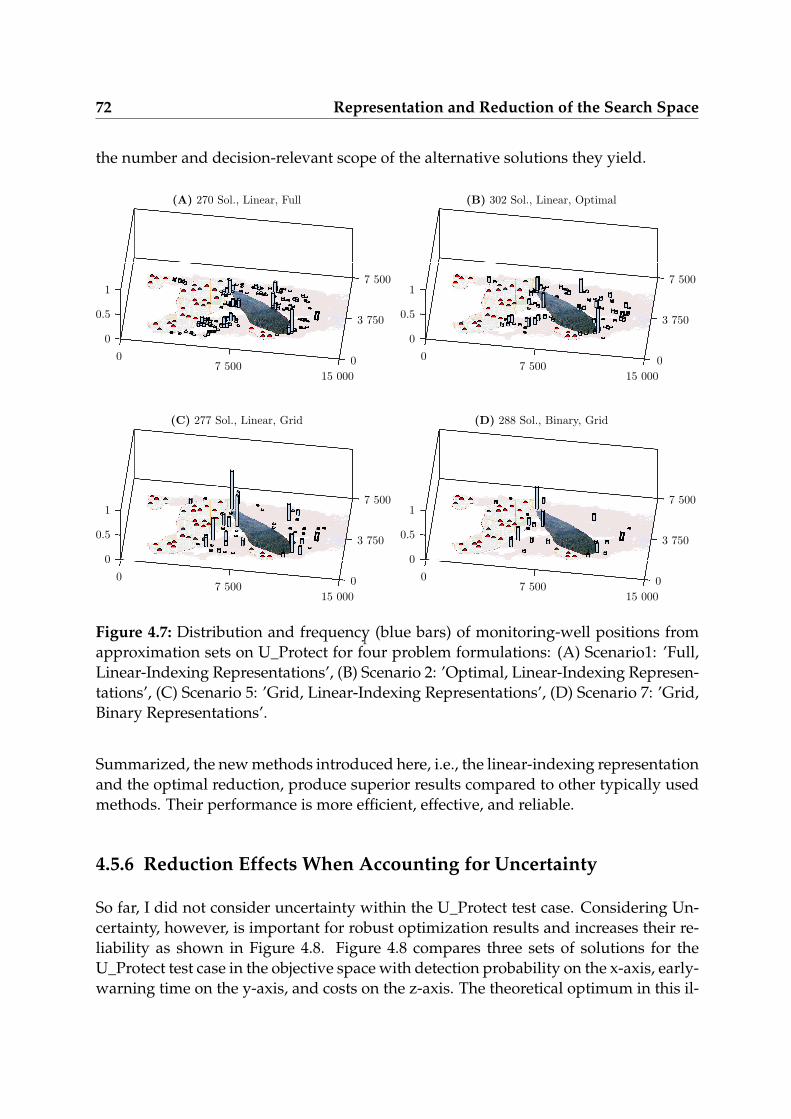
72 Representation and Reduction of the Search Space

the number and decision-relevant scope of the alternative solutions they yield.

(B) 302 Sol., Linear, Optimal

0

0.5

1

07 500

15 000

0

3 750

7 500

(A) 270 Sol., Linear, Full

0

0.5

1

07 500

15 000

0

3 750

7 500

(C) 277 Sol., Linear, Grid

0

0.5

1

07 500

15 000

0

3 750

7 500

(D) 288 Sol., Binary, Grid

0

0.5

1

07 500

15 000

0

3 750

7 500

1Figure 4.7: Distribution and frequency (blue bars) of monitoring-well positions fromapproximation sets on U_Protect for four problem formulations: (A) Scenario1: ’Full,Linear-Indexing Representations’, (B) Scenario 2: ’Optimal, Linear-Indexing Represen-tations’, (C) Scenario 5: ’Grid, Linear-Indexing Representations’, (D) Scenario 7: ’Grid,Binary Representations’.

Summarized, the new methods introduced here, i.e., the linear-indexing representationand the optimal reduction, produce superior results compared to other typically usedmethods. Their performance is more efficient, effective, and reliable.

4.5.6 Reduction Effects When Accounting for Uncertainty

So far, I did not consider uncertainty within the U_Protect test case. Considering Un-certainty, however, is important for robust optimization results and increases their re-liability as shown in Figure 4.8. Figure 4.8 compares three sets of solutions for theU_Protect test case in the objective space with detection probability on the x-axis, early-warning time on the y-axis, and costs on the z-axis. The theoretical optimum in this il-

4.5 Results and Discussion 73

lustration is the backside lower-left corner. The orange set is a Pareto-front approxima-tion for a single scenario, i.e., for U_Protect without considering uncertainty. The blueset is a Pareto-front approximation for multiple scenarios (around 300), i.e., with con-sidering uncertainty in U_Protect. The red set illustrates the performance of the orangesolutions (without uncertainty) on the U_Protect test case with uncertainty considered.For a better understanding of the three sets, all candidate solutions are projected on thetwo-dimensional planes. Figure 4.8 clearly shows that the optimization problem be-comes more challenging when considering uncertainty (blue): the candidate solutionscannot reach the same quality level as the solutions without considering uncertainty(orange). It also illustrates the quality loss in performance when ignoring uncertainty(red vs. blue). Consequentially, uncertainty consideration helps prevent frustrationdue to high but unfulfilled expectations (in Figure 4.8: expected performance (orange)vs. effective performance (red)). Although the blue set totally outperforms the redset, the blue set is located in a critical objective-space range where any deviation fromthe real Pareto front should be as small as possible. The actual goal attainment nei-ther exceeds 50% in early-warning time, nor in detection probability. That is, the goalattainment is low and the potential loss of, e.g., 1% detection probability is relativelylarger compared to the case without considering uncertainty (orange). Concluding,with uncertainty consideration, an effective optimization is particularly desirable.

We already saw that the linear-indexing representation of the search space is preferredover the binary representation and, with the optimal reduction method, the optimiza-tion provides superior results. With uncertainty consideration, however, the base EDOset becomes more challenging for two reasons:

1. As I use the arithmetic mean to aggregate over all scenarios (cf. Section 3.4), thefinal EDO set enlarges compared with the single-scenario EDO set (in our case:219,122 vs. 436,986 EDOs), because the possibly contaminated area increases withthe number of possible flow paths for the possible contaminations.

2. Due to the averaging effect, the aggregated objective values of the single EDOsbecome similar (the EDO set becomes indifferent) and less EDOs are clearly dom-inated, hence can be removed.

While the linear-indexing representation is not affected by the more complex ’uncer-tainty’ EDO set, the optimal reduction is presumed to be less effective and less ef-ficient (less EDOs to remove, more EDOs to compare). A measure to increase bothefficiency and effectiveness of the reduction algorithm is to use the boosted optimalreduction method introduced in Section 4.3. The boosted version homogenizes the ob-jective space of the EDO set and more EDOs can be removed. Here, we use the round-function as homogenizer. Differently to the pure optimal reduction method, with theimplemented homogenization, it cannot be guaranteed anymore that the EDO set con-tains all Pareto-optimal solutions. However, compared to the pure optimal reductionmethod, the boosted one totally outperformed (cf. Table 4.7): it is much faster and

74 Representation and Reduction of the Search Space

1

0.5

0De

tectio

n Proba

bility

[-]

1 0.5 0Benefit of EWT [-]

0

0.5

1

Costs[$]

1

Figure 4.8: Pareto-approximations sets in the objective space. Orange spheres: approx-imation set without considering uncertainty. Blue spheres: approximation set withconsidering uncertainty. Red spheres: performance of the orange solutions (withoutuncertainty) when confronted with uncertainty. Dots: projection of the sets on therespective two-dimensional planes.

more effective. The question is, whether the missing guarantee of optimality has asignificant drawback on the optimization.

Therefore, Figure 4.9 shows again the hypervolume dynamics as a function of NFEfor the three alternative problem formulations with uncertainty consideration (cf. Ta-ble 4.3). All are based on the linear-indexing representation. The ’Full’ problem for-mulation (Scenario 8) uses the base EDO set, the ’Optimal’ formulation (Scenario 9) isbased on the optimal-reduced EDO set, and the ’Optimal + Round’ EDO set (Scenario

Table 4.7: Efficiency and Effectiveness of the Pure and Boosted Optimal ReductionMethod

Method Wall-Clock Time Total Reduction Reduction Rate

Pure Optimal ∼ 10, 800 s 367,784 ∼ 84%Boosted Optimal ∼ 150 s 436,185 ∼ 99.8%

4.5 Results and Discussion 75

10) is based on the optimal reduced EDO set by the round-function boosted optimal-reduction method (cf. Section 4.3). Both reduced problem formulations are more effi-cient compared with the ’Full’ problem formulation. The latter needs around 107 NFEto reach the same hypervolume as the ’Optimal’ formulation after 6 × 105 NFE. After5 × 107 NFE, it reaches the same hypervolume as the ’Optimal + Round’ formulationafter 5 × 105 NFE. Obviously, the size of the different EDO sets is the main player forthe optimization performance. Although the ’Optimal + Round’ formulation cannotguarantee to provide all Pareto-optimal solutions, it clearly outperformed the othertwo formulations.

Hypervolume

NFE

0.5

0.75

1

103

Full

Optimal

Optimal + Round

104 105 106 107 108

1

Figure 4.9: Runtime dynamics: Hypervolume over function evaluations (NFE) forthree problem formulations (Scenarios 8-10) that differ in the used EDO set. All prob-lem formulations are based on the linear-indexing representation. As in Figure 4.4,the shaded areas represent variations in hypervolume and are bounded by the 10%and 90% percentiles. The solid lines represent the median for the respective problemformulation. Due to the large number of function evaluation for the ’Full’ problem for-mulation (please observe the logarithmic scale), data are available every 50,000 NFE.

Summarized, the ’Optimal + Round’ formulation showed the best optimization perfor-mance and the EDO-set reduction is highly efficient and effective. Especially for shortoptimization wall-clock times, the rigorous but slow optimal reduction method is notadvisable. The optimal reduction method works best for (1) heterogeneous EDO sets,i.e., with EDOs that can clearly be distinguished in their objective values, and (2) forhomogeneous EDO sets, i.e., with EDOs that have the same objective values. Then, theoptimal reduction would provide small EDO sets that are ideal for producing superiorresults with MOEAs. When considering uncertainty, however, the aggregation effectsmake the EDO set indifferent, i.e., with EDOs that are similar to each other, and the

76 Representation and Reduction of the Search Space

reduction is less effective. In this case, the reduction can be supported by a homoge-nization method that equalizes similar EDOs.

4.6 Summary and Conclusions

This chapter approaches challenges that emerge when addressing discrete multi-objective optimization problems with large potentially severe combinatorial scalingin their decision spaces. Specifically, I (1) developed an efficient and reliable search-space representation, the linear-indexing representation, that can handle large deci-sion spaces, and (2) I contribute a search space reduction method, the optimal reduc-tion, that provides speed search while ensuring the attained multi-objective trade-offsare improved high-quality approximations to the true Pareto-optimal solutions. Asbenchmark, I use the U_Protect test case together with the general optimization prob-lem (formulated in Section 3.2) with three objectives: (1) detection probability (to bemaximized), (2) early-warning time (to be maximized), and (3) costs (to be minimized).

I compare the linear-indexing representation with the common binary representation.My analysis shows that:

1. Linear-indexing representation enables reliable and efficient optimization runsthat clearly outperform the binary representation over time.

2. Unlike binary representation, the linear-indexing representation can handle largeproblems.

I also compare our optimal search space reduction method with optimization-basedand grid-based reduction methods. The grid-based reduction methods can be appliedto continuous and discrete problems and are independent of the objective functions,the optimal and optimization-based reduction methods are limited to discrete prob-lems and monotonous objective functions. In the context of the U_Protect test case, Ishow that:

1. Optimal reduction strategies produce the best results but need an additional al-gorithm.

2. The grid-based reduction is highly effective but a brute-force approach with thepotential of losing candidate Pareto-optimal monitoring alternatives.

3. Optimal reduction gets performance problems for highly indifferent decisionspaces, but can be boosted with methods that homogenize them.

The overarching conclusion is that, for discrete problems, linear-indexing represen-tation is the key for a reliable and efficient optimization performance. Also, when-ever feasible, my proposed optimal reduction helps to improve quality and endpoint

4.6 Summary and Conclusions 77

value of multi-objective analyses for the design of groundwater monitoring systemsfor source water protection.

These insights can be transferred to a broad class of optimization problems. The fol-lowing four conditions must be fulfilled to apply linear-indexing representation andoptimal reduction:

1. The search space must be finite, as part of a discrete and finite optimization prob-lem (for representation and reduction).

2. The problem must be a combinatorial problem with a search space that can berepresented by a set of single decision elements (for representation and reduc-tion).

3. The optimization problem must be multi-objective (for reduction).

4. The objective functions must be monotonic (for reduction).

The results enable the feasibility of multi-objective optimization might be possible onstandard desktop computers in operationally valid runtimes.

Chapter 5

Problems and Solutions: Robust andReliable Early-Warning Monitoring inPractice

Parts of this chapter have been published in the Journal TRANSPORT IN POROUS ME-DIA under the title Optimization for Early-Warning Monitoring Networks in Well Catch-

ments Should Be Multi-objective, Risk-Prioritized and Robust Against Uncertainty [19] andin the Journal WATER RESOURCES RESEARCH under the title Reconnecting Stochastic

Methods with Hydrogeological Applications: A Utilitarian Uncertainty Analysis and Risk As-

sessment Approach for the Design of Optimal Monitoring Networks Bode et al. (2018b) [15].I am reusing parts of the text and figures from these publications by the kind permis-sions of the publishers Springer and American Geophysical Union.

In Chapter 3, I introduced the optimization problem and showed that good trade-offsolutions can be found. In Chapter 4, I specified the problem formulation with a focuson search-space reduction and representation. I showed that the linear-indexing rep-resentation is significantly more reliable and efficient compared to the classical binaryrepresentation. I also introduced possible reduction methods for the search space thatcan lead to better optimization results and to an easier handling of a large data volume.Although I could increase efficiency and effectiveness of the optimization with themethods introduced in Chapter 4, in practice, there are more fundamental challengesthat may prohibit a straightforward application of such optimization approaches.

These challenges already occur in the preparation phase before the optimization. Manyacademic methods are fundamental and general, but not yet optimized for practi-cal applications. This holds, in particular, for advanced methods in stochastic hy-dro(geo)logy, uncertainty quantification, and risk analysis. Many academic risk es-timation methods emphasize rigorously quantitative results [e.g., 28, 159], which re-quires input data that are rarely available in practice. For water suppliers, however, itis especially difficult to collect the required data. For instance, the effort is very highto explore the catchment for possible contamination sources and to collect all requiredcharacteristics of these sources, and there are difficulties in evaluating their respectiverisk. Additional difficulties are caused by limitations in time and computing power fortransport simulations, especially when uncertainty in hydro(geo)logy and/or locationuncertainty of possible contamination sources is considered.

5.1 Simplifying Breakthrough Curve Approximation 79

In this chapter, I present methods and strategies for tackling the following specificchallenges:

• Water suppliers usually do not have access to high-performance computingclusters, while transport simulations and uncertainty quantification are oftencomputationally demanding. Thus, water suppliers need strategies that arefrugal enough to perform such tasks on standard desktop computers (Sec-tions 5.1 and 5.3).

• Especially in urban areas, too many possible contamination sources could existto be screened effectively. Therefore, water suppliers need to distinguish relevantfrom irrelevant sources to reduce the number of considered sources (Section 5.2).Still, the number of relevant sources might be large, hence they also need effec-tive methods to downsize the number of relevant sources during the transportsimulation (Section 5.5).

• Possible contamination sources must be treated differently according to the riskthey pose for the supply wells. However, it is difficult or even impossible to de-termine their risk quantitatively. That is, water suppliers need a non-quantitativepossibility to prioritize their inventory of possible contamination sources duringthe optimization (Section 5.4).

• It is very likely that many possible contamination sources exist that are unknown.A coordinated monitoring of these sources is not possible, but in fact, unknownsources are a big issue. Hence, water suppliers need a strategy to account for theneed to monitor unknown sources (Section 5.6).

In the following sections, I will briefly explain the specific problems and introduceapproaches how I tackle them. For clarification and/or conformation of the used ap-proaches, I will present and discuss supporting results, if it is helpful. At the end ofthis chapter, I will summarize the main conclusions in Section 5.7.

5.1 Simplifying Breakthrough Curve Approximation

As mentioned in Section 2.3, I use the PTRW method in all transport simulations to ap-proximate the spatial and temporal concentration distributions of contaminants. Thestraightforward way to simulate the related breakthrough curves in a control volume(CV) is to track the number and residence time of the particles that pass the respectiveCV. Knowing the volume V

[L3]

of the ith CV, and the mass mp [M] of each particle j,one can easily approximate the breakthrough curve by counting the particles over timeat volume i:

ci (t) ≈1

ne,iVi

np

∑j=1

δijmp,j , (5.1)

80Problems and Solutions: Robust and Reliable Early-Warning Monitoring in

Practice

with the effective porosity ne in Vi, the number of all particles np, and the Kroneckerdelta δij that indicates whether particle j occupied volume i or not (1 or 0). However,this counting technique leads to discontinuous breakthrough curves. For continuousbreakthrough curves, more advanced methods must be applied, e.g., kernel densityestimation [129].

For PTRW, the approximation error of breakthrough curves decreases proportionallyto the square root of the number of particles in each CV [e.g., 84]. That is, for largemodel domains, millions of particles are needed, and this leads to computationally de-manding simulation runs. A common technique for reducing computational costs is toapproximate the temporal moments of breakthrough curves, instead of approximatingthe entire curve [e.g., 77, 104]. Then, the breakthrough curve can be reconstructed withparametric shapes from these moments. The advantage is that temporal moments aremore robust against low particle numbers so that the total number of particles can bereduced dramatically. A requirement of this technique is that an analytical parametricdistribution function is available that is defined by the temporal moments and meetsthe general behavior of the real curves (i.e., the shape).

In Section 2.2, I already introduced the inverse Gaussian distribution (IG). The IG is theanalytical solution for breakthrough curves of an instantaneous contamination releasein uniform and parallel flow with uniform dispersion coefficient. The scaling factormIG

0 [MT/L3] of the IG is the zeroth moment of the breakthrough curve, i.e., it matchesthe time integral over the entire curve. It can be approximated as:

mIG0,i ≈

1ne,iVi

np

∑j=1

δijmp,j∆tj , (5.2)

with the residence time ∆tj [T] of particle j in CV Vi. Then, the breakthrough curve canbe reconstructed as

ci (t) ≈ mIG0,i IG . (5.3)

For continuous mass release, the breakthrough curve is the temporal convolution ofEquation 5.3:

Ci (t) ≈∫ t

0mIG

0,i IGdτ , (5.4)

with the contaminant release time τ. Equation 5.4 can be rearranged when substitutingthe mass mp,j in Equation 5.2 by the constant value mp,j =

∫ mp,jτ dτ:

MIGC0,i ≈ 1

ne,iVi

np

∑j=1

δijmp,j∆tj . (5.5)

Then, continuous breakthrough curves can be expressed using the cdf of the IG (cf.Equation 2.13):

Ci (t) ≈ MIGC0,i

∫ t

0IGdτ = MIGC

0,i · IGC (τm) . (5.6)

5.1 Simplifying Breakthrough Curve Approximation 81

In order to show that the reconstructed breakthrough curves need significantly fewerparticles compared to the straightforward density estimation via particle counting, Iuse a quasi-three-dimensional uniform velocity field (15m × 10m × 10m), instanta-neously release particles at (x = 5, y = 5), and measure the concentration over timeat (x = 15, y = 5). The time discretization is 10s and the dimension of the CV is(0.7m × 0.7m × 10m). Transport-relevant parameters can be found in Table 5.1. I alsocompare the reconstructed curves with an analytical solution for this problem to bettershow how the reconstructed curves are affected by particle reduction. Therefore, I usethe depth-integrated analytical solution of the concentration distribution over time atlocation (x, y) that is given by Equation 5.7 [e.g., 8]:

c (t, x, y) =m

B

14πt

√DLDT

· exp

((−x + vt)2

4DLt− y2

4DTt

), (5.7)

with the released mass m, aquifer depth B, time t, velocity v, and longitudinal andtransverse dispersion coefficients DL and DT.

Figure 5.1 shows four different approximations of the breakthrough curve with dif-ferent numbers of particles. It clearly indicates that the moment-based breakthroughcurves (green line) are less affected by small particle numbers than the particle-counting-based approximation. The deviations between the moment-based and theanalytical curves are small for each case, while the particle-counting-based curve isnot reliable with 10000 particles or less.

Although the scaled IG does not generally hold for realistic cases (e.g., with non-uniform flow), I chose this reconstruction method in general over the particle-countingmethod for two reasons:

1. Computational power is limited in practice, hence practitioners need robust andefficient methods.

2. Many groundwater models are built with standard software suites like ModFlowand use relatively simple zonations to represent heterogeneities. Within the zona-tions the assumption of uniform flow is acceptable.

Table 5.1: Transport-relevant parameters.

Initial massm [kg]

Velocityv [m/s]

MoleculardiffusioncoefficientDm

[m2/s

]

Longitudinaldispersivityαℓ [m]

Transversedispersivityαt [m]

0.01 0.01 1 × 10−9 1 0.1

82Problems and Solutions: Robust and Reliable Early-Warning Monitoring in

Practice

Time in seconds

0 1000 2000 3000

Concentrationin

kg

m3

0

1

2

350000 Particles×10−5

Time in seconds

0 1000 2000 3000

Concentrationin

kg

m3

0

1

2

310000 Particles×10−5

Time in seconds

0 1000 2000 3000

Concentrationin

kg

m3

0

1

2

31000 Particles×10−5

Time in seconds

0 1000 2000 3000

Concentrationin

kg

m3

0

1

2

3500 Particles×10−5

Hist.

Anal.

Mome.

1

Figure 5.1: Comparison of particle-counting-based breakthrough curves via histogram(gray) with reconstructed curves (green) and the analytical solution (red).

5.2 Defining the Catchment

In many countries, groundwater protection zones restrict activities and storage of pol-lutants that are hazardous to water, but they cannot eliminate all water-hazardous pol-lutants, such that an inventory of possible groundwater contamination sources remains(see discussion in Chapter 1). These possible sources need to be monitored effectivelyto protect the water supply wells from contaminations if they fall into by the wellcatchment. Protection zones and actual well catchment often differ starkly in extentand location. Although both are based on the hydrogeological conditions [e.g., 46], thedefinition of protection zones is often practically and/or politically constrained. An al-

5.3 Uncertainty and Robust Optimization 83

ready existing highway, for example, would not be rerouted if it goes straight througha currently defined catchment.

To provide clarity, as first and most important step, I propose to approximate the realwell catchment (using backward transport simulation [122]) for four reasons:

1. The catchment could be just partly covered by the protection zone. Contamina-tion sources outside the protection zone, but inside the catchment, still put theproduction wells and the produced water at risk.

2. Parts of the protection zone might not coincide with the actual catchment. Then,there may be contamination sources within the protection zone that do not af-fect the production wells, because they are not within the catchment. They areirrelevant for the water supplier.

3. Using backward transport simulation, one can estimate how much contaminantmust be released at a certain location to still affect the production wells. Possiblesources that cannot release the required mass of a contaminant are irrelevant forthe water supplier, even if they fall into the catchment.

4. Using backward transport simulation, one can estimate the travel times fromeach location towards the production wells. Possible contamination sources thatneed longer than a certain time threshold to affect the production wells might beagain irrelevant for the water supplier.

In summary, defining the well catchment, critical masses and travel times can guidewater suppliers in their search for relevant possible contamination sources. Focusingonly on the relevant sources identified in a reverse transport simulation reduces thecomputational demand of the subsequent forward transport simulations from all pos-sible contamination sources to the supply wells. From the economic point of view,identifying irrelevant sources prevents the water supplier from installing monitoringwells that are useless.

To implement backward simulation, I invert the velocity field and solve a reverse trans-port problem (cf. Section 2.3) that starts at the production well. The resulting backwardplume identifies the transport-relevant catchment of the well that needs to be moni-tored. Figure 5.7 in Section 5.6 exemplary shows relevant (green, yellow, and red dots)and irrelevant (gray dots) possible contamination sources as identified by the back-ward transport calculation. The optimized monitoring network (black crosses) onlyfocuses on the relevant sources.

5.3 Uncertainty and Robust Optimization

When looking at the relatively thin predicted plumes occurring in Z_Based in Fig-ure 5.3, it is apparent that the "real-life" performance of optimized early-warning mon-

84Problems and Solutions: Robust and Reliable Early-Warning Monitoring in

Practice

itoring networks (compared to the performance predicted during the optimization) ishighly sensitive to predictive uncertainty. Therefore, in Section 3.4, I suggested to in-clude a corresponding representation of uncertainty during the optimization in orderto achieve robustness. I call a monitoring network robust against a given uncertaintyif its performance does not fall below expectation under the corresponding range ofpossibilities. In the following, I will discuss representations of uncertainty, effects ofuncertainty, and the benefits of robust optimization.

Representation of Uncertainty

Geostatistically-based Monte-Carlo (MC) simulation is the standard academic ap-proach to account for statistical uncertainty of aquifer parameters in groundwatermodels [e.g., 59, 65, 138]. However, in practice, MC simulations are impractical forfour reasons. First, they are computationally too expensive to apply to large-scale orcomplex models typically needed for practical problems. Second, the underlying prob-ability distributions of the uncertain parameters are not easy to define such that theywould represent a realistic level of uncertainty. Third, numerical models used by watersuppliers are usually built with standard software like ModFlow [74] or FeFlow [160]that lack a convenient interface for running MC simulations. Fourth, it is much easierto operate that type of software with zonation-based parametrizations or with pilotpoints [e.g., 132, 42] than with geostatistical random fields [e.g., 40, 88].

Despite these limitations, hydrogeologic uncertainty must be considered in the opti-mization to propose reliable network designs. Discussions with water suppliers ledme to represent uncertainty by using well-selected scenarios instead of formal MCanalyses. These scenarios have to satisfy two requirements:

1. They have to represent the dominant uncertainties that most influence the loca-tion and concentration of possible contaminant plumes.

2. The ensemble of scenarios should be chosen such that they cover the entire vir-tual contaminated area between the two enveloping plumes of this ensemble (anexample of well-selected scenarios is shown in Figure 5.2 for uncertainty in am-bient flow direction).

Further criteria for the quality of scenarios are discussed, e.g., by Kosow andGaßner (2008) [97].

Intense discussions with water providers showed that, for most of the well catchments,the ambient flow direction is the most influential factor. It is controlled by seasonalchanges in groundwater recharge and by the pumping rate of the production wells.Catchments for other supply wells were highly influenced by the stages of nearby

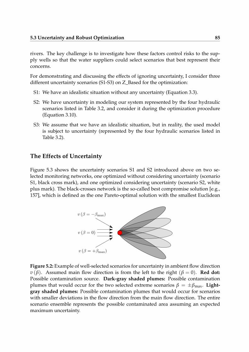
5.3 Uncertainty and Robust Optimization 85

rivers. The key challenge is to investigate how these factors control risks to the sup-ply wells so that the water suppliers could select scenarios that best represent theirconcerns.

For demonstrating and discussing the effects of ignoring uncertainty, I consider threedifferent uncertainty scenarios (S1-S3) on Z_Based for the optimization:

S1: We have an idealistic situation without any uncertainty (Equation 3.3).

S2: We have uncertainty in modeling our system represented by the four hydraulicscenarios listed in Table 3.2, and consider it during the optimization procedure(Equation 3.10).

S3: We assume that we have an idealistic situation, but in reality, the used modelis subject to uncertainty (represented by the four hydraulic scenarios listed inTable 3.2).

The Effects of Uncertainty

Figure 5.3 shows the uncertainty scenarios S1 and S2 introduced above on two se-lected monitoring networks, one optimized without considering uncertainty (scenarioS1, black cross mark), and one optimized considering uncertainty (scenario S2, whiteplus mark). The black-crosses network is the so-called best compromise solution [e.g.,157], which is defined as the one Pareto-optimal solution with the smallest Euclidean

Figure 5.2: Example of well-selected scenarios for uncertainty in ambient flow directionv (β). Assumed main flow direction is from the left to the right (β = 0). Red dot:

Possible contamination source. Dark-gray shaded plumes: Possible contaminationplumes that would occur for the two selected extreme scenarios β = ±βmax. Light-

gray shaded plumes: Possible contamination plumes that would occur for scenarioswith smaller deviations in the flow direction from the main flow direction. The entirescenario ensemble represents the possible contaminated area assuming an expectedmaximum uncertainty.

86Problems and Solutions: Robust and Reliable Early-Warning Monitoring in

Practice

0 m 7 500 m 15 000 m

0 m

3 500 m

7 000 m

1

Figure 5.3: Two selected optimized monitoring networks from the basic multi-objectiveoptimization without uncertainty (black cross mark) and with uncertainty (white plusmark) (see Equations 3.3 and 3.10 in Sections 3.2 and 3.4). Entire blue area: well catch-ment from all hydraulic scenarios; Dark blue area: well catchment from hydraulic sce-nario 1. Black rectangle: position of the well gallery; Red points: possible contam-ination sources. Gray dot clouds: visualization of the simulated plumes from eachpossible contamination source for all hydraulic scenarios; Dark gray dot clouds: simu-lated plumes for hydraulic scenario 1. The different hydraulic scenarios can be foundin Table 3.2

.

5.3 Uncertainty and Robust Optimization 87

distance to the idealistic unattainable optimum in normalized axes (cf. Chapter 3).Through optimized positioning of only eight monitoring wells, it attains a detectionprobability of 91% and an early-warning utility of 0.73. This relatively high perfor-mance at relatively low costs can be achieved by two strategies:

1. monitoring the well catchment at positions where several predicted contaminantplumes coincide and neglecting possible contamination sources that have clearlyseparated plumes;

2. by avoiding to attain early warning functionality by covering the most remotesources.

The network considering uncertainty has a similar performance in detection proba-bility and early-warning time, but for reaching these goal attainments it needs elevenmonitoring wells (i.e., three additional ones). It follows the same strategies as the net-work discussed above, but the density of each monitoring-well group increased. Therelatively thin plumes only overlap in the close vicinity of the production wells. Thatis, demanding the same number of monitoring wells when considering different hy-draulic scenarios would push the monitoring network towards the production welland early-warning time would suffer.

The Benefit of Robust Optimization

Figure 5.4 shows the obtained fronts for the three uncertainty scenarios S1-S3. A suit-able measure of robustness is the difference between the optimized predicted perfor-mance and the particular performance obtained after actual installation. For bettercomparison within a single figure, it shows only projections onto the cost/time plane.Scenario S1 (black) performs the best, compared to the other fronts. However, in prac-tice, a scenario without uncertainty does not exist. Considering uncertainty (scenarioS2), the results (red) are more modest in their claims of performance during the opti-mization compared to those without uncertainty (black). The results are less optimisticbecause it is harder to guarantee a reliable and early detection of contaminant plumeswhen admitting that one does not know their exact locations and mutual overlaps.Ignoring uncertainty (scenario S3) leads to differences between the expected perfor-mance (black) and the actual performance in simulated virtual reality (green), i.e., eval-uated for and averaged over all considered hydro(geo)logic scenarios. In theory, themost expensive solution (from the black front) has a close-to-perfect benefit in early-warning time. Compared to that, the same solution performs poorly in virtual reality(green).

Compared to the green front, one could either find monitoring networks with the sameperformance in early-warning time but with fewer costs, or monitoring networks with

88Problems and Solutions: Robust and Reliable Early-Warning Monitoring in

Practice

fwarn

0 0.5 1

fcosts

0

0.5

1

Scen. 1

Scen. 2

Scen. 3

1

Figure 5.4: Projection of Pareto fronts for three multi-objective optimization scenarios.Scenario 1: Black front from an optimization that does not consider uncertainty. Sce-nario 2: Red front obtained when optimizing the performance on average over fourhydraulic scenarios. Scenario 3: Green front illustrates the performance of the non-robust optimization results on average over the four hydraulic scenarios.

a much better performance with identical costs. Obviously, the black solutions are onlyoptimal for one hydraulic scenario, but not for the considered uncertainties.

The difference in early-warning time between the black front and the red front at givencost values can be interpreted as the costs of having (and considering) uncertainty.The difference between the black front and the green front at given cost values canbe interpreted as costs of not considering uncertainty, and these costs are larger thanthe costs of considering uncertainty. Without any surprise, all scenarios agree that onecannot expect any performance at the limit of no costs.

As a conclusion, considering uncertainty in the optimization is in fact required, becauseotherwise, one will obtain overly optimistic model-based results that do not performas desired when installed in reality. The hydraulic scenario analysis performed here isvery crude and serves mainly for illustration. In practice, it would be advisable to alsoaccount for the other sources of uncertainty mentioned in Section 2.4 and to work witha much larger number than the four hydraulic scenarios from Table 3.2, following therules of well-selected scenarios discussed above. Using well-selected scenarios, onecan adopt more efficient approaches that explicitly consider high-risk scenarios. Thiscan build on the years or even decades of experience of water suppliers to propose aset of representative scenarios.

5.4 Risk Prioritization of Possible Contamination Sources 89

5.4 Risk Prioritization of Possible Contamination Sources

The optimization problems formulated in Chapter 3 and in the previous sections ofChapter 5 do not yet prioritize according to the severity of possible contaminationsources. A possible contamination source can be more or less severe depending onthe type of the hazardous activity, stored or handled contaminants and contaminantmasses, compliance with applying regulations and so forth. A common approach toprioritize possible contamination sources is to assign a (statistically motivated) weightto each source that reflects factors like the frequency of accidents, the stored contam-inant mass, mobility, and toxicity. Provided that all required data are available tocalculate these weights through quantitative and probabilistic risk estimations [e.g.,50, 52, 60], this approach would be statistically rigorous. Unfortunately, it is often im-practical, or sometimes even impossible to get all relevant data concerning the possiblecontamination sources (e.g., the probability of failure of a nuclear power plant). Henceit becomes impossible to conduct the probabilistic analyses required to define quanti-tative weights.

Therefore, following concepts of qualitative risk assessment and to provide a practi-cal possible contamination-source prioritization that also supports the individual con-cerns of water suppliers, I categorize all possible contamination sources into the classessevere, medium and almost tolerable [e.g., 26, 78]. This categorization can be visualizedthrough the color scheme of traffic lights, i.e., as red, yellow and green. It expresses theprioritization preferences for monitoring in the sense that "red" possible contaminationsources should be monitored with first priority, "yellow" ones with secondary priority,and "green" ones with the smallest priority.

In order to accommodate this categorization in the optimization problem, I introduceseparate objective functions for the detection probability and for the early-warningtime of each risk category. Because individual monitoring wells can cover possiblecontamination sources from several risk categories, the cost function cannot be sepa-rated. Thus, the original problem with three objectives

dopt = arg mind∈D

( fdetect, fwarn, fcost) (5.8)

obtains a total of seven objectives:

dopt = arg mind∈D

[f(red)det , f

(red)warn , f

(yellow)det , f

(yellow)warn , f

(green)det , f

(green)warn , fcost

]. (5.9)

Although the optimization became more complex, the benefit of this approach is thatwater suppliers can prioritize the possible contamination sources following their ownindividual assessment, expert opinion, or public concerns. This is possible without theneed for a difficult and costly acquisition of data to calculate quantitative risk weights.

90Problems and Solutions: Robust and Reliable Early-Warning Monitoring in

Practice

For demonstrating and discussing the qualitative risk prioritization, I present opti-mization results of the optimization problem according to a robust formulation ofEquation 5.9, i.e., working with a risk categorization and uncertainty. In this opti-mization, I categorize the inventory of possible contamination sources of Z_Based intosevere, medium and almost tolerable sources, and compare the results to those ob-tained without risk categorization according to Equation 3.10 (see Section 3.4).

In Figure 5.5, I compare a selected Pareto-optimal monitoring network from the risk-prioritized formulation (black cross marks) with a selected one obtained from Sec-tion 5.3, i.e., without risk prioritization. The prioritized solution was selected toachieve a 100% detection probability and a large early-warning time utility (here: 86%)for all severe possible contamination sources (red ones) while maintaining the numberof monitoring wells at eleven, i.e., using the same number as the non-prioritized solu-tion. This results in a reduced detection probability and early-warning utility acrossthe remaining risk inventory. The key performance data of both networks can be foundin Table 5.2. By comparison of these two networks, one can see that two additional se-vere possible contamination sources (red) are now monitored (one at [4km, 1.5km] indomain coordinates and one at [7km, 3km]). One monitoring well roughly at [7km,4km] has been removed, because it mainly served to monitor medium and almost tol-erable (yellow, green) possible contamination sources. Other significant changes ap-pear around [11km, 4.5km], where a group of three monitoring wells was replaced by

0 m 7 500 m 15 000 m

0 m

3 500 m

7 000 m

1

Figure 5.5: Comparison of a risk-prioritized solution from the robust multi-objectiveoptimization with a solution without risk categorization. Black cross marks: prior-itized monitoring network; White plus marks: network without prioritization; Red,yellow, green dots: prioritized possible contamination sources; All other symbols andcolors: same as in Figure 5.3.

5.5 Areas with Many Possible Contamination Sources 91

two monitoring wells that coincide better with the possible plume paths of only severepossible contamination sources (red).

There are several strategies available for decision makers to screen through the list ofPareto-optimal results. One option is to screen through the possible compromises be-tween overall coverage and prioritized coverage at fixed costs. A second option is tostart with perfect coverage of severe sources, and then to investigate the additionalcosts and willingness to pay for additional coverage of medium and almost tolerablesources. With this, decision-makers are able to make the necessary compromises be-tween the performance for different risk categories under budgetary constraints in aninformed and transparent manner. They do not have to quantify weights before theoptimization but can see the consequences of their preferences directly at the Pareto-approximation front.

5.5 Areas with Many Possible Contamination Sources

Some possible contamination patterns can be difficult to characterize because they in-clude multiple possible sources distributed in a relatively large area (e.g., cities, land-fills, industrial parks, ...). Practically, it can be too expensive to produce a detailed mapof each source. Furthermore, in many cases, water suppliers do not have the right tocollect all of the information necessary to describe the separate sources. Often, evenif the data could be collected, the computing time and memory requirements to treateach source individually in the transport simulations may be prohibitive. For practicalapplication, this type of source area (area with uncertainty in point-source locations)should be handled using a simpler, representative model.

To accommodate this preference, I introduced the concept of virtual representativesources. Instead of accounting for each possible source in, e.g., an urban area, artificialsources are used, closely spaced along a line at the downstream edge of the source area.The underlying idea is that the plumes emanating from any source within the area willcross this downstream boundary. Furthermore, placing the virtual sources as close as

Table 5.2: Key data of the different monitoring networks illustrated in Figure 5.5

Monitoringnetwork

Riskcategories

Detection Probability[−]

Early-warning timeutility [−]

Non-prioritized All 0.97 0.79Non-prioritized Severe 0.88 0.72Prioritized All 0.80 0.66Prioritized Severe 1 0.86

92Problems and Solutions: Robust and Reliable Early-Warning Monitoring in

Practice

possible to the edges of the source area, with reference to the flow lines, provides aconservative estimate of impact. That is, the virtual contaminants represented by thevirtual contaminant sources will arrive sooner and at higher concentrations than theactual contaminants from the real possible contamination sources within the sourcearea. In most cases, the difference in estimated warning time is small because the sizeof the source area is small relative to the distance of the downstream boundary to theproduction wells. therefore, this simplification provides at least as much protection aswould be provided if every real source was modeled individually; however, it offersthree practical advantages:

1. water suppliers do not need to undertake time-consuming and expensive dataacquisition in urban areas;

2. they can account for possible contamination sources that are uncertain in locationwithin urban areas;

3. the transport simulation requires less computational effort and time to considerthe smaller number of virtual representative sources.

5.6 Unknown Possible Contamination Sources

When designing a monitoring network, the most difficult possible contaminationsources to consider are the (potentially numerous) sources within well catchmentsthat are not even known to exist. Reasons for this include the limited existence ofinformation on land use in the private or industrial sector, restricted access to existinginformation due to data privacy policies, known possible sources with unknown loca-tions (from vague historical records) or unforeseeable hazards that fall under the clas-sical category of black swans [158]. These unknown possible contamination sourcesare especially problematic for water suppliers with production wells in large, denselypopulated areas and in regions with intensive farming. The only way to achieve ro-bustness in the face of unknown sources is to represent the possible existence of themthrough an additional virtual component in the risk model. While it is important toguard against unknown sources, the virtual risk model must be as pragmatic and sim-ple as possible. For example, using a dense grid of virtual sources over the entire wellcatchment would lead to unacceptably high computational costs. I chose to model theunknown risks using a densely spaced set of virtual point sources that surround thewater supply wells (cf. Figure 5.6, the virtual blue possible contamination sources atthe pumping well). In the following, I call this concept line of attack. This risk modelis plausible because any contaminant from (unknown) possible contamination sourceshas to pass the line of attack before affecting the pumping wells. Thus, a resulting mon-itoring network that can monitor the virtual sources on the line of attack is also ableto monitor any remaining risk that is farther away from the pumping wells. For all

5.6 Unknown Possible Contamination Sources 93

unknown spills, the line of attack is a conservative (worst-case) representation in thefollowing aspects (compared to the actual properties of the unknown possible sourcerepresented by this model):

1. the modeled travel time from the line of attack to the well is always shorter;

2. the detectable width of the modeled plumes is always smaller;

3. the contaminant impact on the well is always larger.

The line of attack is located at a distance in travel time coordinates that is defined bythe user. Essentially, this represents the minimum travel time that a user is comfortableallowing themselves to install countermeasures for water quality protection. All resid-ual unknown sources between the line and the pumping wells cannot be controlledwith the resulting monitoring networks. Hence, the choice of travel time to the wellis a compromise between residual-risk coverage and achievable early-warning time.Known possible sources between the line of attack and the pumping wells need to bemonitored with source-targeted wells.

The line of attack approach potentially offers large savings in monitoring costs and indesign optimization. This is because there will be no further advantage in placing anymonitoring wells farther away from the well than the line of attack if only a robustdetection probability is essential and the user-defined minimal early-warning time issufficient. In this case, there is no need to collect data about sources beyond this dis-tance, either. The corresponding monitoring networks usually exhibit a line of defenseformed by monitoring wells just downgradient of the line of attack. However, out-side of the line of attack, there might exist known possible contamination sources toxicenough such that a reliable monitoring in detection probability and early-warning timeis required. Then, additional monitoring wells close to these known possible contami-nation sources are appropriate.

To facilitate the line-of-attack concept, I followed the approach described in Section 5.4and suggest to classify the unknown possible contamination sources into a risk class.However, they are unknown, and hence they cannot be classified into one of the threealready existing risk classes in a meaningful manner. To overcome this problem, I in-troduce an additional risk class (blue) that represents unknown possible contaminationsources in distributed areas and unknown sources placed on a line of attack:

dopt = arg mind∈D

[f(red)det , f

(red)warn , f

(yellow)det , f

(yellow)warn , f

(green)det , f

(green)warn , f

(blue)det , f

(blue)warn , fcost

]

(5.10)With that, the number of objective functions increases again (from seven to nine). But,this further increase in complexity has the benefit of accommodating the subjectiveconcerns and expert judgments of stakeholders, allowing them to alter the weights onthe virtual sources to represent their relative risk tolerance of known and unknownsources.

94Problems and Solutions: Robust and Reliable Early-Warning Monitoring in

Practice

Figure 5.6 shows one selected optimized network, which can be separated in two partswith different tasks: the first part (white pluses) specializes only on good coverage ofthe residual risks (line of defense close to the line of attack), and the second part (whitecrosses) is an augmentation of the line of defense in order to improve the performancein monitoring all the known possible contamination sources. The model for residualrisks is the representation by the line of attack (blue dots) that lies between the wellgallery and the bulk area of the catchment. Here, the line of attack is a line of hypothet-ical point sources placed at a travel time of two years away from the well gallery. Forsimplicity of the analysis, here I drop the classification of the known possible sourcesinto different risk classes.

The performance data for both parts are shown in Table 5.3. The strategy for coveringthe residual risk is the line of defense that directly matches the line of attack. In thesolution shown, this line is composed of 17 monitoring wells. This strategy achieves adetection probability of 81% and claims an early warning utility of 0.68. The detectionprobability number is accurate for all residual risks (behind the line of attack). Theearly warning time, however, is strongly suboptimal, because most residual risks couldbe detected earlier when knowing their location.

The line of defense provides a good coverage for almost all possible residual risksources anywhere in the catchment. Only 19% of the entire catchment area cannot

0 m 7 500 m 15 000 m

0 m

3 500 m

7 000 m

1

Figure 5.6: Comparison of two early-warning networks from the optimization withresidual risks (see Equation 5.10). White plus mark: monitoring network specializedonly on residual risks; White cross mark: augmentation to improve the performancefor the known possible contamination sources; Blue circles: model of residual risk("line of attack"), partly covered by the white cross marks; all other symbols and colors:same as in Figure 5.3.

5.6 Unknown Possible Contamination Sources 95

Table 5.3: Key data of the different monitoring networks illustrated in Figure 5.6

Monitoringnetwork

Sources Detectionprobability

Early-warningutility

Monitoringwells

Only residual Residual 0.81 0.68 17Only residual All known 0.65 0.07 17Augmented Residual 0.81 0.68 26Augmented All known 0.96 0.66 26

be controlled by the line of defense. Hence, it is clear that it should also provide a gooddetection probability for the known possible contamination sources. However, the de-tection probability of the line of defense for all known sources is only 65%. This meansthat 35% of the known sources lay inside the area which is not controlled by the lineof defense, which is more than the 19% predicted during the optimization. This can beexplained by considering the known source inventory as only a small sample out of allpossible source positions (the remaining risk). The early-warning utility for the knownsources is unsatisfactory (0.07). In order to improve this performance, additional mon-itoring wells in the more remote parts of the catchment are required. The cross markshow a selected corresponding augmentation of the current network by 9 monitoringwells. These additional wells increase the detection probability for the known sourcesfrom 65% to 96% and the corresponding early-warning utility from 0.07 to 0.66.

Depending on their risk aversion and risk perception, a decision maker could eitherstart with coverage of residual risks and then buy more early-warning time for knownsources (possibly for the severe ones first), or start with network solutions that offer asatisfactory performance for known possible contamination sources at affordable costs,and then investigate the cost-performance trade-offs for additional coverage of resid-ual risks. The provided information is valuable decision support in situations wheredecision makers are highly risk-averse, or where the residual risks are known to exist atunknown locations. In situations penetrated with deep uncertainty in flow conditions,I expect the residual-risk solution to provide a large degree of robustness.

To show the robustness potential of the line of defense, I compare the performance ofa line of defense (white plus mark in Figure 5.7) to a "regular" monitoring network(black cross mark in Figure 5.7) and show that the line of attack is sufficient to rep-resent unknown possible contamination sources. Therefore, I use the first hydraulicscenario of Z_Based (cf. Table 3.1, here with the longitudinal dispersivity of αℓ = 1mand the transverse dispersivity of αt = 0.1m (cf. Figure 5.7)). I consider 100 scenariosof unknown possible contamination sources. Each of them contains 15 randomly lo-cated unknown and the 15 known possible contamination sources. The ratio of knownand unknown sources is arbitrary and could favor known or unknown sources. Theconsidered domain of all possible locations is restricted to the well catchment.

96Problems and Solutions: Robust and Reliable Early-Warning Monitoring in

Practice

0 m 7 500 m 15 000 m

0 m

3 500 m

7 000 m

1

Figure 5.7: Model domain of the test case. Gray dots: possible contamination sourcesoutside the catchment; Black cross mark: monitoring network with no prioritization;White plus mark: line of defense; all other symbols and colors: same as in Figure 5.3

Figure 5.8 illustrates the performance of both networks for each scenario (blue dots forthe black-crosses network and blue diamonds for the line of defense). They cluster intotwo clouds (illustrated as shaded areas). For both networks, the objective values of theknown possible contamination sources are the same for each considered scenario be-cause they are not affected by the varying unknown sources (cf. the red, yellow andgreen dots/diamonds in Figure 5.8). The line of defense is significantly more robust(against uncertainty in location of possible contamination sources) in terms of detec-tion probability. The variations of the blue diamonds in Figure 5.8 are much smallerthan the variations of the blue dots, and the entire cloud of blue diamonds is close tooptimal detection. The center of the diamonds cloud is approximately at 85% detectionprobability, while the center of the cloud of dots is only near 50% detection probability.There are two reasons for the discrepancy between the expected and actual detectionprobability (100% vs. ∼85%) of the line of defense:

1. The breakthrough curves of a close contamination source might have a short du-ration of visibility at the line of defense so that the probability of missing thecontamination plume due to low sample frequencies increases.

2. The line of defense cannot monitor contamination sources that are within the lineof defense, i.e., between the line of defense and the well gallery.

As expected, the line of defense performs worse in early-warning time compared tothe black-crosses network due to its short distance to the well gallery. However, bud-getary limitations usually make it impossible to install a monitoring network that can

5.7 Summary and Conclusions 97

provide a high detection probability and a high benefit in early-warning time for allunknown possible contamination sources. From this point of view, it is not necessaryto model all possible unknown sources (e.g., using a dense grid of sources over theentire domain) because under cost constraints the optimization algorithm would finda line of defense as Pareto-optimal solution. Relaxing the computationally expensiveapproach of a dense source grid to the line of attack, however, reduces the number ofPareto-optimal solutions. The trade-off between loss in early-warning time and detec-tion probability due to the positioning of the line of defense has to be preselected by thewater supplier. But, especially for well catchments with a difficult inventory of possi-ble contamination sources, i.e., with a high expected number of unknown sources, theline of defense is a strategy worth considering.

In summary, the main benefit of the line of attack is that the corresponding line ofdefense is robust in detection probability against the occurrence of unknown possiblecontamination sources. The main drawback is the loss in early-warning time, becauseof its short distance to the production wells.

5.7 Summary and Conclusions

In this chapter, I presented possible strategies to apply academic concepts in practicesuch that they are frugal enough to run on standard personal computers. For the trans-port simulation, I specifically recommended

• to approximate the temporal moments of the breakthrough curves and then toreconstruct them from those moments, instead of approximating them directly.This way, significantly fewer particles are needed to reach stable breakthroughcurves.

• to determine the catchment of the production wells via backward transport sim-ulation. This step helps to identify and remove possible contamination sourcesthat will be irrelevant in all further analysis steps, because (1) they are outsidethe catchment, (2) they do not contain enough contaminant mass to threaten thewells, (3) the travel time distance of their contaminant is too long.

• to consider uncertainty for robust optimization results, because the actual perfor-mance of optimized early-warning networks is highly susceptible to predictiveuncertainty of contaminant transport towards the well.

Further, I introduced a qualitative risk-prioritization approach that enables water sup-pliers to account for their own (subjective) risk prioritization of each possible contami-nation source instead of difficult (or even impossible) risk-quantification approaches. Ialso presented a strategy to minimize the effort for screening areas with many possiblecontamination sources by representing them with virtual sources. Finally, I introduced

98Problems and Solutions: Robust and Reliable Early-Warning Monitoring in

Practice

Benefit of Early-Warning Time

0% 50% 100%

DetectionProbability

0%

50%

100%

Line of Attack vs. Simulated Scenario Uncertainty

1

Figure 5.8: Trade-off between detection probability and early-warning time for twodifferent monitoring networks. Red and yellow dot (according to the risk class): per-formance of the monitoring network optimized for all known possible contaminationsources (black crosses in Figure 5.7). The green dot is overlain by the red and yellowdot; Red, yellow and green diamonds: performance of the line of defense regarding theknown possible contamination sources; Blue dots: performance of the black-crossesmonitoring network regarding 100 scenarios with 15 randomly located contaminationsources; Blue diamonds: performance of the line of defense confronted with these sce-narios. Black shaded areas: density of the point clouds for a better visibility.

5.7 Summary and Conclusions 99

a risk model that represents unknown possible contamination sources and enable aneffective and robust monitoring.

I find the following conclusions most noteworthy:

• In practice, Monte-Carlo simulations are not feasible to represent uncertainty.Instead, uncertainty can be considered by using representative scenarios. It isimportant to follow the rules of well-selected scenarios and to involve decisionmakers directly and actively in defining the scenarios.

• A prioritization of possible contamination sources and a corresponding augmen-tation of the multi-objective optimization offers options for cost-efficient focus ononly the most severe sources and provides valuable insights into the trade-offs foradditional coverage of medium or almost tolerable sources.

• Early-warning monitoring networks can even be optimized to cover possible con-tamination sources that are unknown in existence or location through an ade-quately chosen residual risk model. The step from quantitative to qualitative riskassessment still requires that possible contamination sources are known in theirlocation and existence. Often, there are unknown possible contamination sourcesin well catchments. In such cases, a useful strategy is to move away from reliablesolutions (in terms of solutions with a quantified probability of success) to robustsolutions (in terms of still serving the purpose sufficiently well and being suf-ficiently reliable even in the face of unknown possible contamination sources).Robustness is typically paid for by a small decrease in classical reliability, or byadditional costs.

Overall, the presented utilitarian approaches serve the goal to adopt computation-ally demanding and data-hungry, complex statistical methods for practical application.Hence, it is one step towards a reconnection of academia and practice.

Chapter 6

An Analytical Approach

This chapter is based on the manuscript An Analytical Approach for Positioning a Single

Monitoring Well to Reliably Detect Point-Source Contaminant Plumes [13]. I am reusingparts of the text and figures from this manuscript.

In the previous chapter, I presented methods and approaches that enable the use ofthe overall optimization approach in practice. Some of these methods dealt with un-certainty in aquifer parameters, or virtual contamination sources that represent, e.g.,possible contamination sources that are uncertain in location. When uncertainty isconsidered, the uncertain parameters become random variables and influence the reli-ability and optimality of possible monitoring-well locations.

Using a proper uncertainty representation (e.g., MC simulation or scenario analysis)for flow and transport simulation and the robust optimization-problem formulationfrom Equation 3.10, an ensemble of varying outcomes can be generated and analyzed.As already shown in Figure 5.4, optimization results for the individual scenarios differfrom the results for the entire ensemble. For instance, without considering locationuncertainty of a contamination plume, a single monitoring well can reliably detect thecontamination everywhere within the plume. With considering location uncertainty ofthe plume, a single monitoring well can reliably detect the contamination only whereall possible plumes overlap. In simulation-based modeling, many more sources ofuncertainty exist.

In this chapter, I specifically investigate the effects of physical mechanisms and param-eter uncertainty on reliable monitoring-well positions. I provide analytical solutionsthat disclose the factors that influence the optimal positioning of monitoring wells witha special emphasis on uncertainty in hydro(geo)logy and spill location. Developing afundamental understanding is crucial for being able to evaluate and understand opti-mal monitoring-network designs. Otherwise, inverse thinking is not possible. In thiscontext, inverse thinking means that decision-makers try to understand the position-ing rules behind an optimization outcome for the sake of validation or learning. Inother words, they might not be able answering the following question:

Why does [some optimization algorithm] suggest these monitoring-well locations

although they do not seem to be optimal to my current understanding?

6.1 Goal, Benefits, and Approach 101

With the fundamental findings of this chapter, optimization results can roughly bepredicted and finally justified.

6.1 Goal, Benefits, and Approach

Goals

The goal of this chapter is to obtain a fundamental understanding of the factors andprocesses that influence the optimal position of a single monitoring well. The moni-toring well should ensure a guaranteed detection of continuous spills that could occurfrom a single possible contamination source. The chance of a guaranteed detection ismainly evaluated by varying flow directions and uncertain spill locations (contaminantplume could by-pass the monitoring well), as well as by varied dilution of the contam-inant due to transverse dispersion (concentration of the contaminant at the monitoringwell could fall below the detection limit). For simplicity, the approach pursued here isdesigned for detecting long-term contaminant sources. Thus, a steady-state approachis employed and monitoring frequency is not considered.

Expected Benefits

The main outcome of this chapter is a fundamental process understanding for findinggood monitoring well positions when conditions are uncertain. Detection monitoringnetworks involving many monitoring points and many contaminant sources are sub-ject to the same underlying processes, albeit with more complexity due to additionalwells and sources. Hence, the results obtained here can be used to better understandand guide formal optimization procedures for monitoring networks and to facilitatethe inverse thinking mentioned above.

Approach

I use an analytical model to determine the optimal monitoring-well locations for asingle contaminant source. A major benefit of employing an analytical approach isthat closed-form expressions for monitoring-well locations can be obtained, directlyexplaining the role of transport parameters. The main interest is on detecting plumesthat emerge from continuous (steady state) point sources of contaminants. Contam-inants are assumed to be conservative, i.e., no sorption or reactions occur. Since thepoint source is continuous, longitudinal dispersion plays only a minor role and can beneglected [e.g., 73].

102 An Analytical Approach

The point source is placed at the origin of the coordinate system, and the two-dimensional steady-state analytical solution of the advection-dispersion equation(ADE) for a depth-averaged infinite aquifer in 2D with constant coefficients (i.e., ho-mogeneous aquifer with uniform thickness and uniform flow) is employed. Here, theGaussian plume is used as solution for the ADE (cf. Equation 2.11). It is mappedto a shifted and rotated coordinate system, such that the contamination source lies atthe origin and the velocity v is aligned with the positive x-axis. We shall call this co-ordinate system the standard space, and denote the coordinates and the concentrationdistribution in the standard space with a tilde: C (x, y).

To compute the concentration at a point (x, y) in physical space, first, it has to be trans-formed to the standard space. We define a transformation T that maps physical coor-dinates into standard coordinates: (x, y) = T (x, y). If the spill location is at (x0, y0) inphysical space and the velocity is rotated by the angle β, then we obtain the followingtransformation T:

(x

y

)=

(cos (β) − sin (β)sin (β) cos (β)

)(x − x0

y − y0

). (6.1)

It follows:C (x, y) = C (T (x, y)) . (6.2)

When considering all parameter values (x0, y0, β) of this transformation to be fixed, theobservable plume concentration C depends only on the spatial coordinates x and y.

Next, a detection limit Cthres is introduced, which depends on the measurement equip-ment accuracy. If the concentration at any point exceeds Cthres, the plume is detectableat that point. Otherwise, it is not. Hence, the isoline C = Cthres from Equation 6.2 out-lines the detectable portion of the plume. In the following, I will only work with thegeometry and outline of the detectable portion, since I am only interested in whetherand where the contaminant spill can be found by detecting its plume. Thus we define:

d (x, y) =

1 if C (x, y) ≥ Cthres

0 otherwise(6.3)

where d (x, y) is an indicator field for detectability marking the detectable portion withd = 1.

When considering parametric dependence and uncertainty, the location and shape ofthe detectable plume portion depend on a number of factors:

1. the released mass per time of the contamination min,

2. the thickness of the aquifer B,

3. the seepage velocity in longitudinal direction v,

6.2 Characteristics of the Plume 103

4. the rotation angle β and offset (x0, y0) of the flow-aligned coordinate system,

5. the transverse dispersion DT,

6. and the value of the detection limit Cthres.

In this chapter, I investigate how these factors and their uncertainties affect the geom-etry, size and position of the detectable portion of the plume, and how these factorsdefine possible positions for the monitoring well, such that a spill is guaranteed to bedetected.

To analyze the dependence of the detection indicator function d (x, y) (Equation 6.3) onthese factors, the investigated parameters are explicitly included in the definition of d:d (x, y, θ), where θ is a vector containing the parameters. If any of the parameters θ isuncertain, then d (x, y, θ) becomes a random boolean function. The expected value ofd is then the detection probability P:

P (x, y) = Eθ [d (x, y, θ)] =∫

Ωd (x, y, θ) p (θ) dθ . (6.4)

Here, Ω denotes the parameter space of the uncertain parameters θ considered, andp (θ) is their assumed probability density function. P (x, y) is the resulting map ofdetection probability. In Sections 6.2 and 6.3, I will derive analytical solutions for thegeometric outline of the portion with a detection probability P (x, y) = 1, i.e., 100%detection probability.

In more general terms, the optimal monitoring position is defined by the location ofhighest achievable detection probability. Whether a 100% detection probability existsor not depends on the parameters and the level of uncertainty in the system. I willanalyze how the probability map P (x, y) and its maximum value changes under vari-ations of source strength min, absolute velocity v, detection limit Cthres, and transversedispersion αt in Section 6.4.

6.2 Characteristics of the Plume

In this section, I introduce the isoline of a concentration distribution based on the ADEsolution from Equation 2.11. I derive the characteristics of this isoline shown in Fig-ure 6.1. I will use these characteristics in the following sections for investigating effectsof physical mechanisms and their uncertainties.

Isoline

By inserting C = Cthres into Equation 2.11 and solving for y, we obtain the isoline asa function of x ∈

[0, xtip

], with xtip as the end point of the detectable portion of the

104 An Analytical Approach

plume (cf. Equation 6.7):

ythres (x) = ±√

−4DTx

v· ln(

CthresB

min·√

4πvDTx

), (6.5)

where ythres is the y-position of the isoline obtained by inserting C = Cthres.

Characteristics

If we consider point-sources and flow fields without any uncertainties, the detectionprobability P (x, y) is binary (cf. Equations 6.3 and 6.4): we can achieve a guaran-teed detection anywhere within the detectable portion of the plume defined by Equa-tion 6.5. In the following, I call the area of 100% detection probability the area of guaran-

teed detection (ΩGD) and use its size AGD as a measure of robustness for the monitoringwell placement problem. A large AGD means that monitoring wells can be positionedto withstand unforeseen shifts or changes of the plume due to unknown and uncon-sidered uncertainties in the system description. In the case without uncertainty, ΩGD

assumes its largest possible size. It can be calculated by integrating the detectablewidth over the length of the detectable plume in Equation 6.5:

AGD = 2 ·∫ xtip

x0

ythres (x) dx , (6.6)

with x0 and xtip as the starting and the ending point of the detectable plume portionalong the x-axis (cf. Figure 6.1). The starting point is x0 = 0, and the end point xtip

follows from Equation 6.5 by inserting ythres = 0:

xtip =

(min

CthresB

1√4πvDT

)2

. (6.7)

Solving the integral in Equation 6.6 yields

AGD =

∣∣∣∣∣

(min

CthresB√

3π

)3 1v2DT

·√

π

∣∣∣∣∣ . (6.8)

It is useful to describe the geometry of AGD, for example, the x coordinate where ΩGD

has its largest width and the corresponding value of that width. This position can befound by searching for the point where the first derivative assumes a value of zero inone branch of the detection outline:

∂ythres

∂x= 0 ⇐⇒ xopt =

1e

(min

BCthres

1√4πvDT

)2

, (6.9)

6.3 Analytical Solutions 105

where the constant e is Euler’s number. Inserting xopt in Equation 6.5 yields the maxi-mum width wmax

wmax = 2 ·√

12eπ

· min

CthresBv. (6.10)

As can be seen in Figure 6.1, the shape of the detectable portion of the contaminantplume is roughly elliptical, following from the Gaussian function. For x coordinatesless than the maximum width of the detectable plume, its shape is mainly influencedby velocity and transverse dispersion. From upstream of the spill location, only cleanwater is coming into the mix. Downstream, beyond the maximum width, the shape isdictated by the detection limit and dilution due to transverse dispersion. Note that thedetectable plume is bounded by a concentration isoline that is defined by the detectionlimit. Contaminants do occur outside the detectable plume, particularly downstreamand transverse to the flow, but are not measurable.

6.3 Analytical Solutions

Uncertainty in Spill Location

In practice, the location of point sources is often uncertain. For example, a tank farmat an oil refinery includes many gas tanks, and each gas tank could fail. Uncertaintyvaries from case to case: the possible area affected by a contaminant spill from a largeoil refinery containing many possible sources is very uncertain, while there is less un-certainty for an individual gas tank. When placing monitoring wells, we wish to ensurethat detection is guaranteed and two questions are of particular interest:

Figure 6.1: Geometry aspects: Isoline of a contaminant plume starting in (x0, y0). Theoutline of the plume is obtained by a concentration threshold Cthres. The maximumlength of the isoline plume is given by Xtip and its maximum width by wmax at Xopt.

106 An Analytical Approach

1. Backward transport: What is the maximum allowed uncertainty in spill locationfor a given monitoring well position and a requirement of 100% detection proba-bility?

2. Forward transport: Given a level of uncertainty in contaminant-source locations,what are possible locations for a 100% detection probability monitoring well?

First, we consider the backward transport problem. For a given monitoring-well loca-tion we define a permitted uncertainty area ΩPU in which a detectable point source couldoccur. Then, for the forward transport problem, we can find an extended ΩGD for pos-sible monitoring-well locations if the actual uncertainty area ΩU of the point source is asubset of the ΩPU.

For the forward problem, we will identify the ΩPU of a monitoring well placed at(xm, ym). Whenever multiple possible source locations are involved, the concept ofreverse transport [e.g., 60, 100, 121] offers smart solution approaches. We use it here toidentify the visual range of the monitoring well: we invert the flow field and swap therole of point source (now at (xm, ym)) and monitoring well in Equation 6.5. Hence, theoutline of ΩPU is the mirrored outline of the detectable portion of the forward plume.

If the shape of ΩU is exactly known, ΩPU can be used for controlling whether a sin-

Figure 6.2: Uncertainty in spill location (x0, y0): ΩPU can be calculated via reversetransport (dotted plume below) starting from the monitoring-well position (xm, ym).From a simplified parameterization of ΩU by a circle (dashed circle top) an uncertaintydiameter (Ds) is retrieved. Its maximum length is equal to the maximum width Ds ≤wmax of ΩPU. All point sources along the dashed outline of the circle with the center-point (x0, y0) can be monitored at Xopt.

6.3 Analytical Solutions 107

gle monitoring well at (xm, ym) is sufficient to monitor the point source or additionalmonitoring wells are required. Additional monitoring wells are required if ΩU is notcompletely covered by ΩPU. If the shape of ΩU is unknown, a most conservative ap-proximation of its shape it is a circle (i.e., no preferred direction of uncertainty). Then,we are interested in its maximum permitted diameter D that still leads to a guaran-teed detection at a single point. As the limiting case, we only have to consider the twoplumes that start at the top-most and bottom-most points of the ΩU-circle in trans-verse transport setting. These two plumes intersect at the downstream distance Xopt

where the maximum plume width occurs, as identified in Section 6.2. The correspond-ing maximum width wmax is the same as the maximum uncertainty diameter Ds of theΩU-circle (see Figure 6.2, top).

For an uncertainty diameter Ds < wmax, there exists an ΩGD, and its size depends onthe difference between Ds and wmax. That is, ΩGD is a function of Ds. A closed-form ex-pression for ΩGD cannot be found analytically, so I made a simplification. I conducteda parametric study over different uncertainty diameters Ds (see Figure B.1 and B.2in Appendix B.4). I determined that we can simplify the problem to only consideruncertainty in transverse direction to the flow (fixed x-position of the point source,y-position uncertain). ΩGD is then shown by the gray shaded portion in Figure 6.3.As can be seen, its perimeter is defined by the intersection of the contaminant plumes

Figure 6.3: ΩU-circle is simplified by only considering uncertainty in transverse direc-tion of the flow. This uncertainty is represented by a vertical line with the length ofDs. For Ds < wmax, an ΩGD occurs (gray portion). To calculate its size AGD, formallywe have to integrate over the overlapping portion of the two shifted plumes (dashedplumes). Instead, we shift the x-axis and integrate over the portion between the x-axisand the solid-line plume (checked portion) that starts in (x0, y0). Due to symmetry, thisis half of the gray shaded ΩGD.

108 An Analytical Approach

originating at(

x0,±Ds2

). Its size AGD can be found by integrating the plume between

the limits x1 and x2 defining its upstream and downstream ends:

AGD = 2 ·∫ x2

x1

ythres (x)− 12

Ds dx . (6.11)

To find the integration limits we must find the roots of Equation 6.5 shifted verticallyby a distance Ds

2 :

ythres (x)− 12

Ds = 0 . (6.12)

They are shown in Appendix B.2 to be:

x1,2 =vD2

s

−8DT Wj

(vD2

s

(CthresB

min·√4πvDT

)2

−8DT

) , (6.13)

where W (·) is the Lambert W function [25]. Since there are two different branches of

the Lambert W function for arg W (·) = κ, κ ∈[− 1

e , 0)

, we distinguish them by the

index j in Equation 6.13:

j =

−1 if

(vD2

s

(CthresB

min·√4πvDT

)2

−8DT

)< − 1

e

0 if

(vD2

s

(CthresB

min·√4πvDT

)2

−8DT

)≥ − 1

e

.

Uncertainty in Ambient Flow Direction

Uncertainty in ambient flow direction is one of the most challenging problems in hy-drologic modeling. Different hydrological scenarios (e.g., different pumping rates ingroundwater-extraction wells) greatly influence the main direction of groundwaterflow. Without detailed hydrologic monitoring data, the uncertainty in flow directioncan be very large.

I describe uncertainty in ambient flow direction by an uncertainty interval of the rota-tion angle β ∈ [−β0,+β0] from the centerline of our coordinate system (cf. Figure 6.4).Without any uncertainty, no deviations to the centerline would occur (β0 = ±0),whereas β0 = βmax = ±90 is the maximum meaningful uncertainty to consider (seebelow). In practical applications, the two limiting rotation angles ±β0 can be estimatedfrom simulations of hydro(geo)logical extreme cases, or by interpretation of hydroge-ological maps.

6.3 Analytical Solutions 109

Figure 6.4: Uncertainty in ambient flow direction: All possible plumes that start in(x0, y0) with a maximum rotation angle ±β0 overlap in the gray shaded portion, theAGD. The two limit plumes rotated by ±β0 intersect in Xmax. To calculate AGD, for-mally one has to integrate over the overlapping portion of the two limit plumes fromzero to xmax. For easier calculations, instead of rotating the plume we rotate the x-axisand integrate over the unrotated plume from zero to the intersection with the rotatedx-axis (checked portion). Due to symmetry, this is half AGD.

110 An Analytical Approach

For the extreme case of β = ±90, we can find exactly one monitoring point thatachieves a 100% detection probability, and this point is the source position at (x0, y0)itself. For smaller angles, the overlapping portion of all possible plumes (i.e., ΩGD) isdefined by intersecting the plumes for the extreme cases with β = ±β0. ΩGD collapses

to the single point at the source with an increasing angle(

limβ→±90

AGD (β) = 0)

.

Formally, we use the transformation T from Equation 6.1 to calculate the point of inter-section (x = xmax, y = 0) between the detection outline (C = Cthres) of the two rotatedplumes at the end-points and the unrotated x-axis with x0 = y0 = 0:

(x

y

)=

(cos (β) − sin (β)sin (β) cos (β)

)(x

y

)!=

(xmax

0

). (6.14)

Due to the symmetry of the plume, the point of intersection lies on the x-axis. Tocompute its position (xmax, 0), we calculate the intersection point (xint, yint) of the un-rotated outline of the plume starting in (x0, y0) and a line (y = m · x) with the slopem = tan (β0). Afterwards, we use the transformation T (Equation 6.14) to obtain xmax.Employing this approach, the intersection value xint is:

xint =2DT

v tan2 (|β0|)· W0

(1

8π

(tan (|β0|) min

CthresBDT

)2)

, (6.15)

with W (·) as Lambert W function and uncertainty angle β0. Employing the transfor-mation T yields:

xmax =xint

cos (β0). (6.16)

As mentioned above, an ΩGD can be found whenever the flow direction varies in anangular range of abs (β) < 90. To compute its size AGD, we need to integrate thegray-shaded portion in Figure 6.4, which is once again composed of two identical half-portions because of symmetry. To make the integration easier, we evaluate that half-portion in the unrotated coordinate system, see the checked portion in Figure 6.4:

AGD = 2 ·(∫ xint

0ythres (x) dx −

∫ xint

0tan (|β0|) · x dx

), (6.17)

with xint = cos (β0) · xmax. The second term in Equation 6.17 is the orthogonal trianglebetween the checked portion and the x-axis. Using the formulas from Appendix B.1,AGD can be calculated.

6.4 Analysis of the Coordinating Factors

Transverse dispersion, source strength, quality of the monitoring equipment, and ve-locity are factors appearing in the analytical solution given in Equation 2.11 and all

6.4 Analysis of the Coordinating Factors 111

subsequent results in Chapter 6. The following sections describe (1) each factor and (2)their influence on the optimal monitoring-well positions derived in Section 6.3. Finally,the effects of uncertainty in spill location and ambient flow direction are discussed.

Investigated Parameters

Transverse Dispersion The width and the length of the detectable plume portion(Equation 6.5) are strongly dependent on the transverse dispersion coefficient DT. Themaximum width wmax of the detectable plume, however, is independent of DT (cf.Equation 6.10). A larger transverse dispersion leads to a generally shorter detectablearea, since peak concentrations along the plume centerline spread faster towards thelimit width wmax, and then dissipate faster to values below the detection threshold.Vice versa, a small transverse dispersion leads to long-stretched detectable area.

Therefore, simulation of detection areas requires careful selection of the transverse dis-persion coefficient αt. Often, approaches employing macroscopic dispersion coeffi-cients are used to represent the uncertainty of the actual plume path due to the lackof knowledge of aquifer heterogeneities. Such approaches simulate more dispersedplumes to reflect uncertainty in plume position, but cannot be used to calculate con-taminant concentrations [e.g., 61]. Instead, parameters like the flow rotation angle anduncertainty in spill location should be used in my current analyses to determine theuncertainty in position of the plume.

The homogeneous model employed in this chapter only considers hydromechanicaldispersion. Hydromechanical dispersion simulates the actual dilution occurring todissipate the plume concentration below the detection limit. However, the transversedispersion can be assigned higher values than a fraction of the grain diameter of theporous medium, because the used ADE (Equation 2.11) is depth-integrated [131]. I usethe Scheidegger parameterization [143] DT = αtv + De with De as the effective diffu-sion coefficient and analyze the impact of αt. The influence of transverse dispersivityon optimal monitoring is represented by a set of curves in each of the following figures.

Source Strength In general, the source strength of a contaminated site or source isunknown and can only be estimated using data acquired in extensive field campaigns.Through techniques of contaminant source identification, the volume of contaminatedsoil can be inferred for spills that have already occurred [e.g., 150, 156]. Here, I con-sider point sources with a given mass discharge min as the parameter describing sourcestrength.

Measurement Equipment The quality of measurement equipment has a major effecton the detectable portion of the plume. High accuracy implies low values for Cthres.

112 An Analytical Approach

Since the outline of the detectable plume is defined by C = Cthres, the detectable por-tion expands as Cthres becomes smaller. The three quantities Cthres, B and min occurgenerally together as the term CthresB

min, so we do not need to investigate them individ-

ually in Equations 2.11 and 6.5 and subsequent derivations. Within this term, Cthresand min have opposing impacts: a high mass discharge has the same effect as a lowdetection limit.

Ambient Velocity The ambient flow velocity changes for different hydro(geo)logicalscenarios. In Equation 2.11, the velocity is not a simple linear scaling factor for theplume, because it also influences the strength of transverse dispersion (DT = αtv + De)[143]. As discussed previously, transverse dispersion has a high impact on the shape ofthe plume and, therefore, the impact of ambient velocity also needs to be investigated.

AGD is Highly Sensitive to Stronger Release, Lower Detection Limit,

and Transverse Dispersion

AGD is a function of the scaling factor CthresBmin

which contains the detection limit Cthres,

and the depth-specific mass discharge minB . It also depends inversely on the transverse

dispersion DT and velocities. The dependency on the scaling factor and αt is shown inFigure 6.5.

The smaller transverse dispersion or the scaling factor, the larger AGD. These depen-dencies are very pronounced. It can be seen in Figure 6.5 that a smaller transversedispersion leads to a smaller sensitivity to the detection limit (please observe the loga-rithmic scale of the vertical axis). The reason for the reduced sensitivity is that a smallαt leads to a narrow plume width over a long distance. Narrow plumes have very highconcentration gradients so that changes in Cthres hardly show any effect.

Slow Velocities Increase AGD by Increasing the Maximum Width and

the Length of the Plume

As discussed above, AGD is sensitive to Cthres, min, and DT. However, it is also sensi-tive to the ambient velocity (cf. Figure 6.6) for two reasons: First, transverse dispersiondepends on the velocity. Small values in velocity decrease DT and lead to the effect dis-cussed above. Second, the width and the length of the detectable portion of the plumestrongly depend on the velocity in a direct fashion: the maximum width grows linearlywith decreasing velocities (due to the smaller dilution of min into a slower ambientflow, cf. Equation 6.10) and the length increases quadratically (due to the additionaleffect of slower dispersion, cf. Equation 6.7). Figure 6.6 schematically illustrates theimpact of the velocity and source strength on AGD.

6.4 Analysis of the Coordinating Factors 113

αt = 0.001

αt = 0.01

αt = 0.1

αt = 1

CthresB

min

inkg·mm3 ·

skg

AGDin

m2

0 5× 106

107

10−6

10−3

100

103

106

Figure 6.5: AGD as a function of the factor of detection limit, aquifer depth and massflux for a constant velocity of 1 × 10−5 m/s. The set of curves is defined by four trans-verse dispersion coefficients (αt in m).

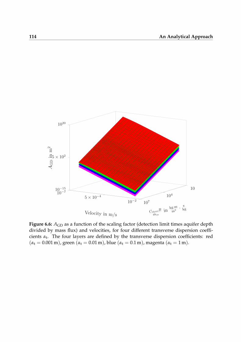
114 An Analytical Approach

CthresB

min

inkg·m

m3·

skg

Velocity in m/s

AGDin

m2

10

104

107

10−7

5× 10−4

10−2

10−15

5× 102

1020

Figure 6.6: AGD as a function of the scaling factor (detection limit times aquifer depthdivided by mass flux) and velocities, for four different transverse dispersion coeffi-cients αt. The four layers are defined by the transverse dispersion coefficients: red(αt = 0.001 m), green (αt = 0.01 m), blue (αt = 0.1 m), magenta (αt = 1 m).

6.4 Analysis of the Coordinating Factors 115

Low Detection Limit and Low Transverse Dispersion Pushes the

Optimal Monitoring Well Away from the Source

The optimal position for a monitoring well is the position where the plume has itslargest width

(Xopt =

(xopt, y0

), Equation 6.9

), because that position is most robust

against estimation errors in any of the parameters. As shown in Figure 6.7, the positionof this point is highly influenced by the detection limit. Low values in Cthres increasethe distance between Xopt and the source because the plume has more time to spreadlaterally until it is dissipated below the detection limit. The same effect can be seenfor small values in αt: a small transverse dilution leads to a very stretched plume thatreaches its largest width far away from the source.

Large Uncertainty in Spill Location Sharply Reduces AGD

The influence of the source location uncertainty diameter Ds on AGD is small until Ds

approaches wmax. The effect of Ds is much smaller than the influence of the transverse

αt = 0.001

αt = 0.01

αt = 0.1

αt = 1

CthresB

min

inkg·mm3 ·

skg

Xoptin

m

0 5× 106

107

10−5

100

105

Figure 6.7: X-position of the maximum width of the plume Xopt as a function of thefactor of detection limit, aquifer depth and mass flux for a constant velocity of 10−5

m/s. The set of curves is defined by four transverse dispersion coefficients (αt in m).

116 An Analytical Approach

dispersion or the detection limit (cf. Figure 6.8). However, for values of Ds close towmax, AGD strongly decreases. In the limiting case of Ds = wmax, just one point re-mains where 100% detection probability can be achieved and AGD shrinks to zero. Theremaining point is located at the point of largest plume width (Xopt, see Section 6.4 andFigure 6.7). Note that the maximum width of the plume wmax is independent of uncer-tainty in transverse dispersion and only the position of the maximum width changes inlongitudinal direction with different values in αt (cf. Equation 6.10 that is independentof DT).

Angular Uncertainties Require Close Monitoring

In the scenarios with angular uncertainty, we define Xmax to be the maximum dis-tance from the source where one can still achieve a 100% detection probability. Forinfinitesimal values of the limiting uncertainty angle β0, the limit of xmax is the tip

of the plume(

limβ0→0

xmax = xtip

)(cf. Figure 6.9). For high values of β0, the limit

αt = 0.001

αt = 0.01

αt = 0.1

αt = 1

Ds/2 in m

AGDin

m2

0 20 Rmax 40

103

104

105

106

107

108

109

Figure 6.8: AGD as a function of the uncertainty diameter Ds. In the limit Ds/2 =Rmax = wmax/2, AGD shrinks to zero. The set of curves is defined by four transversedispersion coefficients (αt in m).

6.5 Summary and Conclusions 117

of xmax is zero(

limβ0→±90

xmax = 0)

. The first ten degrees of uncertainty angle β0

(abs (β0) < 10) cause 99% of the total effect (please observe the logarithmic scale forxmax). For abs (β0) > 10, the changes in xmax are merely in the range of centimeters.xmax is very sensitive to changes in β0 for small values in αt because the maximumwidth of these plumes is far from the source. Increasing β0 just slightly already leadsto a strongly increased vertical shift of the plumes along the x-axis. Thus, AGD de-creases significantly.

Angular Uncertainties Lead to the Failure of Monitoring

Figure 6.10 clearly shows that AGD for uncertainty in ambient flow direction dramati-cally decreases with increasing angular uncertainty β0. This affects especially plumeswith small values in αt because the distances between the origin of the sources andthe positions where these plumes have their maximum width

(Xopt

)increase with de-

creasing αt (cf. Figure 6.7). These plumes are relatively thin, such that the sizes of AGD

are highly sensitive to changes in β0. With large values in β0, however, AGD becomesinfinitesimal for all considered plumes and exists only theoretically. Such small AGD

have no practical benefits, and a reliable monitoring is impossible.

6.5 Summary and Conclusions

In this chapter, I investigated the physical mechanisms and their uncertainties thatcontrol the optimal placement of monitoring wells. I considered the most simple case:A single monitoring well is positioned in order to observe whether or not a singlepossible point-source has emitted a contaminant plume or not. I developed analyticalsolutions for the optimal monitoring position and its robustness as functions of sev-eral parameters of interest: the radius of uncertainty in contaminant release location(x0, y0), the value of the depth-specific contaminant mass discharge min

B , the value ofambient flow velocity v and its uncertainty interval in angle β, the value of the de-tection limit Cthres, and the value of transverse dispersivity αt. The derived analyticalsolutions showed that

1. the area of guaranteed detection greatly increases with decreasing detection limitand transverse dispersion,

2. a low detection limit and low transverse dispersion pushes the optimal monitor-ing well away from the source,

3. a large uncertainty in spill location drastically reduces the area of guaranteeddetection,

118 An Analytical Approach

αt = 0.001

αt = 0.01

αt = 0.1

αt = 1

β0 in degree

xmaxin

m

0 30 60 9010−3

100

104

Figure 6.9: Intersection point xmax as a function of angular uncertainty ±β0 in ambientflow direction. For β0 = 0 the intersection point is at xmax = xtip. The set of curves isdefined by four different transverse dispersion coefficients (αt in m).

4. angular uncertainties require spatially close monitoring and spoil the robustnessof monitoring.

Because the solutions are provided closed form, it is easy to analyze the effects of thecontrolling factors and their uncertainty. That is, the solutions can be used

• to improve the fundamental understanding of controlling factors that influenceoptimal monitoring-well position and support (or enable) the inverse thinkingmentioned in the very beginning of this chapter.

• to provide decision support for evaluating and upgrading existing monitoringnetworks, acknowledging the inherent uncertainty through the evolvement ofdetection probabilities.

6.5 Summary and Conclusions 119

αt = 0.001

αt = 0.01

αt = 0.1

αt = 1

β0 in degree

AGDin

m2

0 30 60 9010−10

10−5

100

105

1010

Figure 6.10: AGD as a function of angular uncertainty ±β0 in ambient flow direc-tion. The set of curves is defined by four different transverse dispersion coefficients(αt in m).

Chapter 7

Insights from Practical Application

Parts of this chapter have been published in the Journal WATER RESOURCES RESEARCH

under the title Reconnecting Stochastic Methods with Hydrogeological Applications: A Util-

itarian Uncertainty Analysis and Risk Assessment Approach for the Design of Optimal Mon-

itoring Networks Bode et al. (2018b) [15]. I am reusing parts of the text and figuresfrom this publications by the kind permission of the publisher American GeophysicalUnion.

As already mentioned in Chapter 1, this work aims to develop simple-to-use meth-ods for hydrogeological problems in practice. The previous chapters all work towardsthis goal: I adjusted and simplified the optimization problem (Chapter 4), I developedfeasible concepts regarding the groundwater contaminant simulation for practical ap-plications (Chapter 5), and I developed simple analytical tools to evaluate optimizationresults under uncertainty (Chapter 6).

This chapter demonstrates that these methods and concepts can successfully be trans-ferred to practice by presenting select numerical results from the cooperation projectintroduced in Chapter 1. These results show that efficient, effective, and reliablemonitoring-design optimization is possible on real-world cases under computationallimitations and time constraints.

However, the transfer from academia to practitioners requires careful and effectivecommunication to ensure that data acquisition, data evaluation, and invested projectresources support the interests of both parties. The fact that communication is crucialin co-productions and collaborations between academics and practitioners has alreadybeen identified in literature related to stakeholder engagement [e.g., 2, 47]. Some com-mon problems in such collaborations are: the use of jargon; discipline-specific softwarewith steep learning curves; and other group-specific, implicit mindsets used by bothparties.

Therefore, in the second part of this chapter, I highlight important aspects of projectmanagement learned that led to a mutually successful project. The lessons learned aremuch more general than the specific project. I believe they will be useful for futurecollaborations between academic and industrial partners in the face of uncertainty for

7.1 Real Case 121

many hydrogeologic, hydrologic, and other environmental problems. Further liter-ature regarding challenges, benefits, and drawbacks related to stakeholder engage-ment in environmental modeling can be found in the reviews of Reed (2008) [133] andKrueger et al. (2012) [98]. The interested reader is also referred to the special issue Water

Governance, Stakeholder Engagement, and Sustainable Water Resources Management editedby Megdal et al. (2017) [114]. It gives a broad overview of recently published studieson stakeholder engagement related to the field of water resources management.

7.1 Real Case

The case study investigated here is based on the drinking-water well catchment ofthe Zweckverband Landeswasserversorgung (LW) in Stuttgart, Germany. The catchment islocated south-east of Stuttgart at the Swabian Jura and the Donauried. It has an area ofaround 300 km2. The geological composition of the catchment in vertical direction ischaracterized by five layers. A large area is dominated by a jura stratum (from north-west to south-east) that drops below tertiary molasse layers close to the productionwells. Above the molasse layers, there are gravel layers with a thickness of around8 − 10 m and a covering soil layer. Large parts of the jura stratum are karst aquifers.For water production, more than 200 pumping wells are grouped in eight well galleries(see purple squares in Figure 7.1), producing a maximum of 2.5 m3/s fresh water. Thecatchment produces about 40 × 106 m3 fresh water per year.

Within the catchment, more than 1,500 possible contamination sources could be iden-tified by the LW from which 143 were labeled as "relevant". These relevant sourceswere divided into three groups according to their subjective risk (cf. Section 5.4): "al-most tolerable", "medium", and "severe" sources (cf. green, yellow, and red dots inFigure 7.1).

7.1.1 Transport Simulation

The transport simulation is based on a three-dimensional flow field generated withModFlow and provided by the LW. It includes the five different geological layers de-scribed above. The different layer-specific and transport-relevant parameters can befound in Table 7.1. For transport simulation, the model domain is discretized with aregular grid (50m × 50m × 5m) and, in total, includes 77,589,720 cells. The catchmentoutline is approximated using more than 6,000,000 particles in the backward transportsimulation with RPTRW (cf. Section 2.3). Once the catchment was found, some morepossible contamination sources could be labeled as irrelevant (cf. Section 5.2). Thesewere either not within the calculated catchment, or could not hazard the productionwells, because of subcritical contaminant mass or too long travel times. In Figure 7.2,

122 Insights from Practical Application

N

0 km 21 km 42 km

0 km

20 km

40 km

1

Figure 7.1: Top view of the real-case model domain. The colored background arearepresents the groundwater level (downward gradient from yellow to turquoise). Pur-ple squares: production wells; Gray overlay: simulated well catchment; Colored dots:143 possible contamination sources that are irrelevant (gray), almost tolerable (green),medium (yellow), severe (red).

7.1 Real Case 123

these irrelevant possible sources are marked as gray dots. The number of relevantsources could be reduced to 120.

The forward transport simulation from the possible contamination sources was per-formed with PTRW (cf. Section 2.3) and 5000 particles per source. This simulation isthe basis of the multi-objective optimization (cf. Section 3.1) and defines the search areaof meaningful monitoring-well positions, i.e., positions where, in principle, a possiblecontamination source can be detected.

Altogether, the transport simulations needed around 50 hours on a single Intel Corei5-4590 CPU with a maximum frequency of 3.3GHz, and 32 GB RAM. While most ofthe simulation time was required for defining the catchment (41 hours), the forwardtransport simulation only needed nine hours.

7.1.2 Optimization

The optimization is based on the risk-prioritized optimization formulation introducedin Equation 5.9, with detection probability fdet and early-warning time utility fwarn

for each of the three risk classes. For the early-warning time utility function fwarn thethree user-defined values (cf. Section 3.2.2) are set to: the minimum desirable early-warning time tmin = 2 years, the corresponding early-warning time utility umin = 0.75,and the maximum desirable early-warning time tmax = 30 years. The cost function

fcost is split up in installation costs f(i)cost and operational cost f

(o)cost. The installation

costs f(i)cost requires a detailed drilling-cost map that was provided by the LW. Besides

the drilling costs, it also includes fixed installation costs (e.g., the planning-costs of a

monitoring well). The operational cost function f(o)cost is a summation of all operational

costs, i.e., sample drawing and sample analysis, averaged maintenance and repair costsof the planned monitoring wells, etc.. That is, the problem formulation includes eightobjective functions:

dopt = arg mind∈D

[f(r)det, f

(r)warn, f

(y)det , f

(y)warn, f

(g)det , f

(g)warn, f

(i)cost, f

(o)cost

]. (7.1)

Table 7.1: Transport relevant parameters

Layer Longitudinaldispersivity αℓ

Transversaldispersivity αt

Volumetricporosity Φv

Effectiveporosity Φe

1 20 1 0.15 0.152 20 1 0.035 0.0353 150 7.5 0.01 0.014 150 7.5 0.01 0.015 150 7.5 0.0003 0.0003

124 Insights from Practical Application

From the transport simulation and its spatial resolution, we obtain a set of 924,520 pos-sible monitoring-well positions (cf. gray overlay in Figure 7.2). The optimal reductionmethod introduced in Section 4.3.3, reduces these to 7,660 possible monitoring-wellpositions (white pluses in Figure 7.2). Please note that possible monitoring-wells alsohave a vertical component, not shown in Figure 7.2. Figure 7.2 is the top view of themodel domain and possible monitoring-well positions in vertical direction are pro-jected to the top. Hence, they cannot be visually distinguished in vertical direction.

The optimization was performed with the Borg MOEA (cf. Section 4.1.1). The de-fault settings for the genetic operators can be found in Table 4.4. The ǫ-box precisionwas set to AC1000 for installation costs, to AC100 for operational costs, and to 0.01 forall detection-probability and early-warning time utility functions. I used the linear-indexing representation introduced in Section 4.2.2. Each solution is defined by 121decision variables: 60 binary decision variables that define the number of actual mon-itoring wells, 60 integer variables that define the position of the monitoring wells, anda single decision variable that specifies the sampling frequency (one, four, 12, or 48times per year for all planned wells). So, overall, the actually reduced search space stillcontains ∼ 4.3 × 10151 possible monitoring-network designs.

On the hardware mentioned above, the reduction took approximately one hour andthe optimization took approximately four hours.

7.1.3 Results and Discussion

Figure 7.3 shows a selection of the obtained approximation set (black lines). All objec-tive values are normalized and their ideal value is one. While the early-warning timeutility and detection probability functions are between zero and one per definition, thetwo cost functions are normalized with the maximum values over all solutions. Here,the figure only shows 10% of the entire solutions, i.e., 5,591 out of 55,909 solutions,selected after the criterion of best compromise for detection probability for the threedifferent risk classes.

Figure 7.3 shows that the optimization algorithm was unable to find solutions with sat-isfying detection probabilities for almost tolerable (max. ∼ 45%) and for the medium(max. ∼ 60%) possible contamination sources. The maximum detection probability forsevere sources is at around 90%. However, analysis of the transport simulation showsthat without any limitation in the number of possible monitoring wells the maximumreachable detection probability values for this problem are 69% for almost tolerable,66% for medium, and 97% for severe possible contamination sources. That is, the dif-ferences between the actual goal attainment of the optimization and the maximumpossible values express the difficulty of the optimization problem.

The red line in Figure 7.3 represents the objective values of the monitoring networkthat is illustrated in Figure 7.2 as blue crosses. It is defined by 29 monitoring wells

7.1 Real Case 125

N

7 km 18 km 36 km

12 km

16 km

31 km

1

Figure 7.2: Detail of the top view from Figure 7.1. Gray overlay: possible monitoring-well positions; White pluses: remaining possible monitoring-well positions after opti-mal reduction (cf. Section Section 4.3.3); Blue crosses: exemplary optimized monitor-ing network; all other mark/colors: same as in Figure 7.1.

126 Insights from Practical Application

and provides a detection probability of 90% for the severe, 38% for the medium, and26% for the almost tolerable possible contamination sources. The early-warning timeutilities are between 0.01 and 0.04. The installation costs are around AC2.2 × 106and theoperational costs are AC3.2 × 105 per year. The high operational costs are caused by thehigh sampling frequency of 48 samples per year and monitoring well. This samplingfrequency is necessary because there are several possible contamination sources witha short visibility at the monitoring-well positions. With lower sampling frequencies,detection probability would fall for all sources.

Most of the monitoring wells form a barrier close to the production wells, wheremany possible contamination sources overlap. Especially, the group of sources at[18km, 15km] needs heavy monitoring by 2

3 of all monitoring wells. Some of the re-maining monitoring wells protect the production wells in a selective way, i.e., theymonitor in a one-to-one situation (e.g., at [12km, 21km] or the monitoring wells at[27km, 21km]).

Altogether, in absolute values, the presented monitoring network is expensive in in-stallation and operation. However, this problem formulation ignores already existingmonitoring wells that could be easily included by adapting the drilling-cost map (nocosts at positions with already existing monitoring wells). The detection probability ofsevere and medium sources can only be increased by increasing the sample frequency.Focusing only on the severe possible contamination sources could heavily reduce op-erational and installation costs because the number of relevant sources would dropfrom 120 to 22. The LW has run its own various versions of this optimization problemwith an earlier version of the methods developed here, released as a software packagecalled PROMETEUS. PROMETEUS was developed within the project together withthe DVGW introduced in Section 1.1. The results of the LW are published in the finalreport of this project [67].

As a conclusion, in this section, I exemplary showed that the methods introduced in theprevious chapters are serving the goal to enable water suppliers the use of academicconcepts regarding the optimization of monitoring networks under uncertainty. Re-sults show, that efficient and effective monitoring networks can be found in reasonablecomputing time (in total, 55 hours were needed for the entire process).

7.2 Communication Strategies

In this section, I present suggestions for how collaboration between the practical andthe academic sides can be improved on projects that include uncertainty as challenge.Three key strategies that emerged during the project (introduced in Chapter1) are em-phasized in the following subsections. All of them required frequent communication

7.2 Communication Strategies 127

f(i)cost f

(o)cost f

(g)warn f

(y)warn f

(r)warn f

(g)det f

(y)det f

(r)det

0

0.5

1

1

Figure 7.3: Selection of the Pareto-approximation set. X-axis: objective functions; Y-axis: normalized objective values (cost-values were normalized with the costs of themost expensive network); Black lines: non-dominated solutions; Red line: solutionillustrated in Figure 7.2 as blue crosses.

128 Insights from Practical Application

through meetings involving the entire project group or sub-groups comprised of, e.g.,only the operating engineers or only single water suppliers.

Speaking the Same Language Is Important

The biggest challenge and most important element in the collaboration was to developa common language. This language has to be developed from the beginning of theproject and has to be continually evolved as new challenges and opportunities arise.Clear communication is especially important for concepts related to uncertainty, risk,and optimality because common conceptions and intuitions often differ starkly fromscientific definitions in these realms. As a result, it can be important to state all defi-nitions, even those that may seem obvious, to avoid miscommunication. Our strategyduring the project was to maintain a close connection between the academic team andone water supply company that represented the practical side. The process involvedlong discussions, exacting explanations, translations, and interpretations; but, it re-sulted in glossaries that could be shared across the entire project group. The resultsfound rapid acceptance within the entire group because both practitioners and aca-demics were involved in their generation.

Good Visualization of Methods and Concepts Is Very Helpful

Whenever the project group developed or introduced a new method or concept, itwas important that it was explained clearly to every participant as quickly as possible.While a large body of literature focuses on visualization techniques of scientific data[e.g., 55, 81, 82], conceptual illustrations are strongly related to the problem; hence it isdifficult to develop general rules for designing them. However, simple and illustrativefigures (as simple as possible, as complex as necessary [e.g., 151]) were the most im-pactful medium for communicating new methods and concepts. An example of simpleand story-telling illustration is given in Figure 7.4 that shows the line-of-attack conceptintroduced in Section 5.6. A combined task force of one representative water supplierand some academic participants together created story-telling visualizations and il-lustrative flow charts to capture the key concept. The practitioners usually led thiseffort because they had direct knowledge of what would be accessible and informativeto other practitioners. The academic side helped to prioritize the most important as-pects of each idea that kept the analyses on solid scientific grounding. In the best case,these illustrations were intuitively understandable in such a way that they worked asanchors for the represented concepts after they were introduced and immensely sim-plified communication during the project.

7.2 Communication Strategies 129

Pos. con. sou.Pumping well

RepresentativesUrban areaIndustrial park

Monitoring wellFigure 7.4: Example of a story-telling illustration. The figure illustrates the line-of-attack concept to tackle the problem of unknown possible contamination sources. Theblue dots represent virtual contamination sources and the gray squares are the respec-tive monitoring network. The gray shadow illustrates the monitoring direction of thenetwork.

Finding the Same Objectives Supports the Collective

A strong collaboration results in a whole that is greater than the sum of its parts. Toachieve this, each group has to have its own motivations and objectives that drive theircontributions to the team effort. This statement, which applies at a technical level, alsoholds at the higher level of the overall purpose of the project. In the extreme, thepractical participants might be focused on developing less expensive, innovative toolsto design better monitoring networks. Meanwhile, the academic participants may bemost interested in gaining access to a large pool of real data to test their methods. Aswith all collaborations, much of the effort lies in aligning these differing motivations toleverage the strengths of each partner. We found that it was useful to acknowledge theseparate motivations of the partners but to work openly to define a joint objective ofdeveloping a useful and practical software with state-of-the-art methods and perspec-tives. This required relaxation of expectations on the academic side because purelyacademic methods could not always be applied feasibly. However, in some cases, thisrequired flexibility from the practitioners, who sometimes assume that seemingly com-plex methods were not worth the time or effort. Often, the academic partners made useof jointly-developed illustrations to communicate the methods under consideration.Interestingly, this tension led to balanced but innovative approaches, as described inSection 5.4. Ultimately, the shared overall objective was well served by the practical fil-

130 Insights from Practical Application

ter placed on the academic ideas and by the requirement that both sides work to find acommon language and compelling illustrations to understand all aspects of the project.This process further benefited from the diversity of the practical side, which includeddecision makers, field engineers, modelers and administrative employees for differentwater suppliers working in very different well catchments. Additionally, employeesfrom the ministry and representatives from the head organization (DVGW) partici-pated. Each of them brought different perspectives and placed different emphases onindividual technical problems, needs, and concerns.

In summary, during the project, communication was critical. I found the followingthree strategies to be most useful:

1. Terminology: The project group developed glossaries for uncertainty and riskterminology to ensure that we had a common language. This basic vocabu-lary minimized unnecessary misunderstandings and formed the foundation forbuilding common understanding as the group chose and developed more in-volved analyses later in the project.

2. Illustrations: The project group worked as small, collaborative, multidisciplinarygroups to create clear illustrations to visualize and understand concepts relatedto scientific analysis, uncertainties, and risks. These made it easy for everyoneinvolved to understand these concepts. The illustrations were critical for buildingsolid understanding of complex concepts across all partners. Importantly, thepractitioners led in the development of these illustrations because they were inthe best position to know whether a figure would communicate concepts clearlyto those who would use the software in practice.

3. Joint objectives: The project group recognized that each participant had differ-ent main goals when forming the team, but we committed to developing a jointobjective that we could all use to guide constructive collaboration.

The following three general conclusions may extend beyond this project:

1. Flexibility: Practitioners are aware of the uncertainty problem and have devel-oped strategies to conduct their operations under uncertainty. Academics donot need to explain uncertainty or convince practitioners to care about it. But,they must clearly explain why their methods add value to practitioners by betterdefining critical uncertainties. However, academics must understand that manyof their methods to quantify uncertainty are not feasible in practice because ofdata limitations or computational demands. Therefore, academics must be flex-ible in modifying and simplifying their approaches to provide the best possibleinsights within budgetary limits.

2. Direction: In some cases, the practitioners’ desired level of simplicity would re-quire unacceptable (from the viewpoint of academics) modifications of academic

7.2 Communication Strategies 131

methods. Then, it is incumbent upon academics to work with practitioners todevelop clear illustrations that can explain the need for the more advanced anal-yses. Both sides must approach this process openly, nudging toward a commonsolution and avoiding the temptation to demand simplicity or rigor.

3. Communication: The importance of communication cannot be overstated: frominitial efforts to develop common terminology, to the development of a joint ob-jective, to continually developing visual aides to ensure integrated understand-ing. This willingness to spend the time required to share ideas is the only wayto demonstrate the honesty, transparency, and mutual appreciation required toleverage each partner’s contributions toward a common goal. Each partner willbring unique strengths to the process, but communication is the quintessence ofa successful collaboration.

Chapter 8

Summary, Conclusions, and Outlook

In this chapter, I will summarize my contributions presented in this thesis (Section 8.1),and give some concluding remarks on what I have learned during the transfer of thedeveloped methods to practice (Section 8.2). In the final Section 8.3, I present someideas for further research that are based upon this thesis.

8.1 Summary

The overarching goal of this thesis was to develop appropriate concepts and computa-tionally efficient methods for the search of optimal monitoring networks in drinking-water well catchments. In most well catchments, many possible contamination sourcesendanger fresh-water aquifers and water supply wells. To control the emerging risk,monitoring networks are typically used, which track the groundwater quality prior toproduction. Finding optimal monitoring networks, however, is challenging becausetheir objectives are often manifold and competing. The three main objectives I consid-ered in this thesis were (1) to maximize the detection probability of spilled contamina-tion, (2) to maximize the early-warning time for water suppliers to provide sufficientreaction time for installing countermeasures, and (3) to minimize the overall costs ofthe monitoring network. Beyond the conceptualization for the optimization problem,objectives for the involved computational methods were (4) to be efficient, and (5) ro-bust against either statistical uncertainty, scenario uncertainty, or unknown unknowns.The work was strongly influenced by a project called Risk-Based Groundwater Monitor-

ing for Well Head Protection Areas together with the German Technical and Scientific Asso-

ciation for Gas and Water (DVGW) and national water-supply companies.

Within the four Chapters 3 to 6 that contains my original contributions, I approachedthe overall problem from different directions:

1. In Chapter 3, I formulated the multi-objective optimization problem and devel-oped the corresponding objective functions: detection probability, early-warningtime, and costs. I presented aggregation rules of the objective values, (1) if a mon-itoring network monitors more than a single possible contamination source, and(2) if the transport model is subject to predictive uncertainty and multiple scenar-ios or realizations are considered. In Chapter 3, I also developed two test cases:a zonation-based model, called Z_Based, that abstracts typically used models

8.1 Summary 133

from water-supply companies, and U_Protect, an urban source water protectiontest case that captures key complexities for real-world source water protection ingroundwater-based water supplies. In an exemplary discussion on U_Protect, Ishowed that the three considered objectives are in fact competing, and hence thatmulti-objective optimization is an appropriate approach to solve the optimizationproblem.

2. In Chapter 4, I investigated methods in detail for search improvements for multi-objective and discrete combinatorial optimization problems. I developed (1) anefficient and reliable search-space representation, the linear-indexing represen-tation, that can handle large decision spaces without significant computationallosses, and (2) I contributed a search space reduction method, the optimal reduc-tion, that provides speedy search while ensuring that the attained multi-objectivetrade-offs are high-quality approximations to the true Pareto-optimal solutions.

In the context of the U_Protect test case, I showed that both the linear-indexingrepresentation and the optimal reduction method clearly improved optimizationresults, compared to selected other representation and reduction methods, e.g.,binary representation and grid-based reduction.

The overarching conclusion is that, for discrete problems, linear-indexing repre-sentation is the key for a reliable and efficient optimization performance. Addi-tionally, when feasible, the proposed optimal reduction helps to improve qualityand end-point value of multi-objective analyses for the design of groundwatermonitoring systems for source water protection. These insights can be trans-ferred to a broad class of optimization problems. My results enable the feasibilityof multi-objective optimization on standard desktop computers in operationallyvalid runtimes.

3. In Chapter 5, I presented possible strategies to apply academic concepts in prac-tice such that they are frugal enough to run on standard personal computers, andthat they can be operated with realistically available data. These included strate-gies regarding the transport simulation, a qualitative risk-prioritization approachthat enables water suppliers to account for their own (subjective) fears againstpossible contamination sources, a strategy to minimize the effort for screeningareas with many possible contamination sources, and a risk model that repre-sents unknown possible contamination sources and enable an effective and ro-bust monitoring.

The main points I concluded in this chapter were (1) that Monte-Carlo simula-tions are not feasible to represent uncertainty in practice, and well-selected sce-narios should be preferred, (2) that a qualitative risk prioritization within the op-timization helps find cost-efficient monitoring networks, and (3) that unknownpossible contamination sources can be considered by a proper risk model. Over-all, the presented utilitarian approaches serve the goal to adopt computationally

134 Summary, Conclusions, and Outlook

demanding and data-hungry complex statistical methods for practical applica-tion.

4. In Chapter 6, I investigated the physical mechanisms and their uncertainties thatcontrol the optimal placement of monitoring wells. I considered the most simplecase: A single monitoring well is positioned in order to observe whether or nota single possible point-source has emitted a contaminant plume or not. I devel-oped analytical solutions for the optimal monitoring position and its robustnessas functions of several parameters of interest. Because the solutions are providedclosed form, it is easy to analyze the effects of the controlling factors and theiruncertainty. The solutions can be used to provide decision support for evaluat-ing and upgrading existing monitoring networks, acknowledging the inherentuncertainty through the evolvement of detection probabilities.

In Chapter 7, I applied the developed methods and strategies on a real case and pre-sented communication strategies for a successful collaboration between academia andindustry. The three main strategies found during the project with the DVGW andnational water suppliers were (1) that a clear terminology is key for a mutual under-standing, (2) that clear and story-telling illustrations help understand complex scien-tific concepts and methods regarding uncertainty analysis and risk assessment, and (3)that a joint objective between the collaboration partners guides the right direction ofthe project.

From the project, I found three general conclusions regarding collaborations betweenacademia and practice. First, practitioners are aware of the uncertainty problem, butthey do not have instruments and methods to properly tackle it. The academic meth-ods, however, are often not feasible and need modifications in data hungriness andcomputational efficiency. Second, too much simplification on complex scientific meth-ods is not constructive and academics and practitioners need to find a trade-off solu-tion between simplicity and rigor. Finally and most importantly, communication is thequintessence of a successful collaboration.

8.2 Conclusions From Transfer to Practice

In this section, I will make some general conclusions I have learned during the collab-oration within the DVGW project. Parts of this section have been published in Bodeet al. (2018b) [15].

Collaboration It can be useful to recognize that the process of jointly defining anacademic/practical partnership is a multi-objective optimization exercise between sci-entific priorities and practical utility. There is a useful creative tension that arises when

8.3 Outlook 135

practitioners demand simple approaches and academics are required to explain andadvocate for more advanced analyses. The process winnows potentially expensive ap-proaches with little practical benefit while forcing all partners to clearly understandthe relevance of all aspects of the study. The key point is that academics should listento the needs of the users, design the analyses to provide them with useful informationand provide tools to help them to define their preferences and to integrate them withthe science.

Optimization Multi-objective optimization is a powerful concept, but it needs to becommunicated clearly as a strength for decision makers to achieve practical buy-in.

Risk From the practical side, approaches to risk assessment that stressed clarity, sim-plicity, and applicability were preferred; in general, qualitative risk assessment waspreferred to rigorous, but less practical, quantitative approaches. In some cases, theonly feasible risk analysis will be fully qualitative, based on subjective public concernsand expert judgments of stakeholders. This will require thoughtful collaboration todefine the appropriate model ensemble and to decide how to apply it to decision mak-ing.

8.3 Outlook

In the following, I present some ideas for further research that are built upon my thesis.

• In Chapter 3, I introduced the objective-function formulation of the cost functionthat is a simple summation of arising expenses and does not consider consequen-tial costs. I argued that the consequential costs are one of the main motivation forwater suppliers to invest in optimal monitoring networks, hence there is no needfor considering these costs. In practice, however, politicians, stakeholders, anddecision-makers often must be convinced to invest in such networks who are notdirectly involved in the daily business of water-providing companies. Then, con-sidering and modeling consequential costs can be very persuading and could bea necessary step to help protect fresh-water aquifers.

• The three main objectives of the monitoring networks to be fulfilled are detectionprobability, early-warning time, and costs. The optimized networks should con-trol the risk coming from the identified possible contamination sources. In caseof a groundwater contamination and a detection by a monitoring well, the waterprovider is warned but has no information about the contamination source. In fu-ture work, the formulated optimization problem could be extended by an objec-tive function that evaluates the ability of monitoring-well locations and monitor-ing networks to identify the actual contamination source. Monitoring networks

136 Summary, Conclusions, and Outlook

that are designed to also consider source identification would minimize the con-taminated area, hence would minimize remediation costs of the contaminatedsoil.

• In Chapters 3 and Chapter 4, I investigated optimization under uncertainty.When considering uncertainty, the stability of the optimization strongly dependson the aggregation function over the ensemble of scenarios/realizations. Here,it would be interesting to determine, how much uncertainty can be tolerated bythe optimization problem and the different aggregation functions until the opti-mization collapses. The goal would be to find optimal trade-offs between robustoptimization and uncertainty reduction, and the question is: when should the de-cision maker invest in uncertainty reduction and how long can the optimizationstill find satisfying results under increasing uncertainty?

• In Chapter 4, I presented the linear-indexing representation of the search space.The corresponding index vector emulates the actual search space and simplifiesthe sampling and mutation/recombination step during the optimization. Therandom sampling is based on a uniform distribution. The idea for further re-search is to sort the elements of the index vector by characteristics of their ob-jective values via, e.g., k-means clustering, and to provide multiple additionalsampling distributions that are related to these different clusters. The samplingdistribution used for a solution could be assigned by an additional decision vari-able and must be the same in the mutation/recombination step for a definednumber of function evaluations. Ongoing research already showed that this ideacan increase the diversity of the Pareto-front approximation by better exploringthe edges of the front.

• In Chapter 5, I stated that well-selected scenarios are better suited than Monte-Carlo simulation in practice for uncertainty representation. Although I clearlydefined what exactly is meant by well-selected, it might be difficult for watersuppliers to find well-selected scenarios that satisfy the definition. Therefore,ongoing research should be invested in developing guidelines for smart and easyscenario selections.

• Chapter 6 provides analytical solutions for optimal monitoring location underuncertainty for single possible contamination sources. These solutions could beextended to multiple possible contamination sources.

• Overall, for practical application, it would be exceptional to have a tool that eval-uates the quality of sequentially built monitoring networks to better guide theeffective installation. Water providers would clearly benefit from it since theycould investigate, which monitoring well brings the most gain in quality. Thus,they could prioritize the sequence of installation.

Appendix A

Analytical Solutions

A.1 Derivation of the 2D Steady-State

Advection-Dispersion Equation

We consider the advection-dispersion equation for uniform and parallel flow in x-direction and a uniform dispersion tensor D:

∂C

∂t+ vx · ∇C −∇ · (D∇C) = 0 , (A.1)

with concentration C, time t and velocity vx (v in the following). For a two-dimensional, steady-state case, Equation A.1 simplifies to

v∂C

∂x− Dxx

∂2C

∂x2 − Dyy∂2C

∂y2 = 0 . (A.2)

As explained in Section 2.2, we can neglect longitudinal dispersion and the termDxx

∂2C∂x2 in Equation A.2 vanishes. Then, we can apply a transformation of coordinates,

substituting x by travel time τ: x = vτ and x turns into a time coordinate. The changedEquation A.2

∂C

∂τ− Dyy

∂2C

∂y2 = 0 (A.3)

is the one-dimensional diffusion equation, Fick’s second law, respectively. For an infi-nite domain, the solution for Equation A.3 is

C (y, τ) =c1√

τexp

(− y2

4Dyyτ

), (A.4)

with the boundary conditionlim

y→±∞C (τ, y) = 0

and c1 as an arbitrary constant [27]. With the initial condition C (τ = 0, y) = minv δ (y)

with the Dirac-Delta Function [41], in Equation A.4 the constant c1 equals min

v√

4πDyyτ.

With the inverse transformation from τ to x, the final solution of Equation A.2 is

C (x, y) =min

B√

4πDyyvxexp

(− y2v

4Dyyx

). (A.5)

The division by the aquifer depth B highlights that this solution is depth-averaged. Inthe following, the transverse dispersion Dyy is denoted as DT.

Appendix B

Derivations for Chapter 6

B.1 Derivation of AGD

In this section, I derive the antiderivative of ythres with respect to x in Equation 6.6. Asintegration bounds, we use x1 = 0 and x2 = xtip. Since ythres is symmetric, we candouble the calculated area:

AGD = 2 ·∫ x2

x1

ythres (x) dx (B.1)

with

ythres =

√−4DT

vx · ln

(CthresB

min·√

4πvDTx

). (B.2)

Using

ψ =−4DT

v(B.3)

and

ρ =CthresB

min·√

4πvDT (B.4)

Equation B.2 can be simplified and the antiderivative can be expressed as

AGD = 2√

ψ ·∫ x2

x1

√x ·(

ln (ρ) +12

ln (x)

)dx . (B.5)

This integral can be simplified by substituting

x = exp(

23

z2)· 1

ρ2

and hence

dx = exp(

23

z2)

z · 43ρ2 dz

to

AGD = 2√

ψ · 4

332

1ρ3 ·

∫ z2

z1

exp(

z2)· z2dz . (B.6)

Considering only the integral∫

exp(z2)· z2dz we can use partial integration

(∫

uv′dz = uv −∫

u′vdz) with u = z2 and v′ = exp(z2). While the derivative of u = z2

B.1 Derivation of AGD 139

is simple to solve (u′ = 2z), we can use the definition of the imaginary error functionto solve the integral of exp

(z2). The imaginary error function [e.g., 123] is defined as

erfi (z) = −i · erf (iz) =2√π

∫ z

0exp

(x2)

dx .

With that,∫

exp(z2)

dz =√

π2 erfi (z) + const. and we can solve the integral from Equa-

tion B.6:∫ z2

z1

exp(

z2)· z2dz =

[√π

2z2 erfi (z)

]z2

z1

−√

π∫ z2

z1

z erfi (z) dz . (B.7)

To solve Equation B.7 we can again apply partial integration with u = z (u′ = 1) andv′ = erfi (z). The antiderivative of the error function can be found in Abramowitz andStegun (1965) [1]:

∫erf (x) dx = x erf (x) +

1√π

exp(−x2

)+ const.

We still have to transform v =∫

erfi (z) dz to v = −∫

erf (t) dt with t = iz. With that,

v = z erfi (z)− exp(z2)√π

+ const. and

∫ z2

z1

z erfi (z) dz =

[12

z2 erfi (z)− 12√

πz exp

(z2)+

14

erfi (z)

]z2

z1

. (B.8)

Putting all together yields

AGD =2√

ψ · 4

332

1ρ3

∫ z2

z1

exp(

z2)· z2dz

=2√

ψ · 1

332

1ρ3

[(2z · exp

(z2)−√

π · erfi (z))]z2

z1, (B.9)

withz1,2 =

√3 ln (ρ) + 3 ln

(√x0,1)

. (B.10)

For solving the integral in Equation 6.6, we can summarize a constant factor γ:

γ =

(min

CthresB√

3π

)3 1v2DT

.

and calculate the integration bounds z1 and z2. Inserting x1 = 0 and x2 = xtip inEquation B.10 leads to z1 (x = 0) =

√−∞ = i∞ and z2(x = xtip

)= 0, respectively.

For the sake of readability, xtip is defined as

xtip =

(min

CthresB

1√4πvDT

)2

.

140 Derivations for Chapter 6

With that, AGD can be written as

AGD = γi ·[2x exp

(x2)−√

π · erfi (x)]z2

z1. (B.11)

Inserting the integration bounds leads to the final results AGD = AGD (z2)− AGD (z1):

AGD =∣∣−γ ·

√π∣∣ . (B.12)

B.2 Derivation of the Integration Limits for AGD

Considering Uncertainty in Spill Location

To solve the integral in Equation 6.11, we need to find the roots of Equation 6.12. Weare starting again with Equation B.2, simplified using ψ and ρ (Equations B.3 and B.4).Instead of using the uncertainty diameter Ds from Equation 6.12, now we are using ageneral shift y0:

ythres (x)− y0 = 0 . (B.13)

Inserting ythres into Equation B.13 yields

y20 − ψ (x − x0)

(ln (ρ) + ln

(√x − x0

))= 0 , (B.14)

with the spill location (x0, y0). Rearranging Equation B.14 yields

(x − x0)(

ln(

ρ2)+ ln (x − x0)

)− 2y2

0

ψ= 0 . (B.15)

Multiplying Equation B.15 with ρ2 and rearranging yields

(x − x0) ρ2(

ln(

ρ2)+ ln (x − x0)

)=

2y20ρ2

ψ. (B.16)

Equation B.16 can be also expressed as:

exp(

ln (x − x0) + ln(

ρ2)) (

ln(

ρ2)+ ln (x − x0)

)=

2y20ρ2

ψ, (B.17)

and we can apply the Lambert W function W (·) [e.g., 25]. It has the property that fora = b exp (b) the function is W (a) = b. When using the Lambert W function, we get

W

(2y2

0ρ2

ψ

)= ln (x − x0) + ln

(ρ2)

. (B.18)

Finally, in Equation B.16 the term ln(ρ2)+ ln (x − x0) can be substituted by Equa-

tion B.18 and the roots x1,2 are:

x1,2 =2y2

0

ψ Wj

(2y2

0ρ2

ψ

) + x0 , (B.19)

with j ∈ −1, 0.

B.3 Derivation of the Integration Limits for AGD Considering Uncertainty inAmbient Flow Direction 141

B.3 Derivation of the Integration Limits for AGD

Considering Uncertainty in Ambient Flow Direction

In order to calculate the integral in Equation 6.17, we need to find the intersectionpoint Xint in Figure 6.4. Again, we start with Equation B.2, simplified using ψ and ρ

(Equations B.3 and B.4) and now look for the roots of

ythres (x)− tan (β) x = 0 , (B.20)

with the uncertainty angle β. Rearranging Equation B.20 yields

x2 − ψ ln (ρ)

tan2 (β)x − ψ

2 tan2 (β)x ln (x) = 0 . (B.21)

Since we are not interested in the trivial solution x = 0 we only consider the equation

x − ψ ln (ρ)

tan2 (β)− ψ

2 tan2 (β)ln (x) = 0 . (B.22)

Equation B.22 can be rearranged to

−2 tan2 (β)

ψexp (ln (x)) = − ln

(xρ2)

. (B.23)

Multiplying Equation B.23 with exp(− ln

(xρ2))

yields

− 2 tan2 (β)

ψexp (ln (x)) exp

(− ln

(xρ2))

=

− ln(

xρ2)

exp(− ln

(xρ2))

. (B.24)

Equation B.24 can be also expressed as:

−2 tan2 (β)

ψ

1ρ2 = − ln

(xρ2)

exp(− ln

(xρ2))

, (B.25)

and we can again apply the Lambert W function W (·):

W(−2 tan2 (β)

ψ

1ρ2

)= − ln

(xρ2)

. (B.26)

Finally, in Equation B.23 the term − ln(

xρ2)

can be substituted by Equation B.26:

x = − ψ

2 tan2 (β)W(−2 tan2 (β)

ψ

1ρ2

). (B.27)

142 Derivations for Chapter 6

B.4 Why it is Appropriate to Only Consider Uncertainty

in Transverse Direction to the Flow of the Spill

Location

In Section 6.3 we substitute the ΩU-circle by uncertainty in transverse direction to theflow. Here, I show why this substitution is valid without losses. We are starting withEquation B.19 (this equation calculates the integration limits for AGD considering un-certainty in spill location (cf. Section 6.3)) and substitute the spill location (x0, y0) inpolar coordinates for the parameterized circle: x0 = r · cos (α) and y0 = r · sin (α).With that, the roots x1,2 depend only on the angle α, assuming the radius r of the circleis known and constant:

x1,2 (α) =2r2 sin2 (α)

ψ Wj

(2r2 sin2(α)

ψ ρ2) + r · cos (α) , (B.28)

with j ∈ −1, 0. Next, we take the derivative of Equation B.28 with re-spect to α, using the quotient rule and the derivative for the Lambert W function(

dW(x)dx = W(x)

x(1+W(x)), for x > − 1

e ⇒ j = 0)

[cf. 25]:

∂x1,2 (α)

∂α=

2r2 sin (2α)

ψ(

1 + W0

(2r2 sin2(α)

ψ ρ2)) − r sin (α) . (B.29)

The next step is to find the roots of Equation B.29:

2r2 sin (2α)

ψ(

1 + W0

(2r2 sin2(α)

ψ ρ2)) − r sin (α) = 0 . (B.30)

This cannot be solved analytically because we still have a sin (α) in the argument of theLambert W function. However, a parametric study with Equations B.29 and B.30 over

r ∈[0, Ds

2

]is shown in Figure B.1 and B.2. Here, we can see that the combinations of

r = Ds2 and α = ±90 are the limiting cases of AGD and the ΩU-circle can be represented

appropriately by uncertainty transverse to the direction of flow.

B.4 Why it is Appropriate to Only Consider Uncertainty in Transverse Direction tothe Flow of the Spill Location 143

α in degree

x1,2(α

)=

0

0 30 60 90 120 150 1800

xopt

xtip

2

xtip

Figure B.1: Intersection of the plume outlines (ythres (x)) and the x-axis over startingpositions α of the plumes on the edges of ΩU parametrized as a circle. The startingpositions are limited to the outline of a circle that has a radius r ≤ Ds

2 . The set of curves

(black) is defined by varying values of r ∈[0, Ds

2

]. The red line illustrates the result

for r = Ds2 . The vertical blue line illustrates that the extreme values of all curves are

independent of r and occur for α = 90.

144 Derivations for Chapter 6

α in degree

∂x1,2(α

)∂α

0 30 60 90 120 150 180−106

0

106

Figure B.2: The derivative of root-function shown in Figure B.1 over the angle α. The

set of curves (black) is defined by varying values of r ∈[0, Ds

2

]. The red line illustrates

the result for r = Ds2 , that is, the uncertainty in spill location where only one over-

lapping point of all possible plumes exists that evolve from the edges of the relatedΩU-circle.

Bibliography

[1] Abramowitz, M. and Stegun, I. A. (1965). Handbook of Mathematical Functions With

Formulas, Graphs, and Mathematical Tables. Dover Books on Mathematics, New York,9 edition.

[2] Allen, E., Kruger, C., Leung, F.-Y., and Stephens, J. C. (2013). Diverse Perceptions ofStakeholder Engagement within an Environmental Modeling Research Team. Jour-

nal of Environmental Studies and Sciences, 3(3):343–356.

[3] Allen, R. M. and Kanamori, H. (2003). The potential for earthquake early warningin southern California. Science (New York, N.Y.), 300(5620):786–789.

[4] Aller, L., Bennet, T., Lher, J., and Petty, R. (1987). DRASTIC A standardized systemfor evaluating groundwater pollution potencial using hydrogeologic setting. U.S.

EPA Report 600/2-87-035 Ada Oklahoma., 29(1):23–37.

[5] Babbar, M. and Minsker, B. S. (2006). Groundwater Remediation Design UsingMultiscale Genetic Algorithms. Journal of Water Resources Planning and Management,132(5):341–350.

[6] Bean, J. C. (1994). Genetic Algorithms and Random Keys for Sequencing and Op-timization. ORSA Journal on Computing, 6(2):154–160.

[7] Bear, J. (1961). Some experiments in dispersion. Journal of Geophysical Research,66(8):2455–2467.

[8] Bear, J. (1972). Dynamics of Fluids in Porous Media. Dover Publications.

[9] Benson, A. K., Payne, K. L., and Stubben, M. A. (1997). Mapping groundwatercontamination using dc resistivity and VLF geophysical methods - A case study.Geophysics, 62(1):80–86.

[10] Bode, F., Binning, P. J., and Nowak, W. (2013). What Factors Coordinate the Op-timal Position of a Single Monitoring Well Down Gradient of a Hazardous Site. InAGU Fall Meeting 2013, Abstract: H21I-1175, San Francisco, CA, USA.

[11] Bode, F., Binning, P. J., and Nowak, W. (2014a). Enhanced Multi-objective Op-timization of Groundwater Monitoring Networks. In NGWA Groundwater Summit

2014, Denver, CO, USA.

[12] Bode, F., Binning, P. J., and Nowak, W. (2014b). Multi-Objective Optimizationof Groundwater Monitoring Networks: Computational Costs vs. Optimization Ac-curacy. In XX. International Conference on Computational Methods in Water Resources

(CMWR), Stuttgart, Germany.

[13] Bode, F., Binning, P. J., and Nowak, W. (2018a). An Analytical Approach forPositioning a Single Monitoring Well to Reliably Detect Point-Source ContaminantPlumes. Manuscript, In Prepara.

[14] Bode, F., Emmert, M., Zigelli, N., and Nowak, W. (2017). Optimale Grund-wassermessstellennetze: Multi-kriterielle Optimierung als Entscheidungshilfe. gwf

Wasser+Abwasser, 158:111–121.

[15] Bode, F., Ferré, T., Zigelli, N., Emmert, M., and Nowak, W. (2018b). ReconnectingStochastic Methods with Hydrogeological Applications: A Utilitarian UncertaintyAnalysis and Risk Assessment Approach for the Design of Optimal Monitoring Net-works. Water Resources Research.

[16] Bode, F., Loschko, M., and Nowak, W. (2014c). A Risk-Based Multi-Objective Op-timization Concept for Early-Warning Monitoring Networks. In AGU Fall Meeting

2014, Abstract: H23K-1023, San Francisco, CA, USA.

[17] Bode, F., Loschko, M., and Nowak, W. (2015). How to Decide? Multi-ObjectiveEarly-Warning Monitoring Networks for Water Suppliers. In EGU General Assembly

2015, Geophysical Research Abstracts 17: EGU2015-9270, Vienna, Austria.

[18] Bode, F. and Nowak, W. (2013). Optimizing early-warning monitoring systemsfor improved drinking water resource protection. In NUPUS, Bergen, Norway.

[19] Bode, F., Nowak, W., and Loschko, M. (2016a). Optimization for Early-Warning Monitoring Networks in Well Catchments Should Be Multi-objective, Risk-Prioritized and Robust Against Uncertainty. Transport in Porous Media, 114(2):261–281.

[20] Bode, F., Nowak, W., and Reed, Patrick. M. Reuschen, S. (2016b). Putting Manin the Machine: Exploiting Expertise to Enhance Multiobjective Design of WaterSupply Monitoring Network. In AGU Fall Meeting 2016, Abstract: H51A-1413, SanFrancisco, CA, USA.

[21] Bode, F., Reed, P. M., Reuschen, S., and Nowak, W. (2018c). Search Space Repre-sentation and Reduction Methods to Enhance Multi-Objective Water Supply Moni-toring Design. Water Resources Research, Submitted.

[22] Bode, F. and Reuschen, Sebastian Nowak, W. (2015). Never Use the CompleteSearch Space: A Concept to Enhance the Optimization Procedure for MonitoringNetworks. In AGU Fall Meeting 2015, Abstract: IN11B-1774, San Francisco, CA, USA.

[23] Bosman, P. and Thierens, D. (2003). The balance between proximity and diversityin multiobjective evolutionary algorithms. IEEE Transactions on Evolutionary Compu-

tation, 7(2):174–188.

[24] Cerny, V. (1985). Thermodynamical approach to the traveling salesman problem:An efficient simulation algorithm. Journal of Optimization Theory and Applications,45(1):41–51.

[25] Corless, R. M., Gonnet, G. H., Hare, D. E. G., Jeffrey, D. J., and Knuth, D. E. (1996).On the LambertW function. Advances in Computational Mathematics, 5(1):329–359.

[26] Cox, L. A. T. (2008). What’s Wrong with Risk Matrices? Risk Analysis, 28(2):497–512.

[27] Crank, J. (1979). The mathematics of diffusion. Oxford University Press.

[28] Cushman, D. J., Driver, K. S., and Ball, S. D. (2001). Risk assessment for envi-ronmental contamination: an overview of the fundamentals and application of riskassessment at contaminated sites. Canadian Journal of Civil Engineering, 28(S1):155–162.

[29] Dantzig, G., Orden, A., and Wolfe, P. (1955). The generalized simplex methodfor minimizing a linear form under linear inequality restraints. Pacific Journal of

Mathematics, 5(2):183–195.

[30] Davison, A., Howard, G., Stevens, M., Callan, P., Fewtrell, L., Deere, D., Bartram,J., World Health Organization. Water, S., and Team, H. (2005). Water safety plans:

managing drinking-water quality from catchment to consumer. Geneva: World HealthOrganization.

[31] Deb, K. (2001). Multi-Objective Optimization using Evolutionary Algorithms. JohnWiley & Sons, Chichester, UK.

[32] Deb, K. and Agrawal, R. B. (1994). Simulated Binary Crossover for ContinuousSearch Space. Complex Systems, 9:1–34.

[33] Deb, K., Agrawal, S., Pratap, A., and Meyarivan, T. (2000). A Fast Elitist Non-dominated Sorting Genetic Algorithm for Multi-objective Optimization: NSGA-II.In Parallel Problem Solving from Nature PPSN VI, pages 849–858. Springer.

[34] Deb, K., Joshi, D., and Anand, A. (2002a). Real-coded evolutionary algorithmswith parent-centric recombination. In Proceedings of the 2002 Congress on Evolutionary

Computation. CEC’02 (Cat. No.02TH8600), volume 1, pages 61–66. IEEE.

[35] Deb, K., Mohan, M., and Mishra, S. (2003). A fast multi-objective evolutionaryalgorithm for finding well-spread pareto-optimal solutions. Technical report, Kan-GAL, Kanpur, India.

[36] Deb, K., Pratab, S., Agarwal, S., and Meyarivan, T. (2002b). A Fast and ElitistMultiobjective Genetic Algorithm: NGSA-II. IEEE Transactions on Evolutionary Com-

puting, 6(2):182–197.

[37] Deb, K. and Sachin, J. (2002). Running Performance Metrics for EvolutionaryMulti-Objective Optimization. Technical report, KanGAL, Kanpur, India.

[38] Deuflhard, P. (2011). Newton Methods for Nonlinear Problems, volume 35 of Springer

Series in Computational Mathematics. Springer Berlin Heidelberg, Berlin, Heidelberg.

[39] Diersch, H.-J. G. (2014). FEFLOW: Finite Element Modeling of Flow, Mass and Heat

Transport in Porous and Fractured Media. Springer Science & Business Media.

[40] Dietrich, C. R. and Newsam, G. N. (1993). A fast and exact method for multi-dimensional gaussian stochastic simulations. Water Resources Research, 29(8):2861–2869.

[41] Dirac, P. A. M. (1958). The Principles of Quantum Mechanics. Oxford Science Publi-cations, 4 edition.

[42] Doherty, J. (2003). Ground Water Model Calibration Using Pilot Points and Regu-larization. Groundwater, 41(2):170–177.

[43] Dorigo, M. (1992). Optimization, learning and natural algorithms. Ph. d. thesis, Po-litecnico di Milano, Italy.

[44] Dossing Overheu, N., Tuxen, N., Flyvbjerg, J., Aabling, J., Andersen, J. A., Peder-sen, J. K., Thyregod, T., Binning, P. J., and Bjerg, P. L. (2013). Risk-based prioritisationof ground water threatening point sources at catchment and regional scale. Aqua-

ConSoil 2013 - Programme and Book of Abstracts, 485:171–172.

[45] DVGW (2003). Messnetze zur Überwachung der Grundwasserbeschaffenheit inWassergewinnungsgebieten. Technische Regel - DVGW W 108.

[46] DVGW (2006). Richtlinien für Trinkwasserschutzgebiete; Teil 1: Schutzgebiete fürGrundwasser. Technische Regel - DVGW W 101.

[47] Eden, S., Megdal, S., Shamir, E., Chief, K., and Mott Lacroix, K. (2016). Openingthe Black Box: Using a Hydrological Model to Link Stakeholder Engagement withGroundwater Management. Water, 8(5):216.

[48] Emmert, M., Zigelli, N., Haakh, F., Bode, F., and Nowak, W. (2016). RisikobasiertesGrundwassermonitoring für Wasserschutzgegiebte. energie - wasser-praxis, 8.

[49] Enzenhoefer, R. (2014). Risk quantification and management in water production and

supply systems. Dissertation, University of Stuttgart.

[50] Enzenhoefer, R., Binning, P., and Nowak, W. (2015). STakeholder-Objective RiskModel (STORM): Determining the aggregated risk of multiple contaminant hazardsin groundwater well catchments. Advances in Water Resources, 83:160–175.

[51] Enzenhoefer, R., Bunk, T., and Nowak, W. (2014). Nine Steps to Risk-InformedWellhead Protection and Management: A Case Study. Groundwater, 52(S1):161–174.

[52] Enzenhoefer, R., Nowak, W., and Helmig, R. (2012). Probabilistic exposure riskassessment with advective-dispersive well vulnerability criteria. Advances in Water

Resources, 36:121–132.

[53] EU (2018). Safer drinking water for all Europeans. European Commission - Press

release, IP/18/429.

[54] Faber, M. H. and Maes, M. a. (2003). Modeling of Risk Perception in EngineeringDecision Analysis. In Proceedings 11th IFIP WG7.5 Working Conference on Reliability

and Optimization of Structural Systems, volume 7, pages 113–122.

[55] Fayyad, U., Grinstein, G. G., and Wierse, A. (2002). Information Visualization in

Data Mining and Knowledge Discovery. Morgan Kaufmann Publishers, AcademicPress.

[56] Fernàndez-Garcia, D. and Sanchez-Vila, X. (2011). Optimal reconstruction of con-centrations, gradients and reaction rates from particle distributions. Journal of Con-

taminant Hydrology, 120-121:99–114.

[57] Folks, J. and Chhikara, R. (1978). The Inverse Gaussian Distribution and Its Sta-tistical Application–A Review. Journal of the Royal Statistical Society. Series B (Method-

ological), 40(3):263–289.

[58] Fonseca, C. M. and Fleming, P. J. (1993). Genetic Algorithms for MultiobjectiveOptimization: Formulation, Discussion and Generalization. Icga, 93(July):416–423.

[59] Freeze, R. A. (1975). A stochastic-conceptual analysis of one-dimensional ground-water flow in nonuniform homogeneous media. Water Resources Research, 11(5):725–741.

[60] Frind, E., Molson, J., and Rudolph, D. (2006). Well Vulnerability: A QuantitativeApproach for Source Water Protection. Groundwater, 44(5):732–742.

[61] Gelhar, L. W. and Axness, C. L. (1983). Three-dimensional stochastic analysis ofmacrodispersion in aquifers. Water Resources Research, 19(1).

[62] Glover, F. (1986). Future paths for integer programming and links to artificialintelligence. Computers & Operations Research, 13(5):533–549.

[63] Goldberg, D. E. (1989). Genetic Algorithms in Search, Optimization, and Machine

Learning. Addison Wesley Pub Co Inc.

[64] Goldberg, D. E., Korb, B., and Deb, K. (1989). Messy Genetic Algorithms: Motiva-tion, Analysis, and First Results. Engineering, 3:493–530.

[65] Gómez-Hernández, J. J. and Gorelick, S. M. (1989). Effective groundwatermodel parameter values: Influence of spatial variability of hydraulic conductivity,leakance, and recharge. Water Resources Research, 25(3):405–419.

[66] Gorelick, S. M., Evans, B., and Remson, I. (1983). Identifying sources of ground-water pollution: An optimization approach. Water Resources Research, 19(3):779–790.

[67] Haakh, F., Heß, C., Kaupe, M., Ries, J., and Nowak, W. (2016). Abschlussbericht -Risikobasiertes Grundwassermonitoring für Wasserschutzgebiete. Technical report,DVGW e.V.

[68] Hadka, D. and Reed, P. (2012). Diagnostic Assessment of Search Controls and Fail-ure Modes in Many-Objective Evolutionary Optimization. Evolutionary Computation,20(3):423–452.

[69] Hadka, D. and Reed, P. (2013). Borg: An Auto-Adaptive Many-Objective Evolu-tionary Computing Framework. Evolutionary Computation, 21(2):231–259.

[70] Hadka, D. and Reed, P. (2015). Large-scale parallelization of the Borg multiobjec-tive evolutionary algorithm to enhance the management of complex environmentalsystems. Environmental Modelling & Software, 69:353–369.

[71] Hajela, P. and Lin, C. Y. (1992). Genetic search strategies in multicriterion optimaldesign. Structural Optimization, 4(2):99–107.

[72] Halton, J. H. (1970). A Retrospective and Prospective Survey of the Monte CarloMethod. SIAM Review, 12(1):1–63.

[73] Ham, P. A., Schotting, R. J., Prommer, H., and Davis, G. B. (2004). Effects of hy-drodynamic dispersion on plume lengths for instantaneous bimolecular reactions.Advances in Water Resources, 27(8):803–813.

[74] Harbaugh, A. W. (2005). MODFLOW-2005, The U.S. Geological Survey ModularGround-Water Model - the Ground-Water Flow Process. In 6. Modeling techniques,chapter A16. US Geological Survey Reston, Reston, Virginia, USA.

[75] Harik, G. R. and Lobo, F. G. (1999). A parameter-less genetic algorithm. In Pro-

ceedings of the 1st Annual Conference on Genetic and Evolutionary Computation-Volume

1, pages 258–265. Morgan Kaufmann Publishers Inc.

[76] Hartigan, J. A. (1975). Clustering Algorithms. John Wiley & Sons.

[77] Harvey, C. F. and Gorelick, S. M. (1995). Temporal Moment-Generating Equations:Modeling Transport and Mass Transfer in Heterogeneous Aquifers. Water Resources

Research, 31(8):1895–1911.

[78] Hokstad, P., Roestum, J., Sklet, S., Rosén, L., Pettersson, T. J. R., Linde, A., Sturm,S., Beuken, R., Kirchner, D., and Niewersch, C. (2009). Methods for risk analysisof drinking water systems from source to tap - Guidance report on risk analysis.TECHNEAU, D 4.2.4.

[79] Ishibuchi, H. and Murata, T. (1996). Multi-objective genetic local search algo-rithm. In Proceedings of IEEE International Conference on Evolutionary Computation,pages 119–124. IEEE.

[80] Jacobson, E., Andricevic, R., and Morrice, J. (2002). Probabilistic capture zonedelineation based on an analytic solution. Groundwater, 40(1):85–95.

[81] Kehrer, J. and Hauser, H. (2013). Visualization and Visual Analysis of MultifacetedScientific Data: A Survey. IEEE Transactions on Visualization and Computer Graphics,19(3):495–513.

[82] Keim, D. (2002). Information visualization and visual data mining. IEEE Transac-

tions on Visualization and Computer Graphics, 8(1):1–8.

[83] Kennedy, J. and Eberhart, R. (1995). Particle swarm optimization. In Proceedings

of ICNN’95 - International Conference on Neural Networks, volume 4, pages 1942–1948.IEEE.

[84] Kinzelbach, W. (1988). The Random Walk Method in Pollutant Transport Simula-tion. In Custodio, E., Gurgui, A., and Ferreira, J. P. L., editors, Groundwater Flow and

Quality Modelling, pages 227–245. Springer Netherlands, Dordrecht.

[85] Kirkpatrick, S., Gelatt, C. D., and Vecchi, M. P. (1983). Optimization by SimulatedAnnealing. Science, 220(4598):671–680.

[86] Kita, H., Ono, I., and Kobayashi, S. (2000). Multi-Parental Extension of the Uni-modal Normal Distribution Crossover for Real-Coded Genetic Algorithms. Transac-

tions of the Society of Instrument and Control Engineers, 36(10):875–883.

[87] Kitanidis, P. K. (1986). Parameter Uncertainty in Estimation of Spatial Functions:Bayesian Analysis. Water Resources Research, 22(4):499–507.

[88] Kitanidis, P. K. (1997). Introduction to Geostatistics: Applications to Hydrogeology.Cambridge University Press.

[89] Knowles, J. and Corne, D. (2002). On metrics for comparing nondominatedsets. In Proceedings of the 2002 Congress on Evolutionary Computation. CEC’02 (Cat.

No.02TH8600), volume 1, pages 711–716. IEEE.

[90] Koch, J. and Nowak, W. (2014). A method for implementing Dirichlet andthird-type boundary conditions in PTRW simulations. Water Resources Research,50(2):1374–1395.

[91] Koch, J. and Nowak, W. (2015). Predicting DNAPL mass discharge and contami-nated site longevity probabilities: Conceptual model and high-resolution stochasticsimulation. Water Resources Research, 51(2):806–831.

[92] Koch, J. and Nowak, W. (2016). Identification of contaminant source architectures-A statistical inversion that emulates multiphase physics in a computationally prac-ticable manner. Water Resources Research, 52(2):1009–1025.

[93] Kollat, J. and Reed, P. (2006). Comparing state-of-the-art evolutionary multi-objective algorithms for long-term groundwater monitoring design. Advances in

Water Resources, 29(6):792–807.

[94] Kollat, J. and Reed, P. (2007). A computational scaling analysis of multiobjectiveevolutionary algorithms in long-term groundwater monitoring applications. Ad-

vances in Water Resources, 30(3):408–419.

[95] Kollat, J., Reed, P., and Kasprzyk, J. (2008). A new epsilon-dominance hierarchi-cal Bayesian optimization algorithm for large multiobjective monitoring networkdesign problems. Advances in Water Resources, 31(5):828–845.

[96] Kollat, J. B., Reed, P. M., and Maxwell, R. M. (2011). Many-objective groundwatermonitoring network design using bias-aware ensemble Kalman filtering, evolution-ary optimization, and visual analytics. Water Resources Research, 47(2).

[97] Kosow, H. and Gaßner, R. (2008). Methods of Future and Scenario Analysis: Overview,

assessment, and selection criteria. German Development Institute (DIE), Bonn.

[98] Krueger, T., Page, T., Hubacek, K., Smith, L., and Hiscock, K. (2012). The roleof expert opinion in environmental modelling. Environmental Modelling & Software,36:4–18.

[99] Kübert, M. and Finkel, M. (2006). Contaminant mass discharge estimation ingroundwater based on multi-level point measurements: A numerical evaluation ofexpected errors. Journal of Contaminant Hydrology, 84(1-2):55–80.

[100] Kunstmann, H. and Kinzelbach, W. (2000). Computation of stochastic wellheadprotection zones by combining the first-order second-moment method and Kol-mogorov backward equation analysis. Journal of Hydrology, 237(3-4):127–146.

[101] Kursawe, F. (1991). A variant of evolution strategies for vector optimiza-tion. In Parallel Problem Solving from Nature, pages 193–197. Springer-Verlag,Berlin/Heidelberg.

[102] LaBolle, E. M., Fogg, G. E., and Tompson, A. F. B. (1996). Random-Walk Simula-tion of Transport in Heterogeneous Porous Media: Local Mass-Conservation Prob-lem and Implementation Methods. Water Resources Research, 32(3):583–593.

[103] Laumanns, M., Thiele, L., Deb, K., and Zitzler, E. (2002). Combining Conver-gence and Diversity in Evolutionary Multiobjective Optimization. Evolutionary Com-

putation, 10(3):263–282.

[104] Leube, P. C., Nowak, W., and Schneider, G. (2012). Temporal moments revisited:Why there is no better way for physically based model reduction in time. Water

Resources Research, 48(11).

[105] Liu, Y. and Minsker, B. S. (2004). Full Multiscale Approach for Optimal Con-trol of In Situ Bioremediation. Journal of Water Resources Planning and Management,130(1):26–32.

[106] Loaiciga, H. A., Charbeneau, R. J., Everett, L. G., Fogg, G. E., Hobbs, B. F., andRouhani, S. (1992). Review of groundwater quality monitoring network design.Journal of Hydraulic Engineering-Asce, 118(1):11–37.

[107] Luke, S. (2013). Essentials of Metaheuristics. Lulu Raleigh.

[108] MacFarlane, D., Cherry, J., Gillham, R., and Sudicky, E. (1983). Migration ofcontaminants in groundwater at a landfill: A case study. Journal of Hydrology, 63(1-2):1–29.

[109] Maier, H., Kapelan, Z., Kasprzyk, J., Kollat, J., Matott, L., Cunha, M., Dandy, G.,Gibbs, M., Keedwell, E., Marchi, A., Ostfeld, A., Savic, D., Solomatine, D., Vrugt, J.,Zecchin, A., Minsker, B., Barbour, E., Kuczera, G., Pasha, F., Castelletti, A., Giuliani,M., and Reed, P. (2014). Evolutionary algorithms and other metaheuristics in waterresources: Current status, research challenges and future directions. Environmental

Modelling & Software, 62:271–299.

[110] Marler, R. T. and Arora, J. S. (2004). Survey of multi-objective optimization meth-ods for engineering. Structural and Multidisciplinary Optimization, 26(6):369–395.

[111] Massmann, J. and Freeze, R. A. (1987a). Groundwater contamination from wastemanagement sites: The interaction between risk-based engineering design and reg-ulatory policy: 1. Methodology. Water Resources Research, 23(2):351–367.

[112] Massmann, J. and Freeze, R. A. (1987b). Groundwater contamination from wastemanagement sites: The interaction between risk-based engineering design and reg-ulatory policy: 2. Results. Water Resources Research, 23(2):368–380.

[113] Matérn, B. (1986). Spatial Variation, volume 36 of Lecture Notes in Statistics.Springer New York, New York, NY.

[114] Megdal, S., Eden, S., and Shamir, E. (2017). Water Governance, Stakeholder En-gagement, and Sustainable Water Resources Management. Water, 9(3):190.

[115] Member, S., Member, S., Veeravalli, V. V., Veeravalli, V. V., Member, S., and Mem-ber, S. (2003). Decentralized Detection in Sensor Networks. Ieee Transactions On

Signal Processing, 51(2):407–416.

[116] Metropolis, N. and Ulam, S. (1949). The Monte Carlo Method. Journal of the

American Statistical Association, 44(247):335–341.

[117] Meyer, P. D. and Brill, E. D. (1988). A method for locating wells in a groundwa-ter monitoring network under conditions of uncertainty. Water Resources Research,24(8):1277–1282.

[118] Meyer, P. D., Valocchi, A. J., and Eheart, J. W. (1994). Monitoring network designto provide initial detection of groundwater contamination. Water Resources Research,30(9):2647–2659.

[119] Michalak, A. M. and Kitanidis, P. K. (2004). Estimation of historical groundwatercontaminant distribution using the adjoint state method applied to geostatisticalinverse modeling. Water Resources Research, 40(8).

[120] Moutsopoulos, K. N., Gemitzi, A., and Tsihrintzis, V. a. (2008). Delineationof groundwater protection zones by the backward particle tracking method: The-oretical background and GIS-based stochastic analysis. Environmental Geology,54(5):1081–1090.

[121] Neupauer, R. M. and Wilson, J. L. (2001). Adjoint-derived location and traveltime probabilities for a multidimensional groundwater system. Water Resources Re-

search, 37(6):1657–1668.

[122] Neupauer, R. M. and Wilson, J. L. (2002). Backward probabilistic model ofgroundwater contamination in non-uniform and transient flow. Advances in Water

Resources, 25(7):733–746.

[123] Ng, E. W. and Geller, M. (1969). A table of integrals of the Error functions. Jour-

nal of Research of the National Bureau of Standards, Section B: Mathematical Sciences,73B(1):1.

[124] Nicklow, J., Reed, P., Savic, D., Dessalegne, T., Harrell, L., Chan-Hilton, A.,Karamouz, M., Minsker, B., Ostfeld, A., Singh, A., and Zechman, E. (2010). Stateof the Art for Genetic Algorithms and Beyond in Water Resources Planning andManagement. Journal of Water Resources Planning and Management, 136(4):412–432.

[125] Nocedal, J. and Wright, S. J. (2006). Numerical Optimization. Springer Berlin Hei-delberg.

[126] Nowak, W., Bode, F., and Loschko, M. (2015). A Multi-objective OptimizationConcept for Risk-based Early-warning Monitoring Networks in Well Catchments.Procedia Environmental Sciences, 25:191–198.

[127] Nowak, W., Schwede, R. L., Cirpka, O. A., and Neuweiler, I. (2008). Probabil-ity density functions of hydraulic head and velocity in three-dimensional heteroge-neous porous media. Water Resources Research, 44(8).

[128] Pareto, V. (1964). Cours d’économie politique. Librairie Droz.

[129] Parzen, E. (1962). On Estimation of a Probability Density Function and Mode.The Annals of Mathematical Statistics, 33(3):1065–1076.

[130] Pollock, D. W. (2016). User guide for MODPATH Version 7 - A particle-trackingmodel for MODFLOW. Technical report, US Geological Survey.

[131] Pool, M., Carrera, J., Dentz, M., Hidalgo, J. J., and Abarca, E. (2011). Verticalaverage for modeling seawater intrusion. Water Resources Research, 47(11).

[132] RamaRao, B. S., LaVenue, A. M., De Marsily, G., and Marietta, M. G. (1995).Pilot Point Methodology for Automated Calibration of an Ensemble of conditionallySimulated Transmissivity Fields: 1. Theory and Computational Experiments. Water

Resources Research, 31(3):475–493.

[133] Reed, M. S. (2008). Stakeholder participation for environmental management: Aliterature review. Biological Conservation, 141(10):2417–2431.

[134] Reed, P., Hadka, D., Herman, J., Kasprzyk, J., and Kollat, J. (2013). Evolution-ary multiobjective optimization in water resources: The past, present, and future.Advances in Water Resources, 51:438–456.

[135] Reed, P., Minsker, B., and Valocchi, A. (2000). A Multiobjective Approach toLong-Term Groundwater Monitoring Design. In Building Partnerships, pages 1–5,Reston, VA. American Society of Civil Engineers.

[136] Reed, P. M. and Minsker, B. S. (2004). Striking the Balance: Long-Term Ground-water Monitoring Design for Conflicting Objectives. Journal of Water Resources Plan-

ning and Management, 130(2):140–149.

[137] Robert, C. P. and Casella, G. (2004). Monte Carlo Statistical Methods. SpringerTexts in Statistics. Springer New York, New York, NY.

[138] Rubin, Y. (2003). Applied Stochastic Hydrogeology. Oxford University Press, NewYork.

[139] Saenton, S. and Illangasekare, T. (2004). Determination of DNAPL entrapmentarchitecture using experimentally validated numerical codes and inverse modeling.In Computational Methods in Water Resources: Volume 1, pages 767–778. Elsevier.

[140] Salamon, P., Fernàndez-Garcia, D., and Gómez-Hernández, J. J. (2006). A reviewand numerical assessment of the random walk particle tracking method. Journal of

Contaminant Hydrology, 87(3-4):277–305.

[141] Sampat, P. (2000). Deep trouble: The hidden threat of groundwater pollution.Worldwatch Paper, (154):55.

[142] Schaffer, J. (1985). Multiple objective optimization with vector evaluated geneticalgorithms. In The 1st international Conference on Genetic Algorithms, pages 93–100.Lawrence Erlbaum Associates. Inc., Publishers.

[143] Scheidegger, A. E. (1961). General theory of dispersion in porous media. Journal

of Geophysical Research, 66(10):3273–3278.

[144] Schraudolph, N. N. and Belew, R. K. (1992). Dynamic Parameter Encoding forgenetic algorithms. Machine Learning, 9(1):9–21.

[145] Schwede, R. L. and Cirpka, O. A. (2010). Stochastic evaluation of mass dischargefrom pointlike concentration measurements. Journal of Contaminant Hydrology, 111(1-4):36–47.

[146] Shah, R. and Reed, P. (2011). Comparative analysis of multiobjective evolution-ary algorithms for random and correlated instances of multiobjective d-dimensionalknapsack problems. European Journal of Operational Research, 211(3):466–479.

[147] Silverman, B. W. (1986). Density Estimation for Statistics and Data Analysis. Mono-graphs on Statistics and Applied Probability, London, 1 edition.

[148] Sinha, E. and Minsker, B. S. (2007). Multiscale island injection genetic algorithmsfor groundwater remediation. Advances in Water Resources, 30(9):1933–1942.

[149] Smith, G. D. (1985). Numerical Solution Of Partial Differential Equations: Finite

Difference Methods. Oxford University Press, 3 edition.

[150] Snodgrass, M. F. and Kitanidis, P. K. (1997). A geostatistical approach to contam-inant source identification. Water Resources Research, 33(4):537–546.

[151] Sober, E. (1981). The Principle of Parsimony. The British Journal for the Philosophy

of Science, 32(2):145–156.

[152] Srinivas, N. and Deb, K. (1994). Muiltiobjective Optimization Using Nondomi-nated Sorting in Genetic Algorithms. Evolutionary Computation, 2(3):221–248.

[153] Stauffer, F., Guadagnini, A., Butler, A., Franssen, H. J. H., van de Wiel, N., Bakr,M., Riva, M., and Guadagnini, L. (2005). Delineation of source protection zonesusing statistical methods. Water Resources Management, 19(2):163–185.

[154] Storck, P., Eheart, J. W., and Valocchi, A. J. (1997). A method for the optimallocation of monitoring wells for detection of groundwater contamination in three-dimensional heterogenous aquifers. Water Resources Research, 33(9):2081–2088.

[155] Storn, R. and Price, K. (1997). Differential evolution - a simple and efficientheuristic for global optimization over continuous spaces. Journal of Global Optimiza-

tion, 11(4):341–359.

[156] Sun, A. Y., Painter, S. L., and Wittmeyer, G. W. (2006). A robust approach foriterative contaminant source location and release history recovery. Journal of Con-

taminant Hydrology, 88(3-4):181–196.

[157] Talbi, E.-G. (2009). Metaheuristics: from design to implementation. John Wiley &Sons, Inc.

[158] Taleb, N. N. (2007). The Black Swan: The Impact of the Highly Improbable. RandomHouse.

[159] Tartakovsky, D. M. (2013). Assessment and management of risk in subsurfacehydrology: A review and perspective. Advances in Water Resources, 51:247–260.

[160] Trefry, M. G. and Muffels, C. (2007). FEFLOW: A Finite-Element Ground WaterFlow and Transport Modeling Tool. Groundwater, 45(5):525–528.

[161] Troldborg, M., Lemming, G., Binning, P. J., Tuxen, N., and Bjerg, P. L. (2008). Riskassessment and prioritisation of contaminated sites on the catchment scale. Journal

of Contaminant Hydrology, 101(1-4):14–28.

[162] Tsutsui, S., Yamamura, M., and Higuchi, T. (1999). Multi-parent recombinationwith simplex crossover in real coded genetic algorithms. Proceedings of the 1999 Ge-

netic and Evolutionary Computation Conference (GECCO’99), pages 657–664.

[163] UN (2010). The Human Right to Water and Sanitation. Sixty-fourth General As-

sembly, GA/10967, 108thMeeti.

[164] US EPA (1993). Guidelines for delineation of wellhead protection areas. EPA-

440/5-93-001.

[165] Van Veldhuizen, D. A. and Lamont, G. B. (1998a). Evolutionary Computationand Convergence to a Pareto Front. Late Breaking Papers at the Genetic Programming

1998 Conference, pages 221–228.

[166] Van Veldhuizen, D. A. and Lamont, G. B. (1998b). Multiobjective evolutionaryalgorithm research: A history and analysis. Technical report, Air Force Institute ofTechnology, Ohio.

[167] Varljen, M. D. and Shafer, J. M. (1991). Assessment of uncertainty in time-relatedcapture zones using conditional simulation of hydraulic conductivity. Ground Water,29(5):737–748.

[168] Vrugt, J. A. and Robinson, B. A. (2007). Improved evolutionary optimizationfrom genetically adaptive multimethod search. Proceedings of the National Academy

of Sciences, 104(3):708–711.

[169] Walker, W., Harremoës, P., Rotmans, J., van der Sluijs, J., van Asselt, M., Janssen,P., and Krayer von Krauss, M. (2003). Defining Uncertainty: A Conceptual Basis forUncertainty Management in Model-Based Decision Support. Integrated Assessment,4(1):5–17.

[170] Walters, G. A. and Lohbeck, T. (1993). Optimal Layout of Tree Networks UsingGenetic Algorithms. Engineering Optimization, 22(1):27–48.

[171] Walters, G. A. and Smith, D. K. (1995). Evolutionary Design ALgorithm for Op-timal Layout of Tree Networks. Engineering Optimization, 24(4):261–281.

[172] Wen, X.-H. and Gómez-Hernández, J. J. (1996). The Constant DisplacementScheme for Tracking Particles in Heterogeneous Aquifers. Ground Water, 34(1):135–142.

[173] WHG (2009). Öffentliche Wasserversorgung, Wasserschutzgebiete, Heilquellen-schutz: Festsetzung von Wasserschutzgebieten.

[174] Whitley, D. (1994). A genetic algorithm tutorial. Statistics and Computing, 4(2).

[175] Whitley, D., Mathias, K., and Fitzhorn, P. (1991). Delta coding: An iterativesearch strategy for genetic algorithms. Proceedings of the Fourth International Con-

ference on Genetic Algorithms, pages 77–84.

[176] WHO (2004). Guidelines for Drinking-Water Quality. WHO Publications, Geneva,3 edition.

[177] Wolpert, D. (1995). No free lunch theorems for search. Technical report, TheSanta Fe Institute, Santa Fe.

[178] Wolpert, D. and Macready, W. (1997). No free lunch theorems for optimization.IEEE Transactions on Evolutionary Computation, 1(1):67–82.

[179] Yenigül, N. B., Elfeki, A. M. M., van den Akker, C., and Dekking, F. M. (2006).A decision analysis approach for optimal groundwater monitoring system designunder uncertainty. Hydrology and Earth System Sciences Discussions, 3(1):27–68.

[180] Zienkiewicz, O., Taylor, R., and Zhu, J. (2013). The Finite Element Method: its Basis

and Fundamentals. Elsevier.

[181] Zitzler, E., Laumanns, M., and Bleuler, S. (2004). A Tutorial on Evolutionary Mul-tiobjective Optimization. In Gandibleux, X., Sevaux, M., Sörensen, K., and T’kindt,V., editors, Metaheuristics for Multiobjective Optimisation, pages 3–37. Springer BerlinHeidelberg.

[182] Zitzler, E., Laumanns, M., and Thiele, L. (2001). SPEA2: Improving the StrengthPareto Evolutionary Algorithm. TIK-Report, 103:1–21.

[183] Zitzler, E., Thiele, L., Laumanns, M., Fonseca, C., and da Fonseca, V. (2003). Per-formance assessment of multiobjective optimizers: an analysis and review. IEEE

Transactions on Evolutionary Computation, 7(2):117–132.

[184] Zwahlen, F. (2003). Vulnerability and Risk Mapping for the Protection of Car-bonate (Karst) Aquifers. Scope-Goals-Results. Research and Development, Brussels,297:42.

Lebenslauf

Persönliche Daten

Name: Felix Bode

Geburtsdatum: 18.02.1987

Geburtsort: Diepholz

Bildungsweg

07/2013 - 12/2017 Promotion im Rahmen des Gradiuiertenkollegs Non-

linearities and Upscaling in Porous Media (NUPUS), Uni-versität Stuttgart

10/2007 - 01/2013 Dipl.-Ing. Umweltschutztechnik, Universität Stuttgart

05/2007 Abitur am Gymnasium am Wall, Verden (Aller)

Arbeitserfahrung

07/2013 - 12/2017 Wissenschaftlicher Mitarbeiter am Institut für Wasser-und Umweltsystemmodellierung der UniversitätStuttgart, Lehrstuhl für Stochastische Simulation undSicherheitsforschung für Hydrosysteme

seit 04/2018 Projektleiter im Bereich der Optimierung und Planungbei DUALIS GmbH IT Solution, Dresden

Institut für Wasser- und Umweltsystemmodellierung Universität Stuttgart Pfaffenwaldring 61 70569 Stuttgart (Vaihingen) Telefon (0711) 685 - 64717/64749/64752/64679 Telefax (0711) 685 - 67020 o. 64746 o. 64681 E-Mail: iws@iws.uni-stuttgart.de http://www.iws.uni-stuttgart.de

Direktoren Prof. Dr. rer. nat. Dr.-Ing. András Bárdossy Prof. Dr.-Ing. Rainer Helmig Prof. Dr.-Ing. Silke Wieprecht Prof. Dr.-Ing. Wolfgang Nowak

Vorstand (Stand 1.3.2017) Prof. Dr. rer. nat. Dr.-Ing. A. Bárdossy Prof. Dr.-Ing. R. Helmig Prof. Dr.-Ing. S. Wieprecht Prof. Dr. J.A. Sander Huisman Jürgen Braun, PhD apl. Prof. Dr.-Ing. H. Class Dr.-Ing. H.-P. Koschitzky Dr.-Ing. M. Noack Prof. Dr.-Ing. W. Nowak Dr. rer. nat. J. Seidel Dr.-Ing. K. Terheiden Dr.-Ing. habil. Sergey Oladyshkin

Emeriti Prof. Dr.-Ing. habil. Dr.-Ing. E.h. Jürgen Giesecke Prof. Dr.h.c. Dr.-Ing. E.h. Helmut Kobus, PhD

Lehrstuhl für Wasserbau und Wassermengenwirtschaft Leiter: Prof. Dr.-Ing. Silke Wieprecht Stellv.: Dr.-Ing. Kristina Terheiden Versuchsanstalt für Wasserbau Leiter: Dr.-Ing. Markus Noack

Lehrstuhl für Hydromechanik und Hydrosystemmodellierung Leiter: Prof. Dr.-Ing. Rainer Helmig Stellv.: apl. Prof. Dr.-Ing. Holger Class

Lehrstuhl für Hydrologie und Geohydrologie Leiter: Prof. Dr. rer. nat. Dr.-Ing. András Bárdossy Stellv.: Dr. rer. nat. Jochen Seidel Hydrogeophysik der Vadosen Zone (mit Forschungszentrum Jülich) Leiter: Prof. Dr. J.A. Sander Huisman

Lehrstuhl für Stochastische Simulation und Sicherheitsforschung für Hydrosysteme Leiter: Prof. Dr.-Ing. Wolfgang Nowak Stellv.: Dr.-Ing. habil. Sergey Oladyshkin VEGAS, Versuchseinrichtung zur Grundwasser- und Altlastensanierung Leitung: Jürgen Braun, PhD, AD Dr.-Ing. Hans-Peter Koschitzky, AD

Verzeichnis der Mitteilungshefte

1 Röhnisch, Arthur: Die Bemühungen um eine Wasserbauliche Versuchsanstalt an der Technischen Hochschule Stuttgart, und Fattah Abouleid, Abdel: Beitrag zur Berechnung einer in lockeren Sand gerammten, zwei-fach verankerten Spundwand, 1963

2 Marotz, Günter: Beitrag zur Frage der Standfestigkeit von dichten Asphaltbelägen im Großwasserbau, 1964

3 Gurr, Siegfried: Beitrag zur Berechnung zusammengesetzter ebener Flächentrag-werke unter besonderer Berücksichtigung ebener Stauwände, mit Hilfe von Rand-wert- und Lastwertmatrizen, 1965

4 Plica, Peter: Ein Beitrag zur Anwendung von Schalenkonstruktionen im Stahlwasserbau, und Petrikat, Kurt: Möglichkeiten und Grenzen des wasserbaulichen Versuchswesens, 1966

2 Institut für Wasser- und Umweltsystemmodellierung * Universität Stuttgart * IWS

5 Plate, Erich: Beitrag zur Bestimmung der Windgeschwindigkeitsverteilung in der durch eine Wand gestörten bodennahen Luftschicht, und Röhnisch, Arthur; Marotz, Günter: Neue Baustoffe und Bauausführungen für den Schutz der Böschungen und der Sohle von Kanälen, Flüssen und Häfen; Gestehungskosten und jeweilige Vorteile, sowie Unny, T.E.: Schwingungsuntersuchungen am Kegelstrahlschieber, 1967

6 Seiler, Erich: Die Ermittlung des Anlagenwertes der bundeseigenen Binnenschiffahrts-straßen und Talsperren und des Anteils der Binnenschiffahrt an diesem Wert, 1967

7 Sonderheft anläßlich des 65. Geburtstages von Prof. Arthur Röhnisch mit Beiträgen von Benk, Dieter; Breitling, J.; Gurr, Siegfried; Haberhauer, Robert; Honekamp, Hermann; Kuz, Klaus Dieter; Marotz, Günter; Mayer-Vorfelder, Hans-Jörg; Miller, Rudolf; Plate, Erich J.; Radomski, Helge; Schwarz, Helmut; Vollmer, Ernst; Wildenhahn, Eberhard; 1967

8 Jumikis, Alfred: Beitrag zur experimentellen Untersuchung des Wassernachschubs in ei-nem gefrierenden Boden und die Beurteilung der Ergebnisse, 1968

9 Marotz, Günter: Technische Grundlagen einer Wasserspeicherung im natürlichen Unter-grund, 1968

10 Radomski, Helge: Untersuchungen über den Einfluß der Querschnittsform wellenförmiger Spundwände auf die statischen und rammtechnischen Eigenschaften, 1968

11 Schwarz, Helmut: Die Grenztragfähigkeit des Baugrundes bei Einwirkung vertikal gezoge-ner Ankerplatten als zweidimensionales Bruchproblem, 1969

12 Erbel, Klaus: Ein Beitrag zur Untersuchung der Metamorphose von Mittelgebirgsschnee-decken unter besonderer Berücksichtigung eines Verfahrens zur Bestimmung der thermi-schen Schneequalität, 1969

13 Westhaus, Karl-Heinz: Der Strukturwandel in der Binnenschiffahrt und sein Einfluß auf den Ausbau der Binnenschiffskanäle, 1969

14 Mayer-Vorfelder, Hans-Jörg: Ein Beitrag zur Berechnung des Erdwiderstandes unter An-satz der logarithmischen Spirale als Gleitflächenfunktion, 1970

15 Schulz, Manfred: Berechnung des räumlichen Erddruckes auf die Wandung kreiszylin-drischer Körper, 1970

16 Mobasseri, Manoutschehr: Die Rippenstützmauer. Konstruktion und Grenzen ihrer Stand-sicherheit, 1970

17 Benk, Dieter: Ein Beitrag zum Betrieb und zur Bemessung von Hochwasserrückhaltebe-cken, 1970

18 Gàl, Attila: Bestimmung der mitschwingenden Wassermasse bei überströmten Fisch-bauchklappen mit kreiszylindrischem Staublech, 1971, vergriffen

19 Kuz, Klaus Dieter: Ein Beitrag zur Frage des Einsetzens von Kavitationserscheinungen in einer Düsenströmung bei Berücksichtigung der im Wasser gelösten Gase, 1971, vergriffen

20 Schaak, Hartmut: Verteilleitungen von Wasserkraftanlagen, 1971

21 Sonderheft zur Eröffnung der neuen Versuchsanstalt des Instituts für Wasserbau der Uni-versität Stuttgart mit Beiträgen von Brombach, Hansjörg; Dirksen, Wolfram; Gàl, Attila; Gerlach, Reinhard; Giesecke, Jürgen; Holthoff, Franz-Josef; Kuz, Klaus Dieter; Marotz, Günter; Minor, Hans-Erwin; Petrikat, Kurt; Röhnisch, Arthur; Rueff, Helge; Schwarz, Hel-mut; Vollmer, Ernst; Wildenhahn, Eberhard; 1972

22 Wang, Chung-su: Ein Beitrag zur Berechnung der Schwingungen an Kegelstrahlschiebern, 1972

23 Mayer-Vorfelder, Hans-Jörg: Erdwiderstandsbeiwerte nach dem Ohde-Variationsverfahren, 1972

24 Minor, Hans-Erwin: Beitrag zur Bestimmung der Schwingungsanfachungsfunktionen über-strömter Stauklappen, 1972, vergriffen

25 Brombach, Hansjörg: Untersuchung strömungsmechanischer Elemente (Fluidik) und die Möglichkeit der Anwendung von Wirbelkammerelementen im Wasserbau, 1972, vergriffen

26 Wildenhahn, Eberhard: Beitrag zur Berechnung von Horizontalfilterbrunnen, 1972

Verzeichnis der Mitteilungshefte 3

27 Steinlein, Helmut: Die Eliminierung der Schwebstoffe aus Flußwasser zum Zweck der un-terirdischen Wasserspeicherung, gezeigt am Beispiel der Iller, 1972

28 Holthoff, Franz Josef: Die Überwindung großer Hubhöhen in der Binnenschiffahrt durch Schwimmerhebewerke, 1973

29 Röder, Karl: Einwirkungen aus Baugrundbewegungen auf trog- und kastenförmige Kon-struktionen des Wasser- und Tunnelbaues, 1973

30 Kretschmer, Heinz: Die Bemessung von Bogenstaumauern in Abhängigkeit von der Tal-form, 1973

31 Honekamp, Hermann: Beitrag zur Berechnung der Montage von Unterwasserpipelines, 1973

32 Giesecke, Jürgen: Die Wirbelkammertriode als neuartiges Steuerorgan im Wasserbau, und Brombach, Hansjörg: Entwicklung, Bauformen, Wirkungsweise und Steuereigenschaf-ten von Wirbelkammerverstärkern, 1974

33 Rueff, Helge: Untersuchung der schwingungserregenden Kräfte an zwei hintereinander angeordneten Tiefschützen unter besonderer Berücksichtigung von Kavitation, 1974

34 Röhnisch, Arthur: Einpreßversuche mit Zementmörtel für Spannbeton - Vergleich der Er-gebnisse von Modellversuchen mit Ausführungen in Hüllwellrohren, 1975

35 Sonderheft anläßlich des 65. Geburtstages von Prof. Dr.-Ing. Kurt Petrikat mit Beiträgen von: Brombach, Hansjörg; Erbel, Klaus; Flinspach, Dieter; Fischer jr., Richard; Gàl, Attila; Gerlach, Reinhard; Giesecke, Jürgen; Haberhauer, Robert; Hafner Edzard; Hausenblas, Bernhard; Horlacher, Hans-Burkhard; Hutarew, Andreas; Knoll, Manfred; Krummet, Ralph; Marotz, Günter; Merkle, Theodor; Miller, Christoph; Minor, Hans-Erwin; Neumayer, Hans; Rao, Syamala; Rath, Paul; Rueff, Helge; Ruppert, Jürgen; Schwarz, Wolfgang; Topal-Gökceli, Mehmet; Vollmer, Ernst; Wang, Chung-su; Weber, Hans-Georg; 1975

36 Berger, Jochum: Beitrag zur Berechnung des Spannungszustandes in rotationssym-metrisch belasteten Kugelschalen veränderlicher Wandstärke unter Gas- und Flüs-sigkeitsdruck durch Integration schwach singulärer Differentialgleichungen, 1975

37 Dirksen, Wolfram: Berechnung instationärer Abflußvorgänge in gestauten Gerinnen mittels Differenzenverfahren und die Anwendung auf Hochwasserrückhaltebecken, 1976

38 Horlacher, Hans-Burkhard: Berechnung instationärer Temperatur- und Wärmespannungs-felder in langen mehrschichtigen Hohlzylindern, 1976

39 Hafner, Edzard: Untersuchung der hydrodynamischen Kräfte auf Baukörper im Tief-wasserbereich des Meeres, 1977, ISBN 3-921694-39-6

40 Ruppert, Jürgen: Über den Axialwirbelkammerverstärker für den Einsatz im Wasserbau, 1977, ISBN 3-921694-40-X

41 Hutarew, Andreas: Beitrag zur Beeinflußbarkeit des Sauerstoffgehalts in Fließgewässern an Abstürzen und Wehren, 1977, ISBN 3-921694-41-8, vergriffen

42 Miller, Christoph: Ein Beitrag zur Bestimmung der schwingungserregenden Kräfte an unter-strömten Wehren, 1977, ISBN 3-921694-42-6

43 Schwarz, Wolfgang: Druckstoßberechnung unter Berücksichtigung der Radial- und Längs-verschiebungen der Rohrwandung, 1978, ISBN 3-921694-43-4

44 Kinzelbach, Wolfgang: Numerische Untersuchungen über den optimalen Einsatz variabler Kühlsysteme einer Kraftwerkskette am Beispiel Oberrhein, 1978, ISBN 3-921694-44-2

45 Barczewski, Baldur: Neue Meßmethoden für Wasser-Luftgemische und deren Anwendung auf zweiphasige Auftriebsstrahlen, 1979, ISBN 3-921694-45-0

46 Neumayer, Hans: Untersuchung der Strömungsvorgänge in radialen Wirbelkammerver-stärkern, 1979, ISBN 3-921694-46-9

47 Elalfy, Youssef-Elhassan: Untersuchung der Strömungsvorgänge in Wirbelkammerdioden und -drosseln, 1979, ISBN 3-921694-47-7

48 Brombach, Hansjörg: Automatisierung der Bewirtschaftung von Wasserspeichern, 1981, ISBN 3-921694-48-5

49 Geldner, Peter: Deterministische und stochastische Methoden zur Bestimmung der Selbst-dichtung von Gewässern, 1981, ISBN 3-921694-49-3, vergriffen

4 Institut für Wasser- und Umweltsystemmodellierung * Universität Stuttgart * IWS

50 Mehlhorn, Hans: Temperaturveränderungen im Grundwasser durch Brauchwasserein-leitungen, 1982, ISBN 3-921694-50-7, vergriffen

51 Hafner, Edzard: Rohrleitungen und Behälter im Meer, 1983, ISBN 3-921694-51-5

52 Rinnert, Bernd: Hydrodynamische Dispersion in porösen Medien: Einfluß von Dichteun-terschieden auf die Vertikalvermischung in horizontaler Strömung, 1983, ISBN 3-921694-52-3, vergriffen

53 Lindner, Wulf: Steuerung von Grundwasserentnahmen unter Einhaltung ökologischer Kri-terien, 1983, ISBN 3-921694-53-1, vergriffen

54 Herr, Michael; Herzer, Jörg; Kinzelbach, Wolfgang; Kobus, Helmut; Rinnert, Bernd: Metho-den zur rechnerischen Erfassung und hydraulischen Sanierung von Grundwasser-kontaminationen, 1983, ISBN 3-921694-54-X

55 Schmitt, Paul: Wege zur Automatisierung der Niederschlagsermittlung, 1984, ISBN 3-921694-55-8, vergriffen

56 Müller, Peter: Transport und selektive Sedimentation von Schwebstoffen bei gestautem Abfluß, 1985, ISBN 3-921694-56-6

57 El-Qawasmeh, Fuad: Möglichkeiten und Grenzen der Tropfbewässerung unter besonderer Berücksichtigung der Verstopfungsanfälligkeit der Tropfelemente, 1985, ISBN 3-921694-57-4, vergriffen

58 Kirchenbaur, Klaus: Mikroprozessorgesteuerte Erfassung instationärer Druckfelder am Beispiel seegangsbelasteter Baukörper, 1985, ISBN 3-921694-58-2

59 Kobus, Helmut (Hrsg.): Modellierung des großräumigen Wärme- und Schadstofftransports im Grundwasser, Tätigkeitsbericht 1984/85 (DFG-Forschergruppe an den Universitäten Hohenheim, Karlsruhe und Stuttgart), 1985, ISBN 3-921694-59-0, vergriffen

60 Spitz, Karlheinz: Dispersion in porösen Medien: Einfluß von Inhomogenitäten und Dichte-unterschieden, 1985, ISBN 3-921694-60-4, vergriffen

61 Kobus, Helmut: An Introduction to Air-Water Flows in Hydraulics, 1985, ISBN 3-921694-61-2

62 Kaleris, Vassilios: Erfassung des Austausches von Oberflächen- und Grundwasser in hori-zontalebenen Grundwassermodellen, 1986, ISBN 3-921694-62-0

63 Herr, Michael: Grundlagen der hydraulischen Sanierung verunreinigter Porengrundwasser-leiter, 1987, ISBN 3-921694-63-9

64 Marx, Walter: Berechnung von Temperatur und Spannung in Massenbeton infolge Hydra-tation, 1987, ISBN 3-921694-64-7

65 Koschitzky, Hans-Peter: Dimensionierungskonzept für Sohlbelüfter in Schußrinnen zur Vermeidung von Kavitationsschäden, 1987, ISBN 3-921694-65-5

66 Kobus, Helmut (Hrsg.): Modellierung des großräumigen Wärme- und Schadstofftransports im Grundwasser, Tätigkeitsbericht 1986/87 (DFG-Forschergruppe an den Universitäten Hohenheim, Karlsruhe und Stuttgart) 1987, ISBN 3-921694-66-3

67 Söll, Thomas: Berechnungsverfahren zur Abschätzung anthropogener Temperaturanoma-lien im Grundwasser, 1988, ISBN 3-921694-67-1

68 Dittrich, Andreas; Westrich, Bernd: Bodenseeufererosion, Bestandsaufnahme und Bewer-tung, 1988, ISBN 3-921694-68-X, vergriffen

69 Huwe, Bernd; van der Ploeg, Rienk R.: Modelle zur Simulation des Stickstoffhaushaltes von Standorten mit unterschiedlicher landwirtschaftlicher Nutzung, 1988, ISBN 3-921694-69-8, vergriffen

70 Stephan, Karl: Integration elliptischer Funktionen, 1988, ISBN 3-921694-70-1

71 Kobus, Helmut; Zilliox, Lothaire (Hrsg.): Nitratbelastung des Grundwassers, Auswirkungen der Landwirtschaft auf die Grundwasser- und Rohwasserbeschaffenheit und Maßnahmen zum Schutz des Grundwassers. Vorträge des deutsch-französischen Kolloquiums am 6. Oktober 1988, Universitäten Stuttgart und Louis Pasteur Strasbourg (Vorträge in deutsch oder französisch, Kurzfassungen zweisprachig), 1988, ISBN 3-921694-71-X

Verzeichnis der Mitteilungshefte 5

72 Soyeaux, Renald: Unterströmung von Stauanlagen auf klüftigem Untergrund unter Berück-sichtigung laminarer und turbulenter Fließzustände,1991, ISBN 3-921694-72-8

73 Kohane, Roberto: Berechnungsmethoden für Hochwasserabfluß in Fließgewässern mit übeströmten Vorländern, 1991, ISBN 3-921694-73-6

74 Hassinger, Reinhard: Beitrag zur Hydraulik und Bemessung von Blocksteinrampen in fle-xibler Bauweise, 1991, ISBN 3-921694-74-4, vergriffen

75 Schäfer, Gerhard: Einfluß von Schichtenstrukturen und lokalen Einlagerungen auf die Längsdispersion in Porengrundwasserleitern, 1991, ISBN 3-921694-75-2

76 Giesecke, Jürgen: Vorträge, Wasserwirtschaft in stark besiedelten Regionen; Umweltfor-schung mit Schwerpunkt Wasserwirtschaft, 1991, ISBN 3-921694-76-0

77 Huwe, Bernd: Deterministische und stochastische Ansätze zur Modellierung des Stick-stoffhaushalts landwirtschaftlich genutzter Flächen auf unterschiedlichem Skalenniveau, 1992, ISBN 3-921694-77-9, vergriffen

78 Rommel, Michael: Verwendung von Kluftdaten zur realitätsnahen Generierung von Kluft-netzen mit anschließender laminar-turbulenter Strömungsberechnung, 1993, ISBN 3-92 1694-78-7

79 Marschall, Paul: Die Ermittlung lokaler Stofffrachten im Grundwasser mit Hilfe von Einbohr-loch-Meßverfahren, 1993, ISBN 3-921694-79-5, vergriffen

80 Ptak, Thomas: Stofftransport in heterogenen Porenaquiferen: Felduntersuchungen und stochastische Modellierung, 1993, ISBN 3-921694-80-9, vergriffen

81 Haakh, Frieder: Transientes Strömungsverhalten in Wirbelkammern, 1993, ISBN 3-921694-81-7

82 Kobus, Helmut; Cirpka, Olaf; Barczewski, Baldur; Koschitzky, Hans-Peter: Versuchsein-richtung zur Grundwasser und Altlastensanierung VEGAS, Konzeption und Programm-rahmen, 1993, ISBN 3-921694-82-5

83 Zang, Weidong: Optimaler Echtzeit-Betrieb eines Speichers mit aktueller Abflußregenerie-rung, 1994, ISBN 3-921694-83-3, vergriffen

84 Franke, Hans-Jörg: Stochastische Modellierung eines flächenhaften Stoffeintrages und Transports in Grundwasser am Beispiel der Pflanzenschutzmittelproblematik, 1995, ISBN 3-921694-84-1

85 Lang, Ulrich: Simulation regionaler Strömungs- und Transportvorgänge in Karstaquiferen mit Hilfe des Doppelkontinuum-Ansatzes: Methodenentwicklung und Parameteridenti-fikation, 1995, ISBN 3-921694-85-X, vergriffen

86 Helmig, Rainer: Einführung in die Numerischen Methoden der Hydromechanik, 1996, ISBN 3-921694-86-8, vergriffen

87 Cirpka, Olaf: CONTRACT: A Numerical Tool for Contaminant Transport and Chemical Transformations - Theory and Program Documentation -, 1996, ISBN 3-921694-87-6

88 Haberlandt, Uwe: Stochastische Synthese und Regionalisierung des Niederschlages für Schmutzfrachtberechnungen, 1996, ISBN 3-921694-88-4

89 Croisé, Jean: Extraktion von flüchtigen Chemikalien aus natürlichen Lockergesteinen mit-tels erzwungener Luftströmung, 1996, ISBN 3-921694-89-2, vergriffen

90 Jorde, Klaus: Ökologisch begründete, dynamische Mindestwasserregelungen bei Auslei-tungskraftwerken, 1997, ISBN 3-921694-90-6, vergriffen

91 Helmig, Rainer: Gekoppelte Strömungs- und Transportprozesse im Untergrund - Ein Bei-trag zur Hydrosystemmodellierung-, 1998, ISBN 3-921694-91-4, vergriffen

92 Emmert, Martin: Numerische Modellierung nichtisothermer Gas-Wasser Systeme in porö-sen Medien, 1997, ISBN 3-921694-92-2

93 Kern, Ulrich: Transport von Schweb- und Schadstoffen in staugeregelten Fließgewässern am Beispiel des Neckars, 1997, ISBN 3-921694-93-0, vergriffen

94 Förster, Georg: Druckstoßdämpfung durch große Luftblasen in Hochpunkten von Rohrlei-tungen 1997, ISBN 3-921694-94-9

6 Institut für Wasser- und Umweltsystemmodellierung * Universität Stuttgart * IWS

95 Cirpka, Olaf: Numerische Methoden zur Simulation des reaktiven Mehrkomponenten-transports im Grundwasser, 1997, ISBN 3-921694-95-7, vergriffen

96 Färber, Arne: Wärmetransport in der ungesättigten Bodenzone: Entwicklung einer thermi-schen In-situ-Sanierungstechnologie, 1997, ISBN 3-921694-96-5

97 Betz, Christoph: Wasserdampfdestillation von Schadstoffen im porösen Medium: Entwick-lung einer thermischen In-situ-Sanierungstechnologie, 1998, SBN 3-921694-97-3

98 Xu, Yichun: Numerical Modeling of Suspended Sediment Transport in Rivers, 1998, ISBN 3-921694-98-1, vergriffen

99 Wüst, Wolfgang: Geochemische Untersuchungen zur Sanierung CKW-kontaminierter Aquifere mit Fe(0)-Reaktionswänden, 2000, ISBN 3-933761-02-2

100 Sheta, Hussam: Simulation von Mehrphasenvorgängen in porösen Medien unter Einbezie-hung von Hysterese-Effekten, 2000, ISBN 3-933761-03-4

101 Ayros, Edwin: Regionalisierung extremer Abflüsse auf der Grundlage statistischer Verfah-ren, 2000, ISBN 3-933761-04-2, vergriffen

102 Huber, Ralf: Compositional Multiphase Flow and Transport in Heterogeneous Porous Me-dia, 2000, ISBN 3-933761-05-0

103 Braun, Christopherus: Ein Upscaling-Verfahren für Mehrphasenströmungen in porösen Medien, 2000, ISBN 3-933761-06-9

104 Hofmann, Bernd: Entwicklung eines rechnergestützten Managementsystems zur Beur-teilung von Grundwasserschadensfällen, 2000, ISBN 3-933761-07-7

105 Class, Holger: Theorie und numerische Modellierung nichtisothermer Mehrphasen-prozesse in NAPL-kontaminierten porösen Medien, 2001, ISBN 3-933761-08-5

106 Schmidt, Reinhard: Wasserdampf- und Heißluftinjektion zur thermischen Sanierung kon-taminierter Standorte, 2001, ISBN 3-933761-09-3

107 Josef, Reinhold:, Schadstoffextraktion mit hydraulischen Sanierungsverfahren unter An-wendung von grenzflächenaktiven Stoffen, 2001, ISBN 3-933761-10-7

108 Schneider, Matthias: Habitat- und Abflussmodellierung für Fließgewässer mit unscharfen Berechnungsansätzen, 2001, ISBN 3-933761-11-5

109 Rathgeb, Andreas: Hydrodynamische Bemessungsgrundlagen für Lockerdeckwerke an überströmbaren Erddämmen, 2001, ISBN 3-933761-12-3

110 Lang, Stefan: Parallele numerische Simulation instätionärer Probleme mit adaptiven Me-thoden auf unstrukturierten Gittern, 2001, ISBN 3-933761-13-1

111 Appt, Jochen; Stumpp Simone: Die Bodensee-Messkampagne 2001, IWS/CWR Lake Constance Measurement Program 2001, 2002, ISBN 3-933761-14-X

112 Heimerl, Stephan: Systematische Beurteilung von Wasserkraftprojekten, 2002, ISBN 3-933761-15-8, vergriffen

113 Iqbal, Amin: On the Management and Salinity Control of Drip Irrigation, 2002, ISBN 3-933761-16-6

114 Silberhorn-Hemminger, Annette: Modellierung von Kluftaquifersystemen: Geostatistische Analyse und deterministisch-stochastische Kluftgenerierung, 2002, ISBN 3-933761-17-4

115 Winkler, Angela: Prozesse des Wärme- und Stofftransports bei der In-situ-Sanierung mit festen Wärmequellen, 2003, ISBN 3-933761-18-2

116 Marx, Walter: Wasserkraft, Bewässerung, Umwelt - Planungs- und Bewertungsschwer-punkte der Wasserbewirtschaftung, 2003, ISBN 3-933761-19-0

117 Hinkelmann, Reinhard: Efficient Numerical Methods and Information-Processing Tech-niques in Environment Water, 2003, ISBN 3-933761-20-4

118 Samaniego-Eguiguren, Luis Eduardo: Hydrological Consequences of Land Use / Land Cover and Climatic Changes in Mesoscale Catchments, 2003, ISBN 3-933761-21-2

119 Neunhäuserer, Lina: Diskretisierungsansätze zur Modellierung von Strömungs- und Trans-portprozessen in geklüftet-porösen Medien, 2003, ISBN 3-933761-22-0

120 Paul, Maren: Simulation of Two-Phase Flow in Heterogeneous Poros Media with Adaptive Methods, 2003, ISBN 3-933761-23-9

Verzeichnis der Mitteilungshefte 7

121 Ehret, Uwe: Rainfall and Flood Nowcasting in Small Catchments using Weather Radar, 2003, ISBN 3-933761-24-7

122 Haag, Ingo: Der Sauerstoffhaushalt staugeregelter Flüsse am Beispiel des Neckars - Ana-lysen, Experimente, Simulationen -, 2003, ISBN 3-933761-25-5

123 Appt, Jochen: Analysis of Basin-Scale Internal Waves in Upper Lake Constance, 2003, ISBN 3-933761-26-3

124 Hrsg.: Schrenk, Volker; Batereau, Katrin; Barczewski, Baldur; Weber, Karolin und Ko-schitzky, Hans-Peter: Symposium Ressource Fläche und VEGAS - Statuskolloquium 2003, 30. September und 1. Oktober 2003, 2003, ISBN 3-933761-27-1

125 Omar Khalil Ouda: Optimisation of Agricultural Water Use: A Decision Support System for the Gaza Strip, 2003, ISBN 3-933761-28-0

126 Batereau, Katrin: Sensorbasierte Bodenluftmessung zur Vor-Ort-Erkundung von Scha-densherden im Untergrund, 2004, ISBN 3-933761-29-8

127 Witt, Oliver: Erosionsstabilität von Gewässersedimenten mit Auswirkung auf den Stofftransport bei Hochwasser am Beispiel ausgewählter Stauhaltungen des Oberrheins, 2004, ISBN 3-933761-30-1

128 Jakobs, Hartmut: Simulation nicht-isothermer Gas-Wasser-Prozesse in komplexen Kluft-Matrix-Systemen, 2004, ISBN 3-933761-31-X

129 Li, Chen-Chien: Deterministisch-stochastisches Berechnungskonzept zur Beurteilung der Auswirkungen erosiver Hochwasserereignisse in Flussstauhaltungen, 2004, ISBN 3-933761-32-8

130 Reichenberger, Volker; Helmig, Rainer; Jakobs, Hartmut; Bastian, Peter; Niessner, Jen-nifer: Complex Gas-Water Processes in Discrete Fracture-Matrix Systems: Up-scaling, Mass-Conservative Discretization and Efficient Multilevel Solution, 2004, ISBN 3-933761-33-6

131 Hrsg.: Barczewski, Baldur; Koschitzky, Hans-Peter; Weber, Karolin; Wege, Ralf: VEGAS - Statuskolloquium 2004, Tagungsband zur Veranstaltung am 05. Oktober 2004 an der Uni-versität Stuttgart, Campus Stuttgart-Vaihingen, 2004, ISBN 3-933761-34-4

132 Asie, Kemal Jabir: Finite Volume Models for Multiphase Multicomponent Flow through Porous Media. 2005, ISBN 3-933761-35-2

133 Jacoub, George: Development of a 2-D Numerical Module for Particulate Contaminant Transport in Flood Retention Reservoirs and Impounded Rivers, 2004, ISBN 3-933761-36-0

134 Nowak, Wolfgang: Geostatistical Methods for the Identification of Flow and Transport Pa-rameters in the Subsurface, 2005, ISBN 3-933761-37-9

135 Süß, Mia: Analysis of the influence of structures and boundaries on flow and transport pro-cesses in fractured porous media, 2005, ISBN 3-933761-38-7

136 Jose, Surabhin Chackiath: Experimental Investigations on Longitudinal Dispersive Mixing in Heterogeneous Aquifers, 2005, ISBN: 3-933761-39-5

137 Filiz, Fulya: Linking Large-Scale Meteorological Conditions to Floods in Mesoscale Catch-ments, 2005, ISBN 3-933761-40-9

138 Qin, Minghao: Wirklichkeitsnahe und recheneffiziente Ermittlung von Temperatur und Spannungen bei großen RCC-Staumauern, 2005, ISBN 3-933761-41-7

139 Kobayashi, Kenichiro: Optimization Methods for Multiphase Systems in the Subsurface - Application to Methane Migration in Coal Mining Areas, 2005, ISBN 3-933761-42-5

140 Rahman, Md. Arifur: Experimental Investigations on Transverse Dispersive Mixing in Het-erogeneous Porous Media, 2005, ISBN 3-933761-43-3

141 Schrenk, Volker: Ökobilanzen zur Bewertung von Altlastensanierungsmaßnahmen, 2005, ISBN 3-933761-44-1

142 Hundecha, Hirpa Yeshewatesfa: Regionalization of Parameters of a Conceptual Rainfall-Runoff Model, 2005, ISBN: 3-933761-45-X

143 Wege, Ralf: Untersuchungs- und Überwachungsmethoden für die Beurteilung natürlicher Selbstreinigungsprozesse im Grundwasser, 2005, ISBN 3-933761-46-8

8 Institut für Wasser- und Umweltsystemmodellierung * Universität Stuttgart * IWS

144 Breiting, Thomas: Techniken und Methoden der Hydroinformatik - Modellierung von kom-plexen Hydrosystemen im Untergrund, 2006, ISBN 3-933761-47-6

145 Hrsg.: Braun, Jürgen; Koschitzky, Hans-Peter; Müller, Martin: Ressource Untergrund: 10 Jahre VEGAS: Forschung und Technologieentwicklung zum Schutz von Grundwasser und Boden, Tagungsband zur Veranstaltung am 28. und 29. September 2005 an der Universi-tät Stuttgart, Campus Stuttgart-Vaihingen, 2005, ISBN 3-933761-48-4

146 Rojanschi, Vlad: Abflusskonzentration in mesoskaligen Einzugsgebieten unter Berücksich-tigung des Sickerraumes, 2006, ISBN 3-933761-49-2

147 Winkler, Nina Simone: Optimierung der Steuerung von Hochwasserrückhaltebecken-systemen, 2006, ISBN 3-933761-50-6

148 Wolf, Jens: Räumlich differenzierte Modellierung der Grundwasserströmung alluvialer Aquifere für mesoskalige Einzugsgebiete, 2006, ISBN: 3-933761-51-4

149 Kohler, Beate: Externe Effekte der Laufwasserkraftnutzung, 2006, ISBN 3-933761-52-2

150 Hrsg.: Braun, Jürgen; Koschitzky, Hans-Peter; Stuhrmann, Matthias: VEGAS-Statuskol-loquium 2006, Tagungsband zur Veranstaltung am 28. September 2006 an der Universität Stuttgart, Campus Stuttgart-Vaihingen, 2006, ISBN 3-933761-53-0

151 Niessner, Jennifer: Multi-Scale Modeling of Multi-Phase - Multi-Component Processes in Heterogeneous Porous Media, 2006, ISBN 3-933761-54-9

152 Fischer, Markus: Beanspruchung eingeerdeter Rohrleitungen infolge Austrocknung bindi-ger Böden, 2006, ISBN 3-933761-55-7

153 Schneck, Alexander: Optimierung der Grundwasserbewirtschaftung unter Berücksichti-gung der Belange der Wasserversorgung, der Landwirtschaft und des Naturschutzes , 2006, ISBN 3-933761-56-5

154 Das, Tapash: The Impact of Spatial Variability of Precipitation on the Predictive Uncertainty of Hydrological Models, 2006, ISBN 3-33761-57-3

155 Bielinski, Andreas: Numerical Simulation of CO2 sequestration in geological formations, 2007, ISBN 3-933761-58-1

156 Mödinger, Jens: Entwicklung eines Bewertungs- und Entscheidungsunterstützungs-systems für eine nachhaltige regionale Grundwasserbewirtschaftung, 2006, ISBN 3-933761-60-3

157 Manthey, Sabine: Two-phase flow processes with dynamic effects in porous media - parameter estimation and simulation, 2007, ISBN 3-933761-61-1

158 Pozos Estrada, Oscar: Investigation on the Effects of Entrained Air in Pipelines, 2007, ISBN 3-933761-62-X

159 Ochs, Steffen Oliver: Steam injection into saturated porous media – process analysis in-cluding experimental and numerical investigations, 2007, ISBN 3-933761-63-8

160 Marx, Andreas: Einsatz gekoppelter Modelle und Wetterradar zur Abschätzung von Nie-derschlagsintensitäten und zur Abflussvorhersage, 2007, ISBN 3-933761-64-6

161 Hartmann, Gabriele Maria: Investigation of Evapotranspiration Concepts in Hydrological Modelling for Climate Change Impact Assessment, 2007, ISBN 3-933761-65-4

162 Kebede Gurmessa, Tesfaye: Numerical Investigation on Flow and Transport Characteris-tics to Improve Long-Term Simulation of Reservoir Sedimentation, 2007, ISBN 3-933761-66-2

163 Trifković, Aleksandar: Multi-objective and Risk-based Modelling Methodology for Planning, Design and Operation of Water Supply Systems, 2007, ISBN 3-933761-67-0

164 Götzinger, Jens: Distributed Conceptual Hydrological Modelling - Simulation of Climate, Land Use Change Impact and Uncertainty Analysis, 2007, ISBN 3-933761-68-9

165 Hrsg.: Braun, Jürgen; Koschitzky, Hans-Peter; Stuhrmann, Matthias: VEGAS – Kolloquium 2007, Tagungsband zur Veranstaltung am 26. September 2007 an der Universität Stutt-gart, Campus Stuttgart-Vaihingen, 2007, ISBN 3-933761-69-7

166 Freeman, Beau: Modernization Criteria Assessment for Water Resources Planning; Kla-math Irrigation Project, U.S., 2008, ISBN 3-933761-70-0

Verzeichnis der Mitteilungshefte 9

167 Dreher, Thomas: Selektive Sedimentation von Feinstschwebstoffen in Wechselwirkung mit wandnahen turbulenten Strömungsbedingungen, 2008, ISBN 3-933761-71-9

168 Yang, Wei: Discrete-Continuous Downscaling Model for Generating Daily Precipitation Time Series, 2008, ISBN 3-933761-72-7

169 Kopecki, Ianina: Calculational Approach to FST-Hemispheres for Multiparametrical Ben-thos Habitat Modelling, 2008, ISBN 3-933761-73-5

170 Brommundt, Jürgen: Stochastische Generierung räumlich zusammenhängender Nieder-schlagszeitreihen, 2008, ISBN 3-933761-74-3

171 Papafotiou, Alexandros: Numerical Investigations of the Role of Hysteresis in Heterogene-ous Two-Phase Flow Systems, 2008, ISBN 3-933761-75-1

172 He, Yi: Application of a Non-Parametric Classification Scheme to Catchment Hydrology, 2008, ISBN 978-3-933761-76-7

173 Wagner, Sven: Water Balance in a Poorly Gauged Basin in West Africa Using Atmospher-ic Modelling and Remote Sensing Information, 2008, ISBN 978-3-933761-77-4

174 Hrsg.: Braun, Jürgen; Koschitzky, Hans-Peter; Stuhrmann, Matthias; Schrenk, Volker: VEGAS-Kolloquium 2008 Ressource Fläche III, Tagungsband zur Veranstaltung am 01. Oktober 2008 an der Universität Stuttgart, Campus Stuttgart-Vaihingen, 2008, ISBN 978-3-933761-78-1

175 Patil, Sachin: Regionalization of an Event Based Nash Cascade Model for Flood Predic-tions in Ungauged Basins, 2008, ISBN 978-3-933761-79-8

176 Assteerawatt, Anongnart: Flow and Transport Modelling of Fractured Aquifers based on a Geostatistical Approach, 2008, ISBN 978-3-933761-80-4

177 Karnahl, Joachim Alexander: 2D numerische Modellierung von multifraktionalem Schweb-stoff- und Schadstofftransport in Flüssen, 2008, ISBN 978-3-933761-81-1

178 Hiester, Uwe: Technologieentwicklung zur In-situ-Sanierung der ungesättigten Bodenzone mit festen Wärmequellen, 2009, ISBN 978-3-933761-82-8

179 Laux, Patrick: Statistical Modeling of Precipitation for Agricultural Planning in the Volta Ba-sin of West Africa, 2009, ISBN 978-3-933761-83-5

180 Ehsan, Saqib: Evaluation of Life Safety Risks Related to Severe Flooding, 2009, ISBN 978-3-933761-84-2

181 Prohaska, Sandra: Development and Application of a 1D Multi-Strip Fine Sediment Transport Model for Regulated Rivers, 2009, ISBN 978-3-933761-85-9

182 Kopp, Andreas: Evaluation of CO2 Injection Processes in Geological Formations for Site Screening, 2009, ISBN 978-3-933761-86-6

183 Ebigbo, Anozie: Modelling of biofilm growth and its influence on CO2 and water (two-phase) flow in porous media, 2009, ISBN 978-3-933761-87-3

184 Freiboth, Sandra: A phenomenological model for the numerical simulation of multiphase multicomponent processes considering structural alterations of porous media, 2009, ISBN 978-3-933761-88-0

185 Zöllner, Frank: Implementierung und Anwendung netzfreier Methoden im Konstruktiven Wasserbau und in der Hydromechanik, 2009, ISBN 978-3-933761-89-7

186 Vasin, Milos: Influence of the soil structure and property contrast on flow and transport in the unsaturated zone, 2010, ISBN 978-3-933761-90-3

187 Li, Jing: Application of Copulas as a New Geostatistical Tool, 2010, ISBN 978-3-933761-91-0

188 AghaKouchak, Amir: Simulation of Remotely Sensed Rainfall Fields Using Copulas, 2010, ISBN 978-3-933761-92-7

189 Thapa, Pawan Kumar: Physically-based spatially distributed rainfall runoff modelling for soil erosion estimation, 2010, ISBN 978-3-933761-93-4

190 Wurms, Sven: Numerische Modellierung der Sedimentationsprozesse in Retentionsanla-gen zur Steuerung von Stoffströmen bei extremen Hochwasserabflussereignissen, 2011, ISBN 978-3-933761-94-1

10 Institut für Wasser- und Umweltsystemmodellierung * Universität Stuttgart * IWS

191 Merkel, Uwe: Unsicherheitsanalyse hydraulischer Einwirkungen auf Hochwasserschutz-deiche und Steigerung der Leistungsfähigkeit durch adaptive Strömungsmodellierung, 2011, ISBN 978-3-933761-95-8

192 Fritz, Jochen: A Decoupled Model for Compositional Non-Isothermal Multiphase Flow in Porous Media and Multiphysics Approaches for Two-Phase Flow, 2010, ISBN 978-3-933761-96-5

193 Weber, Karolin (Hrsg.): 12. Treffen junger WissenschaftlerInnen an Wasserbauinstituten, 2010, ISBN 978-3-933761-97-2

194 Bliefernicht, Jan-Geert: Probability Forecasts of Daily Areal Precipitation for Small River Basins, 2011, ISBN 978-3-933761-98-9

195 Hrsg.: Koschitzky, Hans-Peter; Braun, Jürgen: VEGAS-Kolloquium 2010 In-situ-Sanierung - Stand und Entwicklung Nano und ISCO -, Tagungsband zur Veranstaltung am 07. Okto-ber 2010 an der Universität Stuttgart, Campus Stuttgart-Vaihingen, 2010, ISBN 978-3-933761-99-6

196 Gafurov, Abror: Water Balance Modeling Using Remote Sensing Information - Focus on Central Asia, 2010, ISBN 978-3-942036-00-9

197 Mackenberg, Sylvia: Die Quellstärke in der Sickerwasserprognose: Möglichkeiten und Grenzen von Labor- und Freilanduntersuchungen, 2010, ISBN 978-3-942036-01-6

198 Singh, Shailesh Kumar: Robust Parameter Estimation in Gauged and Ungauged Basins, 2010, ISBN 978-3-942036-02-3

199 Doğan, Mehmet Onur: Coupling of porous media flow with pipe flow, 2011, ISBN 978-3-942036-03-0

200 Liu, Min: Study of Topographic Effects on Hydrological Patterns and the Implication on Hydrological Modeling and Data Interpolation, 2011, ISBN 978-3-942036-04-7

201 Geleta, Habtamu Itefa: Watershed Sediment Yield Modeling for Data Scarce Areas, 2011, ISBN 978-3-942036-05-4

202 Franke, Jörg: Einfluss der Überwachung auf die Versagenswahrscheinlichkeit von Staustu-fen, 2011, ISBN 978-3-942036-06-1

203 Bakimchandra, Oinam: Integrated Fuzzy-GIS approach for assessing regional soil erosion risks, 2011, ISBN 978-3-942036-07-8

204 Alam, Muhammad Mahboob: Statistical Downscaling of Extremes of Precipitation in Mesoscale Catchments from Different RCMs and Their Effects on Local Hydrology, 2011, ISBN 978-3-942036-08-5

205 Hrsg.: Koschitzky, Hans-Peter; Braun, Jürgen: VEGAS-Kolloquium 2011 Flache Geother-mie - Perspektiven und Risiken, Tagungsband zur Veranstaltung am 06. Oktober 2011 an der Universität Stuttgart, Campus Stuttgart-Vaihingen, 2011, ISBN 978-3-933761-09-2

206 Haslauer, Claus: Analysis of Real-World Spatial Dependence of Subsurface Hydraulic Properties Using Copulas with a Focus on Solute Transport Behaviour, 2011, ISBN 978-3-942036-10-8

207 Dung, Nguyen Viet: Multi-objective automatic calibration of hydrodynamic models – development of the concept and an application in the Mekong Delta, 2011, ISBN 978-3-942036-11-5

208 Hung, Nguyen Nghia: Sediment dynamics in the floodplain of the Mekong Delta, Vietnam, 2011, ISBN 978-3-942036-12-2

209 Kuhlmann, Anna: Influence of soil structure and root water uptake on flow in the unsaturat-ed zone, 2012, ISBN 978-3-942036-13-9

210 Tuhtan, Jeffrey Andrew: Including the Second Law Inequality in Aquatic Ecodynamics: A Modeling Approach for Alpine Rivers Impacted by Hydropeaking, 2012, ISBN 978-3-942036-14-6

211 Tolossa, Habtamu: Sediment Transport Computation Using a Data-Driven Adaptive Neuro-Fuzzy Modelling Approach, 2012, ISBN 978-3-942036-15-3

Verzeichnis der Mitteilungshefte 11

212 Tatomir, Alexandru-Bodgan: From Discrete to Continuum Concepts of Flow in Fractured Porous Media, 2012, ISBN 978-3-942036-16-0

213 Erbertseder, Karin: A Multi-Scale Model for Describing Cancer-Therapeutic Transport in the Human Lung, 2012, ISBN 978-3-942036-17-7

214 Noack, Markus: Modelling Approach for Interstitial Sediment Dynamics and Reproduction of Gravel Spawning Fish, 2012, ISBN 978-3-942036-18-4

215 De Boer, Cjestmir Volkert: Transport of Nano Sized Zero Valent Iron Colloids during Injec-tion into the Subsurface, 2012, ISBN 978-3-942036-19-1

216 Pfaff, Thomas: Processing and Analysis of Weather Radar Data for Use in Hydrology, 2013, ISBN 978-3-942036-20-7

217 Lebrenz, Hans-Henning: Addressing the Input Uncertainty for Hydrological Modeling by a New Geostatistical Method, 2013, ISBN 978-3-942036-21-4

218 Darcis, Melanie Yvonne: Coupling Models of Different Complexity for the Simulation of CO2 Storage in Deep Saline Aquifers, 2013, ISBN 978-3-942036-22-1

219 Beck, Ferdinand: Generation of Spatially Correlated Synthetic Rainfall Time Series in High Temporal Resolution - A Data Driven Approach, 2013, ISBN 978-3-942036-23-8

220 Guthke, Philipp: Non-multi-Gaussian spatial structures: Process-driven natural genesis, manifestation, modeling approaches, and influences on dependent processes, 2013, ISBN 978-3-942036-24-5

221 Walter, Lena: Uncertainty studies and risk assessment for CO2 storage in geological for-mations, 2013, ISBN 978-3-942036-25-2

222 Wolff, Markus: Multi-scale modeling of two-phase flow in porous media including capillary pressure effects, 2013, ISBN 978-3-942036-26-9

223 Mosthaf, Klaus Roland: Modeling and analysis of coupled porous-medium and free flow with application to evaporation processes, 2014, ISBN 978-3-942036-27-6

224 Leube, Philipp Christoph: Methods for Physically-Based Model Reduction in Time: Analy-sis, Comparison of Methods and Application, 2013, ISBN 978-3-942036-28-3

225 Rodríguez Fernández, Jhan Ignacio: High Order Interactions among environmental varia-bles: Diagnostics and initial steps towards modeling, 2013, ISBN 978-3-942036-29-0

226 Eder, Maria Magdalena: Climate Sensitivity of a Large Lake, 2013, ISBN 978-3-942036-30-6

227 Greiner, Philipp: Alkoholinjektion zur In-situ-Sanierung von CKW Schadensherden in Grundwasserleitern: Charakterisierung der relevanten Prozesse auf unterschiedlichen Skalen, 2014, ISBN 978-3-942036-31-3

228 Lauser, Andreas: Theory and Numerical Applications of Compositional Multi-Phase Flow in Porous Media, 2014, ISBN 978-3-942036-32-0

229 Enzenhöfer, Rainer: Risk Quantification and Management in Water Production and Supply Systems, 2014, ISBN 978-3-942036-33-7

230 Faigle, Benjamin: Adaptive modelling of compositional multi-phase flow with capillary pres-sure, 2014, ISBN 978-3-942036-34-4

231 Oladyshkin, Sergey: Efficient modeling of environmental systems in the face of complexity and uncertainty, 2014, ISBN 978-3-942036-35-1

232 Sugimoto, Takayuki: Copula based Stochastic Analysis of Discharge Time Series, 2014, ISBN 978-3-942036-36-8

233 Koch, Jonas: Simulation, Identification and Characterization of Contaminant Source Archi-tectures in the Subsurface, 2014, ISBN 978-3-942036-37-5

234 Zhang, Jin: Investigations on Urban River Regulation and Ecological Rehabilitation Measures, Case of Shenzhen in China, 2014, ISBN 978-3-942036-38-2

235 Siebel, Rüdiger: Experimentelle Untersuchungen zur hydrodynamischen Belastung und Standsicherheit von Deckwerken an überströmbaren Erddämmen, 2014, ISBN 978-3-942036-39-9

12 Institut für Wasser- und Umweltsystemmodellierung * Universität Stuttgart * IWS

236 Baber, Katherina: Coupling free flow and flow in porous media in biological and technical applications: From a simple to a complex interface description, 2014, ISBN 978-3-942036-40-5

237 Nuske, Klaus Philipp: Beyond Local Equilibrium — Relaxing local equilibrium assumptions in multiphase flow in porous media, 2014, ISBN 978-3-942036-41-2

238 Geiges, Andreas: Efficient concepts for optimal experimental design in nonlinear environ-mental systems, 2014, ISBN 978-3-942036-42-9

239 Schwenck, Nicolas: An XFEM-Based Model for Fluid Flow in Fractured Porous Media, 2014, ISBN 978-3-942036-43-6

240 Chamorro Chávez, Alejandro: Stochastic and hydrological modelling for climate change prediction in the Lima region, Peru, 2015, ISBN 978-3-942036-44-3

241 Yulizar: Investigation of Changes in Hydro-Meteorological Time Series Using a Depth-Based Approach, 2015, ISBN 978-3-942036-45-0

242 Kretschmer, Nicole: Impacts of the existing water allocation scheme on the Limarí water-shed – Chile, an integrative approach, 2015, ISBN 978-3-942036-46-7

243 Kramer, Matthias: Luftbedarf von Freistrahlturbinen im Gegendruckbetrieb, 2015, ISBN 978-3-942036-47-4

244 Hommel, Johannes: Modeling biogeochemical and mass transport processes in the sub-surface: Investigation of microbially induced calcite precipitation, 2016, ISBN 978-3-942036-48-1

245 Germer, Kai: Wasserinfiltration in die ungesättigte Zone eines makroporösen Hanges und deren Einfluss auf die Hangstabilität, 2016, ISBN 978-3-942036-49-8

246 Hörning, Sebastian: Process-oriented modeling of spatial random fields using copulas, 2016, ISBN 978-3-942036-50-4

247 Jambhekar, Vishal: Numerical modeling and analysis of evaporative salinization in a cou-pled free-flow porous-media system, 2016, ISBN 978-3-942036-51-1

248 Huang, Yingchun: Study on the spatial and temporal transferability of conceptual hydrolog-ical models, 2016, ISBN 978-3-942036-52-8

249 Kleinknecht, Simon Matthias: Migration and retention of a heavy NAPL vapor and remedia-tion of the unsaturated zone, 2016, ISBN 978-3-942036-53-5

250 Kwakye, Stephen Oppong: Study on the effects of climate change on the hydrology of the West African sub-region, 2016, ISBN 978-3-942036-54-2

251 Kissinger, Alexander: Basin-Scale Site Screening and Investigation of Possible Impacts of CO2 Storage on Subsurface Hydrosystems, 2016, ISBN 978-3-942036-55-9

252 Müller, Thomas: Generation of a Realistic Temporal Structure of Synthetic Precipitation Time Series for Sewer Applications, 2017, ISBN 978-3-942036-56-6

253 Grüninger, Christoph: Numerical Coupling of Navier-Stokes and Darcy Flow for Soil-Water Evaporation, 2017, ISBN 978-3-942036-57-3

254 Suroso: Asymmetric Dependence Based Spatial Copula Models: Empirical Investigations and Consequences on Precipitation Fields, 2017, ISBN 978-3-942036-58-0

255 Müller, Thomas; Mosthaf, Tobias; Gunzenhauser, Sarah; Seidel, Jochen; Bárdossy, András: Grundlagenbericht Niederschlags-Simulator (NiedSim3), 2017, ISBN 978-3-942036-59-7

256 Mosthaf, Tobias: New Concepts for Regionalizing Temporal Distributions of Precipitation and for its Application in Spatial Rainfall Simulation, 2017, ISBN 978-3-942036-60-3

257 Fenrich, Eva Katrin: Entwicklung eines ökologisch-ökonomischen Vernetzungsmodells für Wasserkraftanlagen und Mehrzweckspeicher, 2018, ISBN 978-3-942036-61-0

258 Schmidt, Holger: Microbial stabilization of lotic fine sediments, 2018, ISBN 978-3-942036-62-7

Verzeichnis der Mitteilungshefte 13

259 Fetzer, Thomas: Coupled Free and Porous-Medium Flow Processes Affected by Turbu-lence and Roughness – Models, Concepts and Analysis, 2018, ISBN 978-3-942036-63-4

260 Schröder, Hans Christoph: Large-scale High Head Pico Hydropower Potential Assess-ment, 2018, ISBN 978-3-942036-64-1

261 Bode, Felix: Early-Warning Monitoring Systems for Improved Drinking Water Resource Protection, 2018, ISBN 978-3-942036-65-8

Die Mitteilungshefte ab der Nr. 134 (Jg. 2005) stehen als pdf-Datei über die Homepage des Insti-tuts: www.iws.uni-stuttgart.de zur Verfügung.