bls_1606_1969_v1.pdf
TRANSCRIPT

T O M O R R O W ’ S M A N P O W E R N E E D S
National manpower projections and a guide to their use as a tool in developing State and area manpower projections
V O L U M E I.DEVELOPING AREA MANPOWER PROJECTIONS B U L L E T I N N O . I S O SFebruary 1969
m j
U.S. DEPARTMENT OF LABORBUREAU OF LABOR STATISTICS
Digitized for FRASER http://fraser.stlouisfed.org/ Federal Reserve Bank of St. Louis

Digitized for FRASER http://fraser.stlouisfed.org/ Federal Reserve Bank of St. Louis

T O M O R R O W ’ S M A N P O W E R N E E D S
National manpower projections and a guide to their use as a tool in developing State and area manpower projections
V O L U M E I.DEVELOPING AREA MANPOWER PROJECTIONSB U L L E T I N N O . 1 6 0 6
U.S. DEPARTMENT OF LABORBUREAU OF LABOR STATISTICS
For sale by the Superintendent of Documents, U.S. Government Printing Office, Washington, D.C. 20402 - Price $1
Digitized for FRASER http://fraser.stlouisfed.org/ Federal Reserve Bank of St. Louis

Digitized for FRASER http://fraser.stlouisfed.org/ Federal Reserve Bank of St. Louis
PREFACE
This is the first of four volumes of Tomorrow's Manpower Needs, a publication devoted to the subject of national, State and area projections of manpower requirements. The full series of volumes is as follows:
I Developing Area Manpower ProiectionsII National Trends and Outlook: Industry Employment and
Occupational StructureIII National Trends and Outlook: Occupational EmploymentIV The National Industry-Occupational Matrix and Other
Manpower DataThe objective of this publication is to help fill a gap in manpower information best
described by President Johnson in his 1964 Manpower Report to Congress, “Projections of probable need in particular occupations are an essential guide for education, training, and other policies aimed at developing the right skills at the right time in the right place.” Projections of occupational needs at the State and area levels are needed in planning education and training programs. To help meet this need, Tomorrow's Manpower Needs presents up-to-date national manpower projections and provides a guide to their use in developing State and area manpower projections. This publication will be used in conjunction with a companion publication, Handbook fo r Projecting Em ploym ent by Occupation fo r States and Major Areas, prepared by the Bureau of Employment Security, Manpower Administration, U.S. Department of Labor, which will provide detailed operating instructions for the specific use of State employment security agencies.
The assumptions underlying this publication are: (1) State and area manpower requirements estimates can be made more reliable if the analyses are made within the context of nationwide economic and technological developments. (2) Regional manpower analysts familiar with local markets, the movement of industry into an area, and other factors affecting local industry and occupational employment are best able to estimate manpower requirements at the local level. (3) Selection of an appropriate projection technique or mix of techniques should take into account the financial resources available to the regional manpower analysts, the technical sophistication of their staff, the volume of projections required, the purpose of the projections as they affect the need for accuracy and detail, and the availability of computer assistance.
The Bureau of Labor Statistics hopes that by providing a consistent and reasonably detailed national manpower framework and a guide to its use in making State and area manpower projections the well-informed local analyst will be aided in developing or improving local manpower projections.
This report was prepared in the Bureau of Labor Statistics’ Office of Manpower and Employment Statistics. The study was performed by staff of the Bureau’s Division of Manpower and Occupational Outlook. It was planned and supervised by Sol Swerdloff
Digitized for FRASER http://fraser.stlouisfed.org/ Federal Reserve Bank of St. Louis
and Russell B. Flanders. Richard E. Dempsey, David P. Lafayette, James W. Longley, Neal H. Rosenthal, and Joe L. Russell prepared or supervised preparation of major parts of the study. Other staff members contributing to the research and writing were Liguori O’Donnell, Melvin Fountain, Gerard Smith, Michael Crowley, Lloyd David, Penny Friedman, Edward Ghearing, William Hahn, Jerry Kursban, Annie Lefkowitz, Dorothy Orr, Judson Parker, Irving Phillips, Joseph Rooney, Norman Root, John Sprague, Howard Stambler, and Annie Asensio.
The industry-occupational matrices for 1960 and 1975 were developed in the Division of Occupational Employment Statistics, under the direction of Harry Greenspan. The Office of Manpower Research of the Manpower Administration, U.S. Department of Labor, funded a large part of the development of the national industry-occupational matrix for 1975. The projections of the labor force were prepared by Sophia Cooper Travis, Chief, Division of Labor Force Studies and by Denis F. Johnston of that Division. The illustrative labor force projections by State presented in the appendix were reprinted from Special Labor Force Report No. 74, prepared by Denis F. Johnston and George F. Methee of that Division. Information on trends in output per man-hour was provided by the Office of Productivity, Technology, and Growth. Especially valuable was information on technological trends in major industries collected by that office under the direction of Edgar Weinberg. In the projections of employment by industry, extensive use was made of the work on estimates of industrial output and employment carried on by the Division of Economic Growth, as part of the Interagency Growth Study Project.
The Bureau wishes to acknowledge the encouragement received from the Coordinating Committee on Manpower Research (CCMR) of the U.S. Department of Labor, which recommended the development of this report. We also appreciate the assistance of many representatives of other Federal agencies, State government agencies, private research organizations, trade associations, labor unions, and colleges and universities.
Digitized for FRASER http://fraser.stlouisfed.org/ Federal Reserve Bank of St. Louis
CONTENTS
Page
Introduction ....................................................................................................... 1Using national manpower data to develop State and
Area manpower requirements projections....................................................... 5How national manpower information was used to develop
manpower projections for a State and areas..................................................... 18Estimating Replacement Needs............................................................................ 47Appraising the adequacy of supply in individual
occupations.................................................................................................... 59
Appendixes:A. Estimated annual death and retirement rates for
selected occupations, by sex, for employedworkers in the United States............................................................. 64
B. Projections of the population and labor forcefor States and Regions, by age and co lo r.......................................... 68
v
Digitized for FRASER http://fraser.stlouisfed.org/ Federal Reserve Bank of St. Louis

Digitized for FRASER http://fraser.stlouisfed.org/ Federal Reserve Bank of St. Louis
INTRODUCTION
In a growing economy, the occupational composition of the work force, as well as the skills required in each occupation, change through the years. Present manpower needs, therefore, are an uncertain guide to future requirements. To plan education and training programs to meet tomorrow’s manpower needs, projections are needed of these changing manpower requirements. Such projections can help also in the vocational guidance of young people. To the extent that education, training, and vocational guidance accurately reflect the changing character of manpower needs, imbalances between manpower requirements and labor supply can be reduced, the productivity of the economy and the earning power of workers enhanced, and structural unemployment minimized.
The manpower legislation passed in the early 1960’s emphasized the need for projections of occupational requirements and supply information. The Area Redevelopment Act of 1961, the Manpower Development and Training Act of 1962, the Vocational Education Act of 1963, and the Higher Education Facilities Act of 1963 were concerned with the education and training needs of the Nation. Some of these acts specifically provided that occupational needs should be one of the factors on which education and training programs should be based. Other legislation, such as the Economic Opportunity Act of 1964, the Civil Rights Act of 1964, the Higher Education Act of 1965, and the Appalachian Regional Development Act of 1965, focused additional attention on the need for up-to-date information on future skill requirements.
T om orrow 's M an pow er N eeds is an attempt to provide a basis for developing manpower requirements information for States and areas through the use of national manpower information. The report presents the latest projections of national manpower requirements and provides a guide to their use in developing State and area manpower projections. The Bureau hopes that this information will be useful also in planning national programs of education and training, and in reviewing the extent to which State and local programs are meeting the Nation’s manpower needs. Specifically, the publication provides information on the impact of national developments on industry and occupational manpower requirements. It presents the results of research on the growth and changing composition of the population and the labor force, the relative growth of industries, the effect of automation and other technological changes and economic factors on industry employment, the occupational structure of industries, patterns of working life, and techniques for appraising the supply of workers having various skills. This information is provided to serve as a background and tool for the appraisal of manpower requirements at the State and local level.
The bulletin reflects the continuing program of manpower research conducted by the Bureau of Labor Statistics. Consequently, the projections of industry and occupational employment requirements supersede those published in previous Bureau reports. In addition, some of the projection data never have been published before by the Bureau in the detail presented in this report. It is anticipated that T om orrow 's M an pow er N eeds will be revised every few years to reflect the latest information available as a result of the Bureau’s continuing program of manpower research.
The Bureau of Employment Security currently is preparing a companion volume, H an dbook fo r P rojecting E m p lo ym en t b y O ccupation fo r S ta tes and M ajor Areas, which will explain in additional detail how analysts in State employment security agencies can use various methods and sources of data, including the national manpower information presented in this report, to develop State and area manpower estimates and projections.
1
Digitized for FRASER http://fraser.stlouisfed.org/ Federal Reserve Bank of St. Louis
Chapter 1 of this volume is mainly concerned with techniques for using national employment trends and projections as a tool for developing estimates of State and area manpower needs. Methods are presented for relating local industry employment trends to national industry trends and projections to estimate future industry employment requirements at the local level. Similarly, methods are discussed for utilizing national occupational patterns of industries—current and projected—to develop current and future occupational estimates at the State and area level. Also presented in this chapter is a description of how one State used projections of national industry employment and occupational patterns in developing manpower requirements for that State and for metropolitan areas within the State. This chapter also includes a review of several recent reports that describe techniques which have been used to make local manpower projections.
Chapter 2 presents information and methods for estimating occupational replacement needs resulting from deaths and retirements.. Chapter 3 discusses several approaches to appraising the adequacy of supply in individual occupations.
The appendices to this volume present: projections to 1970 and 1980 of the population and labor force for States and regions, by age and color; and estimated national death and retirement rates for employed workers in 175 occupational classifications, by sex.
The Bureau of Labor Statistics, as its resources permit, may be able to provide technical assistance, including clarification of the methods described in this volume, to organizations developing State and area manpower projections. Requests for such assistance should be made to the appropriate BLS Regional Office, located as follows:REGION I REGION IV1603-A Federal Building 1371 Peachtree Street, N.E.Government Center Atlanta, Ga. 30309Boston, Mass. 02203 Phone: 526-5416 (Area code 404)Phone: 223-6727 (Area code 617) Alabama MississippiConnecticut New Hampshire Florida South CarolinaMaine Rhode Island Georgia TennesseeMassachusettsREGION II341 Ninth Avenue New York, N. Y. 10001
Vermont REGION V219 South Dearborn StreetChicago, 111. 60604Phone: 353-7226 (Area code 312)
Phone: 971-5401 (Area code 212) Illinois MinnesotaIndiana OhioNew Jersey Puerto Rico Kentucky WisconsinNew York Virgin Islands Michigan
REGION III REGION VIPenn Square Building, Room 406 911 Walnut Street1317 Filbert Street Kansas City, Mo. 64106Philadelphia, Pa. 19107 Phone: 374-2378 (Area code 816)Phone: 597-7796 (Area code 215) Colorado NebraskaDelaware Pennsylvania Iowa North DakotaDistrict of Columbia Virginia Kansas South DakotaMaryland West Virginia Missouri UtahNorth Carolina Montana Wyoming
2
Digitized for FRASER http://fraser.stlouisfed.org/ Federal Reserve Bank of St. Louis

REGION VIIMayflower Building 411 North Akard Street Dallas, Tex. 75201 Phone: 749-3641 (Area code 214)
Arkansas OklahomaLouisiana TexasNew Mexico
REGION VIII450 Golden Gate Avenue Box 36017San Francisco, California 94102 Phone: 556-3178 (Area code 415)
Idaho Nevada Oregon Washington
AlaskaArizonaCaliforniaHawaii
3
Digitized for FRASER http://fraser.stlouisfed.org/ Federal Reserve Bank of St. Louis

Digitized for FRASER http://fraser.stlouisfed.org/ Federal Reserve Bank of St. Louis
TOMORROW’S MANPOWER NEEDS Volume I.USING NATIONAL MANPOWER DATA TO DEVELOP STATE AND
AREA MANPOWER PROJECTIONSThe purpose of this chapter is to suggest ways that
the information in this report may be of assistance to analysts in developing State and area manpower projections. The chapter was prepared on the assumption that area manpower projections can be developed more adequately if the analyses are made within the context of nationwide economic, technological, and demographic developments.
Volumes II and III of this report discuss changing markets, technological developments, and other factors expected to influence industry and occupational requirements through the mid-1970’s. This information can be helpful in evaluating the reasonableness of local industry and occupational projections. For example, projections made of a rapid increase in industry employment in an area may be questioned if, at the national level, the same industry is projected to grow at a significantly different rate, or even to decline. However, analysts may be able to justify the different rates of growth on the basis of knowledge about local markets, the movement of industry into an area, or other factors affecting the local industry’s employment. Similarly, a projected substantial rise in employment in an occupation in an area may be questioned in the light of a projected decline in employment in the occupation nationally. Local analysts, however, also may be able to justify the difference in the occupational growth rates. For example, the industries that employ many workers in the occupation may be growing much more rapidly in the area than in the nation. Other factors that might account for the difference in the growth rate would be area and national variations in product mixes within industries and differences in the organization of production processes.
The data on the national occupational distribution of individual industries in volume IV, appendix G are potentially a major source of information for developing local occupational employment estimates for a base year. The national occupational patterns can be used along with available local industry employment data to derive estimates of area industry-occupational patterns. Obviously, staffing patterns developed from local data alone would be superior to national patterns for this purpose. However, national patterns can be useful when local data are not available, incomplete, or too aggregated. In some industries, such as restaurants, hotels, and banks, local occupational patterns may not differ significantly from national patterns. Therefore, by using national patterns for such industries, States and areas
can concentrate their resources on the development of occupational structures for key or unique industries.
Most important, the national projections of industry and occupational employment can be used as tools to develop first approximations of future local industry and occupational employment. For example, in developing area projections of industry employment, local industry employment trends can be related to industry employment nationally, and trends in the area’s share of national employment determined. An extrapolation of these trends, together with the national industry projections, can provide a first approximation of an industry’s future employment in the area.
First approximations of employment by industry should be refined by area analysts who are familiar with the local economy and who can make use of local data1 and other resources, particularly studies or information regarding the local economy developed by State government agencies and private research groups. The information obtained through contact with local employers might be especially helpful.
Labor force projections frequently are used as a control in developing industry and occupational projections. Persons who develop State and area projections may find useful the projections of population and labor force by State and area, 1970 and 1980, shown in appendix C of this volume.
The following paragraphs discuss some simple techniques for relating national and area employment trends to develop first approximations of area employment by industry. Following this discussion are explanations of some techniques for utilizing national occupational staffing patterns (industry-occupational matrix) to develop occupational projections for an area. The rest of the chapter relates an example of how national manpower projections and other data were used by New York State to develop industry and occupational projec-
1 Two directories of statistical sources are published by the Federal Government. They contain information on sources of Federal statistics for local areas. These directories are as follows:
D irectory o f Federal Statistics fo r Local Areas: 1967, A Guide to Sources, U.S. Department of Commerce, Bureau of the Census. Available from U.S. Government Printing Office, Washington, D.C. 20402-Price $2.25.
Guide to Industrial Statistics, 1964 edition, U.S. Department of Commerce, Bureau of the Census. Available from U.S. Government Printing Office, Washington, D.C. 20402-Price 40 cents.
5
Digitized for FRASER http://fraser.stlouisfed.org/ Federal Reserve Bank of St. Louis
tions. The last section also includes brief descriptions of several manpower studies that develop methods and project manpower characteristics.Industry Projections
The future employment level of individual industries is a primary determinant of occupational requirements, because each industry has a unique occupational structure. To cite an elementary example, a sharp change in total employment in the construction industry will have a marked effect on the requirements for blue-collar workers—carpenters, electricians, laborers, etc. On the other hand, if employment in the insurance industry changes sharply, requirements for workers in white- collar occupations will be affected significantly. Consequently, estimating future employment in individual industries is a major step in developing occupational employment requirements2.
2 For a number of occupations, however, employment estimates can be developed directly. (See the national techniques in appendix A to Volume IV for a discussion.)
A number of techniques can be used to develop State and area industry employment projections. In accordance with the assumptions underlying this publication, which were stated in full in the preface to this volume, the technique or mix of techniques selected by the regional manpower analysts should take into account factors such as the resources available for projections, including the size and technical sophistication of the staff; the volume of projections required; the purpose of the projections as they affect the need for accuracy and industry detail; and the availability of computer assistance. Several techniques are described in some detail below; each one has a different degree of acceptability in terms of economic theory and each one requires varying amounts of technical expertise.
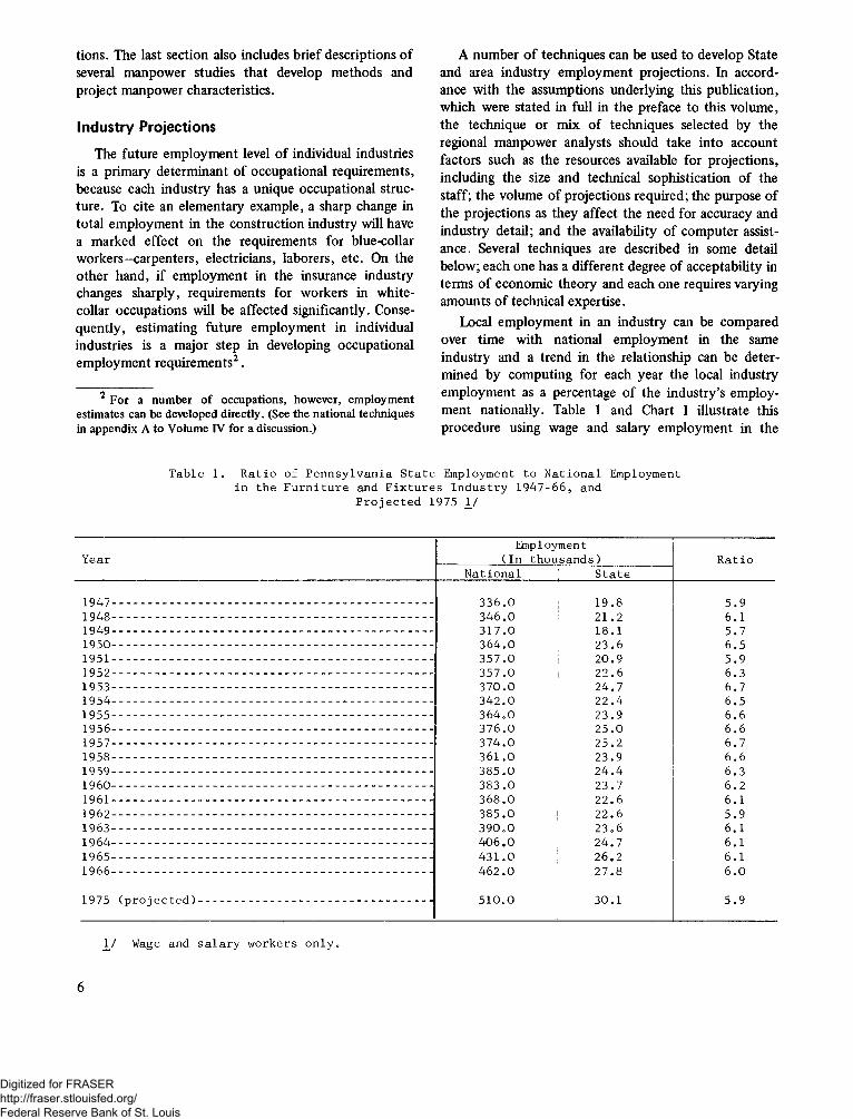
Local employment in an industry can be compared over time with national employment in the same industry and a trend in the relationship can be determined by computing for each year the local industry employment as a percentage of the industry’s employment nationally. Table 1 and Chart 1 illustrate this procedure using wage and salary employment in the
T a b l e 1 . R a t i o o f P e n n s y l v a n i a S t a t e E m p l o y m e n t t o N a t i o n a l E m pl o ym en t i n t h e F u r n i t u r e and F i x t u r e s I n d u s t r y 1 9 4 7 - 6 6 , and
P r o j e c t e d 1 9 7 5 1 /
Y e a rE m p l o y m e n t
( I n t h o u s a n d s ) R a t i oN a t i o n a l | S t a t e
1 9 4 7 ---------------------------------------------------------------------------------------------- 3 3 6 . 0 S 1 9 . 8 5 . 91 9 4 8 ---------------------------------------------------------------------------------------------- 3 4 6 . 0 ’ 2 1 . 2 6 .11 9 4 9 ------- ---------- ---------------------------------------------------------------------------- 3 1 7 oO 1 8 . 1 5 . 71 9 5 0 ----------------------------------------------------------------------------------- ---------- 3 6 4 . 0 2 3 . 6 6 . 51 9 5 1 ---------------------------------------------------------------------------------------------- 3 5 7 . 0 1 2 0 . 9 5 . 91 9 5 2 - --------- ---------------------------------------------------------------------------------- 3 5 7 . 0 i 2 2 . 6 6 . 31 9 5 3 ---------------------------------------------------------------------------------------------- 3 7 0 . 0 2 4 . 7 6 . 71 9 5 4 - - ------------------------------------------------------------------------------------------ 3 4 2 . 0 2 2 . 4 6 . 51 9 5 5 ----------------------------------------------- -------------- ------------------------------- 3 6 4 . 0 2 3 . 9 6 .61 9 5 6 --------------------------------------------------- ------------------------------------------ 3 7 6 . 0 2 5 . 0 6 .61 9 5 7 ---------------------------------------------------------------------------------------------- 3 7 4 . 0 2 5 . 2 6 . 71 9 5 8 ---------------------------------------------------------------------------------------------- 3 6 1 . 0 2 3 . 9 6 .61 9 5 9 ---------------------------------------------------------------------------------------------- 3 8 5 . 0 2 4 . 4 6 . 3I 9 6 0 -------------------------- -------------------------------------------- -------------- -------- 3 8 3 . 0 2 3 . 7 6 o 21 9 6 1 ----------------------------------------------------------------------------------- ---------- 3 6 8 . 0 2 2 .6 6 .11 9 6 2 ---------------------------------------------------------------------------------------------- 3 8 5 . 0 | 2 2 . 6 5 . 91 9 6 3 ..................................................................................................... ........... .............. 3 9 0 . 0 23 o 6 6 .11 9 6 4 --------- ------------------------------------------------------------------------------------ 4 0 6 . 0 2 4 . 7 6 .11 9 6 5 ------------------------------------------------------------------ -------------- ------------ 4 3 1 . 0 ; 2 6 . 2 6 .11 9 6 6 ---------------------------------------------------------------------------------------------- 4 6 2 . 0 2 7 . 8 6 .0
1 9 7 5 ( p r o j e c t e d ) -------------------------------------------------------------------- 5 1 0 . 0 3 0 . 1 5 . 9
1 / Wage and s a l a r y w o r k e r s o n l y 0
6
Digitized for FRASER http://fraser.stlouisfed.org/ Federal Reserve Bank of St. Louis
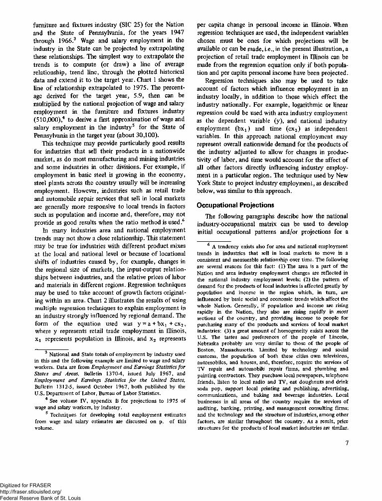
furniture and fixtures industry (SIC 25) for the Nation and the State of Pennsylvania, for the years 1947 through 1966.3 Wage and salary employment in the industry in the State can be projected by extrapolating these relationships. The simplest way to extrapolate the trends is to compute (or draw) a line of average relationship, trend line, through the plotted historical data and extend it to the target year. Chart 1 shows the line of relationship extrapolated to 1975. The percentage derived for the target year, 5.9, then can be multiplied by the national projection of wage and salary employment in the furniture and fixtures industry (510,000),4 to derive a first approximation of wage and salary employment in the industry5 for the State of Pennsylvania in the target year (about 30,100).
This technique may provide particularly good results for industries that sell their products in a nationwide market, as do most manufacturing and mining industries and some industries in other divisions. For example, if employment in basic steel is growing in the economy, steel plants across the country usually will be increasing employment. However, industries such as retail trade and automobile repair services that sell in local markets are generally more responsive to local trends in factors such as population and income and, therefore, may not provide as good results when the ratio method is used.6
In many industries area and national employment trends may not show a close relationship. This statement may be true for industries with different product mixes at the local and national level or because of locational shifts of industries caused by, for example, changes in the regional size of markets, the input-output relationships between industries, and the relative prices of labor and materials in different regions. Regression techniques may be used to take account of growth factors originating within an area. Chart 2 illustrates the results of using multiple regression techniques to explain employment in an industry strongly influenced by regional demand. The form of the equation used was y = a + bx1 +cx2, where y represents retail trade employment in Illinois, Xi represents population in Illinois, and x2 represents
3 National and State totals of employment by industry used in this and the following example are limited to wage and salary workers. Data are from E m ploym en t and Earnings Statistics for States and Areas, Bulletin 1370-4, issued July 1967, and E m ploym en t and Earnings Statistics fo r the United States, Bulletin 1312-5, issued October 1967, both published by the U.S. Department of Labor, Bureau of Labor Statistics.
4 See volume IV, appendix B for projections to 1975 of wage and salary workers, by industry.
5 Techniques for developing total employment estimates from wage and salary estimates are discussed on p. of this volume.
per capita change in personal income in Illinois. When regression techniques are used, the independent variables chosen must be ones for which projections will be available or can be made,i.e.,in the present illustration, a projection of retail trade employment in Illinois can be made from the regression equation only if both population and per capita personal income have been projected.
Regression techniques also may be used to take account of factors which influence employment in an industry locally, in addition to those which effect the industry nationally. For example, logarithmic or linear regression could be used with area industry employment as the dependent variable (y), and national industry employment (bxx) and time (cx2) as independent variables. In this approach national employment may represent overall nationwide demand for the products of the industry adjusted to allow for changes in productivity of labor, and time would account for the affect of all other factors directly influencing industry employment in a particular region. The technique used by New York State to project industry employment, as described below, was similar to this approach.Occupational Projections
The following paragraphs describe how the national industry-occupational matrix can be used to develop initial occupational patterns and/or projections for a
6 A tendency exists also for area and national employment trends in industries that sell in local markets to move in a consistent and measurable relationship over time. The following are several reasons for this fact: (1) The area is a part of the Nation and area industry employment changes are reflected in the national industry employment levels; (2) the pattern of demand for the products of local industries is affected greatly by population and income in the region which, in turn, are influenced by basic social and economic trends which affect the whole Nation. Generally, if population and income are rising rapidly in the Nation, they also are rising rapidly in m ost sections of the country, and providing income to people for purchasing many of the products and services of local market industries; (3) a great amount of homogeneity exists across the U.S. The tastes and preferences of the people of Lincoln, Nebraska probably are very similar to those of the people of Boston, Massachusetts. Limited by technology and social customs, the population of both these cities own televisions, automobiles, and houses, and, therefore, require the services of TV repair and automobile repair firms, and plumbing and painting contractors. They purchase local newspapers, telephone friends, listen to local radio and TV, eat doughnuts and drink soda pop, support local printing and publishing, advertising, communications, and baking and beverage industries. Local businesses in all areas of the country require the services of auditing, banking, printing, and management consulting firms; and the technology and the structure of industries, among other factors, are similar throughout the country. As a result, price structures for the products of local market industries are similar.
7
Digitized for FRASER http://fraser.stlouisfed.org/ Federal Reserve Bank of St. Louis
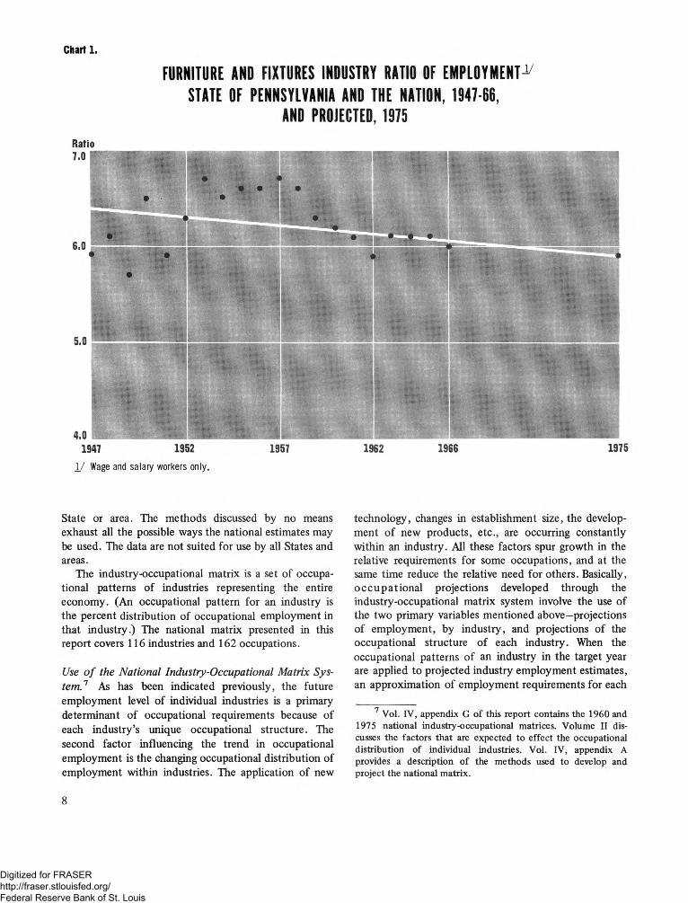
Chart 1.FURNITURE AND FIXTURES INDUSTRY RATIO OF EMPLOYMENT
STATE OF PENNSYLVANIA AND THE NATION, 1947-66,AND PROJECTED, 1975
Ratio
1947 1952 1957 1962 1966 1975
1/ Wage and salary workers only.
State or area. The methods discussed by no means exhaust all the possible ways the national estimates may be used. The data are not suited for use by all States and areas.
The industry-occupational matrix is a set of occupational patterns of industries representing the entire economy. (An occupational pattern for an industry is the percent distribution of occupational employment in that industry.) The national matrix presented in this report covers 116 industries and 162 occupations.Use o f the N ation a l Indu stry-O ccu pational M atrix S y ste m .1 As has been indicated previously, the future employment level of individual industries is a primary determinant of occupational requirements because of each industry’s unique occupational structure. The second factor influencing the trend in occupational employment is the changing occupational distribution of employment within industries. The application of new
technology, changes in establishment size, the development of new products, etc., are occurring constantly within an industry. All these factors spur growth in the relative requirements for some occupations, and at the same time reduce the relative need for others. Basically, occupational projections developed through the industry-occupational matrix system involve the use of the two primary variables mentioned above—projections of employment, by industry, and projections of the occupational structure of each industry. When the occupational patterns of an industry in the target year are applied to projected industry employment estimates, an approximation of employment requirements for each
7 Vol. IV, appendix G of this report contains the 1960 and 1975 national industry-occupational matrices. Volume II discusses the factors that are expected to effect the occupational distribution of individual industries. Vol. IV, appendix A provides a description of the methods used to develop and project the national matrix.
8
Digitized for FRASER http://fraser.stlouisfed.org/ Federal Reserve Bank of St. Louis
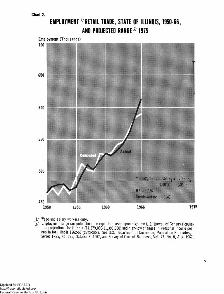
Chart 2.
EMPLOYMENT-RETAIL TRADE, STATE OF ILLINOIS, 1050-06, AND PROIECTED RANGE- 1 9 7 5
Employment (Thousands)
1950 1955 1960 1966 1975J / Wage and salary workers only.
2/ Employment range computed from the equation based upon high-low U.S. Bureau of Census Population projections for Illinois (1 1 ,8 7 9 ,0 0 0 -1 1 ,3 9 5 ,0 0 0 ) and high-low changes in Personal Income per capita for Illinois 1 9 6 2 -6 6 ($2 4 2 -$8 9 ). See U.S. Department of Commerce, Population Estimates, Series P-2 5 , No. 3 7 5 , October 3 , 1 9 6 7 , and Survey of Current Business, Vol. 4 7 , No. 8, Aug. 1 9 6 7 .
9
Digitized for FRASER http://fraser.stlouisfed.org/ Federal Reserve Bank of St. Louis
of the occupations in the matrix is derived. By following this procedure for each industry and summing the results, estimates of total requirements for each occupation can be obtained.
The development of State and area occupational projections through the use of the national industry- occupational matrices is possible through a variety of methods. The following discussion is limited to two techniques which appear to offer promise.8 The first is a relatively simple system that is dependent upon both the base period national matrix (1960) and the projected national matrix (1975). The second technique is more complex; it requires the development of an area base period (1960) matrix. An area matrix then may be projected to the target year by applying the national trends in the occupational structure of each industry to the occupational structure of corresponding industries in the area base period matrix.
The first step of any method in which national matrices are used is to make area industry employment estimates consistent with the total employment concept on which the national industry-occupational matrix is based. Private wage and salary employment, by industry, must be modified to include the other three classes of workers, i.e., self-employed, unpaid family workers, and government9 workers. Additional refinements also should be made to the wage and salary employment estimates. The first involves an adjustment to a one- person one-job concept, which can be made by deducting the secondary jobs of multiple job holders. The second refinement accounts for persons employed but not at work (unpaid absences).10
The table presented in volume IV, appendix D illustrates the proportion, nationally, of private wage and salary workers to total employment for each industry. Private wage and salary workers make up the largest share of workers in most industries. As is shown, the importance of the “other workers” varies widely
Q A third method, somewhat different than either of these, was followed by New York State and is described later in this chapter.
9 Government workers involved in activities unique to government are classified in the public administration industry. Government workers in agencies engaged in activities also carried on by private enterprises, such as education and medical services, construction, transportation, and manufacturing, are classified in their appropriate industry category, regardless of whether they are paid from private or public funds.
10 For information on multiple job holders and unpaid absences, see the H andbook o f Labor Statistics 1967, U.S. Department of Labor, Bureau of Labor Statistics. For sale by the U.S. Government Printing Office, Washington, D.C., 20402, Price $2.
among the industries. Self-employed and unpaid family workers are especially important in industries such as agriculture; several service industries, including legal, engineering, and medical services; retail trade; and construction. Government workers make up a significant part of the work force in industries such as educational services, local public utilities, hospitals, shipbuilding, and construction.
Two basic methods can be used by the area manpower specialist to estimate the employment of these three classes of workers. The simplest technique would be to adopt the national relationships as shown in volume IV, appendix D for both 1960 and 1975. This technique might prove satisfactory for industries in which the workers other than wage and salary workers are relatively unimportant, but in others, particularly those where large numbers of government workers are concentrated, local analysts may want to develop their own estimates through the use of other data.11
Once area industry employment estimates on the total employment concept have been developed for both 1960 and 1975, first approximations of projected area occupational employment requirements may then be derived through one of the following methods.A rea P rojection M eth o d A . 12 This technique uses the national base period and projected matrices, and does not require a special area matrix. In general, estimates of area occupational requirements are made by applying 1960 and 1975 national industry-occupational patterns to their appropriate area industry employment estimates for each year; summing the resulting occupational employment to area totals; computing the 1960 to 1975
11 Industry employment is reported separately for each class of worker in 1950 U.S. Census of Population, Vol. II, Characteristics o f the Population, Table No. 83, and 1960 U.S. Census o f Population, Vol. I, Characteristics o f the Population, Table No. 129, U.S. Department of Commerce, U.S. Bureau of the Census. These data are available for all States and for Standard Metropolitan Statistical Areas that have a population of over 250,000. The Population Census data should provide a basis for estimating employment levels for self-employed, unpaid family, and government workers, and for determining the trend in employment of these workers by industry. Additional information on employment of government workers also is available from the Census o f Government, 1966, Vol. I ll, Compendium o f Public E m ploym ent, and the annual reports on State D istribution o f Public E m ploym ent, published by the Bureau of the Census. Information on self-employed workers in selected industries is available from the 1963 and earlier editions of the Census of Busiijess and the Census of Manufacturers, also published by the Bureau of the Census.12 See footnote 17 for a mathematical expression of Method A.
1 0
Digitized for FRASER http://fraser.stlouisfed.org/ Federal Reserve Bank of St. Louis
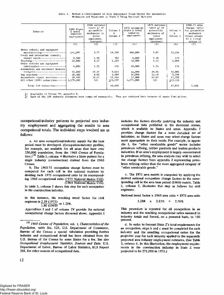
change factors (percent change) for each occupation; and applying the change factors to separately estimated 1960 area occupational employment totals. The individual steps involved are:
applying the change factor to the base period area em ploym ent determ ined in step “ c ” . By applying the change factor in table 2, the estim ated 1975 em ploym ent for autom obile m echanics and repairmen in State Z is calculated to be 59 ,480:
a. The 1960 national industry-occupational patterns are applied to their respective 1960 area industry em ploym ent estim ates. The resulting occupational em ploym ent is then sum med to area totals. This same procedure is fo llow ed using the 1975 national industry-occupational patterns and projected area industry em ploym ent estimates. In table 2 , this step is illustrated in colum n 3 (19 6 0 ) and colum n 6 (19 7 5 ). In this exam ple, the tw o aggregates were 4 2 ,6 6 0 for 1960 and 5 7 ,9 21 for 1975 .
b . The 1960-75 change factor for the occupations then m ust be com puted b y dividing the 1975 em ploym ent aggregate by the 1960 em ploym ent aggregate developed in step “a” . In table 2 , the resulting change factor for autom obile m echanics and repairmen was 57 ,9 21 or 1 .358 .4 2 ,6 6 0
c. Base period (1 9 6 0 ) area em ploym ent estim ates m ust be made for each occupation for which projections are desired. The 1960 Census1 3 can supply the basic data needed for these estim ates . 1 4 (Other data sources should be investigated and utilized, i f available . ) 1 5 For illustrative purposes, the base period (1 9 6 0 ) em ploym ent o f autom obile m echanics and repairmen in State Z was reported 1 6 to be 4 3 ,8 0 0 workers. This num ber is som ew hat higher than the 1960 em ploym ent com puted in step “b ” . Such differences should be expected , since the patterns used in step “b ” are national averages. The differences in the estim ates developed in steps b . and c. p oin t ou t that in one or more industries a higher proportion o f autom obile m echanics and repairmen are em ployed in State Z than the national average.
d. The initial 1975 em ploym ent estim ate o f autom obile m echanics and repairmen then m ay be com puted by
1 3 1 9 6 0 Census o f P opulation , V ol. I, Characteristics o f the Population, Parts 1-50, tables 7 4 , 84 , and 12 1 , U .S. Department o f C om m erce, Bureau o f the Census.
1 4 The U .S. Census o f Population is the major source o f detailed occupational em ploym ent statistics. Users o f these data should be aware o f their lim itations, such as general undercount, possible response errors, classification problem s, etc. For a more thorough evaluation o f the Census occupational em ploym ent data see O ccupational E m p lo y m en t S ta tistics, Sources an d Data, BLS Report 30 5 , or Evaluation an d R esearch Program o f the U.S. Census o f Population an d H ousing 1960: The E m p lo yer R e co rd Check, Series E R 60, N o. 6 . U .S . Departm ent o f Com m erce, Bureau o f the Census.
1 5 See, for exam ple, O ccupational E m p lo y m en t S tatistics, Sources an d D ata , U .S. Departm ent o f Labor, Bureau o f Labor Statistics, BLS Report 305.
1 6 The reported 4 3 ,8 0 0 workers in 1960 may have com e from such sources as the Census o f Population 1 9 60 or an Area Skill Survey for that year.
Occupational Trend Factor (1 .3 5 8 ) x Base Period O ccupation Em ploym ent (4 3 ,8 0 0 )
1 .3 5 8 x 4 3 ,8 0 0
1975 Em ploym ent o f A utom obile Mechanics and Repairmen in State Z
= 5 9 ,4 8 0The above procedure must be repeated for each
occupation for which projections are desired. When this procedure is used, local projections are possible for each occupation and occupation group included in the national matrices.A rea P rojection M eth o d B } 1 Method B integrates national industry-occupational structure trends with a specially developed area base period matrix. In order to use method B, an area base period industry-occupational matrix must be developed independently. Then, an area target year (1975) matrix is computed by applying the changes, 1960-75, projected for the industry- occupational structures at the national level to the corresponding industries in the area base period, 1960, matrix. Initial 1975 area occupational employment estimates then can be made by applying the 1975 area
1 7 A m athem atical form ula for m ethods A and B follow s:
M ethod A n2 fjj(75) I 4 (75 )
Lj(75) = i= l------------------------------------------------L j(60)
n2 fij(60 ) Lj(60)i= l
M ethod B nLj(75) = 2 L if(7 5 ) . L i(75)
i= lwhere Lij*(75) = fy (7 5 )
fij(60 ) . Ljj*(6 0 )
Ly (year) is local em ploym ent by industry i and occupation j in the given year.
Lj (year) is total local em ploym ent in industry i in the given year.
fjj (year) is national fraction o f occupation j in industry i in the given year.
Li* (year) is local fraction o f occupation j in industry i in given year.
Lj (year) is total local em ploym ent in occupation j.
11
Digitized for FRASER http://fraser.stlouisfed.org/ Federal Reserve Bank of St. Louis
T a b le 2. Method A --D eve lopm en t o f A rea Employment Trend F a c to r f o r A u tom ob ile M echan ics and Repairm en in S ta te Z U sing N a t io n a l M a tr ic e s
In d u s try1960 S ta te Z t o t a l in d u s try
employment
1960 n a t io n a l r a t i o JV o f a u tom ob ile
m echanics to t o t a l
employment(p e r c e n t )
Column 1 X
Column 2
1975 e s t im a ted S ta te Z t o t a l
in d u s try employment
1975 n a t io n a l r a t i o IV o f au tom ob ile
m echan ics o f t o t a l
employment(p e r c e n t )
Column 4 X
Column 5
1960-75 a rea change fa c t o r
f o r a u tom ob ile m echanics
( t o t a l column 6) f ( t o t a l
c o 1umn 3 )(1 ) (2 ) (3 ) (4 ) ( 5 ) (6 ) ( 7 )
M otor v e h ic l e and equipm entm a n u fa c tu r in g ------------------------------- 377,200 3.77 14,220 408,000 3 .07 12,526
L o c a l and in te ru rb a n t r a n s i t ,e x c e p t t a x i s --------------------------------- 8 ,500 6 .96 592 8,000 5.29 423
T ru c k in g -------------------------------------------- 35,900 3 .37 1,210 45,000 4 .15 1,868M otor v e h ic l e and equ ipm ent
(w h o le s a le ) ----------------------------------- 6,000 1.72 103 10,000 1.74 174A u tom ob ile and a c c e s s o ry d e a le r s
( r e t a i l ) ---------------------------------------- 35,200 27.31 9,613 54,000 29.64 16,006Gas s t a t i o n s ------------------------ ------------ 28,300 8 .83 2,499 44,000 12.49 5,496A u tom ob ile r e p a ir s e r v i c e s ----------- 20,400 55.47 11,316 37,000 47.85 17,705A l l o th e r (1 0 9 ) in d u s t r ie s ----------- 3 ,179 ,500 (2 ) 2/3,107 4 ,174 ,000 (2 ) 2/3,723
T o ta l 116 in d u s t r ie s ------------- 42,660 57,921 1.358
IV A v a i la b le in Volume IV , appen d ix G.2/ Each o f the 109 in d u s try e s t im a te s w ere computed s e p a r a t e ly . They a re combined h e re because o f space l im i t a t i o n s .
occupational-industry patterns to projected area industry employment and aggregating the results to area occupational totals. The individual steps involved are as follows:
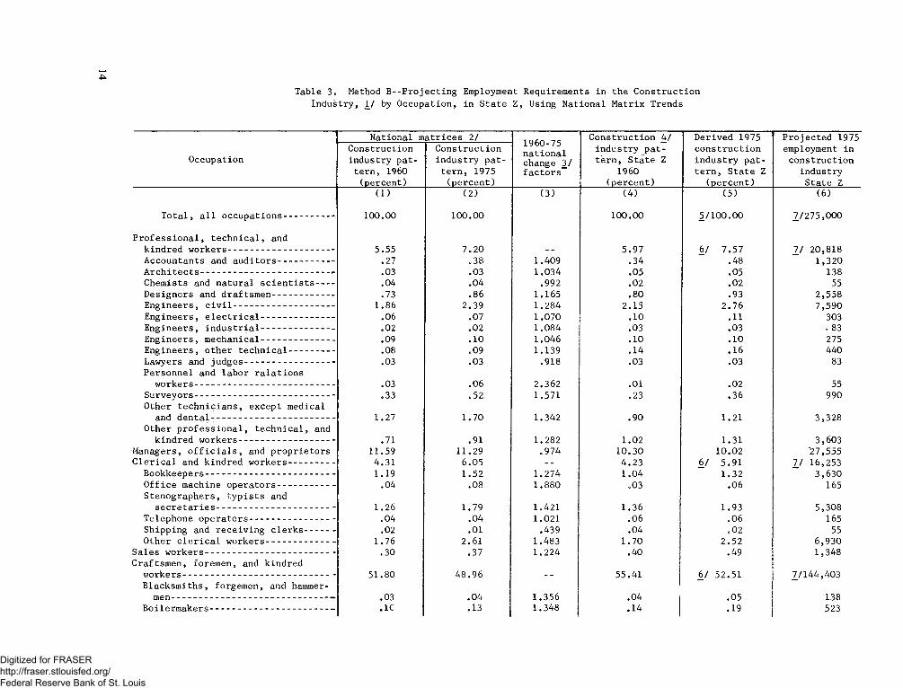
a. An area occupational-industry matrix for the base period m ust be developed. (Occupation-industry profiles, for exam ple, are available for all areas that have over2 5 0 ,0 0 0 population , from the 1960 Census o f Population . ) 1 8 Table 3, colum n 4 illustrates a State pattern for a single industry (construction) derived from the 1960 Census.
b. The 1960-75 occupation change factors m ust be com puted for each cell in the national m atrices by dividing each 1975 occupational ratio b y its corresponding 1960 occupational ratio (1975 National Matrix Cell).
(1 9 6 0 National Matrix Cell).In table 3, colum n 3 shows this step for each occupation in the construction industry.
In this instance, the resulting trend factor for civil engineers is 2 .39 (1 9 7 5 ) , . . .
1.86 (I 9 6 0 ) ’ 0 1 1 -284‘A ppendixes I and J o f volum e IV provide the national occupational change factors discussed above. A ppendix I
18 1 9 6 0 Census o f P opulation , vol. I, C haracteristics o f the P opu la tio n . table N o. 125 , U .S. Departm ent o f Com m erce, Bureau o f the Census a special tabulation providing further industry and occupational detail has been obtained from the U .S. Bureau o f the Census by some States for a fee . See also O ccupational E m p lo y m en t S ta tistics, Sources an d D ata, U .S. Departm ent o f Labor, Bureau o f Labor Statistics, BLS Report 30 5 , for other sources o f occupational data.
includes the factors directly m atching the industry and occupational data published in the decennial census, w hich is available to States and areas. A ppendix J provides change factors for a more d e ta ile d set o f industries, so States and areas m ay select change factors m ost appropriate to their needs. For exam ple, in appendix I, the “ other nondurable good s” sector includes petroleum refining, rubber products and leather products industries. I f an area’s em ploym ent is largely concentrated in petroleum refining, the area analysts may wish to select the change factors from appendix J representing petroleum refining rather than the more aggregated category o f “other nondurable good s.”
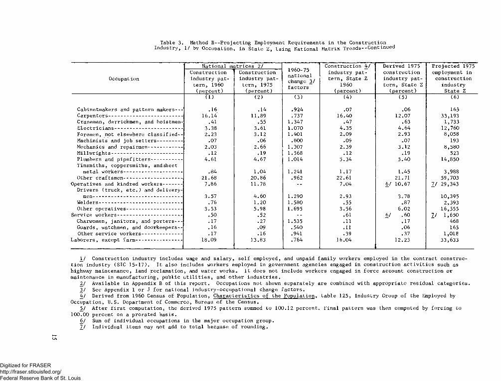
c. The 1975 area matrix is com puted b y applying the derived national occupation change factors to the corresponding cell in the area base period (1 9 6 0 ) m atrix. Table 3, colum n 5 , illustrates this step as fo llow s for civil engineers:N ational trend factor x 1960 area ratio = 1975 area ratio
1 .284 x 2.15% = 2.76%
This procedure is repeated for all occupations in an industry and the resulting occupational ratios sum med to industry totals and forced, on a prorated basis, to 1 0 0
percent.d. In order to forecast State Z’s total requirem ents for
an occupation, steps b and c m ust be com pleted for each industry and the resulting occupational ratios for the projected year for each industry applied to the separately projected area industry em ploym ent estim ates. (See Table 3, colum n 6 . In this illustration, the em ploym ent requirem ents in the construction industry in State Z were projected to be 2 7 5 ,0 0 0 in 1 9 75 .)
1 2
Digitized for FRASER http://fraser.stlouisfed.org/ Federal Reserve Bank of St. Louis
The resulting occupational estim ate for each industry canthen be aggregated to obtain the area’s total em ploym entrequirements for the occupation in the target year.
Occupational projections developed through the use of relatively mechanical systems such as those discussed in the preceding paragraphs, should be viewed only as first approximations. They do, however, provide the local manpower analyst a base upon which to begin his evaluation. Method A seems to offer the best balance between the systems input requirements and the quality and quantity of projections produced. Its relative simplicity and adaptability to smaller areas makes it especially attractive. Method B is a more complex approach. The development of the special area matrix required by this technique could prove to be a difficult and resource consuming task. Furthermore, the projections might prove less desirable, if data limitations forced the creation of an area matrix with considerably less industry detail than that available at the national level. The occupational structures of detailed industries are sometimes significantly different than that of the industry group of which they are a part. On the other hand, an area matrix with relatively detailed industry base, such as that which may be obtained from a special Census tabulation, would have many advantages. For example, it would provide the area analyst a tool to develop current occupational employment estimates by utilizing the base period occupational structure, on the assumption that occupational patterns do not change significantly in the short run, or by adjusting the base period structure on the basis of new data.
The use of the national matrices also offers the prospect of preparing a range of occupational projections based on differing assumptions of an area’s future economic conditions by developing alternative projections of industry employment or by modifying the changes expected in the occupational structure of an area’s key industries. Such flexibility may prove especially valuable in States and areas where the industrial structure is changing rapidly and where future levels of industry employment depend greatly on factors such as defense expenditures, which are difficult to predict.
The growth in employment requirements for each occupation determined through the methods discussed above or similar methods are but a first step in estimating the overall occupational requirements in the projected period. To the growth estimates must be added replacement needs expected as a result of deaths, retirements, and transfers of experienced workers to other occupations. Several methods for estimating such openings are discussed in the following chapter.
T est o f M eth o d A . A test of occupational projection method A was made to provide a basis for evaluating its accuracy. A less complex method (A1) also was tested to determine whether more accurate projections were attained by “localization” of the national matrix (steps c and d, page ) in method A. Test method A1 was based on the assumption that an area’s industry-occupational p a ttern s , in addition to its trends (method A), are the same as national industry-occupational patterns in the base and projected years.
The test of the technique was limited, because it was performed for one State and focused on the accuracy of method A only. It assumed that industry employment projections for Ohio made in 1950 for 1960 were perfect. It further assumed that projections of national industry-occupational patterns made in 1950 for 1960 also were perfect. In reality, error would be involved in each of these steps, in addition to the error associated with the collection of the basic data.
Data on 40 occupations for the nation and the State of Ohio in 1950 and 1960 were used in the test. National industry-occupational patterns for 1950 and I96019 were applied to detailed industry employment totals for Ohio in 1950 and I96020, respectively. Preliminary 1950 and 1960 estimates of occupational employment in Ohio were derived by summing employment in each of the 40 occupations across all industries. Final projections (method A) were made by deriving a coefficient of occupational change for each occupation between 1950 and 1960, and applying it to the respective occupational totals for 1950, as shown in the Census of Population, 1960, for Ohio. For method A1, the preliminary projections based solely on national industry-occupational patterns and trends were considered the final projections.
Table 4 presents the results of the test of projection method A, shown as a percent of actual occupational employment in Ohio in 1960. Of the 31 detailed occupations in the test of method A, 18 were projected between 105 and 95 percent of actual employment in 1960, and 27 between 110 and 90 percent. Differences in industry product mix in Ohio and the nation were important determinants of those projections that were significantly in error. For example, the projection of
1 9 Derived from data in the U.S. Census o f P opulation: 1960 , O ccupation by In du stry , Final Report PC(92)-7C. U .S. Departm ent o f C om m erce, Bureau o f the Census 1963 .
20 U.S. Census o f P opulation: 19 60 , D e ta iled Characteristics, O hio, Final R e p o r t P C (1)-37D . U .S . Departm ent o f C om m erce, Bureau o f the Census.
13
Digitized for FRASER http://fraser.stlouisfed.org/ Federal Reserve Bank of St. Louis
T a b le 3 . M ethod B - - P r o j e c t i n g E m ploym ent R e q u ir e m e n ts in t h e C o n s t r u c t io n I n d u s t r y , 1 / by O c c u p a t io n , in S t a t e Z , U s in g N a t io n a l M a tr ix T ren d s
O c c u p a t io nN a t io n a l m a t r i c e s 2 / C o n s t r u c t io n 4 /
i n d u s t r y p a t t e r n , S t a t e Z
19 6 0( p e r c e n t )
D e r iv e d 1 9 75 1 c o n s t r u c t i o n i n d u s t r y p a t t e r n , S t a t e Z
( p e r c e n t )
P r o j e c t e d 1975 em p loym en t in
c o n s t r u c t i o n in d u s t r y
S t a t e Z
C o n s t r u c t io n in d u s t r y p a t
t e r n , 1960 ( p e r c e n t )
C o n s t r u c t io n i n d u s t r y p a t
t e r n , 1975 ( p e r c e n t )
1 9 6 0 -7 5 n a t i o n a l c h a n g e 3 / f a c t o r s
( 1 ) ( 2 ) ( 3 ) ( 4 ) ( 5 ) (6 )
T o t a l , a l l o c c u p a t i o n s ---------------- - 1 0 0 .0 0 1 0 0 .0 0 1 0 0 .0 0 5 / 1 0 0 .0 0 7 / 2 7 5 ,0 0 0
P r o f e s s i o n a l , t e c h n i c a l , andk in d r e d w o r k e r s -------------------------------------- 5 .5 5 7 .2 0 5 .9 7 6 / 7 .5 7 7 / 2 0 ,8 1 8A c c o u n ta n ts and a u d i t o r s -------------------- .2 7 .3 8 1 .4 0 9 .3 4 .4 8 1 ,3 2 0A r c h i t e c t s ...... .................. - .................................. ■- .0 3 .0 3 1 .0 3 4 .0 5 .0 5 138C h e m is ts and n a t u r a l s c i e n t i s t s ------ .0 4 .0 4 .9 9 2 .0 2 .0 2 55D e s ig n e r s and d r a f t s m e n ---------------------- .7 3 .8 6 1 .1 6 5 .8 0 .9 3 2 ,5 5 8E n g in e e r s , c i v i l ------------------------------------ 1 .8 6 2 .3 9 1 .2 8 4 2 .1 5 2 .7 6 7 ,5 9 0E n g in e e r s , e l e c t r i c a l -------------------------- .0 6 .0 7 1 .0 7 0 .1 0 .1 1 303E n g in e e r s , i n d u s t r i a l - ................................. .0 2 .0 2 1 .0 8 4 .0 3 .0 3 . 83E n g in e e r s , m e c h a n ic a l -------------------------- .0 9 .1 0 1 .0 4 6 .1 0 .1 0 275E n g in e e r s , o t h e r t e c h n i c a l ....................- .0 8 .0 9 1 .1 3 9 .1 4 .1 6 44 0L a w yers and j u d g e s --------------------------------- .0 3 .0 3 .9 1 8 .0 3 .0 3 83P e r s o n n e l and la b o r r a l a t i o n s
w o r k e r s ---------------------------------------------- - - .0 3 .0 6 2 .3 6 2 .0 1 .0 2 55S u r v e y o r s ------------------------------------------------ -- .3 3 .5 2 1 .5 7 1 .2 3 .3 6 99 0O th e r t e c h n i c i a n s , e x c e p t m e d ic a l
and d e n t a l - ---------------------------------------- - 1 .2 7 1 .7 0 1 .3 4 2 .9 0 1 .2 1 3 ,3 2 8O th e r p r o f e s s i o n a l , t e c h n i c a l , and
k in d r e d w o r k e r s -------------------------------- -- .7 1 .9 1 1 .2 8 2 1 .0 2 1 .3 1 3 ,6 0 3M a n a g er s , o f f i c i a l s , and p r o p r ie t o r s 1 1 .5 9 1 1 .2 9 .9 7 4 1 0 .3 0 1 0 .0 2 '2 7 ,5 5 5C l e r i c a l and k in d r e d w o r k e r s ................... 4 .3 1 6 .0 5 4 .2 3 6 / 5 .9 1 7 / 1 6 ,2 5 3
B o o k k e e p e r s ---------------------------------------- ------ 1 .1 9 1 .5 2 1 .2 7 4 1 .0 4 1 .3 2 3 ,6 3 0O f f i c e m a ch in e o p e r a t o r s --------------------- .0 4 .0 8 1 .8 8 0 .0 3 .0 6 165S t e n o g r a p h e r s , t y p i s t s and
s e c r e t a r i e s ---------------------------------------- -- 1 .2 6 1 .7 9 1 .4 2 1 1 .3 6 1 .9 3 5 ,3 0 8T e le p h o n e o p e r a t o r s ------------------------------- .0 4 .0 4 1 .0 2 1 .0 6 .0 6 165S h ip p in g and r e c e i v i n g c l e r k s -------- -- .0 2 .0 1 .4 3 9 .0 4 .0 2 55O th e r c l e r i c a l w o r k e r s ------------------------- 1 .7 6 2 .6 1 1 .4 8 3 1 .7 0 2 .5 2 6 ,9 3 0
S a l e s w o r k e r s -------------------------------------------- -- .3 0 .3 7 1 .2 2 4 .4 0 .4 9 1 ,3 4 8C r a f ts m e n , fo r e m e n , and k in d r e d
w o r k e r s ------------------------------------------------------- 5 1 .8 0 4 8 .9 6 5 5 .4 1 6 / 5 2 .5 1 7 /1 4 4 ,4 0 3B l a c k s m i t h s , fo r g e m e n , and hammer-
m en-------------------------------------------------------- — .0 3 .0 4 1 .3 5 6 .0 4 .0 5 138B o i l e r m a k e r s --------------------------------------------- .1C .1 3 1 .3 4 8 .1 4 .1 9 523
Digitized for FRASER http://fraser.stlouisfed.org/ Federal Reserve Bank of St. Louis
T a b le 3 . M ethod B - - P r o j e c t i n g Em ploym ent R e q u ir e m e n ts i n t h e C o n s t r u c t io n I n d u s t r y , 1 / by O c c u p a t io n , in S t a t e Z , U s in g N a t io n a l M a tr ix T r e n d s - -C o n t in u e d
N a t io n a l m a t r i c e s 2 / 1 9 6 0 -7 5 n a t i o n a l c h a n g e 3 / f a c t o r s
C o n s t r u c t io n 4 / ’ D e r iv e d 1975 P r o j e c t e d 1975
O c c u p a t io nC o n s t r u c t io n in d u s t r y p a t - -
t e r n , 19 6 0 ( p e r c e n t )
C o n s t r u c t io n i n d u s t r y p a t
t e r n , 1975 ( p e r c e n t )
in d u s t r y p a t t e r n , S t a t e Z
19 6 0( p e r c e n t )
c o n s t r u c t i o n i n d u s t r y p a t t e r n , S t a t e Z
( p e r c e n t )
em p loym en t in c o n s t r u c t i o n
i n d u s t r y S t a t e Z
( 1 ) ( 2 ) ( 3 ) ( 4 ) ( 5 ) ( 6 )C a b in e tm a k e r s and p a t t e r n m a k er s----- .1 6 .1 4 .9 2 4 .0 7 .0 6 165C a r p e n t e r s ------------------------------------------------ 1 6 .1 4 1 1 .8 9 .7 3 7 1 6 .4 0 1 2 .0 7 3 3 ,1 9 3C ran em en , d e r r ic k m e n , and h o is tm e n - .4 1 .5 5 1 .3 4 7 .4 7 .6 3 1 ,7 3 3E l e c t r i c i a n s .................................... ....................... 3 .3 8 3 .6 1 1 .0 7 0 4 .3 5 4 . 6 4 1 2 ,7 6 0F o rem en , n o t e ls e w h e r e c l a s s i f i e d - - 2 .2 3 3 .1 2 1 .4 0 1 2 .0 9 2 .9 3 8 ,0 5 8M a c h in i s t s and jo b s e t t e r s ......... ............. .0 7 .0 6 .8 0 0 .0 9 .0 7 193M e c h a n ic s and r e p a ir m e n ---------------------- 2 .0 3 2 .6 6 1 .3 0 7 2 .3 9 3 .1 2 8 ,5 8 0M i l l w r i g h t s .............................................................. .1 2 .1 9 1 .5 6 8 .1 2 .1 9 523P lu m b er s and p i p e f i t t e r s --------------------T i n s m i t h s , c o p p e r s m it h s , and s h e e t
4 .6 1 4 .6 7 1 .0 1 4 5 .3 4 5 . 4 0 1 4 ,8 5 0
m e ta l w o r k e r s ---------------------- --------------- .8 4 1 .0 4 1 .2 4 1 1 .1 7 1 .4 5 3 ,9 8 8O th e r c r a f t s m e n ................. .................................. 2 1 .6 8 2 0 .8 6 .9 6 2 2 2 .6 1 2 1 .7 1 5 9 ,7 0 3
O p e r a t iv e s and k in d r e d w o r k e r s ------------D r iv e r s ( t r u c k , e t c . ) and d e l i v e r y -
7 .8 6 1 1 .7 8 7 .0 4 6 / 1 0 .6 7 7 / 2 9 ,3 4 3m en-------------------------------------------- - ............... 3 .5 7 4 . 6 0 1 .2 9 0 2 .9 3 3 .7 8 1 0 ,3 9 5
W e ld e r s -------------------------------------------- --------- .7 6 1 .2 0 1 .5 8 0 .5 5 .8 7 2 ,3 9 3O th e r o p e r a t i v e s ------------------------------------ 3 .5 3 5 .9 8 1 .6 9 5 3 .5 6 6 .0 2 1 6 ,5 5 5
S e r v i c e w o r k e r s - ............- ------------- --------------- .5 0 .5 2 .6 1 6 / .6 0 7 / 1 ,6 5 0Charw om en, j a n i t o r s , and p o r t e r s - *- .1 7 .2 7 1 .5 3 5 .1 1 .1 7 468G u a r d s , w atch m en , and d o o r k e e p e r s - - .1 6 .0 9 .5 4 0 .1 1 .0 6 165O th er s e r v i c e w o r k e r s - - .............................. .1 7 .1 6 .9 4 1 .3 9 .3 7 1 ,0 1 8
L a b o r e r s , e x c e p t f a r m - .............. .................... - 1 8 .0 9 1 3 .8 3 .7 6 4 1 6 .0 4 1 2 .2 3 3 3 ,6 3 3
1 / C o n s t r u c t io n i n d u s t r y in c l u d e s wage and s a l a r y , s e l f e m p lo y e d , and u n p a id f a m i ly w o r k e r s e m p lo y e d in t h e c o n t r a c t c o n s t r u c t i o n i n d u s t r y (SIC 1 5 - 1 7 ) . I t a l s o in c l u d e s w o r k e r s em p lo y e d i n g o v e r n m e n t a g e n c ie s e n g a g e d in c o n s t r u c t i o n a c t i v i t i e s su c h a s h ig h w a y m a in t e n a n c e , la n d r e c la m a t io n , and w a te r w o r k s . I t d o e s n o t i n c l u d e w o r k e r s e n g a g e d in f o r c e a c c o u n t c o n s t r u c t i o n o r m a in te n a n c e in m a n u fa c tu r in g , p u b l i c u t i l i t i e s , and o t h e r i n d u s t r i e s .
2 / A v a i l a b l e in A p p en d ix B o f t h i s r e p o r t . O c c u p a t io n s n o t show n s e p a r a t e l y a r e com b in ed w i t h a p p r o p r i a t e r e s i d u a l c a t e g o r i e s .3 / S ee A p p e n d ix I o r J f o r n a t io n a l i n d u s t r y - o c c u p a t i o n a l c h a n g e f a c t o r s .4 / D e r iv e d from 19 60 C en su s o f P o p u l a t i o n , C h a r a c t e r i s t i c s o f th e P o p u l a t i o n , t a b l e 1 2 5 , I n d u s t r y Group o f t h e E m ployed by
O c c u p a t io n , U .S . D ep a rtm en t o f Com m erce, B u reau o f th e C e n s u s .5 / A f t e r f i r s t c o m p u ta t io n , th e d e r iv e d 19 75 p a t t e r n summed t o 1 0 0 .1 2 p e r c e n t . F in a l p a t t e r n w as th e n com p u ted by f o r c i n g to
1 0 0 .0 0 p e r c e n t on a p r o r a te d b a s i s .6 / Sum o f i n d i v i d u a l o c c u p a t io n s in th e m a jo r o c c u p a t io n g r o u p .7 / I n d i v id u a l i te m s may n o t add to t o t a l b e c a u s e o f r o u n d in g .
Digitized for FRASER http://fraser.stlouisfed.org/ Federal Reserve Bank of St. Louis
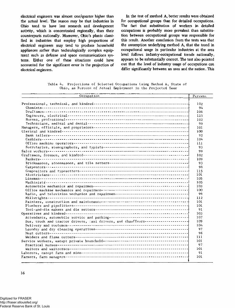
electrical engineers was almost one/quarter higher than the actual level. The reason may be that industries in Ohio tend to have less research and development activity, which is concentrated regionally, than their counterparts nationally. Moreover, Ohio’s plants classified in industries that employ high proportions of electrical engineers may tend to produce household appliances rather than technologically complex equipment such as defense and space communications systems. Either one of these situations could have accounted for the significant error in the projection of electrical engineers.
In the test of method A, better results were obtained for occupational groups than for detailed occupations. The fact that substitution of workers in detailed occupations is probably more prevalent than substitution between occupational groups was responsible for this result. Another conclusion from the tests was that the assumption underlying method A, that the trend in occupational usage in particular industries at the area level follows industry-occupational trends nationally, appears to be substantially correct. The test also pointed out that the level of industry usage of occupations can differ significantly between an area and the nation. This
T a b le 4 0 P r o j e c t i o n s o f S e l e c t e d O c c u p a t io n s U s in g M eth od A , S t a t e o f O h io , a s P e r c e n t o f A c t u a l E m p loym en t i n t h e P r o j e c t e d Y e a r
O c c u p a t io n P e r c e n t
P r o f e s s i o n a l , t e c h n i c a l , and k i n d r e d ------------------------------ ---------- ------------C h e m i s t s -------------------------------------------------------------------------------------------------------------D r a f t s m e n -----------------------------------------------------------------------------------------------------------E n g i n e e r s , e l e c t r i c a l ---------------------------------------------------------------------------------N u r s e s , p r o f e s s i o n a l -----------------------------------------------------------------------------------T e c h n i c i a n s , m e d i c a l an d d e n t a l ------------------------------------------------------------
M a n a g e r s , o f f i c i a l s , an d p r o p r i e t o r s ------------------------------------------------------C l e r i c a l an d k i n d r e d ----------------------------------------------------------------------------------------
B ank t e l l e r s ----------------------------------------------------------------------------------------------------C a s h i e r s -------------------------------------------------------------------------------------------------------------O f f i c e m a c h in e o p e r a t o r s ---------------------------------------------------------------------------S e c r e t a r i e s , s t e n o g r a p h e r s , an d t y p i s t s -------------------------------------------
S a l e s w o r k e r s ------------------------------------------------------------------------------------------------------C r a f t s m e n , f o r e m e n , an d k i n d r e d ----------------------------------------------------------------
B a n k e r s ---------------------------------------------------------------------------------------------------------------B r ic k m a s o n s , s t o n e m a s o n s , an d t i l e s e t t e r s -------------------------------------C a r p e n t e r s ---------------------------------------------------------------------------------------------------------C o m p o s i t o r s an d t y p e s e t t e r s --------------------------------------------------------------------E l e c t r i c i a n s ----------------------------------------------------------------------------------------------------L in e m e n ---------------------------------------------------------------------------------------------------------------M a c h i n i s t s --------------------------------------------------------------------------------------------------------A u t o m o b il e m e c h a n ic s and r e p a ir m e n ------------------------------------------------------O f f i c e m a c h in e m e c h a n ic s an d r e p a i r m e n ---------------------------------------------R a d io , an d t e l e v i s i o n m e c h a n ic s and r e p a ir m e n ------------------------------M i l l w r i g h t s ------------------------------------------------------------------------------------------------------P a i n t e r s , c o n s t r u c t i o n an d m a in t e n a n c e ---------------------------------------------P lu m b e r s an d p i p e f i t t e r s ---------------------------------------------------------------------------T o o l - a n d - d i e m a k e r s and d i e s e t t e r s ---------------------------------------------------
O p e r a t i v e s and k i n d r e d -----------------------------------------------------------------------------------A t t e n d a n t s , a u t o m o b i l e s e r v i c e and p a r k i n g -------------------------------------B u s , t r u c k an d t r a c t o r d r i v e r s , t a x i d r i v e r s , an d c h a u f f e u r sD e l i v e r y an d r o u t e m e n ---------------------------------------------------------------------------------L a u n d r y and d r y c l e a n i n g o p e r a t i v e s ---------------------------------------------------M eat c u t t e r s ----------------------------------------------------------------------------------------------------W e ld e r s a n d f la m e c u t t e r s -------------------------------------------------------------------------
S e r v i c e w o r k e r s , e x c e p t p r i v a t e h o u s e h o l d -------------------------------------------P r a c t i c a l n u r s e s --------------------------------------------------------------------------------------------W a it e r s an d w a i t r e s s e s -------------------------------------------------------------------------------
L a b o r e r s , e x c e p t fa r m an d m in e ------------------------------------------------------------------F a r m e r s , fa r m m a n a g e r s -----------------------------------------------------------------------------------
10 29 4
1 0 612 31 0 2
991011 0 0
9 21 0 4 111
93 99
1 0 2109
939 8
11 3 101105 1 0 5 103 1 0 0
99 1 1 2 101 101
9110 3 1 0 7 10 91 0 4
979 6
111 101
97 101
91101
16
Digitized for FRASER http://fraser.stlouisfed.org/ Federal Reserve Bank of St. Louis
fact accounted for the general overall superiority of method A, which takes into account local industry- occupational levels, than method A1.
Method A worked somewhat better for occupations concentrated in a small number of industries than for occupations scattered throughout many industries. For example, the results of the method for practical nurses (97 percent), waiters and waitresses (101 percent), professional nurses (102 percent), and radio and TV repairmen (99 percent), were particularly good, and less so for secretaries (93 percent), draftsmen (106 percent),
office machine operators (111 percent), and machinists (105 percent). However, the opposite was true in several instances; for example, the result for bank tellers should have been very satisfactory (92 percent), and for electricians, rather poor (101 percent).
On the basis of the limited test, several tentative conclusions can be drawn. First, method A provides generally reliable results. Second, knowledge of local industry is indispensable to improving the quality of the results; and third, the greatest industry detail available should be used in following method A.
17
Digitized for FRASER http://fraser.stlouisfed.org/ Federal Reserve Bank of St. Louis
HOW NATIONAL MANPOWER INFORMATION WAS USED TO DEVELOP MANPOWER PROJECTIONS FOR A STATE AND AREAS
The New York State Department of Labor's Manpower Projections for the State and Its Areas: A Preliminary
Report on Method21
The Division of Research and Statistics of the New York State Department of Labor is developing projections of the number of jobs in 1970 and 1975, by occupation and industry, for New York State and its eleven major industrial areas. In making these projections the Department is utilizing--as far as they are applicable~the techniques and the over-all framework of the corresponding national projections of the U.S. Bureau of Labor Statistics, described in this bulletin.
The Division began by making estimates for 1960 and 1965 in the same detail as was desired for the 1970 and 1975 projections. The five main steps are listed below. Further on, each is described, first in connection with the 1960 benchmark figures and then in their application to later years.
1. Labor force: To establish the number in the labor force, by age and sex.2. Nonfarm jobs: To establish the number of nonfarm wage and salary jobs, by industry.3. Total jobs: To establish the total number of jobs, by industry, by adding to number 2: farm jobs, self- employed and unpaid family workers and domestics, as well as a distribution of government jobs, to conform to Census of Population industry concepts.4. Reconciliation: To reconcile the conceptual differences between number 1 with number 3.5. Matrix: To construct a matrix of the total number of jobs-occupation by industry division-in which the industry totals conform to those of number 3.The resulting estimates for 1960 and 1965 and
projections for 1970 and 1975 will form an integrated set. For each of the four years there is a reconciliation of labor-force estimates by age and sex with the conceptually different estimates of jobs by industry.Benchmark Data for 1960
Before projections could be made, a framework of past data had to be obtained. The benchmark year selected was 1960, since many of the needed basic data
21 Prepared by Abraham J. Berman, Chief Consulting Statistician of the New York State Department of Labor, assisted by Sheldon Dorfman, Associate Economist, Division of Research and Statistics. Their final, detailed statement is available in separate technical supplement to M anpower Directions in N ew York State, 1965-75, New York State Department of Labor, 1968.
for the State and its areas had to come trom the Census of Population. However, these data could not be used without a considerable amount of adjustment. They had to be integrated with data from other sources in order to obtain a set of data which was comparable to that used by BLS in its projection process. The adjustments made in the State series for 1960 are described in some detail below. Similar adjustments were made for the areas.The civilian labor fo rc e , b y age an d sex
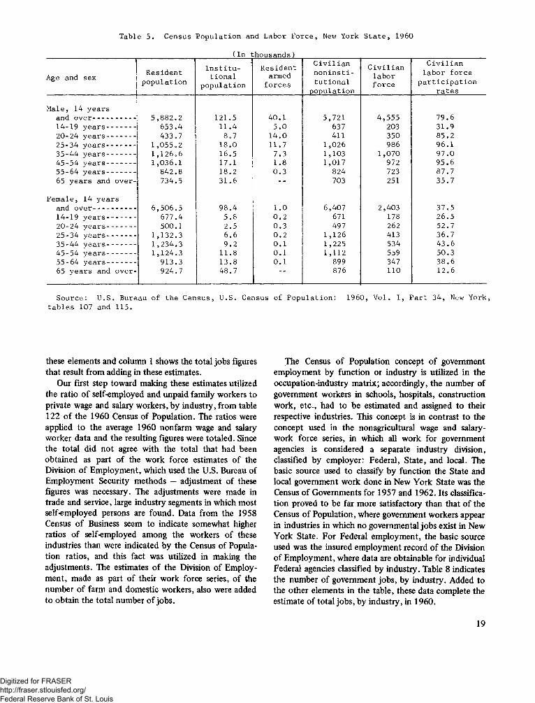
The basic 1960 Census of Population civilian labor force data for New York State, by age and sex, contained in table 5, were first adjusted to a Current Population Survey basis and then were further adjusted from the March-April 1960 Census period to a 1960 annual average basis. (See tables 6 and 7.) These adjustments were made by applying national relationships.
N onfarm wage and salary job s , b y in du stryA detailed set of figures by industry was essential,
since it is the framework necessary for utilizing the BLS industry-occupation matrix. Nonfarm job data for New York State for 1960 from the BLS-State program had been published for manufacturing in selected 2-digit, 3-digit, and 4-digit detail and for nonmanufacturing in 1-digit and 2-digit detail. For some nonmanufacturing industries, particularly in services, greater detail than had been published was necessary. Most of the data was obtained from unpublished estimates of the Office of Research and Statistics of the New York State Division of Employment. In the few cases where such figures were not available, estimates were made by interpolating between the 1959 and the 1962 data of C ou n ty Business Patterns. The resulting number of nonfarm wage and salary jobs is shown in the second column of table 8, which is limited to 2-digit industry detail.T ota l jo b s , b y in du stry
The BLS national matrix includes self-employed and unpaid family workers, farm employees, and domestic employees, in addition to nonfarm employment. Column 3 in table 8 shows New York State estimates for
18
Digitized for FRASER http://fraser.stlouisfed.org/ Federal Reserve Bank of St. Louis
T a b l e 5 . C e n s u s P o p u l a t i o n an d L a b o r F o r c e , New Y o r k S t a t e , I 9 6 0
( I n t h o u s a n d s )1A g e and s e x R e s i d e n t
p o p u l a t i o nI n s t i t u
t i o n a lp o p u l a t i o n
R e s i d e n tarm ed
f o r c e s
C i v i l i a nn o n i n s t i -t u t i o n a l
p o p u l a t i o n
C i v i l i a nl a b o rf o r c e
C i v i l i a n l a b o r f o r c e
p a r t i c i p a t i o n r a t e s
M a l e , 14 y e a r san d o v e r -------------------- 5 , 8 8 2 . 2 1 2 1 . 5 4 0 . 1 5 , 7 2 1 4 , 5 5 5 7 9 . 61 4 - 1 9 y e a r s ------------- 6 5 3 . 4 1 1 . 4 5 . 0 6 3 7 20 3 3 1 . 92 0 - 2 4 y e a r s ------------- 4 3 3 . 7 8 . 7 1 4 . 0 41 1 3 5 0 8 5 . 22 5 - 3 4 y e a r s .................. 1 , 0 5 5 . 2 1 8 . 0 1 1 . 7 1 ,0 2 6 9 8 6 9 6 . 13 5 - 4 4 y e a r s ------------- 1 , 1 2 6 . 6 1 6 . 5 7 . 3 1 , 1 0 3 1 , 0 7 0 9 7 . 04 5 - 5 4 y e a r s ------------- 1 , 0 3 6 . 1 1 7 . 1 1 .8 1 , 0 1 7 9 7 2 9 5 . 65 5 - 6 4 y e a r s ------------- 8 4 2 . 8 1 8 . 2 0 . 3 8 2 4 72 3 8 7 . 765 y e a r s and o v e r - 7 3 4 . 5 3 1 . 6 - - 7 0 3 251 3 5 . 7
F e m a l e , 14 y e a r sand o v e r ........................... 6 , 5 0 6 o 5 9 8 . 4 t i . o 6 , 4 0 7 2 , 4 0 3 3 7 . 51 4 - 1 9 y e a r s ------------- 6 7 7 . 4 5 . 8 0 . 2 671 1 7 8 2 6 . 52 0 - 2 4 y e a r s ------------- 5 0 0 . 1 2 . 5 0 . 3 4 9 7 262 5 2 . 72 5 - 3 4 y e a r s ------------- 1 , 1 3 2 . 3 6 .6 0 . 2 1 ,1 2 6 41 3 3 6 . 73 5 - 4 4 y e a r s ------------- 1 , 2 3 4 . 3 9 . 2 0 .1 1 , 2 2 5 5 3 4 4 3 . 64 5 - 5 4 y e a r s ------------- 1 , 1 2 4 . 3 1 1 .8 0 . 1 1 ,1 1 2 5 5 9 5 0 . 35 5 - 6 4 y e a r s ------------- 9 1 3 . 3 1 3 . 8 0 .1 8 9 9 3 4 7 3 8 . 665 y e a r s and o v e r - 9 2 4 . 7 4 8 . 7 8 7 6 110 1 2 .6
S o u r c e : U . S . B u r e a u o f t h e C e n s u s , U . S . C e n s u s o f P o p u l a t i o n : 1 9 6 0 , V o l . I , P a r t 3 4 , New Y o r k ,t a b l e s 1 0 7 and 1 1 5 .
these elements and column 1 shows the total jobs figures that result from adding in these estimates.
Our first step toward making these estimates utilized the ratio of self-employed and unpaid family workers to private wage and salary workers, by industry, from table 122 of the 1960 Census of Population. The ratios were applied to the average 1960 nonfarm wage and salary worker data and the resulting figures were totaled. Since the total did not agree with the total that had been obtained as part of the work force estimates of the Division of Employment, which used the U.S. Bureau of Employment Security methods — adjustment of these figures was necessary. The adjustments were made in trade and service, large industry segments in which most self-employed persons are found. Data from the 1958 Census of Business seem to indicate somewhat higher ratios of self-employed among the workers of these industries than were indicated by the Census of Population ratios, and this fact was utilized in making the adjustments. The estimates of the Division of Employment, made as part of their work force series, of the number of farm and domestic workers, also were added to obtain the total number of jobs.
The Census of Population concept of government employment by function or industry is utilized in the occupation-industry matrix; accordingly, the number of government workers in schools, hospitals, construction work, etc., had to be estimated and assigned to their respective industries. This concept is in contrast to the concept used in the nonagricultural wage and salary- work force series, in which all work for government agencies is considered a separate industry division, classified by employer: Federal, State, and local. The basic source used to classify by function the State and local government work done in New York State was the Census of Governments for 1957 and 1962. Its classification proved to be far more satisfactory than that of the Census of Population, where government workers appear in industries in which no governmental jobs exist in New York State. For Federal employment, the basic source used was the insured employment record of the Division of Employment, where data are obtainable for individual Federal agencies classified by industry. Table 8 indicates the number of government jobs, by industry. Added to the other elements in the table, these data complete the estimate of total jobs, by industry, in 1960.
19
Digitized for FRASER http://fraser.stlouisfed.org/ Federal Reserve Bank of St. Louis
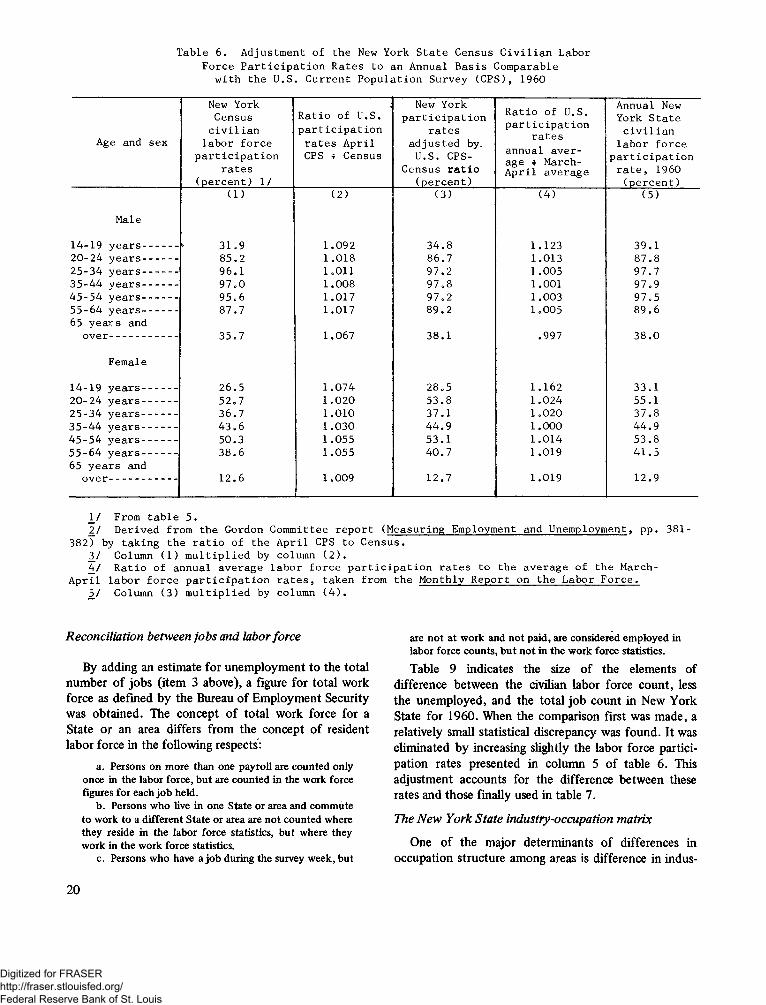
T a b l e 6 . A d j u s t m e n t o f t h e New Y o r k S t a t e C e n s u s C i v i l i a n L a b o r F o r c e P a r t i c i p a t i o n R a t e s t o an A n n u a l B a s i s C o m p a r a b l e
w i t h t h e U . S . C u r r e n t P o p u l a t i o n S u r v e y ( C P S ) , 1 9 6 0
A ge and s e x
New Y ork C e n s u s
c i v i l i a n l a b o r f o r c e
p a r t i c i p a t i o n r a t e s
( p e r c e n t ) 1 /
R a t i o o f U . S . p a r t i c i p a t i o n
r a t e s A p r i l CPS -r C e n s u s
New Y o r k p a r t i c i p a t i o n j
r a t e sa d j u s t e d by,
U . S . CPS- C e n s u s r a t i o
( p e r c e n t )
R a t i o o f U . S . p a r t i c i p a t i o n
r a t e sa n n u a l a v e r a g e 4 M a r c h - A p r i l a v e r a g e
A n n u a l New Y ork S t a t e
c i v i l i a n l a b o r f o r c e
p a r t i c i p a t i o n r a t e , 1 9 6 0
( p e r c e n t )( 1 ) ( 2 ) ( 3 ) ( 4 ) ( 5 )
M a le
1 4 - 1 9 y e a r s ----------- 3 1 . 9 1 . 0 9 2 3 4 . 8 1 . 1 2 3 3 9 . 12 0 - 2 4 y e a r s ----------- 8 5 . 2 1 . 0 1 8 8 6 . 7 1 . 0 1 3 8 7 . 82 5 - 3 4 y e a r s ----------- 9 6 . 1 1 .0 1 1 9 7 . 2 1 o 0 05 9 7 o 73 5 - 4 4 y e a r s ----------- 9 7 o0 1 . 0 0 8 9 7 o 8 1 .0 0 1 9 7 . 94 5 - 5 4 y e a r s ----------- 95 o 6 1 . 0 1 7 9 7 o 2 1 . 0 0 3 9 7 . 55 5 - 6 4 y e a r s ----------- 8 7 . 7 1 . 0 1 7 8 9 . 2 1 o0 0 5 8 9 . 665 y e a r s and
o v e r ---------------------- 35 o 7 1 . 0 6 7 3 8 . 1 . 9 9 7 3 8 . 0
F e m a le
1 4 - 1 9 y e a r s ----------- 2 6 . 5 1 . 0 7 4 28 o5 1 .1 6 2 3 3 . 12 0 - 2 4 y e a r s ----------- 52o 7 1 o 0 2 0 5 3 . 8 1 . 0 2 4 5 5 . 12 5 - 3 4 y e a r s ----------- 3 6 . 7 1 .0 1 0 3 7 . 1 1 .0 2 0 3 7 . 83 5 - 4 4 y e a r s ----------- 43 o 6 1 . 0 3 0 4 4 . 9 1 .0 0 0 4 4 . 94 5 - 5 4 y e a r s ----------- 5 0 . 3 1 . 0 5 5 5 3 . 1 1 . 0 1 4 5 3 . 85 5 - 6 4 y e a r s ----------- 3 8 . 6 1 . 0 5 5 4 0 . 7 1 . 0 1 9 4 1 . 565 y e a r s and
o v e r ---------------------- 1 2 .6 1 . 0 0 9 1 2 . 7 1 . 0 1 9 1 2 . 9
1 / From t a b l e 5 .2 ! D e r i v e d f r o m t h e G o r d o n C o m m i t t e e r e p o r t ( M e a s u r i n g E m p lo y m e n t an d U n e m p l o y m e n t , p p . 3 8 1 -
3 8 2 ) by t a k i n g t h e r a t i o o f t h e A p r i l CPS t o C e n s u s .3 / Colum n ( 1 ) m u l t i p l i e d by c o lu m n ( 2 ) .4 / R a t i o o f a n n u a l a v e r a g e l a b o r f o r c e p a r t i c i p a t i o n r a t e s t o t h e a v e r a g e o f t h e M a r ch -
A p r i l l a b o r f o r c e p a r t i c i p a t i o n r a t e s , t a k e n f r o m t h e M o n t h ly R e p o r t o n t h e L a b o r F o r c e .5 / C olum n ( 3 ) m u l t i p l i e d by c o lu m n ( 4 ) .
R econ cilia tion betw een jo b s and labor fo rce
By adding an estimate for unemployment to the total number of jobs (item 3 above), a figure for total work force as defined by the Bureau of Employment Security was obtained. The concept of total work force for a State or an area differs from the concept of resident labor force in the following respects:
a. Persons on more than one payroll are counted only once in the labor force, but are counted in the work force figures for each job held.
b. Persons who live in one State or area and commute to work to a different State or area are not counted where they reside in the labor force statistics, but where they work in the work force statistics.
c. Persons who have a job during the survey week, but
are not at work and not paid, are considered employed in labor force counts, but not in the work force statistics.Table 9 indicates the size of the elements of
difference between the civilian labor force count, less the unemployed, and the total job count in New York State for 1960. When the comparison first was made, a relatively small statistical discrepancy was found. It was eliminated by increasing slightly the labor force participation rates presented in column 5 of table 6. This adjustment accounts for the difference between these rates and those finally used in table 7.The N e w Y ork S ta te industry-occu pation m atrix
One of the major determinants of differences in occupation structure among areas is difference in indus-
2 0
Digitized for FRASER http://fraser.stlouisfed.org/ Federal Reserve Bank of St. Louis
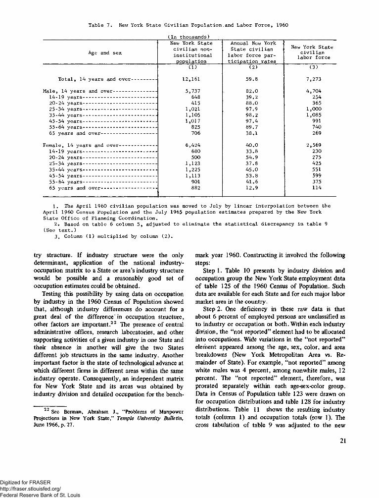
T a b l e 7 . New York S t a t e C i v i l i a n P o p u l a t i o n , and L a b or F o r c e , 1 9 60( I n t h o u s a n d s )
Age and s e xNew York S t a t e
c i v i l i a n n o n - i n s t i t u t i o n a l
p o p u l a t i o n
A nnual New York S t a t e c i v i l i a n
l a b o r f o r c e p a r t i c i p a t i o n r a t e s
New York S t a t e c i v i l i a n l a b o r f o r c e
( 1 ) ( 2 ) ( 3 )T o t a l , 14 y e a r s and o v e r ----------------- 1 2 ,1 6 1 5 9 . 8 7 , 2 7 3
M a le , 14 y e a r s and o v e r ----------------------------- 5 , 7 3 7 8 2 . 0 4 , 7 0 41 4 - 1 9 y e a r s ------------------------------------------------- 648 3 9 . 2 25 42 0 - 2 4 y e a r s .................................... ............................. 415 8 8 .0 3652 5 - 3 4 y e a r s - - ....................- ...................................- 1 ,0 2 1 9 7 . 9 1 ,0 0 03 5 - 4 4 y e a r s ------------------------------------------------- 1 , 1 0 5 9 8 . 2 1 , 0 8 54 5 - 5 4 y e a r s ------------------------------------------------- 1 , 0 1 7 9 7 . 4 9915 5 - 6 4 y e a r s - ......................... ..................... ................ 825 8 9 . 7 7 4 065 y e a r s and o v e r ------------------------------------- 70 6 3 8 . 1 269
F e m a l e , 14 y e a r s and o v e r ------------------------- 6 , 4 2 4 4 0 . 0 2 , 5 6 91 4 - 1 9 y e a r s ------------------------------------------------ 680 3 3 . 8 2 3 02 0 - 2 4 y e a r s ................. - ................- ..................... .. 5 0 0 5 4 . 9 2752 5 - 3 4 y e a r s .................................................................. 1 , 1 2 3 3 7 . 8 4253 5 - 4 4 y e a r s ...............- ............. .......... ........................ 1 , 2 2 5 4 5 . 0 5514 5 - 5 4 y e a r s ................. .......... ............................. ........ 1 , 1 1 3 5 3 . 8 5995 5 - 6 4 y e a r s ................. ..............................................- 901 4 1 . 6 37565 y e a r s and o v e r ------------------------------------- 882 1 2 . 9 11 4
1 . The A p r i l 1 9 6 0 c i v i l i a n p o p u l a t i o n was moved t o J u l y by l i n e a r i n t e r p o l a t i o n b e t w e e n t h e A p r i l 1 9 6 0 C e n su s P o p u l a t i o n and t h e J u l y 1965 p o p u l a t i o n e s t i m a t e s p r e p a r e d by t h e New York S t a t e O f f i c e o f P l a n n i n g C o o r d i n a t i o n .
2 . B a s e d on t a b l e 6 co lum n 5 , a d j u s t e d t o e l i m i n a t e t h e s t a t i s t i c a l d i s c r e p a n c y i n t a b l e 9 ( S e e t e x t . )
3 . Column ( 1 ) m u l t i p l i e d by co lum n ( 2 ) .
try structure. If industry structure were the only determinant, application of the national industry - occupation matrix to a State or area’s industry structure would be possible and a reasonably good set of occupation estimates could be obtained.
Testing this possibility by using data on occupation by industry in the 1960 Census of Population showed that, although industry differences do account for a great deal of the difference in occupation structure, other factors are important.22 The presence of central administrative offices, research laboratories, and other supporting activities of a given industry in one State and their absence in another will give the two States different job structures in the same industry. Another important factor is the state of technological advance at which different firms in different areas within the same industry operate. Consequently, an independent matrix for New York State and its areas was obtained by industry division and detailed occupation for the bench-
See Berman, Abraham J., “Problems of Manpower Projections in New York State,” Temple University Bulletin, June 1966, p. 27.
mark year 1960. Constructing it involved the following steps:
Step 1. Table 10 presents by industry division and occupation group the New York State employment data of table 125 of the 1960 Census of Population. Such data are available for each State and for each major labor market area in the country.
Step 2. One deficiency in these raw data is that about 6 percent of employed persons are unclassified as to industry or occupation or both. Within each industry division, the “not reported” element had to be allocated into occupations. Wide variations in the “not reported” element appeared among the age, sex, color, and area breakdowns (New York Metropolitan Area vs. Remainder of State). For example, “not reported” among white males was 4 percent, among nonwhite males, 12 percent. The “not reported” element, therefore, was prorated separately within each age-sex-color group. Data in Census of Population table 123 were drawn on for occupation distributions and table 128 for industry distributions. Table 11 shows the resulting industry totals (column 1) and occupation totals (row 1). The cross tabulation of table 9 was adjusted to the new
21
Digitized for FRASER http://fraser.stlouisfed.org/ Federal Reserve Bank of St. Louis
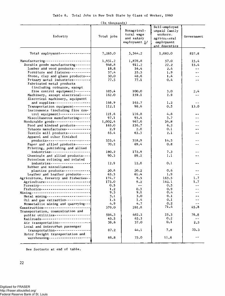
T a b l e 8 . T o t a l J o b s i n New Y o r k S t a t e by C l a s s o f W o r k e r , 1 9 6 0
( I n t h o u s a n d s )
I n d u s t r y
T o t a l e m p l o y m e n t --------------------------------
M a n u f a c t u r i n g -------------------------------------------------D u r a b l e g o o d s m a n u f a c t u r i n g ----------------
Lumber arid wood p r o d u c t s ------------------F u r n i t u r e an d f i x t u r e s ----------------------S t o n e , c l a y an d g l a s s p r o d u c t s -----P r i m a r y m e t a l i n d u s t r i e s ------------------F a b r i c a t e d m e t a l p r o d u c t s
( i n c l u d i n g o r d n a n c e , e x c e p tf i r e c o n t r o l e q u i p m e n t ) ----------------
M a c h i n e r y , e x c e p t e l e c t r i c a l ---------E l e c t r i c a l m a c h i n e r y , e q u i p m e n t
an d s u p p l i e s ---------------------------------------T r a n s p o r t a t i o n e q u i p m e n t ------------------I n s t r u m e n t s ( i n c l u d i n g f i r e c o n
t r o l e q u i p m e n t ) --------------------------------M i s c e l l a n e o u s m a n u f a c t u r i n g -----------
N o n d u r a b l e g o o d s ---------------------------------------F o o d a n d k i n d r e d p r o d u c t s ----------------T o b a c c o m a n u f a c t u r e s --------------------------T e x t i l e m i l l p r o d u c t s ------------------------A p p a r e l a n d o t h e r f i n i s h e d
p r o d u c t s -----------------------------------------------P a p e r an d a l l i e d p r o d u c t s ----------------P r i n t i n g , p u b l i s h i n g an d a l l i e d
i n d u s t r i e s -------------------------------------------C h e m i c a l s an d a l l i e d p r o d u c t s -------P e t r o l e u m r e f i n i n g an d r e l a t e d
i n d u s t r i e s .............................. - .........................R u b b e r an d m i s c e l l a n e o u s
p l a s t i c s p r o d u c t s ----------------------------L e a t h e r an d l e a t h e r p r o d u c t s ---------
A g r i c u l t u r e , f o r e s t r y an d f i s h e r i e s - -A g r i c u l t u r e --------------------------------------------------F o r e s t r y --------------------------------------------------------F i s h e r i e s ------------------------------------------------------
M i n i n g ----------------------------------------------------------------M e t a l m i n i n g -----------------------------------------------O i l a n d g a s e x t r a c t i o n --------------------------N o n m e t a l l i e m i n i n g an d q u a r r y i n g -----
C o n s t r u c t i o n ----------------------------------------------------T r a n s p o r t a t i o n , c o m m u n i c a t i o n an d
p u b l i c u t i l i t i e s ---------------------------------------R a i l r o a d s ------------------------------------------------------A i r t r a n s p o r t a t i o n -----------------------------------L o c a l an d i n t e r u r b a n p a s s e n g e r
t r a n s p o r t a t i o n ---------------------------------------M o to r f r e i g h t t r a n s p o r t a t i o n an d
w a r e h o u s i n g ---------------------------------------------
T o t a l j o b s
--------------------------------<N o n a g r i c u l - t u r a l w a g e a n d s a l a r y
e m p l o y m e n t JJ
1 S e l f - e m p l o y e d u n p a i d f a m i l y
w o r k e r s . a g r i c u i u u r a l
e m p l o y m e n t a n d d o m e s t i c s
G o v e r n m e n t
7 , 2 6 5 . 0 5 , 3 4 4 . 2 1 , 0 8 3 . 0 8 3 7 . 8
1 , 9 5 1 . 2 1 , 8 7 8 . 8 5 7 . 0 1 5 . 49 4 8 . 8 9 1 1 . 2 2 2 .2 1 5 . 4
18 o 8 1 6 . 4 2 . 43 7 . 4 3 5 . 5 1 . 95 0 . 0 4 8 . 6 1 . 47 7 . 5 7 7 . 1 0 . 4
1 0 5 . 4 1 0 0 .0 3 . 0 2 . 41 6 2 .0 1 5 9 . 1 2 . 9 - -
1 6 6 . 9 1 6 5 . 7 1 .2 __1 1 2 .1 9 8 . 6 0 . 5 1 3 . 0
1 2 1 .6 1 1 6 . 8 4 . 89 7 . 1 9 3 . 4 3 . 7 - -
1 , 0 0 2 . 4 9 6 7 . 6 3 4 . 8 - -1 6 3 . 0 1 5 6 . 7 6 . 3 - -
2 . 9 2 .8 0 .1 - -6 5 . 4 6 3 . 3 2 .1 - -
3 3 3 . 4 3 1 8 . 9 1 4 . 57 0 . 2 6 9 . 4 0 . 8
1 8 0 . 2 1 7 2 . 9 7 . 39 0 . 3 8 9 . 2 1 .1
1 2 . 9 1 2 .8 0 .1 - -2 0 .8 2 0 .2 0 . 66 3 . 3 6 1 . 4 1 . 9
1 7 4 . 7 9 . 5 1 6 3 . 5 1 . 71 7 3 . 0 9 . 2 1 6 2 . 1 1 . 7
0 . 5 0 . 5 - -1 .2 0 . 3 0 . 99 . 5 9 . 1 0 . 4 - -3 . 1 3 . 0 0 .1 - -1 . 5 1 . 4 0 .14 . 9 4 . 7 0 . 2
3 7 9 . 0 2 6 1 .8 7 1 . 4 4 5 . 8
5 8 4 . 3 4 8 2 . 2 2 5 . 3 7 6 . 86 5 . 5 6 5 . 3 0 . 23 9 . 6 3 7 . 0 0 . 1 2 . 5
8 7 . 2 4 4 . 1 7 . 8 3 5 . 3
8 6 .8 7 5 . 0 1 1 .8 - -
S e e f o o t n o t e a t e n d o f t a b l e .
2 2
Digitized for FRASER http://fraser.stlouisfed.org/ Federal Reserve Bank of St. Louis
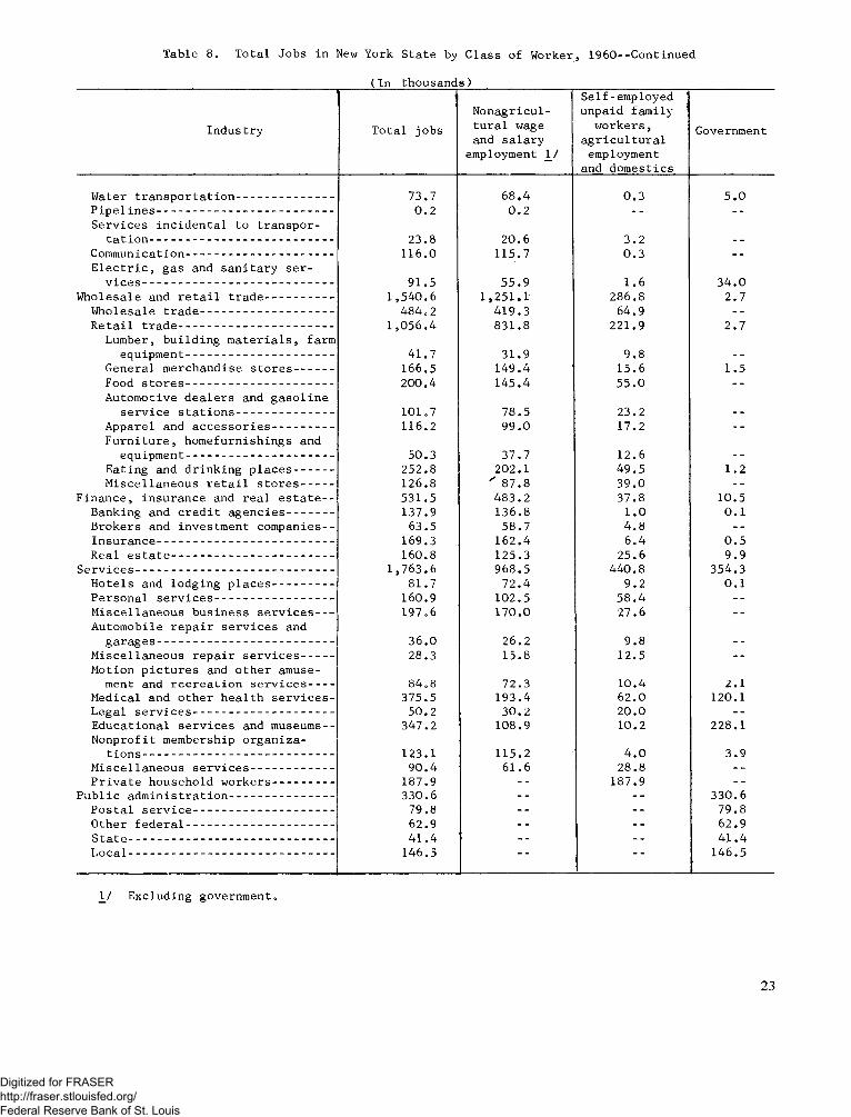
T a b l e 8 . T o t a l J o b s i n New Y o r k S t a t e b y C l a s s o f W o r k e r , 1 9 6 0 - - C o n t i n u e d
( I n t h o u s a n d s )
I n d u s t r y T o t a l j o b s
N o n a g r i c u l - t u r a l w a g e a n d s a l a r y
e m p l o y m e n t 1 /
S e l f - e m p l o y e d ' u n p a i d f a m i l } '
w o r k e r s , a g r i c u l t u r a l
e m p l o y m e n t a n d d o m e s t i c s
G o v e r n m e n t
W a t e r t r a n s p o r t a t i o n --------------------------------- 7 3 . 7 6 8 . 4 0 . 3 5 . 0P i p e l i n e s ------------------------------------------------------------- 0 . 2 0 . 2S e r v i c e s i n c i d e n t a l t o t r a n s p o r -
t a t i o n --------------------------------------------------------------- 2 3 . 8 2 0 . 6 3 . 2C o m m u n i c a t i o n --------------------------------------------------- 1 1 6 . 0 1 1 5 . 7 0 . 3E l e c t r i c , g a s a n d s a n i t a r y s e r -
v i c e s ------------------------------------------------------------------ 9 1 . 5 5 5 . 9 1 . 6 3 4 . 0W h o l e s a l e a n d r e t a i l t r a d e ----------------------- 1 , 5 4 0 . 6 1 , 2 5 1 . 1 2 8 6 . 8 2 . 7
W h o l e s a l e t r a d e ---------------------------------------------- 4 8 4 . 2 4 1 9 . 3 6 4 . 9 - -R e t a i l t r a d e ----------------------------------------------------- 1 , 0 5 6 . 4 8 3 1 . 8 2 2 1 . 9 2 . 7
L u m b e r , b u i l d i n g m a t e r i a l s , f a r m e q u i p m e n t --------------------------------------------------- 4 1 . 7 3 1 . 9 9 . 8 . .
G e n e r a l m e r c h a n d i s e s t o r e s ------------- 1 6 6 . 5 1 4 9 . 4 1 5 . 6 1 . 5F o o d s t o r e s --------------------------------------------------- 2 0 0 . 4 1 4 5 . 4 ; 5 5 . 0 - -A u t o m o t i v e d e a l e r s a n d g a s o l i n e
s e r v i c e s t a t i o n s --------------------------------- 1 0 1 o 7 7 8 . 5 2 3 . 2 . .
A p p a r e l a n d a c c e s s o r i e s --------------------- 1 1 6 . 2 9 9 . 0 1 7 . 2 - -F u r n i t u r e , h o m e f u r n i s h i n g s a n d
e q u i p m e n t --------------------------------------------------- 5 0 . 3 3 7 . 7 1 2 . 6 __
E a t i n g a n d d r i n k i n g p l a c e s ------------- 2 5 2 . 8 2 0 2 . 1 4 9 . 5 1 . 2M i s c e l l a n e o u s r e t a i l s t o r e s ----------- 1 2 6 . 8 ' 8 7 . 8 3 9 . 0 - -
F i n a n c e , i n s u r a n c e a n d r e a l e s t a t e - - 5 3 1 . 5 4 8 3 . 2 3 7 . 8 1 0 . 5B a n k i n g a n d c r e d i t a g e n c i e s ---------------- 1 3 7 . 9 1 3 6 . 8 1 . 0 0 . 1B r o k e r s a n d i n v e s t m e n t c o m p a n i e s - - 6 3 . 5 5 8 . 7 4 . 8I n s u r a n c e ------------------------------------------------------------- 1 6 9 . 3 1 6 2 . 4 6 . 4 0 . 5R e a l e s t a t e -------------------------------------------------------- 1 6 0 . 8 1 2 5 o 3 2 5 . 6 9 . 9
S e r v i c e s -------------------------------------------------------------------- 1 , 7 6 3 . 6 9 6 8 . 5 4 4 0 . 8 3 5 4 . 3H o t e l s a n d l o d g i n g p l a c e s --------------------- 8 1 . 7 7 2 . 4 9 . 2 0 . 1P e r s o n a l s e r v i c e s ----------------------------------------- 1 6 0 . 9 1 0 2 . 5 5 8 . 4 - -M i s c e l l a n e o u s b u s i n e s s s e r v i c e s ------ 1 9 7 . 6 1 7 0 . 0 2 7 . 6 - -A u t o m o b i l e r e p a i r s e r v i c e s a n d
g a r a g e s ------------------------------------------------------------- 3 6 . 0 2 6 . 2 9 . 8 __
M i s c e l l a n e o u s r e p a i r s e r v i c e s ----------- 2 8 . 3 1 5 . 8 1 2 . 5 - -M o t i o n p i c t u r e s a n d o t h e r a m u s e
m e n t a n d r e c r e a t i o n s e r v i c e s - ------ 8 4 . 8 7 2 . 3 1 0 . 4 2 . 1M e d i c a l a n d o t h e r h e a l t h s e r v i c e s - 3 7 5 . 5 1 9 3 . 4 6 2 . 0 1 2 0 . 1L e g a l s e r v i c e s ------------------------------------------------ 5 0 . 2 3 0 . 2 2 0 . 0E d u c a t i o n a l s e r v i c e s a n d m u s e u m s - - 3 4 7 . 2 1 0 8 . 9 1 0 . 2 2 2 8 . 1N o n p r o f i t m e m b e r s h i p o r g a n i z a -
t i o n s ------------------------------------------------------------------ 1 2 3 . 1 1 1 5 . 2 4 . 0 3 . 9M i s c e l l a n e o u s s e r v i c e s ---------------------------- 9 0 . 4 6 1 . 6 2 8 . 8P r i v a t e h o u s e h o l d w o r k e r s --------------------- 1 8 7 . 9 - - 1 8 7 . 9
P u b l i c a d m i n i s t r a t i o n ------------------------------------ 3 3 0 . 6 - - - - 3 3 0 . 6P o s t a l s e r v i c e ------------------------------------------------ 7 9 . 8 - - - - 7 9 . 8O t h e r f e d e r a l --------------------------------------------------- 6 2 . 9 - - 6 2 . 9S t a t e ----------------------------------------------------------------------- 4 1 . 4 - - - - 4 1 . 4L o c a l ----------------------------------------------------------------------- 1 4 6 . 5 1 4 6 . 5
1 / E x c l u d i n g g o v e r n m e n t , ,
23
Digitized for FRASER http://fraser.stlouisfed.org/ Federal Reserve Bank of St. Louis
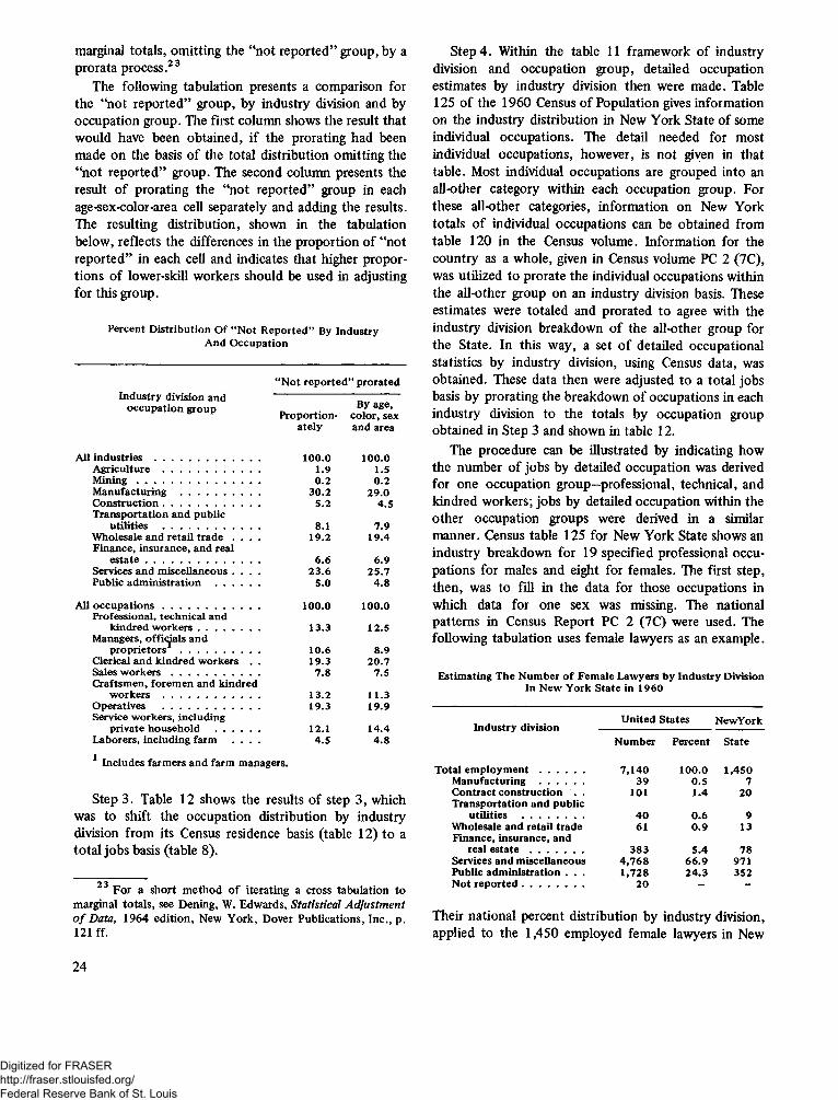
marginal totals, omitting the “not reported” group, by a prorata process.23
The following tabulation presents a comparison for the “not reported” group, by industry division and by occupation group. The first column shows the result that would have been obtained, if the prorating had been made on the basis of the total distribution omitting the “not reported” group. The second column presents the result of prorating the “not reported” group in each age-sex-color-area cell separately and adding the results. The resulting distribution, shown in the tabulation below, reflects the differences in the proportion of “not reported” in each cell and indicates that higher proportions of lower-skill workers should be used in adjusting for this group.
Percent Distribution O f “ Not R eported” By Industry And O ccupation
“ N ot reported ” proratedIndustry division and
occupation group Proportion By age, color, sex
ately and area
All industries ........................................... 1 0 0 .0 1 0 0 .0Agriculture ....................................... 1.9 1.5M in in g .................................................. 0 .2 0 .2Manufacturing ................................ 30 .2 29 .0C on stru ctio n ....................................... 5.2 4.5Transportation and publicutilities ....................................... 8.1 7.9W holesale and retail trade . . . . 19.2 19.4
Finance, insurance, and reale s t a t e .............................................. 6 .6 6.9
Services and m iscellaneous . . . . 23 .6 25 .7Public adm inistration .................. 5.0 4 .8All o c c u p a t io n s ....................................... 1 0 0 .0 1 0 0 .0Professional, technical and
kindred w o r k e rs ......................... 13 .3 12.5Managers, officials andproprietors1 ................................ 1 0 .6 8.9
Clerical and kindred workers . . 19 .3 20 .7Sales w o r k e r s .................................... 7 .8 7.5Craftsmen, forem en and kindredworkers ....................................... 13.2 11.3Operatives ....................................... 19 .3 19 .9Service workers, includingprivate household .................. 12.1 14.4
Laborers, including farm . . . . 4. 5 4. 81 Includes farmers and farm managers.
Step 3. Table 12 shows the results of step 3, which was to shift the occupation distribution by industry division from its Census residence basis (table 12) to a total jobs basis (table 8).
2 3 For a short method of iterating a cross tabulation to marginal totals, see Dening, W. Edwards, Statistical A dju stm en t o f Data, 1964 edition, New York, Dover Publications, Inc., p. 121 ff.
Step 4. Within the table 11 framework of industry division and occupation group, detailed occupation estimates by industry division then were made. Table 125 of the 1960 Census of Population gives information on the industry distribution in New York State of some individual occupations. The detail needed for most individual occupations, however, is not given in that table. Most individual occupations are grouped into an all-other category within each occupation group. For these all-other categories, information on New York totals of individual occupations can be obtained from table 120 in the Census volume. Information for the country as a whole, given in Census volume PC 2 (7C), was utilized to prorate the individual occupations within the all-other group on an industry division basis. These estimates were totaled and prorated to agree with the industry division breakdown of the all-other group for the State. In this way, a set of detailed occupational statistics by industry division, using Census data, was obtained. These data then were adjusted to a total jobs basis by prorating the breakdown of occupations in each industry division to the totals by occupation group obtained in Step 3 and shown in table 12.
The procedure can be illustrated by indicating how the number of jobs by detailed occupation was derived for one occupation group—professional, technical, and kindred workers; jobs by detailed occupation within the other occupation groups were derived in a similar manner. Census table 125 for New York State shows an industry breakdown for 19 specified professional occupations for males and eight for females. The first step, then, was to fill in the data for those occupations in which data for one sex was missing. The national patterns in Census Report PC 2 (7C) were used. The following tabulation uses female lawyers as an example.
Estimating The Number o f Fem ale Lawyers by Industry Division In N ew York State in 1960
Industry division
Total e m p lo y m e n t ..................Manufacturing ..................Contract construction . . Transportation and public
utilities .........................W holesale and retail trade Finance, insurance, and
real e s t a t e .....................Services and m iscellaneous Public adm inistration . . . N ot r ep o rted .........................
U nited States NewYorkNumber Percent State
7 ,14 0 1 0 0 .0 1,45039 0.5 7
101 1.4 2 0
40 0 .6 961 0 .9 13
383 5.4 784 ,7 6 8 66 .9 9711,728 24 .3 352
2 0 - -
Their national percent distribution by industry division, applied to the 1,450 employed female lawyers in New
24
Digitized for FRASER http://fraser.stlouisfed.org/ Federal Reserve Bank of St. Louis
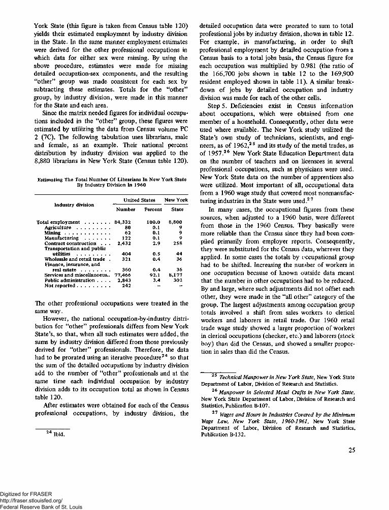
York State (this figure is taken from Census table 120) yields their estimated employment by industry division in the State. In the same manner employment estimates were derived for the other professional occupations in which data for either sex were missing. By using the above procedure, estimates were made for missing detailed occupation-sex components, and the resulting “other” group was made consistent for each sex by subtracting these estimates. Totals for the “other” group, by industry division, were made in this manner for the State and each area.
Since the matrix needed figures for individual occupations included in the “other” group, these figures were estimated by utilizing the data from Census volume PC 2 (7C). The following tabulation uses librarians, male and female, as an example. Their national percent distribution by industry division was applied to the 8,880 librarians in New York State (Census table 120).
Estimating The Total Number O f Librarians In N ew York State By Industry Division In 1960
U nited States N ew YorkIndustry division Number Percent State
Total e m p lo y m e n t ..................... 84 ,3 32 1 0 0 .0 8 ,800Agriculture ............................ 80 0.1 9M in in g ....................................... 62 0.1 9Manufacturing ..................... 1 2 2 0.1 9Contract construction . . . 2 ,432 2.9 258Transportation and public
utilities ............................ 40 4 0.5 44W holesale and retail trade . 321 0 .4 36Finance, insurance, and
real e s t a t e ......................... 360 0 .4 36Services and m iscellanoeus.. 77 ,4 66 92.1 8 ,177Public adm inistration . . . . 2 ,843 3.4 302N ot rep o rted ............................. 242 - -
The other professional occupations were treated in the same way.
However, the national occupation-by-industry distribution for “other” professionals differs from New York State’s, so that, when all such estimates were added, the sums by industry division differed from those previously derived for “other” professionals. Therefore, the data had to be prorated using an iterative procedure24 so that the sum of the detailed occupations by industry division add to the number of “other” professionals and at the same time each individual occupation by industry division adds to its occupation total as shown in Census table 120.
After estimates were obtained for each of the Census professional occupations, by industry division, the
24 Ibid.
detailed occupation data were prorated to sum to total professional jobs by industry division, shown in table 12. For example, in manufacturing, in order to shift professional employment by detailed occupation from a Census basis to a total jobs basis, the Census figure for each occupation was multiplied by 0.981 (the ratio of the 166,700 jobs shown in table 12 to the 169,900 resident employed shown in table 11). A similar breakdown of jobs by detailed occupation and industry division was made for each of the other cells.
Step 5. Deficiencies exist in Census information about occupations, which were obtained from one member of a household. Consequently, other data were used where available. The New York study utilized the State’s own study of technicians, scientists, and engineers, as of 1962,25 and its study of the metal trades, as of 1957.26 New York State Education Department data on the number of teachers and on licensees in several professional occupations, such as physicians were used. New York State data on the number of apprentices also were utilized. Most important of all, occupational data from a 1960 wage study that covered most nonmanufacturing industries in the State were used.27
In many cases, the occupational figures from these sources, when adjusted to a 1960 basis, were different from those in the 1960 Census. They basically were more reliable than the Census since they had been compiled primarily from employer reports. Consequently, they were substituted for the Census data, wherever they applied. In some cases the totals by occupational group had to be shifted. Increasing the number of workers in one occupation because of known outside data meant that the number in other occupations had to be reduced. By and large, where such adjustments did not offset each other, they were made in the “all other” category of the group. The largest adjustments among occupation group totals involved a shift from sales workers to clerical workers and laborers in retail trade. Our 1960 retail trade wage study showed a larger proportion of workers in clerical occupations (checker, etc.) and laborers (stock boy) than did the Census, and showed a smaller proportion in sales than did the Census.
25 Technical M anpower in N ew York S tate, New York State Department of Labor, Division of Research and Statistics.
26 M anpower in Selected M etal Crafts in N ew York State, New York State Department of Labor, Division of Research and Statistics, Publication B-107.
27 Wages and Hours in Industries Covered by the M inimum Wage Law, N ew York State, 1960-1961, New York State Department of Labor, Division of Research and Statistics, Publication B-132.
25
Digitized for FRASER http://fraser.stlouisfed.org/ Federal Reserve Bank of St. Louis
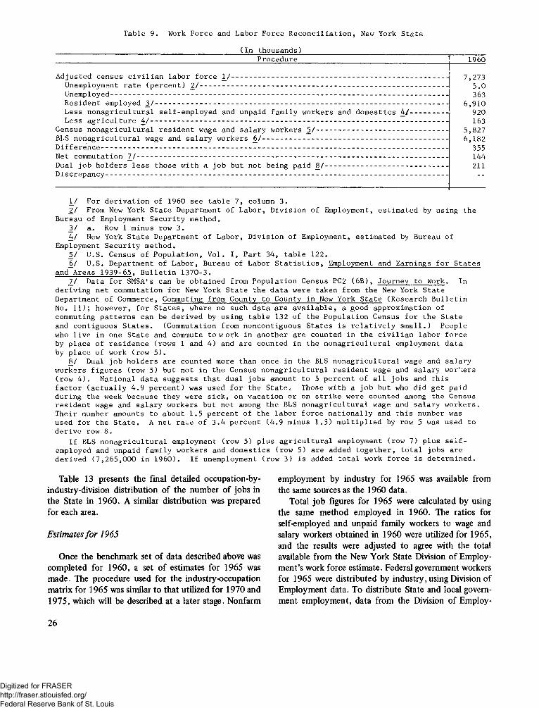
T a b l e 9 . W ork F o r c e a n d L a b o r F o r c e R e c o n c i l i a t i o n , New Y o r k S t a t e
( I n t h o u s a n d s )
A d j u s t e d c e n s u s c i v i l i a n l a b o r f o r c e \ _ / U n e m p l o y m e n t r a t e ( p e r c e n t ) £ / ----------------
P r o c e d u r e 1 9 6 0
7 , 2 7 35 oO
U n e m p l o y e d -------------------------------------------------------------------------------------------------------------------------------------------------------------------R e s i d e n t e m p l o y e d 3 1 ------------------------------------------------------------------------------------------------------------------------------------------L e s s n o n a g r i c u l t u r a l s e l f - e m p l o y e d a n d u n p a i d f a m i l y w o r k e r s a n d d o m e s t i c s 4 /L e s s a g r i c u l t u r e 4 / ---------------------------------------------------------------------------------------------------------------------------------------------
C e n s u s n o n a g r i c u l t u r a l r e s i d e n t w a g e a n d s a l a r y w o r k e r s 5 _ / --------------------------------------------------BLS n o n a g r i c u l t u r a l w a g e a n d s a l a r y w o r k e r s 6 / --------------------------------------------------------------------------------D i f f e r e n c e ------------------------------------------------------------------------------------------------------------------------------------------------------------------------N e t c o m m u t a t i o n 7 7 ----------------------------------------------------------------------------------------------------------------------------------------------------D u a l j o b h o l d e r s l e s s t h o s e w i t h a j o b b u t n o t b e i n g p a i d 8 / ---------------------------------------------
3 6 36 , 9 1 0
9 2 01 6 3
5 , 8 2 76 , 1 8 2
3 5 51 4 4211
D i s c r e p a n c y
1 / F o r d e r i v a t i o n o f 1 9 6 0 s e e t a b l e 7 , c o l u m n 3o2 / F r o m New Y o r k S t a t e D e p a r t m e n t o f L a b o r , D i v i s i o n o f E m p l o y m e n t , e s t i m a t e d b y u s i n g t h e
B u r e a u o f E m p l o y m e n t S e c u r i t y m e t h o d 03 / a . Row 1 m i n u s r o w 3 .4 / New Y o r k S t a t e D e p a r t m e n t o f L a b o r , D i v i s i o n o f E m p l o y m e n t , e s t i m a t e d b y B u r e a u o f
E m p l o y m e n t S e c u r i t y m e t h o d .5 / U . S . C e n s u s o f P o p u l a t i o n , V o l . I , P a r t 3 4 , t a b l e 1 2 2 .6 / U . S . D e p a r t m e n t o f L a b o r , B u r e a u o f L a b o r S t a t i s t i c s , E m p l o y m e n t a n d E a r n i n g s f o r S t a t e s
a n d A r e a s 1 9 3 9 - 6 5 , B u l l e t i n 1 3 7 0 - 3 .7 / D a t a f o r SMSA’ s c a n b e o b t a i n e d f r o m P o p u l a t i o n C e n s u s PC 2 ( 6 B ) , J o u r n e y t o W o r k . I n
d e r i v i n g n e t c o m m u t a t i o n f o r New Y o r k S t a t e t h e d a t a w e r e t a k e n f r o m t h e New Y o r k S t a t e D e p a r t m e n t o f C o m m e r c e , C o m m u t in g f r o m C o u n t y t o C o u n t y i n New Y o r k S t a t e ( R e s e a r c h B u l l e t i n N o . 1 1 ) ; h o w e v e r , f o r S t a t e s , w h e r e n o s u c h d a t a a r e a v a i l a b l e , a g o o d a p p r o x i m a t i o n o f c o m m u t i n g p a t t e r n s c a n b e d e r i v e d b y u s i n g t a b l e 1 3 2 o f t h e P o p u l a t i o n C e n s u s f o r t h e S t a t e a n d c o n t i g u o u s S t a t e s . ( C o m m u t a t i o n f r o m n o n c o n t i g u o u s S t a t e s i s r e l a t i v e l y s m a l l . ) P e o p l e w h o l i v e i n o n e S t a t e a n d c o m m u t e t o w o r k i n a n o t h e r a r e c o u n t e d i n t h e c i v i l i a n l a b o r f o r c e b y p l a c e o f r e s i d e n c e ( r o w s 1 a n d 4 ) a n d a r e c o u n t e d i n t h e n o n a g r i c u l t u r a l e m p l o y m e n t d a t a b y p l a c e o f w o r k ( r o w 5 ) .
8 / D u a l j o b h o l d e r s a r e c o u n t e d m o r e t h a n o n c e i n t h e BLS n o n a g r i c u l t u r a l w a g e a n d s a l a r y w o r k e r s f i g u r e s ( r o w 5 ) b u t n o t i n t h e C e n s u s n o n a g r i c u l t u r a l r e s i d e n t w a g e a n d s a l a r y w o r k e r s ( r o w 4 ) . N a t i o n a l d a t a s u g g e s t s t h a t d u a l j o b s a m o u n t t o 5 p e r c e n t o f a l l j o b s a n d t h i s f a c t o r ( a c t u a l l y 4 . 9 p e r c e n t ) w a s u s e d f o r t h e S t a t e . T h o s e w i t h a j o b b u t who d i d g e t p a i d d u r i n g t h e w e e k b e c a u s e t h e y w e r e s i c k , o n v a c a t i o n o r o n s t r i k e w e r e c o u n t e d am on g t h e C e n s u s r e s i d e n t w a g e a n d s a l a r y w o r k e r s b u t n o t am on g t h e BLS n o n a g r i c u l t u r a l w a g e a n d s a l a r y w o r k e r s . T h e i r n u m b e r a m o u n t s t o a b o u t 1 . 5 p e r c e n t o f t h e l a b o r f o r c e n a t i o n a l l y a n d t h i s n u m b e r w as u s e d f o r t h e S t a t e . A n e t r a t e o f 3 . 4 p e r c e n t ( 4 . 9 m i n u s 1 . 5 ) m u l t i p l i e d b y r o w 5 w a s u s e d t o d e r i v e r o w 8 .
I f BLS n o n a g r i c u l t u r a l e m p l o y m e n t ( r o w 5 ) p l u s a g r i c u l t u r a l e m p l o y m e n t ( r o w 7 ) p l u s s e l f - e m p l o y e d a n d u n p a i d f a m i l y w o r k e r s a n d d o m e s t i c s ( r o w 5 ) a r e a d d e d t o g e t h e r , t o t a l j o b s a r e d e r i v e d ( 7 , 2 6 5 , 0 0 0 i n 1 9 6 0 ) . I f u n e m p l o y m e n t ( r o w 3 ) i s a d d e d t o t a l w o r k f o r c e i s d e t e r m i n e d .
Table 13 presents the final detailed occupation-by- industry-division distribution of the number of jobs in the State in 1960. A similar distribution was prepared for each area.E stim a te s f o r 1 9 6 5
Once the benchmark set of data described above was completed for 1960, a set of estimates for 1965 was made. The procedure used for the industry-occupation matrix for 1965 was similar to that utilized for 1970 and 1975, which will be described at a later stage. Nonfarm
employment by industry for 1965 was available from the same sources as the 1960 data.
Total job figures for 1965 were calculated by using the same method employed in 1960. The ratios for self-employed and unpaid family workers to wage and salary workers obtained in 1960 were utilized for 1965, and the results were adjusted to agree with the total available from the New York State Division of Employment’s work force estimate. Federal government workers for 1965 were distributed by industry, using Division of Employment data. To distribute State and local government employment, data from the Division of Employ-
26
Digitized for FRASER http://fraser.stlouisfed.org/ Federal Reserve Bank of St. Louis

ment and the Census Bureau’s Governments Division were utilized.28 Where no data were available, distributions from the 1962 Census of Governments were used.
The only new element that arose in estimating the data for 1965 was in the calculation of labor force by age and sex. For this purpose, a set of population estimates and projections at 5-year intervals by 5-year age-sex groups, compiled by the Cornell Aeronautical Laboratories for the State Office of Planning Coordination was utilized.29 These population estimates were adjusted to a noninstitutional civilian population basis by utilizing the information for 1960 and by assuming that the changes in these groups from 1960 to 1965 were the same in each age-sex group as those in the population as a whole. Labor force participation rates then were estimated, first by utilizing the change that occurred nationally in each age-sex cohort between 1960 and 1965.30 When these ratios to the population figures had been applied, the resulting estimate for total civilian labor force showed an increase of about 3.5 percent between 1960 and 1965. About 3.1 of the 3.5 percent represented the result of population changes, a fact derived by applying the 1960 participation rates to the 1965 population.
In contrast to the 3.5 percent change between 1960 and 1965 in estimated civilian labor force, there was a change of only 2.9 percent in estimated work force. The current population counts by age and sex could have been wrong, or the work force estimates could have been wrong. However, both possibilities seemed unlikely, because the work force estimates are in large part determined by actual measurement for the State and because the population estimates, except for net migration, are determined similarly. The discrepancy was sought in one of the other elements of the estimating process. Tremendous changes could have taken place in the net commutation pattern. However, this factor was discounted. The one remaining element of major significance was the assumption that New York’s labor force participation rates had changed between 1960 and 1965 at the same rate as those nationally. If this assumption was erroneous a reasonable set of figures with which to
28 See Public E m ploym en t in 1965 and City E m ploym en t in 1965. Also D istribution o f N ew York State Positions by C ounty and Agency, 1964, New York State Civil Service Commission.
29 Demographic Projections fo r N ew York S tate Counties, New York State Executive Department, Office of Planning Coordination.
30 Cooper, Sophia and Denis Johnston, “Labor Force Projections for 1970-80,” M onthly Labor Review , February 1965,p .130.
reconcile our 1960 and 1965 data by age, sex, and industry might be obtained by using changes in national participation rates, modified between 1960 and 1965, particularly for women. After the data were modified, a reconciliation for 1965 between the total number of jobs and the labor force was obtained similar to the one for 1960, given in table 9.
Projections for 1970 and 1975
L a b o r f o r c e a n d n o n fa rm e m p lo y m e n t p r o je c t io n s
The projections for 1970 and 1975 build on the base of population projections made for the State Office of Planning Coordination by the Cornell Aeronautical Laboratories, which were mentioned earlier. This set of projections had the advantage of presenting figures for each county of the State, so that area projections could be made on the same basis as for the State as a whole. They were amended to a civilian noninstitutional basis in a manner similar to that used for 1960.
Changes shown by national projections of labor force participation rates were now utilized to obtain a first approximation of the labor force in 1970 and 1975, and these figures were amended later by a method similar to that described in connection with the 1965 data to reconcile the labor force totals with the total job figures. Unemployment was assumed to average 4 percent for the State as a whole. In some areas, lower levels of unemployment appeared reasonable; in other areas, somewhat higher levels were used.
Several experimental procedures were used to project nonagricultural employment for 1970 and 1975. One approach was to use logarithmic regression, another to use linear regression. Both were applied to the Statewide employment data, and then both were applied to the State data as a percent of the United States data. The results of the four methods were compared and the decision was made to utilize as the basic regression model Log Y = a + bt, where Y represents for each industry the percent that New York’s employment is of national employment for each year of the period 1947-65, and t = time in years.
The proportions were projected to 1970 and 1975 and, because they were in terms of percent of national nonagricultural employment, were multiplied by the BLS national employment projections, on a 4-percent- unemployment-level base, to obtain projected employment in New York State for 1970 and 1975.
For industries where a more detailed breakdown than 2 digits was needed in manufacturing and 1 digit in
27
Digitized for FRASER http://fraser.stlouisfed.org/ Federal Reserve Bank of St. Louis
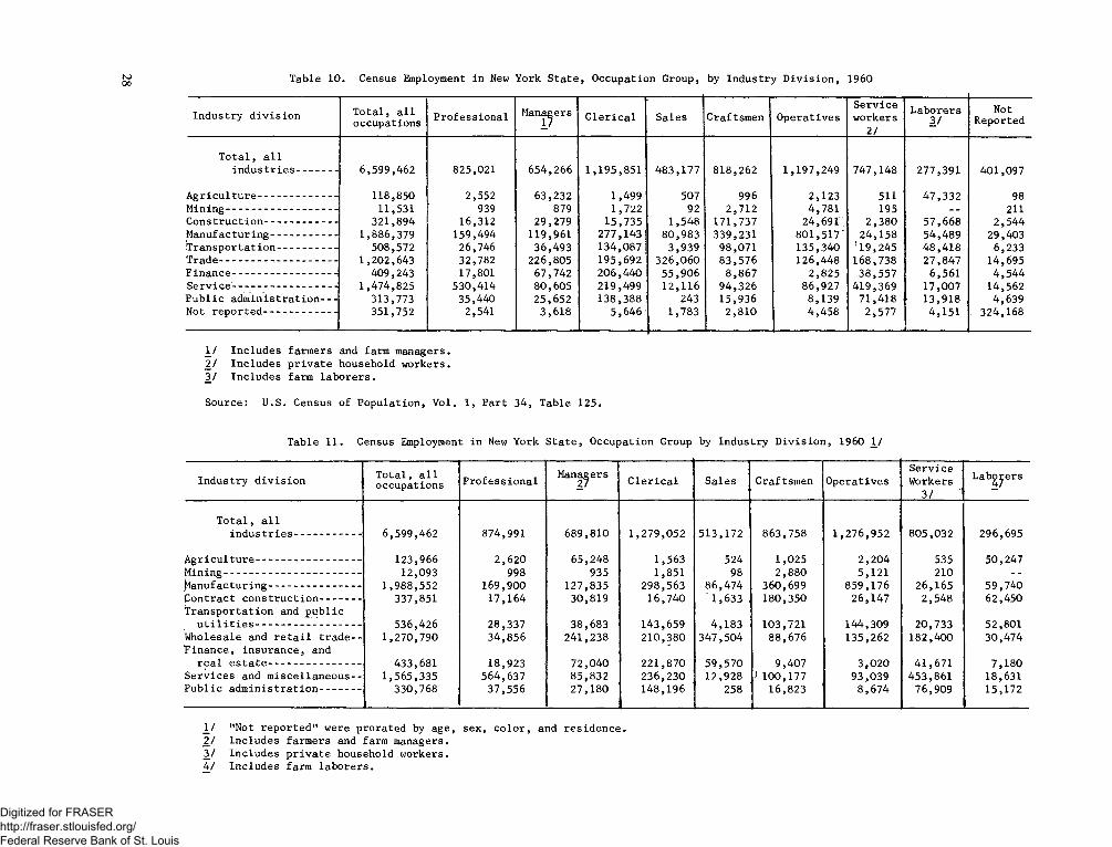
T a b le 1 0 . Census Employment i n New Y o r k S t a t e , O c c u p a t i o n G r o u p , by I n d u s t r y D i v i s i o n , 1960tooo
I n d u s t r y d i v i s i o n T o t a l , a l l o c c u p a t i o n s P r o f e s s i o n a l M anagers
1 / C l e r i c a l S a l e s C r a f t s m e n O p e r a t i v e sS e r v i c ew o r k e r s
2 /
L a b o r e r s3 /
NotR e p o r t e d
T o t a l , a l li n d u s t r i e s -------------- 6 , 5 9 9 , 4 6 2 8 2 5 ,0 2 1 6 5 4 , 2 6 6 1 , 1 9 5 , 8 5 1 4 8 3 , 1 7 7 8 1 8 , 2 6 2 1 , 1 9 7 , 2 4 9 7 4 7 , 1 4 8 2 7 7 , 3 9 1 4 0 1 , 0 9 7
A g r i c u l t u r e ---------------------------- 1 1 8 ,8 5 0 2 ,5 5 2 6 3 , 2 3 2 1 ,4 9 9 507 996 2 ,1 2 3 511 ; 4 7 , 3 3 2 98M i n i n g --------------------------------------- 1 1 ,5 3 1 939 879 1 ,7 2 2 92 2 , 7 1 2 4 ,7 8 1 195 211C o n s t r u c t i o n ........................... - 3 2 1 ,8 9 4 1 6 ,3 1 2 2 9 , 2 7 9 1 5 , 7 3 5 1 ,5 4 8 1 7 1 ,7 3 7 2 4 , 6 9 1 . 2 , 3 8 0 5 7 , 6 6 8 2 ,5 4 4M a n u f a c t u r i n g ----------------------- 1 , 8 8 6 , 3 7 9 1 5 9 ,4 9 4 1 1 9 ,9 6 1 2 7 7 ,1 4 3 | 8 0 , 9 8 3 3 3 9 , 2 3 1 8 0 1 , 5 1 7 2 4 , 1 5 8 5 4 , 4 8 9 2 9 ,4 0 3T r a n s p o r t a t i o n ...................... - 5 0 8 ,5 7 2 2 6 ,7 4 6 3 6 , 4 9 3 1 3 4 , 0 8 7 ! 3 ,9 3 9 9 8 , 0 7 1 1 3 5 , 3 4 0 '1 9 , 2 4 5 4 8 , 4 1 8 6 ,2 3 3T r a d e ----------------------------------------- 1 , 2 0 2 , 6 4 3 3 2 ,7 8 2 2 2 6 , 8 0 5 1 9 5 , 6 9 2 3 2 6 , 0 6 0 8 3 , 5 7 6 1 2 6 , 4 4 8 1 6 8 , 7 3 8 2 7 , 8 4 7 1 4 ,6 9 5F i n a n c e ................... - ..................... 4 0 9 ,2 4 3 1 7 ,8 0 1 6 7 , 7 4 2 2 0 6 , 4 4 0 5 5 , 9 0 6 8 , 8 6 7 2 ,8 2 5 3 8 , 5 5 7 6 ,5 6 1 4 , 5 4 4S e r v i c e ------------------------------------ 1 , 4 7 4 , 8 2 5 5 3 0 ,4 1 4 8 0 , 6 0 5 2 1 9 , 4 9 9 1 2 , 1 1 6 9 4 , 3 2 6 8 6 , 9 2 7 4 1 9 , 3 6 9 1 7 , 0 0 7 1 4 , 5 6 2P u b l i c a d m i n i s t r a t i o n ----- 3 1 3 ,7 7 3 3 5 ,4 4 0 2 5 , 6 5 2 1 3 8 , 3 8 8 * 243 1 5 , 9 3 6 8 , 1 3 9 7 1 , 4 1 8 1 3 , 9 1 8 4 ,6 3 9Not r e p o r t e d ------------------------- 3 5 1 ,7 5 2 2 ,5 4 1 3 ,6 1 8 5 , 6 4 6 1 ,7 8 3 2 , 8 1 0 4 , 4 5 8 2 ,5 7 7 4 ,1 5 1 . 3 2 4 , 1 6 8
1 / I n c l u d e s f a r m e r s and farm m a n a g e rs . 2 / I n c l u d e s p r i v a t e h o u s e h o l d w o r k e r s . 3 / I n c l u d e s fa r m l a b o r e r s .
S o u r c e : U .S . C e n su s o f P o p u l a t i o n , V o l . I , P a r t 3 4 , T a b l e 1 2 5 .
T a b l e 1 1 . Census Employment i n New Y o r k S t a t e , O c c u p a t i o n Group by I n d u s t r y D i v i s i o n , 1960 1 /
I n d u s t r y d i v i s i o n T o t a l , a l l o c c u p a t i o n s P r o f e s s i o n a l
M anagersC l e r i c a l S a l e s C r a f t s m e n O p e r a t i v e s
S e r v i c e W ork ers
3 / 1
L a b ^ y e r s
T o t a l , a l li n d u s t r i e s ----------------------- 6 , 5 9 9 , 4 6 2 8 7 4 ,9 9 1 6 8 9 , 8 1 0 1 , 2 7 9 , 0 5 2 5 1 3 , 1 7 2 8 6 3 , 7 5 8 1 , 2 7 6 , 9 5 2 8 0 5 , 0 3 2 2 9 6 , 6 9 5
A g r i c u l t u r e ------------------------------------ 1 2 3 ,9 6 6 2 , 6 2 0 6 5 , 2 4 8 1 ,5 6 3 5 24 1 ,0 2 5 2 , 2 0 4 535 5 0 , 2 4 7M i n i n g ........................................................ 1 2 ,0 9 3 998 935 1 ,8 5 1 98 2 , 8 8 0 5 ,1 2 1 210 - -(M a n u f a c tu r in g -------------------------------- 1 , 9 8 8 , 5 5 2 1 6 9 , 9 0 0 1 2 7 , 8 3 5 2 9 8 , 5 6 3 8 6 , 4 7 4 3 6 0 , 6 9 9 8 5 9 , 1 7 6 2 6 , 1 6 5 5 9 , 7 4 0C o n t r a c t c o n s t r u c t i o n -------------- 3 3 7 ,8 5 1 1 7 , 1 6 4 3 0 , 8 1 9 1 6 , 7 4 0 ' 1 , 6 3 3 1 8 0 , 3 5 0 2 6 , 1 4 7 2 ,5 4 8 6 2 , 4 5 0T r a n s p o r t a t i o n and p u b l i c
u t i l i t i e s ------------------------------------ 5 3 6 , 4 2 6 2 8 , 3 3 7 3 8 , 6 8 3 1 4 3 ,6 5 9 4 , 1 8 3 1 0 3 ,7 2 1 1 4 4 ,3 0 9 2 0 , 7 3 3 5 2 ,8 0 1W h o l e s a l e and r e t a i l t r a d e - - F i n a n c e , i n s u r a n c e , and
1 , 2 7 0 , 7 9 0 3 4 , 8 5 6 2 4 1 , 2 3 8 2 1 0 , 3 8 0 3 4 7 , 5 0 4 8 8 , 6 7 6 1 3 5 , 2 6 2 1 8 2 , 4 0 0 3 0 , 4 7 4
r e a l e s t a t e -------------------------------- 4 3 3 ,6 8 1 1 8 , 9 2 3 7 2 , 0 4 0 2 2 1 , 8 7 0 5 9 , 5 7 0 9 , 4 0 7 3 , 0 2 0 4 1 , 6 7 1 7 ,1 8 0S e r v i c e s and m i s c e l l a n e o u s - - 1 , 5 6 5 , 3 3 5 5 6 4 , 6 3 7 8 5 , 8 3 2 2 3 6 , 2 3 0 1 2 , 9 2 8 ; 1 0 0 , 1 7 7 9 3 , 0 3 9 4 5 3 , 8 6 1 1 8 ,6 3 1P u b l i c a d m i n i s t r a t i o n -------------- 3 3 0 , 7 6 8 3 7 , 5 5 6 2 7 , 1 8 0 1 4 8 ,1 9 6 258 1 6 , 8 2 3 8 , 6 7 4 7 6 , 9 0 9 1 5 ,1 7 2
1 / " N o t r e p o r t e d " w e r e p r o r a t e d by a g e , s e x , c o l o r , and r e s i d e n c e . 2 / I n c l u d e s f a r m e r s and fa rm m an ag e rs .3 / I n c l u d e s p r i v a t e h o u s e h o l d w o r k e r s .4 / I n c l u d e s fa r m l a b o r e r s .
Digitized for FRASER http://fraser.stlouisfed.org/ Federal Reserve Bank of St. Louis
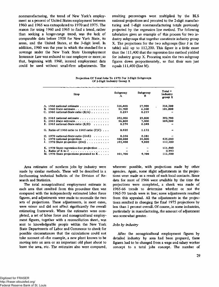
nonmanufacturing, the trend of New York’s employment as a percent of United States employment between 1960 and 1965 was extrapolated to 1970 and 1975. The reason for using 1960 and 1965 to find a trend, rather than seeking a longer-range trend, was the lack of comparable data before 1958 for New York State, its areas, and the United States, at the 3-digit level. In addition, 1960 was the year in which the standard for a coverage under the New York State Unemployment Insurance Law was reduced to one employee or more; so that, beginning with 1960, insured employment data could be used without small-firm adjustments. The
resulting percentages were multiplied by the BLS national projections and prorated to the 2-digit manufacturing and 1-digit nonmanufacturing totals previously projected by the regression line method. The following tabulation gives an example of this process for two industry subgroups that together constitute industry group X. The projections for the two subgroups (line J in the table) add up to 112,200. This figure is a little more than the 111 ,400 that the regression-line method yielded for industry group X. Prorating scales the two subgroup figures down proportionately, so that their sum just equals 111 ,400 (line M).
Projection O f T otal Jo b s To 1970 For 3-Digit Subgroups O f 2-Digit Industry G roup X
Step
A. 1960 national e s t im a te ........................................B. I9 6 0 S tate e s tim a te ...............................................C. 1960 national-S tate ra tio ( B /A ) ........................D. 1965 national e s t im a te ........................................E. 1965 S tate e s tim a te ...............................................F. 1965 national-S tate ra tio (E /D ) ....................G. R atio o f 1960 ra tio to 1965 ra tio (F /C ) . . .H. 1970 national-S tate ra tio (G xE) ....................I. 1970 national p rojection ..................................J. 1970 S tate p rojection ( H x l ) ..............................K. 1970 S tate regression-line p ro je c tio n ..............L. R atio o f K to J ......................................................M. 1970 S tate projections p ro rated to K ..............
Area estimates of nonfarm jobs by industry were made by similar methods. These will be described in a forthcoming technical bulletin of the Division of Research and Statistics.
The total nonagricultural employment estimate in each area that resulted from this procedure then was compared with the independently estimated labor force figures, and adjustments were made to reconcile the two sets of projections. These adjustments, in most cases, were minor and did not affect significantly the overall estimating framework. When the estimates were completed, a set of labor force and nonagricultural employment figures, together with a reconciliation sheet, was sent to knowledgeable people within the New York State Departments of Labor and Commerce to check for possible circumstances that the calculations could not take account of—for example, a new plant known to be moving into an area or an important old plant about to leave the area, etc. The estimates also were compared,
SubgroupA
SubgroupB
T otal = Industry group X
326 ,400 27 ,900 3 54 ,3009 5 ,700 6 ,100 101 ,800
0 .293 0 .219 -
352 ,900 29 ,800 3 82 ,70096 ,8 0 0 7,400 104 ,200
0 .2 7 4 0 .2 4 8 -
0 .935 1.132 -
0 .2 5 6 0.281 _4 0 0 ,0 0 0 35 ,000 43 5 ,0 0 0102 ,400 9 ,800 112 ,200
_ 111 ,400~ - 0 .993
101 ,700 9 ,700 111 ,400
wherever possible, with projections made by other agencies. Again, some slight adjustments in the projections were made as a result of such local contacts. Since data for most of 1966 were available by the time the projections were completed, a cheek was made of 1965-66 trends to determine whether or not the 1965-70 trends were in line; some adjustments resulted from this appraisal. All the adjustments in the projections resulted in changing the final 1975 projections by less than 1 percent overall. Of course, in some industries, particularly in manufacturing, the amount of adjustment was somewhat greater.Jo bs b y industry
After the nonagricultural employment figures by detailed industry by area had been prepared, these figures had to be changed from a wage and salary worker concept to a total jobs concept. The number of
29
Digitized for FRASER http://fraser.stlouisfed.org/ Federal Reserve Bank of St. Louis
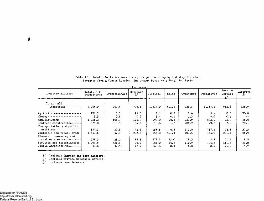
u>o
Table 12. Total Jobs in New York S tate, Occupation Group by Industry D ivision: Prorated from a Census Resident Employment Basis to a Total Job Basis
(In thousands)Industry d iv isio n Total, a l l occupations P rofessionals Managers C lerica l Sales Craftsmen Operatives
Serviceworkers2/
Laborers3 /
T otal, a l lin d u str ies--------------- 7,265.0 960.5 799.5 1 ,413 .0 601.2 921.5 1,317.8 912.6 338.9A griculture------------------------ 174.7 3.7 92.0 2.2 0 .7 1.4 3.1 0 .8 70.8Mining--------------------------------- 9.5 0.8 0 .7 1.4 0.1 2.3 4 .0 0 .2Manufacturing--------------------- 1,951.2 166.7 125.4 293.0 84.8 353.9 843.1 25.7 58.6Contract construction--------- 379.0 19.3 34.6 18.8 1.8 202.2 29.3 2.9 70.1Transportation and public
u t i l i t i e s --------------- --------- 584.3 30.9 42.1 156.5 4.6 113.0 157.1 22.6 57.5Wholesale and r e ta i l trade- 1,540.6 42.3 292.5 255.0 421.3 107.5 164.0 221.1 36.9Finance, insurance, and real e s ta te --------------------- 531.5 23.2 88.3 271.9 73.0 11.5 3.7 51.1 8 .8Services and m iscellaneous- 1,763.6 636.1 96.7 266.2 14.6 112.9 104.8 511.3 21.0Public adm inistration-------- 330.6 37.5 27.2 148.0 0.3 16.8 8.7 76.9 15.2
1/ Includes farmers and farm managers. 2/ Includes private household workers. 3 / Includes farm laborers.
Digitized for FRASER http://fraser.stlouisfed.org/ Federal Reserve Bank of St. Louis
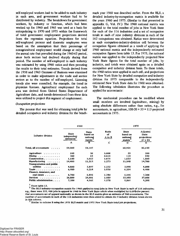
self-employed workers had to be added to each industry in each area, and government workers had to be distributed by industry. The breakdown for government workers, by industry or function, which had been worked up for 1960 and 1965 was used as a basis for extrapolating to 1970 and 1975 within the framework of total government employment projections derived from the regression equation. Projections for total self-employed persons and domestic employees were based on the assumption that their percentage of nonagricultural employment would change at only half the annual rate that prevailed during the 1960-65 period, since both sectors had declined sharply during that period. The number of self-employed in each industry was estimated by using 1960 ratios and then prorating the results to their total estimates. Trends derived from the 1958 and 1963 Censuses of Business were examined in order to make adjustments in the trade and service sectors as to the number of self-employed. Licensing trends also were consulted, for example, the trend in physician licenses. Agricultural employment for each area was derived from United States Department of Agriculture data, and trends determined from these data were utilized to project this segment of employment.Occupation projections
The process that was used for obtaining total jobs by detailed occupation and industry division for the bench
mark year 1960 was described earlier. From the BLS, a detailed industry-by-occupation matrix is available for the years 1960 and 1975. (Similar to that presented in appendix G, Vol. IV.) The 1960 national matrix was applied to the total number of jobs in New York State for each of the 116 industries and a set of occupation totals in each of nine industry divisions in each of the 162 occupations was obtained. Ratios were determined in each occupation-industry-division cell between the occupation figures obtained as a result of applying the 1960 national matrix and the independently estimated occupation figures from table 13. For 1975, the national matrix was applied to the independently projected New York State figures for the total number of jobs, by industry, and totals were obtained again on a detailed occupation and industry division basis. To these totals, the 1960 ratios were applied in each cell, and projections for New York State by detailed occupation and industry division for 1975 comparable to the independently estimated New York State data for 1960 were obtained. The following tabulation illustrates the procedure as applied for accountants:
The mechanical procedure can be modified where small numbers are involved (agriculture, mining) by using absolute differences rather than ratios, e.g., for accountants, in agriculture, 100-20 + 33 = 113 projected accountants in 1975.
I9 6 0 1975
Industry division Stateindependent
estim ates1
S tate based onnational . 2m atrix
Ratioo f
A to BState
based on national m atrix3
A djustedState
projections (C x D)
A B C D ETotal, all accountan ts .............. 69,800 58,187 68,925 82,100
A griculture ........................... 100 20 5.000 33 200M in in g ..................................... 300 65 4.615 114 500C o n s tru c tio n ........................... 1,100 1,023 1.075 1,633 1,800M anufacturing .................... 14,400 11,313 1.273 11,548 14,700T ransportation and public
utilities ........................... 4 ,800 3,897 1.232 3,898 4,800Trade ........................................ 6,400 6,214 1.030 6,254 6,400Finance, insurance, and
real e s t a t e ........................ 8 ,700 6,492 1.340 5,596 7,500Services .................................. 26,800 24,601 1.089 33,988 37,000Public adm inistra tion . . . . 7,200 4,562 1.578 5,861 9,2001 From table 13.2 The BLS industry-occupation m atrix fo r 1960 applied to to ta l jobs in New Y ork S tate in each o f 116 industries;
e.g., there were 333, 400 jobs in apparel in 1960 in New Y ork S tate which w hen m ultiplied by 0.09% -the percent th a t accountan ts are o f apparel nationally as shown in th e BLS matrix-gives an estim ate o f 300 accountan ts. The num ber o f accountan ts in each o f the 116 industries were th en added to obtain th e 9 industry division to ta ls shown in th is colum n.
3 Similar to colum n B using th e 1975 BLS m atrix and 1975 New Y ork S tate to ta l job projections.
31
Digitized for FRASER http://fraser.stlouisfed.org/ Federal Reserve Bank of St. Louis
After the projections were completed for all cells the figures were totaled and comparisons made between 1960 and 1975. In several cases, where occupation data were available for a series of years for New York State from other sources, independent projections were made and amendments were made in the projections that resulted from the mechanical process outlined above. Such data were available from licensing sources for doctors, dentists, and several other professional groups, and for teachers from the State Education Department. Independent projections were made for technicians by using the methods described in a report of the New York State Department of Labor on Technical Manpower in
New York State?1 A check also was made on the difference in 1950-60 trends by occupation in the nation and New York State as shown by 1950 and 1960 Census data, and these relationships also were utilized in amending the results of the matrix calculation.
For 1965 and 1970, occupation projections were obtained by a method similar to that used for 1975. A national matrix for these 2 years was necessary. It was devised by interpolating the 1960-75 proportions for each occupation in each industry.
31 Technical M anpower in N ew York State, vol. I, Supplement B, “Job Projections in Technical Occupations,” New York State Department of Labor, Division of Research and Statistics.
32
Digitized for FRASER http://fraser.stlouisfed.org/ Federal Reserve Bank of St. Louis
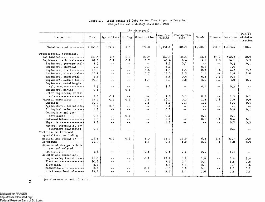
Table 13. Total Number of Jobs in New York State by D etailed Occupation and Industry D iv ision , 1960
(In thousands)Occupation —
Total Agriculture Milling Construction Manufacturing Transportation Trade Finance ServicesPublic
administra tionTotal occupation---------- 7,265.0 174.7 9.5 379.0 1,951.2 584.3 1,540.6 531.5 1,763.6 330.6
P ro fessio n a l, tech n ica l, and kindred----------------------- 930.5 4.5 0 .9 20.9 169.3 34.5 43.6 23.7 592.2 40.9Engineers, tech n ica l-------- 84.8 0.1 0.1 8.7 45.4 6.4 5.1 1.0 14.1 i 3.9Engineers, aeronautical- 1.7 -- 1.3 0.1 -- 0 .2 0.1Engineers, chemical------- 7.3 -- -- 0.7 5.2 -- 0 .4 -- 1.0Engineers, c i v i l ----------- 16.0 -- -- 5.6 1.3 1.5 0 .3 0 .4 4.7 : 2.2Engineers, e le c tr ic a l — 26.1 -- -- 0 .7 17.0 3.5 1.1 -- 2.8 1.0Engineers, ind ustria l — 5.8 -- -- 3 .6 0 .4 0 .5 0 .5 0 .8Engineers, mechanical— 22.8 -- -- 1.7 14.7 0 .8 2 .0 0.1 3 .0 0 .5Engineers, m etallurgi- c a l, e t c . .......................... 1.5 . . . . 1.1 0.1 __ 0 .3Engineers, mining---------- 0.1 -- 0.1 -- --Other engineers, techni-
c a l - - ................................... 3.5 0.1 1.2 0.1 0 .7 1.3 0.1Natural s c ie n t i s t s ----------- 17.9 0 .5 0.1 0.1 10.7 0 .3 1.3 0.1 3.9 0 .9Chemists------------------------ 10.2 -- 0.1 6.9 0 .3 1.1 -- 1.4 0 .4A gricultural s c ie n t is ts - 0.7 0.5 -- -- 0 .2 -- -- --B io log ica l s c ie n t i s t s — 1.7 -- -- 0 .7 -- -- 0.9 0.1G eologists and geo-p h y s ic is ts .................. --- 0 .4 0.1 0.1 0.1 0.1Mathematicians-------------- 1.8 -- 1.1 -- 0.1 0.1 0 .4 0.1P h y s ic is ts ............................. 2.7 -- -- 1.7 -- 0 .7 0 .3Natural s c ie n t i s t s , not elsewhere c la s s if ie d -- 0.4 . . . . _ _ 0 .4Technical workers and s p e c ia l is t s , excluding
medical and dental 1 / ......... 124.8 0.1 0.1 8.0 58.7 15.9 6.2 2.3 22.7 10.8Draftsmen-------------------------- 21.0 -- -- 1.2 9.6 1.2 0 .6 0.1 8 .0 0 .3Structural design tech nicians and related s p e c ia l is t s ......... ................. 2.6 0.6 0 .5 0.1 0.1 1.3Electro and mechanical engineering technicians- 41.0 . . . . 0.1 23.4 8.8 2.9 4 .4 1.4E lectron ic--------------------- 10.6 -- -- 7.7 0 .4 0.1 -- 1.8 0 .6E le c tr ic a l- ........................... 8.5 -- -- 3.5 3.6 0.1 0.7 0 .6Mechanical...........................- 8.3 -- -- 0.1 6.5 0 .4 0.1 1.1 0.1Electro-m echanical-------- 13.6 5.7 4 .4 2.6 -- 0 .8 0.1
u>u>
See footnote at end of table.
Digitized for FRASER http://fraser.stlouisfed.org/ Federal Reserve Bank of St. Louis
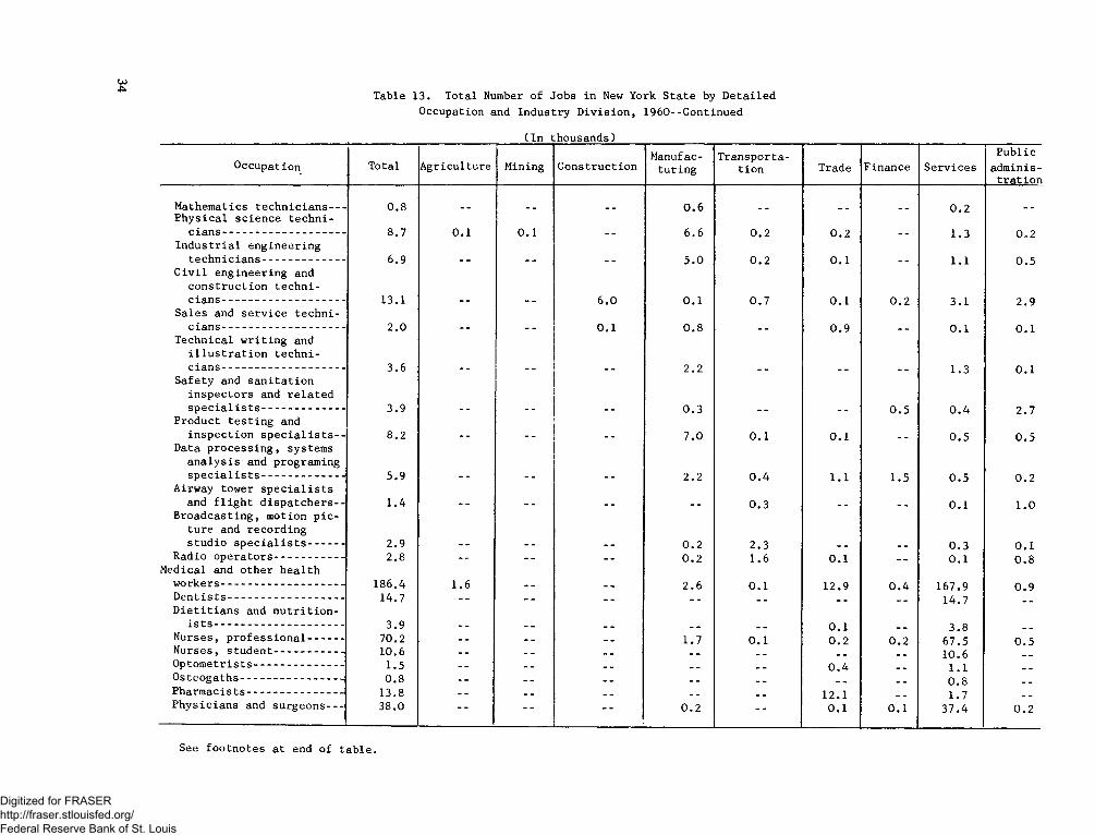
u>A Table 13. Total Number of Jobs in New York State by D etailed
Occupation and Industry D iv ision , I960--Continued________________________ (In thousands)__________________________
Occupation Total Agriculture Mining Construction Manufacturing Transportation Trade Finance ServicesPublic
administrationMathematics tech n ician s---- 0.8 0 .6 0 .2Physical science techni- c ian s---------- ------------------- 8.7 0.1 0.1 6.6 0 .2 0 .2 1.3 0.2Industria l engineering
tech n ician s-------------------- 6.9 5 .0 0 .2 0.1 1.1 0 .5C iv il engineering and construction techni- c ian s----------------------------- 13.1 6.0 0.1 0 .7 0.1 0 .2 3.1 2.9Sales and serv ice techni- c ian s----------------------------- 2.0 0.1 0 .8 0 .9 0.1 0.1Technical w riting and i l lu s tr a t io n techni- c ia n s----------------------------- 3.6 2.2 1.3 0.1Safety and san ita tion inspectors and related s p e c ia l is t s -------------------- 3.9 0 .3 0 .5 0 .4 2.7Product testin g andinspection s p e c ia l i s t s - - 8.2 . . 7.0 0.1 0.1 0 .5 0.5Data processing, systems an alysis and programing s p e c ia l is t s ................ .......... 5.9 2.2 0 .4 1.1 1.5 0.5 0 .2Airway tower s p e c ia l is t s and f l ig h t d isp a tch ers-- 1.4 0.3 0.1 1.0Broadcasting, motion p ic ture and recording studio s p e c ia l is t s -------- 2.9 0 .2 2.3 0.3 0.1Radio operators....................... 2.8 -- 0 .2 1.6 0.1 0.1 0 .8Medical and other health workers----------------------------- 186.4 1.6 2.6 0.1 12.9 0 .4 167.9 0.9D en tis ts ---------------------------- 14.7 -- -- _ _ _ _ 14.7 _
D ie tit ia n s and n u tr ition - i s t s .......................................... 3.9 0.1 3.8Nurses, p ro fessio n a l-------- 70.2 - - 1.7 0.1 0 .2 0 .2 67.5 0.5Nurses, student....................... 10.6 - - 10.6Optom etrists--------------------- 1.5 _ _ _ 0 .4 _ 1.1Osteogaths............- ................... 0.8 _ _ 0.8Pharmacists....... ..................... - 13.8 _ 12.1 _ 1.7Physicians and surgeons---- 38.0 0 .2 -- 0.1 0.1 37.4 0 .2
See footnotes at end of tab le .
Digitized for FRASER http://fraser.stlouisfed.org/ Federal Reserve Bank of St. Louis
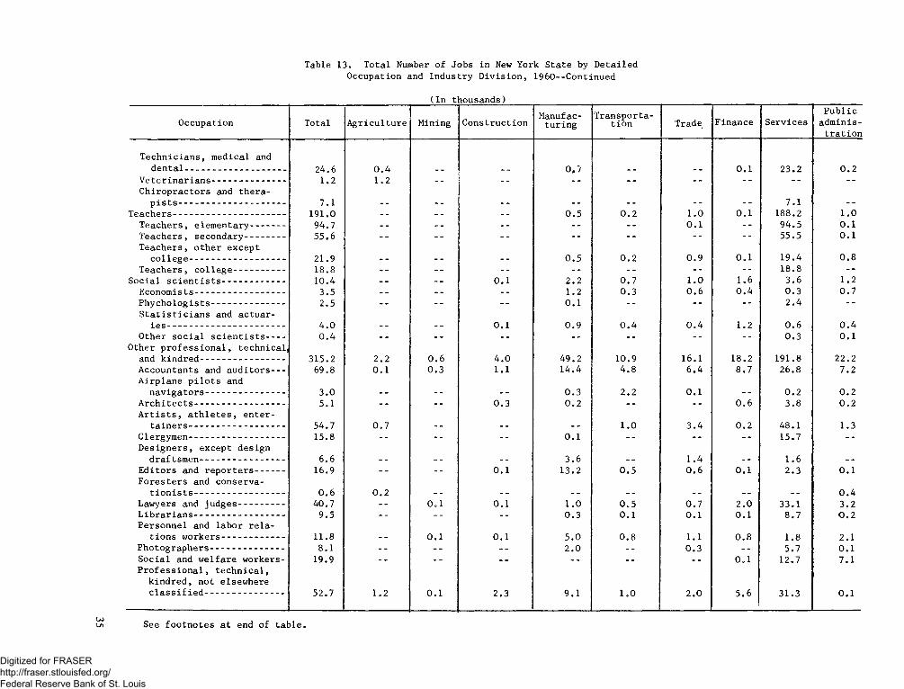
Table 13. Total Number of Jobs in New York State by Detailed Occupation and Industry D iv isio n , 1960--Continued
(In thousands)
Occupation Total A griculture Mining Construction Manufacturing
Transportation Trade Finance Services
Publicadminis
tration
Technicians, medical and dental..................- ............... 24.6 0.4 0,7 0.1 23.2 0.2
V eterinarians---------------------- 1.2 1.2 -- -- --Chiropractors and thera-
p is t s ........ ........... - ............... 7.1 7.1Teachers---------------------------------- 191.0 -- - - - - 0.5 0.2 1.0 0.1 188.2 1.0
Teachers, elementary---------- 94.7 -- - - -- 0.1 94.5 0.1Teachers, secondary............- 55.6 -- -- - - 55.5 0.1Teachers, other except
c o lle g e --------------------------- 21.9 0.5 0.2 0.9 0.1 19.4 0.8Teachers, c o lle g e --........ — 18.8 -- -- -- 18.8
Social s c ie n t is t s ...... ............ 10.4 -- 0.1 2.2 0.7 1.0 1.6 3.6 1.2Economists--------------------------- 3.5 -- - - 1.2 0.3 0.6 0.4 0.3 0.7Phychologists---------------------- 2.5 -- - - - - 0.1 -- - - - - 2.4S ta t is t ic ia n s and actuar-
ie s ----------------------------------- 4.0 0.1 0.9 0.4 0.4 1.2 0.6 0.4Other so cia l s c ie n t is t s ----- 0.4 0.3 0.1
Other professional, te ch n ica l and kindred------------------------- 315.2 2.2 0.6 4.0 49.2 10.9 16.1 18.2 191.8 22.2Accountants and auditors---- 69.8 0.1 0.3 1.1 14.4 4.8 6.4 8.7 26.8 7.2Airplane p ilo ts and
navigators------------------------ 3.0 _ _ _ 0.3 2.2 0.1 _ 0.2 0.2A rch ite cts--------------------------- 5.1 -- - - 0.3 0.2 0.6 3.8 0.2A r t is t s , a th le te s, enter-
ta in e rs------------------- --------- 54.7 0.7 1.0 3.4 0.2 48.1 1.3Clergymen----------------------------- 15.8 -- 0.1 -- -- 15.7 --Designers, except design
draftsmen------------ ------------ 6.6 . . 3.6 1.4 __ 1.6Editors and reporters--------- 16.9 -- 0.1 13.2 0.5 0.6 0.1 2.3 0.1Foresters and conserva-
t io n is t s - - ........................... 0.6 0.2 . . . . __ __ 0.4Lawyers and judges-.............. 40.7 -- 0.1 0.1 1.0 0.5 0.7 2.0 33.1 3.2L ib ra r ia n s --------------------------- 9.5 -- 0.3 0.1 0.1 0.1 8.7 0.2Personnel and labor re la -
tions workers------------------- 11.8 0.1 0.1 5.0 0.8 1.1 0.8 1.8 2.1Photographers........ ................. 8.1 -- 2.0 0.3 5.7 0.1Social and welfare workers- 19.9 0.1 12.7 7.1P ro fessio n a l, tech n ical,
kindred, not elsewhere c la s s if ie d ----------------------- 52.7 1.2 0.1 2.3 9.1 1.0 2.0 5.6 31.3 0.1
u> See footnotes at end of table
Digitized for FRASER http://fraser.stlouisfed.org/ Federal Reserve Bank of St. Louis
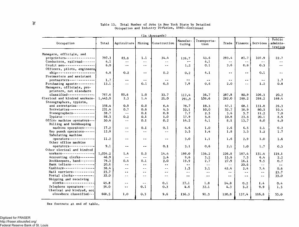
u>ON Table 13. Total Number of Jobs in New York State by Detailed Occupation and. Industry D iv is io n , 1960--Continued
(In thousands)
Occupation Total Agriculture Mining ConstructionManufac
turingTransporta
tion Trade Finance ServicesPublic
administration
Managers, o f f ic ia ls , andproprietors----- -------------------- 797.3 85.8 1.1 . 34.4 126.7 43.6 293.4 81.7 107.9 22.7Conductors, ra ilro a d ---------- 4.1 -- -- - - 4.1 -- --Credit men------------ --------------- 6.0 -- -- 1.2 0.1 3.6 0.8 0.3 --O ffice rs , p ilo ts , engineers,
ship---------------------------------- 4.8 0.2 . . 0.2 0.2 4.1 . . . . 0.1Postmasters and assistan t
postmasters---------------------- 1.7 _____ _____ _ _ _____ _____ _____ _____ 1.7Purchasing agents--------------- 13.1 -- 0.1 0.5 7.9 0.6 2.0 1.2 0.8Managers, o f f ic ia ls , pro
p rie to rs, not elsewhere c la s s if ie d ------------------------ 767.6 85.6 1.0 33.7 117.4 34.7 287.8 80.9 106.3 20.2
C le r ic a l and kindred workers- 1,443.0 2.3 1.4 21.0 291.9 156.6 282.0 269.2 269.2 149.4Stenographers, ty p is ts ,
and se cre ta rie s--------------- 358.4 0.9 0.8 6.4 78.7 18.3 47.1 68.1 111.8 26.3Se cre tarie s---------------------- 231.4 0.7 0.6 4.5 53.1 10.0 32.7 38.9 80.5 10.4Stenographers------------------- 38.7 -- 0.1 0.9 7.7 2.5 3.6 5.7 11.2 7.0T y p ists----------------------------- 88.3 0.2 0.1 1.0 17.9 5.8 10.8 23.5 20.1 8.9
O ffice machine operators---- 50.4 -- 0.1 0.2 14.2 4.1 8.1 13.7 6.0 4.0B il l in g and bookkeeping
machine operators--------- 17.2 . . 0.1 0.1 4.6 1.0 2.6 6.5 2.1 0.2Key punch operators--------- 12.9 -- -- - - 3.5 1.4 1.8 3.3 1.2 1.7Tabulating machine
operators---------------------- 11.2 . . _ _ 3.0 1.1 1.6 2.9 1.0 1.6Other o ffice machine
operators...... ................ 9.1 . . 0.1 3.1 0.6 2.1 1.0 1.7 0.5Other c le r ic a l and kindred
workers----------------------------- 1,034.2 1.4 0.5 14.4 199.0 134.2 226.8 187.4 151.4 119.1Accounting c le rk s ------------ 46.9 -- 2.4 9.6 3.2 15.6 7.5 6.4 2.2Bookkeepers, han d ---------- 79.3 0.4 0.1 2.0 19.9 2.7 27.9 16.1 9.5 0.7Bank t e lle r s --------------------- 20.6 -- - - 20.6C a sh ie rs --.......... - ........... . 58.4 ; -- - - - - 1.5 3.1 43.4 2.4 7 c 4 0.6Mail c a r r ie rs ------------------- 23.7 -- 23.7Postal c le rk s ------------------- 35.0 -- 35.0Shipping and receiving
c le rk s .... .......................... 45.8 _ _ 0.1 27.1 1.8 14.8 0.2 1.4 0.4Telephone operators--------- 56.0 0.1 0.3 4.6 32.1 4.3 3.2 9.9 1.5C le r ic a l and kindred, not
elsewhere c la s s if ie d - - - 668.5 1.0 0.3 9.6 136.3 91.3 120.8 137.4 116.8 55.0
See footnote at end of table.
Digitized for FRASER http://fraser.stlouisfed.org/ Federal Reserve Bank of St. Louis
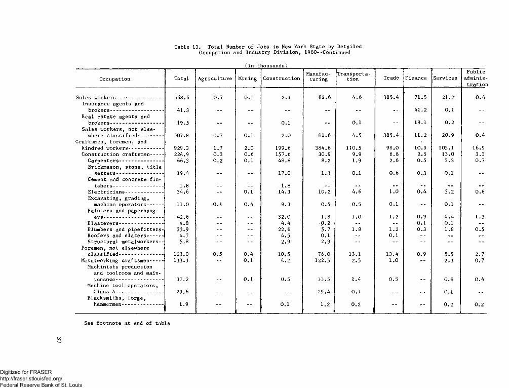
Table 13. Total Number of Jobs in New York State by Detailed Occupation and Industry D iv is io n , 1960--Continued
(In thousands)
Occupation Total Agricu lture Mining ConstructionManufac
turingTransporta
tion Trade Finance ServicesPublic
administration
Sales workers------------------------- 568.6 0.7 0.1 2.1 82.6 4.6 385.4 71.5 21.2 0.4Insurance agents and
brokers....................... ........ 41.3 41.2 0.1 _Real estate agents and
brokers.............. .................. 19.5 0.1 0.1 . . 19.1 0.2 . .Sales workers, not else-
where c la s s if ie d -------------- 507.8 0.7 0.1 2.0 82.6 4.5 385.4 11.2 20.9 0.4Craftsmen, foremen, and
kindred workers................... - 929.3 1.7 2.0 199.6 384.6 110.5 98.0 10.9 105.1 16.9Construction craftsmen------- 224.9 0.3 0.6 157.6 30.9 9.9 6.8 2.5 13.0 3.3
Carpenters........ .................. 66.3 0.2 0.1 48.8 8.2 1.9 2.6 0.5 3.3 0.7Brickmason, stone, t i t le
se tte rs------------------------- 19.4 17.0 1.3 0.1 0.6 0.3 0.1Cement and concrete f in -
ish e rs--------------------------- 1.8 1.8E le c tr ic ia n s ..................... - 34.6 0.1 14.3 10.2 4.6 1.0 0.4 3.2 0.8Excavating, grading,
machine operators--------- 11.0 0.1 0.4 9.3 0.5 0.5 0.1 0.1 _ _Painters and paperhang-
e rs..................................... 42.6 32.0 1.8 1.0 1.2 0.9 4.4 1.3P la ste re rs ------------------------ 4.8 __ -- 4.4 0.2 0.1 0.1Plumbers and p ip e fitte rs- 33.9 -- 22.6 5.7 1.8 1 c 2 0.3 1.8 0.5Roofers and s la te rs .......... 4.7 4.5 0.1 0.1 --Structura l metalworkers-- 5.8 -- 2.9 2.9 --
Foremen, not elsewherec la s s if ie d ------------------------ 123.0 0.5 0.4 10.5 76.0 13.1 13.4 0.9 5.5 2.7
Metalworking craftsmen------- 133.3 -- 0.1 4.2 122.5 2.5 1.0 -- 2.3 0.7Machinists production
and toolroom and main- tenance------------------------- 37.2 0.1 0.5 33.5 1.4 0.5 0.8 0.4
Machine tool operators, Class A.... ........... - ........... 29.6 29.4 0.1 0.1
Blacksm iths, forge,hammermen...... ................ - 1.9 -- -- 0 .! 1.2 0.2 -- -- 0.2 0.2
See footnote at end of table
Digitized for FRASER http://fraser.stlouisfed.org/ Federal Reserve Bank of St. Louis
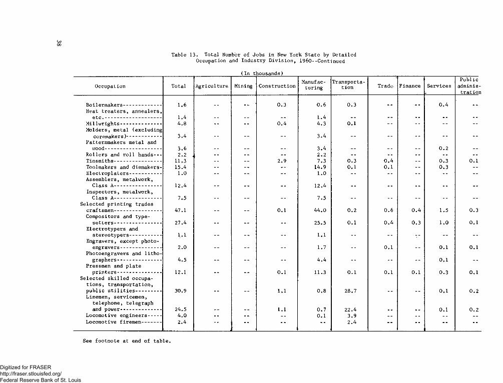
00
Table 13. Total Number of Jobs in New York State by Detailed Occupation and Industry D iv is io n , 1960--Continued
(In thousands)
Occupation Total Agriculture Mining ConstructionManufac
turingTransporta
tion Trade Finance ServicesPublic
administration
Boilermakers-------------------- 1.6 . . 0.3 0.6 0.3 . . . . 0 .4 . .Heat tre ate rs, annealers,
e t c .------------------------------- 1.4 1.4 . . . . . . . .M illw rights---------------------- 4.8 -- - - 0.4 4.3 0.1 -- -- - -Molders, metal (excluding
coremakers)...................... 3.4 _ _ _ 3.4 _ _ _ _Patternmakers metal and
wood------------------------------ 3.6 3.4 . . 0.2R o lle rs and r o ll hands---- 2.2 , -- - - 2.2 --Tinsm iths..................- ......... 11.3 -- -- 2.9 7.3 0.3 0.4 -- 0.3 0.1Toolmakers and diemakers- 15.4 -- -- 14.9 0.1 0.1 0.3E le ctro p la te rs----------------- 1.0 -- - - 1.0 --Assemblers, metalwork,
Class A-------------------------- 12.4 12.4Inspectors, metalwork,
Class A.............. - ............. 7.5 7.5Selected p rintin g trades
craftsmen------------------------- 47.1 0.1 44.0 0.2 0.6 0.4 1.5 0.3Compositors and type-
se tte rs------------------------- 27.4 25.5 0.1 0.4 0.3 1.0 0.1Electrotypers and
stereotypers----------------- 1.1 _ _ _ 1.1 _ _ _ _ _ _Engravers, except photo-
engravers---------------------- 2.0 _ 1.7 _ _ 0.1 _ 0.1 0.1Photoengravers and lith o -
graphers------------------------ 4.5 _ _ _ 4.4 _ _ _ 0.1Pressmen and plate
p rin te rs ...... ..................... 12.1 . . . . 0.1 11.3 0.1 0.1 0.1 0.3 0.1Selected s k il le d occupa
tion s, transportation, public u t i l i t i e s ................ 30.9 1.1 0.8 28.7 0.1 0.2Linemen, servicemen,
telephone, telegraph and power---------------------- 24.5 1.1 0.7 22.4 0.1 0.2
Locomotive engineers------- 4.0 -- -- - - 0.1 3.9 -- -- - - - -Locomotive firemen---------- 2.4 -- 2.4 --
i
See footnote at end of table.
Digitized for FRASER http://fraser.stlouisfed.org/ Federal Reserve Bank of St. Louis
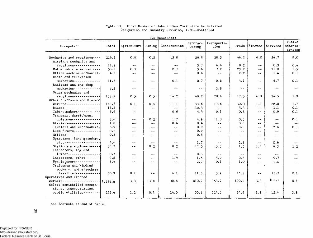
Table 13. Total Number of Jobs in New York State by Detailed Occupation and Industry D iv is io n , 1960--Continued
(In thousands)
Occupation Total Agricu lture Mining ConstructionManufac
turingTransporta
tion Trade Finance ServicesP ublic
administration
Mechanics and repairmen-----Airplane mechanics and
226.5 0.8 0.5 15.0 56.8 38.5 46.2 6.0 54.7 8.0
repairmen---------------------- 11.2 -- - - 3.7 6.6 0.2 0.3 0.4Motor vehicle mechanics-- 58.3 0.3 -- 0.7 3.6 7.2 23.2 21.8 1.5O ffice machine mechanics- Radio and te le v is io n
4.3 -- 0.6 2.2 1.4 0.1
mechanics----------------------Railroad and car shop
11.3 0.1 0.7 0.6 3.1 6.7 0.1
mechanics----------------------Other mechanics and
3.5 3.5
repairmen----------------------Other craftsmen and kindred
workers-------- -------------------Bakers.... ...................... .......
137.9
143.618.8
0.5
0.1
0.5
0.4
14.2
11.1
48.2
53.612.3
20.6
17.6
17.5
30.05.3
6.0
1.1
24.5
28.01.1
5.9
1.70.1
Cabinetmakers-------------------Cranemen, derrickmen,
6.9 0.6 4.4 0.1 0.8 0.9 0.1
hoistmen----------------------- 8.4 -- 0.2 1.7 4.9 1.0 0.5 -- 0.1G la z ie rs --------------------------- 1.8 -- 0.6 0.4 -- 0.8 --Jewelers and watchmakers- 6.9 -- -- -- 0.9 -- 3.3 - - 2.6 0.1Loom f ix e r s ---------------------- 0.2 -- 0.2 --M ille r s - - .............. - .............O pticians, lens grinders,
0.5 0.5
e t c . ................................... 4.4 -- 1.7 -- 2.1 0.6Stationary engineers-------•Inspectors, log and
28.3 0.2 0 o 2 12.5 5.3 1.5 1.1 6.3 1.2
lumber--------------------------- 0.3 0.3 -- -- - -Inspectors, other------------ 9.8 1.9 1.5 5.2 0.5 -- 0.7Upholsterers.......................Craftsmen and kindred
workers, not elsewhere
6.4 2.7 0.1 1.0 2.6
c la s s if ie d --------------------Operatives and kindred
50.9 0.1 6.1 11.3 5.9 14.2 13.2 0.1
workers.....................................Select sem iskilled occupa
tio n s, transportation,
1,285.8 3.3 3.8 30.4 810.7 153.7 170.2 3.9 101.7 8.1
public u t i l i t i e s -------------- 272.4 1.2 0.3 1 14.0 50.1 124.6i___________ ;
64.9'
1.1 12.4 3.8
See footnote at end of table.u>VO
Digitized for FRASER http://fraser.stlouisfed.org/ Federal Reserve Bank of St. Louis
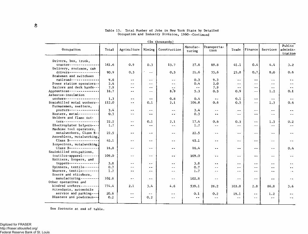
Table 13. Total Number of Jobs in New York State by Detailed Occupation and Industry D iv is io n , 1960--Continued
_______________________ (In thousands)_________________________
o
Occupation Total Agriculture Mining ConstructionManufac
turingTransporta
tion Trade F inance ServicesP ub lic
administratio n
D rivers, bus, truck,tra cto r-------------------------- 161.6 0.9 0.3 13.7 27.8 69.8 41.1 0.4 4.4 3.2
D elivery, routemen, cab d riv e rs -------------------------- 90.9 0.3 0*3 21.6 35.6 23.8 0.7, 8.0 0.6
Brakemen and switchmen ra ilro a d -------------- ---------- 9.6 0.3 9.3
Power station operators-- 2.4 -- - - 0.4 2.0 -- --S a ilo rs and deck hands---- 7.9 -- - - 7.9 --
Apprentices-------------------------- 16.7 -- -- 8 c9 5.3 0.3 0.9 -- 1.2 0.1A sbestos-insulation
workers................................. 1.3 . . 0.8 0.4 0.1Sem iskilled metal workers-- 112.0 -- 0.1 2.1 106.8 0.6 0.5 1.3 0.6
Furnacemen, sm elters, pourers-------------------------- 3.4 _ __ 3.4
Heaters, metal----------------- 0.3 0.3Welders and flame cut-
te rs ------------------------------- 22.2 0.1 2.1 17.4 0.6 0.5 1.3 0.2Ele ctro p late r helpers----- 1.7 -- -- 1.7Machine tool operators,
metalworkers, C lass B-- 22.5 . . 22.5Assemblers, metalworking,
Class B------------ ------------- 45.1 45.1Inspectors, metalworking,
Class B -........................... 16.8 16.4 0.4Sem iskilled occupations,
te x tile s-a p p a re l-------------- 109.0 109.0K n itte rs, loopers, and
toppers------------------------- 3.8 _ 3.8Spinners, t e x t i le ------------ 0.7 -- 0.7Weavers, t e x t i le -------------- 1.7 -- 1.7Sewers and s t itc h e rs ,
manufacturing--------------- 102.8 . . 102.8Other operatives and
kindred workers--------------- 774.4 2.1 3.4 4.6 539.1 28.2 103.8 2.8 86.8 3.6Attendants, automobile
service and parking----- 20.6 0.1 0.2 19.1 1.2Blasters and powdermen— 0.2 “ “ 0.2 —
See footnote at end of table
Digitized for FRASER http://fraser.stlouisfed.org/ Federal Reserve Bank of St. Louis
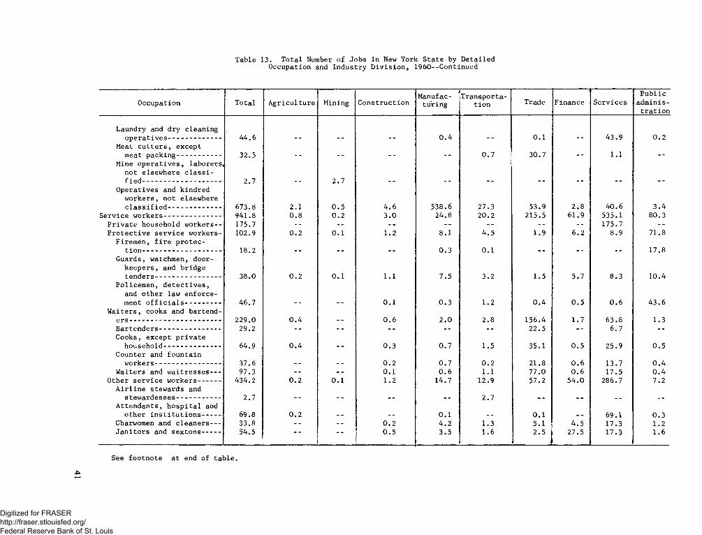
T a b l e 1 3 . T o t a l Number o f J o b s i n New Y o r k S t a t e b y D e t a i l e d O c c u p a t i o n a n d I n d u s t r y D i v i s i o n , 1 9 6 0 - - C o n t i n u e d
O c c u p a t i o n T o t a l A g r i c u l t u r e M i n i n g C o n s t r u c t i o n
jM a n u f a c
t u r i n gT r a n s p o r t a
t i o n T r a d e F i n a n c e S e r v i c e sP u b l i c
a d m i n i s t r a t i o n
L a u n d r y an d d r y c l e a n i n g o p e r a t i v e s ----------------------------- 4 4 . 6 0 . 4 0 . 1 4 3 . 9 0 . 2
M eat c u t t e r s , e x c e p tm e a t p a c k i n g - ....................... - 3 2 . 5 __ __ __ 0 . 7 3 0 . 7 1 . 1
M in e o p e r a t i v e s , l a b o r e r s , n o t e l s e w h e r e c l a s s i f i e d - ................................................ 2 . 7 2 . 7
O p e r a t i v e s a n d k i n d r e d w o r k e r s , n o t e l s e w h e r e c l a s s i f i e d ----------------------------- 6 7 3 . 8 2 . 1 0 . 5 4 . 6 5 3 8 . 6 2 7 . 3 5 3 . 9 2 . 8 4 0 . 6 3 . 4
S e r v i c e w o r k e r s ------------------------------- 9 4 1 . 8 0 . 8 0 . 2 3 . 0 2 4 . 8 2 0 . 2 2 1 5 . 5 6 1 . 9 5 3 5 . 1 8 0 . 3P r i v a t e h o u s e h o l d w o r k e r s - - 1 7 5 . 7 - - 1 7 5 . 7P r o t e c t i v e s e r v i c e w o r k e r s - 1 0 2 . 9 0 . 2 0 . 1 1 . 2 8 . 1 4 . 5 1 . 9 6 . 2 8 . 9 7 1 . 8
F i r e m e n , f i r e p r o t e c - t i o n ................................................... 1 8 . 2 0 . 3 0 . 1 __ 1 7 . 8
G u a r d s , w a t c h m e n , d o o r k e e p e r s , a n d b r i d g e t e n d e r s ------------------------------------ 3 8 . 0 0 . 2 0 . 1 1 . 1 7 . 5 3 . 2 1 . 5 5 . 7 8 . 3 1 0 . 4
P o l i c e m e n , d e t e c t i v e s , a n d o t h e r l a w e n f o r c e - m e n t o f f i c i a l s ------------------- 4 6 . 7 0 . 1 0 . 3 1 . 2 0 . 4 0 . 5 0 . 6 4 3 . 6
W a i t e r s , c o o k s a n d b a r t e n d - e r s ..................- ...................................... 2 2 9 . 0 0 . 4 0 . 6 2 . 0 2 . 8 1 5 6 . 4 1 . 7 6 3 . 8 1 . 3B a r t e n d e r s ............... - ..................... 2 9 . 2 - - - - - - 2 2 . 5 6 . 7 - -C o o k s , e x c e p t p r i v a t e
h o u s e h o l d ------------------------------- 6 4 . 9 0 . 4 . . 0 . 3 0 . 7 1 . 5 3 5 . 1 0 . 5 2 5 . 9 0 . 5C o u n t e r an d f o u n t a i n
w o r k e r s .......................................... 3 7 . 6 0 . 2 0 . 7 0 . 2 2 1 . 8 0 . 6 1 3 . 7 0 . 4W a i t e r s a n d w a i t r e s s e s — 9 7 . 3 - - - - 0 . 1 0 . 6 1 . 1 7 7 . 0 0 . 6 1 7 . 5 0 . 4
O t h e r s e r v i c e w o r k e r s ------------ 4 3 4 . 2 0 . 2 0 . 1 1 . 2 1 4 . 7 1 2 . 9 5 7 . 2 5 4 . 0 2 8 6 . 7 7 . 2A i r l i n e s t e w a r d s and
s t e w a r d e s s e s ------------------------ 2 . 7 2 . 7A t t e n d a n t s , h o s p i t a l and
o t h e r i n s t i t u t i o n s ............ 6 9 . 8 0 . 2 0 . 1 0 . 1 6 9 . 1 0 . 3C harw om en a n d c l e a n e r s ----- 3 3 . 8 - - - - 0 . 2 4 . 2 1 . 3 5 . 1 4 . 5 1 7 . 3 1 . 2J a n i t o r s a n d s e x t o n s ---------- 5 4 . 5 0 . 5 3 . 5 1 . 6 2 . 5 2 7 . 5 1 7 . 3 1 . 6
S e e f o o t n o t e a t e n d o f t a b l e
Digitized for FRASER http://fraser.stlouisfed.org/ Federal Reserve Bank of St. Louis
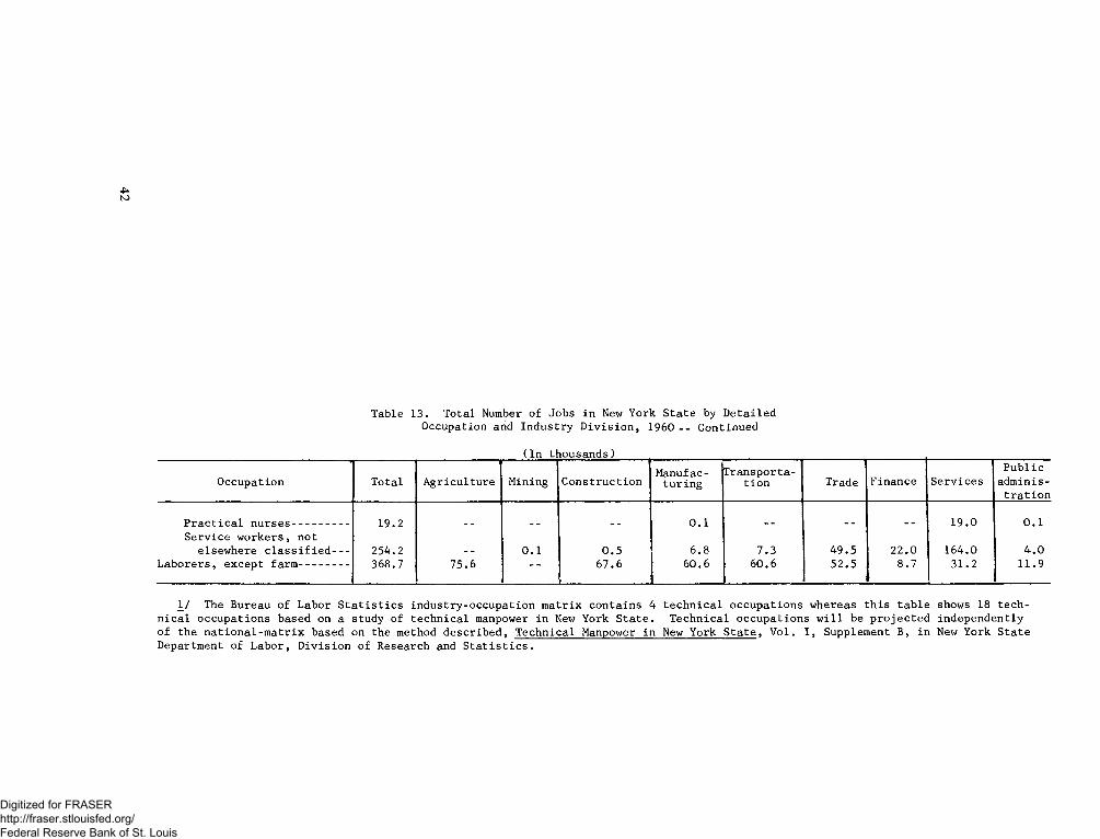
K)
T a b l e 1 3 . T o t a l Number o f J o b s i n New Y o r k S t a t e b y D e t a i l e d O c c u p a t i o n a n d I n d u s t r y D i v i s i o n , 1 9 6 0 - - C o n t i n u e d
( I n t h o u s a n d s )
O c c u p a t i o n T o t a l A g r i c u l t u r e M i n i n g C o n s t r u c t i o nM a n u f a c
t u r i n gT r a n s p o r t a
t i o n T r a d e F i n a n c e S e r v i c e sP u b l i c
a d m i n i s t r a t i o n
P r a c t i c a l n u r s e s -------------------- 1 9 . 2 0 . 1 _ _ 1 9 . 0 0 . 1S e r v i c e w o r k e r s , n o t
e l s e w h e r e c l a s s i f i e d ----- 2 5 4 . 2 0 . 1 0 . 5 6 . 8 7 . 3 4 9 . 5 2 2 . 0 1 6 4 . 0 4 . 0L a b o r e r s , e x c e p t f a r m ----------------- 3 6 8 . 7 7 5 . 6 6 7 . 6 6 0 . 6 6 0 . 6 5 2 . 5 , 8 . 7 3 1 . 2 1 1 . 9
1 / The B u r e a u o f L a b o r S t a t i s t i c s i n d u s t r y - o c c u p a t i o n m a t r i x c o n t a i n s 4 t e c h n i c a l o c c u p a t i o n s w h e r e a s t h i s t a b l e s h o w s 18 t e c h n i c a l o c c u p a t i o n s b a s e d o n a s t u d y o f t e c h n i c a l m an p ow er i n New Y o r k S t a t e . T e c h n i c a l o c c u p a t i o n s w i l l b e p r o j e c t e d i n d e p e n d e n t l y o f t h e n a t i o n a l - m a t r i x b a s e d o n t h e m e t h o d d e s c r i b e d , T e c h n i c a l M a n p ow er i n New Y o r k S t a t e , V o l . I , S u p p l e m e n t B , i n New Y o r k S t a t e D e p a r t m e n t o f L a b o r , D i v i s i o n o f R e s e a r c h and S t a t i s t i c s .
Digitized for FRASER http://fraser.stlouisfed.org/ Federal Reserve Bank of St. Louis
R ep la cem en t and J o b M o b ility
After expected growth or decline in the number of jobs by occupation has been found, the number of deaths and retirements, estimated from working-life tables computed by BLS for the Nation on the basis of 1960 patterns, are added. (See appendix A.) The patterns were applied to Census occupation distributions, by age and sex, for the State and its areas. The resulting rates were applied to an average of the number in the occupation in 1960 at the beginning and in 1975 at the end of the period and, thus, a reasonable approximation can be made of the number of job vacancies that can be expected as a result of deaths and retirements from the work force during 1960-75.32
To complete the picture, an estimate should be made of the number of jobs that will be created in each occupation by job shifts as people move up and down the occupational ladder. This area of job mobility is a most important one in terms of job replacement needs, particularly at lower occupation levels, and a great deal of research is needed to determine its extent. The present state of information available on this subject may result in crude estimates of this factor, possibly limited to occupational groups only.Conclusions
The problem of future manpower projections is like a jig-saw puzzle in which many important pieces are missing, particularly when attempts to make such projections for a State and its areas are made. However, a great many pieces can be fitted together and, with better data and techniques, in the future, some of the missing pieces possibly will be found. Although previous national, State, and New York City projections may have been off the mark in absolute dimension, they did point out fairly well the direction of change in the various occupational fields and they have illuminated the problems in the manpower field during the 1960’s.A future publication of the Division of Research and Statistics will present the method of the projection process used for New York State in greater detail.O th er S tu dies
Many other analytical manpower studies3 3 have been undertaken recently to develop methods and project manpower characteristics at subnational levels. Several of these studies are discussed briefly below.
32 Ibid, p. 14 ff.
A major work in the field of regional employment analysis has been published in eight (regional) volumes by the U.S. Department of Commerce34. The information presented in these volumes is designed to provide those concerned with the economy of an area, State and county, with a factual basis for comparing its past performance with that of other areas. The data used are taken from the Censuses of Population for 1940, 1950, and 1960. The technique used by the Commerce Department is built on the assumption that two basic facts about a region’s growth situation are necessary: the growth rate of the industrial m ix (distribution of industries) and, the size and growth of the regional share in this industrial distribution.
The rate of growth of a particular national industry is characterized as rapid if it exceeds and slow if it falls short of the growth rate of all national industries combined over the same period. The rate of growth of an industry within a particular region is characterized as rapid if it exceeds and slow if it falls short of the growth rate of that industry nationally. Since both the industrial-mix and the regional-share factors are at work simultaneously, they may be either mutually reenforcing or mutually offsetting. In some geographic areas both factors will be positive; in others both will be negative. In still other areas one factor will be positive and the other negative3 5.
The Battelle Memorial Institute has completed a study36 for the State of Michigan and the Detroit SMSA. The study develops and uses a complex procedure of integrated matrices to project the characteristics
33 Analytical manpower studies are based primarily on the analysis of historical data available from ongoing data collection systems. These studies may be contrasted with survey techniques which result in projections based primarily upon employer intentions.
34 Growth Patterns in E m ploym en t by County 1940-50 and 1950-60, U.S. Department of Commerce, Office of Business Economics, 1965, (8 vol.: New England $.45, Mideast $.65, Great Lakes $1.50, Plains $1.75, Southeast $2.75, Southwest $1.50, Rocky Mountain $.75, and Far West $.60.), Superintendent of Documents, U.S. Government Printing Office, Washington, D.C., 20402.
35 Although techniques for projecting industry employment are not included in these reports, considerable insight into the dynamics of regional growth can be gained from comparing the structure of growth in regions.
36 Michigan M anpower S tudy, prepared for the State of Michigan by the Battelle Memorial Institute, Columbus, Ohio, November 1966.
43
Digitized for FRASER http://fraser.stlouisfed.org/ Federal Reserve Bank of St. Louis
of the labor force (industry of employment, occupation of employment, and educational attainment) in 1970, 1975, and 1980. Essentially, the approach involved a reconciliation of the supply of and demand for labor, and used formal educational attainment as the equating variable. The model developed primarily involved the following steps:
(1) A projection of future demand for employees by occupation and industry and by educational attainment. (2) A projection of the future level of educational attainment of the population, by age and sex, and derivations from this projection of the future levels of educational attainment of the labor force37. (3) A reconciliation of the projected demand for and the supply of labor, in terms of educational attainment. The result was a profile of future employment by industry, occupation, and educational attainment.Industry employment levels were projected mainly by
a detailed analysis of key manufacturing industries and an examination of the relationship between the Michigan and U.S. economy, especially as the national economy was projected to 1975. Other techniques that were used included econometric analysis of historical trends, projections of employment levels in key industries based upon surveys, extrapolation of historical trends, and similar techniques. Occupational requirements were projected by obtaining a special tabulation of occupational employment from the 1960 Census of Population for Michigan and Detroit, and projecting it on the basis of detailed occupational trends at the national level and the trends represented by the 11 major occupational groups. These projected trends were modified in anticipation of technological changes and changes in the organization of individual industries over the projection period.An econometric approach to making projections for small area economies was developed by the Bureau of Business and Economic Research, Georgia State College, Atlanta, Georgia38. The purpose of this study was to develop a model for estimating future rates of migration, future levels of population, income, aggregate employment, and broad industry employment for counties or other small geographic areas. Because the time series data available for counties and other small areas was limited, use was made of cross-sectional data from many counties at two points in time. Specifically, the two
37 Population projections were available from a separatesource.
38 A Projections M odel fo r Small Area Economies, Roger L. Burford, Georgia State College, School of Business Administration, Bureau of Business and Economic Research, Atlanta, Ga., June 1966.
points were consecutive decennial census dates and the areas were 680 counties in the South. The model contains fourteen equations and was designed to reflect the dependence of population, employment, and other such variables in a small area on each other, upon income, the proximity of the area in question to a major city, and other relevant variables. The equations were solved simultaneously and the model provided projections for ten-year intervals corresponding to decennial census dates.
Economic base studies have been undertaken for a number of counties and cities in recent years. These studies usually divide the local economy into two segments: (1) Firms and individuals serving markets outside the community, export industries; and (2) Firms and individuals serving markets within the community, derivative industries. Export industries are considered the regulators of the level of economic activity and employment in an area. For example, when a local exporting coal mine closes, the impact is reflected in fewer sales of the local merchants to the jobless miners who have less to spend. The example illustrates how derivative activity is affected by changes in basic activity. As employment serving the export market rises or falls, employment serving the local market exhibits a positively correlated movement. Because of this “regulator” effect of export activity, an economic base study identifies the basic sources of employment and income, and provides a basis for understanding the source and level of all employment and income in a community.
The term “multiplier” frequently is used in base studies and refers to the impact that a change in the basic economic activity has on the aggregate level of activity within an economic unit. In the example above, basic dollars flowing into the area from sales of coal are multiplied into even greater local income through the process of spending and re-spending the basic dollars. As basic employment fluctuates, so does total employment change by some multiple, of the change in basic employment, the employment multiplier. likewise, as basic income fluctuates, so does total income change by some multiple, of the change in basic income, the income multiplier.
The purpose of one such economic base study39 was to provide guidance for the general economic development of a small county in West Virginia. From the
39 An Econom ic Profile o f Tucker County, W. V., James H. Land, West Virginia University, College of Commerce, Bureau of Business Research, Economic Development Series No. 10, January 1967.
44
Digitized for FRASER http://fraser.stlouisfed.org/ Federal Reserve Bank of St. Louis
economic base analysis for 1960 came an estimate of the employment multiplier—1.75. The multiplier suggested that for every 100 jobs in basic economic activity there were 75 jobs in derivative or “service” activity. From the theory underlying the multiplier analysis, the assumption is that for every additional 100 jobs in basic activity created in the area, 75 additional “service” jobs will develop.
A step-by-step approach to projecting long-run industry and occupational requirements in a region was the focus of another study40. Methods of determining whether a local industry’s employment is responsive mainly to local, State, or national demand are discussed, and several techniques for projecting industry employment corresponding to these influences are developed. Simple techniques for projecting occupational employment—primarily based on the relationship between local and national trends—are included. The importance of being familiar with current and expected changes in the environment of local industries so that judgment can be used to modify historical trends is emphasized in the report. Although the study was undertaken primarily to develop techniques adaptable to the data limitations of a small area, a case study for Silver Bow, Montana is presented in a separate volume.
The Bureau of Economic Research of The University of Colorado completed a study41 for the Department of Labor which explores techniques for projecting occupational requirements in an SMSA with consideration for data limitations. Six different approaches were examined—two “naive” and four “sophisticated”—and the implications of each were evaluated. One “best” approach was selected and developed comprehensively for the Denver SMSA. Projections were made for 20 occupations in 10 industries.
In projecting employment, a series of industry- occupational matrices were constructed corresponding to decennial census data. Employment-output functions
40 A Manual fo r the D evelopm ent o f Estim ates o f Future M anpower Requirem ents fo r Training Purposes, prepared by the Bureau of Economic and Business Research, Temple University, Philadelphia, Pa., for the Office of Manpower Policy, Evaluation and Research, U.S. Department of Labor, March 1966. In addition, see Projective M odels o f E m ploym en t by Industry and by Occupation fo r Small Areas: A Case S tu dy, also prepared by Temple University, March 1966.
41 M ethodology fo r Projection o f Occupational Trends in the Denver Standard M etropolitan Statistical Area, prepared for the Office of Manpower Policy, Evaluation, and Research, U.S. Department of Labor, by the Bureau of Economic Research, University of Colorado, Boulder, Colo., March 1966.
were developed for each industry. Output-time relations also were developed and used to make industry-output predictions. Judgments with respect to probable growth patterns of each industry were incorporated at this stage. Finally, the three phases were integrated into a complete model; output projections were related to production functions (output-employment relationships) to project future levels of industry employment which then were coupled with industry-occupational matrices to obtain projected occupational employment levels.
In a study42 for the Eastern Massachusetts region estimates of gross product by industry, employment by industry, wages and salaries by industry, and personal income and consumer expenditures were made for 5-year intervals from 1970 to 2000. The purpose of this study was to analyze past trends in development, to anticipate the direction of future development, and to identify specific means and programs for assisting this development.
Industry employment estimates were derived by first projecting the region’s constant dollar gross product by industry and then dividing the gross product by the projected value of gross product per worker in each industry. Projections of gross product for both national and local market industry groups were made by using regression techniques and least squares trend extentions of regional shares of markets. For example, gross product in 41 industries serving national markets were made by regressing regional industry gross product against a “demand” variable composed of related national GNP components and a “share” variable made up of the ratio proportion of regional to total national industry gross product. Theoretically, the demand variable accounted for growth in the industry, and the share variable accounted for the competitive position of the region in the Nation. In general, the assumption was that past trends in the region’s output per worker would continue over the projection period.
A variety of techniques were used to project population, labor force, and employment by industry and occupational group to 1975 in a study of potential demand and supply of manpower for the State of Indiana43. Two sets of employment projections were made. They corresponded to different assumptions of
42 Econom ic Base and Population S tudy fo r Eastern Massachusetts: Vol. I, Historical Analysis; Vol. II, Prospects fo r Econom ic Growth, Commonwealth of Massachusetts, Metropolitan Area Planning Council, 1967.
43 Indiana M anpower Trends to 1975, Indiana Employment Security Division, Research and Statistics, January 1967.
45
Digitized for FRASER http://fraser.stlouisfed.org/ Federal Reserve Bank of St. Louis
growth in GNP at the national level. Multiple regression techniques were used for projecting employment in several industries, which included construction and durable goods manufacturing, as were simple regressions, least squares extensions of historical employment series, and judgmental approaches in other industries. National trends in GNP, and output and output-per-worker by industry were important in determining employment by industry in the State.
Employment by occupational group was projected on the basis of changes in employment by industry between 1965 and 1975 and expected changes in the proportion of occupations in each industry group. Occupational proportions were projected on the basis of assumptions about technological and social change which resulted in an increasing proportion of professional, scientific and technical people and a decreasing proportion of laborers.
The National Center for Education Statistics of the Office of Education has developed a research paper44 on techniques of projecting vocational education requirements at the State and area level. The paper reports on the development and test of a system to make annual projections of employment in occupations classified by vocational education programs (Occupation Education Requirements Analysis System or OERA). The output
44 Occupation Education Requirem ents Analysis, U.S. Department of Health, Education and Welfare, Office of Education, National Center for Education Statistics, Division of Operations Analysis, Technical Note No. 47, Dec. 12,1967.
of the system is the projected employment for positions in which a particular vocational preparation would be useful. The purpose of the model is to provide guidance for program planning in vocational education.
The system is a three-step process. First, employment projections by industry were made.45 Second, information on the proportion of employment in each industry that requires a specific type of vocational preparation was developed. Finally, the result was obtained by multiplying projected employment by industry by the vocational education proportions and summarizing by type of education.
The model is applied to a number of regions and the United States. The model’s sensitivity in regard to industry detail and variations in assumptions of economic growth are evaluated. Research will continue on the model to incorporate variable education coefficients which reflect the changing occupational requirements by industry. In addition, the 18,000 non-collegiate titles in the latest Dictionary of Occupational Titles46 have been linked to between 200 and 300 instructional courses in the seven vocational education programs. The incorporation of this detail into a comprehensive model applicable at the local level is a main objective of the current research.
45 In the research paper, projections made by the National Planning Association and the Bureau of Labor Statistics are used.
46 U.S. D epartm ent o f Labor, M anpower Adm inistration, Dictionary of Occupational Titles, 3d edition, 2 vols., 1965.
46
Digitized for FRASER http://fraser.stlouisfed.org/ Federal Reserve Bank of St. Louis
ESTIMATING REPLACEMENT NEEDS
Growth in employment requirements is not the only determinant of tomorrow’s manpower needs. The need to replace experienced workers who die, retire, or leave the labor force for other reasons is also an improtant determinant of manpower requirements. About half the new entrants into the labor force during the 1965-75 decade will be needed to replace workers who die, retire, or leave the labor force for other reasons. A third factor that affects future manpower requirements is the transfer of experienced persons between occupations. Finally, at the State or area level, the occupational gains and losses due to in- and out-migration of workers may be considered, if regional analysis feel that these flows will have a significant impact on future occupational requirements. Although this chapter emphasizes the computation of employment requirements stemming from deaths and retirements, references are made to several studies of limited scope which concern the transfer of workers between occupations.
D eath and R e tirem e n t Losses
Employment requirements due to deaths and retirements can be calculated in several ways. A very simple way is to determine the average working life of members of a particular occupation. If this average should, for example, be 40 years for males, then 1/40, or 2Vi percent should retire or die each year. This percentage would be valid if the age distribution in the occupation were uniform i.e., if the number of workers at each age were equal. This situation could occur only if an occupation had not grown for 40 years and had had a steady influx of new young workers each year. The rate could be multiplied by the number of male workers in the occupation to obtain the actual number that would be expected to leave the occupation each year. Since the average working life for females is different than that for males, a similar calculation could be made for female workers in the occupation. (The calculation of the female rate would be slightly more difficult because the working life of females is different than that of males.)
Another method that might be used is to project deaths and retirements separately. Appropriate mortality rates are applied either to members of an occupation as a whole, if the same age composition as for the population in the country is assumed or by age when the age composition of the occupation is available. Retirements are estimated on the basis of the present age composi
tion of the occupation and an estimate of the number who will reach a predetermined or assumed retirement age at each period in the future, after allowance for deaths. This method would be appropriate if the typical retirement age for members of an occupation were known to be different from that of other occupations.
A more refined and simpler technique for estimating deaths and retirements is based on “tables of working life.” These tables are based upon, and are similar to, standard life tables. The standard life table is a statistical or actuarial device for summarizing the mortality experience of a population at some particular period of time,i.e., the death rates, by age, over a one-year period.47 A life table starts with a hypothetical group of persons— usually 100,000 born alive—and follows the group through successive ages as it experiences attrition caused by death. The attrition is estimated by applying the death rates of the real population at each age, to the survivors in the hypothetical population. The tables of working life also follow through successive ages the labor force participation experience of the initial group of100,000 from 14 years of age on; it shows attrition caused by withdrawals from the labor force as well as by mortality. Tables of working life have been set up on an actuarial basis for both males and females, and account for the effects of deaths and retirements (separately) on the work force at each age level. The tables of working life for women take into account the effects of marital status and presence of children, as well as death and retirement.
Separations from the labor force of young males in the ages in which labor force participation rates increase from year to year include only separations resulting from death,48 because retirements are not considered significant in these ages.49 For males age 34 and over,
4 7 The working life tables used in this report are based on the m ortality rates and labor force participation rates for 19 60 .
48 In 19 60 , the labor force participation rate for m ales peaked at age 34 . H owever, the peak could vary from tim e to tim e as different observations are m ade.
49 The process fails to consider disability retirem ents or the possibility o f any other retirem ents until age 34 , and even then retirem ents are calculated on the basis o f declines in labor force participation rates as workers age. T o the ex ten t that such retirem ents do take place, the procedure results in som e understatem ent o f separations, but it is n ot considered to be significant.
47
Digitized for FRASER http://fraser.stlouisfed.org/ Federal Reserve Bank of St. Louis
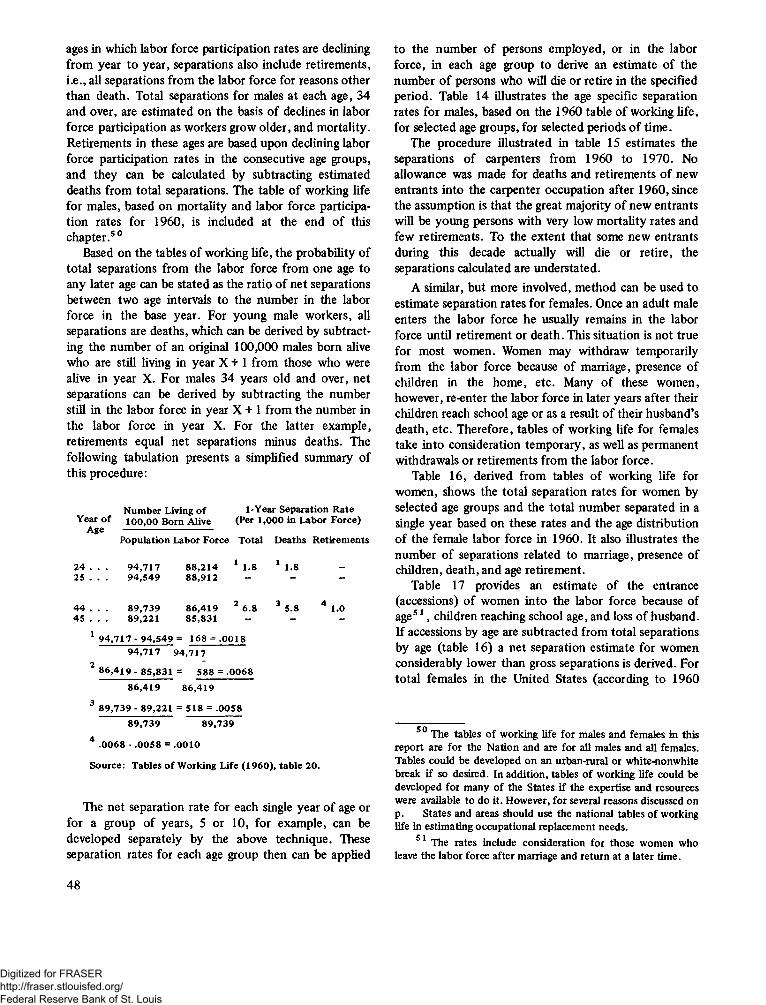
ages in which labor force participation rates are declining from year to year, separations also include retirements, i.e., all separations from the labor force for reasons other than death. Total separations for males at each age, 34 and over, are estimated on the basis of declines in labor force participation as workers grow older, and mortality. Retirements in these ages are based upon declining labor force participation rates in the consecutive age groups, and they can be calculated by subtracting estimated deaths from total separations. The table of working life for males, based on mortality and labor force participation rates for 1960, is included at the end of this chapter.5 0
Based on the tables of working life, the probability of total separations from the labor force from one age to any later age can be stated as the ratio of net separations between two age intervals to the number in the labor force in the base year. For young male workers, all separations are deaths, which can be derived by subtracting the number of an original 100,000 males born alive who are still living in year X + 1 from those who were alive in year X. For males 34 years old and over, net separations can be derived by subtracting the number still in the labor force in year X + 1 from the number in the labor force in year X. For the latter example, retirements equal net separations minus deaths. The following tabulation presents a simplified summary of this procedure:
N um ber Living o f 1-Year Separation R ateYear o f 100,00 Born Alive (Per 1,000 in Labor Force)Age ----------------------------
Population Labor Force Total Deaths R etirem ents
24 . . . 94,717 88,214 1 1.825 . . . 94,549 88,912
44 . . . 89,739 86,419 2 6.845 . . . 89,221 85,831
1 94,717 - 94,549 = 168 = .001894,717 94,717
2 8 6 ,4 1 9 -8 5 ,8 3 1 = 588 = .006886,419 86,419
3 89,739 - 89,221 = 518 = .0058 89,739 89,739
4 .0068 - .0 0 5 8 = .0010
1 1.8
3 5.8 4 1.0
Source: Tables o f Working Life (1960), table 20.
The net separation rate for each single year of age or for a group of years, 5 or 10, for example, can be developed separately by the above technique. These separation rates for each age group then can be applied
to the number of persons employed, or in the labor force, in each age group to derive an estimate of the number of persons who will die or retire in the specified period. Table 14 illustrates the age specific separation rates for males, based on the 1960 table of working life, for selected age groups, for selected periods of time.
The procedure illustrated in table 15 estimates the separations of carpenters from 1960 to 1970. No allowance was made for deaths and retirements of new entrants into the carpenter occupation after 1960, since the assumption is that the great majority of new entrants will be young persons with very low mortality rates and few retirements. To the extent that some new entrants during this decade actually will die or retire, the separations calculated are understated.
A similar, but more involved, method can be used to estimate separation rates for females. Once an adult male enters the labor force he usually remains in the labor force until retirement or death. This situation is not true for most women. Women may withdraw temporarily from the labor force because of marriage, presence of children in the home, etc. Many of these women, however, re-enter the labor force in later years after their children reach school age or as a result of their husband’s death, etc. Therefore, tables of working life for females take into consideration temporary, as well as permanent withdrawals or retirements from the labor force.
Table 16, derived from tables of working life for women, shows the total separation rates for women by selected age groups and the total number separated in a single year based on these rates and the age distribution of the female labor force in 1960. It also illustrates the number of separations related to marriage, presence of children, death, and age retirement.
Table 17 provides an estimate of the entrance (accessions) of women into the labor force because of age51, children reaching school age, and loss of husband. If accessions by age are subtracted from total separations by age (table 16) a net separation estimate for women considerably lower than gross separations is derived. For total females in the United States (according to 1960
50 The tables o f working life for males and fem ales in this report are for the N ation and are for all males and all fem ales. Tables could be developed on an urban-rural or w hite-nonw hite break i f so desired. In addition, tables o f working life could be developed for m any o f the States i f the expertise and resources were available to do it. However, for several reasons discussed on p . States and areas should use the national tables o f working life in estim ating occupational replacem ent needs.
51 The rates include consideration for those w om en w ho leave the labor force after marriage and return at a later tim e.
48
Digitized for FRASER http://fraser.stlouisfed.org/ Federal Reserve Bank of St. Louis
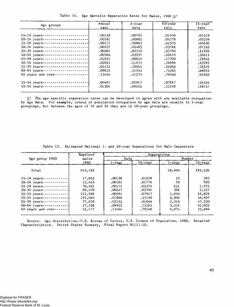
T a b le 1 4 . A ge S p e c i f i c S e p a r a t i o n R a t e s f o r M a l e s , I 9 6 0 1 /
A ge g r o u p s A n n u a lr a t e
5 - y e a rr a t e
1 0 - y e a rr a t e
1 5 - y e a rr a t e
1 4 - 1 9 y e a r s ----------------------------------------------- .0 0 1 2 8 .0 0 7 6 2 .0 1 6 3 9 .0 2 5 1 92 0 - 2 4 y e a r s ----------------------------------------------- .0 0 1 8 1 .0 0 8 8 2 .0 1 7 7 8 .0 3 2 3 62 5 - 2 9 y e a r s ----------------------------------------------- .0 0 1 7 1 .0 0 9 0 3 .0 2 3 7 5 .0 4 6 3 03 0 - 3 4 y e a r s --------------------------------------------- - .0 0 2 2 7 .0 1 4 & 5 .0 3 7 6 1 .0 7 1 6 53 5 - 3 9 y e a r s ----------------------------------------------- .0 0 4 0 1 .0 2 3 1 0 .0 5 7 6 6 .1 2 1 9 64 0 - 4 4 y e a r s ----------------------------------------------- .0 0 5 8 4 .0 3 5 3 7 .1 0 1 1 9 .2 0 6 1 14 5 - 4 9 y e a r s ----------------------------------------------- .0 1 0 3 1 .0 6 8 2 4 .1 7 7 0 0 .3 3 8 4 25 0 - 5 4 y e a r s ----------- ------------------------------------ .0 2 0 1 2 .1 1 6 7 3 .2 8 9 9 8 .6 5 5 9 35 5 - 5 9 y e a r s ----------------------------------------------- .0 3 2 3 2 .1 9 6 1 4 .6 1 0 4 6 .7 8 5 2 56 0 - 6 4 y e a r s ------- ---------------------------------------- .0 9 6 2 5 .5 1 5 4 2 .7 3 2 8 5 .8 6 9 5 265 y e a r s an d o v e r ----------------------------------- 0 1 3 4 6 4 .5 1 2 7 3 .7 9 5 4 0 .9 3 3 4 6
3 5 - 4 4 y e a r s ----------------------------------------------- .0 0 4 9 1 .0 2 9 1 7 .0 7 9 1 7 .1 6 3 5 44 5 - 5 4 y e a r s ----------------------------------------------- .0 1 5 0 4 .0 9 1 6 2 .2 3 1 4 9 .4 9 1 5 7
1 / T he a g e s p e c i f i c s e p a r a t i o n r a t e s c a n b e d e v e l o p e d t o a g r e e w i t h a n y a v a i l a b l e o c c u p a t i o n by a g e d a t a . F o r e x a m p le , c e n s u s o f p o p u l a t i o n o c c u p a t i o n by a g e d a t a a r e u s u a l l y i n 5 - y e a r g r o u p i n g s , b u t b e tw e e n t h e a g e s o f 35 an d 5 4 t h e y a r e i n 1 0 - y e a r g r o u p i n g s .
T a b le 1 5 . E s t im a t e d N a t i o n a l 1 - an d 1 0 - y e a r S e p a r a t i o n s f o r M a le C a r p e n t e r s
A ge g r o u p 1 9 6 0E m p lo y e d
m a le s I 9 6 0
S e p a r a t i o n sR a t e Num ber
1 - y e a r 1 0 - y e a r 1 - y e a r 1 0 - y e a r
T o t a l 8 1 6 , 1 9 5 1 8 ,4 0 4 1 9 3 , 2 2 0
1 4 - 1 9 y e a r s -------------------------- 1 7 ,8 4 2 .0 0 1 2 8 .0 1 6 3 9 23 2 9 22 0 - 2 4 y e a r s -------------------------- 5 3 ,4 1 6 .0 0 1 8 1 .0 1 7 7 8 9 5 9 5 02 5 - 2 9 y e a r s -------------------------- 7 0 ,4 8 1 .0 0 1 7 1 .0 2 3 7 4 121 1 , 6 7 43 0 - 3 4 y e a r s -------------------------- 8 8 ,4 7 0 .0 0 2 2 7 .0 3 7 6 1 201 3 , 3 2 73 5 - 4 4 y e a r s -------------------------- 2 1 2 ,5 6 8 .0 0 4 9 1 .0 7 9 1 7 1 , 0 4 4 1 6 ,8 2 94 5 - 5 4 y e a r s -------------------------- 1 9 3 , 0 8 4 .0 1 5 0 4 .2 3 1 4 9 2 , 9 0 4 4 4 ,6 9 75 5 - 5 9 y e a r s -------------------------- 7 7 ,8 5 9 .0 3 2 3 2 .6 1 0 4 6 2 , 5 1 6 4 7 ,5 3 06 0 - 6 4 y e a r s -------------------------- 5 7 ,3 5 8 .0 9 6 2 5 .7 3 2 8 5 5 ,5 2 1 4 2 ,0 3 565 y e a r s an d o v e r ------------- 4 5 ,1 1 7
<------------------------------------.1 3 4 6 4 .7 9 5 4 0 6 , 0 7 4 3 5 ,8 8 6
S o u r c e : A ge d i s t r i b u t i o n - - U . S . B u r e a u o f C e n s u s , U .S . C e n s u s o f P o p u l a t i o n , 1 9 6 0 . D e t a i l e dC h a r a c t e r i s t i c s . U n i t e d S t a t e s Sum m ary, F i n a l R e p o r t P C ( 1 ) - 1 D .
49
Digitized for FRASER http://fraser.stlouisfed.org/ Federal Reserve Bank of St. Louis
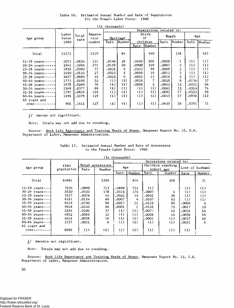
T a b le 1 6 . E s t im a t e d A n n u a l Number and R a te o f S e p a r a t i o n s f o r t h e F e m a le L a b o r F o r c e : 1 9 6 0
( I n t h o u s a n d s )
A ge g r o u pL a b o rf o r c e
1 9 6 0T o t a l
r a t eS e p a r a
t i o nnum ber
S e p a r a t i o n s r e l a t e d t o :
M a r r ia g eB i r t h
o f D e a th A geR a te Number c h i l d r e n R a te Number R a te Number
R a te Number
T o t a l 2 3 2 7 2 1 1 1 9 8 4 4 4 0 138 4 5 7
1 4 - 1 9 y e a r s ----------- 2 0 7 3 .0 6 3 4 131 .0 1 4 0 29 .0 4 8 8 101 .0 0 0 6 1 ( 1 ) ( 1 )2 0 - 2 4 y e a r s ----------- 2 5 4 2 o 1 0 6 6 271 .0 1 5 9 4 0 .0 9 0 0 229 .0 0 0 7 2 ( 1 ) ( 1 )2 5 - 2 9 y e a r s ----------- 19 5 5 .0 3 9 3 77 .0 0 3 1 6 .0 3 5 3 69 .0 0 0 9 2 ( 1 ) ( 1 )3 0 - 3 4 y e a r s ----------- 2 1 8 0 .0 1 2 2 27 .0 0 2 2 5 .0 0 8 8 19 .0 0 1 2 3 ( 1 ) ( 1 )3 5 - 3 9 y e a r s ----------- 2 6 2 7 .0 0 8 4 22 .0 0 1 5 4 .0 0 5 1 13 .0 0 1 8 5 ( 1 ) ( 1 )4 0 - 4 4 y e a r s ----------- 2 7 7 3 .0 1 8 8 52 ( 1 ) ( 1 ) .0 0 2 6 7 .0 0 2 8 8 .0 1 3 4 374 5 - 4 9 y e a r s ----------- 2 8 7 9 .0 2 6 9 78 ( 1 ) ( 1 ) .0 0 0 6 2 .0 0 4 2 12 .0 2 2 1 645 0 - 5 4 y e a r s ----------- 2 3 4 9 .0 3 7 7 89 ( 1 ) ( 1 ) ( 1 ) ( 1 ) .0 0 6 3 15 .0 3 1 4 745 5 - 5 9 y e a r s ----------- 1 7 9 7 .0 6 4 5 11 6 ( 1 ) ( 1 ) ( 1 ) ( 1 ) .0 0 9 2 17 .0 5 5 3 996 0 - 6 4 y e a r s ----------- 1 1 9 6 .1 0 7 9 129 ( 1 ) ( 1 ) ( 1 ) ( 1 ) .0 1 4 3 17 .0 9 3 6 11265 y e a r s and
o v e r --------------------- 90 1 .1 4 1 1 127 ( 1 ) ( 1 ) ( 1 ) ( 1 ) .0 6 3 0 56 .0 7 8 1 71
1 / Am ount n o t s i g n i f i c a n t .
N o t e : T o t a l s may n o t add d u e t o r o u n d in g .
S o u r c e : Work L i f e E x p e c ta n c y and T r a i n in g N e e d s o f Women, M anpower R e p o r t N o. 1 2 . U .S .D e p a r tm e n t o f L a b o r , M anpower A d m i n i s t r a t i o n .
T a b le 1 7 . E s t im a t e d A n n u a l Number and R a te o f A c c e s s i o n s t o t h e F e m a le L a b o r F o r c e : 1 9 6 0
( I n t h o u s a n d s )
A ge g r o u p 1 9 6 0p o p u l a t i o n
T o t a l a c c e s s i o n sA c c e s s i o n s r e l a t e d t o :
A ge C h i ld r e n r e a c h in g s c h o o l a g e L o s s o f h u sb a n dR a te Number
R a te Number R a te Number R a te NumberT o t a l 6 4 9 6 1 1 2 9 6 9 1 6 3 0 9 71
1 4 - 1 9 y e a r s ------- 7 9 3 4 .0 8 9 8 7 1 2 .0 8 9 8 71 2 ( 1 ) ( 1 ) ( 1 )2 0 - 2 4 y e a r s ------- 5 5 2 0 .0 3 2 3 178 .0 3 1 6 1 7 4 .0 0 0 7 4 ( 1 ) ( 1 )2 5 - 2 9 y e a r s ------- 5 5 3 7 .0 0 7 6 42 .0 0 2 5 14 .0 0 5 1 28 ( 1 ) ( 1 )3 0 - 3 4 y e a r s ------- 61 1 1 .0 1 1 4 69 .0 0 0 7 4 .0 1 0 7 65 ( 1 ) ( 1 )3 5 - 3 9 y e a r s ------- 6 4 1 9 .0 1 5 0 96 .0 0 1 7 11 .0 1 2 5 8 0 .0 0 0 8 54 0 - 4 4 y e a r s ------- 5 9 1 8 .0 1 4 4 86 .0 0 0 1 1 .0 1 2 6 75 .0 0 1 7 104 5 - 4 9 y e a r s ------- 5 5 5 4 .0 1 0 2 57 ( 1 ) ( 1 ) .0 0 7 7 43 .0 0 2 5 145 0 - 5 4 y e a r s ------- 4 9 3 2 .0 0 6 4 32 ( 1 ) ( 1 ) .0 0 2 8 14 .0 0 3 6 185 5 - 5 9 y e a r s ------- 4 4 1 1 .0 0 3 8 16 ( 1 ) ( 1 ) .0 0 0 1 ( 1 ) .0 0 3 7 166 0 - 6 4 y e a r s ------- 3 7 2 7 .0 0 2 1 8 ( 1 ) ( 1 ) ( 1 ) ( 1 ) .0 0 2 1 865 y e a r s and
o v e r ----------------- 8 8 9 8 ( 1 ) ( 1 ) ( 1 )j
( 1 ) ( 1 ) ( 1 ) ( 1 )
IV A m ounts n o t s i g n i f i c a n t .
N o t e : T o t a l s may n o t add d u e t o r o u n d in g .
S o u r c e : Work L i f e E x p e c ta n c y and T r a in in g N e e d s o f Women, M anpower R e p o r t N o. 1 2 , U .S .D e p a r tm e n t o f L a b o r , M anpower A d m i n i s t r a t i o n .
50
Digitized for FRASER http://fraser.stlouisfed.org/ Federal Reserve Bank of St. Louis
information) the total gross separation rate for females would be about 4.8 percent, compared with a net separation rate of about 3.2 percent.52
To estimate gross separations for females in a particular occupation, the age specific total separation rates found in table 16 would be applied to the number of workers in each age group. Table 18 illustrates a calculation of the annual gross separations for secretaries, stenographers, and typists—110,758 (or 5.1 percent of the total). If training needs were being calculated instead of manpower requirements, gross separations could be reduced to the extent that qualified secretaries return from outside the labor force by applying the accession rates in table 17 to the approximate age groups, and subtracting the resultant from gross separations.53
Separation rates for females have been developed for 1 year only (see tables 16 and 17), due to the characteristics of the participation of females in the labor force. Occupational replacement needs for females for 5, 10, or 15 year age groups can be approximated by multiplying the 1-year rates by the respective number of years; the assumption is that new entrants into the occupation will maintain the 1960 age distribution.
52Gross
Separations m inus (thousands)
Accessions equals (thousands)
N etSeparations(thousands)
84 (marriage) 71 Goss o fhusband)
13
4 4 0 (birth o f children)
309 (children reaching school age)
131
595 (deaths andretirem ents)
1119 Total 3 8 0 Total 73 9 Total
The tota l separation rate for fem ales is com puted as follow s: to ta l num ber o f separations 1 ,119 = .0481total labor force 2 3 ,2 7 2
The net separation rate is com puted as follow s:net num ber o f separations 73 9 = .031 8total labor force 2 3 ,2 7 2
53 From a training point o f view , how ever, w om en w ho have been ou t o f the labor force for several years may need significant refresher training before taking over the duties o f an occupation at w hich they were em ployed 10 to 15 years before. M oreover, this adjustm ent assum es that fem ale secretaries, stenographers, and typists have the same temporary retirem ent patterns as fem ale workers as a w hole.
LimitationsSeveral assumptions underlie the development and
use of separation rates. One significant assumption is that mortality trends and retirement patterns do not differ by occupation. This statement is not true, however. Differences in the nature of work, the exposure of workers to disabilizing work environments, the coverage and provision of pension plans, the extent of opportunities for employment, and many other factors influence retirement patterns and mortality trends among occupations. For example, the retirement pattern of physicians, who often practice until old age, is very different from that of linemen or roofers, who withdraw from these occupations at a young age because of the physical requirements of these jobs. Similarly, the use of overall separation rates for women assumes that the characteristics of marriage, presence of children in the home, etc., have the same affect on all females regardless of occupation. Women who have the greatest amount of education and, thus, who are concentrated in certain occupations, however, have higher labor force participation rates than the average. Their temporary withdrawal from the labor force, therefore, is much less certain than for women with less education.
The national separation rates are given in appendix A to this volume. For several occupations, the number of separations derived by using these rates has been compared with data from other sources. For example, for several skilled building trades, the U.S. Department of Labor has collected statistics on the number of journeymen per 1,000 who become unavailable for work because of death, permanent disability, or retirement during a 12-month period. In general, the average rates based on these surveys were very similar to the computed death and retirement rates derived by using tables of working life. Rates for metal trades occupations developed in a 1957 study of the New York State Department of Labor were very similar to those computed by the methods described in this chapter.54 On the basis of these evaluations, these rates are quite representative of the true rates for most occupations. In the absence of more comprehensive data for individual occupations, the tables of working life provide a systematic method for obtaining an estimate of the general magnitude of separations resulting from deaths and retirements. Regional analysts, however, should
54 M an pow er in S e le c ted M eta l Crafts, N e w Y ork S ta te , N ew York State Departm ent o f Labor, Division o f Research and Statistics, Publication N o. R -1 0 7 ,1 9 59 .
51
Digitized for FRASER http://fraser.stlouisfed.org/ Federal Reserve Bank of St. Louis
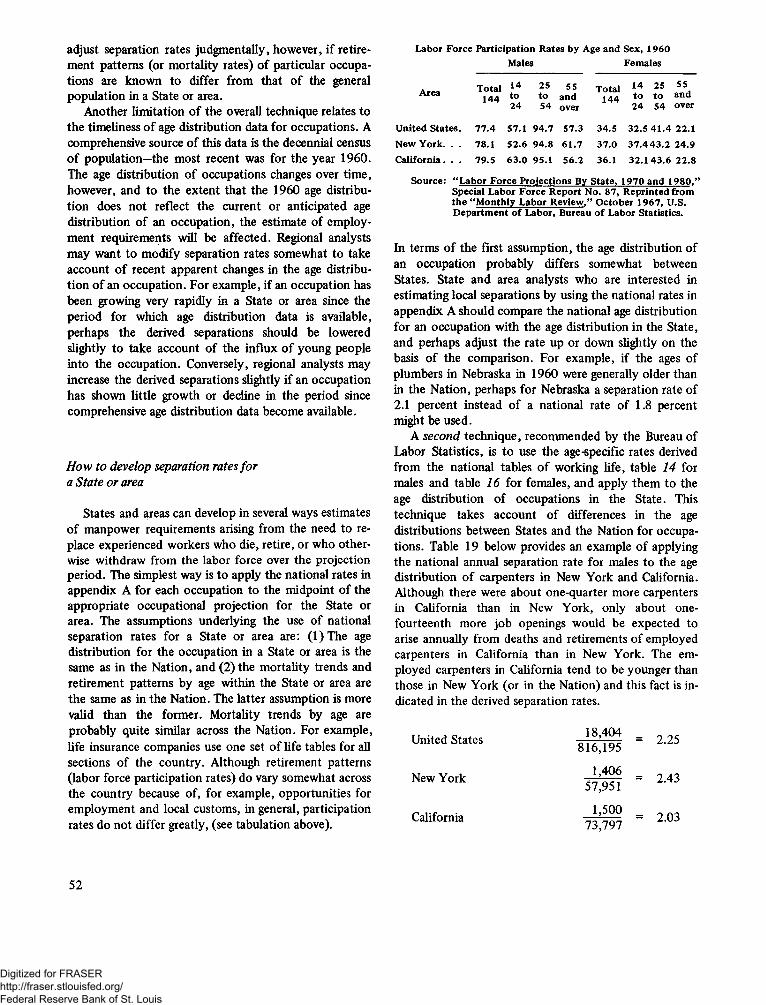
adjust separation rates judgmentally, however, if retirement patterns (or mortality rates) of particular occupations are known to differ from that of the general population in a State or area.
Another limitation of the overall technique relates to the timeliness of age distribution data for occupations. A comprehensive source of this data is the decennial census of population—the most recent was for the year 1960. The age distribution of occupations changes over time, however, and to the extent that the 1960 age distribution does not reflect the current or anticipated age distribution of an occupation, the estimate of employment requirements will be affected. Regional analysts may want to modify separation rates somewhat to take account of recent apparent changes in the age distribution of an occupation. For example, if an occupation has been growing very rapidly in a State or area since the period for which age distribution data is available, perhaps the derived separations should be lowered slightly to take account of the influx of young people into the occupation. Conversely, regional analysts may increase the derived separations slightly if an occupation has shown little growth or decline in the period since comprehensive age distribution data become available.
How to develop separation rates for a State or area
States and areas can develop in several ways estimates of manpower requirements arising from the need to replace experienced workers who die, retire, or who otherwise withdraw from the labor force over the projection period. The simplest way is to apply the national rates in appendix A for each occupation to the midpoint of the appropriate occupational projection for the State or area. The assumptions underlying the use of national separation rates for a State or area are: (l)The age distribution for the occupation in a State or area is the same as in the Nation, and (2) the mortality trends and retirement patterns by age within the State or area are the same as in the Nation. The latter assumption is more valid than the former. Mortality trends by age are probably quite similar across the Nation. For example, life insurance companies use one set of life tables for all sections of the country. Although retirement patterns (labor force participation rates) do vary somewhat across the country because of, for example, opportunities for employment and local customs, in general, participation rates do not differ greatly, (see tabulation above).
Labor Force Participation Rates by Age and Sex, 1960 Males Females
Area Total144
14to24
25to54
55andover
T otal144
14 25 55 to to and 24 54 over
U nited S tates. 77.4 57.1 94.7 57.3 34.5 32.5 41.4 22.1New Y ork. . . 78.1 52.6 94.8 61.7 37.0 37 .443.2 24.9C alifornia. . . 79.5 63.0 95.1 56.2 36.1 32 .143 .6 22.8
Source: “ Labor Force Projections By S tate, 1970 and 1980.” Special Labor Force R eport No. 87, R eprinted from th e “ M onthly L abor Review,” O ctober 1967, U.S. D epartm ent o f Labor, Bureau o f Labor Statistics.
In terms of the first assumption, the age distribution of an occupation probably differs somewhat between States. State and area analysts who are interested in estimating local separations by using the national rates in appendix A should compare the national age distribution for an occupation with the age distribution in the State, and perhaps adjust the rate up or down slightly on the basis of the comparison. For example, if the ages of plumbers in Nebraska in 1960 were generally older than in the Nation, perhaps for Nebraska a separation rate of2.1 percent instead of a national rate of 1.8 percent might be used.
A second technique, recommended by the Bureau of Labor Statistics, is to use the age-specific rates derived from the national tables of working life, table 14 for males and table 16 for females, and apply them to the age distribution of occupations in the State. This technique takes account of differences in the age distributions between States and the Nation for occupations. Table 19 below provides an example of applying the national annual separation rate for males to the age distribution of carpenters in New York and California. Although there were about one-quarter more carpenters in California than in New York, only about one- fourteenth more job openings would be expected to arise annually from deaths and retirements of employed carpenters in California than in New York. The employed carpenters in California tend to be younger than those in New York (or in the Nation) and this fact is indicated in the derived separation rates.
United States 18,404 = 2.25816,195New York 1,406 = 2.4357,951California 1,500
73,797 = 2.03
52
Digitized for FRASER http://fraser.stlouisfed.org/ Federal Reserve Bank of St. Louis
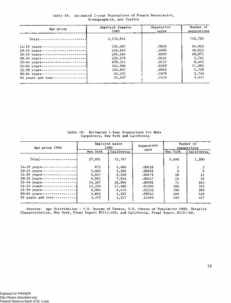
T a b l e 1 8 . E s t i m a t e d 1 - y e a r S e p a r a t i o n s o f F e m a l e S e c r e t a r i e s S t e n o g r a p h e r s , a n d T y p i s t s
A g e g r o u p E m p l o y e d f e m a l e s 1 9 6 0
S e p a r a t i o nr a t e s
N u m b e r o f s e p a r a t i o n s
T o t a l ............................................. ....................... 2 , 1 7 8 , 6 4 1 1 1 0 , 7 5 8
1 4 - 1 9 y e a r s ------------------------------------------------------------------ 2 3 5 , 4 0 7 . 0 6 3 4 1 4 , 9 2 52 0 - 2 4 y e a r s ------------------------------------------------------------------ 4 5 6 , 1 4 0 . 1 0 6 6 4 8 , 6 2 52 5 - 2 9 y e a r s --------------------------------------------------- -------------- 2 5 6 , 2 6 4 . 0 3 9 3 1 0 , 0 7 13 0 - 3 4 y e a r s ---------------------- -------------------- ----------------------- 2 2 6 , 2 7 8 . 0 1 2 2 2 , 7 6 13 5 - 4 4 y e a r s ------------------------------------------------------------------ 4 7 0 , 3 1 1 . 0 1 3 7 6 , 4 4 34 5 - 5 4 y e a r s ------------------------------------------------------------------ 3 4 4 , 9 0 0 . 0 3 1 9 1 1 , 0 0 25 5 - 5 9 y e a r s ------------------------------------------------------------------- 1 0 4 , 6 5 7 . 0 6 4 5 6 , 7 5 06 0 - 6 4 y e a r s ------------------------------------------------------------------ 5 3 , 2 3 7 . 1 0 7 9 5 , 7 4 46 5 y e a r s a n d o v e r ------------------------------------------------ 3 1 , 4 4 7 . 1 4 1 1
14 , 4 3 7
T a b l e 1 9 . E s t i m a t e d 1 - Y e a r C a r p e n t e r s , New Y o r k
S e p a r a t i o n s f o r M a l e a n d C a l i f o r n i a
A g e g r o u p 1 9 6 0E m p l o y e d m a l e s
1 9 6 0 S e p a r a t i o n N u m b e r o f s e p a r a t i o n s
New Y o r k C a l i f o r n i ar a t e
New Y o r k C a l i f o r n i a
T o t a l ------------- -------------------- -------------------- 5 7 , 9 5 1 7 3 , 7 9 7 1 , 4 0 6 1 , 5 0 0
1 4 - 1 9 y e a r s --------------------------------------------------- 8 7 2 1 , 4 0 6 . 0 0 1 2 8 1 22 0 - 2 4 y e a r s --------------------------------------------------- 3 , 4 8 4 5 , 2 0 4 . 0 0 1 8 1 6 92 5 - 2 9 y e a r s --------------------------------------------------- 5 , 6 2 7 6 , 5 3 6 . 0 0 1 7 1 1 0 113 0 - 3 4 y e a r s --------------------------------------------------- 6 , 9 6 1 7 , 9 2 5 . 0 0 2 2 7 16 1 83 5 - 4 4 y e a r s --------------------------------------------------- 1 4 , 3 8 7 2 0 , 9 0 4 . 0 0 4 9 1 7 1 1 0 34 5 - 5 4 y e a r s ------------- -------------- ----------------------- 1 2 , 3 3 8 1 7 , 4 8 0 . 0 1 5 0 4 1 8 6 2 6 35 5 - 5 9 y e a r s --------------------------------------------------- 6 , 0 6 4 6 , 4 7 4 . 0 3 2 3 2 1 9 6 2 0 96 0 - 6 4 y e a r s --------------------------------------------------- 4 , 8 4 3 4 , 5 5 1 . 0 9 6 2 5 4 6 6 4 3 86 5 y e a r s a n d o v e r --------------------------------- 3 , 3 7 5 3 , 3 1 7 . 1 3 4 6 4 4 5 4 4 4 7
S o u r c e s : A g eC h a r a c t e r i s t i c s ,
d i s t r i b u t i o n - U . S . B u r e a u o f C e n s u s , U . S . C e n s u s New Y o r k , F i n a l R e p o r t P C ( 1 ) - 3 4 D , a n d C a l i f o r n i a ,
o f P o p u l a t i o n 1 9 6 0 , D e t a i l e d F i n a l R e p o r t P C ( 1 ) - 6 D .
53
Digitized for FRASER http://fraser.stlouisfed.org/ Federal Reserve Bank of St. Louis
States and areas that have the time, the resources, the expertise, and the data sources can develop their own tables of working life. From these tables, age specific separation rates can be computed similar to those developed by BLS for the Nation and described above. This technique is involved technically and the derived rates for States probably would not add the degree of precision to the estimate of manpower requirements worth the expenditure of time and resources. Nevertheless, decisions about such computations should be made by the respective State or area analysts who are familiar with local data sources and the technical and financial resources available.
Transfers to Other Occupations
Transfer from one occupation to another occupation is an additional factor that can be considered when estimates of future manpower or training requirements are being developed. In some occupations, the transfer rate may be as high as the death and retirement rate.
In general, workers tend to move from less skilled to more skilled occupations. For example, a factory operator may become a foreman, and move from a semiskilled to a skilled classification; similarly, a mechanic may transfer to a technician job, and shift from the craftsmen to the professional, technical, and kindred workers classification. This type of transfer is usually the result of long experience, often supplemented by additional training.
Unfortunately, comprehensive data are not available on the rate of transfers between occupations. Most of the data available stems from selected sample studies of work histories collected from individuals. One such study, Postcensal S tudy o f Professional and Technical Personnel, followed up 2 years after the 1960 census persons classified in science, engineering, and other professional and technical occupations. The purpose of the study was to determine the proportion of workers who changed occupations over the 2-year period. For example, the annual transfer rate for engineers was estimated at 1.6 percent, for life scientists, 2.6 percent, for technicians, 3 percent.
Another study, Career Patterns o f Former Apprentices, (U.S. Department of Labor, Bulletin T-147, March 1959), provides information on occupational transfers for several craft occupations. For example, more than 10 percent of the apprentice carpenters who completed the apprenticeship program in 1950 were in other occupations in 1956. Moreover, estimates of losses to teaching occupations have been developed from surveys prepared
by the U.S. Office of Education. Two detailed studies of teacher turnover (1957-58 and 1959-60) determined the number of teachers who left their positions between the beginning of one school year and the next.55 The separation rate for elementary school teachers based on this study was 8.1 percent. About one-half of these separations were deaths and withdrawals from the labor force, and the remainder were transfers to other occupations.
A monumental study5 6 of mobility was made by the Social Science Research Council. Ten-year work histories were collected from workers in sample households in each of 6 large cities. In all, 13,000 work history schedules were collected. Each job held by the workers were classified by occupation and occupation group. Thus, for each person, one could obtain the number of job changes and occupational changes made. By combining the data, a measure of the incidence and the pattern of movement out of an occupation was obtained.
Several other attempts have been made to measure the rate of movement out of an occupation. Two studies analyzed net occupational mobility57 by applying cohort analysis to the data from successive censuses of population supplemented by the monthly labor force survey.58 “Model Cohort Work Experience Tables” were designed for major occupational groups. The primary purpose of the study was to determine (1) the net
55 Teacher Turnover in the Public Schools, 1957-58, U.S. Office of Education, OE-23002, Circular 608,1959, and Teacher Turnover in Public Elementary and Secondary Schools, 1959-60, OE-23002-60, Circular 675,1963.
56 Gladys L. Palmer, Labor Mobility in 6 Cities, New York, Social Science Research Council, 1954.
57 “A Note on Occupational Mobility for White and Nonwhite Males, 1950 to 1965,” A. J. Jaffe and J. B. Gordon, The N ew York Statistician , December 1966. This study defines net mobility as the following: “The estimates of net occupational movement were derived by following an age cohort of men from one census period to another. For example, let us suppose that there were 1,000 men aged 30 to 34 years in service occupations in 1950. By 1960 these men were aged 40 to 44. Let us assume that 50 of these men have died, leaving 950 alive. If we find that the 1960 census reports 1,100 men in service occupations aged 40 to 44, we assume that there was a net in-movement of 150 men into this occupation group (1,100-950= 150).”
58 “Occupational Mobility in the United States,” A. J. Jaffe and R. O. Carleton, New York, King Crown Press, 1954 and “A Note on Occupational Mobility for White and Nonwhite Males, 1950 to 1965,” A. J. Jaffe and J. B. Gordon, The N ew York Statistician, December 1966.
54
Digitized for FRASER http://fraser.stlouisfed.org/ Federal Reserve Bank of St. Louis
occupational mobility that actually occurred; (2) the occupational distribution of new entrances into the labor force; and (3) the occupational distribution of retirements from the labor force. The net mobility estimate was the difference between the number of persons moving into and out of an occupation. Recently, work has proceeded on a white-non white break between 1950 and 1965.
Recently, the Bureau of Labor Statistics undertook a study of occupational mobility. This study adds to an earlier one made on the shifts of workers from one employer to another during 1961 that yielded some valuable insights into the mobility of men and women by age and occupational group. The new study focuses on the occupational shifts of workers in major occupational groups between January 1965 and January 1966.59
Although little comprehensive data is available to estimate changes in occupational requirements due to transfers between occupations, this weakness in the technique is not considered greatly significant for the planning of education and training programs. Generally,
59 “Occupational M obility o f E m ployed Workers,** Special Labor Force R ep ort No. 84 reprinted from the M onthly Labor R eview , June 1967, U.S. Department of Labor, Bureau of Labor Statistics.
estimates of occupational requirements based on expected growth and replacements are adequate for most planning purposes. Most States or areas do not have the available resources to train workers to fill all the anticipated job openings in occupations. Moreover, to do so probably would be wasteful because many workers pick up an occupation informally, for example, and learn by observing or working at various aspects of a trade until most or all have been learned. Indications are that many workers have learned the skills of their trade informally.60 The fact that workers are not trained to fill all anticipated job openings provides some flexibility in the future supply of workers to be filled by the transfer of workers between occupations. There are other ways also by which employers can overcome a shortage of skills. Depending upon the extent of under supply in an occupation, local employers will tend to find ways to “make do” with the available skills through, for example, in plant education, job redesign and the use of job aides, general upgrading, reorganization of work, and hiring outside the geographic area.
60 See, Formal Occupational Training o f A d u lt Workers, Manpower Automation Research Monograph No. 2, U.S. Department of Labor, Manpower Administration, Office of Manpower, Automation and Training, December 1964.
55
Digitized for FRASER http://fraser.stlouisfed.org/ Federal Reserve Bank of St. Louis
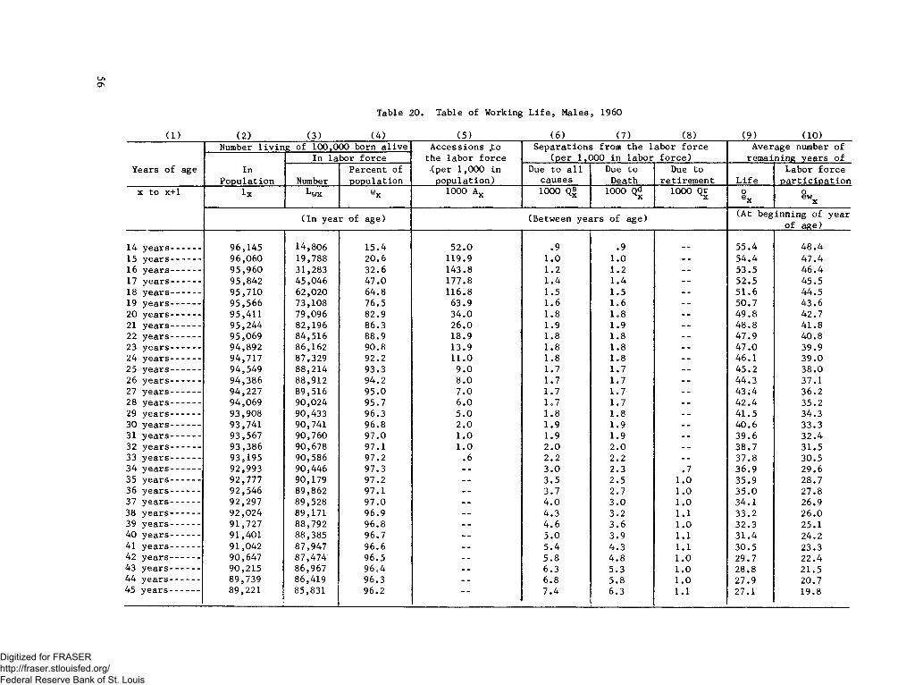
LnOs
T a b l e 2 0 . T a b l e o f W o r k i n g L i f e , M a l e s , 1 9 6 0
( 1 )
Y e a r s o f
x t o x +1
1 4 y e a r s - -15 y e a r s - -16 y e a r s - -17 y e a r s - -18 y e a r s - -19 y e a r s - -2 0 y e a r s - -21 y e a r s - -22 y e a r s - -23 y e a r s - -2 4 y e a r s - -2 5 y e a r s - -2 6 y e a r s - -27 y e a r s - -2 8 y e a r s - -2 9 y e a r s - -3 0 y e a r s - -31 y e a r s - -3 2 y e a r s - -3 3 y e a r s - -3 4 y e a r s - -3 5 y e a r s - -3 6 y e a r s - -3 7 y e a r s - -3 8 y e a r . s - -39 y e a r s - -4 0 y e a r s - -41 y e a r s - -4 2 y e a r s - -4 3 y e a r s - -4 4 y e a r s - -4 5 y e a r s - -
( 2 ) ( 3 ) ( 4 ) ( 5 ) ( 6 ) ( 7 ) ( 8 ) ( 9 ) ( 1 0 )Num ber l i v i n g o f 1 0 0 , 0 0 0 b o r n a l i v e A c c e s s i o n s .to S e p a r a t i o n s f r o m t h e l a b o r f o r c e A v e r a g e n u m b e r o f
I n l a b o r f o r c e t h e l a b o r f o r c e ( p e r 1 , 0 0 0 i n l a b o r f o r c e ) r e m a i n i n g y e a r s o fI n P e r c e n t o f ( p e r 1 , 0 0 0 i n Due t o a l l Due t o Due t o L a b o r f o r c e
P o p u l a t i o n Number p o p u l a t i o n p o p u l a t i o n ) c a u s e s D e a t h r e t i r e m e n t L i f e p a r t i c i p a t i o n
l x ^w x wx 1 0 0 0 A x 1 0 0 0 QS 1 0 0 0 Qd 1 0 0 0 Q rX
oe x
Od)
( I n y e a r o f a g e ) ( B e t w e e n y e a r s o f a g e ) ( A t b e g i n n i n g o f y e a r o f a g e )
9 6 , 1 4 5 1 4 , 8 0 6 1 5 . 4 5 2 . 0 . 9 . 9 . . 5 5 . 4 4 8 . 49 6 , 0 6 0 1 9 , 7 8 8 2 0 . 6 1 1 9 . 9 1 . 0 1 . 0 - - 5 4 . 4 4 7 . 49 5 , 9 6 0 3 1 , 2 8 3 3 2 . 6 1 4 3 . 8 1 . 2 1 . 2 - - 5 3 . 5 4 6 . 49 5 , 8 4 2 4 5 , 0 4 6 4 7 . 0 1 7 7 . 8 1 . 4 1 . 4 5 2 . 5 4 5 . 59 5 , 7 1 0 6 2 , 0 2 0 6 4 . 8 1 1 6 . 8 1 . 5 1 . 5 5 1 . 6 4 4 . 59 5 , 5 6 6 7 3 , 1 0 8 7 6 . 5 6 3 . 9 1 . 6 1 . 6 - - 5 0 . 7 4 3 . 69 5 , 4 1 1 7 9 , 0 9 6 8 2 . 9 3 4 . 0 1 . 8 1 . 8 - - 4 9 . 8 4 2 . 79 5 , 2 4 4 8 2 , 1 9 6 8 6 . 3 2 6 . 0 1 . 9 1 . 9 - - 4 8 . 8 4 1 . 89 5 , 0 6 9 8 4 , 5 1 6 8 8 . 9 1 8 . 9 1 . 8 1 . 8 - - 4 7 . 9 4 0 . 89 4 , 8 9 2 8 6 , 1 6 2 9 0 . 8 1 3 . 9 1 . 8 1 . 8 - - 4 7 . 0 3 9 . 99 4 , 7 1 7 8 7 , 3 2 9 9 2 . 2 1 1 . 0 1 . 8 1 . 8 - - 4 6 . 1 3 9 . 09 4 , 5 4 9 8 8 , 2 1 4 9 3 . 3 9 . 0 1 . 7 1 . 7 - - 4 5 . 2 3 8 . 09 4 , 3 8 6 8 8 , 9 1 2 9 4 . 2 8 . 0 1 . 7 1 . 7 - - 4 4 . 3 3 7 . 19 4 , 2 2 7 8 9 , 5 1 6 9 5 . 0 7 . 0 1 . 7 1 . 7 - - 43 ; 4 3 6 . 29 4 , 0 6 9 9 0 , 0 2 4 9 5 . 7 6 . 0 1 . 7 1 . 7 - - 4 2 . 4 3 5 . 29 3 , 9 0 8 9 0 , 4 3 3 9 6 . 3 5 . 0 1 . 8 1 . 8 - - 4 1 . 5 3 4 . 39 3 , 7 4 1 9 0 , 7 4 1 9 6 . 8 2 . 0 1 . 9 1 . 9 - - 4 0 . 6 3 3 . 39 3 , 5 6 7 9 0 , 7 6 0 9 7 . 0 1 . 0 1 . 9 1 . 9 - - 3 9 . 6 3 2 . 49 3 , 3 8 6 9 0 , 6 7 8 9 7 . 1 1 . 0 2 . 0 2 . 0 3 8 . 7 3 1 . 59 3 , 1 9 5 9 0 , 5 8 6 9 7 . 2 . 6 2 . 2 2 . 2 3 7 . 8 3 0 . 59 2 , 9 9 3 9 0 , 4 4 6 9 7 . 3 - - 3 . 0 2 . 3 . 7 3 6 . 9 2 9 . 69 2 , 7 7 7 9 0 , 1 7 9 9 7 . 2 - - 3 . 5 2 . 5 1 . 0 3 5 . 9 2 8 . 79 2 , 5 4 6 8 9 , 8 6 2 9 7 . 1 - - 3 . 7 2 . 7 1 . 0 3 5 . 0 2 7 . 89 2 , 2 9 7 8 9 , 5 2 8 9 7 . 0 - - 4 . 0 3 . 0 1 . 0 3 4 . 1 2 6 . 99 2 , 0 2 4 8 9 , 1 7 1 9 6 . 9 - - 4 . 3 3 . 2 1 . 1 3 3 . 2 2 6 . 09 1 , 7 2 7 8 8 , 7 9 2 9 6 . 8 - - 4 . 6 3 . 6 1 . 0 3 2 . 3 2 5 . 19 1 , 4 0 1 8 8 , 3 8 5 9 6 . 7 - - 5 . 0 3 . 9 1 . 1 3 1 . 4 2 4 . 29 1 , 0 4 2 8 7 , 9 4 7 9 6 . 6 - - 5 . 4 4 . 3 1 . 1 3 0 . 5 2 3 . 39 0 , 6 4 7 8 7 , 4 7 4 9 6 . 5 5 . 8 4 . 8 1 . 0 2 9 . 7 2 2 . 49 0 , 2 1 5 8 6 , 9 6 7 9 6 . 4 - - 6 . 3 5 . 3 1 . 0 2 8 . 8 2 1 . 58 9 , 7 3 9 8 6 , 4 1 9 9 6 . 3 - - 6 . 8 5 . 8 1 . 0 2 7 . 9 2 0 . 78 9 , 2 2 1 8 5 , 8 3 1 9 6 . 2 7 . 4 6 . 3 1 . 1 2 7 . 1 1 9 . 8
Digitized for FRASER http://fraser.stlouisfed.org/ Federal Reserve Bank of St. Louis
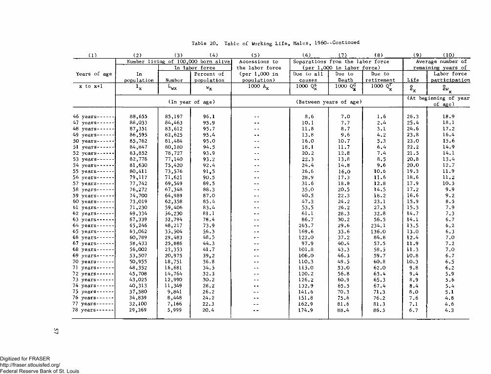
T a b l e 2 0 , T a b l e o f W o r k in g L i f e , M a l e s , 1 9 6 0 - - C o n t i n u e d
( 1 )
Y e a r s o f
x t o x +1
4 6 y e a r s47 y e a r s4 8 y e a r s4 9 y e a r s5 0 y e a r s51 y e a r s5 2 y e a r s53 y e a r s5 4 y e a r s55 y e a r s5 6 y e a r s57 y e a r s5 8 y e a r s5 9 y e a r s6 0 y e a r s61 y e a r s62 y e a r s63 y e a r s6 4 y e a r s65 y e a r s66 y e a r s67 y e a r s6 8 y e a r s69 y e a r s7 0 y e a r s71 y e a r s7 2 y e a r s73 y e a r s7 4 y e a r s -75 y e a r s7 6 y e a r s -77 y e a r s -78 y e a r s -
( 2 ) ( 3 ) ( 4 ) ( 5 ) ( 6 ) ( 7 ) ( 8 ) ( 9 ) ( 1 0 )Num ber l i v i n g o f 1 0 0 , 0 0 0 b o r n a l i v e A c c e s s i o n s t o S e p a r a t i o n s f r o m t h e l a b o r f o r c e A v e r a g e n u m b e r o f
I n l a b o r f o r c e t h e l a b o r f o r c e ( p e r 1 , 0 0 0 i n l a b o r f o r c e ) r e m a i n i n g y e a r s o fI n P e r c e n t o f ( p e r 1 , 0 0 0 i n Due t o a l l Due t o Du e t o L a b o r f o r c e
p o p u l a t i o n Number p o p u l a t i o n p o p u l a t i o n ) c a u s e s D e a t h r e t i r e m e n t L i f e p a r t i c i p a t i o n
^wx wx 1 0 0 0 A x 1 0 0 0 QS 1 0 0 0 Qd 1 0 0 0 Q rX
oe x
oewX
( I n y e a r o f a g e ) ( B e t w e e n y e a r s o f a g e )( A t b e g i n n i n g o f y e a r
o f a g e )
8 8 , 6 5 5 8 5 , 1 9 7 9 6 . 1 8 . 6 7 . 0 1 . 6 2 6 . 3 1 8 . 98 8 , 0 3 3 8 4 , 4 6 3 9 5 . 9 - - 1 0 . 1 7 . 7 2 . 4 2 5 . 4 1 8 . 18 7 , 3 5 1 8 3 , 6 1 2 9 5 . 7 - - 1 1 . 8 8 . 7 3 . 1 2 4 . 6 1 7 . 28 6 , 5 9 5 8 2 , 6 2 5 9 5 . 4 - - 1 3 . 8 9 . 6 4 . 2 2 3 . 8 1 6 . 48 5 , 7 6 2 8 1 , 4 8 4 9 5 . 0 - - 1 6 . 0 1 0 . 7 5 . 3 2 3 . 0 1 5 . 68 4 , 8 4 7 8 0 , 1 8 0 9 4 . 5 - - 1 8 . 1 1 1 . 7 6 . 4 2 2 . 2 1 4 . 98 3 , 8 5 2 7 8 , 7 2 7 9 3 . 9 - - 2 0 . 2 1 2 . 8 7 . 4 2 1 . 5 1 4 . 18 2 , 7 7 8 7 7 , 1 4 0 9 3 . 2 - - 2 2 . 3 1 3 . 8 8 . 5 2 0 . 8 1 3 . 48 1 , 6 3 0 7 5 , 4 2 0 9 2 . 4 - - 2 4 . 4 1 4 . 8 9 . 6 2 0 . 0 1 2 . 78 0 , 4 1 1 7 3 , 5 7 6 9 1 , 5 - - 2 6 . 6 1 6 . 0 1 0 . 6 1 9 . 3 1 1 . 97 9 * 1 1 7 7 1 , 6 2 1 9 0 . 5 - - 2 8 . 9 1 7 . 3 1 1 . 6 1 8 . 6 1 1 . 27 7 , 7 4 2 6 9 , 5 4 9 8 9 . 5 - - 3 1 . 6 1 8 . 8 1 2 . 8 1 7 . 9 1 0 . 57 6 , 2 7 2 6 7 , 3 4 8 8 8 . 3 - - 3 5 . 0 2 0 . 5 1 4 . 5 1 7 . 2 9 . 97 4 , 7 0 0 6 4 , 9 8 9 8 7 . 0 - - 4 0 . 5 2 2 . 3 1 8 . 2 1 6 . 6 9 . 27 3 , 0 1 9 6 2 , 3 5 8 8 5 . 4 - - 4 7 . 3 2 4 . 2 2 3 . 1 1 5 . 9 8 . 57 1 , 2 3 0 5 9 , 4 0 6 8 3 . 4 - - 5 3 . 5 2 6 . 2 2 7 . 3 1 5 . 3 7 . 96 9 , 3 3 4 5 6 , 2 3 0 8 1 . 1 - - 6 1 . 1 2 8 . 3 3 2 . 8 1 4 . 7 7 . 36 7 , 3 3 9 5 2 , 7 9 4 7 8 . 4 - - 8 6 . 7 3 0 . 2 5 6 . 5 1 4 . 1 6 . 76 5 , 2 4 6 4 8 , 2 1 7 7 3 . 9 - - 2 6 3 . 7 2 9 . 6 2 3 4 . 1 1 3 . 5 6 . 26 3 , 0 6 2 3 5 , 5 0 4 5 6 . 3 - - 1 6 9 . 6 3 3 . 6 1 3 6 . 0 1 3 . 0 6 . 36 0 , 7 8 9 2 9 , 4 8 3 4 8 . 5 - - 1 2 2 . 0 3 7 . 2 8 4 . 8 1 2 . 4 7 . 05 8 , 4 3 3 2 5 , 8 8 6 4 4 . 3 - - 9 7 . 9 4 0 . 4 5 7 . 5 1 1 . 9 7 . 25 6 , 0 0 2 2 3 , 3 5 3 4 1 . 7 - - 1 0 1 . 8 4 3 . 3 5 8 . 5 1 1 . 3 7 . 05 3 , 5 0 7 2 0 , 9 7 5 3 9 , 2 - - 1 0 6 . 0 4 6 . 3 5 9 . 7 1 0 . 8 6 . 75 0 , 9 5 5 1 8 , 7 5 1 3 6 . 8 - - 1 1 0 . 3 4 9 . 5 6 0 . 8 1 0 . 3 6 . 54 8 , 3 5 2 1 6 , 6 8 1 3 4 . 5 - - 1 1 5 . 0 5 3 . 0 6 2 . 0 9 . 8 6 . 24 5 , 7 0 8 1 4 , 7 6 4 3 2 . 3 - - 1 2 0 . 2 5 6 . 8 6 3 . 4 9 . 4 5 . 94 3 , 0 2 5 1 2 , 9 9 0 3 0 . 2 - - 1 2 6 . 2 6 0 . 9 6 5 . 3 8 . 9 5 . 64 0 , 3 1 3 1 1 , 3 4 9 2 8 . 2 - - 1 3 2 . 9 6 5 . 5 6 7 . 4 8 . 4 5 . 43 7 , 5 8 0 9 , 8 4 1 2 6 . 2 - - 1 4 1 . 6 7 0 . 3 7 1 . 3 8 . 0 5 . 13 4 , 8 3 9 8 , 4 4 8 2 4 . 2 - - 1 5 1 . 8 7 5 . 6 7 6 . 2 7 . 6 4 . 83 2 , 1 0 0 7 , 1 6 6 2 2 . 3 - - 1 6 2 . 9 8 1 . 6 8 1 . 3 7 . 1 4 . 62 9 , 3 6 9 5 , 9 9 9 2 0 . 4
11 7 4 . 9 8 8 . 4 8 6 . 5 6 . 7 4 . 3
Digitized for FRASER http://fraser.stlouisfed.org/ Federal Reserve Bank of St. Louis
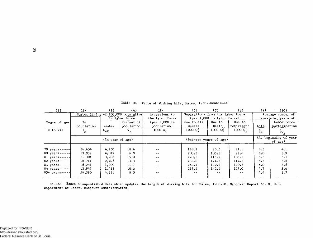
on00
T a b l e 2 0 . T a b l e o f W o r k in g L i f e , M a l e s , 1 9 6 0 - - C o n t i n u e d
( 1 ) , ( 2 )_________________ ( 3 )_____________( 4 )________________( 5 )_____________________ ( 6 )____________( 7 )______________ ( 8 )_____________ ( 9 ) , ( 1 0 )
Y e a r s o f age
Num ber l i v i n g o f 1 0 0 , 0 0 0 b o r n a l i v e A c c e s s i o n s t o t h e l a b o r f o r c e
( p e r 1 , 0 0 0 i n p o p u l a t i o n )
S e p a r a t i o n s f r o m t h e l a b o r f o r c e ( p e r 1 , 0 0 0 i n l a b o r f o r c e )
A v e r a g e nu m b e r o f
I np o p u l a t i o n
I n l a b o r f o r c e re m ai n i n g y e a r s o f
NumberP e r c e n t o f p o p u l a t i o n
Due t o a l l C a u s e s
Due t o D e a t h
Due t o r e t i r e m e n t L i f e
L a b o r f o r c e p a r t i c i p a t i o n
x t o x +1 Lx L wx wx 1 0 0 0 A x 1 0 0 0 Q® 1 0 0 0 Qg 1 0 0 0 Q J oe x
oewx
( I n y e a r o f a g e ) (B e t w e e n ye<sirs o f a g e )( A t b e g i n n i n g o f y e a r
o f a g e )
79 y e a r s --------------- 2 6 , 6 5 4 4 , 9 5 0 1 8 . 6 1 8 8 . 1 9 6 . 5 9 1 . 6 6 . 3 4 . 18 0 y e a r s ............ - 2 3 , 9 5 9 4 , 0 1 9 1 6 . 8 - - 2 0 3 . 3 1 0 5 . 5 9 7 . 8 6 . 0 3 . 981 y e a r s ............ - 2 1 , 3 0 1 3 , 2 0 2 1 5 . 0 2 2 0 . 5 1 1 5 . 2 1 0 5 . 3 5 . 6 3 . 78 2 y e a r s ............ - 1 8 , 7 1 1 2 , 4 9 6 1 3 . 3 - - 2 3 8 . 8 1 2 4 . 5 1 1 4 . 3 5 . 3 3 . 68 3 y e a r s --------------- 1 6 , 2 4 1 1 , 9 0 0 1 1 . 7 - - 2 5 3 . 7 1 3 2 . 9 1 2 0 . 8 5 . 0 3 . 68 4 y e a r s --------------- 1 3 , 9 4 5 1 , 4 1 8 1 0 . 2 - - 2 6 5 . 2 1 4 2 . 2 1 2 3 . 0 4 . 7 3 . 68 5 + y e a r s ------------ 5 6 , 3 9 0 4 , 5 1 1 8 . 0 4 . 4 3 . 7
S o u r c e : B a s e d on u n p u b l i s h e d d a t a w h i c h u p d a t e s T h e L e n g t h o f W o r k i n g L i f e f o r M a l e s , 1 9 0 0 - 6 0 , M an pow er R e p o r t N o . 8 , U . S .D e p a r t m e n t o f L a b o r , M anpower A d m i n i s t r a t i o n .
Digitized for FRASER http://fraser.stlouisfed.org/ Federal Reserve Bank of St. Louis
APPRAISING THE ADEQUACY OF SUPPLY IN IN D IV ID U A L OCCUPATIONS
The preceding chapters of this volume have been concerned with future manpower requirements. In planning occupational training programs, another factor also should be considered—the adequacy of supply. Only by considering both demand and supply together can questions be resolved as to whether or not programs should be developed to expand training in a particular occupation.
The supply of workers in a particular occupation is not static, as a continuous flow of workers into and out of an occupation takes place. Entrants take into account those coming from the following sources: Persons entering directly after completion of a training program designed to prepare them for that occupation; persons entering directly after completion of a training program designed to prepare persons for some other occupation; persons other than students who are not in the civilian labor force, including housewives, retired persons, and those in the Armed Forces; persons employed in other occupations; and immigrants. In a State or specific locality, the migration of persons from other areas might be especially significant. Occupational losses include an estimate of the number of workers in the occupation who will die or retire during the projection period, those who will leave the civilian labor force for some other reason, those who will transfer to other occupations, and those who will emigrate. In the analysis of occupational supply in a State or specific locality, migration to other areas also must be considered.
The flow of manpower into and out of an occupation is illustrated in chart 3.
Several approaches may be used to evaluate the adequacy of supply in an occupation. One approach is to compare the annual number of new entrants in an occupation in recent periods with the number of new workers that will be needed annually in a future period for growth of employment requirements and for replacements. This approach provides an indication as to how much training activities must be expanded to meet estimated or assumed manpower requirements in the occupation. This type of analysis is illustrated in a recent study of health manpower conducted by the Bureau of Labor Statistics, in which the following analysis was made in appraising the adequacy of the output of United States dental schools. The analysis of manpower requirements resulting from employment growth and replacement needs indicated an annual average need for about 5,300 new dentists between 1966 and 1975. Over the 1960-66 period, about 3,200 persons graduated from
dental schools each year. On the basis of follow-up studies of new dental graduates, assumptions were made that nearly all of the new dentists would stay in the field6 1 and that very few other additions to the supply during this 9-year period would take place, because recent experience indicated only a small number of dentists immigrate to the United States and very few persons who qualify as dentists return to this occupation from other fields or from outside of the labor force.62 The conclusions that might be reached by comparing the current output of dental schools with the number of new dentists needed each year would indicate that the annual number of dental graduates would have to be increased by about two-fifths, from about 3,200 to about 5,300, in the 1966-75 period. In using this approach for area manpower analysis, the effect of migration into the area from other parts of the country would have to be evaluated if migration out of the area were included in the estimate of needs. (See Chapter 2 for a discussion of manpower requirements resulting from migration.)
Another approach for determining whether or not, or how much, training programs should be expanded is to appraise current and recent supply-demand relationships to estimate the incidence of “shortages.” Next, an appraisal of the expected growth in requirements relative to past employment increases is made. If, for example, shortages have been and are occurring, and the growth rate in employment requirements is accelerating, one could assume reasonably that the rate of growth in training also must be accelerated.
Another approach that may be useful for some planning purposes is to estimate the supply that might be available at a future target year under specific assumptions about the future. The resulting estimate of supply may be compared with target year projections of requirements to illustrate target-year supply-demand conditions, if steps are not taken through vocational guidance or other methods to adjust supply to prospective demand.
61 This is not true in many occupations, as discussed later in this Chapter.
62 In other fields such as physicians, immigrants have made up a significant proportion of annual new entrants into the occupation in recent periods. In an occupation such as teaching, re-entrants into the labor force, especially women who had withdrawn because of family responsibilities, make up a large percent of additions to supply each year.
59
Digitized for FRASER http://fraser.stlouisfed.org/ Federal Reserve Bank of St. Louis
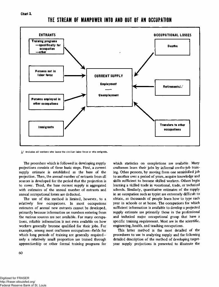
Chart 3.
THE STREAM OF MANPOWER INTO AND OUT OF AN OCCUPATION
ENTRANTS OCCUPATIONAL LOSSES
1/ Includes all workers who leave the civilian labor force or who emigrate.
The procedure which is followed in developing supply projections consists of three basic steps. First, a current supply estimate is established as the base of the projection. Then, the annual number of entrants from all sources is developed for the period that the projection is to cover. Third, the base current supply is aggregated with estimates of the annual number of entrants and annual occupational losses are deducted.
The use of this method is limited, however, to a relatively few occupations. In most occupations estimates of annual new entrants cannot be developed, primarily because information on numbers entering from the various sources are not available. For many occupations, reliable information is not even available on how workers generally become qualified for their jobs. For example, among most craftsmen occupations—fields for which long periods of training are generally required- only a relatively small proportion are trained through apprenticeship or other formal training programs for
which statistics on completions are available. Many craftsmen learn their jobs by informal on-the-job training. Other persons, by moving from one semiskilled job to another over a period of years, acquire knowledge and skills sufficient to become skilled workers. Others begin learning a skilled trade in vocational, trade, or technical schools. Similarly, quantitative estimates of the supply in an occupation such as typist are extremely difficult to obtain, as thousands of people leam how to type each year in schools or at home. The occupations for which sufficient information is available to develop a projected supply estimate are primarily those in the professional and technical major occupational group that have a specific training requirement. Most are in the scientific, engineering, health, and teaching occupations.
This latter method is the most detailed of the procedures to use in analyzing supply and the following detailed description of the method of developing target- year supply projections is presented to illustrate the
6 0
Digitized for FRASER http://fraser.stlouisfed.org/ Federal Reserve Bank of St. Louis
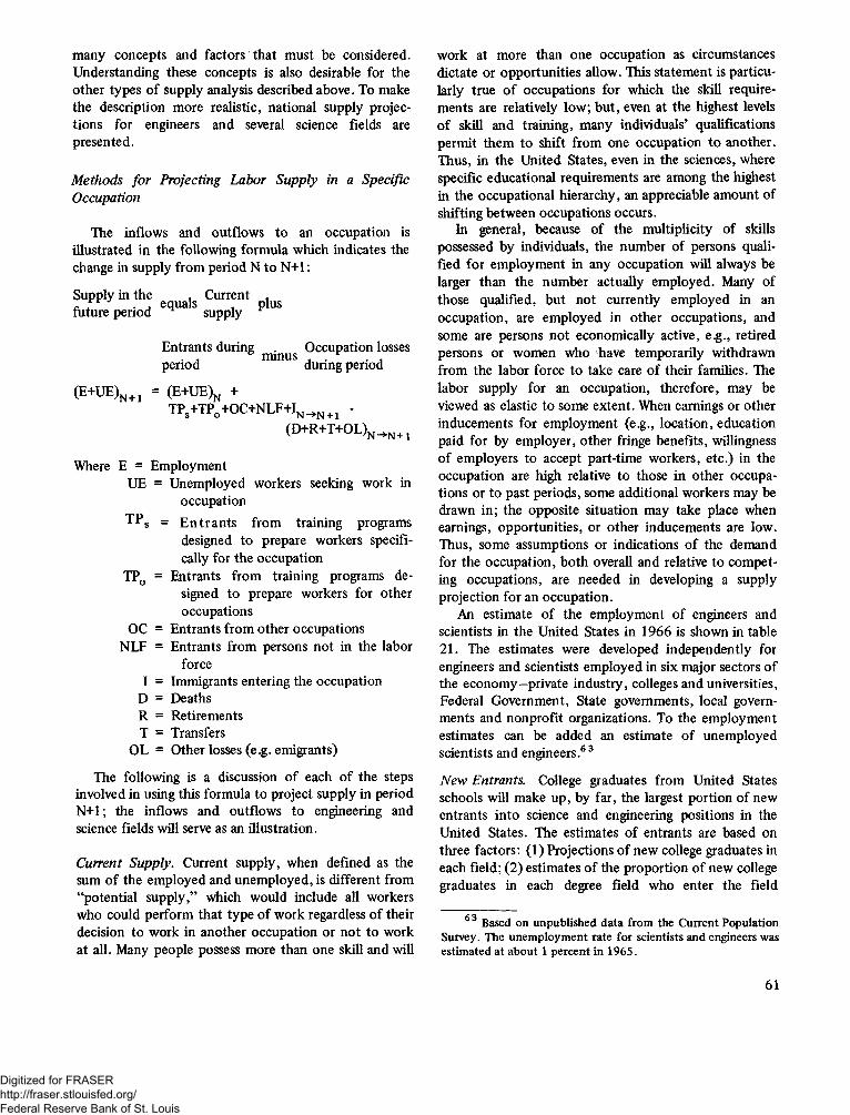
many concepts and factors that must be considered. Understanding these concepts is also desirable for the other types of supply analysis described above. To make the description more realistic, national supply projections for engineers and several science fields are presented.Methods fo r Projecting Labor Supply in a Specific Occupation
The inflows and outflows to an occupation is illustrated in the following formula which indicates the change in supply from period N to N+l:Supply in the . Current . n f . , equals , plus future period supply
Entrants during . Occupation losses. j ° minus 1 . r . ,period during period(E+UE)n+1 = (e+ue)n +
TPs+TPo+0C+NLF+In^ n+1 -(D+R+T+OL)n^ n+1
Where E = EmploymentUE = Unemployed workers seeking work in
occupationTPS = Entrants from training programs
designed to prepare workers specifically for the occupation
TP0 = Entrants from training programs designed to prepare workers for other occupations
OC = Entrants from other occupations NLF = Entrants from persons not in the labor
forceI = Immigrants entering the occupation D = Deaths R = Retirements T = Transfers
OL = Other losses (e.g. emigrants)The following is a discussion of each of the steps involved in using this formula to project supply in period
N+l; the inflows and outflows to engineering and science fields will serve as an illustration.Current Supply. Current supply, when defined as the sum of the employed and unemployed, is different from “potential supply,” which would include all workers who could perform that type of work regardless of their decision to work in another occupation or not to work at all. Many people possess more than one skill and will
work at more than one occupation as circumstances dictate or opportunities allow. This statement is particularly true of occupations for which the skill requirements are relatively low; but, even at the highest levels of skill and training, many individuals’ qualifications permit them to shift from one occupation to another. Thus, in the United States, even in the sciences, where specific educational requirements are among the highest in the occupational hierarchy, an appreciable amount of shifting between occupations occurs.In general, because of the multiplicity of skills possessed by individuals, the number of persons qualified for employment in any occupation will always be larger than the number actually employed. Many of those qualified, but not currently employed in an occupation, are employed in other occupations, and some are persons not economically active, e.g., retired persons or women who have temporarily withdrawn from the labor force to take care of their families. The labor supply for an occupation, therefore, may be viewed as elastic to some extent. When earnings or other inducements for employment (e.g., location, education paid for by employer, other fringe benefits, willingness of employers to accept part-time workers, etc.) in the occupation are high relative to those in other occupations or to past periods, some additional workers may be drawn in; the opposite situation may take place when earnings, opportunities, or other inducements are low. Thus, some assumptions or indications of the demand for the occupation, both overall and relative to competing occupations, are needed in developing a supply projection for an occupation.
An estimate of the employment of engineers and scientists in the United States in 1966 is shown in table 21. The estimates were developed independently for engineers and scientists employed in six major sectors of the economy—private industry, colleges and universities, Federal Government, State governments, local governments and nonprofit organizations. To the employment estimates can be added an estimate of unemployed scientists and engineers.63N ew Entrants. College graduates from United States schools will make up, by far, the largest portion of new entrants into science and engineering positions in the United States. The estimates of entrants are based on three factors: (1) Projections of new college graduates in each field; (2) estimates of the proportion of new college graduates in each degree field who enter the field
6 3 Based on unpublished data from the Current Population Survey. The unemployment rate for scientists and engineers was estimated at about 1 percent in 1965.
61
Digitized for FRASER http://fraser.stlouisfed.org/ Federal Reserve Bank of St. Louis
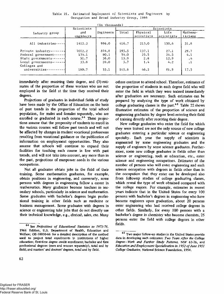
T a b l e 2 1 . E s t i m a t e d E m ploym ent o f S c i e n t i s t s and E n g i n e e r s by O c c u p a t i o n and B r o a d I n d u s t r y G r o u p , 1 9 6 6
( I n t h o u s a n d s )S c i e n t i s t s S c i e n t i s t s
I n d u s t r y g r o u p ande n g i n e e r s
E n g i n e e r s T o t a l P h y s i c a ls c i e n t i s t s
L i f es c i e n t i s t s
M athem at i c i a n s
A l l i n d u s t r i e s --------- 1 4 1 2 . 2 9 9 6 . 0 4 1 6 . 7 2 1 3 . 0 1 5 0 . 6 5 1 . 8
P r i v a t e i n d u s t r y --------------- 1 0 1 2 . 2 8 1 6 . 8 1 9 5 . 5 1 3 7 . 1 2 7 . 1 2 9 . 7F e d e r a l g o v e r n m e n t ----------- 1 3 4 . 1 8 0 . 1 5 4 . 0 2 5 . 5 2 4 . 5 4 . 1S t a t e g o v e r n m e n t s ------------- 5 1 . 7 3 6 . 0 1 5 . 9 2 . 8 1 2 . 9 . 4L o c a l g o v e r n m e n t s -------------C o l l e g e s and
3 3 . 8 2 8 . 0 5 . 7 1 . 4 4 . 2 .1
u n i v e r s i t i e s ------------------- 1 8 0 . 7 3 5 . 1 1 4 5 . 6 4 6 . 2 8 1 . 9 1 7 . 5
immediately after receiving their degree, and (3) estimates of the proportion of these workers who are not employed in the field at the time they received their degrees.
Projections of graduates in individual fields of study have been made by the Office of Education on the basis of past trends in the proportion of the total school population, for males and females separately, who are enrolled or graduated in each course.64 These projections assume that the propensity of students to enroll in the various courses will follow past trends and will not be affected by changes in student vocational preferences resulting from vocational guidance or the publication of information on employment opportunities. They also assume that schools will continue to expand their facilities for teaching each course in line with past trends, and will not take into account, any more than in the past, projections of manpower needs in the various occupations.
Not all graduates obtain jobs in the field of their training. Some mathematics graduates, for example, obtain positions in engineering, and conversely, some persons with degrees in engineering follow a career in mathematics. Many graduates become teachers in secondary schools, particularly in science and mathematics. Some graduates with bachelor’s degrees begin professional training in other fields such as medicine or business management. Some graduates with degrees in science or engineering take jobs that do not directly use their technical knowledge, e.g., clerical, sales, etc. Many
64 See Projections o f Educational Statistics to 1975-76, 1966 Edition, U.S. Department of Health, Education and Welfare; OE-10030-66 for a detailed description of the method used to project total enrollments in institutions of higher education; first-time degree credit enrollment; bachelor and first professional degrees (men and women separately), total and by field.; and masters’ and doctors’ degrees, total and by field.
others continue to attend school. Therefore, estimates of the proportion of students in each degree field who will enter the field in which they were trained immediately after graduation are necessary. Such estimates can be prepared by analyzing the type of work obtained by college graduating classes in the past.65 Table 22 shows illustrative estimates of the proportion of science and engineering graduates by degree level entering their field of training directly after receiving their degree.
New college graduates who enter the field for which they were trained are not the only source of new college graduates entering a particular science or engineering specialty. Each year the supply of scientists is augmented by some engineering graduates and the supply of engineers by some science graduates. Furthermore, some new college graduates in fields other than science or engineering, such as education, etc., enter science and engineering occupations. Estimates of the number of persons who will enter engineering and each science occupation with degrees in fields other than in the occupation that they enter can be developed also from followup studies of college graduating classes, which reveal the type of work obtained compared with the college majors. For example, estimates in recent years indicate that in the United States for every 100 persons with bachelor’s degrees in engineering who have become engineers upon graduation, about 20 persons enter engineering who had received college degrees in other fields. Similarly, for every 100 persons with a bachelor’s degree in chemistry who become chemists, 25 persons enter the field with college degrees in other fields.
65 Two major follow-up studies in the United States provide data in developing such estimates: Two Years A fter the College D egree-W ork and Further S tu dy Patterns, NSF 63-26, and Education and E m ploym en t Specialization in 1952 o f June 1951 College Graduates, National Science Foundation, 1954.
62
Digitized for FRASER http://fraser.stlouisfed.org/ Federal Reserve Bank of St. Louis
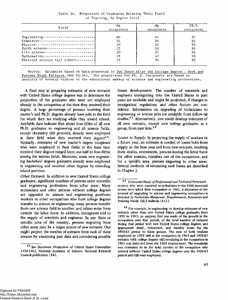
T a b l e 2 2 . P r o p o r t i o n o f G r a d u a t e s E n t e r i n g T h e i r F i e l d o f T r a i n i n g , by D e g r e e L e v e l
F i e l d BAr e c i p i e n t s
MAr e c i p i e n t s
P H .D .r e c i p i e n t s
E n g i n e e r i n g -------------------------------------------------------- 8 0 8 4 97C h e m i s t r y ------------------------------------------------------------ 3 4 6 8 95P h y s i c s ---------------------------------------------------------------- 3 0 61 95E a r t h s c i e n c e ---------------------------------------------------- 25 5 2 95L i f e s c i e n c e ------------------------------------------------------ 2 0 51 95M a t h e m a t i c s -------------------------------------------------------- 19 47 95P h y s i c a l s c i e n c e ( a l l o t h e r ) -------------------- 15 35 95
S o u r c e : E s t i m a t e s b a s e d on d a t a p r e s e n t e d i n Two Y e a r s A f t e r t h e C o l l e g e D e g r e e - Work an dF u r t h e r S t u d y P a t t e r n s (NSF 6 3 - 2 6 ) 0 The p r o p o r t i o n s f o r P h D D. r e c i p i e n t s a r e b a s e d on a n a l y s i s o f s e v e r a l s t u d i e s o f t h e e d u c a t i o n a l m akeup o f s c i e n c e and e n g i n e e r i n g p r o f e s s i o n s .
A final step in preparing estimates of new entrants with United States college degrees was to determine the proportion of the graduates who were not employed already in the occupation at the time they received their degree. A large percentage of persons receiving their master’s and Ph.D. degrees already have jobs in the field for which they are studying while they attend school. Available data indicate that about four-fifths of all new Ph.D. graduates in engineering and all science fields, except chemistry (60 percent), already were employed in their field when they received their degrees66. Similarly, estimates of new master’s degree recipients who were employed in their fields at the time they received their degrees ranged from one-half to four-fifths among the various fields. Moreover, some new engineering bachelors’ degrees graduates already were employed in engineering and received other degrees by attending school parttime.Other Entrants. In addition to new United States college graduates, significant numbers of persons enter scientific and engineering professions from other areas. Many technicians and other persons without college degrees are upgraded to science and engineering positions; workers in other occupations who have college degrees transfer to science or engineering; many persons transfer from one science field to another; and others enter from outside the labor force. In addition, immigrants add to the supply of scientists and engineers. In any State or specific area of the country, persons migrating from other areas may be a major source of new entrants. One might project the number of entrants from each of these sources by examining past data and considering possible
66 See D octorate Production o f U nited States Universities 1920-1962, National Academy of Science, National Research Council publication 1142.
future developments. The number of scientists and engineers immigrating into the United States in past years are available and might be projected, if changes in immigration regulations and other factors are considered. Information on upgrading of technicians to engineering or science jobs are available from follow-up studies.67 Alternatively, one could develop estimates of all new entrants, except new college graduates, as a group, from past data.68Losses to Supply. In projecting the supply of workers to a future year, an estimate is needed of losses both from supply in the base year and from new entrants, resulting from deaths, retirements, persons leaving the labor force for other reasons, transfers out of the occupation; and for a specific area, persons migrating to other areas. Several methods of estimating such losses are described in Chapter 2.
6 7 Postcensal S tudy o f Professional and Technical P ersonnel- persons who were reported as technicians in the 1960 decennial census were asked their occupation in 1962. A discussion of the amount of upgrading to science and engineering occupations is included in Technician M anpower: Requirem ents, Resources and Training Needs. (BLS Bulletin 1512.)
68 For example, in engineering, to develop estimates of new entrants other than new United States college graduates from 1950 to 1963, an analysis first was made of the growth in the occupation over that period; of the total number of entrants during that period with new United States college degrees; and appropriate death, retirement, and transfer losses for the 1950-63 period to these groups. The sum of both workers employed in 1950 still in the occupation in 1963 and 1950-63 entrants with college degrees still remaining in the occupation in 1963 was deducted from.the 1963 employment. The remainder was estimated to be the total number in the occupation who entered without United States college degrees over the 1950-63 period and still were employed.
63
Digitized for FRASER http://fraser.stlouisfed.org/ Federal Reserve Bank of St. Louis
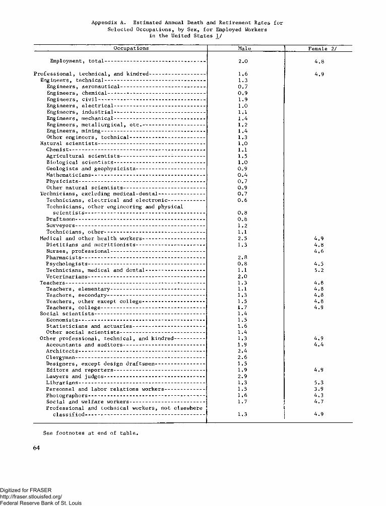
A p p e n d i x A. E s t i m a t e d A n n u a l D e a t h and R e t i r e m e n t R a t e s f o r S e l e c t e d O c c u p a t i o n s , by S e x , f o r E m p loye d W ork ers
i n t h e U n i t e d S t a t e s 1 /O c c u p a t i o n s M ale F e m a le 2 /
E m p lo y m e n t , t o t a l - 2 . 0 4 0 8P r o f e s s i o n a l , t e c h n i c a l , and k i n d r e d ----------------------------------
E n g i n e e r s , t e c h n i c a l ---------------------------------------------------------------E n g i n e e r s , a e r o n a u t i c a l ----------------------------------------------------E n g i n e e r s , c h e m i c a l -------------------------------------------------------------E n g i n e e r s , c i v i l -------------------------------------------------------------------E n g i n e e r s , e l e c t r i c a l ---------------------------------------------------------E n g i n e e r s , i n d u s t r i a l ---------------------------------------------------------E n g i n e e r s , m e c h a n i c a l --------------------------------------------------------E n g i n e e r s , m e t a l l u r g i c a l , e t c . - ------------------------------------E n g i n e e r s , m i n i n g -----------------------------------------------------------------O t h e r e n g i n e e r s , t e c h n i c a l ----------------------------------------------
N a t u r a l s c i e n t i s t s -------------------------------------------------------------------C h e m i s t --------------------------------------------------------------------------------------A g r i c u l t u r a l s c i e n t i s t s ----------------------------------------------------B i o l o g i c a l s c i e n t i s t s --------------------------------------------------------G e o l o g i s t s and g e o p h y s i c i s t s ------------------------------------------M a t h e m a t i c i a n s -----------------------------------------------------------------------P h y s i c i s t s -------------------------------------------------------------------------------O t h e r n a t u r a l s c i e n t i s t s --------------------------------------------------
T e c h n i c i a n s , e x c l u d i n g m e d i c a l - d e n t a l ---------------------------T e c h n i c i a n s , e l e c t r i c a l and e l e c t r o n i c ---------------------T e c h n i c i a n s , o t h e r e n g i n e e r i n g and p h y s i c a l
s c i e n t i s t s ---------------------------------------------------------------------------D r a f t s m e n --------------------- -----------------------------------------------------------S u r v e y o r s ---------------------------------------------------------------------------------T e c h n i c i a n s , o t h e r ------------------- ---------- ---------------------------------
M e d i c a l and o t h e r h e a l t h w o r k e r s --------------------------------------D i e t i t i a n s and n u t r i t i o n i s t s -------------------------------------------N u r s e s , p r o f e s s i o n a l -----------------------------------------------------------P h a r m a c i s t s --------- -------------- -----------------------------------------------------P s y c h o l o g i s t s ---------------------------------------- ---------------------------------T e c h n i c i a n s , m e d i c a l and d e n t a l ------------------------------------V e t e r i n a r i a n s --------------------------------------------------------------------------
T e a c h e r s ----------------------------------------------------------------------------------------T e a c h e r s , e l e m e n t a r y -----------------------------------------------------------T e a c h e r s , s e c o n d a r y --------------------------------------------------------------T e a c h e r s , o t h e r e x c e p t c o l l e g e --------------------------------------T e a c h e r s , c o l l e g e -----------------------------------------------------------------
S o c i a l s c i e n t i s t s ----------------------------------------------------------------------E c o n o m i s t s --------------------------------------------------------------------------------S t a t i s t i c i a n s and a c t u a r i e s ---------------------------------------------O t h e r s o c i a l s c i e n t i s t s -----------------------------------------------------
O t h e r p r o f e s s i o n a l , t e c h n i c a l , and k i n d r e d ------------------A c c o u n t a n t s and a u d i t o r s ---------------------------------------------------A r c h i t e c t s --------------------------------------------------------------------------------C l e r g y m e n ----------------------------------------------------------------------------------D e s i g n e r s , e x c e p t d e s i g n d r a f t s m e n -------------------------------E d i t o r s and r e p o r t e r s ---------------------------------------------------------L a w y e r s and j u d g e s ----------------------------------------------------------------L i b r a r i a n s --------------------------------------------------------------------------------P e r s o n n e l and l a b o r r e l a t i o n s w o r k e r s ------------------------P h o t o g r a p h e r s -------------------------------------------------------------------------S o c i a l and w e l f a r e w o r k e r s ----------------------------------------------P r o f e s s i o n a l and t e c h n i c a l w o r k e r s , n o t e l s e w h e r e
c l a s s i f i e d ---------------------------------------------------------------------------
1 . 61 . 3 0 . 7 0 . 91 . 9 1 . 0 1 . 11 . 41 . 21 . 41 . 3 1 . 0 1 . 11 . 5 1 . 0 0 . 9 0 . 4 0 . 7 0 . 9 0 . 7 0 . 60 . 80 . 81 .21 . 12 . 51 . 32 . 80 . 81 . 12 . 01 . 31 . 11 . 31 . 51 . 71 . 41 . 51 . 61 . 41 . 31 . 92 . 42 . 61 . 51 . 92 . 91 . 31 . 51 . 61 . 7
1 . 3
4 . 9
4 . 94 . 84 . 6
4 . 55 . 24 . 84 . 84 . 84 . 84 . 9
4 . 94 . 4
4 . 9
5 . 3 3 . 94 . 3 4 . 7
4 . 9
S e e f o o t n o t e s a t e n d o f t a b l e .
64
Digitized for FRASER http://fraser.stlouisfed.org/ Federal Reserve Bank of St. Louis
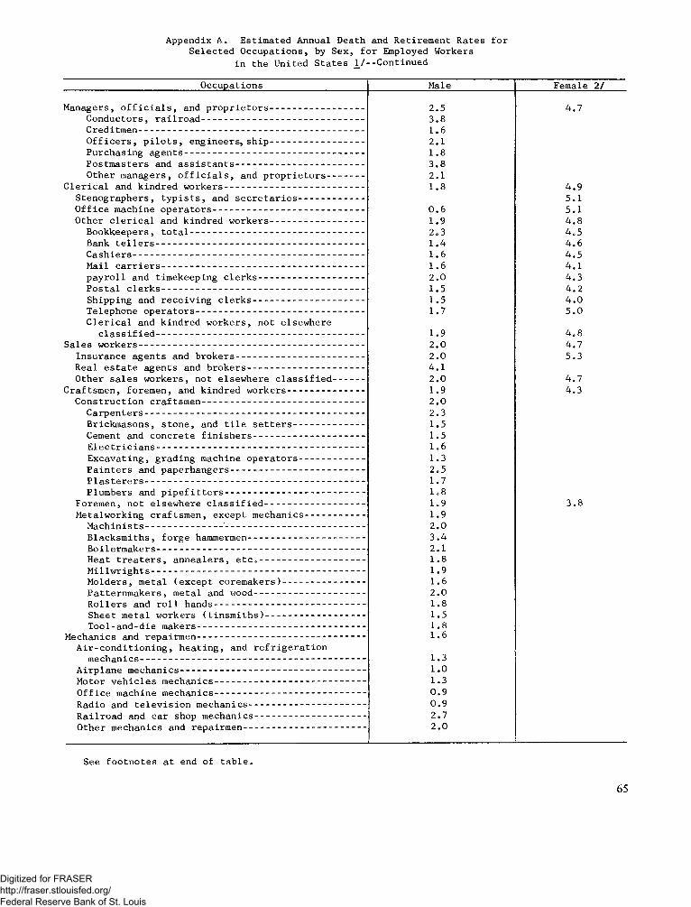
A p p e n d ix A . E s t im a t e d A n n u a l D e a th and R e t ir e m e n t R a t e s f o r S e l e c t e d O c c u p a t io n s , by S e x , f o r E m p loyed W ork ers
i n t h e U n i t e d S t a t e s _ ! / - - C o n t in u e dO c c u p a t io n s M ale F e m a le 2 /
M a n a g e r s , o f f i c i a l s , and p r o p r i e t o r s -----------------------C o n d u c t o r s , r a i l r o a d -----------------------------------------------C r e d itm e n ----------------------------------------------------------------------O f f i c e r s , p i l o t s , e n g i n e e r s , s h i p ----------------------P u r c h a s in g a g e n t s -----------------------------------------------------P o s t m a s t e r s and a s s i s t a n t s -----------------------------------O th e r m a n a g e r s , o f f i c i a l s , an d p r o p r i e t o r s - -
C l e r i c a l an d k in d r e d w o r k e r s --------- -----------------------------S t e n o g r a p h e r s , t y p i s t s , and s e c r e t a r i e s ------------O f f i c e m a c h in e o p e r a t o r s -------------------------------------------O th e r c l e r i c a l an d k in d r e d w o r k e r s ----------------------
B o o k k e e p e r s , t o t a l ---------------------------------------------------Bank t e l l e r s ----------------------------------------------------------------C a s h i e r s ------------------------------------------------------------------------M a il c a r r i e r s --------------------------------------------------------------p a y r o l l an d t im e k e e p in g c l e r k s ---------------------------P o s t a l c l e r k s --------------------------------------------------------------S h ip p in g and r e c e i v i n g c l e r k s -----------------------------T e le p h o n e o p e r a t o r s -------------------------------------------------C l e r i c a l and k in d r e d w o r k e r s , n o t e l s e w h e r e
c l a s s i f i e d ---------------------------------------------------------- —S a l e s w o r k e r s ----------------------------------------------------------------------
I n s u r a n c e a g e n t s and b r o k e r s -----------------------------------R e a l e s t a t e a g e n t s and b r o k e r s -------------------------------O th e r s a l e s w o r k e r s , n o t e l s e w h e r e c l a s s i f i e d
C r a f t s m e n , f o r e m e n , and k in d r e d w o r k e r s ----------------C o n s t r u c t io n c r a f t s m e n -----------------------------------------------
C a r p e n t e r s --------------------------------------------------------------------B r ic k m a s o n s , s t o n e , and t i l e s e t t e r s --------------C em en t and c o n c r e t e f i n i s h e r s -----------------------------E l e c t r i c i a n s ------- -------------- ---------------------- -------------------E x c a v a t i n g , g r a d in g m a c h in e o p e r a t o r s -----------P a i n t e r s and p a p e r h a n g e r s ----------------- ------------------P l a s t e r e r s -------------------------------------------------------------------P lu m b e r s and p i p e f i t t e r s --------------------------------------
F o r e m e n , n o t e l s e w h e r e c l a s s i f i e d ------------------------M e ta lw o r k in g c r a f t s m e n , e x c e p t m e c h a n ic s ---------
M a c h i n i s t s -------------------------------------------------- ----------------B l a c k s m i t h s , f o r g e ham m erm en------------------------------B o i l e r m a k e r s ---------------------------------------------------------------H e a t t r e a t e r s , a n n e a l e r s , e t c . -------------------------M i l l w r i g h t s -----------------------------------------------------------------M o ld e r s , m e t a l ( e x c e p t c o r e m a k e r s ) -----------------P a t t e r n m a k e r s , m e t a l and w oo d ----------------------------R o l l e r s and r o l l h a n d s ------------------------------------------S h e e t m e t a l w o r k e r s ( t i n s m i t h s ) -----------------------T o o l - a n d - d i e m a k e r s ------------------------------------------------
M e c h a n ic s and r e p a ir m e n ------------------------------------------------A i r - c o n d i t i o n i n g , h e a t i n g , an d r e f r i g e r a t i o n
m e c h a n ic s ---------------------------------------------------------------------A i r p l a n e m e c h a n ic s ------------------------------------------------------M oto r v e h i c l e s m e c h a n ic s ------------------------------------------O f f i c e m a c h in e m e c h a n ic s ------------------------------------------R a d io and t e l e v i s i o n m e c h a n ic s ------------------------------R a i l r o a d and c a r sh o p m e c h a n ic s ....................... .............O th e r m e c h a n ic s and r e p a ir m e n --------------------------------
2.5 3 081 . 6 2 .1 1 . 83.82 .11 . 8
0 . 61.92.31.4 1 . 6 1 . 6 2 . 01.51.51.71.9 2 . 0 2 . 04.12 . 01.92 . 02.31.51.51 . 61.32.51.71 . 81.91.9 2 . 03. 42 . 11 . 81.91 . 6 2 . 0 1 . 81.51 . 81 . 61.3 1 . 01.3 0.9 0.9 2.7 2 . 0
4 . 7
4 . 95 . 15 . 14 . 84 . 54 . 6 4 . 54 . 1 4 . 34 . 24 . 05 . 04 . 84 . 75 . 34 . 74 . 3
3 . 8
S e e f o o t n o t e s a t en d o f t a b l e .
65
Digitized for FRASER http://fraser.stlouisfed.org/ Federal Reserve Bank of St. Louis
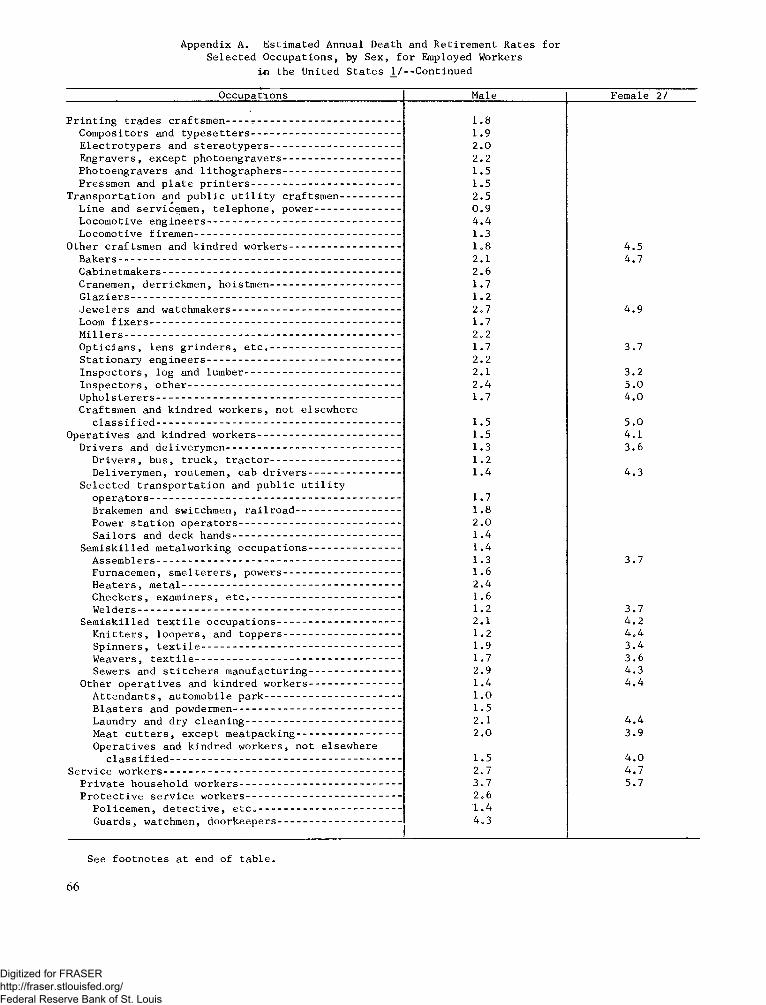
A p p e n d ix A . E s t im a t e d A n n u a l D e a th an d R e t ir e m e n t R a t e s f o r S e l e c t e d O c c u p a t io n s , by S e x , f o r E m p loyed W ork ers
i«n th e U n i t e d S t a t e s 1 / - - C o n t in u e dO c c u p a t io n s M ale
P r i n t i n g t r a d e s c r a f t s m e n --------------------------------- ---------C o m p o s ito r s and t y p e s e t t e r s -----------------------------------E l e c t r o t y p e r s and s t e r e o t y p e r s -----------------------------E n g r a v e r s , e x c e p t p h o t o e n g r a v e r s ------------------------P h o t o e n g r a v e r s and l i t h o g r a p h e r s ------------------------P r e s s m e n and p l a t e p r i n t e r s -----------------------------------
T r a n s p o r t a t io n and p u b l i c u t i l i t y c r a f t s m e n ------L in e an d s e r v i c e m e n , t e l e p h o n e , p o w e r --------------L o c o m o t iv e e n g i n e e r s -------------------------------------------------L o c o m o t iv e f i r e m e n ----------------------------------------------------
O th e r c r a f t s m e n and k in d r e d w o r k e r s ---------------------B a k e r s --------------- ------------ --------------------------------------------------C a b in e t m a k e r s ----------------------------------------------------------------C r a n em en , d e r r ic k m e n , h o i s t m e n ----------------------------G l a z i e r s -------------------------------------------------------------------------J e w e l e r s and w a tc h m a k e r s ----------------------------------------Loom f i x e r s -------------------------------------------------------------------M i l l e r s ----------------------------------------------------------------------------O p t i c i a n s , l e n s g r i n d e r s , e t c . -----------------------------S t a t i o n a r y e n g i n e e r s -------------------------------------------------I n s p e c t o r s , l o g and lu m b e r --------------- ---------- -----------I n s p e c t o r s , o t h e r --------------------------------------------------------U p h o l s t e r e r s ------------------------------------------------------------------C r a f ts m e n and k in d r e d w o r k e r s , n o t e l s e w h e r e
c l a s s i f i e d ------------------------------------------------------------------O p e r a t i v e s and k in d r e d w o r k e r s ---------------------------------
D r iv e r s and d e l i v e r y m e n ------------------------------------------D r i v e r s , b u s , t r u c k , t r a c t o r ----------------------------D e l iv e r y m e n , r o u te m e n , c a b d r i v e r s ---------------
S e l e c t e d t r a n s p o r t a t i o n and p u b l i c u t i l i t yo p e r a t o r s -------------------------------------------------------------------B rakem en an d s w itc h m e n , r a i l r o a d -------------------P ow er s t a t i o n o p e r a t o r s --------------------------------------S a i l o r s and d e c k h a n d s ----------------------------------------
S e m i s k i l l e d m e ta lw o r k in g o c c u p a t i o n s ---------------
1 . 81.92 . 02 . 21.51.52.5 0.9 4. 41.3 1 . 8 2 .12 . 61.71 . 22.71.72 . 21.7 2 . 2 2 .12. 41.71.51.51.31 . 21.41.71 . 8 2 . 01.41.4
F e m a le
4.54.7
4.9
3.73.25. 04. 05 . 04.1 3.64.3
A s s e m b l e r s ------------------------------------------------------------------------F u r n a c e m e n , s m e l t e r e r s , p o w e r s -------------------------------H e a t e r s , m e t a l ----------------------------------------------------------------C h e c k e r s , e x a m in e r s , e t c . -----------------------------------------W e ld e r s ------------------------------------------------------------------------------
S e m i s k i l l e d t e x t i l e o c c u p a t i o n s ---------------------------------K n i t t e r s , l o o p e r s , and t o p p e r s ------------------------------S p i n n e r s , t e x t i l e ---------------------------------------------------------W e a v e r s , t e x t i l e -----------------------------------------------------------S e w e r s and s t i t c h e r s m a n u f a c t u r in g ---------------------
O th e r o p e r a t i v e s and k in d r e d w o r k e r s ---------------------A t t e n d a n t s , a u t o m o b i l e p a r k ------------------------------------B l a s t e r s and p ow d erm en ----------------------------------------------L a u n d ry and d r y c l e a n i n g ------------------------------------------M eat c u t t e r s , e x c e p t m e a t p a c k in g -------------------------O p e r a t i v e s and k in d r e d w o r k e r s , n o t e l s e w h e r e
c l a s s i f i e d ----------- -------------------------------------------------------S e r v i c e w o r k e r s ---------------------------------------------------------------------
P r i v a t e h o u s e h o ld w o r k e r s --------------------------------------------P r o t e c t i v e s e r v i c e w o r k e r s ------------------------------------------
P o l i c e m e n , d e t e c t i v e , e t c . --------------------------------------G u a r d s , w a tc h m e n , d o o r k e e p e r s --------------------------------
1.31 . 62.4 1 . 6 1 . 2 2 .1 1 . 21.9 1.72.91.41 . 01.5 2 .1 2 . 0
3.7
3.74. 24 . 43. 4 3.64.34 . 4
4. 43.9
1.52.73.72 . 61.44.3
4. 04.75.7
2 /
S e e f o o t n o t e s a t en d o f t a b l e .
6 6
Digitized for FRASER http://fraser.stlouisfed.org/ Federal Reserve Bank of St. Louis
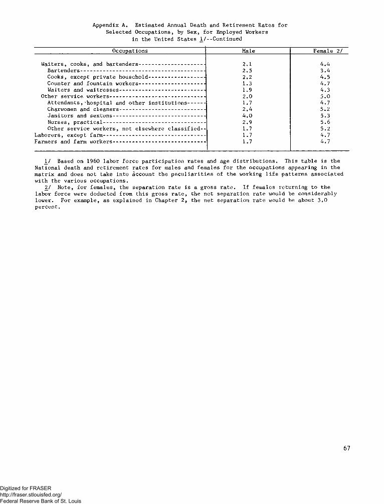
A p p e n d ix A . E s t im a t e d A n n u a l D e a th a n d R e t i r e m e n t R a t e s f o r S e l e c t e d O c c u p a t i o n s , by S e x , f o r E m p lo y e d W o rk ers
i n t h e U n i t e d S t a t e s l / - - C o n t i n u e dO c c u p a t io n s M a le F e m a le 2 /
W a i t e r s , c o o k s , an d b a r t e n d e r s --------- ------------ -------------------- 2 .1 4 . 4B a r t e n d e r s --------------------------------------------------------------------------------- 2 . 5 3 . 4C o o k s , e x c e p t p r i v a t e h o u s e h o l d ------------------------------------ 2 .2 4 . 5C o u n te r an d f o u n t a i n w o r k e r s ------------------------------------------- 1 . 3 4 . 7W a it e r s a n d w a i t r e s s e s ------------------------------------------------------- 1 . 9 4 . 3
O th e r s e r v i c e w o r k e r s -------------------------------------------------------------- 2 . 0 5 . 0A t t e n d a n t s , ‘‘h o s p i t a l an d o t h e r i n s t i t u t i o n s ----------- 1 . 7 4 . 7C harw om en a n d c l e a n e r s -------------------------------------------------------- 2 . 4 5 . 2J a n i t o r s an d s e x t o n s ------------------------------------------------------------ 4 . 0 5 . 3N u r s e s , p r a c t i c a l ------------------------------------------------------------------ 2 . 9 5 . 6O th e r s e r v i c e w o r k e r s , n o t e l s e w h e r e c l a s s i f i e d - - 1 . 7 5 . 2
L a b o r e r s , e x c e p t fa r m ------------------------------------------------------------------ 1 . 7 4 . 7F a r m e r s an d fa r m w o r k e r s ------------------------------------------------------------ 1 . 7 4 . 7
.1/ B a s e d o n 1 9 6 0 l a b o r f o r c e p a r t i c i p a t i o n r a t e s an d a g e d i s t r i b u t i o n s . T h is t a b l e i s t h e N a t i o n a l d e a t h an d r e t i r e m e n t r a t e s f o r m a le s a n d f e m a l e s f o r t h e o c c u p a t i o n s a p p e a r in g i n t h e m a t r i x an d d o e s n o t t a k e i n t o a c c o u n t t h e p e c u l i a r i t i e s o f t h e w o r k in g l i f e p a t t e r n s a s s o c i a t e d w i t h t h e v a r i o u s o c c u p a t i o n s .
27 N o t e , f o r f e m a l e s , t h e s e p a r a t i o n r a t e i s a g r o s s r a t e . I f f e m a l e s r e t u r n i n g t o t h e l a b o r f o r c e w e r e d e d u c t e d fr o m t h i s g r o s s r a t e , t h e n e t s e p a r a t i o n r a t e w o u ld b e c o n s i d e r a b l y l o w e r . F o r e x a m p le , a s e x p l a i n e d i n C h a p te r 2 , t h e n e t s e p a r a t i o n r a t e w o u ld b e a b o u t 3 . 0 p e r c e n t .
67
Digitized for FRASER http://fraser.stlouisfed.org/ Federal Reserve Bank of St. Louis
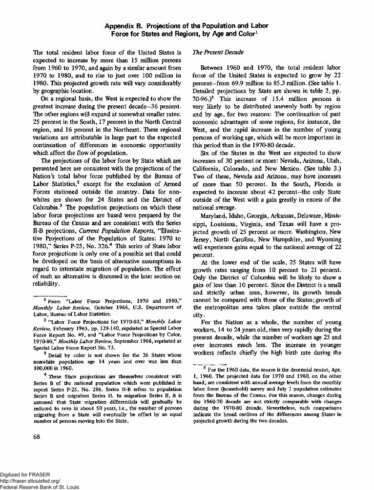
Appendix B. Projections of the Population and Labor Force for States and Regions, by Age and Color1
The total resident labor force of the United States is expected to increase by more than 15 million persons from 1960 to 1970, and again by a similar amount from 1970 to 1980, and to rise to just over 100 million in 1980. This projected growth rate will vary considerably by geographic location.
On a regional basis, the West is expected to show the greatest increase during the present decade—36 percent. The other regions will expand at somewhat smaller rates: 25 percent in the South, 17 percent in the North Central region, and 16 percent in the Northeast. These regional variations are attributable in large part to the expected continuation of differences in economic opportunity which affect the flow of population.
The projections of the labor force by State which are presented here are consistent with the projections of the Nation’s total labor force published by the Bureau of Labor Statistics,2 except for the exclusion of Armed Forces stationed outside the country. Data for nonwhites are shown for 24 States and the District of Columbia.3 The population projections on which these labor force projections are based were prepared by the Bureau of the Census and are consistent with the Series II-B projections, Current Population Reports, “Illustrative Projections of the Population of States: 1970 to 1980,” Series P-25, No. 326.4 This series of State labor force projections is only one of a possible set that could be developed on the basis of alternative assumptions in regard to interstate migration of population. The effect of such an alternative is discussed in the later section on reliability.
1 From “Labor Force Projections, 1970 and 1980,” M onthly Labor Review , October 1966, U.S. Department of Labor, Bureau of Labor Statistics.
2 “Labor Force Projections for 1970-80,” M onthly Labor Review , February 1965, pp. 129-140, reprinted as Special Labor Force Report No. 49, and “Labor Force Projections by Color, 1970-80,” M onthly Labor Review, September 1966, reprinted as Special Labor Force Report No. 73.
3 Detail by color is not shown for the 26 States whose nonwhite population age 14 years and over was less than100,000 in 1960.
4 These State projections are themselves consistent with Series B of the national population which were published in report Series P-25, No. 286. Series II-B refers to population Series B and migration Series II. In migration Series II, it is assumed that State migration differentials will gradually be reduced to zero in about 50 years, i.e., the number of persons migrating from a State will eventually be offset by an equal number of persons moving into the State.
The Present DecadeBetween 1960 and 1970, the total resident labor
force of the United States is expected to grow by 22 percent—from 69.9 million to 85.3 million. (See table 1. Detailed projections by State are shown in table 2, pp. 70-96.)5 This increase of 15.4 million persons is very likely to be distributed unevenly both by region and by age, for two reasons: The continuation of past economic advantages of some regions, for instance, the West, and the rapid increase in the number of young persons of working age, which will be more important in this period than in the 1970-80 decade.
Six of the States in the West are expected to show increases of 30 percent or more: Nevada, Arizona, Utah, California, Colorado, and New Mexico. (See table 3.) Two of these, Nevada and Arizona, may have increases of more than 50 percent. In the South, Florida is expected to increase about 42 percent—the only State outside of the West with a gain greatly in excess of the national average.
Maryland, Idaho, Georgia, Arkansas, Delaware, Mississippi, Louisiana, Virginia, and Texas will have a projected growth of 25 percent or more. Washington, New Jersey, North Carolina, New Hampshire, and Wyoming will experience gains equal to the national average of 22 percent.
At the lower end of the scale, 25 States will have growth rates ranging from 10 percent to 21 percent. Only the District of Columbia will be likely to show a gain of less than 10 percent. Since the District is a small and strictly urban area, however, its growth trends cannot be compared with those of the States; growth of the metropolitan area takes place outside the central city.For the Nation as a whole, the number of young workers, 14 to 24 years old, rises very rapidly during the present decade, while the number of workers age 25 and over increases much less. The increase in younger workers reflects chiefly the high birth rate during the
5 For the 1960 data, the source is the decennial census, Apr. 1, 1960. The projected data for 1970 and 1980, on the other hand, are consistent with annual average levels from the monthly labor force (household) survey and July 1 population estimates from the Bureau of the Census. For this reason, changes during the 1960-70 decade are not strictly comparable with changes during the 1970-80 decade. Nevertheless, such comparisons indicate the broad outlines of the differences among States in projected growth during the two decades.
6 8
Digitized for FRASER http://fraser.stlouisfed.org/ Federal Reserve Bank of St. Louis
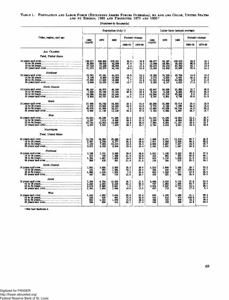
Table 1. Population and Labor Force (Excluding Armed Forces Overseas), by age and Color, United Statesand by Region, 1960 and Projected 1970 and 1980 1[Numbers in thousands]
Population (July 1) Labor force (annual average)Color, region, and age 1960 1970 1980 Percent change 1960 1970 1980 Percent change
(April) 1960-70 1970-80 (April) 1960-70 1970-80All Classes
Total, United States14 years and over_____________________________ 126,277 148,944 173,161 18.0 16.3 69,877 85,257 100,670 22.0 18.114 to 24 years_____________________________ 26,839 39,625 45,369 47.6 14.5 12,009 19,934 23,652 66.0 18.625 to 54 years____ _________________________ 67,523 71,249 83,650 5.5 17.4 45,573 50,472 60,06216,956 10.7 19.055 years and over_____ ____________________ 31,915 38,070 44,142 19.3 15.9 12,295 14,852 20.8 14.2
Northeast14 years and over_____________________________ 32,561 37,041 41,670 13.8 12.2 18,260 21,150 23,762 15.8 12.314 to 24 years_____ ________________________ 6,149 8,860 10,052 44.1 13.5 2,775 4,335 5,051 56.2 16.525 to 54 years____ _________________________ 17,606 17,905 19,933 1.7 11.3 11,951 12,658 14,089 5.9 11.355 years and over___ ______________ _______ 8,806 10,276 11,586 16.7 12.7 3,535 4,157 4,622 17.6 11.2North Central14 years and over.............................. .............. .............. 36,157 40,675 46,559 12.5 14.5 20,047 23,399 27,362 16.7 16.914 to 24 years_____________ ________________ 7,460 10,726 12,164 43.8 13.4 3,455 5,523 6,534 59.9 18.325 to 54 years______ _______________________ 19,096 19,241 22,444 .8 16.6 12,805 13,5764,301 16,042 6.0 18.255 years and over_____ ____________________ 9,602 10,707 11,950 11.5 11.6 3,787 4,786 13.6 11.3
South14 years and over____ ________ ______________ 37,948 45,702 53,393 20.4 16.8 20,398 25,569 30,514 25.4 19.314 to 24 years....... ............._.......... ................. ........ 8,973 12,963 14,592 44.5 12.6 3,770 6,189 7,133 64.2 15.325 to 54 years____ ______________________ 20,076 21,599 25,671 7.6 18.9 13,436 15,338 18,744 14.2 22.255 years and over_______________ __________ 8,900 11,140 13,129 25.2 17.9 3,192 4,043 4,637 26.7 14.7West14 years and over..................... ........................ .............. 19,610 25,526 31,640 30.2 24.0 11,172 2,009 15,139 19,032 35.5 25.714 to 24 years_________________ ____________ 4,257 7,074 8,560 66.2 21.0 3,888 4,934 93.5 26.925 to 54 years___ _________ ________ _______ 10,745 12,505 15,603 16.4 24.8 7,382 8,901 11,187 20.6 25.755 years and over____ ___ __________________ 4,607 5,947 7,476 29.1 25.7 1,781 2,351 2,911 32.0 23.8
N onwhite Total, United States
14 years and over.............. ........................... ................ 13,154 16,384 20,638 24.6 26.0 7,399 9,671 12,219 30.7 26.314 to 24 years____ _________________________ 3,297 5,228 6,777 58.6 29.6 1,3115,008 2,493 3,3357,337 90.2 33.825 to 54 years_____ ___________________ ____ 7,182 7,934 10,013 10.5 26.2 5,837 16.6 25.755 years and over___ ______________________ 2,675 3,223 3,849 20.5 19.4 1,080 1,341 1,547 24.2 15.4Northeast14 years and over....... ......... ........... ........ .................... 2,163 2,791 3,596 29.0 28.8 1,312 1,748 2,222 33.2 27.114 to 24 years______________________ _____ 475 769 1,098 61.9 42.8 216 395 585 82.9 48.125 to 54 years_________________________ ____ 1,291 1,497 1,808 16.0 20.8 913 1,110 1,322 21.6 19.155 years and over................ ........ .......... ................. 398 525 691 31.9 31.6 183 244 315 33.3 29.1
North Central14 years and over_________ _________ __________ 2,340 2,930 3,803 25.2 29.8 1,310 1,699 2,243 29.7 32.014 to 24 years_____ ________________________ 521 907 1,264 74.1 39.4 203 420 637 106.9 51.725 to 54 years....... ......... ............................ ............ 1,363 1,459 1,829 7.0 25.4 922 1,049 1,317 13.8 25.555 years and over______ _______ ____________ 457 565 710 23.6 25.7 184 231 29Q 25.5 25.5South14 years and over....................... ............. .................... 7,209 8,704 10,585 20.7 21.6 3,928 5,025 6,155 27.9 22.514 to 24 years....... .................................................. 1,948 2,932 3,523 50.5 20.2 747 1,365 1,643 82.7 20.425 to 54 years_________________ ___________ 3,679 3,968 5,067 7.9 27.7 2,574 2,947 3,774 14.5 28.155 years and over____ _______________ ______ 1,582 1,804 1,996 14.0 10.6 607 713 738 17.5 3.5West 33.414 years and over....... .................................................. 1,442 1,960 2,654 35.9 35.4 850 1,199 1,599 41.114 to 24 years....... ................................................. 353 620 892 75.6 43.9 145 313 470 115.9 50.225 to 54 years......... .......... ............. ............... .......... 850 1,010 1,309 18.8 29.6 599 732 925 22.2 26.455 years and over_____ _____________ ______ 239 330 452 38.1 37.0 106 153 205 44.3 34.0
1 See text footnote 4.
69
Digitized for FRASER http://fraser.stlouisfed.org/ Federal Reserve Bank of St. Louis
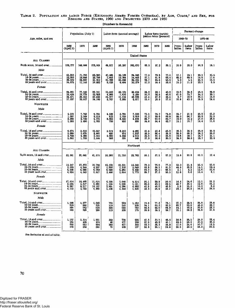
T a b l e 2 . P o p u l a t io n a n d .l a b o r F o r c e (E x c l u d in g A r m e d F o r c e s O v e r s e a s ) , b y A g e , C o l o r ,1 a n d S e x , f o rR e g io n s a n d S t a t e s , 1960 a n d P r o je c t e d 1970 a n d 1980
[Numbers in thousands]
Population (July 1) Labor force (annual average) Labor force partici Percent changeAge, color, and sex pation rates (percent) 1960-70 1970-80
1960(April 1) 1970 1980 1960(April 1) 1970 1980 1960 1970 1980 Population Laborforce Population LaborforceUnited States
All ClassesBoth sexes, 14 and over.................. 126,277 148,944 173,161 69,877 85,257 100,670 55.3 57.2 58.1 18.0 22.0 16.3 18.1
MaleTotal, 14 and over........................... 61,315 71,795 83r380 47,468 55,105 64,246 77.4 76.8 77.1 17.1 16.1 16.1 16.614-24 years................................. 13,385 19,846 22,786 7,643 12,264 14,443 57.1 61.8 63.4 48.3 60.5 14.8 17.825-64 years............................... 33,052 34,807 41,212 31,296 33,348 39,524 94.7 95.8 95.9 5.3 6.6 18.4 18.555 years and over...................... 14,878 17,143 19,382 8,528 9,494 10,279 57.3 55.4 53.0 15.2 11.3 13.1 8.3
FemaleTotal, 14 and over.......................... 64,961 77,148 89,781 22,410 30,152 36,424 34.5 39.1 40.6 18.8 34.5 16.4 20.814-24 years................................ 13,454 19,779 22,583 4.366 7,670 9,209 32.5 38.8 40.8 47.0 75.7 14.2 20.125-54 years................................. 34,471 36,442 42,438 14,277 17,124 20,538 41.4 47.0 48.4 5.7 19.9 16.5 19.955 years and over...................... 17,037 20,927 24,760 3,767 5,358 6,677 22.1 25.6 27.0 22.8 42.2 18.3 24.6
N onwhiteMale
Total, 14 and over........................... 6,279 7,769 9,791 4,528 5,761 7,333 72.1 74.2 74.9 23.7 27.2 26.0 27.314-24 years................................. 1,607 2,549 3,315 822 1,519 2,010 51.2 59.6 60.6 58.6 84.7 30.0 32.325-54 years................................ 3,389 3,729 4,771 3,005 3,432 4,424 88.7 92.0 92.7 10.0 14.2 27.9 28.955 years and over..................... 1,283 1.490 1,705 700 810 899 54.6 54.4 52.7 16.1 15.7 14.4 11.0Female
Total, 14 and over........................... 6,874 8,616 10,847 2,872 3,910 4,886 41.8 45.4 45.0 25.3 36.2 25.9 25.014-24 years................................. 1,6893.793 2,678 3,461 489 974 1,325 28.9 36.4 38.3 58.6 99.2 29.2 36.025-54 years................................. 4,204 5,242 2,002 2,405 2,913 52.8 57.2 55.6 10.8 20.1 24.7 21.155 years and over...................... 1,392 1,733 2,144 380 531 648 27.3 30.6 30.2 24.5 39.6 23.7 22.0Northeast
All ClassesBoth sexes, 14 and over....... .......... 32, 561 37,041 41, 570 18,260 21,150 23,762 56.1 57.1 57.2 13.8 15.8 12.2 12.4
MaleTotal, 14 and over___ _________ 15,547 17, 575 19,754 12,122 13,501 15,248 78.0 76.8 77.2 13.0 11.4 12.4 12.914-24 years________________ 3,005 4,344 4,957 1,616 2,526 3,040 53.8 58.1 61.3 44.6 56.3 14.1 20.425-54 years______ _________ 8,509 8,688 9,780 8,099 8,362 9,436 95.2 96.2 96.5 2.1 3.2 12.6 12.955 years and over................ . 4,034 4,543 5,017 2,406 2,614 2,772 59.7 57.5 55.3 12.6 8.6 10.4 6.1
FemaleTotal, 14 and over... _________ 17, 014 19,466 21,816 6,138 7,649 8,514 36.1 39.3 39.0 14.4 24.6 12.1 11.314-24 years________________ 3,144 4,517 5,095 1,158 1,809 2,011 36.8 40.1 39.5 43.7 56.2 12.8 11.225-54 years________________ 9,097 9,217 10,152 3,851 4,296 4,653 42.3 46.6 45.8 1.3 11.5 10.2 8.355 years and over____ ______ 4.773 5,733 6,569 1,128 1,544 1,850 23.6 26.9 28.2 20.1 36.8 14.6 19.8
N on white Male
Total, 14 and over_____________ 1,006 1,277 1,645 762 990 1,285 75.8 77.5 78.1 27.0 29.8 28.8 29.914r-24 years________________ 220 360 523 119 218 326 54.1 60.5 62.3 63.7 82.8 45.3 49.725-54 years________________ 598 682 824 530 633 782 88.8 92.8 94.9 14.1 19.3 20.8 23.555 years and over__________ 188 236 298 113 139 178 59.9 59.1 59.7 25.1 23.3 26.6 27.9Female
Total, 14 and over___ ________ 1,157 1, 514 1,951 549 759 936 47.5 50.1 48.0 30.8 38.1 28.9 23.414-24 years........... 255 409 574 96 177 259 37.9 43.3 45.1 60.6 83.8 40.3 46.225-54 years___________ _ 693 815 984 383 477 540 55.2 58.5 54.9 17.6 24.6 20.7 13.355 years and over.............. 209 289 392 70 105 137 33.5 36.1 34.9 38.3 49.2 35.5 30.8
See footnotes at end of table.
70
Digitized for FRASER http://fraser.stlouisfed.org/ Federal Reserve Bank of St. Louis
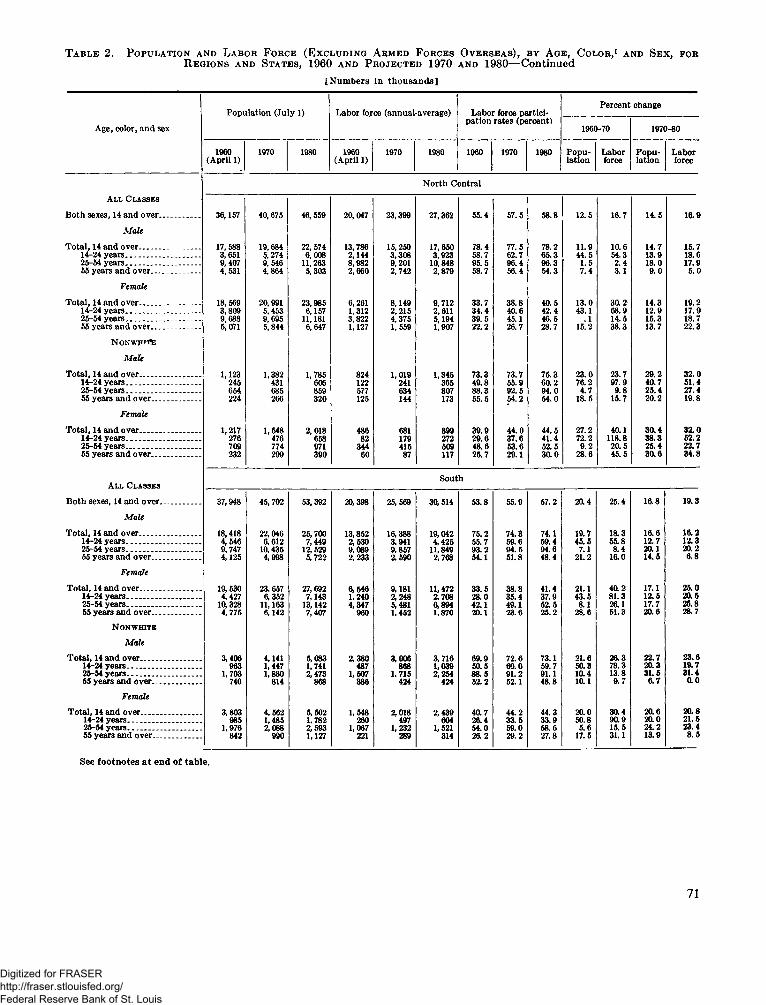
Table 2. Population and Labor Force (Excluding Armed Forces Overseas), by Age, Color,1 and Sex, for Regions and States, 1960 and Projected 1970 and 1980—Continued[Numbers iu thousands]
Population (July 1) Labor force (annual-average) Labor force partici Percent changeAge, color, and sex pation rates (percent) 1960-70 1970-80
1960(April 1) 1970 1980 1960(April 1) 1970 1980 1960 1970 1980 Population Laborforce Population LaborforceNorth Central
All ClassesBoth sexes, 14 and over.................. 36,157 40,675 46, 559 20,047 23,399 27,362 55.4 57.5 58.8 12.5 16.7 14.5 16.9
MaleTotal, 14 and over......... .. ....... 17,588 19, 684 22, 574 13,786 15,250 17,650 78.4 77.5 78.2 11.9 10.6 14.7 15.714-24 years...... .......................... 3,651 5,274 6,008 2,144 3,308 3,923 58.7 62.7 65.3 44.5 54.3 13.9 18.625-54 years...................... .......... 9,407 9, 546 11,263 8,982 9,201 10,848 95.5 96.4 96.3 1.5 2.4 18.0 17.955 years and over........... .......... 4,531 4,864 5,303 2,660 2,742 2,879 58.7 56.4 54.3 7.4 3.1 9.0 5.0
FemaleTotal, 14 and over........................... 18,569 20,991 23,985 6,261 8,149 9,712 33.7 38.8 40.5 13.0 30.2 14.3 19.214-24 years______ _________ 3,809 5, 453 6,157 1,312 2,215 2,611 34.4 40.6 42.4 43.1 68.9 12.9 17.925-54 years................................. 9,688 9, 695 11,181 3, 822 1,127 4,375 5,194 39.5 45.1 46.5 .1 14.5 15.3 18.755 years and over___ ______ 5,071 5, 844 6, 647 1,559 1,907 22.2 26.7 28.7 15.2 38.3 13.7 22.3
N onwph sMale
Total, 14 and over........................... 1,123 1,382 1,785 824 1, 019 1,345 73.3 73.7 75.3 23.0 23.7 29.2 32.014-24 years............... ................ 245 431 606 122 241 365 49.8 55.9 60.2 76.2 97.9 40.7 51.425-54 years________________ 654 685 859 577 634 807 88.3 92.5 94.0 4.7 9.8 25.4 27.455 years and over...................... 224 266 320 125 144 173 55.5 54.2 54.0 18.5 15.7 20.2 19.8Female
Total, 14 and over........................... 1,217 1,548 2,018 486 681 899 39.9 44.0 44.5 27.2 40.1 30.4 32.014-24 years........ ........................ 276 476 658 82 179 272 29.6 37.6 41.4 72.2 118.8 38.3 52.225-54 years.......................... ....... 709 774 971 344 415 509 48.6 53.6 52.5 9.2 20.5 25.4 22.755 years and over...................... 232 299 390 60 87 117 25.7 29.1 30.0 28.6 45.5 30.6 34.8SouthAll Classes
Both sexes, 14 and over.................. 37,948 45,702 53,392 20,398 25,569 30,514 53.8 55.9 57.2 20.4 25.4 16.8 19.3Male
Total, 14 and over........................... 18,418 22, 046 25,700 13,852 16,388 19,042 75.2 74.3 74.1 19.7 18.3 16.6 16.214-24 years................................. 4,546 6,612 7, 449 2,530 3.941 4,425 55.7 59.6 59.4 45.5 55.8 12.7 12.325-54 years................................. 9,747 10,435 12,529 9,089 9,857 11,849 93.2 94.5 94.6 7.1 8.4 20.1 20.255 years and over...................... 4,125 4,998 5,722 2,233 2,590 2,768 54.1 51.8 48.4 21.2 16.0 14.5 6.8Female
Total, 14 and over........................... 19, 530 23.657 27,692 6,546 9,181 11,472 33.5 38.8 41.4 21.1 40.2 17.1 25.014-24 years................................. 4,427 6,352 7,143 1,240 2,248 2,708 28.0 35.4 37.9 43.5 81.3 12.5 20.625-54 years................................. 10,328 11,163 13,142 4,347 5,481 6,894 42.1 49.1 52.5 8.1 26.1 17.7 25.855 years and over..................... 4,775 6,142 7,407 960 1,452 1,870 20.1 23.6 25.2 28,6 51.3 20.6 28.7N on white
MaleTotal, 14 and over........................... 3,406 4,141 5,083 2,380 3,006 3,716 69.9 72.6 73.1 21.6 26.3 22.7 23.614-24 years................................. 963 1,447 1,7412,473 487 868 1,039 50.5 60.0 59.7 50.3 78.3 20.3 19.725-54 years................................. 1, 703 1,880814 1,507 1. 715 2,254 88.5 91.2 91.1 10.4 13.8 31.5 31.455 years and over.................... 740 868 386 424 424 52.2 52.1 48.8 10.1 9.7 6.7 0.0
FemaleTotal, 14 and over........................... 3,803 4, 562 5,502 1,548 2,018 2,439 40.7 44.2 44.3 20.0 30.4 20.6 20.814-24 years................................. 985 1,485 1.782 260 497 604 26.4 33.5 33.9 50.8 90.9 20.0 21.525-54 years................................. 1, 976 2,088 2,593 1,067 1, 232 1, 521 54.0 59.0 58.6 5.6 15.5 24.2 23.455 years and over..................... 842 990 1,127 221 289 314 26.2 29.2 27.8 17.5 31.1 13.9 8.5
See footnotes at end of table.
71
Digitized for FRASER http://fraser.stlouisfed.org/ Federal Reserve Bank of St. Louis

Table 2. Population and Labor Force (Excluding Armed Forces Overseas), by Age, Color,1 and Sex, for Regions and States, 1960 and Projected 1970 and 1980— Continued[Numbers in thousands]
Population (July 1) Labor force (annual average) Labor force partici Percent changeAge, color, and sex pation rates (percent) 1960-70 1970-80
1960(Aprill) 1970 1980 1960(April 1) 1970 1980 1960 1970 1980 Population Laborforce Population LaborforceWest
All ClassesBoth sexes, 14 and over___ _____ 19,610 25,526 31.640 ll, 172 15,139 19,032 57.0 59.3 60.2 30.2 35.5 24.0 25.7
MaleTotal, 14 and over____________ 9,762 12,491 15,352 7,708 9,966 12,306 79.0 79.8 80.2 28.0 29.3 22.9 23.514-24 years_____ _________ 2,184 3,617 4,372 1,3535,125 2,490 3,055 62.0 68.8 69.9 65.6 84.0 20.9 22.725-54 years................... ........... 5,389 6,137 7,641 5,929 7,390 95.1 96.6 96.7 13.9 15.7 24.5 24.655 years and over............... . 2,189 2,738 3,339 1,229 1,548 1,860 56.2 56.5 55.7 25.1 25.9 22.0 20.2
FemaleTotal, 14 and over............... .......... 9,848 13,035 16,287 3,464 5,173 6,726 35.2 39.7 41.3 32.4 49.3 25.0 30.014-24 years_______________ 2,073 3,458 4,188 656 1,398 1,879 31.6 40.4 44.9 66.8 113.1 21.1 34.425-54 years----------------------- 5,356 6,368 7,962 2,256 2,972 3,796 42.1 46.7 47.7 18.9 31.7 25.0 27.755 years and over____ _____ 2,418 3,209 4,137 552 803 1,051 22.8 25.0 25.4 32.7 45.6 28.9 30.8
N on white Male
Total, 14 and over________ ____ 745 968 1,278 562 746 987 75.4 77.0 77.2 30.0 32.8 32.0 32.214-24 years.............. ............. . 180 312 445 95 193 281 52.7 61.9 63.1 73.2 103.1 42.7 45.625-54 years--------- ------------- 434 482 615 390 450 581 89.8 93.4 94.6 11.0 15.4 27.5 29.155 years and over__________ 130 174 218 76 103 124 58.5 59.0 57.1 33.6 34.6 25.0 21.0Female
Total, 14 and over___ _________ 697 991 1,376 289 452 613 41.4 45.6 44.5 42.2 56.8 38.8 35.414-24 years_______________ 173 308 447 50 121 189‘ 29.0 39.2 42.3 77.7 140.0 45.2 56.925-54 years............................... 415 528 694 208 281 343 50.2 53.3 49.4 27.0 35.0 31.5 21.955 years and over__________ 108 155 234 30 50 80 27.6 32.4 34.3 43.7 68.8 50.8 59.4New England
All ClassesBoth sexes, 14 and over________ 7,582 8,628 9,828 4,331 5,044 5,767 57.1 58.5 58.7 13.8 16.5 13.9 14.3
MaleTotal, 14 and over____________ 3,628 4,119 4,708 2,833 3,207 3,726 78.1 77.9 79.1 13.5 13.2 14.3 16.214-24 years_______ ________ 751 1,096 1,258 428 695 857 57.0 63.4 68.1 45.9 62.2 14.7 23.325-54 years--------- ------------- 1,943 1,992 2,307 1,856 1,924 2,234 95.6 96.6 96.8 2.5 3.7 15.8 16.155 years and over__________ 934 1,030 1,144 548 588 635 58.7 57.1 55.5 10.3 7.2 11.1 8.0
FemaleTotal, 14 and over____________ 3,955 4,509 5,119 1,499 1,838 2,041 37.9 40.8 39.9 14.0 22.6 13.5 11.114-24 years_______________ 748 1,085 1,240 287 459 517 38.4 42.3 41.7 45.1 60.0 14.3 12.625-54 years_______________ 2,046 2,084 2,362 918 1,003 1,089 44.8 48.1 46.1 1.8 9.3 13.3 8.555 years and over__________ 1,160 1,340 1,517 294 375 435 25.3 28.0 28.7 15.5 27.7 13.3 16.0
N on white Male
Total, 14 and over____________ 86 117 161 68 96 133 78.1 82.4 82.9 35.5 42.9 37.5 38.314-24 years.............................. 21 36 55 13 25 39 61.5 69.7 70.4 70.8 93.6 51.5 53.025-54 years...................... ........ 51 63 82 46 61 80 90.8 96.5 97.6 24.8 32.6 30.3 31.855 years and over------ -------- 15 18 24 9 10 14 58.4 58.1 60.7 21.2 20.6 34.5 40.5Female
Total, 14 and over____________ 90 129 180 42 64 86 46.6 49.6 47.7 43.6 52.6 39.9 34.814t-24 years_______________ 22 38 57 8 17 26 38.2 44.9 46.1 73.3 103.6 50.5 54.625-54 years______________ 52 70 93 28 39 49 53.6 55.8 52.4 35.3 40.9 33.6 25.455 years and over__________ 16 21 30 6 8 11 35.8 37.1 36.2 29.8 34.6 41.9 38.4
See footnotes at end of table.
72
Digitized for FRASER http://fraser.stlouisfed.org/ Federal Reserve Bank of St. Louis
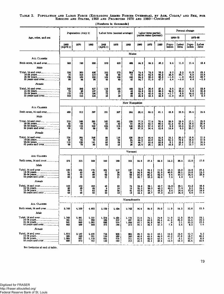
Table 2. Population and Labor F orce (Excluding Armed Forces Overseas), b y Age, Color,1 and Sex, for R egions and States, 1960 and Projected 1970 and 1980—Continued[Numbers in thousands]
Pooulation (July 11 Labor force (annual average) Labor force partici Percent changeAge, color, and sex pation rates (percent) 1960-70 1970-80
1960(April 1) 1970 1980 1960(April 1) 1970 1980 1960 1970 1980 Population Laborforce Population LaborforceMaine
All ClassesBoth sexes, 14 and over......... ........ 683 748 833 370 413 468 54.2 55.2 56.2 9.4 11.5 11.4 13.4
MaleTotal, 14 and over......................... . 334 365 406 252 273 308* 75.4 74.8 76.0 9.2 8.2 11.3 13.114-24 years_______________ 76 105 116 43 66 77 56.6 62.8 66.3 38.6 53.7 9.8 15.825-54 years................................ 168 165 192 159 158 185 95.0 96.0 96.3 - 1.6 - . 6 16.3 16.755 years and over..................... 90 94 98 49 48 47 54.7 51.0 47.7 4.4 - 2.8 4.4 -2 .3
FemaleTotal, 14 and over................ .......... 349 383 427 119 140 160 33.9 36.6 37.4 9.6 18.4 11.5 13.914-24 years................................ 73 98 107 22 35 42 30.3 35.2 38.8 34.6 56.3 9.8 20.825-54 years........... ........... ........ 173 170 194 72 77 86 41.4 45.0 44.3 -1 .7 6.8 14.4 12.555 years and over..................... 103 115 124 25 29 32 23.9 25.5 25.6 11.0 18.0 8.7 9.2
New HampshireAll Classes
Both sexes, 14 and over.................. 433 512 597 251 307 364 58.0 60.0 61.1 18.3 22.3 16.4 18.5Male
Total, 14 and over........................... 210 248 291 162 191 228 77.3 77.0 78.4 18.5 18.0 17.1 19.314-24 years................................. 45 68 79 25 42 52 56.3 62.2 66.0 51.5 67.4 16.4 23.425-54 years............. ................... 109 118 143 105 115 140 96.3 97.3 97.6 8.9 10.0 21.2 21.555 years and over..................... 56 62 68 32 34 36 57.3 54.4 52.6 10.9 5.3 10.1 6.5Female
Total, 14 and over........................... 224 264 306 89 116 136 39.9 44.0 44.5 18.1 30.0 15.8 17.314-24 years.................. ............. 43 65 76 16 29 34 38.0 44.6 44.8 52.2 78.9 16.4 17.025-54 years............................... 113 120 141 55 64 76 48.7 53.4 53.9 6.1 16.4 17.5 18.555 years and over....... .............. 68 79 89 18 23 26 26.6 29.1 29.5 16.5 27.1 12.7 14.3Vermont
All ClassesBoth sexes, 14 and over.................. 274 315 359 149 180 211 54.6 57.1 58.6 15.2 20.5 13.9 17.0
MaleTotal, 14 and over........................... 132 154 178 101 117 137 7& 2 76.1 77.0 ia 2 ia o 15.6 17.114-24 years................................. 31 43 48 17 26 29 54.6 60.5 61.6 40.8 56.1 10.6 12.525-54 years................................. 66 72 90 63 70 86 95.5 96.2 96.0 9.4 10.2 24.0 23.855 years and over...................... 35 38 40 21 21 21 58.7 55.3 52.8 7.6 1.3 5.5 7
FemaleTotal, 14 and over........................... 142 162 182 49 63 74 34.4 39.1 40.7 14.3 30.1 12.3 16.814-24 years................................. 30 43 46 9 16 19 31.5 38.0 40.2 42.1 71.9 8.1 14.425-54 years................................. 69 71 83 29 34 41 42.0 48.1 49.3 3.4 18.4 17.0 19.955 years and over...................... 43 48 52 10 13 14 24.1 26.7 27.3 12.3 24.2 9.0 11.5
MassachusettsAll Classes
Both sexes, 14 and over.................. 3,740 4,150 4,683 2,129 2,434 2,763 56.9 58.6 59.0 11.0 14.3 12.8 13.5Male
Total, 14 and over........................... 1,768 1,961 2,227 1,376 1,531 1,778 77.8 78.1 79.8 11.0 11.3 13.5 16.114-24 years................................. 361 512 586 205 327 407 56.8 63.8 69.4 41.9 59.3 14.4 24.625-54 years................................. 941 949 1,095 896 914 1,059 95.1 96.3 96.7 .9 2.1 15.3 15.855 years and over...................... 465 499 545 275 290 312 59.1 58.1 57.2 7.4 5.4 9.2 7.6Female
Total, 14 and over........................... 1.972 2,189 2,456 754 903 985 38.2 41.2 40.1 11.0 19.8 12.2 9.214-24 years................................. 368 520 591 150 236 260 40.6 45.4 44.0 41.2 57.6 13.7 10.125-54 years................................. 1,004600 997 1,123 451 478 511 44.9 48.0 45.5 - . 7 6.1 12.7 6.955 years and over...................... 672 742 153 189 215 25.5 28.1 28.9 12.0 23.2 10.4 13.8See footnotes at end of table.
73
Digitized for FRASER http://fraser.stlouisfed.org/ Federal Reserve Bank of St. Louis
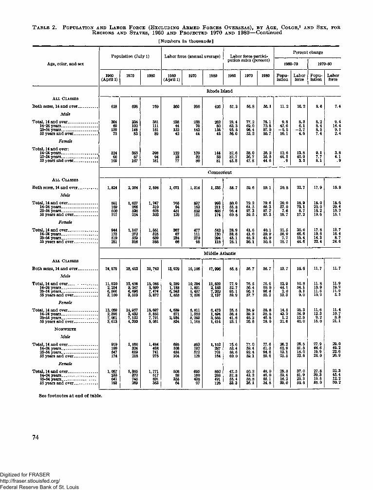
T able 2. Population and Labor Force (Excluding Armed Forces Overseas), by Age, Color,1 and Sex, for Regions and States, 1960 and Projected 1970 and 1980— Continued[Numbers in thousands]
Population [July 1) Labor force (annual averaee) Labor force partici Percent changeAge, color, and sex pation rates (percent) 1960-70 1970-80
1960(April 1) 1970 1980 1960(April 1) 1970 1980 1960 1970 1980 Population Laborforce Population LaborforceRhode Island
All ClassesBoth sexes, 14 and over.............. 628 698 759 360 396 426 57.3 56.8 56.1 11.2 10.2 8.6 7.4
MaleTotal, 14 and over...................... 304 334 361 238 258 282 78.4 77.2 78.1 9.8 8.3 8.2 9.414-24 years.......................... 69 102 111 44 70 80 63.3 69.0 72.8 47.0 6.1 8.4 14.425-54 years........................... 159 148 161 152 143 156 95.5 96.4 97.0 -6.5 -5.7 8.5 9.155 years and over................. 75 83 89 42 44 45 56.0 53.2 50.7 10.1 4.6 7.4 2.4
FemaleTotal, 14 and over:14-24 years.......................... 324 365 398 122 139 144 37.6 38.0 36.2 12.6 13.8 9.1 3.825-54 years........................... 60 87 94 23 32 33 37.7 36.7 35.5 44.5 40.9 7.7 4.155 years and over................. 169 167 181 77 80 81 45.8 47.8 44.6 .9 3.5 8.1 .9
ConnecticutAll Classes
Both sexes, 14 and over_______ 1,824 2,204 2,598 1,071 1,314 1,535 58.7 59.6 59.1 20.8 22.7 17.9 16.8Male
Total, 14 and over______ ____ 881 1,057 1,247 705 837 993 80.0 79.2 79.6 20.0 18.9 18.0 18.614-24 years______ ___ __ 169 266 319 94 163 211 55.8 61.5 66.3 57.0 73.1 20.0 29.425-54 years------------------- 500 538 625 481 523 608 96.4 97.3 97.2 7.6 8.7 16.2 16.255 years and over________ 212 254 303 129 151 174 60.8 59.5 57.3 19.7 17.2 19.6 15.1Female
Total, 14 and over---- ----------- 944 1,147 1,351 367 477 542 38.9 41.6 40.1 21.5 30.0 17.8 13.714-24 years_____________ 173 272 325 67 111 130 38.6 41.0 39.9 56.9 66.6 19.6 16.425-54 years------------------- 519 559 639 234 270 294 45.1 48.3 45.9 7.7 15.4 14.3 8.755 years and over________ 251 316 386 66 95 118 26.1 30.1 30.6 25.7 44.6 22.4 24.6Middle Atlantic
All ClassesBoth sexes, 14 and over_______ 24,979 28,413 31,742 13,929 16,105 17,996 55.8 56.7 56.7 13.7 15.6 11.7 11.7
MaleTotal, 14 and over—.________ 11,920 13,456 15,045 9,289 10,294 11,522 77.9 76.5 76.6 12.9 10.8 11.8 11.914-24 years.......................... 2,254 3,247 3,699 1,188 1,831 2,183 52.7 56.4 59.0 44.1 54.1 13.9 19.225-54 years------------------- 6,566 6,696 7,474 6,243 6,437 7,202 95.1 96.1 96.4 2.0 3.1 11.6 11.955 years and over.......... ..... 3,100 3,513 3,872 1,858 2,026 2,137 59.9 57.7 55.2 13.3 9.0 10.2 5.5
FemaleTotal, 14 and over—................ 13,059 14,957 16,697 4,639 5,811 6,473 35.5 38.9 38.8 14.5 25.3 11.6 11.414-24 years_____________ 2,396 3,432 3,855 871 1,350 1,494 36.4 39.3 38.8 43.2 54.9 12.3 10.725-54 years_____________ 7,051 7,132 4,393 7,791 2,934834 3,293 3,565 41.6 46.2 45.8 1.2 12.3 9.2 8.355 years and over.... ............ 3,613 5,051 1,168 1,414 23.1 26.6 28.0 21.6 40.0 15.0 21.1
N onwhiteMale
Total, 14 and over______ ____ 919 1,160 1,484 695 893 1,152 75.6 77.0 77.6 26.2 28.5 27.9 29.014-24 years.......................... 199 324 468 106 192 287 53.4 59.4 61.3 62.9 81.5 44.6 49.225-54 years............ -............ 547 619 741 484 572 701 88.6 92.4 94.6 13.1 18.0 19.9 22.655 years and over................. 174 218 275 104 129 164 60.0 59.1 59.6 25.5 23.6 26.0 26.9
FemaleTotal, 14 and over..................... 1,067 1,385 1,771 508 695 850 47.5 50.2 48.0 29.8 37.0 27.8 22.314-24 years..... ........ .......... 233 372 517 88 160 233 37.8 43.2 45.0 59.4 81.9 39.3 45.425-54 years____________ 641 745 891 355 438 491 55.4 58.8 55.1 16.2 23.3 19.5 12.2
55 years and over___ ____ 193 269 363 64 97 126 33.3 36.1 34.8 39.0 50.5 85.0 30.2See footnotes at end of table.
74
Digitized for FRASER http://fraser.stlouisfed.org/ Federal Reserve Bank of St. Louis
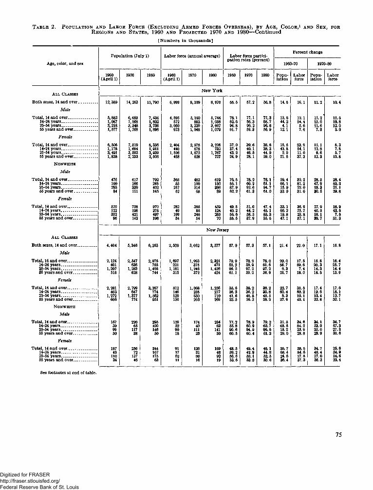
Table 2. Population and Labor Force (Excluding Armed Forces Overseas), by Age, Color,1 and Sex, for Regions and States, 1960 and Projected 1970 and 1980—Continued[Numbers in thousands]
Population (July 1) Labor force (annual average) Labor force partici Percent changeAge, color, and sex pation rates (percent) 1960-70 1970-80
1060(April 1) 1970 1980 1960(April 1) 1970 1980 1960 1970 1980 Population Laborforce Population LaborforceNew YorkAll Classes
Both sexes, 14 and over................ 12,389 14,203 15,790 6,999 8,109 8,970 56.5 57.2 56.8 14.6 16.1 11.2 10.4Male
Total, 14 and over.......... .............. 5,882 6,683 7,434 4,595 5,150 5,744 78.1 77.1 77.3 13.6 12.1 11.2' 11.514-24 years............................... 1,087 1,568 1,802 572 883 1,058 52.6 56.3 58.7 44.2 54.4 15.0 19.825-54 years............................... 3,218 3,348 3,736 3,050 3,220 3,607 94.8 96.2 96.6 4.1 5.6 11.6 12.055 years and over.................... 1,577 1,768 1,896 973 1,048 1,079 61.7 59.3 56.9 12.1 7.6 7.3 3.0Female
Total, 14 and over......................... 6,506 7,519 8,356 2,404 2,978 3,226 37.0 39.6 38.6 15.6 23.9 11.1 8.314-24 years.............................. 1,178 3,491 1,694 1,911 440 678 732 37.4 40.1 38.3 43.8 54.1 12.8 7.825-54 years_______________ 3,593 3,939 1,506 1,672 1,767 43.2 46.5 44.9 2.9 11.0 9.6 5.755 years and over.................... 1,838 2,233 2,506 458 628 727 24.9 28.1 29.0 21.5 37.3 12.3 15.8N onwhite
MaleTotal, 14 and over......................... 476 617 792 365 482 619 76.5 78.2 78.1 29.4 32.2 28.5 28.414-24 years................... ........... 100 166 245 55 100 150 55.1 60.2 61.1 66.1 81.2 47.9 50.325-54 years......... ..................... 293 339 402 257 314 380 87.9 92.6 94.7 15.9 22.0 18.3 21.155 years and over.................... 84 111 145 52 68 89 62.2 61.3 61.0 33.0 31.0 30.5 29.8
FemaleTotal, 14 and over.........................14-24 years......... ..................._ 570 758 970 282 386 459 49.5 51.0 47.4 33.1 36.9 27.9 18.9122 196 275 49 86 124 40.2 44.2 45.1 60.2 75.7 40.5 43.525-54 years...... ........................ 352 421 497 199 246 265 56.6 58.5 53.3 19.8 23.8 18.1 7.555 years and over.................... 96 142 198 34 54 70 35.5 37.9 35.6 47.1 57.1 39.7 31.3
New JerseyAll Classes
Both sexes, 14 and over................. 4,404 5,346 6,263 2,509 3,062 3,577 57.0 57.3 57.1 21.4 22.0 17.1 16.8Male
Total, 14 and over......................... 2,124 2,547 2,976 1,697 1,993 2,321 79.9 78.2 78.0 20.0 17.5 16.8 16.414-24 years............................... 401 636 765 221 375 471 55.2 58.9 61.6 58.7 69.6 20.3 25.725-54 years....... ...................... 1,207 1,283 1,466 1,161 1,246 1,426 96.2 97.2 97.2 6.3 7.4 14.3 14.455 years and over___ ______ 516 628 744 315 372 424 61.1 59.2 56.9 21.7 18.0 18.5 13.9Female
Total, 14 and over........ ............... 2,281 2,799 3,287 812 1,068 1,256 35.6 38.2 38.2 22.7 31.5 17.4 17.614-24 years............ ............... 403 647 774 146 235 277 36.3 36.2 35.8 60.4 60.2 19.6 18.125-54 years................. ............ 1,272 1,377 1,562 529 630 710 41.6 45.8 45.5 8.3 19.1 13.4 12.765 years and over__________ 606. 774 951 136 203 269 22.5 26.3 28.2 27.9 49.1 22.8 32.1N on white
MaleTotal, 14 and over....................... 167 220 295 129 174 234 77.2 78.9 79.2 31.8 34.6 34.1 34.714-24 years...... ........................ 39 65 100 22 40 62 55.8 60.9 62.7 68.5 84.2 53.0 57.325-54 years............................... 99 117 146 90 111 141 90.6 94.9 96.6 18.2 23.9 25.0 27.355 years and over.................... 30 38 50 18 23 30 60.5 60.4 61.2 29.0 28.8 29.9 31.6
FemaleTotal, 14 and over......................... 187 256 344 91 126 159 48.5 49.4 46.1 36.7 38.5 34.7 25.614-24 years.............................. 43 72 107 17 31 48 39.2 42.9 44.8 68.4 84.6 48.4 54.925-54 years............................... 110 137 175 62 80 92 56.6 58.1 52.5 24.6 27.8 27.0 14.655 years and over........ ........... 34 46 63 11 16 19 33.6 33.8 30.6 36.4 37.3 36.3 23.4
See footnotes at end of table.
75
Digitized for FRASER http://fraser.stlouisfed.org/ Federal Reserve Bank of St. Louis
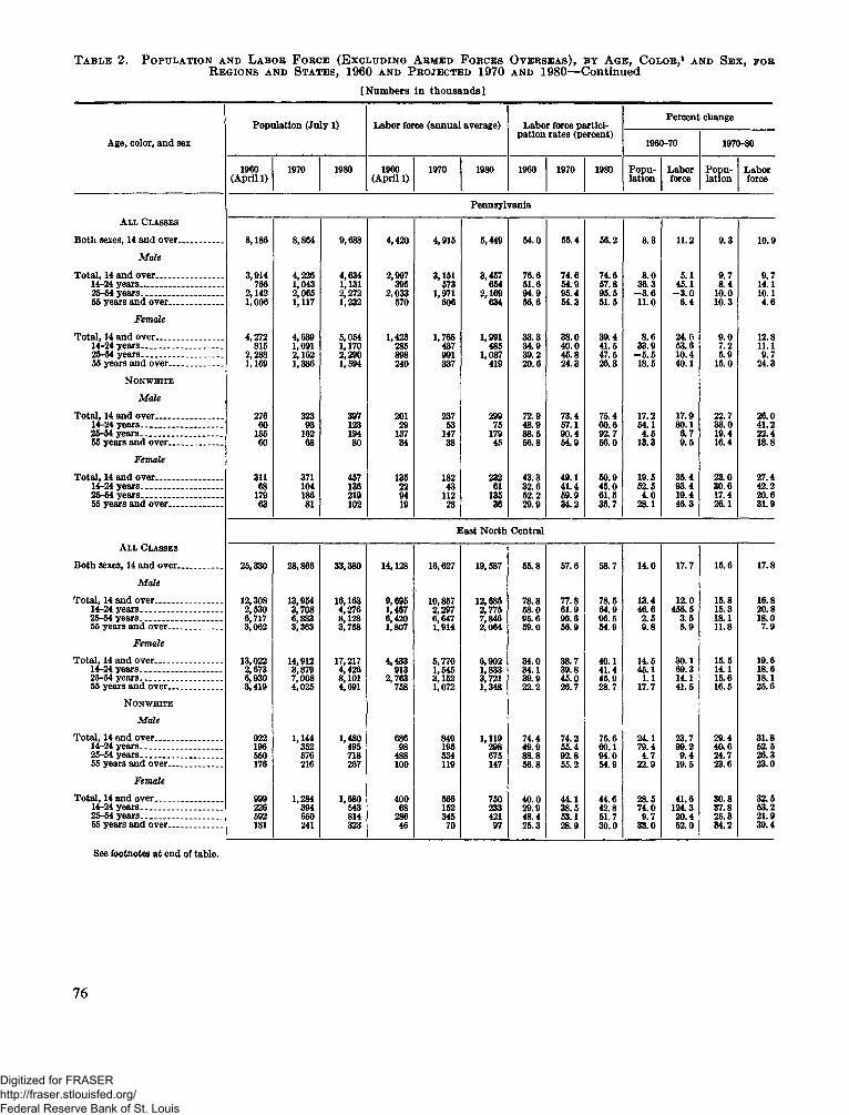
Table 2. Population and Labor Force (Excluding Armed Forces Overseas), by Age, Color,1 and Sex, for Regions and States, 1960 and Projected 1970 and 1980—Continued[Numbers in thousands]
Population (July 1) Labor force (annual average) Labor force partici Percent changeAge, color, and sex pation rates (percent) .1960-70 1970-80
1960(April 1) 1970 1980 1960(April 1) 1970 1980 1960 1970 1980 Population Laborforce Population LaborforcePennsylvania
All ClassesBoth sexes, 14 and over.............. 8,186 8,864 9,688 4,420 4,915 5,449 54.0 55.4 56.2 8.3 11.2 9.3 10.9
MaleTotal, 14 and over..................... 3,914 4,226 4,634 2,997 3,151 3,457 76.6 74.6 74.6 8.0 5.1 9.7 9.714-24 years....... ..... ............ 766 1,043 1,131 395 573 654 51.6 54.9 57.8 36.3 45.1 8.4 14.125-54 years_________ ___ 2,142 2,065 2,272 2,033 1,971 2,169 94.9 95.4 95.5 -3.6 -3.0 10.0 10.155 years and over................. 1,006 1,117 1,232 570 606 634 56.6 54.3 51.5 11.0 6.4 10.3 4.6
FemaleTotal, 14 and over__________ 4,272 4,639 5,054 1,423 1,765 1,991 33.3 38.0 39.4 8.6 24.0 9.0 12.814-24 years............. ............ 815 1,091 1,170 285 437 485 34.9 40.0 41.5 33.9 53.6 7.2 11.125-54 years____________ 2,288 2,162 2,290 898 991 1,087 39.2 45.8 47.5 -5.5 10.4 5.9 9.755 years and over________ 1,169 1,386 1,594 240 337 419 20.6 24.3 26.3 18.5 40.1 15.0 24.3
N onwhiteMale
Total, 14 and over____ ______ 276 323 397 201 237 299 72.9 73.4 75.4 17.2 17.9 22.7 26.014-24 years...... .......... ........ 60 93 123 29 53 75 48.9 57.1 60.6 54.1 80.1 33.0 41.225-54 years..... ......... ........... 155 162 194 137 147 179 88.5 90.4 92.7 4.5 6.7 19.4 22.455 years and over________ 60 68 80 34 38 45 56.8 54.9 56.0 13.3 9.5 16.4 18.8Female
Total, 14 and over__________ 311 371 457 135 182 232 43.3 49.1 50.9 19.5 35.4 23.0 27.414-24 years................ ......... 68 104 136 22 43 61 32.6 41.4 45.0 52.5 93.4 30.6 42.225-54 years......................... 179 186 219 94 112 135 52.2 59.9 61.5 4.0 19.4 17.4 20.655 years and over................. 63 81 102 19 28 36 29.9 34.2 35.7 28.1 46.3 26.1 31.9East North Central
All ClassesBoth sexes, 14 and over_______ 25,330 28,866 33,380 14,128 16,627 19,587 55.8 57.6 58.7 14.0 17.7 15.6 17.8
MaleTotal, 14 and over__________ 12,308 13,954 16,163 9,695 10,857 12,685 78.8 77.8 78.5 13.4 12.0 15.8 16.814-24 years...................... . 2,530 3,708 4,276 1,467 2,297 2,775 58.0 61.9 64.9 46.6 456.5 15.3 20.825-54 years_____ _______ 6,717 6,883 8,128 6,420 6,647 7,846 95.6 96.6 96.5 2.5 3.5 18.1 18.055 years and over________ 3,062 3,363 3,758 1,807 1,914 2,064 59.0 56.9 54.9 9.8 5.9 11.8 7.9
FemaleTotal, 14 and over__________14-24 years_____________ 13,022 14,912 17,217 4,433 5,770 6,902 34.0 38.7 40.1 14.5 30.1 15.5 19.62,673 3,879 4,426 913 1,545 1,833 34.1 39.8 41.4 45.1 69.3 14.1 18.625-54 years_____________ 6,930 7,008 8,101 4,691 2,763 3,152 3,721 39.9 45.0 45.9 1.1 14.1 15.6 18.155 years and over________ 3,419 4,025 758 1,072 1,348 22.2 26.7 28.7 17.7 41.5 16.5 25.6
N onwhiteMale
Total, 14 and over__________ 922 1,144 1,480 686 849 1,119 74.4 74.2 75.6 24.1 23.7 29.4 31.814-24 years_____________ 196 352 495 98 195 298 49.9 55.4 60.1 79.4 99.2 40,6 52.525-54 years....................... 550 576 718 488 534 675 88.8 92.8 94.0 4.7 9.4 24.7 26.355 years and over________ 176 216 267 100 119 147 56.8 55.2 54.9 22.9 19.5 23.6 23.0Female
Total, 14 and over_______ ___ 999 1,284 1,680 400 566 750 40.0 44.1 44.6 28.5 41.6 30.8 32.514-24 years____________ 226 394 543 68 152 233 29.9 38.5 42.8 74.0 124.3 37.8 53.225-54 years...... ............ ...... 592 650 814 286 345 421 48.4 53.1 51.7 9.7 20.4 25.3 21.955 years and over________ 181 241 323 46 70 97 25.3 28.9 30.0 33.0 52.0 34.2 39.4See footnotes at end of table.
76
Digitized for FRASER http://fraser.stlouisfed.org/ Federal Reserve Bank of St. Louis
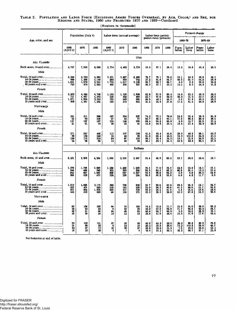
Table 2. Population and Labor Force (Excluding Armed Forces Overseas), by Age, Color,1 and Sex, for Regions and States, 1960 and Projected 1970 and 1980— Continued[Numbers in thousands]
Population (July 1) Labor force (annual average) Labor force partici Percent changeAge, color, and sex pation rates (percent) 1960-70 1970-80
1960(April 1) 1970 1980 1960(April 1) 1970 1980 1960 1970 1980 Population Laborforce Population LaborforceOhio
A l l C l a s s e s
Both sexes, 14 and over.................. 6,767 7,818 9,098 3,724 4,463 5,276 55.0 57.1 58.0 15.5 19.8 16.4 18.2M a le
Total, 14 and over................ ......... 3,266 3,760 4,392 2,571 2,937 3,468 78.7 78.1 79.0 15.1 14.2 16.8 18.114-24 years................................ 669 1,006 1,149 385 620 743 57.5 61.6 64.7 50.3 61.0 14.3 19.925-54 years................................. 1,801 1,879 2,241 1,723 1,817 2,168 95.7 96.7 96.7 4.3 5.5 19.3 19.355 years and over...................... 795 876 1,002 463 500 557 58.2 57.1 55.5 10.1 8.0 14.4 11.3F em ale
Total, 14 and over........................... 3,502 4,058 4,706 1,153 1,526 1,808 32.9 37.6 38.4 15.9 32.3 16.0 18.514-24 years................................. 721 1,067 1,202 236 402 469 32.7 37.8 39.0 48.0 71.0 12.7 16.525-54 years................... .............. 1,871 1,924 2,242 723 849 986 38.6 44.1 44.0 2.8 17.4 16.5 16.255 years and over...................... 909 1,067 1,262 193 273 352 21.3 25.6 27.9 17.3 41.2 18.3 28.8N o n w h i ^e
M a leTotal, 14 and over........................... 251 311 399 187 234 307 74.5 75.2 76.9 24.3 25.4 28.0 31.014-24 years........ ........................ 52 94 128 27 52 77 50.7 56.1 60.1 77.5 96.5 36.4 46.125-54 years................................. 147 157 197 132 148 189 89.4 94.3 95.9 6.9 12.7 25.3 27.455 years and over...................... 51 61 74 28 33 41 55.8 54.8 55.4 19.4 17.4 22.0 23.3
F em aleTotal, 14 and over........................... 271 347 448 112 157 205 41.3 45.4 45.8 28.0 40.5 29.1 30.514-24 years................................. 60 104 140 19 40 59 31.3 38.4 42.0 73.0 112.3 34.3 47.125-54 years................................ 159 175 219 80 97 118 50.1 55.4 54.2 10.1 21.8 24.8 22.155 years and over..................... 52 68 89 14 20 28 26.1 30.1 31.4 30.8 50.5 32.1 37.9
IndianaA l l C l a s s e s
Both sexes, 14 and over................. 3,251 3,696 4,264 1,802 2,155 2,567 55.4 58.3 60.2 13.7 19.6 15.4 19.1M a le
Total, 14 and over........................... 1,579 1,798 2,088 1,239 1,400 1,639 78.5 77.9 78.5 13.8 12.9 16.1 17.114-24 years................................. 346 488 548 202 305 358 58.3 62.5 65.2 40.9 51.1 12.5 17.425-54 years................................. 845 887 1,067 809 857 1,027 95.8 96.6 96.3 5.0 5.9 20.3 19.955 years and over...................... 388 423 472 228. 238 254 58.8 56.3 53.8 9.0 4.3 11.7 6.8
F em aleTotal, 14 and over........................... 1,672 1,898 2,176 563 756 928 33.7 39.8 42.6 13.5 34.2 14.7 22.714-24 years................................. 355 501 560 113 193 228 32.0 38.5 40.8 41.2 69.9 11.7 18.525-54 years................................. 871 884 1,024 350 427 528 40.3 48.4 51.6 1.4 21.8 15.8 23.655 years and over...................... 445 513 593 99 136 171 22.2 26.5 28.9 15.2 37.6 15.5 26.0
N o n w h i t e
M a leTotal, 14 and over........................... 85 104 135 64 79 105 74.9 75.8 77.7 22.5 24.0 29.9 33.214-24 years............................... 19 32 45 9 19 29 49.9 57.8 63.6 71.7 98.8 4a 2 54.125-54 years................................. 48 51 66 44 48 63 90.6 94.7 95.3 5.9 10.8 28.3 29.155 years and over..................... 18 20 24 10 12 14 58.6 57.0 56.4 15.0 11.9 17.6 16.4
F em aleTotal, 14 and over........................... 92 116 151 37 50 65 40.0 43.2 43.0 26.2 36.3 30.3 29.614-24 years................................ 21 36 50 6 13 19 29.2 35.8 38.6 73.2 112.3 38.0 48.725-54 years................................. 52 57 72 25 30 37 48.3 52.8 51.3 7.9 18.0 26.6 23.155 years and over..................... 18 23 29 5 7 9 28.6 31.2 30.2 25.3 36.7 27.1 22.8
See footnotes at end of table.
77
Digitized for FRASER http://fraser.stlouisfed.org/ Federal Reserve Bank of St. Louis
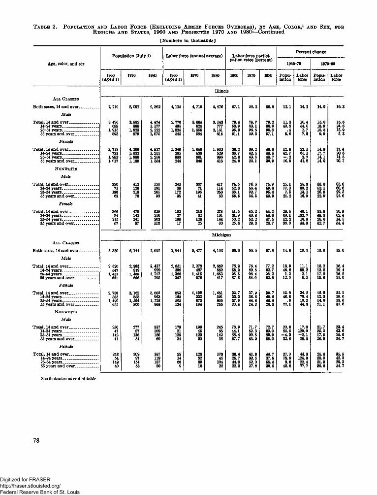
T a b l e 2 . P o p u l a t io n a n d L a b o r F o r c e (E x c l u d in g A r m e d F o r c e s O v e r s e a s ) , b y A g e , C o l o r ,1 a n d S e x , f o r R e g io n s a n d S t a t e s , 1960 a n d P r o je c t e d 1970 a n d 1980—Continued
[Numbers in thousands]
Age, color, and sexPopulation (July 1) Labor force (annual average) Labor force participation rates (percent)
Percent change1960-70 1970-80
1960(April 1) 1970 1980 1960(April 1) 1970 1980 1960 1970 1980 Population Laborforce Population LaborforceIllinois
A l l C l a s s e s
Both sexes, 14 and over.................. 7,219 8,092 9,302 4,125 4,710 5,476 57.1 58.2 58.9 12.1 14.2 14.9 16.3M a le
Total, 14 and over........................... 3,496 3,892 4,474 2,776 3,064 3,543 79.4 78.7 79.2 11.3 10.4 15.0 15.614-24 years................................. 688 990 1,177 405 624 777 58.9 63.1 66.0 43.8 54.0 18.9 24.625-54 years................................. 1,915 1,923 2,222 1,825 1,856 2,151 95.3 96.5 96.8 .4 1.7 15.5 15.955 years and over...................... 893 979 1,075 545 584 614 61.1 59.6 57.1 9.6 7.0 9.9 5.3F em ale
Total, 14 and over........................... 3,723 4,200 4.827 1,348 1,646 1,933 36.2 39.2 40.0 12.8 22.1 14.9 17.414 24 years................................. 723 1,032 1,215 265 438 529 36.7 42.5 43.5 42.7 65.1 17.7 20.625-54 years................................. 1,983r 1,980 2,258 839 861 986 42.3 43.5 43.7 - . 2 2.7 14.1 14.555 years and over...................... 1. 017 1,189 1,354 244 346 418 24.0 29.1 30.9 16.9 41.8 14.0 20.7N o n w h i t e
M a leTotal, 14 and over........................... 330 412 550 245 307 417 74.5 74.6 75.9 25.1 25.3 33.3 35.614-24 years................................. 71 126 191 38 71 114 52.8 56.4 59.6 77.0 89.2 52.1 60.625-54 years................................. 196 210 265 172 195 253 88.1 92.7 95.4 7.5 13.1 25.8 29.555 years and over...................... 63 76 93 35 41 50 56.5 54.5 53.9 21.2 16.9 22.9 21.6
F em aleTotal, 14 and over........................... 366 470 629 152 213 278 41.5 45.2 44.2 28.5 40.1 33.8 30.814-24 years................................. 84 142 210 27 62 101 31.9 43.8 48.0 69.1 132.7 48.3 62.425-54 years................................. 215 241 303 108 126 144 50.2 52.2 47.5 12.2 16.6 25.6 14.555 years and over..................... 67 87 116 17 25 33 25.6 28.3 28.7 30.0 44.0 32.7 34.4
MichiganAll Classes
Both sexes, 14 and over.................. 5,350 6,144 7,097 2,944 3,477 4,103 55.0 56.6 57.8 14.9 18.1 15.5 18.0M a le
Total, 14 and over........................... 2,620 2,983 3,437 2,051 2,278 2,652 78.3 76.4 77.2 13.9 11.1 15.2 16.414-24 years.................. - ........— 547 819 929 308 487 582 56.3 59.5 62.7 49.6 58.2 13.5 19.425-54 years________________ 1,451 1,468 1,717 1,386 1,415 1,653 95.5 96.4 96.2 1.2 2.1 17.0 16.855 years and over__________ 621 696 790 357 376 417 57.5 54.0 52.8 12.0 5.2 13.6 11.0F em a le
Total, 14 and over____ ________ 2,730 3,162 3,660 893 1,199 1,451 32.7 37.9 39.7 15.8 34.2 15.8 21.114-24 years................................ 585 858 963 195 332 391 33.3 38.6 40.6 46.6 70.4 12.3 18.025-54 years.-------- -------------- 1,490 1,504 1,728 565 673 805 37.9 44.8 46.6 .9 19.2 14.9 19.655 years and over.......... .......... 655 800 968 134 194 255 20.4 24.2 26.3 22.1 44.9 21.1 31.6N o n w h i t e
M a leTotal, 14 and over......................... 230 277 337 170 199 245 73.9 71.7 72.7 20.6 17.0 21.7 23.414-24 years___________ ____ 47 87 109 21 45 65 44.1 52.3 60.0 85.5 120.0 25.2 43.625-54 years........................ . 142 136 160 125 123 142 88.4 90.5 89.0 -4 .3 -2 .1 17.5 15.655 years and over......... ............ 41 54 69 24 30 38 57.7 55.9 55.0 32.6 28.5 26.8 24.7
F em aleTotal, 14 and over.......................... 243 309 387 88 128 173 36.4 41.3 44.7 27.0 44.3 25.3 35.514-24 years.................. ........... . 54 97 119 14 32 45 25.7 32.5 37.5 78.9 125.9 23.0 42.025-54 years........... .................. . 149 154 187 66 80 104 44.0 52.0 55.4 3.6 22.4 21.3 29.255 years and over______ ____ 40 58 80 9 16 25 22.3 27.6 30.5 43.6 77.7 39.8 54.7
See footnotes at end of table.
78
Digitized for FRASER http://fraser.stlouisfed.org/ Federal Reserve Bank of St. Louis
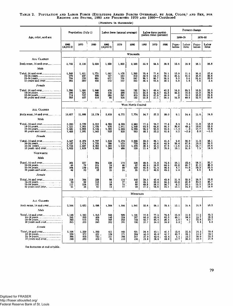
T a b l e 2 . P o p u l a t io n a n d L a b o r F o r c e (E x c l u d in g A r m e d F o r c e s O v e r s e a s ) , b y A g e , C o l o r ,1 a n d S e x , fo r R e g io n s a n d S t a t e s , 1960 a n d P r o je c t e d 1970 a n d 1980— Continued
[Numbers in thousands]
Population (July 1) Labor force (annual average) Labor force partici Percent changeAge, color, and sex pation rates (percent) 1960-70 1970-80
1960(April 1) 1970 1980 1960(April 1) 1970 1980 1960 1970 1980 Population Laborforce Population LaborforceWisconsin
All ClassesBoth sexes, 14 and over....... .......... 2,744 3,116 3,619 1,533 1,822 2,165 55.9 58.5 59.8 13.6 18.9 16.1 18.8
MaleTotal, 14 and over_____________ 1,348 1,521 1,771 1,057 1,178 1,383 78.4 77.4 78.1 12.9 11.5 16.4 17.414-24 years.................. ............ 279 407 473 167 260 314 59.9 64.0 66.5 45.6 55.6 16.3 20.825-54 years________________ 704 725 881 677 701 847 96.1 96.7 96.2 3.0 3.6 21.4 20.855 years and over__________ 364 390 418 213 217 222 58.4 55.6 53.1 6.9 1.8 7.3 2.4
FemaleTotal, 14 and over_____________ 1,396 1,595 1,848 476 644 782 34.1 40.4 42.3 14.2 35.2 15.9 21.514-24 years................................ 289 421 486 103 180 215 35.8 42.6 44.3 45.8 73.8 15.3 19.925-54 years........................ ....... 714 717 848 285 341 415 39.9 47.6 49.0 .3 19.5 18.3 21.855 years and over.................... 393 457 514 88 124 152 22.3 27.1 29.5 16.3 40.9 12.5 22.8
West North CentralAll Classes
Both sexes, 14 and over________ 10,827 11,808 13,179 5,919 6,772 7,774 54.7 57.3 59.0 9.1 14.4 11.6 14.8Male
Total, 14 and over_____________ 5,280 5,729 6,411 4,092 4,393 4,965 77.5 76.7 77.4 8.5 7.4 11.9 13.014-24 years________________ 1,121 1, 565 1,731 676 1,011 1,148 60.3 64.6 66.3 39.6 49.5 10.6 13.525-54 y e a r s . --------------- 2,691 2,663 3,134 2,562853 2,554 3,002 95.2 95.9 95.8 - 1.0 - . 3 17.7 17.655 years and over................ . 1,468 1,501 1,545 828 815 58.1 55.2 52.8 2.2 -2 .9 3.0 -1 .5Female
Total, 14 and over......... ................. 5,547 6,079 6,767 1,828 2,379 2,809 33.0 39.1 41.5 9.6 30.2 11.3 18.114-24 years________________ 1,137 1,574 1,731 399 670 778 35.1 42.6 44.9 38.4 67.8 10.0 16.225-54 years_______________ 2,758 2,687 3,081 1,059 1,223 1,473 38.4 45.5 47.8 - 2.6 15.5 14.7 20.455 years and over............ ....... 1,652 1,819 1,956 369 486 559 22.4 26.7 28.6 10.1 31.6 7.5 14.9N on white
MaleTotal, 14 and over......... ................. 201 237 304 138 170 226 68.6 71.8 74.3 18.1 23.6 28.2 32.714-24 years________________ 48 79 111 24 46 67 49.3 58.3 60.5 62.9 92.7 41.2 46.425-54 years.----------------------- 104 109 141 89 99 133 85.8 91.4 94.4 4.7 11.6 29.3 33.555 years and over___ ______ 49 50 53 25 25 26 51.0 49.9 49.5 2.4 .3 5.5 4.4
FemaleTotal, 14 and over_____________ 218 264 338 86 114 148 39.5 43.4 43.9 21.0 32.8 28.3 29.814-24 years________________ 50 82 115 14 27 40 28.1 33.0 34.5 63.6 92.3 40.5 46.725-54 years________________ 117 124 157 58 70 89 49.8 56.5 56.7 6.2 20.5 26.2 26.655 years and over__________ 51 58 67 14 17 20 27.2 29.9 30.1 13.1 24.3 15.5 16.3
MinnesotaAll Classes
Both sexes, 14 and over____ ____ 2,344 2,652 3,098 1,304 1,544 1,841 55.6 58.2 59.4 13.1 18.4 16.8 19.2Male
Total, 14 and over____________ 1,148 1,292 1,515 893 999 1,191 77.8 77.3 78.6 12.6 11.9 17.2 19.214-24 years________________ 241 353 408 145 224 267 60.0 63.6 65.5 46.1 54.9 15.7 19.325-54 years________________ 592 615 761 566 593 733 95.7 96.4 96.4 3.8 4.7 23.8 23.755 years and over..................... 315 325 346 182 182 190 57.7 56.0 54.9 3.3 .2 6.4 4.3Female
Total, 14 and over____________ 1,196 1,359 1,583 411 545 651 34.4 40.1 41.1 13.6 32.5 16.5 19.414-24 years_______________ 259 372 427 104 171 204 40.0 46.0 47.7 43.7 65.1 14.9 19.125-54 years_______________ 598 605 732 227 264 317 37.9 43.6 43.4 1.1 16.2 20.9 20.355 years and over_________ 340 383 424 81 110 130 23.8 28.8 30.6 12.7 36.6 10.9 17.6
See footnotes at end of table.
79
Digitized for FRASER http://fraser.stlouisfed.org/ Federal Reserve Bank of St. Louis
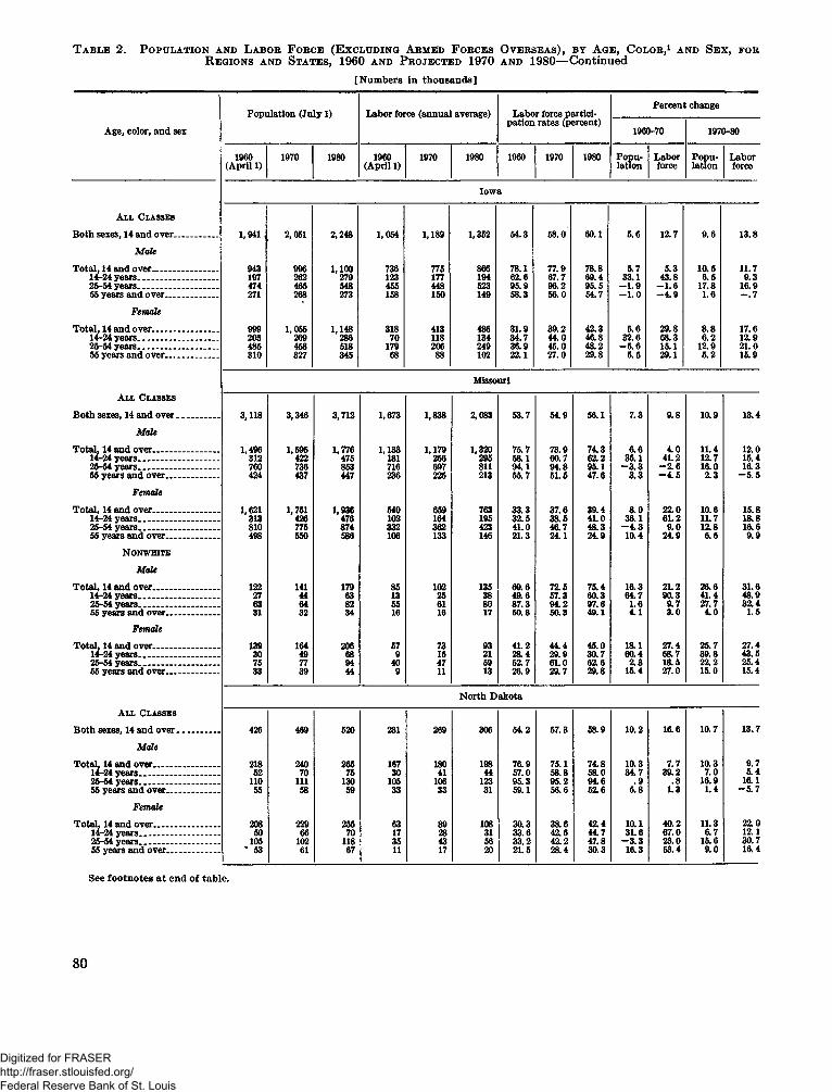
Table 2. Population and Labor Force (Excluding Armed Forces Overseas), by Age, Color,1 and Sex, for Regions and States, 1960 and Projected 1970 and 1980— Continued[Numbers in thousands]
Population (July 1) Labor force (annual average) Labor force partici Percent changeAge, color, and sex pation rates (percent) 1960-70 1970-80
1960(April 1) 1970 1980 1960(April 1) 1970 1980 1960 1970 1980 Population Laborforce Population LaborforceIowa
A l l C l a s s e s
Both sexes, 14 and over.................. 1,941 , 2,051 2,248 1,054 1,189 1,352 54.3 58.0 60.1 5.6 12.7 9.6 13.8M a le
Total, 14 and over........................... 943 996 1,100 736 775 866 78.1 77.9 78.8 5.7 5.3 10.5 11.714-24 years................................. 197 262 279 123 177 194 62.6 67.7 69.4 33.1 43.8 6.5 9.326-54 years............................. 474 465 548 455 448 523 95.9 96.2 95.5 -1 .9 - 1.6 17.8 16.955 years and over..................... 271 268 273 158 150 149 58.3 56.0 54.7 - 1.0 -4 .9 1.6 - . 7F em ale
Total, 14 and over........................... 999 1,055 1,148 318 413 486 31.9 39.2 42.3 5.6 29.8 8.8 17.614-24 years............................... . 203 269 286 70 118 134 34.7 44.0 46.8 32.6 68.3 6.2 12.925-54 years................................. 485 458 518 179 206 249 36.9 45.0 48.2 -5 .6 15.1 12.9 21.055 years and over...................... 310 327 345 68 88 102 22.1 27.0 29.8 5.5 29.1 5.2 15.9Missouri
A l l C l a s s e s
Both sexes, 14 and over.................. 3 ,1 1 8 3 ,3 4 6 3 ,7 1 2 1 ,6 7 3 1 ,8 3 8 2 ,0 8 3 5 3 .7 5 4 .9 5 6 .1 7 .3 9 .8 1 0 .9 1 3 .4M ale
Total, 14 and over........................... 1 ,4 9 6 1 ,5 9 5 1 ,7 7 6 1 ,1 3 3 1 ,1 7 9 1 ,3 2 0 7 5 .7 7 3 .9 7 4 .3 6 .6 4 .0 1 1 .4 1 2 .01 4 -2 4 years................................. 31 2 422 475 181 256 295 5 8 .1 6 0 .7 6 2 .2 3 5 .1 4 1 .2 1 2 .7 1 5 .42 5 -5 4 years................................. 760 736 853 716 697 811 9 4 .1 9 4 .8 9 5 .1 - 3 . 3 - 2 . 6 1 6 .0 1 6 .355 years and over...................... 424 437 447 236 225 213 5 5 .7 5 1 .5 4 7 .6 3 .3 - 4 . 5 2 .3 - 5 . 5
F em aleTotal, 14 and over........................... 1 ,6 2 1 1 ,7 5 1 1 ,9 3 6 540 659 763 3 3 .3 3 7 .6 3 9 .4 8 .0 2 2 .0 1 0 .6 1 5 .8
1 4 -2 4 years................................. 313 426 476 102 164 195 3 2 .5 3 8 .5 4 1 .0 3 6 .1 6 1 .2 1 1 .7 1 8 .82 5 -5 4 years................................. 810 775 87 4 3 3 2 362 423 4 1 .0 4 6 .7 4 8 .3 - 4 . 3 9 .0 1 2 .8 1 6 .655 years and over...................... 498 550 586 106 133 146 2 1 .3 2 4 .1 2 4 .9 1 0 .4 2 4 .9 6 .6 9 .9
N o n w h i t e
M aleTotal. 14 and over...........................
1 4 -2 4 years................................. 122 141 179 8 5 102 135 6 9 .6 7 2 .5 7 5 .4 1 6 .3 2 1 .2 2 6 .6 3 1 .627 4 4 63 13 25 38 4 9 .6 5 7 .3 6 0 .3 6 4 .7 9 0 .3 4 1 .4 4 8 .9
2 5 -5 4 years................................. 63 64 8 2 55 61 8 0 8 7 .3 9 4 .2 9 7 .6 1 .6 9 .7 2 7 .7 3 2 .455 years and over...................... 31 3 2 34 16 16 17 5 0 .8 5 0 .3 4 9 .1 4 .1 3 .0 4 .0 1 .5
F em aleTotal. 14 and over...........................
1 4 -2 4 years................................. 139 164 206 57 73 9 3 4 1 .2 4 4 .4 4 5 .0 1 8 .1 2 7 .4 2 5 .7 2 7 .430 49 68 9 15 21 2 8 .4 2 9 .9 3 0 .7 6 0 .4 6 8 .7 3 9 .8 4 3 .5
2 5 -5 4 years................................. 75 77 94 40 4 7 59 5 2 .7 6 1 .0 6 2 .6 2 .3 1 8 .5 2 2 .2 2 5 .455 years and over...................... 3 3 3 9 44 9 11 13 2 6 .9 2 9 .7 2 9 .8 1 5 .4 2 7 .0 1 5 .0 1 5 .4
North DakotaA l l C l a s s e s
Both sexes, 14 and over.................. 426 469 520 231 269 306 5 4 .2 5 7 .3 5 8 .9 1 0 .2 1 6 .6 1 0 .7 1 3 .7M ale
Total, 14 and over........................... 218 240 265 167 180 198 7 6 .9 7 5 .1 7 4 .8 1 0 .3 7 .7 1 0 .3 9 .71 4 -2 4 years................................. 52 70 75 3 0 41 44 5 7 .0 5 8 .8 5 8 .0 3 4 .7 3 9 .2 7 .0 5 .42 5 -5 4 years................................. 110 111 130 105 106 123 9 5 .3 9 5 .2 9 4 .6 . 9 . 8 1 6 .9 1 6 .155 years and over...................... 55 58 59 3 3 3 3 31 5 9 .1 5 6 .6 5 2 .6 5 .8 1 .3 1 .4 - 5 . 7
F em aleTotal, 14 and over........................... 208 229 255 63 8 9 108 3 0 .3 3 8 .6 4 2 .4 1 0 .1 4 0 .2 1 1 .3 2 2 .0
1 4 -2 4 years...................- ............ 50 66 70 17 28 31 3 3 .6 4 2 .6 4 4 .7 3 1 .6 6 7 .0 6 .7 1 2 .12 5 -5 4 years.....................- .......... 105 102 118 35 43 56 3 3 .2 4 2 .2 4 7 .8 - 3 . 3 2 3 .0 1 5 .6 3 0 .755 years and over______ ____ 0 53 61 67 11 17 20 2 1 .5 2 8 .4 3 0 .3 1 6 .3 5 3 .4 9 .0 1 6 .4
See footnotes at end of table.
8 0
Digitized for FRASER http://fraser.stlouisfed.org/ Federal Reserve Bank of St. Louis
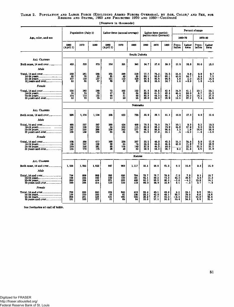
T a b l e 2 . P o p u l a t io n a n d L a b o r F o r c e (E x c l u d in g A r m e d F o r c e s O v e r s e a s ) , b y A g e , C o l o r ,1 a n d S e x , f o r R e g io n s a n d S t a t e s , 1960 a n d P r o je c t e d 1970 a n d 1980—Continued
[Numbers in thousands]
Age, color, and sexPopulation (July 1) Labor force (annual average) Labor force participation rates (percent)
Perceni1960-70
t change1970-80
1960(April 1) 1970 1980 1960(April 1) 1970 1980 1960 1970 1980 Population Laborforce Population LaborforceSouth Dakota
A l l C l a s s e s
Both sexes, 14 and over.................. 463 523 575 254 301 341 54.7 57.6 59.2 12.9 18.8 10.0 13.2M a le
Total, 14 and over........................... 233 261 286 181 199 218 77.7 76.5 76.3 11.6 9.9 9.9 9.714-24 years................................. 52 76 83 31 49 52 60.1 63.8 63.1 45.6 54.7 8.4 7.225-54 years................................. 117 119 137 111 113 129 95.4 95.6 94.8 1.9 2.0 15.3 14.455 years and over...................... 65 66 67 39 37 37 59.8 56.6 54.7 1.6 -3 .8 1.8 - 1.6
F em aleTotal, 14 and over........................... 230 263 289 72 102 122 31.5 38.8 42.4 14.3 41.1 10.1 20.114-24 years................................. 51 74 79 17 31 34 33.8 41.5 43.4 46.4 80.0 6.7 11.325-54 years................................. 114 115 132 40 51 65 35.3 44.0 49.1 1.0 26.0 14.1 27.555 years and over__r................. 65 73 78 15 20 23 23.0 28.0 29.9 12.6 37.2 7.4 14.9
NebraskaA l l C l a s s e s
Both sexes, 14 and over.................. 996 1,104 1,204 556 652 735 55.9 59.1 61.1 10.8 17.2 9.0 12.6
M a leTotal, 14 and over......... ................ 488 537 587 388 424 468 79.5 78.9 79.7 10.1 9.3 9.2 10.314-24 years................................. 102 148 162 64 102 115 62.8 68.5 70.9 44.8 57.9 9.0 12.925-54 years..........................— 247 250 286 238 242 277 96.2 96.8 96.6 1.2 1.8 14.6 14.455 years and over..................... 139 139 139 86 81 76 61.9 57.9 55.1 .4 - 6.2 - . 4 -5 .2
F em aleTotal, 14 and over........................... 506 566 617 168 228 267 33.2 40.3 43.3 11.5 35.5 8.9 17.014-24 years................................. 103 147 158 38 65 74 36.8 44.3 46.8 42.8 71.9 7.9 13.925-54 years................................. 250 250 281 95 116 140 37.8 46.3 50.0 22.3 12.2 21.255 years and over..................... 155 170 178 36 48 53 23.2 28.0 29.7 9.2 31.8 4.9 11.0
KansasA l l C l a s s e s
Both sexes, 14 and over.................. 1,538 1,665 1,822 847 980 1,117 55.1 58.8 61.3 8.2 15.6 9.5 14.0M a le
Total, 14 and over........................... 754 809 883 593 636 704 78.7 78.7 79.8 7.2 7.3 9.1 10.714-24 years...................... ......... 164 234 249 102 162 181 62.1 69.3 72.5 43.0 59.6 6.6 11.525-54 years................................. 390 368 419 371 355 405 95.2 96.3 96.5 —5.6 -4 .5 13.8 14.155 years and over..................... 200 206 214 120 120 119 60.0 58.0 55.6 3.1 - . 5 3.7 - . 5F em ale
Total, 14 and over........................... 784 856 940 254 343 412 32.4 40.1 43.9 9.1 35.1 9.8 2 a 114-24 years..............- ................. 159 220 235 52 92 106 32.5 42.0 45.1 38.7 79.0 6.6 14.625-54 years................................. 394 381 428 151 182 222 38.3 47.7 52.0 -3 .5 20.2 12.3 22.455 years and over................ . 231 255 277 51 69 84 22.3 27.2 30.3 10.4 34.6 8.9 21.4
See footnotes a t end of table.
81
Digitized for FRASER http://fraser.stlouisfed.org/ Federal Reserve Bank of St. Louis
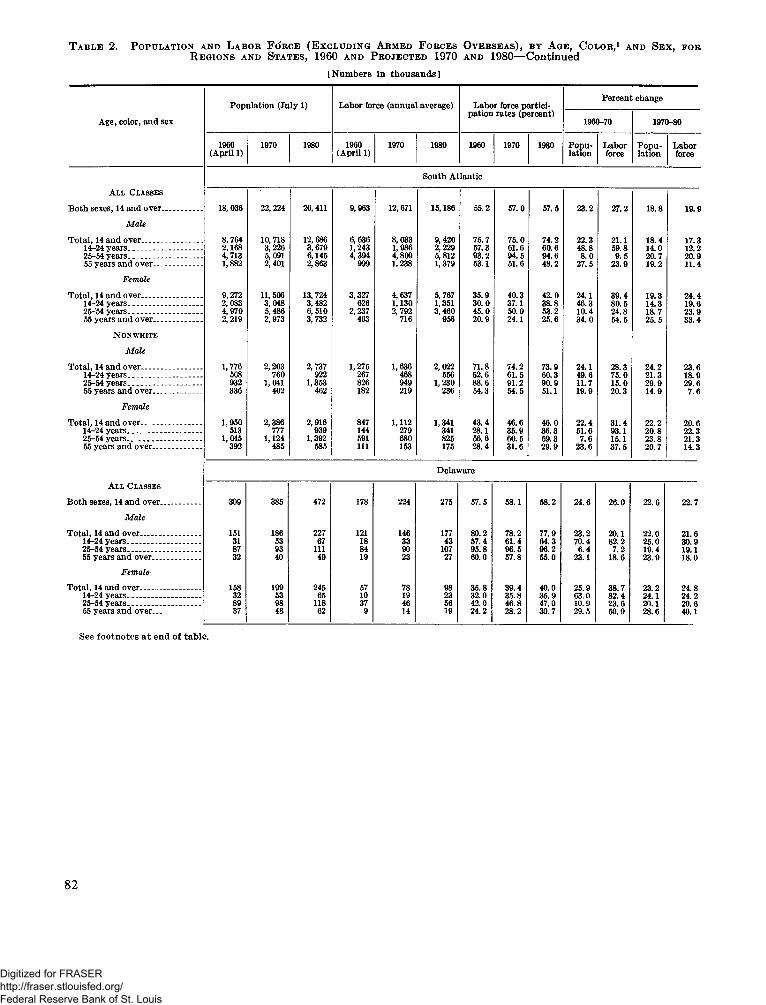
T a b l e 2 . P o p u l a t io n a n d L a b o r F o r c e (E x c l u d in g A r m e d F o r c e s O v e r s e a s ) , b y A g e , C o l o r ,1 a n d S e x , f o r R e g io n s a n d S t a t e s , 1960 a n d P r o je c t e d 1970 a n d 1980— Continued
[Numbers in thousands]
Age, color, and sexPopulation (July 1) Labor force (annual average) Labor force participation rates (percent)
Percent1960-70
; change1970-80
1960(April 1) 1970 1980 1960(April 1) 1970 1980 1960 1970 1980 Population Laborforce Population LaborforceSouth Atlantic
A l l C l a s s e s
Both sexes, 14 and over------------- 18, 036 22,224 26, 411 9,963 12, 671 15,186 55.2 57.0 57.5 23.2 27.2 18.8 19.9M a le
Total, 14 and over-------------------- 8, 764 10, 718 12,686 6,636 8, 033 9,420 75.7 75.0 74.2 22.3 21.1 18.4 17.314-24 years_______________ 2,168 3,226 3,679 1,243 1,986 2,229 57.3 61.6 60.6 48.8 59.8 14.0 12.226-54 years________________ 4,713 5,091 6,145 4,394 4, 809 5,812 93.2 94.5 94.6 8.0 9.5 20.7 20.955 years and over__________ 1, 882 2, 401 2,863 999 1,238 1,379 53.1 51.6 48.2 27.5 23.9 19.2 11.4F em ale
Total, 14 and over_____________ 9,272 11, 506 13, 724 3,327 4,637 5,767 35.9 40.3 42.0 24.1 39.4 19.3 24.414-24 years________________ 2,083 3, 048 3,482 626 1,130 1,351 30.0 37.1 38.8 46.3 80.5 14.3 19.625-*54 years._______________ 4,970 5, 486 6,510 2,237 2, 792 3,460 45.0 50.9 53.2 10.4 24.8 18.7 23.955 years and over__________ 2,219 2, 973 3,732 463 716 956 20.9 24.1 25.6 34.0 54.5 25.5 33.4N o n w h it e
M a leTotal, 14 and over_____________ 1, 776 2,203 2,737 1,275 1, 636 2, 022 71.8 74.2 73.9 24.1 28.3 24.2 23.614-24 ^ears________________ 508 760 922 267 468 556 52.6 61.5 60.3 49.6 75.0 21.3 18.925-54 years________________ 932 1,041 1,353 826 949 1,230 88.6 91.2 90.9 11.7 15.0 29.9 29.655 years and over__________ 336 402 462 182 219 236 54.3 54.5 51.1 19.9 20.3 14.9 7.6
F em aleTotal, 14 and over____________ 1,950 2,386 2,916 847 1,112 1,341 43.4 46.6 46.0 22.4 31.4 22.2 20.614-24 years________________ 513 777 939 144 279 341 28.1 35.9 36.3 51.6 93.1 20.8 22.325-54 years........................... . 1,045 1,124 1,392 591 680 825 56.6 60.5 59.3 7.6 15.1 23.8 21.355 years and over.............. . 392 485 585 111 153 175 28.4 31.6 29.9 23.6 37.5 20.7 14.3
DelawareA l l C la s s e s
Both sexes, 14 and over________ 309 385 472 178 224 275 57.5 58.1 58.2 24.6 26.0 22.6 22.7M a le
Total, 14 and over____________ 151 186 227 121 146 177 80.2 78.2 77.9 23.2 20.1 22.0 21.614-24 years________________ 31 53 67 18 33 43 57.4 61.4 64.3 70.4 82.2 25.0 30.925-54 years________________ 87 93 111 84 90 107 95.8 96.5 96.2 6.4 7.2 19.4 19.155 years and over__________ 32 40 49 19 23 27 60.0 57.8 55.0 23.1 18.6 23.9 18.0F em ale-
T o ta l , 14 and over_____________ 158 199 245 57 78 98 35.8 39.4 40.0 25.9 38.7 23.2 24.814-24 years------- ------------ 32 53 65 10 19 23 32.0 35.8 35.9 63.0 82.4 24.1 24.225-54 years________________ 89 98 118 37 46 56 42.0 46.8 47.0 10.9 23.6 20.1 20.655 years and over__________ 37 48 62 9 14 19 24.2 28.2 30.7 29.5 50.9 28.6 40.1
See footnotes at end of table.
8 2
Digitized for FRASER http://fraser.stlouisfed.org/ Federal Reserve Bank of St. Louis
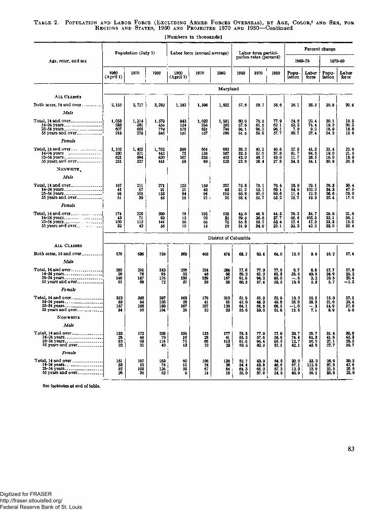
T a b l e 2 . P o p u l a t io n a n d L a b o r F o r c e ( E x c l u d in g A r m e d F o r c e s O v e r s e a s ) , b y A g e , C o l o r ,1 a n d S e x , f o r R e g io n s a n d S t a t e s , 1960 a n d P r o je c t e d 1970 a n d 1980— Continued
[Numbers in thousands]1
Population (July 1) Labor force (annual average) Labor force partici Percent changeAge, color, and sex pation rates (percent) 1960-70 1970-80
1960(April 1) 1970 1980 1960(April 1) 1970 1980 1960 1970 1980 Population Laborforce Population LaborforceMaryland
All ClassesBoth sexes, 14 and over...... .......... 2,155 2,717 3,282 1,242 1,596 1,922 57.6 58.7 58.6 26.1 28.5 20.8 20.4
M a leTotal, 14 and over........................... 1,053 1,314 1,579 843 1,032 1,231 80.0 78.5 77.9 24.8 22.4 20.1 19.314-24 years................................ 233 381 454 134 234 282 57.6 61.5 62.1 63.3 74.4 19.2 20.325-54 years........... ..................... 607 655 779 578 631 7r49 95.1 96.2 96.1 7.9 9.2 18.9 18.855 years and over................... . 213 278 346 131 167 199 61.5 59.9 57.7 30.7 27.4 24.2 19.6
F em aleTotal, 14 and over........................ . 1,102 1,402 1,703 399 564 692 36.2 40.2 40.6 27.3 41.3 21.4 22.614-24 years......................... ...... 230 371 442 75 138 167 32.5 37.0 37.8 61.7 84.5 19.0 21.525-54 years........... .................... 621 694 820 267 338 402 43.0 48.7 49.0 11.7 26.5 18.0 18.955 years and over....... ........... . 251 337 441 58 89 123 23.0 26.4 27.8 34.3 54.1 30.9 38.3
N on white % M a le
Total, 14 and over........................... 167 211 271 123 159 207 73.8 75.1 76.4 26.9 29.1 28.3 30.414-24 years................................ 41 67 91 21 43 63 51.2 63.1 69.1 64.0 102.2 34.3 47.025-54 years................ .............. 94 105 133 84 94 119 88.8 90.0 89.6 11.4 12.9 26.6 26.055 years and over..................... 31 39 48 18 22 25 58.4 55.7 53.2 25.2 19.3 22.4 17.0F em ale
Total, 14 and over....... .................. 174 225 290 78 106 128 45.0 46.9 44.3 29.3 34.7 28.9 21.614-24 years......... ...................... 43 71 93 13 26 35 29.5 36.6 37.7 65.6 105.3 32.1 36.125-54 years------------- ------ 100 112 141 56 65 75 55.8 58.2 53.4 12.4 17.3 25.3 15.055 years and over.............. ...... 32 42 56 10 14 18 31.9 34.0 32.1 33.3 42.2 33.0 25.4District of Columbia
All ClassesBoth sexes, 14 and over.................. 579 636 739 369 403 474 63.7 63.4 64.0 10.0 9.4 16.2 17.4
M a leTotal, 14 and over........................... 265 291 343 206 224 264 77.6 77.0 77.0 9.7 8.8 17.7 17.614-24 years................................. 56 76 95 33 46 58 59.2 61.2 61.3 35.6 40.0 24.9 25.225-54 years................................. 148 147 176 136 139 167 91.8 94.2 95.0 - . 5 2.2 19.5 20.455 years and over...................... 61 68 72 37 39 38 60.3 57.4 53.5 10.6 5.3 5.7 -1 .5
F em a leTotal, 14 and over........................... 313 345 397 163 179 210 51.9 51.9 52.9 10.2 10.1 15.0 17.114-24 years................................. 62 84 103 26 41 51 42.0 48.3 49.6 35.9 56.3 21.9 25.425-54 years................................. 167 166 190 107 107 126 64.1 64.6 66.1 - 1.0 - . 3 14.9 17.655 years and over...................... 84 95 104 29 32 33 35.0 33.0 31.8 13.5 7.1 8.9 5.0
N on white M a le
Total, 14 and over........................... 133 173 228 104 135 177 78.5 77.9 77.6 30.7 29.7 31.4 30.814-24 years................................ 28 49 70 16 28 41 55.3 57.5 58.9 74.4 81.3 41.8 45.325-54 years................................. 82 93 118 75 88 113 91.6 94.4 95.5 12.7 16.2 27.1 28.555 years and over..................... 22 31 40 13 19 23 59.3 60.9 57.1 42.1 45.9 27.7 19.7F em ale
Total, 14 and over........................... 151 197 253 80 106 138 52.7 53.9 54.5 30.2 33.2 28.9 30.314-24 years................................. 33 55 76 11 24 36 34.4 43.8 46.9 67.1 112.9 37.8 47.625-54 years................................. 92 103 126 59 67 84 64.3 65.2 67.3 12.3 13.9 21.5 25.555 years and over..................... 26 38 52 9 14 18 35.0 37.9 34.5 46.9 59.1 35.9 23.9
See footnotes at end of table.
83
Digitized for FRASER http://fraser.stlouisfed.org/ Federal Reserve Bank of St. Louis
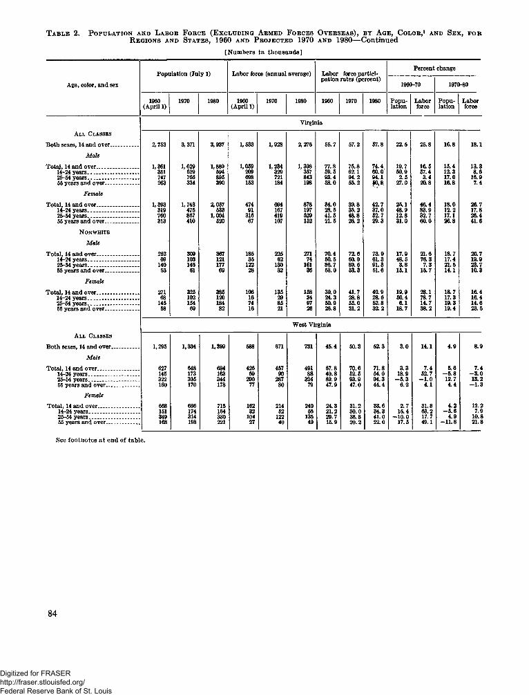
T a b l e 2 . P o p u l a t io n a n d L a b o r F o r c e (E x c l u d in g A r m ed F o r c e s O v e r s e a s ) , b y A g e , C o l o r ,1 a n d S e x , f o r R e g io n s a n d S t a t e s , 1960 a n d P r o je c t e d 1970 a n d 1980— Continued
[Numbers in thousands]
Age, color, and sexPopulation (July 1) Labor force (annual average) Labor force participation rates (percent)
Percent1960-70
change1970-80
1960(April 1) 1970 1980 1960(April 1) 1970 1980 1960 1970 1980 Population Laborforce Population LaborforceVirginia
All ClassesBoth sexes, 14 and over.................. 2,753 3,371 3,937 1,533 1,928 2,276 55.7 57.2 57.8 22.5 25.8 16.8 18.1
M a leTotal, 14 and over........................... 1,361 1,629 1,880 1,059 1,234 1,398 77.8 75.8 74.4 19.7 16.5 15.4 13.314-24 years— ........................... 351 529 594 209 329 357 59.5 62.1 60.0 50.9 57.4 12.3 8.625-54 years................................. 747 766 895 698 721 843 93.4 94.2 94.1 2.5 3.4 17.0 16.955 years and over...................... 263 334 390 153 184 198 58.0 55.2 27.0 20.8 16.8 7.4
F em aleTotal, 14 and over........................... 1,393 1,743 2,057 474 694 878 34.0 39.8 42.7 25.1 46.4 18.0 26.714-24 years................................. 319 475 533 91 167 197 28.5 35.2 37.0 48.9 83.9 12.2 17.825-54 years................................. 760 857 1,004 316 419 529 41.5 48.8 52.7 12.8 32.7 17.1 26.455 years and over..................... 313 410 520 67 107 152 21.5 26.2 29.3 31.0 60.0 26.8 41.6
N onwhiteM a le
Total, 14 and over........................... 262 309 367 185 225 271 70.4 72.6 73.9 17.9 21.6 18.7 20.714-24 years................................. 69 103 121 35 62 74 50.5 60.0 61.3 48.5 76.3 17.4 19.925-54 years................................. 140 146 177 122 130 161 86.7 89.6 91.3 3.8 7.3 21.5 23.755 years and over...................... 53 61 69 28 32 36 53.0 53.3 51.6 15.1 15.7 14.1 10.3F em ale
Total, 14 and over........................... 271 325 385 106 135 158 39.0 41.7 40.9 19.9 28.1 18.7 16.414-24 years................................. 68 102 120 16 29 34 24.3 28.8 28.6 50.4 78.7 17.3 16.425-54 years................................. 145 154 184 74 85 97 50.9 55.0 52.8 6.1 14.7 19.3 14.655 years and over....... ............. 58 69 82 16 21 26 26.8 31.2 32.2 18.7 38.2 19.4 23.5West Virginia
All ClassesBoth sexes, 14 and over________ 1,295 1,334 1,399 588 671 731 45.4 50.3 52.3 3.0 14.1 4.9 8.9
M a leTotal, 14 and over_____________ 627 648 684 426 457 491 67.8 70.6 71.8 3.3 7.4 5.6 7.414-24 years________________ 145 173 163 59 90 88 40.8 52.5 54.0 18.9 52.7 -5 .8 -3 .025-54 years______ _________ 322 305 344 290 287 324 89.9 93.9 94.3 -5 .3 - 1.0 12.7 13.255 years and over__________ 160 170 178 77 80 79 47.9 47.0 44.4 6.2 4.1 4.4 -1 .3
F em aleTotal, 14 and over_____________ 668 686 715 162 214 240 24.3 31.2 33.6 2.7 31.8 4.2 12.214-24 years________________ 151 174 164 32 52 56 21.2 30.0 34.3 15.4 63.2 -5 .6 7.925-54 years____ ___________ 349 314 330 104 122 135 29.7 38.8 41.0 - 10.0 17.7 4.9 10.855 years and over.............. ...... 168 198 221 27 40 49 15.9 20.2 22.0 17.5 49.1 - 11.8 21.8
See footnotes at end of table.
84
Digitized for FRASER http://fraser.stlouisfed.org/ Federal Reserve Bank of St. Louis
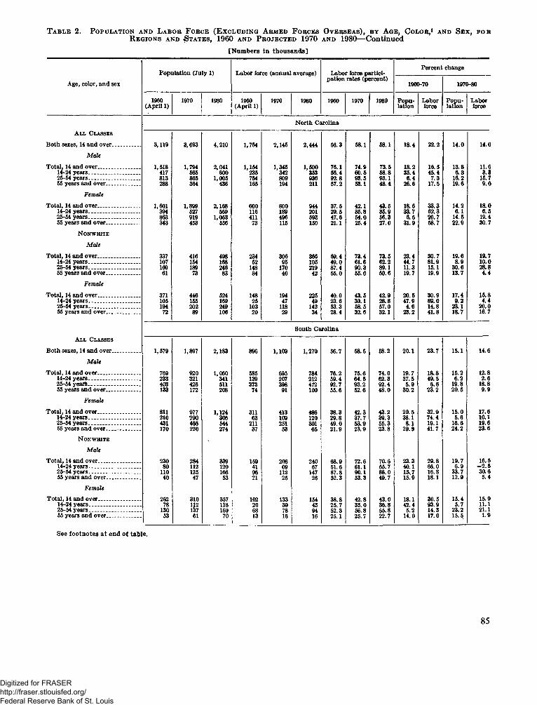
T a b l e 2 . P o p u l a t io n a n d L a b o r F o r c e ( E x c l u d in g A r m e d F o r c e s O v e r s e a s ) , b y A g e , C o l o r ,1 a n d S e x , f o r R e g io n s a n d S t a t e s , 1960 a n d P r o je c t e d 1970 a n d 1980— Continued
[Numbers in thousands]
Age, color, and sexPopulation (July 1) Labor force (annual average) Labor force participation rates (percent)
Percent change1960-70 1970-80
1960(April 1) 1970 1980 1960(April 1) 1970 1980 1960 1970 1980 Population Laborforce Population LaborforceNorth Carolina
All ClassesBoth sexes, 14 and over................ 3,119 3,693 4,210 1,754 2,145 2,444 56.3 58.1 58.1 18.4 22.2 14.0 14.0
M a leTotal, 14 and over........................... 1,518 1,794 2,041 1,154 1,345 1,500 76.1 74.9 73.5 18.2 16.5 13.8 11.614-24 years........... ......... ......... 417 565 600 235 342 353 56.4 60.5 58.8 35.4 45.4 6.3 3.325-54 years............................ 813 865 1,005 754 809 936 92.8 93.5 93.1 6.4 7.3 16.2 15.755 years and over..................... 288 364 436 165 194 211 57.2 53.1 48.4 26.6 17.5 19.6 9.0
F em aleTotal, 14 and over........................... 1,601 1,899 2,168 600 800 944 37.5 42.1 43.5 18.6 33.3 14.2 18.014-24 years................................ 394 527 559 116 189 201 29.5 35.8 35.9 33.7 62.3 6.1 6.525-54 years________________ 863 919 1,053 411 496 593 47.6 54.0 56.3 6.5 20.7 14.5 19.455 years and over................ . 343 453 556 73 115 150 21.1 25.4 27.0 31.9 58.7 22.9 30.7
NonwhiteM a le
Total, 14 and over..................... . 337 416 498 234 306 366 69.4 73.4 73.5 23.4 30.7 19.6 19.714-24 years...... .......................... 107 154 168 52 95 105 49.0 61.6 62.2 44.7 81.9 8.9 10.025-54 years................................ 169 189 246 148 170 219 87.4 90.3 89.1 11.3 15.1 30.6 28.855 years and over....... ............. 61 73 83 34 40 42 55.0 55.0 50.6 19.7 19.9 13.7 4.4F em ale
Total, 14 and over........................... 371 446 524 148 194 225 40.0 43.5 42.9 20.5 30.9 17.4 15.814-24 years................................ 105 155 169 25 47 49 23.6 30.1 28.8 47.9 89.0 9.2 4.425-54 years......................... ...... 194 202 249 103 118 142 53.3 58.5 57.0 4.6 14.8 23.1 20.055 years and over..................... 72 89 106 20 29 34 28.4 32.6 32.1 23.2 41.8 18.7 16.7
South CarolinaAll Classes
Both sexes, 14 and over.................. 1,579 1,897 2,183 896 1,109 1,270 56.7 58.5 58.2 20.1 23.7 15.1 14.6M a le
Total, 14 and over........................... 769 920 1,060 585 695 784 76.2 75.6 74.0 19.7 18.8 15.2 12.814-24 years................................. 233 321 341 139 207 212 59.4 64.5 62.3 37.5 49.5 6.2 2.625-54 yeart........................... 403 426 511 373 398 472 92.7 93.2 92.4 5.9 6.6 19.8 18.855 years and over....... .......... . 133 172 208 74 91 100 55.6 52.6 48.0 30.2 23.2 20.5 9.9F em ale
Total, 14 and over___ _________ 811 977 1,124 311 413 486 38.3 42.3 43.2 20.5 32.9 15.0 17.614-24 years................................ 210 290 306 63 109 120 29.8 37.7 39.3 38.1 74.4 5.6 10.125-54 years................................. 431 466 544 211 251 301 49.0 53.9 55.3 8.1 19.1 16.6 19.655 years and over...................... 170 220 274 37 53 65 21.9 23.9 23.8 29.9 41.7 24.2 23.6N on white
M a leTotal, 14 and over...................... 230 284 339 159 206 240 68.9 72.6 70.6 23.3 29.8 19.7 16.514-24 years................................ 80 112 120 41 69 67 51.6 61.1 55.7 40.1 66.0 6.9 -2 .525-54 years............................. . 110 125 166 96 112 147 87.8 90.1 88.0 13 7 16.8 33.7 30.655 years and over...................... 40 47 53 21 25 26 52.3 53.3 49.7 15.9 18.1 12.9 5.4
F em aleTotal, 14 and over....................... . 262 310 357 102 133 154 38.8 42.8 43.0 18.1 30.5 15.4 15.914-24 years........... .......... .......... 78 1J2 118 20 39 43 25.7 35.0 36.8 42.4 93.9 5.7 11.125-54 years...... ........ ........ ........ 130 137 169 68 78 94 52.3 56.8 55.8 5.2 14.3 23.2 21.155 years and over..................... 53 61 70 13 16 16 25.1 25.7 22.7 14.0 17.0 15.5 1.9
See footnotes a t end of table.
85
Digitized for FRASER http://fraser.stlouisfed.org/ Federal Reserve Bank of St. Louis
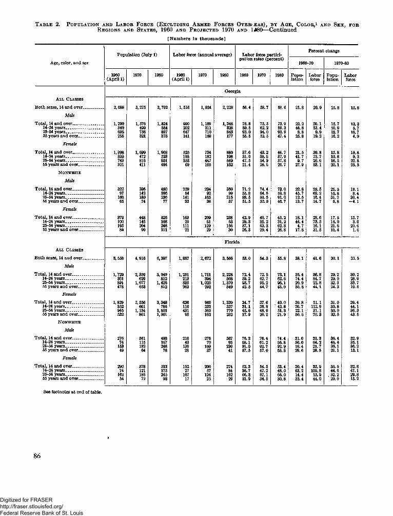
T a b l e 2 . P o p u l a t io n a n d L a b o r F o r c e (E x c l u d in g A r m e d F o r c e s O v e r s e a s ) , b y A g e , C o lo r ,1 a n d S e x , f o r R e g io n s a n d S t a t e s , 1960 a n d P r o je c t e d 1970 a n d 1*80— Continued
[Numbers in thousands]
Age, color, and sexPopulation (July 1) Labor force (annual average) Labor force participation rates (percent)
Percent1960-70
change1970-80
1960(April 1) 1970 1980 1960(April 1) 1970 1980 1960 1970 1980 Population Laborforce Population LaborforceGeorgia
All ClassesBoth sexes, 14 and over............ . 2,688 3,275 3,792 1,516 1,924 2,228 56.4 58.7 58.6 21.8 26.9 15.8 15.8
M aleTotal, 14 and over........................... 1,290 1,576 1,824 990 1,189 1,348 76.8 75.5 73.9 22.2 20.1 15.7 13.314-24 years........ ...................... . 340 499 554 202 311 328 59.5 62.2 59.3 46.8 53.4 10.9 5.726-54 years................. ............... 695 756 897 647 710 843 93.0 94.0 93.9 8.8 9.9 18.7 18.755 years and over...................... 255 321 373 141 169 177 55.5 52.5 47.4 25.8 19.2 16.2 4.9
F em aleTotal, 14 and over......................... . 1,398 1,699 1,968 525 734 880 37.6 43.2 44.7 21.5 39.8 15.8 19.814-24 years________________ 333 472 523 103 182 198 31.0 38.5 37.9 41.7 75.7 10.8 9.225-54 years_____ __________ 743 816 951 353 447 549 47.5 54.9 57.8 9.7 26.6 16.5 22.855 years and over.................. . 321 411 494 69 105 132 21.4 25.6 26.7 27.9 53.1 20.1 25.5
N on whiteM ale
Total, 14 and over______ _____ 322 395 480 229 294 350 71.2 74.4 73.0 22.8 28.5 21.5 19.114-24 years............. ........ .......... 97 142 166 54 92 99 55.8 64.5 59.8 45.7 68.2 16.8 8.425-54 years________________ 160 180 236 141 165 215 88.5 91.5 91.0 12.5 16.4 31.2 30.455 years and over..................... 65 74 77 33 38 37 51.5 52.0 46.7 13.7 14.7 6.8 -4 .1F em ale
Total, 14 and over....... .................. 379 448 526 163 209 238 42.9 46.7 45.2 18.1 28.6 17.5 13.714-24 years...................... .......... 100 145 168 29 51 53 29.3 35.2 31.2 44.4 73.5 16.0 3.025-54 years............. .......... ........ 195 204 248 111 129 156 57.1 63.3 62.8 4.7 16.1 21.6 20.655 years and over.................... 84 99 111 22 29 30 26.3 29.4 26.8 17.8 31.5 11.4 1.6
FloridaAll Classes
Both sexes, 14 and over............ . 3,558 4,916 6,397 1,887 2,672 3,566 53.0 54.3 55.8 38.1 41.6 30.1 33.5M ale
Total, 14 and over.......................... 1,729 2,359 3,049 1,251 1,711 2,228 72.4 72.5 73.1 36.4 36.8 29.2 30.214-24 years................................ 361 629 812 213 394 508 59.2 62.7 62.6 74.4 84.7 29.0 28.925-54 years................................ 891 1,077 1,425 835 1,025 1,370 93.7 95.2 96.1 20.9 22.8 32.3 33.755 years and over....... ............. 478 653 812 203 292 349 42.5 44.7 43.0 36.8 44.1 24.3 19.5F em ale
Total, 14 and over_____________ 1,829 2,556 3,348 636 960 1,339 34.7 37.6 40.0 39.8 51.1 31.0 39.414-24 years________________ 352 601 786 110 233 337 31.1 38.8 ' 42.8 70.7 112.9 30.8 44.125-54 years........................ ........ 945 1,154 1,501 431 565 770 45.6 48.9 51.3 22.1 31.1 30.0 36.355 years and over.............. ....... 532 801 1,061 95 162 232 17.9 20.2 21.9 50.6 70.3 32.5 43.5N onwhite
M aleTotal, 14 and over................... ....... 276 361 493 210 276 367 76.2 76.4 74.4 31.0 31.3 36.4 32.914-24 years________________ 74 115 167 43 70 95 58.1 61.2 56.8 56.0 64.2 45.4 35.124-54 years................................. 153 182 248 139 169 230 91.0 92.7 92.9 19.4 21.7 36.1 36.255 years and over................... 49 64 78 28 37 41 57.5 57.0 53.3 29.6 28.5 21.1 13.1
F em aleTotal, 14 and over........................... 290 378 513 152 206 274 52.3 54.5 53.4 30.4 35.9 35.5 32.814-24 years______ _________ 74 121 175 27 57 84 36.7 47.2 48.0 63.2 109.8 44.6 47.125-54 years........................... . 162 185 245 107 124 162 66.3 67.1 66.0 14.4 15.9 . 32.2 29.855 years and over................... 54 72 93 17 25 29 31.9 34.5 30.8 33.4 44.0 29.0 15.2
See footnotes at end of table.
8 6
Digitized for FRASER http://fraser.stlouisfed.org/ Federal Reserve Bank of St. Louis
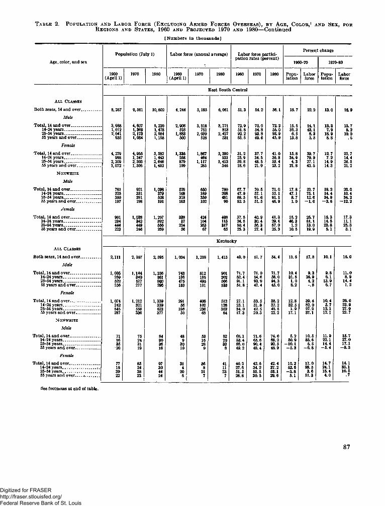
T a b l e 2. P o p u l a t io n a n d L a b o r F o r c e ( E x c l u d in g A r m ed F o r c e s O v e r s e a s ) , b y A g e , C o l o r ,1 a n d S e x , f o r R e g io n s a n d S t a t e s , 1960 a n d P r o je c t e d 1970 a n d 1980—Continued
[Numbers in thousands]
Age, color, and sexPopulation (July 1) Labor force (annual average) Labor force participation rates (percent)
Percent change1960-70 1970-80
I960(April 1) 1970 1980 1960(April 1) 1970 1980 1960 1970 1980 Population Laborforce Population LaborforceEast South Central
All ClassesBoth sexes, 14 and over.................. 8,267 9,561 10,802 4,244 5,185 6,061 51.3 54.2 56.1 15.7 22.2 13.0 16.9
M aleTotal, 14 and over....................... 3,988 4,607 5,220 2,908 3,318 3,771 72.9 72.0 72.2 15.5 14.1 13.3 13.714-24 years................................ 1,012 1,369 1,478 525 751 813 51.8 54.8 55.0 35.3 43.1 7.9 8.225-54 years........ ........................ 2,041 2,173 2,584 1,883 2,039 2,427 92.2 93.8 93.9 6.5 8.3 18.9 19.055 years and over...................... 935 1,064 1,158 500 528 531 53.5 49.6 45.9 13.8 5.5 8.8 .6
F em aleTotal, 14 and over..................... . 4,279 4,955 5,582 1,336 1,867 2,290 31.2 37.7 41.0 15.8 39.7 12.7 22.714-24 years________________ 998 1,347 1,443 258 464 531 25.9 34.5 36.8 34.9 79.9 7.2 14.425-54 years................................ 2,209 2,303 2,646 879 1,117 1,413 39.8 48.5 53.4 4.3 27.1 14.9 26.555 years and over..................... 1,072 1,305 1,492 199 285 346 18.6 21.9 23.2 21.8 43.5 14.3 21.2
N onwhiteM ale
Total, 14 and over....................... 781 921 1,098 529 650 780 67.7 70.5 71.0 17.8 22.7 19.2 20.014-24 years........ ........................ 225 331 379 108 189 208 47.9 57.1 55.1 47.1 75.1 14.4 10.425-54 years................. ........... . 360 391 528 318 359 481 88.5 91.6 91.1 8.7 12.6 34.9 34.255 years and over..................... 197 198 191 103 102 90 52.5 51.5 46.9 1.0 - 1.0 -3 .6 - 12.2
F em aleTotal, 14 and over........................... 901 1,038 1,207 338 424 498 37.5 40.9 41.3 15.2 25.7 16.3 17.314-24 years______ _________ 234 342 392 57 104 115 24.5 30.4 29.4 46.3 81.1 14.5 11.125-54 years...................... .......... 444 449 556 224 253 317 50.4 56.3 57.0 1.2 13.0 23.8 25.355 years and over................ . 223 246 259 56 67 65 25.3 27.4 25.3 10.5 19.9 5.1 3.1
KentuckyAll Classes
Both sexes, 14 and over.................. 2,111 2,357 2,595 1,034 1,218 1,413 49.0 51.7 54.4 11.6 17.8 10.1 16.0M a le
Total, 14 and over....... .................. 1,036 1,144 1,256 743 812 901 71.7 71.0 71.7 10.4 9.3 9.8 11.014-24 years................................. 259 340 361 136 186 202 52.4 54.6 56.0 31.5 36.9 6.1 8.925-54 years...... ................. ........ 522 527 600 475 495 566 91.1 93.9 94.3 1.0 4.2 13.9 14.455 years and over..................... 256 277 296 133 131 133 51.8 47.4 45.0 8.2 -.8 6.7 1.2
F em aleTotal, 14 and over....... ................ 1, 074 1,212 1,339 291 406 512 27.1 33.5 38.2 12.8 39.4 10.4 26.014-24 years................................. 242 321 339 56 102 126 23.1 31.8 37.2 32.5 82.0 5.7 23.925-54 years______ _________ 545 556 623 186 236 302 34.0 42.5 48.5 1.9 27.2 12.1 27.955 years and over...................... 287 336 377 50 68 84 17.3 20.3 22.2 17.1 37.1 12.1 22.7
N onwhiteM a le
Total, 14 and over........................... 71 75 84 48 53 62 68.1 71.6 74.0 5.2 10.5 11.9 15.714-24 years............................... 16 24 30 9 16 20 53.4 65.6 68.2 50.9 85.6 22.1 27.025-54 years............................. 35 31 36 30 28 33 86.0 90.4 92.5 - 10.1 5.5 14.4 17.155 years and over...................... 20 19 18 10 9 8 49.2 48.4 46.9 -5 .3 - 6.8 -5 .4 -8 .3F em ale
Total, 14 and over........................... 77 85 97 31 36 41 40.2 42.6 42.4 10.2 17.0 14.7 14.114-24 years............................. i . 16 24 30 4 8 11 27.6 34.2 37.2 52.6 88.5 24.1 35.125-54 years................................. 39 38 44 20 21 23 51.5 55.5 53.1 -3 .8 3.6 15.4 10.555 years and over___a............. 22 23 24 6 7 7 28.8 30.5 29.6 5.1 11.3 4.0 .7
See footnotes at end of table.
87
Digitized for FRASER http://fraser.stlouisfed.org/ Federal Reserve Bank of St. Louis

T a b l e 2 . P o p u l a t io n a n d L a b o r F o r c e (E x c l u d in g A r m e d F o r c e s O v e r s e a s ) , b y A g e , C o l o r ,1 a n d S e x , f o r R e g io n s a n d S t a t e s , 1960 a n d P r o je c t e d 1970 a n d 1980— Continued
[Numbers in thousands]
Age, color, and sexPopulation (July 1) Labor force (annual average) Labor force participation rates (percent)
Percent change1960-70 1970-80
1960(April 1) 1970 1980 1960(April 1) 1970 1980 1960 1970 1980 Population Laborforce Population LaborforceTennessee
All ClassesBoth sexes, 14 and over____ ____ 2,499 2,929 3,287 1,314 1,617 1,860 52.6 55.2 56.6 17.2 23.1 12.2 15.0
M a leTotal, 14 and over_____________ 1,199 1,407* 1,587 887 1,016 1,143 74.0 72.2 72.0 17.4 14.5 12.8 12.514-24 years________________ 293 400 427 153 215 232 52.4 53.8 54.3 36.5 39.9 6.9 7.925-54 years....................... ........ 630 682 797 583 637 743 92.5 93.4 93.2 8.2 9.2 16.9 16.755 years and over................ . 275 325 362 150 164 168 54.6 50.4 46.3 18.0 8.9 11.4 2.4
F em aleTotal, 14 and over_____________ 1,300 1,522 1,700 427 601 717 32.8 39.5 42.2 17.0 41.0 11.7 19.314-24 years________________ 295 399 422 82 147 160 27.8 36.8 38.0 35.5 79.3 5.6 9.125-54 years________________ 685 720 809 283 362 442 41.3 50.3 54.6 5.1 27.8 12.4 22.055 years and over...................... 321 402 469 61 92 115 19.2 23.0 24.6 25.4 50.3 16.4 24.7
N onwhiteM a le
Total, 14 and over....... ................... 176 211 253 122 143 170 69.2 68.1 67.2 19.6 17.8 20.2 18.614-24 years........................ ........ 45 71 85 21 39 45 48.1 54.4 52.9 59.8 80.7 19.9 16.725-54 years................................ 88 92 120 77 82 104 88.1 88.4 86.4 5.5 5.7 30.3 27.355 years and over...................... 44 47 47 23 23 21 52.8 49.2 44.4 7.0 - .1 .7 -9 .2F em ale
Total, 14 and over.............. ........... 202 240 283 82 103 119 40.8 42.8 42.1 18.7 24.6 18.0 15.914-24 years................................ 47 75 90 12 23 29 25.3 31.2 32.0 58.4 95.2 19.8 22.825-54 years................................ 106 107 130 57 62 72 53.6 57.8 55.8 1.0 9.0 21.7 17.755 years and over...................... 49 58 63 14 18 18 28.3 30.5 28.1 18.1 27.4 8.9 .4Alabama
All ClassesBoth sexes, 14 and over.................. 2,218 2,580 2,980 1,153 1,415 1,684 52.0 54.8 56.5 16.3 22.7 15.5 19.1
M aleTotal, 14 and over....... .................. 1,060 1,239 1,440 779 898 1,042 73.6 72.5 72.4 16.9 15.2 16.3 16.114 24 years............. .................. 270 365 400 139 200 214 51.4 54.7 53.3 35.3 43.9 9.6 6.925-54 years............................... 556 598 731 516 561 686 92.8 93.8 93.8 7.6 8.6 22.3 22.455 years and over__________ 234 275 309 125 138 143 53.3 50.0 46.2 17.8 10.4 12.1 3.6
F em aleTotal. 14 and over........................... 1,158 1,341 1,540 373 517 642 32.2 38.5 41.7 15.8 38.4 14.8 24.214-24 years________________ 277 369 401 73 128 147 26.4 34.8 36.6 33.0 75.0 8.7 14.425-54 years.................. .............. 607 631 739 250 313 403 41.1 49.6 54.5 3.9 25.3 17.2 28.955 years and over..................... 273 341 400 50 76 92 18.5 22.2 23.1 25.1 50.1 17.0 21.8
N onwhiteM ale
Total. 14 and over....... ................ 280 333 400 188 231 276 67.2 69.5 68.9 19.1 23.2 20.2 19.314-24 years........ ........................ 83 120 135 40 65 65 47.5 54.0 48.4 43.2 63.0 12.9 1.225-54 years................................ 130 145 197 115 132 179 88.0 90.9 90.7 11.4 15.0 35.9 35.555 years and over..................... 66 69 69 34 35 32 50.9 51.0 46.7 4.0 4.1 - .1 - 8.6
F em aleTotal, 14 and over........................... 329 375 434 124 155 180 37.5 41.3 41.4 13.9 25.5 15.8 16.114-24 years................................. 88 124 139 22 38 40 25.0 30.6 28.6 40.8 72.3 12.0 4.625-54 years................................. 163 164 202 83 94 118 50.7 57.2 58.3 .7 13.7 23.1 25.455 years and over___ ______ 78 87 93 19 23 23 24.2 26.7 24.1 11.3 22.7 7.2 -3 .1
See footnotes at end of table.
8 8
Digitized for FRASER http://fraser.stlouisfed.org/ Federal Reserve Bank of St. Louis
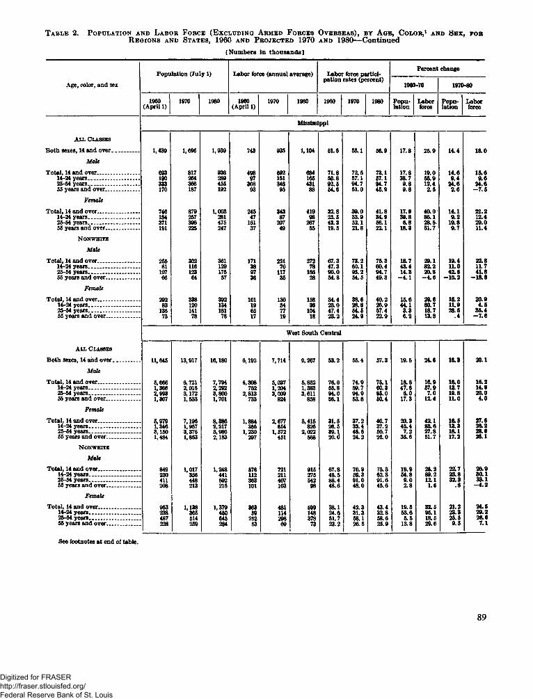
T a b l e 2 . P o p u l a t i o n a n d L a b o r F o r c e ( E x c l u d i n g A r m e d F o r c e s O v e r s e a s ) , b y A g e , C o l o r , 1 a n d S e x , f o r R e g i o n s a n d S t a t e s , 1960 a n d P r o j e c t e d 1970 a n d 1980—Continued
[Numbers in thousands]
Age, color, and sexPopulation (July 1) Labor force (annual average) Labor force participation rates (percent)
Percent change1960-70 1970-80
1960(April 1) 1970 1980 1960(April 1) 1970 1980 1960 1970 1980 Population Laborforce Population LaborforceMississippi
A l l C l a s s e s
Both sexes, 14 and over................. 1,439 1,696 1,939 743 935 1,104 51.6 55.1 56.9 17.8 25.9 14.4 18.0M ale
Total, 14 and over........................... 693 817 936 498 592 684 71.8 72.5 73.1 17.8 19.0 14.6 15.614-24 years................................. 190 264 289 97 151 165 50.8 57.1 57.1 38.7 55.9 9.4 9.625-54 years................................. 333 366 455 308 346 431 92.5 94.7 94.7 9.8 12.4 24.6 24.655 years and over...................... 170 187 192 93 95 88 54.6 51.0 45.9 9.8 2.5 2.6 -7 .5F em ale
Total, 14 and over........................... 746 879 1,003 245 343 419 32.8 39.0 41.8 17.9 40.0 14.1 22.214-24 years................................. 184 257 281 47 87 98 25.5 33.9 34.9 39.8 86.1 9.2 12.425-54 years................................. 371 396 475 161 207 267 43.3 52.1 56.1 6.8 28.5 19.8 29.055 years and over.............. — 191 225 247 37 49 55 19.5 21.8 22.1 18.3 31.7 9.7 11.4N o n w h i t e
M aleTotal, 14 and over........................... 255 302 361 171 221 272 67.3 73.2 75.3 18.7 29.1 19.4 22.814-24 years................................. 81 116 129 38 70 78 47.3 60.1 60.4 43.4 82.2 11.0 11.725-54 years................................. 107 123 175 97 117 166 90.0 95.2 94.7 14.3 20.8 42.5 41.855 years and over...................... 66 64 57 36 35 28 54.8 54.5 49.3 -4 .1 -4 .6 -10 .2 -18 .8
F em aleTotal, 14 and over........................... 292 338 392 101 130 158 34.4 38.6 40.2 15.6 29.6 16.2 20.914-24 years................................. 83 120 134 19 34 36 23.0 28.8 26.9 44.1 80.7 11.9 4.525-54 years................................. 136 141 181 65 77 104 47.4 54.5 57.4 3.3 18.7 28.5 35.455 years and over..................... 73 78 78 17 19 18 23.2 24.9 22.9 6.2 13.8 .4 -7 .6
West South CentralA l l C l a s s e s
Both sexes, 14 and over.................. 11,645 13,917 16,180 6,192 7,714 9,267 53.2 55.4 57.3 19.5 24.6 16.3 20.1M ale
Total, 14 and over........................... 5,666 6,721 7,794 4,308 5,037 5,852 76.0 74.9 75.1 18.6 16.9 16.0 16.214-24 years................................. 1,366 2,016 2,292 762 1,204 1,383 55.8 59.7 60.3 47.6 57.9 13.7 14.925-54 years................................. 2,993 3,172 3,800 2,813 3,009 3,611 94.0 94.9 95.0 6.0 7.0 19.8 20.055 years and over...................... 1,307 1,533 1,701 733 824 858 56.1 53.8 50.4 17.3 12.4 11.0 4.0F em ale
Total, 14 and over........................... 5,979 7,196 8,386 1,884 2,677 3,415 31.5 37.2 40.7 20.3 42.1 1 6 -5 27.614-24 years................................. 1,346 1,957 2,217 356 654 826 28.5 33.4 37.2 45.4 83.6 13.3 26.225-54 years................................. 3,150 3,375 3,986 1,230 1,572 2,022 39.1 46.6 50.7 7.2 27.8 18.1 28.655 years and over..................... 1,484 1,863 2,183 297 451 568 20. d 24.2 26.0 35.6 51.7 17.2 26.1N o n w h i t e
M aleTotal, 14 and over........................... 849 1,017 1,248 576 721 915 67.8 70.9 73.3 19.9 25.2 22.7 26.914-24 years................................. 230 356 441 112 211 275 48.5 59.3 62.3 54.8 89.2 23.8 30.125-54 years................................. 411 448 592 363 407 542 88.4 91.0 91.6 9.0 12.1 32.3 33.155 years and over...................... 208 213 215 101 103 98 48.6 48.0 45.6 2.8 1.5 .8 -4 .2
F em aleTotal, 14 and over........................... 953 1,138 1,379 363 481 599 38.1 42.3 43.4 19.5 32.5 21.2 24.614-24 years................................. 238 365 450 59 114 148 24.6 31.3 32.8 53.6 95.1 23.3 29.225-54 years................................. 487 514 645 252 298 378 51.7 58.1 58.6 5.5 18.5 25.5 26.655 years and over...................... 228 259 284 53 69 73 23.2 26.5 25.9 13.8 29.6 9.5 7.1
See footnotes at end of table.
89
Digitized for FRASER http://fraser.stlouisfed.org/ Federal Reserve Bank of St. Louis
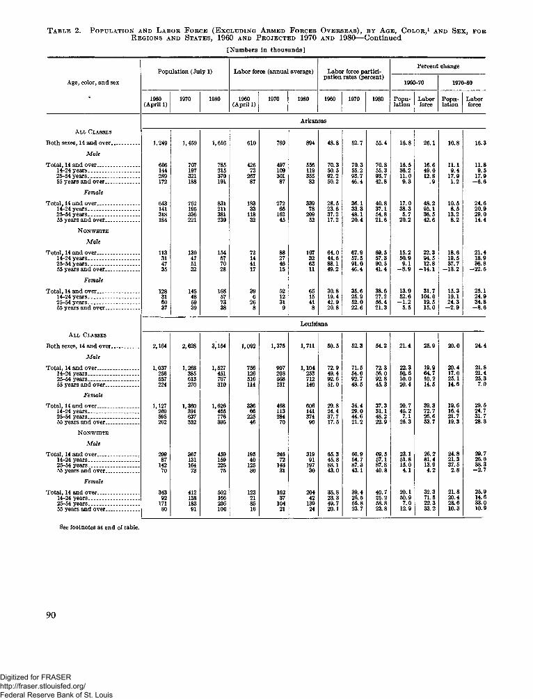
T a b l e 2 . P o p u l a t i o n a n d L a b o r F o r c e ( E x c l u d i n g A r m e d F o r c e s O v e r s e a s ) , b y A g e , C o l o r , 1 a n d S e x , f o r R e g i o n s a n d S t a t e s , 1960 a n d P r o j e c t e d 1970 a n d 1980— Continued
[Numbers in thousands]
Age, color, and sexPopulation (July 1) Labor force (annual average) Labor force participation rates (percent)
Percent1960-70
change1970-80
1960(April 1) 1970 1980 1960(April 1) 1970 1980 1960 1970 1980 Population Laborforce Population LaborforceArkansas
A l l C l a s s e s
Both sexes, 14 and over............ 1,249 1,459 1,616 610 769 894 48.8 52.7 55.4 16.8 26.1 10.8 16.3Male
Total, 14 and over_____________ 606 707 785 426 497 556 70.3 70.3 70.8 16.5 16.6 11.1 11.814-24 years________________ 144 197 215 73 109 119 50.5 55.2 55.3 36.2 49.0 9.4 9.525-54 years________________ 289 321 379 267 301 355 92.2 93.7 93.7 11.0 12.8 17.9 17.955 years and over__________ 172 188 191 87 87 82 50.2 46.4 42.8 9.3 .9 1.2 -6 .6Female
Total, 14 and over_____________ 643 752 831 183 272 339 28.5 36.1 40.8 17.0 48.2 10.5 24.614-24 years_____________ 141 195 211 33 65 78 23.6 33.3 37.1 38.3 95.1 8.5 20.925-54 years_____ ________ 318 336 381 118 162 209 37.2 48.1 54.8 5.7 36.5 13.2 29.055 years and over________ 184 221 239 32 45 52 17.2 20.4 21.6 20.2 42.6 8.2 14.4N o n w h i t e
MaleTotal, 14 and over_____________ 113 130 154 72 88 107 64.0 67.9 69.5 15.2 22.3 18.6 21.414-24 years_______ ______ 31 47 57 14 27 32 44.6 57.5 57.3 50.9 94.5 19.5 18.925-54 years________________ 47 51 70 41 46 63 88.1 91.0 90.5 9.1 12.8 37.7 36.855 years and over__________ 35 32 28 17 15 11 49.2 46.4 41.4 -8 .9 -14.1 -13.2 -22 .5
FemaleTotal, 14 and over_____________ 128 145 168 39 52 65 30.8 35.6 38.6 13.9 31.7 15.3 25.114-24 years________________ 31 48 57 6 12 15 19.4 25.9 27.2 52.6 104.0 19.1 24.925-54 years________________ 60 59 73 26 31 41 42.9 52.0 56.4 -1 .2 19.5 24.3 34.855 years and over__________ 37 39 38 8 9 8 20.8 22.6 21.3 5.5 15.0 -2 .9 -8 .6
LouisianaA l l C l a s s e s
Both sexes, 14 and over............ . 2,164 2,628 3,154 1,092 1,375 1,711 50.5 52.3 54.2 21.4 25.9 20.0 24.4Male
Total, 14 and over.......................... 1,037 1,268 1,527 756 907 1,104 72.9 71.5 72.3 22.3 19.9 20.4 21.814-24 years________________ 256 385 451 126 208 253 49.4 54.0 56.0 5Q.6 64.7 17.0 21.425-54 years________________ 557 613 767 516 568 712 92.6 92.7 92.8 10.0 10.2 25.1 25.355 years and over______ ____ 224 270 310 114 131 140 51.0 48.5 45.3 20.4 14.5 14.6 7.0Female
Total, 14 and over____________ 1,127 1,360 1,626 336 468 606 29.8 34.4 37.3 20.7 39.3 19.6 29.514-24 years________________ 269 391 455 66 113 141 24.4 29.0 31.1 45.2 72.7 16.4 24.725-54 years____________ . . . 595 637 776 225 284 374 37.7 44.6 48.2 7.1 26.6 21.7 31.755 years and over.................... 262 332 395 46 70 90 17.5 21.2 22.9 26.3 53.7 19.3 28.3N o n w h i t e
MaleTotal, 14 and over....... ................... 299 367 459 195 246 319 65.3 66.9 69.5 23.1 26.2 24.8 29.714-24 years_______________1 87 131 159 40 72 91 45.8 54.7 57.1 51.8 81.4 21.3 26.625-54 years________________ 142 164 225 125 143 197 88.1 87.3 87.8 15.0 13.9 37.5 38.355 years and over__________ 70 73 75 30 31 30 43.0 43.1 40.8 4.1 4.2 2.8 -2 .7
FemaleTotal, 14 and over........................ 343 412 502 123 162 204 35.8 39.4 40.7 20.1 32.3 21.8 25.914-24 years________________ 92 138 166 21 37 42 23.3 26.5 25.2 50.9 71.5 20.4 14.625-54 years________ _______ 171 183 236 85 104 139 49.7 56.8 58.8 7.0 22.3 28.6 33.055 years and over..................... 80 91 100 16 21 24 20.1 23.7 23.8 12.9 33.2 10.3 10.9
See footnotes at end of table.
90
Digitized for FRASER http://fraser.stlouisfed.org/ Federal Reserve Bank of St. Louis
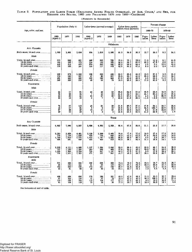
T a b l e 2. P o p u l a t io n a n d L a b o r F o r c e (E x c l u d in g A r m e d F o r c e s O v e r s e a s ) , b y A g e , C o l o r ,1 a n d S e x , f o r R e g io n s a n d S t a t e s , 1960 a n d P r o je c t e d 1970 a n d 1980—Continued
[Numbers in thousands]
Population (July 1) Labor force (annual average) Labor force partici Percent changeAge, color, and sex pation rates (percent) 1960-70 1970-80
1960(April 1) 1970 1980 1960(April 1) 1970 1980 1960 1970 1980 Population Laborforoe Population LaborforceOklahoma
A l l C l a s s e s
Both sexes, 14 and over................. 1,668 1,881 2,054 854 1,016 1,160 51.2 54.0 56.5 12.7 19.0 9.2 14.1Male
Total, 14 and over......................... 812 908 991 596 663 732 73.5 73.1 73.8 11.8 11.2 9.1 10.314-24 years____ ___________ 190 256 273 104 153 168 54.8 59.7 61.6 35.3 47.3 6.6 10.125-54 years________________ 406 418 476 379 393 450 93.2 94.0 94.4 2.9 3.8 13.9 14.455 years and over__________ 216 233 241 114 117 113 52.8 50.2 47.0 8.0 2.8 3.4 -3 .2Female
Total, 14 and over....... ................... 856 973 1,063 258 353 428 30.1 36.3 40.3 13.6 37.1 9.3 21.214-24 years________________ 179 242 257 47 86 107 26.3 35.7 41.8 35.2 83.6 6.3 24.125-54 years------------------------ 431 442 490 162 198 242 37.6 45.0 49.3 2.5 22.5 11.0 21.555 years and over__________ 246 289 316 48 68 79 19.6 23.5 25.1 17.3 40.8 9.2 16.8N o n w h i t e
MaleTotal, 14 and over............. ............. 66 77 91 40 49 62 60.5 64.0 67.4 16.2 23.0 18.9 25.214-24 years______________ 18 28 34 7 15 19 41.3 52.7 56.1 54.1 96.5 21.5 29.425-54 years________________ 30 32 41 25 27 36 82.5 86.6 87.8 4.2 9.3 30.5 32.355 years and over__________ 18 18 16 8 7 7 42.4 41.3 39.5 -1 .4 -3 .9 -5 .9 -10 .0
FemaleTotal, 14 and over_____________ 74 87 103 23 31 39 31.6 36.0 37.4 17.6 34.1 18.7 23.414-24 years________________ 18 27 34 4 9 13 20.9 32.1 37.3 54.0 136.7 23.6 43.425-54 years________________ 37 38 46 16 17 21 42.5 46.0 44.8 3.4 11.9 22.9 19.7
55 years and over__________ 19 22 23 4 5 5 20.8 23.5 22.6 11.3 25.6 5.3 1.6
TexasA l l C l a s s e s
Both sexes, 14 and over....... .......... 6,563 7,949 9,357 3,636 4,553 5,503 55.4 57.3 58.8 21.1 25.2 17.7 20.8Male
Total, 14 and over___ _________ 3, 210 3,839 4,491 2,529 2,969 3,460 78.8 77.4 77.0 19.6 17.4 17.0 16.514-24 years________________ 776 1,178 1,353 459 734 843 59.2 62.3 62.3 51.8 59.8 14.9 14.925-54 years________________ 1,740 1,820 2,178 1,652 1,747 2,095 94.9 96.0 96.2 4.6 5.8 19.7 19.955 years and over__________ 694 841 960 418 489 523 60.2 58.1 54.4 21.1 16.8 14.1 6.9
FemaleTotal, 14 and over_____________ 3,353 4,111 4,866 1,107 1,584 2,043 33.0 38.5 42.0 22.6 43.1 18.4 29.014-24 years________________ 757 1,130 1,295 210 399 499 27.8 34.5 38.5 49.3 85.1 14.6 28.025-54 years________________ 1,805 1,960 2,339 725 927 1,197 40.2 47.3 51.2 8.6 27.9 19.4 29.155 years and over__________ 791 1,021 1,232 171 267 347 21.7 26. 2 28.2 29.1 55.9 20.7 29.8
N o n w h i t e Male
Total, 14 and over_____________ 371 443 544 269 338 428 72.4 76.2 78.6 19.4 25.7 22.8 26.714-24 years________________ 94 150 191 51 98 132 53.7 65.1 69.3 59.0 92.8 27.7 35.825-54 years________________ 192 202 256 172 191 246 89.7 94.6 95.8 5.3 11.1 27.0 28.555 years and over__________ 85 91 96 46 49 50 54.1 53.7 51.5 7.3 6.4 5.3 1.1
FemaleTotal, 14 and over....... ............... 408 494 606 178 236 291 43.6 47.8 48.1 21.0 32.5 22.7 23.414-24 years________________ 97 152 193 27 57 78 28.2 37.2 40.2 56.3 106.0 27.2 37.425-54 years_____ __________ 219 234 289 125 146 177 57.2 62.5 61.2 6.5 16.5 23.8 21.2
55 years and over__________ 91 108 123 25 33 36 27.5 30.7 29.5 18.4 32.3 Hi 1 9.6See footnotes at end of table.
91
Digitized for FRASER http://fraser.stlouisfed.org/ Federal Reserve Bank of St. Louis
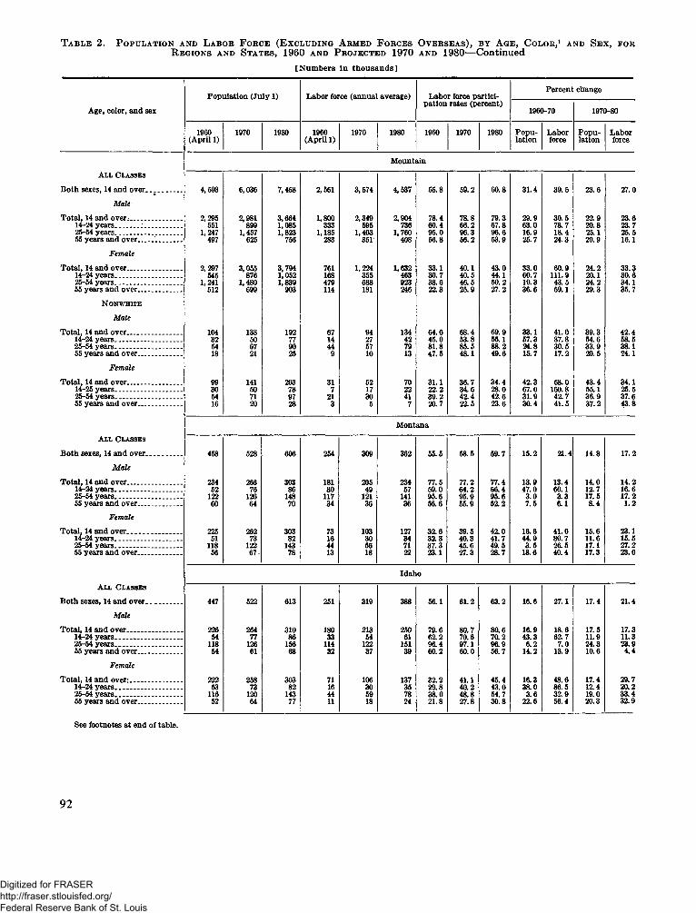
T a b l e 2 . P o p u l a t i o n a n d L a b o r F o r c e ( E x c l u d i n g A r m e d F o r c e s O v e r s e a s ) , b y A g e , C o l o r , 1 a n d S e x , f o r R e g i o n s a n d S t a t e s , 1 9 6 0 a n d P r o j e c t e d 1 9 7 0 a n d 1 9 8 0 — Continued
[Numbers in thousands]
Population (July 1) Labor force (annual average) Labor force partici Percent changeAge, color, and sex pation rates (percent) 1960-70 1970-80
1960(April 1) 1970 1980 1960(April 1) 1970 1980 1960 1970 1980 Population Laborforce Population LaborforceMountain
A l l C l a s s e s
Both sexes, 14 and over.................. 4,593 6,036 7,458 2,561 3,574 4,537 55.8 59.2 60.8 31.4 39.5 23.6 27.0Male
Total, 14 and over.:................ ........ 2,295 2,981 3,664 1,800 2,349 2,904 78.4 78.8 79.3 29.9 30.5 22.9 23.614-24 years_____ __________ 551 899 1,085 333 595 736 60.4 66.2 67.8 63.0 78.7 20.8 23.725-54 years...... ..................... . 1,247 1,457 1,823 1,185 1,403 1,760 95.0 96.3 96.6 16.9 18.4 25.1 25.555 years and over..................... 497 625 756 283 351 408 56.8 56.2 53.9 25.7 24.3 20.9 16.1Female
Total, 14 and over...........................14-24 years........ ................. ....... 2,297 3,055 3,794 761 1,224 1,632 33.1 40.1 43.0 33.0 60.9 24.2 33.3545 876 1,052 168 355 463 30.7 40.5 44.1 60.7 111.9 20.1 30.625-54 years...... ........................ 1,241 1,480 1,839 479 688 923 38.6 46.5 50.2 19.3 43.5 24.2 34.155 years and over..................... 512 699 903 114 181 246 22.3 25.9 27.2 36.6 59.1 29.3 35.7N o n w h i t e
MaleTotal, 14 and over___ _________ 104 138 192 67 94 134 64.6 68.4 69.9 33.1 41.0 39.3 42.414-24 years___________ ____ 32 50 77 14 27 42 45.0 53.8 55.1 57.3 87.8 54.6 58.525-54 years_____ ____ ______ 54 67 90 44 57 79 81.8 85.5 88.2 24.8 30.5 33.9 38.155 years and over..... ............... 18 21 25 9 10 13 47.5 48.1 49.6 15.7 17.2 20.5 24.1
FemaleTotal, 14 and over........................... 99 141 203 31 52 70 31.1 36.7 34.4 42.3 68.0 43.4 34.114-25 years............... ........ ....... 30 50 78 7 17 22 22.2 34.6 28.0 67.0 160.8 55.1 25.525-54 years...................... .......... 54 71 97 21 30 41 39.2 42.4 42.6 31.9 42.7 36.9 37.655 years and over__________ 16 20 28 3 5 7 20.7 22.5 23.6 30.4 41.5 37.2 43.8
MontanaA l l C l a s s e s
Both sexes, 14 and over.................. 458 528 606 254 309 362 55.5 58.5 59.7 15.2 21.4 14.8 17.2Male
Total, 14 and over..........................14-24 years_______________ 234 266 303 181 205 234 77.5 77.2 77.4 13.9 13.4 14.0 14.252 76 86 30 49 57 59.0 64.2 60.4 47.0 60.1 12.7 16.625-54 years...................... .......... 122 126 148 117 121 141 95.6 95.9 95.6 3.0 3.3 17.5 17.255 years and over__________ 60 64 70 34 36 36 56.6 55.9 52.2 7.5 6.1 8.4 1.2Female
Total, 14 and over................ ..........14-24 years_______ ______ 225 262 303 73 103 127 32.6 39.5 42.0 16.6 41.0 15.6 23.151 73 82 16 30 34 32.3 40.3 41.7 44.9 80.7 11.6 15.525-54 years________________ 118 122 143 44 56 71 37.3 45.6 49.5 3.5 26.5 17.1 27.255 years and over..................... 56 67 78 13 18 22 23.1 27.3 28.7 18.6 40.4 17.3 23.0Idaho
A l l C l a s s e s
Both sexes, 14 and over......... ........ 447 522 613 251 319 388 56.1 61.2 63.2 16.6 27.1 17.4 21.4Male
Total, 14 and over_____________ 226 264 310 180 213 250 79.6 80.7 80.6 16.9 18.6 17.5 17.314-24 years...................... .......... 54 77 86 33 54 61 62.2 70.6 70.2 43.3 62.7 11.9 11.325-54 years............... ................ 118 126 156 114 122 151 96.4 97.1 96.9 6.2 7.0 24.3 23.955 years and over_____ _____ 54 61 68 32 37 39 60.2 60.0 56.7 14.2 13.9 10.6 4.4Female
Total, 14 and over:_____ ______14-24 years________________ 222 258 303 71 106 137 32.2 41.1 45.4 16.3 48.6 17.4 29.753 73 82 16 30 35 29.8 40.2 43.0 38.0 86.5 12.4 20.225-54 years...................... .......... 116 120 143 44 59 78 38.0 48.8 54.7 3.6 32.9 19.0 33.455 years and over......... ............ 52 64 77 11 18 24 21.8 27.8 30.8 22.6 56.4 20.3 32.9
See footnotes at end of table.
92
Digitized for FRASER http://fraser.stlouisfed.org/ Federal Reserve Bank of St. Louis
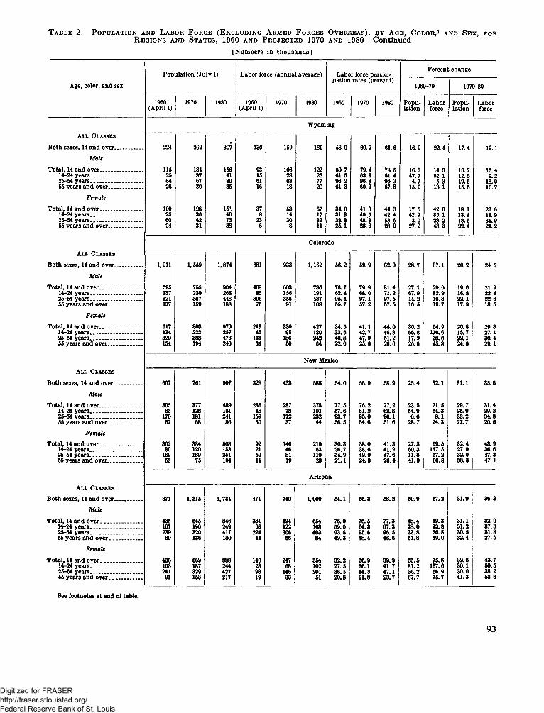
T a b l e 2 . P o p u l a t io n a n d L a b o r F o r c e (E x c l u d in g A r m e d F o r c e s O v e r s e a s ) , b y A g e , C o lo r , 1 a n d S e x , f o r R e g io n s a n d S t a t e s , 1960 a n d P r o je c t e d 1970 a n d 1980—Continued
[Numbers in thousands]
Age, color, and sexPopulation (July 1) Labor force (annual average) Labor force participation rates (percent)
Percent1960-70
tchange1970-80
1960(April 1) 1970 1980 1960(April 1) 1970 1980 1960 1970 1980 Population Laborforce Population LaborforceWyoming
A l l C l a s s e s
Both sexes, 14 and over.................. 224 262 307 130 159 189 58.0 60.7 61.6 16.9 22.4 17.4 19.1M ale
Total, 14 and over........................... 115 134 156 93 106 122 80.7 79.4 78.5 16.3 14.3 16.7 15.414-24 years................................. 25 37 41 15 23 25 61.5 63.3 61.4 47.7 52.1 12.5 9.225-54 years........ ........................ 64 67 80 61 63 77 96.2 96.8 96.3 4.7 5.3 19.5 18.955 years and over...................... 26 30 35 16 18 20 61.3 60.3 57.8 15.0 13.1 15.5 10.7F em ale
Total, 14 and over.......................... 109 128 151 37 53 67 34.0 41.3 44.3 17.5 42.6 18.1 26.614-24 years................................. 25 36 40 8 14 17 31.3 40.5 42.4 42.9 85.1 13.4 18.925-54 years................................. 60 62 73 23 30 39 38.8 48.3 53.6 3.0 28.2 18.6 31.955 years and over..................... 24 31 38 6 8 11 25.1 28.3 28.0 27.2 43.3 22.4 21.2
ColoradoA l l C l a s s e s
Both sexes, 14 and over.................. 1,211 1,559 1,874 681 933 1,162 56.2 59.9 62.0 28.7 37.1 20.2 24.5M ale
Total, 14 and over........................... 595 755 904 468 603 736 78.7 79.9 81.4 27.1 29.0 19.6 21.914-24 years................................ 137 230 268 85 156 191 62.4 68.0 71.2 67.9 82.9 16.8 22.425-54 years................................. 321 367 448 306 356 437 95.4 97.1 97.5 14.2 16.3 22.1 22.655 years and over..................... 137 159 188 76 91 108 55.7 57.2 57.5 16.5 19.7 17.9 18.5F em ale
Total, 14 and over........................... 617 803 970 213 330 427 34.5 41.1 44.0 30.2 54.9 20.8 29.314-24 years............................... . 134 222 257 45 95 120 33.6 42.7 46.8 65.8 110.6 15.7 27.125-54 years................................. 329 388 473 134 186 242 40.8 47.9 51.2 17.9 38.6 22.1 30.455 years and over...................... 154 194 240 34 50 64 22.0 25.6 26.6 25.5 45.8 24.0 29.1New Mexico
A l l C l a s s e s
Both sexes, 14 and over.................. 607 761 997 328 433 588 54.0 56.9 58.9 25.4 32.1 31.1 35.6M ale
Total, 14 and over........................... 305 377 489 236 287 378 77.5 76.2 77.2 23.5 21.5 29.7 31.414-24 years................................. 83 128 161 48 78 101 57.6 61.2 62.8 54.9 64.3 25.9 29.225-54 years................................. 170 181 241 159 172 232 93.7 95.0 96.1 6.6 8.1 33.2 34.855 years and over..................... 52 68 86 30 37 44 56.5 54.6 51.6 28.7 24.3 27.7 20.6F em ale
Total, 14 and over.......................... 302 384 508 92 146 210 30.3 38.0 41.3 27.3 59.5 32.4 43.914-24 years................................. 80 120 153 21 46 63 26.7 38.6 41.2 50.3 117.5 27.9 36.625-54 years............. ........... ...... 169 189 251 59 81 119 34.9 42.9 47.6 11.8 37.2 32.9 47.355 years and over..................... 53 75 104 11 19 28 21.1 24.8 26.4 41.9 66.8 38.3 47.1Arizona
A l l C l a s s e s
Both sexes, 14 and over.................. 871 1,315 1,734 471 740 1,009 54.1 56.3 58.2 50.9 57.2 31.9 36.3M ale
Total, 14 and over.......................... 435 645 846 331 494 654 76.0 76.5 77.3 48.4 49.3 31.1 32.614-24 years............... ................ 107 190 249 63 122 168 59.0 64.3 67.3 78.0 93.8 31.2 37.325-54 years................................. 239 320 417 224 306 403 93.5 95.6 96.5 33.8 36.8 30.5 31.855 years and over..................... 89 136 180 44 66 84 49.3 48.4 46.6 51.8 49.0 32.4 27.5F em ale
Total, 14 and over................... ....... 436 669 888 140 247 354 32.2 36.9 39.9 53.5 75.8 32.6 43.714-24 years................................ 103 187 244 28 68 102 27.5 36.1 41.7 81.2 137.6 30.1 50.525-54 years........................... 1__ 241 329 427 93 146 201 38.5 44.3 47.1 36.2 56.9 30.0 38.255 years and over..................... 91 153 217 19 33 51 20.8 21.8 23.7 67.7 75.7 41.3 53.6
See footnotes at end of table.
93
Digitized for FRASER http://fraser.stlouisfed.org/ Federal Reserve Bank of St. Louis
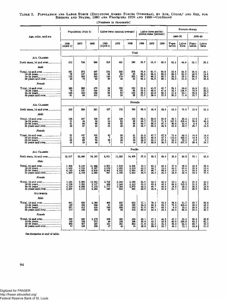
T a b l e 2 . P o p u l a t io n a n d L a b o r F o r c e (E x c l u d in g A r m e d F o r c e s O v e r s e a s ), b y A g e , C o l o r ,1 a n d S e ;x , f o r R e g io n s a n d S t a t e s , 1960 a n d P r o je c t e d 1970 a n d 1980—Continued
[Numbers in thousands]
Population (July 1) Labor force (annual average) Labor force partici Percent changeAge, color, and sex pation rates (percent) 1960-70 1970-80
1960(April 1) 1970 1980 1960(April 1) 1970 1980 1960 1970 1980 Population Laborforce Population LaborforceUtah
A l l C l a s s e s
Both sexes, 14 and over.................. 572 756 946 319 461 596 55.7 61.0 63.0 32.2 44.8 25.1 29.2Male
Total, 14 and over.......................... 281 373 467 224 302 378 79.8 81.0 80.8 32.4 34.5 25.4 25.114-24 years................................. 74 117 140 44 80 95 59.4 68.4 68.3 59.0 82.9 19.6 19.425-54 years................................. 152 185 242 145 179 232 9517 96.2 95.7 22.5 23.2 30.4 29.855 years and over..................... 56 70 85 36 43 50 63.2 61.8 59.1 24.0 21.3 21.7 16.3Female
Total, 14 and over.......................... 290 383 479 94 159 219 32.4 41.6 45.7 32.1 69.4 24.9 37.114-24 years................................ 79 121 144 26 53 68 33.0 43.8 47.4 54.1 104.6 18.8 28.625-54 years................................ 150 182 234 54 82 118 36.2 45.3 50.3 21.4 52.1 28.6 42.755 years and over..................... 61 80 101 14 24 33 22.7 29.9 32.5 30.2 71.4 25.7 36.5Nevada
A l l C l a s s e s
Both sexes, 14 and over.................. 202 334 381 127 218 243 63.0 65.4 63.8 65.5 71.6 13.9 11.2Male
Total, 14 and over......................... - 105 167 189 87 139 152 83.1 83.0 80.6 59.1 58.9 12.9 9.714-24 years............................... 21 45 54 14 32 38 66.7 72.8 71.2 107.5 126.4 20.9 18.225-54 years............................... - 61 86 90 58 83 88 95.7 96.8 97.0 40.6 42.4 5.4 5.655 years and over...................... 23 37 45 15 23 26 64.7 63.2 58.9 62.8 59.0 20.7 12.3Female
Total, 14 and over....................... 97 167 192 40 80 91 41.3 47.7 47.3 72.4 99.2 14.9 14.014-24 years........ ........ .......... . 21 43 50 7 20 23 33.8 45.8 47.1 110.6 186.0 14.4 17.625-54 years............... ................. 58 89 94 28 49 54 48.3 55.2 57.4 53.8 76.0 5.5 9.755 years and over...................... 19 35 48 5 11 14 27.9 30.8 28.0 87.8 107.3 39.4 26.7Pacific
A l l C l a s s e s
Both sexes, 14 and over.................. 15,017 19,490 24,182 8,611 11,565 14,495 57.3 59.3 59.9 29.8 34.3 24.1 25.3Male
Total, 14 and over.......................... 7,466 9,510 11,688 5,907 7,616 9,401 79.1 80.1 80.4 27.4 28.9 22.9 23.414-24 years________________ 1,633 2,718 3,287 1,019 1,895 2,319 62.5 69.7 70.6 66.5 85.8 20.9 22.425-54 years............. ................. 4,142 4,680 5,818 3,941 4,525 5,630 95.1 96.7 96.8 13.0 14.8 24.3 24.455 years and over..................... 1,692 2,113 2,583 947 1,196 1,452 56.0 56.6 56.2 24.9 26.4 22.3 21.4Female
Total, 14 and over........................... 7,551 9,980 12,493 2,703 3,949 5,094 35.8 39.6 40.8 32.2 46.1 25.2 29.014-24 years________________ 1,529 2,582 3,137 488 1,043 1,415 2,873 32.0 40.4 45.1 68.9 113.5 21.5 35.725-54 years................................ 4,116 4,888 6,123 1,777 2,284 43.2 46.7 46.9 18.8 28.5 25.3 25.855 years and over...................... 1,901 2,510 3,234 438 622 805 23.0 24.8 24.9 31.7 42.1 28.8 29.4N o n w h i t e
MaleTotal, 14 and over................ .......... 641 830 1,086 495 652 852 77.1 78.5 78.5 29.5 31.7 30.7 30.814-24 years................................. 148 262 368 81 166 238 54.4 63.4 64.7 76.5 105.8 40.5 43.525-54 years________ _______ 381 415 525 346 393 502 91.0 94.7 95.7 9.0 13.5 26.5 27.8
55 years and over...................... 112 153 193 68 93 112 60.3 60.5 58.1 36.6 36.9 25.6 20.7Female
Total, 14 and over.......................... 598 850 1,173 258 401 543 43.1 47.1 46.3 42.2 55.4 38.0 35.614-24 years............................. . 143 258 370 44 103 168 30.4 40.1 45.3 80.0 136.8 43.2 62.125-54 years............................. . 362 457 597 187 251 302 51.8 55.0 50.5 26.3 34.1 30.7 20.055 years and over...................... 92 135 206 27 46 74 28.8 33.9 35.7 46.0 72.1 52.8 61.0
See footnotes at end of table.
94
Digitized for FRASER http://fraser.stlouisfed.org/ Federal Reserve Bank of St. Louis
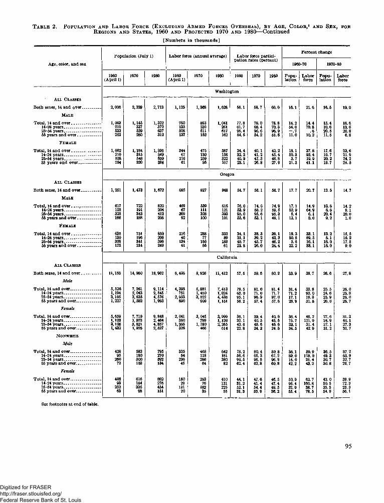
Table 2. Population and Labor Force (Excluding Armed Forces Overseas), by Age, Color,1 and Sex, fo r Regions and States, 1960 and Projected 1970 and 1980— Continued[Numbers in thousands]
Age, color, and sexPopulation (July 1) Labor force (annual average) Labor force participation rates (percent)
Percent1960-70
change1970-80
1960(April 1) 1970 1980 1960(April 1) 1970 1980 1960 1970 1980 Population Laborforce Population LaborforceWashington
All ClassesBoth sexes, 14 and over................ 2,006 2,329 2,713 1,125 1,368 1,628 56.1 58.7 60.0 16.1 21.6 16.5 19.0
MaleTotal, 14 and over.......................... 1,003 1,145 1,322 780 893 1,041 77.8 78.0 78.8 14.2 14.4 15.4 16.614-24 years................................. 219 337 372 135 230 261 61.7 68.4 70.3 54.0 70.8 10.6 13.625-54 years................................ 533 529 637 508 511 617 95.4 96.6 96.9 - . 7 .6 20.5 20.855 years and over..................... 252 280 312 137 152 162 54.5 54.2 51.8 11.0 10.2 11.5 6.8
FemaleTotal, 14 and over.......................... 1,002 1,184 1,391 344 475 587 34.4 40.1 42.2 18.1 37.8 17.6 23.614-24 years................................. 210 315 349 67 130 158 32.2 41.2 45.4 50.3 92.4 10.7 21.925-54 years............... ................. 528 548 659 216 259 322 40.9 47.3 48.8 3.7 19.9 20.2 24.255 years and over.................... 264 320 384 61 86 107 23.1 26.8 27.9 21.3 41.1 19.7 24.5
OregonAll Classes
Both sexes, 14 and over.................. 1,251 1,473 1,672 685 827 948 54.7 56.1 56.7 17.7 20.7 13.5 14.7Male
Total, 14 and over.......................... 617 722 822 469 539 615 76.0 74.6 74.9 17.1 14.9 13.8 14.214-24 years................................ 125 191 204 67 111 121 53.9 58.2 59.5 52.9 64.9 6.6 9.125-54 years.................... ............ 325 343 412 309 328 393 95.0 95.6 95.3 5.4 6.1 20.4 20.055 years and over..................... 166 188 205 92 100 101 55.6 53.1 49.1 13.1 8.0 9.2 1.0Female
Total, 14 and over____ ________ 635 751 850 216 288 333 34.1 38.3 39.1 18.3 33.1 13.2 15.514-24 years............... - ............... 130 196 206 40 77 89 31.1 39.2 43.3 50.5 89.5 5.1 16.225-54 years................................ 329 341 396 134 156 183 40.7 45.7 46.2 3.6 16.1 16.0 17.555 years and over..................... 175 214 249 41 56 61 23.8 26.0 24.4 22.2 33.1 16.0 9.0California
All ClassesBoth sexes, 14 and over................. 11,185 14,980 18,962 6,436 8,926 11, 412 57.5 59.6 60.2 33.9 38.7 26.6 27.8
MaleTotal, 14 and over...____ ______ 5,526 7,261 9,114 4,395 5,881 7,413 79.5 81.0 81.4 31.4 33.8 25.5 26.014-24 years...... ........ ................ 1,194 2,043 2,545 751 1,450 1,824 63.0 71.0 71.7 71.2 93.0 24.6 25.825-54 years...................... ......... 3,105 3,635 4,576 2,953 3,522 4,438 95.1 96.9 97.0 17.1 19.3 25.9 26.055 years and over..................... 1,227 1,582 1,993 690 909 1,151 56.2 57.4 57.8 28.9 31.8 26.0 26.7
FemaleTotal, 14 and over.......................... 5,659 7,719 9,848 2,041 3,045 3,999 36.1 39.4 40.6 36.4 49.2 27.6 31.314-24 years............. ................ l, 123 1,973 2,464 360 799 1,120 32.1 40.5 45.5 75.7 121.9 24.9 40.125-54 years_______ ________ 3,105 3,821 4,857 1,355 1,780 2,265 43.6 46.6 46.6 23.1 31.4 27.1 27.355 years and over.............. ...... 1,432 1,926 2,527 326 466 614 22.8 24.2 24.3 34.5 42.9 31.2 31.7
N onwhiteMale
Total, 14 and over........................... 428 583 795 335 468 642 78.2 80.4 80.8 36.1 39.9 36.5 37.214-24 years............. ................ 95 180 270 54 118 181 56.6 65.3 67.2 89.0 118.0 49.3 53.925-54 years_________ _______ 260 300 392 236 286 380 90.5 95.5 96.9 15.0 21.4 30.7 32.755 years and over..................... 72 103 134 45 64 82 62.4 62.8 60.8 42.2 43.2 30.8 26.7Female
Total, 14 and over.......................... 408 616 882 180 293 410 44.1 47.6 46.5 50.9 62.7 43.0 39.914-24 years................................. 93 184 276 29 76 131 31.2 41.4 47.4 96.4 160.8 50.5 72.325-54 years...... ...................... 252 335 454 131 182 225 52.1 54.4 49.5 32.9 38.7 35.5 23.355 years and over..................... 63 98 151 20 35 55 31.3 35.9 36.2 55.4 78.5 54.9 56.1
See footnotes at end of table.
95
Digitized for FRASER http://fraser.stlouisfed.org/ Federal Reserve Bank of St. Louis
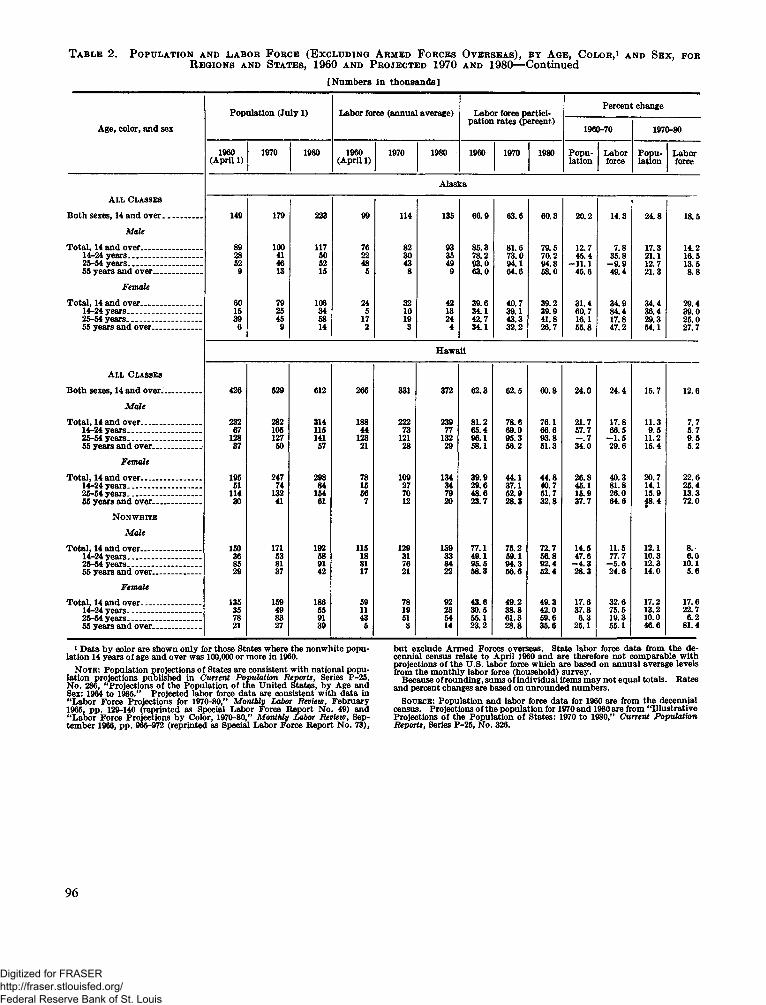
Table 2. Population and .labor Force (Excluding Armed Forces Overseas), by Age, Color,1 and Sex, for Regions and States, 1960 and Projected 1970 and 1980—Continued[Numbers in thousands]
P o p u la t io n ( J u l y 1 ) L a b o r fo rc e ( a n n u a l a v e r a g e ) L a b o r fo rc e p a r t ic i P e r c e n t c h a n g e
A g e , c o lo r , a n d s e xp a t io n r a t e s ( p e r c e n t)
19 6 0 -7 0 19 7 0 -8 0
19 6 0( A p r i l 1 )
19 7 0 19 8 0 19 6 0( A p r i l 1 )
19 7 0 19 8 0 196 0 19 7 0 1980 P o p u la t io n
L a b o rfo rc e
P o p u la t io n
L a b o rfo rce
A l a s k a
All ClassesB o t h s e x e s , 1 4 a n d o v e r ........................ 14 9 17 9 2 2 3 99 1 1 4 1 3 5 6 6 .9 6 3 .6 6 0 .3 2 0 .2 1 4 . 3 2 4 .8 1 8 .5
M aleT o t a l , 1 4 a n d o v e r ..................................... 89 10 0 1 1 7 76 82 93 8 5 .3 8 1 .6 7 9 .5 1 2 . 7 7 .8 1 7 . 3 1 4 .2
14 - 2 4 y e a r s ............................................. 28 4 1 50 22 30 3 5 7 8 .2 7 3 .0 7 0 .2 4 5 .4 3 5 .8 2 1 . 1 1 6 .52 5 -5 4 y e a r s ............................................ 52 46 52 48 43 49 9 3 .0 9 4 . 1 9 4 .8 - 1 1 . 1 - 9 . 9 1 2 .7 1 3 . 55 5 y e a r s a n d o v e r .............................. 9 1 3 1 5 5 8 9 6 3 .0 6 4 .6 5 8 .0 4 5 .6 4 9 .4 2 1 . 3 8 .8
FemaleT o t a l , 1 4 a n d o v e r ..................................... 60 79 10 6 24 3 2 42 3 9 .6 4 0 .7 3 9 .2 3 1 . 4 3 4 .9 3 4 .4 2 9 .4
14 -2 4 y e a r s ........... ................................. 1 5 25 34 5 1 0 1 3 3 4 . 1 3 9 . 1 3 9 .9 6 0 .7 8 4 .4 3 6 .4 3 9 .02 5 -5 4 y e a r s ............................................. 39 45 58 1 7 19 24 4 2 .7 4 3 .3 4 1 .8 1 6 . 1 1 7 .8 2 9 .3 2 5 .055 y e a r s a n d o v e r .............................. 6 9 14 2 3 4 3 4 . 1 3 2 .2 2 6 .7 5 5 .8 4 7 .2 5 4 . 1 2 7 .7
H a w a i i
All ClassesB o t h se x e s , 1 4 a n d o v e r . ...................... 426 529 6 12 266 3 3 1 37 2 6 2 .3 6 2 .5 6 0 .8 2 4 .0 2 4 .4 1 5 . 7 1 2 .6
M aleT o t a l , 1 4 a n d o v e r .................................... 2 32 282 3 1 4 18 8 222 2 39 8 1 . 2 7 8 .6 7 6 . 1 2 1 . 7 1 7 . 8 1 1 . 3 7 .7
1 4 - 2 4 y e a r s ............................................ 67 10 5 1 1 5 44 7 3 77 6 5 .4 6 9 .0 6 6 .6 5 7 .7 6 6 .5 9 .5 5 .72 5 -5 4 y e a r s ............................................ 12 8 12 7 1 4 1 1 2 3 1 2 1 1 3 2 9 6 .1 9 5 .3 9 3 .8 - . 7 - 1 . 5 1 1 . 2 9 .55 5 y e a r s a n d o v e r ............................. 3 7 50 57 2 1 28 29 5 8 . 1 5 6 .2 5 1 . 3 3 4 .0 2 9 .6 1 5 . 4 5 .2
FemaleT o t a l , 1 4 a n d o v e r .................................... 19 5 247 298 78 10 9 1 3 4 3 9 .9 4 4 . 1 4 4 .8 2 6 .8 4 0 .3 2 0 .7 2 2 .6
14 - 2 4 y e a r s ............................................. 5 1 74 84 1 5 2 7 34 2 9 .6 3 7 . 1 4 0 .7 4 5 . 1 8 1 .8 1 4 . 1 2 5 .42 5 - 5 4 y e a r s ............................................ 1 1 4 1 3 2 15 4 56 70 79 4 8 .6 5 2 .9 5 1 . 7 1 5 . 9 2 6 .0 1 5 . 9 1 3 . 35 5 y e a r s a n d o v e r ............................. 30 4 1 6 1 7 1 2 20 2 3 .7 2 8 .3 3 2 .8 3 7 .7 6 4 .6 4 8 .4• 7 2 .0
N onwhiteM ale
T o t a l , 1 4 a n d o v e r .................................... 15 0 1 7 1 19 2 1 1 5 12 9 13 9 7 7 . 1 7 5 .2 7 2 .7 1 4 . 5 1 1 . 5 1 2 . 1 8.14 - 2 4 y e a r s ............................................ 36 5 3 58 1 8 3 1 3 3 4 9 . 1 5 9 . 1 5 6 .8 4 7 .6 7 7 .7 1 0 . 3 6 .02 5 - 5 4 y e a r s ............................................ 85 8 1 9 1 8 1 76 84 9 5 .5 9 4 .3 9 2 .4 - 4 . 3 - 5 . 6 1 2 . 3 1 0 . 15 5 y e a r s a n d o v e r ............................. 29 3 7 42 1 7 2 1 2 2 5 8 .3 5 6 .6 5 2 .4 2 8 .3 2 4 .6 1 4 .0 5 .6
FemaleT o t a l , 1 4 a n d o v e r .................................... 1 3 5 15 9 18 6 59 78 92 4 3 .6 4 9 .2 4 9 .3 1 7 .6 3 2 .6 1 7 . 2 1 7 . 6
14 - 2 4 y e a r s ............. - ............................ 3 5 49 55 1 1 19 2 3 3 0 .5 3 8 .8 4 2 .0 3 7 .8 7 5 .5 1 3 . 2 2 2 .72 5 -5 4 y e a r s . .............- .......................... 78 83 9 1 43 5 1 54 5 5 . 1 6 1 . 3 5 9 .6 6 .3 1 9 . 3 1 0 .0 6 .25 5 y e a r s a n d o v e r . . ................. .. 2 1 27 39 5 8 1 4 2 3 .2 2 8 .8 3 5 .6 2 5 . 1 5 5 . 1 4 6 .6 8 1 . 4
1 D a t a b y c o lo r a r e s h o w n o n ly fo r th o se S t a t e s w h e r e th e n o n w h it e p o p u la t io n 1 4 y e a r s o f a g e a n d o v e r w a s 100 ,000 o r m o r e in 1960.
N ote: P o p u la t io n p r o je c t io n s o f S t a t e s a r e c o n s is te n t w i t h n a t io n a l p o p u la t io n p r o je c t io n s p u b lis h e d in Current Population Reports, S e r ie s P - 2 5 , N o . 286, “ P r o je c t io n s o f th e P o p u la t io n o f th e U n it e d S t a t e s , b y A g e a n d S e x : 19 6 4 to 19 8 5 .” P r o je c t e d la b o r fo rce d a t a a r e c o n s is te n t w i t h d a t a in “ L a b o r F o r c e P r o je c t io n s fo r 19 7 0 -8 0 ,” M onthly Labor Review, F e b r u a r y 19 6 5 , p p . 12 9 - 14 0 ( r e p r in t e d a s S p e c ia l L a b o r F o r c e R e p o r t N o . 49) a n d “ L a b o r F o r c e P r o je c t io n s b y C o lo r , 19 7 0 -8 0 ,” M onthly Labor Review, S e p t e m b e r 19 6 6 , p p . 9 6 5-9 72 ( r e p r in t e d a s S p e c ia l L a b o r F o r c e R e p o r t N o . 7 3 ) ,
b u t e x c lu d e A r m e d F o r c e s o v e r s e a s . S t a t e la b o r fo rc e d a t a fr o m th e d e c e n n ia l c e n s u s r e la t e to A p r i l 19 6 0 a n d a r e th e re fo r e n o t c o m p a r a b le w i t h p r o je c t io n s o f th e U .S . la b o r fo rce w h ic h a r e b a s e d o n a n n u a l a v e r a g e le v e ls f r o m th e m o n t h ly la b o r fo rc e (h o u se h o ld ) s u r v e y .
B e c a u s e o f r o u n d in g , s u m s o f in d iv id u a l i te m s m a y n o t e q u a l to t a ls . R a t e s a n d p e r c e n t c h a n g e s a r e b a s e d o n u n r o u n d e d n u m b e r s .
Source: P o p u la t io n a n d la b o r fo rc e d a t a fo r 196 0 a r e fr o m th e d e c e n n ia l c e n s u s . P r o je c t io n s o f th e p o p u la t io n fo r 19 7 0 a n d 19 8 0 a r e fr o m “ I l lu s t r a t i v e P r o je c t io n s o f th e P o p u la t io n o f S t a t e s : 19 7 0 to 19 8 0 ,” Current Population R eports , S e r ie s P - 2 5 , N o . 326 .
96
Digitized for FRASER http://fraser.stlouisfed.org/ Federal Reserve Bank of St. Louis
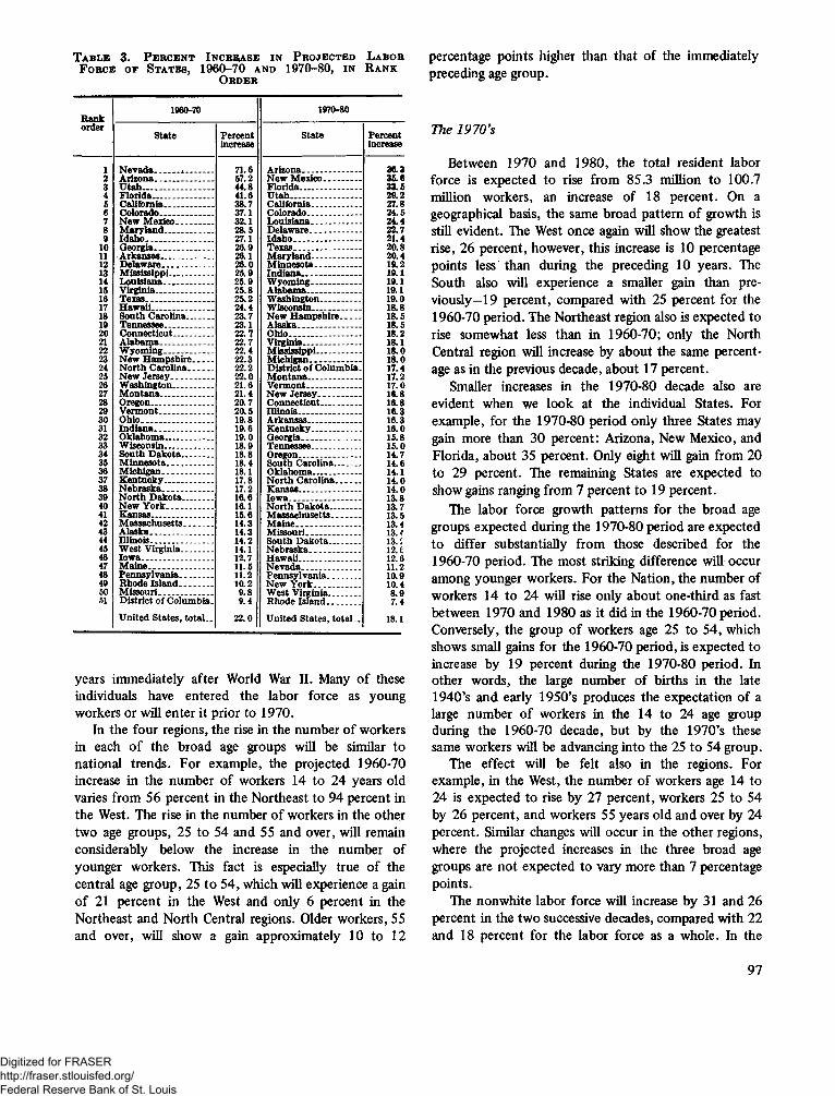
Table 3. Percent Increase in Projected Labor percentage points higher than that of the immediatelyForce of States, 1960-70 and 1970-80, in Rank preceding age group.
R a n k19 6 0 -70 19 7 0 -8 0
o r d e rS t a t e P e r c e n t S t a t e P e r c e n t
in c re a se in c re a se
1 N e v a d a . . . . x _______ 7 1 .6 A r i z o n a ____________ ___ 3 6 .32 A r i z o n a ........... ..................... 5 7 .2 N e w M e x i c o . . ............... 3 5 .63 U t a h ....................................... 4 4 .8 F l o r i d a .................................. 3 3 . 54 F l o r i d a .................................. 4 1 .6 U t a h ........................... ........... 2 9 .25 C a l i f o r n ia ............... ........... 3 8 .7 C a l i f o r n ia _____ ________ 2 7 .86 C o lo r a d o . _____ 3 7 . 1 C o lo r a d o _______________ 2 4 .57 N e w M e x i c o _________ 3 2 . 1 L o u i s i a n a ______________ 2 4 .48 M a r y l a n d ...................... 2 8 .5 D e la w a r e ............................. 2 2 .79 I d a h o ........... .......................... 2 7 . 1 I d a h o . .................... .............. 2 1 . 4
1 0 G e o r g ia ................................. 2 6 .9 T e x a s ..................................... 2 0 .81 1 - A r k a n s a s . . _ ___ 2 6 . 1 M a r y l a n d ........................... 2 0 .412 D e l a w a r e . .......................... 2 6 .0 M in n e s o t a ........... .............. 1 9 . 21 3 M is s i s s ip p i ........................ 2 5 .0 I n d i a n a . . ............................ 1 9 . 11 4 L o u i s i a n a ........ ................... 2 5 .9 W y o m in g _____________ 1 9 . 11 5 V i r g i n i a ...................... . 2 5 .8 A l a b a m a _______________ 1 9 . 116 T e n s ................................... 2 5 .2 W a s h in g t o n ___________ 1 9 .01 7 H a w a i i ................. ................ 2 4 .4 W is c o n s in ........................... 1 8 .818 S o u t h C a r o l i n a .......... 2 3 .7 N e w H a m p s h i r e _____ 1 8 . 519 T e n n e s s e e . . ...................... 2 3 . 1 A l a s k a ................................... 1 8 . 520 C o n n e c t ic u t ...................... 2 2 .7 O h io ........................................ 1 8 . 22 1 A la b a m a .............................. 2 2 .7 V i r g in ia ________________ 1 8 . 122 W y o m i n g ........................... 2 2 .4 M is s i s s ip p i ..............._ ....... 1 8 . 02 3 N e w H a m p s h ir e ........... 2 2 .3 M ic h i g a n ________ ______ 1 8 .024 N o r t h C a r o l i n a .............. 2 2 .2 D i s t r ic t o f C o lu m b i a . 1 7 . 42 5 N e w J e r s e y ....................... 2 2 .0 M o n t a n a ...................... ....... 1 7 . 226 W a s h in g t o n ___________ 2 1 .6 V e r m o n t _______________ 1 7 . 02 7 M o n t a n a ............................. 2 1 . 4 N e w J e r s e y . ..................... 1 6 .828 O re g o n .................................. 2 0 .7 C o n n e c t ic u t .......... ............ 1 6 .829 V e r m o n t .............................. 2 0 .5 I l l i n o i s .................... .............. 1 6 . 33 0 O h io ........... ............................ 1 9 .8 A r k a n s a s ...................... ....... 1 6 . 33 1 I n d i a n a . .............................. 1 9 .6 K e n t u c k y . . ________ 1 6 .03 2 O k la h o m a .............. ............ 1 9 .0 G e o r g ia . . __________ 1 5 . 83 3 W is c o n s in .......... ................ 1 8 .9 T e n n e s s e e _______ _____ 1 5 . 034 S o u t h D a k o t a _________ 1 8 .8 O re g o n _________________ 1 4 .73 5 M in n e s o t a .......................... 1 8 .4 S o u t h C a r o l i n a ............... 1 4 .636 M ic h i g a n ............................ 1 8 . 1 O k la h o m a _____________ 1 4 . 13 7 K e n t u c k y ........................... 1 7 .8 N o r t h C a r o l i n a .............. 1 4 .038 N e b r a s k a ............................ 1 7 . 2 K a n s a s . . . . ................. 1 4 . 039 N o r t h D a k o t a ................. 1 6 .6 I o w a ............. ......... ................ 1 3 . 840 N e w Y o r k .......................... 1 6 . 1 N o r t h D a k o t a . ............ 1 3 . 74 1 K a n s a s . . . 1 5 .6 M a s s a c h u s e t t s 1 3 . 542 M a s s a c h u s e t t s ________ 1 4 . 3 M a i n e __________________ 1 3 .443 A l a s k a ......................... ......... 1 4 . 3 M is s o u r i 1 3 .444 I l l i n o i s ........................... .. 1 4 . 2 S o u t h D a k o t a ............. 1 3 . 145 W e s t V i r g i n i a .................. 1 4 . 1 N e b r a s k a . ..................... 1 2 . e46 I o w a .................... .................. 1 2 . 7 H a w a i i . 1 2 .647 M a i n e ................................... 1 1 . 5 N e v a d a . . 1 1 . 248 P e n n s y l v a n i a .................. 1 1 . 2 P e n n s y lv a n i a 1 0 .949 R h o d e I s l a n d ................... 1 0 . 2 N e w Y o r k . . 1 0 .450 M is s o u r i .............................. 9 .8 W e s t V i r g i n i a . 8 .95 1 D is t r ic t o f C o lu m b ia . 9 .4 R h o d e I s l a n d _________ 7 .4
U n it e d S t a t e s , t o t a l . . 2 2 .0 U n it e d S t a t e s , t o t a l . . 1 8 . 1
years immediately after World War II. Many of these individuals have entered the labor force as young workers or will enter it prior to 1970.
In the four regions, the rise in the number of workers in each of the broad age groups will be similar to national trends. For example, the projected 1960-70 increase in the number of workers 14 to 24 years old varies from 56 percent in the Northeast to 94 percent in the West. The rise in the number of workers in the other two age groups, 25 to 54 and 55 and over, will remain considerably below the increase in the number of younger workers. This fact is especially true of the central age group, 25 to 54, which will experience a gain of 21 percent in the West and only 6 percent in the Northeast and North Central regions. Older workers, 55 and over, will show a gain approximately 10 to 12
The 19 70 fsBetween 1970 and 1980, the total resident labor
force is expected to rise from 85.3 million to 100.7 million workers, an increase of 18 percent. On a geographical basis, the same broad pattern of growth is still evident. The West once again will show the greatest rise, 26 percent, however, this increase is 10 percentage points less than during the preceding 10 years. The South also will experience a smaller gain than previously—19 percent, compared with 25 percent for the 1960-70 period. The Northeast region also is expected to rise somewhat less than in 1960-70; only the North Central region will increase by about the same percentage as in the previous decade, about 17 percent.
Smaller increases in the 1970-80 decade also are evident when we look at the individual States. For example, for the 1970-80 period only three States may gain more than 30 percent: Arizona, New Mexico, and Florida, about 35 percent. Only eight will gain from 20 to 29 percent. The remaining States are expected to show gains ranging from 7 percent to 19 percent.
The labor force growth patterns for the broad age groups expected during the 1970-80 period are expected to differ substantially from those described for the 1960-70 period. The most striking difference will occur among younger workers. For the Nation, the number of workers 14 to 24 will rise only about one-third as fast between 1970 and 1980 as it did in the 1960-70 period. Conversely, the group of workers age 25 to 54, which shows small gains for the 1960-70 period, is expected to increase by 19 percent during the 1970-80 period. In other words, the large number of births in the late 1940’s and early 1950’s produces the expectation of a large number of workers in the 14 to 24 age group during the 1960-70 decade, but by the 1970’s these same workers will be advancing into the 25 to 54 group.
The effect will be felt also in the regions. For example, in the West, the number of workers age 14 to 24 is expected to rise by 27 percent, workers 25 to 54 by 26 percent, and workers 55 years old and over by 24 percent. Similar changes will occur in the other regions, where the projected increases in the three broad age groups are not expected to vary more than 7 percentage points.
The non white labor force will increase by 31 and 26 percent in the two successive decades, compared with 22 and 18 percent for the labor force as a whole. In the
97
Digitized for FRASER http://fraser.stlouisfed.org/ Federal Reserve Bank of St. Louis
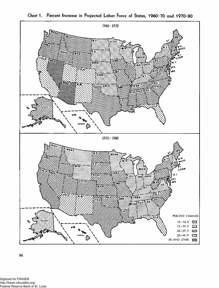
Chart 1. Percent Increase in Projected Labor Force of States, 1960-70 and 1970-801960- 1970
1970- 1980
PERCENT CHANGE10-14.9 E S 15-19.9 EU 20-29.9 30-49.9 E 3
50 AND OVER H
98
Digitized for FRASER http://fraser.stlouisfed.org/ Federal Reserve Bank of St. Louis
South and West, the non white labor force will increase only slightly faster than the total for the region. In the Northeast and North Central regions, the nonwhite labor force will grow at about twice the rate for the whole labor force. These data have significant implications for education and employment policies in all of these regions.R elia b ility
Before describing the methods used in making these projections some discussion of the limitations affecting the reliability of these projections is necessary. First, the most important element in the size of the projected labor force of each State is the projection of the population of working age. In projecting the population for the next 10 or 15 years, the most critical variable is the magnitude and composition of net interstate migration. Our selection of the Series II migration assumption cannot be supported by specific evidence; it reflects our judgment that interstate migration is essentially purposive movement which occurs to a considerable degree in response to differential economic opportunities. Limited evidence exists that these differentials tend to decline over time, partly as a result of the population movements they originally inspire.6 We therefore selected the series which assumes a very gradual decline in the net interstate migration in preference to the series which assumed a constant rate equal to that observed during 1955-60. Alternative assumptions in regard to the volume and direction of interstate migration in the future would result in a considerably different set of population projections, and, therefore, would yield different labor force projections as well. For example, the number of workers in the State of California, where net immigration is substantial, would be 135,000 (1.0 percent) greater than our projection of 13.4 million if the “high migration” assumption had been employed. Conversely, assuming no net migration would yield a labor force 302,000 (2.2 percent) less. In comparison, the high migration assumption for the State of Maine would produce a 1970 labor force only 5,000 (0.7 percent) less than our projection of 669,000, and the assumption of no net migration would yield a labor force 11,000 (1.6 percent) greater. For most of the States, the effect of the alternative migration assumptions would fall within the range indicated in the above examples.
6 Lowell D. Ashby, “The Geographical Redistribution of Employment: An Examination of the Elements of Change,” Survey o f Current Business, October 1944, pp. 13-20.
Second, in projecting the labor force participation rates (percent of population in the labor force for specific age groups of men and women), the procedure that was applied to past labor force participation rates was the same for each State. The chief merits of this approach are its simplicity and objectivity. The chief limitation is its failure to take explicit account of past economic or social circumstances of a State which are not expected to continue, or possible special future circumstances which could affect the labor force participation rates for some States. For this reason, these projections should be regarded only as a very approximate indication of future developments. They should not be regarded as a substitute for more detailed projections which might be prepared for any particular State on the basis of a careful analysis of its peculiar circumstances and developmental policies.7
In view of these limitations, we would appreciate comments or suggestions from users of these data in regard to their usefulness and improvements. We also would welcome any examples of projections that may have been developed by users for local areas, together with information as to techniques employed in their development.
The procedure used in projecting the labor force has four essential steps. First, for each age-sex-color group, the labor force participation rate for 1940, 1950, and 1960 for each State was expressed as a ratio of the corresponding national labor force participation rate. Next, these ratios were extrapolated to 1970 and 1980 by extending the trend shown by the three past observations. Then the extrapolated ratios were applied to independently projected national labor force participation rates for 1970 and 1980. Finally, the projected labor force participation rates were applied to the projected population for each age-sex-color cell for the States. The effect of this procedure is to take specific account of differences among States in the rates for each age-sex-color group, and the trend in these differences over the 1940-60 period, in projecting the relationship of the rates for each State to the national average.M eth o d
As was stated earlier, the State labor force projections were prepared by a procedure consisting of four basic
7 According to the results of a recent mail survey by the Census Bureau, at least 30 State agencies carry out population projections for their own Use. In addition, in nearly every State, one or more universities or private organizations engage in population projections as a part of their research or planning activities. See the Bureau of the Census, “Inventory of State and Local Agencies Preparing Population Estimates-Survey of 1965,” Current Population R eports, Series P-25, No. 328.
99
Digitized for FRASER http://fraser.stlouisfed.org/ Federal Reserve Bank of St. Louis
steps. First approximations and successive adjustments were obtained by using a special program written in FORTRAN language for the IBM 7074 computer. The basic inputs were: (1) State labor force participation rates, by age, sex, and color, for 1940,1950, and I960;8(2) national labor force participation rates, by age, sex, and color, for 1940, 1950, and 1960, and projections to 1970 and 1980; and (3) projected State resident population, by age, sex, and color, for 1970 and 1980.
Steps 1 and 2 of the procedure involved computing ratios of State labor force participation rates for each age-sex-color group to corresponding national labor force participation rates, and extrapolating trends for these ratios to 1970 and 1980. Using the basic data described above we have:(1) T4o—5 o = (SRso/NRso) - (SR40/NR4o)(2) T5o—6o = (SR6o/NR60) - (SR5 0 /NR5 0 )where
Tptrend.SRi=State labor force participation rate for a given
age-sex-color group.NR-=National labor force participation rate for a given
age-sex-color group.i=Time, expressed as a 10-year time interval, e.g.,
1940-50,1950-60.Using the trends computed in (1) and (2), and
assigning weights of two-thirds to the most recent decade and one-third to the other period, the following relationships were established:(3) T6 o— 7 o = 1/3 [(T4 0 - 5 0 ) + 2(T50- 6o)](4) T7 0 - 8 0 = 1/3[(T5o-6o) + 2(T60_7o)]
8 Both the State and national rates relate to the total resident labor force divided by the total resident population, times 100. In all three censuses, age detail was not published for the nonwhite labor force in States with fewer than 25,000 nonwhites. In these cases, the rates for a neighboring State were substituted.
Projected State labor force participation rates, by age, sex, and color for 1970 and 1980 were then obtained by solving for SR70 and SR8o in equations (3) and (4) respectively:(5) SR7 0 = [NR7 0 ] [(T6 0 - 7 0 ) + (SR6 0 /NR6 0 )](6) SRgo = [NR8o1 [(T7o-8o) + (SR7o/NR7o)]
The projected State labor force rates obtained in step 2 were first approximations. Rates that were above or below the acceptable limits were arbitrarily adjusted to the nearest limit.9 We decided that the highest and the lowest rates observed among the States in the three censuses would provide broad limits for adjusting extreme projected State labor force participation rates.
In step 3, the number in the labor force in 1970 and 1980, in each age-sex-color group in each State, was obtained by multiplying the independently projected resident population by the projected rates of labor force participation of the corresponding age-sex-color group.
Finally, the projected State labor force levels for each age-sex-color group were summed. These totals then were divided into corresponding age-sex-color totals of the independently projected national totals. The resulting ratios were used as factors to adjust each State age-sex-color cell of every State to a national control total. The magnitude of this adjustment amounted to less than 0.5 percent in most cases.
These adjusted labor force figures were used to compute a new set of labor force participation rates which were accepted without further adjustment.
9 These limits were developed by obtaining the average of the 4 highest and the 4 lowest State rates, by age, sex, and color, for 1940, 1950, and 1960, and calculating the ratios of the average of the “high four” and “low four” to the corresponding national rates in 1940, 1950, and 1960. Where a trend in the ratio was noted, it was extrapolated in projecting the ratio to 1970 and 1980. Where no trend was apparent, the ratios were held constant at the average of 1940, 1950, and 1960: Multiplying the projected national labor force participation rates by the corresponding ratios provided upper and lower limits which were employed as criteria.
100
Digitized for FRASER http://fraser.stlouisfed.org/ Federal Reserve Bank of St. Louis
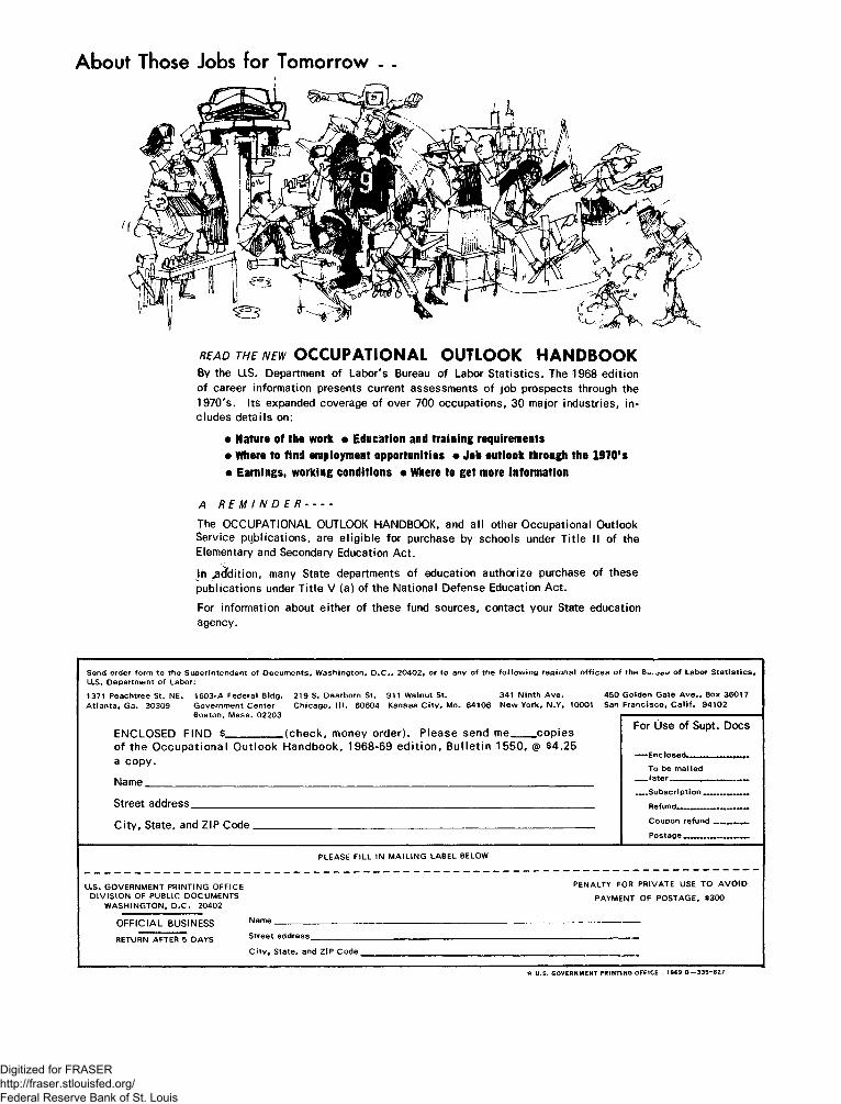
About Those Jobs for Tomorrow - -
READ THE NEW OCCUPATIONAL OUTLOOK HANDBOOKBy the US. Department of Labor's Bureau of Labor Statistics. The 19 6 8 edition of career information presents current assessments of job prospects through the 1 9 7 0 's. Its expanded coverage of over 7 0 0 occupations, 3 0 major industries, includes details on:
• Nature of the work • Education and training requirements• Where to find employment opportunities • Job outlook through the 1970’$• Earnings, working conditions • Where to get more information
A R E M I N D E R -----The OCCUPATIONAL OUTLOOK HANDBOOK, and all other Occupational Outlook Service publications, are eligible for purchase by schools under T itle II of the Elementary and Secondary Education Act.In ^adfdition, many State departments of education authorize purchase of these publications under T itle V (a) of the National Defense Education Act.For information about either of these fund sources, contact your State education agency.
Send order form to the Superintendent of Documents, Washington, D.C., 20402, or to any of the following regional offices of the Bu.^au of Labor Statistics* U.S. Department of Labor:1371 Peachtree St. NE. 1603-A Federal Bldg. 219 S. Dearborn St. 911 Walnut St. 341 Ninth Ave.Atlanta, Ga. 30309 Government Center Chicago, III. 60604 Kansas City, Mo. 64106 New York, N.Y. 10001
Boston, Mass. 02203
ENCLOSED FIN D $ v (check, money order). Please send me___ copiesof the Occupational Outlook Handbook, 1 9 6 8 -6 9 edition, Bulletin 1 5 5 0 , @ $4 .2 5 a copy.Name____________________________________________________________________Street address______________________________________________________________
450 Golden Gate Ave., Box 36017 San Francisco, Calif. 94102
For Use of Supt. Docs
—— E nc losed__To be mailed
.. . . later_______ ___ Subscription ....
Refund.__
C ity, State, and ZIP Code Coupon rqfundPostage ...
PLEASE FILL IN MAILING LABEL BELOW
U.S. GOVERNMENT PRINTING OFFICE DIVISION OF PUBLIC DOCUMENTS
WASHINGTON. D.C. 20402
OFFICIAL BUSINESS
RETURN AFTER 5 DAYS
Name___________________Street address___________City, State, and ZIP Code
PENALTY FOR PRIVATE USE TO AVOID PAYMENT OF POSTAGE. $300
☆ U.S. GOVERNMENT PRINTING OFFICE : 1969 0-335-827
Digitized for FRASER http://fraser.stlouisfed.org/ Federal Reserve Bank of St. Louis

Digitized for FRASER http://fraser.stlouisfed.org/ Federal Reserve Bank of St. Louis

Digitized for FRASER http://fraser.stlouisfed.org/ Federal Reserve Bank of St. Louis
U.S. DEPARTMENT OF LABOR BUREAU OF LABOR STATISTICS WASHINGTON, O.C. 20212
O F F I C I A L B U S I N E S S
POSTAGE AND FEES PAIDU.S. DEPARTMENT OF LABOR
i THIRD CLASS MAIL ii_________________________________________ ___________ i
Digitized for FRASER http://fraser.stlouisfed.org/ Federal Reserve Bank of St. Louis