Blood flow simulation and applications

Luisa Costa Sousa, Catarina F. Castro, and Carlos Conceição António

Abstract In the vascular system altered flow conditions, such as separation and flow-reversal zones play an important role in the development of arterial diseases. Nowadays computational biomechanics modeling is still in the research and de-velopment stage. This chapter presents a numerical computational methodology for blood flow simulation using the Finite Element method outlining field equa-tions and approaches for numerical solutions. Due to the complexity of the vascu-lar system simplifying assumptions for the mathematical modeling process are made. Two applications of the developed tool to describe arterial hemodynamics are presented, a flow simulation in the human carotid artery bifurcation and a search for an optimized geometry of an artificial bypass graft.

1.1 Introduction

Nowadays, the use of computational techniques in fluid dynamics in the study of physiological flows involving blood is an area of intensive research [1-4]. The mechanics of blood flow in arteries plays an important role in the health of indi-viduals and its study represents a central issue of the vascular research. Arterial diseases such as wall conditions may cause blood flow disturbances leading to clinical complications in areas of complex flow like in coronary and carotid bifur-cations or stenosed arteries. It is well established that once a mild stenosis is formed in the artery, biomechanical parameters resulting from the blood flow and stress distribution in the arterial wall contribute to further progression of the dis-ease. Although blood flow is normally laminar, the periodic unsteadiness or pulsa-tile nature of the flow makes possible the transition to turbulence when the artery diameter decreases and velocities increase. A detailed understanding of local he-modynamic environment, influence of wall modifications on flow patterns and long-term adaptations of the vascular wall can have useful clinical applications, especially in view of reconstruction and revascularization operations [5,6].

Flow visualization techniques and non-invasive medical imaging data acquisi-tion such as computed tomography, angiography or magnetic resonance imaging, make feasible to construct three dimensional models of blood vessels. Measuring techniques such as Doppler ultrasound have improved to provide accurate infor-mation on the flow fields. Validated computational fluid dynamics (CFD) models using data obtained by these currently available measurement techniques [7-9] can

2

be very valuable in the early detection of vessels at risk and prediction of future disease progression.

Hemodynamic finite element simulation studies have been frequently used to gain a better understanding of functional, diagnostic and therapeutic aspects of the blood flow. Three different issues are necessary during such study defining the following methodology:

1. Definition of suitable mathematical models - due to the complexity of the vascular system, a preliminary analysis aiming at introducing suitable simplifying assumptions in the mathematical modelling process is necessary. Obviously, dif-ferent kinds of simplifications are suitable for different vascular problems;

2. Pre-processing of clinical data - the suitable treatment of clinical data is cru-cial for the definition of a real geometrical model, taken from a patient. This as-pect demands geometrical reconstruction algorithms in order to achieve simulation in real vascular morphologies;

3. Development of appropriate numerical techniques - the geometrical com-plexity of the vascular system suggests the use of unstructured grids, in particular for Finite Element Method (FEM), while the strongly unsteady nature of the prob-lem demands effective time-advancing methods.

The arterial wall is a composite of three layers, each containing different amounts of elastin, collagen, vascular smooth muscle cells and extracellular ma-trix. In diseased vessels which are often the subject of interest, the arteries are less compliant, wall motion is reduced and in most approximations the assumption of rigid vessel flow is reasonable.

Blood consists of formed elements suspended in plasma, an aqueous polymer solution. About 45% volume consists of formed elements and about 55% of plas-ma. The majority of formed elements are red blood cells (95%). In large and me-dium size vessels, blood is usually modelled as a Newtonian liquid. However in smaller vessels blood is a complex rheological mixture showing several non-Newtonian properties, as shear-thinning or viscoelasticity. The temperature and the presence of pathological conditions may also contribute to non-Newtonian be-haviour.

For the steady flow case [10] showed that the non-Newtonian effect is small except for the peak shear stress and that for the pulsatile case the Newtonian effect in the artery is small and negligible. Perktold and co-workers examined non-Newtonian viscosity models in carotid artery bifurcation and although the Newto-nian assumption yields no change in the essential flow characteristics they con-cluded that predicted shear stress magnitude resulted in differences on the order of 10% as compared with Newtonian models [11].

A non-Newtonian viscosity model for simulating flow in arteries is presented in this chapter. Considering blood flow an incompressible non-Newtonian flow and neglecting body forces, the fluid flow is governed by the incompressible Navier-Stokes equations. There are two potential sources of numerical instability in the Galerkin finite element solution of these equations. The first one is due to the nu-merical treatment of the saddle-point problem arising from the variational formu-lation of the incompressible flow equations. The second difficulty is related to the

3

discretization of the nonlinear convective terms which requires the use of stabi-lized finite element formulations to properly treat high Reynolds number flows. Some of the approaches for the numerical solutions are presented in this study.

To demonstrate the application of the developed finite element technique for numerical simulations of blood flow in arteries, a flow simulation in the human carotid artery bifurcation and a search for an optimized geometry of an artificial bypass graft is addressed here. In medical practice, bypass grafts are commonly used as an alternative route around strongly stenosed or occluded arteries. When the arterial flow is high, artificial grafts perform well [2,12,13] and it has been shown over the years that they provide durable results. Su [2] investigated the complexity of blood flow in the complete model of arterial bypass. He found that flow in the bypass graft is greatly dependent on the area reduction in the host ar-tery. As the area reduction increases, higher stress concentration and larger recir-culation zones are formed bringing out the possibility of restenosis. Probst [14] concluded that computing derivatives of the flow solution (and related quantities like shear rate) with respect to viscosity could not reveal the sensitivity of the op-timal graft shape to the fluid model. So, optimization should be applied to the en-tire framework, which would enable to actually compute the optimal shape. In the present work a multi-objective optimization framework is presented. A genetic al-gorithm coupled with the developed finite element methodology for blood flow simulation is considered in order to reach optimal graft geometries. Numerical re-sults show the benefits of shape optimization in achieving design improvements before a bypass surgery, minimizing recirculation zones and flow stagnation.

1.2 Governing equations

A number of important phenomena in fluid mechanics are described by the Na-vier-Stokes equations. They are a statement of the dynamical effect of the exter-nally applied forces and the internal forces due to pressure and viscosity of the flu-id. The time dependent flow of a viscous incompressible fluid is governed by the momentum and mass conservation equations, the Navier-Stokes equations given as:

.

. 0

t

∂ + ∇ = ∇ + ∂

∇ =

uu u σ f

u

ρ (1)

where u and σ are the velocity and the stress fields, ρ the blood density and f

the volume force per unit mass of fluid. The components of the stress tensor are defined by the Stokes’ law:

2 ( )p= − +σ I ε uµ (2)

4

where p is the pressure, I the unit tensor, µ the dynamical viscosity and )ε(u the

strain rate tensor. Neglecting body forces, conservation of mass and momentum equations (1) become:

.

. 0

pt

∂ + ∇ = −∇ + ∇ ∂

∇ =

uu u u

u

ρ µ (3)

This equation system (Eq. (3)) can be solved for the velocity and the pressure given appropriate boundary and initial conditions. In this study the biochemical and mechanical interactions between blood and vascular tissue are neglected. The innermost lining of the arterial wall in contact with the blood is a layer of firmly attached endothelial cells and it appears to be reasonable to assume no slip at the interface with the rigid vessel wall; at the flow entrance Dirichelet boundary con-ditions for all points are considered prescribing the time dependent value Du for

the velocity on the portion DΓ of the boundary:

( ) ( ), , ,D Dt t= ∈Γu x u x x (4)

At an outflow boundary NΓ the condition describing surface traction forceh

is assumed. This can be described mathematically by the condition:

ij , 1,2,3 onji

j i Nj j

uup n h i j

x x

∂∂ − δ + + = = Γ

∂ ∂

µ (5)

where jn are the components of the outward pointing unit vector at the outflow

boundary.

1.3 Finite element formulation

The finite element method is a mathematical technique for obtaining approximate numerical solution of the physical phenomena subject to initial and boundary con-ditions. Two different finite element models of the Navier-Stokes equations are considered in this chapter, the mixed model and the penalty finite element model.

1.3.1 Mixed finite element model

The mixed model is a natural formulation in which the weak forms of Eq. (3) are used to construct the finite element method. The resulting finite element model is termed the velocity-pressure model or mixed model. Developing a Galerkin for-

5

mulation the weak forms of Eq. (3) results in the following finite element equa-tions:

.

T

=

− =

Mu+ C(u)u + Ku - QP F

Q u 0 (6)

where the superpose dot represents a time derivative. Considering N and L the el-ement interpolation functions for the velocity and pressure, the elements of the matrices at the finite element level are defined as:

;

;

j j jij i j ij i x y ze e

j j ji i i iij ik ke e

N N NM N N de C N u u u de

x y z

N N NN N N NK de Q L

x x y y z z

=

α

∂ ∂ ∂ = + + ∂ ∂ ∂

∂ ∂ ∂ ∂ ∂ ∂ ∂= µ + + = ∂ ∂ ∂ ∂ ∂ ∂ ∂α

∫ ∫

∫ ∫

ρ ρ (7)

and the resulting equation system is:

.

T

− + =

−

C + K Q u FMu

P 0Q 0 (8)

The above partitioned system (Eq. (8)) with a null submatrix could in principle be solved in several ways. However, it can be asked under which conditions it can be safely solved. This problem results from the incompressibility condition. In simple terms, we want to obtain, in the linear space U of all admissible solutions,

the velocity field u belonging to a subspace hI U⊂ , associated to the space of incompressible deformations. This subspace is given as:

:h h h hI U= ∈ =u Qu 0 (9)

The solution hI should then lie on the null space of Q that must be zero. The numerical problem described above is eliminated by proper choice for the finite element spaces of the velocity and pressure fields; in other words the evaluation of the integrals for the stiffness matrix where velocity and pressure interpolations ap-pear must satisfy the Babuska-Brezzi compatibility condition the so called LBB condition [15-17] that states velocity and pressure spaces can not be chosen arbi-trarily and a link between them is necessary.

In this chapter the numerical procedure for the transient non-Newton inelastic Navier-Stokes equations uses the Galerkin-finite element method with implicit time discretization. Considering a 3D analysis hexahedral meshes often provide

6

the best quality solution as errors due to numerical diffusion are reduced whenever a good alignment between mesh edges and flow exists [4]; in this work a spatial discretization with isoparametric brick elements of low order with trilinear ap-proximation for the velocity components and element constant pressure is adopt-ed:

and∑u x x8

i i ci=1

( ,t) = N ( )u (t) p(t) = Mp (t) (10)

where andi cu p are the unknown element velocity node values and the pressure

element center value, respectively. At each time step Picard iteration is applied to linearize the non-linear convection and diffusion terms; the method is based on a pressure correction [11,18]. The essential steps of the algorithm at a time or itera-tion are: 1. Calculation of an auxiliary velocity field from the equations of motion using known pressure values from the previous time step or previous iteration step; 2. Calculation of the pressure correction using lumped mass matrix; 3. Pressure updating; 4. Calculation of the divergence free velocity field; 5. Calculation of the apparent viscosity. This method developed for obtaining a divergence-free velocity field has been based on Chorin’s method [19] and validated by other authors.

1.3.2 Penalty finite element model

The incompressibility constraint given by 0iiε = is difficult to implement due to

the zero divergence condition for the velocity field. The incompressible problem may be stated as a constrained minimization of a functional. The penalty function method, like the Lagrange multiplier method, allows us to reformulate a problem with constraints as one without constraints [15,17]. Using the penalty function method proposed by Courant [20], the problem is transformed into the minimiza-tion of the unconstrained augmented functional:

( )( )2( ) ( ) dii

V

Vπ = π + λ∫u u uε (11)

Considering the pseudo-constitutive relation for the incompressibility con-straint the second set of Eq. (3) is replaced by:

. /p∇ = − λu (12)

7

where λ is the penalty parameter. If λ is too small compressibility and pressure errors will occur and an excessively large value may result in numerical ill condi-tioning; generally λ is assigned to λ = βµ being β a constant of order 107 for

double precision calculations. The second set of Eq. (3) is eliminated and the Na-vier-Stokes equations become:

( )λ.M u+ C + K + K u = F (13)

where λK is the so-called penalty matrix:

and pp pi jij e

M L L deλ = λ = λ = ∫t tK QM Q M P Q u (14)

Under such conditions the pressure is eliminated as a field variable since it can be recovered by the approximation of Eq. (12). If the standard Galerkin formula-tion is applied it is necessary to use compatible spaces for the velocity and the pressure in order to satisfy the LBB stability condition. This often excludes the use of the equal order interpolation functions for both fields. In order to avoid oscilla-tory results the numerical problem is eliminated by proper evaluation of the inte-grals for the stiffness matrix where penalty terms are calculated using a numerical integration rule of an order less than that required to integrate them exactly. This technique of under-integrating the penalty terms is known in the literature as the reduced integration.

1.3.3 Streamline upwind/Petrov Galerkin method

In a Galerkin formulation there is no doubt that the most difficult problem arises because of the nonlinear convective term in Eq. (3). In blood flow high Reynolds numbers appear and loss of unicity of solution, hydrodynamical instabilities and turbulence are caused by this apparently innocent term. The numerical scheme re-quires a stabilization technique in order to avoid oscillations in the numerical solu-tion. The most appropriate technique to solve these problems is the Streamline upwind/Petrov Galerkin method, SUPG-method [21,22]. The goal of this tech-nique is the elimination of the instability problems of the Galerkin formulation by introducing an artificial dissipation. The method uses modified velocity shape functions, iW , for the convective terms:

ii i SUPG

NW N K

∇= +

u

u (15)

8

where SUPGK denotes the upwind parameter that controls the factor of upwind

weighting. This parameter controls the amount of upwind weighting and is defined on an element as:

1

( ) , i=1,2,32

e e eSUPG i i ik Pe u h= ξ (16)

a function of eiu and e

ih element velocity and length, respectively, and the grid

Peclet number ePe . The SUPG-method produces a substantial increase in accura-cy as stabilizing artificial diffusivity is added only in the direction of the stream-lines and crosswind diffusion effects are avoided.

The resulting system of nonlinear equations is characterized by a non-symmetric matrix, and a special solver is adopted in order to reduce the bandwidth and the storage of the sparse system matrix; in addition the Skyline method is used to some improvement of the Gauss elimination.

1.3.4 Carotid bifurcation model

The numerical example presented here is a 3D flow simulation in the human ca-rotid artery bifurcation. Figure 1.1 shows the geometrical model described by Perktold [11,18]. The Navier-Stokes equations are solved using the Finite Element SUPG-method with implicit Euler backward differences for time derivatives and Picard iteration for nonlinear terms.

The non-Newtonian property of blood is important in the hemodynamic effect and plays a significant role in vascular biology and pathology. In this study the viscosity is empirically obtained using Casson law for the shear stress relation. Considering DII the second invariant of the strain rate and c the red cell concentra-tion, the shear stress τ given by the generalized Casson relation is:

0 1( ) 2 IIk k c D= +τ (17)

and the apparent dynamic viscosity µ = µ(c,DII), a function of the red cell concen-tration,

( )2

0 11

( ) 22

IIII

k k c DD

= +µ (18)

where parameters k0 = 0.6125 and k1 = 0.174 were obtained fitting experimental data, considering c = 45% and plasma viscosity µ0 = 0.124 Pa s [11].

The computer simulation is carried out under physiological pulsatile flow con-ditions. The considered time dependent flow rate waveform in the common carotid

9

and in the internal carotid arteries [11,23] is presented in Figure 1.2. The time-averaged flow rate in the common carotid is 5.1 ml/s and the mean common carot-id inflow velocity is U = 169 mm/s. In this work the common carotid diameter was taken equal to D = 6.2 mm (characteristic length), the reference blood viscosi-ty is µ = 0.0035 Pa s and the mean reference Reynolds number equal to Re =

300. At the inflow boundary fully developed time-dependent velocity profiles are

prescribed. The profiles correspond to the pulse waveform in the common carotid artery. At the rigid artery wall the no slip condition (u = 0) is applied. The condi-tions describing vanishing normal and tangential force of Eq. (5) cannot be ap-plied simultaneously at both outflow boundaries. The flow simulation is carried out in two steps. In the first calculation step, developed flow is assumed at the in-ternal carotid outlet according to the prescribed time-dependent flow division shown in Figure 1.2 and the condition of zero surface traction force is applied at the external carotid outflow boundary. During the second calculation step, which is the actual calculation step, the condition of zero surface traction force is applied at the internal carotid outflow boundary, while at the external carotid outflow boundary the results for the velocity profiles from the first step are used.

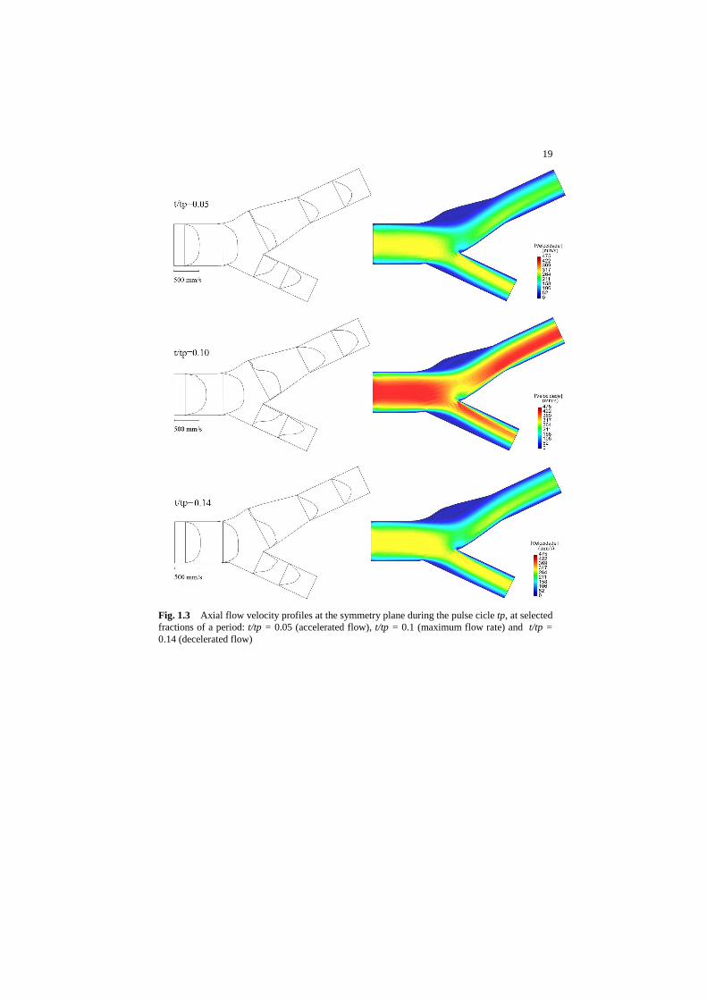
The flow characteristics in the carotid bifurcation are presented. Figure 1.3 shows velocity field during the pulse cicle tp, at selected fractions of a period: t/tp = 0.05 (accelerated flow), t/tp = 0.1 (maximum flow rate) and t/tp = 0.14 (deceler-ated flow). At the entrance of the internal and the external carotid relatively high axial velocities and steep velocity gradients can be observed near the divider wall. The shifting of the mass flow to the divider wall results from the branching effect and from the curvature effect. A zone of special hemodynamic relevance is the widened segment of the internal carotid, the carotid sinus. Time-dependent stag-nated and reversed flow occurs along the outer sinus wall (the wall opposite the divider wall). During systolic acceleration (t/tp = 0.05), only forward directed flow occurs in the sinus. At the end of flow acceleration (peak systole t/tp = 0.10) flow stagnation can be observed at the outer sinus wall near the entrance to the in-ternal carotid. During systolic deceleration (t/tp = 0.14 where the inflow rate is the same as at t/tp = 0.05) significant flow separation and reversed flow appear in the sinus. The reversed flow occupies around 50 percent of the sinus diameter in the branching plane.

The numerical findings on flow separation near the outer sinus wall agree with previously published results. In further studies the carotid bifurcation flow field will be investigated using parameters obtained from clinical observations.

1.4 Optimization of an artificial bypass graft

Numerical simulations of blood flow in arteries can be used to improve the under-standing of vascular diseases searching efficient treatments and medical devices. A framework for graft design optimization used in a bypass surgery, which is per-formed to restore blood flow in stenosed arteries is described here. Coupling shape

10

optimization to three-dimensional unsteady blood flow simulations poses several key challenges, including high computational cost, a need to handle constraints, and a need for automatic generation of parameterized vessel geometry. Instead, the applicability of the optimization framework is demonstrated considering a two-dimensional steady flow simulation. An idealized graft/artery model is pa-rameterized with a geometry allowing the analysis of the influence of graft-to-artery angle and diameter. Search for optimized arterial bypass grafts has been presented in the literature [12,14] always restricted to one objective function. This work represents the use of formal multi-objective optimization algorithms for sur-gery design.

1.4.1 Multi-objective optimization strategy

In shape optimization, the goal is to minimize an objective function that typically depends on a state vector u, over a domain of design vector b. The state vector and the design parameters are coupled by a partial differential equation that can be written in a generic form as

( , ) 0s =u b (19)

This so-called state equation forms the constraint of the minimization problem

Minimize ( , )

subject to ( , ) 0s

Φ=

u b

u b (20)

Furthermore, the problem can be recast using the reduced form of the objective function

*Minimize ( ( ), )Φ u b b (21)

where u(b) is the solution of Eq. (19). This form allows decoupling the solution of the state equation and the optimization problem.

A general multi-objective optimization seeks to optimize the components of a vector-valued objective function mathematically formulated as

1 2Minimize ( ) ( ( ), ( ),..., ( ))

subject to

mF f f f=

≤ ≤≤

b b b b

b

upperloweri i i

k

b b b , i = 1,...,n

g ( ) 0 , k = 1,..., p

(22)

where b = (b1,…,bn) is the design vector, bilower and bi

upper represent the lower and upper boundary of the ith design variable bi, fj(b) is the jth objective function and

11

gk(b) the kth constraint. Unlike single objective optimization approaches, the solu-tion to this problem is not a single point, but a family of points known as the Pare-to-optimal set. A Pareto optimal solution is defined as one that is not dominated by any other solution of the multi-objective optimization problem. Typically, there are infinitely many Pareto optimal solutions for a multi-objective problem. Thus, it is often necessary to incorporate user preferences for various objectives in order to determine a single suitable solution.

Genetic algorithms are well suited to multi-objective optimization problems as they are fundamentally based on biological processes which are inherently multi-objective.

1.4.2 Genetic search

A genetic algorithm (GA) is a stochastic search method based on evolution and genetics exploiting the concept of survival of the fittest. For a given problem or design domain there exists a multitude of possible solutions that form a solution space. In a genetic algorithm, a highly effective search of the solution space is per-formed, allowing a population of strings representing possible design vectors to evolve through basic genetic operators. The goal of these operators is to progres-sively reduce the space design driving the process into more promising regions.

Multi-objective genetic algorithms (MOGAs) were first suggested by Schaffer [24]. Since then several algorithms have been proposed on the basis of an evolu-tionary process searching for Pareto optimal solutions. MOGAs have been suc-cessfully applied to solve various kinds of multi-objective problems as they are not as much affected by nonlinearities and complex objective functions as mathe-matical programming algorithms.

One MOGA strategy consists of transferring multi-objectives to a single objec-tive by a weighted sum approach. The weighted sum method for multi-objective optimization problems continues to be used extensively not only to provide multi-ple solution points by varying the weights consistently, but also to provide a single solution point that reflects preferences presumably incorporated in the selection of a single set of weights. Using the weighted sum method to solve the optimization problem given in Eq. (22) entails selecting scalar weights wj and minimizing the following composite objective function:

*

1,

( ) ( )j jj m

F w f=

= ∑b b (23)

If all of the weights are positive, as assumed in this study, then minimizing Eq. (23) provides a sufficient condition for Pareto optimality, which means that its minimum is always Pareto optimal [25]. The weighting for an individual objective can be determined by either fixed weights or random weights. A strategy of ran-domly assigning weights is used to search for an optimum solution through di-

12

verse directions [26,27]. To provide decision makers with flexible and diversified solutions, this study adopts random weights calculated by using

1 2

, 1,...,...

jj

m

rw j m

r r r= =

+ + + (24)

where r j is a random positive integer. The genetic algorithm scheme searching for optimal solutions is based on four

operators supported by an elitist strategy that always preserves a core of best indi-viduals of the population whose genetic material is transferred into the next gener-ations [28,29]. A new population of solutions Pt+1 is generated from the previous Pt using the genetic operators: Selection, Crossover, Mutation and Deletion.

The optimization scheme includes the following steps: Coding: the design variables expressed by real numbers are converted to binary numbers, forming a string, and each binary string is looked as an individual; Initializing: the individuals which consist of an initial population P0 are produced randomly within each allowable interval; Evaluation: the fitness of each individual is evaluated using the objective function given in Eq. (23), and individuals are ranked according to their fitness value; Selection: definition of the elite group that includes individuals highly fitted. Se-lection of the progenitors is the mechanism that defines the process in which the chromosomes are mated before applying crossover on them. We apply a procedure that randomly chooses one parent from the best-fitted group (elite) and another from the least fitted one. Transfer of the whole population Pt to an intermediate step where they will join the offspring determined by the crossover operator; Crossover: One offspring per each pair of selected parents is considered in the present work. The value of each gene in the offspring chromosome coincides with the value of the same gene in one of the parents depending on a given probability. The new individuals created by crossover will join the original population. Mutation: the implemented mutation is characterized by changing a set of bits of the binary string corresponding to one variable of a randomly selected chromo-some from the elite group making possible the exploitation of previously un-mapped space design regions and guaranteeing the diversity of the generated pop-ulation. Deletion: After mutation, new ranking of the enlarged population according to their fitness. Then, it follows the deletion of the worst solutions with low fitness simulating the natural death of weak and old individuals. The original size popula-tion is recovered and the new population Pt+1 is obtained; the evolutionary process will continue until the stopping criterion is reached. Termination: checking the termination condition. If it is satisfied, the GA is termi-nated. Otherwise, the process returns to step Selection.

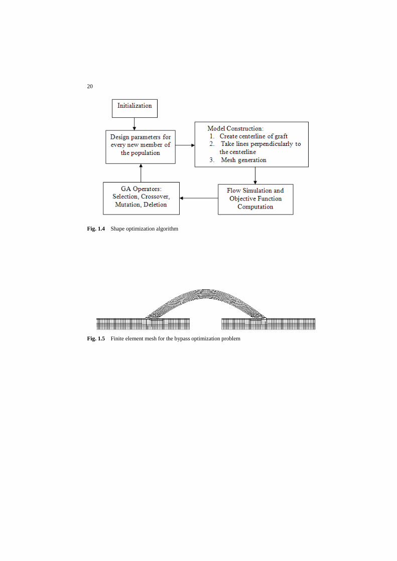
To fully automate the shape optimization procedure, the following sub-steps are linked in our framework: model generation, meshing, multi-objective function evaluation (flow simulation and post processing) and data transfer into the GA so

13

that the optimization procedure does not require any user intervention. Figure 1.4 shows the sub-steps of the optimization procedure. The boxes and arrows in Fig-ure 1.4 form a loop that repeats until stopping criteria are satisfied.

1.4.3 Optimized graft example

Search for an optimized geometry of an idealized arterial bypass system with fully occluded host artery is addressed here. This shape optimization problem requires an efficient and accurate solver for steady flow simulation. The Navier-Stokes equations are solved using the previously described penalty finite element model. The non-Newtonian behaviour of the blood is described using Casson law given by Eq. (18).

The objective functions need to be carefully chosen to capture the physics of the underlying problem. Regarding the choice of suitable objective functions for the graft optimization problem, several different approaches have been pursued in the literature [2,12,14]. The most frequently considered quantities in the context of blood flow are based on either shear stress and its gradient or the flow rate. Many authors choose to minimize the integral of the squared shear rate over the entire simulated domain ( )Ω b . This integral is also called dissipation integral because it

measures the dissipation of energy due to viscous effects, expressed in terms of the rate of strain tensor,

2.

( )

1

2dx

Ωγ∫ b

(25)

The minimization of this function is related to flow efficiency. Flow efficiency can equivalently be measured by computing the maximum pressure variation in the domain. In this project we chose to optimize the flow efficiency by minimizing the pressure variation quantified as:

1 max min( ) p p pϕ = ∆ = −b (26)

The second chosen objective function is related to the minimization of reversed flow and residence times along the arterial bypass system. For each idealized by-

pass graft geometry simulation, a domain * ( )Ω b has been identified indicating

where reversed flow and residence times are enhanced. Then, to minimize resi-dence times is equivalent to maximize the longitudinal velocity xu in that critical

domain. The following objective function is considered for the minimization prob-lem investigated in this work,

2* ( )

( ) x

Ω

ϕ = − ∑b

b u (27)

14

The artery is simulated using a fixed diameter tube of 10 mm. Design parame-ters are considered for the coupled graft presenting a sinusoidal geometry. The graft mesh does not maintain the same width along its whole length. At the centre line of the graft, nodes move in the radial direction preserving their distance to the deforming centreline. The graft is properly connected to the artery always in the same region but the graft diameter will vary. Due to the sinusoidal shape, the graft artery junction is always larger than the width at the graft center line.

The developed computer program modelled blood flow in artery and graft us-ing 2261 nodes and 2024 four-node linear elements for a two-dimensional finite element approximation. Figure 1.5 presents the geometry and finite element mesh considered for the idealized arterial bypass system simulation with the flow pro-ceeding from left to right. The boundary conditions for the flow field are parabolic inlet velocity corresponding to a Reynolds number equal to 300, no-slip boundary conditions including the graft and a parallel flow condition at the outlet.

For the optimization problem the graft/artery ratio diameter varies from 0.6 to 1.2, the height of the sinus curve varies from 10 to 20 mm and a circular anasto-mosis is set accordingly. Only symmetric geometries were considered since re-moving the symmetry constrain does not have a major effect [30]. So asymmetry is not requisite for the design of the bypass under the given flow conditions.

The search space is not known in absolute terms and simulations of 100 ran-dom possible graft designs have been conducted in order to get an indication of the objective space distribution. Figure 1.6 presents results for maximum pressure variation in the whole domain ( )Ω b and for the longitudinal velocity in the criti-

cal domain * ( )Ω b where reversed flow and residence times are enhanced. The

optimal solutions in the decision space are in general denoted as the Pareto set and its image in the objective space as Pareto front. Results shown in Figure 1.6 allow identifying the likely presence of a Pareto front in the design problem. The shape optimization will allow at least a 20% decrease on the pressure variation.

Since objective values are distributed in different ranges normalizing objective values by the fittest in the generation before the weighted-sum operation has been proposed [31]. For the optimization example, Eq. (23) becomes:

* 1 21 2* *

1 2

( ) ( )( )

( ) ( )F w w

ϕ ϕ= +

ϕ ϕb b

bb b

(28)

where *1ϕ and *

2ϕ are the fittest values for 1ϕ and 2ϕ , respectively, in the genera-

tion. The weight parameters w1 and w2 are random values calculated as in Eq. (24). The fitness function to be maximized by the GA is then defined as:

* ( )FIT A F P= − −b (29)

being A a positive integer to ensure positiveness and P a value to penalize design vectors that do not conform with constraints. As a compromise between computer

15

time and population diversity, parameters for the genetic algorithm were taken as Npop = 12 and Ne = 5 for the population and elite group size, respectively. The number of bits in binary codifying for the design variables was Nbit = 5. Optimal bypass geometries were obtained setting the maximum number of generations as 200. One optimal graft with design parameters given as graft diameter of 11.7 mm and height 18.7 mm is discussed here. The simulated longitudinal velocity values for the optimal graft solution are given in Figure 1.7. The longitudinal velocity distribution along bypass and host artery can be analysed in three parts. In the first part the flow is still undisturbed and therefore the velocity is quite uniform. In the second part the flow is within the graft area where the velocity raises as the flow moves along the graft. In the third part the flow is sufficiently far from the graft and therefore it exhibits a uniform distribution. At the exit of the graft after the ar-tery-graft junction, the velocity values variation is rather smooth. It is interesting to notice that although the abrupt connection between artery and graft induces large velocity variations, the observable reverse flow is quite small. Long resi-dence times usually observable immediately after the toe of the distal anastomosis are quite undetectable.

An optimal shape for idealized bypass graft geometry was obtained using a ge-netic search built around a developed finite element solver and adding routines evaluating objective functions. The solution exhibits the benefits of numerical shape optimization in achieving grafts inducing small gradient hemodynamic flows and minimizing reversed flow and residence times.

1.5 Concluding remarks

A computational finite element model for simulating blood flow in arteries is pre-sented. Blood flow is described by the incompressible Navier-Stokes equations and the simulation is carried out under steady and pulsatile conditions. The accu-racy and efficiency of the blood simulation is tested considering two examples. In the first example the finite element method is used to simulate blood flow in a ca-rotid artery bifurcation. Calculations of the flow field for the carotid artery are in good agreement with those reported previously in the literature. The model was able to simulate complex flow patterns in the carotid sinus like time-dependent stagnation and reversed flow along the outer sinus wall where flow separation oc-curs throughout the systolic deceleration phase.

The second example represents a step towards developing a formal optimiza-tion procedure for surgery design. An optimal shape for an idealized bypass is proposed. A major limitation of this study is the use of cylindrical models whereas parameterizations of patient specific models present significant challenges. Future work should also consider the influence of compliant walls and the effect of un-certainties in simulation parameters. Robust optimization that accounts for uncer-tainties could identify solutions that are less sensitive to small changes in design parameters, thus allowing a hospital surgical implementation.

Further studies will consider experimental data collected in clinical practice.

16

Acknowledgments This work was partially done in the scope of project PTDC/SAU-BEB/102547/2008, “Blood flow simulation in arterial networks towards application at hospital” , financially supported by FCT – Fundação para a Ciência e a Tecnologia from Portugal.

References 1. Pedrizzetti G., Perktold K.: Cardiovascular Fluid Mechanics. Springer-Verlag (2003) 2. Su, C.M., Lee, D., Tran-Son-Tay, R. & Shyy, W.: Fluid flow structure in arterial bypass

anastomosis. Journal of Biomechanical Eng. 127, 611-618 (2005) 3. Maurits N.M., Loots G.E., Veldman A.E.P.: The influence of vessel elaticity and peripher-

al resistance on the carotid artery flow wave form: A CFD model compared to in vivo ul-trasound measurements. Journal of Biomechanics 40, 427-436 (2007)

4. De Santis G, Mortier P, De Beule M, Segers P, Verdonck P, Verhegghe B.: Patient-specific computational fluid dynamics: structured mesh generation from coronary angiography.. Med. Biol. Eng. Comput. 2010 48(4), 371-80 (2010)

5. Taylor, C.A., Hughes, T.J.R. & Zarins, C.K.: Finite element modeling of blood flow in ar-teries. Comput. Methods Appl. Mech. Eng. 158, 155–196 (1998)

6. Quarteroni, A., Tuveri, M., Veneziani, A.: Computational Vascular Fluid dynamics: prob-lems,models and methods. Computer and Visualization in Science 2, 163-197 (2003)

7. Leuprecht A., Kozerke, S., Peter Boesiger, P. Perktold, K.: Blood flow in the human as-cending aorta: a combined MRI and CFD study. J. Eng. Math. 47(3), 387-404 (2003)

8. Kaazempur-Mofrad M.R., Isasi A.G., Younis H.F., Chan R.C., Hinton D.P., Sukhova G., LaMuraglia G.M., Lee R.T., Kamm R. D.: Characterization of the Atherosclerotic Carotid Bifurcation Using MRI, Finite Element Modeling and Histology. Annals of Biomedical Engineering 32(7), 932-946 (2004)

9. Schumann C., Neugebauer M., Bade R., Preim B., Peitgen H.-O.: Implicit vessel surface reconstruction for visualization and CFD simulation. Int. J. Computer Assisted Radiology and Surgery 2, 275–286 (2008)

10. Himeno R.: Blood Flow Simulation toward Actual Application at Hospital. The 5th Asian Computational Fluid Dynamics, Korea (2003)

11. Perktold, K., Resch, M., Florian, H.: Pulsatile Non-Newtonian Flow Characteristics in a Three-Dimensional Human Carotid Bifurcation Model. ASME J. Biomech. Eng. 113, 463–475. (1991)

12. Abraham F, Behr M, Heinkenschloss M.: Shape optimization in steady blood flow: a nu-merical study of non-Newtonian effects. Computer Methods in Biomechanics andBiomedi-cal Engineering; 8(2), 127–137 (2005)

13. Huang, H., Modi, V.J., Seymour, B.R.: Fluid mechanics of stenosed arteries. Int. J. Engng. Sci. 33, 815-828 (1995)

14. Probst M., Lülfesmann M., Bücker H. M., Behr M.,. Bischof C. H,: Sensitivity of shear rate in artificial grafts using automatic differentiation. Int. J. Numer. Meth. Fluids, 62, 1047–1062 (2010)

15. Babuska, I.: The finite element method with Lagrangian multipliers. Numer. Math. 20, 179-192 (1973)

16. Brezzi, F.: on the existence, uniqueness and approximation of saddle-point problems ar sing from Lagrangian multipliers. RAIRO Anal. Numér. 8(R2), 129-151 (1974)

17. Babuska, I., Osborn J., Pitkaranta J.: Analysis of mixed methods using, mesh dependent norms. Math. Comp. 35, 1039-1062 (1980)

18. Perktold, K., Rappitsch, G.: Mathematical modeling of local arterial flow and vessel me-chanics. In Crolet, J., Ohayon, R. (eds.) Computational Methods for Fluid Structure Inter-action. Pitman Research Notes in Mathematics 306, 230–245 Harlow: Longman (1995)

19. Chorin, A. J.:.Numerical solution of the Navier-stokes Equations. Math. Comp. 22, 745-762. (1968)

17

20. Courant R.: Variational methods for the solution of problems of equilibrium and vibration. Bull. Amer. Math. Soc. 49, 1- 23 (1943).

21. Hughes, T.J.R., Franca, L.P., Balestra, M.: A new finite element method for computational fluid dynamics: V. Circumventing the Babuska-Brezzi condition: A stable Petrov-Galerkin formulation of the Stokes problem accommodating equal order interpolations. Computer Methods in Applied Mechanics and Engineering 59, 85-99 (1986)

22. Hughes, T.J.R., Franca, L.P., Hulbert, G.M.: A new finite element method for computa-tional fluid dynamics: VIII The Galerkin/Least Squares method for advective diffusive equations. Computer Methods in Applied Mechanics and Engineering 73, 173-189 (1989)

23. Ku D.N., Giddens, D.P., Zarins, C.Z., Glagov, S.: Pulsatile flow and atherosclerosis in the human carotid bifurcation. Arterioscleresis 5, 293-302 (1985)

24. Schaffer, J.D.: Multi-objective optimization with vector evaluated genetic algorithms. Pro-ceedings of the 1st International Conference of Genetic Algorithms, 93–100 (1985

25. Marler, R.T., Arora, J.S.: The weighted sum method for multi-objective optimization: new insights. Struct. Multidisc. Optim. (2009). DOI 10.1007/s00158-009-0460-7

26. Kim, I.Y., Weck, O.L.de: Adaptive weighted sum method for multiobjective optimization: a new method for Pareto. Structural and Multidisciplinary Optimization 31, 105-116 (2006)

27. Coello, C.A.C., Lamont, G.B., and Veldhuizen, D.A.V.: Evolutionary algorithms for solv-ing multi-objective problems. Springer, NY (2007)

28. António, C.C., Castro, C.F., Sousa, L.C.: Eliminating forging defects using genetic algo-rithms. Materials and Manufacturing Processes 20, 509-522 (2005)

29. Castro, C.F., António, C.A.C., Sousa, L.C.: Optimisation of shape and process parameters in metal forging using genetic algorithms. Journal of Materials Processing Technology 146, 356-364 (2004)

30. Probst M., Lülfesmann M., Nicolai M., Bücker H. M., Behr M.,. Bischof C. H,: Sensitivity of optimal shapes of artificial grafts with respect to flow parameters. Comput. Methods Appl. Mech. Engrg., 199, 997-1005 (2010)

31. Cochran, J.K., Horng, S., Fowler, J.W.: A multi-population genetic algorithm to solve mul-ti-objective scheduling problems for parallel machines. Computers and Operations Re-search, 30, 1087-1102 (2003)

18

Fig. 1.1 Carotid artery bifurcation model

Fig. 1.2 Flow pulse waveform in the common carotid and in the internal carotid arteries

19

Fig. 1.3 Axial flow velocity profiles at the symmetry plane during the pulse cicle tp, at selected fractions of a period: t/tp = 0.05 (accelerated flow), t/tp = 0.1 (maximum flow rate) and t/tp = 0.14 (decelerated flow)

20

Fig. 1.4 Shape optimization algorithm

Fig. 1.5 Finite element mesh for the bypass optimization problem

21

Fig. 1.6 Maximum pressure variation and longitudinal velocities for critical domain

Fig. 1.7 Velocity distribution [mm s-1] for the optimal shape