HAL Id: hal-00409446https://hal.archives-ouvertes.fr/hal-00409446v4

Preprint submitted on 5 Jul 2010

HAL is a multi-disciplinary open accessarchive for the deposit and dissemination of sci-entific research documents, whether they are pub-lished or not. The documents may come fromteaching and research institutions in France orabroad, or from public or private research centers.

L’archive ouverte pluridisciplinaire HAL, estdestinée au dépôt et à la diffusion de documentsscientifiques de niveau recherche, publiés ou non,émanant des établissements d’enseignement et derecherche français ou étrangers, des laboratoirespublics ou privés.

Blood-flow modelling along and through a braidedmulti-layer metallic stent

Vuk Milisic

To cite this version:Vuk Milisic. Blood-flow modelling along and through a braided multi-layer metallic stent. 2009.hal-00409446v4

BLOOD-FLOW MODELLING ALONG AND TROUGH A BRAIDED

MULTI-LAYER METALLIC STENT ∗

VUK MILISIC†

Abstract. In this work we study the hemodynamics in a stented artery connected either to a collateral arteryor to an aneurysmal sac. The blood flow is driven by the pressure drop. Our aim is to characterize the flow-rate andthe pressure in the contiguous zone to the main artery: using boundary layer theory we construct a homogenizedfirst order approximation with respect to ǫ, the size of the stent’s wires. This provides an explicit expression of thevelocity profile through and along the stent. The profile depends only on the input/output pressure data of theproblem and some homogenized constant quantities: it is explicit. In the collateral artery this gives the flow-rate. Inthe case of the aneurysm, it shows that : (i) the zero order pressure inside the sac is equal to the averaged pressurealong the stent in the main artery, (ii) the presence of the stent inverses the rotation of the vortex. Extendingthe tools set up in [5, 27] we prove rigorously that our asymptotic approximation of velocities and pressures isfirst order accurate with respect to ǫ. We derive then new implicit interface conditions that our approximationformally satisfies, generalizing our analysis to other possible geometrical configurations. In the last part we providenumerical results that illustrate and validate the theoretical approach.

AMS subject classifications. 76D05, 35B27, 76Mxx, 65Mxx

Key words. wall-laws, porous media, rough boundary, Stokes equation, multi-scale modeling, boundary layers,pressure driven flow, error estimates, vertical boundary correctors, blood flow, stent, artery, aneurysm

1. Introduction. Atherosclerosis and rupture of aneurysm are lethal pathologies of thecardio-vascular system. A possible therapy consists in introducing a metallic multi-layered stent(see fig. 1.1 right). This device slows down the vortices in the aneurysm and doing so favorscoagulation of the blood inside the sac. This, in turn, avoids possible rupture of the sac.

In this study we aim to investigate the fluid-dynamics of blood in the presence of a stent.We focus on two precise configurations in this context: (i) a stented artery is connected to thecollateral artery but the aperture of the latter is partially occluded by the presence of the stent(see fig. 1.1 left), (ii) a sacular aneurysm is present behind a stented artery (fig. 1.1 middle).From the applicative point of view these two situations are of interest since they represent a dual

artery walls

blood−flow

stent’s wires

Figure 1.1. A sketch of stented arteries: with a collateral artery (left), an aneurysmal sac (middle) and a3D example of a real metallic multi-wired stent (right)

constraint that a stent should optimize somehow: the grid generated by the wires should be coarseenough to provide blood to the collateral arteries (for instance iliac arteries in the aorta), at thesame time the wires should be close enough to have a real effect in terms of velocity reduction inthe aneurysm.

∗ This research was partially funded by Cardiatis (www.cardiatis.com), an industrial partner designing andcommercializing metallic wired stents. This work was supported by a grant from Institut des Systemes Complexes(IXXI, www.ixxi.fr)

†Wolfgang Pauli Institute (WPI), UMI CNRS 2841,Vienna, AUSTRIA, (vuk.milisic@imag.fr)

1

Multi-layer metallic wired stents seem to satisfy both the constraints at the same time. Al-though experimentally exhibited [4, 26], these facts needed a better mathematical understanding.We give here results in this sense, setting a common framework for both phenomena in the caseof the Stokes flow.

Inspired by homogenization techniques applied to the case of rough boundaries [1, 22, 29] weconstruct a first-order multi-scale approximation of the velocity and the pressure. By averaging, weget a first order accurate macroscopic description of the fluid flow. Indeed, we compute an explicitexpression of the velocity through the fictitious interface supporting the stent and separating themain artery from the contiguous zone. This formula only depends on the input data of the problemand some homogenized constants obtained solving microscopic cell problems. In the case of theaneurysmal sac we show rigorously that the zero order pressure in the sac is constant and averagedwith respect to the pressure in the main artery, which was not known. Then we show that formallythis leads also to redefine the problem in a new and implicit way in the domain decompositionflavor. Actually we obtain a new set of interface conditions along the fictitious interface: whilefor the normal velocity they look similar to those presented in [10, 2, 9], the tangential conditionsare new to our knowledge. They express a slip velocity in the main artery (as in [20]), but adiscontinuous homotetic relationship between horizontal velocities across the interface of the stent(see system (3.4)). Our results concern the steady Stokes equations, as in [2], the same interfaceconditions are valid in the case unsteady Navier-Stokes case.

From the mathematical point of view this paper introduces several novelties. The case of asieve has been widely studied in a different setting in [11, 12, 2, 9, 6]. In these works, the authorsconsidered no-slip obstacles set on a surface with various dimensionalities but with a commonpoint: the velocity was completely imposed at the inlet/outlet boundaries of the fluid domain.Although this could seem a technicality, it influences drastically the limiting regime of the flow.Indeed a complete velocity profile is imposed as a Dirichlet condition at the inlet/outlet of thedomain, so that the total flow-rate through the sieve remains constant whatever ǫ, the size of theobstacles: a resistive term appears as a zeroth order limit in the fluid equations. In the context ofblood flow such a regime seems hard to reach: experiences show that when the wires are to denseno transverse flow crosses the stent. This suggests that through the porous interface, blood flowshould be driven by a pressure drop more that a fixed flow-rate.

In this direction, Jager and Mikelic considered a pressure driven fluid in [19]. But they studiedan interface whose thickness was independent on ǫ, which seemed useless for our purpose : thediameter of the wires of the stent are dependent on the radius of the artery where the stent shouldbe implanted. It appears natural to consider roughness size that varies wrt ǫ in any direction.Moreover in this paper we introduce both a tangential and a transverse flow along and troughthe stent. Indeed, in the limiting regime considered by Jager and Mikelic [19], the velocity iszero. Here when the collateral artery or a sac are completely closed by the stent, we still expecta Poiseuille profile in the main artery.

At a more technical level, this work improves the approach developed in [5, 27] in order tocorrect edge oscillations introduced by periodic boundary layers. At the same time, we give anappropriate framework to deal with this problem in the case of Stokes equations. Indeed, due tothe presence of the obstacles, the divergence operator is singular wrt ǫ, this implies degradationof convergence results when lifting the non-free divergence terms and estimating the pressure. Inthis frame, we decompose the corrections of the superfluous boundary layer oscillations in twoparts :

• on the microscopic side we use weighted Sobolev spaces to describe the behaviour atinfinity of the vertical corner correctors, defined on a half plane. This provides accuratedecay rates with respect to ǫ at the macroscopic level near the corner. Indeed, using ontomappings between weighted Sobolev spaces we improve decay estimates already derived inthe scalar case in [5, 27]. Then in the spirit of [2] we construct a microscopic lifting operatorthat allows the vertical correctors to fullfil the Dirichlet condition on the obstacles,

• a complementary macroscopic corrector is added in a second step, that handles exponen-tially decreasing errors far from the corners.

An attempt to break the periodicity at the inlet/outlet of the domain was done in [20] by using a

2

vertical corrector localized in a tiny strip near the vertical interface. But, decay estimates claimedin formula (77) p. 1123 [20] seem to work, to our knowledge, only for a priori estimates of theerror and are not accurate enough to be used in the very weak estimates.

We underline as well that in the literature [20, 21, 22, 23] error estimates between the directrough solution and the approximations constructed thanks to boundary layer arguments concernedthe L2 norm of the velocity. In this paper we provide error estimates of the same order for thepressure as well in the negative Sobolev H−1 norm. This is obtained using the microscopic natureof the pressure correctors and in particular thanks to the very precise control of lateral correctors.We stress that these vertical correctors play a crucial part in our error analysis at several steps ofthis work.

The paper is organized as follows: in the two next sections, after some basic notations anddefinitions, we give a detailed review of the results obtained either in the case of a collateral arteryor a sacular aneurysm. We give in section 4 the abstract results that are used in section 5 inorder to prove the claims. We provide numerical results showing a first order accuracy also in thediscrete case in section 6. In Appendix A, we give proofs of existence, uniqueness and a prioriestimates for vertical correctors in the weighted Sobolev spaces, while in Appendix B we detailthe results claimed for the periodic boundary layers throughout the paper.

2. Geometry and problem settings.

2.1. Geometry. In this study we consider two space dimensions. Let us define by Js oneor more solid obstacles included in J :=]0, 1[2 of Lipschitz boundaries denoted P in the sense ofthe definition p. 13-14 of Chap. 1 in [28]. We denote by Jf :=]0, 1[2\Js the complementary fluidpart of Js in ]0, 1[2. Also, we consider a smooth surface γM strictly contained in Js and enclosingP and we denote JM the domain contained between γM and P . Then we define:(i) Macroscopic domains:

The ǫ-periodic repetition of Jf is denoted by Lǫ and reads:

Lǫ := ∪mi=0ǫ((i, 0) + Jf ), where m :=

1

ǫ,

the real ǫ is always chosen such that m is an integer. Then we set:

Ω1 :=]0, 1[2, Γin := 0×]0, 1[,

Ω′1 :=]0, 1[×]ǫ, 1[, Γout,1 := 1×]0, 1[,

Ω1,ǫ := Ω′1 ∪ (]0, 1[×ǫ) ∪ Lǫ, Γout,2 :=]0, 1[×−1,

Ω2 :=]0, 1[×]− 1, 0[, Γ1 :=]0, 1[×1,Γ0 :=]0, 1[×0, Γ2 := 0×]− 1, 0[∪1×]− 1, 0[,

Ω := Ω1 ∪ Γ0 ∪ Ω2, ΓD := Γ1 ∪ Γ2 ∪ Γǫ,

Ωǫ := Ω1,ǫ ∪ Γ0 ∪Ω2, ΓN := Γin ∪ Γout,1 ∪ Γout,2,

Ω′ := Ω′1 ∪ Ω2, Eǫ :=]0, 1[×]0, ǫ[.

The spatial variable giving the position of a point in domains above is a vector called x.(ii) The microscopic cell domain:

As the problem contains a solid interface surrounded by a fluid, the microscopic cell problemsare set on an infinite strip Z defined as follows

Z− :=]0, 1[×]−∞, 0[,

Σ :=]0, 1[×0,Z+ :=]0, 1[×R+ \ Js,

Z := Z+ ∪ Σ ∪ Z−,

Zγ,ν := Z∩]0, 1[×]γ, ν[, (γ, ν) ∈ R2 s.t. γ < ν.

The microscopic position variable is denoted by y := x/ǫ.

3

(iii) The “corner” microscopic domain:In order to handle periodic perturbations on the lateral boundaries Γin∪Γ2∪Γout,1 one needsto define a microscopic zoom near the corners O := (0, 0) and x := (1, 0) of Ωǫ. This leadsto set the half-plane Π and the corresponding boundaries as

Π := R+ × R

N := 0×]0,+∞[,

D := 0×]−∞, 0[,

If we choose the obstacle Js to be a single disk, then a graphical illustration depicts the definitionsabove in fig. 2.1 for ǫ = 1/11.

Γin

Γ1

Γ2

Γǫ

Γout,2

Γ0

Ω1,ǫ

Ω2Γ2

Γout,1 Γin

Γ1

Γ2

Γout,2

Γ0

Ω1

Ω2Γ2

Γout,1

Z−

Js

Z+

Σ

P

JM

γM

Figure 2.1. The macroscopic domains Ωǫ (left) and Ω (middle) and the microscopic infinite strip Z (right)

The exterior normal vector to any domain is denoted by n, if not stated explicitly n is orien-tated from Ω1 towards Ω2 on the fictitious interface Γ0. The tangent vector is defined as τ .

2.2. Notations and definitions.

(i) Any two-dimensional vector is denoted by a bold symbol: u := (u1, u2), and single com-ponents are scalar and are not bold. The same holds for the function spaces these vectorsbelong to: bold letters denote vector spaces, for instance L2(Ω) := (L2(Ω))2.

(ii) If η ∈ H1loc(Z) then we set

η(y2) :=

∫ 1

0

η(y1, y2)dy1, y2 ∈ R,

to be the horizontal average of a function defined on the infinite periodic strip Z. Moreoverby the double bar we denote a piecewise constant function defined on Z as

η(y) := η(+∞)1Z+(y) + η(−∞)1Z−(y), y ∈ Z,

whenever the function η(·) admits finite limits when |y2| → ∞. We need the values of theabove function near the origin, thus we set also:

η±:= η(0±).

(iii) For any pair (u, p) ∈ L2(Ω) × H−1(Ω) we denote by σu,p the 2 × 2 distributional matrixreading

σu,p(x) := ∇u− pId2, a.e. x ∈ Ω,

where Id2 is the identity matrix in R2. The tensor σu,p looks like the stress tensor but it isnot symmetric. This is due to the incompressibility constraint: the Stokes problem can stillbe put in the divergence form with the definition of σu,p above.

4

(iv) The brackets [·] denote throughout the whole paper the jump of the quantity enclosed acrossfictitious interfaces: across Γ0 on the macroscopic scale, or across Σ on the microscopic scale,so that for instance

[σu,p] := σu,p(x1, 0+)− σu,p(x1, 0

−), while [η] := η+ − η

−.

(v) For every microscopic function η defined on either Z or Π, we denote by

ηǫ(x) = η(x

ǫ

)

, ∀x ∈ Ωǫ.

We also need cut-off functions that we define here:(vi) The cut-off φ is a scalar function φ : R+ → [0, 1] s.t. φ is a C∞(R+) monotone decreasing

function and

φ(z) :=

1 if z ≤ 1,

0 if z ≥ 2,

for any positive real z.(vii) The “corner” cut-off functions : set ψ1 := ψ(x) and ψ2 := ψ(x−x) and ψ is a radial monotone

decreasing cut-off function such that

ψ(x) :=

1 if |x| ≤ 1

3,

0 if |x| ≥ 2

3,

∀x ∈ R2.

Finally set ψ(x) := ψ1(x) + ψ2(x). Note that with this definition ∂nψ = 0 on Γin ∪ Γout,1.(viii) The “far from the corner” cut-off function : Φ is defined in a complementary manner on

Γin ∪ Γout,1 ∪ Γ2 such that

ψ +Φ = 1, on Γin ∪ Γout,1 ∪ Γ2,

∂nΦ = 0 on Γin ∪ Γout,1,

and one shall take for instance Φ(x) := 1− ψ(0, x2) for all x in Ω.(ix) For regularity purposes we set λǫ to be a cut-off function in the ǫ-neighborhood of the corners

O and x (p. 1122 [20]). First we set at the microscopic level:

λ(y) := |y2|1B(O,1)(y) +y2|y|1Π\B(O,1)(y), ∀y ∈ Π,

then we define

λǫ(x) := λ(x

ǫ

)

ψ1(x) + λ

(

1− x1ǫ

,x2ǫ

)

ψ2(x) + Φ(x), ∀x ∈ Ω.

and an easy computation shows that

‖λǫ‖H1(Ω) ≤ k| log(ǫ)| 12 + 1, (2.1)

where the constant k does not depend on ǫ.

3. Main results.

3.1. The case of a collateral artery. We study the problem : find (uǫ, pǫ) solving thestationary Stokes equations

−∆uǫ +∇pǫ = 0 in Ωǫ,

divuǫ = 0 in Ωǫ,

pǫ = pin on Γin, pǫ = pout,1 on Γout,1, pǫ = pout,2 on Γout,2,

uǫ · τ = 0 on Γin ∪ Γout,1 ∪ Γout,2,

uǫ = 0 on Γ1 ∪ Γ2 ∪ Γǫ,

(3.1)

5

Because of the microscopic structure of Γǫ, the solution of such a system is complex and expensivefrom the numerical point of view. For this reason throughout this article we use homogenizationin order to construct approximations of (uǫ, pǫ). This technique decomposes in two steps :1) the derivation of a multi-scale asymptotic expansion and the construction of an averaged macro-

scopic approximation. The first part can be seen as an iterative algorithm with respect topowers of ǫ :(a) pass to the limit with respect to ǫ and obtain a macroscopic zero order approximation.

In our case, because of the straight geometry of the main artery and of the boundaryconditions, the Poiseuille profile is obtained in Ω1 and a trivial solution in Ω2 :

u0(x) =pin − pout,1

2(1− x2)x2e11Ω1 ,

p0(x) = (pin(1 − x1) + pout,1x1)1Ω1 + pout,21Ω2 ,∀x ∈ Ω, (3.2)

(b) construct microscopic boundary layers correcting errors made by the zeroth order approx-imation on Γǫ and Γ0: we set up in the next section three boundary layers (β, π), (Υ, )and (χ, η) to this purpose. These functions solve periodic microscopic problems (5.2),(5.3) and (5.4) on the strip Z.

(c) compute the constants that these correctors reach at y2 = ±∞: (β±, 0), (Υ

±, 0) and

(χ, η±). Then subtract them to the correctors. Physically, β

±,Υ

±provide a microscopic

feed-back relative to the horizontal velocity (see the wall-law framework in [29, 20] andreferences therein) whereas the pressure difference [η] represents a microscopic resistivityin the flavor of [2, 9, 6].

(d) take into account the homogenized constants on the limit interface Γ0 by solving a macro-scopic problem: find (u1, p1) s.t.

−∆u1 +∇p1 = 0 in Ω1 ∪ Ω2,

divu1 = 0 in Ω1 ∪ Ω2,

u1 = 0 on Γ1 ∪ Γ2,

u1 · τ = 0

p1 = 0

on ΓN ,

u1(x1, 0±) =

(

∂u0,1∂x2

(x1, 0+)β

±

1 +

[

∂u0,1∂x2

]

Υ±

1

)

e1 +[p0]

[η]χ2e2 on Γ0

±

(3.3)

This macroscopic corrector depends on the zeroth order approximation and the homog-enized constants. Due to the explicit form of the Poiseuille profile, the Dirichlet datais explicit on both sides of Γ0, (nevertheless the solution (u1, p1) is not explicit insideΩ1 ∪Ω2).

(e) go to (1b) and correct, on a micrscopic scale, errors made by (u1, p1) on Γǫ ∪ Γ0 in orderto get higher order terms in the asymptotic ansatz.

2) The second step consists then in averaging this ansatz and obtaining an expansion of themacroscopic solutions only. This gives, for instance, at first order :

uǫ(x) := u0(x) + ǫu1(x), pǫ(x) := p0(x) + ǫp1(x), ∀x ∈ Ω1 ∪ Ω2.

In particular as uǫ · n = ǫ[p0]/[η] on Γ0, one gets an explicit first order velocity profile acrossΓ0. As a consequence, we obtain a new result :Proposition 1. The flow-rate in the collateral artery Ω2 can be computed explicitly and reads

QΓ0 :=

∫

Γ0

uǫ · ndx1 =ǫ[

η]

∫

Γ0

[p0]dx1 =ǫ[

η]

∫

Γ0

(pout,1 + (pin − pout,1)(1 − x1)− pout,2) dx1

As stated above [η] depends only on the geometry of the microscopic obstacle Js and isindependent of any other parameter. In the last section of this paper we give some numerical

6

examples that illustrate the accuracy of this result (see fig. 6.5 and 6.6). Note that the zerothorder approximation does not provide any transverse flow through Γ0. Although our resultsprovide a first order correction, we underline that in the physiological context the pressures(pin, pout,1) present in the main artery can be very important compared to pout,2 : the firstorder flow rate QΓ0 can thus be quantitatively significant as well.In this work we constructed an suitable mathematical framework in order to analyse the error

made in the two main steps of the construction above. This allows to state the main result of thispaper:

Theorem 3.1. There exists a unique pair (uǫ, pǫ) ∈ H1(Ωǫ)× L2(Ωǫ) solving problem (3.1).The averaged asymptotic ansatz (uǫ, pǫ) belongs to L2(Ωj) ×H−1(Ωj) for j ∈ 1, 2 and satisfiesthe convergence result

‖uǫ − uǫ‖L2(Ω1∪Ω2)+ ‖pǫ − pǫ‖H−1(Ω′

1∪Lǫ∪Ω2)≤ kǫ

32−

,

where 32

−represent any real number strictly less then 3

2 and the constant k is independent on ǫ.Expressing interface conditions satisfied by (uǫ, pǫ) on Γ0 in an implicit way and neglecting

higher order rests, we show formally that in fact (uǫ, pǫ) solve at first order a new interfaceproblem :

−∆uǫ +∇pǫ = 0 in Ω1 ∪Ω2,

divuǫ = 0 in Ω1 ∪Ω2,

uǫ = 0 on Γ1 ∪ Γ2,

uǫ · τ = 0 on ΓN ,

pǫ = pin, on Γin, pǫ = pout,1 on Γout,1, pǫ = pout,2 on Γout,2,

u+ǫ · τ = ǫ(β

+

1 +Υ+

1 )∂uǫ,1∂x2

+

,u+ǫ · τ

β+

1 +Υ+

1

=u−ǫ · τ

β−

1 +Υ−

1

u+ǫ · n = u−

ǫ · n = − ǫ

[η]([σuǫ,pǫ

] · n,n)

on Γ0.

(3.4)

The horizontal velocity on Γ0+ is related to the shear rate trough a kind of mixed boundary

condition alike to the Beaver, Joseph and Saffeman condition [20]. This implicit relationshipaccounts for the friction effect due to the obstacles that “resist” to the flow in the main artery.Nevertheless because the interface separates two domains Ω1 and Ω2, we obtain a second expressionbetween the upper and the lower horizontal velocities u+ǫ,1 and u−ǫ,1: they are proportional andthus discontinuous. To our knowledge this is new.

On the other hand, the interface condition on the normal velocity could be integrated in theStokes equations as a kind of “strange term” in the spirit of [10, 2], but as we are at first order withrespect to ǫ: (i) the strange term is divided by ǫ (in [10, 2] this is a zero order term independenton ǫ ) (ii) the derivation does not follow at all the same argumentation. In a forthcoming work westudy the well-posedness of such a system as well as its consistency with respect to (uǫ, pǫ) and(uǫ, pǫ). Because of the particular signs of the homogenized constants but also the discontinuousnature of the interface conditions in the tangential direction to Γ0, this seems a challenging task.

3.2. The case of an aneurysm. The framework introduced above can be extended to thecase of an aneurysm; considering the same domain Ωǫ as above we define a new problem : find(uǫ, pǫ) solving

−∆uǫ +∇pǫ = 0 in Ωǫ,

divuǫ = 0 in Ωǫ,

pǫ = pin on Γin, pǫ = pout,1 on Γout,1,

uǫ · τ = 0 on Γin ∪ Γout,1,

uǫ = 0 on Γ1 ∪ Γ2 ∪ Γout,2.

(3.5)

7

The main difference resides in the boundary condition imposed on Γout,2 : here we impose acomplete adherence condition on the velocity ; this closes the output Γout,2 and transforms thecollateral artery into an idealized square aneurysm.

Again, we construct a similar multi-scale asymptotic ansatz. We extract the macroscopic partto get a homogenized expansion (uǫ, pǫ) reading

uǫ(x) := u0(x) + ǫu1(x), pǫ(x) := p0(x) + ǫp1(x), ∀x ∈ Ω1 ∪ Ω2,

where (u0, p0) is again a Poiseuille profile but complemented by an unknown constant pressure p−0inside the sac:

u0(x) =pin − pout,1

2(1− x2)x2e11Ω1

p0(x) = p+0 (x)1Ω1 + p−0 1Ω2 ,

p+0 (x) := pout,1 + (pin − pout,1)(1 − x1), p−0 ∈ R

, ∀x ∈ Ω (3.6)

Then again (u1, p1) solves a mixed Stokes problem (3.3), the only difference being that u1 = 0 onΓout,2. This gives again a new result:

Corollary 3.1. The zeroth order pressure is constant in Ω2, moreover it satisfies the fol-lowing compatibility condition with respect to the pressure in the main artery:

p−0 =1

|Γ0|

∫

Γ0

p+0 (x1, 0) dx1.

This gives an explicit velocity profile on Γ0 which reads:

uǫ · n =ǫ

[η](p+0 (x1, 0)− p−0 ) +O(ǫ2).

The interface condition exhibited on the normal velocity shows rigorously a phenomenonalready observed experimentally [4, 26]. Set x1,max := maxx∈Γ0 x1 (resp. x1,min := minx∈Γ0 x1)and x1 := (x1,max + x1,min)/2, when x1 < x1 the pressure jump [p0] := p+0 (x) − p−0 is positive,otherwise it is negative. This implies that the first order flow trough the stent is entering Ω2 whenx1 < x1 and leaving it otherwise. Thus the prosthesis inverses the orientation of the cavitation inΩ2 with respect to the non-stented artery (see fig. 3.1).

Figure 3.1. Streamlines and velocity vectors in an aneurysmal sac, with (left) and without a stent (right)

As stated in the corollary, we show in the next section that in fact the zero order pressure isthe only constant that insures conservation of mass in Ω2. From the medical point of view thetwo claims on pressure and flow are of interest. They quantify and confirm the stabilizing effectof a porous stent: besides reducing the stress on the wall of the aneurysm,the stent averages alsothe pressure inside the sac avoiding for instance corner singularities (see fig. 3.2).

8

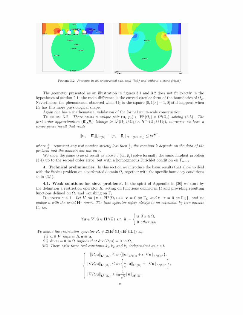
Figure 3.2. Pressure in an aneurysmal sac, with (left) and without a stent (right)

The geometry presented as an illustration in figures 3.1 and 3.2 does not fit exactly in thehypotheses of section 2.1: the main difference is the curved circular form of the boundaries of Ω2.Nevertheless the phenomenon observed when Ω2 is the square ]0, 1[×]− 1, 0[ still happens whenΩ2 has this more physiological shape.

Again one has a mathematical validation of the formal multi-scale constructionTheorem 3.2. There exists a unique pair (uǫ, pǫ) ∈ H1(Ωǫ) × L2(Ωǫ) solving (3.5). The

first order approximation (uǫ, pǫ) belongs to L2(Ω1 ∪ Ω2) × H−1(Ω1 ∪ Ω2), moreover we have aconvergence result that reads

‖uǫ − uǫ‖L2(Ω) + ‖pǫ − pǫ‖H−1(Ω′∪Lǫ)≤ kǫ

32−

,

where 32

−represent any real number strictly less then 3

2 , the constant k depends on the data of theproblem and the domain but not on ǫ.

We show the same type of result as above : (uǫ, pǫ) solve formally the same implicit problem(3.4) up to the second order error, but with a homogeneous Dirichlet condition on Γout,2.

4. Technical preliminaries. In this section we introduce the basic results that allow to dealwith the Stokes problem on a perforated domain Ωǫ together with the specific boundary conditionsas in (3.1).

4.1. Weak solutions for sieve problems. In the spirit of Appendix in [30] we start bythe definition a restriction operator Rǫ acting on functions defined in Ω and providing resultingfunctions defined on Ωǫ and vanishing on Γǫ.

Definition 4.1. Let V := v ∈ H1(Ωǫ) s.t. v = 0 on ΓD and v · τ = 0 on ΓN, and weendow it with the usual H1 norm. The tilde operator refers always to an extension by zero outsideΩǫ i.e.

∀u ∈ V , u ∈ H1(Ω) s.t. u :=

u if x ∈ Ωǫ

0 otherwise

We define the restriction operator Rǫ ∈ L(H1(Ω);H1(Ωǫ)) s.t.(i) u ∈ V implies Rǫu ≡ u,

(ii) divu = 0 in Ω implies that div (Rǫu) = 0 in Ωǫ,(iii) There exist three real constants k1, k2 and k3 independent on ǫ s.t.

‖Rǫu‖L2(Ωǫ)≤ k1‖u‖L2(Ω) + ǫ‖∇u‖L2(Ω)4,

‖∇Rǫu‖L2(Ωǫ)≤ k2

1

ǫ‖u‖

L2(Ω) + ‖∇u‖L2(Ω)4

,

‖∇Rǫu‖L2(Ωǫ)≤ k3

1√ǫ‖u‖

H1(Ω).

9

Lemma 4.2. There exists an opertor Rǫ in the sense of Definition 4.1

Proof. The restriction operator Rǫ is constructed exactly as in Lemma 3 and 4 in the Appendixby L. Tartar in [30], namely for a given u ∈ H1(J ) there exists a unique pair (v, q) ∈ H1(JM )×(L2(JM )/R) satisfying:

−∆v +∇q = −∆u in JM ,

div v = divu+1

|JM |

∫

Js

divu dy, in JM

v = 0 on P,

v = u on γM ,

There exists a constant k independent on u s.t. ‖v‖H1(JM ) ≤ k‖u‖

H1(J ). By setting

Ru(y) :=

u(y) if y ∈ J \ (JM ∪ Js)

v(y) if y ∈ JM

0 if y ∈ Js

we evidently have ‖Ru‖H1(J ) ≤ k‖u‖

H1(J ). and Ru coincides with u if u ≡ 0 on Js and divu = 0

implies div (Ru) = 0.

Now let u ∈ H1(Ω). For any given x ∈ Eǫ, we set y1 := x1/ǫ − E(x1/ǫ), y2 := x2/ǫ andi := E(x1/ǫ) where E(·) is the lower integer part of its real argument. For each i we define afunction ui : J → R s.t. ui(y) := u(x). This allows us to set Rǫu as

Rǫu(x) :=

u(x) if x ∈ Ω′,

1/ǫ∑

i=0

Rui(x1/ǫ− i, x2/ǫ)1ǫ(J+ie1)(x) if x ∈ Eǫ.

This definition implies obviously that ‖Rǫu‖H1(Ω′) ≡ ‖u‖H1(Ω′) and we focus on Eǫ.

‖Rǫu‖2L2(Lǫ)=

1ǫ∑

i=0

ǫ2∫

Jf+ie1

|Rui|dy ≤ k

1ǫ∑

i=0

ǫ2‖ui‖2H1(J ) ≤ k‖u‖2L2(Eǫ)

+ ǫ2‖∇xu‖L2(Eǫ)4.

The key point of the proof are now estimates on the gradient. Taking a regular function u ∈ D(Ω),one obtains in a similar way as above:

‖∇Rǫu‖L2(Lǫ)4≤ k

1

ǫ‖u‖

L2(Eǫ)+ ‖∇u‖L2(Eǫ)4

(4.1)

Now one writes

u(x) = u(x1, 0) +

∫ x2

0

∂x2u(x1, s)ds

which, after taking the square, integrating on Eǫ and using Cauchy-Schwartz gives

‖u‖2L2(Eǫ)

≤ k

ǫ‖u‖2L2(Γ0)

+ ǫ2‖∇u‖2L2(Eǫ)4

,

thanks to the continuity of the trace operator ‖γ(u)‖H

12 (Γ)

≤ k‖u‖H1(Ω), one has:

‖u‖2L2(Eǫ)

≤ k′

ǫ‖u‖2H1(Ω) + ǫ2‖∇u‖2L2(Eǫ)4

,

10

where the constant k′ does not depend on ǫ. Using this last inequality in (4.1) ends the proof.Definition 4.1. We define the corresponding lifting operator Sǫu := (Rǫ − Id2)u. For every

x in Lǫ there exist a unique i := E(x/ǫ) ∈ 0, . . . , 1ǫ , y1 = x1/ǫ− i and y2 = x2/ǫ s.t. if vi solves

−∆vi +∇q = 0 in JM + ie1,

div vi =1

|JM + ie1|

∫

Js+ie1

divui dy, in JM + ie1

vi = ui on P + ie1,

vi = 0 on γM + ie1,

then one sets Sǫu(x) :=∑

1ǫ

i=0 vi(y)1JM+ie1 for every x ∈ Ωǫ. One has estimates similar to thoseof the restriction operator

‖Sǫu‖L2(Ωǫ)≡ ‖Sǫu‖L2(Lǫ)

≤ k

‖u‖L2(Eǫ)+ ǫ‖∇u‖L2(Eǫ)

,

‖∇Sǫu‖L2(Ωǫ)≡ ‖∇Sǫu‖L2(Lǫ)

≤

1

ǫ‖u‖L2(Eǫ)

+ ‖∇u‖L2(Eǫ)

≤ 1√ǫ‖u‖V .

Proposition 4.3. Let g ∈ L2(Ωǫ) there exists at least one vector v ∈ V s.t.

div v = g in Ωǫ, |v|H1(Ωǫ)

≤ k√ǫ‖g‖L2(Ωǫ)

.

Proof. We extend g by zero in Ω \Ωǫ which we denote g, we use Lemma III.3.1 and TheoremIII.3.1 in [15] stating that there exists w ∈ H1(Ω) s.t.

divw = g in Ω, |v|H1(Ω) ≤ k‖g‖L2(Ω),

where the constant k does not depend on ǫ. Using the restriction operator Rǫ defined in the proofof Lemma 4.2 one sets then

v := Rǫw,

thanks to the estimates that the restriction operator satisfies, one gets the desired result:

|v|H1(Ωǫ)

≤ k√ǫ|w|

H1(Ω) ≤k′√ǫ‖g‖L2(Ω) =

k′√ǫ‖g‖L2(Ωǫ)

.

Thanks to the latter proposition one easily gets by duality arguments as in p. 374 in theAppendix in [30]

Proposition 4.4. There exists a constant k independent on ǫ s.t. for every distributionp ∈ D′(Ωǫ) s.t. ∇p ∈ V ′, one has

‖p‖L2(Ωǫ)≤ k√

ǫ‖∇p‖V ′ .

At this stage we can derive existence and uniqueness as well as a priori estimates for thesolutions of the problem: given (f , g, h) ∈ V ′ × L2(Ωǫ)×H− 1

2 (ΓN ) find (u, p) s.t.

−∆u+∇p = f in Ωǫ,

divu = g in Ωǫ,

u = 0 on ΓD,

u · τ = 0

p = h

on ΓN ,

(4.2)

11

Theorem 4.5. If the data of problem (4.2) are s.t. (f , g, h) ∈ V ′ × L2(Ωǫ)×H− 12 (ΓN ) then

there exists a unique solution (u, p) ∈ V × L2(Ωǫ), moreover one has:

‖u‖H1(Ωǫ)

+ ‖p‖L2(Ω′) +√ǫ‖p‖L2(Lǫ)

≤ k

‖f‖V ′ +k√ǫ‖g‖L2(Ωǫ)

+ ‖g − h‖H− 1

2 (ΓN )

,

where the constant k is independent on ǫ.Proof. The existence and uniqueness of (u, p) ∈ V × L2(Ωǫ) are standard results of the

literature (see for instance [13] and references therein). We focus here on the control of the normsfor this solution pair. Lifting the divergence source term provides easily a priori estimates on u:

‖∇u‖L2(Ωǫ)≤ k

‖f‖V ′ +k√ǫ‖g‖L2(Ωǫ)

+ ‖g − h‖H− 1

2 (ΓN )

.

Then we split Ωǫ and restate problem (4.2) on Ω′, having for the pressure that

−∆u+∇p = f in Ω′,

which gives

‖∇p‖H−1(Ω′) ≤ k‖f +∆u‖H−1(Ω′) ≤ k

‖f‖V ′ + ‖u‖H1(Ωǫ)

+ ‖g‖H− 1

2 (ΓN )

,

but on this domain there exists a constant independent on ǫ s.t.

‖p‖L2(Ω′) ≤ k‖∇p‖H−1(Ω′),

which gives the same error estimates for the gradient of the velocity as well as for the pressure inΩ′. Unfortunately because of the presence of the obstacles, in the rough layer one has only that

‖p‖L2(Lǫ)≤ ‖p‖L2(Ωǫ)

≤ 1√ǫ‖∇p‖V ′ =

1√ǫ‖f +∆u‖V ′ ,

which, by using again the a priori estimates of u in Ωǫ, gives the final estimate.

4.2. Very weak solutions. We recall here the framework of “very weak” solutions originallyintroduced in [25, 12, 14].

Definition 4.6. Let ω be an open bounded connected domain whose boundary ∂ω is split intwo disjoint parts ∂ωD and ∂ωN . It is said to satisfy the regularity property H2 × H1 for theStokes problem if for all F ∈ L2(ω) and every G ∈ H1

0 (ω) the solutions of the problem

−∆T +∇X = F , in ω,

divT = G, in ω,

T = 0, on ∂ωD,

T · τ = 0

X = 0

on ∂ωN ,

(4.3)

satisfy T ∈ H2(ω),X ∈ H1(ω) and if there exists C1 = C1(ω) s.t.

‖T ‖H2(ω) + ‖X‖H1(ω) ≤ C1

‖F ‖L2(ω) + ‖∇G‖

L2(ω)

.

Following exactly the same proof as in Appendix A in [12] one showsTheorem 4.7. If ω satisfies the regularity property of definition 4.6 above, then there exists

a unique solution (u, p) ∈ L2(ω)×H−1(ω) solving:

−∆u+∇p = f , in ω,

divu = g, in ω,

p = h

u · τ = ℓ

on ∂ωN ,

u = m, on ∂ωD,

(4.4)

12

provided that the data satisfy: f ∈ V ′(ω), g ∈ L2(ω), h ∈ H−1(∂ωN ), ℓ ∈ L2(∂ωN ), ∂τ ℓ ∈H−1(∂ωN ) and m ∈ L2(∂ωD). Moreover there exists C2 = C2(ω) s.t.

‖u‖L2(ω) + ‖p‖H−1(ω) ≤ C2

‖m‖L2(∂ωD) + ‖f‖V ′(ω) + ‖g‖L2(ω)

+

∥

∥

∥

∥

g − ∂ℓ

∂τ− h

∥

∥

∥

∥

H−1(∂ωN )

+ ‖ℓ‖L2(∂ωN )

.

where V (ω) := v ∈ H1(ω) s.t. v = 0 on ∂ωD and v · τ = 0 on ∂ωN and V ′(ω) is its dual. Wedenote by “very weak” solution such a pair (u, p).

Theorem 4.8. If the pair (u, p) is a weak solution of problem (4.2), one has then the veryweak estimates:

‖u‖L2(Ω′) + ‖p‖H−1(Ω′) ≤ k

‖f‖V ′ +√ǫ‖u‖

H1(Ωǫ)+ ‖g − h‖H−1(ΓN ) + ‖g‖L2(Ωǫ)

,

where the constant k is independent on ǫ. Moreover in the rough layer one has:

‖u‖L2(Lǫ)

+ ‖p‖H−1(Lǫ)≤ kǫ

‖∇u‖L2(Ωǫ)4+ ‖p‖L2(Lǫ)

,

where again the generic constant k is independent on ǫ.

Proof. The first estimate follows by applying Theorem 4.7 with ω := Ω′. It is easy to showthat actually in this doamin, the constants present in the very weak estimates are independent onǫ: the obstacles are not part of Ω′. Thus one has:

‖u‖L2(Ω′) + ‖p‖H−1(Ω′) ≤ k

‖u‖L2(x2=0∪x2=ǫ) + ‖f‖V ′(Ω′) + ‖g‖L2(Ω′) + ‖g − h‖H−1(ΓN∩∂Ω′)

,

≤ k′√

ǫ‖∇u‖L2(Lǫ)

+ ‖f‖V ′(Ωǫ)+ ‖g‖L2(Ωǫ)

+ ‖g − h‖H−1(ΓN )

,

where we used Poincare estimates knowing that u vanishes on Γǫ. It remains to consider the roughlayer Lǫ. There, we have

‖u‖L2(Lǫ)

+ ‖p‖H−1(Lǫ)≤ ǫ

‖u‖H1(Lǫ)

+ ‖p‖L2(Lǫ)

, (4.5)

where the H1(Lǫ) regularity is obtained using Theorem 4.5. Indeed the estimates on the velocitycome using Poincare estimates at the microscopic level as in Lemma 3.2 in [11], the pressureestimate is obtained by duality: by definition of the dual norm one has

‖p‖H−1(Lǫ)= sup

ϕ∈H10(Lǫ)

< p, ϕ >H−1,H10,

where H10 (Lǫ) denotes the set of functions in H1(Lǫ) vanishing on Γ0∪]0, 1[×ǫ ∪ ∂Lǫ. As p

belongs to L2(Lǫ) the duality bracket can be transformed into an integral, namely

< p, ϕ >H−1,H10=

∫

Lǫ

pϕ dx ≤ ‖p‖L2(Lǫ)‖ϕ‖L2(Lǫ)

≤ ǫ‖p‖L2(Lǫ)‖ϕ‖H1(Lǫ)

,

taking the sup over all functions in H10 (Lǫ), one concludes the norm correspondence.

5. Proof of the main results.

5.1. The case of a collateral artery. In what follows we set both pout,1 and pout,2 to bezero for simplicity. The results remain valid for any fixed constants pout,1 and pout,2 as well.

13

5.1.1. The zero order term. When ǫ goes to zero we show in a first step that (uǫ, pǫ)converges to (u0, p0) the Poiseuille profile stated in (3.2), which solves in Ωǫ :

−∆u0 +∇p0 = [σu0,p0 ] · n δΓ0 in Ωǫ,

divu0 = 0 in Ωǫ,

u0 = 0 on Γ1 ∪ Γ2,

u0 · τ = 0 on ΓN ,

p0 = pin on Γin, p0 = 0 on Γout,1 ∪ Γout,2,

u0 6= 0 on Γǫ.

Theorem 5.1. For any fixed ǫ, there exists a unique solution (uǫ, pǫ) ∈ V × L2(Ωǫ) of theproblem (3.1). Moreover, one has

‖uǫ − u0‖H1(Ωǫ)+ ‖pǫ − p0‖L2(Ω′) +

√ǫ‖pǫ − p0‖L2(Lǫ)

≤ k√ǫ,

where the constant k does not depend on ǫ. On the other hand one can prove that:

‖uǫ − u0‖L2(Ωǫ)+ ‖pǫ − p0‖H−1(Ω′∪Lǫ)

≤ kǫ

Proof. Existence and uniqueness of the solutions of problem (3.1) come from the standardtheory of mixed problems [15, 13], Theorem 4.5 gives more precisely

‖uǫ‖H1(Ωǫ)+ ‖pǫ‖L2(Ω′) +

√ǫ‖pǫ‖L2(Lǫ)

≤ k‖pin‖H− 1

2 (Γin),

where the constant k is independent on ǫ. As u0 does not satisfy homogeneous boundary conditionswe use the restriction operator already presented in the section above. Namely we set:

u := uǫ −Rǫu0, p := pǫ − p0,

these variables solve:

−∆u+∇p = −∆(u0 −Rǫu0) + [σu0,p0 ] · n δΓ0 = ∆(Sǫu0) + [σu0,p0 ] · n δΓ0 in Ωǫ,

div u = 0 in Ωǫ,

u = 0 on ΓD,

u · τ = 0

p = 0

on ΓN ,

where the lifting operator Sǫ is given in Definition 4.1. Thanks to Theorem 4.5, one has thendirectly:

‖∇u‖L2(Ωǫ)

+ ‖p‖L2(Ω′) +√ǫ‖p‖L2(Lǫ)

≤ ‖∆Sǫu0 + [σu0,p0 ] · nδΓ0‖V ′

Thanks to the vicinity of Γǫ, one deduces easily some trace inequalities [11]:

‖Ψ‖L2(Γ0)≤

√ǫ‖∇Ψ‖L2(Ωǫ)2

, ∀Ψ ∈ H1(Ωǫ) s.t. Ψ = 0 on Γǫ, (5.1)

this estimate allows us to conclude that

supΨ∈V

∫

Γ0

([σu0,p0 ] · n,Ψ)dx1 ≤ ‖[σu0,p0 ] · n‖L2(Γ0)‖Ψ‖

L2(Γ0)≤

√ǫ‖[σu0,p0 ] · n‖L2(Γ0)

‖Ψ‖V .

The specific form of the lifting Sǫu0 allows to write:

‖∆(Sǫu0)‖V ′ = ‖∇(Sǫu0)‖L2(Lǫ)≤

1

ǫ‖u0‖L2(Eǫ)

+ ‖∇u0‖L2(Eǫ)

≤ k√ǫ,

14

where we used the explicit form of the Poiseuille profile in the rough layer. Using Theorem 4.8one has then

‖u‖L2(Lǫ)

+ ‖p‖H−1(Lǫ)≤ kǫ.

One has then easily also that

‖uǫ − u0‖L2(Lǫ)≤ ‖uǫ −Rǫu0‖L2(Lǫ)

+ ‖Rǫu0 − u0‖L2(Lǫ)≤ ‖u‖L2(Lǫ)

+ ‖Sǫu0‖L2(Lǫ)≤ kǫ.

Estimates above show a threefold error: the Dirichlet error on Γǫ, the jump of the gradientof the velocity in the horizontal direction across Γ0, and the pressure jump across Γ0. In order tocorrect these errors we solve three microscopic boundary layer problems.

5.1.2. The Dirichlet correction. The first boundary layer corrects the Dirichlet error onΓǫ. It is very alike to the one introduced in the wall-laws setting [20, 1, 7]. Namely we solve theproblem: find (β, π) such that

−∆β +∇π = 0 in Z,

divβ = 0 in Z,

β = −y2e1 on P,

β2 → 0 |y2| → ∞,

(β, π) are 1− periodic in the y1 direction.

(5.2)

We define as in [15] p. 56, the homogeneous Sobolev space D1,2(Z) := v ∈ D′(Z), s.t. ∇v ∈(L2(Z))4. Moreover we denote by D

1,20 (Z) the subset of functions belonging to D1,2(Z) and

vanishing on P .Proposition 2. There exists a unique solution (β, π) ∈ D1,2(Z) × L2

loc(Z), π being definedup to a constant. Moreover, one has:

β(y) → β±

1 e1, y2 → ±∞

the convergence being exponential with rate γβ and

β2(y2) = 0, ∀y2 ∈ R\]0, y2,P [,β1(y2) = −|Js| − |∇β|2L2(Z)4 + β1(0), ∀y2 > y2,P ,

β1(y2) = β1(0), ∀y2 < 0,

where y2,P := maxy∈P y2 and |Js| is the 2d-volume of the obstacle Js For sake of conciseness theproof is given in the Appendix B.

5.1.3. Shear rate jump correction. The second boundary layer corrects the jump of thenormal derivative of the axial velocity: we introduce a source term that accounts for a unit jumpin the horizontal component but on the microscopic scale. Namely, we look for (Υ, ) solving:

−∆Υ+∇ = δΣe1 in Z,

divΥ = 0 in Z,

Υ = 0 on P,

Υ2 → 0 |y2| → ∞,

(Υ, ) are 1− periodic in the y1 direction.

(5.3)

Again we give some basic results and the behaviour at infinity of this corrector.Proposition 3. There exists a unique (Υ, ) ∈ D

1,20 (Z)× L2

loc(Z), being defined up to aconstant. Moreover, one has:

Υ(y) → Υ±

1 e1, y2 → ±∞,

15

and

Υ2(y2) = 0 ∀y2 ∈ R,

Υ1(y2) = Υ1(0) + β1(0) ∀y2 > y2,P ,

Υ1(y2) = Υ1(0) = ‖∇Υ‖L2(Z)4 ∀y2 < 0,

where y2,P := maxy∈P y2.The reader finds again the proof in Appendix B.

5.1.4. The pressure jump. In order to cancel the pressure jump [p0], we use a correctorsimilar to the one introduced and widely studied for a flat sieve in [11] p. 25:

−∆χ+∇η = 0 in Z,

divχ = 0 in Z,

χ = 0 on P,

χ2 → −1, |y2| → ∞(χ, η) are 1− periodic in the y1 direction.

(5.4)

As in the proof of Proposition 2, one repeats the arguments of Appendix B in order to obtainsimilarly to [11] :

Proposition 4. There exists a unique solution (χ, η) ∈ D1,2(Z) × L2loc(Z) of system (5.4),

η being defined up to a constant. Moreover, one has

χ → χ ≡ −e2, |y2| → ∞,

the convergence being exponential with rate γχ and there exists two constants η(+∞) and η(−∞)depending only on the geometry of P such that

η(y) → η(±∞), |y2| → ∞.

One then proves:

|∇χ|2L2(Z) = [η].

This corrector will be used in the sequel, but we already utilize it to give a first result on theaverage of π and

Corollary 5.1. The solutions (β, π) and (Υ, ) solving respectively (5.2) and (5.3) satisfy :

π(y2) = 0 and (y2) = 0, ∀y2 ∈ R−∪]y2,P ,+∞[

For the proof see again Appendix B.As explained in Remark 1 below, we need in section 5.1.6 a higher order corrector that solves

the problem: find (κ, µ) s.t.

−∆κ +∇µ = −2(∇χ− (η − η)Id2).e1 in Z,

divκ = 0 in Z,

κ = 0 on P,

κ2 → 1 |y2| → ∞,

(κ, µ) are 1− periodic in the y1 direction.

Proposition 5. There exists a unique solution (κ, µ) ∈ D1,2(Z) × L2loc(Z), µ being defined

up to a constant. One has also exponential convergence towards constants with rate γκ :

κ → κ, µ→ µ, when |y2| → ∞.

16

Moreover one has the relationships between values at y2 = ±∞

[µ] = [η]− 2

∫

Z

χ1(η − η))dy, [κ1] = −2

∫

Z

(σχ,(η−η).e1,β + y2e1)dy.

The proof is exactly the same as for Propositions 2 and 3 and thus is left to the reader.In what follows we use the ǫ-scaling of all boundary layers above, namely we set:

βǫ(x) := β(x

ǫ

)

, Υǫ(x) := Υ(x

ǫ

)

, χǫ(x) := χ(x

ǫ

)

, κǫ(x) := κ

(x

ǫ

)

, ∀x ∈ Ωǫ.

the same notation holds for pressure terms as well.

5.1.5. Vertical correctors on Γin ∪ Γout,1 ∪ Γ2. Above boundary layers are periodic; theiroscillations perturb homogeneous Dirichlet as well as Neumann stress boundary conditions onΓin ∪Γout,1 ∪Γ2. The perturbation on these boundaries is O(1), due to the vicinity of these edgesto the geometrical perturbation Γǫ. We introduce vertical boundary correctors defined on a half-plane Π. Each of them accounts for perturbations induced by the periodic boundary layers onΓin ∪Γout,1 ∪Γ2 in the very vicinity of corners O and x. These correctors solve at the microscopicscale the problems:

−∆wβ +∇θβ = 0 in Π,

divwβ = 0 in Π,

wβ = −(β − βλ) on D,

wβ,2 = −β2 on N,

θβ = −π on N,

−∆wΥ +∇θΥ = 0 in Π,

divwΥ = 0 in Π,

wΥ = −(Υ−Υλ) on D,

wΥ,2 = −Υ2 on N,

θΥ = −µ on N,

−∆wχ +∇θχ = 0 in Π,

divwχ = 0 in Π,

wχ = −(χ− χλ) on D,

wχ,2 = −(χ2 − χ2λ) on N,

θχ = −(η − η) on N,

(5.5)and (wκ , θκ) solves a similar system lifting (κλ − κ, µ − µ) on D ∪N . Note that the domain Πdoes not contain any obstacles, we should use a restriction operator on the velocity vectors wi inorder to handle this feature (see below (5.7)). We define the usual weighted Sobolev space [16, 3],for all (m, p, α) ∈ N× [1,∞[×R:

Wm,pα (Π) :=

v ∈ D′(Π) s.t. |Dλv|ρα+|λ|−m ∈ Lp(Π), 0 ≤ |λ| ≤ m

,

where ρ := (1 + |y|2) 12 . We endow this space with the corresponding weighted norm. By density

arguments one proves that dual spaces of Wm,pα (Π) are distributions and we set in the rest of this

work

W−m,p−α (Π) := (Wm,p

α (Π))′, ∀(m, p, α) ∈ N× [1,∞[×R.

Here we extend results obtained for mixed boundary conditions and the rough Laplace equationin [5, 27] to the case of the Stokes equations. In the appendix we give the extensive proof of thecrucial claim:

Theorem 5.2. Thanks to the exponential decrease to zero of the boundary data in (5.5), thereexists a unique solution (wi, θi) ∈ W1,2

α (Π)2 ×W 0,2α (Π) for i ∈ β,Υ,χ,κ, for every real α s.t.

|α| < 1.Remark 5.1. The weight exponent α provided by this result on the microscopic scale is

important. It accounts for the behaviour when ρ goes infinity of the vertical correctors above. Thedecay properties so described are used in Lemma 5.1 in order to quantify, in terms of powersof ǫ, the impact of the perturbation induced by the periodic correctors on the macroscopic lateralDirichlet and Neumann boundary conditions: the greater α the smaller the error in terms of powersof ǫ. So we assume α very close to 1.

The Poiseuille profile admits an explicit form (3.2) and thus its derivative wrt x2 reads∂x2u0,1 = (pin − pout,1)(1 − 2x2)/21Ω1 . For the rest of the paper we implicitly assume ∂x2u0,1 tobe evaluated at x2 = 0+: it is constant and reads

∂u0,1∂x2

:=∂u0,1∂x2

(x1, 0+) =

pin − pout,12

=pin2. (5.6)

17

We set for i ∈ β,Υ,χ,κ,

wǫ,i(x) := ciRǫwi

(x

ǫ

)

ψ1(x1) + ciRǫwi

(

x− x

ǫ

)

ψ2(x),

θǫ,i(x) := ciθi

(x

ǫ

)

ψ(x1) + ciθi

(

x− x

ǫ

)

ψ2(x),

(5.7)

where we used the restriction operator Rǫ of definition 4.1, while (wi, θi) solve similar problemsas (5.5) but on the halfspace Π− := R− × R, and the constants ci (resp. ci) denote

cβ :=∂u0,1∂x2

(O), cΥ :=

[

∂u0,1∂x2

]

(O), cχ :=[p0]

[η](O), cκ := pin,

cβ :=∂u0,1∂x2

(x), cΥ :=

[

∂u0,1∂x2

]

(x), cχ :=[p0]

[η](x), cκ := pin.

For the particular explicit zero order solution (u0, p0) expressed in (3.2), cχ is the only constantfor which ci 6= ci. As the analysis carried below on Γin ∪ Γ2 is exactly the same on Γout,1 ∪ Γ2 weimplicitly assume that when terms appear containing constants ci, ψ1,wi and θi similar expressionswith ci, ψ2, wi and θi are considered as well.

Lemma 5.1. Defining vertical correctors (wǫ,i, θǫ,i) with i ∈ β,Υ,χ,κ one has the esti-mates:

• In the whole domain:

‖∆(ǫwǫ,i)−∇θǫ,i‖V ′ ≤ kǫ1−

, ‖ǫdivwǫ,i‖L2(Ωǫ)≤ kǫ1

−

,

where the constant k is independent on ǫ, and 1− is any constant strictly less than 1.• In Ω′, one has:

‖∆(ǫwǫ,i)−∇θǫ,i‖H−1(Ω′) ≤ kǫ1+α, ‖ǫdivwǫ,i‖L2(Ω′) ≤ kǫ1+α,

where α is any positive real smaller than 1, and k is again independent on ǫ.• On ΓN one has

‖ǫdivwǫ,i‖H− 1

2 (ΓN )≤ k exp

(

−1

ǫ

)

.

• In Ω1 ∪ Ω2 one has:

‖wǫ,i‖L2(Ωj)≤ kǫα, j ∈ 1, 2.

Proof. An easy calculation shows that for any i ∈ β,Υ,χ,κ one has:

J := −∆(ǫwǫ,i) +∇θǫ,i = −∆x

(

ǫwi

(x

ǫ

)

ψ)

+∇x

(

θi

(x

ǫ

)

ψ)

+∆x

(

ǫψSǫwi

(x

ǫ

))

= −(

2∇ywi

(x

ǫ

)

− θi

(x

ǫ

)

Id2

)

∇xψ −(

ǫwi

(x

ǫ

)

∆xψ)

+∆x

(

ǫψSǫwi

(x

ǫ

))

One has then that

‖J‖V ′ ≤ k∥

∥

∥

(

2∇ywi

( ·ǫ

)

− θi

( ·ǫ

)

Id2

)

∇xψ −(

ǫwi

( ·ǫ

)

∆xψ)∥

∥

∥

L2(Ωǫ)

+∥

∥

∥∆x

(

ǫψSǫwi

( ·ǫ

))∥

∥

∥

V ′=: I1 + I2

We split I1 in two parts I1,1 and I1,2. The first part is estimates as:

I21,1 ≤ ǫ2∫

Π

(|∇wi|2 + θ2i )|∇ψ1|2dy ≤ kǫ2∫

Π∩] 13ǫ ,

23ǫ [×]0,π[

(|∇wi|2 + θ2i )dy

≤ ǫ2‖|∇wi|+ θi‖2W 0,2α (Π) sup

r∈] 13ǫ ,

23ǫ ]ρ−2α ≤ kǫ2(1+α).

18

Similarly the second part is estimated as well by

I21,2 =ǫ2∫

Ωǫ

|wi(x/ǫ)|2(∆xψ1(x))2dx = ǫ4

∫

Π

|wi|2(∆xψ1(ǫy))2dy

≤ kǫ4∫

Π∩] 13ǫ ,

23ǫ [×]0,π[

|wi|2rdrdθ

≤ kǫ4

(

∫

Π∩] 13ǫ ,

23ǫ [×]0,π[

( |wi|ρ

)2

ρ2αrdrdθ

)

·

supr∈[ 1

3ǫ ,23ǫ ]ρ2−2α

≤ ǫ2(1+α)k‖wi‖2W1,2α (Π).

Passing then to I2 one has easily that

∥

∥

∥ǫ∆(

(Sǫwi)( ·ǫ

)

ψ)∥

∥

∥

V ′=∥

∥

∥ǫ∇x

(

(Sǫwi)( ·ǫ

)

ψ)∥

∥

∥

L2(Ωǫ)4

≤ ‖ǫ(Sǫwi)⊗∇ψ‖L2(Ωǫ)4+∥

∥

∥ψ∇y(Sǫwi)( ·ǫ

)∥

∥

∥

L2(Ωǫ)4

(5.8)

Now thanks to the estimates on the lift

∥

∥

∥Sǫwi

( ·ǫ

)∥

∥

∥

2

L2(Ωǫ)≤ ǫ2‖Sǫwi‖2L2(B(O, 1

ǫ)) ≤ ǫ2

‖wi‖2L2(B(O, 1ǫ)) + ‖∇wi‖2L2(B(O, 1

ǫ))4

≤ ǫ2α‖wi‖2W1,2α (Π) + ǫ2‖wi‖2W1,2

0 (Π)

and the same way one gets:

∥

∥

∥∇ySǫwi

( ·ǫ

)∥

∥

∥

2

L2(Ωǫ)≤ kǫ2‖∇ySǫwi‖2L2(B(O, 1

ǫ))4 ≤ ǫ2

‖wi‖2L2(B(O, 1ǫ)) + ‖∇ywi‖2L2(B(O, 1

ǫ))4

≤ k

ǫ2α‖wi‖2W1,2α (Π) + ǫ2‖wi‖2W1,2

0 (Π)

Putting together last two estimates in (5.8) one obtains the first result of the claim. The resulton the divergence follows the same lines.

On Ω′ the result is more straightforward since Rǫwi ≡ wi for all i ∈ β,Υ,χ,κ. Then usingagain the correspondance between macroscopic powers of ǫ and microscopic weighted spaces onegets easily the result.

On ΓN one has that

ǫdivwǫ,i = ǫdiv(

wi

(x

ǫ

)

ψ)

= ǫ∇ψ ·wi

(x

ǫ

)

= ǫ∂τψ(wi · τ)

because ∂nψ ≡ 0 on this boundary. On the microscopic scale the support of ∂τψ is located in 13ǫ

and 23ǫ , thus one has

‖ǫdivwǫ,i‖H− 1

2 (ΓN )≤ ‖ǫdivwǫ,i‖L2(ΓN ) ≤ ǫ exp

(

−1

ǫ

)

Then, we define the complete vertical corrector as

Wǫ(x) := ǫ∑

i∈β,Υ,χ

wǫ,i(x) + ǫ2wǫ,κ +W(x),

Zǫ(x) :=∑

i∈β,Υ,χ

θǫ,i + ǫ2θǫ,κ + S(x),∀x ∈ Ωǫ

19

where (W, S) solve the system of equations on the macroscopic domain Ωǫ :

∆W +∇S = 0, in Ωǫ,

divW = 0 in Ωǫ,

W · τ = ǫ

cβ(βǫ − β) + cΥ(Υǫ −Υ) + cχ(χǫ − χ),+ǫcκ(κǫ − κ)

· τ Φ

S =

cβπǫ + cΥǫ + cχ(ηǫ − η) + ǫcκ(µǫ − µ)

Φ

on ΓN ,

W = ǫ

cβ(βǫ − β) + cΥ(Υǫ −Υ) + cχ(χǫ − χ) + ǫcκ(κǫ − κ)

Φ on ΓD

(5.9)where one notes that Wǫ ≡ 0 on Γǫ because of the support of Φ.

Proposition 6. There exists a unique solution (W, S) ∈ H1(Ωǫ) × L2(Ωǫ) of system (5.9),moreover one has:

‖W‖H1(Ωǫ)

+ ‖S‖L2(Ωǫ)≤ ke−

γǫ

where the exponential rate γ and the constant k do not depend on ǫ.Proof. Setting

R :=

(

ǫ

∂u0,1∂x2

(βǫ − β) +

[

∂u0,1∂x2

]

(Υǫ −Υ) +[p0]

[η](χǫ − χ)

+ ǫ2pin

[η](κǫ − κ)

)

Φ,

and W := W − R, by the standard theory for mixed problems [15, 13], there exists a uniquesolution (W, S) of the lifted problem. One has also a priori estimates :

∥

∥

∥W

∥

∥

∥

H1(Ωǫ)+ ‖S‖L2(Ωǫ)

≤ ‖∆R‖H−1(Ωǫ)

+ ‖divR‖L2(Ωǫ)+ ‖S‖

H12 (ΓN )

Thanks to the crucial presence of the cut-off function Φ and the exponential decrease of rateγ := min(γβ, γΥ, γχ, γκ) of all the microscopic correctors, one gets the exponential decrease of therhs in the previous estimates. Because it is also trivial to show that ‖R‖

H1(Ωǫ)≤ ke−

γǫ one ends

the proof.

5.1.6. The complete first order approximation. Having introduced every single element,we built a complete first order approximation. We define the full boundary layer corrector:

Uǫ := u0 + ǫ

∂u0,1∂x2

(βǫ − β) +

[

∂u0,1∂x2

]

(Υǫ −Υ) +[p0]

[η](χǫ − χ) + u1

+ ǫ2

pin

[η](κǫ − κ) + u2

+Wǫ,

Pǫ := p0 +

∂u0,1∂x2

πǫ +

[

∂u0,1∂x2

]

ǫ +[p0]

[η](ηǫ − η) + ǫp1

+ ǫpin

[η](µǫ − µ) + ǫ2p2 + Zǫ,

(5.10)

where the normal derivative ∂x2u0,1 is defined in (5.6) and where the first order and second ordermacroscopic correctors (u1, p1) and (u2, p2) solve respectively (3.3) and

−∆u2 +∇p2 = 0 in Ω1 ∪ Ω2,

divu2 = 0 in Ω1 ∪ Ω2,

u2 = 0 on ΓD,

u2 · τ = 0

p2 = 0

on ΓN ,

u2 =pin

[η]κ±

on Γ0±.

(5.11)

20

Problems (3.3) and (5.11) are defined on two separate domains Ω1 and Ω2: two distinct values aregiven as Dirichlet boundary conditions to the horizontal component of the velocity on Γ0. Thisis due to the different values of the constants whom the boundary layer correctors β and Υ tendto at + and - infinity. Thus the velocity vectors u1 and u2 are not only discontinuous acrossΓ0 but also multi-valued at the corners O and x. It appears then clearly that u1 and u2 cannotbelong to H1(Ω1 ∪ Ω2). For this reason, we use the concept of very weak solution introduced inthe section above. Because Ω′

1 and Ω2 are convex polygons in R2, they fulfill regularity conditionsof definition 4.6 (see example 2.1 p 53 in [12]). This allows to use Theorem 4.7 in order to obtain

Corollary 5.2. The pairs of functions (u1, p1) and (u2, p2) solving problems (3.3) and(5.11) exist and are unique “very weak” solutions in L2(Ω1 ∪Ω2)×H−1(Ω1 ∪ Ω2) .

For some technical reasons appearing later on, one needs to set up an intermediate pair offunctions (uλ

1 , pλ1 ) solving :

−∆uλ1 +∇pλ1 = 0, in Ω1 ∪ Ω2

div uλ1 = 0 in Ω1 ∪ Ω2

uλ1 = −

(

∂u0,1∂x2

β +

[

∂u0,1∂x2

]

Υ+[p0]

[η]χ

)

λǫ on Γ1 ∪ Γ2

uλ1 · τ = −

(

∂u0,1∂x2

β +

[

∂u0,1∂x2

]

Υ+[p0]

[η]χ

)

λǫ · τ

pλ1 = 0

on Γin ∪ Γout,1 ∪ Γout,2

uλ1 ≡ 0 on Γ0

(5.12)

We define implicitly the same second order problem whose solutions we denote in the same fashion(uλ

2 , pλ2 ). These are regularized versions of problem (3.3) and (5.11) where we lifted the constants

from the interface Γ0. Indeed the function u1 is multi-valued in the corners 0 and x multiplyingthe specific cut-off function λǫ on these corners insures that:

Proposition 5.3. There exists a unique solution (uλ1 , p

λ1 ) solving (5.12). Moreover one has

the estimates:

∥

∥uλ1

∥

∥

H1(Ω)+∥

∥pλ1∥

∥

L2(Ω)≤ k

√

| log ǫ|+ ǫ

.

Taking the restricition to Ωǫ of uλ1 one has:

∥

∥Rǫuλ1

∥

∥

H1(Ωǫ)≤ k

∥

∥∇Sǫuλ1

∥

∥

L2(Ωǫ)4≤ k

√

| log ǫ|,

where the generic constant k is independent on ǫ.Proof. We denote

g :=

(

∂u0,1∂x2

β +

[

∂u0,1∂x2

]

Υ+[p0]

[η]χ

)

λǫ.

On each subdomain by lifting the Dirichlet data one obtains in a classical way

∥

∥uλ1

∥

∥

H1(Ω1∪Ω2)+∥

∥pλ1∥

∥

L2(Ω1∪Ω2)≤ k

‖g‖H−1(Ω1∪Ω2)

+ ‖div g‖L2(Ω1∪Ω2)+ ‖div g‖

H− 1

2 (Γin∪Γout,1)

= k

‖∇g‖L2(Ω1∪Ω2)+ ‖div g‖L2(Ω1∪Ω2)

+ ‖div g‖H

− 12 (Γin∪Γout,1)

≤ k

‖∇g‖L2(Ω1∪Ω2)+ ‖div g‖L2(Ω1∪Ω2)

+ ‖div g‖L2(Γin∪Γout,1)

≤ k

‖λǫ‖H1(Ω) + 2|χ2|‖1‖L2(0,ǫ)

where the constant k does not depend on ǫ. Note that the latter equality is true since ∂nλǫvanishes on the boundaries of Ω and χ · e1 = 0. Now using the H1 estimate on the gradient of

21

λǫ (2.1), one recovers the first a priori estimate. Working on Ω1,ǫ, when writing the system that(Rǫu

λ1 , p

λ1 ) solve, one gets easily that

∥

∥Rǫuλ1

∥

∥

H1(Ω1,ǫ)≤ k

∥

∥∇Sǫuλ1

∥

∥

L2(Ω1,ǫ)4≤ k′

1

ǫ

∥

∥uλ1

∥

∥

L2(Eǫ)+∥

∥∇uλ1

∥

∥

L2(Eǫ)

and because uλ1 ≡ 0 on Γ0 one uses the Poincare inequality on the first term in the rhs above in

order to obtain:

∥

∥Rǫuλ1

∥

∥

H1(Ω1,ǫ)≤ k′′

∥

∥∇uλ1

∥

∥

L2(Eǫ)≤ k′′′

√

| log ǫ|

On Ω2, there are no obstacles i.e. Rǫuλ1 ≡ uλ

1 which ends the proof.

Remark: 1. In the error estimates developed in the next sections, one applies the momentumoperator to the term:

[p0]

[η](ǫ(χǫ − χ), η − η). (5.13)

Because [p0] depends on x, the rest is not zero: among others a O(1) double product of gradientsremains, it reads

2∇y(χǫ − χ) · ∇[p0]

[η]= 2

∂x1p0

[η]∇y(χǫ − χ) · e1 = −2

pin

[η]∇y(χǫ − χ) · e1.

This term could be estimated directly in the L2-norm, giving

∥

∥∇y(χǫ − χ) · e1∥

∥

L2(Ωǫ)≤ k

√ǫ

which is a zeroth order error. Needing better error estimates, we add the second order term in theasymptotic ansatz (5.10) that reads:

−∂x1p0(ǫ2(κǫ − κ), ǫ(µǫ − µ))

The Stokes operator applied to this corrector cancels exactly the double product above. The diver-gence of the velocity part of (5.13) gives as well a cross term : this is already of order ǫ

32 in the

L2 norm, so we should not correct it.

5.1.7. A priori estimates. We consider here a complete boundary layer approximationcontaining a regularized macroscopic correctors (uλ

1 , pλ1 ) and (uλ

2 , pλ2 ) reading:

Uλǫ := u0 + ǫ

∂u0,1∂x2

βǫ +

[

∂u0,1∂x2

]

Υǫ +[p0]

[η]χǫ + uλ

1

+ ǫ2

pin

[η]κǫ + uλ

2

+Wǫ,

Pλǫ := p0 +

∂u0,1∂x2

πǫ +

[

∂u0,1∂x2

]

ǫ +[p0]

[η](ηǫ − η) + ǫpλ1

+ ǫpin

[η]µǫ + ǫ2pλ2 + Zǫ.

(5.14)

Note that the problems (5.5) that the vertical correctors wǫ,i solve, account for perturbationsinduced by the periodic boundary layers βǫ,Υǫ,χǫ,κǫ and uλ

1 , uλ2 on Γin∪Γout,1∪Γ2, this explains

the presence of λ in the definition of boundary terms in (5.5). We recall that these correctors areincluded in the global corrector Wǫ.

Theorem 5.4. The full boundary layer approximation (Uλǫ ,Pλ

ǫ ) defined in (5.14) is a firstorder approximation of the exact solution (uǫ, pǫ) i.e.

∥

∥uǫ − Uλǫ

∥

∥

H1(Ωǫ)+∥

∥pǫ − Pλǫ

∥

∥

L2(Ω′)+√ǫ∥

∥pǫ − Pλǫ

∥

∥

L2(Lǫ)≤ kǫ1

−

where the constant k is independent on ǫ.

22

Proof. Set u := uǫ − Uλǫ and p := pǫ − Pλ

ǫ , they satisfy:

−∆u+∇p =∑

i∈β,Υ,χ

ǫ∆wǫ,i −∇θǫ,i +O(

ǫ32

)

in Ωǫ,

div u =∑

i∈β,Υ,χ

ǫdivwǫ,i +O(

ǫ32

)

u = 0 on Γ1 ∪ Γ2,

u = −(

u0 −∂u0,1∂x2

x2e1 + ǫuλ1 + ǫ2uλ

2

)

=: g on Γǫ,

u · τ = 0

p = 0

on ΓN .

There are two kind of errors: the first is due to the localisation of vertical correctors and is treatedthanks to Lemma 5.1, the second is due to the macroscopic approximations that do not satisfythe Dirichlet condition on Γǫ. For the latter, setting ˆu = u− Sǫg one has that

−∆ˆu+∇p =∑

i∈β,Υ,χ

ǫ∆wǫ,i −∇θǫ,i −∆Sǫg +O(

ǫ32

)

in Ωǫ,

div ˆu =∑

i∈β,Υ,χ

ǫdivwǫ,i + O(

ǫ32

)

in Ωǫ,

ˆu = 0 on ΓD,

ˆu · τ = 0

p = 0

on ΓN .

Thanks to the explicit form of u0 − ∂u0,1

∂x2x2e1 and to Proposition 5.3 one deduces that

‖∆Sǫg‖H−1(Ωǫ)= ‖∇Sǫg‖L2(Ωǫ)2

≤ k

ǫ32 + (ǫ + ǫ2)| log ǫ| 12

,

combining this with the results of Lemma 5.1 and using Theorem 4.5 one gets the desired result.

5.1.8. Very weak estimates. We use here the framework of very weak solutions introducedabove. The essential motivation comes from the lack of regularity of the averaged approximation(uǫ, pǫ) across the interface Γ0 and the boundary layers’ optimal cost in the L2 ×H−1 norm. Theroughness Γǫ is contained inside the limiting domain Ω1: we decompose our domain in three partsΩ′

1, Lǫ and Ω2.Theorem 5.3. The full approximation (Uǫ,Pǫ) satisfies the error estimates:

‖uǫ − Uǫ‖L2(Ω1∪Ω2)+ ‖pǫ − Pǫ‖H−1(Ω′

1∪Lǫ∪Ω2)≤ kǫ

32−

,

where the constant k does not depend on ǫ and 32

−is a real strictly less than 3

2 .Proof. One gets thanks to Theorem 4.7, very weak estimates on u := uǫ−Uλ

ǫ and p := pǫ−Pλǫ :

‖u‖L2(Ω′)+‖p‖H−1(Ω′) ≤ k

√ǫ‖u‖H1(Ωǫ)

+ ‖∆ǫwǫ,i −∇θǫ,i‖H−1(Ω′) + ‖ǫdivwǫ,i‖L2(Ω′) + O(ǫ2)

and

‖u‖L2(Lǫ)

+ ‖p‖H−1(Lǫ)≤ kǫ

‖u‖H1(Lǫ)

+ ‖p‖L2(Lǫ)

.

Thanks to Lemma 5.1 and Theorem 5.4 one has finally when gathering both inequalities:

‖u‖L2(Ωǫ)

+ ‖p‖H−1(Ω′∪Lǫ)≤ kǫ

32−

23

By a triangular inequality one obtains:

‖uǫ − Uǫ‖L2(Ω1∪Ω2)+ ‖pǫ − Pǫ‖H−1(Ω′

1∪Lǫ∪Ω2)≤∥

∥uǫ − Uλǫ

∥

∥

L2(Ω1∪Ω2)+∥

∥Uλǫ − Uǫ

∥

∥

L2(Ω1∪Ω2)

+∥

∥pǫ − Pλǫ

∥

∥

H−1(Ω′1∪Lǫ∪Ω2)

+∥

∥Pλǫ − Pǫ

∥

∥

H−1(Ω1∪Ω2)

Next, setting u := Uλǫ − Uǫ = ǫ(uλ

1 − (u1 − g)) and p := Pλǫ − Pǫ = ǫ(pλ1 − p1), these variables

solve:

−∆u+∇p = 0 in Ω1 ∪ Ω2,

div u = 0

u = ǫg(1− λǫ) on Γ2,

u · τ = ǫg(1− λǫ) · τp = 0

on Γin ∪ Γout,1 ∪ Γout,2,

u = 0, on Γ1 ∪ Γ0,

where again

g :=∂u0,1∂x2

β +

[

∂u0,1∂x2

]

Υ+[p0]

[η]χ.

Using then again the very weak estimates of Theorem 4.8 one gets

‖u‖L2(Ω1∩Ω2)

+ ‖p‖H−1(Ω1∩Ω2)≤k′ǫ‖g(1− λǫ)‖L2(Γin∪Γout,1∪Γ2)

+ k′′ǫ‖∂τλǫ‖H−1(ΓN ) ≤ k′′′ǫ32 .

We detail here only the second ter of the rhs above. If there exists ~ ∈ H10 (ΓN ) s.t.

− ∂2~

∂τ2=∂λǫ∂τ

= −1

ǫ1[0,ǫ](x2), ∀x2 ∈]0, 1[ (5.15)

then ones has easily that∥

∥

∥

∥

∂λǫ∂τ

∥

∥

∥

∥

H−1(ΓN )

≤∥

∥

∥

∥

∂~

∂τ

∥

∥

∥

∥

L2(ΓN )

.

As Γin ∪ Γout,1 are straight segments, an easy computation gives that if

~(x2) :=x222ǫ1[0,ǫ](x2) +

ǫ(1− x2)

2(1− ǫ)1[ǫ,1](x2), ∀x2 ∈ [0, 1]

then ~ ∈ H10 (Γin ∪ Γout,1) and it solves (5.15). An explicit computation gives that

∥

∥

∥

∥

∂~

∂τ

∥

∥

∥

∥

L2(ΓN )

≤ k(√ǫ+ ǫ),

which ends the proof.Remark 5.2. We are not allowed to apply the very weak framework to Ω1,ǫ: even for C∞

obstacles, Ω1,ǫ does not satisfy uniformly wrt ǫ the regularity property of definition 4.6. Thuswe applied the very weak estimates above the rough layer in Ω′

1, this latter domain satisfyingthe regularity requirement of definition 4.6 uniformly in ǫ. In the Lǫ zone we use the Poincareinequality to obtain the desired convergence rate. This explains why at last we obtain convergenceresults for the pressure terms in the H−1(Ω′

1∪Lǫ∪Ω2) norm which is smaller that the H−1(Ω1∪Ω2)norm used in the case of a flat sieve (cf. p.50-52 in [12]).

Here we consider the oscillating part of our approximation. We recall that uǫ := u0+ ǫu1 andpǫ := p0 + ǫp1, and we set

vǫ := Uǫ − uǫ, qǫ := Pǫ − pǫ.

24

The functions vǫ, qǫ are explicit sums of all the correctors in (5.10). In order to prove errorestimates we need the following two results

Proposition 5.5. If a periodic function p is harmonic on Z−∞,0 and on Z1,+∞ and tendsto zero when |y2| goes to ∞, then setting pǫ = p(x/ǫ), one has

‖pǫ‖H−1(Ω′1)

≤ kǫ32 , ‖pǫ‖H−1(Ω2)

≤ kǫ32 ,

where the constant k is independent on ǫ.Proof. We prove the result for Ω′

1, the proof is the same for Ω2. As p is periodic and harmonicin Z1,∞, it is explicit in terms of Fourier series:

p =∑

n∈Z∗

pne−2π|n|y2+i2πly1 , ∀y ∈ Z1,+∞, pn =

∫ 1

0

p(y1, 0)e−i2π|n|y1dy1.

It is thus decreasing exponentially fast towards 0. Then we solve the problem : find q s.t.

−∆q = p in Z1,+∞,

q = 0 on y2 = 1,q is 1-periodic in the y1 direction.

(5.16)

Thanks to the exponential decrease of p it is easy to show that it belongs to D1,2(Z1,+∞)′ andthus by the Lax-Milgram theorem, there exists a unique q ∈ D1,2(Z1,+∞) solving (5.16). One caneven decompose q in Fourier modes and obtain again that it is an exponentially decreasing to zeroat infinity. Then we set qǫ := q(x/ǫ), and we have

−∆x(ǫ2qǫ) = pǫ in Ω′

1.

Given ϕ ∈ H10 (Ω

′1), we aim at computing

J(ϕ) :=

∫

Ω′1

pǫϕdx =

∫

Ω′1

−∆x(ǫ2qǫ)ϕdx = ǫ2

∫

Ω′1

∇xqǫ · ∇xϕdx,

One has immediately because of the microscopic structure of qǫ

J(ϕ) = ǫ

∫

Ω′1

∇yqǫ · ∇ϕdx ≤ ǫ32 ‖∇yq‖L2(Z1,+∞)‖ϕ‖H1(Ω′

1)

the result follows writing that ‖qǫ‖H−1(Ω′1)

= supϕ∈H10(Ω

′1)(J(ϕ)/‖ϕ‖H1(Ω′

1))

For the vertical correctors of pressure terms one has in the same way:Proposition 5.6. For a given θ ∈W 0,2

α (Π) s.t. α ∈]0, 1[, setting θǫ := θ(x/ǫ) one has that

‖θǫψ‖H−1(Ω′1)

≤ kǫ1+α, ‖θǫψ‖H−1(Ω2)≤ kǫ1+α,

where the constant k is independent on ǫ.Proof. We restrict ourselves to the case of Ω′

1 again. We solve at the microsopic level:

−∆q = θ, in R+×]1,+∞[,

q = 0 on 0×]1,+∞[∪R+ × 1. (5.17)

With arguments similar to those of the proof of Proposition A.1, one can show that if θ is inW−1,2

δ (R+×]1,+∞[) with δ ∈] − 1; 1[ then there exists a unique solution q ∈ W 1,2δ (R+×]1,+∞[)

solving (5.17). An easy computation shows that if θ ∈ W 0,2α (Π) then θ ∈ W−1,2

α−1 (Π), which implies

setting δ = α − 1 the existence of a solution q ∈ W 1,2α−1(Π) provided that α ∈]0, 2[. As, by the

definition of θ, α ∈]0, 1[, we restrict ourselves to solutions q ∈ W 1,2α−1(Π) with α ∈]0, 1[. Again we

set qǫ = q(x/ǫ) which means that

−∆x(ǫ2qǫ) = θǫ in Ω′

1.

25

Given a test function ϕ ∈ H10 (Ω

′1), we aim at computing

J(ϕ) :=

∫

Ω′1

θǫψϕdx =

∫

Ω′1

−∆x(ǫ2qǫ)ψϕdx = ǫ2

∫

Ω′1

∇xqǫ · ∇x(ψϕ)dx.

Because of the microscopic structure of qǫ one has again

J(ϕ) = ǫ

∫

Ω′1

∇yqǫ · ∇x(ψϕ)dx ≤ ǫ‖ψ‖W 1,∞(Ω′1)‖∇yqǫ‖L2(Ω′

1)‖ϕ‖H1(Ω′

1),

passing from the macro to the micro scale we have

‖∇yqǫ‖L2(Ω′1)

≤(

ǫ2∫ 1

ǫ

0

∫ 1ǫ

1

|∇q|2ρ2α−2dy supρ∈B(0, 1

ǫ)

ρ2−2α

)12

≤ ǫαk‖q‖W 1,2α−1(R+×]1,+∞[)

by similar arguments as in Lemma 5.1. Again the result follows writing that ‖qǫ‖H−1(Ω′1)

=

supϕ∈H10 (Ω

′1)(J(ϕ)/‖ϕ‖H1(Ω′

1))

Theorem 5.4. The rapidly oscillating rest (Uǫ − uǫ,Pǫ − pǫ) satisfies

‖Uǫ − uǫ‖L2(Ω) + ‖Pǫ − pǫ‖H−1(Ω′1∪Lǫ∪Ω2)

≤ kǫ32

where the constant k is independent on ǫ.Proof. Because vǫ is explicit and reads :

vǫ = ǫ

∂u0,1∂x2

(βǫ − β) +

[

∂u0,1∂x2

]

(Υǫ −Υǫ) +[p0]

[η](χǫ − χ) + ǫ

pin

[η](κǫ − κ)

+ ǫwǫ,i +W,

a direct computation of the L2 norm gives that

‖vǫ‖L2(Ωj)≤ǫk

∥

∥

∥βǫ − β

∥

∥

∥

L2(Ωj)+∥

∥χǫ − χ∥

∥

L2(Ωj)+∥

∥

∥Υǫ −Υ

∥

∥

∥

L2(Ωj)+ ǫ∥

∥κǫ − κ∥

∥

L2(Ωj)

+ ǫ‖wǫ,i‖L2(Ωj)+ ‖W‖

L2(Ωj)≤ kǫ

32 .

We use again the decomposition of Ωǫ in subdomains Ω1,Lǫ and Ω2. The y1-periodic pressuresπǫ, ǫ, ηǫ−η and µǫ fulfill hypotheses of Proposition 5.5, the vertical correctors θi for i ∈ β,Υ,χsatisfy hypotheses of Proposition 5.6 one then concludes

‖qǫ‖H−1(Ω′1)

≤ kǫ32 , ‖qǫ‖H−1(Ω2)

≤ kǫ32 .

where the pressure correctors as S and ǫ terms are implicitly treated by a direct estimates of theL2 norm. In Lǫ we use the dual estimate (4.5) based on the Poincare inequality, to get

‖qǫ‖H−1(Lǫ)≤ kǫ‖qǫ‖L2(Lǫ)

≤ kǫ‖qǫ‖L2(Ωǫ)≤ kǫ

32 .

Combining Theorems 5.3 and 5.4 above, one gets the proof of Theorem 3.1.

5.1.9. Implicit interface conditions. We start with the horizontal velocity. We call u±1

(resp ∂2u±0,1) the values above and below Γ0. The first order interface condition derived above on

Γ0 reads:

u±1 =

∂u0,1∂x2

+

β±

1 +

[

∂u0,1∂x2

]

Υ±

1

e1 +[p0]

[η]χ2e2,

26

assembling together normal derivatives of the velocity on both sides and because ∂x2u−0,1 ≡ 0, one

has also :

u+1 =

∂u0,1∂x2

+

(β+

1 +Υ+

1 )

e1 +[p0]

[η]χ2e2,

u−1 =

∂u0,1∂x2

+

(β−

1 +Υ−

1 )

e1 +[p0]

[η]χ2e2,

which finally gives

u+1 · e1

β+

1 +Υ+

1

=∂u0,1∂x2

+

andu+1 · e1

β+

1 +Υ+

1

=u−1 · e1

β−

1 +Υ−

1

.

Setting uǫ := u0 + ǫu1 and because u0 ≡ 0 on Γ0, one has also

u+ǫ · τ = ǫ(β

+

1 +Υ+

1 )∂uǫ,1∂x2

+O(ǫ2), andu+ǫ · τ

β+

1 +Υ+

1

=u−ǫ · τ

β−

1 +Υ−

1

.

One recovers a slip velocity condition in the main artery and a new discontinuous relationshipbetween the horizontal components of the velocity at the interface.

For the vertical velocity, thanks to the continuity of χ2 across Γ0, one has that

u+1,2 = u−1,2 = u1,2 = − [p0]

[η]=

([σu0,p0 ] · e2, e2)[η]

=([σuǫ,pǫ

] · e2, e2)[η]

+O(ǫ),

this in turn gives the implicit interface condition :

uǫ · n = − ǫ

[η]([σuǫ,pǫ

] · n,n) +O(ǫ2).

5.2. The case of an aneurysmal sac . When ǫ goes to 0, the limit solution (u0, p0) isexplicit (we set pout,1 = 0 in (3.6)):

u0(x) =pin2(1− x2)x2e11Ω1 , ∀x ∈ Ω

p0(x) = pin(1− x1)1Ω1 + p−0 1Ω2 ,

where p−0 is any real constant. Following the same lines as in Theorem 5.1 one obtainsTheorem 5.5. For every fixed ǫ, there exists a unique solution (uǫ, pǫ) ∈ H1(Ωǫ)×L2(Ωǫ) of

the problem (3.1). Moreover, one has

‖uǫ − u0‖H1(Ωǫ)2+ ‖pǫ − p0‖L2(Ω′) +

√ǫ‖pǫ − p0‖L2(Lǫ)

≤ k√ǫ

where the constant k depends on p−0 but not on ǫ.

5.2.1. First order approximation. Due to the presence of three kind of errors above, weconstruct a full boundary layer approximation (Uǫ,Pǫ) exactly as in (5.10). One has to make fewminor changes in the definition of (Wǫ,Zǫ) that are left to the reader. The only difference standsin the pressure jump:

[p0] = p+0 (x1, 0)− p−0 ,

where p−0 is the constant pressure not yet fixed. The first order macroscopic corrector (u1, p1)should satisfy

−∆u1 +∇p1 = 0 in Ω1 ∪ Ω2,

divu1 = 0 in Ω1 ∪ Ω2,

u1 = 0 on Γ1 ∪ Γ2 ∪ Γout,2,

u1 · τ = 0,

p1 = 0,on Γin ∪ Γout,1,

u1 =∂u0,1∂x2

β±+

[

∂u0,1∂x2

]

Υ±+

[p0]

[η]χ on Γ0

±.

(5.18)

27

As we impose the velocity on every edge of Ω2 there is a compatibility condition between theDirichlet data and the divergence free condition reading

∫

Ω2

divu1 dx =

∫

∂Ω2

u1 · n dσ =

∫

Γ0

u1 · n dx1 = 0,

and this precisely identifies the pressure p−0 giving

|Γ0|p−0 =

∫

Γ0

p+0 (x1, 0)dx1. (5.19)

The first order constants are fixed in the definition of (Uǫ,Pǫ). Even if p−0 is now well defined,the first and second order pressures p1 and p2 are again computed in Ω2 up to a constant. Thisis why we still need norms on a quotient space L2(Ω2)/R for the pressure in Ω2. Following thesame lines as in the section above but taking into account the pressures in Ω2 up to a constant asin the proof of Theorem 5.5, one proves Theorem 3.2.

6. Numerical validation. We present in this section a numerical validation in the case of acollateral artery, as one obtains similar results in the case of an aneurysm we do not display theseresults. We solve numerically problem (3.1) in 2D, for various values of ǫ. For each ǫ, we confrontthe corresponding numerical quantities with the information provided by the homogenized first-order explicit approximation : velocity profiles, pressure, flow-rate. Numerical errors estimatesare computed with respect to the different norms evaluated above in a theoretical manner.

We do not include in these sections approximations based on the implicit interface conditionspresented in (3.4): this will be done in a forthcoming work that investigates new theoretical andnumerical questions that these conditions pose.

6.1. Discretizing the rough solution (uǫ, pǫ). The domain Ωǫ is discretized for ǫ ∈]0, 1]using a triangulation. To discretize the velocity-pressure variables, a (P2,P1) finite element basis ischosen. Because of the presence of microscopic perturbations, when solving the Stokes equations,the penalty method gave instabilities. For this reason we opted for the Uzawa conjugate gradientsolver (see p. 178 in [17], and references there in). The code is written in the freefem++ language1.On the boundary we impose the following data : pin = 2, pout,1 = 0, pout,2 = −1. In order to

IsoValue-0.02141-0.0036210.008238350.02009770.03195710.04381640.05567580.06753510.07939450.09125380.1031130.1149730.1268320.1386910.1505510.162410.1742690.1861290.1979880.227636

IsoValue-0.0471555-0.0430837-0.0403691-0.0376546-0.03494-0.0322254-0.0295109-0.0267963-0.0240817-0.0213672-0.0186526-0.015938-0.0132235-0.0105089-0.00779435-0.00507979-0.002365220.0003493440.003063910.00985032

IsoValue-2.04646-1.62687-1.34714-1.06741-0.787684-0.507956-0.2282290.05149850.3312260.6109540.8906811.170411.450141.729862.009592.289322.569052.848773.12853.82782

Figure 6.1. Direct computation uǫ,1 (left) uǫ,2 (middle) and pǫ (right)

improve accuracy of the direct simulations we use mesh adaptation iterations as described p. 96-97 in [17]: using the hessian matrices of components of uǫ, one defines a metric that modifies themesh (see fig. 6.7 (middle) for a final shape of the mesh).

6.2. The microscopic cell problems. Using the same numerical tools, we solve the micro-scopic problems (5.2), (5.3) and (5.4). These are defined on the infinite perforated strip Z: one isforced to truncate the domain and works on Z−L,L with L > 0 large. We impose boundary dataat the top and the bottom of Z−L,L namely

β2(y) = Υ2(y) = 0, χ2(y) = −1 on y ∈]0, 1[×R s.t. y2 = ±L,

1http://www.freefem.org/ff++

28

and we let natural boundary conditions on the other components. When L goes to infinity it isproved in [23] that the solutions of the truncated problem defined on Z−L,L converge exponentially

with respect to L to the solution of the unbounded problem. We compute numerical values of β±

1

and Υ±

1 and the pressure drop [η]. If Js is a sphere of radius 3/16 in a period of size 1 centeredat (1/2, 1/4) the numerical computations provide values listed in table 6.1. One can notice that

constants values constants values

β+

1 -0.377928 β−

1 -0.122114

Υ+

1 -0.000371269 Υ−

1 0.121744[η] 27.9435

Table 6.1

Homogenized numerical constants

contrary to the resistive matrix of [2] the tangential part of the coefficient are negative. This isdue to the fact that the obstacles lie above the interface in the main flow. The horizontal firstorder slip velocity is thus negative (see below).

Figure 6.2. Velocity vectors for micrscopic problems: β (left), Υ(middle) and χ (right)

Figure 6.3. Pressure for micrscopic problems: π (left), µ(middle) and η (right)

6.3. Explicit first order problem. We solve problem (3.3) on triangulations of Ω1 and Ω2.Because of the discontinuity of the Dirichlet data at the corners O and x, the solution (u1, p1)does not belong to H1(Ω1 ∪ Ω2)× L2(Ω1 ∪Ω2). Indeed a pressure singularity occurs at O and x:refining the triangulation at the corners one get a point-wise explosion of the pressure near O andx. We add then the zeroth order explicit poiseuille profile to obtain a numerical approximationof (uǫ, pǫ). For ǫ = 0.25, we display in fig. 6.4 velocity components and pressure projected on Ωǫ

in order to be compared to (uǫ, pǫ) in the next paragraphs. Since the pressure is not bounded

29

IsoValue-0.117114-0.0921837-0.0755633-0.0589428-0.0423224-0.025702-0.009081560.007538870.02415930.04077970.05740020.07402060.0906410.1072610.1238820.1405020.1571230.1737430.1903640.231915

IsoValue-0.0313186-0.0289656-0.027397-0.0258283-0.0242597-0.022691-0.0211224-0.0195537-0.0179851-0.0164165-0.0148478-0.0132792-0.0117105-0.0101419-0.00857321-0.00700457-0.00543592-0.00386727-0.002298620.00162299

IsoValue-3.31143-2.67086-2.24382-1.81678-1.38974-0.962695-0.535652-0.108610.3184330.7454751.172521.599562.02662.453652.880693.307733.734774.161824.588865.65646

Figure 6.4. Explicit first order approximation uǫ,1 (left), uǫ,2 (middle) and pǫ (right)

(the numerical value is very high in a very small neighborhood of O and x we display the “regularpart”: we cut-off the pressure function near the corners for visualisation purposes only.

6.4. Comparisons and error estimates. In fig. 6.5, we display the horizontal (left) ve-locity profile above and below the obstacles for the direct solution uǫ,1 and our approximationuǫ,1. In the middle we show the normal velocity in the same framework. On the right of the samefigure, we plot various values of ǫ on the x-axis and the flow-rate through Γ0 on the y-axis. Oneobserves that the asymptotic expansion gives the first order approximation of the flow-rate withrespect to ǫ near ǫ = 0 which was expected. One notices also that the actual rough flow-ratebehaves as a square-root of ǫ. This seems difficult to prove using averaged interface conditionsonly [8, 7]. In fig. 6.6, we plot numerical error estimates for the zero order approximation (u0, p0)

uǫ,1(x1, ǫ)

uǫ,1(x1, ǫ)

uǫ,1(x1, 0)

uǫ,1(x1, 0−)

-0.005

0

0.005

0.01

0.015

0.02

0.025

0 0.2 0.4 0.6 0.8 1x1

uǫ,2(x1, 0)

uǫ,2(x1, 0)

-0.025

-0.02

-0.015

-0.01

-0.005

0

0.005

0 0.2 0.4 0.6 0.8 1x1

direct

explicit

theoretical0.002

0.004

0.006

0.008

0.01

0.012

0.014

0.016

0.018

0.02

0.05 0.1 0.15 0.2 0.25 0.3 0.35 0.4 0.45 0.5

QΓ0

ǫ

Figure 6.5. Velocity profiles for ǫ = 0.125 close to Γ0: horizontal (left) and vertical (middle). Rough versushomogenized flow-rates (right) wrt ǫ

and for our explicit first order averaged approximation (uǫ, pǫ) wrt to the direct solution (uǫ, pǫ).Left we display the L2(Ωǫ) error for velocity vectors. On the right, we compute the pressure errorestimates in the H−1(Ω′

1 ∪ Lǫ ∪ Ω2) norm: for p0 (resp. pǫ) we solve numerically

−∆q = pǫ − p0 (resp. pǫ), in Ω′1 ∪ Lǫ ∪ Ω2,

q = 0 on ∂Ω′1 ∪ P ∪ ∂Ω2,

for each ǫ then we display ‖∇q‖L2(Ω′1∪Lǫ∪Ω2)

. One recovers theoretical claims of Theorems 5.1 and3.1.

In fig. 6.7 middle and right we display the meshes used for a single value of ǫ = 0.25 and forthe computations of (u1, p1). On the left we display the mesh size h used for the direct simulationswith respect to ǫ.

30

uǫ − u0

ǫ0.9

uǫ − uǫ

ǫ1.5

0.001

0.01

0.1

0.01 0.1 1

‖·‖

L2(Ωǫ)

ǫ

pǫ − p0

ǫ1.15

pǫ − pǫ

ǫ1.425

0.001

0.01

0.1

0.01 0.1 1

‖·‖

H−

1(Ω′ 1∪Lǫ∪Ω2)

ǫ

Figure 6.6. Numerical error estimates : velocity (left) and pressure (right) wrt ǫ

hmax

hmin0.001

0.01

0.1

0.01 0.1 1

h

ǫ

Figure 6.7. The mesh size h for direct computations (left), a direct mesh for ǫ = 0.25 (middle) and the meshused to compute (u1, p1) (right)

Appendix A. Well-posedness in weighted Sobolev spaces of the vertical correctors.

Given the data (f , h), we study the problem: find (w, θ) ∈ W1,2α (Π)×W 0,2

α (Π) solving

−∆w +∇θ = 0 in Π,

divw = 0 in Π,

w = f on D,

w · τ = f · τ, and θ = h on N,

(A.1)

Remark: 2. For the specific type of mixed boundary conditions set on ∂Π, it is not possibleto use neither the Fourier transform in the vertical direction nor the Laplace transform in thehorizontal direction in order to derive results established below. To our knowledge there are fewresults in the literature for unbounded domains with mixed boundary conditions on noncompactboundaries.

Theorem A.1. If the real α is such that |α| < 1 and if

f ∈ W12 ,2α (D ∪N), h ∈W

− 12 ,2

α (N),

there exists a unique solution (w, θ) ∈ W1,2α (Π) ×W 0,2

α (Π) solving problem (A.1).Before giving the proof of the theorem, we need to prove two intermediate propositions. For

this sake we define

Xα := v ∈ W1,2α (Π) s.t. v = 0 on D, v · τ = 0 on N, Yα :=W 0,2

α (Π).

First we show that the divergence operator is surjective from Xα into YαProposition 7. For any given function q ∈ Yα there exists a vector function v ∈ Xα such

that

div v = q, and |v|Xα≤ k(Π, α)‖q‖Yα

31

where the constant k depends only on the geometry of the domain, and on α.Proof. We define a sequence of annular domains covering Π

Cn := y ∈ Π s.t. if y = (r, θ) then r ∈]2n−1, 2n[, n ≥ 1, C0 := B(0, 1) ∩ Π.

We decompose q as q =∑∞

n=0 qn, with qn := q1Cn. On each Cn we solve the problem: find

vn ∈ Xα,n s.t. div vn = qn and |vn|Xα≤ k(Cn, α)|qn|Yα

, where

Xα,n := v ∈ Xα s.t. v = 0 on |y| = 2n−1 ∪ |y| = 2n ∪ (Cn ∩D),

and v · τ = 0 on (Cn ∩N)

.

But to solve the latter equation in a weak sense means∫

Cn

div vn · ω rdrdθ =

∫

Cn

qn · ω rdrdθ, ∀ω ∈W 0,2−α(Cn),

making the change of variables: (r = r/2n−1, θ) and setting

vn(r, θ) := v(2n−1r, θ), qn(r, θ) := q(2n−1r, θ), ω(r, θ) := ω(2n−1r, θ),

the problem becomes: find v ∈ X0,1 defined on C1 s.t.∫

C1

˜div vn · ωrdrdθ = 2n−1

∫

C1

q · ω rdrdθ, ∀ω ∈ L2(C1),

the test space is defined on a compact fixed domain C1, weighted Sobolev spaces coincide withthe classical ones as soon as the weight is strictly positive and bounded. In this framework theoperator ˜div : X0,1 → Y0,1 is surjective thanks to Lemma 4.9 p. 181 in [13]. Thus there exists

vn ∈ X0,1 s.t. ˜div vn = qn2n−1. Note that there is no need of a compatibility condition on the

integral of qn as in Lemma 3.1 chap. III in [15] because vn · n 6= 0 on N ∩ C1. Moreover one hasthat

|vn|H1(C1)≤ k(C1, 0)

∥

∥2n−1qn∥

∥

L2(C1),

where k depends only on the geometry of C1 and is thus independent on n. Turning back to theoriginal variables (r, θ) one has then that div vn = qn and

∫

Cn

|∇vn|2 r drdθ ≤ k(C1, 0)

∫

Cn

|qn|2r drdθ.

In order to recover the global weighted norm of q in W 0,2α (Π), we multiply the inequality by

22α(n+1) on both sides; we use that for r ∈ [2n−1, 2n], ρ := (1 + r2)12 can be estimated as

22α(n−1) ≤ ρ2α ≤ 22α(n+1) giving finally∫

Cn

|∇vn|2 ρ2αdy ≤∫

Cn

|∇vn|2 22α(n+1)dy

≤ k(C1, 0)22α(n+1)

∫

Cn

q2ndy ≤ 24αk(C1, 0)

∫

Cn

q2nρ2αdy.

One defines v :=∑

n vn1Cn, because of the boundary conditions imposed on each of the Cn, v is

continuous on Π and thus belongs to W1,2α (Π). This gives the result.

We lift problem (A.1) by subtracting to w a function R(w) satisfying:

R(w) ∈ W1,2α (Π), R(w) = f on D ∪N.

Such a lift exists (cf p. 249 [16] for an explicit form of R(w)). We correct the divergence of R(w)by setting :

S(w) ∈ Xα s.t. div S(w) = −div (R(w)) and ‖S(w)‖W

1,2α (Π) ≤ k‖R(w)‖

W1,2α (Π),

32

which is possible thanks to Proposition 7. The new variables (w := w − R(w) − S(w), θ) solvethe homogeneous problem:

−∆w +∇θ = ∆R(w) + ∆S(w) in Π,

div w = 0 in Π,

w = 0 on D,

w · τ = 0, and θ = h on N.

(A.2)

No we claim that (F,G) := (ραw, ραθ) solve in an equivalent way the problem: find (F,G) inW

1,20 (Π)×W 0,2

0 (Π) s.t.

Aα F+ BTαG = ρα(∆R(w) + ∆S(w))

Bα F = 0in Π,

F = 0 on D

F · τ = 0

G = ραh

on N

(A.3)

where

AαF := −∆F− 2ρα∇F · ∇ 1

ρα− ρα∆

1

ραF, and BαF := div F+ ρα∇

(

1

ρα

)

· F. (A.4)

Indeed, ρ ∈ C∞(Π) thus if (w, θ) solves (A.2) in the distributionnal sense, then equivalently byits definition the pair (F,G) solves (A.3) also in the distributionnal sense. Uniqueness is insuredthanks to the onto mapping between W1,2

α (Π) ×W 0,2α (Π) and W

1,20 (Π) ×W 0,2

0 (Π) (cf TheoremI.3 p. 243 in [16]): if (w, θ) is a unique solution of (A.2) then so is (F,G) for system (A.3)and vice versa. The boundary conditions match between both problems by similar onto trace

mappings. Note that the rhs in (A.3) belongs to W−1,20 (Π) and the boundary data to W

− 12 ,2

0 (N).We associate to (A.3) the corresponding variational setting, namely we define:

• the velocity/pressure test space is X0 × Y0,• the bi-continuous (resp continuous) forms aα, bα (resp. lα) read

aα(F,V) = (∇F,∇V)− 2

(

ρα∇F∇(

1

ρα

)

,V

)

−(

ρα∆

(

1

ρα

)

F,V

)

, ∀F,V ∈ X0,

bα(F,Q) = −(

div F+ ρα∇(

1

ρα

)

· F,Q)

, ∀F ∈ X0, ∀Q ∈ Y0,

lα(V) = (ρα(∆R(w) + ∆S(w)),V)Π − (ραh,V · n)N , ∀V ∈ X0.

• the variational problem: the problem (A.3) can then be restated in an equivalent way:find (F,G) ∈ X0 × Y0 s.t.

aα(F,V) +bα(V,G) = lα(V) ∀V ∈ X0,

bα(F,Q) = 0 ∀Q ∈ Y0.

We denote by Aα : X0 → X ′0 the operator s.t.

aα(F,V) =< AαF,V >X′0,X0

, ∀V ∈ X0.

The well-posedness of problem (A.3) is equivalent to two conditions (Theorem A.56 p. 474 [13]):

(i) P Aα : ker(Bα) → ker(Bα)′ is an isomorphism

(ii) Bα : X0 → Y0 is surjective

33

where P is the restriction of Aα to the kernel of Bα. Here we prove that these conditions areactually fulfilled.

Proposition A.1. If |α| < 1 then Aα satisfies condition (i), whereas Bα satisfies (ii) withoutany restrictions on α

Proof. We prove at first that condition (i) is satisfied by showing that aα is a coercive bi-linear form. For every vector F in X0, one has after integration by parts of the second term inthe definition of aα:

aα(F,F) =

(

α(y · n)ρ2

F,F

)

∂Π

+ |∇F|2L2(Π)

+

∫

Π

α

(

−div

(

y

ρ2

)

+

(

2

ρ2− (α+ 2)|y|2

ρ4

))

F2dy = |∇F|2L2(Π) − α2

∫

Π

|y|2ρ4

F2dy,

note that the boundary term on the first line above vanishes on N because (y · n) = 0, thoughF1 6= 0 on this part of the boundary. Note also that this integration by part is justified for functionsin X0. We use optimal Poincare-Wirtinger estimates already presented in the proof of Theorem5.3 p. 20 in [27]:

∫

Π

∣

∣

∣

∣

F|y|ρ2

∣

∣

∣

∣

2

dy ≤∣

∣

∣

∣

F

ρ

∣

∣

∣

∣

2

L2(Π)

≤ |∇F|2L2(Π).

Note that these Poincare-Wirtinger estimates are possible because of the homogeneous Dirichletconditions on D: they give stronger weights than the corresponding logarithmic weighted Hardyestimates available in the whole R2 [3]. Finally one has

(AαF,F)Π ≥ (1 − α2)|∇F|L2(Π)4 ,

which implies coercivity of the operator if |α| < 1. Note that this result (also valid in the scalarcase) improves Lemma 4.3 in [5]. This is essentially due to the integration by parts performed onthe term (∇Fy/ρ2,F)Π which avoids estimating this term separately from the others.

We focus on the condition (ii). For all q ∈ Y0 we look for F ∈ X0 s.t.

BαF = q, and ‖F‖X0≤ k‖q‖W 0,2

0 (Π),

but this is equivalent to solve

div

(

F

ρα

)

=q

ρα.

If q ∈ Y0 then q/ρα ∈W 0,2α (Π) and by Proposition 7 there exists v ∈ Xα such that

div v =q

ραand |v|

W1,2α (Π) ≤ k(C1, α)

∣

∣

∣

∣

q

ρα

∣

∣

∣

∣

W 0,2α (Π)

.

Set F := ραv thanks to the isomorphism between W1,2α (Π) and W

1,20 (Π) there exists a constant

s.t.

|F|W

1,20 (Π) ≤ k1|v|W1,2

α (Π) ≤ k1k(C1, α)

∣

∣

∣

∣

q

ρα

∣

∣

∣

∣

W 0,2α (Π)

= k′|q|W 0,20 (Π).

Proof. [Proof of Theorem A.1] Thanks to the equivalence between well-posedness and con-ditions (i) and (ii) one concludes the existence and uniqueness of a pair (F,G) solving problem(A.3). Moreover one has the a priori estimates :

‖F‖W

1,20 (Π) + ‖G‖W 0,2

0 (Π) ≤ k′(

‖ρα∆(R(w) + S(w))‖W

−1,20 (Π) + ‖ραh‖

W− 1

2,2

0 (N)

)

34

they are obtained similarly to those of Theorem 2.34 p. 100 in [13]. The isomorphism betweenweighted spaces mentioned above and the equivalence of problems (A.3) and (A.2) gives existenceand uniqueness of (w, θ) solving problem (A.2) and a priori estimates

‖w‖W

1,2α (Π) + ‖θ‖W 0,2

α (Π) ≤ k′′

‖∆(R(w) + S(w))‖W

−1,2α (Π) + ‖h‖

W− 1

2,2

α (N)

,

≤ k′′′

‖R(w) + S(w)‖W

1,2α (Π) + ‖h‖

W− 1

2,2

α (N)

.

This gives existence and uniqueness of (w, θ) and due to the continuity of the lifts R(w) and S(w)with respect to the data, one easily proves that

‖w‖W

1,2α (Π) + ‖θ‖W 0,2

α (Π) ≤ k′′′

‖f‖W

12,2

α (D∪N)+ ‖h‖

W− 1

2,2

α (N)

which ends the proofProof. [Proof of Theorem 5.2] We use Theorem A.1 to prove results for (wi, θi) for i ∈

β,Υ,χ,κ. The data for these problems tends exponentially fast to zero: in terms of weights,

the Dirichlet (resp Neumann) data is thus compatible with W12 ,2α (D) (resp. W

− 12 ,2

α (N)) for any

real α. Setting f = βλ−β (resp. f = Υλ−Υ and f = χλ−χ ) in (A.1) is equivalent to the first(resp. second and third) problem in (5.5). Applying Theorem A.1 gives then the claims.

Appendix B. Periodic boundary layers: proofs of Propositions 2 and 3 and of

Corollary 5.1.

Proof. [of Proposition 2] We start by lifting the non-homogeneous Dirichlet boundary con-dition : we set R(β) := y2φ(y2)e11Z+ and β := β + R(β), this is still a divergence free vector.Now, there exists a unique solution s.t.

∣

∣

∣∇β

∣

∣

∣

L2(Z)4≤ |∇R(β)|L2(Z)4 .

Indeed, in the space of divergence free D1,2(Z) functions vanishing on P , the gradient norm isa norm (via Wirtinger estimates), one proves existence and uniqueness of β in D1,2(Z) by theLax-Milgram Theorem.

We apply Lemma 3.4 and Proposition 3.5 of [18] in order to recover the L2loc(Z) pressure

solving:

−∆β +∇π = −∆R(β),

and this gives existence and uniqueness of (β, π) ∈ D1,20 (Z) × L2

loc(Z). On the interface locatedabove (resp. below) the obstacle Js we apply the Fourier decomposition in modes as in Theorem3 p. 10 [24]. One obtains the exponential convergence towards the zero modes of (β, π) in anexplicit way. To derive relationships between constant values at infinity, one has

(i) by the divergence free condition that β2(ν) = β2(γ) = 0 for all ν ≥ y2,P and γ ≤ 0.(ii) integrating the first equation of (5.2) in every transverse section y2 = δ which does not

cross the obstacle Js gives

d2

dy22

(

∫

y2=δ

β1(y1, y2) dy1

)

=

∫

y2=δ

−∂2β1∂y21

+∂π

∂y1dy1 = 0,

by y1-periodicity. This implies that β(δ) is an affine function of δ. As the gradient rapidlygoes to zero, the linear part is zero, we conclude that only the constant remains : thusβ1(δ) = β1(+∞) for δ > y2,P , and β1(ν) = β1(0) for ν < 0.

(iii) Set G := y21Z+e1 and F := 0, they satisfy:

−∆G+∇F = −δΣe1 in Z,

divG = 0 in Z,(B.1)

35

we test the first equation in (5.2) by G and the first equation in (B.1) by β, then weintegrate on Zν,γ :

(∆G −∇F,β)− (∆β −∇π,G) = (δΣe1,β) =

∫ 1

0

β1(y1, 0)dy1 = β1(0)

= (σG,F · n,β)∂Zν,γ− (σβ,π · n,G)∂Zν,γ

= (σG,F · n,β)P + β1(ν)− (σβ,π · n,G)P

= −( ∂n (y2e1), y2e1)P + β1(ν) + (σβ,π · n,β)P= −( ∂n (y2e1), y2e1)P + β1(ν) + |∇β|L2(Z),

where we neglected exponentially small terms on y2 = ν and y2 = γ. Now we explicitthe physical meaning of the constant Q := ( ∂n (y2e1), y2e1)P

Q+ ( ∂n (y2e1), y2e1)y2=ν∪y2=γ = (∆(y2e1), y2e1)Zν,γ+ |∇(y2e1)|2L2(Zν,γ)4

,

which in turn gives :

Q+ ν − γ = ν − γ − |Js|,

where |Js| is the volume of the obstacle Js. The quantity Q represents the volume of fluidmissing due to the presence of the obstacle Js above the limit interface Σ. If we were toconsider a straight channel without a collateral artery but a roughness below the fictitiousinterface, Q would be a positive number equal to the volume of fluid present below Σ.Computations above are formal and can be rigorously derived by regularizing the obstacleJs and then working on regular functions in order to obtain results stated above. Noneof the final quantities depending on second order derivatives, passing to the limit wrt tothe regularization parameter, extends results above to Lipschitz obstacles.

Proof. [of Proposition 3] The existence and uniqueness part follows exactly the same linesas in Proposition 2, the exponential convergence is also proved the same way. We detail onlyrelationships between horizontal averages.

• For Υ2 one uses as for β2 the divergence free condition together with the boundarycondition at infinity to obtain that Υ2(y2) = 0 for all y2 in R\]0, y2,P [.

• Testing the first equation in (5.3) by Υ and integrating on Zγ,ν one gets when passing tothe limit wrt ν → ∞, γ → −∞ that:

Υ1(0) = ‖∇Υ‖2L2(Z).

Testing the same equation again but with G = y2e1 and integrating on Zν,γ gives:

Υ1(ν) = Υ1(γ) + (σΥ, · n, y2e1)P , ∀ν > y2,P , ∀γ < 0.

We compute:

(div σΥ,,β)Zν,γ− (div σβ,π,Υ)Zν,γ

= −β1(0)

=(σΥ, · n,−y2e1)P + (σΥ, · n,β)y2=ν∪y2=γ − (σβ,π · n,Υ)y2=ν∪y2=γ

which gives after passing to the limit wrt ν and γ

β1(0) = (σΥ, · n, y2e1)P .

• Testing the first equation in (5.3) against y21Z− and integrating on Zν,γ one obtains easilythat

Υ1(y2) = Υ1(0), ∀y2 < 0.

Putting together equalities obtained above one concludes the proof.

36

Proof. [of Corollary 5.1] Setting again β := β + y2e11Z+ and writing

(∆χ−∇η, β)Zδ,ν+ (∆β −∇π,χ)Zδ,ν

= 0

= (σχ,η · n, β)y2=δ∪y2=ν − (σβ,π · n,χ)y2=δ∪y2=ν.

When passing to the limits δ → ∞ and ν → −∞ in the last expression, one obtains that:

−[ηβ2]+∞−∞ + [πχ2]

+∞−∞ = 0,

now because β2 → 0 and χ2 → −1, one gets the desired result at infinity. As the pressure π isharmonic in Z, the average π(δ) is zero in R−∪]y2,P ,+∞[. The same proof holds for .

REFERENCES

[1] Y. Achdou, O. Pironneau, and F. Valentin. Effective boundary conditions for laminar flows over periodicrough boundaries. J. Comput. Phys., 147(1):187–218, 1998.

[2] G. Allaire. Homogenization of the Navier-Stokes equations in open sets perforated with tiny holes. ii. noncrit-ical sizes of the holes for a volume distribution and a surface distribution of holes. Arch. Rational Mech.Anal., 113:261–298, 1991.

[3] C. Amrouche, V. Girault, and J. Giroire. Weighted sobolev spaces and laplace’s equation in Rn. Journal desMathematiques Pures et Appliquees, 73:579–606, January 1994.

[4] L. Augsburger. Flow changes investigation due to the insertion of a braided stent in an inertia driven flowaneurysm model using experimental methods. Technical report, Laboratoire d’Hemodynamique et deTechnologie Cardiovasculaire, EPFL, Suisse., 2008.

[5] E. Bonnetier, D. Bresch, and V. Milisic. A priori convergence estimates for a rough poisson-dirichlet problemwith natural vertical boundary conditions. accepted for publication in Advances in Mathematical FluidDynamics, 2009.

[6] A. Bourgeat, O. Gipouloux, and E. Marusic-Paloka. Mathematical modelling and numerical simulation of anon-Newtonian viscous flow through a thin filter. SIAM J. Appl. Math., 62(2):597–626 (electronic), 2001.

[7] D. Bresch and V. Milisic. High order multi-scale wall laws : part i, the periodic case. accepted for publicationin Quart. Appl. Math. 2008.

[8] D. Bresch and V. Milisic. Towards implicit multi-scale wall laws. accepted for publication in C. R. Acad.Sciences, Serie Mathematiques, 2008.

[9] A. Brillard. Asymptotic flow of a viscous and incompressible fluid through a plane sieve. In Harlow LongmanSci. Tech., editor, Progress in partial differential equations: calculus of variations, applications, volume267 of Pitman Res. Notes Math., pages 158–172, 1992.

[10] D. Cioranescu and F. Murat. A strange term coming from nowhere. In Topics in the mathematical modelling ofcomposite materials, volume 31 of Progr. Nonlinear Differential Equations Appl., pages 45–93. BirkhauserBoston, Boston, MA, 1997.

[11] C. Conca. Etude d’un fluide traversant une paroi perforee. I. Comportement limite pres de la paroi. J. Math.Pures Appl. (9), 66(1):1–43, 1987.

[12] C. Conca. Etude d’un fluide traversant une paroi perforee. II. Comportement limite loin de la paroi. J. Math.Pures Appl. (9), 66(1):45–70, 1987.

[13] A. Ern and J.-L. Guermond. Theory and Practice of Finite Elements, volume 159 of Applied MathematicalSeries. Springer-Verlag, New York, 2004.

[14] R. Farwig, G. P. Galdi, and H. Sohr. A new class of weak solutions of the Navier-Stokes equations withnonhomogeneous data. J. Math. Fluid Mech., 8(3):423–444, 2006.

[15] P.G. Galdi. An introduction to the mathematical theory of the NS equations, vol I & II. Springer, 1994.[16] B. Hanouzet. Espaces de Sobolev avec poids application au probleme de Dirichlet dans un demi espace. Rend.

Sem. Mat. Univ. Padova, 46:227–272, 1971.[17] F. Hecht, O. Pironneau, A. Le Hyaric, and Ohtsuka K. Freefem++. Laboratoire Jacques-Louis Lions,

Universite Pierre et Marie Curie, Paris, 2005.[18] W. Jager and A. Mikelic. On the boundary conditions at the contact interface between a porous medium and

a free fluid. Ann. Scuola Norm. Sup. Pisa Cl. Sci. (4), 23(3):403–465, 1996.[19] W. Jager and A. Mikelic. On the effective equations for a viscous incompressible fluid flow through a filter of

finite thickness. Comm. Pure Appl. Math., 1998.[20] W. Jager and A. Mikelic. On the interface boundary condition of Beavers, Joseph, and Saffman. SIAM J.

Appl. Math., 60(4):1111–1127, 2000.[21] W. Jager and A. Mikelic. On the roughness-induced effective boundary condition for an incompressible viscous

flow. J. Diff. Equa., 170:96–122, 2001.[22] W. Jager and A. Mikelic. Couette flows over a rough boundary and drag reduction. Commun. Math. Phys.,

232(3):429–455, 2003.[23] W. Jager, A. Mikelic, and N. Neuss. Asymptotic analysis of the laminar viscous flow over a porous bed. SIAM

J. Sci. Comput., 22(6):2006–2028, 2001.

37

[24] W. Jager, A. Mikelic, and N. Neuss. Asymptotic analysis of the laminar viscous flow over a porous bed.Technical report, Simulation in Technology, Interdisciplinary Center for Scientific Computing, Ruprecht-Karls-University, Heidelberg, 2001.

[25] J.L. Lions and E. Magenes. Non-homogeneous boundary value problems and applications, volume I of DieGrundlehren der mathematischen Wissenschaften. Springer-Verla, 1972.

[26] T.-M. Liou, S.-N. Liou, and K.-L. Chu. Intra-aneurysmal flow with helix and mesh stent placement acrossside-wall aneurysm pore of a straight parent vessel. Journal of biomechanical engineering, 126(1):36–43,2004.

[27] V. Milisic. Very weak estimates for a rough poisson-dirichlet problem with natural vertical boundary condi-tions. Methods and Applications of Analysis, 16(2):157–186, June 2009.

[28] J. Necas. Les methodes directes en theorie des equations elliptiques. Masson et Cie, Editeurs, Paris, 1967.[29] N. Neuss, M. Neuss-Radu, and A. Mikelic. Effective laws for the poisson equation on domains with curved

oscillating boundaries. Applicable Analysis, 85:479–502, 2006.[30] E. Sanchez-Palencia. Nonhomogeneous media and vibration theory, volume 127 of Lecture Notes in Physics.

Springer-Verlag, Berlin, 1980.

38