blind source separation and localization using … · blind source separation (bss) recovers...

BLIND SOURCE SEPARATION AND LOCALIZATION USING

MICROPHONE ARRAYS

By

LONGJI SUN

Bachelor of Engineering in Communication EngineeringUniversity of Shanghai for Science and Technology

Shanghai, China2010

Submitted to the Faculty of theGraduate College of

Oklahoma State Universityin partial fulfillment ofthe requirements for

the Degree ofMASTER OF SCIENCE

December, 2012

COPYRIGHT c©

By

LONGJI SUN

December, 2012

BLIND SOURCE SEPARATION AND LOCALIZATION USING

MICROPHONE ARRAYS

Thesis Approved:

Dr. Qi Cheng

Thesis Advisor

Dr. Weishua Sheng

Dr. Martin T. Hagan

Dr. Sheryl A. Tucker

Dean of the Graduate College

iii

TABLE OF CONTENTS

Chapter Page

1 INTRODUCTION 1

1.1 Background . . . . . . . . . . . . . . . . . . . . . . . . . . . . . . . . 1

1.1.1 Categories of Blind Source Separation Problems . . . . . . . . 2

1.1.2 Microphone Array Signal Processing . . . . . . . . . . . . . . 3

1.1.3 Audio Signals . . . . . . . . . . . . . . . . . . . . . . . . . . . 4

1.2 Motivations and Main Contributions . . . . . . . . . . . . . . . . . . 4

1.3 Outline of the Thesis . . . . . . . . . . . . . . . . . . . . . . . . . . . 5

2 LITERATURE REVIEW 6

2.1 Blind Source Separation . . . . . . . . . . . . . . . . . . . . . . . . . 6

2.2 Source Localization . . . . . . . . . . . . . . . . . . . . . . . . . . . . 7

2.3 Blind Source Separation and Localization . . . . . . . . . . . . . . . . 8

2.3.1 Pure Delay Mixtures . . . . . . . . . . . . . . . . . . . . . . . 8

2.3.2 Convolutive Mixtures . . . . . . . . . . . . . . . . . . . . . . . 8

3 DESIGN FOR OUTDOOR ENVIRONMENTS 10

3.1 Problem Formulation . . . . . . . . . . . . . . . . . . . . . . . . . . . 10

3.2 Algorithm Design . . . . . . . . . . . . . . . . . . . . . . . . . . . . . 13

3.2.1 Proprocessing . . . . . . . . . . . . . . . . . . . . . . . . . . . 13

3.2.2 Subspace Methods . . . . . . . . . . . . . . . . . . . . . . . . 13

3.2.3 Final DOA Determination . . . . . . . . . . . . . . . . . . . . 16

3.3 Related Issues and Solutions . . . . . . . . . . . . . . . . . . . . . . . 17

iv

3.3.1 Source Number Estimation . . . . . . . . . . . . . . . . . . . . 18

3.3.2 Frequency Bin Selection . . . . . . . . . . . . . . . . . . . . . 18

3.3.3 Artifact Filtering . . . . . . . . . . . . . . . . . . . . . . . . . 21

3.3.4 Different Ways of Mixture Generation . . . . . . . . . . . . . . 21

3.3.5 Relation with Beamforming and Spatial Filtering . . . . . . . 22

3.3.6 Performance Measures . . . . . . . . . . . . . . . . . . . . . . 23

3.3.7 Source Coordinate Estimation using Multiple Arrays . . . . . 25

4 SIMULATIONS AND EXPERIMENTS FOR OUTDOOR ENVI-

RONMENTS 29

4.1 Simulations . . . . . . . . . . . . . . . . . . . . . . . . . . . . . . . . 29

4.1.1 Simulation Setup . . . . . . . . . . . . . . . . . . . . . . . . . 29

4.1.2 Source Spectrogram . . . . . . . . . . . . . . . . . . . . . . . . 30


4.1.4 θm(f) Estimation and Associated Separation . . . . . . . . . . 38

4.1.5 θm Estimation and Associated Separation . . . . . . . . . . . 45

4.1.6 Source Coordinate Estimation and Separation using Multiple

Arrays . . . . . . . . . . . . . . . . . . . . . . . . . . . . . . . 48

4.2 Outdoor Experiments . . . . . . . . . . . . . . . . . . . . . . . . . . . 53

4.2.1 Experimental Description . . . . . . . . . . . . . . . . . . . . 54


4.2.3 Frequency Bin Selection . . . . . . . . . . . . . . . . . . . . . 58

5 CONCLUSIONS AND FUTURE WORK 59

5.1 Conclusions . . . . . . . . . . . . . . . . . . . . . . . . . . . . . . . . 59

5.2 Future Work . . . . . . . . . . . . . . . . . . . . . . . . . . . . . . . . 60

BIBLIOGRAPHY 61

v

LIST OF TABLES

Table Page

4.1 Parameter setting in simulations. . . . . . . . . . . . . . . . . . . . . 30

4.2 Parameter setting for comparison. . . . . . . . . . . . . . . . . . . . . 48

4.3 Comparison with Nion’s method. . . . . . . . . . . . . . . . . . . . . 49

4.4 Parameter setting for outdoor experiments. . . . . . . . . . . . . . . . 56

vi

LIST OF FIGURES

Figure Page

1.1 A blind source separation example. . . . . . . . . . . . . . . . . . . . 1

3.1 Spatial configuration of the sources and microphones. . . . . . . . . . 11

3.2 DOA estimate versus frequency for two sources at -40 and 40 degrees. 19

3.3 DOA estimate versus frequency for two sources at -80 and 40 degrees. 19

3.4 Norm of the first row of W(f) versus frequency f . . . . . . . . . . . . 21

3.5 Two different kinds of mixtures. . . . . . . . . . . . . . . . . . . . . . 23

3.6 Relative delay mixing. . . . . . . . . . . . . . . . . . . . . . . . . . . 25

3.7 Absolute delay mixing. . . . . . . . . . . . . . . . . . . . . . . . . . . 26

3.8 The tensor representation of the problem [1]. . . . . . . . . . . . . . . 28

4.1 The spectrograms of different sources. . . . . . . . . . . . . . . . . . . 31

4.2 Normalized eigenvalues versus frequency for different source combina-

tions with SNR = 30 dB. . . . . . . . . . . . . . . . . . . . . . . . . . 32

4.3 Normalized eigenvalues versus frequency for different source combina-

tions with SNR = 10 dB. . . . . . . . . . . . . . . . . . . . . . . . . . 33

4.4 Correct estimation percentage versus frequency for different source

combinations with SNR = 30 dB using AIC and MDL. . . . . . . . . 34

4.5 Correct estimation percentage versus frequency for different source

combinations with SNR = 10 dB using AIC and MDL. . . . . . . . . 35

4.6 MSE versus frequency at different SNRs using Source1 and Source3. . 36

4.7 MSE versus frequency at different SNRs using Source2 and Source4. . 37

4.8 SDR versus frequency at different SNRs using Source1 and Source3. . 39

vii

4.9 SAR versus frequency at different SNRs using Source1 and Source3. . 40

4.10 SIR versus frequency at different SNRs using Source1 and Source3. . 41

4.11 SDR versus frequency at different SNRs using Source2 and Source4. . 42

4.12 SAR versus frequency at different SNRs using Source2 and Source4. . 43

4.13 SIR versus frequency at different SNRs using Source2 and Source4. . 44

4.14 MSE versus SNR using the average of DOA estimates for different

source combinations. . . . . . . . . . . . . . . . . . . . . . . . . . . . 45

4.15 MSE versus SNR using the weighted average of DOA estimates for

different source combinations. . . . . . . . . . . . . . . . . . . . . . . 46

4.16 SDR, SAR, and SIR versus SNR using the average of DOA estimates

for mixture of Source1 and Source3. . . . . . . . . . . . . . . . . . . . 46

4.17 SDR, SAR, and SIR versus SNR using the average of DOA estimates

for mixture of Source2 and Source4. . . . . . . . . . . . . . . . . . . . 46

4.18 SDR, SAR, and SIR versus SNR using the weighted average of DOA

estimates for mixture of Source1 and Source3. . . . . . . . . . . . . . 47

4.19 SDR, SAR, and SIR versus SNR using the weighted average of DOA

estimates for mixture of Source2 and Source4. . . . . . . . . . . . . . 47

4.20 Spatial configuration for algorithm comparison. . . . . . . . . . . . . 49

4.21 MSE vs SNR using two methods for the same configuration. . . . . . 50

4.22 SDR, SAR, SIR versus SNR using two methods for the same configu-

ration. . . . . . . . . . . . . . . . . . . . . . . . . . . . . . . . . . . . 51

4.23 Spatial configuration for Nion’s method. . . . . . . . . . . . . . . . . 51

4.24 MSE vs SNR using two methods for different configurations. . . . . . 52

4.25 SDR, SAR, SIR versus SNR using two methods for different configu-

rations. . . . . . . . . . . . . . . . . . . . . . . . . . . . . . . . . . . . 52

4.26 An NI cDAQ 9171 USB chassis and four microphones. . . . . . . . . 54

4.27 An example of the experimental setup. . . . . . . . . . . . . . . . . . 55

viii

4.28 Correct source number estimation percentage versus frequency using

AIC and MDL. . . . . . . . . . . . . . . . . . . . . . . . . . . . . . . 55

4.29 Average normalized eigenvalues versus frequency using experimental

files. . . . . . . . . . . . . . . . . . . . . . . . . . . . . . . . . . . . . 57

4.30 The spectrogram of the background noise. . . . . . . . . . . . . . . . 57

4.31 Estimated DOAs versus frequency for two sources, and their spectro-

grams. . . . . . . . . . . . . . . . . . . . . . . . . . . . . . . . . . . . 58

ix

CHAPTER 1

INTRODUCTION

1.1 Background

Blind source separation (BSS) recovers original source signals from collected signal

mixtures and is encountered in various signal processing areas, including telecom-

munications, biology, image, and sonar/radar. Being “blind” means the lack of the

knowledge of signal mixing process, such as mixing coefficients and signal locations.

In biomedical signal processing, brain activity recordings, such as electroencephalo-

gram (EEG) and magnetoencephalogram (MEG) data, are the combinations of brain

signals of interest. BSS estimates the underlying signals which provide valuable in-

formation about human health [2]. In astronomical image processing, images from

ground-based image systems are usually the mixtures of the blur from the atmosphere

and the extraterrestrial objects we want to observe. BSS relieves the effect of the blur

and recovers more accurate images about the objects.

The most studied BSS signals are audio signals. The well-known “cocktail party

problem” is an example of blind audio source separation where the mixtures of vari-

Figure 1.1: A blind source separation example.

1

ous sounds are given to recover the original sounds [3]. Figure 1.1 shows such a BSS

example for audio signals. BSS is usually an essential preprocessing step for numerous

applications. In hearing aid systems, BSS estimates original sound signals from mix-

tures, enhances desired signals, and suppresses undesired noise and interferences [4].

In speech recognition, source signals are firstly separated and relevant features, such

as Mel frequency cepstral coefficients (MFCCs), are extracted to perform the recog-

nition [5]. In smart home design for elderly people, human sounds are separated

from environmental sounds, e.g., TV sounds, and used to recognize corresponding

human activities, like coughs and speeches. In traffic scene analysis, accident crash

sounds can be separated from other sounds, such as car horn sounds and passing-by

sounds, so that potential accidents can be identified. In robotics, robots recognize

and response to human voice commands after the received mixtures are separated.

In an automatic music transcription system, after BSS performs noise reduction, the

processed music data are fed into the transcription step [6].

In various situations, location information of audio sources also plays an impor-

tant role. For example, the knowledge about human positions may lead robots to

approaching the human subjects to provide a better service. Similarly, in the traffic

scene analysis, the coordinates of accidents can help emergency services locate po-

tentially injured persons more easily. In video conference systems, camera field of

views can be adjusted accordingly based on the sound source locations, which further

facilitates the separation process.

1.1.1 Categories of Blind Source Separation Problems

In BSS, mixtures can be divided into three categories based on their relation with

original signals: instantaneous mixtures, pure delay mixtures, and convolutive mix-

tures. In the instantaneous mixture case, it is assumed that the collected mixtures

are linear combinations of original source signals without considering any delay. The

2

spatial distances between source locations and sensor locations are ignored. While it

is generally not realistic in real world situations, it usually acts as a starting point in

the evaluation process of a BSS algorithm.

As to the pure delay mixtures, the mixtures are linear combinations of pure delay

copies of the original source signals. That is, for each sensor observation, only the

signal copy with the delay corresponding to the line of sight path between the source

and the sensor is taken into account. This is generally a reasonably realistic model

in open outdoor environments, where there is little reverberation and no echoes.

The convolutive mixtures are a generalization of the previous two types. The mix-

tures collected by each microphone are considered to be linear combinations of more

than one copy of the original source signals with various delays. In other words, the

signal copies with time lags corresponding to numerous paths between one sensor and

one source are taken into consideration. In indoor environments, the reverberation

cannot be ignored and the impulse response between one source and one sensor is

modeled as a finite impulse filter with its filter length depending on room acoustics.

In terms of the relation between the number of microphones and the number

of sources, the BSS can be divided into overdetermined, critically determined, and

underdetermined cases. The overdetermined BSS means that there are more micro-

phones than sources. For the critically determined BSS, the source number is equal

to the microphone number, while the underdetermined BSS indicates that fewer mi-

crophones than sources are used.

1.1.2 Microphone Array Signal Processing

Microphone array signal processing has been an active research area for several

decades [7]. The basic idea is that multiple microphones sample signals simultaneously

to achieve the spatial diversity of source signals. Compared to radio frequency sensor

arrays, the environments for microphone arrays are harsher, because audio signals are

3

analog and there is much reverberation in common indoor environments [8]. In our

work, a subspace-based approach is used. Subspace methods take advantage of the

properties of the spatial covariance matrix of received mixtures, i.e., the exploitation

of the relation between the signal and noise subspaces, to localize the sources.

1.1.3 Audio Signals

Audio signals consist of speeches, music, and other kinds of sounds. The sound fre-

quency spectrum human ears are able to detect typically ranges from about 20 Hz

to nearly 20000 Hz. Audio signals are typically nonstationary, naturally broadband,

and do not follow specific statistical properties. There might be many pauses and

silences. Signal power might also vary a lot across time and frequency. Traditional

frequency domain representation cannot capture the volatility of audio signals accu-

rately. Several time-frequency signal representations have been proposed to address

this in the literature [9]. Two commonly used representations are the short time

Fourier transform (STFT) representation, also called spectrogram, and the Wigner-

Ville distribution. It is known that there is a tradeoff between time and frequency

resolutions in the spectrogram representation. That is, a high frequency resolution

results in a low time resolution, and vice versa.

Different kinds of audio signals show different characteristics in their spectrograms.

For example, speeches usually have short time durations, possess wide frequency

spectrums, and may include significant unvoiced parts, while instrumental music, like

piano and violin music, often comprises of harmonic frequencies.

1.2 Motivations and Main Contributions

The existing blind audio source separation and localization methods are generally

time-consuming. While subspace methods have been used for source localization,

the signals of interest are generally narrowband radio frequency signals. Compared

4

with radio frequency signals, audio signals have their own characteristics as was stated

in 1.1.3, which makes it difficult, if not impossible, to directly use the existing subspace

methods for narrowband radio frequency signals to solve the localization for audio

signals.

Our contributions include several aspects:

1. For outdoor environments, our algorithm performs blind audio source separa-

tion and localization simultaneously based on incoherent broadband subspace

methods using microphone arrays. We propose a frequency bin selection method

to perform final direction of arrival (DOA) estimation.

2. Most importantly, we not only use comprehensive simulations to test the pro-

posed algorithm, but also conduct real world environments to test their effec-

tiveness and performance.

3. Our method supports real-time implementation. That is, unlike existing sep-

aration and localization methods using typically time-consuming optimization

procedures, our method can locate and separate sources much faster by using

subspace methods.

1.3 Outline of the Thesis

The thesis is organized as follows. In Chapter 2, we will review the existing BSS and

localization literature most relevant to our work. In Chapter 3, we present the BSS

and localization algorithm design procedure for outdoor environments. In Chapter 4,

we use both simulations and experiments to test our method. In Chapter 5, concluding

remarks and some discussion about future work are given.

5

CHAPTER 2

LITERATURE REVIEW

This chapter provides a review of blind source separation and localization techniques.

Because of the extensive existing literature, we focus on the part most relevant to

our work. Firstly, we present a brief overview of the blind source separation litera-

ture. Secondly, we talk about the existing work on source localization. Finally, the

literature on simultaneous blind source separation and localization is presented.

2.1 Blind Source Separation

Blind source separation (BSS) has attracted lasting research interests in signal pro-

cessing communities. Many algorithms have been developed, such as independent

component analysis (ICA) [10], sparse component analysis (SCA) [11], computational

auditory scene analysis (CASA) [12], and variance modeling [13].

ICA utilizes the statistical independence of different sources measured by informa-

tion criteria, such as the mutual information and the entropy, to recover source signals

from mixtures. The received signals are treated as instantaneous mixtures and an ef-

ficient learning algorithm is developed in [14]. When time delays and reverberations

of the signals are considered, the problem is solved in the frequency domain so that

the method for instantaneous mixtures in the time domain can be used. For convolu-

tive mixtures, the frequency ICA suffers inherent scaling and permutation issues [15].

Various algorithms have been proposed to tackle these issues, see [16, 17, 18, 19].

To solve the scaling and permutation problems, the directivity pattern measure is

proposed to detect the permutations, and a normalization step is taken to counteract

6

the scaling effect [20]. SCA takes advantage of the fact that audio signals, especially,

speech signals, are sparse in the time-frequency domain. Each time-frequency point in

a mixture spectrogram is labeled to belong to one source based on certain rules [21].

The performance of various BSS algorithms has been compared in the signal sepa-

ration evaluation campaign [22]. The problem for instantaneous mixtures is close to be

solved. If given an appropriate initialization, the variance modeling framework, such

as nonnegative matrix decomposition (NMD) in [23], works better on instantaneous

mixtures than conventional SCA and ICA, since it utilizes more prior information.

However, it becomes inferior on live recordings, possibly because of the omnipresence

of local optima in the objective function and the need of a better initialization [22].

For live recordings, i.e., collected mixtures in experimental processes, there is still

some room left for improvement.

2.2 Source Localization

Using microphone arrays to localize sound sources has been studied a lot. One of

the existing methods is the phase transform (PHAT) histogram method [24], which

can locate multiple sources simultaneously. In [25], localization of multiple speech

sources is obtained by first using sinusoidal tracks to model the speeches and then

clustering the inter-channel phase differences between the dual channels of the tracks.

The subspace methods, including multiple signal classification (MUSIC) [26] and

estimation of signal parameters via rotational invariance technique (ESPRIT) [27],

are used to estimate the directions of arrival (DOAs) of source signals. They are

noise-robust at the cost of more sensors (e.g. antennas) than sources. Here, it is noted

that the signals studied in [26, 27] are narrowband radio frequency signals. Audio

signals and radio frequency signals are different in various aspects as was discussed

in Chapter 1.

7

2.3 Blind Source Separation and Localization

2.3.1 Pure Delay Mixtures

In [1], the authors use an alternating least square (ALS) algorithm to estimate mix-

ing matrices and source signals, while at the same time enforcing the Vandermonde

structure on the columns of the mixing matrices. A reference sensor is chosen to

eliminate the ambiguities underlying in the estimated mixing matrices. Localization

of the sources is performed using time difference of arrival (TDOA).

2.3.2 Convolutive Mixtures

In [13], the authors propose a probabilistic model utilizing the interaural phase dif-

ference (IPD) and interaural level difference (ILD) to separate and localize multiple

sources. The expectation-maximization (EM) algorithm is used to estimate the pa-

rameters of the model, and the masks are generated and used to separate the source

signals. The sources are located using the estimated IPDs, which are related to the

interaural time differences (ITDs).

In [28], simultaneous localization of multiple sources is achieved by firstly esti-

mating the TDOAs among the sources. The TDOA estimation is formulated as a

blind multiple-input multiple-output (MIMO) adaptive filter problem and is esti-

mated using the adaptive eigenvalue decomposition (AED) algorithm. The filters

are estimated by the triple-N ICA for convolutive mixtures (TRINICON) adaptation

algorithm. The TDOAs are calculated accordingly. Triple-N means nonstationary,

non-Gaussian, and nonwhite properties of the source signals. Non-Gaussianity is

used to develop the algorithm, while nonstationary and nonwhite properties define

the applicable data range used in the algorithm.

In [29], a system incorporating localization, separation, and recognitions is pro-

posed by using CASA. IPDs and ILDs are jointly used as the features in a Gaussian

8

mixture model. The IPD and ILD estimation problem is turned into a missing data

classification problem, which is solved by the EM algorithm. A major limitation of

this method is that it demands a training step beforehand, which imposes a restriction

on its applications. The details of this algorithm can be found in [30].

9

CHAPTER 3

DESIGN FOR OUTDOOR ENVIRONMENTS

In this chapter, we deal with blind source separation and localization in outdoor

environments. We formulate the problem mathematically and present our subspace-

based approach. We also discuss several issues related to our approach and their

solutions. Since audio signals are generally broadband, a frequency domain approach

is used. That is, audio signals are thought of as the combinations of signal components

at different frequencies. We use subspace methods to estimate source angles at each

frequency separately. The final direction of arrival estimates of sources are obtained

based on some criterion.

3.1 Problem Formulation

A linear array with N microphones is assumed and each microphone is with a known

location dn with respect to the center of the array, for n = 1, · · · , N . There are M

audio sources each with direction of arrival (DOA) θm with respect to the center line of

the microphone array, for m = 1, · · · ,M . Figure 3.1 shows the spatial configuration

of the sources and microphones. Here, we deal with the overdetermined case, i.e.,

M < N . The M source signals are mixed and collected at microphone n with additive

noise nn(t). Based on the central limit theorem (CLT), it is assumed that n(t) =

[n1(t), · · · , nN (t)]T is zero mean white Gaussian noise across N microphones, where

·T is the transpose operator. The received mixture xn(t) at microphone n in an

10

s1

s2 sm

sM

d1 d2 dn dN

0o

-90o +90

o

Figure 3.1: Spatial configuration of the sources and microphones.

anechoic environment can be written as:

xn(t) =M∑

m=1

anmsm(t− τnm) + nn(t), (3.1)

where anm is the attenuation coefficient between source m and microphone n, τnm is

the relative arrival lag, τnm = dnsin(θm)/c, and c is the propagation velocity of sound

in the medium. The direction orthogonal to the array is 0 rad, and θm ∈ [−π/2, π/2].

It is also assumed that anm is uniform for all source and microphone pairs, which is

generally valid in a far filed. Therefore,

xn(t) =M∑

m=1

sm(t− τnm) + nn(t), (3.2)

where t represents the continuous time.

After the sampling process and the application of a window of length K, the

mixture xn(t) can be written as:

xn[p, l] =M∑

m=1

sm([p, l]− τnm) + nn[p, l], (3.3)

where p is the time frame index, and l is the discrete time index in frame p. For

nonoverlapped frames, the time t for xn[p, l] is t = [(p− 1)K + l]/Fs, where Fs is the

sampling rate.

11

After performing the short time Fourier transform (STFT), we have

Xn(p, k) =M∑

m=1

Sm(p, k)e−j2πFs

k−1

Kτnm +Nn(p, k), (3.4)

where k represents the discrete frequency index,

Xn(p, k) =K−1∑

l=0

Xn[p, l]e−j2πk l

K , (3.5)

Sm(p, k) =K−1∑

l=0

sm[p, l]e−j2πk l

K , (3.6)

and

Nn(p, k) =K−1∑

l=0

nn[p, l]e−j2πk l

K . (3.7)

Due to the linearity of the STFT, the noise is also additive in the frequency domain.

At frequency k, the noise at different microphones is uncorrelated, and the signals

and noise are uncorrelated. In the following, we replace k with f for the clarity of

representation, where f = Fsk−1K

.

The model can be written in a compact form:

X(p, f) = A(f)S(p, f) +N(p, f), (3.8)

where X(p, f) = [X1(p, f), · · · , XN(p, f)]T , A(f) is the N × M mixing matrix with

each column a(θm) = [e−j2πfd1sin(θm)/c, · · · , e−j2πfdN sin(θm)/c]T , for 1 ≤ m ≤ M , and

S(p, f) = [S1(p, f), · · · , SM(p, f)]T .

The frequency-domain BSS separates the X(p, f) for the frequencies from 0 Hz

to Fs/2 Hz to recover the source signals s(t). That is, S(p, f) = W(f)X(p, f),

where S(p, f) = [S1(p, f), S2(p, f), · · · , SM(p, f)]T is the recovered signal vector and

W(f) is the M × N estimated demixing matrix. The main objective is to perform

blind source separation and localization. That is, to get the DOA estimates θm, for

m = 1, · · · ,M , the mixing matrix estimates A(f), the demixing matrix estimates

W(f), for f = 0, · · · , Fs/2, and finally the recovered source signals s(t) using inverse

STFT.

12

3.2 Algorithm Design

3.2.1 Proprocessing

Before using subspace methods, the observed mixtures are normalized. That is, the

processed mixture at each microphone has zero mean and unit variance. It should

be emphasized that although audio signals are generally nonstationary, a short du-

ration of the signals can be assumed to be approximately stationary. This explains

why subspace methods can be applied and has been corroborated by the results of

computer simulations and real world experiments.

3.2.2 Subspace Methods

The covariance matrix of X(f) is RXX(f) = E{X(f)XH(f)}, where ·H is the con-

jugate transpose operator. In practice, it is approximated by the sample average

RXX(f) = 1P

P∑p=1

X(p, f)XH(p, f), where P is the number of frames. We can also

write

RXX(f) = A(f)RSS(f)AH(f) +RNN(f), (3.9)

where RSS(f) = E{S(f)SH(f)}.

The generalized eigenvalue decomposition is used to perform the subspace com-

putation as follows:

RXX(f)V(f) = RNN(f)V(f)Λ(f), (3.10)

where V(f) = [v1(f) v2(f) · · · vN(f)], Λ(f) = diag {λ1(f), λ2(f), · · · , λN(f)},

λi(f) ≤ λj(f), for i > j, and vi(f) is the eigenvector corresponding to eigenvalue

λi(f). It is well known that the largest M eigenvectors form the basis of the column

space R{A(f)} of A(f), and the remaining N − M eigenvectors form the basis of

the orthogonal complement R⊥{A(f)} of R{A(f)}. The subspaces R{A(f)} and

R⊥{A(f)} are the signal subspace and noise subspace, respectively.

13

The ambient noise n(f) is almost omnidirectional and the correlation is small [31].

It is reasonable to assume that the noise covariance matrix is RNN(f) = σ2fIN , where

σ2f is an unknown constant for frequency f . Without loss of generality, we assume

σ2f = 1 for all frequencies. Thus, the generalized eigenvalue decomposition becomes

the standard eigenvalue decomposition

RXX(f)V(f) = V(f)Λ(f). (3.11)

For non-uniform linear arrays, the multiple signal classification (MUSIC) algo-

rithm can be employed to estimate the DOAs. MUSIC algorithm computes the

following pseudo-spectrum as a function of θ:

Pf (θ) =aHf (θ)af (θ)

aHf (θ)EN(f)EH

N(f)af (θ), (3.12)

where EN(f) = [vM+1(f) · · · vN(f)], and af (θ) = [e−j2πfd1sinθ/c, · · · , e−j2πfdN sinθ/c]T .

The pseudo-spectrum is a measure of the closeness between an element of array

manifold, which is the set of all array response vectors obtained as {θm} ranges over

the entire parameter space, and signal subspace R{A(f)}. In the absence of noise,

it is infinite for elements of array manifold belonging to signal subspace R{A(f)}.

In the presence of noise, the M largest peaks in the pseudo-spectrum correspond to

the M source directions. One drawback of the MUSIC algorithm is that it needs to

compute the spectrum values for all directions, which results in huge computational

burden. Additionally, the peak search algorithm further adds the computational cost.

Conversely, the estimation of signal parameters via rotational invariance tech-

niques (ESPRIT) algorithm directly gives DOA estimates after obtaining the signal

subspace, while it only applies to a uniform linear array. The ESPRIT algorithm is

conducted as follows [32]:

(1) Choose the eigenvectors corresponding to the M largest eigenvalues, and form the

matrix G(f) = [v1(f) v2(f) · · · vM(f)], G1(f) = [IN−1 0]G(f), and G2(f) =

14

[0 IN−1]G(f), where IN−1 is the N − 1 dimension identity matrix, and 0 is a

N − 1 dimension vector with all zero elements.

Therefore,

RXX(f)G(f) = G(f)Λ(f) (3.13)

= A(f)RSS(f)AH(f)G(f) +G(f), (3.14)

where Λ(f) = diag{λ1(f), λ2(f), · · · , λM(f)}. It follows that

G(f)Λ(f)−G(f) = G(f)Λ(f) = A(f)RSS(f)AH(f)G(f), (3.15)

where Λ(f) = Λ(f)− I. Therefore,

G(f) = A(f)C(f), (3.16)

where C(f) = RSS(f)AH(f)G(f)Λ−1(f).

Let A1(f) = [IN−1 0]A(f), and A2(f) = [0 IN−1]A(f). For a uniform linear

array, it is clear that

A2(f) = A1(f)D(f), (3.17)

where D(f) = diag{ej2πfdsin(θ1)/c, · · · , ej2πfdsin(θM )/c}, d is the inter-microphone

spacing, and d = |di − dj|, for |i− j| = 1. Thus,

G2(f) = A2(f)C(f) = A1(f)D(f)C(f) = G1(f)C−1(f)D(f)C(f) = G1(f)µ(f),

(3.18)

where µ(f) = C−1(f)D(f)C(f). We get an M ×M matrix

µ(f) = (GH1 (f)G1(f))

−1GH1 (f)G2(f). (3.19)

(2) TheM eigenvalues {(λm(f))1≤m≤M} of µ(f) correspond to {(ej2πfdsin(θm)/c)1≤m≤M}.

Therefore, the estimated DOAs can be computed according to

θm(f) = arcsin{Im{ln(λm(f))c/(2πfd)}}, (3.20)

15

where arcsin{·} is the inverse sine function, Im{·} gives the imaginary part of a

complex number, and ln(·) is the natural logarithm operator.

After having multiple DOA estimates {(θm(f))1≤m≤M} at all frequencies, we will

apply some rules to obtain final DOA estimates {(θm)1≤m≤M}.

3.2.3 Final DOA Determination

At each frequency, we have the DOA estimates of the sources. However, because

of the differences in signal power, noise power and thus SNRs at different frequency

values, the estimated DOAs can vary a lot. Therefore, how to choose the frequencies

with high SNRs and combine the estimates at these frequencies is a crucial issue.

Since high SNRs ensure better DOA estimates, we try to use the DOA estimates

from frequency components with high SNRs. In reality, only mixtures are given, and

thus true SNRs are unknown.

In simulations, noise is assumed to be additive white Gaussian. Therefore, noise

power is almost equally distributed over different frequencies, while signal power is

different at different frequencies. Thus, the mixtures’ SNRs at different frequencies are

generally proportional to the signal power at corresponding frequencies and thus to

the mixture power. The mixture power at different frequencies here is represented by

the sums of squared amplitudes (SSAs) of the mixture spectrograms at corresponding

frequencies. We choose the DOA estimates at the frequencies with high SSA values.

However, the SSA values are attributed to multiple source signals’ contributions in

signal power. Therefore, the separate SNRs may be quite different and so are their

DOA estimates. We use the average or the weighted average of the DOA estimates.

For the weighted average, the weights are the normalized SSA values. In experiments,

the noise is mainly at low frequencies and we choose relatively high frequencies in

which the noise is generally much less. The same method for the simulations is then

applied.

16

To summarize, we adopt the following rule.

(1) Use principle component analysis (PCA) to get M principle components of the

mixtures X(p, f) at each frequency f . That is, we have X(p, f) = GH(f)X(p, f),

for p = 1, · · · , P .

(2) Choose Q frequencies {(fq)1≤q≤Q} with the largest SSAs. The SSA at frequency

f is defined as SSA(f) =P∑

p=1

∥∥X(p, f)∥∥2

2.

(3) The final estimate θm for source m is obtained by averaging the DOA estimates

at these frequencies θm =Q∑

q=1

θm(fq), or using the weighted average of the DOA

estimates θm =Q∑

q=1

θm(fq)SSA(fq)

Q∑q=1

SSA(fq)

.

After obtaining the DOA estimates {(θm)1≤m≤M}, we can calculate the estimated

mixing matrix A(f) = [a(θ1) a(θ2) · · · a(θM)]. The demixing matrix W(f) for each

frequency f can be obtained by using the least square estimates with the constraint

W(f)A(f) = I. That is, W(f) is the pseudo-inverse of A(f). Then, use S(p, f) =

W(f)X(p, f) for all frequencies. Using the inverse STFT, we can recover the time

domain source signals s(t).

3.3 Related Issues and Solutions

It is noted that we use the subspace methods at each frequency, compute the sample

covariance matrix to approximate the true covariance matrix, and thus assume that

the signal at each frequency is wide sense stationary. In fact, whether the signal at one

particular frequency is stationary during specific time intervals and how stationary it

is affect the DOA estimation performance of the subspace methods.

17

3.3.1 Source Number Estimation

In the previous section, the number of sources is assumed to be known beforehand

and smaller than the number of microphones. In practice, the source number can be

determined by analyzing the eigenvalues {(λi(f))1≤i≤N} of the covariance matrix of

the mixtures at frequency f . That is, the number of dominant eigenvalues implies

the number of sources. Therefore, a subjective threshold on the eigenvalues of the

covariance matrix can be set to estimate the source number.

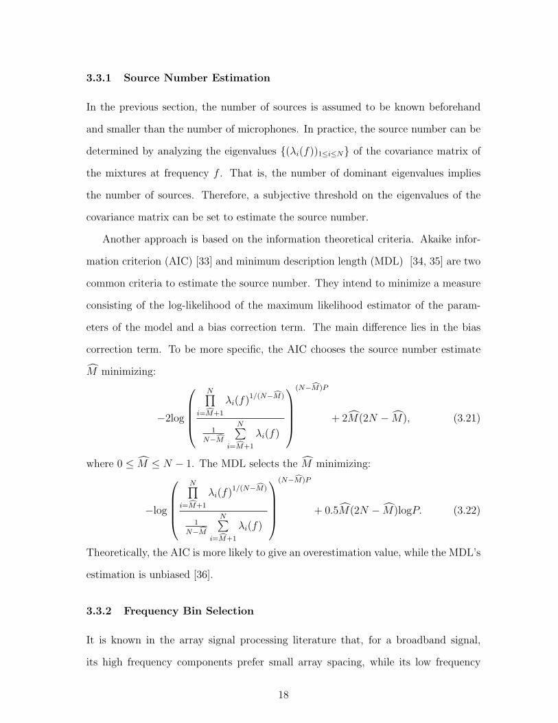
Another approach is based on the information theoretical criteria. Akaike infor-

mation criterion (AIC) [33] and minimum description length (MDL) [34, 35] are two

common criteria to estimate the source number. They intend to minimize a measure

consisting of the log-likelihood of the maximum likelihood estimator of the param-

eters of the model and a bias correction term. The main difference lies in the bias

correction term. To be more specific, the AIC chooses the source number estimate

M minimizing:

−2log

N∏i=M+1

λi(f)1/(N−M)

1

N−M

N∑i=M+1

λi(f)

(N−M)P

+ 2M(2N − M), (3.21)

where 0 ≤ M ≤ N − 1. The MDL selects the M minimizing:

−log

N∏i=M+1

λi(f)1/(N−M)

1

N−M

N∑i=M+1

λi(f)

(N−M)P

+ 0.5M(2N − M)logP. (3.22)

Theoretically, the AIC is more likely to give an overestimation value, while the MDL’s

estimation is unbiased [36].

3.3.2 Frequency Bin Selection

It is known in the array signal processing literature that, for a broadband signal,

its high frequency components prefer small array spacing, while its low frequency

18

parts prefer large spacing. In reality, a given microphone array is fixed and signals of

interest can be different. In [37], the authors propose using microphones with different

spacing to handle different frequency ranges respectively. That is, considering that

we need multiple microphones to perform localization, we may select only a subset

of the microphones to perform the localization for lower frequency signals, as long

as the source number is less than the number of chosen microphones. Therefore, a

microphone array can handle a wider range of signals.

0 1000 2000 3000 4000 5000 6000 7000 8000

−80

−60

−40

−20

0

20

40

60

80

Frequency (Hz)

Est

imat

ed D

OA

(de

gree

)

Estimated DOA vs frequency at SNR = 20 dB

Source at −40 degreeSource at 40 degree

Figure 3.2: DOA estimate versus frequency for two sources at -40 and 40 degrees.

0 1000 2000 3000 4000 5000 6000 7000 8000

−80

−60

−40

−20

0

20

40

60

80

Frequency (Hz)

Est

imat

ed D

OA

(de

gree

)

Estimated DOA vs frequency at SNR = 20 dB

Source at −80 degreeSource at 40 degree

Figure 3.3: DOA estimate versus frequency for two sources at -80 and 40 degrees.

19

A microphone array samples signals in the space domain. Similar to the aliasing

problem for sampling in the time domain, a microphone array also experiences a

spatial aliasing problem. In the time domain, the well-known Nyquist sampling theory

tells that to recover a signal with the highest frequency fmax, the sampling rate

is at least 2fmax. In the spatial sampling, it requires that half of the minimum

wavelength of a wideband signal should be larger than the interval of the array upon

which it impinges. To be more specific, for a microphone spacing d, the maximum

frequency it can capture accurately is c/(2d), where c is the velocity of sound in

the medium. In our problem, the phase delay between two microphones should be

smaller than π in modulus, i.e., |2πfdsin(θ)/c| ≤ π. For example, when d = 0.05

m, c = 340 m/s, θ1 = −40 degree, and θ2 = 40 degree, the spatial aliasing occurs

at c/2/sin(40π/180) = 5289.5Hz. Figure 3.2 shows how the estimated DOA changes

with frequency. At around 5000 Hz, the DOA estimate becomes drastically inaccurate.

When θ1 = −80 degree, θ2 = 40 degree, and other parameters remain the same, the

spatial aliasing occurs at c/(2sin(80π/180)) = 3452.5 Hz. Figure 3.3 shows that the

tipping point where the estimate becomes much worse is at around 3400 Hz. This

suggests that we only focus on the frequency range where no spatial aliasing occurs.

On the other hand, if the frequency of a signal is too low and thus its wavelength

is too long, the array can only capture a very tiny amount of the phase change of the

signal. From Figures 3.2 and 3.3, it is clear that the DOA estimate is significantly

worse at low frequencies than at higher frequencies. Therefore, a lower frequency

threshold is also set. Although audio signals are naturally broadband, we can only

consider some specific frequencies, at which the algorithm can estimate the DOAs

more accurately.

20

0 2000 4000 6000 8000 10000 12000 14000 160000

5

10

15

20

25

30

35

40

Frequency (Hz)

Val

ue

Norm of the first row of the demixing matrix vs frequency

Figure 3.4: Norm of the first row of W(f) versus frequency f .

3.3.3 Artifact Filtering

It is noted that for estimated DOAs, mixing matrix A(f)’s columns are linearly

dependent at certain harmonic frequencies so that W(f) becomes extremely large at

these frequencies. For example, Figure 3.4 shows one example of how the second norm

of the first row of the estimated demixing matrix W(f) changes with frequency using

the estimated DOAs. It is clear that the large values are distributed at harmonic

frequencies. Consequently, recovered signals include burbling artifacts, which are

known as “musical notes” in the literature [38]. An easy way to eliminate these

artifacts is to use certain filters to eliminate the recovered signals at these frequencies.

3.3.4 Different Ways of Mixture Generation

The subspace methods utilize the phase differences among the mixtures collected by

different microphones. Namely, the success of our algorithm largely depends on the

accuracy of the phase difference measurements among array signals. In practice, we

21

only have discrete time signals and correspondingly measured time delays are only

approximated by an integer number of sampling intervals. Therefore, sampling rate

plays an important role. For our algorithm to work, it should satisfy the condition:

dsinθ/c ≥ 1

Fs

. (3.23)

For small angles and low sampling rates, the algorithm may fail if time domain mix-

tures are used, due to the fact that the delay may be less than a sampling interval

and there will be no delay and phase change information in the collected mixtures

at different microphones. In other words, sampling results in rounding errors in the

measured phase changes and time delays, and generating biases in the DOA esti-

mates. The round error in the time delay between two adjacent microphones equals

(dsinθ/c− NFs) second(s), where N = floor(dsinθFs/c), and floor(a) returns the nearest

integer no larger than a.

In simulations, we try two different mixing approaches to reduce or eliminate the

effect of sampling. First is to use source signals with as high sample rates as possible.

Second is to use mixtures in the frequency domain so that the phase information

is free from the sampling effect. That is, the mixture is generated by the formula

X(p, f) = A(f)S(p, f) + N(p, f), and the SNRs are set in the time domain. For

frequency domain mixtures, the phase differences among different microphones are

totally preserved. While this may not reflect the natural experimental procedure,

this helps us focus on other aspects of the algorithm without the finite sampling rate

effect. Figure 3.5 shows the difference in obtaining a time domain mixture and a

frequency domain mixture.

3.3.5 Relation with Beamforming and Spatial Filtering

We use the subspace methods to estimate the DOAs of sources and separate the source

signals using the DOA estimates. This is essentially related to spatial filtering, or

beamforming in the array signal processing literature. It shows that in the simulations

22

A(f)

Frequency domain mixture

Time domain mixture

Figure 3.5: Two different kinds of mixtures.

and experiments, even if the estimated DOAs which are deviated significantly from

the true ones are used, and thus the separation performance becomes worse and

burbling artifacts are significant, the original sounds can still be audible clearly from

the recovered files. Especially, when the sources are widely separated, as long as the

estimates can roughly reflect the spatial locations of the sources, the sounds can be

heard without too much performance loss.

3.3.6 Performance Measures

The performance measures used for evaluation include the mean squared error (MSE)

of DOA or coordinate estimates for localization and the signal-to-distortion ratio

(SDR), the signal-to-interferences ratio (SIR), and the signal-to-artifacts ratio (SAR)

for separation, which are firstly introduced in [38]. The MSE of DOA estimate θm(f)

for source m at frequency f is computed as

MSEθm(f) =

∑i

(θm,i(f)− θm)2

I, (3.24)

where I is the number of Monte Carlo runs. The MSE of DOA estimate θm is

computed as

MSEθm =

∑i

(θm,i − θm)2

I, (3.25)

The MSE of source coordinate estimate vm for source m is computed as

MSEvm=

∑i

||vm,i − vm||2

I. (3.26)

23

where vm and vm,i are D×1 vectors, and D is the dimension of the coordinate system.

In our problem, we consider the two-dimension system, i.e., D = 2.

For separation, it is assumed that the recovered source signal can be decomposed

through orthogonal projections as

sm = starget + einterf + enoise + eartif, (3.27)

where starget is a modified version of sm with an allowed distortion, einterf, enoise, and

eartif are respectively the interferences, noise, and artifacts terms. sm, starget, einterf,

enoise, and eartif are L × 1 vectors, and L is the source signal length measured in

samples.

To be more specific, let∏{z1, z2, · · · , zj} represent the orthogonal projector onto

the subspace spanned by the vectors z1, z2, · · · , zj . The projector is a J × J matrix,

where J is the length of these vectors. The decomposition includes three projectors:

Psm :=∏

{sm}, (3.28)

Ps :=∏

{(sm)1≤m≤M}, (3.29)

and

Ps,n :=∏

{(sm)1≤m≤M , (nn)1≤n≤N}. (3.30)

where sm and nm are L× 1 vectors. The four terms are written as follows:

starget := Psm sm, (3.31)

sinterf := Pssm − Psm sm, (3.32)

snoise := Ps,nsm − Pssm, (3.33)

24

and

sartif := sm − Ps,nsm. (3.34)

The SDR is defined as

SDR = 10 log10||starget||2

||einterf + enoise + eartif||2. (3.35)

The SIR is defined as

SIR = 10 log10||starget||2||einterf||2

. (3.36)

The SAR is defined as

SAR = 10 log10||starget + einterf + enoise||2

||eartif||2. (3.37)

The underlying assumption is that the ground truth source signals and noise are

known. The existing computer algorithms for recovered signal decomposition and

SDR, SAR, and SIR computation can be found in [39].

3.3.7 Source Coordinate Estimation using Multiple Arrays

Figure 3.6: Relative delay mixing.

One array can estimate the DOAs of sources, and multiple arrays can together

determine the coordinates of the sources. Once we have the DOA estimates for the

same source at multiple arrays, its coordinates can be computed using triangulation

techniques combined with the knowledge about the coordinates of the arrays. In our

localization scheme, we assume that different sources have different source angles with

respect to one array. The underlying assumption here is that the sources are placed

25

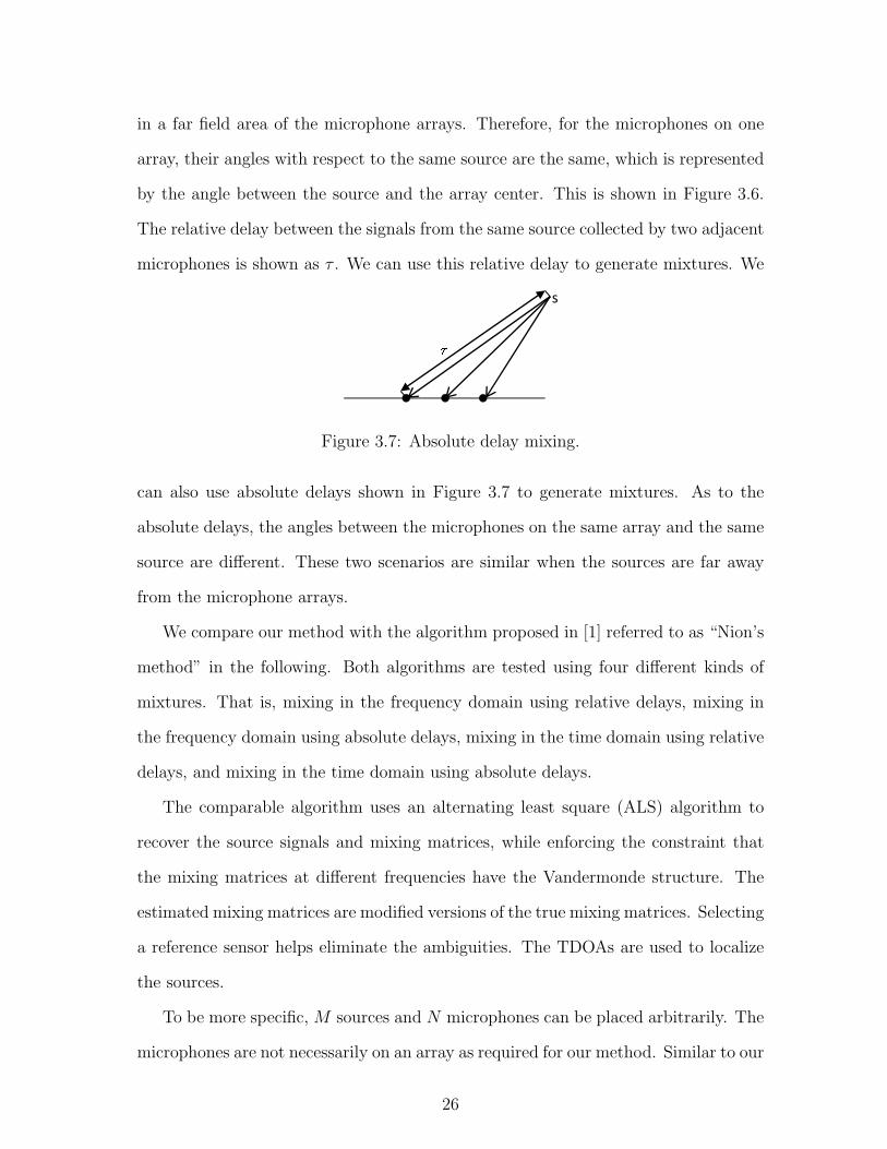
in a far field area of the microphone arrays. Therefore, for the microphones on one

array, their angles with respect to the same source are the same, which is represented

by the angle between the source and the array center. This is shown in Figure 3.6.

The relative delay between the signals from the same source collected by two adjacent

microphones is shown as τ . We can use this relative delay to generate mixtures. We

s

Figure 3.7: Absolute delay mixing.

can also use absolute delays shown in Figure 3.7 to generate mixtures. As to the

absolute delays, the angles between the microphones on the same array and the same

source are different. These two scenarios are similar when the sources are far away

from the microphone arrays.

We compare our method with the algorithm proposed in [1] referred to as “Nion’s

method” in the following. Both algorithms are tested using four different kinds of

mixtures. That is, mixing in the frequency domain using relative delays, mixing in

the frequency domain using absolute delays, mixing in the time domain using relative

delays, and mixing in the time domain using absolute delays.

The comparable algorithm uses an alternating least square (ALS) algorithm to

recover the source signals and mixing matrices, while enforcing the constraint that

the mixing matrices at different frequencies have the Vandermonde structure. The

estimated mixing matrices are modified versions of the true mixing matrices. Selecting

a reference sensor helps eliminate the ambiguities. The TDOAs are used to localize

the sources.

To be more specific, M sources and N microphones can be placed arbitrarily. The

microphones are not necessarily on an array as required for our method. Similar to our

26

formulation, the received mixture at microphone n is represented in Equation (3.1).

Moreover, it is not necessarily a far field, and the DOAs of the same source are not

necessarily equal for the multiple microphones on the same array.

After performing K point STFT,

Xn(p, fk) =M∑

m=1

anmSm(p, fk)e−j2πfkτnm +Nn(p, fk), (3.38)

where fk = Fs(k − 1)/K represents the frequency value, for k = 1, · · · , F , and

F = floor(K/2) + 1. f is the shorthand notation for fk in the following. The noise

part is ignored in the theoretical analysis for the sake of simplicity. Therefore,

X(f) = H(f)S(f), (3.39)

where [X(f)]n,p = Xn(p, f), [S(f)]m,p = Sm(p, f), w = e−j2π, and [H(f)]m,n =

anmwfτnm .

Define Hn,m,f = [H(f)]n,m, hnm = Hn,m,1:F = [anmwf1τnm , · · · , anmwfF τnm ]T has a

Vandermonde structure. Namely, hnm = anm[b0, b1, · · · , bF ]T , where b = wτnmFs/K .

Then, X ∈ CF×N×P and Sn ∈ CF×F×P , which are defined by Xf,n,p = Xn(p, f) and

[Sm]:,:,p = diag([Sm(p, 1), Sm(p, 2), · · · , Sm(p, F )]), respectively. Let Hm ∈ CF×N be

the channel Vandermonde matrix for source m, which is defined as [Hm]:,n = hnm,

where Hm is the part of H related to source m. Therefore,

X =M∑

m=1

Sm •2 HTm. (3.40)

where •2 is the tensor product operator. Figure 3.8 shows the tensor representation

of Equation (3.40). Based on the received data X(fk), for k = 1, · · · , F , the ALS

algorithm with the Vandermonde structure enforcement on hnm is implemented to

recover the H(f) and S(f) alternatively at each frequency. Due to the ambiguities

inherent in the algorithm, it only recovers a modified version of H(f). That is,

hnm = [anmwf1τnm , · · · , anmwfF τnm ]. Therefore, a reference microphone mR is chosen

to eliminate the ambiguities and the TDOAs are obtained: τnm = τnm − τnmR=

27

Figure 3.8: The tensor representation of the problem [1].

τnm − τnmR. After having the multiple TDOAs, the sources are localized by solving a

constrained optimization problem. A drawback of Nion’s method is that it does not

guarantee to converge. Its separation and localization results heavily depend on the

initialization step. It is also time consuming.

28

CHAPTER 4

SIMULATIONS AND EXPERIMENTS FOR OUTDOOR

ENVIRONMENTS

In this section, we firstly use MATLAB simulations to show the performance of the

proposed algorithm. Then, we use experiments to show its effectiveness in real world

environments. We mainly use uniform linear arrays and the ESPRIT method, given

that the ESPRIT can directly give DOA estimates.

4.1 Simulations

4.1.1 Simulation Setup

In the simulations, there are N = 4 microphones uniformly and linearly distributed

with spacing d = 0.05 m. M = 2 sources are located at directions θ1 = 40 and

θ2 = −40 degrees, respectively. Source signals include music and speeches. They are

normalized into signals with zero mean and unit variance. The velocity of sound in

the air is c = 340 m/s. The sampling rate is 16 kHz. The noise is set to be zero mean

additive white Gaussian noise (AWGN) with variance σ2 across microphones. It is

noted that for audio signals, the power at different frequencies are different, while

the power of white noise at different frequencies are ideally equal. The signal-to-noise

ratio is set to be 10log10(M/σ2). We only consider the frequency range without spatial

aliasing. That is, in our simulations, f ≤ c/(2d). We use 10000 Monte Carlo runs for

each SNR. Additionally, in all simulations, due to the inability of a microphone array

to capture low frequency signals, we set a lower frequency threshold to be 1 kHz. The

parameter setting in simulations is summarized in Table 4.1.

29

Table 4.1: Parameter setting in simulations.

Mixture characteristics Parameters to be specified

Number of sources M 2

Source categories Speech & music

Source length 4 seconds

Source angles +/- 40◦

Noise type AWGN (sensor noise)

Number of microphones N 4

Array spacing d 0.05 m

Sampling rate Fs 16 kHz

Mixture type Pure delay mixture

Mixture domain Frequency domain

Frame length 256

Frame shift 256

FFT window Rectangular

Chosen frequency percentage 30%

Monte Carlo runs 10000

4.1.2 Source Spectrogram

The diverse time-frequency characteristics of audio signals can be illustrated by their

spectrograms, which are the signal amplitude values as a function of time-frequency.

Figure 4.1 shows the spectrograms of four sources. Source1 and Source2 are male and

female speeches, respectively. Source3 and Source4 correspond to trumpet and piano

music. They show typical time-frequency characteristics for each category. That

is, speeches generally cross a wide spectrum and short time duration, while music

consists of harmonic frequencies and is more continuous in time.

30

(a) Source1 (Male speech) (b) Source2 (Female speech)

(c) Source3 (Trumpet music) (d) Source4 (Piano music)

Figure 4.1: The spectrograms of different sources.

31

1000 1500 2000 2500 3000−70

−60

−50

−40

−30

−20

−10

0

Eigenvalues vs frequency with SNR = 30 dB

Frequency (Hz)

Eig

enva

lues

(dB

)

(a) Mixture of Source1 and Source3

1000 1500 2000 2500 3000−70

−60

−50

−40

−30

−20

−10

0


Frequency (Hz)

Eig

enva

lues

(dB

)

(b) Mixture of Source2 and Source4

Figure 4.2: Normalized eigenvalues versus frequency for different source combinations

with SNR = 30 dB.


Eigenvalue based Method

Figure 4.2 shows the normalized eigenvalues of the covariance matrix at different

frequencies for different source combinations at SNR = 30 dB. The plots are obtained

by averaging the results over total 10000 runs. It is clear that for different sources,

the whole trend of how eigenvalues change with frequency is different. With SNR =

30 dB, the first two eigenvalues are much larger than the rest eigenvalues for most of

the frequencies. It is relatively easy to set a subjective threshold to decide the source

number. That is, when the signal power is dominant in the mixture, using eigenvalue

analysis to estimate source number is suitable.

Figure 4.3 shows the results for SNR = 10 dB. It is shown that for the mixture

of Soure1 and Source3, at almost all frequencies, the two largest eigenvalues are

significantly larger than the remaining two smaller eigenvalues. Therefore, the number

of sources can be estimated accurately. For the mixture of Source2 and Source4, at

frequencies from 1000 Hz to around 2000 Hz, the two largest eigenvalues can be

32

1000 1500 2000 2500 3000−70

−60

−50

−40

−30

−20

−10

0


Frequency (Hz)

Eig

enva

lues

(dB

)

(a) Mixture of Source1 and Source3

1000 1500 2000 2500 3000−70

−60

−50

−40

−30

−20

−10

0


Frequency (Hz)

Eig

enva

lues

(dB

)

(b) Mixture of Source2 and Source4

Figure 4.3: Normalized eigenvalues versus frequency for different source combinations

with SNR = 10 dB.

easily distinguished from the rest. The two smaller eigenvalues are very close to

the second largest eigenvalues at higher frequencies, which introduces ambiguities

in the estimation of the source number. Intuitively, at lower SNRs, it will become

more difficult to estimate the number of sources accurately by setting a threshold.

Moreover, from Figure 4.3, we can learn that the differences in the patterns of how the

eigenvalues change with frequency are closely related to the characteristics of sources.

Information Theoretical Criteria

Information theoretical criteria include Akaike information criterion (AIC) and min-

imum description length (MDL). Figures 4.4 and 4.5 show the percentage of correct

source number estimates in total 10000 runs using AIC and MDL at SNR = 30 dB

and 10 dB, respectively.

They indicate that higher SNRs bring a better source number estimation perfor-

mance. At low SNRs, like 10 dB, source number estimation can be very different at

different frequencies because of the difference of power distribution across frequency.

For example, in Figures 4.5(c) and 4.5(d), the source number estimation accuracy at

33

1000 1500 2000 2500 30000

0.2

0.4

0.6

0.8

1

AIC based estimate vs frequency at SNR = 30 dB

Frequency (Hz)

Cor

rect

est

imat

ion

perc

enta

ge (

%)

(a) Mixture of Source1 and Source3 using AIC

1000 1500 2000 2500 30000

0.2

0.4

0.6

0.8

1

MDL based estimate vs frequency at SNR = 30 dB

Frequency (Hz)

Cor

rect

est

imat

ion

perc

enta

ge (

%)

(b) Mixture of Source1 and Source3 using MDL

1000 1500 2000 2500 30000

0.2

0.4

0.6

0.8

1


Frequency (Hz)

Cor

rect

est

imat

ion

perc

enta

ge (

%)

(c) Mixture of Source2 and Source4 using AIC

1000 1500 2000 2500 30000

0.2

0.4

0.6

0.8

1


Frequency (Hz)

Cor

rect

est

imat

ion

perc

enta

ge (

%)

(d) Mixture of Source2 and Source4 using MDL

Figure 4.4: Correct estimation percentage versus frequency for different source com-

binations with SNR = 30 dB using AIC and MDL.

34

1000 1500 2000 2500 30000

0.2

0.4

0.6

0.8

1


Frequency (Hz)

Cor

rect

est

imat

ion

perc

enta

ge (

%)

(a) Mixture of Source1 and Source3 using AIC

1000 1500 2000 2500 30000

0.2

0.4

0.6

0.8

1


Frequency (Hz)

Cor

rect

est

imat

ion

perc

enta

ge (

%)

(b) Mixture of Source1 and Source3 using MDL

1000 1500 2000 2500 30000

0.2

0.4

0.6

0.8

1


Frequency (Hz)

Cor

rect

est

imat

ion

perc

enta

ge (

%)

(c) Mixture of Source2 and Source4 using AIC

1000 1500 2000 2500 30000

0.2

0.4

0.6

0.8

1


Frequency (Hz)

Cor

rect

est

imat

ion

perc

enta

ge (

%)

(d) Mixture of Source2 and Source4 using MDL

Figure 4.5: Correct estimation percentage versus frequency for different source com-

binations with SNR = 10 dB using AIC and MDL.

35

1000 1500 2000 2500 3000−4

−2

0

2

4MSE vs frequency

Frequency (Hz)

MS

E (

log1

0 sc

ale)

source1(−40)source3(40)

(a) -10 dB

1000 1500 2000 2500 3000−4

−2

0

2

4MSE vs frequency

Frequency (Hz)

MS

E (

log1

0 sc

ale)


(b) -5 dB

1000 1500 2000 2500 3000−4

−2

0

2

4MSE vs frequency

Frequency (Hz)

MS

E (

log1

0 sc

ale)


(c) 0 dB

1000 1500 2000 2500 3000−4

−2

0

2

4MSE vs frequency

Frequency (Hz)

MS

E (

log1

0 sc

ale)


(d) 5dB

1000 1500 2000 2500 3000−4

−2

0

2

4MSE vs frequency

Frequency (Hz)

MS

E (

log1

0 sc

ale)


(e) 10 dB

1000 1500 2000 2500 3000−4

−2

0

2

4MSE vs frequency

Frequency (Hz)

MS

E (

log1

0 sc

ale)


(f) 15 dB

1000 1500 2000 2500 3000−4

−2

0

2

4MSE vs frequency

Frequency (Hz)

MS

E (

log1

0 sc

ale)


(g) 20 dB

1000 1500 2000 2500 3000−4

−2

0

2

4MSE vs frequency

Frequency (Hz)

MS

E (

log1

0 sc

ale)


(h) 25 dB

1000 1500 2000 2500 3000−4

−2

0

2

4MSE vs frequency

Frequency (Hz)

MS

E (

log1

0 sc

ale)


(i) 30 dB

Figure 4.6: MSE versus frequency at different SNRs using Source1 and Source3.

certain frequencies larger than 2000 Hz deteriorates a lot. This is because there is

much less power distributed above 2 kHz for Source2 and Source4, compared to the

power distributed below 2 kHz, which is obvious from their spectrograms. There-

fore, for an accurate source number estimation, it’s desirable to have some knowledge

about how the power of source signals is distributed across frequency.

36

1000 1500 2000 2500 3000−4

−2

0

2

4MSE vs frequency

Frequency (Hz)

MS

E (

log1

0 sc

ale)


(a) -10 dB

1000 1500 2000 2500 3000−4

−2

0

2

4MSE vs frequency

Frequency (Hz)

MS

E (

log1

0 sc

ale)


(b) -5 dB

1000 1500 2000 2500 3000−4

−2

0

2

4MSE vs frequency

Frequency (Hz)

MS

E (

log1

0 sc

ale)


(c) 0 dB

1000 1500 2000 2500 3000−4

−2

0

2

4MSE vs frequency

Frequency (Hz)

MS

E (

log1

0 sc

ale)


(d) 5 dB

1000 1500 2000 2500 3000−4

−2

0

2

4MSE vs frequency

Frequency (Hz)

MS

E (

log1

0 sc

ale)


(e) 10 dB

1000 1500 2000 2500 3000−4

−2

0

2

4MSE vs frequency

Frequency (Hz)

MS

E (

log1

0 sc

ale)


(f) 15 dB

1000 1500 2000 2500 3000−4

−2

0

2

4MSE vs frequency

Frequency (Hz)

MS

E (

log1

0 sc

ale)


(g) 20 dB

1000 1500 2000 2500 3000−4

−2

0

2

4MSE vs frequency

Frequency (Hz)

MS

E (

log1

0 sc

ale)


(h) 25 dB

1000 1500 2000 2500 3000−4

−2

0

2

4MSE vs frequency

Frequency (Hz)

MS

E (

log1

0 sc

ale)


(i) 30 dB

Figure 4.7: MSE versus frequency at different SNRs using Source2 and Source4.

37

4.1.4 θm(f) Estimation and Associated Separation

θm(f) Estimation Performance

Figures 4.6 and 4.7 show the MSE versus frequency at different SNRs using the

mixture of Source1 and Source3, and using the mixture of Source2 and Source4,

respectively. It is obvious that with higher SNRs, the MSE performance is much

better. For different source files, the patterns of MSE versus frequency curves are

very different. This is likely to be related to the SNR difference of different signals at

different frequencies and at different time locations. In other words, it is because of

the differences of different source files in time-frequency characteristics.

Separation Performance

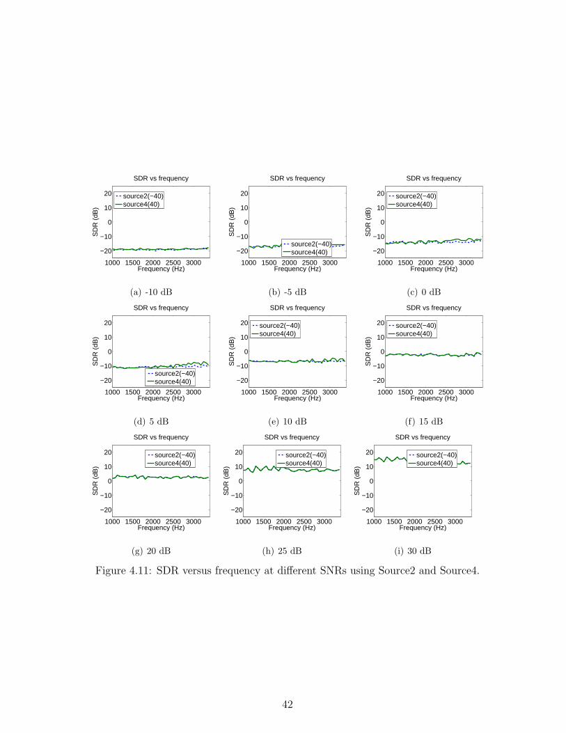
Figures 4.8, 4.9, 4.10, 4.11, 4.12, and 4.13 show the average SDR, SAR, and SIR versus

frequency at different SNRs for different source combinations. Similarly, higher SNRs

bring a better separation performance. Among these three measures, the SDR is most

frequently used, due to the fact that it is the ratio of the power of the desired part of

a recovered signal to the power of the undesired part.

It shows that at low SNRs, the SDR, SAR, and SIR values are extremely small,

which indicates inaccurate DOA estimates and correspondingly an enormous amount

of noise, artifacts, and interferences. As the SNR increases, the DOA estimates

become more accurate, and thus the separation performance is better. Moreover, the

SDR and SAR curves become more similar as the SNR increases. This is because the

noise term diminishes with a higher SNR. At the same time, due to the improvement

in the DOA estimates, the interference term also diminishes. In the simulations, the

sources are widely separated. As the SNR increases to as low as 0dB, the SAR has

been around 5 dB. The SAR and SIR have already become similar, which means that

the interference term has become significantly small. Therefore, the SDR and SAR

38

1000 1500 2000 2500 3000

−20

−10

0

10

20

Frequency (Hz)

SD

R (

dB)

SDR vs frequency


(a) -10 dB

1000 1500 2000 2500 3000

−20

−10

0

10

20

Frequency (Hz)

SD

R (

dB)

SDR vs frequency


(b) -5 dB

1000 1500 2000 2500 3000

−20

−10

0

10

20

Frequency (Hz)

SD

R (

dB)

SDR vs frequency


(c) 0 dB

1000 1500 2000 2500 3000

−20

−10

0

10

20

Frequency (Hz)

SD

R (

dB)

SDR vs frequency


(d) 5 dB

1000 1500 2000 2500 3000

−20

−10

0

10

20

Frequency (Hz)

SD

R (

dB)

SDR vs frequency


(e) 10 dB

1000 1500 2000 2500 3000

−20

−10

0

10

20

Frequency (Hz)

SD

R (

dB)

SDR vs frequency


(f) 15 dB

1000 1500 2000 2500 3000

−20

−10

0

10

20

Frequency (Hz)

SD

R (

dB)

SDR vs frequency


(g) 20 dB

1000 1500 2000 2500 3000

−20

−10

0

10

20

Frequency (Hz)

SD

R (

dB)

SDR vs frequency


(h) 25 dB

1000 1500 2000 2500 3000

−20

−10

0

10

20

Frequency (Hz)

SD

R (

dB)

SDR vs frequency


(i) 30 dB

Figure 4.8: SDR versus frequency at different SNRs using Source1 and Source3.

39

1000 1500 2000 2500 3000

−20

−10

0

10

20

SAR vs frequency

Frequency (Hz)

SA

R (

dB)


(a) -10 dB

1000 1500 2000 2500 3000

−20

−10

0

10

20

SAR vs frequency

Frequency (Hz)

SA

R (

dB)


(b) -5 dB

1000 1500 2000 2500 3000

−20

−10

0

10

20

SAR vs frequency

Frequency (Hz)

SA

R (

dB)


(c) 0 dB

1000 1500 2000 2500 3000

−20

−10

0

10

20

SAR vs frequency

Frequency (Hz)

SA

R (

dB)


(d) 5 dB

1000 1500 2000 2500 3000

−20

−10

0

10

20

SAR vs frequency

Frequency (Hz)

SA

R (

dB)


(e) 10 dB

1000 1500 2000 2500 3000

−20

−10

0

10

20

SAR vs frequency

Frequency (Hz)

SA

R (

dB)


(f) 15 dB

1000 1500 2000 2500 3000

−20

−10

0

10

20

SAR vs frequency

Frequency (Hz)

SA

R (

dB)


(g) 20 dB

1000 1500 2000 2500 3000

−20

−10

0

10

20

SAR vs frequency

Frequency (Hz)

SA

R (

dB)


(h) 25 dB

1000 1500 2000 2500 3000

−20

−10

0

10

20

SAR vs frequency

Frequency (Hz)

SA

R (

dB)


(i) 30 dB

Figure 4.9: SAR versus frequency at different SNRs using Source1 and Source3.

40

1000 1500 2000 2500 3000

0

10

20

30

40

Frequency (Hz)

SIR

(dB

)

SIR vs frequency


(a) -10 dB

1000 1500 2000 2500 3000

0

10

20

30

40

Frequency (Hz)

SIR

(dB

)

SIR vs frequency


(b) -5 dB

1000 1500 2000 2500 3000

0

10

20

30

40

Frequency (Hz)

SIR

(dB

)

SIR vs frequency


(c) 0 dB

1000 1500 2000 2500 3000

0

10

20

30

40

Frequency (Hz)

SIR

(dB

)

SIR vs frequency


(d) 5 dB

1000 1500 2000 2500 3000

0

10

20

30

40

Frequency (Hz)

SIR

(dB

)

SIR vs frequency


(e) 10 dB

1000 1500 2000 2500 3000

0

10

20

30

40

Frequency (Hz)

SIR

(dB

)

SIR vs frequency


(f) 15 dB

1000 1500 2000 2500 3000

0

10

20

30

40

Frequency (Hz)

SIR

(dB

)

SIR vs frequency


(g) 20 dB

1000 1500 2000 2500 3000

0

10

20

30

40

Frequency (Hz)

SIR

(dB

)

SIR vs frequency


(h) 25 dB

1000 1500 2000 2500 3000

0

10

20

30

40

Frequency (Hz)

SIR

(dB

)

SIR vs frequency


(i) 30 dB

Figure 4.10: SIR versus frequency at different SNRs using Source1 and Source3.

41

1000 1500 2000 2500 3000

−20

−10

0

10

20

Frequency (Hz)

SD

R (

dB)

SDR vs frequency


(a) -10 dB

1000 1500 2000 2500 3000

−20

−10

0

10

20

Frequency (Hz)

SD

R (

dB)

SDR vs frequency


(b) -5 dB

1000 1500 2000 2500 3000

−20

−10

0

10

20

Frequency (Hz)

SD

R (

dB)

SDR vs frequency


(c) 0 dB

1000 1500 2000 2500 3000

−20

−10

0

10

20

Frequency (Hz)

SD

R (

dB)

SDR vs frequency


(d) 5 dB

1000 1500 2000 2500 3000

−20

−10

0

10

20

Frequency (Hz)

SD

R (

dB)

SDR vs frequency


(e) 10 dB

1000 1500 2000 2500 3000

−20

−10

0

10

20

Frequency (Hz)

SD

R (

dB)

SDR vs frequency


(f) 15 dB

1000 1500 2000 2500 3000

−20

−10

0

10

20

Frequency (Hz)

SD

R (

dB)

SDR vs frequency


(g) 20 dB

1000 1500 2000 2500 3000

−20

−10

0

10

20

Frequency (Hz)

SD

R (

dB)

SDR vs frequency


(h) 25 dB

1000 1500 2000 2500 3000

−20

−10

0

10

20

Frequency (Hz)

SD

R (

dB)

SDR vs frequency


(i) 30 dB

Figure 4.11: SDR versus frequency at different SNRs using Source2 and Source4.

42

1000 1500 2000 2500 3000

−20

−10

0

10

20

SAR vs frequency

Frequency (Hz)

SA

R (

dB)


(a) -10 dB

1000 1500 2000 2500 3000

−20

−10

0

10

20

SAR vs frequency

Frequency (Hz)

SA

R (

dB)


(b) -5 dB

1000 1500 2000 2500 3000

−20

−10

0

10

20

SAR vs frequency

Frequency (Hz)

SA

R (

dB)


(c) 0 dB

1000 1500 2000 2500 3000

−20

−10

0

10

20

SAR vs frequency

Frequency (Hz)

SA

R (

dB)


(d) 5 dB

1000 1500 2000 2500 3000

−20

−10

0

10

20

SAR vs frequency

Frequency (Hz)

SA

R (

dB)


(e) 10 dB

1000 1500 2000 2500 3000

−20

−10

0

10

20

SAR vs frequency

Frequency (Hz)

SA

R (

dB)


(f) 15 dB

1000 1500 2000 2500 3000

−20

−10

0

10

20

SAR vs frequency

Frequency (Hz)

SA

R (

dB)


(g) 20 dB

1000 1500 2000 2500 3000

−20

−10

0

10

20

SAR vs frequency

Frequency (Hz)

SA

R (

dB)


(h) 25 dB

1000 1500 2000 2500 3000

−20

−10

0

10

20

SAR vs frequency

Frequency (Hz)

SA

R (

dB)


(i) 30 dB

Figure 4.12: SAR versus frequency at different SNRs using Source2 and Source4.

43

1000 1500 2000 2500 3000

0

10

20

30

40

Frequency (Hz)

SIR

(dB

)

SIR vs frequency


(a) -10 dB

1000 1500 2000 2500 3000

0

10

20

30

40

Frequency (Hz)

SIR

(dB

)

SIR vs frequency


(b) -5 dB

1000 1500 2000 2500 3000

0

10

20

30

40

Frequency (Hz)

SIR

(dB

)

SIR vs frequency


(c) 0 dB

1000 1500 2000 2500 3000

0

10

20

30

40

Frequency (Hz)

SIR

(dB

)

SIR vs frequency


(d) 5 dB

1000 1500 2000 2500 3000

0

10

20

30

40

Frequency (Hz)

SIR

(dB

)

SIR vs frequency


(e) 10 dB

1000 1500 2000 2500 3000

0

10

20

30

40

Frequency (Hz)

SIR

(dB

)

SIR vs frequency


(f) 15 dB

1000 1500 2000 2500 3000

0

10

20

30

40

Frequency (Hz)

SIR

(dB

)

SIR vs frequency


(g) 20 dB

1000 1500 2000 2500 3000

0

10

20

30

40

Frequency (Hz)

SIR

(dB

)

SIR vs frequency


(h) 25 dB

1000 1500 2000 2500 3000

0

10

20

30

40

Frequency (Hz)

SIR

(dB

)

SIR vs frequency


(i) 30 dB

Figure 4.13: SIR versus frequency at different SNRs using Source2 and Source4.

44

−10 0 10 20 30−4

−3

−2

−1

0

1

2

3

4MSE vs SNR

SNR (dB)

MS

E (

log1

0 sc

ale)


(a) Mixtures of Source1 and Source3

−10 0 10 20 30−4

−3

−2

−1

0

1

2

3

4MSE vs SNR

SNR (dB)

MS

E (

log1

0 sc

ale)


(b) Mixtures of Source2 and Source4

Figure 4.14: MSE versus SNR using the average of DOA estimates for different source

combinations.

formulas become quite close to each other. As the SNR becomes about 30 dB, the

SIR is extremely large, and the SAR and SIR are extremely similar. All of these

observations corroborate the idea of beamforming or spatial filtering.

4.1.5 θm Estimation and Associated Separation

θm Estimation Performance

Figures 4.14 and 4.15 show the MSE of DOA estimates versus SNR using the average

and weighted average. Basically, these two methods have similar localization perfor-

mance. It is obvious that for different source combinations and two different DOA

determination methods, better localization is achieved with increasing SNRs.

Separation Performance

Figures 4.16 and 4.18 show how the SDR, SIR, and SAR change with SNR using

the average and weighted average for mixture of Source1 and Source3. Figures 4.17

and 4.19 show the results for mixture of Source2 and Source4. Similar to the local-

45

−10 0 10 20 30−4

−3

−2

−1

0

1

2

3

4MSE vs SNR

SNR (dB)

MS

E (

log1

0 sc

ale)


(a) Mixtures of Source1 and Source3

−10 0 10 20 30−4

−3

−2

−1

0

1

2

3

4MSE vs SNR

SNR (dB)

MS

E (

log1

0 sc

ale)


(b) Mixtures of Source2 and Source4

Figure 4.15: MSE versus SNR using the weighted average of DOA estimates for

different source combinations.

−10 0 10 20 30

−20

−10

0

10

20

SNR (dB)

SD

R (

dB)

SDR vs SNR


(a) SDR vs SNR

−10 0 10 20 30

−20

−10

0

10

20

SAR vs SNR

SNR (dB)

SA

R (

dB)


(b) SAR vs SNR

−10 0 10 20 30

−20

−10

0

10

20

SIR vs SNR

SNR (dB)

SIR

(dB

)


(c) SIR vs SNR

Figure 4.16: SDR, SAR, and SIR versus SNR using the average of DOA estimates

for mixture of Source1 and Source3.

−10 0 10 20 30

−20

−10

0

10

20

SNR (dB)

SD

R (

dB)

SDR vs SNR


(a) SDR vs SNR

−10 0 10 20 30

−20

−10

0

10

20

SAR vs SNR

SNR (dB)

SA

R (

dB)


(b) SAR vs SNR

−10 0 10 20 30

−20

−10

0

10

20

SIR vs SNR

SNR (dB)

SIR

(dB

)


(c) SIR vs SNR

Figure 4.17: SDR, SAR, and SIR versus SNR using the average of DOA estimates

for mixture of Source2 and Source4.

46

−10 0 10 20 30

−20

−10

0

10

20

SNR (dB)

SD

R (

dB)

SDR vs SNR


(a) SDR vs SNR

−10 0 10 20 30

−20

−10

0

10

20

SAR vs SNR

SNR (dB)

SA

R (

dB)


(b) SAR vs SNR

−10 0 10 20 30

−20

−10

0

10

20

SIR vs SNR

SNR (dB)

SIR

(dB

)


(c) SIR vs SNR

Figure 4.18: SDR, SAR, and SIR versus SNR using the weighted average of DOA

estimates for mixture of Source1 and Source3.

−10 0 10 20 30

−20

−10

0

10

20

SNR (dB)

SD

R (

dB)

SDR vs SNR


(a) SDR vs SNR

−10 0 10 20 30

−20

−10

0

10

20

SAR vs SNR

SNR (dB)

SA

R (

dB)


(b) SAR vs SNR

−10 0 10 20 30

−20

−10

0

10

20

SIR vs SNR

SNR (dB)

SIR

(dB

)


(c) SIR vs SNR

Figure 4.19: SDR, SAR, and SIR versus SNR using the weighted average of DOA

estimates for mixture of Source2 and Source4.

47

Table 4.2: Parameter setting for comparison.

Parameters Values

Number of arrays U 2


Number of microphone on each array R 5

Time duration 4 seconds

Inter-microphone spacing d 0.05 m

Velocity of sound c 340 m/s

Frame length 1024

Frame shift 1024

Sampling rate Fs 16 kHz

Window function Rectangular or Hanning window

Lower frequency threshold 1 kHz

Chosen frequency percentage 30%

ization performance, the separation performance improves with increasing SNRs, due

to more accurate DOA estimates.

4.1.6 Source Coordinate Estimation and Separation using Multiple Ar-

rays

We compare our method with Nion’s method in two ways. One is to use the same array

configuration for these two methods. The other is to use the array configuration for

our algorithm and an arbitrary configuration for Nion’s method. Table 4.2 summarizes

the parameter setting for comparison.

48

Table 4.3: Comparison with Nion’s method.

Our method Nion’s method

Localization DOA TDOA

Microphone placement Array Arbitrary

Attenuation coefficients Uniform (far field) Arbitrary

Real-time implementation√ ×

Absolute time mixture√

separation (√) & localization (×)

Absolute frequency mixture√


Relative time mixture√


Relative frequency mixture√


With the Same Array Configuration for the two methods

Figure 4.20 shows the spatial configuration of microphone arrays and sources. Ta-

ble 4.3 gives the comparison of our method and Nion’s method.

0 0.5 1 1.5 2 2.5 30

0.5

1

1.5

2

2.5

3

s1

s2

x coordinate (in meter)

y co

ordi

nate

(in

met

er)

spatial configuration

Figure 4.20: Spatial configuration for algorithm comparison.

Nion’s method works in separation and fails in localization for all four kinds of

mixtures. The reason may be the relatively special locations of the microphones. To

49

−10 0 10 20 30−1

0

1

2

3

4

5

SNR (dB)

MS

E (

log1

0 sc

ale)

MSE vs SNR using the same configuration for comparison

Our MethodNion’s Method

Figure 4.21: MSE vs SNR using two methods for the same configuration.

be more specific, the microphones are on parallel linear arrays. Moreover, the spacing

is small and so are the corresponding delays. The microphone signals on the same

array experience the spatial aliasing.

For our algorithm, if time domain mixtures are used, the performance of the

algorithm using a Hanning window is much better than the performance when using

a rectangular window. A rectangular window has a high peak side lobe value, which

means that the ringing effect is significant, and a wide main lobe, indicating its large

smoothing effect. On the other hand, a Hanning window has a relatively narrower

main lobe and a lower peak side lobe value. Therefore, its smoothing effect and

ringing effect are both less significant than a rectangular window. All of these are

related to the spectral leakage of a finite discrete Fourier transform (DFT) window.

By using absolute delay mixtures in the time domain, we compare the separation

and localization performance of these two methods. Figure 4.21 shows the MSE

of source coordinate estimates at different SNRs. Our algorithm generally has a

decreasing MSE as the SNR increases. However, Nion’s method gives a constant

MSE. It should be emphasized that the MSE performance of these two methods at

50

−10 0 10 20 30−25

−20

−15

−10

−5

0

SNR (dB)

SD

R (

dB)

Average SDR vs SNR


(a) SDR vs SNR

−10 0 10 20 30−20

−15

−10

−5

0

5

SNR (dB)

SA

R (

dB)

Average SAR vs SNR


(b) SAR vs SNR

−10 0 10 20 300

5

10

15

20

SNR (dB)

SIR

(dB

)

Average SIR vs SNR


(c) SIR vs SNR

Figure 4.22: SDR, SAR, SIR versus SNR using two methods for the same configura-

tion.

0 0.5 1 1.5 2 2.5 30

0.5

1

1.5

2

2.5

3

m1

m2 m3

m4

m5

m6

m7

m8

m9

m10

s1

s2

x coordinate (in meter)

y co

ordi

nate

(in

met

er)

spatial configuration

Figure 4.23: Spatial configuration for Nion’s method.

low SNRs is extremely bad.

Figure 4.22 shows how the SDR, SAR, and SIR change with SNR using these

two methods. It is clear that two algorithms are close in the separation performance.

Specifically, at lower SNRs, our algorithm is a little better in all SDR, SAR, and SIR,

while Nion’s method becomes better in SDR, SAR, and SIR at higher SNRs. As to

why the SIR for our algorithm becomes worse for large SNRs, it is subject to a further

exploration.

51

−10 0 10 20 30−2

−1

0

1

2

3

4

5

SNR (dB)

MS

E (

log1

0 sc

ale)

MSE vs SNR using different configurations for comparison


Figure 4.24: MSE vs SNR using two methods for different configurations.

−10 0 10 20 30−25

−20

−15

−10

−5

0

SNR (dB)

SD

R (

dB)

Average SDR vs SNR


(a) SDR vs SNR

−10 0 10 20 30−20

−15

−10

−5

0

5

SNR (dB)

SA

R (

dB)

Average SAR vs SNR


(b) SAR vs SNR

−10 0 10 20 300

5

10

15

20

SNR (dB)

SIR

(dB

)

Average SIR vs SNR


(c) SIR vs SNR

Figure 4.25: SDR, SAR, SIR versus SNR using two methods for different configura-

tions.

52

With Different Configurations for the two methods

Our algorithm still uses the same configuration as shown in Figure 4.20, while for

Nion’s method, an arbitrary microphone placement as shown in Figure 4.23 is used.

That is, 10 microphones are randomly placed in a 3× 3 area. Figure 4.24 shows the

MSE comparison results of source coordinate estimation. Nion’s method performs

better than ours in source localization. When the microphones are arbitrarily placed,

the relative delays among different source and microphone pairs tend to become large.

Therefore, the rounding error due to the sampling rate is relatively smaller and its

effect becomes less significant. Therefore, the localization performance of Nion’s

method using an arbitrary microphone placement becomes better. In other words,

although the two MSE curves become flat after certain points, the MSE of Nion’s

method achieves a lower level due to smaller biases in the relative delays.

Figure 4.25 shows the SDR, SAR, and SIR values using these two methods at dif-

ferent SNRs. It shows that the separation performance of our algorithm is generally

better than Nion’s method. Basically, the separation and localization performance of

Nion’s method isn’t as closely related to each other as our method. Using the array

configuration, Nion’s method fails in the localization, while is still able to separate the

sources and its performance is close to ours. However, when it has a better localiza-

tion performance than ours using an arbitrary microphone placement, its localization

performance is still inferior to ours most of the time.

4.2 Outdoor Experiments

This section uses real world experiments to test various aspects of our algorithm for

outdoor environments.

53

Figure 4.26: An NI cDAQ 9171 USB chassis and four microphones.

4.2.1 Experimental Description

We perform the experiments in an open area between two buildings. A rectangular

wooden frame is used to support four microphones forming an array. We use an NI

cDAQ 9171 USB chassis, shown in Figure 4.26, to connect four microphones with a

laptop. The microphones are omnidirectional and the highest sampling rate is 51.2

kHz. Two USB-powered loud speakers are placed at the same side of the microphone

array as the audio sources. After collecting certain length of signals, our algorithm

is used to estimate the DOAs of the sources. Figure 4.27 illustrates one example

of the experiment setup. The main noise source in outdoor environments is wind,

which significantly affects the performance of our algorithm. The parameter setting

for experiments is summarized in Table 4.4.


Information Theoretical Criteria for Source Number Estimation

Figures 4.28 shows the percentage of correct estimate using AIC and MDL criteria. It

is clear that, contrary to the results in simulations, the performance in the experiments

is much worse. It might be attributed to two factors. One is the SNR. In real

54

Figure 4.27: An example of the experimental setup.

1000 1500 2000 2500 30000

0.2

0.4

0.6

0.8

1

AIC based estimate vs frequency

Frequency (Hz)

Per

cent

age

(%)

(a) AIC

1000 1500 2000 2500 30000

0.2

0.4

0.6

0.8

1

MDL based estimate vs frequency

Frequency (Hz)

Cor

rect

est

imat

ion

Per

cent

age

(%)

(b) MDL

Figure 4.28: Correct source number estimation percentage versus frequency using

AIC and MDL.

55

Table 4.4: Parameter setting for outdoor experiments.

Experimental Parameters Values


Source categories Speech & music

Source length 4 seconds

Number of microphones N 4

Array spacing d 0.05 m

Sampling rate Fs 51.2 kHz

Frame length 1024

Frame shift 1024

FFT window Rectangular

experiments, the SNRs are unknown and may be quite small. The other is the noise

type, which is likely to have more significant influence. The assumption for these

two criteria is that the noise is Gaussian in the time domain or circular complex

Gaussian in the frequency domain. This may not be the case in real environments,

which explains why the methods fail to estimate the source number correctly most of

the time.

Eigenvalue Based Source Number Estimation

Figure 4.29 shows the average normalized eigenvalues of the spatial covariance matrix

of the collected mixtures. In total, 491 experiment files are used. It is clear that the

eigenvalues for signals and noise are well separated, especially at high frequencies. If

we have some prior knowledge about the background noise, it is easy to estimate the

number of the sources accurately.

56

1000 1500 2000 2500 3000

−30

−20

−10

0

Normalized eigenvalues vs frequency

Frequency (Hz)

Nor

mal

ized

eig

enva

lues

(dB

)

Figure 4.29: Average normalized eigenvalues versus frequency using experimental

files.

Figure 4.30: The spectrogram of the background noise.

57

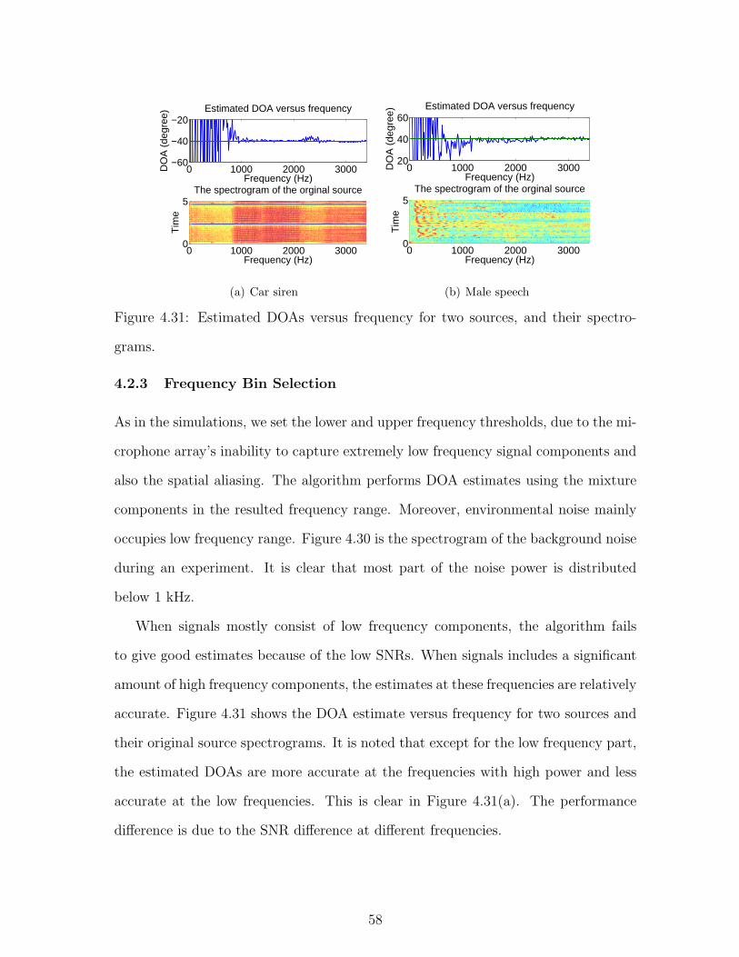
0 1000 2000 3000−60

−40

−20

Frequency (Hz)

DO

A (

degr

ee) Estimated DOA versus frequency

0 1000 2000 30000

5

Frequency (Hz)

The spectrogram of the orginal source

Tim

e

(a) Car siren

0 1000 2000 300020

40

60

Frequency (Hz)

DO

A (

degr

ee) Estimated DOA versus frequency

0 1000 2000 30000

5

Frequency (Hz)

The spectrogram of the orginal source

Tim

e

(b) Male speech

Figure 4.31: Estimated DOAs versus frequency for two sources, and their spectro-

grams.

4.2.3 Frequency Bin Selection

As in the simulations, we set the lower and upper frequency thresholds, due to the mi-

crophone array’s inability to capture extremely low frequency signal components and

also the spatial aliasing. The algorithm performs DOA estimates using the mixture

components in the resulted frequency range. Moreover, environmental noise mainly

occupies low frequency range. Figure 4.30 is the spectrogram of the background noise

during an experiment. It is clear that most part of the noise power is distributed

below 1 kHz.

When signals mostly consist of low frequency components, the algorithm fails

to give good estimates because of the low SNRs. When signals includes a significant

amount of high frequency components, the estimates at these frequencies are relatively

accurate. Figure 4.31 shows the DOA estimate versus frequency for two sources and

their original source spectrograms. It is noted that except for the low frequency part,

the estimated DOAs are more accurate at the frequencies with high power and less

accurate at the low frequencies. This is clear in Figure 4.31(a). The performance

difference is due to the SNR difference at different frequencies.

58

CHAPTER 5

CONCLUSIONS AND FUTURE WORK

5.1 Conclusions

A subspace-based audio signal separation and localization scheme has been proposed

for pure delay mixtures collected by microphone arrays. The algorithm applies the

STFT to the mixtures and uses the subspace methods, such as MUSIC and ESPRIT,

to estimate the DOAs of audio sources at each frequency independently. The DOA

estimates at frequencies with large SSA values are combined to obtain the final DOA

estimates. Correspondingly, the mixing and demixing matrices are computed, and

the source signals are recovered using the inverse STFT.

The algorithm is robust to noise at the cost of more microphones than sources.

Also, the permutation issue does not exist for our algorithm. Our localization-based

separation approach is essentially a beamformer, which extracts the signals at es-

timated DOAs from collected mixtures. Moreover, it supports real-time implemen-

tation. That is, the required signal length is generally short. Unlike optimization-

based source separation methods, it directly gives the DOA estimates and in turn the

demixing matrices, and does not resort to iterative computations. We have discussed

several crucial issues closely related to the algorithm and their solutions, including

source number estimation, spatial aliasing, different ways of mixture generation, fre-

quency bin selection, and artifact filtering. Both simulations and experiments have

been conducted to test the effectiveness and performance of the algorithm.

59

5.2 Future Work

In the future, we intend to consider the sound localization and separation problem

in more challenging and realistic indoor reverberant environments as well as the un-

derdetermined and critically determined scenarios. We will also try to develop new

methods applicable for real world experiments, while taking the current state-of-the-

art methods into consideration.

60

BIBLIOGRAPHY

[1] D. Nion, B. Vandewoestyne, S. Vanaverbeke, K. Van Den Abeele, H. De Gersem,

and L. De Lathauwer, A Time-Frequency Technique for Blind Separation and

Localization of Pure Delayed Sources Latent Variable Analysis and Signal Sepa-

ration, vol. 6365 of Lecture Notes in Computer Science, pp. 546–554. Springer

Berlin / Heidelberg, 2010.

[2] S. Makeig, A. J. Bell, T. ping Jung, and T. J. Sejnowski, “Independent compo-

nent analysis of electroencephalographic data,” in in Advances in Neural Infor-

mation Processing Systems, pp. 145–151, MIT Press, 1996.

[3] E. C. Cherry, “Some experiments on the recognition of speech, with one and

with two ears,” Journal of the Acoustical Society of America, vol. 25, no. 5, p. 5,

1953.

[4] K. Kokkinakis and P. C. Loizou, “Using blind source separation techniques to

improve speech recognition in bilateral cochlear implant patients,” Journal of

the Acoustical Society of America, vol. 123, no. 4, p. 12, 2008.

[5] M. Sahiduilah and G. Saha, “Design, analysis and experimental evaluation of

block based transformation in mfcc computation for speaker recognition,” Speech

Communication, vol. 54, no. 4, pp. 543–565, 2012.

[6] M. D. Plumbley, S. A. Abdallah, J. P. Bello, M. E. Davies, G. Monti, and M. B.

Sandler, “Automatic music transcription and audio source separation,” 2001.

[7] M. Brandstein and D. E. Ward, Microphone arrays: signal processing techniques

and applications. Springer-Verlag Berlin, 2001.

61

[8] J. Dmochowski, J. Benesty, and S. Affes, “On spatial aliasing in microphone

arrays,” Signal Processing, IEEE Transactions on, vol. 57, no. 4, pp. 1383–1395,

2009.

[9] V. C. Chen and L. Hao, “Joint time-frequency analysis for radar signal and image

processing,” Signal Processing Magazine, IEEE, vol. 16, no. 2, pp. 81–93, 1999.

[10] A. Hyvarinen and E. Oja, “Independent component analysis: algorithms and

applications,” Neural Netw., vol. 13, no. 4-5, pp. 411–430, 2000.

[11] O. Yilmaz and S. Rickard, “Blind separation of speech mixtures via time-

frequency masking,” Signal Processing, IEEE Transactions on, vol. 52, no. 7,

pp. 1830–1847, 2004.

[12] D. Wang and G. J. Brown, Computational Auditory Scene Analysis: Principles,

Algorithms, and Applications. Hoboken, NJ: Wiley, 2006.

[13] M. I. Mandel, R. J. Weiss, and D. Ellis, “Model-based expectation-maximization

source separation and localization,” Audio, Speech, and Language Processing,

IEEE Transactions on, vol. 18, no. 2, pp. 382–394, 2010.

[14] A. J. Bell and T. J. Sejnowski, “An information-maximization approach to blind

separation and blind deconvolution,” Neural Computation, vol. 7, pp. 1129–1159,

1995.

[15] P. Smaragdis, “Blind separation of convolved mixtures in the frequency domain,”

February 9-10 1998.

[16] H. Sawada, S. Araki, and S. Makino, “Measuring dependence of bin-wise sep-

arated signals for permutation alignment in frequency-domain bss,” in Circuits

and Systems, 2007. ISCAS 2007. IEEE International Symposium on, pp. 3247–

3250, 2007.

62

[17] H. Sawada, R. Mukai, S. Araki, and S. Makino, “A robust and precise method for

solving the permutation problem of frequency-domain blind source separation,”

Speech and Audio Processing, IEEE Transactions on, vol. 12, no. 5, pp. 530–538,

2004.

[18] H. Sawada, S. Araki, and S. Makino, “Underdetermined convolutive blind source

separation via frequency bin-wise clustering and permutation alignment,” Audio,

Speech, and Language Processing, IEEE Transactions on, vol. 19, no. 3, pp. 516–

527, 2011.

[19] H. Sawada, R. Mukai, and S. Makino, “Direction of arrival estimation for multiple

source signals using independent component analysis,” in Signal Processing and

Its Applications, 2003. Proceedings. Seventh International Symposium on, vol. 2,

pp. 411–414 vol.2, 2003.

[20] S. Kurita, H. Saruwatari, S. Kajita, K. Takeda, and F. Itakura, “Evaluation

of blind signal separation method using directivity pattern under reverberant

conditions,” in Acoustics, Speech, and Signal Processing, 2000. ICASSP ’00.

Proceedings. 2000 IEEE International Conference on, vol. 5, pp. 3140–3143 vol.5,

2010.

[21] Y. Li, S.-I. Amari, A. Cichocki, D. Ho, and S. Xie, “Underdetermined blind

source separation based on sparse representation,” IEEE Transactions on Signal

Processing, vol. 54, no. 2, pp. 423 – 437, 2006.

[22] E. Vincent, S. Araki, F. Theis, G. Nolte, P. Bofill, H. Sawada, A. Ozerov,

V. Gowreesunker, D. Lutter, and N. Q. K. Duong, “The signal separation eval-

uation campaign (20072010): Achievements and remaining challenges,” Signal

Processing, vol. 92, no. 8, pp. 1928–1936, 2012.

63

[23] A. Ozerov and C. Fevotte, “Multichannel nonnegative matrix factorization in

convolutive mixtures for audio source separation,” Audio, Speech, and Language

Processing, IEEE Transactions on, vol. 18, no. 3, pp. 550–563, 2010.

[24] P. Aarabi, “Self-localizing dynamic microphone arrays,” Systems, Man, and Cy-

bernetics, Part C: Applications and Reviews, IEEE Transactions on, vol. 32,

no. 4, pp. 474–484, 2002.

[25] Z. Wenyi and B. D. Rao, “A two microphone-based approach for source localiza-

tion of multiple speech sources,” Audio, Speech, and Language Processing, IEEE

Transactions on, vol. 18, no. 8, pp. 1913–1928, 2010.

[26] R. Schmidt, “Multiple emitter location and signal parameter estimation,” An-

tennas and Propagation, IEEE Transactions on, vol. 34, no. 3, pp. 276–280,

1986.

[27] R. Roy and T. Kailath, “Esprit-estimation of signal parameters via rotational

invariance techniques,” Acoustics, Speech and Signal Processing, IEEE Transac-

tions on, vol. 37, no. 7, pp. 984–995, 1989.

[28] H. Buchner, R. Aichner, and W. Kellermann, TRINICON-based Blind System

Identification with Application to Multiple-Source Localization and Separation

Blind Speech Separation, pp. 101–147. Signals and Communication Technology,

Springer Netherlands, 2007.

[29] T. May, S. van de Par, and A. Kohlrausch, “A binaural scene analyzer for joint

localization and recognition of speakers in the presence of interfering noise sources

and reverberation,” Audio, Speech, and Language Processing, IEEE Transactions

on, vol. 20, no. 7, pp. 2016–2030, 2012.

64

[30] T. May, S. van de Par, and A. Kohlrausch, “A probabilistic model for robust lo-

calization based on a binaural auditory front-end,” Audio, Speech, and Language

Processing, IEEE Transactions on, vol. 19, no. 1, pp. 1–13, 2011.

[31] F. Asano, S. Hayamizu, T. Yamada, and S. Nakamura, “Speech enhancement

based on the subspace method,” Speech and Audio Processing, IEEE Transac-

tions on, vol. 8, no. 5, pp. 497–507, 2000.

[32] P. Stoica and T. Soderstrom, “Statistical analysis of music and subspace rotation

estimates of sinusoidal frequencies,” Trans. Sig. Proc., vol. 39, no. 8, pp. 1836–

1847, 1991.

[33] H. Akaike, “A new look at the statistical model identification,” Automatic Con-

trol, IEEE Transactions on, vol. 19, no. 6, pp. 716–723, 1974.

[34] J. Rissanen, “Modeling by shortest data description,” Automatica, vol. 14, no. 5,

pp. 465–471, 1978.

[35] G. Schwarz, “Estimating the dimension of a model,” Annals of Statistics, vol. 6,

p. 4, 1978.

[36] M. Wax and T. Kailath, “Detection of signals by information theoretic criteria,”

Acoustics, Speech and Signal Processing, IEEE Transactions on, vol. 33, no. 2,

pp. 387–392, 1985.

[37] S. Winter, H. Sawada, and S. Makino, “Geometrical interpretation of the pca

subspace approach for overdetermined blind source separation,” EURASIP J.

Appl. Signal Process., vol. 2006, pp. 176–176, 2006.

[38] E. Vincent, R. Gribonval, and C. Fevotte, “Performance measurement in blind

audio source separation,” Audio, Speech, and Language Processing, IEEE Trans-

actions on, vol. 14, no. 4, pp. 1462–1469, 2006.

65

[39] C. Fevotte, R. Gribonval, and E. Vincent, “Bss eval toolbox user guide.” http:

//www.irisa.fr.metiss/bss\_eval, 2005.

[40] H. Wang and M. Kaveh, “Coherent signal-subspace processing for the detection

and estimation of angles of arrival of multiple wide-band sources,” Acoustics,

Speech and Signal Processing, IEEE Transactions on, vol. 33, no. 4, pp. 823–

831, 1985.

[41] L. Chang; and C.-F. Twu;, “The estimation of direction-of-arrival of wideband

sources by signal subspace focusing approach,” Journal of Marine Science and

Technology, vol. 6, no. 1, pp. 9–15, 1998.

[42] Y.-S. Yoon, Direction-of-arrival estimation of wideband sources using sensor ar-

rays. PhD thesis, 2004.

66

VITA

Longji Sun

Candidate for the Degree of

Master of Science

Thesis: BLIND SOURCE SEPARATION AND LOCALIZATION USING MICRO-PHONE ARRAYS

Major Field: Electrical Engineering

Biographical:

Personal Data: Born in Dengzhou, Henan, China, on December 3rd, 1988.

Education:Received the Bachelor of Engineering (B.E.) degree from University ofShanghai for Science and Technology, Shanghai, China, 2010, in Commu-nication EngineeringCompleted the requirements for the degree of Master of Science (M.S.)with a major in Electrical Engineering from Oklahoma State University inDecember, 2012.

Experience:Research assistant, School of Electrical and Computer Engineering, Okla-homa State University, 08/2010-present

Professional Memberships:Institute of Electrical and Electronics Engineers (IEEE)The Honor Society of Phi Kappa Phi

Name: Longji Sun Date of Degree: December, 2012

Institution: Oklahoma State University Location: Stillwater, Oklahoma

Title of Study: BLIND SOURCE SEPARATION AND LOCALIZATION USINGMICROPHONE ARRAYS

Pages in Study: 66 Candidate for the Degree of Master of Science

Major Field: Electrical Engineering

The blind source separation and localization problem for audio signals is studiedusing microphone arrays. Pure delay mixtures of source signals typically encounteredin outdoor environments are considered. Our proposed approach utilizes the subspacemethods, including multiple signal classification (MUSIC) and estimation of signalparameters via rotational invariance techniques (ESPRIT) algorithms, to estimatethe directions of arrival (DOAs) of the sources from the collected mixtures. Sinceaudio signals are generally considered broadband, the DOA estimates at frequencieswith the large sum of squared amplitude values are combined to obtain the finalDOA estimates. Using the estimated DOAs, the corresponding mixing and demixingmatrices are computed, and the source signals are recovered using the inverse shorttime Fourier transform.

Subspace methods take advantage of the spatial covariance matrix of the collectedmixtures to achieve robustness to noise. While the subspace methods have been stud-ied for localizing radio frequency signals, audio signals have their special properties.For instance, they are nonstationary, naturally broadband and analog. All of thesemake the separation and localization for the audio signals more challenging. More-over, our algorithm is essentially equivalent to the beamforming technique, whichsuppresses the signals in unwanted directions and only recovers the signals in theestimated DOAs.

Several crucial issues related to our algorithm and their solutions have been discussed,including source number estimation, spatial aliasing, artifact filtering, different waysof mixture generation, and source coordinate estimation using multiple arrays. Addi-tionally, comprehensive simulations and experiments have been conducted to examinevarious aspects of the algorithm. Unlike the existing blind source separation and lo-calization methods, which are generally time consuming, our algorithm needs signalmixtures of only a short duration and therefore supports real-time implementation.

ADVISOR’S APPROVAL: Dr. Qi Cheng

blind source separation and localization using … · blind source separation (bss) recovers...

Documents