BLAZE: Blazing Fast Privacy-Preserving MachineLearning

Arpita Patra∗, Ajith Suresh∗∗Department of Computer Science and Automation, Indian Institute of Science, Bangalore India

{arpita, ajith}@iisc.ac.in

Abstract—Machine learning tools have illustrated their poten-tial in many significant sectors such as healthcare and finance, toaide in deriving useful inferences. The sensitive and confidentialnature of the data, in such sectors, raise natural concernsfor the privacy of data. This motivated the area of Privacy-preserving Machine Learning (PPML) where privacy of the datais guaranteed. Typically, ML techniques require large computingpower, which leads clients with limited infrastructure to rely onthe method of Secure Outsourced Computation (SOC). In SOCsetting, the computation is outsourced to a set of specialized andpowerful cloud servers and the service is availed on a pay-per-use basis. In this work, we explore PPML techniques in theSOC setting for widely used ML algorithms– Linear Regression,Logistic Regression, and Neural Networks.

We propose BLAZE, a blazing fast PPML framework in thethree server setting tolerating one malicious corruption over aring (Z2` ). BLAZE achieves the stronger security guarantee offairness (all honest servers get the output whenever the corruptserver obtains the same). Leveraging an input-independent pre-processing phase, BLAZE has a fast input-dependent online phaserelying on efficient PPML primitives such as: (i) A dot productprotocol for which the communication in the online phase isindependent of the vector size, the first of its kind in the threeserver setting; (ii) A method for truncation that shuns evaluatingexpensive circuit for Ripple Carry Adders (RCA) and achievesa constant round complexity. This improves over the truncationmethod of ABY3 (Mohassel et al., CCS 2018) that uses RCA andconsumes a round complexity that is of the order of the depthof RCA (which is same as the underlying ring size).

An extensive benchmarking of BLAZE for the aforementionedML algorithms over a 64-bit ring in both WAN and LANsettings shows massive improvements over ABY3. Concretely,we observe improvements up to 333× for Linear Regression,53× for Logistic Regression and 276× for Neural Networksover WAN. Similarly, we show improvements up to 2610× forLinear Regression, 54× for Logistic Regression and 278× forNeural Networks over LAN.

I. INTRODUCTION

Machine learning (ML) is increasingly becoming one ofthe dominant research fields. Advancement in the domain hasmyriad real-life applications– from smart keyboard predictionsto more involved operations such as self-driving cars. It alsofinds useful applications in impactful fields such as healthcareand medicine, where ML tools are being used to assist health-care specialists in better diagnosing abnormalities. This surgein interest in the field is bolstered by the availability of a largeamount of data with the rise of companies such as Googleand Amazon. This is also due to improved, more robust andaccurate ML algorithms in use today. With better machineryand tools such as deep learning and reinforcement learning,

ML techniques are starting to beat humans at some difficulttasks such as classifying echocardiograms [1].

In order to be deployed in practice, ML models facenumerous challenges. The primary challenge is to providea high level of accuracy and robustness, as it is imperativefor the functioning of some mission-critical fields such ashealth care. Accuracy and robustness are contingent on a highamount of computing power and availability of data from morevaried sources. Accumulating data from different and varioussources is not practical for a single company/stake-holder torealize. Moreover, policies like the European Union GeneralData Protection Regulation (GDPR) or the EFF’s call forinformation fiduciary rules for businesses have made it difficultand even illegal for companies to share datasets with each otherwithout the prior consent of customers. In some cases, it mighteven be infeasible for companies to share their data with eachother as it is proprietary information and sharing it may giverise to concerns such as competitive advantage. While in othercases, the data might be too sensitive, such as medical andfinancial records, that a breach of privacy cannot be tolerated.It is also possible that the companies providing ML servicesto clients risk leaking the model parameters rendering itsservices redundant, and the individual client’s or company’sdata no longer private. In the light of huge interest in usingML and simultaneous requirement of security of data, the fieldof privacy-preserving machine learning (PPML) has emergedas a flourishing research area. These techniques can be used toensure that no information about the query or dataset is leakedother than what is permissible by the algorithm, which in somecases might be only the prediction output.

The primary challenge that inhibits widespread adoptionof PPML is that the additional demand on privacy makesthe already compute-intensive ML algorithms all the moredemanding not just in terms of high compute power but alsoin terms of other complexity measures such as communica-tion complexity that the privacy-preserving techniques entail.Many everyday end-users are not equipped with computinginfrastructure capable of efficiently executing these algorithms.It is economical and convenient for end-users to outsource anML task to more powerful and specialized systems. However,even while outsourcing to servers, the privacy of data mustbe ensured. Towards this, we use Secure Outsourced Compu-tation (SOC) as a potential solution. SOC allows end-usersto securely outsource computation to a set of specialized andpowerful cloud servers and avail its services on a pay-per-use basis. SOC guarantees that individual data of the end-users remain private, tolerating reasonable collusion amongstthe servers.

PPML, both for training and inference, can be realizedin the SOC setting. Firstly, an end-user posing as a model-owner can host its trained machine learning model, in a secret-shared way, to a set of (untrusted) servers. An end-user as acustomer can secret-share its query amongst the same serversto allow the prediction to be computed in a shared fashion andto finally obtain the prediction result. Secondly, multiple data-owners can host their datasets in a shared way amongst a setof (untrusted) servers and can train a common model on theirjoint datasets while keeping their individual dataset private.Recently, many works [2]–[6], solve the aforementioned goalsusing the techniques of Secure Multiparty Computation (MPC)where the untrusted servers are taken as the participants (orparties) of the MPC. The corrupt server(s) can collude withan arbitrary number of data-owners in case of training and witheither the model-owner or the customer in case of inference.Privacy of the end-users is ensured leveraging the securityguarantees of MPC.

MPC is arguably the standard-bearer problem in cryp-tography. It allows n mutually distrusting parties to performcomputations together on their private inputs, so that anadversary controlling at most t parties, can not learn anyinformation beyond what is already known and permissibleby the computation. MPC for a small number of parties in thehonest majority setting, specifically the setting of 3 parties withone corruption, has become popular over the last few years dueto its spectacular performance [7]–[17], leveraging the pres-ence of single corruption. Applications such as financial dataanalysis [18], email spam filtering [19], distributed credentialencryption [12], privacy-preserving statistical studies [20] andpopular MPC frameworks such as Sharemind [21], VIFF [22]involve 3 parties.

In an effort to improve the practical efficiency, manyrecent works divide their protocol into two phases, namely– i)input-independent preprocessing phase and ii) input-dependentonline phase. This has become a prominent approach in boththeoretical [23]–[28] and practical [4], [29]–[36] domains. Thepreprocessing phase is used to perform a relatively expensivecomputation that is independent of the input. In the onlinephase, once the inputs become available, the actual compu-tation can be performed in a fast way making use of thepre-computed data. This paradigm suits scenarios analogousto our setting, where functions typically need to be evaluateda large number of times, and the function description is knownbeforehand.

There has been a recent paradigm shift of designing MPCover rings, considering the fact that computer architecturesuse rings of size 32 or 64 bits. Designing and implementingMPC protocols over rings can leverage CPU optimizations andhave been proven to have a significant impact on efficiency[21], [34], [37]–[39]. Furthermore, operating over rings avoidsthe need to overload basic operations such as addition andmultiplication during implementation, or rely on an externallibrary as compared to working over prime order fields.

Although MPC techniques can be used to realize SOC,the current best MPC techniques cannot be directly pluggedinto ML algorithms, largely due to the following reasons.Firstly, in ML domain, most of the computation happens overdecimal values, requiring us to embed the decimal valuesin 2’s complement form over a ring (Z2` ), where the MSB

represents the sign bit, followed by a designated number of bitsrepresenting the integer part and fractional part. As a naturalconsequence of this embedding, repeated multiplications causean overflow in the ring, with the fractional part doubling upin size after each multiplication and occupying double thenumber of its original bit assignment. The naive solution isto pick a ring large enough to avoid the overflow, but thenumber of sequential multiplications in a typical ML algorithmmakes this solution impractical. The existing works [2], [5],[6] tackled this problem through a secure truncation, a veryimportant primitive by now, which approximates the value bysacrificing the accuracy by an infinitesimal amount, performedafter every multiplication. Essentially, the truncation applied ina privacy-preserving way gets the result of the multiplicationback to the same format as that of the inputs, by right-shiftingit and thereby slashing the expansion of the fractional partcaused by the multiplication. Secondly, certain functions suchas comparison or the widely used activation such as ReLU orSigmoid, requiring extraction of MSB in a privacy-preservingmanner, needs involvement of the boolean world (over the ringZ21 ), while functions such as addition, dot product are moreefficient when performed in the arithmetic domain (over thering Z2` ). The ML algorithms involve a mix of operations,constantly alternating between these two worlds. As shownin some of the recent works [2], [5], [38], using mixed worldcomputation is orders of magnitude more efficient as comparedto most of the current best MPC techniques which operate onlyin either of the two worlds. Thirdly, while a typical MPC offersa way to tackle a multiplication gate, ML algorithms invoke itsvariant dot product. A naive way of doing privacy-preservingdot product would invoke the method of multiplication ` times,with ` being the size of the input vectors. With ML algorithmsdealing with humongous size data vectors, the naive approachmay turn expensive and so customized way of performingdot product that attains independence from the vector sizein its complexity is called for. In other words, PPML wouldneed customized privacy-preserving building blocks, such asdot product, truncation, comparison, ReLU, Sigmoid etc.,rather than the typical building blocks such as addition andmultiplication of MPC.

A. Related Work

In the regime of PPML using MPC, earlier works consid-ered the widely-used ML algorithms such as Decision Trees[40], Linear Regression [41], [42], k-means clustering [43],[44], SVM Classification [45], [46], and Logistic Regression[47]. However, these solutions are far from practical due tothe high overheads that they incur. SecureML [2] proposeda practically-efficient PPML framework in the two-servermodel using a mix of 2PC protocols that perform computationin Arithmetic, Boolean and Yao style (aka. ABY frame-work [38]). One of their key contributions is a novel method fortruncating decimal numbers. They consider training for linearregression, logistic regression, and neural network models. Thework of Chameleon [4] considered a 2PC setting where partiesavailed the help of a semi-trusted third party and considerSVMs and Neural Networks. Both SecureML and Chameleonconsidered semi-honest corruption only. The ABY frameworkwas extended to the three-party setting by ABY3 [5] andSecureNN [6] (the latter consider neural networks only). Theseworks consider malicious security and demonstrate that the

2

honest-majority setting can be leveraged to improve the perfor-mance by several orders of magnitude. Recently, ASTRA [48]furthered this line of work and improve upon ABY3. However,ASTRA presents a set of primitives to build protocols forLinear Regression and Logistic Regression inference. For thetraining of these ML algorithms and NN prediction, additionalprimitives like truncation, bit to arithmetic conversions arerequired, which are not considered in ASTRA.

B. Our Contribution

We propose an efficient PPML framework over the ring Z2`

in a SOC setting, with three servers amongst which at most onecan be maliciously corrupt. The framework consists of a rangeof ML tools realized in a privacy-preserving way which isensured via running computation in a secret-shared fashion. Weintroduce a new secret-sharing semantics for three servers overa ring Z2` tolerating up to one malicious corruption, which isthe basis for all our constructions. We use the sharing overboth Z2` and its special instantiation Z21 and refer them asarithmetic and respectively boolean sharing.

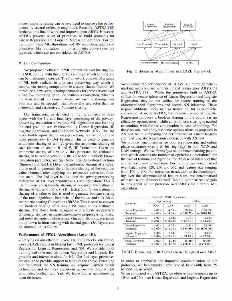
Our framework, as depicted in Fig. 1, consists of threelayers with the 3rd and final layer consisting of the privacy-preserving realization of various ML algorithms and formingthe end goal of our framework– i) Linear Regression, ii)Logistic Regression, and iii) Neural Networks (NN). The 3rdlayer builds upon the privacy-preserving realisation of 2ndlayer primitives– (i) Dot Product: This is used to generatearithmetic sharing of ~x � ~y, given the arithmetic sharing ofeach element of vectors ~x and ~y, (ii) Truncation: Given thearithmetic sharing of a value v, this generates the arithmeticsharing of truncated version of the value for a publicly knowntruncation parameter, and (iii) Non-linear Activation functions(Sigmoid and ReLU): Given the arithmetic sharing of a value,this is used to generate the arithmetic sharing of the resultantvalue obtained after applying the respective activation func-tion on it. The 2nd layer builds upon the privacy-preservingrealization of 1st layer primitives– (i) Multiplication: This isused to generate arithmetic sharing of x·y, given the arithmeticsharing of values x and y, (ii) Bit Extraction: Given arithmeticsharing of a value v, this is used to generate boolean sharingof the most significant bit (msb) of the value, and (iii) Bit toArithmetic sharing Conversion (Bit2A): This is used to convertthe boolean sharing of a single bit value to its arithmeticsharing. The above tools, designed with a focus on practicalefficiency, are cast in input-independent preprocessing phase,and input-dependent online phase. Our contributions, presentedin top-down fashion starting with the end-goals (3rd layer), canbe summed up as follows.

Performance of PPML Algorithms (Layer-III).– Relying on our efficient Layer-II building blocks, our frame-work BLAZE results in blazing fast PPML protocols for LinearRegression, Logistic Regression, and NN. We consider bothtraining and inference for Linear Regression and Logistic Re-gression and inference alone for NN. Our 2nd layer primitivesare enough to provide support to build all the above. Extendingour framework for NN training will require Garbled circuittechniques, and seamless transitions across the three worldsarithmetic, boolean and Yao. We leave this as an interestingopen direction.

LinearRegression

LogisticRegression

NeuralNetworks

Dot Product Truncation Sigmoid ReLU

Multiplication Bit Extraction Bit2A

Fig. 1: Hierarchy of primitives in BLAZE Framework

We illustrate the performance of BLAZE via thorough bench-marking and compare with its closest competitors ABY3 [5]and ASTRA [48]. While the primitives built in ASTRAsuffice for secure inference of Linear Regression and LogisticRegression, they do not suffice for secure training of theaforementioned algorithms and secure NN inference. Theserequire additional tools such as truncation, bit to arithmeticconversion. Also, in ASTRA, the inference phase of LogisticRegression produces a boolean sharing of the output (as anefficiency optimization), while an arithmetic sharing is neededto continue with further computation in case of training. Forthese reasons, we apply the same optimizations as proposed inASTRA while comparing the performance of Linear Regres-sion and Logistic Regression inferences with ASTRA.We provide benchmarking for both preprocessing and onlinephase separately over a 64-bit ring (Z2` ) in both WAN andLAN settings. We use throughput as the benchmarking param-eter, which denotes the number of operations (“iterations” forthe case of training and “queries” for the case of inference) thatcan be performed in unit time. For training, we benchmarkedover batch sizes 128, 256 and 512 and feature size rangingfrom 100 to 900. For inference, in addition to the benchmark-ing over the aforementioned feature sizes, we benchmarkedover real-world datasets as well. Table I summarizes the gainin throughput of our protocols over ABY3 for different MLalgorithms.

Layer-III: PPML Algorithms

AlgorithmPreprocessing Online

WAN LAN WAN LAN

Linear Regression(Training)

4.01×to 4.08×

4.01×to 4.08×

18.54×to 333.72×

138.89×to 2610.76×

Logistic Regression(Training)

1.97×to 2.96×

1.92×to 2.98×

6.13×to 53.19×

6.11×to 53.21×

Linear Regression(Inference)

4.02×to 5.00×

4.02×to 5.21×

2.81×to 194.86×

52.00×to 3600.00×

Logistic Regression(Inference)

1.32×to 2.36×

1.34×to 2.41×

3.18×to 27.52×

3.16×to 27.04×

Neural Networks(Inference)

4.02×to 4.07×

4.02×to 4.07×

65.46×to 276.31×

64.89×to 276.84×

TABLE I: Summary of BLAZE’s Gain in Throughput over ABY3

In order to emphasise the improved communication of ourprotocols, we benchmarked over varied bandwidth from 25to 75Mbps in WAN.When compared with ASTRA, we observe improvements up to194× and 15× over Linear Regression and Logistic Regression

3

inference respectively over WAN. The respective improve-ments over LAN are 1800× and 16×. Note that ASTRA hasnot considered the training of the above algorithms and NNinference.

Primary Building Blocks for PPML (Layer-II).– Dot Product: Dot Product forms the fundamental buildingblock for most of the ML algorithms and hence designingefficient constructions for the same are of utmost importance.We propose an efficient dot product protocol for which thecommunication in the online phase is independent of the sizeof the underlying vectors. Ours is the first solution in the three-party honest-majority and malicious setting, to achieve sucha result. Concretely, our solution requires communication of3n and 3 ring elements respectively in the preprocessing andonline phases, where n denotes the size of the underlyingvectors. When compared with the dot product protocol ofABY3, which requires communication of 12n and 9n ringelements in the preprocessing phase and online phase, ourprotocol results in the corresponding improvement of 4× and3n×. Similar comparison with ASTRA [48], which requirescommunication of 21n and 2n + 2 ring elements in thepreprocessing phase and online phase, our protocol results inrespective improvements of 7× and ≈ 0.67n×.– Truncation: For ML applications where the inputs arefloating-point numbers, the protocol for truncation plays a cru-cial role in determining the overall efficiency of the proposedsolution. Towards this, we propose an efficient truncationprotocol for the three server setting. When incorporated intoour dot product protocol, our truncation method adds a veryminimal overhead of just two ring elements in the preprocess-ing phase of the dot product protocol and more importantlykeeps its online complexity intact. In contrast, the state-of-the-art protocol of ABY3 requires expensive Ripple Carry Adder(RCA) circuits in the preprocessing phase which consumesrounds proportional to the underlying ring size. Moreover, theirsolution demands an additional round of communication with3 ring elements in the online phase.– Non-linear Activation functions: We provide efficient in-stantiation for Sigmoid and ReLU activation functions. Theformer is used in Logistic Regression, while the latter is usedin Neural Networks. Our constructions require only constantround of communication (≤ 4) in the online phase as opposedto ABY3. Moreover, we improve upon ABY3 in terms ofonline communication by a factor of ≈ 4.5×.

The performance comparison in terms of concrete cost forcommunication and round both for the preprocessing andonline phase of these primitives appear in Table II.

Layer-I: Secondary Building Blocks for PPML

– Multiplication: We propose a new and efficient multipli-cation protocol for the 3 server setting that can tolerate atmost one malicious corruption. Our construction invokes themultiplication protocol of [17] (which uses distributed ZeroKnowledge) in the preprocessing phase to facilitate an efficientonline phase. Concretely, our protocol requires an amortizedcommunication of 3 ring elements in both the preprocessingand online phases. Apart from the improvement in commu-nication, the asymmetric nature of our protocol enables oneamong the three servers to be idle majority of the time during

BuildingBlocks Ref.

Preprocessing Online

R C (`) R C (`)Layer-II: Building Blocks for PPML

Dot ProductABY3 4 12n 1 9n

ASTRA 6 21n 1 ≈ 2nBLAZE 4 3n 1 3

Dot Productwith Truncation

ABY3 2` - 2 ≈ 12n + 84 2 9n + 3BLAZE 4 3n + 2 1 3

Sigmoid ABY3 4 ≈ 108 log ` + 4 ≈ 81BLAZE 5 ≈ 5κ+ 23 5 ≈ κ+ 11

ReLU ABY3 4 60 log ` + 3 45BLAZE 5 ≈ 5κ+ 14 4 ≈ κ+ 7

Layer-I: Privacy-preserving Primitives

MultiplicationABY3 4 12 1 9

ASTRA 6 21 1 4BLAZE 4 3 1 3

BitExtraction

ABY3 4 24 1 + log ` 18ASTRA 7 46 3 ≈ 6BLAZE 4 9 1 + log ` 9BLAZE 5 ≈ 5κ+ 2 2 ≈ κ

Bit2A ABY3 4 24 2 18BLAZE 5 9 1 4

– Notations: ` - size of ring in bits, κ - computational security parameter,n - size of vectors for dot product, ‘R’ - number of rounds, ‘C’ - totalcommunication in units of ` bits.– ABY3, ASTRA and BLAZE requires an additional two rounds ofinteraction in the Online Phase for verification.

TABLE II: Comparison of ABY3 [5], ASTRA [48] and BLAZE interms of Communication and Round Complexity

the input-dependent phase. This construct serves as the primarybuilding block for our dot product protocol.While the multiplication protocol of [17] performs better thanours with a communication complexity of 3 ring elementsoverall yet in an amortized sense, we choose our construct overit mainly due to the huge benefits it brings for the case of dotproduct protocol. The dot product for n-length vectors can beviewed as n multiplications. Using [17] for the same will resultin a communication of 3n (amortized) ring elements in theonline phase. For the communication cost to get amortized, theprotocol of [17] requires a large number of multiplications tobe performed together, which cannot be guaranteed for severalinstances such as inference phases of Linear Regression andLogistic Regression. Furthermore, their protocol makes useof expensive public-key cryptography, which is undesirable insettings similar to ours, where practical efficiency is of utmostimportance in the online phase.On the other hand, our construct for multiplication whentweaked to obtain a dot product protocol requires communica-tion of 3n + 3 ring elements overall, where the preprocessingphase takes care of the expensive part involving invoking [17]and bearing heavy communication of 3n elements. This resultsin a blazing fast online phase for dot product which requirescommunication of just 3 ring elements and symmetric keyoperations. Lastly, as our setting calls for the computation ofmany multiplication operations in the preprocessing phase, theprotocol of [17] is used to perform them, and the communica-tion cost gets amortized over many multiplication operations.

– Bit Extraction: We provide two constructions based on thesolutions proposed by ASTRA [48] and ABY3 [5]. In thesolution based on ASTRA, servers use a garbled circuit thatcomputes a masked version of the most significant bit (MSB)of the input. This results in constant round complexity but the

4

communication will be dependent on the security parameterκ. On the other hand, the solution based on ABY3 results incommunication independent of κ but with a round complexityof 1 + log(`) where ` denotes the size of the underlying ringin bits.– Bit to Arithmetic sharing Conversion (Bit2A): The arithmeticequivalent of a bit b = b1 ⊕ b2 can be written as (b)A =(b1)A + (b2)A − 2(b1)A(b2)A. Here (b)A denotes the valueof bit b in ring Z2` . Thus the servers generate the arithmeticsharing of each of the shares of bit b and their product anduse the aforementioned relation to compute the final result.Our protocol, when compared to ABY3, gives 3× and 4×improvement with respect to the communication cost, in thepreprocessing and online phase, respectively.

The performance comparison of these primitives appear inTable II.

II. PRELIMINARIES AND DEFINITIONS

We consider a set of three servers P = {P0, P1, P2} thatare connected by pair-wise private and authentic channels ina synchronous network. We consider a static and Byzantineadversary, who can corrupt at most one of the three servers.In the case of ML training, many data-owners who wish tojointly train the model, secret-shares (as per schemes discussedlatter) their data amongst the three servers. In the case of MLinference, a model-owner and a client secret-share the trainedmodel and query respectively among the three servers. Once allthe inputs are available in shared fashion, servers perform thecomputation to generate the output in a shared format amongthem. For training, the output model is then reconstructed backto the data owners while for inference, the prediction resultis reconstructed towards the client alone. We assume that anarbitrary number of data owners can collude with the corruptserver for training, while for inference, either the model-owneror the client can collude with the corrupt server. The samesetting has been considered by ASTRA [48], ABY3 [5], andother related papers.

The ML algorithms to be evaluated (Layer-III), relevantto our setting, can be expressed as a circuit ckt with publiclyknown topology, consisting of the Layer-II gates– Dot Product,Truncation, Sigmoid, and ReLU. The gates in the Layer-IIare realized using the Layer-I primitives– Multiplication, BitExtraction, and Bit2A.

For a vector ~x, xi denotes the ith element in the vector. Fortwo vectors ~x and ~y of length n, the dot product is given by,~x � ~y =

∑ni=1 xiyi. Given two matrices X,Y, the operation

X ◦Y denotes the matrix multiplication.

a) Input-independent and Input-dependent Phases:The protocols of this work are cast into two phases: input-independent preprocessing phase and input-dependent onlinephase. This approach is useful in outsourced setting where theservers execute several instances of an agreed-upon function.The preprocessing for multiple instances can be executed inparallel. It is plausible for some of the protocols to have emptyinput-independent phase.

b) Shared Key Setup: To facilitate non-interactive com-munication, parties use a one-time key setup that establishespre-shared random keys for a pseudo-random function (PRF)

among them. A similar setup for the three-party case was usedin [4], [5], [8], [9], [48]. We model the above as functionalityFsetup (Fig. 17) and all our proofs are cast in Fsetup-hybridmodel.

c) Basic Primitives: In our protocols, we make use ofa collision-resistant hash function, denoted by H(), to savecommunication. Also, we use a commitment scheme, denotedby Com(), to boost the security of our constructions from abortto fairness. We defer the formal details of key setup, hashfunction, and the commitment scheme to Appendix A.

We use real-world / ideal-world simulation based approachto prove the security of our constructions and the details appearin Appendix F.

III. BUILDING LAYER-I PRIMITIVES

In this section, we start with the sharing semantics thatserve as the basis for all our primitives. The computationin each primitive is executed in shared fashion to obtain theprivacy-preserving property.

A. Secret Sharing Semantics

We use three types of secret sharing, as detailed below.

a) [·]-sharing: A value v ∈ Z2` is said to be [·]-sharedamong servers P1, P2, if the servers P1 and P2 respectivelyhold the values [v]1 ∈ Z2` and [v]2 ∈ Z2` such that v =[v]1 + [v]2.

b) 〈·〉-sharing: A value v ∈ Z2` is 〈·〉-shared amongservers in P , if– there exist [λv]1 , [λv]2 ∈ Z2` such that λv = [λv]1 + [λv]2.– P0 holds ([λv]1 , [λv]2), while Pi for i ∈ {1, 2} holds([λv]i , v + λv)

c) J·K-sharing: A value v ∈ Z2` is said to be J·K-sharedamong servers in P , if– v is 〈·〉-shared i.e. P0 holds ([αv]1 , [αv]2), while Pi for i ∈{1, 2} holds ([αv]i , βv) for αv, βv ∈ Z2` with βv = v + αv

and αv = [αv]1 + [αv]2– additionally, there exists γv ∈ Z2` such that P1, P2 hold γv,while P0 holds βv + γv.

The table below summarises the individual shares of theservers for the aforementioned secret sharings. [v]i, 〈v〉i andJvKi respectively denote the ith share held by Pi for [v], 〈v〉and JvK.

[v] 〈v〉 JvK

P0 − ([λv]1 , [λv]2) ([αv]1 , [αv]2 , βv + γv)

P1 [v]1 ([λv]1 , v + λv) ([αv]1 , βv = v + αv, γv)

P2 [v]2 ([λv]2 , v + λv) ([αv]2 , βv = v + αv, γv)

TABLE III: Shares held by the parties under different sharings

d) Arithmetic and Boolean Sharing: We use the sharingover both Z2` and Z21 and refer them as arithmetic andrespectively boolean sharing. The latter sharing is demarcatedusing a B in the superscript (e.g. JbKB).

5

e) Linearity of the secret sharing schemes: Given the[·]-sharing of x, y and public constants c1, c2, servers canlocally compute [c1x + c2y] as c1 [x] + c2 [y]. Notice thatlinearity trivially extends to the case of 〈·〉-sharing and J·K-sharing as well. Linearity allows the servers to perform the fol-lowing operations non-interactively: i) addition of two sharedvalues and ii) multiplication of the shared value with a publicconstant.

B. Secret Sharing and Reconstruction protocols

We dedicate this section to describe some of the secretsharing and reconstruction protocols that we need. We defer thecommunication complexity analysis and security proof of allthe constructs to Appendix C-A and Appendix F respectively.

a) Sharing Protocol: Protocol Πsh (Fig. 2) enablesserver Pi to generate J·K-sharing of value v ∈ Z2` . Duringthe preprocessing phase, servers P0, P1 along with Pi togethersample random value [αv]1, while servers P0, P2 and Pisample [αv]2 using the shared randomness. This enables serverPi to obtain the entire αv. Also, servers P1, P2 together samplea random γv ∈ Z2` . For the case when Pi = P0, we optimizethe protocol by making P0 sample the γv value along withP1, P2. This eliminates the need for servers P1, P2 to sendβv+γv to P0 during the online phase. Furthermore, the sharingdoes not need to hide the input from P0 (who is the inputcontributor) by keeping γv private.

During the online phase, Pi computes βv and sends it toP1, P2 who then verify the sanity of the received value byexchanging its hash with the fellow recipient. To completethe J·K-sharing, P1 sends βv + γv to P0 while P2 sends ahash of the same to P0, who aborts if the received valuesmismatch.

Preprocessing:

– If Pi = P0: Servers P0, Pj together sample random [αv]j ∈Z2` for j ∈ {1, 2}, while servers in P sample random γv ∈ Z2` .

– If Pi = P1: Servers P0, P1 together sample random [αv]1 ∈Z2` , while servers in P together sample random [αv]2 ∈ Z2` .Servers P1, P2 together sample random γv ∈ Z2` .

– If Pi = P2: Similar to the case of Pi = P1.

Online:

– Pi computes βv = v + αv and sends to both P1 and P2.

– If Pi = P0, servers P1, P2 mutually exchange H(βv) and abortif there is a mismatch.

– If Pi 6= P0, P1 computes and sends βv + γv to P0 while P2

sends a hash of the same to P0, who abort if the received valuesare inconsistent.

Protocol Πsh(Pi, v)

Fig. 2: J·K-sharing of a value v ∈ Z2` by server Pi

In the outsourced setting, input sharing is performed bythe parties and not the servers. Concretely, for the case ofML training, data owners perform the input sharing while forthe case of ML inference, input sharing is performed by themodel owner and the client. For a party P to perform the inputsharing of value v, server Pj for j ∈ {1, 2} sends [αv]j to P

while P0 sends a hash of the same to P . Party P computesαv = [αv]1 + [αv]2 if the received values are consistent andabort otherwise. P then computes βv = v + αv and sends toboth P1 and P2. The rest of the protocol proceeds similar toΠsh where servers P1, P2 mutually exchanges the hash of βvand verifies the consistency of βv.

b) Joint Sharing Protocol: Protocol Πjsh(Pi, Pj , v)(Fig. 3) enables servers Pi, Pj (an unordered pair) to jointlygenerate J·K-sharing of value v ∈ Z2` , known to both of them.Towards this, server Pi executes protocol Πsh on the value vto generate its J·K-sharing. Server Pj helps in verifying thecorrectness of the sharing performed by Pi.

– If (Pi, Pj) = (P1, P0): Server P1 executes protocol Πsh(P1, v).P0 computes βv = v +[αv]1 +[αv]2. P0 then sends H(βv) to P2

who aborts if the received value is inconsistent with the samereceived from P1.

– If (Pi, Pj) = (P2, P0): Similar to the case above.

– If (Pi, Pj) = (P1, P2): During the preprocessing phase, P1, P2

together sample random γv ∈ Z2` . Servers set [αv]1 = [αv]2 = 0and βv = v. P1 computes and sends v+γv to P0 while P2 sendscorresponding hash to P0, who aborts if the received values areinconsistent.

Protocol Πjsh(Pi, Pj , v)

Fig. 3: J·K-sharing of a value v ∈ Z2` by servers Pi, Pj

Protocol Πjsh can be made non-interactive for the casewhen the value v is available to both Pi and Pj in thepreprocessing phase. Towards this, servers in P sample randomr ∈ Z2` and locally set their shares as described in Table IV.Looking ahead, protocol Πjsh offers tolerance against oneactive corruption, leveraging the fact that the secret to beshared is available amongst two servers, with one of them isguaranteed to be honest.

(P1, P2) (P1, P0) (P2, P0)

[αv]1 = 0, [αv]2 = 0

βv = v, γv = r − v

[αv]1 = −v, [αv]2 = 0

βv = 0, γv = r

[αv]1 = 0, [αv]2 = −v

βv = 0, γv = r

P0

P1

P2

(0, 0, r )

(0, v, r − v)

(0, v, r − v)

(−v, 0, r)

(−v, 0, r)

( 0, 0, r)

(0, − v, r)

(0, 0, r)

(0, − v, r)

TABLE IV: The columns consider the three distinct possibilityof input contributing pairs. The first row shows the assignment tovarious components of the sharing. The last row (with three sub-rows) specifies the shares held by the three servers.

c) Reconstruction Protocol: Protocol Πrec(P, JvK)(Fig. 4) enables servers in P to reconstruct the secret v fromits J·K-sharing. Towards this, each server receives her missingshare from one of the other two servers and the hash of thesame from the third one. If the received values are consistent,the server proceeds with the reconstruction and otherwise,it aborts. Reconstruction towards a single server Pi can beviewed as a special case of this protocol and we use Πrec(Pi, v)to denote the same.

6

Online:

– P1 receives [αv]2 and H([αv]2) from P2 and P0 respectively.– P2 receives [αv]1 and H([αv]1) from P0 and P1 respectively.– P0 receives βv and H(βv) from P1 and P2 respectively.

Server Pi for i ∈ {0, 1, 2} abort if the received values areinconsistent. Else computes v = βv − [αv]1 − [αv]2.

Protocol Πrec(P, JvK)

Fig. 4: Reconstruction of value v ∈ Z2` among servers in P

In the outsourced setting where reconstruction happens towardsthe parties (data owners for ML training and client for MLinference), the servers will send their shares towards the partiesdirectly. To reconstruct a value v towards party P , serversP0, P1 and P2 sends (JαvKA,H(JαvKB)), (βv,H(JαvKA)) and(JαvKB,H(βv)) respectively to P . Party P will accept theshares if the corresponding hash match and abort otherwise.

d) Fair Reconstruction Protocol: The security goal offairness is well-motivated. Consider an outsourced settingwhere a machine learning service that is instantiated with aprotocol with abort is offered against payment. Here, duringthe reconstruction of output, adversary can instruct the corruptserver to send inconsistent values (either shares or hash values)to honest parties and make them abort. At the same time,adversary will learn the output from the honest shares receivedon behalf of the corrupt parties. This leads to a situationwhere some parties who have control over the corrupt serverobtain the protocol output, while the other honest parties obtainnothing. This is a strong deterrent for the honest parties toparticipate in the protocol in the future. On the other hand,a system with fairness property guarantees that the honestparties will get the output whenever the corrupt parties getsthe output. In our 3PC setting, the presence of at least a singlehonest server ensures that all the participating honest partieswill eventually get the output. This will attract more people toparticipate in the protocol and is crucial to applications likeML training where more data leads to a better-trained model.

We use the techniques proposed by ASTRA [48] to achievefairness and modify it for our sharing scheme. We defer formaldetails to the appendix (Section C-A4).

C. Layer-I Primitives

We are now ready to describe our Layer-I primitives–Multiplication, Bit Extraction, and Bit2A. We defer the com-munication complexity analysis and security proof of all theconstructs to Appendix C-B and Appendix F respectively.

a) Multiplication Protocol: Protocol Πmult(P, JxK, JyK)enables the servers in P to compute J·K-sharing of z = xy,given the J·K-sharing of x and y. We begin with a protocol forthe semi-honest setting, which is a slightly modified variant ofthe protocol proposed by ASTRA. During the preprocessingphase, P0, Pj for j ∈ {1, 2} sample random [αz]j ∈ Z2` ,while P1, P2 sample random γz ∈ Z2` . In addition, P0 locallycomputes Γxy = αxαy and generates [·]-sharing of the samebetween P1, P2. Since

βz = z + αz = xy + αz = (βx − αx)(βy − αy) + αz

= βxβy − βxαy − βyαx + Γxy + αz (1)

holds, servers P1, P2 locally compute [βz]j = (j−1)βxβy−βx [αy]j − βy [αx]j + [Γxy]j + [αz]j during the online phaseand mutually exchange their shares to reconstruct βz. ServerP1 then computes and sends βz + γz to P0, completing thesemi-honest protocol. The correctness that asserts z = xy orin other words βz − αz = xy holds due to Equation 1.

In the malicious setting, we observe that the aforemen-tioned protocol suffers from three issues:

1. When P0 is corrupt, the [·]-sharing of Γxy performed byP0 during the preprocessing phase might not be correct,i.e. Γxy 6= αxαy.

2. When P1 (or P2) is corrupt, the [·]-share of βz handedover to the fellow honest evaluator during the onlinephase might not be correct, causing reconstruction of anincorrect βz.

3. When P1 is corrupt, the value βz + γz that is sent to P0

during the online phase may not be correct.

While the first two issues in the above list are inheritedfrom the protocol of ASTRA, the third one is due to our newsharing semantics (compared to ASTRA where γv and βv +γv were not part of the shares) that imposes an additionalcomponent of βz + γz held by P0. We begin with solving thelast issue first. In order to verify the correctness of βz + γzsent by P1, server P2 computes a hash of the same and sendit to P0, who aborts if the received values are inconsistent.

For the remaining two issues, though they are quite distinctin nature, we make use of the asymmetric roles played bythe servers {P0} and {P1, P2} to introduce a single checkthat solves both the issues at the same time. Though thecheck is inspired from the protocol of ASTRA, our technicalinnovation lies in the way in which the check is performed. InASTRA, servers first execute the semi-honest protocol and thecorrectness of the computation is verified with the help of 〈·〉-sharing of a multiplication triple generated in the preprocessingphase. Unlike ASTRA, we perform a single multiplication (andnothing additional) in the preprocessing phase to generate thecorrect preprocessing data required for a multiplication gatein the online phase. This brings down the communication inthe preprocessing phase drastically from 21 ring elements to3 ring elements. The details of our method are provided next.

To solve the second issue, where a corrupt P1 (or P2)sends an incorrect [·]-share of βz, we make use of server P0

as follows: Using the values β?x = βx + γx and β?y = βy + γy,P0 computes β?z = −β?xαy − β?yαx + 2Γxy + αz. Now β?z canbe written as below:

β?z = −β?xαy − β?yαx + 2Γxy + αz

= −(βx + γx)αy − (βy + γy)αx + 2Γxy + αz

= (−βxαy − βyαx + Γxy + αz)− (γxαy + γyαx − Γxy)

= (βz − βxβy)− (γxαy + γyαx − Γxy + ψ) + ψ [Equation 1]

= (βz − βxβy + ψ)− χ [where χ = γxαy + γyαx − Γxy + ψ]

Assuming that (a) ψ ∈ Z2` is a random value sampledtogether by P1 and P2 (and unknown to P0) and (b) P0 knowsthe value χ, P0 can send β?z + χ to P1 and P2 who using theknowledge of βx, βy and ψ can verify the correctness of βzby computing βz − βxβy + ψ and checking against the valueβ?z + χ received from P0. Now we describe how to enableP0 to obtain the value χ. Note that server Pj for j ∈ {1, 2}

7

can locally compute [χ]j = γx [αy]j + γy [αx]j − [Γxy]j + [ψ]jwhere [ψ]j can be generated non-interactively by P1, P2 usingshared randomness. P1, P2 can then send their [·]-shares ofχ to P0 to enable him obtain the value χ. To verify if P0

computed χ correctly, we leverage the following relation. Thevalues d = γx − αx, e = γy − αy and f = (γxγy + ψ) − χshould satisfy f = de if and only if χ is correctly computed,because:

de = (γx − αx)(γy − αy) = γxγy − γxαy − γyαx + Γxy

= (γxγy + ψ)− (γxαy + γyαx − Γxy + ψ)

= (γxγy + ψ)− χ = f

Therefore, the correctness of χ reduces to verifying if thetriple (d, e, f) is a multiplication triple or not. Interestingly,the same check suffices to resolve the first issue of corrupt P0

generating incorrect [Γxy]-sharing. This is because, if P0 wouldhave shared Γxy + ∆ where ∆ denotes the error introduced,then de = f + ∆ 6= f.

Equipped with the aforementioned observations (Table V),our final trick, that distinguishes BLAZE’s multiplication fromthat of ASTRA’s, is to compute a 〈·〉-sharing of f startingwith 〈·〉-sharing of d, e using the efficient maliciously securemultiplication protocol of [17] referred to as ΠmulZK henceforthand described in Appendix B for completeness, and extractout the values for Γxy, ψ and χ from f which are bound tobe correct. This can be executed entirely in the preprocessingphase. Protocol ΠmulZK works over 〈·〉-sharing (Section III-A),which is why this part our computation is done over this typeof sharing, and requires a per party communication of 1 ringelement, when amortized over large circuits (ref. Theorem 1.4of [17]1). Concretely, given the J·K-sharing of the inputs x andy of the multiplication protocol, servers locally compute 〈·〉-sharing of values d and e as follows. (The sharing semanticsfor [v] for any v is recalled below.)

P0 P1 P2

〈v〉 ([λv]1 , [λv]1) ([λv]1 , v + λv) ([λv]2 , v + λv)

〈d〉 ([αx]1 , [αx]2) ([αx]1 , γx) ([αx]2 , γx)

〈e〉 ([αy]1 , [αy]1) ([αy]1 , γy) ([αy]2 , γy)

TABLE V: The 〈·〉-sharing of values d and e

Upon executing protocol ΠmulZK(P, d, e), servers obtain〈f〉 = ([λf ] , f + λf). To be precise, P0 obtains ([λf ]1 , [λf ]2)while Pj for j ∈ {1, 2} obtains ([λf ]j , f + λf). Servers thenmap the values [χ] and γxγy +ψ to [λf ] and f +λf respectivelyfollowed by extracting the required values as:

[χ]1 = [λf ]1 and [χ]2 = [λf ]2 → χ = [λf ]1 + [λf ]2γxγy + ψ = f + λf → ψ = f + λf − γxγy

[Γxy]j = γx [αy]j + γy [αx]j + [ψ]j − [χ]j [j ∈ {1, 2}]

where [ψ] is generated non-interactively by servers P1, P2

by sampling a random value r ∈ Z2` together and setting[ψ]1 = r and [ψ]2 = ψ − r. We claim that after extracting thevalues as mentioned above, servers P1, P2 hold [Γxy] = [αxαy].To see this, note that

1https://eprint.iacr.org/2019/188

Γxy = γxαy + γyαx + ψ − χ= (d + λd)λe + (e + λe)λd + (f + λf − γxγy)− λf= (d + λd)(e + λe)− de + λdλe + (f − γxγy)= γxγy − f + λdλe + (f − γxγy) = λdλe = αxαy

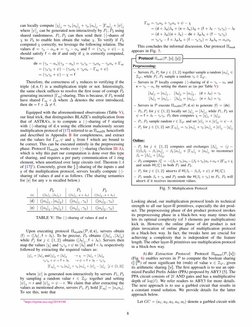
This concludes the informal discussion. Our protocol Πmult

appears in Fig. 5.

Preprocessing:

– Servers P0, Pj for j ∈ {1, 2} together sample a random [αz]j ∈Z2` , while P1, P2 sample a random γz ∈ Z2` .

– Servers in P locally compute 〈·〉-sharing of d = γx − αx ande = γy − αy by setting the shares as (as per Table V):

[λd]1 = [αx]1 , [λd]2 = [αx]2 , (d + λd) = γx

[λe]1 = [αy]1 , [λe]2 = [αy]2 , (e + λe) = γy

– Servers in P execute ΠmulZK(P, d, e) to generate 〈f〉 = 〈de〉.– P0, Pj for j ∈ {1, 2} locally set [χ]j = [λf ]j , while P1, P2 setψ = f + λf − γxγy. P0 then computes χ = [χ]1 + [χ]2.

– P1, P2 sample random r ∈ Z2` and set [ψ]1 = r, [ψ]2 = ψ− r.

– Pj for j ∈ {1, 2} set [Γxy]j = γx [αy]j + γy [αx]j + [ψ]j − [χ]j

Online:

– Pj for j ∈ {1, 2} computes and exchanges [βz]j = (j −1)βxβy − βx [αy]j − βy [αx]j + [Γxy]j + [αz]j to reconstructβz = [βz]1 + [βz]2.

– P0 computes β?z = −(βx+γx)αy−(βy +γy)αx+αz+2Γxy +χ

and sends H(β?z ) to both P1 and P2.

– Pj for j ∈ {1, 2} aborts if H(βz − βxβy + ψ) 6= H(β?z ).

– P1 sends βz + γz and P2 sends the H(βz + γz) to P0. P0 willabort if it receives inconsistent values.

Protocol Πmult(P, JxK, JyK)

Fig. 5: Multiplication Protocol

Looking ahead, our multiplication protocol lends its technicalstrength to all our layer-II primitives, especially the dot prod-uct. The preprocessing phase of dot product protocol invokesits preprocessing phase in a black-box way many times thatlets its optimal complexity (of 3 elements per multiplication)kick in. However, the online phase of dot product is notplain invocation of online phase of multiplication protocolin a black-box way. In fact, the tweaks here are crucial forachieving a complexity that is independent of the featurelength. The other layer-II primitives use multiplication protocolin a block-box way.

b) Bit Extraction Protocol: Protocol Πbitext(P, JvK)(Fig. 6) enables servers in P to compute the boolean sharing(J·KB) of most significant bit (msb) of value v ∈ Z2` , givenits arithmetic sharing JvK. The first approach is to use an opti-mized Parallel Prefix Adder (PPA) proposed by ABY3 [5]. ThePPA circuit consists of 2` AND gates and has a multiplicativedepth of log(`). We refer readers to ABY3 for more details.The next approach is to use a garbled circuit that results ina constant round solution. We provide details for the latterapproach below.

Let GC = (u1, u2, u3, u4, u5) denote a garbled circuit with

8

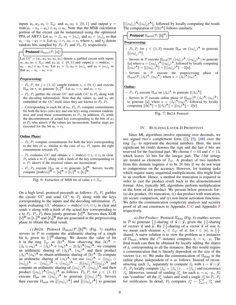
inputs u1, u2, u3 ∈ Z2` and u4, u5 ∈ {0, 1} and output y =msb(u1 − u2 − u3)⊕ u4 ⊕ u5. Note that the MSB calculationportion of the circuit can be instantiated using the optimizedPPA of ABY3. Let u1 = βv, u2 = [αv]1 and u3 = [αv]2 so thatu1−u2−u3 = v. Let u4 = r1, u5 = r2 where r1 and r2 denoterandom bits sampled by P0, P1 and P0, P2 respectively.

Let GC = (u1, u2, u3, u4, u5) denote a garbled circuit with inputsu1, u2, u3 ∈ Z2` and u4, u5 ∈ {0, 1} and output y = msb(u1 −u2 − u3) ⊕ u4 ⊕ u5. Let u1 = βv, u2 = [αv]1 and u3 = [αv]2 sothat u1 − u2 − u3 = v.

Preprocessing:

– P0, Pj for j ∈ {1, 2} sample random rj ∈ {0, 1} and executeΠjsh on rj to generate JrjKB. Let u4 = r1 and u5 = r2.

– P0, P1 garbles the circuit GC and sends GC to P2 along withthe decoding information. Note that the values u2 and u4 areembedded in the GC itself since they are known to P0, P1.

– Corresponding to each bit of u3, P0, P1 compute commitmentsfor both the keys (zero key and one key) using common random-ness and send these commitments to P2. In addition, P0 sendsthe decommitment of actual key corresponding to the bits of u3

to P2 who abort if the values are inconsistent. Similar steps areexecuted for the bit u5 = r2.

Online Phase:

– P0, P1 compute commitments for both the keys correspondingto the bits of u1 similar to the case of u3. P1 opens the rightcommitment towards P2.

– P2 evaluates GC and obtains v = msb(v) ⊕ r1 ⊕ r2 in clear.P2 sends v to P1 along with a hash of the key corresponding tov. P1 abort if the received values are inconsistent.

– P1, P2 execute Πjsh on v to generate JvKB. Servers locallycompute Jmsb(v)KB = JvKB ⊕ Jr1KB ⊕ Jr2KB.

Protocol Πbitext(P, JvK)

Fig. 6: Extraction of MSB bit of value v ∈ Z2`

On a high level, protocol proceeds as follows: P0, P1 garblesthe circuit GC and send GC to P2 along with the keyscorresponding to the inputs and the decoding information. P2

upon evaluating GC obtains v = msb(v)⊕ r1⊕ r2 in clear andsends v along with a hash of the actual key corresponding tov to P1. P1, P2 then jointly generate JvKB. Servers then XORJvKB to Jr1KB and Jr2KB that are generated in the preprocessingphase to obtain the final result.

c) Bit2A: Protocol Πbit2A(P, JbKB) (Fig. 7) enablesservers in P to compute the arithmetic sharing of a singlebit b, given its J·KB-sharing. We denote the value of bitb in the ring Z2` as (b)A. Now observing that (b)A =(βb ⊕ αb)

A = (βb)A + (αb)

A − 2(βb)A(αb)

A, we computean arithmetic sharing of (βb)

A, (αb)A and their product

(βb)A(αb)

A to obtain arithmetic sharing of (b)A. To computean arithmetic sharing of (αb)

A, we use (αb)A = ([αb]1 ⊕

[αb]2)A = ([αb]1)A + ([αb]2)A − 2([αb]1)A([αb]2)A andcompute an arithmetic sharing of ([αb]1)A, ([αb]2)A and theirproduct ([αb]1)A([αb]2)A as follows. P0, Pj for j ∈ {1, 2}execute Πjsh on ([αb]j)

A to generate J([αb]j)AK. Servers

then execute Πmult on J([αb]1)AK and J([αb]2)AK to generate

J([αb]1)A([αb]2)AK, followed by locally computing the result.The computation of J(b)AK follows similarly.

Preprocessing:

– P0, Pj for j ∈ {1, 2} execute Πjsh on ([αb]j)A to generate

J([αb]j)AK.

– Servers in P execute Πmult(P, ([αb]1)A, ([αb]2)A) to generateJuK where u = ([αb]1)A([αb]2)A, followed by locally computingJ(αb)

AK = J([αb]1)AK + J([αb]2)AK− 2JuK.

– Servers in P execute the preprocessing phase ofΠmult(P, (βb)A, (αb)

A) where v = (βb)A(αb)

A.

Online:

– P1, P2 execute Πjsh on (βb)A to generate J(βb)AK.

– Servers in P execute online phase of Πmult(P, (βb)A, (αb)A)

to generate JvK where v = (βb)A(αb)

A, followed by locallycomputing J(b)AK = J(βb)AK + J(αb)

AK− 2JvK.

Protocol Πbit2A(P, JbKB)

Fig. 7: Bit2A Protocol

IV. BUILDING LAYER-II PRIMITIVES

Since ML algorithms involve operating over decimals, weuse signed two’s complement form [2], [5], [48] over thering Z2` to represent the decimal numbers. Here, the mostsignificant bit (msb) denotes the sign and the last d bits arereserved for the fractional part. We choose ` = 64 and d = 13,which leaves 50 bits for the integer part. The `-bit stringsare treated as elements of Z2` . A product of two numbersfrom this domain requires d to be 26 bits if we do not wantto compromise on the accuracy. However, for training taskswhich require many sequential multiplications, this might leadto an overflow. Hence, a method for truncation is required inorder to cast the product result back in the aforementionedformat. Also, typically ML algorithms perform multiplicationin the form of dot product. We present below protocols for–(a) dot product, (b) truncation, (c) dot product with truncation,(d) secure comparison, and (e) non-linear activation functions.We defer the communication complexity analysis and securityproof of all our constructs to Appendix C-C and Appendix Frespectively.

a) Dot Product: Protocol Πdotp (Fig. 8) enables serversin P to generate J·K-sharing of ~x � ~y, given the J·K-sharingof vectors ~x and ~y. By J·K-sharing of a vector ~x of size n,we mean each element xi ∈ Z2` of it, for i ∈ [n], is J·K-shared. A naive solution is to view the problem as n instancesof Πmult, where the ith instance computes zi = xi · yi. Thefinal result can then be obtained by locally adding the sharesof zi corresponding to all the instances. But this would requirea communication that is linearly dependent on the size of thevectors (i.e. n). We make the communication of Πdotp in theonline phase independent of n as follows: Instead of recon-structing each βzi separately to compute βz with z = ~x � ~y,P1, P2 locally compute [βz] = [βz1 ]+. . .+[βzn ] and reconstructβz. Moreover, instead of sending β?zi for each zi = xi · yi, P0

can “combine” all the β?zi values and send a single β?z to P1, P2

for verification. In detail, P0 computes β?z =∑ni=1 β

?zi and

9

sends a hash of the same to both P1 and P2, who then can crosscheck with a hash of βz−

∑ni=1(βxi ·βyi−ψi).

Preprocessing:

– Servers in P execute preprocessing phase of Πmult(P, xi, yi)for each pair (xi, yi) where i ∈ [n] and zi = xiyi. P0 obtainsχi, while Pj , for j ∈ {1, 2}, obtains [Γxiyi ]j and ψi.

– P0 computes χ =∑n

i=1 χi,Γxy =∑n

i=1 Γxiyi , while Pj forj ∈ {1, 2} computes [Γxy]j =

∑ni=1 [Γxiyi ]j , ψ =

∑i ψi.

– P0, Pj for j ∈ {1, 2} compute [αz]j =∑n

i=1 [αzi ]j .

Online Phase:

– Pj for j ∈ {1, 2} computes [βz]j =∑n

i=1((j − 1)βxiβyi −βxi [αyi ]j − βyi [αxi ]j) + [Γxy]j + [αz]j and mutually exchanges[βz]j to reconstruct βz.

– P0 computes β?z = −

∑ni=1(βxi + γxi)αyi −

∑ni=1(βyi +

γyi)αxi + αz + 2Γxy + χ and sends H(β?z ) to P1, P2.

– Pj for j ∈ {1, 2} abort if H(β?z ) 6= H(βz−

∑ni=1 βxiβyi +ψ).

– P1 sends βz + γz and P2 sends the H(βz + γz) to P0. P0 willabort if it receives inconsistent values.

Protocol Πdotp(P, {JxiK, JyiK}i∈[n])

Fig. 8: Dot Product Protocol

b) Truncation: A truncation protocol enables theservers to compute JvdK from JvK, where vd denotes thetruncated value of v (right-shifted value of v by d bit positions,where d is the number of bits allocated for the fractionalpart). SecureML [2] proposed an efficient truncation methodfor 2 parties where the parties locally truncate their sharesafter every multiplication. ABY3 [5] showed that this methodfails when extended to 3-party, and proposed an alternativeway using a shared truncated pair (r, rd), for a random r,to achieve truncation. Their method of truncating the sharesof the product after evaluating a multiplication gate preservesthe underlying truncated value with very high probability. Wefollow the technique of ABY3 and primarily differ in the wayin which (r, rd) is generated. With the random truncation pair(r, rd) and a value v to be truncated, both available in J·K-sharedform, the truncated v in J·K-shared format can be obtained byopening (v− r), truncating it and then adding it to JrdK. Belowwe present a protocol that prepares the random truncation pair.

– P0, Pj for j ∈ {1, 2} sample random Rj ∈ Z2` . P0 sets r =R1 + R2 while Pj sets [r]j = Rj . Pj sets [rd]j as the ringelement that has last d bits of rj in the last d positions and 0elsewhere.

– P0 locally truncates r to obtain rd and executes Πsh(P0, rd) to

generate JrdK. P1 locally sets[rd]1

= βrd − [αrd ]1, while P2

sets[rd]2

= − [αrd ]2.

– P1 computes u = [r]1−2d[rd]1− [rd]1 and sends H(u) to P2.

– P2 locally computes v = 2d[rd]2

+ [rd]2 − [r]2 and abort ifH(u) 6= H(v).

Protocol Πtrgen(P)

Fig. 9: Generating Random Truncated Pair (r, rd)

Protocol Πtrgen(P) (Fig. 9) generates a pair ([r] , JrdK) for arandom r. Servers P0, Pj for j ∈ {1, 2} sample random value

Rj ∈ Z2` followed by P0 locally truncating r = R1 + R2

to obtain rd. Note that r = 2drd + rd where rd denotes thering element that has last d bits of r in the last d positionsand 0 elsewhere. P0 then generates JrdK by executing thesharing protocol Πsh. To verify the correctness of sharingperformed by P0, servers P1, P2 compute a [·]-sharing ofa = (r − 2drd + rd), given ([r] , JrdK) and checks if a = 0. Tooptimize communication, P1 sends a hash of his share H([a]1)to P2, who aborts if the received hash value mismatches withH(− [a]1).

To see the correctness, it suffices to show that u = v whereu = [r]1 − 2d

[rd]1− [rd]1 and v = 2d

[rd]2

+ [rd]2 − [r]2. Westart from the observation that r = 2drd + rd.

r = 2drd + rd

[r]1 + [r]2 = 2d([rd]P1

+[rd]P2

) + ([rd]P1+ [rd]P2

)

[r]1 − 2d[rd]1− [rd]1 = 2d

[rd]2

+ [rd]2 − [r]2u = v

Πtrgen(P) can entirely be run in the preprocessing phase. Ourdot product with truncation, presented below, will invoke it inthe preprocessing phase.

c) Dot Product with Truncation: Protocol Πdotpt(P,{JxiK, JyiK}i∈[n]) (Fig. 10) enables servers in P to generate J·K-sharing of truncated value of z = ~x� ~y denoted as zd, giventhe J·K-sharing of vectors ~x and ~y. To achieve the goal, wemodify our dot product protocol Πdotp in a way that does notinflate the online cost. This is unlike ABY3, which requiresan additional reconstruction in the online phase.

In the preprocessing phase, along with the steps of Πdotp,the servers execute Πtrgen to generate a truncation pair (r, rd).In the online phase, the servers P1, P2 locally compute [·]-sharing of (z − r) (instead of [βz]) where z = ~x � ~y. Thisis followed by P1, P2 locally truncating (z − r) to obtain(z− r)d and generating J·K-sharing of the same by executingΠjsh protocol. Finally, the servers locally compute J·K-sharingof z by adding the shares of (z− r)d and JrdK. To ensure thecorrectness of the computation, the steps of P0 are modifiedsuch that P0 will be computing (z− r)? instead of β?z .

Preprocessing:

– Servers in P execute preprocessing phase ofΠdotp(P, {JxiK, JyiK}i∈[n]).

– In parallel, servers execute Πtrgen(P) to generate the truncationpair ([r] , JrdK). Moreover P0 obtains the value r in clear.

Online:

– Pj for j ∈ {1, 2} computes [(z− r)]j = [z]j−[r]j where [z]j =[βz]j − [αz]j =

∑ni=1((j− 1)βxiβyi −βxi [αyi ]j −βyi [αxi ]j) +

[Γxy]j .

– Pj for j ∈ {1, 2} mutually exchange [(z− r)]j to reconstruct(z− r), followed by locally truncating it to obtain (z− r)d.

– P1, P2 execute Πjsh(P1, P2, (z− r)d) to generate J(z− r)dK.

– Servers in P locally compute JzK = J(z− r)dK + JrdK– P0 computes Ψ = −

∑ni=1(βxi + γxi)αyi −

∑ni=1(βyi +

γyi)αxi +2Γxy− r, sets (z− r)? = Ψ+χ and sends H((z− r)?)to both P1 and P2.

Protocol Πdotpt(P, {JxiK, JyiK}i∈[n])

10

– Pj for j ∈ {1, 2} aborts if H((z− r)−∑n

i=1 βxiβyi + ψ) 6=H((z− r)?).

Fig. 10: Dot Product Protocol with Truncation

d) Secure Comparison: Given two values x, y ∈ Z2` inJ·K-shared format, secure comparison allows parties to checkwhether x < y or not. In fixed-point arithmetic representation,this can be accomplished by checking the sign of v = x −y, which is stored in its msb position. Towards this, serverslocally compute JvK = JxK − JyK followed by extracting themsb using protocol Πbitext on JvK. For the cases that demandthe result in arithmetic sharing format, servers can apply theBit2A protocol Πbit2A on the outcome of Πbitext.

e) Activation Functions: We consider two widely usedactivation functions– i) Rectified Linear Unit (ReLU) and ii)Sigmoid (Sig).

– ReLU: The ReLU function, defined as relu(v) =max(0, v) can be viewed as relu(v) = b ·v where the bit b = 1if v < 0 and 0 otherwise. Here b denotes the complement ofbit b. Protocol Πrelu(P, JvK) enables servers in P to computeJ·K-sharing of relu(v) given the J·K-sharing of v ∈ Z2` .

For this, servers first execute the msb extraction protocolΠbitext on v to obtain JbKB. Given JbKB, servers locallycompute JbKB by setting βb = 1 ⊕ βb. Servers then executeBit2A protocol Πbit2A on JbKB to generate JbK. Lastly, serversexecute multiplication protocol Πmult on b and v to generateJ·K-sharing of the result.

– Sig: We use the MPC-friendly version of the Sigmoidfunction [2], [5], [48], which is defined as:

sig(v) =

0 v < − 12

v + 12 − 1

2 ≤ v ≤ 12

1 v > 12

Note that sig(v) = b1b2(v + 1/2) + b2, where b1 = 1 ifv + 1/2 < 0 and b2 = 1 if v− 1/2 < 0. Protocol Πsig(P, JvK)is similar to that of Πrelu and therefore we omit the details.

V. BUILDING PPML AND BENCHMARKING

We consider three widely used ML algorithms for ourbenchmarking and compare with their closest competitors–i) Linear Regression (training and inference), ii) LogisticRegression (training and inference) and iii) Neural Networks(inference). Training for NN requires conversions to and fromGarbled Circuits (for tackling some functions) which are notconsidered in this work. To obtain fairness in our protocols, thefinal outcome is reconstructed via fair reconstruction protocolΠfrec(P, JvK) (Fig. 21). In addition to the above, we alsobenchmark the dot product protocol separately as it is a majorbuilding block for PPML. We start with the experimental setup.

a) Benchmarking Environment: We use a 64-bit ring(Z264 ). The benchmarking is performed over a LAN of 1Gbpsbandwidth and a WAN of 75Mbps bandwidth. Over the LAN,we use machines equipped with 3.6 GHz Intel Core i7-7700CPU processor and 32 GB of RAM Memory. The WAN was

instantiated using n1-standard-8 instances of Google Cloud2

with machines located in East Australia (P0), South Asia(P1) and South East Asia (P2). Over the WAN, machines areequipped with 2.3 GHz Intel Xeon E5 v3 (Haswell) processorssupporting hyper-threading, with 8 vCPUs, and 30 GB ofRAM Memory. The average round-trip time (rtt) was takenas the time for communicating 1 KB of data between a pair ofparties. Over the LAN, the rtt turned out to be 0.296ms. Inthe WAN, the rtt values for the pairs P0-P1, P0-P2 and P1-P2

are 152.3ms, 60.19ms and 92.63ms respectively.

b) Software Details: We implement our protocols usingthe publicly available ENCRYPTO library [49] in C++17.We implemented the code of ABY3 [5] and ASTRA [48] inour environment since they were not publicly available. Thecollision-resistant hash function was instantiated using SHA-256. We have used multi-threading and our machines werecapable of handling a total of 32 threads. Each experiment isrun for 20 times and the average values are reported.

c) Benchmarking Parameter: We use throughput (TP)as the benchmarking parameter following ABY3 [5] andASTRA [48] as it would help to analyse the effect of improvedcommunication and round complexity in a single shot. HereTP denotes the number of operations (“iterations” for thecase of training and “queries” for the case of inference) thatcan be performed in unit time. We consider minute as theunit time since most of our protocols over WAN requiresmore than a second to complete. To analyse the performanceof our protocols under various bandwidth settings, we reportthe performance under the following bandwidths: 25 Mbps,50Mbps and, 75Mbps.

We provide the benchmarking for the WAN setting belowand defer the same for the LAN setting to Appendix E.

A. Dot Product

Here the throughput is computed as the number of dotproducts performed per minute (#dotp/min) and the same iscomputed for both preprocessing and online phases separately.

100200300400500600700

0

2

4

6

8·105

Feature Size

Prep

roce

ssin

gT

P(#

dotp

/min

ute)

BLAZE - 25 MbpsBLAZE - 50 MbpsBLAZE - 75 Mbps

ABY3 - 25 MbpsABY3 - 50 MbpsABY3 - 75 Mbps

(a) Preprocessing TP

200 400 600 800

0

200

400

600

800

1,000

1,200

Feature Size

Gai

nin

Onl

ine

TP

over

AB

Y3

25 Mbps50 Mbps75 Mbps

(b) Online TP

Fig. 11: Throughput (TP) Comparison of ABY3 and BLAZE overvarying Bandwidths

For the preprocessing phase, we plot the throughput of thedot product protocol of BLAZE (Fig. 11a) and ABY3 overvectors of length ranging from 100 to 1000. We note at leasta gain of 4×, which is a consequence of 4× improvement incommunication, over ABY3. An interesting observation to be

2https://cloud.google.com/

11

made here is that our protocol, over the bandwidth of 25Mbps,gives better throughput when compared to ABY3 even over ahigher bandwidth of 75Mbps.

For the online phase (Fig. 11b), we plot the gain overABY3 in terms of throughput. We observe an appreciable gainin throughput which is a direct corollary of the communica-tion cost our protocol being independent of the vector size.Concretely, for a bandwidth of 50 Mbps, our gain ranges from64× to 580×. Note that, with an increase in bandwidth thereis a drop in the gain. This is because even at a bandwidth of 25Mbps the maximum attainable throughput cannot be handledby our processors. For a bandwidth of 8 Mbps, the maximumattainable throughput is within our processing capacity, wherewe observe throughput gain ranging from 400× to 3600×. Thisshowcases the practicality of our constructions over low-endnetworks.

In the preprocessing phase, over all the bandwidths underconsideration, the maximum attainable throughput lies wellwithin the processing capacity of our machines. Consequen-tially, we do not observe a drop in the throughput gain withincreasing bandwidth, as is seen in the online phase. This isthe reason why we choose to plot the actual throughput valuesinstead of the gain in the case of the preprocessing phase. Onincreasing the processing capacity we expect a consistent gainin online throughput with increasing bandwidth.

B. ML Training

In this section, we explore the training phase of LinearRegression and Logistic Regression algorithms. The trainingphase can be divided into two stages– (i) a forward propa-gation phase, where the model computes the output given theinput; (ii) a backward propagation phase, where the modelparameters are adjusted according to the difference in thecomputed output and the actual output. For our benchmarking,we define one iteration in the training phase as one forwardpropagation followed by a backward propagation. Our perfor-mance improvement over ABY3 is reported in terms of thenumber of iterations over feature size varying from 100 to1000, and a batch size of B ∈ {128, 256, 512}. Batching [2],[5] is a common optimization where n samples are divided intobatches of size B and a combined update function is appliedto the weight vectors. In order to analyse the performanceover a wide range of features and batch sizes, we choose tobenchmark over synthetic datasets following ABY3 [5].

a) Linear Regression: In Linear Regression, one it-eration comprises of updating the weight vector ~w using thegradient descent algorithm (GD). It is updated according tothe following function:

~w = ~w − α

BXTi ◦ ((Xi ◦ ~w)−Yi)

where α denotes the learning rate and Xi denotes a subsetof batch size B, randomly selected from the entire dataset inthe ith iteration. The forward propagation involves computingXi ◦ ~w, while the backward propagation consists of updatingthe weight vector. The update function requires computationof a series of matrix multiplications, which can be achievedusing dot product protocols. The update function, as mentioned

earlier, can be computed entirely using J·K shares as:

J~wK = J~wK− α

BJXT

j K ◦ ((JXjK ◦ J~wK)− JYjK)

The operations of subtraction as well as multiplication by apublic constant can be performed locally.

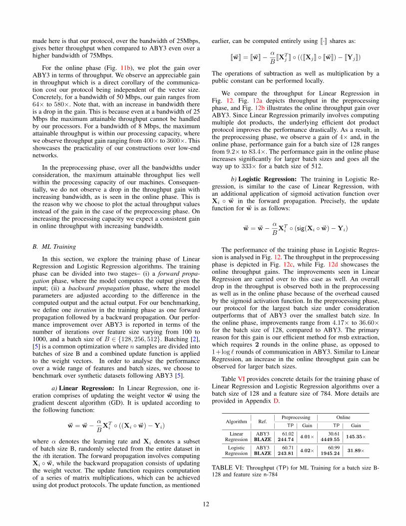
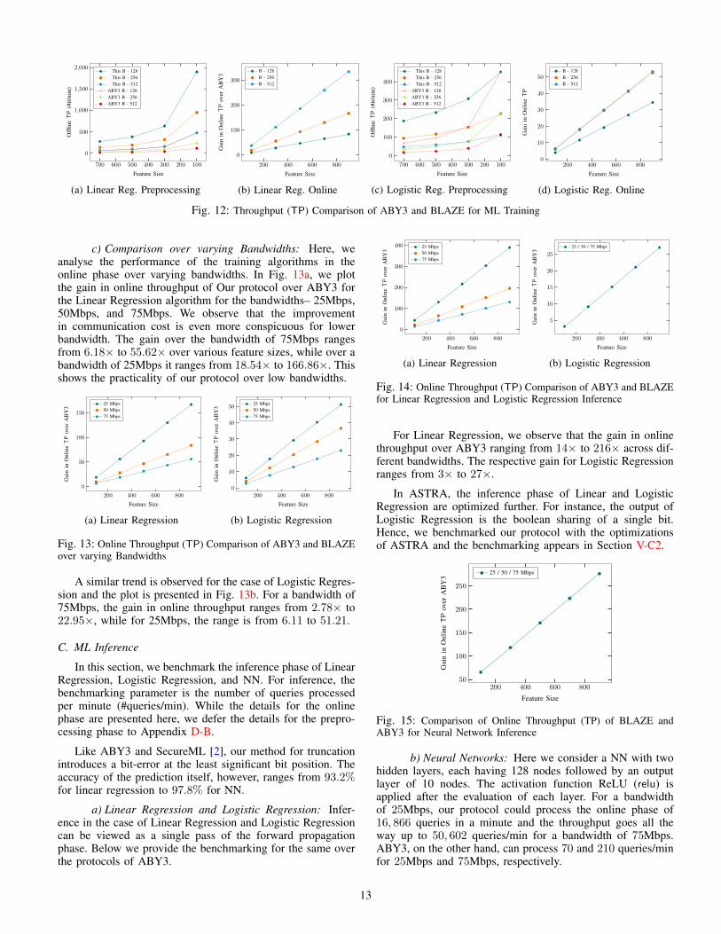
We compare the throughput for Linear Regression inFig. 12. Fig. 12a depicts throughput in the preprocessingphase, and Fig. 12b illustrates the online throughput gain overABY3. Since Linear Regression primarily involves computingmultiple dot products, the underlying efficient dot productprotocol improves the performance drastically. As a result, inthe preprocessing phase, we observe a gain of 4× and, in theonline phase, performance gain for a batch size of 128 rangesfrom 9.2× to 83.4×. The performance gain in the online phaseincreases significantly for larger batch sizes and goes all theway up to 333× for a batch size of 512.

b) Logistic Regression: The training in Logistic Re-gression, is similar to the case of Linear Regression, withan additional application of sigmoid activation function overXi ◦ ~w in the forward propagation. Precisely, the updatefunction for ~w is as follows:

~w = ~w − α

BXTi ◦ (sig(Xi ◦ ~w)−Yi)

The performance of the training phase in Logistic Regres-sion is analysed in Fig. 12. The throughput in the preprocessingphase is depicted in Fig. 12c, while Fig. 12d showcases theonline throughput gains. The improvements seen in LinearRegression are carried over to this case as well. An overalldrop in the throughput is observed both in the preprocessingas well as in the online phase because of the overhead causedby the sigmoid activation function. In the preprocessing phase,our protocol for the largest batch size under considerationoutperforms that of ABY3 over the smallest batch size. Inthe online phase, improvements range from 4.17× to 36.60×for the batch size of 128, compared to ABY3. The primaryreason for this gain is our efficient method for msb extraction,which requires 2 rounds in the online phase, as opposed to1+log ` rounds of communication in ABY3. Similar to LinearRegression, an increase in the online throughput gain can beobserved for larger batch sizes.

Table VI provides concrete details for the training phase ofLinear Regression and Logistic Regression algorithms over abatch size of 128 and a feature size of 784. More details areprovided in Appendix D.

Algorithm Ref.Preprocessing Online

TP Gain TP Gain

LinearRegression

ABY3 61.024.01× 30.61

145.35×BLAZE 244.74 4449.55

LogisticRegression

ABY3 60.714.02× 60.99

31.89×BLAZE 243.81 1945.24

TABLE VI: Throughput (TP) for ML Training for a batch size B-128 and feature size n-784

12

100200300400500600700

0

500

1,000

1,500

2,000

Feature Size

Offl

ine

TP

(#it/

min

)This B - 128This B - 256This B - 512

ABY3 B - 128ABY3 B - 256ABY3 B - 512

(a) Linear Reg. Preprocessing

200 400 600 800

0

100

200

300

Feature Size

Gai

nin

Onl

ine

TP

over

AB

Y3

B - 128B - 256B - 512

(b) Linear Reg. Online

100200300400500600700

0

100

200

300

400

Feature Size

Offl

ine

TP

(#it/

min

)

This B - 128This B - 256This B - 512

ABY3 B - 128ABY3 B - 256ABY3 B - 512

(c) Logistic Reg. Preprocessing

200 400 600 8000

10

20

30

40

50

Feature Size

Gai

nin

Onl

ine

TP

B - 128B - 256B - 512

(d) Logistic Reg. Online

Fig. 12: Throughput (TP) Comparison of ABY3 and BLAZE for ML Training

c) Comparison over varying Bandwidths: Here, weanalyse the performance of the training algorithms in theonline phase over varying bandwidths. In Fig. 13a, we plotthe gain in online throughput of Our protocol over ABY3 forthe Linear Regression algorithm for the bandwidths– 25Mbps,50Mbps, and 75Mbps. We observe that the improvementin communication cost is even more conspicuous for lowerbandwidth. The gain over the bandwidth of 75Mbps rangesfrom 6.18× to 55.62× over various feature sizes, while over abandwidth of 25Mbps it ranges from 18.54× to 166.86×. Thisshows the practicality of our protocol over low bandwidths.

200 400 600 800

0

50

100

150

Feature Size

Gai

nin

Onl

ine

TP

over

AB

Y3

25 Mbps50 Mbps75 Mbps

(a) Linear Regression

200 400 600 800

0

10

20

30

40

50

Feature Size

Gai

nin

Onl

ine

TP

over

AB

Y3

25 Mbps50 Mbps75 Mbps

(b) Logistic Regression

Fig. 13: Online Throughput (TP) Comparison of ABY3 and BLAZEover varying Bandwidths

A similar trend is observed for the case of Logistic Regres-sion and the plot is presented in Fig. 13b. For a bandwidth of75Mbps, the gain in online throughput ranges from 2.78× to22.95×, while for 25Mbps, the range is from 6.11 to 51.21.

C. ML Inference

In this section, we benchmark the inference phase of LinearRegression, Logistic Regression, and NN. For inference, thebenchmarking parameter is the number of queries processedper minute (#queries/min). While the details for the onlinephase are presented here, we defer the details for the prepro-cessing phase to Appendix D-B.

Like ABY3 and SecureML [2], our method for truncationintroduces a bit-error at the least significant bit position. Theaccuracy of the prediction itself, however, ranges from 93.2%for linear regression to 97.8% for NN.

a) Linear Regression and Logistic Regression: Infer-ence in the case of Linear Regression and Logistic Regressioncan be viewed as a single pass of the forward propagationphase. Below we provide the benchmarking for the same overthe protocols of ABY3.

200 400 600 800

0

100

200

300

400

Feature Size

Gai

nin

Onl

ine

TP

over

AB

Y3

25 Mbps50 Mbps75 Mbps

(a) Linear Regression

200 400 600 800

5

10

15

20

25

Feature Size

Gai

nin

Onl

ine

TP

over

AB

Y3

25 / 50 / 75 Mbps

(b) Logistic Regression

Fig. 14: Online Throughput (TP) Comparison of ABY3 and BLAZEfor Linear Regression and Logistic Regression Inference

For Linear Regression, we observe that the gain in onlinethroughput over ABY3 ranging from 14× to 216× across dif-ferent bandwidths. The respective gain for Logistic Regressionranges from 3× to 27×.

In ASTRA, the inference phase of Linear and LogisticRegression are optimized further. For instance, the output ofLogistic Regression is the boolean sharing of a single bit.Hence, we benchmarked our protocol with the optimizationsof ASTRA and the benchmarking appears in Section V-C2.

200 400 600 80050

100

150

200

250

Feature Size

Gai

nin

Onl

ine

TP

over

AB

Y3

25 / 50 / 75 Mbps

Fig. 15: Comparison of Online Throughput (TP) of BLAZE andABY3 for Neural Network Inference

b) Neural Networks: Here we consider a NN with twohidden layers, each having 128 nodes followed by an outputlayer of 10 nodes. The activation function ReLU (relu) isapplied after the evaluation of each layer. For a bandwidthof 25Mbps, our protocol could process the online phase of16, 866 queries in a minute and the throughput goes all theway up to 50, 602 queries/min for a bandwidth of 75Mbps.ABY3, on the other hand, can process 70 and 210 queries/minfor 25Mbps and 75Mbps, respectively.

13

Fig. 15 plots the gain in online throughput of BLAZE overABY3 for varying feature sizes. Unlike Linear Regressionand Logistic Regression, the gain is not dropped with theincrease in bandwidth. This is because of the huge communi-cation incurred for NN which makes the maximum attainablethroughput within our processing capacity.

Table VII provides concrete details for the inference phaseof the aforementioned algorithms for feature size of 784.

Algorithm Ref.Preprocessing Online

TP (×103) Gain TP (×103) Gain

LinearRegression

ABY3 15.574.02× 15.67

169.75×BLAZE 62.61 2660.53

LogisticRegression

ABY3 15.414.03× 15.55

23.57×BLAZE 62.13 366.68

NeuralNetworks

ABY3 0.104.01× 0.14

245.74×BLAZE 0.41 33.74

TABLE VII: Throughput (TP) for ML Inference for a feature sizeof n-784

1) ML Inference on Real World Datasets: Here we bench-mark the online phase of ML inference of all the threealgorithms over real-world datasets (Table IX). The datasetsare obtained from UCI Machine Learning Repository [50] andthe details are provided in Table VIII.

Algorithm Dataset #features #samples

LinearRegression

Superconductivity CriticalTemperature Data Set [51] 81 21263

LogisticRegression

FMA Music AnalysisDataset [52] 518 106574

NeuralNetworks

Parkinson DiseaseClassification Dataset [53] 754 754

TABLE VIII: Real World Datasets used for ML Inference

BandwidthLinear Regression Logistic Regression Neural Networks

(Superconductivity) (FMA) (Parkinson)ABY3 BLAZE ABY3 BLAZE ABY3 BLAZE

25 Mbps 75852 2660532 11725 183339 70 1686750 Mbps 151704 2660532 23450 366678 140 3373575 Mbps 227556 2660532 35175 550017 210 50603

TABLE IX: Comparison of Online TP of ABY3 and BLAZE forInference over Real World Datasets (Datasets are given in Brackets).Values are given in #queries/min.

In Table IX, we observe that the online throughput of ourprotocols for the case of Linear Regression is not increasingwith the increase in bandwidth. This can be justified as theprocessing capacity becomes the bottleneck and prevents ourprotocols from reaching the maximum attainable throughputeven for a bandwidth of 25Mbps. This can be prevented byintroducing more computing power to the environment.

2) Comparison with ASTRA: Here we compare LinearRegression and Logistic Regression inference of BLAZE andASTRA. For a fair comparison, we apply the optimizationsproposed by ASTRA in our protocols. Since Linear Regressioninference essentially reduces to a dot product, the benchmark-ing for the former can be used to analyse the performance of

dot product of BLAZE and ASTRA. Hence we omit a separatebenchmarking for dot product.

In Fig. 16, we plot the online throughput of BLAZEand ASTRA for Linear Regression (Fig. 16a) and LogisticRegression (Fig. 16b) inference. Concretely, we plot the gainin online throughput over ASTRA over different batch sizesand bandwidths. For the preprocessing phase, our protocolsclearly outperforms that of ASTRA and hence we omit theplot for the same.

200 400 600 800

0

50

100

150

200

Feature Size

Gai

nin

Onl

ine

TP

over

AST

RA 25 Mbps

50 Mbps75 Mbps

(a) Linear Regression Inference

200 400 600 800

5

10

15

Feature Size

Gai

nin

Onl

ine

TP

over

AST

RA 25 / 50 / 75 Mbps

(b) Logistic Regression Inference

Fig. 16: Online Throughput (TP) Comparison of ASTRA andBLAZE for Linear Regression and Logistic Regression Inference

For both Linear Regression and Logistic Regression in-ference, we observe that the gain in online throughput overASTRA drops with an increase in bandwidth. This is becauseof our limited processing capacity which prevents our protocolsfrom attaining the maximum attainable throughput even for abandwidth of 25 Mbps. On the other hand, the throughput ofASTRA increases with the increase in bandwidth. To see this,we limited the bandwidth further to 3Mbps. At 3Mbps, thegain in online throughput over ASTRA ranges from 180× to1623× for Linear Regression inference.

VI. CONCLUSION

In this work, we presented a blazing fast framework,BLAZE, for PPML. Our framework, designed for three serverstolerating at most one malicious corruption, works seamlesslyover a ring Z2` . Cast in the preprocessing model, our constructs

14

outperform the state-of-the-art solutions by several orders ofmagnitude both in the round and communication complexity.We showcased the application of our framework in LinearRegression, Logistic Regression, and Neural Networks. Weleave open the problem of extending our framework to supporttraining of Neural Networks. Another interesting line of workis to explore the potential of Trusted Execution Environments(TEE) [4] in improving the overall efficiency of the frame-work.

ACKNOWLEDGEMENT

We thank our shepherd Matt Fredrikson, and anonymousreviewers for their valuable feedback.

REFERENCES

[1] A. Madani, R. Arnaout, M. R. K. Mofrad, and R. Arnaout, “Fast andaccurate classification of echocardiograms using deep learning,” npjDigital Medicine, 2018.

[2] P. Mohassel and Y. Zhang, “Secureml: A system for scalable privacy-preserving machine learning,” in IEEE S&P, 2017, pp. 19–38.

[3] E. Makri, D. Rotaru, N. P. Smart, and F. Vercauteren, “EPIC: efficientprivate image classification (or: Learning from the masters),” in CT-RSA, 2019, pp. 473–492.

[4] M. S. Riazi, C. Weinert, O. Tkachenko, E. M. Songhori, T. Schneider,and F. Koushanfar, “Chameleon: A hybrid secure computation frame-work for machine learning applications,” in AsiaCCS, 2018, pp. 707–721.

[5] P. Mohassel and P. Rindal, “ABY3: A mixed protocol framework formachine learning,” in ACM CCS, 2018, pp. 35–52.

[6] S. Wagh, D. Gupta, and N. Chandran, “Securenn: 3-party securecomputation for neural network training,” PoPETs, pp. 26–49, 2019.

[7] T. Araki, J. Furukawa, Y. Lindell, A. Nof, and K. Ohara, “High-throughput semi-honest secure three-party computation with an honestmajority,” in ACM CCS, 2016, pp. 805–817.

[8] J. Furukawa, Y. Lindell, A. Nof, and O. Weinstein, “High-throughputsecure three-party computation for malicious adversaries and an honestmajority,” in EUROCRYPT, 2017, pp. 225–255.

[9] T. Araki, A. Barak, J. Furukawa, T. Lichter, Y. Lindell, A. Nof,K. Ohara, A. Watzman, and O. Weinstein, “Optimized honest-majorityMPC for malicious adversaries - breaking the 1 billion-gate per secondbarrier,” in IEEE S&P, 2017, pp. 843–862.

[10] Y. Lindell and A. Nof, “A framework for constructing fast MPC overarithmetic circuits with malicious adversaries and an honest-majority,”in ACM CCS, 2017, pp. 259–276.

[11] K. Chida, D. Genkin, K. Hamada, D. Ikarashi, R. Kikuchi, Y. Lindell,and A. Nof, “Fast large-scale honest-majority MPC for maliciousadversaries,” in CRYPTO, 2018, pp. 34–64.

[12] P. Mohassel, M. Rosulek, and Y. Zhang, “Fast and secure three-partycomputation: The garbled circuit approach,” in ACM CCS, 2015, pp.591–602.

[13] Y. Ishai, R. Kumaresan, E. Kushilevitz, and A. Paskin-Cherniavsky,“Secure computation with minimal interaction, revisited,” in CRYPTO,2015, pp. 359–378.

[14] A. Patra and D. Ravi, “On the exact round complexity of secure three-party computation,” in CRYPTO, 2018, pp. 425–458.

[15] M. Byali, A. Joseph, A. Patra, and D. Ravi, “Fast secure computationfor small population over the internet,” in ACM CCS, 2018, pp. 677–694.

[16] P. S. Nordholt and M. Veeningen, “Minimising communication inhonest-majority MPC by batchwise multiplication verification,” inACNS, 2018, pp. 321–339.

[17] D. Boneh, E. Boyle, H. Corrigan-Gibbs, N. Gilboa, and Y. Ishai,“Zero-knowledge proofs on secret-shared data via fully linear pcps,”in CRYPTO, 2019, pp. 67–97.

[18] D. Bogdanov, R. Talviste, and J. Willemson, “Deploying secure multi-party computation for financial data analysis - (short paper),” in FC,2012, pp. 57–64.

[19] J. Launchbury, D. Archer, T. DuBuisson, and E. Mertens, “Application-scale secure multiparty computation,” in ESOP, 2014, pp. 8–26.

[20] D. Bogdanov, L. Kamm, B. Kubo, R. Rebane, V. Sokk, and R. Talviste,“Students and taxes: a privacy-preserving social study using securecomputation,” PoPETs, pp. 117–135, 2016.

[21] D. Bogdanov, S. Laur, and J. Willemson, “Sharemind: A framework forfast privacy-preserving computations,” in ESORICS, 2008, pp. 192–206.

[22] M. Geisler, “Viff: Virtual ideal functionality framework,” 2007.[23] D. Beaver, “Efficient multiparty protocols using circuit randomization,”

in CRYPTO, 1991, pp. 420–432.[24] ——, “Precomputing oblivious transfer,” in CRYPTO, 1995, pp. 97–

109.[25] Z. Beerliova-Trubıniova and M. Hirt, “Efficient multi-party computation

with dispute control,” in TCC, 2006, pp. 305–328.[26] ——, “Perfectly-secure MPC with linear communication complexity,”

in TCC, 2008, pp. 213–230.[27] E. Ben-Sasson, S. Fehr, and R. Ostrovsky, “Near-linear unconditionally-

secure multiparty computation with a dishonest minority,” in CRYPTO,2012, pp. 663–680.

[28] A. Choudhury and A. Patra, “An efficient framework for uncondition-ally secure multiparty computation,” IEEE Trans. Information Theory,vol. 63, no. 1, pp. 428–468, 2017.

[29] I. Damgard, V. Pastro, N. P. Smart, and S. Zakarias, “Multipartycomputation from somewhat homomorphic encryption,” in CRYPTO,2012, pp. 643–662.

[30] I. Damgard, M. Keller, E. Larraia, V. Pastro, P. Scholl, and N. P. Smart,“Practical covertly secure MPC for dishonest majority - or: Breakingthe SPDZ limits,” in ESORICS, 2013, pp. 1–18.

[31] M. Keller, P. Scholl, and N. P. Smart, “An architecture for practicalactively secure MPC with dishonest majority,” in ACM CCS, 2013, pp.549–560.

[32] M. Keller, E. Orsini, and P. Scholl, “MASCOT: faster maliciousarithmetic secure computation with oblivious transfer,” in ACM CCS,2016, pp. 830–842.

[33] C. Baum, I. Damgard, T. Toft, and R. W. Zakarias, “Better preprocessingfor secure multiparty computation,” in ACNS, 2016, pp. 327–345.

[34] I. Damgard, C. Orlandi, and M. Simkin, “Yet another compiler for activesecurity or: Efficient MPC over arbitrary rings,” in CRYPTO, 2018, pp.799–829.

[35] R. Cramer, I. Damgard, D. Escudero, P. Scholl, and C. Xing, “SPDZ2k :Efficient MPC mod 2k for Dishonest Majority,” in CRYPTO, 2018, pp.769–798.

[36] M. Keller, V. Pastro, and D. Rotaru, “Overdrive: Making SPDZ greatagain,” in EUROCRYPT, 2018, pp. 158–189.

[37] R. Cramer, S. Fehr, Y. Ishai, and E. Kushilevitz, “Efficient multi-partycomputation over rings,” in EUROCRYPT, 2003, pp. 596–613.

[38] D. Demmler, T. Schneider, and M. Zohner, “ABY - A framework forefficient mixed-protocol secure two-party computation,” in NDSS, 2015.

[39] I. Damgard, D. Escudero, T. K. Frederiksen, M. Keller, P. Scholl, andN. Volgushev, “New primitives for actively-secure MPC over rings withapplications to private machine learning,” IEEE S&P, pp. 1102–1120,2019.

[40] Y. Lindell and B. Pinkas, “Privacy preserving data mining,” in CRYPTO,2000, pp. 36–54.

[41] W. Du and M. J. Atallah, “Privacy-preserving cooperative scientificcomputations,” in IEEE (CSFW-14, 2001, pp. 273–294.

[42] A. P. Sanil, A. F. Karr, X. Lin, and J. P. Reiter, “Privacy preservingregression modelling via distributed computation,” in ACM SIGKDD,2004, pp. 677–682.

[43] G. Jagannathan and R. N. Wright, “Privacy-preserving distributed k-means clustering over arbitrarily partitioned data,” in ACM SIGKDD,2005, pp. 593–599.

[44] P. Bunn and R. Ostrovsky, “Secure two-party k-means clustering,” inACM CCS, 2007, pp. 486–497.

15

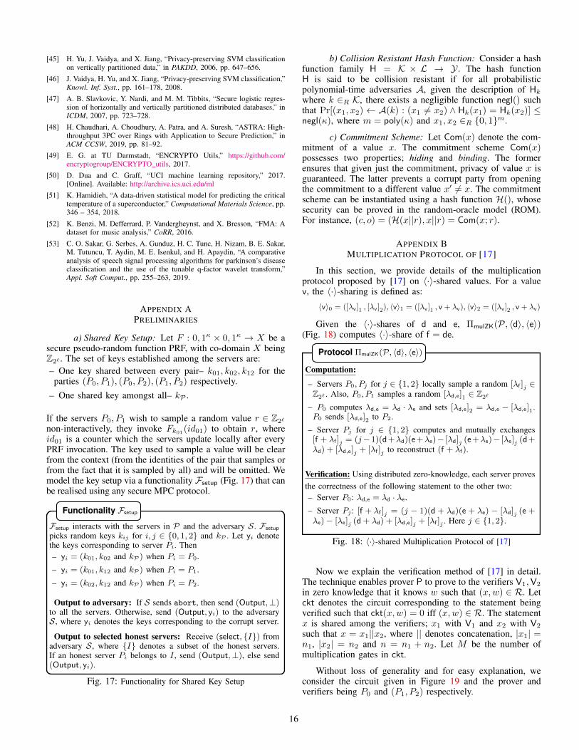
[45] H. Yu, J. Vaidya, and X. Jiang, “Privacy-preserving SVM classificationon vertically partitioned data,” in PAKDD, 2006, pp. 647–656.

[46] J. Vaidya, H. Yu, and X. Jiang, “Privacy-preserving SVM classification,”Knowl. Inf. Syst., pp. 161–178, 2008.

[47] A. B. Slavkovic, Y. Nardi, and M. M. Tibbits, “Secure logistic regres-sion of horizontally and vertically partitioned distributed databases,” inICDM, 2007, pp. 723–728.

[48] H. Chaudhari, A. Choudhury, A. Patra, and A. Suresh, “ASTRA: High-throughput 3PC over Rings with Application to Secure Prediction,” inACM CCSW, 2019, pp. 81–92.

[49] E. G. at TU Darmstadt, “ENCRYPTO Utils,” https://github.com/encryptogroup/ENCRYPTO utils, 2017.

[50] D. Dua and C. Graff, “UCI machine learning repository,” 2017.[Online]. Available: http://archive.ics.uci.edu/ml

[51] K. Hamidieh, “A data-driven statistical model for predicting the criticaltemperature of a superconductor,” Computational Materials Science, pp.346 – 354, 2018.

[52] K. Benzi, M. Defferrard, P. Vandergheynst, and X. Bresson, “FMA: Adataset for music analysis,” CoRR, 2016.

[53] C. O. Sakar, G. Serbes, A. Gunduz, H. C. Tunc, H. Nizam, B. E. Sakar,M. Tutuncu, T. Aydin, M. E. Isenkul, and H. Apaydin, “A comparativeanalysis of speech signal processing algorithms for parkinson’s diseaseclassification and the use of the tunable q-factor wavelet transform,”Appl. Soft Comput., pp. 255–263, 2019.

APPENDIX APRELIMINARIES

a) Shared Key Setup: Let F : 0, 1κ × 0, 1κ → X be asecure pseudo-random function PRF, with co-domain X beingZ2` . The set of keys established among the servers are:– One key shared between every pair– k01, k02, k12 for the

parties (P0, P1), (P0, P2), (P1, P2) respectively.– One shared key amongst all– kP .

If the servers P0, P1 wish to sample a random value r ∈ Z2`

non-interactively, they invoke Fk01(id01) to obtain r, whereid01 is a counter which the servers update locally after everyPRF invocation. The key used to sample a value will be clearfrom the context (from the identities of the pair that samples orfrom the fact that it is sampled by all) and will be omitted. Wemodel the key setup via a functionality Fsetup (Fig. 17) that canbe realised using any secure MPC protocol.

Fsetup interacts with the servers in P and the adversary S. Fsetup

picks random keys kij for i, j ∈ {0, 1, 2} and kP . Let yi denotethe keys corresponding to server Pi. Then– yi = (k01, k02 and kP) when Pi = P0.

– yi = (k01, k12 and kP) when Pi = P1.

– yi = (k02, k12 and kP) when Pi = P2.

Output to adversary: If S sends abort, then send (Output,⊥)to all the servers. Otherwise, send (Output, yi) to the adversaryS, where yi denotes the keys corresponding to the corrupt server.

Output to selected honest servers: Receive (select, {I}) fromadversary S, where {I} denotes a subset of the honest servers.If an honest server Pi belongs to I , send (Output,⊥), else send(Output, yi).

Functionality Fsetup

Fig. 17: Functionality for Shared Key Setup

b) Collision Resistant Hash Function: Consider a hashfunction family H = K × L → Y . The hash functionH is said to be collision resistant if for all probabilisticpolynomial-time adversaries A, given the description of Hkwhere k ∈R K, there exists a negligible function negl() suchthat Pr[(x1, x2) ← A(k) : (x1 6= x2) ∧ Hk(x1) = Hk(x2)] ≤negl(κ), where m = poly(κ) and x1, x2 ∈R {0, 1}m.

c) Commitment Scheme: Let Com(x) denote the com-mitment of a value x. The commitment scheme Com(x)possesses two properties; hiding and binding. The formerensures that given just the commitment, privacy of value x isguaranteed. The latter prevents a corrupt party from openingthe commitment to a different value x′ 6= x. The commitmentscheme can be instantiated using a hash function H(), whosesecurity can be proved in the random-oracle model (ROM).For instance, (c, o) = (H(x||r), x||r) = Com(x; r).

APPENDIX BMULTIPLICATION PROTOCOL OF [17]

In this section, we provide details of the multiplicationprotocol proposed by [17] on 〈·〉-shared values. For a valuev, the 〈·〉-sharing is defined as:

〈v〉0 = ([λv]1 , [λv]2), 〈v〉1 = ([λv]1 , v + λv), 〈v〉2 = ([λv]2 , v + λv)

Given the 〈·〉-shares of d and e, ΠmulZK(P, 〈d〉, 〈e〉)(Fig. 18) computes 〈·〉-share of f = de.

Computation:

– Servers P0, Pj for j ∈ {1, 2} locally sample a random [λf ]j ∈Z2` . Also, P0, P1 samples a random [λd,e]1 ∈ Z2`

– P0 computes λd,e = λd · λe and sets [λd,e]2 = λd,e − [λd,e]1.P0 sends [λd,e]2 to P2.

– Server Pj for j ∈ {1, 2} computes and mutually exchanges[f + λf ]j = (j−1)(d +λd)(e +λe)− [λd]j (e +λe)− [λe]j (d +λd) + [λd,e]j + [λf ]j to reconstruct (f + λf).

Verification: Using distributed zero-knowledge, each server provesthe correctness of the following statement to the other two:– Server P0: λd,e = λd · λe.

– Server Pj : [f + λf ]j = (j − 1)(d + λd)(e + λe) − [λd]j (e +λe)− [λe]j (d + λd) + [λd,e]j + [λf ]j . Here j ∈ {1, 2}.

Protocol ΠmulZK(P, 〈d〉, 〈e〉)

Fig. 18: 〈·〉-shared Multiplication Protocol of [17]

Now we explain the verification method of [17] in detail.The technique enables prover P to prove to the verifiers V1,V2

in zero knowledge that it knows w such that (x,w) ∈ R. Letckt denotes the circuit corresponding to the statement beingverified such that ckt(x,w) = 0 iff (x,w) ∈ R. The statementx is shared among the verifiers; x1 with V1 and x2 with V2

such that x = x1||x2, where || denotes concatenation, |x1| =n1, |x2| = n2 and n = n1 + n2. Let M be the number ofmultiplication gates in ckt.

Without loss of generality and for easy explanation, weconsider the circuit given in Figure 19 and the prover andverifiers being P0 and (P1, P2) respectively.

16

×

+

×

v1

v2

x1

x2

7

w

v3

Fig. 19: Example circuit

The prover P0 first constructs three polynomials f(),g() and h() on the values on left, right and output wires,respectively, of the multiplication gates. The constant termsof f() and g() are set as random ring elements z1 and z2respectively, while the constant term for h() is set as z1z2.More precisely,

f(0) = z1, g(0) = z2, h(0) = z1z2f(1) = x2, g(1) = x1, h(1) = x1x2f(2) = v2 = 7 + w, g(2) = v1 = x1x2, h(2) = v1v2

With the above values set, P0 interpolates the polynomialsf(), g() and h(). While f(), g() are polynomials of degreeat most M , h() is a polynomial of degree at most d = 2M .The proof π is then defined as (w, z1, z2, ch) ∈ Zσ2` where chdenotes the coefficients of h(). The size of proof is denotedby σ = s+ d+ 3 where s is the size of the witness. P0 thenprovides additive shares of π, denoted by πi, to the verifiers;πi to Pi for i ∈ {1, 2}. Note that if P0 is honest then ∀r ∈Z2` , h(r) = f(r)g(r) and h(M) = 0.

Verifiers P1, P2 together sample a random value r ∈Z2` \{z1, z2} and generate corresponding query vectors qf , qgand qh ∈ Zn+σ

2`. Each verifier Pi for i ∈ {1, 2} then construct

three query vectors from qf , qg and qh. More precisely,corresponding to polynomial f(), verifier Pi constructs vectorQif ∈ Fni+σ from qf such that the first ni positions arereserved for entries corresponding to xi followed by qf . Pifor i ∈ {1, 2} then locally computes the dot product (�) ofthe vectors (xi||πi) and Qif as fi(r) = (xi||πi)�Qif and sendsit to verifier P1. P1 after receiving the shares of fi(r) computesthe value f(r) = f1(r) + f2(r). This comes from the fact thateach query vector q defines a linear combination of the inputx and proof π. Hence, the verifiers can form additive shares ofthe answers to the queries, which is the polynomials evaluatedat r, using their parts of input xi and additive share πi. Thiscomes from the fact that each query vector q defines a linearcombination of the input x and proof π. Hence, the verifierscan form additive shares of the answers to the queries, whichis the polynomials evaluated at r, using their parts of input xiand additive share πi. Similar steps are done for polynomialsg() and h() which enables P1 to obtain g(r) and h(r). P1

aborts if h(r) 6= f(r)g(r). A cheating prover P0 will passthis check with probability at most 2M−1

2`−2 , which for a largeenough ` is negligible.

Now for the second check, ie. h(M) = 0, verifiers generatequery vector q in a similar fashion. More precisely, Pi for i ∈{1, 2} forms Qi, computes hi(M) and sends his share of h(M)to P1. Verifier P1 abort if h(M) 6= h1(M) + h2(M) = 0.

[17] propose two variants of the above technique. The firstvariant gives a 2 round fully linear interactive oracle proofswith query complexity O (

√n), where n is the size of the

input. The second variant gives O (log(M)) rounds fully linearinteractive oracle proofs with query complexity of O (log(M)),where M is the number of multiplication gates in ckt. Weuse the former result in our work. We refer the readers to[17] for a more detailed description of the verification and itsoptimizations.

Lemma B.1 (Communication). Protocol ΠmulZK requires 4rounds and an amortized communication of 3` bits.

The ideal-world functionality realising ΠmulZK protocol ispresented in Fig. 20.

FmulZK interacts with the servers in P and the adversary S. FmulZK

receives the 〈·〉-shares of values d and e from the servers where,

〈d〉0 = ([λd]1 , [λd]2), 〈d〉1 = ([λd]1 , d + λd), 〈d〉2 = ([λd]2 , d + λd)〈e〉0 = ([λe]1 , [λe]2), 〈e〉1 = ([λe]1 , e + λe), 〈e〉2 = ([λe]2 , e + λe)

If the functionality receives ⊥ from S, then send ⊥ to everyserver, else do the following:

Computation of output: Compute d = (d +λd)− [λd]1− [λd]2and e = (e + λe) − [λe]1 − [λe]2 followed by computing f = de.Randomly select [λf ]1 , [λf ]2 from Z2` and set λf = [λf ]1 + [λf ]2.The output shares are set as

〈f〉0 = ([λf ]1 , [λf ]2), 〈f〉1 = ([λf ]1 , f + λf), 〈f〉2 = ([λf ]2 , f + λf)

Output to adversary: If S sends abort, then send (Output,⊥)to all the servers. Otherwise, send (Output, 〈f〉S) to the adversaryS, where 〈f〉S denotes the share of f corresponding to the corruptserver.

Output to selected honest servers: Receive (select, {I}) fromadversary S, where {I} denotes a subset of the honest servers.If an honest server Pi belongs to I , send (Output,⊥), else send(Output, 〈f〉i), where 〈f〉i denotes the share of f corresponding tothe honest server Pi.

Functionality FmulZK

Fig. 20: Functionality for ΠmulZK

APPENDIX CBUILDING BLOCKS

A. Secret Sharing and Reconstruction Protocols

1) Sharing Protocol:

Lemma C.1 (Communication). Protocol Πsh (Fig. 2) is non-interactive in the preprocessing phase and requires 1 roundand an amortized communication of 2` bits in the online phase.

Proof: During the preprocessing phase, servers sample theshares of α and γ values non-interactively using the sharedkey setup. During the online phase, when Pi = P0, he/shecomputes and sends β to both P1 and P2 resulting in 1 roundand a communication of 2` ring elements. This is followedby P1, P2 mutually exchanging hash of β value received fromP0. Servers can combine β-values for several instances into asingle hash and hence the cost gets amortized over multipleinstances. For the case when Pi = P1, she sends β and

17

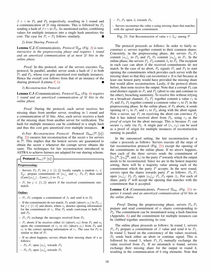
β + γ to P2 and P0 respectively, resulting in 1 round anda communication of 2` ring elements. This is followed by P2

sending a hash of β+γ to P0. As mentioned earlier, combiningvalues for multiple instances into a single hash amortizes thecost. The case for Pi = P2 follows similarly.

2) Joint Sharing Protocol:

Lemma C.2 (Communication). Protocol Πjsh (Fig. 3) is non-interactive in the preprocessing phase and requires 1 roundand an amortized communication of at most 2` bits in theonline phase.

Proof: In this protocol, one of the servers executes Πsh

protocol. In parallel, another server sends a hash of β to bothP1 and P2, whose cost gets amortized over multiple instances.Hence the overall cost follows from that of an instance of thesharing protocol (Lemma C.1).

3) Reconstruction Protocol:

Lemma C.3 (Communication). Protocol Πrec (Fig. 4) requires1 round and an amortized communication of 3` bits in theonline phase.

Proof: During the protocol, each server receives hermissing share from another server, resulting in 1 round anda communication of 3` bits. Also, each server receives a hashof the missing share from another server for verification. Thehash for multiple instances can be combined to a single hashand thus this cost gets amortized over multiple instances.

4) Fair Reconstruction Protocol: Protocol Πfrec(P, JvK)(Fig. 21) ensures fair reconstruction of the secret v for serversin P . This implies that the honest servers are guaranteed toobtain the secret v whenever the corrupt server obtains thesame. The techniques for fair reconstruction introduced inASTRA to achieve fairness are adapted for our sharing scheme.

Preprocessing:

– Servers P0, Pj for j ∈ {1, 2} locally sample a random rj ∈Z2` , prepare commitments of [αv]j and rj . P0, Pj then send(Com([αv]j) , Com(rj)) to P2−j .

– Pj for j ∈ {1, 2} abort if the received commitments mis-match.

Online:

– P1, P2 compute a commitment of βv and send it to P0.

– If the commitments do not match, P0 sends (abort, oj) to P2−j

for j ∈ {1, 2} and aborts, where oj denotes opening informationfor the commitment of rj . Else P0 sends continue to both P1

and P2.

– P1, P2 exchange the messages received from P0.

– P1 aborts if he receives either (i) (abort, o2) from P0 and o2opens the commitment of r2 or (ii) (abort, o1) from P2 ando1 is the correct opening information of r1. The case for P2 issimilar to that of P1

– If no abort happens, servers obtain their missing share of v asfollows:– P0, P1 open [αv]1 towards P2.

– P0, P2 open [αv]2 towards P1.

Protocol Πfrec(P, JvK)

– P1, P2 open βv towards P0.

– Servers reconstruct the value v using missing share that matcheswith the agreed upon commitment.

Fig. 21: Fair Reconstruction of value v ∈ Z2` among P

The protocol proceeds as follows: In order to fairly re-construct v, servers together commit to their common shares.Concretely, in the preprocessing phase, the servers P0, P1

commit [αv]1 to P2 and P0, P2 commit [αv]2 to P1. In theonline phase, the servers P1, P2 commit βv to P0. The recipientin each case can abort if the received commitments do notmatch. In the case of no abort, P0 signals P1 and P2 to startopening the commitments which provides each server with themissing share so that they can reconstruct v. It is fair because atleast one honest party would have provided the missing sharethat would allow reconstruction. Lastly, if the protocol abortsbefore, then none receive the output. Note that a corrupt P0 cansend distinct signals to P1 and P2 (abort to one and continue tothe other), breaching unanimity. To resolve this without relyingon a broadcast channel, P0, P1 together commit a value r1 toP2 and P0, P2 together commit a common value r2 to P1 in thepreprocessing phase. In the online phase, if P0 aborts, it sendsopening of r2 to P1 and r1 to P2, along with the abort signal.Now a server, say P1 on receiving the abort can convince P2

that it has indeed received abort from P0, using r2 as theproof of origin for the abort message. This is because P1 cansecure r2 only via P0. A single pair of (r1, r2) can be usedas a proof of origin for multiple instances of reconstructionrunning in parallel.

In the outsourced setting, the fair reconstruction of avalue v proceeds as follows: Servers execute all the steps offair reconstruction protocol (Fig. 21) except the opening ofthe commitments in the online phase. If no abort happens,then each of the three servers sends the commitment ofJαvKA, JαvKB, and βv) to the party P towards which the outputneeds to be reconstructed. Since we are in the honest majoritysetting, there will be a majority value among each of thecommitment which the party P accepts. In the next round,servers open the shares towards party P as follows: P0, P1

open [αv]1; P0, P2 open [αv]2; P1, P2 open βv. For each ofshare, party P will accept the opening that matches with thecommitment that it accepted.

Lemma C.4 (Communication). Protocol Πfrec (Fig. 21) re-quires 4 rounds and an amortized communication of 6` bits inthe online phase.

Proof: During the preprocessing phase, servers P0, P1

prepare and send commitment of α shares corresponding toP2. The commitment can be instantiated using a hash function(Appendix A) and the commitment for multiple instances canbe clubbed together amortizing its cost.

The online phase proceeds as follows: In round 1, serversP1, P2 prepare a commitment of β value and send it to P1.In round 2, based on the consistency of the values received,P0 sends back either an abort or continue signal. This isfollowed by round 3, where P1, P2 mutually exchange thevalue received from P0. If no mismatch is found, serversexchange their missing share for the output in round 4,resulting in the communication of 6 ring elements. Note that

18

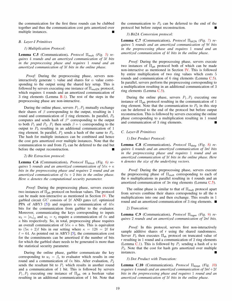
the communication for the first three rounds can be clubbedtogether and thus the communication cost gets amortized overmultiple instances.

B. Layer-I Primitives

1) Multiplication Protocol:

Lemma C.5 (Communication). Protocol Πmult (Fig. 5) re-quires 4 rounds and an amortized communication of 3` bitsin the preprocessing phase and requires 1 round and anamortized communication of 3` bits in the online phase.

Proof: During the preprocessing phase, servers non-interactively generate γ value and shares for α value corre-sponding to the output using the shared key setup. This isfollowed by servers executing one instance of ΠmulZK protocol,which requires 4 rounds and an amortized communication of3 ring elements (Lemma B.1). The rest of the steps in thepreprocessing phase are non-interactive.

During the online phase, servers P1, P2 mutually exchangetheir shares of β corresponding to the output, resulting in 1round and communication of 2 ring elements. In parallel, P0

computes and sends hash of β? corresponding to the outputto both P1 and P2. P1 then sends β + γ corresponding to theoutput to P0 resulting in an additional communication of 1ring element. In parallel, P2 sends a hash of the same to P0.The hash for multiple instances can be combined and hencethe cost gets amortized over multiple instances. Note that thecommunication to and from P0 can be deferred to the end butbefore the output reconstruction.

2) Bit Extraction protocol:

Lemma C.6 (Communication). Protocol Πbitext (Fig. 6) re-quires 5 rounds and an amortized communication of 5`κ+ κbits in the preprocessing phase and requires 2 round and anamortized communication of `κ + 2 bits in the online phase.Here κ denotes the computational security parameter.

Proof: During the preprocessing phase, servers executetwo instances of Πjsh protocol on boolean values. The protocolcan be made non-interactive as mentioned in Section IV. Thegarbled circuit GC consists of 2` AND gates (cf. optimizedPPA of ABY3 [5]) and requires a communication of 4`κbits for the communication from garbler to the evaluator.Moreover, communicating the keys corresponding to inputsu3 = [αv]2 and u5 = r2 require a communication of `κ andκ bits respectively. So, in total, preprocessing phase requiresan overall communication of 5`κ + κ bits. This is equivalentto (5κ + 2)` bits in our setting where κ = 128 = 2` for` = 64. As pointed out in ABY3 [5], the communication costfor the commitments can be amortised if the number of bitsfor which the garbled share needs to be generated is more thanthe statistical security parameter.

During the online phase, garbler communicate the keycorresponding to u1 = βv to evaluator which results in oneround and a communication of `κ bits. After evaluation, P2

sends the resultant bit to P1 which results in another roundand a communication of 1 bit. This is followed by serversP1, P2 executing one instance of Πjsh on a boolean valueresulting in an additional communication of 1 bit. Note that

the communication to P0 can be deferred to the end of theprotocol but before output reconstruction.

3) Bit2A Conversion protocol:

Lemma C.7 (Communication). Protocol Πbit2A (Fig. 7) re-quires 5 rounds and an amortized communication of 9` bitsin the preprocessing phase and requires 1 round and anamortized communication of 4` bits in the online phase.

Proof: During the preprocessing phase, servers executetwo instances of Πjsh protocol both of which can be madenon-interactive as mentioned in Section IV. This is followedby entire multiplication of two ring values which costs 5rounds and communication of 6 ring elements (Lemma C.5).In parallel, servers perform the preprocessing corresponding toa multiplication resulting in an additional communication of 3ring elements (Lemma C.5).

During the online phase, servers P1, P2 executing oneinstance of Πjsh protocol resulting in the communication of 1ring element. Note that the communication to P0 in this stepcan be deferred to the end of the protocol but before outputreconstruction. This is followed by servers executing the onlinephase corresponding to a multiplication resulting in 1 roundand communication of 3 ring elements.

C. Layer-II Primitives

1) Dot Product Protocol:

Lemma C.8 (Communication). Protocol Πdotp (Fig. 8) re-quires 4 rounds and an amortized communication of 3n` bitsin the preprocessing phase and requires 1 round and anamortized communication of 3` bits in the online phase. Heren denotes the size of the underlying vectors.

Proof: During the preprocessing phase, servers executethe preprocessing phase of Πmult corresponding to each ofthe n multiplications in parallel resulting in 4 rounds and anamortized communication of 3n ring elements (Lemma C.5).

The online phase is similar to that of Πmult protocol apartfrom servers combine their shares corresponding to all the nmultiplications into one and then exchange. This results in 1round and an amortized communication of 3 ring elements.

2) Truncation:

Lemma C.9 (Communication). Protocol Πtrgen (Fig. 9) re-quires 2 rounds and an amortized communication of 2n` bits.

Proof: In this protocol, servers first non-interactivelysample additive shares of r using the shared randomness.Server P0 then executes Πsh protocol on truncated value ofr resulting in 1 round and a communication of 2 ring elements(Lemma C.1). This is followed by P1 sending a hash of u toP2. Note that the cost for hash gets amortized over multipleinstances.

3) Dot Product with Truncation:

Lemma C.10 (Communication). Protocol Πdotpt (Fig. 10)requires 4 rounds and an amortized communication of 3n`+2`bits in the preprocessing phase and requires 1 round and anamortized communication of 3` bits in the online phase.

19

Proof: During the preprocessing phase, servers executethe preprocessing phase corresponding to n instances of Πmult

protocol, resulting in a communication of 3n ring elements(Lemma C.8). In parallel, servers execute one instance ofΠtrgen protocol resulting in an additional communication of2 ring elements (Lemma C.9).

The online phase is similar to that of Πdotp protocol apartfrom servers P1, P2 computing additive shares of z− r, wherez = ~x � ~y, which results in a communication of 2 ringelements. This is followed by servers P1, P2 executing oneinstance of Πjsh protocol on the truncated value of z to generateits arithmetic sharing. This incurs a communication of 1 ringelement. This is followed by servers locally adding their shares.Hence, the online phase requires 1 round and an amortizedcommunication of 3 ring elements.

4) Activation Functions:

Lemma C.11 (Communication). Protocol relu requires 5rounds and an amortized communication of 12`+9p bits in thepreprocessing phase and requires 3 rounds and an amortizedcommunication of 7` + 3p + 1 bits in the online phase. Herep denotes the size of the larger field which is p = ` + 25 inthis work.

Proof: One instance of relu protocol involves the execu-tion of one instance of Πbitext, Πbit2A, and Πmult. Hence thecost follows from Lemma C.6, Lemma C.7 and Lemma C.5.

Lemma C.12 (Communication). Protocol sig requires 5rounds and an amortized communication of 21` + 18p + 3bits in the preprocessing phase and requires 4 rounds and anamortized communication of 11` + 6p + 5 bits in the onlinephase.

Proof: One instance of sig protocol involves the executionof the following protocols in order– i) two instances of Πbitext

protocol, ii) once instance of Πmult protocol over booleanvalue, iii) two instances of Πbit2A protocol, and iv) one instanceof Πmult protocol over ring elements. The cost follows fromLemma C.6, Lemma C.7 and Lemma C.5.

APPENDIX DMICRO BENCHMARKING OVER WAN

In this section, we provide detailed benchmarking of MLalgorithms over the WAN setting.

A. ML Training

In Table X, we tabulate the performance in the preprocess-ing phase of the protocol of BLAZE and ABY3 for Linear Re-gression and Logistic Regression Training. The data for batchsize B ∈ {128, 256, 512} and feature sizes {100, 500, 900}are provided. The values in the table shows the number ofiterations in the preprocessing phase that can be completed ina minute. A higher value in the table corresponds a protocolwith lower latency.

Similarly, in Table XI, we tabulate the performance in theonline phase of the protocol of BLAZE and ABY3 for LinearRegression and Logistic Regression Training. The values inthe table shows the number of online iterations that can becompleted in a minute.

Algorithm BatchSize Ref.

Feature Size

n = 100 n = 500 n = 900

LinearRegression

(#iterations/min)

128 ABY3 73.50 68.42 64.72BLAZE 97.08 97.47 91.72

256 ABY3 72.38 64.36 55.96BLAZE 96.60 91.31 84.38

512 ABY3 70.23 55.04 43.30BLAZE 95.65 83.67 70.55

LogisticRegression

(#iterations/min)

128 ABY3 19.77 19.38 19.07BLAZE 31.91 31.51 31.31

256 ABY3 19.68 19.04 18.23BLAZE 31.86 31.26 30.40

512 ABY3 19.52 18.13 16.64BLAZE 31.75 30.31 28.40

TABLE X: Preprocessing Phase: Comparison of ABY3 andBLAZE for ML Training (higher = better)

Algorithm BatchSize Ref.

Feature Size

n = 100 n = 500 n = 900

LinearRegression

(#iterations/min)

128 ABY3 97.57 95.07 89.94BLAZE 139.05 139.05 139.05

256 ABY3 97.11 89.94 80.09BLAZE 139.05 139.05 139.05

512 ABY3 95.08 80.10 68.94BLAZE 139.05 139.05 139.05

LogisticRegression

(#iterations/min)

128 ABY3 20.54 20.43 20.18BLAZE 60.79 60.79 60.79

256 ABY3 20.52 20.18 19.63BLAZE 60.79 60.79 60.79

512 ABY3 20.40 19.61 18.87BLAZE 60.79 60.79 60.79

TABLE XI: Online Phase: Comparison of ABY3 and BLAZEfor ML Training (higher = better)

B. ML Inference

Here we provide the details of the benchmarking doneon the preprocessing phase of ML Inference. The details forLinear Regression, Logistic Regression, and Neural Networksappear in Fig. 22, Fig. 23, and Fig. 24 respectively.

100200300400500600700

0

200

400

600

800

Feature Size

Prep

roce

ssin

gT

P(#

quer

ies/

min×

103)

This 25 MbpsThis 50 MbpsThis 75 Mbps

ABY3 25 MbpsABY3 50 MbpsABY3 75 Mbps

Fig. 22: Comparison of Preprocessing Throughput (TP) of BLAZEand ABY3 for Linear Regression Inference

20

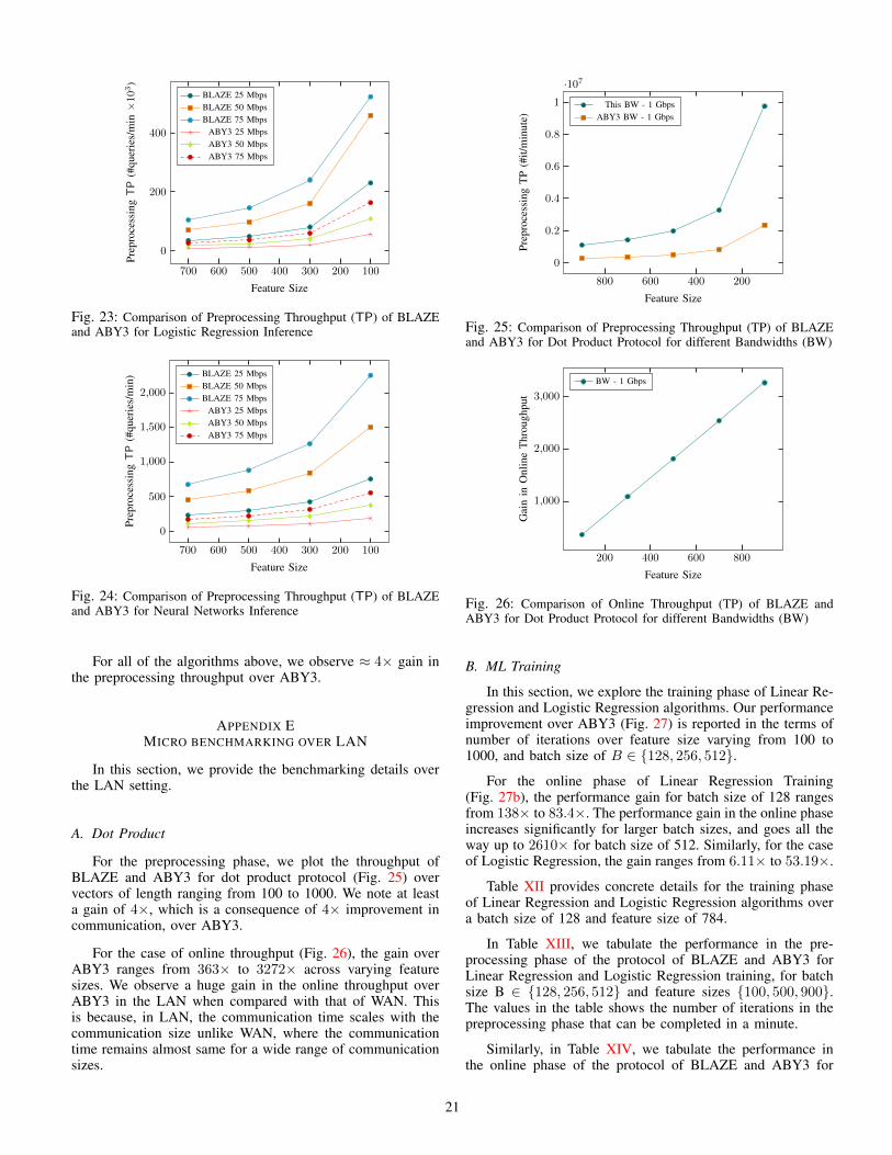
100200300400500600700

0

200

400

Feature Size

Prep

roce

ssin

gT

P(#

quer

ies/

min×

103)

BLAZE 25 MbpsBLAZE 50 MbpsBLAZE 75 Mbps

ABY3 25 MbpsABY3 50 MbpsABY3 75 Mbps

Fig. 23: Comparison of Preprocessing Throughput (TP) of BLAZEand ABY3 for Logistic Regression Inference

100200300400500600700

0

500

1,000

1,500

2,000

Feature Size

Prep

roce

ssin

gT

P(#

quer

ies/

min

) BLAZE 25 MbpsBLAZE 50 MbpsBLAZE 75 Mbps

ABY3 25 MbpsABY3 50 MbpsABY3 75 Mbps

Fig. 24: Comparison of Preprocessing Throughput (TP) of BLAZEand ABY3 for Neural Networks Inference

For all of the algorithms above, we observe ≈ 4× gain inthe preprocessing throughput over ABY3.

APPENDIX EMICRO BENCHMARKING OVER LAN

In this section, we provide the benchmarking details overthe LAN setting.

A. Dot Product

For the preprocessing phase, we plot the throughput ofBLAZE and ABY3 for dot product protocol (Fig. 25) overvectors of length ranging from 100 to 1000. We note at leasta gain of 4×, which is a consequence of 4× improvement incommunication, over ABY3.

For the case of online throughput (Fig. 26), the gain overABY3 ranges from 363× to 3272× across varying featuresizes. We observe a huge gain in the online throughput overABY3 in the LAN when compared with that of WAN. Thisis because, in LAN, the communication time scales with thecommunication size unlike WAN, where the communicationtime remains almost same for a wide range of communicationsizes.

200400600800

0

0.2

0.4

0.6

0.8

1

·107

Feature Size

Prep

roce

ssin

gT

P(#

it/m

inut

e)

This BW - 1 GbpsABY3 BW - 1 Gbps

Fig. 25: Comparison of Preprocessing Throughput (TP) of BLAZEand ABY3 for Dot Product Protocol for different Bandwidths (BW)

200 400 600 800

1,000

2,000

3,000

Feature Size

Gai

nin

Onl

ine

Thr

ough

put

BW - 1 Gbps

Fig. 26: Comparison of Online Throughput (TP) of BLAZE andABY3 for Dot Product Protocol for different Bandwidths (BW)

B. ML Training

In this section, we explore the training phase of Linear Re-gression and Logistic Regression algorithms. Our performanceimprovement over ABY3 (Fig. 27) is reported in the terms ofnumber of iterations over feature size varying from 100 to1000, and batch size of B ∈ {128, 256, 512}.

For the online phase of Linear Regression Training(Fig. 27b), the performance gain for batch size of 128 rangesfrom 138× to 83.4×. The performance gain in the online phaseincreases significantly for larger batch sizes, and goes all theway up to 2610× for batch size of 512. Similarly, for the caseof Logistic Regression, the gain ranges from 6.11× to 53.19×.

Table XII provides concrete details for the training phaseof Linear Regression and Logistic Regression algorithms overa batch size of 128 and feature size of 784.

In Table XIII, we tabulate the performance in the pre-processing phase of the protocol of BLAZE and ABY3 forLinear Regression and Logistic Regression training, for batchsize B ∈ {128, 256, 512} and feature sizes {100, 500, 900}.The values in the table shows the number of iterations in thepreprocessing phase that can be completed in a minute.

Similarly, in Table XIV, we tabulate the performance inthe online phase of the protocol of BLAZE and ABY3 for

21

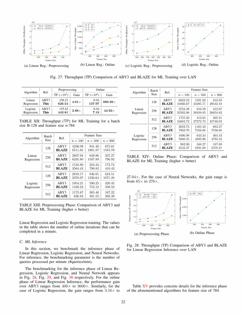
200400600800

0

1

2

3

4

5

·106

Feature Size

Offl

ine

Thr

ough

put

(#L

inR

eg/m

in) This B - 128/256/512

ABY3 B - 128/256/512

(a) Linear Reg.: Preprocessing

200 400 600 800

0

500

1,000

1,500

2,000

2,500

Feature Size

Gai

nin

Onl

ine

Thr

ough

put

B - 128B - 256B - 512

(b) Linear Reg.: Online

300400500600700800900

2

4

6

8

·105

Feature Size

Offl

ine

Thr

ough

put

(#L

ogR

eg/m

in) This B - 128/256/512

ABY3 B - 128/256/512

(c) Logistic Reg.: Preprocessing

200 400 600 800

10

20

30

40

50

Feature Size

Gai

nin

Onl

ine

Thr

ough

put

B - 128 / 256 / 512

(d) Logistic Reg.: Online

Fig. 27: Throughput (TP) Comparison of ABY3 and BLAZE for ML Training over LAN

Algorithm Ref.Preprocessing Online

TP (×103) Gain TP (×106) Gain

LinearRegression

ABY3 156.214.01× 0.16

880.28×This 626.54 137.97

LogisticRegression

ABY3 155.422.86× 0.16

44.92×This 443.81 7.19

TABLE XII: Throughput (TP) for ML Training for a batchsize B-128 and feature size n-784

Algorithm BatchSize Ref.

Feature Size

n = 100 n = 500 n = 900

LinearRegression

128 ABY3 4236.09 941.40 675.01BLAZE 8511.85 1961.87 1585.79

256 ABY3 2807.94 649.96 337.27BLAZE 6335.80 1587.89 790.92

512 ABY3 1516.80 324.34 172.74BLAZE 3564.43 790.82 410.43

LogisticRegression

128 ABY3 2810.17 846.01 624.51BLAZE 2378.97 1230.64 1071.28

256 ABY3 1954.21 590.25 320.45BLAZE 1169.23 753.12 509.58

512 ABY3 1175.87 305.40 167.22BLAZE 636.94 391.55 268.39

TABLE XIII: Preprocessing Phase: Comparison of ABY3 andBLAZE for ML Training (higher = better)

Linear Regression and Logistic Regression training. The valuesin the table shows the number of online iterations that can becompleted in a minute.

C. ML Inference

In this section, we benchmark the inference phase ofLinear Regression, Logistic Regression, and Neural Networks.For inference, the benchmarking parameter is the number ofqueries processed per minute (#queries/min).

The benchmarking for the inference phase of Linear Re-gression, Logistic Regression, and Neural Network appearsin Fig. 28, Fig. 29, and Fig. 30 respectively. For the onlinephase of Linear Regression Inference, the performance gainover ABY3 ranges from 400× to 3600×. Similarly, for thecase of Logistic Regression, the gain ranges from 3.16× to

Algorithm BatchSize Ref.

Feature Size

n = 100 n = 500 n = 900

LinearRegression

128 ABY3 6622.52 1591.93 810.58BLAZE 41666.67 34285.71 29542.10

256 ABY3 3724.39 810.59 412.67BLAZE 35502.96 30456.85 26654.82

512 ABY3 1755.93 412.65 205.21BLAZE 34883.72 27272.73 25740.03

LogisticRegression

128 ABY3 2623.75 1165.43 683.27BLAZE 7863.70 7556.68 7556.68

256 ABY3 1696.98 643.34 364.43BLAZE 5008.35 4893.96 4783.16

512 ABY3 982.90 348.27 187.89BLAZE 2542.37 2491.69 2478.21

TABLE XIV: Online Phase: Comparison of ABY3 andBLAZE for ML Training (higher = better)

27.04×. For the case of Neural Networks, the gain range isfrom 65× to 276×.

200400600800

0

0.2

0.4

0.6

0.8

1

·104

Feature Size

Prep

roce

ssin

gT

P(#

quer

ies/

min

) This BW - 1 GbpsABY3 BW - 1 Gbps

(a) Preprocessing Phase

200 400 600 800

1,000

2,000

3,000

Feature Size

Gai

nin

Onl

ine

Thr

ough

put

BW - 1 Gbps

(b) Online Phase

Fig. 28: Throughput (TP) Comparison of ABY3 and BLAZEfor Linear Regression Inference over LAN

Table XV provides concrete details for the inference phaseof the aforementioned algorithms for feature size of 784.

22

300400500600700800900200

400

600

800

1,000

Feature Size

Prep

roce

ssin

gT

P(#

quer

ies/

min×

103)

This BW - 1 GbpsABY3 BW - 1 Gbps

(a) Preprocessing Phase

300 400 500 600 700 800 900

10

15

20

25

Feature Size

Gai

nin

Onl

ine

Thr

ough

put

BW - 1 Gbps

(b) Online Phase

Fig. 29: Throughput (TP) Comparison of ABY3 and BLAZEfor Logistic Regression Inference over LAN

2004006008000

10

20

30

Feature Size

Prep

roce

ssin

gT

P(#

quer

ies/

min×

103)

BLAZE - 1 GbpsABY3 - 1 Gbps

(a) Preprocessing Phase

200 400 600 80050

100

150

200

250

Feature Size

Gai

nin

Onl

ine

Thr

ough

put

1 Gbps

(b) Online Phase

Fig. 30: Throughput (TP) Comparison of ABY3 and BLAZEfor Neural Network Inference over LAN

Algorithm Ref.Preprocessing Online

TP (×103) Gain TP (×106) Gain

LinearRegression

ABY3 311.3844.02× 0.31

3136×This 1252.28 983.04

LogisticRegression

ABY3 308.252.23× 0.31

23.57×This 686.93 7.33

NeuralNetworks

ABY3 2.044.01× 0.003

245.74×This 8.14 0.65

TABLE XV: Throughput (TP) for ML Inference for a featuresize of n-784

APPENDIX FSECURITY OF OUR CONSTRUCTIONS

In this section, we prove the security of our constructionsusing the standard real/ideal world paradigm. Our proofs workin the {Fsetup,FmulZK}-hybrid model, where Fsetup (Fig. 17)and FmulZK (Fig. 20) denote the ideal-world functionalities forthe shared key-setup and ΠmulZK protocol respectively.

Let A denote the real-world adversary corrupting one ofthe servers in P . We use S to denote an ideal-world adversary(simulator) for A, who plays the roles of the honest serversand simulates the messages received by A during the protocol.The simulator initializes a boolean variable flag = 0, whichindicates whether an honest server aborts during the protocol.For the case of abort, flag is set to 1. To distinguish thesimulators for various constructions, we use the correspondingprotocol name as the subscript of S.

For a circuit ckt, the simulation proceeds as follows: The

simulation start with the input sharing phase, where S sets theinput of honest parties to 0. From the sharing protocol Πsh, Sextracts the input of A (details are provided in the simulationfor Πsh protocol). This enables S to obtain the entire input forthe ckt, which in turn enables S to know all of the intermediatevalues and the output of the circuit. Looking ahead, S will beusing these information to simulate each of the components ofthe ckt.

We now provide the simulation details for each of theconstructions in detail. For each of these, we provide thesimulation for a corrupt P0 and a corrupt P1 separately. Thecase for P2 is similar to that of P1 and we omit details of thesame.

A. Sharing Protocol

The ideal functionality realising protocol Πsh is presentedin Fig. 31.

Fsh interacts with the servers in P and the adversary S. Fsh

receives the input v from server Pi while it receives ⊥ from theother servers. If v = ⊥, then send ⊥ to every server, else proceedwith the computation.

Computation of output: Randomly select [αv]1 , [αv]2 , γv fromZ2` and set βv = v + [αv]1 + [αv]2. The output shares are set as:

JvK0 = ([αv]1 , [αv]2 , βv + γv),

JvK1 = ([αv]1 , βv, γv),

JvK2 = ([αv]2 , βv, γv)

Output to adversary: If S sends abort, then send (Output,⊥)to all the servers. Otherwise, send (Output, JvKS) to the adversaryS, where JvKS denotes the share of v corresponding to the corruptserver.

Output to selected honest servers: Receive (select, {I}) fromadversary S, where {I} denotes a subset of the honest servers.If an honest server Pi belongs to I , send (Output,⊥), else send(Output, JvKi), where JvKi denotes the share of v correspondingto the honest server Pi.

Functionality Fsh

Fig. 31: Functionality for protocol Πsh

The simulator for the case of corrupt P0 appears inFig. 32.

Preprocessing Phase: Ssh emulates Fsetup and gives the keys(k01, k02 and kP) to A. By emulating Fsetup, it learns the α-valuescorresponding to input v. If Pi = P0, then Ssh computes γv usingthe key kP , else it samples a random γv on behalf of P1, P2.

Online Phase:

– If Pi = P0, Ssh receives βv of behalf of P1, P2. Ssh sets flag =1 if the received values mismatch. Else, it computes the inputv = βv − αv.

– If Pi 6= P0, Ssh sets v = 0 by assigning βv = αv. Ssh sendsβv+γv and H(βv+γv) to A on behalf of P1 and P2 respectively.

Simulator Ssh

23

If flag = 0 and Pi = P0, Ssh invokes Fsh with input v on behalfof P0. Else it invokes Fsh with input ⊥ on behalf of P0.

Fig. 32: Simulator Ssh for the case of corrupt P0

The simulator for the case of corrupt P1 appears inFig. 33.

Preprocessing Phase: Ssh emulates Fsetup and gives the keys(k01, k12 and kP) to A. By emulating Fsetup, it learns the α-valuescorresponding to input v. If Pi = P0, then Ssh computes γv usingthe key kP , else it computes γv using the key k12 .

Online Phase:

– If Pi = P1, then Ssh receives βv on behalf of P2 and βv + γvon behalf of P0. Ssh sets flag = 1 if the received values areinconsistent. Else, it computes the input v = βv − αv.

– If Pi = Pj for j ∈ {0, 2}, then– Ssh sets v = 0 by assigning βv = αv and sends βv to A on

behalf of Pj .

– Ssh sends H(βv) to A and receives H(βv)′ from A on behalf

of P2.

– Ssh receives β′v + γ′v from S on behalf of P0.

– Ssh sets flag = 1 if either H(βv)′ 6= H(βv) or βv + γv 6=

β′v + γ′v.

If flag = 0 and Pi = P1, Ssh invokes Fsh with input v on behalfof P1. Else it invokes Fsh with input ⊥ on behalf of P1.

Simulator Ssh

Fig. 33: Simulator Ssh for the case of corrupt P1

B. Joint Sharing Protocol

The ideal functionality realising protocol Πjsh is presentedin Fig. 34.

Fjsh interacts with the servers in P and the adversary S. Fjsh

receives the input v from servers Pi, Pj while it receives ⊥ fromthe third server. If the values received from Pi, Pj mismatch, thensend ⊥ to every server, else proceed with the computation.

Computation of output: Randomly select [αv]1 , [αv]2 , γv fromZ2` and set βv = v + [αv]1 + [αv]2. The output shares are set as:

JvK0 = ([αv]1 , [αv]2 , βv + γv),

JvK1 = ([αv]1 , βv, γv),

JvK2 = ([αv]2 , βv, γv)

Output to adversary: If S sends abort, then send (Output,⊥)to all the servers. Otherwise, send (Output, JvKS) to the adversaryS, where JvKS denotes the share of v corresponding to the corruptserver.

Output to selected honest servers: Receive (select, {I}) fromadversary S, where {I} denotes a subset of the honest servers.If an honest server Pi belongs to I , send (Output,⊥), else send(Output, JvKi), where JvKi denotes the share of v correspondingto the honest server Pi.

Functionality Fjsh

Fig. 34: Functionality for protocol Πjsh

The simulator for the case of corrupt P0 appears inFig. 35.

Preprocessing Phase: Sjsh emulates Fsetup and gives the keys(k01, k02 and kP) to A. By emulating Fsetup, it learns the α-valuescorresponding to input v. Sjsh samples a random γv on behalf ofP1, P2.

Online Phase:

– If (Pi, Pj) = (P1, P0), then– Sjsh computes βv = v + [αv]1 + [αv]2 on behalf of P1.

– Sjsh receives H(β′v) from A on behalf of P2 and sets flag = 1if H(βv)

′ 6= H(βv).

– Sjsh then sends βv + γv and H(βv + γv) to A on behalf ofP1 and P2 respectively.

– The case for (Pi, Pj) = (P2, P0) follows similarly.

– If (Pi, Pj) = (P1, P2), then Sjsh sets v = 0 by assigning βv =[αv]1 + [αv]2. Sjsh then sends βv + γv and H(βv + γv) to A onbehalf of P1 and P2 respectively.

If flag = 0 and Pj = P0, Sjsh invokes Fjsh with input v on behalfof P0. Else it invokes Fjsh with input ⊥ on behalf of P0.

Simulator Sjsh

Fig. 35: Simulator Sjsh for the case of corrupt P0

The simulator for the case of corrupt P1 appears inFig. 36.

Preprocessing Phase: Sjsh emulates Fsetup and gives the keys(k01, k12 and kP) to A. By emulating Fsetup, it learns the α-valuescorresponding to input v. Sjsh computes γv using the key k12.

Online Phase:

– If (Pi, Pj) = (P1, P0), then– Sjsh computes βv = v + [αv]1 + [αv]2 on behalf of P0.

– Sjsh receives β′v from A on behalf of P2 and sets flag = 1 ifβ′v 6= βv.

– Sjsh receives β′v+γ′v fromA on behalf of P0 and sets flag = 1if β′v + γ′v 6= βv + γv.

– If (Pi, Pj) = (P1, P2), then Sjsh receives β′v + γ′v from A onbehalf of P0 and sets flag = 1 if β′v + γ′v 6= βv + γv.

– If (Pi, Pj) = (P2, P0), then Sjsh sets v = 0 by assigning βv =[αv]1 + [αv]2. Sjsh then sends βv and H(βv) to A on behalf ofP2 and P0 respectively.

If flag = 0 and Pi = P1, Ssh invokes Fjsh with input v on behalfof P1. Else it invokes Fjsh with input ⊥ on behalf of P1.

Simulator Sjsh

Fig. 36: Simulator Sjsh for the case of corrupt P1

24

C. Reconstruction Protocol

The ideal functionality realising protocol Πrec is presentedin Fig. 37.

Frec interacts with the servers in P and the adversary S. Frec

receives the 〈·〉-shares of value v from server Pi for i ∈ {0, 1, 2}.The shares are

〈v〉0 = ([αv]1 , [αv]2),

〈v〉1 = ([αv]′1 , β

′v),

〈v〉2 = ([αv]′2 , β

′′v )

Frec sends ⊥ to every server if either of the following conditionis met: i) [αv]1 6= [αv]

′1, ii) [αv]2 6= [αv]

′2, or iii) β′v 6= β′′v . Else it

proceeds with the computation.

Computation of output: Set v = βv − [αv]1 − [αv]2.

Output to adversary: If S sends abort, then send (Output,⊥)to all the servers. Otherwise, send (Output, v) to the adversary S.

Output to selected honest servers: Receive (select, {I}) fromadversary S, where {I} denotes a subset of the honest servers.If an honest server Pi belongs to I , send (Output,⊥), else send(Output, v).

Functionality Frec

Fig. 37: Functionality for protocol Πrec

The simulator for the case of corrupt P0 appears in Fig. 38.As mentioned in the beginning of this section, S knows all ofthe intermediate values and the output of the ckt. S uses thisinformation to simulate the Πrec protocol.

Online Phase:

– Srec sends βv and H(βv) to A on behalf of P1 and P2

respectively.

– Srec receives H([α′v]2) and [αv]′1 from A on behalf of P1 and

P2 respectively. Srec sets flag = 1 if either H([α′v]1) 6= H([αv]1)or [αv]

′2 6= [αv]2.

If flag = 0, Srec invokes Frec with input ([αv]1 , [αv]2) on behalfof P0. Else it invokes Frec with input ⊥ on behalf of P0.

Simulator Srec

Fig. 38: Simulator Srec for the case of corrupt P0

The simulator for the case of corrupt P1 appears inFig. 39.

Online Phase:

– Srec sends [αv]2 and H([αv]2) to A on behalf of P2 and P0

respectively.

– Srec receives H([α′v]1) and β′v from A on behalf of P2 and P0

respectively. Srec sets flag = 1 if either H([α′v]1) 6= H([αv]1) orβ′v 6= βv.

Simulator Srec

If flag = 0, Srec invokes Frec with input ([αv]1 , βv) on behalf ofP1. Else it invokes Frec with input ⊥ on behalf of P1.

Fig. 39: Simulator Srec for the case of corrupt P1

D. Multiplication

The ideal functionality realising protocol Πmult is presentedin Fig. 40.

Fmult interacts with the servers in P and the adversary S. Fmult

receives J·K-shares of values x and y from the servers as input. IfFmult receives ⊥ from S, then send ⊥ to every server, else proceedwith the computation.

Computation of output: Compute x = βx − [αx]1 − [αx]2 , y =βy− [αy]1− [αy]2 and set z = xy. Randomly select [αz]1 , [αz]2 , γzfrom Z2` and set βz = z + [αz]1 + [αz]2. The output shares are setas:

JzK0 = ([αz]1 , [αz]2 , βz + γz),

JzK1 = ([αz]1 , βz, γz),

JzK2 = ([αz]2 , βz, γz)

Output to adversary: If S sends abort, then send (Output,⊥)to all the servers. Otherwise, send (Output, JzKS) to the adversaryS, where JzKS denotes the share of z corresponding to the corruptserver.

Output to selected honest servers: Receive (select, {I}) fromadversary S, where {I} denotes a subset of the honest servers.If an honest server Pi belongs to I , send (Output,⊥), else send(Output, JzKi), where JzKi denotes the share of z corresponding tothe honest server Pi.

Functionality Fmult

Fig. 40: Functionality for protocol Πmult

The simulator for the case of corrupt P0 appears inFig. 41.

Preprocessing Phase:

– Smult computes [αz]1 and [αz]2 using the keys k01 and k02respectively. Also, Smult samples a random γz on behalf of P1, P2

and prepares the 〈·〉-shares of d, e honestly.

– Smult emulates FmulZK and gives ([λf ]1 , [λf ]2) to A. Smult thencomputes the values ψ, χ followed by computing Γxy = γxαy +γyαx + ψ − χ.

Online Phase:

– Smult receives H(β?z ) from A on behalf of P1 and P2. Smult

sets flag = 1 if either the received hash values are inconsistentor if H(β?

z ) 6= H(βz − βxβy + ψ).

– Else, Smult sends βz + γz and H(βz + γz) to A on behalf of P1

and P2 respectively.

If flag = 0, Smult invokes Fmult with input (JxK0, JyK0) on behalfof P0. Else it invokes Fmult with input ⊥ on behalf of P0.

Simulator Smult

Fig. 41: Simulator for the case of corrupt P0

25

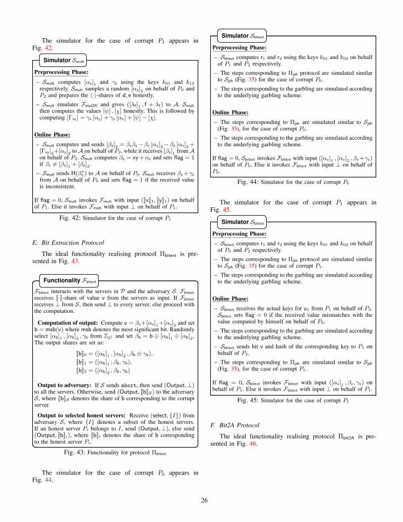
The simulator for the case of corrupt P1 appears inFig. 42.

Preprocessing Phase:

– Smult computes [αz]1 and γz using the keys k01 and k12respectively. Smult samples a random [αz]2 on behalf of P0 andP2 and prepares the 〈·〉-shares of d, e honestly.

– Smult emulates FmulZK and gives ([λf ]1 , f + λf) to A. Smult

then computes the values [ψ] , [χ] honestly. This is followed bycomputing [Γxy] = γx [αy] + γy [αx] + [ψ]− [χ].

Online Phase:

– Smult computes and sends [βz]2 = βxβy−βx [αy]2−βy [αx]2 +[Γxy]2+[αz]2 toA on behalf of P2, while it receives [βz]1 fromAon behalf of P2. Smult computes βz = xy +αz and sets flag = 1if βz 6= [βz]1 + [βz]2.

– Smult sends H(β?z ) to A on behalf of P0. Smult receives βz +γz

from A on behalf of P0 and sets flag = 1 if the received valueis inconsistent.

If flag = 0, Smult invokes Fmult with input (JxK1, JyK1) on behalfof P1. Else it invokes Fmult with input ⊥ on behalf of P1.

Simulator Smult

Fig. 42: Simulator for the case of corrupt P1

E. Bit Extraction Protocol

The ideal functionality realising protocol Πbitext is pre-sented in Fig. 43.

Fbitext interacts with the servers in P and the adversary S. Fbitext

receives J·K-share of value v from the servers as input. If Fbitext

receives ⊥ from S, then send ⊥ to every server, else proceed withthe computation.

Computation of output: Compute v = βv+[αv]1+[αv]2 and setb = msb(v) where msb denotes the most significant bit. Randomlyselect [αb]1 , [αb]2 , γb from Z21 and set βb = b ⊕ [αb]1 ⊕ [αb]2.The output shares are set as:

JbK0 = ([αb]1 , [αb]2 , βb ⊕ γb),JbK1 = ([αb]1 , βb, γb),

JbK2 = ([αb]2 , βb, γb)

Output to adversary: If S sends abort, then send (Output,⊥)to all the servers. Otherwise, send (Output, JbKS) to the adversaryS, where JbKS denotes the share of b corresponding to the corruptserver.

Output to selected honest servers: Receive (select, {I}) fromadversary S, where {I} denotes a subset of the honest servers.If an honest server Pi belongs to I , send (Output,⊥), else send(Output, JbKi), where JbKi denotes the share of b correspondingto the honest server Pi.

Functionality Fbitext

Fig. 43: Functionality for protocol Πbitext

The simulator for the case of corrupt P0 appears inFig. 44.

Preprocessing Phase:

– Sbitext computes r1 and r2 using the keys k01 and k02 on behalfof P1 and P2 respectively.

– The steps corresponding to Πjsh protocol are simulated similarto Sjsh (Fig. 35) for the case of corrupt P0.

– The steps corresponding to the garbling are simulated accordingto the underlying garbling scheme.

Online Phase:

– The steps corresponding to Πjsh are simulated similar to Sjsh(Fig. 35), for the case of corrupt P0.

– The steps corresponding to the garbling are simulated accordingto the underlying garbling scheme.

If flag = 0, Sbitext invokes Fbitext with input ([αv]1 , [αv]2 , βv+γv)on behalf of P0. Else it invokes Fbitext with input ⊥ on behalf ofP0.

Simulator Sbitext

Fig. 44: Simulator for the case of corrupt P0

The simulator for the case of corrupt P1 appears inFig. 45.

Preprocessing Phase:

– Sbitext computes r1 and r2 using the keys k01 and k02 on behalfof P0 and P2 respectively.

– The steps corresponding to Πjsh protocol are simulated similarto Sjsh (Fig. 35) for the case of corrupt P1.

– The steps corresponding to the garbling are simulated accordingto the underlying garbling scheme.

Online Phase:

– Sbitext receives the actual keys for u1 from P1 on behalf of P2.Sbitext sets flag = 0 if the received value mismatches with thevalue computed by himself on behalf of P0.

– The steps corresponding to the garbling are simulated accordingto the underlying garbling scheme.

– Sbitext sends bit v and hash of the corresponding key to P1 onbehalf of P2.

– The steps corresponding to Πjsh are simulated similar to Sjsh(Fig. 35), for the case of corrupt P1.

If flag = 0, Sbitext invokes Fbitext with input ([αv]1 , βv, γv) onbehalf of P1. Else it invokes Fbitext with input ⊥ on behalf of P1.

Simulator Sbitext

Fig. 45: Simulator for the case of corrupt P1

F. Bit2A Protocol

The ideal functionality realising protocol Πbit2A is pre-sented in Fig. 46.

26

Fbit2A interacts with the servers in P and the adversary S. Fbit2A

receives J·KB-share of a bit b from the servers as input. If Fbit2A

receives ⊥ from S, then send ⊥ to every server, else proceed withthe computation.

Computation of output: Compute b = βb ⊕ [αb]1 ⊕ [αb]2.Let (b)A denotes the value of bit b over an arithmetic ringZ2` . Randomly select

[α(b)A

]1,[α(b)A

]2, γ(b)A from Z2` and set

β(b)A = (b)A +[α(b)A

]1

+[α(b)A

]2. The output shares are set

as:

J(b)AK0 = ([α(b)A

]1,[α(b)A

]2, β(b)A + γ(b)A),

J(b)AK1 = ([α(b)A

]1, β(b)A , γ(b)A),

J(b)AK2 = ([α(b)A

]2, β(b)A , γ(b)A)

Output to adversary: If S sends abort, then send (Output,⊥)to all the servers. Otherwise, send (Output, J(b)AKS) to the adver-sary S, where J(b)AKS denotes the share of (b)A correspondingto the corrupt server.

Output to selected honest servers: Receive (select, {I}) fromadversary S, where {I} denotes a subset of the honest servers.If an honest server Pi belongs to I , send (Output,⊥), elsesend (Output, J(b)AKi), where J(b)AKi denotes the share of (b)A

corresponding to the honest server Pi.

Functionality Fbit2A

Fig. 46: Functionality for protocol Πbit2A

The simulator for the case of corrupt P0 appears inFig. 47.

Preprocessing Phase:

– The steps corresponding to Πjsh and Πmult protocols are sim-ulated similar to Sjsh (Fig. 35) and Smult (Fig. 41) respectively,for the case of corrupt P0.

Online Phase:

– The steps corresponding to Πjsh and Πmult protocols are sim-ulated similar to Sjsh (Fig. 35) and Smult (Fig. 41) respectively,for the case of corrupt P0.

If flag = 0, Sbit2A invokes Fbit2A with input JbKB0 on behalf of P0.Else it invokes Fbit2A with input ⊥ on behalf of P0.

Simulator Sbit2A

Fig. 47: Simulator for the case of corrupt P0

The simulator for the case of corrupt P1 appears inFig. 48.

Preprocessing Phase:

– The steps corresponding to Πjsh and Πmult protocols are sim-ulated similar to Sjsh (Fig. 36) and Smult (Fig. 42) respectively,for the case of corrupt P1.

Online Phase:

– The steps corresponding to Πjsh and Πmult protocols are sim-ulated similar to Sjsh (Fig. 36) and Smult (Fig. 42) respectively,for the case of corrupt P1.

Simulator Sbit2A

If flag = 0, Sbit2A invokes Fbit2A with input JbKB1 on behalf of P1.Else it invokes Fbit2A with input ⊥ on behalf of P1.

Fig. 48: Simulator for the case of corrupt P1

G. Dot Product Protocol

The ideal functionality realising protocol Πdotp is presentedin Fig. 49.

Fdotp interacts with the servers in P and the adversary S. Fdotp

receives J·K-shares of vectors ~x and ~y from the servers as input.Here ~x and ~y are n-length vectors. If Fdotp receives ⊥ from S,then send ⊥ to every server, else proceed with the computation.

Computation of output: Compute xi = βxi − [αxi ]1 −[αxi ]2 , yi = βyi − [αyi ]1 − [αyi ]2 for i ∈ [n] and set z =∑n

i=1 xiyi. Randomly select [αz]1 , [αz]2 , γz from Z2` and setβz = z + [αz]1 + [αz]2. The output shares are set as:

JzK0 = ([αz]1 , [αz]2 , βz + γz),

JzK1 = ([αz]1 , βz, γz),

JzK2 = ([αz]2 , βz, γz)

Output to adversary: If S sends abort, then send (Output,⊥)to all the servers. Otherwise, send (Output, JzKS) to the adversaryS, where JzKS denotes the share of z corresponding to the corruptserver.

Output to selected honest servers: Receive (select, {I}) fromadversary S, where {I} denotes a subset of the honest servers.If an honest server Pi belongs to I , send (Output,⊥), else send(Output, JzKi), where JzKi denotes the share of z corresponding tothe honest server Pi.

Functionality Fdotp

Fig. 49: Functionality for protocol Πsh

The simulator for the case of corrupt P0 appears inFig. 50.

Preprocessing Phase:

– For the preprocessing corresponding to each of the n mul-tiplications, Sdotp simulates similar to the simulation for thepreprocessing phase of Πmult protocol given in Smult (Fig. 41),for the case of corrupt P0.

Online Phase:

– Sdotp receives H(β?z ) from A on behalf of P1 and P2. Sdotp

sets flag = 1 if either the received hash values are inconsistentor if H(β?

z ) 6= H(βz −∑n

i=1 βxiβyi + ψ).

– Else, Sdotp sends βz + γz and H(βz + γz) to A on behalf of P1

and P2 respectively.

If flag = 0, Sdotp invokes Fdotp with input (J~xK0, J~yK0) on behalfof P0. Else it invokes Fdotp with input ⊥ on behalf of P0.

Simulator Sdotp

Fig. 50: Simulator for the case of corrupt P0

The simulator for the case of corrupt P1 appears inFig. 51.

27

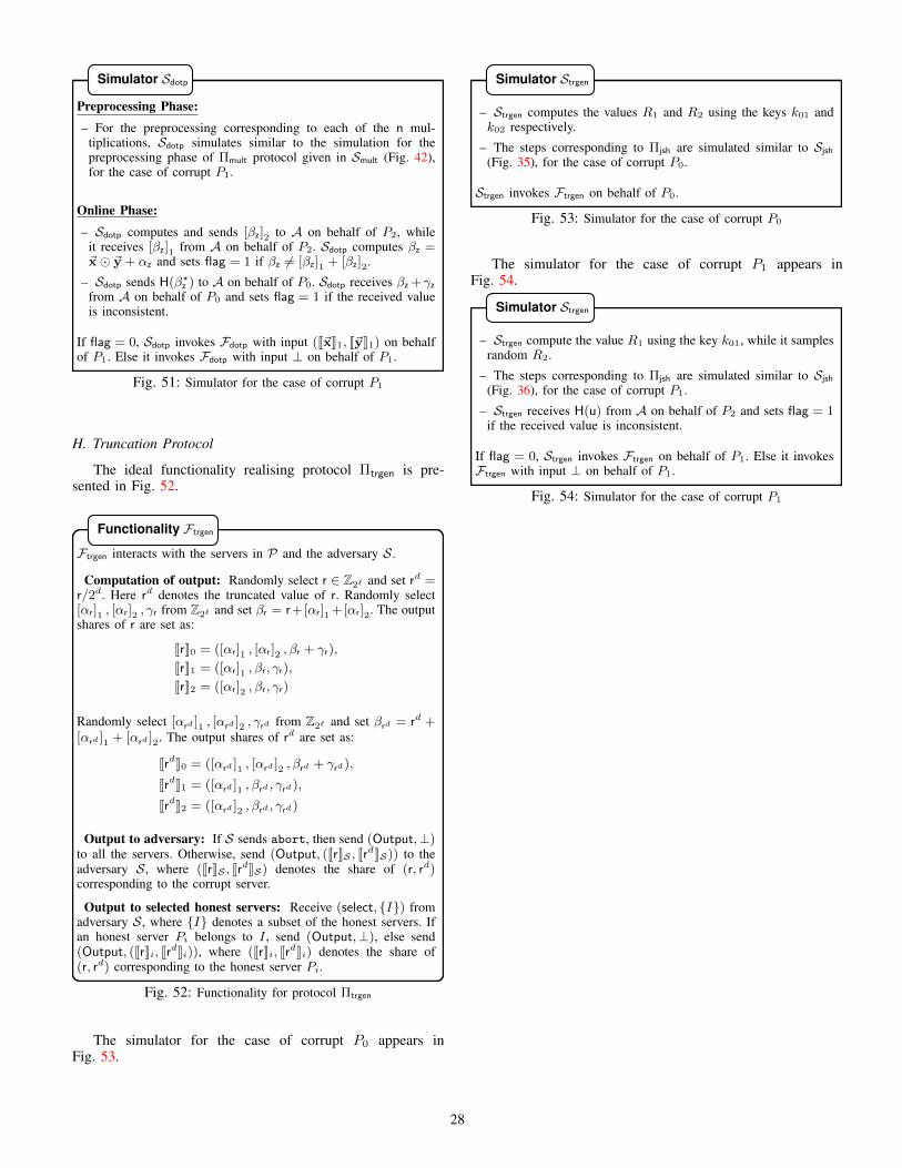
Preprocessing Phase:

– For the preprocessing corresponding to each of the n mul-tiplications, Sdotp simulates similar to the simulation for thepreprocessing phase of Πmult protocol given in Smult (Fig. 42),for the case of corrupt P1.

Online Phase:

– Sdotp computes and sends [βz]2 to A on behalf of P2, whileit receives [βz]1 from A on behalf of P2. Sdotp computes βz =~x� ~y + αz and sets flag = 1 if βz 6= [βz]1 + [βz]2.

– Sdotp sends H(β?z ) to A on behalf of P0. Sdotp receives βz +γz

from A on behalf of P0 and sets flag = 1 if the received valueis inconsistent.

If flag = 0, Sdotp invokes Fdotp with input (J~xK1, J~yK1) on behalfof P1. Else it invokes Fdotp with input ⊥ on behalf of P1.

Simulator Sdotp

Fig. 51: Simulator for the case of corrupt P1

H. Truncation Protocol

The ideal functionality realising protocol Πtrgen is pre-sented in Fig. 52.

Ftrgen interacts with the servers in P and the adversary S.

Computation of output: Randomly select r ∈ Z2` and set rd =r/2d. Here rd denotes the truncated value of r. Randomly select[αr]1 , [αr]2 , γr from Z2` and set βr = r+[αr]1 +[αr]2. The outputshares of r are set as:

JrK0 = ([αr]1 , [αr]2 , βr + γr),

JrK1 = ([αr]1 , βr, γr),

JrK2 = ([αr]2 , βr, γr)

Randomly select [αrd ]1 , [αrd ]2 , γrd from Z2` and set βrd = rd +[αrd ]1 + [αrd ]2. The output shares of rd are set as:

JrdK0 = ([αrd ]1 , [αrd ]2 , βrd + γrd),

JrdK1 = ([αrd ]1 , βrd , γrd),

JrdK2 = ([αrd ]2 , βrd , γrd)

Output to adversary: If S sends abort, then send (Output,⊥)to all the servers. Otherwise, send (Output, (JrKS , JrdKS)) to theadversary S, where (JrKS , JrdKS) denotes the share of (r, rd)corresponding to the corrupt server.

Output to selected honest servers: Receive (select, {I}) fromadversary S, where {I} denotes a subset of the honest servers. Ifan honest server Pi belongs to I , send (Output,⊥), else send(Output, (JrKi, JrdKi)), where (JrKi, JrdKi) denotes the share of(r, rd) corresponding to the honest server Pi.

Functionality Ftrgen

Fig. 52: Functionality for protocol Πtrgen

The simulator for the case of corrupt P0 appears inFig. 53.

– Strgen computes the values R1 and R2 using the keys k01 andk02 respectively.

– The steps corresponding to Πjsh are simulated similar to Sjsh(Fig. 35), for the case of corrupt P0.

Strgen invokes Ftrgen on behalf of P0.

Simulator Strgen

Fig. 53: Simulator for the case of corrupt P0

The simulator for the case of corrupt P1 appears inFig. 54.

– Strgen compute the value R1 using the key k01, while it samplesrandom R2.

– The steps corresponding to Πjsh are simulated similar to Sjsh(Fig. 36), for the case of corrupt P1.

– Strgen receives H(u) from A on behalf of P2 and sets flag = 1if the received value is inconsistent.

If flag = 0, Strgen invokes Ftrgen on behalf of P1. Else it invokesFtrgen with input ⊥ on behalf of P1.

Simulator Strgen

Fig. 54: Simulator for the case of corrupt P1

28