black-box, functional testing · functional testing • rigorous specifications have another...
TRANSCRIPT
© Lionel Briand 2010 1
Black-Box, Functional Testing
© Lionel Briand 2010 2
Introduction • Based on the definition of what a program’s
specification, as opposed to its structure • Does the implementation correctly implement the
functionality as per the given system specifications?
• The notion of coverage can also be applied to functional testing
• Rigorous specifications have another benefit, they help functional testing, e.g., categorize inputs, derive expected outputs
• In other words, they help test case generation and test oracles
© Lionel Briand 2010 3
Outline
• Equivalence Class Partitioning • Boundary-Value Analysis • Category-Partition • Decision tables • Cause-Effect Graphs • Logic Functions
© Lionel Briand 2010 4
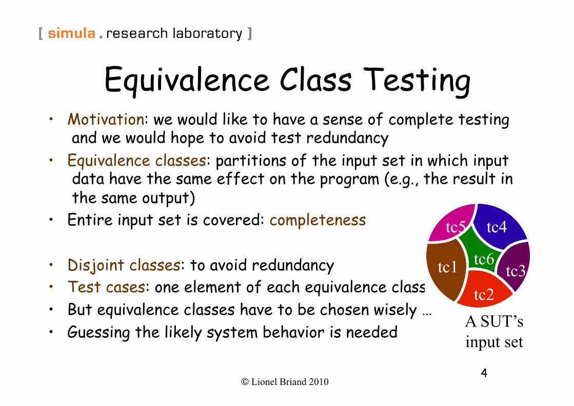
Equivalence Class Testing • Motivation: we would like to have a sense of complete testing
and we would hope to avoid test redundancy • Equivalence classes: partitions of the input set in which input
data have the same effect on the program (e.g., the result in the same output)
• Entire input set is covered: completeness
• Disjoint classes: to avoid redundancy • Test cases: one element of each equivalence class • But equivalence classes have to be chosen wisely … • Guessing the likely system behavior is needed A SUT’s
input set
tc1 tc2
tc3 tc6
tc4 tc5
© Lionel Briand 2010 5
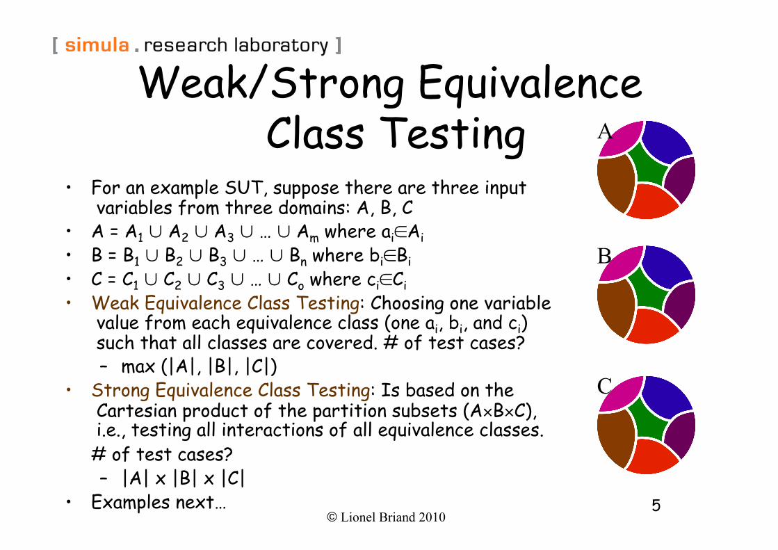
Weak/Strong Equivalence Class Testing
• For an example SUT, suppose there are three input variables from three domains: A, B, C
• A = A1 ∪ A2 ∪ A3 ∪ … ∪ Am where ai∈Ai • B = B1 ∪ B2 ∪ B3 ∪ … ∪ Bn where bi∈Bi • C = C1 ∪ C2 ∪ C3 ∪ … ∪ Co where ci∈Ci • Weak Equivalence Class Testing: Choosing one variable
value from each equivalence class (one ai, bi, and ci) such that all classes are covered. # of test cases? – max (|A|, |B|, |C|)
• Strong Equivalence Class Testing: Is based on the Cartesian product of the partition subsets (A×B×C), i.e., testing all interactions of all equivalence classes. # of test cases?
– |A| x |B| x |C| • Examples next…
A
B
C
© Lionel Briand 2010 6
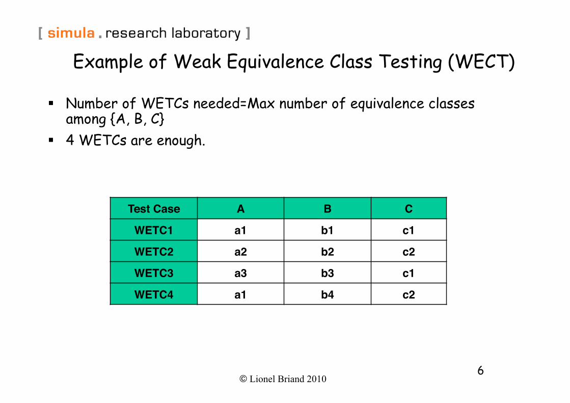
Example of Weak Equivalence Class Testing (WECT)
Test Case! A! B! C!
WETC1! a1! b1! c1!
WETC2! a2! b2! c2!
WETC3! a3! b3! c1!
WETC4! a1! b4! c2!
Number of WETCs needed=Max number of equivalence classes among {A, B, C}
4 WETCs are enough.
© Lionel Briand 2010 7
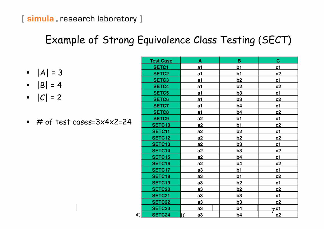
Example of Strong Equivalence Class Testing (SECT)
Test Case! A! B! C!SETC1! a1! b1! c1!SETC2! a1! b1! c2!SETC3! a1! b2! c1!SETC4! a1! b2! c2!SETC5! a1! b3! c1!SETC6! a1! b3! c2!SETC7! a1! b4! c1!SETC8! a1! b4! c2!SETC9! a2! b1! c1!
SETC10! a2! b1! c2!SETC11! a2! b2! c1!SETC12! a2! b2! c2!SETC13! a2! b3! c1!SETC14! a2! b3! c2!SETC15! a2! b4! c1!SETC16! a2! b4! c2!SETC17! a3! b1! c1!SETC18! a3! b1! c2!SETC19! a3! b2! c1!SETC20! a3! b2! c2!SETC21! a3! b3! c1!SETC22! a3! b3! c2!SETC23! a3! b4! c1!SETC24! a3! b4! c2!
|A| = 3
|B| = 4
|C| = 2
# of test cases=3x4x2=24
© Lionel Briand 2010 8
NextDate Example • NextDate is a function with three variables: month, day, year. It returns the date of the day after the input date. Limitation: 1812-2012
• Treatment Summary: if it is not the last day of the month, the next date function will simply increment the day value. At the end of a month, the next day is 1 and the month is incremented. At the end of the year, both the day and the month are reset to 1, and the year incremented. Finally, the problem of leap year makes determining the last day of a month interesting.
© Lionel Briand 2010 9
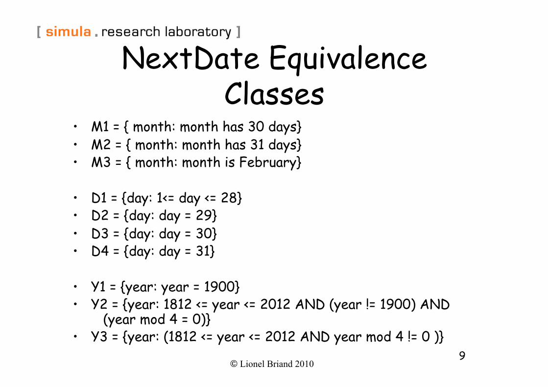
NextDate Equivalence Classes
• M1 = { month: month has 30 days} • M2 = { month: month has 31 days} • M3 = { month: month is February}
• D1 = {day: 1<= day <= 28} • D2 = {day: day = 29} • D3 = {day: day = 30} • D4 = {day: day = 31}
• Y1 = {year: year = 1900} • Y2 = {year: 1812 <= year <= 2012 AND (year != 1900) AND
(year mod 4 = 0)} • Y3 = {year: (1812 <= year <= 2012 AND year mod 4 != 0 )}
© Lionel Briand 2010 10
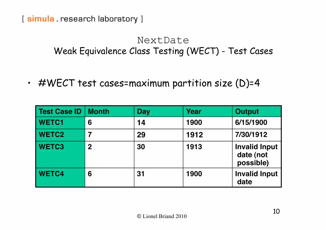
• #WECT test cases=maximum partition size (D)=4
Test Case ID! Month! Day! Year! Output!WETC1! 6! 14! 1900! 6/15/1900!WETC2! 7! 29! 1912! 7/30/1912!WETC3! 2! 30! 1913! Invalid Input
date (not possible)!
WETC4! 6! 31! 1900! Invalid Input date!
© Lionel Briand 2010 11
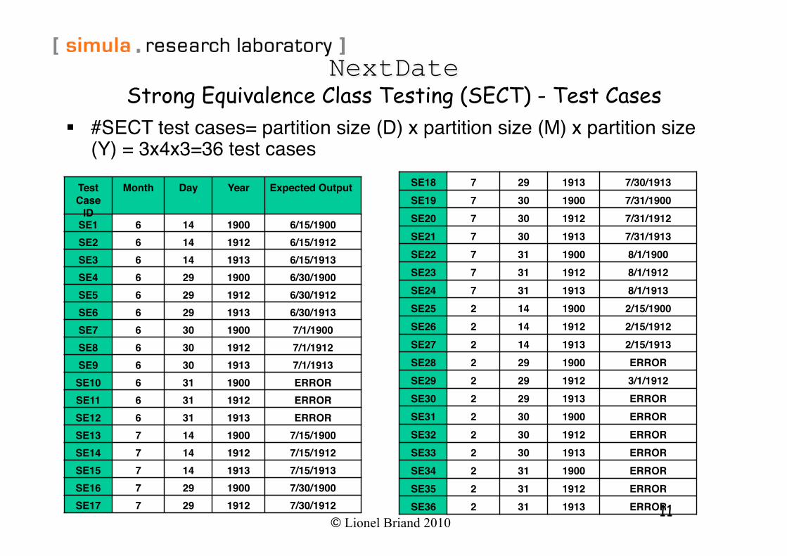
Test Case
ID!
Month! Day! Year! Expected Output!
SE1! 6! 14! 1900! 6/15/1900!SE2! 6! 14! 1912! 6/15/1912!SE3! 6! 14! 1913! 6/15/1913!SE4! 6! 29! 1900! 6/30/1900!SE5! 6! 29! 1912! 6/30/1912!SE6! 6! 29! 1913! 6/30/1913!SE7! 6! 30! 1900! 7/1/1900!SE8! 6! 30! 1912! 7/1/1912!SE9! 6! 30! 1913! 7/1/1913!
SE10! 6! 31! 1900! ERROR!SE11! 6! 31! 1912! ERROR!SE12! 6! 31! 1913! ERROR!SE13! 7! 14! 1900! 7/15/1900!SE14! 7! 14! 1912! 7/15/1912!SE15! 7! 14! 1913! 7/15/1913!SE16! 7! 29! 1900! 7/30/1900!SE17! 7! 29! 1912! 7/30/1912!
SE18! 7! 29! 1913! 7/30/1913!SE19! 7! 30! 1900! 7/31/1900!SE20! 7! 30! 1912! 7/31/1912!SE21! 7! 30! 1913! 7/31/1913!SE22! 7! 31! 1900! 8/1/1900!SE23! 7! 31! 1912! 8/1/1912!SE24! 7! 31! 1913! 8/1/1913!SE25! 2! 14! 1900! 2/15/1900!SE26! 2! 14! 1912! 2/15/1912!SE27! 2! 14! 1913! 2/15/1913!SE28! 2! 29! 1900! ERROR!SE29! 2! 29! 1912! 3/1/1912!SE30! 2! 29! 1913! ERROR!SE31! 2! 30! 1900! ERROR!SE32! 2! 30! 1912! ERROR!SE33! 2! 30! 1913! ERROR!SE34! 2! 31! 1900! ERROR!SE35! 2! 31! 1912! ERROR!SE36! 2! 31! 1913! ERROR!
#SECT test cases= partition size (D) x partition size (M) x partition size (Y) = 3x4x3=36 test cases"
© Lionel Briand 2010 12
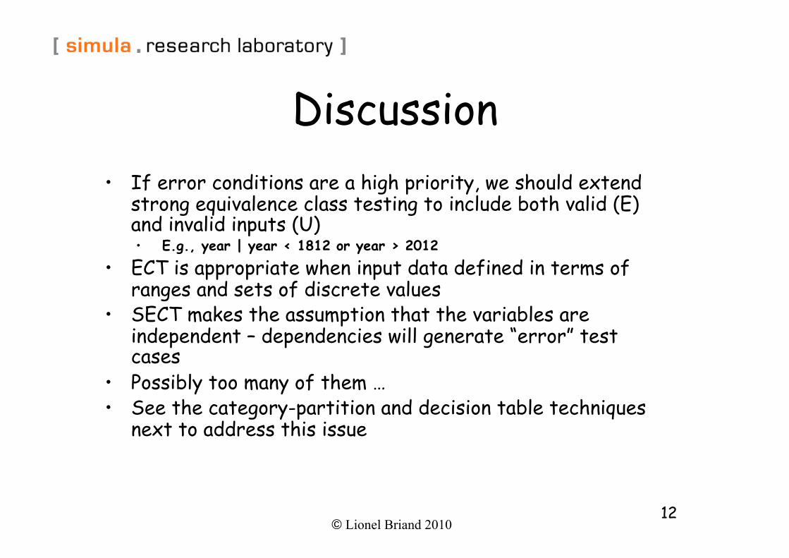
Discussion • If error conditions are a high priority, we should extend
strong equivalence class testing to include both valid (E) and invalid inputs (U) • E.g., year | year < 1812 or year > 2012
• ECT is appropriate when input data defined in terms of ranges and sets of discrete values
• SECT makes the assumption that the variables are independent – dependencies will generate “error” test cases
• Possibly too many of them … • See the category-partition and decision table techniques
next to address this issue

© Lionel Briand 2010 13
Boundary Value Testing
© Lionel Briand 2010 14
Motivations • We have partitioned input domains into
suitable classes, on the assumption that the behavior of the program is “similar”
• Some typical programming errors happen to be at the boundary between different classes
• This is what boundary value testing focuses on
• Simpler but complementary to previous techniques
© Lionel Briand 2010 15
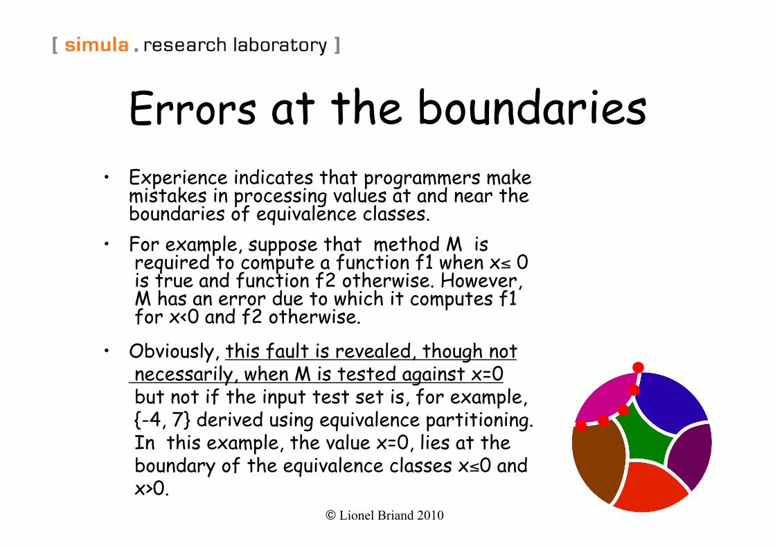
Errors at the boundaries • Experience indicates that programmers make
mistakes in processing values at and near the boundaries of equivalence classes.
• For example, suppose that method M is required to compute a function f1 when x≤ 0 is true and function f2 otherwise. However, M has an error due to which it computes f1 for x<0 and f2 otherwise.
• Obviously, this fault is revealed, though not necessarily, when M is tested against x=0 but not if the input test set is, for example, {-4, 7} derived using equivalence partitioning. In this example, the value x=0, lies at the boundary of the equivalence classes x≤0 and x>0.
© Lionel Briand 2010 16
Boundary Value Analysis • Boundary value analysis is a test selection
technique that targets faults in applications at the boundaries of equivalence classes.
• While equivalence partitioning selects tests from within equivalence classes, boundary value analysis focuses on tests at and near the boundaries of equivalence classes.
• Certainly, tests derived using either of the two techniques may overlap.
© Lionel Briand 2010 17
Example: 1. Create equivalence classes
Function findPrice() has two parameters: an item code must be in the range 99..999 and quantity in the range 1..100,
Equivalence classes for code: E1: Values less than 99. E2: Values in the range. E3: Values greater than 999.
Equivalence classes for qty: E4: Values less than 1. E5: Values in the range. E6: Values greater than 100.
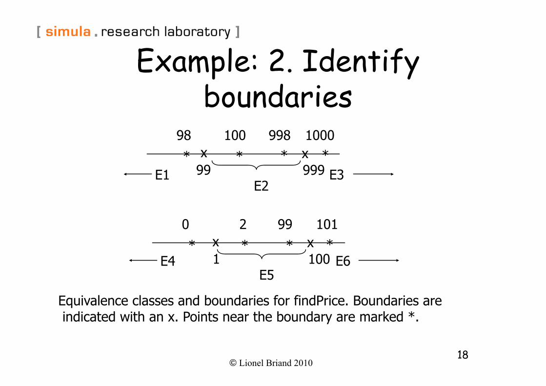
© Lionel Briand 2010 18
E1 E2
E3
98 100 998 1000
99 999 x x * * * *
Example: 2. Identify boundaries
Equivalence classes and boundaries for findPrice. Boundaries are indicated with an x. Points near the boundary are marked *.
E4 E5
E6
0 2 99 101
1 100 x x * * * *
© Lionel Briand 2010 19
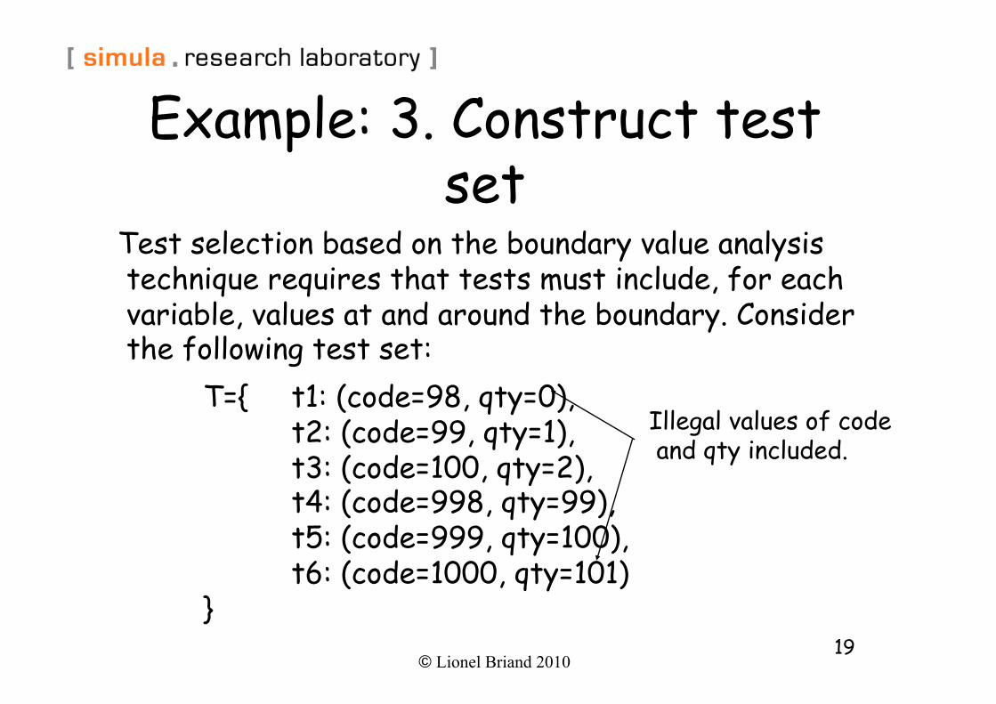
Example: 3. Construct test set
Test selection based on the boundary value analysis technique requires that tests must include, for each variable, values at and around the boundary. Consider the following test set:
T={ t1: (code=98, qty=0), t2: (code=99, qty=1), t3: (code=100, qty=2), t4: (code=998, qty=99), t5: (code=999, qty=100), t6: (code=1000, qty=101)
}
Illegal values of code and qty included.
© Lionel Briand 2010 20
Principles
• Input variable values (within a class) at their minimum, just above the minimum, a nominal value, just below their maximum, and at their maximum.
• Convention: min, min+, nom, max-, max • Hold the values of all but one variable
at their nominal values, letting one variable assume its extreme value
© Lionel Briand 2010 21
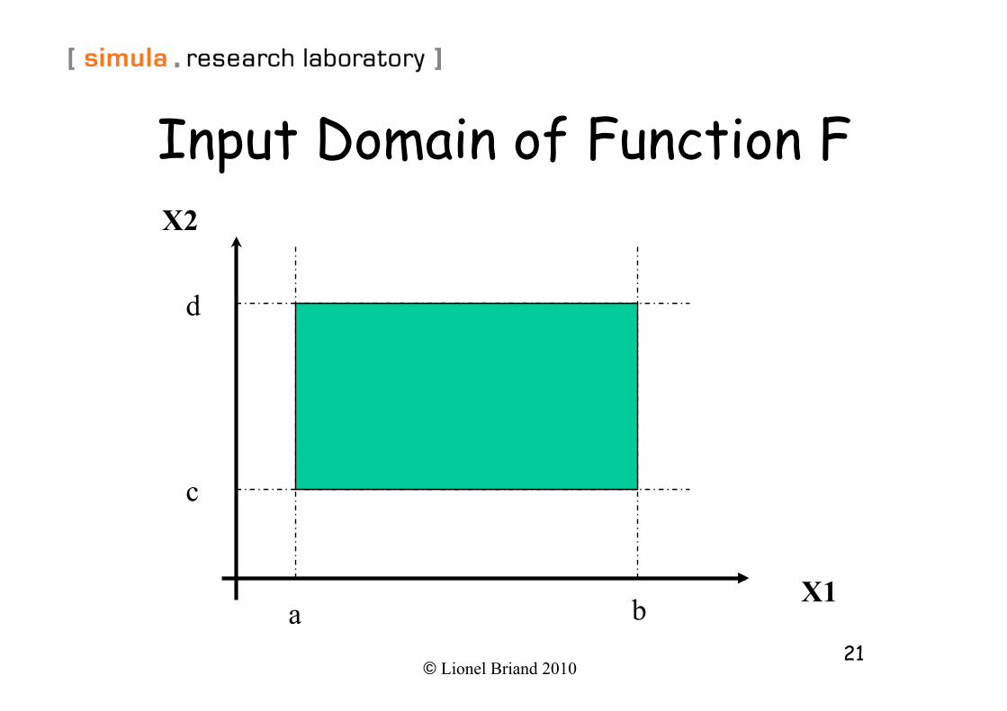
Input Domain of Function F
a b
d
c
X1
X2
© Lionel Briand 2010 22
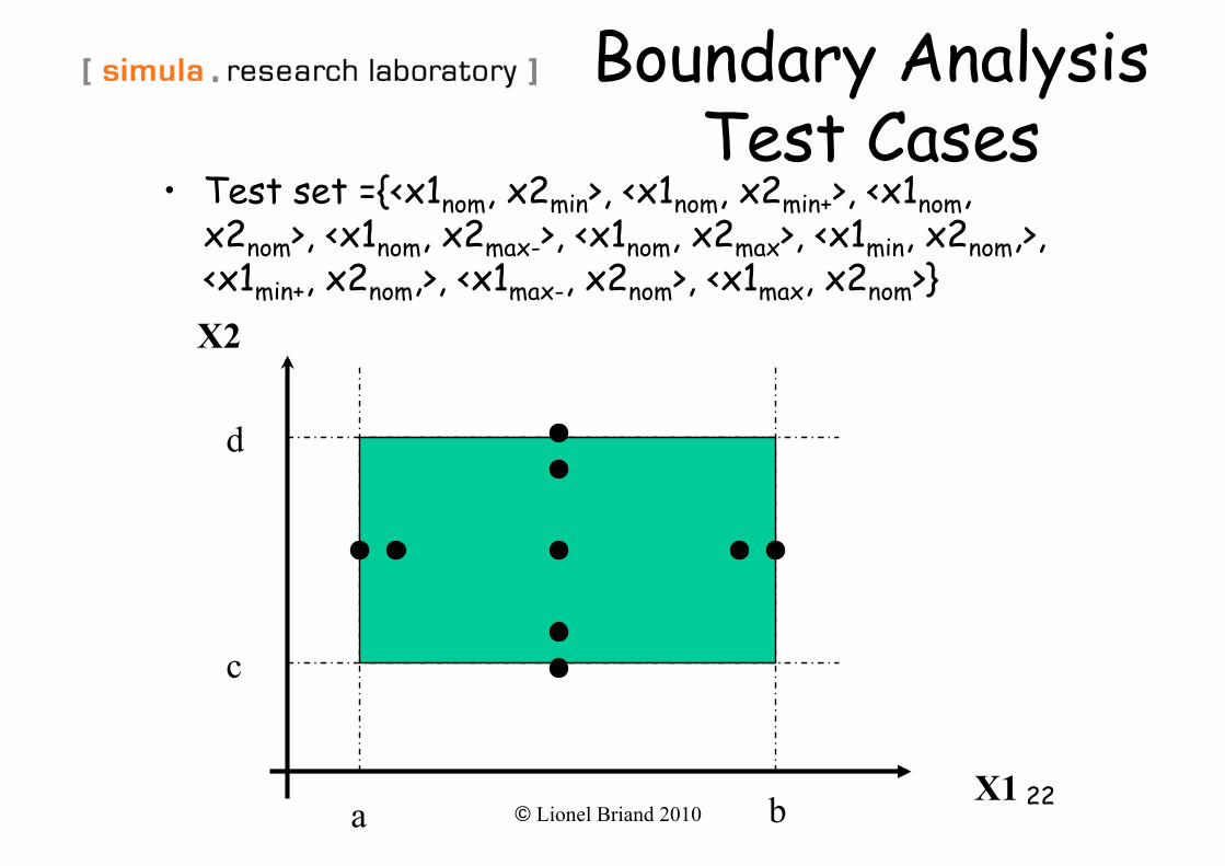
Boundary Analysis Test Cases
• Test set ={<x1nom, x2min>, <x1nom, x2min+>, <x1nom, x2nom>, <x1nom, x2max->, <x1nom, x2max>, <x1min, x2nom,>, <x1min+, x2nom,>, <x1max-, x2nom>, <x1max, x2nom>}
a b
d
c
X1
X2
© Lionel Briand 2010 23
General Case and Limitations
• A function with n variables will require 4n + 1 test cases
• Works well with variables that represent bounded physical quantities
• No consideration of the nature of the function and the meaning of variables
• Rudimentary technique that is amenable to robustness testing
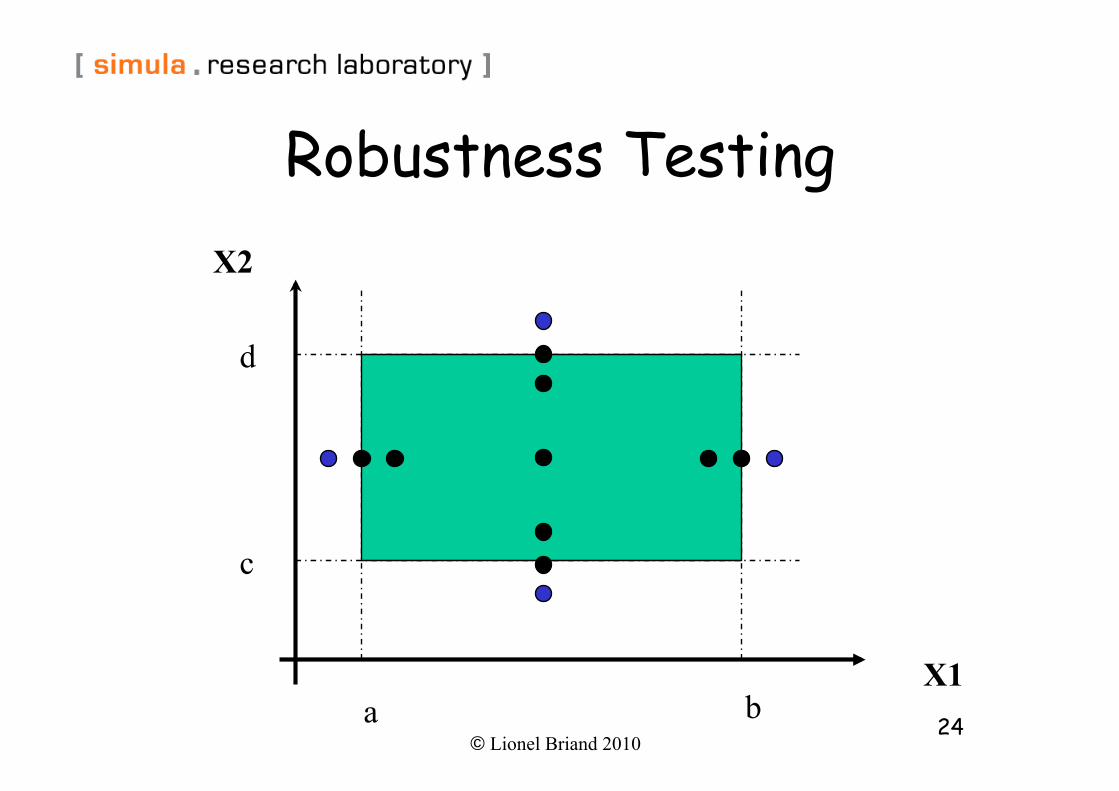
© Lionel Briand 2010 24
Robustness Testing
d
c
X1
X2
a b
© Lionel Briand 2010 25
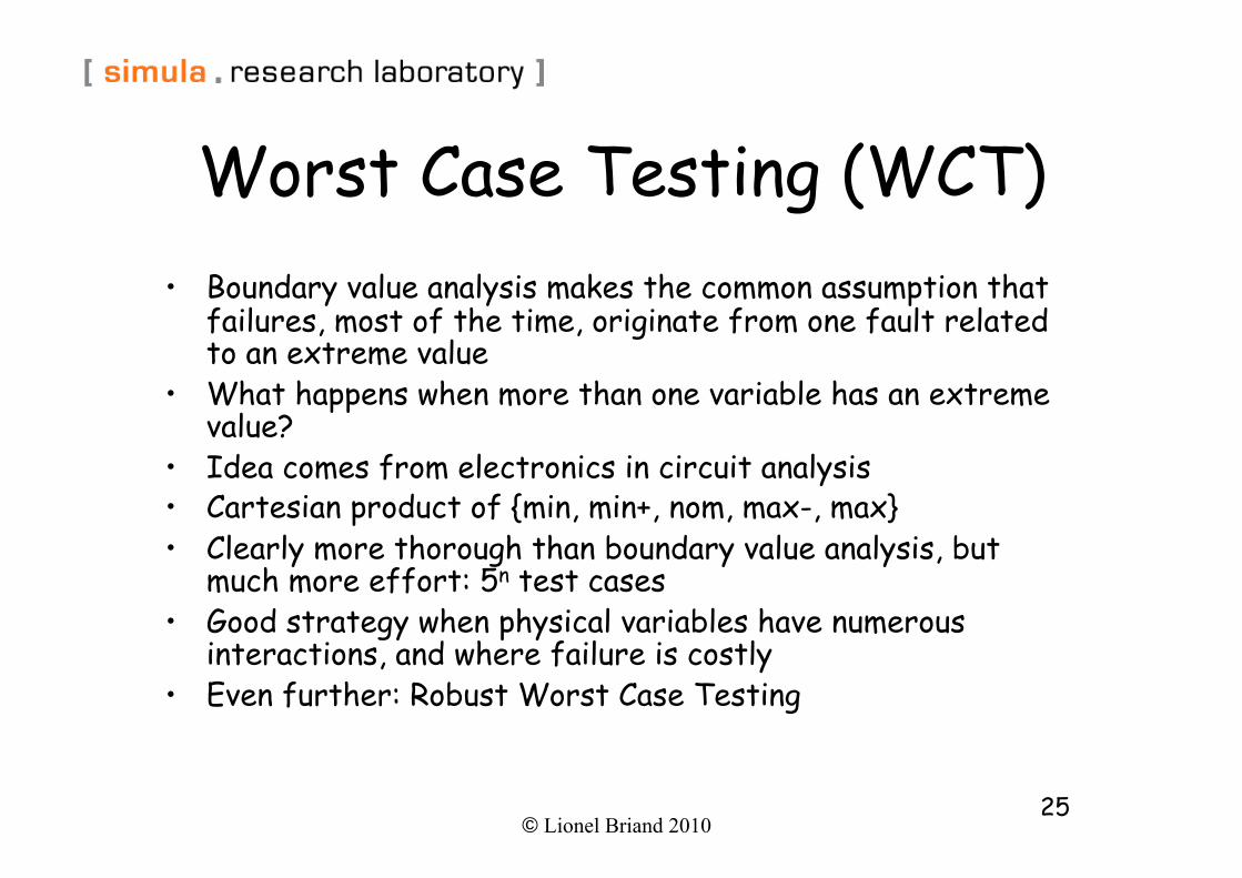
Worst Case Testing (WCT) • Boundary value analysis makes the common assumption that
failures, most of the time, originate from one fault related to an extreme value
• What happens when more than one variable has an extreme value?
• Idea comes from electronics in circuit analysis • Cartesian product of {min, min+, nom, max-, max} • Clearly more thorough than boundary value analysis, but
much more effort: 5n test cases • Good strategy when physical variables have numerous
interactions, and where failure is costly • Even further: Robust Worst Case Testing
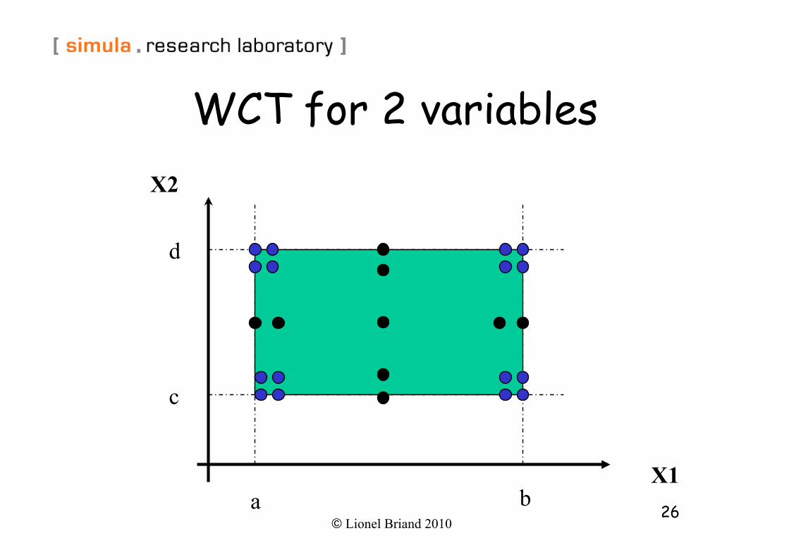
© Lionel Briand 2010 26
WCT for 2 variables
d
c
X1
X2
a b
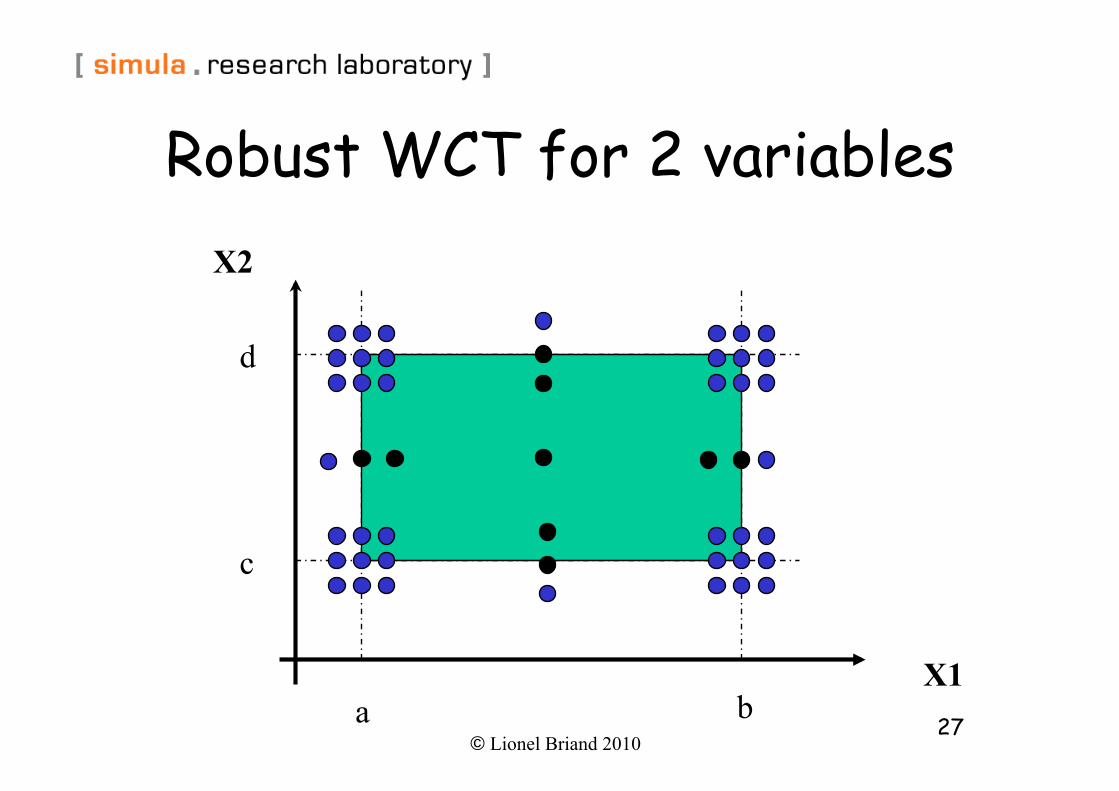
© Lionel Briand 2010 27
Robust WCT for 2 variables
d
c
X1
X2
a b
© Lionel Briand 2010 28
Category-Partition Testing
© Lionel Briand 2010 29
Steps • Extends and combine ECT, boundary value analysis. • The system is divided into individual “functions” (use cases)
that can be independently tested • The method identifies the parameters of each “function”
and, for each parameter, identifies distinct categories • Besides parameters, environment characteristics, under
which the function operates (characteristics of system state), can also be considered, e.g., versions of libraries.
• Categories are major properties or characteristics • The categories are further subdivided into choices in the
same way as equivalence partitioning is applied (value subdomains)
© Lionel Briand 2010 30
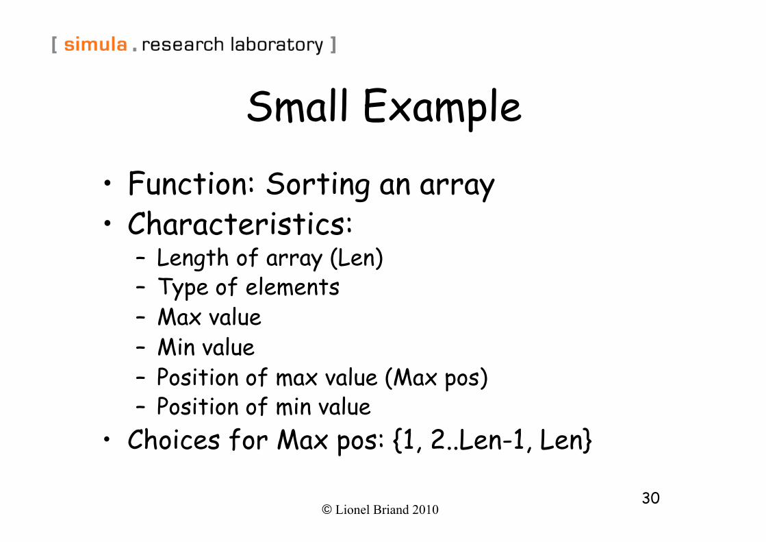
Small Example
• Function: Sorting an array • Characteristics:
– Length of array (Len) – Type of elements – Max value – Min value – Position of max value (Max pos) – Position of min value
• Choices for Max pos: {1, 2..Len-1, Len}
© Lionel Briand 2010 31
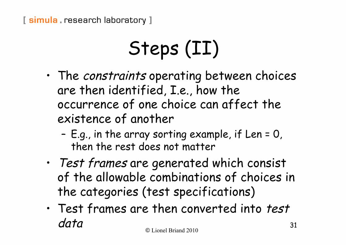
Steps (II) • The constraints operating between choices
are then identified, I.e., how the occurrence of one choice can affect the existence of another – E.g., in the array sorting example, if Len = 0,
then the rest does not matter • Test frames are generated which consist
of the allowable combinations of choices in the categories (test specifications)
• Test frames are then converted into test data
© Lionel Briand 2010 32
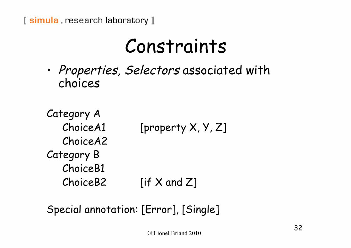
Constraints • Properties, Selectors associated with
choices
Category A ChoiceA1 [property X, Y, Z] ChoiceA2
Category B ChoiceB1 ChoiceB2 [if X and Z]
Special annotation: [Error], [Single]
© Lionel Briand 2010 33
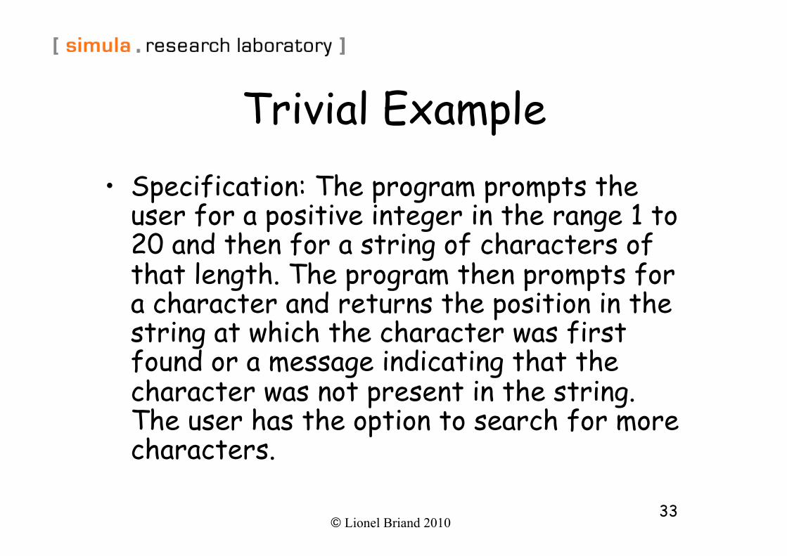
Trivial Example • Specification: The program prompts the
user for a positive integer in the range 1 to 20 and then for a string of characters of that length. The program then prompts for a character and returns the position in the string at which the character was first found or a message indicating that the character was not present in the string. The user has the option to search for more characters.
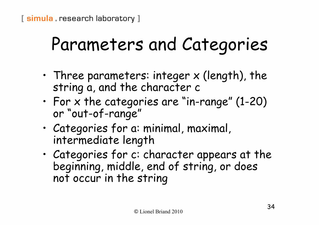
© Lionel Briand 2010 34
Parameters and Categories • Three parameters: integer x (length), the
string a, and the character c • For x the categories are “in-range” (1-20)
or “out-of-range” • Categories for a: minimal, maximal,
intermediate length • Categories for c: character appears at the
beginning, middle, end of string, or does not occur in the string
© Lionel Briand 2010 35
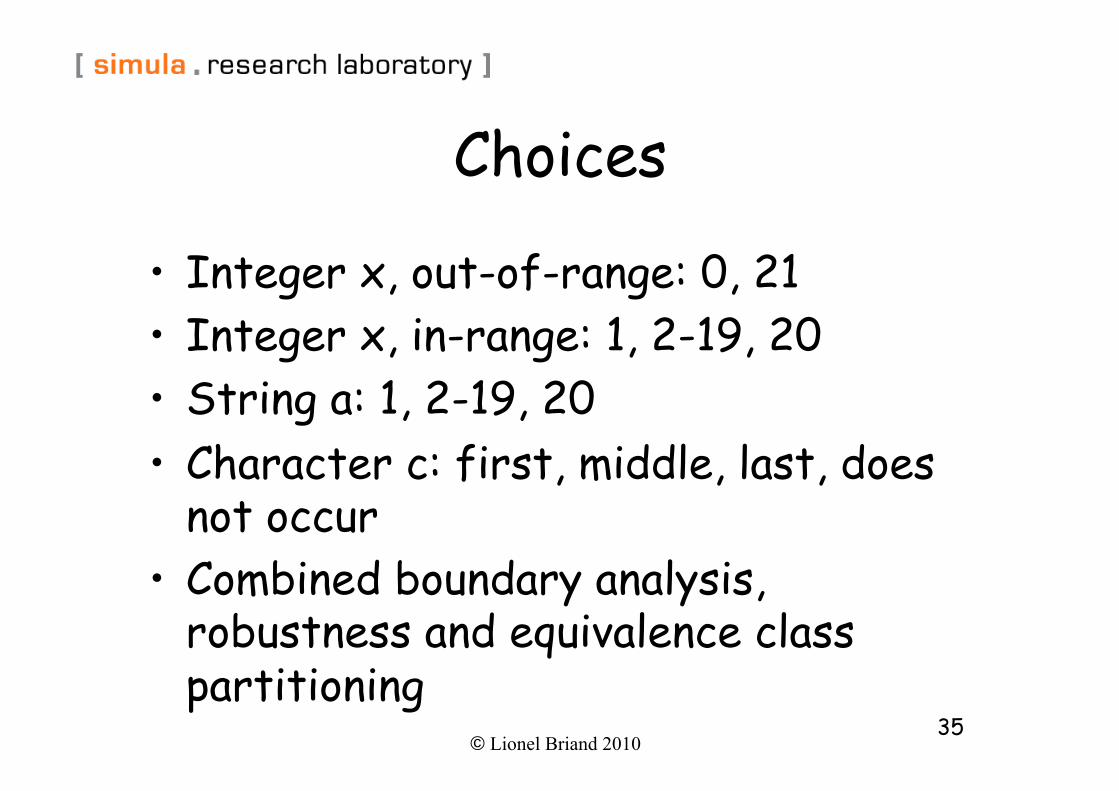
Choices
• Integer x, out-of-range: 0, 21 • Integer x, in-range: 1, 2-19, 20 • String a: 1, 2-19, 20 • Character c: first, middle, last, does
not occur • Combined boundary analysis,
robustness and equivalence class partitioning
© Lionel Briand 2010 36
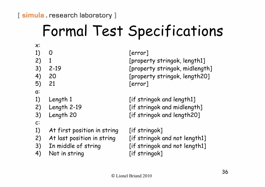
Formal Test Specifications x: 1) 0 [error] 2) 1 [property stringok, length1] 3) 2-19 [property stringok, midlength] 4) 20 [property stringok, length20] 5) 21 [error] a: 1) Length 1 [if stringok and length1] 2) Length 2-19 [if stringok and midlength] 3) Length 20 [if stringok and length20] c: 1) At first position in string [if stringok] 2) At last position in string [if stringok and not length1] 3) In middle of string [if stringok and not length1] 4) Not in string [if stringok]
© Lionel Briand 2010 37
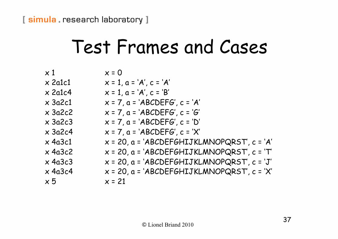
Test Frames and Cases x 1 x = 0 x 2a1c1 x = 1, a = ‘A’, c = ‘A’ x 2a1c4 x = 1, a = ‘A’, c = ‘B’ x 3a2c1 x = 7, a = ‘ABCDEFG’, c = ‘A’ x 3a2c2 x = 7, a = ‘ABCDEFG’, c = ‘G’ x 3a2c3 x = 7, a = ‘ABCDEFG’, c = ‘D’ x 3a2c4 x = 7, a = ‘ABCDEFG’, c = ‘X’ x 4a3c1 x = 20, a = ‘ABCDEFGHIJKLMNOPQRST’, c = ‘A’ x 4a3c2 x = 20, a = ‘ABCDEFGHIJKLMNOPQRST’, c = ‘T’ x 4a3c3 x = 20, a = ‘ABCDEFGHIJKLMNOPQRST’, c = ‘J’ x 4a3c4 x = 20, a = ‘ABCDEFGHIJKLMNOPQRST’, c = ‘X’ x 5 x = 21
© Lionel Briand 2010 38
Criteria Using Choices • All Combinations (AC): This is what was shown in the previous
example, what is typically done when using category-partition. One value for every choice of every parameter must be used with one value of every (possible) choice of every other category.
• Each choice (EC): This is a weaker criterion. One value from each choice for each category must be used at least in one test case.
• Base Choice (BC): This criterion is a compromise. A base choice is chosen for each category, and a first base test is formed by using the base choice for each category. Subsequent tests are chosen by holding all but one base choice constant (I.e., we select a non-base choice for one category) and forming choice combinations by covering all non-base choices of the selected category. This procedure is repeated for each category.
• The base choice can be the simplest, smallest, first in some ordering, or most likely from an end-user point of view, e.g., in the previous example, character c occurs in the middle of the string, length x is within 2-19.
© Lionel Briand 2010 39
Conclusions • Identifying parameters and environments
conditions, and categories, is heavily relying on the experience of the tester
• Makes testing decisions explicit (e.g., constraints), open for review
• Combine boundary analysis, robustness testing, and equivalence class partitioning
• Once the first step is completed, the technique is straightforward and can be automated
• Techniques for test case reduction makes it useful for practical testing
© Lionel Briand 2010 40
Decision Tables
© Lionel Briand 2010 41
Motivations • Help express test requirements in a directly
usable form • Easy to understand and support the systematic
derivation of tests • Support automated or manual generation of test
cases • A particular response or response subset is to be
selected by evaluating many related conditions • Ideal for describing situations in which a number
of combinations of actions are taken under varying sets of conditions, e.g., control systems
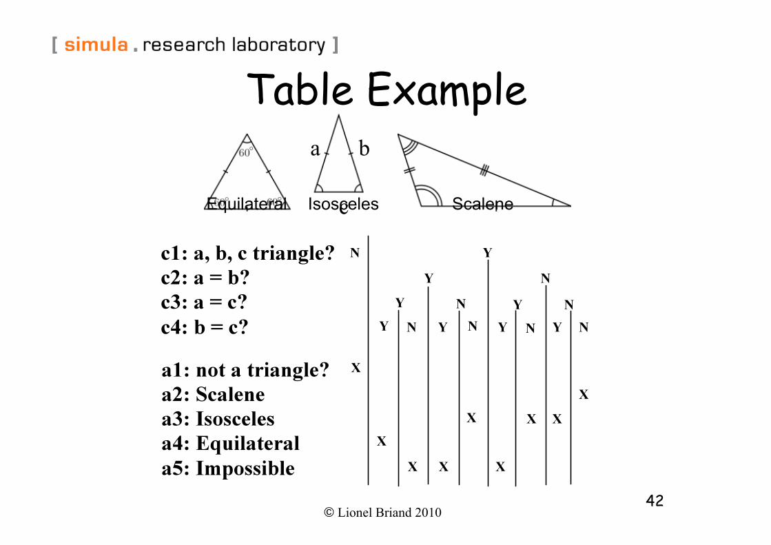
© Lionel Briand 2010 42
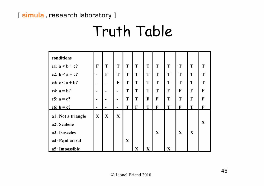
Table Example
Equilateral Isosceles Scalene
a b
c
© Lionel Briand 2010 43
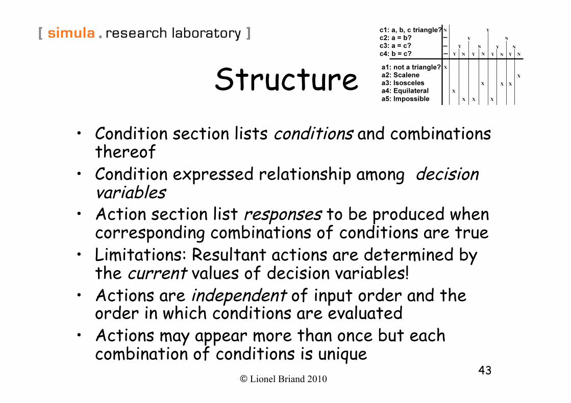
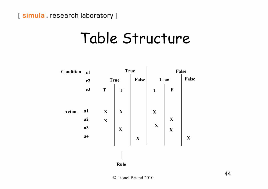
Structure • Condition section lists conditions and combinations
thereof • Condition expressed relationship among decision
variables • Action section list responses to be produced when
corresponding combinations of conditions are true • Limitations: Resultant actions are determined by
the current values of decision variables! • Actions are independent of input order and the
order in which conditions are evaluated • Actions may appear more than once but each
combination of conditions is unique
© Lionel Briand 2010 44
Table Structure
© Lionel Briand 2010 45
Truth Table
© Lionel Briand 2010 46
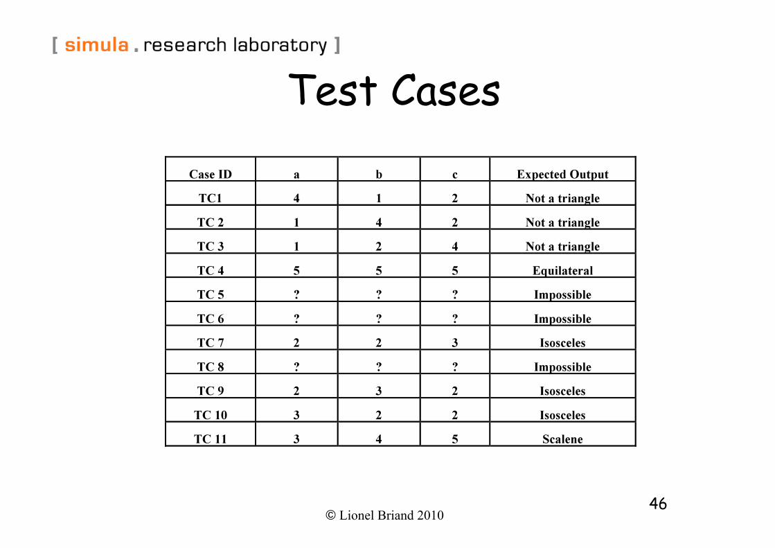
Test Cases
© Lionel Briand 2010 47
Ideal Usage Conditions • One of several distinct responses is to be selected
according to distinct cases of input variables • These cases can be modeled by mutually exclusive
Boolean expressions on the input variables • The response to be produced does not depend on
the order in which input variables are set or evaluated (e.g., events are received)
• The response does not depend on prior inputs or outputs
© Lionel Briand 2010 48
Scale • For n conditions, there may be at most 2n variants
(unique combinations of conditions and actions) • But, fortunately, there are usually much fewer
explicit variants … • “Don’t care” values in decision tables help reduce
the number of variants • “Don’t care” can correspond to several cases:
– The inputs are necessary but have no effect – The inputs may be omitted – Mutually exclusive cases (type-safe exclusions)
© Lionel Briand 2010 49
Special Cases • “can’t happen” : reflect some assumption that some
inputs are mutually exclusive, or that they cannot be produced in the environment.
• A chronic source of bugs, e.g., Ariane 5 • “can’t happen” do occur because of programming
errors and unexpected change effects • “don’t know” condition reflect an incomplete model,
e.g., due to incomplete documentation • Most of the time, they are specification bugs
© Lionel Briand 2010 50
Cause-Effect Graphs
© Lionel Briand 2010 51
Definition • Graphical technique that helps derive decision
tables • Aim at supporting interaction with domain experts
and the reverse engineering of specifications, for the purpose of testing.
• Identify causes (conditions on inputs, stimuli) and effects (outputs, changes in system state)
• Causes have to be stated in such a way to be either true or false (Boolean expression)
• Specifies explicitly (environmental, external) constraints on causes and effects
• Help select more “significant” subset of input-output combinations and build smaller decision tables
© Lionel Briand 2010 52
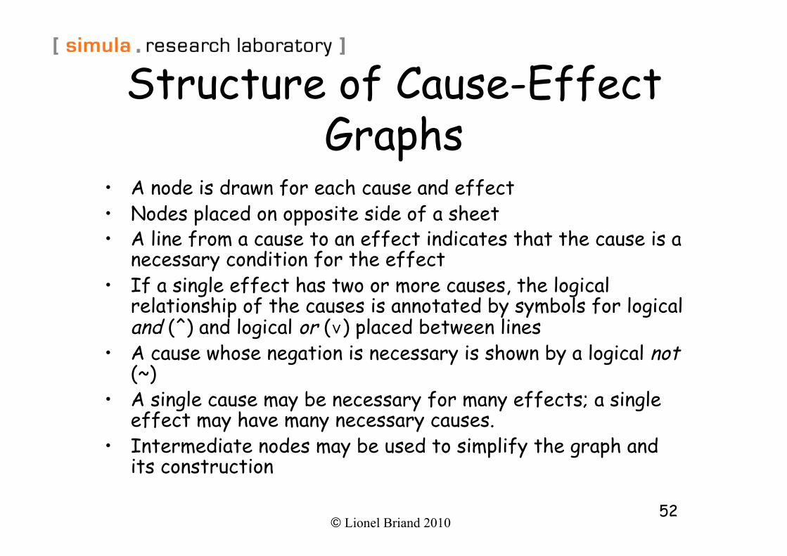
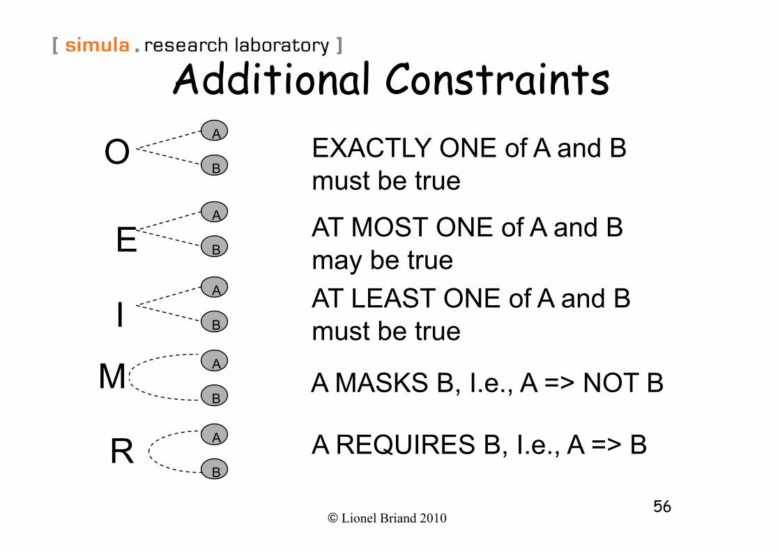
Structure of Cause-Effect Graphs
• A node is drawn for each cause and effect • Nodes placed on opposite side of a sheet • A line from a cause to an effect indicates that the cause is a
necessary condition for the effect • If a single effect has two or more causes, the logical
relationship of the causes is annotated by symbols for logical and (^) and logical or (∨) placed between lines
• A cause whose negation is necessary is shown by a logical not (~)
• A single cause may be necessary for many effects; a single effect may have many necessary causes.
• Intermediate nodes may be used to simplify the graph and its construction
© Lionel Briand 2010 53
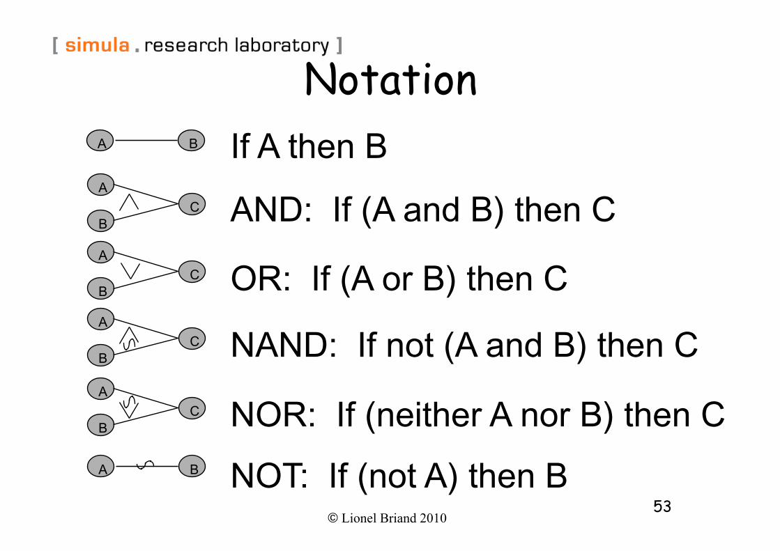
Notation
B A
C
A
B
C
A
B
C
A
B
C
A
B
B A If A then B
AND: If (A and B) then C
OR: If (A or B) then C
NAND: If not (A and B) then C
NOR: If (neither A nor B) then C
NOT: If (not A) then B
© Lionel Briand 2010 54
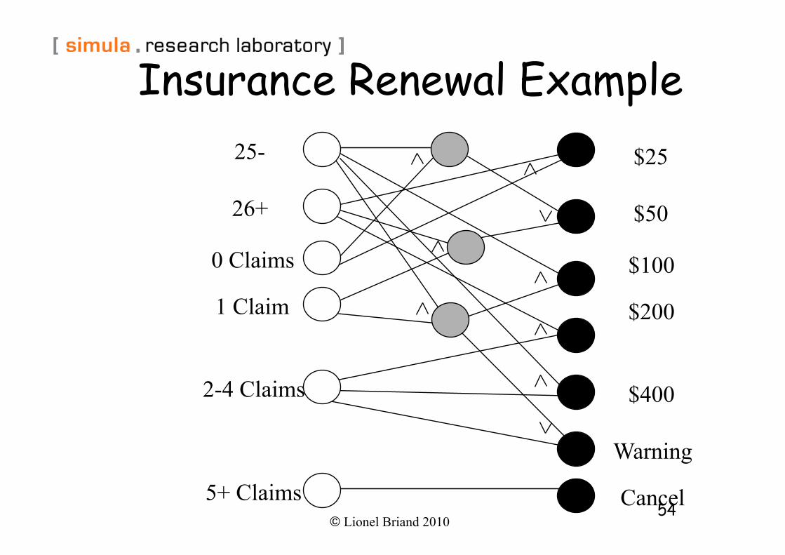
Insurance Renewal Example 25-
26+
0 Claims
1 Claim
2-4 Claims
5+ Claims
$25
$50
$100
$200
$400
Cancel
Warning
© Lionel Briand 2010 55
Another Table Example Insurance Renewal
Condition Section Action Section
Variant Claims Age Premium Increase $
Send Warning
Cancel
1 0 25- 50 No No
2 0 26+ 25 No No
3 1 25- 100 Yes No
4 1 26+ 50 No No
5 2 to 4 25- 400 Yes No
6 2 to 4 26+ 200 Yes No
7 5+ Any 0 No Yes
© Lionel Briand 2010 56
Additional Constraints A
B
A
B E A
B I A
B M
A
B
EXACTLY ONE of A and B must be true
AT MOST ONE of A and B may be true
AT LEAST ONE of A and B must be true
A MASKS B, I.e., A => NOT B
A REQUIRES B, I.e., A => B R
O
© Lionel Briand 2010 57
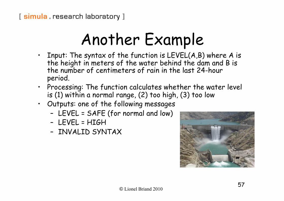
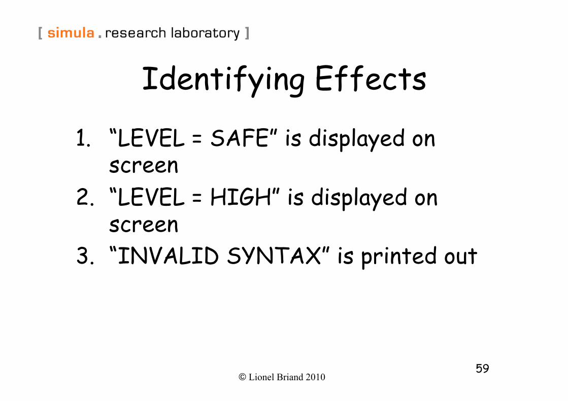
Another Example • Input: The syntax of the function is LEVEL(A,B) where A is
the height in meters of the water behind the dam and B is the number of centimeters of rain in the last 24-hour period.
• Processing: The function calculates whether the water level is (1) within a normal range, (2) too high, (3) too low
• Outputs: one of the following messages – LEVEL = SAFE (for normal and low) – LEVEL = HIGH – INVALID SYNTAX
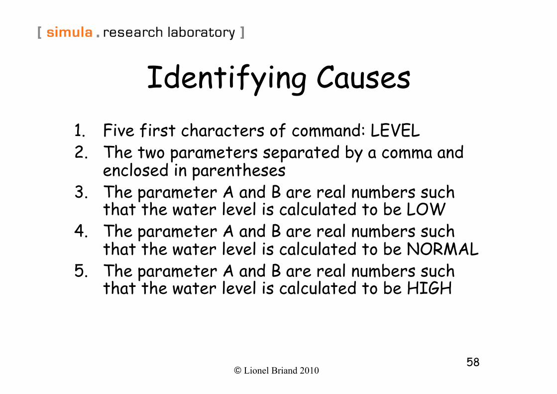
© Lionel Briand 2010 58
Identifying Causes 1. Five first characters of command: LEVEL 2. The two parameters separated by a comma and
enclosed in parentheses 3. The parameter A and B are real numbers such
that the water level is calculated to be LOW 4. The parameter A and B are real numbers such
that the water level is calculated to be NORMAL 5. The parameter A and B are real numbers such
that the water level is calculated to be HIGH
© Lionel Briand 2010 59
Identifying Effects
1. “LEVEL = SAFE” is displayed on screen
2. “LEVEL = HIGH” is displayed on screen
3. “INVALID SYNTAX” is printed out
© Lionel Briand 2010 60
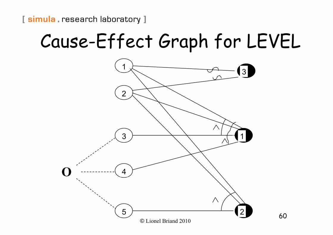
Cause-Effect Graph for LEVEL 3
4
1
2
1 3
2 5
O
© Lionel Briand 2010 61
Deriving a Decision Table • A row for each cause or effect • The columns correspond to test cases (variants) • Examine each effect and listing all combinations
(conjunctions) of causes (subject to constraints) that can lead to that effect
• Create a column for each possible combination of causes
• For each combination, determine the state of other effects
• Two separate lines flow into effect E3, each corresponding to a test case, four lines flow into E1 but correspond to only two combinations
© Lionel Briand 2010 62
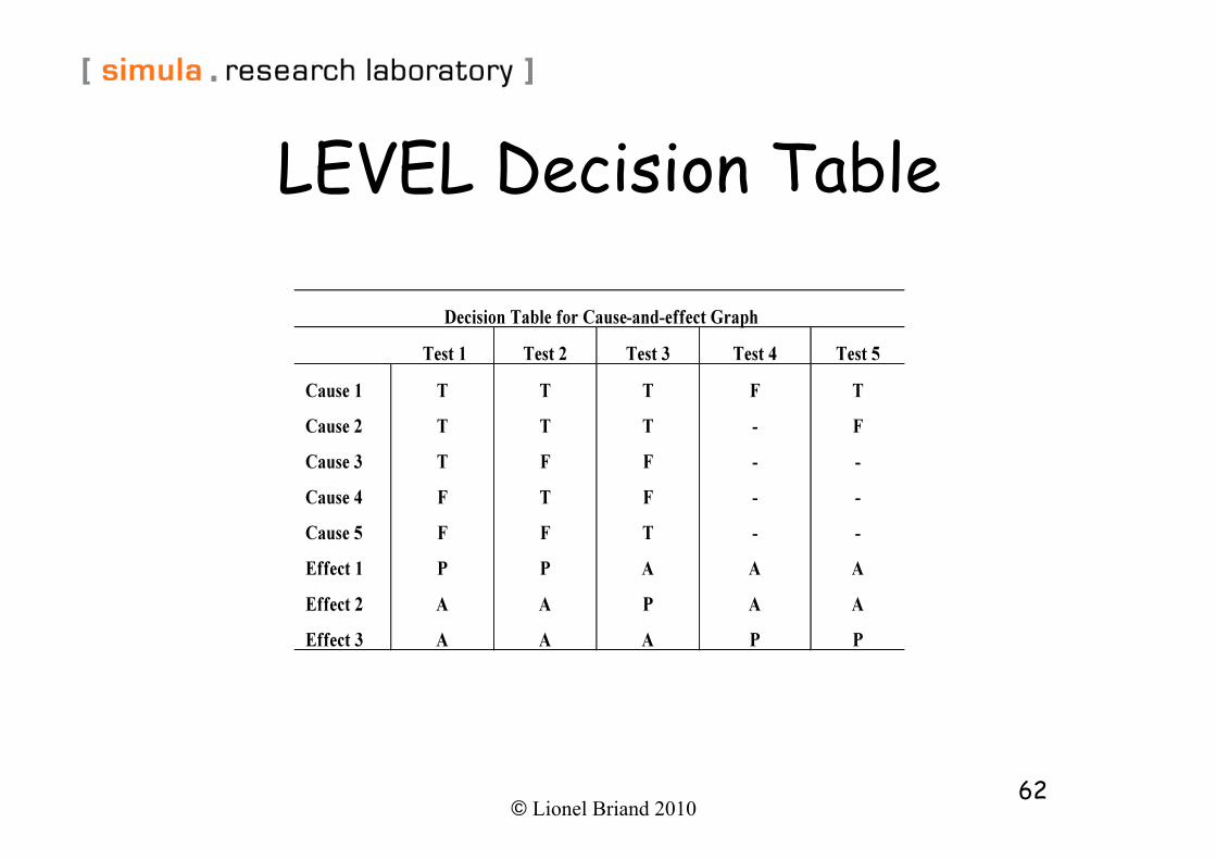
LEVEL Decision Table
© Lionel Briand 2010 63
Process • The specification is divided into workable
pieces • The causes and effects are identified from
the specification • Causes are linked to effects • The graph is annotated with constraints
describing impossible combinations of causes and/or effects
• The graph is used to generate a limited-entry decision table
• The columns of the table are converted into test cases
© Lionel Briand 2010 64
Discussion • Aids in selecting , in a systematic way, a high yield of test
cases • The cause-Effect graph can be used to identify all possible
combinations of causes and checking whether the effect corresponds to the specification
• It provides a test oracle and specifies constraints on outputs (effects), helping detecting wrong system states and output/action combinations
• If the graph is too large, for each admissible combination of effects, find some combinations of causes that cause that combination of effects by tracing back through the graph
• Because of additional constraints on graph, can be more restrictive than straight decision tables
• A beneficial side effect is that it points out incompleteness and ambiguities in the specifications
© Lionel Briand 2010 65
Testing Logic Functions or Predicates
© Lionel Briand 2010 66
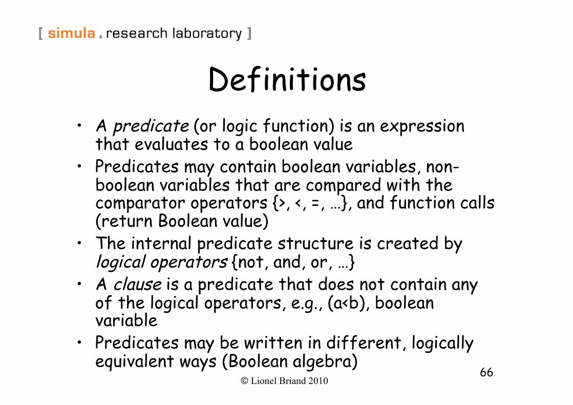
Definitions • A predicate (or logic function) is an expression
that evaluates to a boolean value • Predicates may contain boolean variables, non-
boolean variables that are compared with the comparator operators {>, <, =, …}, and function calls (return Boolean value)
• The internal predicate structure is created by logical operators {not, and, or, …}
• A clause is a predicate that does not contain any of the logical operators, e.g., (a<b), boolean variable
• Predicates may be written in different, logically equivalent ways (Boolean algebra)
© Lionel Briand 2010 67
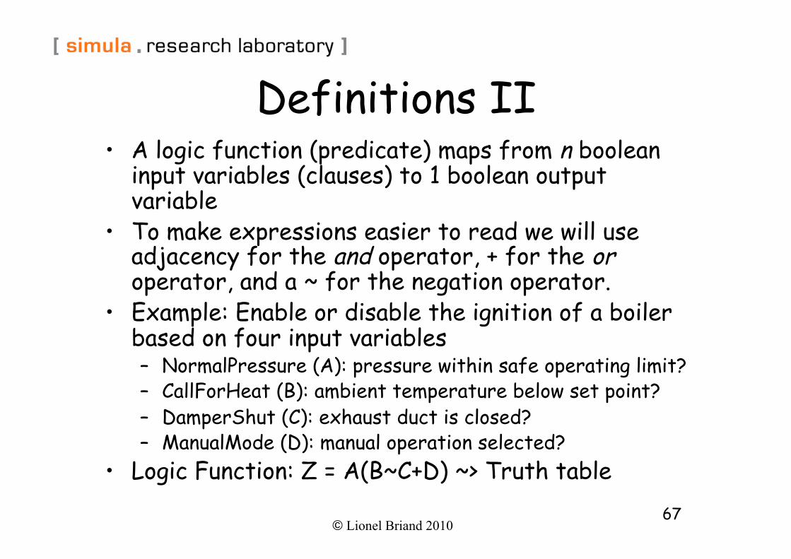
Definitions II • A logic function (predicate) maps from n boolean
input variables (clauses) to 1 boolean output variable
• To make expressions easier to read we will use adjacency for the and operator, + for the or operator, and a ~ for the negation operator.
• Example: Enable or disable the ignition of a boiler based on four input variables – NormalPressure (A): pressure within safe operating limit? – CallForHeat (B): ambient temperature below set point? – DamperShut (C): exhaust duct is closed? – ManualMode (D): manual operation selected?
• Logic Function: Z = A(B~C+D) ~> Truth table
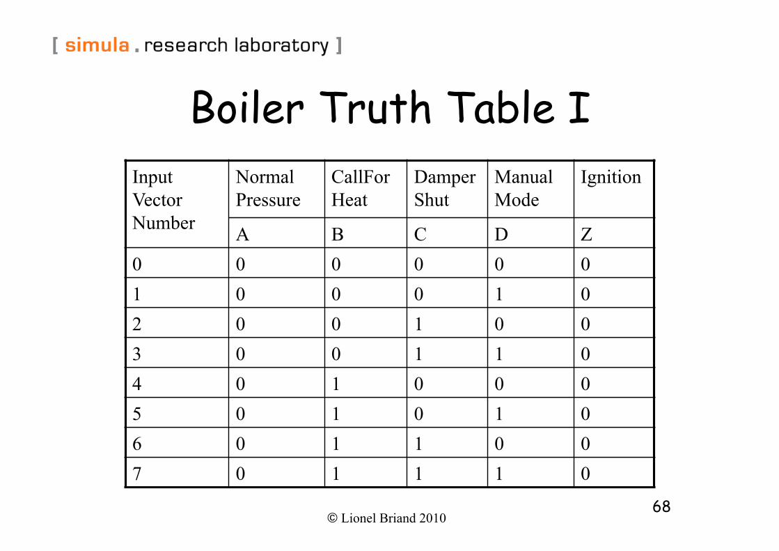
© Lionel Briand 2010 68
Boiler Truth Table I Input Vector Number
Normal Pressure
CallForHeat
DamperShut
ManualMode
Ignition
A B C D Z 0 0 0 0 0 0 1 0 0 0 1 0 2 0 0 1 0 0 3 0 0 1 1 0 4 0 1 0 0 0 5 0 1 0 1 0 6 0 1 1 0 0 7 0 1 1 1 0
© Lionel Briand 2010 69
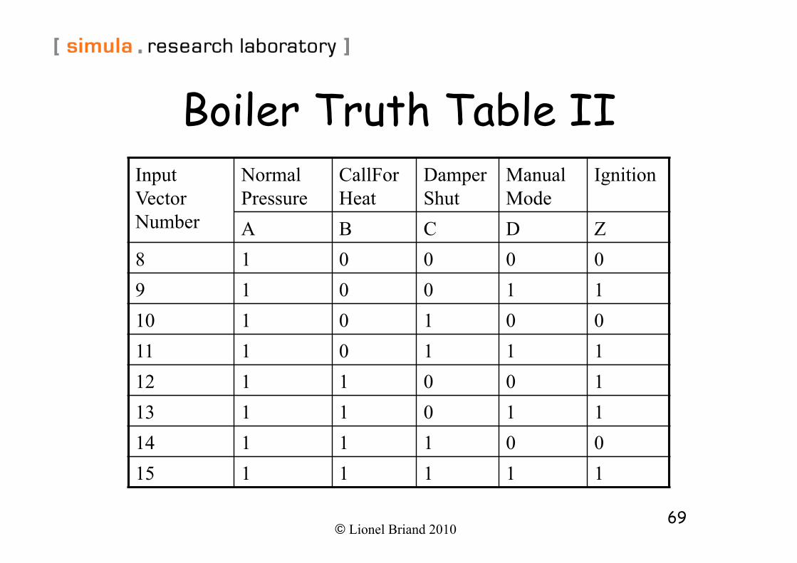
Boiler Truth Table II Input Vector Number
Normal Pressure
CallForHeat
DamperShut
ManualMode
Ignition
A B C D Z 8 1 0 0 0 0 9 1 0 0 1 1 10 1 0 1 0 0 11 1 0 1 1 1 12 1 1 0 0 1 13 1 1 0 1 1 14 1 1 1 0 0 15 1 1 1 1 1
© Lionel Briand 2010 70
Elements of Boolean Expressions • Boolean space: The n-dimensional space formed by
the input variables • Product term or conjunctive clause: String of
clauses related by the and operator • Sum-of-products or disjunctive normal form
(DNF): Product terms related by the or operator • Implicant: Each term of a sum-of-products
expression – sufficient condition to fulfill for True output of that expression
• Prime implicants: An implicant such that no subset (proper subterm) is also an implicant
• Logic minimization: Deriving compact (irredundant) but equivalent boolean expressions, using boolean algebra
© Lionel Briand 2010 71
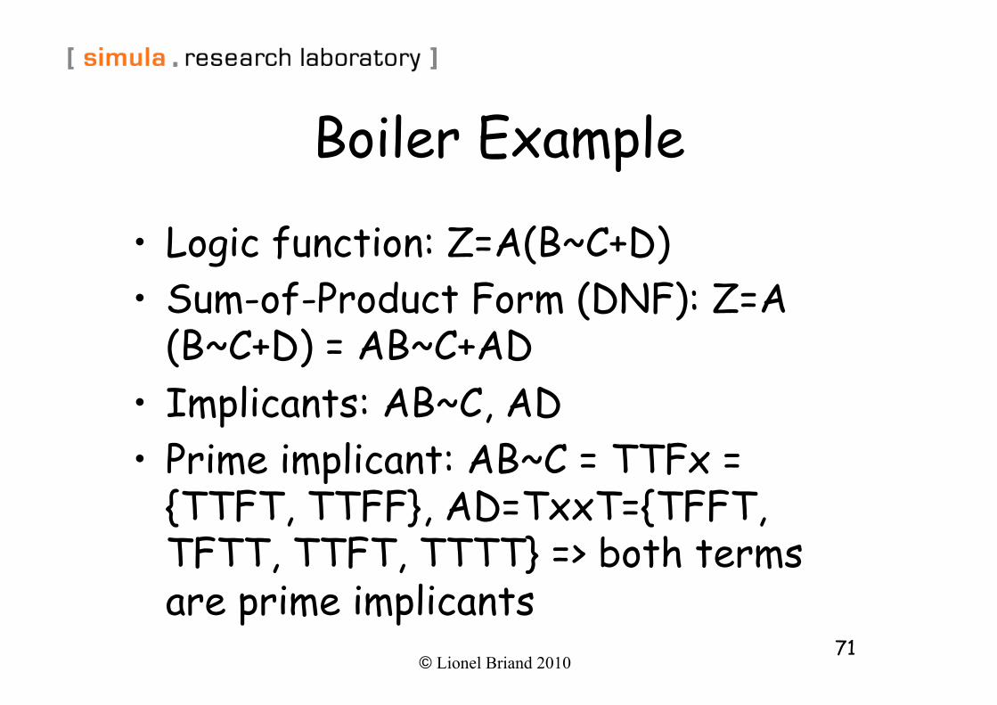
Boiler Example
• Logic function: Z=A(B~C+D) • Sum-of-Product Form (DNF): Z=A
(B~C+D) = AB~C+AD • Implicants: AB~C, AD • Prime implicant: AB~C = TTFx =
{TTFT, TTFF}, AD=TxxT={TFFT, TFTT, TTFT, TTTT} => both terms are prime implicants
© Lionel Briand 2010 72
From Graph to Logic Function
• Once a cause-effect graph is reviewed and considered correct, we want to derive a logic function for the purpose of deriving test requirements (in the form of a decision table)
• One function (predicate, truth table) exists for each effect (output variable)
• If several effects are present, then the resulting decision table is a composite of several truth tables that happen to share decision/input variables and actions/effects
• Easier to derive a function for each effect separately • Derive a Boolean function from the graph in a systematic
way
© Lionel Briand 2010 73
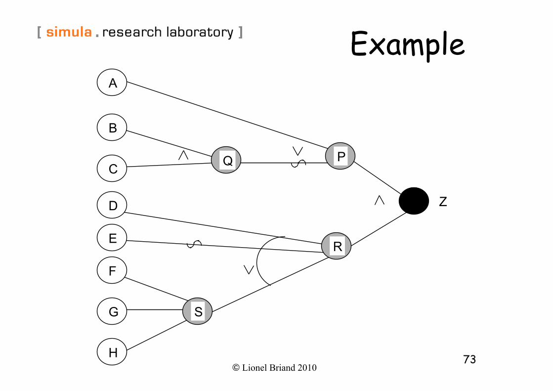
Example A
B
C
D
E
F
G
H
Q
S
R
P
Z
© Lionel Briand 2010 74
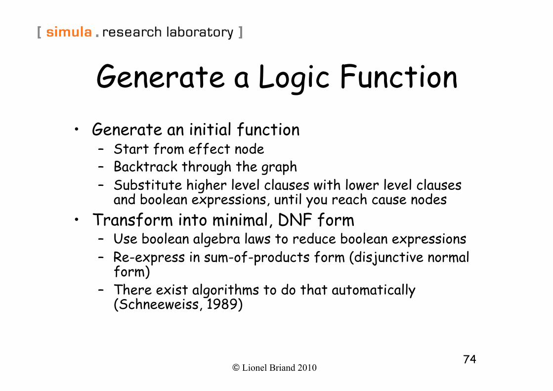
Generate a Logic Function • Generate an initial function
– Start from effect node – Backtrack through the graph – Substitute higher level clauses with lower level clauses
and boolean expressions, until you reach cause nodes • Transform into minimal, DNF form
– Use boolean algebra laws to reduce boolean expressions – Re-express in sum-of-products form (disjunctive normal
form) – There exist algorithms to do that automatically
(Schneeweiss, 1989)
© Lionel Briand 2010 75
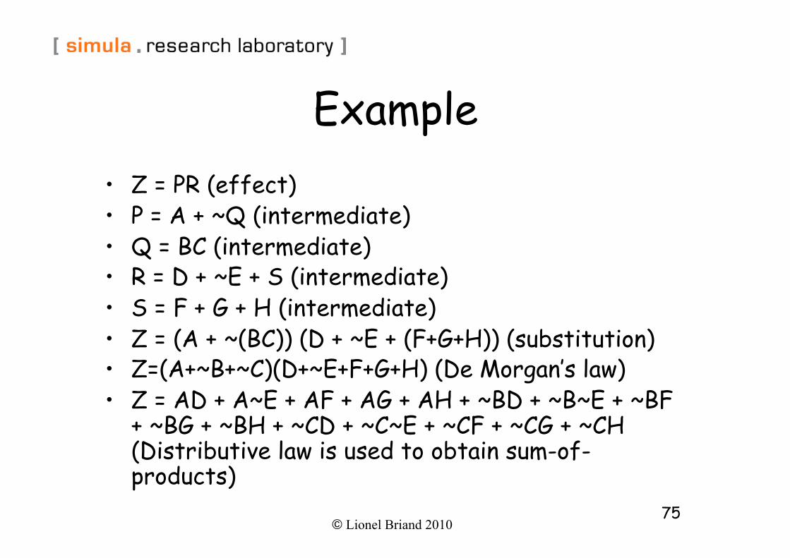
Example • Z = PR (effect) • P = A + ~Q (intermediate) • Q = BC (intermediate) • R = D + ~E + S (intermediate) • S = F + G + H (intermediate) • Z = (A + ~(BC)) (D + ~E + (F+G+H)) (substitution) • Z=(A+~B+~C)(D+~E+F+G+H) (De Morgan’s law) • Z = AD + A~E + AF + AG + AH + ~BD + ~B~E + ~BF
+ ~BG + ~BH + ~CD + ~C~E + ~CF + ~CG + ~CH (Distributive law is used to obtain sum-of-products)
© Lionel Briand 2010 76
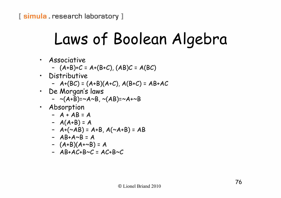
Laws of Boolean Algebra • Associative
– (A+B)+C = A+(B+C), (AB)C = A(BC) • Distributive
– A+(BC) = (A+B)(A+C), A(B+C) = AB+AC • De Morgan’s laws
– ~(A+B)=~A~B, ~(AB)=~A+~B • Absorption
– A + AB = A – A(A+B) = A – A+(~AB) = A+B, A(~A+B) = AB – AB+A~B = A – (A+B)(A+~B) = A – AB+AC+B~C = AC+B~C
© Lionel Briand 2010 77
Fault Model for Logic-based Testing
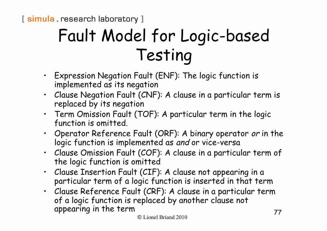
• Expression Negation Fault (ENF): The logic function is implemented as its negation
• Clause Negation Fault (CNF): A clause in a particular term is replaced by its negation
• Term Omission Fault (TOF): A particular term in the logic function is omitted.
• Operator Reference Fault (ORF): A binary operator or in the logic function is implemented as and or vice-versa
• Clause Omission Fault (COF): A clause in a particular term of the logic function is omitted
• Clause Insertion Fault (CIF): A clause not appearing in a particular term of a logic function is inserted in that term
• Clause Reference Fault (CRF): A clause in a particular term of a logic function is replaced by another clause not appearing in the term
© Lionel Briand 2010 78
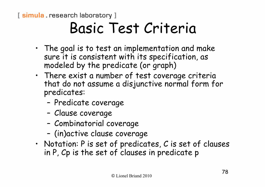
Basic Test Criteria • The goal is to test an implementation and make
sure it is consistent with its specification, as modeled by the predicate (or graph)
• There exist a number of test coverage criteria that do not assume a disjunctive normal form for predicates: – Predicate coverage – Clause coverage – Combinatorial coverage – (in)active clause coverage
• Notation: P is set of predicates, C is set of clauses in P, Cp is the set of clauses in predicate p
© Lionel Briand 2010 79
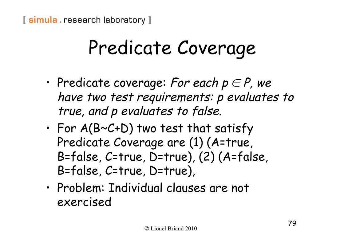
Predicate Coverage • Predicate coverage: For each p ∈ P, we
have two test requirements: p evaluates to true, and p evaluates to false.
• For A(B~C+D) two test that satisfy Predicate Coverage are (1) (A=true, B=false, C=true, D=true), (2) (A=false, B=false, C=true, D=true),
• Problem: Individual clauses are not exercised
© Lionel Briand 2010 80
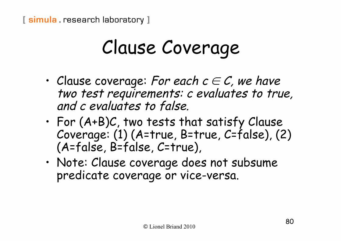
Clause Coverage • Clause coverage: For each c ∈ C, we have
two test requirements: c evaluates to true, and c evaluates to false.
• For (A+B)C, two tests that satisfy Clause Coverage: (1) (A=true, B=true, C=false), (2) (A=false, B=false, C=true),
• Note: Clause coverage does not subsume predicate coverage or vice-versa.
© Lionel Briand 2010 81
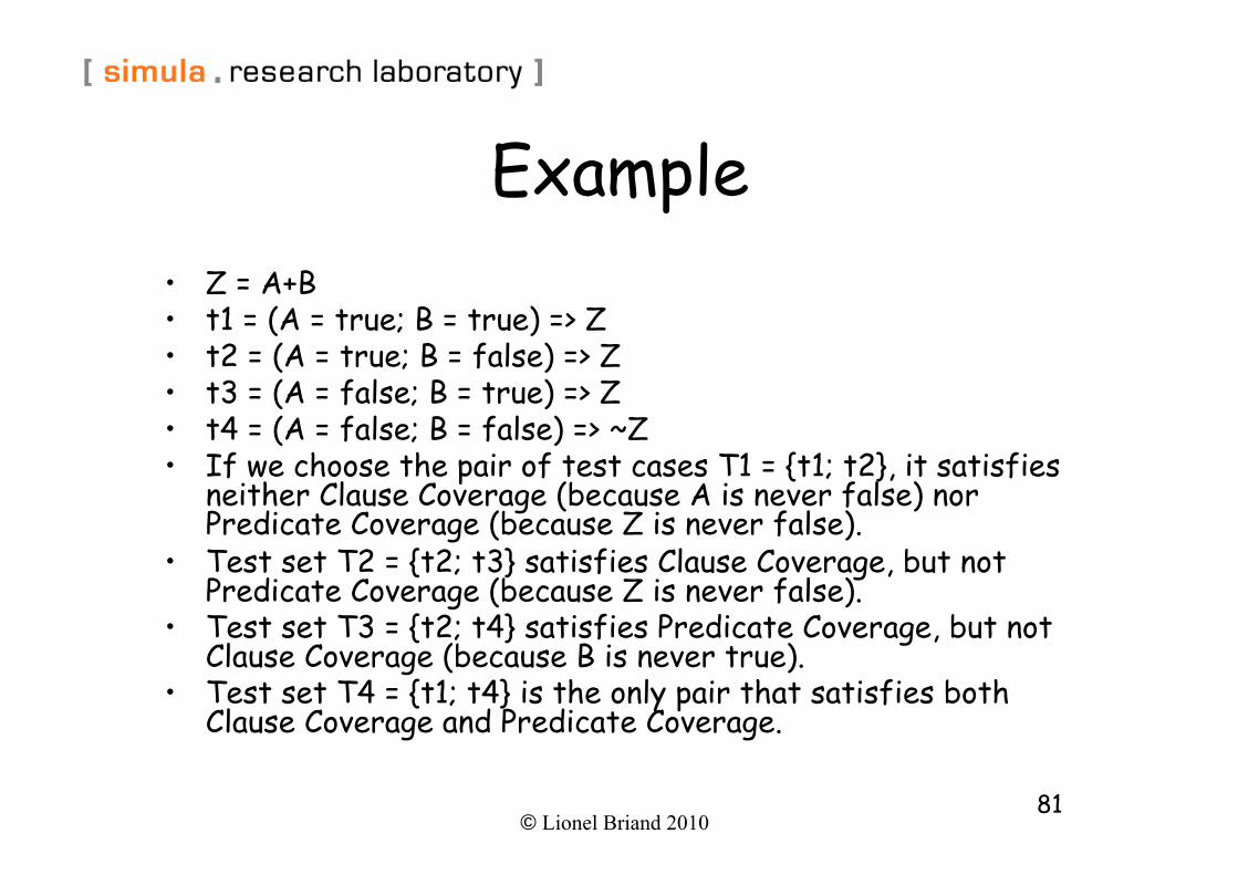
Example • Z = A+B • t1 = (A = true; B = true) => Z • t2 = (A = true; B = false) => Z • t3 = (A = false; B = true) => Z • t4 = (A = false; B = false) => ~Z • If we choose the pair of test cases T1 = {t1; t2}, it satisfies
neither Clause Coverage (because A is never false) nor Predicate Coverage (because Z is never false).
• Test set T2 = {t2; t3} satisfies Clause Coverage, but not Predicate Coverage (because Z is never false).
• Test set T3 = {t2; t4} satisfies Predicate Coverage, but not Clause Coverage (because B is never true).
• Test set T4 = {t1; t4} is the only pair that satisfies both Clause Coverage and Predicate Coverage.
© Lionel Briand 2010 82
Combinatorial Coverage • Combinatorial coverage: For each p∈ P, we
have test requirements for clauses in Cp to evaluate each possible combination of truth values
• Subsumes predicate coverage • There are 2|Cp| possible assignments of
truth values • Problem: Impractical for predicates with
more than a few clauses
© Lionel Briand 2010 83
Masking Effects • When we introduce tests at the clause
level, we want to have an effect on the predicate
• Logical expressions (clauses) can mask each others
• In the predicate AB, if B = false, B can be said to mask A, because no matter what value A has, AB will still be false.
• We need to consider circumstances under which a clause affects the value of a predicate, to detect possible implementation failures
© Lionel Briand 2010 84
Determination • Determination: Given a clause ci in predicate p,
called the major clause, we say that ci determines p if the remaining minor clauses cj∈ p, j <> i have values so that changing the truth value of ci changes the truth value of p.
• We would like to test each clause under circumstances where it determines the predicate
• Test set T4 in previous slide satisfied both predicate and clause coverage but does not test neither A nor B effectively.

© Lionel Briand 2010 85
Active Clause Coverage • Active Clause Coverage (ACC): For each p∈P and each
major clause ci ∈ Cp, choose minor clauses cj, j <> i so that ci determines p. We have two test requirements for each ci: ci evaluates to true and ci evaluates to false.
• For example, for Z=A+B, we end up with a total of four test requirements, two for clause A and two for clause B.
• For clause A, A determines Z if and only if B is false. So we have the two test requirements {(A = true; B =false); (A = false; B = false)}.
• For clause B, B determines Z if and only if A is false. So we have the two test requirements {(A = false; B = true); (A = false; B = false)}, the latter in common with A.
• ACC almost identical to MCDC in code coverage • The most important questions are whether (1) ACC should
subsume PC, (2) the minor clauses cj need to have the same values when the major clause ci is true as when ci is false.
© Lionel Briand 2010 86
Correlated ACC (CACC) • For each p ∈ P and each major clause ci ∈
Cp, choose minor clauses cj, j <> i so that ci determines p. There are two test requirements for each ci: ci evaluates to true and ci evaluates to false. The values chosen for the minor clauses cj must cause p to be true for one value of the major clause ci and false for the other, that is, it is required that p(ci = true) < > p(ci = false).
• CACC is subsumed by combinatorial clause coverage and subsumes clause/predicate coverage
© Lionel Briand 2010 87
Restricted ACC (RACC) • For each p ∈ P and each major clause ci ∈ Cp, choose minor
clauses cj, j <> i so that ci determines p. There are two test requirements for each ci : ci evaluates to true and ci evaluates to false. The values chosen for the minor clauses cj must be the same when ci is true as when ci is false, that is, it is required that cj(ci = true) = cj(ci = false) for all cj .
• RACC makes it easier than CACC to determine the cause of the problem, if one is detected: major clause
• But is it common in specification to have constraints between clauses, making RACC impossible to achieve.
• This corresponds to MCDC for code coverage
© Lionel Briand 2010 88
Example • Z=A(B+C) • It would be possible to satisfy Correlated
Active Clause Coverage with respect to clause A with the two test requirements:
{(A = true; B = true; C = false); (A = false; B =false; C = true)} • But it does not satisfy RACC: {(A = true; B = true; C = false); (A = false; B = true; C = false)} • This case is easy …
© Lionel Briand 2010 89
Inactive Clause Coverage • The Active Clause Coverage Criteria focus on
making sure the major clauses do affect their predicates. A complementary criterion to Active Clause Coverage ensures that changing a major clause that should not affect the predicate does not, in fact, affect the predicate.
• Inactive Clause Coverage (ICC): For each p ∈ P and each major clause ci ∈ Cp, choose minor clauses cj , j <> i so that ci does not determine p. There are four test requirements for ci under these circumstances: (1) ci evaluates to true with p true, (2) ci evaluates to false with p true, (3) ci evaluates to true with p false, and (4) ci evaluates to false with p false.
• ICC is subsumed by combinatorial clause coverage and subsumes clause/predicate coverage
© Lionel Briand 2010 90
Disjunctive Normal Form Coverage Criteria
• Here criteria assume the predicates have been re-expressed in a disjunctive normal form (DNF).
• What is interesting with DNF are the criteria that go with it.
• Criteria: – Implicant coverage – Prime implicant coverage – Variable negation strategy
© Lionel Briand 2010 91
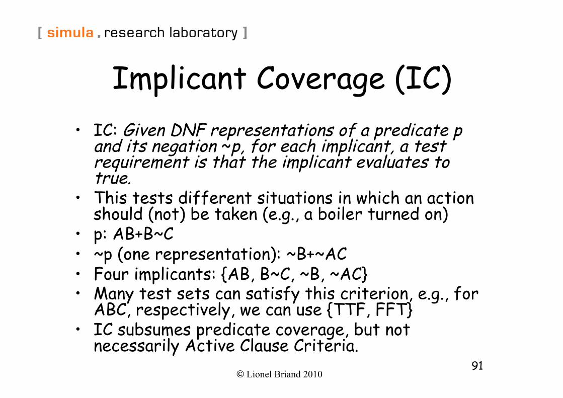
Implicant Coverage (IC) • IC: Given DNF representations of a predicate p
and its negation ~p, for each implicant, a test requirement is that the implicant evaluates to true.
• This tests different situations in which an action should (not) be taken (e.g., a boiler turned on)
• p: AB+B~C • ~p (one representation): ~B+~AC • Four implicants: {AB, B~C, ~B, ~AC} • Many test sets can satisfy this criterion, e.g., for
ABC, respectively, we can use {TTF, FFT} • IC subsumes predicate coverage, but not
necessarily Active Clause Criteria.
© Lionel Briand 2010 92
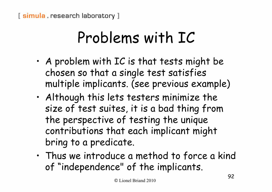
Problems with IC • A problem with IC is that tests might be
chosen so that a single test satisfies multiple implicants. (see previous example)
• Although this lets testers minimize the size of test suites, it is a bad thing from the perspective of testing the unique contributions that each implicant might bring to a predicate.
• Thus we introduce a method to force a kind of “independence" of the implicants.
© Lionel Briand 2010 93
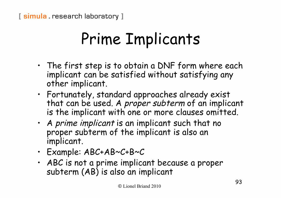
Prime Implicants • The first step is to obtain a DNF form where each
implicant can be satisfied without satisfying any other implicant.
• Fortunately, standard approaches already exist that can be used. A proper subterm of an implicant is the implicant with one or more clauses omitted.
• A prime implicant is an implicant such that no proper subterm of the implicant is also an implicant.
• Example: ABC+AB~C+B~C • ABC is not a prime implicant because a proper
subterm (AB) is also an implicant
© Lionel Briand 2010 94
Prime Implicant Coverage (PIC)
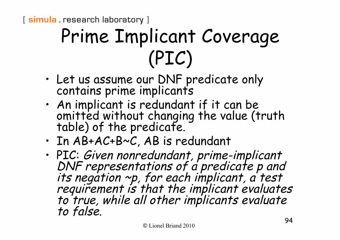
• Let us assume our DNF predicate only contains prime implicants
• An implicant is redundant if it can be omitted without changing the value (truth table) of the predicate.
• In AB+AC+B~C, AB is redundant • PIC: Given nonredundant, prime-implicant
DNF representations of a predicate p and its negation ~p, for each implicant, a test requirement is that the implicant evaluates to true, while all other implicants evaluate to false.
© Lionel Briand 2010 95
PIC Example & Discussion • p: AB+B~C • ~p: ~B+~AC • Both are nonredundant, prime implicant
representations • The following test set satisfies PIC: {TTT, FTF,
FFF, FTT} • PIC is a powerful coverage criteria: none of the
clause coverage criteria subsume PIC • Though up to 2n-1 prime implicants, many
predicates generate a modest number of tests for PIC
• It is an open question whether PIC subsumes any of the clause coverage criteria.
© Lionel Briand 2010 96
Variable Negation Strategy • Goes even further than PIC • Unique true points: variants that makes one and only one
product term true – E.g., (TTFF) for the first product term in the boiler
example (AB~C), AD is false • Near false points: variants for each product term where one
clause is negated such that the overall logic function evaluates to false – E.g., (TTTF) for AB~C where ~C is negated
• Such variants constitute Test Candidate Sets (TCS) • Generate TCS for each product term in logic function • The test suite is formed by selecting the smallest suite that
covers all TCSs
© Lionel Briand 2010 97
Discussion • If one product term implementation does not evaluate to
true when it should - implying that at least one clause in that product term does not evaluate to true when expected - test cases from the TCS (unique true points ) corresponding to the term will be able to detect it, without masking effect from other clauses or terms
• If one product term implementation does not evaluate to false when it should, that is the negation of (at least) a clause has not the effect expected on the logic function (false), test cases from the TCS (near false points ) corresponding to the negated clause will be able to detect it, without masking effect from other clauses or terms
• In a study by Weyuker et al, roughly 6 percent of the All-Variant test suite (2 n) is needed to meet the variable negation criteria
© Lionel Briand 2010 98
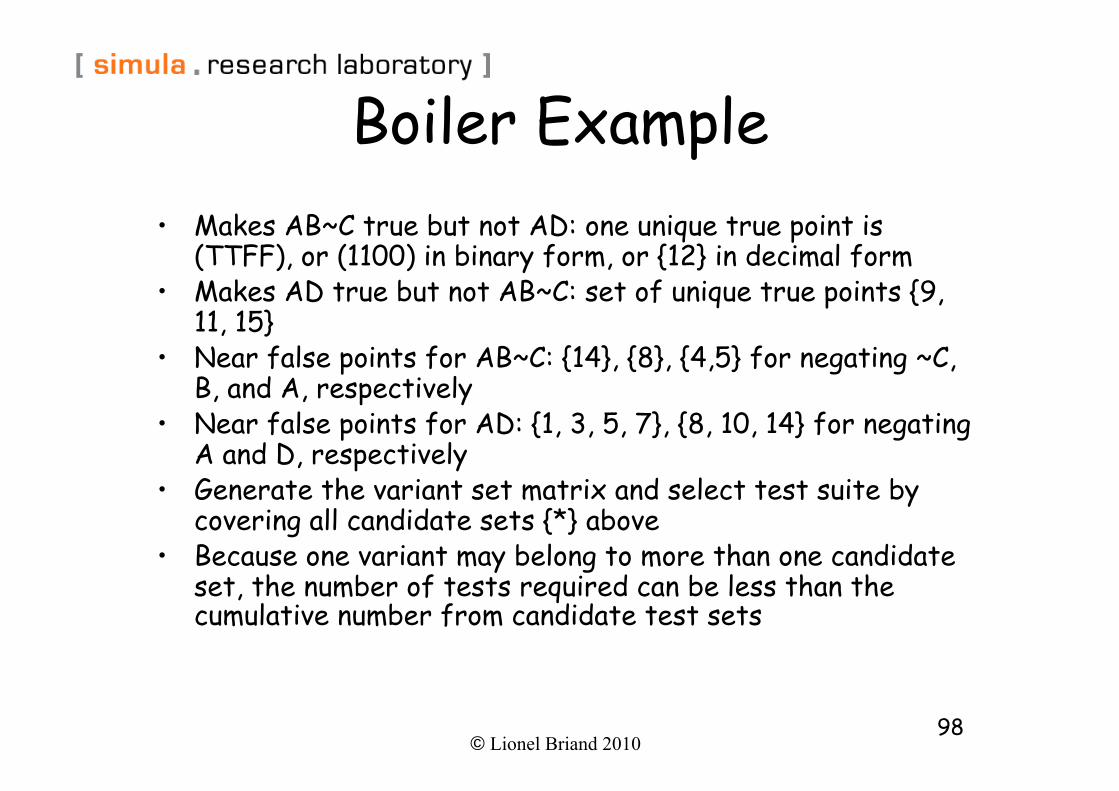
Boiler Example • Makes AB~C true but not AD: one unique true point is
(TTFF), or (1100) in binary form, or {12} in decimal form • Makes AD true but not AB~C: set of unique true points {9,
11, 15} • Near false points for AB~C: {14}, {8}, {4,5} for negating ~C,
B, and A, respectively • Near false points for AD: {1, 3, 5, 7}, {8, 10, 14} for negating
A and D, respectively • Generate the variant set matrix and select test suite by
covering all candidate sets {*} above • Because one variant may belong to more than one candidate
set, the number of tests required can be less than the cumulative number from candidate test sets
© Lionel Briand 2010 99
Variant Set
Matrix
Var 1 2 3 4 5 6 7 TCS 0 1 x 2 3 x 4 x 5 x x S 6 7 x 8 x x S 9 x 10 x 11 x S 12 x S 13 14 x x S 15 x
© Lionel Briand 2010 100
VN Strategy versus Faults • Expression Negation Fault (ENF): Any point in the Boolean
space • Clause Negation Fault (CNF): Any unique true point or near
false point for the faulty term and clause negated • Term Omission Fault (TOF): Any unique true point for the
faulty term • Operator Reference Fault (ORF):
– or implemented as and: Any unique true point of one of the two terms
– and implemented as or: any near false point of one of the two terms
• Clause Omission Fault (COF): Any near false point for the faulty term and clause omitted
• Clause Insertion Fault (CIF): All near false points and unique true points for the faulty term
• Clause Reference Fault (CRF): All near false points and unique true points for the faulty term
© Lionel Briand 2010 101
TCASII Study • TCASII, aircraft collision avoidance system • 20 predicates/logic functions formed the
specifications (in modified statechart notation) • On average 10 distinct clauses per expression • Five mutation operators, defined for boolean
expressions, were used to seed faults in the specifications
• Random selection of test cases (same size) leads to an average mutation score of 42.7%
• The variable negation strategy is therefore doing much better with an average of 97.9%
© Lionel Briand 2010 102
Summary of BB Testing • All techniques see a program as a mathematical
function that maps inputs onto its outputs • By order of sophistication: (1) boundary value
analysis, (2) equivalence class testing, (3) Category-partition (4) Cause-effect graphs
• (1) Mechanical, (2) devise equivalence classes, (3) partitions, categories, and logical dependencies (4) logical dependencies between causes themselves, and causes and effects
• Less test cases with (3) or (4) • Trade-off between test identification and test
execution effort