biz2121-04 production & operations management -...
TRANSCRIPT

BIZ2121-04 Production & Operations Management
Process Quality
Sung Joo Bae, Assistant Professor
Yonsei University School of Business
Disclaimer: Many slides in this presentation file are from the copyrighted material in 2010 by Pearson
Education, Inc. Publishing as Prentice Hall.

Verizon’s effort in quality control
Video: “Can you hear me now?” Campaign
Tear-down analysis & thorough testing on
H/W
Network test (H/W test on the side)
◦ 1M miles/year testing trip
◦ 3M voice calls and 16M data tests
Customer involvement (SKT, KT)

Costs of Quality
A failure to satisfy a customer is considered a defect Defects cause cost
◦ Prevention costs
Preventing defects before they happen
Redesign the processes and products/services
Continuous improvement by employees
Suppliers involvement
◦ Appraisal costs
Costs incurred to identify and assess performance problems

Costs of Quality
◦ Internal failure costs
Costs resulting from defects that are discovered
during the production of service/product
Rework – some aspect of product/service should
be performed again
Scrap – the item is unfit for further processing
◦ External failure costs
Costs that arise when a defect is discovered after
the customer received the service or product

Total Quality Management
Figure 5.1 – TQM Wheel
Customer
satisfaction
A philosophy that stresses three principles for high levels of process
performance and quality

Total Quality Management
Customer satisfaction (internal & external)
◦ Conformance to specifications (e.g.
consistent quality, on-time delivery, delivery
speed)
◦ Value (= Benefit – Cost)
◦ Fitness for use (product features or service
convenience)
◦ Support
◦ Psychological impressions (atmosphere,
image, or aesthetics)

Total Quality Management
Employee involvement ◦ Cultural change – quality at the source
Teams ◦ Problem-solving teams (aka Quality Circles)
Small groups of supervisors and employees who identify, analyze, and solve process/quality problems
◦ Special-purpose teams Focus on an important issue such as new policy
implementation, new technology implementation, etc.
◦ Self-managed teams Highest level of worker participation
Members learn all the tasks involved in the operation
Job rotation
Managerial duties – vacation scheduling, hiring, etc.
Design processes

Total Quality Management
Continuous improvement
◦ Kaizen (改善)
◦ A philosophy of continually seeking ways to improve processes
◦ Not unique to quality – applies to process improvement as well.
Problem-solving tools (such as SPC – statistical process control) should be given
Make SPC a normal aspect of daily operations
Build work teams and employee involvement
Develop operator ownership in the process

The Deming Wheel
Plan
Do
Study
Act
Figure 5.2 – Plan-Do-Study-Act Cycle Problem-solving process

Six Sigma
Figure 5.3 – Six-Sigma Approach Focuses on Reducing Spread and Centering the Process
X X
X X
X X
X
X X
X X X
X X X
X X
Process average OK; too much variation
Process variability OK; process off target
Process on target with low variability Reduce
spread Center process
X
X
X
X
X
X X
X
X
• A comprehensive and flexible system for achieving success by
minimizing defects and variability in the process.
• Driven by understanding customer needs & use of facts, data and
statistical methods

Six Sigma Improvement Model
Continuous efforts in achieving process goals
Assumes the analyzability of the processes
Emphasizes the involvement from the entire organization, especially the senior management
Control
Improve
Analyze
Measure
Define
Figure 5.4 – Six Sigma Improvement Model

Six Sigma Improvement Model

Acceptance Sampling
Application of statistical techniques
Acceptable quality level (AQL) ◦ Criteria for defects that will be accepted (e.g. 5 parts per
100,000)
◦ Sample testing should pass this level. Otherwise the full-scale
inspection should be done.
Linked through supply chains

Acceptance Sampling Firm A uses TQM or Six
Sigma to achieve internal process performance
Supplier uses TQM or Six Sigma to achieve internal
process performance
Yes No
Yes No
Figure 5.5 – Interface of Acceptance Sampling and Process
Performance Approaches in a Supply Chain
Accept blades?
Supplier
Manufactures fan blades
TARGET: Firm A’s specs
Accept motors?
Motor inspection
Blade inspection
Firm A
Manufacturers furnace fan motors
TARGET: Buyer’s specs
Buyer
Manufactures furnaces

Statistical Process Control
Used to detect process change
◦ A increase in the average number of complaints per day at a hotel
◦ An increase in the number of scrapped units at a milling machine
Variation of outputs
◦ Performance measurement Mean Location; Range or S.D. Spread
Variables: continuous scale (length of time, diameter of parts)
Attributes: discrete scale (conformance to complex specification)
◦ Sampling Complete inspection
When cost of failure matters
Automated inspection
Sampling When inspection cost is high and inspection affects the product or service
Sample size
Interval between successive samples
Decision rules on when to take actions

Sampling Distributions
1. The sample mean is the sum of the observations divided by the total number of observations
n
x
x
n
i
i 1
where
xi = observation of a quality characteristic (such as time)
n = total number of observations
x = mean

Sampling Distributions
The range is the difference between the largest observation
in a sample and the smallest.
The standard deviation is the square root of the variance of
a distribution. An estimate of the process standard
deviation based on a sample is given by
where
σ = standard deviation of a sample
1 or
1
2
2
n
n
xx
n
xxi
ii
2

Sample and Process Distributions
Distribution of sample means
25 Time
Mean
Process distribution
Figure 5.6 – Relationship Between the Distribution of Sample
Means and the Process Distribution

Causes of Variation in Process Distribution
Common causes
◦ Random, unavoidable sources of variation
◦ Characterized by
Location - mean
Spread – s.d. or range
Shape – symmetrical or skewed
Assignable causes
Can be identified and eliminated
Change in the mean, spread, or shape
Used after a process is in statistical control
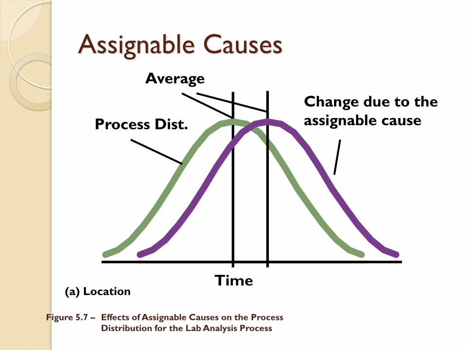
Assignable Causes
(a) Location Time
Average
Figure 5.7 – Effects of Assignable Causes on the Process
Distribution for the Lab Analysis Process
Process Dist.
Change due to the
assignable cause

Assignable Causes
(b) Spread Time
Average
Figure 5.7 – Effects of Assignable Causes on the Process
Distribution for the Lab Analysis Process

Assignable Causes
(c) Shape Time
Average
Figure 5.7 – Effects of Assignable Causes on the Process
Distribution for the Lab Analysis Process

Control Charts
Time-ordered diagram of process performance
◦ Mean
◦ Upper control limit
◦ Lower control limit
Steps for a control chart
1. Random sample
2. Plot statistics
3. Eliminate the cause, incorporate improvements
4. Repeat the procedure

Control Charts
Samples
Assignable causes likely
1 2 3
Figure 5.8 – How Control Limits Relate to the Sampling Distribution:
Observations from Three Samples
UCL
Nominal
LCL

Nominal
UCL
LCL
Vari
ati
on
s
Sample number
Control Charts
Figure 5.9 – Control Chart Examples
(a) Normal – No action

Nominal
UCL
LCL
Vari
ati
on
s
Sample number
Control Charts
Figure 5.9 – Control Chart Examples
(b) Run – Take action
Run usually involves five or more observations show a trend (upward/downward)

Nominal
UCL
LCL
Vari
ati
on
s
Sample number
Control Charts
Figure 5.9 – Control Chart Examples
(c) Sudden change – Monitor

Nominal
UCL
LCL
Vari
ati
on
s
Sample number
Control Charts
Figure 5.9 – Control Chart Examples
(d) Exceeds control limits – Take action
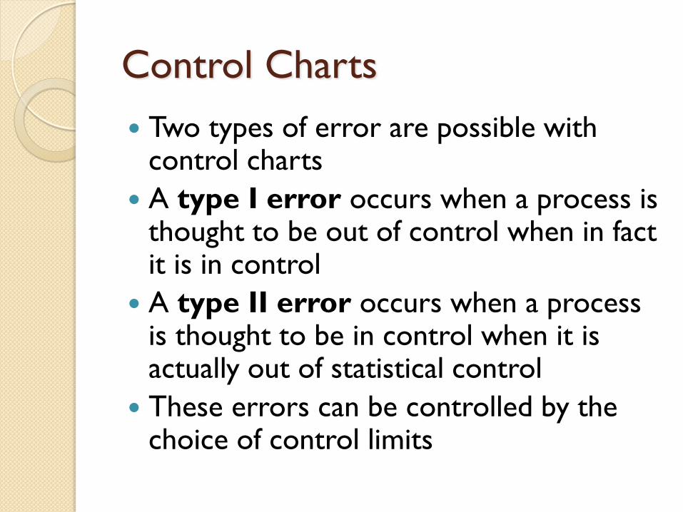
Control Charts
Two types of error are possible with control charts
A type I error occurs when a process is thought to be out of control when in fact it is in control
A type II error occurs when a process is thought to be in control when it is actually out of statistical control
These errors can be controlled by the choice of control limits

Control Charts – Error control by
the choice of the control limits
Wider limits Larger type II error cost for not detecting a shift
Smaller type I error < search cost for assignable causes
Narrower limits Larger type I error search cost for assignable causes
Smaller type II error < cost for not detecting a shift
Time
Average
A type I error occurs when a process is thought to be out of control when in fact it is in control
A type II error occurs when a process is thought to be in control when it is actually out of statistical control

SPC Methods Used for monitoring current process performance & for detecting any changes in the process
Control charts for variables
◦ R-Chart, or range chart
◦ For monitoring the process variability
UCLR = D4R and LCLR = D3R
where
R = average of several past R (range) values and the central line of the control chart
D3, D4 = constants that provide three standard deviation (three-sigma) limits for the given sample size

Control Chart Factors
TABLE 5.1 | FACTORS FOR CALCULATING THREE-SIGMA LIMITS FOR | THE x-CHART AND R-CHART
Size of Sample (n)
Factor for UCL and LCL for x-Chart (A2)
Factor for LCL for R-Chart (D3)
Factor for UCL for R-Chart (D4)
2 1.880 0 3.267
3 1.023 0 2.575
4 0.729 0 2.282
5 0.577 0 2.115
6 0.483 0 2.004
7 0.419 0.076 1.924
8 0.373 0.136 1.864
9 0.337 0.184 1.816
10 0.308 0.223 1.777

SPC Methods
UCLx = x + A2R and LCLx = x – A2R
Control charts for variables
x-Chart
where
x = central line of the chart, which can be either the average of past sample means or a target value set for the process
A2 = constant to provide three-sigma limits for the sample mean

Steps for x- and R-Charts
1. Collect data
2. Compute the range
3. Use Table 5.1 to determine R-chart control limits
4. Plot the sample ranges. If all are in control, proceed to step 5. Otherwise, find the assignable causes, correct them, and return to step 1.
5. Calculate x for each sample

Steps for x- and R-Charts
6. Use Table 5.1 to determine x-chart control limits
7. Plot the sample means. If all are in control, the process is in statistical control. Continue to take samples and monitor the process.
If any are out of control, find the assignable causes, correct them, and return to step 1. If no assignable causes are found, assume out-of-control points represent common causes of variation and continue to monitor the process.

Using x- and R-Charts EXAMPLE 5.1
The management of West Allis Industries is concerned about the
production of a special metal screw used by several of the company’s
largest customers. The diameter of the screw is critical to the customers.
Data from five samples appear in the accompanying table. The sample size
is 4. Is the process in statistical control?
SOLUTION
Step 1: For simplicity, we use only 5 samples. In practice, more than 20 samples would be desirable. The data are shown in the following table.
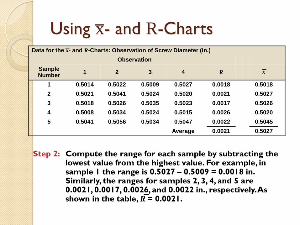
Using x- and R-Charts Data for the x- and R-Charts: Observation of Screw Diameter (in.)
Observation
Sample Number
1 2 3 4 R x
1 0.5014 0.5022 0.5009 0.5027 0.0018 0.5018
2 0.5021 0.5041 0.5024 0.5020 0.0021 0.5027
3 0.5018 0.5026 0.5035 0.5023 0.0017 0.5026
4 0.5008 0.5034 0.5024 0.5015 0.0026 0.5020
5 0.5041 0.5056 0.5034 0.5047 0.0022 0.5045
Average 0.0021 0.5027
Step 2: Compute the range for each sample by subtracting the lowest value from the highest value. For example, in sample 1 the range is 0.5027 – 0.5009 = 0.0018 in. Similarly, the ranges for samples 2, 3, 4, and 5 are 0.0021, 0.0017, 0.0026, and 0.0022 in., respectively. As shown in the table, R = 0.0021.

Using x- and R-Charts Step 3: To construct the R-chart, select the appropriate
constants from Table 5.1 for a sample size of 4. The control limits are
UCLR = D4R = 2.282(0.0021) = 0.00479 in.
0(0.0021) = 0 in. LCLR = D3R =
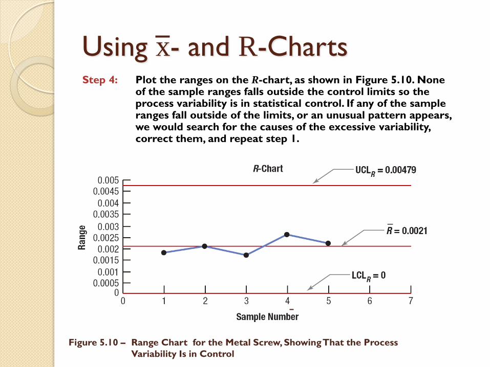
Using x- and R-Charts
Figure 5.10 – Range Chart for the Metal Screw, Showing That the Process
Variability Is in Control
Step 4: Plot the ranges on the R-chart, as shown in Figure 5.10. None of the sample ranges falls outside the control limits so the process variability is in statistical control. If any of the sample ranges fall outside of the limits, or an unusual pattern appears, we would search for the causes of the excessive variability, correct them, and repeat step 1.

Using x- and R-Charts
Step 5: Compute the mean for each sample. For example, the mean for sample 1 is
0.5014 + 0.5022 + 0.5009 + 0.5027
4 = 0.5018 in.
Similarly, the means of samples 2, 3, 4, and 5 are 0.5027, 0.5026, 0.5020, and 0.5045 in., respectively. As shown in the table, x = 0.5027.

Using x- and R-Charts Data for the x- and R-Charts: Observation of Screw Diameter (in.)
Observation
Sample Number
1 2 3 4 R x
1 0.5014 0.5022 0.5009 0.5027 0.0018 0.5018
2 0.5021 0.5041 0.5024 0.5020 0.0021 0.5027
3 0.5018 0.5026 0.5035 0.5023 0.0017 0.5026
4 0.5008 0.5034 0.5024 0.5015 0.0026 0.5020
5 0.5041 0.5056 0.5034 0.5047 0.0022 0.5045
Average 0.0021 0.5027

Using x- and R-Charts
LCLx = x – A2R =
0.5027 + 0.729(0.0021) = 0.5042 in.
0.5027 – 0.729(0.0021) = 0.5012 in.
UCLx = x + A2R
Step 6: Now construct the x-chart for the process average. The average screw diameter is 0.5027 in., and the average range is 0.0021 in., so use x = 0.5027, R = 0.0021, and A2 from Table 5.1 for a sample size of 4 to construct the control limits:
Using x- and R-Charts
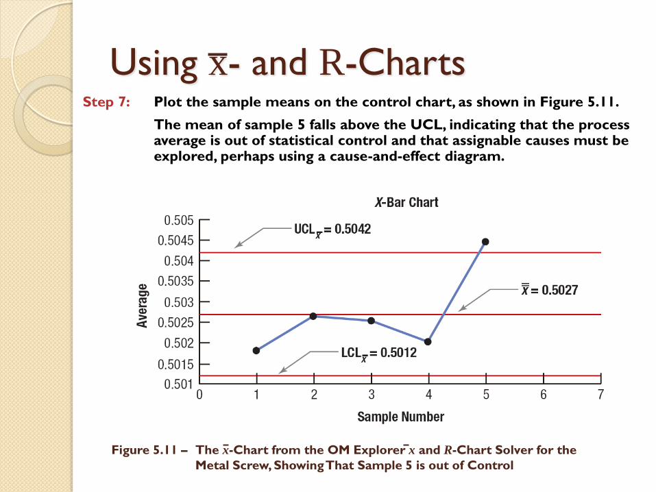
Figure 5.11 – The x-Chart from the OM Explorer x and R-Chart Solver for the
Metal Screw, Showing That Sample 5 is out of Control
Step 7: Plot the sample means on the control chart, as shown in Figure 5.11.
The mean of sample 5 falls above the UCL, indicating that the process average is out of statistical control and that assignable causes must be explored, perhaps using a cause-and-effect diagram.

Application 5.1 Webster Chemical Company produces mastics and caulking for the
construction industry. The product is blended in large mixers and then
pumped into tubes and capped.
Webster is concerned whether the filling process for tubes of caulking
is in statistical control. The process should be centered on 8 ounces per
tube. Several samples of eight tubes are taken and each tube is weighed
in ounces.
Tube Number
Sample 1 2 3 4 5 6 7 8 Avg Range
1 7.98 8.34 8.02 7.94 8.44 7.68 7.81 8.11 8.040 0.76
2 8.23 8.12 7.98 8.41 8.31 8.18 7.99 8.06 8.160 0.43
3 7.89 7.77 7.91 8.04 8.00 7.89 7.93 8.09 7.940 0.32
4 8.24 8.18 7.83 8.05 7.90 8.16 7.97 8.07 8.050 0.41
5 7.87 8.13 7.92 7.99 8.10 7.81 8.14 7.88 7.980 0.33
6 8.13 8.14 8.11 8.13 8.14 8.12 8.13 8.14 8.130 0.03
Avgs 8.050 0.38
Q: Assuming that taking only 6 samples is sufficient, is the process in statistical control?

Application 5.1 Webster Chemical Company produces mastics and caulking for the
construction industry. The product is blended in large mixers and then
pumped into tubes and capped.
Webster is concerned whether the filling process for tubes of caulking is in
statistical control. The process should be centered on 8 ounces per tube.
Several samples of eight tubes are taken and each tube is weighed in
ounces.
Tube Number
Sample 1 2 3 4 5 6 7 8 Avg Range
1 7.98 8.34 8.02 7.94 8.44 7.68 7.81 8.11 8.040 0.76
2 8.23 8.12 7.98 8.41 8.31 8.18 7.99 8.06 8.160 0.43
3 7.89 7.77 7.91 8.04 8.00 7.89 7.93 8.09 7.940 0.32
4 8.24 8.18 7.83 8.05 7.90 8.16 7.97 8.07 8.050 0.41
5 7.87 8.13 7.92 7.99 8.10 7.81 8.14 7.88 7.980 0.33
6 8.13 8.14 8.11 8.13 8.14 8.12 8.13 8.14 8.130 0.03
Avgs 8.050 0.38
Q: Assuming that taking only 6 samples is sufficient, is the process in statistical control?

Application 5.1 Assuming that taking only 6 samples is sufficient, is the process in statistical control?
UCLR = D4R =
LCLR = D3R =
1.864(0.38) = 0.708
0.136(0.38) = 0.052
The range chart is out of control since sample 1 falls outside the
UCL and sample 6 falls outside the LCL. This means that the x
calculation is not necessary.
Conclusion on process variability given R = 0.38 and n = 8:
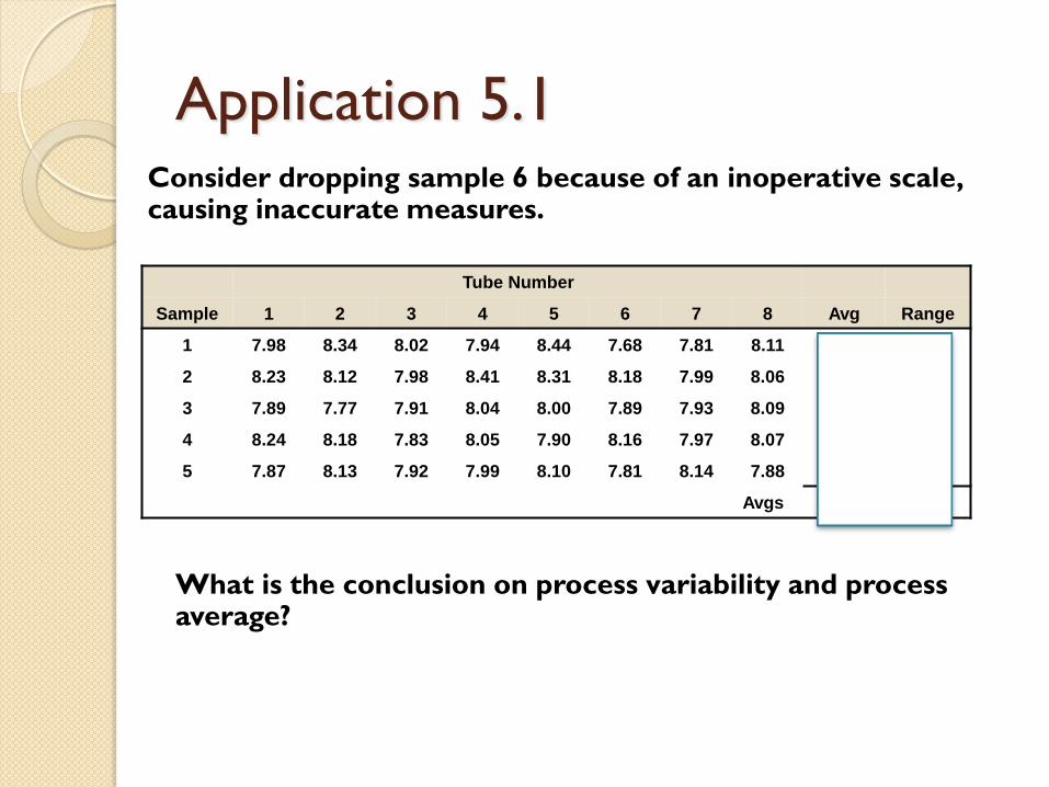
Application 5.1 Consider dropping sample 6 because of an inoperative scale, causing inaccurate measures.
Tube Number
Sample 1 2 3 4 5 6 7 8 Avg Range
1 7.98 8.34 8.02 7.94 8.44 7.68 7.81 8.11 8.040 0.76
2 8.23 8.12 7.98 8.41 8.31 8.18 7.99 8.06 8.160 0.43
3 7.89 7.77 7.91 8.04 8.00 7.89 7.93 8.09 7.940 0.32
4 8.24 8.18 7.83 8.05 7.90 8.16 7.97 8.07 8.050 0.41
5 7.87 8.13 7.92 7.99 8.10 7.81 8.14 7.88 7.980 0.33
Avgs 8.034 0.45
What is the conclusion on process variability and process average?
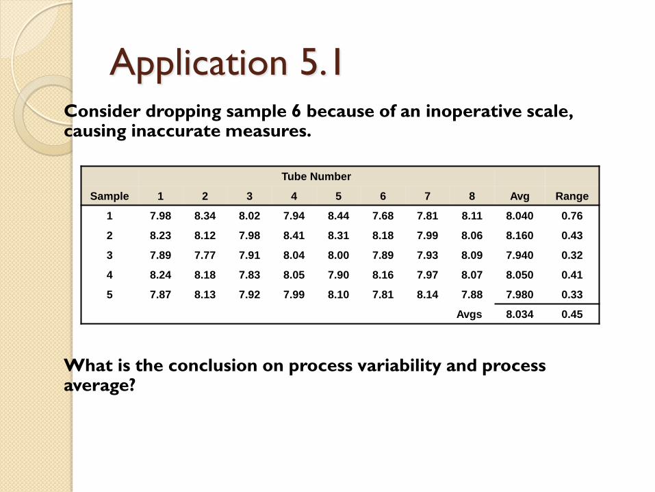

Application 5.1
UCLR = D4R =
LCLR = D3R =
1.864(0.45) = 0.839
0.136(0.45) = 0.061
UCLx = x + A2R =
LCLx = x – A2R =
8.034 + 0.373(0.45) = 8.202
8.034 – 0.373(0.45) = 7.832
Now R = 0.45, x = 8.034, and n = 8
The resulting control charts indicate that the process is actually in control.

Process Capability
Process capability refers to the ability of the process to meet the design specification for the product or service
Design specifications are often expressed as a nominal value (target) and a tolerance (allowance)

Process Capability
20 25 30 Minutes
Upper
specification
Lower
specification
Nominal
value
(a) Process is capable
Process distribution
Figure 5.14 – The Relationship Between a Process Distribution and
Upper and Lower Specifications
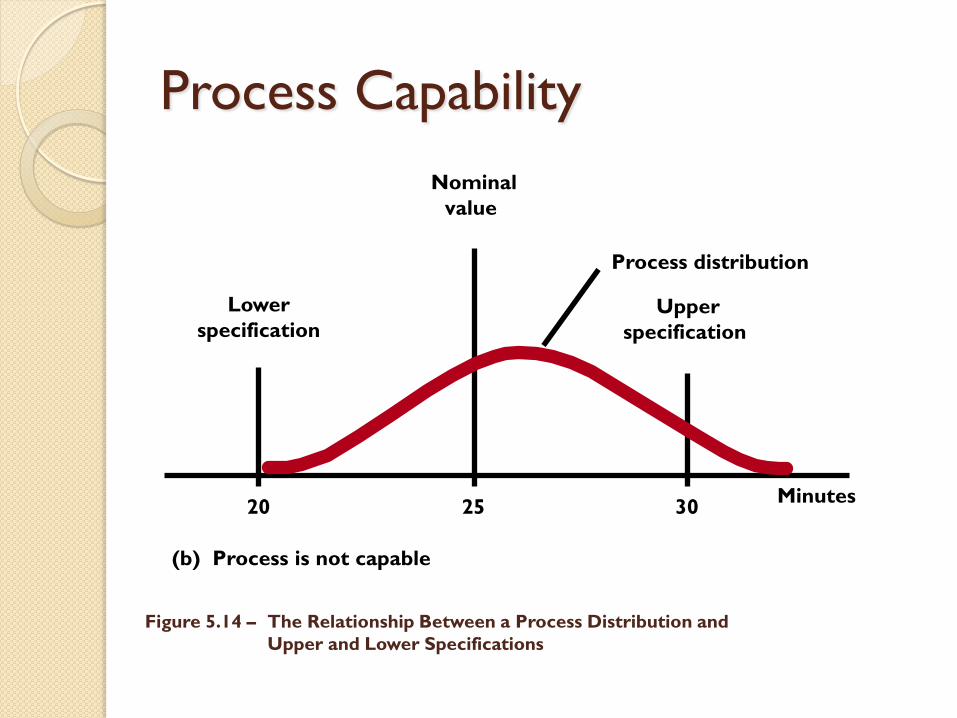
Process Capability
20 25 30 Minutes
Upper
specification
Lower
specification
Nominal
value
(b) Process is not capable
Figure 5.14 – The Relationship Between a Process Distribution and
Upper and Lower Specifications
Process distribution

Process Capability
Figure 5.15 – Effects of Reducing Variability on Process Capability
Lower
specification
Mean
Upper
specification
Nominal value
Six sigma
Four sigma
Two sigma

Process Capability
The process capability index measures how well a process is centered and whether the variability is acceptable
Cpk = Minimum of , x – Lower specification
3σ
Upper specification – x
3σ
where
σ = standard deviation of the process distribution

Process Capability
The process capability ratio tests whether
process variability is the cause of problems
Cp = Upper specification – Lower specification
6σ

Determining Process Capability
Step 1. Collect data on the process output, and calculate the mean and the standard deviation of the process output distribution.
Step 2. Use the data from the process distribution to compute process control charts, such as an x- and an R-chart.

Determining Process Capability
Step 3. Take a series of at least 20 consecutive random
samples from the process and plot the results on the
control charts. If the sample statistics are within the
control limits of the charts, the process is in
statistical control. If the process is not in statistical
control, look for assignable causes and eliminate
them. Recalculate the mean and standard deviation
of the process distribution and the control limits for
the charts. Continue until the process is in statistical
control.

Determining Process Capability
Step 4. Calculate the process capability index. If the results are
acceptable, the process is capable and document any
changes made to the process; continue to monitor the
output by using the control charts. If the results are
unacceptable, calculate the process capability ratio. If
the results are acceptable, the process variability is fine
and management should focus on centering the
process. If not, management should focus on reducing
the variability in the process until it passes the test. As
changes are made, recalculate the mean and standard
deviation of the process distribution and the control
limits for the charts and return to step 3(control
chart).

Assessing Process Capability
EXAMPLE 5.5
The intensive care unit lab process has an average turnaround time of 26.2 minutes and a standard deviation of 1.35 minutes
The nominal value for this service is 25 minutes with an upper specification limit of 30 minutes and a lower specification limit of 20 minutes
The administrator of the lab wants to have four-sigma performance for her lab
Is the lab process capable of this level of performance?

Assessing Process Capability SOLUTION
The administrator began by taking a quick check to see if the process is
capable by applying the process capability index:
Lower specification calculation = = 1.53 26.2 – 20.0
3(1.35)
Upper specification calculation = = 0.94 30.0 – 26.2
3(1.35)
Cpk = Minimum of [1.53, 0.94] = 0.94
Since the target value for four-sigma performance is 1.33, the process capability index told her that the process was not capable. However, she did not know whether the problem was the variability of the process, the centering of the process, or both. The options available to improve the process depended on what is wrong.

Assessing Process Capability
She next checked the process variability with the process capability ratio:
The process variability did not meet the four-sigma target of 1.33. Consequently, she initiated a study to see where variability was introduced into the process. Two activities, report preparation and specimen slide preparation, were identified as having inconsistent procedures. These procedures were modified to provide consistent performance. New data were collected and the average turnaround was now 26.1 minutes with a standard deviation of 1.20 minutes.
Cp = = 1.23 30.0 – 20.0
6(1.35)
Assessing Process Capability
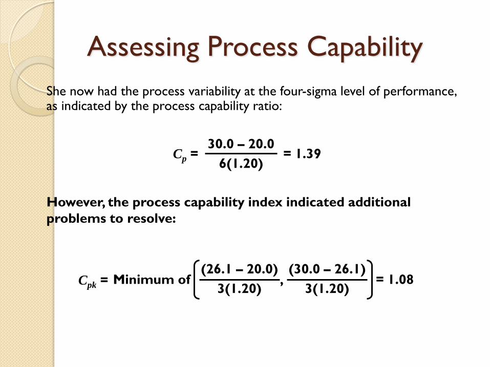
She now had the process variability at the four-sigma level of performance, as indicated by the process capability ratio:
However, the process capability index indicated additional
problems to resolve:
Cp = = 1.39 30.0 – 20.0
6(1.20)
Cpk = , = 1.08 (26.1 – 20.0)
3(1.20)
(30.0 – 26.1)
3(1.20) Minimum of

Application 5.4 Webster Chemical’s nominal weight for filling tubes of caulk is 8.00 ounces ± 0.60 ounces. The target process capability ratio is 1.33, signifying that management wants 4-sigma performance. The current distribution of the filling process is centered on 8.054 ounces with a standard deviation of 0.192 ounces. Compute the process capability index and process capability ratio to assess whether the filling process is capable and set properly.

Application 5.4
Recall that a capability index value of 1.0 implies that the firm is producing three-sigma quality (0.26% defects) and that the process is consistently producing outputs within specifications even though some defects are generated. The value of 0.948 is far below the target of 1.33. Therefore, we can conclude that the process is not capable. Furthermore, we do not know if the problem is centering or variability.
Cpk = Minimum of , x – Lower specification
3σ
Upper specification – x
3σ
= Minimum of = 1.135, = 0.948 8.054 – 7.400
3(0.192)
8.600 – 8.054
3(0.192)
a. Process capability index:

Application 5.4
b. Process capability ratio:
Cp = Upper specification – Lower specification
6σ = = 1.0417
8.60 – 7.40
6(0.192)
Recall that if the Cpk is greater than the critical value (1.33 for
four-sigma quality) we can conclude that the process is capable.
Since the Cpk is less than the critical value, either the process
average is close to one of the tolerance limits and is generating
defective output, or the process variability is too large. The value
of Cp is less than the target for four-sigma quality. Therefore we
conclude that the process variability must be addressed first, and
then the process should be retested.

Quality Engineering
Quality engineering is an approach originated by Genichi Taguchi that involves combining engineering and statistical methods to reduce costs and improve quality by optimizing product design and manufacturing processes.
The quality loss function is based on the concept that a service or product that barely conforms to the specifications is more like a defective service or product than a perfect one.

Quality Engineering
Lo
ss (
do
llars
)
Lower Nominal Upper
specification value specification
Figure 5.16 – Taguchi’s Quality Loss Function

International Standards
ISO 9000:2000 addresses quality management
by specifying what the firm does to fulfill the
customer’s quality requirements and applicable
regulatory requirements while enhancing
customer satisfaction and achieving continual
improvement of its performance
Companies must be certified by an external
examiner
Assures customers that the organization is
performing as they say they are

International Standards
ISO 14000:2004 documents a firm’s environmental program by specifying what the firm does to minimize harmful effects on the environment caused by its activities
The standards require companies to keep track of their raw materials use and their generation, treatment, and disposal of hazardous wastes
Companies are inspected by outside, private auditors on a regular basis

International Standards
External benefits are primarily increased
sales opportunities
ISO certification is preferred or required by
many corporate buyers
Internal benefits include improved
profitability, improved marketing, reduced
costs, and improved documentation and
improvement of processes
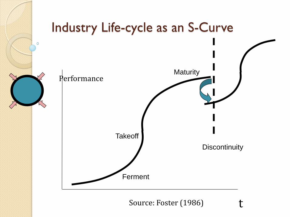
Industry Life-cycle as an S-Curve
t
Performance
Source: Foster (1986)
Discontinuity
Ferment
Takeoff
Maturity
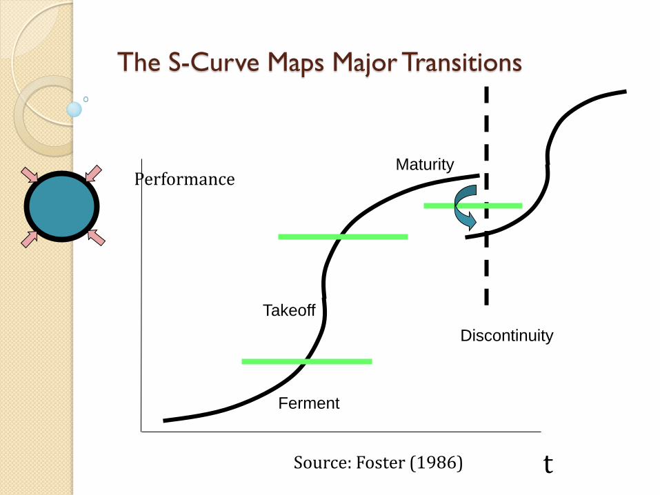
The S-Curve Maps Major Transitions
t
Performance
Source: Foster (1986)
Discontinuity
Ferment
Takeoff
Maturity

Success trap
Fit
Congruence in strategy, critical tasks, people, org
design, culture
Success
Size & Age
Organizations get larger, more structured, & older
Inertia
Success
in stable environment
or
Failure
When environments shifts
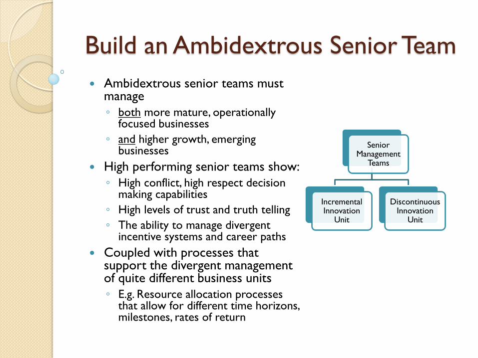
Build an Ambidextrous Senior Team
Ambidextrous senior teams must manage
◦ both more mature, operationally focused businesses
◦ and higher growth, emerging businesses
High performing senior teams show:
◦ High conflict, high respect decision making capabilities
◦ High levels of trust and truth telling
◦ The ability to manage divergent incentive systems and career paths
Coupled with processes that support the divergent management of quite different business units
◦ E.g. Resource allocation processes that allow for different time horizons, milestones, rates of return
Senior Management
Teams
Incremental Innovation
Unit
Discontinuous Innovation
Unit
End of Process Quality Session