bivariate extreme statistics, ii - statistics … · for a given pair of joint and marginal...

REVSTAT – Statistical Journal

Volume 10, Number 1, March 2012, 83–107

BIVARIATE EXTREME STATISTICS, II

Authors: Miguel de Carvalho

– Swiss Federal Institute of Technology,Ecole Polytechnique Federale de Lausanne, [email protected]

Centro de Matematica e Aplicacoes, Faculdade de Ciencias e Tecnologia,Universidade Nova de Lisboa, Portugal

Alexandra Ramos

– Universidade do Porto, Faculdade de Economia, [email protected]

Abstract:

• We review the current state of statistical modeling of asymptotically independentdata. Our discussion includes necessary and sufficient conditions for asymptotic inde-pendence, results on the asymptotic independence of statistics of interest, estimationand inference issues, joint tail modeling, and conditional approaches. For each ofthese topics we give an account of existing approaches and relevant methods for dataanalysis and applications.

Key-Words:

• asymptotic independence; coefficient of tail dependence; conditional tail modeling;extremal dependence; hidden regular variation; joint tail modeling; order statistics;maximum; multivariate extremes; sums.

AMS Subject Classification:

• 60G70, 62E20.

84 M. de Carvalho and A. Ramos

Bivariate Extreme Statistics, II 85

1. INTRODUCTION

The concept of asymptotic independence connects two central notions in

probability and statistics: asymptotics and independence. Suppose that X and Y

are identically distributed real-valued random variables, and that our interest is

in assessing the probability of a joint tail event (X > u, Y > u), where u denotes

a high threshold. We say that (X, Y ) is asymptotically independent, Xa. ind.

∼ Y , if

(1.1) limu→∞

pr(X > u | Y > u

)= lim

u→∞

pr(X > u, Y > u

)

pr(Y > u

) = 0 .

Intuitively, condition (1.1) implies that given that the decay of the joint distribu-

tion is faster than the marginals, it is unlikely that the largest values of X and Y

happen simultaneously.1 Whereas independence is unrealistic for many data ap-

plications, there has been a recent understanding that when modeling extremes,

asymptotic independence is often found in real data. It may seem surprising that

although the problem of testing asymptotic independence is an old goal in statis-

tics (Gumbel & Goldstein, 1964), only recently there has been an understanding

that classical models for multivariate extremes are unable to deal with it.

In this paper we review the current state of statistical modeling of asymp-

totically independent data. Our discussion includes a list of important topics,

including necessary and sufficient conditions, results on the asymptotic indepen-

dence of statistics of interest, estimation and inference issues, and joint tail mod-

eling. We also provide our personal view on some directions we think could be

of interest to be explored in the coming years. Our discussion is not exhaustive,

and in particular there are many results of probabilistic interest, on asymptotic

independence of other statistics not relevant to extreme value analyses, which are

not discussed here.

The title of this paper is based on the seminal work of Sibuya (1960), enti-

tled “Bivariate Extreme Statistics, I”which presents necessary and sufficient con-

ditions for the asymptotic independence of the two largest extremes in a bivariate

distribution. Sibuya mentions that a practical application should be “considered

in a subsequent paper” which to our knowledge never appeared.

Other recent surveys on asymptotic independence include Resnick (2002)

and Beirlant et al. (2004, §9). The former mostly explores connections with

hidden regular variation and multivariate second order regular variation.

1To be precise, the tentative definition in (1.1) corresponds simply to a particular instanceof the concept, i.e., asymptotic independence of the largest extremes in a bivariate distribution.Although this is the version of the concept to which we devote most of our attention, the conceptof asymptotic independence is actually broader, and has also been studied for many other pairs ofstatistics, other than bivariate extremes, even in the field of extremes; we revisit some examplesin §6.


2. ASYMPTOTIC INDEPENDENCE—CHARACTERIZATIONS

2.1. Necessary and sufficient conditions for asymptotic independence

Early developments on asymptotic independence of the two largest extremes

in a bivariate distribution, were mostly devoted to obtaining necessary or suffi-

cient characterizations for asymptotic independence (Finkelstein, 1953; Geffroy,

1958, 1959; Sibuya, 1960; Berman, 1961; Ikeda, 1963; Mikhailov, 1974; Galambos,

1975; de Haan & Resnick, 1977; Marshall & Olkin, 1983; Takahashi, 1994).

Geffroy (1958) showed that the condition

(2.1) limx,y→∞

C{FX(x), FY (y)

}

1 − FX,Y (x, y)= 0

is sufficient for asymptotic independence, where the operator

C{FX(x), FY (y)

}≡ pr

(X > x, Y > y

)

= 1 + FX,Y (x, y) − FX(x) − FY (y) , (x, y) ∈ R2 ,

(2.2)

maps a pair of marginal distribution functions to their joint tails. We prefer to

state results using a copula, i.e., a function C : [0, 1]2 → [0, 1], such that

C(p, q) = FX,Y

{F−1

X (p), F−1Y (q)

}, (p, q) ∈ [0, 1]2 .

Here F−1· (·) = inf

{x : F·(x) ≥ · ∈ [0, 1]

}, and the uniqueness of the function C

for a given pair of joint and marginal distributions follows by Sklar’s theorem

(Sklar, 1959). Geffroy’s condition can then be rewritten as

(2.3) limp,q ↑1

C(p, q)

1 − C(p, q)= lim

p,q ↑1

1 + C(p, q) − p − q

1 − C(p, q)= 0 .

Example 2.1. Examples of dependence structures obeying condition (2.3)

can be found in Johnson & Kotz (1972, §41), and include any member of the

Farlie–Gumbel–Morgenstern family of copulas

Cα(p, q) = p q{1 + α(1− p) (1− q)

}, α ∈ [−1, 1] ,

and the copulas of the bivariate exponential and bivariate logistic distributions

(Gumbel, 1960, 1961), respectively given by

Cθ(p, q) = p + q − 1 + (1− p) (1− q) exp{−θ log(1− p) log(1− q)

}, θ ∈ [0, 1] ,

C(p, q) =p q

p + q − p q, (p, q) ∈ [0, 1]2 .


Sibuya (1960) introduced a condition related to (2.1)

(2.4) limq ↑1

C(q, q)

1 − q= 0 ,

and showed that this is necessary and sufficient for asymptotic independence.

Condition (2.4) is simply a reformulation of (1.1) which describes the rate at

which we start lacking observations in the joint tails, as we move towards higher

quantiles. Sibuya used condition (2.4) to observe that bivariate normal dis-

tributed vectors with correlation ρ < 1 are asymptotically independent, and sim-

ilar results are also inherited by light-tailed elliptical densities (Hult & Lindskog,

2002).

Often the question arises on whether it is too restrictive to study asymptotic

independence only for the bivariate case. This question was answered long ago by

Berman (1961), who showed that a d-dimensional random vector Z = (Z1, ..., Zd),

with a regularly varying joint tail (Bingham et al., 1987), is asymptotically inde-

pendent if, and only if,

Zia. ind.

∼ Zj , i 6= j .

Asymptotic independence in a d-vector is thus equivalent to pairwise asymptotic

independence.2 This can also be shown to be equivalent to having the exponent

measure put null mass on the interior of the first quadrant, and to concentrate on

the positive coordinate axes, or equivalently to having all the mass of the spec-

tral measure concentrated on 0 and 1; definitions of the spectral and exponent

measures are given in Beirlant et al. (2004, §8), and a formal statement of this

result can be found in Resnick (1987, Propositions 5.24–25). In theory, this allows

us to restrict the analysis to the bivariate case, so we confine the exposition to

this setting. Using the result of Berman (1961) we can also state a simple neces-

sary and sufficient condition, analogous to (2.4), for asymptotic independence of

Z = (Z1, ..., Zd), i.e.,

limq ↑1

d∑

i=1

d∑

j=1(j 6=i)

Cij(q, q)

1 − q= 0 , Cij(p, q) ≡ 1 + Cij(p, q)− p− q , (p, q) ∈ [0, 1]2 ,

with the obvious notations (Mikhailov, 1974, Theorem 2).

Example 2.2. Consider the copula of bivariate logistic distribution in

Example 2.1. Sibuya’s condition (2.4) follows directly:

limq ↑1

C(q, q)

1 − q= lim

q ↑1

2(q − 1)2

2 − q= 0 .

2The pairwise structure is however insufficient to determine the higher order structure;e.g., in general not much can be inferred on pr

�X > x, Y > y, Z > z

�, from the pairs.


The characterizations in (1.1) and (2.1) are population-based, but a lim-

iting sample-based representation can also be given, using the random sample

{(Xi, Yi)}ni=1, so that asymptotic independence is equivalent to

(2.5) limn→∞

Cn(p1/n, q1/n

)= p q , (p, q) ∈ [0, 1]2 .

In words: the copula of the distribution function of the sample maximum Mn =

max{(X1, Y1), ..., (Xn, Yn)

}, where the maximum are taken componentwise, con-

verges to the product copula Cπ = p q; equivalently we can say that the extreme-

value copula, limn→∞ Cn(p1/n, q1/n

), is Cπ, or that C is in the domain of attrac-

tion of Cπ.

Srivastava (1967) and Mardia (1964) studied results on asymptotic inde-

pendence on bivariate samples, but for other order statistics, rather than the

maximum. Consider a random sample {(Xi, Yi)}ni=1 and the order statistics

X1:n ≤ ··· ≤ Xn:n and Y1:n ≤ ··· ≤ Yn:n. It can be shown that if (X1:n, Y1:n) is

asymptotically independent, then

Xi:na. ind.

∼ Yj:n , i, j ∈ {1, ..., n} .

See Srivastava (1967, Theorem 3).

The last characterization of asymptotic independence we discuss is due to

Takahashi (1994). According to Takahashi’s criterion, asymptotic independence

is equivalent to

(2.6) ∃ (a,b)∈ (0,∞)2 : ℓ(a, b) ≡ limq ↑1

1− C{1− a(1− q), 1− b(1− q)

}

1− q= a+b .

Example 2.3. A simple analytical example to verify Takahashi’s criterion

is given by taking the bivariate logistic copula and checking that ℓ(1, 1) = 2.

Remark 2.1. The function ℓ(a, b) is the so-called stable tail dependence

function, and as shown in Beirlant et al. (2004, p. 286), condition (2.6) is equiv-

alent to

ℓ(a, b) = a + b , (a, b) ∈ [0,∞) .

2.2. Notes and comments

Some of the results obtained in Finkelstein (1953) were ‘rediscovered’ in

later papers. Some of these include results proved by Galambos (1975), who

claims that Finkelstein (1953) advanced his results without giving formal proofs.


Tiago de Oliveira (1962/63) is also acknowledged for pioneering work in sta-

tistical modeling of asymptotic independence of bivariate extremes. Mikhailov

(1974) and Galambos (1975) obtained a necessary and sufficient condition for

d-dimensional asymptotic independence of arbitrary extremes; a related charac-

terization can also be found in Marshall & Olkin (1983, Proposition 5.2)

Most of the characterizations discussed above are directly based on distribu-

tion functions and copulas, but it seems natural to infer asymptotic independence

from contours of the joint density. Balkema & Nolde (2010) establish sufficient

conditions for asymptotic independence, for some homothetic densities, i.e., den-

sities whose level sets all have the same shape. In particular, they show that the

components of continuously differentiable homothetic light-tailed distributions

with convex levels sets are asymptotically independent; in their Corollary 2.1

Balkema and Nolde also show that asymptotic independence resists quite notable

distortions in the joint distribution.

Measures of asymptotic dependence for further order statistics are studied

in Ferreira & Ferreira (2012).

2.3. Dual measures of extremal dependence: (χ, χ)

Many measures of dependence, such as the Pearson correlation coefficient,

Spearman rank correlation, and Kendall’s tau, can be written as functions of

copulae (Schweizer & Wolff, 1981, p. 879), and as we discuss below, measures of

extremal dependence can also be conceptualized as functions of copulae.

To measure extremal dependence we first need to convert the data (X ,Y)

to a common scale. The rescaled variables (X, Y ) are transformed to have unit

Frechet margins, i.e., FX(z) = FY (z) = exp(−1/z), z > 0; this can be done with

the mapping

(2.7) (X ,Y) 7→ (X, Y ) = −({

log FX (X )}−1

,{log FY(Y)

}−1)

.

Since the rescaled variables have the same marginal distribution, any remaining

differences between distributions can only be due to dependence features (Em-

brechts et al., 2002). A natural measure to assess the degree of dependence at an

arbitrary high level τ < ∞, is the bivariate tail dependence index

(2.8) χ = limu→∞

pr(X > u | Y > u

)= lim

q ↑1pr

{X >F−1

X (q) | Y >F−1Y (q)

}.

This measure takes values in [0, 1], and can be used to assess the degree of de-

pendence that remains in the limit (Coles et al., 1999; Poon et al., 2003, 2004).


If dependence persists as u → ∞, then 0 < χ ≤ 1 and X and Y are said to be

asymptotically dependent; otherwise, the degree of dependence vanishes in the

limit, so that χ = 0 and the variables are asymptotically independent. The mea-

sure χ can also be rewritten in terms of the limit of a function of the copula C,

by noticing that

(2.9) χ = limq ↑1

χ(q) , χ(q) = 2 −log C(q, q)

log q, 0 < q < 1 .

Thus, the function C ‘couples’ the joint distribution function and its correspond-

ing marginals, and it also provides helpful information for modeling joint tail

dependence. The function χ(q) can be understood as a quantile dependent mea-

sure of dependence, and the sign of χ(q) can be used to ascertain if the variables

are positively or negatively associated at the quantile q. As a consequence of

the Frechet–Hoeffding bounds (Nelsen, 2006, §2.5), the level of dependence is

bounded,

(2.10) 2 −log(2 q − 1)+

log q≤ χ(q) ≤ 1 , 0 < q < 1 ,

where a+ = max(a, 0), a ∈ R. Extremal dependence should be measured accord-

ing to the dependence structure underlying the variables under analysis. If the

variables are asymptotically dependent, the measure χ is appropriate for as-

sessing the strength of dependence which links the variables at the extremes.

If however the variables are asymptotically independent then χ = 0, so that

χ pools cases where although dependence may not prevail in the limit, it may per-

sist for relatively large levels of the variables. To measure extremal dependence

under asymptotic independence, Coles et al. (1999) introduced the measure

(2.11) χ = limu→∞

2 log pr(X > u

)

log pr(X > u, Y > u

) − 1 ,

which takes values on the interval (−1, 1]. The interpretation of χ is to a certain

extent analogous to that of the Pearson correlation: values of χ > 0, χ = 0

and χ < 0, respectively correspond to positive association, exact independence

and negative association in the extremes, and if the dependence structure is

Gaussian then χ = ρ (Sibuya, 1960). This benchmark case is particularly helpful

for guiding how does the dependence in the tails, as measured by χ, compares

with that arising from fitting a Gaussian dependence model.

Asymptotic dependence and asymptotic independence can also be charac-

terized through χ. For asymptotically dependent variables, it holds that χ = 1,

while for asymptotically independent variables χ takes values in (−1, 1). Hence

χ and χ can be seen as dual measures of joint tail dependence: if χ = 1 and

0 < χ ≤ 1, the variables are asymptotically dependent, and χ assesses the de-

gree of dependence within the class of asymptotically dependent distributions;

if −1 < χ < 1 and χ = 0, the variables are asymptotically independent, and


χ assesses the degree of dependence within the class of asymptotically indepen-

dent distributions. In a similar way to (2.9), the extremal measure χ can also be

written using copulas, viz.

(2.12) χ = limq ↑1

χ(q) , χ(q) =2 log(1 − q)

log C(q, q).

Hence, the function C can provide helpful information for assessing dependence

in extremes both under asymptotic dependence and asymptotic independence.

The function χ(q) has an analogous role to χ(q), in the case of asymptotic inde-

pendence, and it can also be used as quantile dependent measure of dependence,

with the following Frechet–Hoeffding bounds:

(2.13)2 log(1 − q)

log(1 − 2 q)+− 1 ≤ χ(q) ≤ 1 , 0 < q < 1 .

For an inventory of the functional forms of the extremal measures χ and χ,

over several dependence models, see Heffernan (2000). We remark that the dual

measures (χ, χ) can be reparametrized as

(2.14) (χ, χ) = (2− θ, 2 η −1) ,

where θ = limq ↑1 log C(q, q)/ log q is the so-called extremal coefficient, and η is

the coefficient of tail dependence to be discussed in §3–4.

3. ESTIMATION AND INFERENCE

3.1. Coefficient of tail dependence-based approaches

The coefficient of tail dependence η corresponds to the extreme value index

of the variable Z = min{X, Y }, which characterizes the joint tail behavior above a

high threshold u (Ledford & Tawn, 1996). The formal details are described in §4,

but the heuristic argument follows by the simple observation that

pr(Z > u) = pr

(X > u, Y > u

),

and hence we reduce a bivariate problem to a univariate one. This implies that we

can use the order statistics of the Zi = min{Xi, Yi}, Z(1)≤ ··· ≤Z(n), to estimate η

by applying univariate estimation methods, such as the Hill estimator

ηk =1

k

k∑

i=1

{log Z(n−k+i) − log Z(n−k)

}.

By estimating η directly with univariate methods we are however underestimating

its uncertainty, since we ignore the uncertainty from transforming the data to

equal margins, say by using (2.7). The estimators of Peng (1999), Draisma et al.

(2004), Beirlant & Vandewalle (2002), can be used to tackle this, and a review of

these methods can be found in Beirlant et al. (2004, pp. 351–353).


3.2. Score-based tests

Tawn (1988) and Ledford & Tawn (1996) proposed score statistics for exam-

ining independence within the class of multivariate extreme value distributions.

Ramos & Ledford (2005) proposed modified versions of such tests which solve the

problem of slow rate of convergence of such tests, due to infinite variance of the

scores. Consider the following partition of the outcome space R2+, given by

Rkl ={

(x, y) : k = I(x > u), l = I(y > u)}

, k, l ∈ {0, 1} ,

where u denotes a high threshold and I denotes the indicator function. The

approach of Ramos and Ledford is based on censoring the upper tail R11 for a high

threshold u, so that, using the logistic dependence structure, the score functions

at independence of Tawn (1988) and Ledford & Tawn (1996) are respectively

given by

U1n =

∑

(Xi,Yi) /∈R11

∆1(Xi, Yi) + Λ , U2n =

∑

(Xi,Yi) /∈R11

∆2(Xi, Yi) + Λ ,

where

∆1(Xi, Yi) = (1−X−1i ) logXi + (1−Y −1

i ) logYi

+ (2 −X−1i −Y −1

i ) log(X−1i +Y −1

i ) − (X−1i +Y −1

i )−1 ,

∆2(Xi, Yi) = I{(Xi, Yi) ∈ Rkl

}Skl(Xi, Yi) ,

Λ =2 u−1 log 2 exp(−2 u−1)N

2 exp(−u−1) − exp(−2 u−1) − 1,

with N denoting the number of observations in region R11, and

S00(x, y) = −2 u−1 log 2 ,

S01(x, y) = −u−1 log u + (1− y−1) log y + (1− u−1− y−1) log(u−1 + y−1) ,

S10(x, y) = −u−1 log u + (1− x−1) log x + (1− x−1− u−1) log(x−1 + u−1) ,

S11(x, y) = (1− x−1) log x + (1− y−1) log y + (2− x−1− y−1) log(x−1 + y−1)

− (x−1 + y−1)−1 .

The modified score functions U1n and U2

n have zero expectation and finite second

moments. The limit distributions under independence are then given as

−n−1/2 U in

σi

d−→ N(0, 1) , n → ∞ , i = 1, 2 ,

whered

−→ denotes convergence in distribution and σi denotes the variance of the

corresponding modified score statistics; we remark that these score tests typically

reject independence when evaluated on asymptotically independent data.


3.3. Falk–Michel test

Falk & Michel (2006) proposed tests for asymptotic independence based on

the characterization

(3.1)

(Xa. ind.

∼ Y ) ≡

{Fδ(t) = pr

(X−1+Y −1 < δ t

∣∣ X−1+Y −1 < δ)−→δ→0

t2 , t∈ [0,1]

}.

Alternatively, under asymptotic dependence we have pointwise convergence of

Fδ(t) → t, for t ∈ [0, 1], as δ → 0. Falk & Michel (2006) use condition (3.1) to

test for asymptotic independence of (X, Y ) using a battery of classical goodness-

of-fit tests. An extension of their method can be found in Frick et al. (2007).

3.4. Gamma test

Zhang (2008) introduced the tail quotient correlation to assess extremal

dependence between random variables. If u is a positive high threshold, and W

and V are exceedance values over u of X and Y , then the tail quotient correlation

coefficient is defined as

(3.2) qu,n =max

{(u + Wi)/(u + Vi)

}n

i=1+ max

{(u + Vi)/(u + Wi)

}n

i=1− 2

max{(u + Wi)/(u + Vi)

}n

i=1max

{(u + Vi)/(u + Wi)

}n

i=1− 1

.

Asymptotically, qu,n can take values between zero and one. If both max{(u+Wi)/

(u +Vi)}n

i=1and max

{(u + Vi)/(u + Wi)

}n

i=1are large, so that large values of

both variables tend to occur one at a time, qu,n will be close to zero. If the two

‘max’ are close to one, then qu,n approaches one, and hence large values of both

variables tend to occur together. There is a connection to the tail dependence

index χ in (2.8): if χ is zero, then qu,n converges to zero almost surely. So if

(X, Y ) is asymptotically independent, qu,n is close to zero, although, in practice,

the tail quotient correlation coefficient may never reach zero. This brings us to

the hypotheses

H0 : (X, Y ) is asymptotically independent ,

H1 : (X, Y ) is asymptotically dependent .

The Gamma test for asymptotic independence says that as n → ∞,

n qu,nd

−→ Γ{2, 1− exp(−1/u)

}.

A large value of qu,n is indicative of tail dependence and thus leads to a smaller

p-value. If H0 is rejected, we can use qu,n as measure of extremal dependence.


Although it might seem that the tail quotient correlation increases as u increases,

this is not the case as an increase in u leads to a decrease in the scale parameter

1 − exp(−1/u), leading to a larger α-percentile.

The tail quotient correlation in (3.2) is an extension of another measure of

dependence—the quotient correlation—which is defined as

(3.3) qn =max{Yi/Xi}

ni=1 + max{Xi/Yi}

ni=1 − 2

max{Yi/Xi}ni=1 × max{Xi/Yi}n

i=1 − 1.

Zhang et al. (2011) shows that (3.3) is asymptotically independent of the Pearson

correlation ρn, meaning that qn and ρn measure different degrees of association

between random variables, in a large sample setting.

3.5. Madogram test

Bacro et al. (2010) propose to test for asymptotic independence using a

madogram

W =1

2

∣∣FX(X) − FY (Y )∣∣ ,

which is a tool often used in geostatistics to capture spatial structures. The ex-

pected value and the variance of the madogram depend on the extremal coefficient

as follows:

µW =1

2

(θ − 1

θ + 1

), σ2

W =1

6− µ2

W −1

2

∫ 1

0

dt{1 + A(t)

}2 ,

where A is the Pickands’ dependence function, which is related to the spectral

measure H, as follows:

A(t) = 2

∫ 1

0max

{w(1− t), (1−w)t

}dH(w) .

Hence testing for asymptotic independence (θ = 2) is the same as testing if

µW = 1/6. Inference is made on the basis of the asymptotic result

n1/2

(µW − 1/6

σW

)d

−→ N(0, 1)

where µW and σW are consistent estimators of µ and σ.


Other tests of independence between marginal extremes include a Cramer–

von Mises-type statistic by Deheuvels & Martynov (1996), a dependence function


based test by Deheuvels (1980), a test based on the number of points below certain

thresholds by Dorea & Miasaki (1993), the dependence function approaches of

Caperaa et al. (1997). The behavior of Kendall’s-τ as a measure of dependence

within extremes has been also examined; see Caperaa et al. (2000) and Genest

& Rivest (2001). An alternative likelihood-based approach that uses additional

occurrence time information is given in Stephenson & Tawn (2005), and Ramos &

Ledford (2009) propose likelihood ratio-based tests for asymptotic independence,

asymmetry, and ray independence, resulting from a joint tail modeling approach

which we describe in §4.2.

The huge literature on inference for asymptotic independence itself requires

an entire survey. The criterion for selecting the methods presented above was

mainly their simplicity, but many other methods exist which would also meet

this criterion; see de Haan & de Ronde (1998), Husler & Li (2009), Tsai et al.

(2011), among others.

4. JOINT TAIL MODELS

4.1. Joint tail specifications

We start by discussing three different regular variation-based specifications

that provide the basis for the joint tail models to be discussed. The idea is

to provide a chronological view on the different specifications considered on ex-

tremal dependence models that accommodate both asymptotic dependence and

asymptotic independence. Most of the emphasis is placed on the Ramos–Ledford

spectral model.

Let (X ,Y) be a bivariate random variable with joint distribution function

FX ,Y with margins FX and FY ; we apply (2.7) to obtain a pair of unit Frechet

distributed random variables, X and Y . Ledford & Tawn (1996) proposed the

following specification for the joint survival function:

FX,Y (x, x) = pr(X > x, Y > x

)=

ℓ(x)

x1/η,

where η ∈ (0, 1] is the coefficient of tail dependence and ℓ is a slowly varying

function, i.e., limx→∞ ℓ(tx)/ℓ(x) = 1, for all t > 0.

Ledford & Tawn (1997, 1998) proposed the more flexible joint asymptotic

expansion

(4.1) FX,Y (x, y) = pr(X > x, Y > x) =

L(x, y)

xc1 yc2, c1 + c2 = η ,


where L is a bivariate slowly varying function, i.e., there is a function g, the

so-called limit function of L, such that for all x, y > 0 and c > 0

(4.2) g(x, y) ≡ limr→∞

{L(rx, ry)

L(r, r)

}, g(cx, cy) = g(x, y) .

The so-called ray dependence function is then defined as

g∗(w) ≡ g(x, y) , w = x/(x + y) ∈ [0, 1] .

If g∗(w) varies with w, we say that L(x,y) is ray dependent; if otherwise g∗(w) =1,

w ∈ (0, 1), we say that is ray independent.

Ramos & Ledford (2009) considered a particular case of specification (4.1)

where c1= c2, i.e.,

(4.3) FX,Y (x, y) = pr(X > x, Y > x

)=

L(x, y)

(xy)1/(2η).

4.2. Ramos–Ledford spectral model

Ramos & Ledford (2009) base their analysis on the bivariate conditional

random variable (S, T ) = limu→∞

{(X/u, Y/u) : (X > u, Y > u)

}, for a high thresh-

old u. The joint survivor function of the conditional random variable (S, T ) is

such that

FST (s, t) = pr(S > s, T > t

)

= limu→∞

pr(X > su, Y > tu

)

pr(X > u, Y > u

)

= η

∫ 1

0

{min

(w

s,1−w

t

)}1/η

dHη(w) ,

(4.4)

where Hη is a non-negative measure on [0, 1] that should obey the normalization

constraint

(4.5)

∫ 1/2

0w1/η dHη(w) +

∫ 1

1/2(1 − w)1/η dHη(w) =

1

η.

The measure Hη is analogous to the spectral measure H in classical models for

multivariate extremes, which in turn must obey normalization and marginal mo-

ment constraints:∫ 1

0dH(w) = 1 ,

∫ 1

0w dH(w) =

1

2.

The two measures can be related: for example, if η = 1, dH1(w) = χ×2 dH(w)

(Ramos & Ledford, 2009, p. 240), with χ = 2 −∫ 10 max(w, 1−w) dH(w). The


measure Hη is a particular case of the hidden angular measure, which has been

studied by Resnick (2002) and Maulik & Resnick (2004), but in these papers the

normalization constraint (4.5) has been omitted.

Using the joint tail specification (4.3) we can also relate the joint survivor

function of the conditional random variable (S, T ) with the ray dependence func-

tion g⋆, as follows:

FST (s, t) = limu→∞

{L(us, ut)

L(u, u)(st)1/(2η)

}=

g(s, t)

(st)1/(2η)=

g∗{s/(s + t)

}

(st)1/(2η).

Treating the limit in (4.4) as an approximation in the joint tail, we have that for

a sufficiently large threshold u

(4.6) FX,Y (x, y) ≈ FX,Y (u, u)FS,T (x/u, y/u) , (x, y) ∈ (u,∞)2 .

For an arbitrary (X ,Y) with joint distribution function FX ,Y , with margins FX

and FY , we apply (2.7) to obtain a pair of unit Frechet distributed random

variables, X and Y . The joint survivor function of (X ,Y) can then be modelled

by

F(X ,Y)(x, y) = λ FST

{−1

u log FX (x),

−1

u log FY(y)

}, (x, y) ∈ (u1,∞)×(u2,∞) ,

where λ denotes the probability of falling in R11. Ramos & Ledford (2009) also

showed that for this approach to yield a complete joint tail characterization, the

marginal tails of the survivor function of S and T must satisfy certain monotonic-

ity conditions, implying that their marginal tails cannot be heavier than the unit

Frechet survivor function. These conditions guarantee that a given function FST

can arise as a limit in equation (4.4).

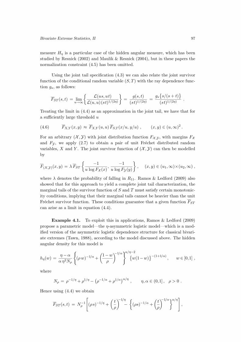
Example 4.1. To exploit this in applications, Ramos & Ledford (2009)

propose a parametric model—the η-asymmetric logistic model—which is a mod-

ified version of the asymmetric logistic dependence structure for classical bivari-

ate extremes (Tawn, 1988), according to the model discussed above. The hidden

angular density for this model is

hη(w) =η −α

α η2Nρ

{(ρ w)−1/α +

(1−w

ρ

)−1/α}α/η−2{

w(1−w)}−(1+1/α)

, w ∈ [0,1] ,

where

Nρ = ρ−1/η + ρ1/η −(ρ−1/α + ρ1/α

)α/η, η, α ∈ (0,1] , ρ > 0 .

Hence using (4.4) we obtain

FST (s, t) = N−1ρ

[(ρs)−1/η +

(t

ρ

)−1/η

−

{(ρs)−1/α +

(t

ρ

)−1/α}α/η]

,


so that by (4.6) the joint survival model for (X, Y ) is

FX,Y (x, y) = FX,Y (u, u)×u1/η

Nρ

[(ρx)−1/η +

(y

ρ

)−1/η

−

{(ρx)−1/α +

(y

ρ

)−1/α}α/η]

,

for (x, y) ∈ [u,∞)2.

4.3. Curse of dimensionality?

The model admits a d-dimensional generalization, where the hidden angular

measure now needs to obey the normalization constraint

(4.7)

∫

∆d

min{w1, ..., wd}1/η dHη(w) = 1/η ,

where ∆d = {w ∈Rd+ :

∑di=1 wi = 1; w = (w1, ..., wd)

}. The corresponding con-

straints that the angular measure needs to obey are

(4.8)

∫

∆d

w dH(w) = 1 ,

∫

∆d

w dH(w) = d−11d ,

Hence, whereas in classical models for multivariate extremes d +1 constraints

need to be fulfilled, in the d-dimensional version of the Ramos–Ledford model

only one constraint needs to be fulfilled.

A d-dimensional version of the η-asymmetric model discussed in Exam-

ple 4.1 can be found in Ramos & Ledford (2011, p. 2221).


Qin et al. (2008) discuss a device for obtaining further parametric speci-

fications for the Ramos–Ledford model, using a construction similar to Coles &

Tawn (1991). Whereas Coles & Tawn (1991) propose a method that transforms

any positive measure on the simplex to satisfy the constraints (4.8), Qin et al.

(2008) propose a method that transforms any positive measure on the simplex, to

satisfy the Ramos–Ledford constraint (4.7). Qin et al. (2008) use their device to

produce a Dirichlet model for the hidden angular density hη. Ramos & Ledford

(2011) give a point process representation that supplements the model discussed

above.

Wadsworth & Tawn (2012a) propose a model based on a specification on

which the axis along which the extrapolation is performed is ‘tilted’ by assum-

ing that the marginals grow at different rates. They also obtain analogues of


the Pickands and exponent functions for this setting, and propose the so-called

inverted multivariate extreme value distributions, which are models for asymp-

totic independence, having a one-to-one correspondence with multivariate ex-

treme value distributions; any construction principle or model generator for a

multivariate extreme value distributed X can thus be readily adapted to create

a inverted multivariate extreme value distributed Y . The link between multi-

variate extreme value distributions and their inverted versions allows the use

of approaches which are amenable to non/semi-parametric methods for a mod-

erate number of dimensions, and it also convenient for parametric modeling of

high-dimensional extremes; for example, the max-mixture max{aX, (1− a)Y },

a ∈ [0, 1], can then be used as a hybrid model, and this principle is adapted for

spatial modeling of extremes in Wadsworth & Tawn (2012b).

Maxima of moving maxima (M4) processes have been recently extended by

Heffernan et al. (2007) to produce models for asymptotic independence.

5. CONDITIONAL TAIL MODELS

5.1. Conditional tail specification

The models discussed in §4 focused on the joint tails, but under asymptotic

independence it may be restrictive to confine the analysis to such region. Heffer-

nan & Tawn (2004) propose conditional tail models, where the focus is on events

where at least one component of (X, Y ) is extreme, where here we now assume

Gumbel marginal distributions. We thus need to model the distribution of X |Y

when Y is large, and of Y |X when X is large; for concreteness we focus on

the latter. Analogously to the joint tail modeling, a limiting specification is also

needed here: we assume that there exist norming functions a(u) and b(u) > 0,

such that

(5.1) limu→∞

pr

{Y − b(u)

a(u)≤ e | X = u

}= G(e) .

To ensure that Y has no mass at ∞, G needs to satisfy

limz→∞

G(z) = 1 .

We define the auxiliary variable ε = {Y − b(u)}/a(u), so that specification (5.1)

can be rewritten as limu→∞ pr(ε≤ e |X = u

)= G(e).


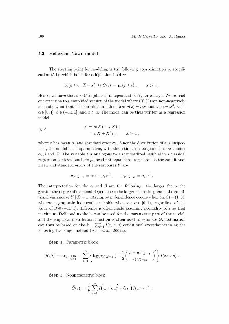
5.2. Heffernan–Tawn model

The starting point for modeling is the following approximation to specifi-

cation (5.1), which holds for a high threshold u:

pr(ε ≤ ǫ | X = x

)≈ G(ǫ) = pr

(ε ≤ ǫ

), x > u .

Hence, we have that ε ∼ G is (almost) independent of X, for u large. We restrict

our attention to a simplified version of the model where (X, Y ) are non-negatively

dependent, so that the norming functions are a(x) = αx and b(x) = xβ , with

α∈ [0, 1], β ∈ (−∞, 1], and x > u. The model can be thus written as a regression

model

Y = a(X) + b(X)ε

= αX + Xβε , X > u ,(5.2)

where ε has mean µε and standard error σε. Since the distribution of ε is unspec-

ified, the model is semiparametric, with the estimation targets of interest being

α, β and G. The variable ε is analogous to a standardized residual in a classical

regression context, but here µε need not equal zero in general, so the conditional

mean and standard errors of the responses Y are

µY |X=x = αx + µεxβ , σY |X=x = σεxβ .

The interpretation for the α and β are the following: the larger the α the

greater the degree of extremal dependence; the larger the β the greater the condi-

tional variance of Y |X = x. Asymptotic dependence occurs when (α, β) = (1, 0),

whereas asymptotic independence holds whenever α ∈ [0, 1), regardless of the

value of β ∈ (−∞, 1). Inference is often made assuming normality of ε so that

maximum likelihood methods can be used for the parametric part of the model,

and the empirical distribution function is often used to estimate G. Estimation

can thus be based on the k =∑n

i=1 I(xi > u) conditional exceedances using the

following two-stage method (Keef et al., 2009a):

Step 1. Parametric block

(α, β) = arg max(α,β)

−n∑

i=1

{log(σY |X=xi

) +1

2

(yi − µY |X=xi

σY |X=xi

)2}

I(xi > u) .

Step 2. Nonparametric block

G(e) =1

k

n∑

i=1

I(yi ≤ e x

bβi + αxi

)I(xi > u) .


As an alternative to Step 2 we can also obtain a kernel estimate as follows:

(5.3) G(e) =1

k

n∑

i=1

K

(e −

yi − αxi

xbβ )I(xi > u) ,

with K denoting a kernel and h > 0 its bandwidth. This procedure suffers how-

ever from a weakness common to all two-stage approaches: uncertainty is under-

estimated in the second step.


Heffernan & Resnick (2007) provide a mathematical examination of a mod-

ified Heffernan–Tawn model and its connections with hidden regular variation.

A version of the model able to cope with missing data can be found in Keef

et al. (2009b). For applications see, for instance, Paulo et al. (2006), Keef et al.

(2009a), and Hilal et al. (2011).

6. REMARKS ON THE ONE-SAMPLE FRAMEWORK

6.1. Asymptotic independence of order statistics

The expression “asymptotic independence”did not appear for the first time

in the works of Geffroy (1958, 1959) and Sibuya (1960), in the context of statistics

of extremes. The concept was motivated by a conjecture that Gumbel made

on the joint limiting distribution of pairs of order statistics, in a one-sample

framework:

“In a previous article [1] the assumption was used that the mth obser-vation in ascending order (from the bottom) and the mth observation indescending order (from the top) are independent variates, provided thatthe rank m is small compared to the sample size n.” (Gumbel, 1946).

While asymptotic independence, as described in §2, is a two-sample concept,

asymptotic independence as first described by Gumbel is a one-sample concept.

Although the expression “asymptotic independence” is not used in Gumbel’s pa-

per, the expression started to appear immediately thereafter (e.g. Homma, 1951).

Many papers that appeared after Gumbel (1946) focused on the analy-

sis of asymptotic independence of sets of order statistics (Ikeda, 1963; Ikeda &

Matsunawa, 1970; Falk & Kohne, 1986; Falk & Reiss, 1988).


6.2. Asymptotic independence of sum and maximum

Chow & Teugels (1978) studied the asymptotic joint limiting distribution

of the standardized sum and maximum

(S∗n, M∗

n) =

(Sn− nbn

an,Mn− dn

cn

), Sn =

n∑

i=1

Xi , Mn = max{Xi

}n

i=1,

for norming constants an, cn > 0 and bn, dn ∈ R. Their results, which only ap-

ply to the case where the Xi are independent and identically distributed, were

later extended to stationary strong mixing sequences by Anderson & Turkman

(1991, 1995), who showed that for such sequences, (Sn, Mn) is asymptotically

independent, under fairly mild conditions; these results also allow us to charac-

terize the joint limiting distribution of (Xn, Mn), with Xn = n−1Sn. Hsing (1995)

extended these results further, and showed that for stationary strong mixing se-

quences, asymptotic normality of Sn is sufficient for the asymptotic independence

of (Sn, Mn).

Assume that E(Xi) = 0 and E(X2i ) = 1, so that the process of interest has

autocorrelation rn = E(Xi+nXi). Ho & Hsing (1996) obtained the asymptotic

joint limiting distribution of (Sn, Mn) for stationary normal random variables

under the condition

(6.1) limn→∞

rn log n = r ∈ [0,∞)

and showed that (Sn, Mn) is asymptotically independent only if r = 0. Related

results can be found in Peng & Nadarajah (2003), who obtain the asymptotic joint

distribution of (Sn, Mn) under a stronger dependence setting. Ho & McCormick

(1999) and McCormick & Qi (2000) showed that (Mn−Xn, Sn) is asymptotically

independent if

(6.2) limn→∞

n−1 log nn∑

i=1

|ri − rn| = 0 .

James et al. (2007) study multivariate stationary Gaussian sequences, and show,

under fairly mild conditions, that if the componentwise maximum has a limiting

distribution, then (S∗n, M∗

n) is asymptotically independent.

Hu et al. (2009) show that the point process of exceedances of a standard-

ized Gaussian sequence converges to a Poisson process, and that this process

is asymptotically independent of the partial sums; in addition, they obtain the

asymptotic joint distribution for the extreme order statistics and the partial sums.



Related results on the asymptotic independence of sum and maximum are

also discussed in Tiago de Oliveira (1961). Condition (6.1) was introduced by

Berman (1964) and Mittal & Ylvisaker (1975), who studied the asymptotic dis-

tribution of Mn in the cases of r = 0 and r > 0, respectively. Conditions (6.1),

was introduced by McCormick (1980), who studied the asymptotic distribution

of Mn−Xn.

From the statistical point of view, fewer estimation and inference tools

have been developed for asymptotic independence in the one-sample framework,

in comparison with the two-sample case, and many developments have been made

without any statistical applications being given, and mostly at the probabilistic

level.

7. CONCLUSION

We have reviewed key themes for statistical modeling of asymptotically in-

dependent data, with a focus on bivariate extremes. The inventory of approaches

is large, and there exists in the literature a wealth of different perspectives poten-

tially useful for modeling risk. Statistical and probabilistic issues are discussed,

providing a fresh view on the subject, by combining modern advances with a

historical perspective, and tools of theoretical and applied interest.

ACKNOWLEDGMENTS

We are grateful to Vanda Inacio, Anthony Davison, Feridun Turkman,

Ivette Gomes and Jennifer Wadsworth.

The research of the first author was partially supported by the Fundacao

para a Ciencia e a Tecnologia, through PEst-OE/MAT/UI0297/2011 (CMA).


REFERENCES

Anderson, C.W. & Turkman, K.F. (1991). The joint limiting distribution of sumsand maxima of stationary sequences, J. Appl. Prob., 28, 33–44.

Anderson, C.W. & Turkman, K.F. (1995). Sums and maxima of stationary se-quences with heavy tailed distributions, Sankhya, 57, 1–10.

Bacro, J.; Bel, L. & Lantuejould, C. (2010). Testing the independence of maxima:from bivariate vectors to spatial extreme fields, Extremes, 13, 155–175.

Balkema, G.A.A. & Nolde, N. (2010). Asymptotic independence for unimodal den-sities, Adv. Appl. Prob., 42, 411–432.

Beirlant, J.; Goegebeur, Y.; Segers, J. & Teugels, J. (2004). Statistics ofExtremes: Theory and Applications, Wiley, New York.

Beirlant, J. & Vandewalle, B. (2002). Some comments on the estimation of adependence index in bivariate extreme value statistics, Statist. Prob. Lett., 60, 265–278.

Berman, S.M. (1961). Convergence to bivariate limiting extreme value distributions,Ann. Inst. Statist. Math., 13, 217–223.

Berman, S.M. (1964). Limit theorems for the maximum term in stationary sequences,Ann. Math. Statist., 35, 502–516.

Bingham, N.H.; Goldie, C.M. & Teugels, J.L. (1987). Regular Variation, Cam-bridge University Press, Cambridge.

Caperaa, P.; Fougeres, A.-L. & Genest, C. (1997). A nonparametric estimationprocedure for bivariate extreme value copulas, Biometrika, 84, 567–577.

Caperaa, P.; Fougeres, A.-L. & Genest, C. (2000). Bivariate distributions withgiven extreme value attractors, J. Mult. Anal., 72, 30–49.

Chow, T. & Teugels, J. (1978). The sum and the maximum of iid random variables.In“Proc. 2nd Prague Symp. Asymp. Statist.” (P. Mandl and M. Huskova, Eds.), 81–92,North-Holland, Amsterdam.

Coles, S.G.; Heffernan, J. & Tawn, J.A. (1999). Dependence measures for extremevalue analyses, Extremes, 2, 339–365.

Coles, S.G. & Tawn, J.A. (1991). Modelling extreme multivariate events, J. R.Statist. Soc. B, 53, 377–392.

de Haan, L. & de Ronde, J. (1998). Sea and wind: multivariate extremes at work,Extremes, 1, 7–45.

Deheuvels, P. (1980). Some applications of the dependence functions to statisticalinference: nonparametric estimates of extreme value distributions, and a Kiefer typeuniversal bound for the uniform test of independence, Colloq. Math. Societ. JanosBolyai. 32. Nonparam. Stat. Infer., Budapest (Hungary), 183–201.

Deheuvels, P. & Martynov, G. (1996). Cramer–Von Mises-type tests with appli-cations to tests of independence for multivariate extreme value distributions, Comm.Statist. Theory Meth., 25, 871–908.

Dorea, C. & Miasaki, E. (1993). Asymptotic test for independence of extreme values,Acta Math. Hung., 62, 343–347.

Draisma, G.; Drees, H. & de Haan, L. (2004). Bivariate tail estimation: Dependencein asymptotic independence, Bernoulli, 10, 251–280.

Embrechts, P.; McNeil, A. & Straumann, D. (2002). Correlation and dependencein risk management: properties and pitfalls. In “Risk Management: Value at Risk andBeyond” (M. Dempster, Ed.), Cambridge University Press, Cambridge, pp. 176–223.

Falk, M. & Kohne, W. (1986). On the rate at which the sample extremes becomeindependent, Ann. Prob., 14, 1339–1346.


Falk, M. & Reiss, R.-D. (1988). Independence of order statistics, Ann. Prob., 16,854–862.

Falk, M. & Michel, R. (2006). Testing for tail independence in extreme value models,Ann. Inst. Statist. Math., 58, 261–290.

Ferreira, H. & Ferreira, M. (2012). Tail dependence between order statistics,J. Mult. Anal., 105, 176–192.

Finkelstein, B.V. (1953). On the limiting distributions of the extreme terms of avariational series of a two-dimensional random quantity, Doklady Akad. SSSR, 91,209–211 (in Russian).

Frick, M.; Kaufmann, E. & Reiss, R. (2007). Testing the tail-dependence based onthe radial component, Extremes, 10, 109–128.

Galambos, J. (1975). Order statistics of samples from multivariate distributions,J. Am. Statist. Assoc., 70, 674–680.

Geffroy, J. (1958). Contribution a la theorie des valeurs extremes, Publ. Inst. Statist.Univ. Paris, 7, 37–121.

Geffroy, J. (1959). Contribution a la theorie des valeurs extremes, Publ. Inst. Statist.Univ. Paris, 8, 3-52.

Genest, C. & Rivest, L.-P. (2001). On the multivariate probability integral trans-form, Statist. Probab. Lett., 53, 391–399.

Gumbel, E.J. (1946). On the independence of the extremes in a sample, Ann. Math.Statist., 17, 78–81.

Gumbel, E.J. (1960). Bivariate exponential distributions, J. Am. Statist. Assoc., 55,698–707.

Gumbel, E.J. (1961). Bivariate logistic distributions, J. Am. Statist. Assoc., 56, 335–349.

Gumbel, E.J. & Goldstein, N. (1964). Analysis of empirical bivariate extremal dis-tributions, J. Am. Statist. Assoc., 59, 794–816.

Haan, L. & Resnick, S.I. (1977). Limit theory for multivariate sample extremes, Prob.Theory Rel., 40, 317–337.

Heffernan, J.E.; Tawn, J.A. & Zhang, A. (2007). Asymptotically (in)dependentmultivariate maxima of moving maxima processes, Extremes, 10, 57–82.

Heffernan, J.E. & Resnick, S.I. (2007). Limit laws for random vectors with anextreme component, Ann. Appl. Prob., 17, 537–571.

Heffernan, J.E. (2000). A directory of coefficients of tail dependence, Extremes, 3,279–290.

Heffernan, J.E. & Tawn, J.A. (2004). A conditional approach for multivariate ex-treme values (with discussion), J. R. Statist. Soc. B, 66, 497–546.

Hilal, S.; Poon, S.H. & Tawn, J.A. (2011). Hedging the black swan: Conditionalheteroskedasticity and tail dependence in S&P500 and VIX, J. Bank. Financ., 35,2374–2387.

Ho, H. & Hsing, T. (1996). On the asymptotic joint distribution of the sum andmaximum of stationary normal random variables, J. Appl. Prob., 33, 138–145.

Ho, H. & McCormick, W. (1999). Asymptotic distribution of sum and maximum forGaussian processes, J. Appl. Prob., 36, 1031–1044.

Homma, T. (1951). On the asymptotic independence of order statistics, Rep. Stat. Appl.Res. JUSE, 1, 1–8.

Hsing, T. (1995). A note on the asymptotic independence of the sum and maximum ofstrongly mixing stationary random variables, Ann. Prob., 23, 938–947.

Hu, A.; Peng, Z. & Qi, Y. (2009). Joint behavior of point process of exceedances andpartial sum from a Gaussian sequence, Metrika, 70, 279–295.


Hult, H. & Lindskog, F. (2002). Multivariate extremes, aggregation and dependencein elliptical distributions, Adv. Appl. Prob., 34, 587–608.

Husler, J. & Li, D. (2009). Testing asymptotic independence in bivariate extremes,J. Statist. Plann. Infer., 139, 990–998.

Ikeda, S. (1963). Asymptotic equivalence of probability distributions with applicationsto some problems of asymptotic independence, Ann. Inst. Statist. Math., 15, 87–116.

Ikeda, S. & Matsunawa, T. (1970). On asymptotic independence of order statistics,Ann. Inst. Statist. Math., 22, 435–449.

James, B.; James, K. & Qi, Y. (2007). Limit distribution of the sum and maximumfrom multivariate Gaussian sequences, J. Mult. Anal., 98, 517–532.

Johnson, N. & Kotz, S. (1972). Distributions in Statistics: Continuous MultivariateDistributions, Wiley, New York.

Keef, C.; Svensson, C. & Tawn, J.A. (2009a). Spatial dependence in extreme riverflows and precipitation for Great Britain, J. Hydrol., 378, 240–252.

Keef, C.; Tawn, J.A. & Svensson, C. (2009b). Spatial risk assessment for extremeriver flows, J. R. Statist. Soc. C, 58, 601–618.

Ledford, A.W. & Tawn, J.A. (1998). Concomitant tail behaviour for extremes, Adv.Appl. Prob., 30, 197–215.

Ledford, A.W. & Tawn, J.A. (1996). Statistics for near independence in multivariateextreme values, Biometrika, 83, 169–187.

Ledford, A.W. & Tawn, J.A. (1997). Modelling dependence within joint tail regions,J. R. Statist. Soc. B, 59, 475–499.

Mardia, K. (1964). Asymptotic independence of bivariate extremes, Calcutta Statist.Assoc. Bull., 13, 172–178.

Marshall, A. & Olkin, I. (1983). Domains of attraction of multivariate extreme valuedistributions, Ann. Prob., 11, 168–177.

Maulik, K. & Resnick, S. (2004). Characterizations and examples of hidden regularvariation, Extremes, 7, 31–67.

McCormick, W. (1980). Weak convergence for the maxima of stationary Gaussianprocesses using random normalization, Ann. Prob., 8, 483–497.

McCormick, W. & Qi, Y. (2000). Asymptotic distribution for the sum and maximumof Gaussian processes, J. Appl. Prob., 8, 958–971.

Mikhailov, V. (1974). Asymptotic independence of vector components of multivariateextreme order statistics, Theory Prob. Appl., 19, 817.

Mittal, Y. & Ylvisaker, D. (1975). Limit distributions for the maxima of stationarygaussian processes, Stoch. Proc. Appl., 3, 1–18.

Nelsen, R.B. (2006). An Introduction to Copulas, 2nd ed., Springer, New York.

Paulo, M.J.; Van der Voet, H.; Wood, J.C.; Marion, G.R. & Van Klaveren,

J.D. (2006). Analysis of multivariate extreme intakes of food chemicals, Food Chem.Toxic., 44, 994–1005.

Peng, L. (1999). Estimation of the coefficient of tail dependence in bivariate extremes,Statist. Prob. Lett., 43, 399–409.

Peng, Z. & Nadarajah, S. (2003). On the joint limiting distribution of sums andmaxima of stationary normal sequence, Theory Prob. Appl., 47, 706–708.

Poon, S.; Rockinger, M. & Tawn, J.A. (2004). Extreme value dependence in finan-cial markets: Diagnostics, models, and financial implications, Rev. Financ. Stud., 17,581–610.

Poon, S.-H.; Rockinger, M. & Tawn, J.A. (2003). Modelling extreme-value depen-dence in international stock markets, Statist. Sinica, 13, 929–953.

Qin, X.; Smith, R. & Ren, R. (2008). Modelling multivariate extreme dependence.In “Proc. Joint Statist. Meet. Am. Statist. Assoc.”, pp. 3089–3096.


Ramos, A. & Ledford, A.W. (2005). Regular score tests of independence in multi-variate extreme values, Extremes, 8, 5–26.

Ramos, A. & Ledford, A.W. (2009). A new class of models for bivariate joint tails,J. R. Statist. Soc. B, 71, 219–241.

Ramos, A. & Ledford, A.W. (2011). An alternative point process framework formodelling multivariate extreme values, Comm. Statist. Theory Meth., 40, 2205–2224.

Resnick, S.I. (1987). Extreme Values, Regular Variation, and Point Processes, Springer,New York.

Resnick, S.I. (2002). Hidden regular variation, second order regular variation andasymptotic independence, Extremes, 5, 303–336.

Schweizer, B. & Wolff, E.F. (1981). On nonparametric measures of dependence forrandom variables, Ann. Statist., 9, 879–885.

Sibuya, M. (1960). Bivariate extreme statistics, I, Ann. Inst. Statist. Math., 11, 195–210.

Sklar, A. (1959). Fonctions de repartition a n dimensions et leurs marges, Publ. Inst.Stat. Paris, 8, 229–131.

Srivastava, M. (1967). Asymptotic independence of certain statistics connected withthe extreme order statistics in a bivariate population, Sankhya, 29, 175–182.

Stephenson, A. & Tawn, J.A. (2005). Exploiting occurrence times in likelihood in-ference for componentwise maxima, Biometrika, 92, 213–227.

Takahashi, R. (1994). Asymptotic independence and perfect dependence of vectorcomponents of multivariate extreme statistics, Statist. Prob. Lett., 19, 19–26.

Tawn, J.A. (1988). Bivariate extreme value theory: models and estimation, Biometrika,75, 397–415.

Tiago de Oliveira, J. (1961). The asymptotical independence of the sample meanand the extremes, Rev. Fac. Cienc. Univ. Lisboa, 8, 299–310.

Tiago de Oliveira, J. (1962/63). Structure theory of bivariate extremes; extensions,Est. Mat., Estat. Econ., 7, 165–295.

Tsai, Y.; Dupuis, D. & Murdoch, D. (2011). A robust test for asymptotic indepen-dence of bivariate extremes, Statistics (DOI:10.1080/02331888.2011.568118).

Wadsworth, J. & Tawn, J.A. (2012a). Dependence modelling for spatial extremes,Biometrika (to appear).

Wadsworth, J. & Tawn, J.A. (2012b). A new representation for multivariate tailprobabilities (submitted)

Zhang, Z. (2008). Quotient correlation: A sample based alternative to Pearson’s corre-lation, Ann. Statist., 36, 1007–1030.

Zhang, Z.; Qi, Y. & Ma, X. (2011). Asymptotic independence of correlation coef-ficients with application to testing hypothesis of independence, Elect. J. Statist., 5,342–372.

bivariate extreme statistics, ii - statistics … · for a given pair of joint and marginal...

Documents