BIS Working Papers No 705

An Explanation of Negative Swap Spreads: Demand for Duration from Underfunded Pension Plans by Sven Klingler and Suresh Sundaresan

Monetary and Economic Department

February 2018

JEL classification: D40, G10, G12, G13, G15, G22, G23

Keywords: duration, swap spreads, balance sheet constraints, funding status of pension plans, defined benefits, repo, LIBOR

BIS Working Papers are written by members of the Monetary and Economic Department of the Bank for International Settlements, and from time to time by other economists, and are published by the Bank. The papers are on subjects of topical interest and are technical in character. The views expressed in them are those of their authors and not necessarily the views of the BIS.

This publication is available on the BIS website (www.bis.org).

© Bank for International Settlements 2018. All rights reserved. Brief excerpts may be reproduced or translated provided the source is stated.

ISSN 1020-0959 (print) ISSN 1682-7678 (online)

An Explanation of Negative Swap Spreads:

Demand for Duration from Underfunded Pension Plans

SVEN KLINGLER and SURESH SUNDARESAN⇤

ABSTRACT

The 30-year U.S. swap spreads have been negative since September 2008. We o↵er a novel

explanation for this persistent anomaly. Through an illustrative model, we show that un-

derfunded pension plans optimally use swaps for duration hedging. Combined with dealer

banks’ balance sheet constraints, this demand can drive swap spreads to become negative.

Empirically, we construct a measure of the aggregate funding status of Defined Benefit pen-

sion plans and show that this measure is a significant explanatory variable of 30-year swap

spreads. We find a similar link between pension funds’ underfunding and swap spreads for

two other regions.

⇤Klingler (corresponding author) is from the Department of Finance, BI Norwegian Business School andSundaresan is from Columbia Business School. We are grateful to Stefan Nagel (the Editor), the AssociateEditor, two anonymous referees, Darrell Du�e, Robin Greenwood, Wei Jiang, Tomas Kokholm, DavidLando, Harry Mamaysky, Scott McDermott, Stephen Schaefer, Pedro Serrano, Morten Sørensen, HyunShin, Savitar Sundaresan, and Dimitri Vayanos for helpful comments. Klingler acknowledges support fromthe Center for Financial Frictions (FRIC), grant no. DNRF102. Sundaresan acknowledges with thanks theproductive sabbatical spent at BIS where the paper received useful suggestions and comments. We alsothank participants in the seminars at the Swiss Finance Institute in Gerzensee and at the Indian School ofBusiness for their comments. The authors have no conflicts of interest, as identified in the Disclosure Policy.

In September 2008, shortly after the default of Lehman Brothers, the di↵erence between the

swap rate (which is the fixed-rate in the swap) of a 30-year interest rate swap (IRS) and

the yield of a Treasury bond with the same maturity, commonly referred to as swap spread,

dropped sharply and became negative. As we explain in more detail later, this is a theoretical

arbitrage opportunity and an asset pricing anomaly. In contrast to other crises phenomena,

the 30-year negative swap spread is very persistent and still at around -40 basis points as

of December 2015. In this paper, we examine the persistent negative 30-year swap spread

and o↵er a new perspective on the possible reasons behind this anomaly. Our hypothesis is

that demand for duration hedging by underfunded pension plans coupled with balance sheet

constraints faced by swap dealers puts pressure on long-term swap fixed rates and ultimately

turned the 30-year swap spread to become negative.

Negative swap spreads are a pricing anomaly and present a challenge to views that have

been held prior to the financial crisis that suggested that swap spreads are indicators of

market uncertainty, which increase in times of financial distress. This is because the fixed

payment in an IRS is exchanged against a floating payment, which is typically based on

Libor, and entails credit risk. Hence, even though IRS are collateralized and viewed as free of

counterparty credit risk, the swap rate should be above the (theoretical) risk-free rate because

of the credit risk that is implicit in Libor. Therefore, swap spreads should increase in times

of elevated bank credit risk (see Collin-Dufresne and Solnik, 2001, for a treatment of this

and related issues). In addition to that, treasuries (which are the benchmarks against which

swap spreads are computed) have a status as “safe haven”, i.e., assets that investors value

for their safety and liquidity. In times of financial distress, investors value the convenience

of holding safe and liquid assets even more, which decreases the treasury yield and makes

them trade at a liquidity premium or convenience yield (see, for instance, Longsta↵, 2004,

1

Krishnamurthy and Vissing-Jorgensen, 2012, or Feldhutter and Lando, 2008). In summary,

these arguments show that the 30-year swap spread should have increased around the default

of Lehman Brothers.

We o↵er a demand-driven explanation for negative swap spreads. In particular, we de-

velop a model in which underfunded pension plans’ demand for duration hedging leads them

to optimally receive the fixed rate in IRS with long maturities. Pension funds have long-term

liabilities in the form of unfunded pension claims and invest in a portfolio of assets, such as

stocks, as well as in other long-term assets, like government bonds. They can balance their

asset-liability duration by investing in long-term bonds or by receiving fixed in an IRS with

long maturity. Our theory predicts that, if pension funds are underfunded, they prefer to

hedge their duration risk with IRS rather than buying Treasuries, which may be not feasible

given their funding status. The preference for IRS to hedge duration risk arises because the

swap requires only modest investment to cover margins, whereas buying a government bond

to match duration requires outright investment.1 This demand, when coupled with dealer

balance sheet constraints results in negative swap spreads.

Greenwood and Vayanos (2010) show that pension funds’ demand for duration hedging

in the U.K. can a↵ect the term structure of British gilts by lowering long-term rates. In this

sense, our paper bears a close relationship to their work. However, our approach di↵ers from

theirs since we focus on underfunded pension funds’ optimal preference for the use of IRS

for duration hedging. The model that we develop shows that the demand for IRS increases

as the fund becomes more underfunded.

We provide non-parametric evidence suggesting that the swap spreads tend to be negative

in periods when DB plans are underfunded. We thus illustrate a new channel that may be

at work in driving long-term swap spreads down. Using data from the financial accounts

2

of the United States (former flow of funds table) from the Federal Reserve, we construct a

measure of the aggregate funding status of DB plans (both private and public) in the United

States. We then use this measure to test the relationship between the underfunded ratio

(UFR) of DB plans and long-term swap spreads in a regression setting. Even after controlling

for other common drivers of swap spreads, recognized in the literature, such as the spread

between Libor and repo rates, Debt-to-GDP ratio, dealer-banks’ financial constraints, market

volatility, and level as well as the slope of the yield curve, we find that UFR is a significant

variable in explaining 30-year swap spreads. In line with our narrative, we also show that

swap spreads of shorter maturities are not a↵ected by changes in UFR.

We conduct a number of robustness tests. One potential concern about using UFR as an

explanatory variable for swap spreads is that the same factors that have been shown to a↵ect

swap spreads can also a↵ect pension funds. For example, a decrease in the level of the yield

curve can a↵ect swap spreads and also increases the level of pension funds’ underfunding. To

address this concern, we use stock returns as an instrumental variable in a two-stage least

square setting. The idea here is that stock returns directly a↵ect pension funds’ funding

status (through the asset side) but there is no obvious economic reason as to why they are

related to swap spreads. Our results are robust to this additional test. Next, we add di↵erent

control variables, such as U.S. corporate bond issuance, and also test the e↵ect of pension

fund’s underfunding on swap spreads in di↵erent time periods. We find that the link between

UFR and swap spreads is most pronounced in the immediate aftermath of Lehman Brother’s

default, when derivatives dealers faced stringent balance sheet constraints. Finally, we test

the e↵ect of a modified version of UFR on swap spreads and find that our results are robust

to this modification.

We conclude our paper by testing the e↵ect of pension funds’ underfunding on swap

3

spreads in two additional countries with significant pension plans: Japan and the Nether-

lands. Here, we find that the funding status of Japanese pension funds is a significant

explanatory variable for Japanese swap spreads with 10 years and 30 years to maturity.

Moreover, Dutch pension funds’ funding status is also a significant explanatory variable for

30-year swap spreads in Europe. Next, we review the related literature.

As mentioned above, Greenwood and Vayanos (2010) show that the demand pressure by

pension funds lowers long-term yields of British gilts. In addition, Greenwood and Vayanos

(2010) mention that pension funds also fulfill their demand for long-dated assets by using

derivatives to swap fixed for floating payments. They note that pension funds have “swapped

as much as £50 billion of interest rate exposure in 2005 and 2006 to increase the duration of

their assets” but do not investigate the impact of such demand on swap spreads any further.

Their focus was on U.K. Gilt markets. Hence, our paper complements their analysis by

showing that underfunded pension funds’ demand for long-dated assets can have a strong

impact on swap rates, globally.

More generally, swap rates and treasury yields have been studied extensively in the

previous literature. A stream of literature calibrates dynamic term-structure models to un-

derstand the dynamics of swap spreads (see Du�e and Singleton, 1997, Lang, Litzenberger,

and Liu, 1998, Collin-Dufresne and Solnik, 2001, Grinblatt, 2001, Liu, Longsta↵, and Man-

dell, 2006, Johannes and Sundaresan, 2007, and Feldhutter and Lando, 2008, among others).

Amongst these papers, the paper close in spirit to our paper is Feldhutter and Lando (2008).

They decompose swap spreads into three components, credit risk in Libor, the convenience

yield of government bonds, and a demand-based component. In contrast to our paper, their

study focuses on maturities between one and ten years and they link the demand-based

component to duration hedging in the mortgage market.

4

The usage of swaps by non-financial companies has been studied by, among others, Faulk-

ender (2005), Chernenko and Faulkender (2012), Jermann and Yue (2013). We focus on

pension funds’ underfunding issues, which have been studied by, among others, Sundaresan

and Zapatero (1997) and Ang, Chen, and Sundaresan (2013). We add to this literature by

linking changes in swap spreads to changes in pension fund underfunding.

We note that any demand-based explanation would be incomplete if there were no fi-

nancial frictions for the supply of IRS. Hence, we also build on the literature of limits of

arbitrage (Shleifer and Vishny, 1997, Gromb and Vayanos, 2002, Liu and Longsta↵, 2004,

Gromb and Vayanos, 2010, Garleanu and Pedersen, 2011, among many others) and espe-

cially the literature on dealer constraints and demand pressure in the derivatives market

(Garleanu, Pedersen, and Poteshman, 2009).

To the best of our knowledge, we are the first to o↵er a demand-based explanation for

negative swap spreads. Jermann (2016) studies the negative swap spreads, o↵ering fric-

tions for holding long-term bonds as an explanation but taking the demand for swaps as

exogenously given. In his model, Jermann (2016) assumes that holding bonds is costly and

shows that, as the holding costs increase, the swap rate converges to the Libor rate, which

is typically below the long-term Treasury yield. Our explanation is distinct from his work,

as the UFR measure of underfunded status of DB pension plans is a significant variable in

explaining 30-year swap spreads but not for swap spreads with other maturities. Further-

more, controlling for term spreads leaves our main results unchanged. Holding outright long

positions in bonds for under-funded pension plans to match duration has an opportunity

cost in practice and this is what we stress in our work. Lou (2009) also o↵ers derivatives

dealers’ funding costs as an explanation of negative swap spreads.

Finally, there is a wide range of industry research o↵ering a variety of di↵erent reasons

5

for the persistent negative 30-year swap spread. One frequently used explanation is the

potential credit risk of U.S. Treasuries.2 The problem with this argument is that while

Treasuries are linked to the credit risk of the U.S., swap rates are linked to the average

credit risk of the banking system and a default of the U.S. government would most likely

cause defaults in the banking system as well. We investigate the impact of U.S. credit risk

(using di↵erent measures) on swap spreads and find that it does not significantly a↵ect swap

spreads. A second, commonly-o↵ered explanation, is the di↵erent funding requirements

of swaps and Treasuries.3 Long-term Treasury holdings are outright cash positions while

engaging in IRS requires only modest capital for initial collateral, typically a small fraction

of the Treasury bond principal. Sophisticated investors can use repo agreements to purchase

and finance Treasuries, although financing Treasury securities for 30 years would require open

repo positions, which need to be rolled over for a long duration. The risk with such a strategy

is that the cash lenders may refuse to renew the repo agreement. These considerations are

an important limit to the negative swap spreads arbitrage and could explain why there is

a limited supply of long-dated swaps. As we explain in more detail below, they are not

relevant for pension funds, who, typically, do not use repo transactions.

The roadmap of the paper is as follows. Section I of the paper provides some motivating

evidence. In Section II, we present the swap spreads and the underlying drivers for the

demand for receiving fixed rates in long-term swaps from pension funds. In Section III, we a

simple theory that links pension funds’ underfunding and dealers’ balance sheet constraints

to swap spreads. Section IV contains our empirical results for the U.S. Section V provides

additional evidence for Japan and the Neterlands. Section VI concludes.

6

I. Motivating Evidence

We motivate our model, by documenting a few stylized facts. We first show in Figure 1

that the 30-year swap spread became negative following the bankruptcy of Lehman Brothers,

and has been in the negative territory since then.

[Figure 1 here]

We can see from Figure 1 that the term structure of swap spreads track each other closely

until the end of 2007 when long-term swap spreads start decreasing relative to short-term

spreads.4 Since then, the dynamics of the 30-year swap spreads have decoupled from the dy-

namics of the other tenures. In the month after the default of Lehman Brothers, highlighted

by the first vertical line, the 30-year swap spread drops sharply and turns negative. During

that period, there is also a decline in the 10-year swap spread, while swap spreads of shorter

maturities increase. Between 2008 and 2014 the 30-year swap spread slowly converges close

to 0 and starts decreasing again in 2015. In August 2015, highlighted by the second vertical

line, the Libor-Repo spread turns negative, which causes a decrease in swap spreads of all

maturities.5

We perform a principal components analysis (PCA) of swap spreads before and after

September 2008 to see if there is a significant change in the PCs driving the swap spreads

after the crisis, relative to the drivers prior to the crisis. We use month-end data for this

analysis and the results of our PCA are shown in Table I next. We present the loadings of

each PC before and after September 2008 as well as the proportion of the spreads explained

by each PC.6

[Table I here]

7

Note that prior to the crisis, the first PC explained more than 75% of the variations in

swap spreads for all maturities. The explanatory power of the second PC varied from 23.1%

for 3-year swap spreads to 1.7% for 10-year swap spreads. After the crisis, the first PC

became even more important in explaining the swap spreads of maturities up to five years,

and less so for maturities from seven to thirty years. But the drop in its explanatory power

for the 30-year swap spreads is dramatic: it fell from 77.0% to just 3.1%. In fact, the second

PC became the dominant component in explaining the swap spreads for 30-year maturity,

in sharp contrast with swap spreads associated with shorter maturities of 10 years of less.

Similarly, but to a smaller extent, the explanatory power of the first PC decreased from

78.10% for the 20-year swap spread to 24.8%, while the explanatory power of the second PC

increased from 17.3% to 70.2%. Our results in Table I demonstrate that the determinants of

30-year swap spreads underwent a big change after September 2008. This change appears

to be unique for swap spreads with maturities above 10-years.

Taken together, Figure 1 and Table I suggest that the longer-term swap spreads, especially

the 30-year swap spreads behaved qualitatively di↵erent from the rest of the swap spreads

after September 2008. This provides the motivation for both our theory and empirical work.

We provide next a possible link between the above evidence and the funding status of defined

benefit (DB) pension plans. DB Pension funds have long-dated liabilities and they use long-

term interest rate swaps to hedge their duration risk in swap overlay strategies. Adams

and Smith (2009) show how interest rate swaps are used by pension funds to manage their

duration risk. Furthermore, CGFS (2011) documents that insurance companies and pension

funds need to balance asset-liability durations and can do so using swaps. We provide more

evidence on the swap usage of pension plans in the next section and document additional

anecdotal evidence on their swap usage in Table IA.1 in the internet appendix.

8

In theory, a sophisticated investor with full access to repo financing, can buy Treasury

bonds and use the repo market to obtain an almost unfunded position. This repo transaction

requires an initial funding of approximately 6%.7 At the same time, engaging in an IRS could

also require an initial margin and regular collateral posting. With the implementation of

mandatory central clearing this is becoming more of an issue recently. Nevertheless, as

noted earlier, financing a long-term bond for thirty years remains a less practical proposition

than merely entering into an interest rate swap. Overall, pension funds find long-term IRS

as a simpler vehicle to take leverage than utilizing the repo market for duration hedging

purposes.8

As noted in a recent Bloomberg article (see Leising, 2013), U.S. pension funds use IRS

markets. Further anecdotal evidence of pension funds’ demand for IRS and resulting demand

pressure is best summarized by the following quote from a recent Bloomberg article: “Pension

funds need to hedge long-term liabilities by receiving fixed on long-maturity swap rates.

When Lehman dissolved, pension funds found themselves with unmatched hedging needs

and then needed to cover these positions in the market with other counterparties. This

demand for receiving fixed in the long end drove swap spreads tighter.”9

We conclude this section by providing some perspective about the size of DB pension

funds in the United States. The total size of all private as well as state and local government

pension plan assets in the U.S. is about $8.23 trillion dollars as of the third quarter of

2015. To make the case that the demand by pension funds to receive fixed in the long-

term swap contracts can potentially influence the 30-year swap spread, we next compare the

total amount of USD-denominated IRS with 30 or more years to maturity with the total

unfunded liabilities of private as well as state and local government employee DB pension

plans, which are the focus of this paper. According to the depository trust & clearing

9

corporation (DTCC), the total amount of USD-denominated IRS with 30 or more years to

maturity was 1,330 billion USD in September 2015. In comparison, the claims of U.S. DB

pension plans on their sponsors, which were 2,044 billion USD in Q3 2015, are huge.

II. Demand for and Supply of Duration

In this section we discuss pension funds, their duration matching needs and how un-

derfunding a↵ects their demand for long-dated IRS. We briefly review the implications of

regulations such as the pension protection act of 2006 and the diminished incentives to over-

fund pension plans, due to some tax policy developments. We conclude with an overview of

the demand for receiving fixed in long-dated IRS as well as the supply of long-dated IRS.

A. Pension Funds’ Duration Matching Needs

The most important customers in the long end of the swap curve are pension funds

and insurance companies, who have a natural demand for receiving fixed for longer tenors.

Pension funds have long-term liabilities towards their clients and the Pension Protection

Act of 2006 requires them to minimize underfunding by stipulating funding standards and

remedial measures to reduce under-funded status. This promotes the incentive to match

the duration of their asset portfolios with the duration of these liabilities: Any duration

mismatch can produce future shortfalls. Increasing the duration of their asset portfolios

could be achieved by receiving fixed in an IRS or by buying bonds with long maturities.

Greenwood and Vayanos (2010) provide evidence from the 2004 pension reform in the United

Kingdom where pension funds started buying long-dated gilts and more recently Domanski,

Shin, and Sushko (2015) show that German insurance companies increased their holdings

10

of German long-term bonds significantly over the past years. In line with previous research

(see, for instance, Ang et al., 2013 or Ring, 2014, among many others) we document that

many U.S. pension funds are underfunded. Using IRS instead of long-dated Treasuries for

duration hedging allows pension funds to use their limited funding to invest in more risky

assets such as stocks.

To document that pension funds indeed use long-dated IRS to hedge their duration risk,

we start by collecting survey data from the Chief Investment O�cer magazine, who conducts

regular surveys on U.S. pension funds and their investment strategies.10 In 2013, 2014, and

2015 they surveyed more than 100 U.S. pension fund managers on their investment strategies.

The question most relevant to this paper was whether the plans are using derivatives. A

majority of 64.6%, 63%, and 70% of the respondents in 2013, 2014, and 2015, respectively,

stated that they were currently using derivatives. In 2013 and 2014 the respondents provided

additional details on their derivatives usage. In 2013 and 2014 80.9% and 79% stated that

they were using interest rate swaps, among other derivatives. Furthermore, 25.4% (29%) of

the respondents in 2013 (2014) stated that they were using derivatives to obtain leverage

and 49.2% (39%) stated that they are using derivatives for capital/cash e�ciency.

Unfortunately, pension funds in the U.S., until recently, are not mandated to report

their swap holdings in significant granular detail. A recent working paper by Abad, Al-

dasoro, Aymanns, D’Errico, Rousova, et al. (2016), quantifies pension funds’ swap usage,

utilizing a novel dataset of granular swap positions which were reported in November 2015

as mandated by the European Market Infrastructure Reforms (EMIR). Their paper finds

that pension funds and insurance companies are net fixed rate receivers in long-dated IRS

and that these institutions have a substantial negative price value of a basis point (PV01),

consistent with their net positions to receive fixed. Moreover Abad et al. (2016) also notes

11

that this negative PV01 can be due to duration hedging. In addition, we summarize several

pieces of anecdotal evidence of pension funds’ swap usage from Risk Magazine, the New York

Times, and quarterly reports of three major U.S. pension plans in Table IA.1 in the internet

appendix.

A.1. Pension Funds’ Aversion to Over-funding after 1990

During the period 1986-1990, laws were enacted in the U.S. to discourage “pension re-

versions” whereby, a pension plan with excess assets can be tapped into by the sponsoring

corporation to draw the assets back into the corporation. In 1986, the reversion tax rate

was 10% but by 1990, this tax rate had increased to 50%. In addition, the sponsoring firm

was also required to pay corporate income tax on reversions. These changes in tax policies

meant that the U.S. corporations have dramatically lower incentives to overfund their pen-

sion plans since 1990 than was the case before. This is important to note because pension

plans were generally not significantly overfunded before the onset of the credit crisis of 2008

which made them vulnerable to becoming underfunded should there be a big correction in

equity markets or a protracted fall in discount rates, which can cause the pension liabilities

to increase (both these developments occurred after the credit crisis of 2008)

Once the plans become underfunded and the rates fall (as was the case after 2008),

the plan sponsors are faced with two objectives: first to match the duration of assets with

liabilities to avoid future underfunding due to market movements, and second to find assets

which can provide su�ciently high returns to get out of their underfunded status. This is

the context in which the long-term swaps play a role: they enable the sponsors to match

duration without setting aside any explicit funding and the sponsor can then use the limited

funding to invest in riskier assets in the hope of earning higher returns.

12

B. The Supply of Long-Dated Swaps

B.1. Investors

In general, investors could either have a demand for receiving fixed in an IRS or for

paying fixed in an IRS and may use IRS for speculative and hedging purposes. In any case,

the demand for IRS can depend on the level and the slope of the yield curve. The level of the

yield curve matters, for instance, for agencies issuing Mortgage-Backed Securities (MBS).

Agencies aim to balance the duration of their assets and liabilities. When interest rates fall,

mortgage borrowers tend to execute their prepayment right, thereby lowering the duration

of the agencies’ mortgage portfolio. Hence, agencies want to receive fixed in an IRS to hedge

this mortgage prepayment risk (see Hanson, 2014).11 The slope of the yield curve may also

matter for non-financial firms. According to Faulkender (2005), these firms tend to use IRS

mostly for speculation, preferring to pay floating when the yield curve is steep. Faulkender

(2005) also finds that firms tend to prefer paying fixed when macro-economic conditions

worsen. Overall, these papers show that there could be demand and supply e↵ects from other

investors. However, as these examples suggest, it is hard to conclude that non-financial firms

have a large demand for long-dated IRS with a maturity of 30 years.12 This is also consistent

with the data presented in Abad et al. (2016). It is therefore reasonable to conclude that

the demand for receiving fixed in long-dated IRS by pension funds is not o↵set by supply

from other institutions and has to be met largely by derivatives broker-dealers.

B.2. Broker-Dealers

A broker-dealer paying fixed in a long-dated IRS, thereby taking the opposite position

than a pension fund would generally aim to hedge the interest-rate risk of his position.

13

He can either do so by finding another counterparty willing to pay fixed or by following a

hedging strategy where he purchases a 30-year treasury bond financed with a short-term repo

transaction in order to hedge the duration risk. This transaction, combined with paying fixed

in the IRS would result in the dealer paying the swap spread and receiving the di↵erence

between Libor rate and swap rate.13 We discussed above that finding a counterparty willing

to pay fixed in long-dated swaps is di�cult and now highlight two issues with this hedging

strategy that limit the supply of long-dated IRS.

The first issue has to do with margin requirements. Financing the purchase of the long-

dated government bonds with short-term borrowing is subject to the risk of increasing margin

requirements. For instance, Krishnamurthy (2010) documents that haircuts for longer-dated

government bonds increased from 5% to 6% during the crisis. The haircut for 30-year bonds

conceivably increased even more. Furthermore, Musto, Nini, and Schwarz (2014) document

that the amount of repo transactions decreased sharply during the financial crisis. One

possible reason for this observation is that the supply of repo financing deteriorated and

hence borrowing at repo was not always possible, especially for long-term swaps. Hence,

the arbitrage strategy is subject to a severe funding risk. Furthermore, engaging in an IRS

requires an initial margin as well. This margin requirement increased after the financial

crisis. Hence the dealer may be forced to o↵er a lower fixed rate on long-term swaps.

The second issue is a standard limits of arbitrage argument. As pointed out by Shleifer

and Vishny (1997), Liu and Longsta↵ (2004), and many others, arbitrage opportunities

are subject to the risk that the mispricing increases before it vanishes, thereby forcing the

arbitrageur out of his position at a loss. With negative 30-year swap spreads arbitrage, we

know that the mispricing vanishes after 30 years, but we do not know whether it will vanish

within a much shorter and practical horizon. To benefit from negative swap spreads arbitrage

14

a high amount of leverage is required and arbitraging negative swap spreads can therefore

be seen as a case of “picking up Nickels in front of a steamroller” (Duarte, Longsta↵, and

Yu, 2007).14

III. Illustrative Theory

In this section, we illustrate the link between pension funds’ underfunding and swap

spreads. We start by deriving the main intuition in a model-free setting and then formal-

ize our results in a simple model. Our analysis consists of two parts. First, we show that

underfunded pension plans optimally take a position in long-dated interest rate swaps, re-

ceiving fixed and paying floating. Second, to derive the equilibrium swap spread, we assume

that derivatives dealers with balance sheet constraints require a compensation in the form

of negative swap spreads for providing the IRS to the pension funds.

A. Swap Spreads and Balance Sheet Constraints

We make the following four simplifying assumptions in our analysis. First, we focus on

the trade-o↵ between holding bonds and using swaps. That is, we take the pension fund’s

other investments as exogenously given and assume no contributions by the plan sponsor.

Second, we assume that there is no default risk in the model. In particular, we set the

Libor-Repo spread equal to zero, which means that the fair swap spread in our model would

be equal to zero. Third, we focus our analysis on perpetual bonds and perpetual swaps and

do not consider shorter maturities. Finally, we focus our considerations on market clearing

in the IRS market only and take bond prices as exogenously given.

The main di↵erence between bonds and swaps is that bonds require an initial cash outlay

15

while swaps typically have a fair value of zero at issuance. Let P denote the price of a

perpetual bond paying one dollar per unit time. An IRS with the same maturity pays a

fixed rate c per unit time, and requires a floating payment of rs at each instant s, where rs is

the instantaneous risk-free rate. From the perspective of the fixed rate receiver, the present

value of the swap for any c is then given as:

PV (S) = cP � 1. (1)

At the time the swap is initiated, the fixed rate will be chosen such that the swap value is

zero, which implies a swap rate of c = 1/P . The present value in Equation (1) is the value

of the swap in the absence of an intermediation cost. Below, we introduce the negative swap

spread as an intermediation cost, paid by the fixed receiver. This intermediation cost will

clear the swap market.

A.1. Demand by Pension Funds

The pension fund has a perpertual liability that requires a payment of L dollars per unit

time. Hence, the present value of the fund’s liabilities is given as LP. We denote the total

value of the fund’s assets by A. The focus of our analysis is on underfunded pension plans

wherein the amount of underfunding, F := LP � A > 0, is positive. In an attempt to

minimize its underfunding and to hedge the interest rate risk of its liabilities, the pension

fund chooses its investments in bonds and swaps. To that end, the fund can first use the

existing assets A to buy AP bonds. After having allocated its entire available funding to

bonds, the fund can meet the rest of the pension obligations in two di↵erent ways. First,

the fund can enter into a number, n, of swaps such that nc = L � A/P. Second, the fund

16

can take a short position in the risk-free asset, thereby taking direct leverage, to purchase

L � A/P more bonds. This latter option is only for illustrative purposes because pension

funds typically do not use direct leverage.

Panel A of Table II shows the cashflows from using n IRS in a perfect market where

swap spreads are equal to zero. As we can see from the table, the fixed cashflows from the

IRS position together with the cashflows from purchasing AP bonds o↵set the cashflows L

from the obligation. In addition, Panel A shows that, if the fund can freely borrow money

at the risk-free rate, the swap strategy is equivalent to borrowing money and purchasing the

perpetual bond. In practice, however, pension funds face a significant cost for using direct

leverage. We denote that cost by � and illustrate the cashflows from borrowing money in

order to purchase bonds in Panel B of Table II. Taken together, Panels A and B illustrate

that, as long as the cost incurred by the negative swap spread is smaller than the cost of

direct leverage �, the pension fund optimally uses swaps.

[Table II here]

A.2. Supply by Derivatives Dealers and Equilibrium

Pension funds normally do not take repo positions, and the strategy described in Panel

B is therefore more relevant for swap dealers. As discussed in Section II.B, the demand for

long-dated IRS is typically met by derivatives dealers who pay the fixed rate and receive

the variable payments. In order to hedge their positions, the dealers need to borrow money

to purchase bonds, thereby engaging in a strategy resembling the one in Panel B of Table

II. The di↵erence between pension funds and derivatives dealers is that the dealers have

better access to repo markets and hence to direct leverage. In addition, swap dealers face

17

many counterparties with whom they can eventually o↵set some of their swap positions.

The dealers are therefore able to replicate a fixed payer position in an IRS at a lower cost

than pension funds. We assume that the dealers charge an intermediation fee ��, which

can be interpreted as negative swap spread, for providing the IRS to pension funds. This

fee, required by swap dealers, is lower than the pension funds cost of replicating the swap.

Nevertheless, the balance sheet constraints of the dealer will determine their cost of supplying

the IRS and hence the swap spread �.

B. A Simple Model

We now incorporate the above arguments in a simple model. The details of the model

are described in Appendix B, and we present the main features and the results here. To

that end, we define µP := E[dP/P ] and �

2P := var(dP/P ) as the mean and variance of the

relative changes of the consol bond price introduced above.

B.1. Demand by Pension Funds

As before, we let F = LP � A denote the pension funds underfunding and focus on

underfunded pension funds, that is funds with F > 0. To keep the model tractable, we

assume a static setup in which the pension fund is minimizing its future underfunding with

risk aversion �. Proposition 1 formalizes the intuition from the previous section.

PROPOSITION 1: Assume that �� < � and �� (µP � r) + �2F�

2P . Then, the pension

fund optimally invests m

⇤ = A/P in bonds and its optimal allocation to swaps is given as:

n

⇤ = F +�

��

2P

+µP � r

��

2P

. (2)

18

The proof of Proposition 1 can be found in Appendix A. The first condition, �� < �,

requires that the cost of using swaps is smaller than the cost implied by financing in repo

markets. The second condition, �� (µP � r) + �2F�

2P , ensures that the pension fund is

better o↵ by using swaps than by simply investing m = A/P in bonds. As we will see below,

this condition is typically satisfied. The interpretation of Equation (2) straightforward. First,

the more underfunded the pension fund is, the more swaps it requires to hedge its liabilities.

Second, as the swap spread � becomes more negative, the fund’s demand for IRS decreases.

Finally, a risk premium associated with buying bonds, that is µP > r, increases the fund’s

demand for IRS.

B.2. Supply by Derivatives Dealers and Equilibrium

On the supply side of long-dated IRS, we assume that derivatives dealers decide on

the amount s of long–dated swaps that they supply, by maximizing their expected profits.

We take a stylized view on the dealers’ balance sheet, only focusing on their swap supply.

Appendix B contains a description of their optimization problem. The swap dealer has a

risk-aversion coe�cient, a, which reflects their aversion to interest rate risk.

PROPOSITION 2: Let a < �. Then, the equilibrium swap spread is given as:

�� = F

✓a��

2P

� + a

◆+ [µP � r]

✓a

� + a

◆. (3)

The proof of Proposition 2 can be found in Appendix A. As we can see from Equation

(3), the equilibrium swap spread decreases as the pension fund’s underfunding F increases.

Moreover, the proposition shows that, if dealer banks face tighter constraints, represented by

a higher value of a, the swap spread decreases and the e↵ect of pension fund’s underfunding

19

on swap spreads becomes stronger. In the Internet Appendix, we numerically illustrate the

negative swap spreads implications of the model with the mean-reverting model of Vasicek

(1977).

IV. Empirical Analysis for U.S. Swap Spreads

This section consists of five parts. First, we describe our approach to measuring pen-

sion fund underfunding and constructing an aggregate measure for the underfunded ratio

(UFR) of U.S. pension funds. We construct similar measures for Japan and the Netherlands

in Section V. Second, we illustrate the link between UFR and 30-year swap spreads and

document that 30-year swap spreads are more a↵ected by UFR, when pension funds on the

aggregate, are underfunded. Third, we run OLS regressions to test the relationship between

the 30-year swap spread and UFR, controlling for a number of factors. Fourth, we address

the possible concern that the level of the yield curve can drive both the swap spread and

UFR in a 2-stage least squares regression, where we use stock returns as an instrument.

Finally, we conclude this section with several robustness tests.

A. Measuring Pension Fund Underfunding

To test our hypotheses, we first construct a measure of pension fund underfunding. We

obtain quarterly data on two types of defined benefit (DB) pension plans, private as well

as public local government pension plans, from the financial accounts of the U.S. (former

flow of funds) tables L.118b and L.120b. We exclude defined contribution pension plans

since they cannot become underfunded and also exclude public federal DB pension plans

since they are only allowed to invest in government bonds. We first note that the overall

20

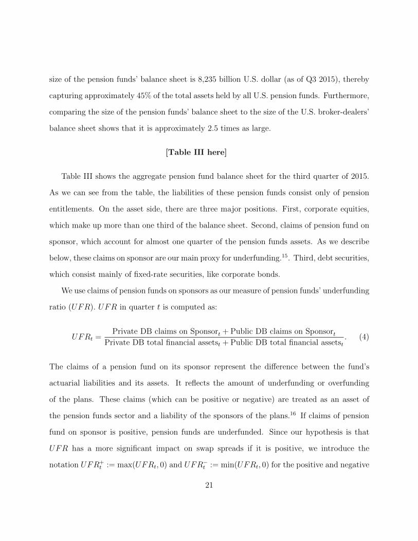
size of the pension funds’ balance sheet is 8,235 billion U.S. dollar (as of Q3 2015), thereby

capturing approximately 45% of the total assets held by all U.S. pension funds. Furthermore,

comparing the size of the pension funds’ balance sheet to the size of the U.S. broker-dealers’

balance sheet shows that it is approximately 2.5 times as large.

[Table III here]

Table III shows the aggregate pension fund balance sheet for the third quarter of 2015.

As we can see from the table, the liabilities of these pension funds consist only of pension

entitlements. On the asset side, there are three major positions. First, corporate equities,

which make up more than one third of the balance sheet. Second, claims of pension fund on

sponsor, which account for almost one quarter of the pension funds assets. As we describe

below, these claims on sponsor are our main proxy for underfunding.15. Third, debt securities,

which consist mainly of fixed-rate securities, like corporate bonds.

We use claims of pension funds on sponsors as our measure of pension funds’ underfunding

ratio (UFR). UFR in quarter t is computed as:

UFRt =Private DB claims on Sponsort + Public DB claims on Sponsort

Private DB total financial assetst + Public DB total financial assetst. (4)

The claims of a pension fund on its sponsor represent the di↵erence between the fund’s

actuarial liabilities and its assets. It reflects the amount of underfunding or overfunding

of the plans. These claims (which can be positive or negative) are treated as an asset of

the pension funds sector and a liability of the sponsors of the plans.16 If claims of pension

fund on sponsor is positive, pension funds are underfunded. Since our hypothesis is that

UFR has a more significant impact on swap spreads if it is positive, we introduce the

notation UFR

+t := max(UFRt, 0) and UFR

�t := min(UFRt, 0) for the positive and negative

21

part of the underfunding ratio respectively. Since we are using changes in UFR in our

regression analysis, we also introduce the notation �UFR

+t := (UFRt �UFRt�1) {UFRt>0}

and �UFR

�t := (UFRt � UFRt�1) {UFRt0}. Note that the way we define �UFR

+t means

that the measure includes a change from fully funded to underfunded periods but not from

underfunded to fully-funded periods (this change is included in �UFR

�t ).

B. Swap Spreads in Di↵erent Underfunding Regimes

It should be noted that for the end of quarter t, the Fed’s financial accounts of the U.S.

report the pension sponsors’ funding status resulting from events during the end-quarter

t � 1 to end-quarter t. This is reported roughly 2 weeks after end of quarter t. The swap

spreads that we use in the paper are calculated precisely at the end of quarter t. In this sense

our measure of funding status for quarter end t, UFRt, which is based on the information

from end-quarter t � 1 to end-quarter t is e↵ectively a lagged measure relative to the time

at which the swap spreads are collected.

Using the UFR measure constructed above, we provide some preliminary evidence on

the proposition that the demand by a significant subset of pension sponsors to receive fixed

in long-term swaps has an e↵ect on long-term swap spreads.

[Figure 2 here]

The top panel of Figure 2 shows a scatter plot of the 30-year swap spreads in basis

points against our measure of aggregate funding status, UFRt, and gives a first overview

of the results. The time period is between Q2 1994 and Q4 2015. The swap spreads are

quarter-end observations and we distinguish between the negative part (solid dots) and

positive part (circles) of the UFR, fitting a linear model with a di↵erent slope coe�cient in

22

the two regimes. The dashed lines indicate 95% confidence intervals. As we can see from

the top panel of Figure 2, the level of the swap spreads is negatively related to the UFR

for both funded and underfunded regions. In line with our theory, the slope coe�cient is

more negative in periods when pension funds are underfunded. The lower panel of Figure 2

shows the time series plot of the same variables, illustrating that both variables are relatively

volatile without an obvious trend component. The grey shaded areas indicate periods where

pension funds are fully funded or over-funded. The U.S. Economy was generating a surplus

during the end of this (shaded) period, with a drop in the supply of long-term government

bonds, which might have partially accounted for the increase in swap spreads. The stock

market boom during this period could have partially accounted for the over-funded status

of the pension plans.

The evidence presented in this section helps to motivate why the funding status of pension

plans, as suggested by our theory, may be a channel that could be at work in driving the

swap spreads down to negative levels. We next use regression analysis to further explore this

channel.

C. Regression Analysis

To shed additional light on the relationship between UFR and swap spreads we next run

a regression analysis of changes in 30-year swap spreads on changes in UFR.

17 Motivated by

the hedging strategy described in Section II.B.2, we control for the change in the di↵erence

between the 3-months Libor rate and 3-month general collateral repo rate (�LR spreadt)

in all regression specifications. Panels (1) and (2) of Table IV show that, without additional

control variables, pension fund underfunding is a significant explanatory variable for 30-year

swap spreads.

23

[Table IV here]

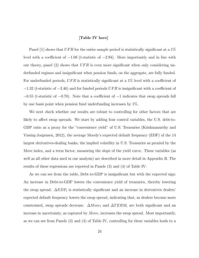
Panel (1) shows that UFR for the entire sample period is statistically significant at a 1%

level with a coe�cient of �1.08 (t-statistic of �2.94). More importantly and in line with

our theory, panel (2) shows that UFR is even more significant when only considering un-

derfunded regimes and insignificant when pension funds, on the aggregate, are fully funded.

For underfunded periods, UFR is statistically significant at a 1% level with a coe�cient of

�1.32 (t-statistic of �3.46) and for funded periods UFR is insignificant with a coe�cient of

�0.55 (t-statistic of �0.78). Note that a coe�cient of �1 indicates that swap spreads fall

by one basis point when pension fund underfunding increases by 1%.

We next check whether our results are robust to controlling for other factors that are

likely to a↵ect swap spreads. We start by adding four control variables, the U.S. debt-to-

GDP ratio as a proxy for the “convenience yield” of U.S. Treasuries (Krishnamurthy and

Vissing-Jorgensen, 2012), the average Moody’s expected default frequency (EDF) of the 14

largest derivatives-dealing banks, the implied volatility in U.S. Treasuries as proxied by the

Move index, and a term factor, measuring the slope of the yield curve. These variables (as

well as all other data used in our analysis) are described in more detail in Appendix B. The

results of these regressions are reported in Panels (3) and (4) of Table IV.

As we can see from the table, Debt-to-GDP is insignificant but with the expected sign:

An increase in Debt-to-GDP lowers the convenience yield of treasuries, thereby lowering

the swap spread. �EDFt is statistically significant and an increase in derivatives dealers’

expected default frequency lowers the swap spread, indicating that, as dealers become more

constrained, swap spreads decrease. �Movet and �TERMt are both significant and an

increase in uncertainty, as captured by Move, increases the swap spread. Most importantly,

as we can see from Panels (3) and (4) of Table IV, controlling for these variables leads to a

24

small drop in the statistical and economic significance of UFR, but leaves our main result

unchanged. Panel (3) shows that UFR for the full sample period is still significant at a 5%

level with a coe�cient of �0.96 (t-statistic of �2.19). More importantly, Panel (4) shows

that UFR during times of underfunding is still statistically significant at a 1% level with a

coe�cient of �1.27 (t-statistic of �3.18).

In panels (5) and (6) we add three more sets of control variables to check whether our

results remain robust to including more potential drivers of swap spreads. The first set

of control variables consists of the smoothed U.S. recession probabilities, as estimated by

Chauvet and Piger (2008), and two versions of the economic policy uncertainty (EPU) index,

constructed by Baker, Bloom, and Davis (2016) – uncertainty about the U.S. debt ceiling

and uncertainty about government spending. These variables can be viewed as proxies for

credit risk of the U.S. and could therefore a↵ect swap spreads through a higher treasury yield.

The second set of control variables include the mortgage refinancing rate and the amount

of U.S. agency MBS outstanding.18 These variables proxy for the impact of MBS duration

hedging on swap spreads. The last set of controls consists of the level of the 30-year treasury

yield, the broker-dealer leverage factor by Adrian, Etula, and Muir (2014), the VIX index,

and the 10-year on-the-run o↵-the-run spread, which could, in theory, also impact swap

spreads. Out of all these additional control variables, only the version of the EPU index

that captures uncertainty about the debt ceiling is statistically significant. We do not report

the coe�cient estimates for the additional insignificant variables for brevity and note that

adding these additional control variables only leads to a minor increase in the explanatory

power of our model (compared to specifications (3) and (4)). More importantly, adding these

controls leads to a minor drop in the statistical and economical significance of �UFR

+t , but

leaves our main results intact. Interestingly, the coe�cient on log(EPU

DebtCeilt ) is positive,

25

indicating that concerns about the U.S. debt ceiling tend to widen swap spreads.

As a next step, we check whether UFR is a significant explanatory variable for swap

spreads with shorter maturities. To that end, we regress changes in the 2-year, 5-year,

10-year, and 30-year swap spread on the positive and negative part of changes in UFR,

controlling for changes in the Libor-repo spread.19 The results of this regression are exhibited

in Table V. In line with our theory, UFR

+ is only significant for the 30-year swap spread

and insignificant for swap spreads with shorter maturities. We note that, in line with the

hedging argument from Section II.B.2, the Libor-repo spread is a significant explanatory

variable for swap spreads with shorter maturities (2-year and 5-year).

[Table V here]

In addition, we note that UFR is also a significant explanatory variable for 20-year swap

spreads and that the results for 20-year swap spreads are qualitatively similar to those for

30-year swap spreads, reported above. However, since the 20-year tenor is not a common

maturity for IRS and because, unlike the other tenors used in this section, the 20-year swap

spread needs to be computed using o↵-the-run bond yields, we relegate the discussion of

20-year swap spreads to Internet Appendix A.

D. Two-Stage Least Squares Regression Results

One concern about using UFR as an explanatory variable for swap spreads is that similar

factors can a↵ect both variables. For example, a decrease in the level of the yield curve

can simultaneously a↵ect swap spreads and the level of pension funds’ underfunding (which

would increase because the present value of the funds’ liabilities is computed using long-term

interest rates). To mitigate these concerns, we next run a 2-stage least squares regression.

26

In a first stage, we regress �UFRt on U.S. stock returns proxied by the excess return on the

CRSP value-weighted portfolio. In panels (2), (4), and (6) we drop fully funded periods and

only regress �UFR

+t on stock returns. Stock returns a↵ect UFR since pension funds are

heavily invested in corporate equity (almost half their assets are invested in corporate equity

according to Table III) and therefore decreasing stock returns increase UFR. At the same

time, there is no obvious connection between the 30-year swap spread and stock returns.

[Table VI here]

We therefore argue that the exclusion restriction is fulfilled. Furthermore, the results

from a weak instrument test give a p–value far below 0.1% for all six regression specifications,

suggesting that stock returns are not a weak instrument. In addition, the results from a Wu-

Hausman test give a p–value above 0.17 (ranging from 0.751 for specification (1) to 0.170

for specification (6)) for all six specifications. Hence, we cannot reject the over-identifying

restrictions.

Table VI shows the results of the second stage, where we use the projected UFR as

explanatory variable. Overall the results from the second stage are similar to those from

the OLS regression discussed before. The projected UFR is significant at a 1% level and

decreases in significance as we add controls. More importantly, the projected underfunded

ratio in regimes when pension funds are underfunded is even more significant (t-statistic

of �3.30 without controls) and remains significant even after adding our four main control

variables (t-statistic of �2.75).

27

E. Robustness Tests

To test the robustness of our results, we first note that we view our regression specifica-

tion (4) in Table IV as our main result and therefore focus on testing di↵erent variations of

this specification. We start by adding two di↵erent control variables to our analysis: CDS

premiums on the U.S. treasury and U.S. corporate bond issuance.20 We omit these variables

in our main tests because they are not available for the entire sample period and therefore

lower the total number of available observations. Moreover, as noted by Klingler and Lando

(2016), CDS premiums of safe countries do not necessarily reflect credit risk and can be

a↵ected by other variables, such as dealer banks’ financial constraints and regulatory vari-

ables. We therefore view the control variables in Panels (5) and (6) of Table IV as better

suited for testing the impact of U.S. credit risk on swap spreads.

[Table VII ahere]

As we can see from Panel (1) of Table VII, controlling for U.S. CDS premiums lowers the

significance of �UFR

+t but the CDS premiums themselves are not a significant explanatory

variable. Panel (2) of Table VII shows that controlling for U.S. corporate bond issuance does

not lower the significance of �UFR

+t and that corporate bond issuance is an insignificant

explanatory variable for 30-year swap spreads, but tends to lower the swap spread.

Next, we investigate the e↵ect of UFR on swap spreads in di↵erent sample periods. One

potential concern could be that a significant spike in UFR coincided with a significant drop

in swap spreads when Lehman Brothers defaulted and that the impact of UFR on swap

spreads could therefore purely be a post-crisis e↵ect. To address this concern, we add a

dummy slope variable that is equal to zero before Q3 2008 and equal to �UFRt from Q3

2008 on. As we can see from Panel (3) of Table VII, this dummy slope variable is not

28

statistically significant. We also investigate the impact of UFR on swap spreads in the

subsequent years of the default of Lehman Brothers. To that end, we add three di↵erent

dummy slope variables: The first one is equal to �UFRt from Q3 2008 to Q2 2009 and zero

in all other quarters. Similarly, the second and the third dummy slope variables are equal

to �UFRt from Q3 2009 to Q2 2010 and from Q3 2010 to Q2 2011, respectively, and zero

in all other quarters. As we can see from the table, the e↵ect of UFR on swap spreads is

almost twice as large during the year after the default of Lehman Brothers. This is in line

with our theory that the demand for duration by underfunded pension plans in combination

with constrained derivatives dealers drove swap spreads negative. Moreover, UFR is still a

significant explanatory variable for swap spreads over the entire period and the dummy slope

variables for the years after the default of Lehman Brothers are not statistically significant.

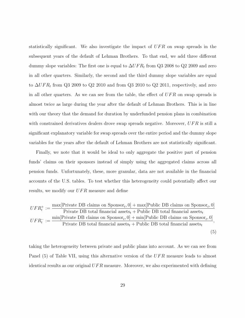
Finally, we note that it would be ideal to only aggregate the positive part of pension

funds’ claims on their sponsors instead of simply using the aggregated claims across all

pension funds. Unfortunately, these, more granular, data are not available in the financial

accounts of the U.S. tables. To test whether this heterogeneity could potentially a↵ect our

results, we modify our UFR measure and define

UFR

+t :=

max[Private DB claims on Sponsort, 0] + max[Public DB claims on Sponsort, 0]

Private DB total financial assetst + Public DB total financial assetst

UFR

�t :=

min[Private DB claims on Sponsort, 0] + min[Public DB claims on Sponsort, 0]

Private DB total financial assetst + Public DB total financial assetst,

(5)

taking the heterogeneity between private and public plans into account. As we can see from

Panel (5) of Table VII, using this alternative version of the UFR measure leads to almost

identical results as our original UFR measure. Moreover, we also experimented with defining

29

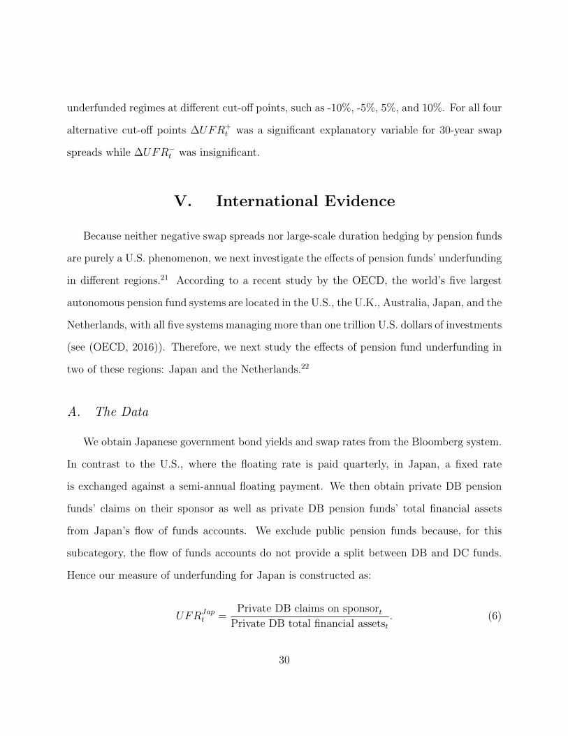
underfunded regimes at di↵erent cut-o↵ points, such as -10%, -5%, 5%, and 10%. For all four

alternative cut-o↵ points �UFR

+t was a significant explanatory variable for 30-year swap

spreads while �UFR

�t was insignificant.

V. International Evidence

Because neither negative swap spreads nor large-scale duration hedging by pension funds

are purely a U.S. phenomenon, we next investigate the e↵ects of pension funds’ underfunding

in di↵erent regions.21 According to a recent study by the OECD, the world’s five largest

autonomous pension fund systems are located in the U.S., the U.K., Australia, Japan, and the

Netherlands, with all five systems managing more than one trillion U.S. dollars of investments

(see (OECD, 2016)). Therefore, we next study the e↵ects of pension fund underfunding in

two of these regions: Japan and the Netherlands.22

A. The Data

We obtain Japanese government bond yields and swap rates from the Bloomberg system.

In contrast to the U.S., where the floating rate is paid quarterly, in Japan, a fixed rate

is exchanged against a semi-annual floating payment. We then obtain private DB pension

funds’ claims on their sponsor as well as private DB pension funds’ total financial assets

from Japan’s flow of funds accounts. We exclude public pension funds because, for this

subcategory, the flow of funds accounts do not provide a split between DB and DC funds.

Hence our measure of underfunding for Japan is constructed as:

UFR

Japt =

Private DB claims on sponsortPrivate DB total financial assetst

. (6)

30

Quarterly data on the funding status of DB pension funds are available from Q1 2005. Panel

A of Table VIII provides summary statistics for UFR

Japt as well as 30-year swap spreads.

As we can see from the table, Japanese pension funds have been underfunded during the

entire sample period. Moreover, the maximum level of UFR

Japt exceeds the maximum level

of UFRt in the U.S. by almost 10%. The higher underfunded ratio of Japanese pension funds

relative to the U.S. is not surprising, given that Japanese pension funds have been dealing

with decreasing interest rates and falling stock prices for much longer than U.S. pension

funds. Similarly to the U.S., Japanese pension funds try to avoid forcing their sponsors to

cover losses and the usage of swaps is explicitly permitted for these funds.

[Table VIII here]

When investigating the impact of pension funds’ underfunding on swap spreads for the

Netherlands, we define swap spreads as the di↵erence between the Euribor swap rate and

the yield of German government bonds in our main analysis and use swap spreads relative

to the yield of Dutch government bonds as a robustness check. We obtain swap rates and

government bond yields from the Bloomberg system. Data for the funding status of Dutch

DB pension funds are available on the DNB website, which provides data for “Liquid assets at

funds’ risk” and “Estimated technical provision at funds’ risk” from Q1 2007 on. According

to the Dutch pension fund regulation, a pension fund is underfunded if the ratio between the

two variables drops below 105%. In that case, a plan needs to provide a proposal of how to

become fully funded in the future to the Dutch supervisory authority and needs to lower the

overall risk of its portfolio, which is mainly done by reducing interest rate risk.23 Based on

these arguments, we first calculate the funding gap of Dutch pension funds as the di↵erence

between 1.05 times the estimated technical provision at funds’ risk and liquid assets at funds’

31

risk. We then construct UFR

Netht as follows:

UFR

Netht =

Funding gapt

Liquid assets at funds’ riskt. (7)

Finally, as we did for the U.S., we split the measure into a positive part, which corresponds

to times when pension funds are not underfunded and negative part that captures pension

funds’ underfunding. Panel B of Table VIII provides summary statistics for the Dutch UFR

measure as well as 30-year swap spreads relative to German government bonds and relative

to Dutch government bonds. As we can see from the table, Dutch pension funds are rarely

underfunded with a total of 12 underfunding observations.24

B. Results

We next test the relationship between swap spreads and UFRt for Japan and the Nether-

lands. To that end, we regress changes of 2-year, 5-year, 10-year, and 30-year swap spreads

on the �UFR

+t and �UFR

�t . In Japan, pension funds have been underfunded for the entire

sample period and we therefore drop �UFR

�t from the regression. Furthermore, we add the

6-month Libor-Repo spread as a control variable for Japan and do not control for changes

in the Libor-Repo spread in Europe due to limited data availability.

As we can see from Panel A of Table IX, �UFR

+t is a significant explanatory variable for

10-year and 30-year Japanese swap spreads but not for swap spreads with shorter maturities.

Both the statistical and economic significance of �UFR

+t are higher for 30-year swap spreads

than for 10-year swap spreads. Note that �UFR

+t is an even more significant explanatory

variable for Japanese 30-year swap spreads than for the U.S. Hence, we provide additional

results for Japan in the internet appendix. Analogous to the results for Japan, Panel B of

32

Table IX shows that, for the Netherlands, �UFR

+t is a significant explanatory variable for

30-year swap spreads (measured relative to German and Dutch government bond yields) and

insignificant for swap spreads with shorter maturities.

[Table IX here]

VI. Conclusion

We provide a novel explanation of persistent negative 30-year swap spreads, which is based

on the funding status of DB pension plans and the swap dealers’ balance sheet constraints.

Specifically, we argue that under-funded pension plans prefer to meet the duration needs

arising from their unfunded pension liabilities through receiving fixed payments in 30-year

interest rate swaps, instead of using levered positions in bonds. Swap dealers, who face

balance-sheet constraints, require a compensation in the form of negative swap spreads to

meet this demand. We present empirical evidence, which supports the view that the under-

funded status of DB pension plans has a significant explanatory power for 30-year swap

spreads, even after controlling for several other drivers of swap spreads, commonly used in the

swap literature. Moreover, we show that the funding status does not have any explanatory

power for swap spreads associated with shorter maturities between 2 and 10 years. We

present fairly consistent empirical evidence from the United States, Japan and Netherlands.

33

Appendix A. Model and Proofs

According to Equation (1), the dynamics of the swap PV are given as dPV (S) = cdP. To

derive a simple expression for the negative swap spread, we take the dynamics of the consol

bond as exogenously given and focus on market clearing in the swap market only. As in our

general analysis, we model the swap spread as a flow cost � 0 that the fixed receiver of

the swap pays in addition to the risk-free rate.

To keep the model tractable, we assume a static setup in which the pension fund is

minimizing its future underfunding with risk aversion � :25

minm,n

[E[F ] +�

2V ar(F )] (A1)

The dynamics of F are given as:

dF = (L�m� nc)dP + (r � �)dt+ (r + �)(mP + n(cP � 1)� A)dt,

where we implicitly assume mP +n(cP �1)�A � 0 (otherwise the fund would invest money

at the risk-free rate and receive a return r + � instead of r).

The swap dealers decide on the swap supply based on the following mean-variance opti-

mization problem:

maxs

hrW � s� � a

2

�s

2�

2�i

, (A2)

where we assume that dealers associate no risk premium to trading swaps. The interpretation

of the risk-aversion a is that dealers face balance sheet constraints and even a hedged position

in an IRS requires balance sheet. In this model setup, the amount of balance sheet consumed

34

by a new swap position is proportional to the variance of the swap’s mark-to-market value.

The coe�cient a can therefore be interpreted as the tightness of the dealers’ balance sheet

constraint. For a = 0, the dealer is unconstrained and would supply swaps at the fair swap

spread � = 0. Proposition 2 characterizes the equilibrium swap spread in our setting.

Equilibrium in our model is defined as a situation where pension funds solve problem

(A1), derivatives dealers solve problem (A2), and the interest rate swap market clears.

Proof of Proposition 1

Plugging µP and �P into Equation (A1), the fund’s optimization problem simplifies to:

minm,n

h(LP �mP � n)µP +

�

2(LP �mP � n)2�2

P + [n(r � �) + (r + �) (mP � A)]i, (A3)

where the first two terms are the mean and the variance of the underfunding and the last

term represents the sum of the costs of using swaps and the cost of using direct leverage.

Taking the FOC of Equation (A3) gives:

@

@m

:� PµP + (r + �)P � �P (LP �mP � n)�2P

!= 0

@

@n

:� µP � (� � r)� �(LP �mP � n)�2P

!= 0

Because swaps and bonds are perfectly correlated, we start by considering the following

three corner solutions. First, if the pension fund only uses consols and pays the short-selling

cost �, then his optimal allocation to consols is given as:

mP = LP +µP � r

��

2P

� �

��

2P

35

and the value function is:

(r + �)F � 1

2

(µP � (r + �))2

��

2P

. (A4)

Second, if the pension fund only uses its available funding to purchase bonds, it invests

mP = A in bonds and the value function is:

FµP +�

2F

2�

2P . (A5)

Third, if the fund allocates its maximum available funding to consols, that is, it invests

mP = A in consols, and chooses the optimal allocation n

⇤ to swaps. Then, n⇤ is given as:

n = F +µP � (r � �)

��

2P

and the value of its minimization problem is:

F (r � �)� 1

2

(µP � (r � �))2

��

2P

(A6)

Comparing Equations (A4) and (A6) we can see that �� < � is a su�cient condition for

the pension fund to prefer swaps over consols. Comparing Equations (A5) and (A6), we find

that the fund prefers using swaps over not hedging if:

F (µP � r) +�

2F

2�

2P � ��F � 1

2

(µP � (r � �))2

��

2P

.

Hence, a su�cient condition for the pension fund to hedge is given as � � �(µP � r) ��2F�

2P and, under the assumptions in Proposition 1, the corner solution where the pension

36

fund uses swaps is preferred over the other two corner solutions.

To ensure that m⇤ = A/P and n

⇤ = F + µP�(r��)��2

Pare indeed the optimal investments for

the pension fund, we plug m

⇤ = (A � x)/P and n

⇤ = F + µP�(r����2

P+ y into Equation (A1).

For x 0, the solution to the minimization problem is:

F (r � �)� 1

2

(µP � (r � �))2

��

2P

� x(�+ �) +�

2�

2P (x� y)2. (A7)

By assumption, � + � > 0 and because � 0 we assumed x 0, the term �x(� + �) is

minimized for x = 0. With x = 0, the last term simplifies to �2�

2Py

2, which is minimized for

y = 0. Analoguously, for x � 0, the we need to set � = 0 in equation (A7) and, again, the

expression is minimized for x = y = 0. ⌅

Proof of Proposition 2

The supply of swaps can be derived from Equation(A2):

s = � �

a�

2. (A8)

We first assume that the pension fund’s demand for swaps is given by Equation (2), which

leads to the equilibrium swap spread in Equation (3).

With that, we can show that, for a < �, the equilibrium swap spread satisfies the hedging

condition stated in Proposition 1, which completes the proof. ⌅

Appendix B. Data Description

This appendix provides additional details about the data used for our analysis.

37

1. Swap Spreads: Swap rates and government bond yields for 2, 3, 5, 10, and 30 years

to maturity are obtained from the Bloomberg system. The swap rates are the fixed

rates an investor would receive on a semi-annual basis at the current date in exchange

for quarterly Libor payments. The U.S. treasury yields are the yields of the most

recently auctioned issue and adjusted to reflect constant time to maturity. For 3-year

and 7-year treasury yields, we supplement the Bloomberg data with treasury yields

from the FED H.15 reports due to several missing observations in the Bloomberg data.

Swap spreads are computed as the di↵erence between swap rate and treasury yield,

where the swap rate is adjusted to reflect the di↵erent daycount conventions which are

actual/360 for swaps and actual/actual for treasuries.

2. Underfunded Ratio (UFR) : For the U.S., quarterly data on two types of defined

benefit (DB) pension plans, private as well as public local government pension plans,

are obtained from the financial accounts of the U.S. (former flow of funds) tables

L.118b and L.120b. UFR in quarter t is then computed using Equation (4). Next,

positive and negative part are defined as UFR

+t := max(UFRt, 0) and UFR

�t :=

min(UFRt, 0). Changes in UFR in the di↵erent regimes are computed as �UFR

+t :=

(UFRt�UFRt�1) {UFRt>0} and (�UFR

�t := (UFRt�UFRt�1) {UFRt0}. For Japan,

we obtain DB pension funds’ claims on sponsor as well as total financial assets from

Japan’s flow of funds tables. For the Netherlands, we collect data on “liquid assets

at the funds’ risk” and “estimated technical provision at funds’ risk’ from the Dutch

central banks’ website and construct the UFR proxy according to Equation 7.

3. Libor-repo spread: For the U.S., the 3-month Libor rate as well as the 3-month

general collateral repo rate are obtained from the Bloomberg system. Similarly, for

Japan, the 6-months general collateral repo rate and the 6-months JPY Libor rate are

38

obtained from Bloomberg. The Libor-repo spread is then computed as the di↵erence

between these two variables.

4. Debt-to-GDP ratio: Quarterly data on the U.S. debt-to-GDP are obtained from the

federal reserve bank of St. Louis which provides a seasonally-adjusted time series.

5. Broker-Dealer EDF: Expected default frequencies are provided by Moody’s analytics

and we use the equally-weighted average of the 14 largest derivatives-dealing banks

(G14 banks). These 14 banks are: Morgan Stanley, JP Morgan, Bank of America,

Wells Fargo, Citigroup, Goldman Sachs, Deutsche Bank, Societe Generale, Barclays,

HSBC, BNP Paribas, Credit Suisse, Royal Bank of Scottland, and UBS.

6. Move Index: The Move index is computed as the 1-month implied volatility of U.S.

treasury bonds with 2,5,10, and 30 years to maturity. Index levels are obtained from

the Bloomberg system.

7. Term Factor: This factor captures the slope of the yield curve, measured as the di↵er-

ence between the 30-year treasury yield and the 3-month treasury yield. A description

of these yields can be found under point 1 (swap spreads).

8. Level: The level of the yield curve is captured by the 30-year treasury yield. For a

description of this yield see point 1 (swap spreads).

9. VIX: Is the implied volatility of the S&P 500 index and data on VIX are obtained

from the Bloomberg System.

10. On-the-run spread: The spread is computed for bonds with 10-years to maturity

because estimates of the 30-year spread are noisy and su↵er from the 2002-2005 period

where the U.S. treasury reduced its debt issuance. The 10-year on-the-run yield is

obtained from the FED H.15 website and the 10-year o↵-the-run yield is constructed

as explained in Gurkaynak, Sack, and Wright (2007) and data are obtained from http:

39

//www.federalreserve.gov/pubs/feds/2006.

11. Broker-Dealer Leverage: This variable captures the leverage of U.S. broker-dealers

and is described in more detail in Adrian et al. (2014). Until Q4 2009, data on this

variable are obtained from Tyler Muir’s website. Since the data ends in Q4 2009, we

use the financial accounts of the U.S. data, following the procedure described in Adrian

et al. (2014) to supplement the time series with more recent observations for the Q1

2010 – Q4 2015 period.

12. Mortage Refinancing: Quarterly mortgage origination estimates are directly ob-

tained from the Mortgage Bankers Association website. We use mortgage originations

due to refinancing as a proxy for the mortgage refinancing rate.

13. U.S. stock market returns: The U.S. stock returns are quarterly returns of the

CRSP value-weighted portfolio in excess of the risk-free rate and obtained from Ken-

neth French’s website.

14. CDS premiums on the U.S. treasury: The U.S. CDS premiums are 5-year CDS

premiums of Euro-denominated CDS contracts (which are the most liquidly traded

CDS contracts on the U.S. treasury). The data are obtained from Markit.

15. MBS Outstanding: These are the total amount of U.S. agency MBS outstanding.

The data are obtained from SIFMA website.

16. Corporate bond issuance: The quarterly issuance of all U.S. investment grade and

non-investment grade bonds were provided to us courtesy to SIFMA.

17. EPU data: We use two categories of the economic policy uncertainty (EPU) index,

proposed by Baker et al. (2016). These two categories are “government spending” and

“debt ceiling” and available under www.policyuncertainty.com

18. U.S. recession probabilities These are the smoothed recession probabilities, es-

40

timated in Chauvet and Piger (2008). The data are obtained from Jeremy Piger’s

website.

Notes

1The leverage implications of IRS on pension sponsors are not investigated in this paper.

2See, for instance, https://self-evident.org/?p=780.

3See, for instance, Van Deventer (2012).

4Another factor that should contribute to the positive level of swap spreads is that the

income from holding treasuries is not taxable for state income tax, while income related to

the Libor rate typically is (see Elton, Gruber, Agrawal, and Mann, 2001). This “tax spread”

could be an additional reason for the high level of swap spreads before the financial crisis

and makes the negative swap spread even more surprising.

5The prolonged drop in interest rates, following the crisis of 2008, increased the duration

of pension liabilities and the monetary policy of the Fed also might have contributed to the

overall drop in other interest rates and spreads.

6In this analysis, we also include swap spreads with 7 years and 20 years to maturity.

Data for these maturities are obtained from the FED H.15 website.

7This number is a first approximation that we obtained from http://www.cmegroup.com/

clearing/financial-and-collateral-management/. They analyze haircuts for securities

posted as collateral in cleared derivatives transactions. However, market participants confirm

that 6% is a reasonable proxy for haircuts of Treasuries with 30 years to maturity.

8There may be other frictions such as taxes that may also favor IRS relative to repo. In the

U.S., Internal Revenue Service views repo as financing that would subject the pension plan

41

to tax filings as Unrelated Business Income (UBI). Most U.S. pension plans will therefore

avoid UBI taxes by avoiding repo and relying on IRS, which does not invoke UBI taxes. We

thank Scott McDermott for alerting us to this point.9See http://www.bloomberg.com/apps/news?pid=newsarchive&sid=aUq.d1dYuhEA

10These surveys are available under http://www.ai-cio.com/surveys/.

11Feldhutter and Lando (2008) argue that using IRS is the predominant way for doing this

as opposed to using Treasuries.

12Insurance companies could be another big demander for receiving the fixed rate in long-

term swaps, but we have no data available to characterize their funding status. In addition to

insurance companies, recent long-term corporate bond issuance might also create a demand

for receiving fixed in long-dated interest rate swaps. This is because companies may hedge

the duration risk of their bond issuance.

13We provide further details about this hedging strategy in Table IA.4 in the internet

appendix.

14Another friction we abstract away from in this discussion is the possible presence of credit

risk in U.S. Treasuries. The reason for doing so is that it is not obvious how an increase in

credit risk in U.S. Treasuries might a↵ect the swap spread. Clearly, an increase in treasury

credit risk would increase the treasury yield and assuming all else equal, a decrease in the

swap spread would result. However, it is not obvious that swap rates would be una↵ected by

the increase in treasury credit risk since interbank lending rates would presumably increase

sharply when U.S. credit risk increases. Therefore, it is just as likely that the swap rate

would be elevated.

15The Financial Accounts report assets and liabilities (and corresponding financial flows)

for both private and public DB pension funds. Prior to September 2013, the assets and

42

liabilities of DB pension plans were reported using cash accounting principles, which record

the revenues of pension funds when cash is received and expenses when cash is paid out.

Under this treatment, there was no measure of a plan’s accrued actuarial liabilities. Rather,

the liabilities in the Financial Accounts were set equal to the plans’ assets. As a result,

the Financial Accounts did not report any measure of underfunding or overfunding of the

pension sector’s actuarial liabilities, as would occur if the assets held by the pension sector fell

short of or exceeded the liabilities. Starting with the September 2013 release, the Financial

Accounts treat DB pensions using accrual accounting principles, whereby the liabilities of

DB pension plans are set equal to the present value of future DB benefits that participants

have accumulated to date, which are calculated using standard actuarial methods. This new

measure is retroactively made available. Throughout, we use the accrual measures of the

claims of pension funds on sponsors.

16See Stefanescu and Vidangos (2014) for further details.

17We use changes in these variables since both are highly serially correlated. A regression

of the level of the 30-year swap spread (level of UFR) on the lagged level of the 30-year

swap spread (UFR) gives a highly significant coe�cient of 0.95 (0.97).

18Two other control variables that we do not add to this regression are the U.S. agency

MBS issuance and the total amount of all IRS outstanding. Unfortunately, these data are

only available at an annual and semi-annual frequency, respectively. In unreported robustness

checks, we used annual and semi-annual data and found that controlling for these variables

does not a↵ect the link between UFR and swap spreads.

19We focus on 2,5, 10, and 30-year swap spreads since there are no missing observations for

these data and we do not need to supplement them with data from the FED H.15 reports.

20According to SIFMA, the average maturity of newly issued bonds varied from 7.3 years

43

in the year 2000 to 17.0 in the year 2015. Hence, the issuance of long-dated corporate bonds

might generate a hedging demand for long-dated IRS by corporations.

21We thank the referees for suggesting this extension to international markets.

22Due to data constraints and the use of inflation-linked pension plans, we did not pursue

the pension schemes in Australia and the U.K.

23 As stated by Deutsche Bank markets research: “One of the major risks that Dutch

pension funds run is interest rate risk and hence their reduced ability to take risk could

on the margin increase receiving pressure [...] from the Durch pension fund community”

(Singhania, 2015).

24We only include data up until Q4 2014 because from Q1 2015, the policy funding ratio

is not based on the current ratio between assets and liabilities anymore but on the average

funding ratio over the past year.

25Note that this problem is equivalent to the pension fund maximizing its level of funding,

A� LP < 0, that is:

maxm,n

[E[A� LP ]� �

2V ar(A� LP )].

44

REFERENCES

Abad, Jorge, Inaki Aldasoro, Christoph Aymanns, Marco D’Errico, Linda Fache Rousova,

et al., 2016, Shedding light on dark markets: First insights from the new eu-wide otc

derivatives dataset, European Systemic Risk Board.

Adams, James, and Donald J Smith, 2009, Mind the gap: using derivatives overlays to hedge

pension duration, Financial Analysts Journal 65, 60–67.

Adrian, Tobias, Erkko Etula, and Tyler Muir, 2014, Financial intermediaries and the cross-

section of asset returns, Journal of Finance 69, 2557–2596.

Ang, Andrew, Bingxu Chen, and Suresh Sundaresan, 2013, Liability-driven investment with

downside risk, Journal of Portfolio Management 40, 71.

Baker, Scott R, Nicholas Bloom, and Steven J Davis, 2016, Measuring economic policy

uncertainty, Quarterly Journal of Economics 131, 1593–1636.

CGFS, 2011, Fixed income strategies of insurance companies and pension funds, Bank for

International Settlements, Committee on the Global Financial System.

Chauvet, Marcelle, and Jeremy Piger, 2008, A comparison of the real-time performance of

business cycle dating methods, Journal of Business & Economic Statistics 26, 42–49.

Chernenko, Sergey, and Michael Faulkender, 2012, The two sides of derivatives usage: Hedg-

ing and speculating with interest rate swaps, Journal of Financial and Quantitative Anal-

ysis 46, 1727–1754.

Collin-Dufresne, Pierre, and Bruno Solnik, 2001, On the term structure of default premia in

the swap and libor markets, Journal of Finance 56, 1095–1115.

45

Domanski, Dietrich, Hyun Song Shin, and Vladyslav Sushko, 2015, The hunt for duration:

not waving but drowning?, BIS Working Paper.

Duarte, Je↵erson, Francis A Longsta↵, and Fan Yu, 2007, Risk and return in fixed-income

arbitrage: Nickels in front of a steamroller?, Review of Financial Studies 20, 769–811.

Du�e, Darrell, and Kenneth J Singleton, 1997, An econometric model of the term structure

of interest-rate swap yields, Journal of Finance 52, 1287–1321.

Elton, Edwin J, Martin J Gruber, Deepak Agrawal, and Christopher Mann, 2001, Explaining

the rate spread on corporate bonds, Journal of Finance 56, 247–277.

Faulkender, Michael, 2005, Hedging or market timing? selecting the interest rate exposure

of corporate debt, Journal of Finance 60, 931–962.

Feldhutter, Peter, and David Lando, 2008, Decomposing swap spreads, Journal of Financial

Economics 88, 375–405.

Garleanu, Nicolae, and Lasse Heje Pedersen, 2011, Margin-based Asset Pricing and Devia-

tions from the Law of One Price, Review of Financial Studies 24, 1980–2022.

Garleanu, Nicolae, Lasse Heje Pedersen, and Allen M Poteshman, 2009, Demand-based

option pricing, Review of Financial Studies 22, 4259–4299.

Greenwood, Robin, and Dimitri Vayanos, 2010, Price pressure in the government bond

market, American Economic Review 585–590.

Grinblatt, Mark, 2001, An analytic solution for interest rate swap spreads, International

Review of Finance 2, 113–149.

46

Gromb, Denis, and Dimitri Vayanos, 2002, Equilibrium and welfare in markets with finan-

cially constrained arbitrageurs, Journal of Financial Economics 66, 361–407.

Gromb, Denis, and Dimitri Vayanos, 2010, Limits of Arbitrage, Annual Review of Financial

Economics 2, 251–275.

Gurkaynak, Refet S, Brian Sack, and Jonathan H Wright, 2007, The us treasury yield curve:

1961 to the present, Journal of Monetary Economics 54, 2291–2304.

Hanson, Samuel G, 2014, Mortgage convexity, Journal of Financial Economics 113, 270–299.

Jermann, Urban J, 2016, Negative swap spreads and limited arbitrage, Working paper,

Wharton School.

Jermann, Urban J, and Vivian Z Yue, 2013, Interest rate swaps and corporate default, ECB

Working Paper.

Johannes, Michael, and Suresh Sundaresan, 2007, The impact of collateralization on swap

rates, Journal of Finance 62, 383–410.

Klingler, Sven, and David Lando, 2016, Safe haven cds pemiums, Working Paper, Copen-

hagen Business School.

Krishnamurthy, Arvind, 2010, How debt markets have malfunctioned in the crisis, Journal

of Economic Perspectives 24, 3–28.

Krishnamurthy, Arvind, and Annette Vissing-Jorgensen, 2012, The aggregate demand for

treasury debt, Journal of Political Economy 120, 233–267.

Lang, Larry HP, Robert H Litzenberger, and Andy Luchuan Liu, 1998, Determinants of

interest rate swap spreads, Journal of Banking & Finance 22, 1507–1532.

47

Leising, Matthew, 2013, U.s. approves $ 6.8 trillion in pension funds for cleared swaps,

Bloomberg article.

Liu, Jun, and Francis A Longsta↵, 2004, Losing money on arbitrage: Optimal dynamic

portfolio choice in markets with arbitrage opportunities, Review of Financial Studies 17,

611–641.

Liu, Jun, Francis A Longsta↵, and Ravit E Mandell, 2006, The market price of risk in interest

rate swaps: the roles of default and liquidity risks, Journal of Business 79, 2337–2359.

Longsta↵, Francis A, 2004, The flight-to-liquidity premium in us treasury bond prices, Jour-

nal of Business 77, 511–526.

Lou, Wujiang, 2009, On asymmetric funding of swaps and derivatives-a funding cost expla-

nation of negative swap spreads, Working paper available at SSRN.

Musto, David, Greg Nini, and Krista Schwarz, 2014, Notes on bonds: Liquidity at all costs

in the great recession, Working paper, University of Pennsylvania.

OECD, 2016, Pension funds in figures, Research note, OECD.

Ring, Ed, 2014, Estimating americas total unfunded state and local government pension

liability, California Policy Centerr.

Shleifer, Andrei, and Robert W Vishny, 1997, The limits of arbitrage, Journal of Finance

52, 35–55.

Singhania, Abhishek, 2015, Dutch ufr curve adjustment, Deutsche Bank Markets Research.

48

Stefanescu, Irina, and Ivan Vidangos, 2014, Introducing actuarial liabilities and funding

status of defined-benefit pensions in the u.s. financial accounts, Technical report, FEDS

Notes.

Sundaresan, Suresh, and Fernando Zapatero, 1997, Valuation, optimal asset allocation and

retirement incentives of pension plans, Review of Financial Studies 10, 631–660.

Van Deventer, Donald R., 2012, Why is the 30 year swap spread to treasuries negative?,

Kamakura report.

Vasicek, Oldrich, 1977, An equilibrium characterization of the term structure, Journal of

Financial Economics 5, 177–188.

49

1995 1997 1999 2001 2003 2005 2007 2009 2011 2013 2015

−50

050

100

150

Basi

s Po

ints

Libo

r−R

epo

spre

ad tu

rns

nega

tive

Lehm

an2−year5−year10−year30−year

Figure 1. Term structure of interest rate swap spreads: The graph shows the history ofswap spreads (monthly averages) from May 1994 until December 2015. The grey shaded areasrepresent U.S. recession periods. The source for our data is Bloomberg. The di↵erences in marketconventions have been taken into account in computing the spreads

50

●●●

●●

●

●

●

●●

●

●●

●●●

●●

●

●

●●

●

●●

●●●

●

●●

●

●

●

●

●

●●●

● ●

●

●●

●

●

●●

●●

●●

●●●

●●●

●

●●

●

●

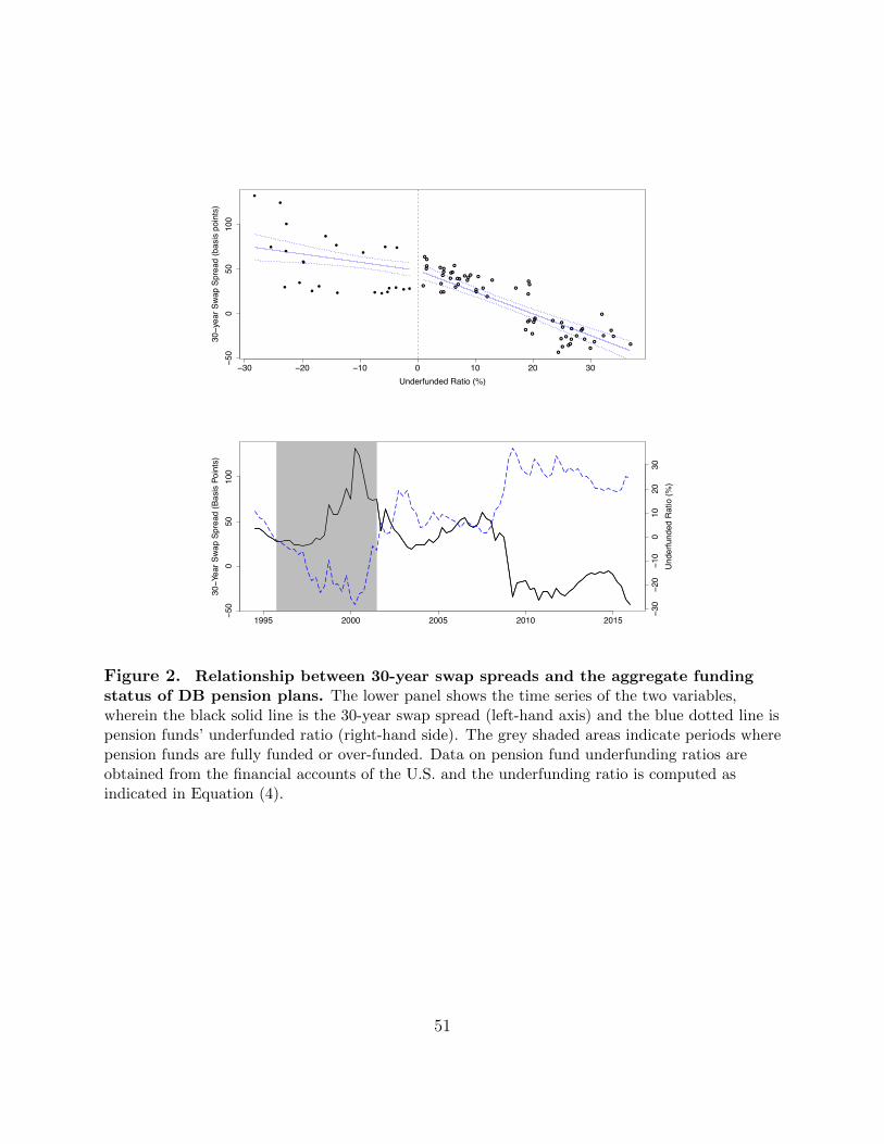
−30 −20 −10 0 10 20 30−50

050

100

Underfunded Ratio (%)

30−y

ear S

wap

Spre

ad (b

asis

poi

nts)

●●●●

●● ●●●

●●

●

●

●●

●

●

●

●

●

●

●●●

1995 2000 2005 2010 2015−50

050

100

30−Y

ear S

wap

Spre

ad (B

asis

Poi

nts)

−30

−20

−10

010

2030

Und

erfu

nded

Rat

io (%

)Figure 2. Relationship between 30-year swap spreads and the aggregate fundingstatus of DB pension plans. The lower panel shows the time series of the two variables,wherein the black solid line is the 30-year swap spread (left-hand axis) and the blue dotted line ispension funds’ underfunded ratio (right-hand side). The grey shaded areas indicate periods wherepension funds are fully funded or over-funded. Data on pension fund underfunding ratios areobtained from the financial accounts of the U.S. and the underfunding ratio is computed asindicated in Equation (4).

51

Table IOLS Regressions of Swap Spreads on Principal Components

For each of the two sub-periods, PC1 and PC2 are the first and second principal components ofthe term structure of swap spreads for this sub period. We use monthly treasury yields and swaprates from the Bloomberg system to compute swap spreads. 3-year and 7-year treasury data aresupplemented using data from the FED H15 reports. The sample period is May 1994 – December2015. � is the estimated loading on the respective PC.

Pre September 2008 Post September 2008

PC1 PC2 PC1 PC2

� R

2� R

2� R

2� R

2

2 yr 0.33 78.0% 0.41 18.2% 0.53 97.0% -0.03 0.1%3 yr 0.33 74.4% 0.46 23.1% 0.56 98.1% -0.01 0.0%5 yr 0.40 91.1% 0.26 6.0% 0.45 97.9% 0.04 0.2%7 yr 0.37 94.1% 0.16 2.8% 0.36 86.5% -0.14 2.8%10 yr 0.43 94.8% -0.14 1.7% 0.19 64.4% -0.26 24.8%20 yr 0.35 78.1% -0.42 17.3% -0.20 24.8% -0.71 70.2%30 yr 0.42 77.0% -0.57 21.5% 0.06 3.1% -0.64 85.6%

52

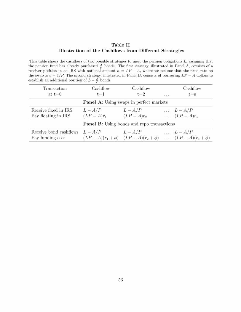
Table IIIllustration of the Cashflows from Di↵erent Strategies

This table shows the cashflows of two possible strategies to meet the pension obligations L, assuming thatthe pension fund has already purchased A

P bonds. The first strategy, illustrated in Panel A, consists of areceiver position in an IRS with notional amount n = LP � A, where we assume that the fixed rate onthe swap is c = 1/P. The second strategy, illustrated in Panel B, consists of borrowing LP � A dollors toestablish an additional position of L� A

P bonds.

Transaction Cashflow Cashflow Cashflowat t=0 t=1 t=2 . . . t=s

Panel A: Using swaps in perfect markets

Receive fixed in IRS L� A/P L� A/P . . . L� A/P

Pay floating in IRS (LP � A)r1 (LP � A)r2 . . . (LP � A)rs

Panel B: Using bonds and repo transactions

Receive bond cashflows L� A/P L� A/P . . . L� A/P

Pay funding cost (LP � A)(r1 + �) (LP � A)(r2 + �) . . . (LP � A)(rs + �)

53

Table IIIAggregate Pension Fund Balance Sheet as of Q3 2015

This table presents the assets and liabilities of private as well as state and local governmentemployee defined-benefit (DB) pension plans. The amounts are in billions of dollars, not seasonallyadjusted. (Source: Financial accounts of the United States)

DB Pension Fund Assets (billions) DB Pension Fund Liabilities

checkable deposits and currency $14.42 pension entitlements $8,430.73total time and savings deposits $75.67money market mutual fund shares $85.45security repurchase agreements $7.11debt securities $1,744.41commercial paper $82.26Treasury securities $365.19agency- and GSE-backed securities $191.15corporate and foreign bonds $1,101.75municipal securities $4.05total mortgages $20.00corporate equities $3,141.21mutual fund shares $613.29miscellaneous assets $2,533.58unallocated insurance contracts $58.02pension fund contributions receivable $47.28claims of pension fund on sponsor $2,044.53unidentified miscellaneous assets $383.76

TOTAL $8,235.12 TOTAL $8,430.73

54

Table IV30-Year Swap Spreads and Pension Fund Underfunding

This table reports results from regressions of quarterly changes in the 30-year swap spread on the indicatedvariables. �UFRt is the change in the underfunding ratio of private and local government defined ben-efit pension funds, as defined in Equation (4), �UFR

+t (�UFR

�t ) is the change in UFRt if UFRt > 0

(UFRt 0) and zero otherwise. �LR Spreadt is the change in the di↵erence between the 3-month Liborrate and 3-month General Collateral repo rate, �Debt/GDPt is the change in the ratio of U.S. public debt toGDP, �EDFt is the change in the Moody’s expected default frequency of the 14 largest derivatives-dealingbanks (G14 banks), �Movet is the change in the 1-month implied volatility of U.S. Treasuries with 2,5,10, and 30 years to maturity, �TERMt measures changes in the slope of the yield curve, approximated asthe di↵erence between 30-year and 3-month treasury yields, and log(EPU

DebtCeilt ) is a version of the policy

uncertainty index by Baker et al. (2016) that captures uncertainty about the debt ceiling. The additionalcontrols include changes in the following variables: the level of the 30-year treasury yield, the U.S. mortgagerefinancing rate, agency MBS outstanding, the VIX index, the 10-year on-the-run-o↵-the-run spread, U.S.recession probabilities, as well as the levels of the Adrian et al. (2014) broker-dealer leverage factor anduncertainty about government spending. All variables are quarter-end. The numbers in parenthesis areheteroskedasticity-robust t-statistics.⇤⇤⇤, ⇤⇤, and ⇤ indicate significance at a 1%, 5%, and 10% level respec-tively. The observation period is Q3 1994 – Q4 2015 with 5 missing observations between Q4 1997 and Q41998 due to missing repo rates.

(1) (2) (3) (4) (5) (6)

Intercept �1.14 �1.05 �0.59 �0.53 25.60⇤ 26.03⇤

(�0.91) (�0.85) (�0.41) (�0.37) (1.78) (1.78)

�UFRt �1.08⇤⇤⇤ �0.96⇤⇤ �0.68(�2.94) (�2.19) (�1.37)

�UFR

+t �1.32⇤⇤⇤ �1.27⇤⇤⇤ �1.19⇤⇤

(�3.46) (�3.18) (�2.40)

�UFR

�t �0.55 �0.47 �0.27

(�0.78) (�0.59) (�0.34)

�LR Spreadt 0.05 0.05 0.01 0.01 �0.04 �0.04(1.06) (1.21) (0.15) (0.22) (�0.52) (�0.53)

�Debt/GDPt �1.04 �0.96 �0.53 �0.40(�1.34) (�1.24) (�0.69) (�0.57)

�EDFt �0.05⇤⇤ �0.03 �0.07⇤ �0.06(�2.12) (�1.65) (�1.88) (�1.48)

�Movet 0.17⇤⇤ 0.17⇤⇤ 0.24⇤⇤ 0.23⇤⇤

(2.56) (2.58) (2.54) (2.37)

�TERMt �0.05⇤ �0.06⇤⇤ �0.06 �0.06(�1.76) (�2.00) (�1.38) (�1.43)

log(EPU

DebtCeilt ) 1.39⇤⇤ 1.42⇤⇤

(2.09) (2.10)

Add. Controls? No No No No Yes Yes

Observations 81 81 81 81 81 81Adjusted R2 0.15 0.15 0.27 0.28 0.28 0.29

55

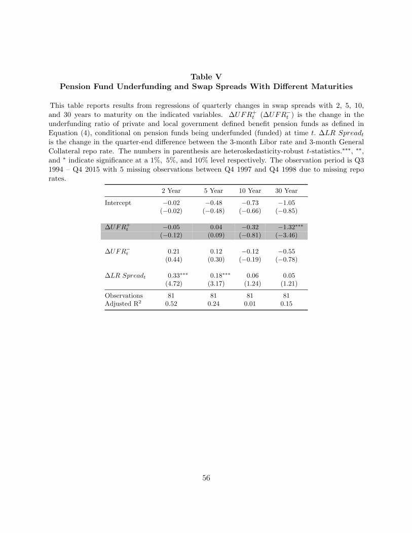
Table VPension Fund Underfunding and Swap Spreads With Di↵erent Maturities

This table reports results from regressions of quarterly changes in swap spreads with 2, 5, 10,and 30 years to maturity on the indicated variables. �UFR

+t (�UFR

�t ) is the change in the

underfunding ratio of private and local government defined benefit pension funds as defined inEquation (4), conditional on pension funds being underfunded (funded) at time t. �LR Spreadt

is the change in the quarter-end di↵erence between the 3-month Libor rate and 3-month GeneralCollateral repo rate. The numbers in parenthesis are heteroskedasticity-robust t-statistics.⇤⇤⇤, ⇤⇤,and ⇤ indicate significance at a 1%, 5%, and 10% level respectively. The observation period is Q31994 – Q4 2015 with 5 missing observations between Q4 1997 and Q4 1998 due to missing reporates.

2 Year 5 Year 10 Year 30 Year

Intercept �0.02 �0.48 �0.73 �1.05(�0.02) (�0.48) (�0.66) (�0.85)

�UFR

+t �0.05 0.04 �0.32 �1.32⇤⇤⇤

(�0.12) (0.09) (�0.81) (�3.46)

�UFR

�t 0.21 0.12 �0.12 �0.55

(0.44) (0.30) (�0.19) (�0.78)

�LR Spreadt 0.33⇤⇤⇤ 0.18⇤⇤⇤ 0.06 0.05(4.72) (3.17) (1.24) (1.21)

Observations 81 81 81 81Adjusted R2 0.52 0.24 0.01 0.15

56

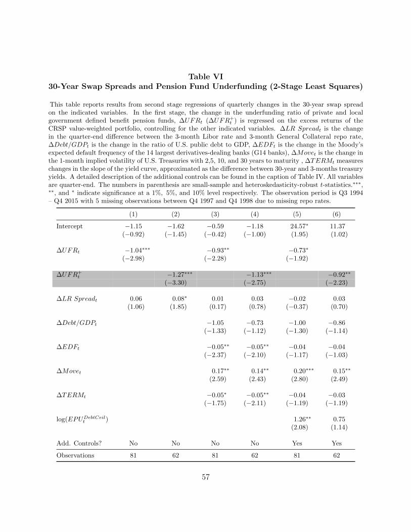
Table VI30-Year Swap Spreads and Pension Fund Underfunding (2-Stage Least Squares)

This table reports results from second stage regressions of quarterly changes in the 30-year swap spreadon the indicated variables. In the first stage, the change in the underfunding ratio of private and localgovernment defined benefit pension funds, �UFRt (�UFR

+t ) is regressed on the excess returns of the

CRSP value-weighted portfolio, controlling for the other indicated variables. �LR Spreadt is the changein the quarter-end di↵erence between the 3-month Libor rate and 3-month General Collateral repo rate,�Debt/GDPt is the change in the ratio of U.S. public debt to GDP, �EDFt is the change in the Moody’sexpected default frequency of the 14 largest derivatives-dealing banks (G14 banks), �Movet is the change inthe 1-month implied volatility of U.S. Treasuries with 2,5, 10, and 30 years to maturity , �TERMt measureschanges in the slope of the yield curve, approximated as the di↵erence between 30-year and 3-months treasuryyields. A detailed description of the additional controls can be found in the caption of Table IV. All variablesare quarter-end. The numbers in parenthesis are small-sample and heteroskedasticity-robust t-statistics.⇤⇤⇤,⇤⇤, and ⇤ indicate significance at a 1%, 5%, and 10% level respectively. The observation period is Q3 1994– Q4 2015 with 5 missing observations between Q4 1997 and Q4 1998 due to missing repo rates.

(1) (2) (3) (4) (5) (6)

Intercept �1.15 �1.62 �0.59 �1.18 24.57⇤ 11.37(�0.92) (�1.45) (�0.42) (�1.00) (1.95) (1.02)

�UFRt �1.04⇤⇤⇤ �0.93⇤⇤ �0.73⇤

(�2.98) (�2.28) (�1.92)

�UFR

+t �1.27⇤⇤⇤ �1.13⇤⇤⇤ �0.92⇤⇤

(�3.30) (�2.75) (�2.23)

�LR Spreadt 0.06 0.08⇤ 0.01 0.03 �0.02 0.03(1.06) (1.85) (0.17) (0.78) (�0.37) (0.70)

�Debt/GDPt �1.05 �0.73 �1.00 �0.86(�1.33) (�1.12) (�1.30) (�1.14)

�EDFt �0.05⇤⇤ �0.05⇤⇤ �0.04 �0.04(�2.37) (�2.10) (�1.17) (�1.03)

�Movet 0.17⇤⇤ 0.14⇤⇤ 0.20⇤⇤⇤ 0.15⇤⇤

(2.59) (2.43) (2.80) (2.49)

�TERMt �0.05⇤ �0.05⇤⇤ �0.04 �0.03(�1.75) (�2.11) (�1.19) (�1.19)

log(EPU

DebtCeilt ) 1.26⇤⇤ 0.75

(2.08) (1.14)

Add. Controls? No No No No Yes Yes

Observations 81 62 81 62 81 62

57

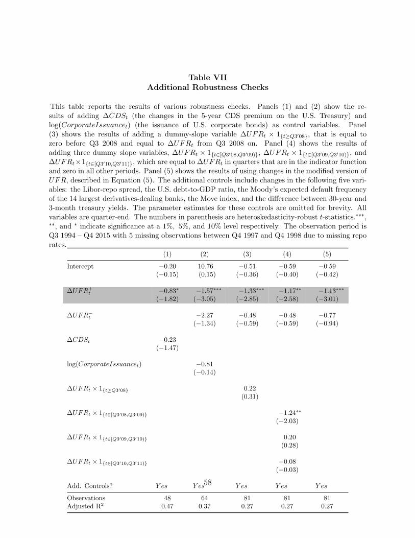
Table VIIAdditional Robustness Checks

This table reports the results of various robustness checks. Panels (1) and (2) show the re-sults of adding �CDSt (the changes in the 5-year CDS premium on the U.S. Treasury) andlog(CorporateIssuancet) (the issuance of U.S. corporate bonds) as control variables. Panel(3) shows the results of adding a dummy-slope variable �UFRt ⇥ 1{t�Q3008}, that is equal tozero before Q3 2008 and equal to �UFRt from Q3 2008 on. Panel (4) shows the results ofadding three dummy slope variables, �UFRt ⇥ 1{t2[Q3008,Q3009)}, �UFRt ⇥ 1{t2[Q3009,Q3010)}, and�UFRt⇥1{t2[Q3010,Q3011)}, which are equal to �UFRt in quarters that are in the indicator functionand zero in all other periods. Panel (5) shows the results of using changes in the modified version ofUFR, described in Equation (5). The additional controls include changes in the following five vari-ables: the Libor-repo spread, the U.S. debt-to-GDP ratio, the Moody’s expected default frequencyof the 14 largest derivatives-dealing banks, the Move index, and the di↵erence between 30-year and3-month treasury yields. The parameter estimates for these controls are omitted for brevity. Allvariables are quarter-end. The numbers in parenthesis are heteroskedasticity-robust t-statistics.⇤⇤⇤,⇤⇤, and ⇤ indicate significance at a 1%, 5%, and 10% level respectively. The observation period isQ3 1994 – Q4 2015 with 5 missing observations between Q4 1997 and Q4 1998 due to missing reporates.

(1) (2) (3) (4) (5)

Intercept �0.20 10.76 �0.51 �0.59 �0.59(�0.15) (0.15) (�0.36) (�0.40) (�0.42)

�UFR

+t �0.83⇤ �1.57⇤⇤⇤ �1.33⇤⇤⇤ �1.17⇤⇤ �1.13⇤⇤⇤

(�1.82) (�3.05) (�2.85) (�2.58) (�3.01)

�UFR

�t �2.27 �0.48 �0.48 �0.77

(�1.34) (�0.59) (�0.59) (�0.94)

�CDSt �0.23(�1.47)

log(CorporateIssuancet) �0.81(�0.14)

�UFRt ⇥ 1{t�Q3008} 0.22(0.31)

�UFRt ⇥ 1{t2[Q3008,Q3009)} �1.24⇤⇤

(�2.03)

�UFRt ⇥ 1{t2[Q3009,Q3010)} 0.20(0.28)

�UFRt ⇥ 1{t2[Q3010,Q3011)} �0.08(�0.03)

Add. Controls? Y es Y es Y es Y es Y es

Observations 48 64 81 81 81Adjusted R2 0.47 0.37 0.27 0.27 0.27

58

Table VIIISummary Statistics for International Data

This table shows summary statistics of pension fund underfunding and 30-year swap spreads forJapan and the Netherlands. UFR

Japt is constructed based on Equation (6). 30-yr SS (Jap) is the

di↵erence between the fixed rate in a 30-year IRS where the fixed rate is exchanged against 6-monthJapanese Libor rates and the bond yield of the most recently issued Japanese government bondwith 30-years to maturity. UFR

Netht is constructed based on Equation (7). 30-yr SS (Ger) and

30-yr SS (Neth) are the di↵erence between the fixed rate in a 30-year IRS where the fixed rate isexchanged against annual Euribor rates and the bond yield of the most recently issued German orDutch government bond with 30-years to maturity, respectively. The sample period in Panel A isQ1 2005 – Q4 2015. The sample period in Panel B is Q1 2007 – Q4 2014. # Under counts thenumber of quarters where pension funds are underfunded.

Mean SD Min Median Max # Obs # Under

Panel A: Summary statistics for Japan

UFR

Japt 28.88 7.25 17.38 28.04 41.17 44 44

30-yr SS (Jap) -0.11 11.73 -24.94 -0.65 26.34 44 �

Panel B: Summary statistics for the Netherlands

UFR

Netht -8.83 11.81 -34.14 -7.38 8.99 32 12

30-yr SS (Ger) 0.16 12.31 -25.85 2.04 23.10 32 �30-yr SS (Neth) -11.83 15.32 -47.55 -14.42 16.00 32 �

59

Table IXPension Fund Underfunding and Swap Spreads in Other Regions

This table reports results from regressions of quarterly changes in swap spreads with 2, 5, 10, and 30 yearsto maturity on the indicated variables. In Panel A, the swap spreads are computed as the di↵erence betweenthe fixed rate in an IRS based on Japanese Libor rates and Japanese government bond yields. �UFR

+t is

the change in the underfunding ratio of Japanese pension funds as defined in Equation (6), conditional onpension funds being underfunded at time t. There are no time periods where Japanese pension funds arefully funded. �LR Spreadt is the change in the quarter-end di↵erence between the 6-month Japanese Liborrate and 6-month General Collateral repo rate. In Panel B, the swap spreads are computed as the di↵erencebetween the fixed rate in an IRS based on Euribor and German government bond yields. Under 30 Year(Neth), the swap spread is computed relative to the Dutch government bond yield. �UFR

+t (�UFR

�t )

is the change in the underfunding ratio of Dutch pension funds as defined in Equation (7), conditional onpension funds being underfunded (funded) at time t. Pension funds are underfunded if the policy fundingratio drops below 105%. The numbers in parenthesis are heteroskedasticity-robust t-statistics. ⇤⇤⇤, ⇤⇤, and ⇤

indicate significance at a 1%, 5%, and 10% level respectively. The observation period is Q1 2005 – Q4 2015for Japan and Q1 2007 – Q4 2014 for the Netherlands.

Panel A: Regression analysis for Japan

2 Year 5 Year 10 Year 30 Year

Intercept �0.05 0.00 �0.20 �1.06(�0.08) (0.00) (�0.28) (�0.84)

�UFR

+t �0.28 �0.28 �1.00⇤⇤⇤ �2.02⇤⇤⇤

(�1.18) (�1.02) (�3.72) (�4.45)

�LR Spreadt 0.23⇤⇤⇤ 0.12 �0.05 0.06(3.04) (1.01) (�0.39) (0.38)

Observations 43 43 43 43Adjusted R2 0.11 0.00 0.32 0.34

Panel B: Regression analysis for the Netherlands

2 Year 5 Year 10 Year 30 Year 30 Year (Neth)

Intercept 0.98 0.72 �0.29 �0.90 �0.52(0.30) (0.23) (�0.14) (�0.59) (�0.25)

�UFR

+t 1.92⇤ 1.65 0.89 �1.27⇤⇤⇤ �1.11⇤⇤

(1.85) (1.49) (1.28) (�4.29) (�2.31)

�UFR

�t 0.25 0.57 0.76⇤⇤ �0.09 �0.43

(0.27) (1.15) (2.42) (�0.32) (�1.17)

Observations 31 31 31 31 31Adjusted R2 0.05 0.06 0.13 0.16 0.09

60

Previous volumes in this series

No Title Author

704 February 2018

Are credit rating agencies discredited? Measuring market price effects from agency sovereign debt announcements

Mahir Binici, Michael Hutchison and Evan Weicheng Miao

703 February 2018

The negative interest rate policy and the yield curve

Jing Cynthia Wu and Fan Dora Xia

702 February 2018

Cross-stock market spillovers through variance risk premiums and equity flows

Masazumi Hattori , Ilhyock Shim and Yoshihiko Sugihara

701 February 2018

Mapping shadow banking in China: structure and dynamics

Torsten Ehlers, Steven Kong and Feng Zhu

700 February 2018

The perils of approximating fixed-horizon inflation forecasts with fixed-event forecasts

James Yetman

699 February 2018

Deflation expectations Ryan Banerjee and Aaron Mehrotra

698 February 2018

Money and trust: lessons from the 1620s for money in the digital age

Isabel Schnabel and Hyun Song Shin

697 February 2018

Are banks opaque? Evidence from insider trading

Fabrizio Spargoli and Christian Upper

696 January 2018

Monetary policy spillovers, global commodity prices and cooperation

Andrew Filardo, Marco Lombardi, Carlos Montoro and Massimo Ferrari

695 January 2018

The dollar exchange rate as a global risk factor: evidence from investment

Stefan Avdjiev, Valentina Bruno, Catherine Koch and Hyun Song Shin

694 January 2018

Exchange Rates and the Working Capital Channel of Trade Fluctuations

Valentina Bruno, Se-Jik Kim and Hyun Song Shin

693 January 2018

Family first? Nepotism and corporate investment

Gianpaolo Parise, Fabrizio Leone and Carlo Sommavilla

692 January 2018

Central Bank Forward Guidance and the Signal Value of Market Prices

Stephen Morris and Hyun Song Shin

691 January 2018

Effectiveness of unconventional monetary policies in a low interest rate environment

Andrew Filardo and Jouchi Nakajima

All volumes are available on our website www.bis.org.