bird mortality from the deepwater horizon oil spill. i ... · pdf filebird mortality from the...

The following supplement accompanies the article

Bird mortality from the Deepwater Horizon oil spill. I. Exposure probability in the offshore Gulf of Mexico

J. Christopher Haney1,4,*, Harold J. Geiger2, Jeffrey W. Short3

1Terra Mar Applied Sciences LLC, 123 W. Nye Lane, Suite 129, Carson City, NV 89706, USA 2St. Hubert Research Group, 222 Seward, Suite 205, Juneau, AK 99801, USA

3JWS Consulting LLC, 19315 Glacier Highway, Juneau, AK 99801, USA 4Present address: Defenders of Wildlife, 1130 17th Street, NW, Washington DC 20036, USA

*Corresponding author: [email protected]

Marine Ecology Progress Series 513: 225–237 (2014)

Supplement. Origins of the spatial parameters used to estimate bird mortality in the offshore Gulf of Mexico during the 2010 Deepwater Horizon blowout, including daily oil slick size, other measures of surface spill extent, and seabird movements and replacement rates

Data sources for surface oil

Delineation of the extent of surface oil during the Deepwater Horizon blowout was primarily based on the Experimental Marine Pollution Surveillance Daily Composite Product (hereafter ‘Product’; Fig. S1). These were experimental syntheses developed by the Satellite Analysis Branch, National Oceanic and Atmospheric Administration, for identifying surface oil anomalies associated with the Deepwater Horizon blowout.

Products were compiled by analysts who relied on satellite imagery and supplemental data (e.g. Good et al. 2011) to map the locations and minimal extent of Deepwater Horizon surface oil. Over 300 of these Products were created and are accessible publicly at www.ssd.noaa.gov/PS/MPS/deepwater.html (accessed 6 August 2013).

Fig. S1. Satellite-derived composite of the estimated surface area of oil from the Deepwater Horizon blowout on 19 June 2010

Oil surface area measurement Generation of the Products and accompanying image analyses were performed in

an ArcGIS (Streett 2011). Ancillary data such as natural oil seeps, oil platforms, surface winds, and so on were imported as part of this GIS. To estimate daily extent of surface oil beyond 40 km of the Gulf coastline, we excised and measured this offshore portion of the Product shape file for oil using a GIS (Fig. S2).

Analysts generally incorporated spatially explicit information that had been obtained from multiple satellite passes and/or imagery collected by different satellite sensors each day to generate the Product. Spatial resolution of sensing platforms could vary by an order of magnitude (Table S1), so that the spatial extent covered by individual images could be smaller than the total surface extent of Deepwater Horizon oil on any given day.

Fig. S2. Shape file for estimated oil extent on 19 June 2010 (cf. Fig. S1), illustrating how oil surface area >40 km from the Gulf coastline (black) was excised with a GIS (green line) to distinguish it from the extent

of oil surface area <40 km from the coastline (yellow)

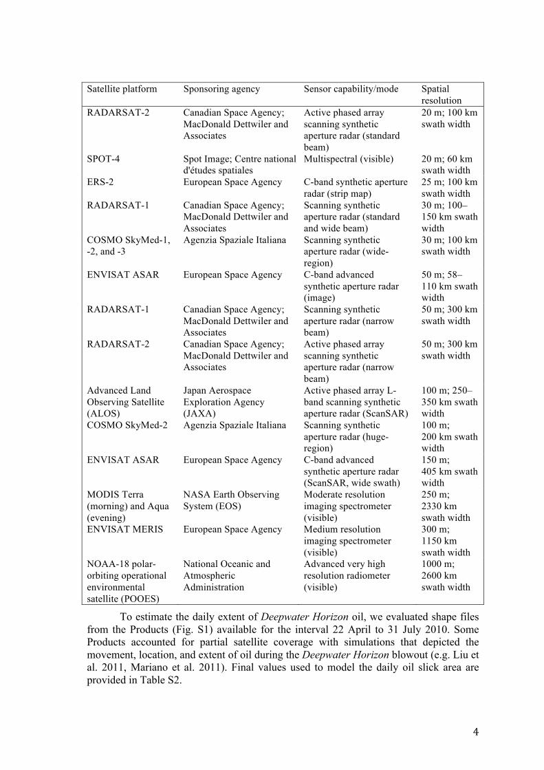
Table S1. Orbiting remote sensors used to delineate the extent of surface oil during the Deepwater Horizon blowout. Sensors are listed in decreasing order of spatial resolution, and increasing swath width or image

scene size

Satellite platform Sponsoring agency Sensor capability/mode Spatial resolution

TerraSAR-X Deutsches Zentrum für Luft- und Raumfahrt

Active phased array scanning synthetic aperture radar (SpotLight)

1 m; 5–10 km swath width


Active phased array scanning synthetic aperture radar (StripMap)


RADARSAT-2 Canadian Space Agency; MacDonald Dettwiler and Associates

Active phased array scanning synthetic aperture radar (fine beam)

8 m; 50 km swath width

ASTER NASA/Jet Propulsion Laboratory

Multispectral (very near infrared)


LANDSAT-7 NASA, United States Geological Survey

Enhanced thematic mapper

15–80 m; 185 km swath width


Active phased array scanning synthetic aperture radar (ScanSAR)


Satellite platform Sponsoring agency Sensor capability/mode Spatial resolution


Active phased array scanning synthetic aperture radar (standard beam)


SPOT-4 Spot Image; Centre national d'études spatiales

Multispectral (visible) 20 m; 60 km swath width

ERS-2 European Space Agency C-band synthetic aperture radar (strip map)



Scanning synthetic aperture radar (standard and wide beam)


COSMO SkyMed-1, -2, and -3

Agenzia Spaziale Italiana Scanning synthetic aperture radar (wide-region)


ENVISAT ASAR European Space Agency C-band advanced synthetic aperture radar (image)



Scanning synthetic aperture radar (narrow beam)



Active phased array scanning synthetic aperture radar (narrow beam)


Advanced Land Observing Satellite (ALOS)

Japan Aerospace Exploration Agency (JAXA)

Active phased array L-band scanning synthetic aperture radar (ScanSAR)


COSMO SkyMed-2 Agenzia Spaziale Italiana Scanning synthetic aperture radar (huge-region)


ENVISAT ASAR European Space Agency C-band advanced synthetic aperture radar (ScanSAR, wide swath)


MODIS Terra (morning) and Aqua (evening)

NASA Earth Observing System (EOS)

Moderate resolution imaging spectrometer (visible)


ENVISAT MERIS European Space Agency Medium resolution imaging spectrometer (visible)


NOAA-18 polar-orbiting operational environmental satellite (POOES)

National Oceanic and Atmospheric Administration

Advanced very high resolution radiometer (visible)


To estimate the daily extent of Deepwater Horizon oil, we evaluated shape files from the Products (Fig. S1) available for the interval 22 April to 31 July 2010. Some Products accounted for partial satellite coverage with simulations that depicted the movement, location, and extent of oil during the Deepwater Horizon blowout (e.g. Liu et al. 2011, Mariano et al. 2011). Final values used to model the daily oil slick area are provided in Table S2.

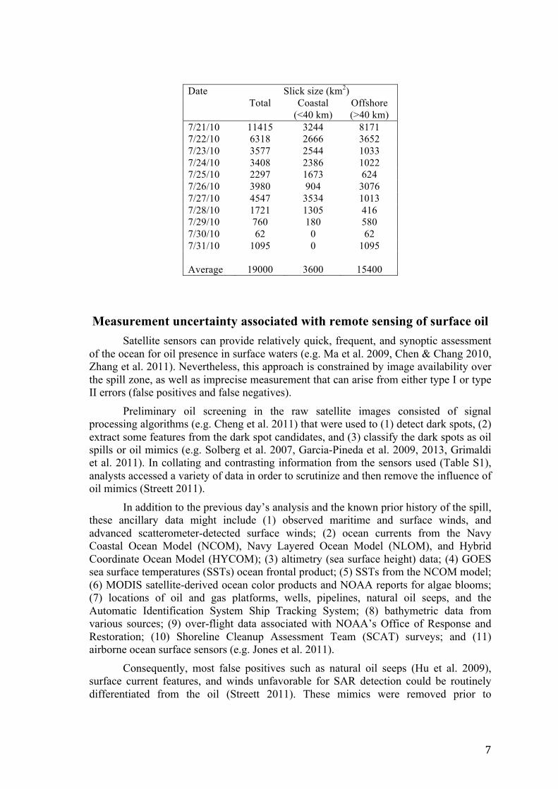
Table S2. Daily estimates of oil slick area (in km2) during the Deepwater Horizon blowout including area estimates in coastal (<40 km) and in offshore (>40 km) waters of the spill zone in the northern Gulf of

Mexico (see also Fig. S2). More than 80% of the cumulative oil slick area (km2-days) occurred ≥40 km offshore

Date Slick size (km2) Total Coastal

(<40 km) Offshore (>40 km)

4/20/10 0 0 0 4/21/10 0 0 0 4/22/10 62 0 62 4/23/10 1095 0 1095 4/24/10 1992 0 1992 4/25/10 4201 0 4201 4/26/10 N/A N/A N/A 4/27/10 N/A N/A N/A 4/28/10 N/A N/A N/A 4/29/10 N/A N/A N/A 4/30/10 4750 600 4150 5/1/10 N/A N/A N/A 5/2/10 N/A N/A N/A 5/3/10 15716 5158 10558 5/4/10 12472 1670 10802 5/5/10 N/A N/A N/A 5/6/10 5413 345 5068 5/7/10 10591 2333 8258 5/8/10 19929 899 19030 5/9/10 25860 1072 24788 5/10/10 20393 915 19478 5/11/10 31547 529 31018 5/12/10 23926 2223 21703 5/13/10 51588 9617 41971 5/14/10 19360 9288 10072 5/15/10 29979 7867 22112 5/16/10 50507 4044 46463 5/17/10 73462 14872 58590 5/18/10 35987 8140 27847 5/19/10 21467 5049 16418 5/20/10 21911 3638 18273 5/21/10 28106 6806 21300 5/22/10 50236 20849 29387 5/23/10 31559 7624 23935 5/24/10 N/A N/A N/A 5/25/10 40815 9507 31308 5/26/10 18331 2808 15523 5/27/10 37644 4831 32813 5/28/10 35787 2637 33150 5/29/10 31057 2064 28993 5/30/10 41037 5757 35280 5/31/10 16871 1726 15145 6/1/10 28074 3256 24818



6/2/10 3216 1629 1587 6/3/10 5484 437 5047 6/4/10 9907 959 8948 6/5/10 14551 754 13797 6/6/10 40240 4851 35389 6/7/10 9927 553 9374 6/8/10 25082 3509 21573 6/9/10 17856 3083 14773 6/10/10 27384 4503 22881 6/11/10 28771 4335 24436 6/12/10 24746 3758 20988 6/13/10 49612 7674 41938 6/14/10 32763 6055 26708 6/15/10 30273 3537 26736 6/16/10 22858 1428 21430 6/17/10 82648 3457 79191 6/18/10 28295 1132 27163 6/19/10 27769 1274 26495 6/20/10 35175 3321 31854 6/21/10 53949 13774 40175 6/22/10 12708 2942 9766 6/23/10 31003 9119 21884 6/24/10 43324 11361 31963 6/25/10 40809 15460 25349 6/26/10 18632 9624 9008 6/27/10 19554 9699 9855 6/28/10 8151 3785 4366 6/29/10 6062 4488 1574 6/30/10 24780 11349 13431 7/1/10 6829 3492 3337 7/2/10 4279 1272 3007 7/3/10 6344 1993 4351 7/4/10 11051 2619 8432 7/5/10 7646 1843 5803 7/6/10 7922 2523 5399 7/7/10 11361 5071 6290 7/8/10 6722 1351 5371 7/9/10 8497 1051 7446 7/10/10 4119 200 3919 7/11/10 4205 69 4136 7/12/10 10629 103 10526 7/13/10 6849 72 6777 7/14/10 6370 73 6297 7/15/10 6999 319 6680 7/16/10 8052 762 7290 7/17/10 20764 2403 18361 7/18/10 9225 1586 7639 7/19/10 5074 1688 3386 7/20/10 376 344 32



7/21/10 11415 3244 8171 7/22/10 6318 2666 3652 7/23/10 3577 2544 1033 7/24/10 3408 2386 1022 7/25/10 2297 1673 624 7/26/10 3980 904 3076 7/27/10 4547 3534 1013 7/28/10 1721 1305 416 7/29/10 760 180 580 7/30/10 62 0 62 7/31/10 1095 0 1095 Average 19000 3600 15400

Measurement uncertainty associated with remote sensing of surface oil Satellite sensors can provide relatively quick, frequent, and synoptic assessment

of the ocean for oil presence in surface waters (e.g. Ma et al. 2009, Chen & Chang 2010, Zhang et al. 2011). Nevertheless, this approach is constrained by image availability over the spill zone, as well as imprecise measurement that can arise from either type I or type II errors (false positives and false negatives).

Preliminary oil screening in the raw satellite images consisted of signal processing algorithms (e.g. Cheng et al. 2011) that were used to (1) detect dark spots, (2) extract some features from the dark spot candidates, and (3) classify the dark spots as oil spills or oil mimics (e.g. Solberg et al. 2007, Garcia-Pineda et al. 2009, 2013, Grimaldi et al. 2011). In collating and contrasting information from the sensors used (Table S1), analysts accessed a variety of data in order to scrutinize and then remove the influence of oil mimics (Streett 2011).

In addition to the previous day’s analysis and the known prior history of the spill, these ancillary data might include (1) observed maritime and surface winds, and advanced scatterometer-detected surface winds; (2) ocean currents from the Navy Coastal Ocean Model (NCOM), Navy Layered Ocean Model (NLOM), and Hybrid Coordinate Ocean Model (HYCOM); (3) altimetry (sea surface height) data; (4) GOES sea surface temperatures (SSTs) ocean frontal product; (5) SSTs from the NCOM model; (6) MODIS satellite-derived ocean color products and NOAA reports for algae blooms; (7) locations of oil and gas platforms, wells, pipelines, natural oil seeps, and the Automatic Identification System Ship Tracking System; (8) bathymetric data from various sources; (9) over-flight data associated with NOAA’s Office of Response and Restoration; (10) Shoreline Cleanup Assessment Team (SCAT) surveys; and (11) airborne ocean surface sensors (e.g. Jones et al. 2011).

Consequently, most false positives such as natural oil seeps (Hu et al. 2009), surface current features, and winds unfavorable for SAR detection could be routinely differentiated from the oil (Streett 2011). These mimics were removed prior to

generating the Product estimates for surface oil extent during Deepwater Horizon. One notable exception was the floating macroalga Sargassum. Separating Sargassum from oil was difficult in late July and August when small patches of presumed oil were no longer contiguous with the spill’s origin (Streett 2011). Moreover, due to physical aggregation by surface current features in the Gulf, patches of Sargassum and Deepwater Horizon oil could be found together in the same debris fields (e.g. Carmichael et al. 2012).

In contrast to modest uncertainty from over-estimating oil extent due to image pixel exaggeration (Hu et al. 2009) or oil mimicry, the variety and prevalence of false negatives were more difficult to mitigate. Factors that led to under-estimating oil extent in satellite images during Deepwater Horizon included (1) limitations of sensor pass coverage (incomplete imagery, or imagery cut-off); (2) only lower-resolution imagery available on some days, thereby missing smaller oil patches; (3) image obstruction of oil by clouds, rain, and convection; (4) inability to detect oil with synthetic aperture radar (SAR) when winds were chaotic, or when winds (if consistent) were below (or above) the optimal detection range for this sensor; (5) shadowing in the SAR imagery due to the coastline, bathymetry, and currents; (6) low detection as a consequence of SAR incident angle and beam mode (Garcia-Pineda et al. 2013), and (7) indistinct boundaries or undetected oil due to unfavorable sun-glint angle in images from the Moderate Resolution Imaging Spectroradiometer (MODIS).

Furthermore, satellite sensors cannot detect oil thicknesses or patch sizes below certain thresholds (Fingas & Brown 1997, Brekke & Solberg 2005). Thus, smaller oil patches, thin oil sheens, and dissolved hydrocarbons (e.g. Liu et al. 2014) can go undetected altogether. Along with satellite passes that missed the Deepwater Horizon spill zone, and image cutoffs when the coverage was only partial, the overall uncertainty associated with under-estimation of oil extent is likely to have been substantial. We thus consider measurements of the daily slick size and cumulative spill area rendered by syntheses in the Daily Composite Products (Fig. S1) presented here (Table S2) to represent minimal estimates for the spatial extent of oil during the Deepwater Horizon blowout.

The various data corrections noted above when applied to estimation of daily slick size addressed only the relative (not absolute) limitations in the satellite coverage across the spill zone. Therefore, gaps caused by missing data would in the aggregate tend to under-estimate the exposure risk to marine birds in the Gulf of Mexico during the Deepwater Horizon discharge.

Migration and replacement of seabirds over the oil spill zone The exposure period duration P required for replenishment of birds killed by oil

exposure is assumed to be determined by some combination of the movement of the oil slick relative to birds, movement of local birds relative to the oil slick, and regional bird influx due to exogenous migration (Fig. S3). Maximum distances across the Deepwater Horizon’s cumulative oiled area were approximately 500 to 550 km. At flight speeds of 15 to 45 km h–1 (e.g. Spear et al. 2004), it would take the slowest marine birds less than a day to reach the oil slick’s interior from adjacent unpolluted waters if they flew directly toward the center of the slick, with random flight taking somewhat longer.

Theoretically, local repopulation would be feasible within a day or so for the oiled zone, including the entire offshore portion. Assuming a mortality process that removed a third of all birds present over the slick, local movement rates from outside the spill zone need not be especially high to maintain bird density over time (see Fifield et al. 2009). More importantly, seasonal migrations could maintain bird density throughout the total oil exposure period, as more than 75% of offshore birds in the Gulf of Mexico breed outside the region entirely, with some species immigrating from very long distances into the Gulf throughout the duration of the spill (Fig. S3; see also Peake 1996).

Leach’s Storm-Petrel

Band-rumped Storm-Petrel

Great Shearwater

Masked Booby

(see inset)

inset

Leach’

mped

Shearwater

assskkked BooBBk byyyy

Fig. S3. Nearest breeding origins of some Atlantic seabirds known to have been killed (solid line) or vul-nerable to being killed (dashed line) by the Deepwater Horizon blowout. Masked booby Sula dactylatra, Leach’s storm-petrel Oceanodroma leucorhoa, and great shearwater Puffinus gravis mortalities are doc-umented in the official spill database (www.fws.gov/home/dhoilspill/collectionreports.html; accessed 22 Feb 2013). Origin and presence of band-rumped storm-petrel Oceanodroma castro in the Gulf of Mexico

are based on banding recovery (Woolfenden et al. 2001)

As the spill began, winter residents were departing the spill zone (e.g. northern gannet Morus bassanus; Montevecchi et al. 2012). However, eastern Atlantic species such as band-rumped storm-petrel Oceanodroma castro arrive during May-July via long distance migration (Stotterback 2002). Fall migrants (e.g. black tern Chlidonias niger, jaegers Stercorarius spp.) return south to the spill zone during July–August (Ribic et al. 1997, Heath et al. 2009). Offshore bird abundance was further augmented by nonbreeding and post-breeding Audubon’s shearwater Puffinus lherminieri, masked booby Sula dactylatra, and bridled tern Onychoprion anaethetus, all of which disperse into the spill zone from further south and east during summer months (e.g. Ribic et al. 1997).

Large-scale movements of seabirds are strongly affected by wind direction (Adams & Flora 2010). During the 103 d period of the Deepwater Horizon blowout, offshore wind direction changed by 60° or more 21 times, on average about every 5 d (see Supplement for Haney et al. 2014, available at www.int-res.com/articles/suppl/ m513p227_supp.pdf). Based on the factors noted above, we therefore estimated time to restore density to the initial level of D following the loss of birds due to mortality to be every 4 d, on average, with uncertainty in P assessed by assigning this parameter a uniform distribution on the interval 2 to 6 d.

LITERATURE CITED

Adams J, Flora S (2010) Correlating seabird movements with ocean wind: linking satellite telemetry with ocean scatterometry. Mar Biol 157:915–929

Brekke C, Solberg AHS (2005) Oil spill detection by satellite remote sensing. Remote Sens Environ 95:1–13

Carmichael CA, Arey JS, Graham WM, Linn LJ, Lemkau KL, Nelson RK, Reddy CM (2012) Floating oil-covered debris from Deepwater Horizon: identification and application. Environ Res Lett 7:015301

Chen CF, Chang LY (2010) Extraction of oil slicks on the sea surface from optimal satellite images by using an anomaly detection technique. J Appl Remote Sens 4:043565

Cheng Y, Li X, Xu Q, Garcia-Pineda O, Andersen OB, Pichel WG (2011) SAR observation and model tracking of an oil spill event in coastal waters. Mar Pollut Bull 62:350–363

Fifield DA, Baker KD, Byrne R, Robertson GJ and others (2009) Modelling seabird oil spill mortality using flight and swim behaviour. Environ Stud Res Fund Rep 186, Canadian Wildlife Service, Dartmouth, NS

Fingas MF, Brown CE (1997) Review of oil spill remote sensing. Spill Sci Technol Bull 4:199–208

Garcia-Pineda O, Zimmer B, Howard M, Pichel W, Li X, MacDonald IR (2009) Using SAR images to delineate ocean oil slicks with a texture classifying neural network algorithm (TCNNA). Can J Remote Sens 35:411–421

Garcia-Pineda O, MacDonald I, Hu C, Svejkovsky J, Hess M, Dukhovskoy D, Morey SL (2013) Detection of floating oil anomalies from the Deepwater Horizon oil spill with synthetic aperture radar. Oceanography 26:124–137

Good WS, Warden R, Kaptchen PF, Finch T, Emery WJ, Giacomini A (2011) Absolute airborne thermal SST measurements and satellite data analysis from the Deepwater Horizon oil spill. In: Liu Y, MacFadyen A, Ji ZG, Weisberg RH (eds) Monitoring and modeling the Deepwater Horizon oil spill: a record-breaking enterprise. Geophys Monogr Ser 195. American Geophysical Union, Washington DC, p 51–61

Grimaldi CSL, Coviello I, Lacava T, Pergola N, Tramutoli V (2011) A new RST-based approach for continuous oil spill detection in TIR range: the case of the Deepwater Horizon platform in the Gulf of Mexico. In: Liu Y, MacFadyen A, Ji ZG, Weisberg RH (eds) Monitoring and modeling the Deepwater Horizon oil spill: a record-

breaking enterprise. Geophys Monogr Ser 195. American Geophysical Union, Washington DC, p 19–31

Haney JC, Geiger HJ, Short JW (2014) Bird mortality from the Deepwater Horizon oil spill. II. Carcass sampling and exposure probability in the coastal Gulf of Mexico. Mar Ecol Prog Ser 512:227–240

Heath SR, Dunn EH, Agro DJ (2009) Black tern (Chlidonias niger). In: Poole A (ed) The birds of North America online. Cornell Lab of Ornithology, Ithaca, NY http://bna.birds.cornell.edu/bna/species/147 (accessed 26 Feb 2013)

Hu C, Li X, Pichel WG, Muller-Karger FE (2009) Detection of natural oil slicks in the NW Gulf of Mexico using MODIS imagery. Geophys Res Lett 36:L01604, doi:10.1029/2008GL036119

Jones CE, Minchew B, Holt B, Hensley S (2011) Studies of the Deepwater Horizon oil spill with the UAVSAR radar. In: Liu Y, MacFadyen A, Ji ZG, Weisberg RH (eds) Monitoring and modeling the Deepwater Horizon oil spill: a record-breaking enterprise. Geophys Monogr Ser 195. American Geophysical Union, Washington DC, p 33–50

Liu Y, Weisberg RH, Hu C, Zheng L (2011) Trajectory forecast as a rapid response to the Deepwater Horizon oil spill. In: Liu Y, MacFadyen A, Ji ZG, Weisberg RH (eds) Monitoring and modeling the Deepwater Horizon oil spill: a record-breaking enterprise. Geophys Monogr Ser 195. American Geophysical Union, Washington DC, p 153–165

Liu Z, Liu J, Gardner WS, Shank GC, Nathaniel EO (2014) The impact of Deepwater Horizon oil spill on petroleum hydrocarbons in surface waters of the northern Gulf of Mexico Deep-Sea Res II (in press) doi:10.1016/j.dsr2.2014.01.013

Ma L, Li Y, Liu Y (2009) Oil spill monitoring based on its spectral characteristics. Environ Forensics 10:317–323

Mariano AJ, Kourafalou VH, Srinivasan A, Kang H, Halliwell GR, Ryan EH, Roffer M (2011) On the modeling of the 2010 Gulf of Mexico oil spill. Dyn Atmos Oceans 52:322–340

Montevecchi W, Fifield D, Burke C, Garthe S, Hedd A, Rail JF, Robertson G (2012) Tracking long-distance migration to assess marine pollution impact. Biol Lett 8: 218–221

Peake DE (1996) Bird surveys. In: Davis RW, Fargion GS (eds) Distribution and abundance of cetaceans in the north-central and western Gulf of Mexico. Volume II Tech Rep, OCS Study MMS 96-0027. US Dept Interior, New Orleans, LA, p 271–304

Ribic CA, Davis R, Hess N, Peake D (1997) Distribution of seabirds in the northern Gulf of Mexico in relation to mesoscale features: initial observations. ICES J Mar Sci 54:545–555

Solberg AHS, Brekke C, Ove Husoy P (2007) Oil spill detection in RADARSAT and EINVISAT SAR images. IEEE Trans Geosci Rem Sens 45:746–755

Spear LB, Ainley DG, Hardesty BD, Howell SNG, Webb SW (2004) Reducing biases affecting at-sea surveys of seabirds: use of multiple observer teams. Mar Ornithol 32:147–157

Stotterback J (2002) Band-rumped storm-petrel (Oceanodroma castro). In: Poole A (ed) The birds of North America online. Cornell Lab of Ornithology, Ithaca, NY http://bna.birds.cornell.edu/bna/species/673a (accessed 26 Feb 2013)

Streett D (2011) NOAA's satellite monitoring of marine oil. In: Liu Y, MacFadyen A, Ji ZG, Weisberg RH (eds) Monitoring and modeling the Deepwater Horizon oil spill: a record-breaking enterprise. Geophys Monogr Ser 195. American Geophysical Union, Washington DC, p 9–18

Woolfenden GE, Monteiro LR, Duncan RA (2001) Recovery from the northeastern Gulf of Mexico of a band-rumped storm-petrel banded in the Azores. J Field Ornithol 72:62–65

Zhang B, Perrie W, Li X, Pichel WG (2011) Mapping seas surface oil slicks using RADARSAT-2 quad-polarization SAR image. Geophys Res Lett 38:L10602, doi:10.1029/2011GL047013

bird mortality from the deepwater horizon oil spill. i ... · pdf filebird mortality from the...

Documents