1

Biospeckle-based Studyof the Line Profile of

Light Scattered in Strawberries

Master Thesisby

Anders Bergkvist

Lund Reports on Atomic Physics, LRAP-220Lund 1997

This thesis was carried out atCentro de Investigaciones Opticas (CIOp) in La Plata, Argentina,

and submitted to theFaculty of Technology at Lund University

in partial fulfilment of the requirements for the degree ofMaster of Science

2

Abstract

The line profiles of light scattered in strawberries were measured with a biospeckleapproach. This method allows studies of extremely small shifts (0.1 Hz) in matterconsisting of randomly moving particles. The method is independent of the numberand types of particles in the object. 512 timehistories of different areas in the specklepattern were simultaneously recorded. The timehistories were autocorrelated andFourier transformed to obtain the frequency spectra of the scattered light. This lineprofile was compared with a Voight profile to determine the ratio of Lorentzian toGaussian line shape in it. It was found that Lorentzian line profile originates fromdiffusive movements in the object and the Gaussian from turbulent movements as wellas from speed of particles in the object. The changes in diffusive activity correlateswith changes in the cell wall structure, and the changes in Gaussian line widthcorrelates with the flow of particles into the vacoules of the cells.

3

Table of contents

1. Introduction…………………………………………………………… 3

1.1. Background…………………………………………………………. 3

1.2. Objectives…………………………………………………………… 4

1.3. Limitations………………………………………………………….. 4

2. Theoretical Aspects………………………………………………….. 5

2.1. Light interaction with biological tissue…………………………… 5

2.1.1. Light-matter interaction……………………………………….. 52.1.2. Composition and structure of biological tissue……………….. 82.1.3. Optical properties of biological tissue………………………… 9

2.2. Speckles …………………………………………………………….. 13

2.2.1. Laser speckles.............................………………………………132.2.2. Biospeckles..................................……………………………..142.2.3. Properties of biospeckles……………………………………… 15

2.3. Autocorrelation and the Wiener-Khinchin theorem…………….. 18

2.4. The line profile and its origin …………………………………….. 23

2.4.1. The Doppler effect…………………………………………….. 232.4.2. Turbulence.............................………………………………….242.4.3. Diffusion.............................……………………………………242.4.4. The Voight profile.............................………………………….252.4.5. Other broadenings and shifts………………………………….. 28

2.5. The development of strawberries…………………………………. 29

3. Experimental study………………………………………………….. 33

3.1. Introduction………………………………………………………… 33

3.2. The experimental setup and equipment………………………….. 33

3.2.1. Setup A: With an expanded laser beam and without a diaphragm……………………………………… 333.2.2. Setup B: With a normal laser beam and with a diaphragm…………………………………………. 33

4

3.2.3. Equipment…………………………………………………….. 353.2.4. Computer programs …………………………………………… 35

3.3. Experimental procedure…………………………………………… 36

3.4. Study of noise………………………………………………………. 37

3.4.1. Introduction…………………………………………………… 373.4.2. Results………………………………………………………… 37

3.5. Study of the line profile of light scatteredin different fruits and vegetables………………………………….. 40

3.5.1. Introduction…………………………………………………… 403.5.2. Results………………………………………………………… 40

3.6. Study of the line profile of light scatteredin strawberries during maturation ……………………………….. 42

3.6.1. Introduction…………………………………………………… 423.6.2. Results………………………………………………………… 42

4. Conclusion and Discussion………………………………………… 47

Acknowledgements …………………………………………………….. 49

List of references ……………………………………………………….. 51

Appendix A. Computer program FRUTY.C …………………….. 55

5

1. Introduction

1.1 Background

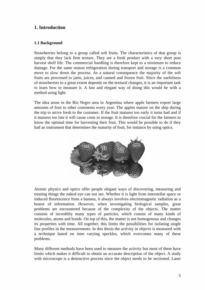
Strawberries belong to a group called soft fruits. The characteristics of that group issimply that they lack firm texture. They are a fresh product with a very short postharvest shelf life. The commercial handling is therefore kept to a minimum to reducedamage. For the same reason refrigeration during transport and storage is a commonmove to slow down the process. As a natural consequence the majority of the softfruits are processed to jams, juices, and canned and frozen fruit. Since the usefulnessof strawberries to a great extent depends on the textural changes, it is an important taskto learn how to measure it. A fast and elegant way of doing this would be with amethod using light.

The idea arose in the Rio Negro area in Argentina where apple farmers export largeamounts of fruit to other continents every year. The apples mature on the ship duringthe trip to arrive fresh to the customer. If the fruit matures too early it turns bad and ifit matures too late it will cause costs in storage. It is therefore crucial for the farmers toknow the optimal time for harvesting their fruit. This would be possible to do if theyhad an instrument that determines the maturity of fruit, for instance by using optics.

Atomic physics and optics offer people elegant ways of discovering, measuring andtreating things the naked eye can not see. Whether it is light from interstellar space orinduced fluorescence from a banana, it always involves electromagnetic radiation as abearer of information. However, when investigating biological samples, greatproblems are encountered because of the complexity of the objects. The matterconsists of incredibly many types of particles, which consist of many kinds ofmolecules, atoms and bonds. On top of this, the matter is not homogenous and changesits properties with time. All together, this limits the possibilities for isolating singleline profiles in the measurements. In this thesis the activity in objects is measured witha technique based on time varying speckles, which overcomes many of theseproblems.

Many different methods have been used to measure the activity but most of them havelimits which makes it difficult to obtain an accurate description of the object. A studywith microscope is a destructive process since the object needs to be sectioned. Laser

6

Doppler velocimetry measures the flow of particles in a certain direction andconsequently does not detect random movement. Laser spectroscopy is a remarkableinstrument for extracting information about a medium, but it is far too rough tomeasure the shifts caused by changes in the activity. The time varying speckleapproach however, can be used to do experiments independent of the number andtypes of particles in the object. This technique measures quality rather than quantity oflight and manages shifts within a few hertz.

The time varying speckle phenomenon has already been used to study a variety ofobjects that move in random ways. For example during the drying process of paint, themoving particles in it have been observed. The particles in the wet paint keep movinguntil the paint is completely dry [1]. The blood flow in superficial layers of skin hassuccessfully been studied in [2], the activity of micro-organisms in a solution in [3]and the decadence of fresh fruit in [4]. What they all have in common is that only theDoppler velocity of the particles in the matter is measured. Since the light scatteredfrom the object contains a lot more information about the processes in the matter, itought to be possible to extract it. This would lead to a possibility to solve the twoproblems concerning apples and strawberries.

1.2 Objectives

The objective of this thesis is to extract information from biospeckles about howchanges in cells influence light that is scattered inside the cells. The study is focusedon how the line profile of the scattered light changes with the activity in the fruits.Furthermore it is analysed if the scattered light can be described with the Voightprofile. Finally, as far as possible, the line profile is used to determine the maturity offruits.

1.3 Limitations

The statistical properties and mathematics for biospeckles have not yet beenestablished because of the complexity of the movements of living objects. I havetherefore an experimental approach to this study. Since the biological tissue is such acomplex medium, not only consisting of a large amount of different matters but is alsonon-homogeneous, it is necessary to do approximations to get an applicable model towork with. The matter is therefore regarded as homogeneous with a seedless surfaceand the internal activity independent of the depth in the tissue.

Because of the limited extent of this study it is not supplemented with simulationsabout the optical properties of fruit tissue. However, some of them have previouslybeen measured which gives an idea about the properties in the matters used in thiswork [4,5,6]. For the same reason the biospeckle experiments are not combined withother techniques (like for instance spectroscopy) to get a more complete representationof the objects.

7

2. Theoretical Aspects

2.1. Light interaction with biological tissue

2.1.1 Light-matter interaction

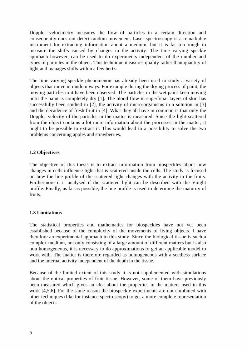
Light interacts with matter in various ways, figure 1. The different processes that occurdepend on the wavelength of the light as well as the structure of the medium. Light canbe reflected, scattered or absorbed when it interacts with the matter. Photons with veryhigh energy, like gamma and x-rays, may even ionise atoms or break bonds in themolecules, but this will not be the case in this work since visible light is being usedthrough all the experiments.

Figure 1. Various interactions between light and matter [7].

The reflection of the light, when it enters a border between different refractive indexes,obeys the laws of Snell and Fresnel. It depends therefore on the refractive indexes aswell as the angle of the incoming and the reflected rays:

n1 ⋅ sinϕ 1 = n2 ⋅sinϕ2 (Snell) (1)

R =1

2

sin2(ϕ1 − ϕ 2)

sin2(ϕ1 + ϕ 2)+

tan2(ϕ1 − ϕ2)

tan2(ϕ1 + ϕ2)

(Fresnel) (2)

n1, n2 are the refractive indexes in the two materials and ϕ1 , ϕ 2 the angles of the lightperpendicular to the boundary.

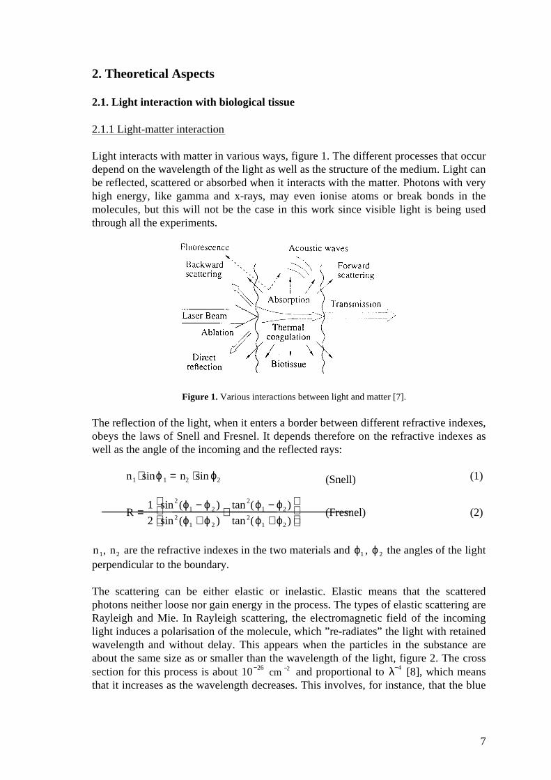
The scattering can be either elastic or inelastic. Elastic means that the scatteredphotons neither loose nor gain energy in the process. The types of elastic scattering areRayleigh and Mie. In Rayleigh scattering, the electromagnetic field of the incominglight induces a polarisation of the molecule, which ” re-radiates” the light with retainedwavelength and without delay. This appears when the particles in the substance areabout the same size as or smaller than the wavelength of the light, figure 2. The crosssection for this process is about 10−26 cm −2 and proportional to λ−4 [8], which meansthat it increases as the wavelength decreases. This involves, for instance, that the blue

8

light from the sun is scattered on the molecules in the air more than the red light, andtherefore makes the sky look blue.

������� ���� �� � ����� ν

����������� � � � �����! !"ν

#�$&%('*),+ ' )-+.�/103254

ν

687�9�: :�;=< ;> < 9�?A@

B ν

Figure 2. Rayleigh scattering on particles.

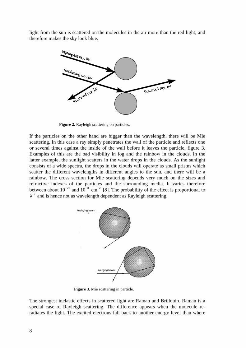
If the particles on the other hand are bigger than the wavelength, there will be Miescattering. In this case a ray simply penetrates the wall of the particle and reflects oneor several times against the inside of the wall before it leaves the particle, figure 3.Examples of this are the bad visibility in fog and the rainbow in the clouds. In thelatter example, the sunlight scatters in the water drops in the clouds. As the sunlightconsists of a wide spectra, the drops in the clouds will operate as small prisms whichscatter the different wavelengths in different angles to the sun, and there will be arainbow. The cross section for Mie scattering depends very much on the sizes andrefractive indexes of the particles and the surrounding media. It varies thereforebetween about 10−26 and 10−8 cm−2 [8]. The probability of the effect is proportional toλ−2 and is hence not as wavelength dependent as Rayleigh scattering.

Figure 3. Mie scattering in particle.

The strongest inelastic effects in scattered light are Raman and Brillouin. Raman is aspecial case of Rayleigh scattering. The difference appears when the molecule re-radiates the light. The excited electrons fall back to another energy level than where

9

they were before the polarisation, figure 4. This gives wavelengths shifted certainenergies, up or down, from the wavelength of the incoming light, specific for eachbond in the medium. Hydrogen has the largest shift and changes the energy 4155cm−1 , but the most common shifts are 100-1000 cm−1 [9]. The cross section for Ramanscattering is about 10−29

cm−2 .

C νD E νF

G H I J K L M M N O N M P

Q N L M M N O N M P

R S T U V W X Y Z [ V \ ] ^ _ ` S \ W S T U V W

Figure 4. Raman shifts of the scattered light [8].

Brillouin scattering appears when a crystal is deformed by a long acoustic phonon. Therefractive index of the crystal changes due to the tension that is induced by thevibration. Consequently, if a phonon is present it will affect the shifts and directions ofall the photons it encounters. The size of the changes, depends on the resonancefrequencies of the setup and hence the characteristics and size of the object, thelaboratory, the equipment and the phonon.

The absorption process is a very complex part of the interaction. The different atomsand molecules in the matter have a wide range of possible energy levels which can beexcited. After a certain time delay, also depending on the type of atoms or molecules,they loose energy by either producing heat, contributing to some photochemicalreaction or re-radiate photons in any direction, called fluorescence. These photons mayhave the same wavelengths as the incoming rays but also other, depending on theprobability for the occupation of the different energy levels. All this information isspecific for each medium and is therefore a good source when working withspectroscopy to extract information concerning the characteristics of the substance. Onthe other hand, since this study is depending on the correlation of the scattering indifferent media, the re-radiation may instead be a source of noise. The probabilities forabsorption and fluorescence are both normally about 10−16 cm−2 . However, in liquidsand solids at atmospheric pressure the molecules will be close enough to bounce in toeach other and stimulate the segregation of heat. This is called quenching and reducesthe probability of fluorescence to about 10−20 cm−2 [8].

10

2.1.2. Composition and structure of biological tissue

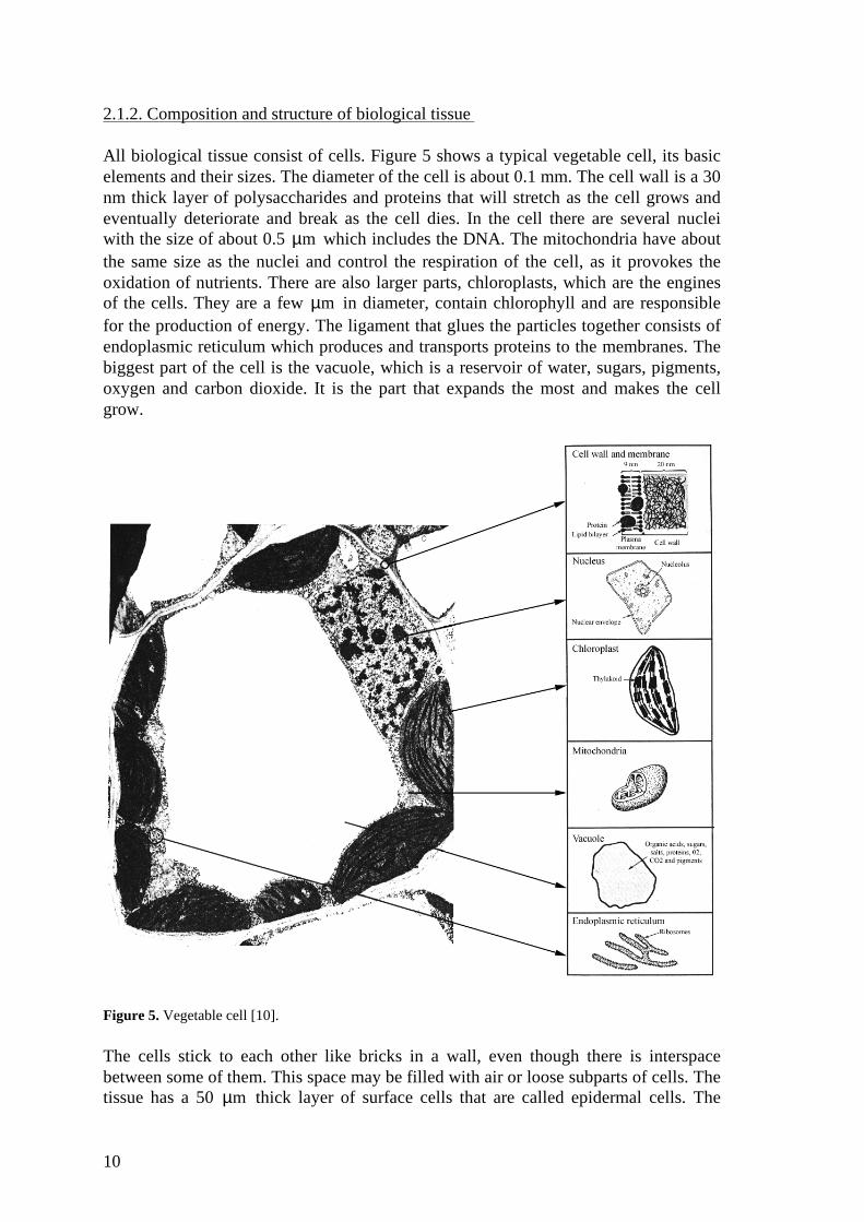
All biological tissue consist of cells. Figure 5 shows a typical vegetable cell, its basicelements and their sizes. The diameter of the cell is about 0.1 mm. The cell wall is a 30nm thick layer of polysaccharides and proteins that will stretch as the cell grows andeventually deteriorate and break as the cell dies. In the cell there are several nucleiwith the size of about 0.5 µm which includes the DNA. The mitochondria have aboutthe same size as the nuclei and control the respiration of the cell, as it provokes theoxidation of nutrients. There are also larger parts, chloroplasts, which are the enginesof the cells. They are a few µm in diameter, contain chlorophyll and are responsiblefor the production of energy. The ligament that glues the particles together consists ofendoplasmic reticulum which produces and transports proteins to the membranes. Thebiggest part of the cell is the vacuole, which is a reservoir of water, sugars, pigments,oxygen and carbon dioxide. It is the part that expands the most and makes the cellgrow.

Figure 5. Vegetable cell [10].

The cells stick to each other like bricks in a wall, even though there is interspacebetween some of them. This space may be filled with air or loose subparts of cells. Thetissue has a 50 µm thick layer of surface cells that are called epidermal cells. The

11

surface is normally covered with wax, small fluff called trichomes and pigments tomoderate the wavelengths that penetrate it. Leaves which have been extensivelystudied have more layers. Their next layer is called palisade and is about 1 mm thick.Underneath is the spongy layer which has about the same thickness [11].

The distribution of chloroplasts is not homogenous right the way through the tissue. Ithighly depends on the type of vegetable and where it grows. When it grows in theshade and is reached by diffuse light, it needs another distribution than if it receivesdirect collimated light. It also has a movement of the chloroplasts, called cyclosis, toadjust the absorption of light. There is even a movement of whole cells to use the lightas effectively as possible. As the light penetrates the tissue, the intensity decreaseswith the depth and the cells turn towards the highest gradient of the light. In otherwords, the biological tissue is not a “vegetable” , it is actively working to influencelight propagation and absorption to its own advantage.

2.1.3. Optical properties of biological tissue

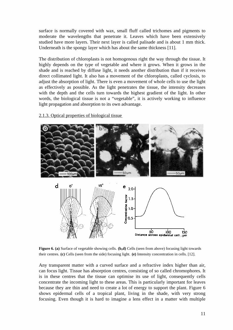
Figure 6. (a) Surface of vegetable showing cells. (b,d) Cells (seen from above) focusing light towards

their centres. (c) Cells (seen from the side) focusing light. (e) Intensity concentration in cells. [12].

Any transparent matter with a curved surface and a refractive index higher than air,can focus light. Tissue has absorption centres, consisting of so called chromophores. Itis in these centres that the tissue can optimise its use of light, consequently cellsconcentrate the incoming light to these areas. This is particularly important for leavesbecause they are thin and need to create a lot of energy to support the plant. Figure 6shows epidermal cells of a tropical plant, living in the shade, with very strongfocusing. Even though it is hard to imagine a lens effect in a matter with multiple

12

scattered light, calculations of radiation within maize mesocotyls, the first leaves of thesprout, indicate that focusing further into the tissue could exist [5]. Obviously theelectromagnetic field in biological tissue is very heterogeneous and the concentrationsof light vary a lot.

Let us now reason microscopically about the scattering with the above mentionedtypes of interactions with matter; reflection, scattering and absorption. As the tissuehas a higher refractive index than air, there will be a reflection on the surface. Thelight that penetrates however, may therefore also be trapped inside. If polarised light isused, it will loose its polarisation at a high exponential rate as it penetrates the tissue.Therefore approximately all the light that is reflected back with kept polarisationcomes from the reflection in the surface [4,5]. During a study, when illuminatingbiological tissue with polarised light, researchers found that the polarisation in thespecular direction of observation was 0.98 due to the reflection in the surface but only0.17 in a 0°/30° setup (similar to the one that is used in this study).

The refractive indexes are different inside and outside the cells as well as in all the cellparts and in the cell wall. The indexes of different vegetable cell walls have beeninvestigated with results between 1.333-1.472 and with an average of 1.425 [6]. Thismeans that the back scattered light from biological tissue not only is multiplescattered, but is also multiple reflected on different surfaces.

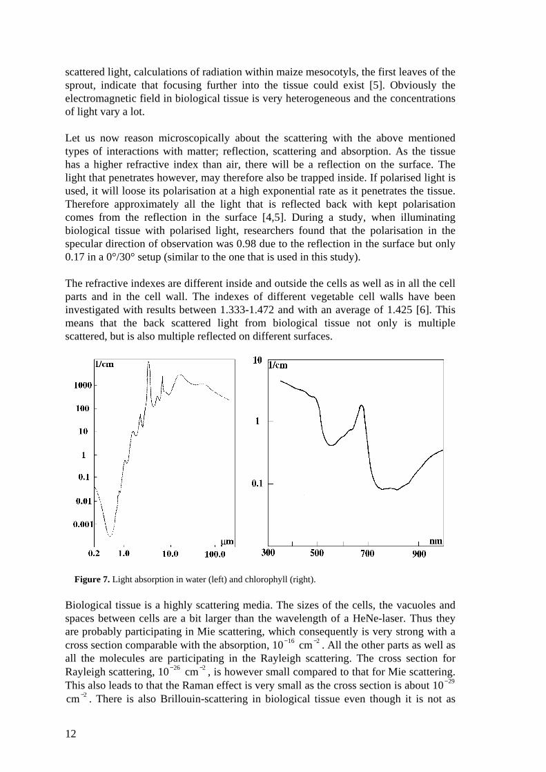
Figure 7. Light absorption in water (left) and chlorophyll (right).

Biological tissue is a highly scattering media. The sizes of the cells, the vacuoles andspaces between cells are a bit larger than the wavelength of a HeNe-laser. Thus theyare probably participating in Mie scattering, which consequently is very strong with across section comparable with the absorption, 10−16 cm−2 . All the other parts as well asall the molecules are participating in the Rayleigh scattering. The cross section forRayleigh scattering, 10−26 cm−2 , is however small compared to that for Mie scattering.This also leads to that the Raman effect is very small as the cross section is about 10−29

cm−2 . There is also Brillouin-scattering in biological tissue even though it is not as

13

strong as in a crystal. These effects will cause direct or indirect shifts and broadeningsin the scattered light. This will be further discussed in chapter 2.4.

The absorption is wavelength dependent and varies a lot. Due to that the mainabsorbers are water and chlorophyll, the absorption spectrum mainly depends on them.In figure 7, the absorption spectra for water and chlorophyll are illustrated. Note thatthey have different scales of wavelength. We can see that water absorbs a lot in theinfrared region, yet it has a window at around 0.6 µm. A HeNe-laser is therefore agood source to use if you do not want to get your signal absorbed by water. Thechlorophyll naturally absorbs of course a lot in the visible range, since that is its mainpurpose. One of the chlorophyll’s absorption peaks coincides with the wavelength ofthe laser, 633 nm. This greatly facilitates measurements of the amount of chlorophyllin an object. When measuring speckles, a strong absorption does not cause importantproblems. However, when measuring an object where the quantity of chlorophyllchanges a lot, changes in the speckle size may occur with time as less absorptioninvolves deeper penetration of the light. By using a diaphragm, it is possible to get ridof this problem since this method keeps the speckle size constant.

Most of the absorbed energy will turn into heat but the change of temperature willprobably not be important even though there is a strong absorption. Let us for examplecalculate how much the energy in the object increases due to the setup I am using inthis study. I illuminate a disc with 2 mm in diameter and a thickness of about 3 mm,which is approximately 0.0012 ⋅ π⋅ 0.003⋅1000 kg = 10 mg water, with a 10 mW HeNelaser during about 40 s. Due to an imperfect polariser only 50 % of the laserbeam

reaches the object. The object will hence increase ∆T =∆W

m ⋅ Cv

⋅ 0.5

K =

10⋅10−3 ⋅ 40

10⋅10−6 ⋅ 4.18⋅103⋅ 0.5

K = 5 K in temperature. However, this approximation assumes

that no light is neither scattered nor reflected from the object. Furthermore, there willbe convection with the rest of the object as well as the air and the object will radiateenergy from its surface. All together the increased temperature will be limited to only afew Kelvin.

Photon

g=0g=0.5

g=0.8

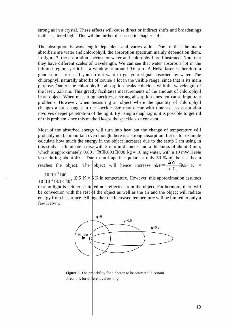
Figure 8. The probability for a photon to be scattered in certain

directions for different values of g.

14

The most common way of describing the properties of a medium is with the absorptioncoefficient, µa , and scattering coefficient, µs. To get the total coefficient, the two arecoupled to define the linear transport coefficient µ tr = ′ µ s + µa . ′ µ s is the reducedscattering coefficient ′ µ s = (1− g)µs which depends on the anisotropy factor g. g is themean cosine of the scattering angle and can obtain values between -1 and 1. g=1 ispure forward scattering and g=0 is uniform scattering, figure 8. Human tissue, forexample, has a typical value of the factor g=0.7-0.95 [13]. To get an idea of thecoefficients in a strawberry I mention some experimental values for a cotyledon ofcucurbita pepo, which is a leaf; µa=0.8 mm−1 and µs=2.2 mm−1.

These coefficients will however not be used in this work. The scattering is of fargreater importance than the absorption and it is instead necessary to differ the types ofscatterings included in µs from each other.

15

2.2. Speckles

2.2.1. Laser speckles

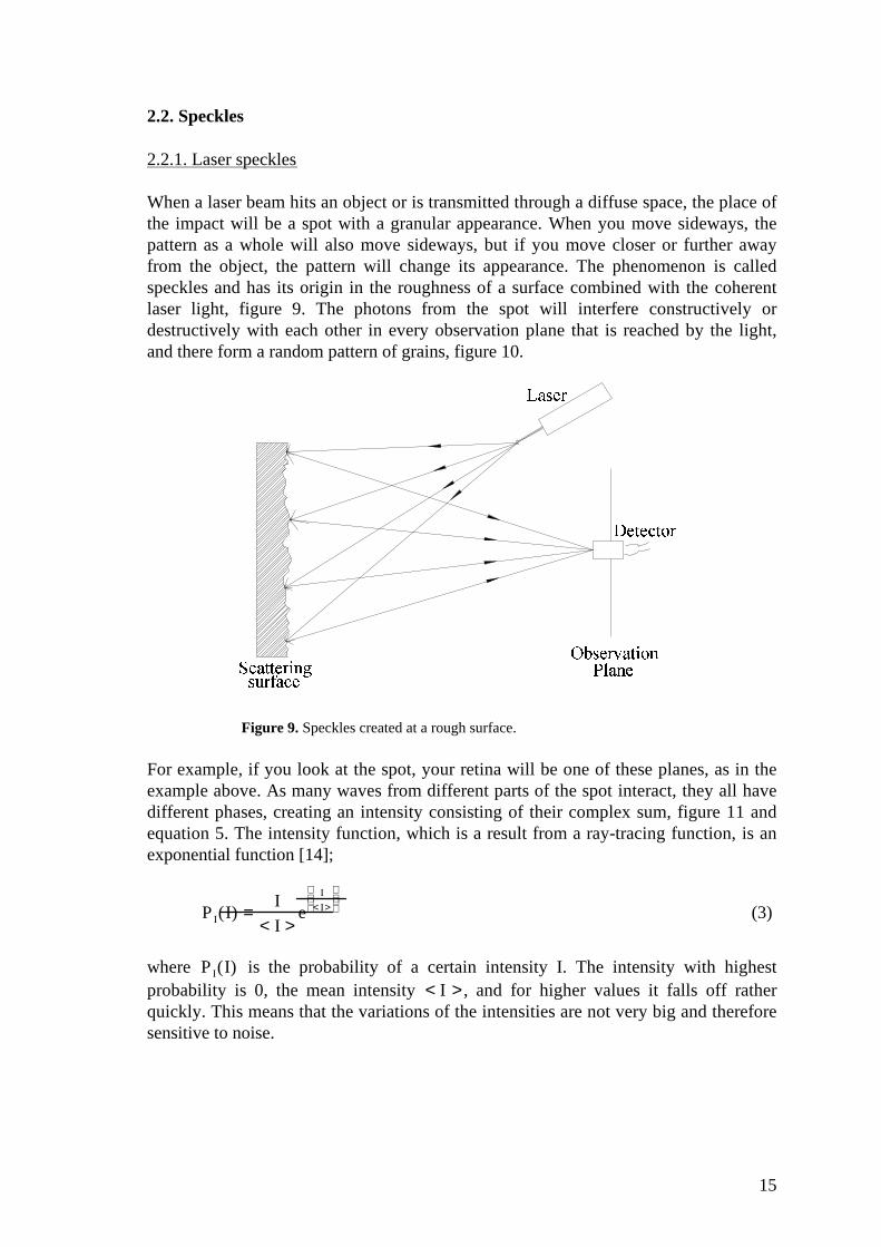
When a laser beam hits an object or is transmitted through a diffuse space, the place ofthe impact will be a spot with a granular appearance. When you move sideways, thepattern as a whole will also move sideways, but if you move closer or further awayfrom the object, the pattern will change its appearance. The phenomenon is calledspeckles and has its origin in the roughness of a surface combined with the coherentlaser light, figure 9. The photons from the spot will interfere constructively ordestructively with each other in every observation plane that is reached by the light,and there form a random pattern of grains, figure 10.

acbed bgf!d h�i

jlknm,boi

prq m,boits�k3dtu�h�vwyx�kevzb{ fnk!d|d boi�u�vz}m�~8i���k�f�b

Figure 9. Speckles created at a rough surface.

For example, if you look at the spot, your retina will be one of these planes, as in theexample above. As many waves from different parts of the spot interact, they all havedifferent phases, creating an intensity consisting of their complex sum, figure 11 andequation 5. The intensity function, which is a result from a ray-tracing function, is anexponential function [14];

PI(I) =I

< I >e

I

< I>

(3)

where PI(I) is the probability of a certain intensity I. The intensity with highestprobability is 0, the mean intensity < I >, and for higher values it falls off ratherquickly. This means that the variations of the intensities are not very big and thereforesensitive to noise.

16

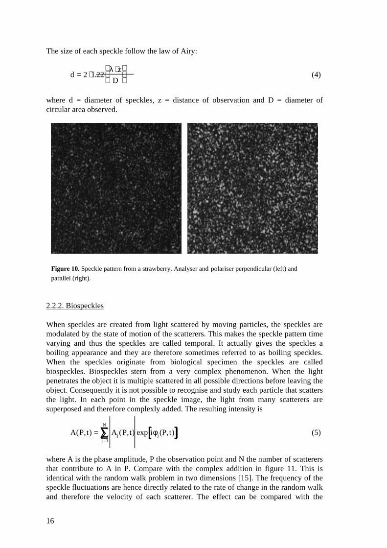
The size of each speckle follow the law of Airy:

d = 2 ⋅1.22λ ⋅ z

D

(4)

where d = diameter of speckles, z = distance of observation and D = diameter ofcircular area observed.

Figure 10. Speckle pattern from a strawberry. Analyser and polariser perpendicular (left) and

parallel (right).

2.2.2. Biospeckles

When speckles are created from light scattered by moving particles, the speckles aremodulated by the state of motion of the scatterers. This makes the speckle pattern timevarying and thus the speckles are called temporal. It actually gives the speckles aboiling appearance and they are therefore sometimes referred to as boiling speckles.When the speckles originate from biological specimen the speckles are calledbiospeckles. Biospeckles stern from a very complex phenomenon. When the lightpenetrates the object it is multiple scattered in all possible directions before leaving theobject. Consequently it is not possible to recognise and study each particle that scattersthe light. In each point in the speckle image, the light from many scatterers aresuperposed and therefore complexly added. The resulting intensity is

A(P,t) = A j (P,t) exp iφj (P,t)[ ]j =1

N

∑ (5)

where A is the phase amplitude, P the observation point and N the number of scatterersthat contribute to A in P. Compare with the complex addition in figure 11. This isidentical with the random walk problem in two dimensions [15]. The frequency of thespeckle fluctuations are hence directly related to the rate of change in the random walkand therefore the velocity of each scatterer. The effect can be compared with the

17

Doppler method where a very narrow laser beam illuminates a vessel and the velocity( � ) of the fluid in the vessel is given from the frequency of the fluctuating scatteredlight:

� � � �� � �= − ⋅��π� �

(6)

where K s and K i are the wave vectors for the incident and the scattered light. In ourcase every scatterer has this Doppler phenomenon, but the directions of the movementsdo not matter. Because of the complexity of the scattered light there has not yet beenestablished accurate mathematical methods to describe this. However, the differentwave vectors, velocity vectors and the multiple scattering all together may statisticallybe interpreted as a Doppler broadening of the scattered light [16]. A problem is that apart of the broadening is a pure random signal superposed with the Dopplerbroadening. A method to get rid of this noise is to measure the evolution of manyspeckles and use the mean value of them all. The random signals will then even outresulting in zero, for proof see further down about autocorrelation.

Im

Re

U

Figure 11. The complex sum of rays that create

a spot in a speckle pattern .

2.2.3. Properties of biospeckles

In this work, the two most interesting dimensions of the speckles are size and intensity.The size of the stationary speckles are, as mentioned above, equal to the Airy discresulting from the size of the illuminated area. But what happens with the size of thespeckles as the light penetrates the object and is multiple scattered? Studies have beenconducted to investigate the properties of time varying speckles. It has been shownthat the speckles resulting from scattering inside an object have a smaller average sizethan the ones produced from scattering on the surface [4]. This can easily be explainedwith the expansion of the laser beam as it penetrates the object. As the light isscattered back, it leaves the object through a larger area than where it entered. In otherwords, the Airy law is still valid but with the actual size of the illuminated area ratherthan the width of the laser beam.

18

The speckle pattern is actually superposed of two different patterns. Large speckles,resulting from scattering on the surface and with a large angular dependence, aremodulated by small speckles, from the light from the interior with very weak angulardependence [17]. In article [4], experiments with apples were made and the ratio of thesizes of the speckles was found to be 1:10. The same researcher showed with aperturesthat the speckle size increases with the decreasing diameter of the aperture and alsothat the rate of temporal changes of the speckles decreases with decreasing aperturesize. The time varying effect of the speckles is also stronger far away from thedirection of the specular reflection [4].

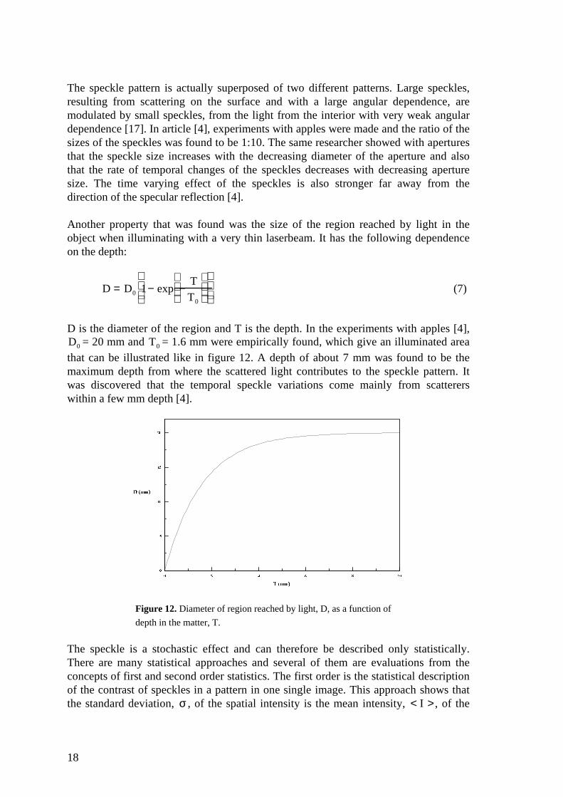
Another property that was found was the size of the region reached by light in theobject when illuminating with a very thin laserbeam. It has the following dependenceon the depth:

D = D0 1− exp −T

T0

(7)

D is the diameter of the region and T is the depth. In the experiments with apples [4],D0 = 20 mm and T0 = 1.6 mm were empirically found, which give an illuminated areathat can be illustrated like in figure 12. A depth of about 7 mm was found to be themaximum depth from where the scattered light contributes to the speckle pattern. Itwas discovered that the temporal speckle variations come mainly from scattererswithin a few mm depth [4].

� � � � � � ��

�

� �

� �

� �

�g� �����

��� �����

Figure 12. Diameter of region reached by light, D, as a function of

depth in the matter, T.

The speckle is a stochastic effect and can therefore be described only statistically.There are many statistical approaches and several of them are evaluations from theconcepts of first and second order statistics. The first order is the statistical descriptionof the contrast of speckles in a pattern in one single image. This approach shows thatthe standard deviation, σ , of the spatial intensity is the mean intensity, < I >, of the

19

speckle pattern. The contrast may be expressed as σ2

< I >2 and when this ratio is 1, the

pattern has a maximum contrast and is therefore fully developed [18]. This of coursedepends on the time the image is exposed. With a very long exposure, the image willbecome unclear, resulting in a very low contrast. However, with the knowledge of thetime, the contrast and the ratio of moving scatterers to stationary ones, it is possible todetermine the mean velocity of the scatterers. This technique can be used for exampleto visualise blood flow in the retina and to study vibrations [18].

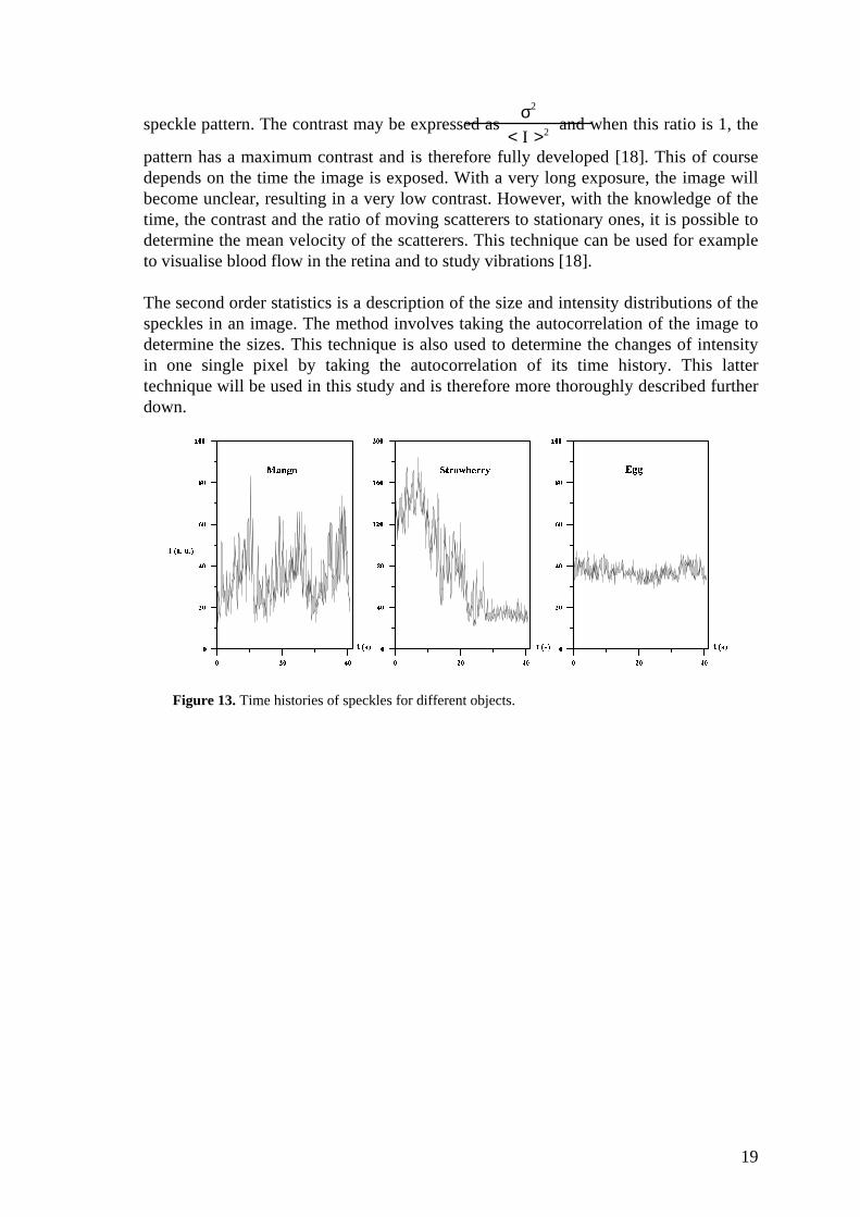
The second order statistics is a description of the size and intensity distributions of thespeckles in an image. The method involves taking the autocorrelation of the image todetermine the sizes. This technique is also used to determine the changes of intensityin one single pixel by taking the autocorrelation of its time history. This lattertechnique will be used in this study and is therefore more thoroughly described furtherdown.

� ��� �*������*��*��*��*�*�

 �¡ ¢¤£=¥¦£ §

¨ª©�«t¬�­

® ¯�® °*®®°*®±*®² ¯�®²*³*®¯�®*®

´ µ¤¶�·�¸3¹�º�¶�¶¦»

¼ ½�¼ ¾*¼¼½�¼¾*¼¿*¼À*¼Á*¼*¼

Â5Ã�Ã

Ä|Å Æ ÇÄ|Å Æ ÇÄ|Å Æ Ç

Figure 13. Time histories of speckles for different objects.

20

2.3. Autocorrelation and the Wiener-Khinchin theorem

A way of studying the evolution of speckles is to record the time history of itsintensity. Figure 13 shows a typical time histories of speckles. In order to extract theinformation from the variations, it is common to take the autocorrelation of the timehistory, figure 14. The autocorrelation, γ(t) , is a technique to determine how theevolution correlates with itself [14];

γ(t) =1

< I2 >I(τ ) ⋅I (τ − t)dτ

−∞

∞

∫ . (8)

I(t) is the time history function and 1

< I 2 > the normalising factor. For example, if a

specific sequence of a variation appears a few times during the time history of thespeckle, the autocorrelation will show a strong correlation for the entire duration ofthat sequence. After this sequence, the different parts of the time evolution will crosscorrelate with each other making the autocorrelation randomly stay around the meanvalue of the signal.

È É È È É Ê È É Ë È É Ì È É Í Î É È Î É ÊÈ É È

È É Ê

È É Ë

È É Ì

È É Í

Î É È

Ï�ЦÑ�Ð

Ò�Ó Ô Õ

Ö Ò ×¤ØÚÙ-Û�Ü�פ×�ÝÞ Ø¦ß�à=á

Figure 14. Autocorrelations of time histories of speckles for

different objects.

As I have mentioned earlier, there is always a stationary speckle pattern that issuperposed with the temporary evolution. To obtain only the fluctuations we subtractthe mean value of the intensity. This means that we will have a time history that variesaround the mean value zero and an autocorrelation that goes down to zero when thecross correlating begins. The correlation time, τ c , can be defined as the time it takesfor the normalised autocorrelation function to drop to for example 1/e or 1/2 ofmaximum. The smaller the value τ c is, the faster the movement in the speckle patternis.

21

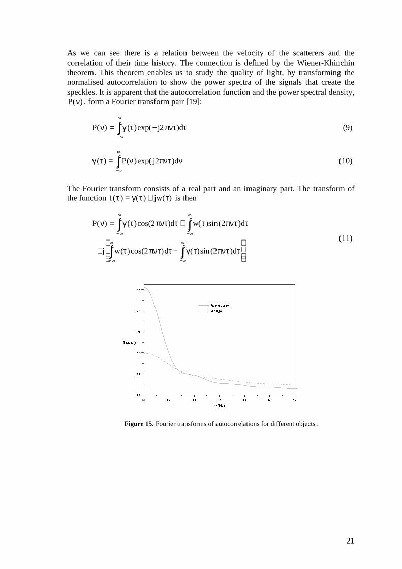
As we can see there is a relation between the velocity of the scatterers and thecorrelation of their time history. The connection is defined by the Wiener-Khinchintheorem. This theorem enables us to study the quality of light, by transforming thenormalised autocorrelation to show the power spectra of the signals that create thespeckles. It is apparent that the autocorrelation function and the power spectral density,P(ν) , form a Fourier transform pair [19]:

P(ν) = γ(τ )exp(− j2πντ)dτ−∞

∞

∫ (9)

γ(τ ) = P(ν)exp( j2πντ)dν−∞

∞

∫ (10)

The Fourier transform consists of a real part and an imaginary part. The transform ofthe function f (τ ) = γ(τ) + jw(τ) is then

P(ν) = γ(τ )cos(2πντ)dτ−∞

∞

∫ + w(τ )sin(2πντ)dτ−∞

∞

∫

+ j w(τ )cos(2πντ)dτ−∞

∞

∫ − γ(τ)sin(2πντ)dτ−∞

∞

∫

(11)

â ã â â ã ä â ã å â ã æ â ã ç è ã â è ã äâ ã â

â ã å

â ã ç

è ã ä

è ã æ

ä ã â

é�ê ë¦ì=í�ì î

ï�ð ñ,ò*ó

ô=õ ö¤÷Úø,ù�ú¤ö¤ö*ûü(÷¦ý�þ¦ÿ

Figure 15. Fourier transforms of autocorrelations for different objects .

22

Since the autocorrelation only has a real part and is an even function, the Fouriertransform will also be a real function and we will end up with [20]

P(ν) = γ(τ )cos(2πντ)dτ−∞

∞

∫ = 2 ⋅ γ(τ )cos(2πντ)dτ0

∞

∫ (12)

This means that we can work with half the functions all the time, which saves a lot ofspace. There will always be an imaginary part in the calculations, it can hence beignored.

Figures 14 and 15 show the autocorrelations and their Fourier transforms of imagesfrom three different fruits. As we can see, a short correlation time is the result of fastchanges in the speckle pattern and hence a high frequency in the Fourier transform.From the power function we can extract the mean velocity of the scatterers with

v =∆ω2

1

w+

σ2

∆x2

−1/ 2

=1

τ c

1

w+

σ2

∆x2

−1/2

(13)

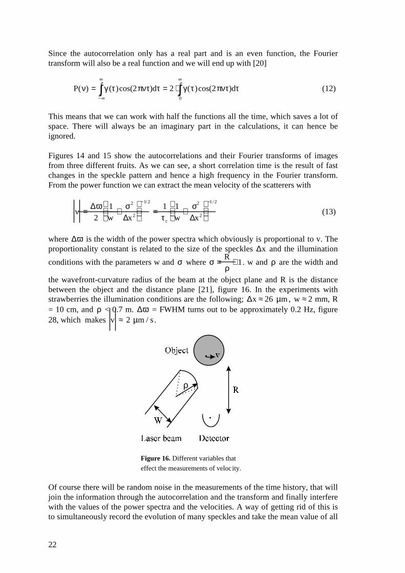
where ∆ω is the width of the power spectra which obviously is proportional to v. Theproportionality constant is related to the size of the speckles ∆x and the illumination

conditions with the parameters w and σ where σ =R

ρ+1. w and ρ are the width and

the wavefront-curvature radius of the beam at the object plane and R is the distancebetween the object and the distance plane [21], figure 16. In the experiments withstrawberries the illumination conditions are the following; ∆x ≈ 26 µm, w ≈ 2 mm, R= 10 cm, and ρ < 0.7 m. ∆ω = FWHM turns out to be approximately 0.2 Hz, figure28, which makes v ≈ 2 µm / s.

� � � � � � � �� � � � � � �

� � � � �

�

�

ρ

Figure 16. Different variables that

effect the measurements of velocity.

Of course there will be random noise in the measurements of the time history, that willjoin the information through the autocorrelation and the transform and finally interferewith the values of the power spectra and the velocities. A way of getting rid of this isto simultaneously record the evolution of many speckles and take the mean value of all

23

the autocorrelations. For example one can use an array of 512 pixels as I have done inthis study. An example of such an intensity evolution is shown in figure 17. This willlevel the noise to a zero everywhere in the autocorrelation except for t=0.

Figure 17. Images of 512 timehistories each, when measuring a strawberry (left) and a dead object

(right).

To prove this, we calculate the effect of random noise in the autocorrelation of a timehistory. The time history of every pixel has changing intensity, I, at any given time(Any single frame taken by the image processor) decided by the activity in the speckleintensity ̂ I , modulated by the random intensity I (t) − ˆ I :

A(t) = I1(t) − ˆ I 1( )⊗ I 2(t) − ˆ I 2( )=

I1(t) ⊗ I2(t) − I1(t) ⊗ ˆ I 2 − ˆ I 1 ⊗ I 2(t) + ˆ I 1 ⊗ ˆ I 2

(14)

In order to perform this autocorrelation we must take a few relations intoconsideration:

I1(t) and I 2(t) are two random intensities which therefore are independent:

P I1 I 2( )= P I1( ). (15)

24

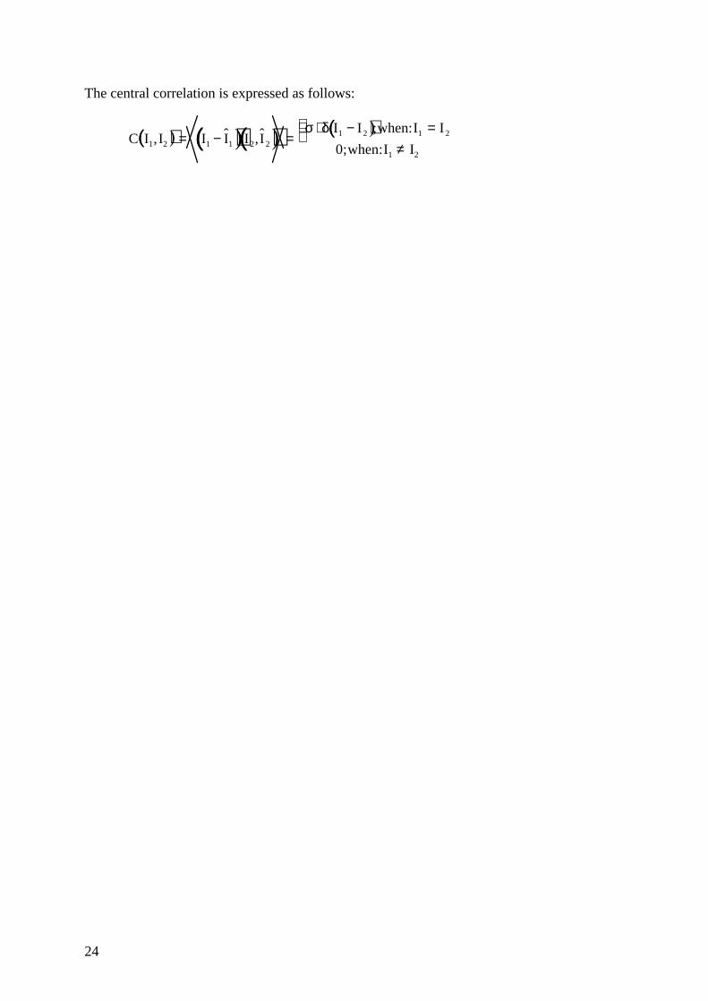
The central correlation is expressed as follows:

C I1,I2( ) = I1 − ˆ I 1( ) I 2,ˆ I 2( ) =

σ ⋅ δ I1 − I 2( );when:I1 = I 2

0;when:I1 ≠ I2

î (16)

Let us now express every mean value of a time history of a pixel in the speckle patternas a constant times the window. The window is a rectangle that lasts as long as thepixel is measured, a time constant here denoted b:

ˆ I (t) = ˆ I ⋅ rectt

b

. (17)

We then find that the autocorrelation above can be expressed as:

A(t) = I1(t) ⊗ I 2(t) − ˆ I 2 I1(t) ⊗ rectt

b

−ˆ I 1 I 2(t) ⊗ rectt

b

+ ˆ I 1 ⋅ ˆ I 2 ⋅ rect

t

b

⊗ rect

t

b

(18)

In the processing of the image, we take the mean value of 512 autocorrelations:

ˆ A (t) =< I1(t) ⊗ I 2(t) > −ˆ I 1 ⋅ˆ I 2 ⋅ rectt

b

⊗ rect

t

b

−ˆ I 1 ⋅ˆ I 2 ⋅ rectt

b

⊗ rect

t

b

+ ˆ I 1 ⋅ ˆ I 2 ⋅ rect

t

b

⊗ rect

t

b

(19)

According to the central correlation, this is zero everywhere except when I1 = I 2 . Thisgives us

< I1(t) ⊗ I2(t) >= ˆ I 1 ⋅ ˆ I 2 ⋅ rectt

b

⊗ rectt

b

(20)

which shows that the mean value of many autocorrelations of the total signal is themean value of the signal without noise. However one detail remains. In A(0) we willobtain a peak which contains the total signal including noise.

σ ⋅ δ(0) =< I 2(0) > −ˆ I 2 (21)

Since the mean intensity in these experiments is subtracted from the measured values,this leaves us with the autocorrelation function γ tot (t) = γ(t) + σ ⋅δ(t) . The Fouriertransform is then Ptot (ν) = P(ν) + σ which means that there will always be a small

constant bias due to noise in the power spectra. The size of the constant, σ =< I n2 >,

will be studied further down, when discussing the limits of the equipment.

25

2.4. The line profile and its origin

The variations of the speckles depend, as I mentioned earlier, on the phase changes ofthe many different rays of light that compose it. The probability of the different phasesis a rectangle function and does therefore not effect the shape of the line width [22].Many of the rays are superposed and if there is a convolution it may be hard todistinguish different line shapes from each other. For instance, different gaussianshapes combine their widths, making another gaussian one. On the other hand, whenworking with autocorrelations and Fourier transform, it is beneficial to use thefollowing property of the convolution [20]:

G(α ) ⋅ H(ν − α)dα−∞

∞

∫ = G(ν)∗ H(ν) = F g(t) ⋅ h(t)( ) (22)

In other words, a convolution in the frequency domain is a product in the time domain.The most dominant effects that create the line profile are Doppler, Turbulence andDiffusion. In order to understand the changes in the line profile, those effects aredescribed below:

2.4.1. The Doppler effect

The frequency of photons scattered from moving particles will be modified dependingon the speed of the moving parts. An illustration of the effect is the sound of the carson the highway changing in frequency between coming towards you and going awayfrom you. This is called the Doppler effect, which is closely related to the process inthe time varying speckles. However in the speckle pattern, the fluctuation is mainlycaused by interference of many rays rather than shifts in single photons. According tothe central limit theorem, independent stochastic variables have approximately anormal distribution as long as the number of trials is large. Assuming that the randommovements of the many scatterers are independent, they obey the normal distributionand hence the Gaussian one [3].

Unlike the Doppler method, the direction of the movements of the scatterers are of noconsequence to the speckle pattern. Both effects cause the same frequencies andbroadenings and they both appear in the time varying speckles. The intensityfluctuation is however more dominated by the random phase variation due tointerference than by the Doppler shift of photons, and therefore it is more correctlycalled time varying speckle phenomenon.

The measure I use for the Doppler width is the Full Width at Half Maximum (FWHM).Having determined this dimension it is easy to calculate the mean speed of thescatterers with equation 13. This mean value contains the broadenings from all typesof scattering in all types of particles in the matter. Therefore small changes in one typeof broadening may not even be noticeable in the resulting signal. In this study, Iassume that the part of Doppler in the line shape is dominant and I thereforeapproximate the FWHM for Doppler broadening with FWHM for the results.

26

2.4.2. Turbulence

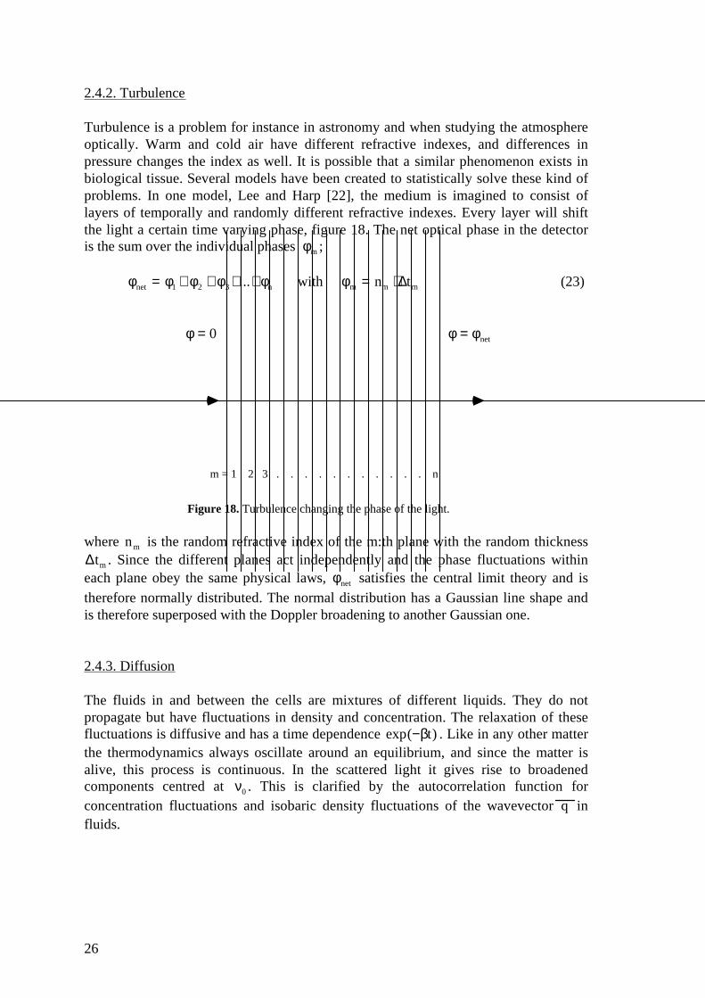
Turbulence is a problem for instance in astronomy and when studying the atmosphereoptically. Warm and cold air have different refractive indexes, and differences inpressure changes the index as well. It is possible that a similar phenomenon exists inbiological tissue. Several models have been created to statistically solve these kind ofproblems. In one model, Lee and Harp [22], the medium is imagined to consist oflayers of temporally and randomly different refractive indexes. Every layer will shiftthe light a certain time varying phase, figure 18. The net optical phase in the detectoris the sum over the individual phases φm ;

φnet = φ1 + φ2 + φ3+...+φn with φm = nm ⋅ ∆tm (23)

φ = 0 φ = φnet

m = 1 2 3 . . . . . . . . . . . n

Figure 18. Turbulence changing the phase of the light.

where nm is the random refractive index of the m:th plane with the random thickness∆tm . Since the different planes act independently and the phase fluctuations withineach plane obey the same physical laws, φnet satisfies the central limit theory and istherefore normally distributed. The normal distribution has a Gaussian line shape andis therefore superposed with the Doppler broadening to another Gaussian one.

2.4.3. Diffusion

The fluids in and between the cells are mixtures of different liquids. They do notpropagate but have fluctuations in density and concentration. The relaxation of thesefluctuations is diffusive and has a time dependence exp(−βt) . Like in any other matterthe thermodynamics always oscillate around an equilibrium, and since the matter isalive, this process is continuous. In the scattered light it gives rise to broadenedcomponents centred at ν0 . This is clarified by the autocorrelation function forconcentration fluctuations and isobaric density fluctuations of the wavevector q influids.

27

The return to the equilibrium concerning the concentration, C(t,r), is given by

∂C

∂t= D∇ 2C (24)

where D is the diffusion coefficient.The return to the equilibrium concerning the isobaric density, ρ(t, r) , is given by

∂ρ∂t

p

= χ∇ 2ρ (25)

where χ is the thermal diffusivity.The autocorrelation functions for fluctuations of the wave vector q in fluids are then,according to [23],

γC(τ) =< Cq2 > exp −D ⋅q2 τ( ) (26)

γρ(τ ) =< ρq

2> exp −χ ⋅q2 τ( ) (27)

The Fourier transform of an exp(−βτ) is β

β2 + ν2 which is a Lorentzian line shape.

This will hence be the result of the fluctuations in concentration and density in theobject. Of course there will be many different diffusions in biological tissue, resultingin a series of Lorentzians with different line widths all centred at ν0 with an addedtotal line width. A convolution between them is an addition of their diffusion constantsin the autocorrelation.

2.4.4. The Voight profile

In a lot of optic and spectroscopy research one encounters the Voight profile. Thisprofile is a convolution of a Gaussian line shape and a Lorentzian line shape. One canthink of it as if every single Doppler-element were smeared out into a Lorentzianprofile. Actually there are usually several different Lorentzian and Gaussiancontributions to the shape. The Lorentzian for instance is normally a combination ofpressure broadening and natural broadening. The resulting Lorentzian width of manycontributions result in

δνL = δνL 1 + δνL 2+...+δνLN . (28)

28

The corresponding relation for the Gaussian line shape, when several velocity shiftswith different speed combines, is [24]

δνD( )2= δνD1( )2

+ δνD2( )2+...+ δνDN( )2

. (29)

The greatest difference between the two shapes is that the Lorentzian profile has widerwings than the Gaussian one. This results in that the wings of the Voight profile almostentirely are decided by the Lorentzian, irrespective of its contribution. For example, atthe double FWHM only 0,2 % of the Gaussian peak is represented compared to 6 % ofthe Lorentzian peak [24]. On the other hand, the central part and the FWHM of the lineprofile are almost entirely determined by the Gaussian contribution. This fact is usedwhen calculating the ratio of Lorentzian to Gaussian width (yL / D )

Optical transfer in the atmosphere is an example of when the Voight profile can beapplied. At sea level the line shape is almost pure Lorentzian but 30 km up in the airthe relationship is 50/50. In this case the Lorentzian shape is pressure dependent andthe Gaussian one depends on the Doppler shift of the radiators, in other words thetemperature [25]. Another example is when working with plasma waves and acousticsin astrophysics. The mathematical functions describing the profile is in this case thesame as in the atmosphere but the physical reasons are different.

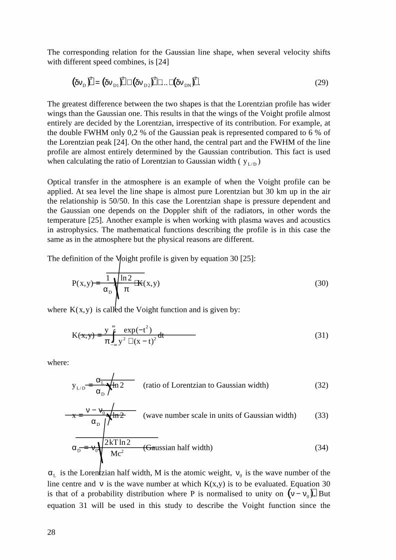
The definition of the Voight profile is given by equation 30 [25]:

P(x,y) =1

αD

ln2

π⋅ K(x,y) (30)

where K(x,y) is called the Voight function and is given by:

K(x,y) =y

πexp(−t2)

y2 + (x − t)2−∞

∞

∫ dt (31)

where:

yL / D =αL

αD

ln 2 (ratio of Lorentzian to Gaussian width) (32)

x =ν − ν0

αD

ln2 (wave number scale in units of Gaussian width) (33)

αD = ν0

2kT ln2

Mc2(Gaussian half width) (34)

αL is the Lorentzian half width, M is the atomic weight, ν0 is the wave number of theline centre and ν is the wave number at which K(x,y) is to be evaluated. Equation 30is that of a probability distribution where P is normalised to unity on ν − ν0( ). But

equation 31 will be used in this study to describe the Voight function since the

29

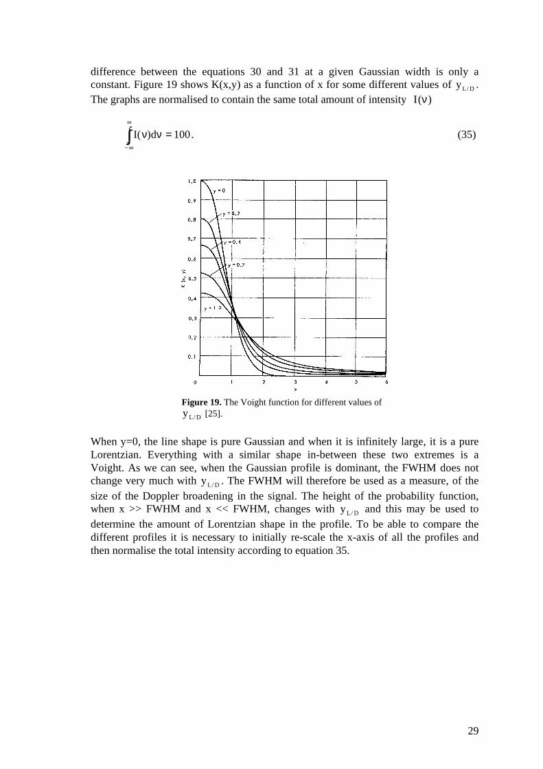
difference between the equations 30 and 31 at a given Gaussian width is only aconstant. Figure 19 shows K(x,y) as a function of x for some different values of yL / D .The graphs are normalised to contain the same total amount of intensity I (ν)

I(ν)dν = 100−∞

∞

∫ . (35)

Figure 19. The Voight function for different values of yL / D [25].

When y=0, the line shape is pure Gaussian and when it is infinitely large, it is a pureLorentzian. Everything with a similar shape in-between these two extremes is aVoight. As we can see, when the Gaussian profile is dominant, the FWHM does notchange very much with yL / D . The FWHM will therefore be used as a measure, of thesize of the Doppler broadening in the signal. The height of the probability function,when x >> FWHM and x << FWHM, changes with yL / D and this may be used todetermine the amount of Lorentzian shape in the profile. To be able to compare thedifferent profiles it is necessary to initially re-scale the x-axis of all the profiles andthen normalise the total intensity according to equation 35.

30

2.4.5. Other broadenings and shifts

The line shape is not only dependent on the different broadenings but also on differentshifts and inelastic scattering effects which interfere with the elastically scattered light.The large shifts do not effect the measurements in this study because they changefaster than the slow speed of the equipment. The time that elapses between therecording of two frames of images is 80 ms. This means that the highest frequency that

will be measurable is 1

0.080 s−1 =12.5 Hz, which corresponds to

f

c⋅10−2 =

12.5

3⋅108⋅10−2

cm−1 = 4 ⋅10−10 cm−1 . Everything that changes with a higher rate, or has a bigger shiftor broadening, will be recorded as random noise. Therefore the Raman scatteringwhich normally has shifts between 100-1000 cm−1 [21] is not noticeable. Even if itwould have had small shifts, the cross section for Raman is very small, one milliontimes smaller than for fluorescence, and is therefore not detectable in this studyanyway.

Fluorescence of absorbed energy may be of the same frequency but has a delay in thens region. That is about the time it takes for the wave package to pass as a whole,keeping the waves from interfering with each other apart from randomly. TheBrillouin-scattering is probably one of the most important effects that will disturb themeasurements. Acoustic waves with a frequency of a few hertz will not be audiblewith the human ear but may vibrate the setup. Let us imagine a very rough model ofthe object, a 3 cm wide crystal consisting of proteins. An estimation of the lowest

phonon frequency possible in the object is ν =vo

λ=

103

3⋅10−2= 33 kHz, where vo is the

approximate velocity of sound in the object, which is a far too high frequency to benoticeable in this work. Lower frequencies will show as displacements of the objectunless if the detector moves with it. The setup as a whole may however have resonancefrequencies in the region of our measurements. These vibrations and displacementsmay be transmitted from the building through the ground or the air. The walls andfloors of a building undergo mostly shear and bending vibrations which usuallyresonate at frequencies between 15 and 25 Hz. The buildings may transfer or beexcited by vibrations from for example machines with frequencies typically between10 and 100 Hz, ventilation ducts typically between 6 and 65 Hz and people walkingand working in laboratories typically in the range of 1 to 3 Hz [26]. Typical floorvibration amplitudes are between 10−7 and 10−6 m [27] which is about ten times largerthan the wavelength used in this work and therefore of great importance.

Raman scattering and fluorescence will not greatly influence the measurements. If theexperiments were combined with spectroscopy one would probably be able to extractmore information because of all the shifts that are specific for the object. However,considering the level of this study, should these factors interfere, they will only benoise among the broadenings due to Doppler, index shift and diffusion. The Brillouin-scattering, however, is obviously the most important source of noise in this work andneed to be considered when evaluating the results of the measurements.

31

2.5. The development of strawberries

The development of strawberries is very unusual because they, unlike most otherfruits, continue to increase in weight throughout the development including theripening. Furthermore, the developing process of strawberries is visually apparent.They change in colour, softness and flavour as well as in size. The whole process lastsfor only a few weeks depending strongly on the environment, especially thetemperature. The ripening part happens fast with a very short time of optimumcondition of the fruits. The definitions of the different stages that have been usedamong researchers, and for the sake of continuity also will be used here, are: smallgreen (SG), large green (LG), white (W), pink (P), red (R) and dark red (DR)[28,29,30]. Since the development is a relatively fast process, the different phases mayoverlap, making the studies of them more difficult.

The initial growth after petal fall is due to a combination of cell division and cellexpansion. After about a week, the cell multiplication is completed and replaced by aperiod of growth during which the cells only increases in volume. The expansion isinfluenced by the turgor pressure and correlates with concentration of solutesincluding sugar [31]. The strawberry grows to a size according to the number of cellsthat have been created at first. Which size the strawberry finally reaches, depends ongenetic factors and is correlated with the number of seeds it has.

Sugar content (mg/g fresh weight) Sugar flow ( � g/min)

Stage Free spaceCytoplasm

Vacuole Total P M T P

Largegreen 5.7 ± 0.3 4.0 ± 0.4 35.2 ±

0.944.8 ±

1.6487 ± 8 293 ± 45

Pink 10.0 ±0.1

12.1 ±1.6

52.9 ±4.0

75.0 ±5.7

570 ± 4 84 ± 5

Table 1. Sugar content in cells and sugar flow through cellular membranes at two stages of the

development of strawberries. P M is the plasma membrane and T P the tonoplast, which is the

membrane around the vacuole [31].

As the cell enlarges, it is accompanied by major changes in the cell wall and the subcellular structure. At petal fall the cells have dens walls and small vacuoles. Whengrowing, the disorganisation increases and the fruit obtains a softer structure. Thesoftening process, as well as the post harvest shelf life, depend very much on thechange of the cell walls. Therefore this has been extensively studied [28,29].Nevertheless, researchers still do not agree on what causes the degradation of the cellwall. It is for certain though, that the wall composition changes as it grows. Italternates polymers which results in an overall increase in the proportion of lowmolecular weight polymers [28]. This makes the tissue unable to maintain its structural

32

integrity since the components of the wall are less tightly bound. When the cell finallybreaks, the contents of the vacuole smear out between all the other cells making thetissue even softer.

Sugar is needed to provide energy for the metabolic changes that constantly occur.Sucrose, glucose and fructose constitutes 99 % of all the sugar in the fruit, 83 % beingglucose and fructose [30]. The process of sugar accumulation is still poorly understoodbut it more or less diffuses through the strawberry to reach every cell. It is known thatthe sugar composition varies with the degree of ripeness. The growth rate of thestrawberry actually correlates with the sugar uptake. Most of the imported sugaraccumulates in the vacuole which contains more than 70 % of the total amount ofsugar [31]. Table 1 shows the sugar content and velocity through membranes at twodifferent stages of the development. It is evident that the flow of sugar through thetonoplast into the vacuole is higher as the strawberry is green. As the strawberry turnsred however, the cells break and cause a strong flow of subparts of cells, includingsugar.

t (days)

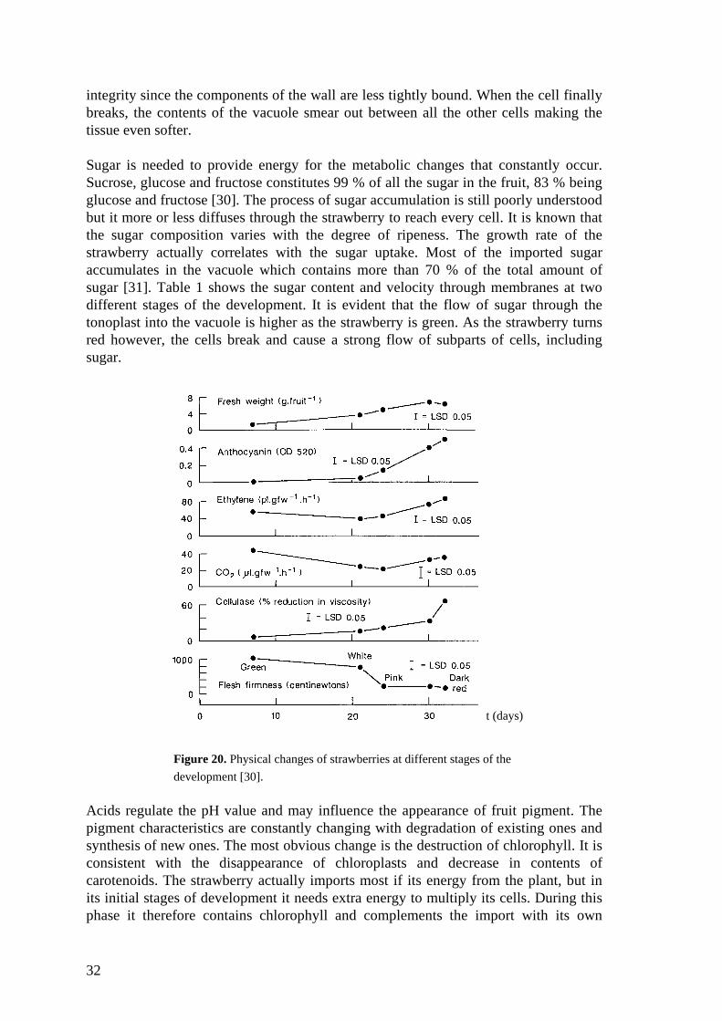
Figure 20. Physical changes of strawberries at different stages of the

development [30].

Acids regulate the pH value and may influence the appearance of fruit pigment. Thepigment characteristics are constantly changing with degradation of existing ones andsynthesis of new ones. The most obvious change is the destruction of chlorophyll. It isconsistent with the disappearance of chloroplasts and decrease in contents ofcarotenoids. The strawberry actually imports most if its energy from the plant, but inits initial stages of development it needs extra energy to multiply its cells. During thisphase it therefore contains chlorophyll and complements the import with its own

33

photosynthesis. Finally the strawberry turns red in order to attract animals to eat it, andthereby spread the seeds.

All these changes in the strawberry; the different movements of cells and the varioussubparts, the changes in colours and the diffusion of sugar, water and cell shape duringthe development may influence the interaction with light. An important change shouldfor instance appear as the cells brake and the vacuoles start to leak. The effects it mayhave on the signal is described above in chapter 2.4. The changes in some of thedifferent stages can be seen in figure 20.

34

35

3. Experimental study

3.1. Introduction

The objective of the experimental work was to find a relationship between the signals,obtained from the scattered light, and the changes in the process of maturing fruit. Theequipment was investigated and optimised in order to find the limits of theexperiments and the possibility of stretching them. Before the real measurementsstarted, it was necessary to find out which fruits were suitable enough to measure. Itwas also interesting to study how the signals differ with the different macroscopiccharacteristics of fruits. A great number of fruits, with different characteristics, weretherefore measured. The strawberry turned out to be a suitable fruit for themeasurements of maturation for many reasons. Bearing in mind that the maturationprocess of the strawberry is very fast, the activity was not too fast to register. Theobvious visible changes of the strawberry that occur and reveal the stage of maturationare also very important. Furthermore, the small potted strawberry plants are easy tocarry in and out of the laboratory. Two experimental setups were used. The first one,called setup A, was used during the experiments with different fruits and pilot tests ofthree strawberries. The second setup, called setup B, was used during the experimentsof the rest of the strawberries as well as the tests of the equipment.

3.2. The experimental setup and equipment

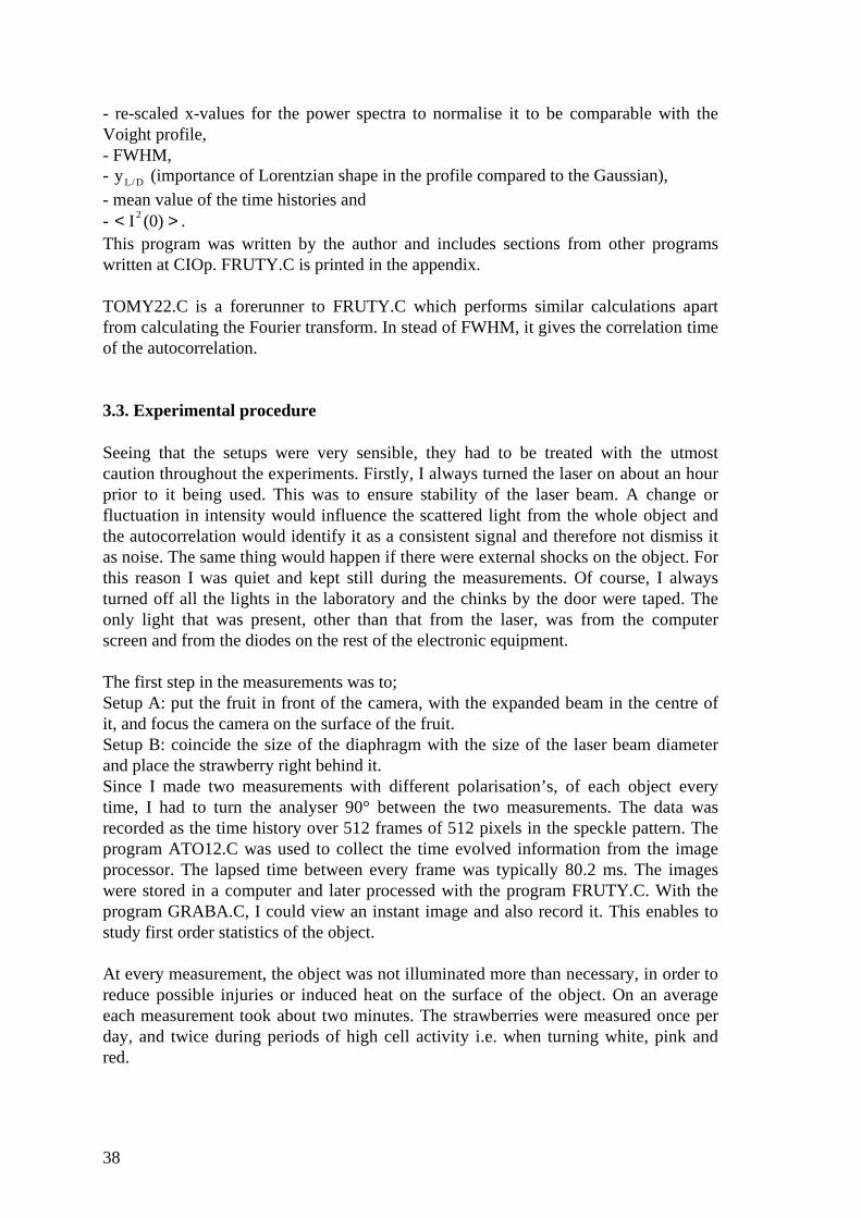
3.2.1. Setup A: With an expanded laser beam and without a diaphragm.

The setup is illustrated in figure 21. The camera is focused on the surface of the object.To fill the whole image with a speckle pattern, diameter 10 mm, the laser beam isexpanded with a lens. This setup did however turn out to have some characteristicswhich could be improved. It was hard to be in control of the focusing as the surfaces ofthe fruits never were completely even and the intensity distribution on the surface wasnot constant. Due to the curvature of the object it is also hard to control the angle ofincident and reflected light. The speckle size also varied with the depth of thepenetration of light and were always very small. Setup A was therefore exchanged forsetup B after the experiments with different fruits and a pilot test with threestrawberries.

3.2.2. Setup B: With a normal laser beam and with a diaphragm.

This setup is illustrated in figure 22. The changes compared to setup A is that the laserbeam is not expanded and there is a diaphragm with diameter 2 mm in front of theobject which is a size close to the diameter of the laser beam. This makes it possible tocontrol the size of the speckles and limit the detection of light scattered deep into thetissue, without limiting the intensity of incoming light. The camera now has anextension on the objective enabling it to focus very close to the camera lens. Theimage on this plane in front of the camera consists of a pattern of large speckles, all

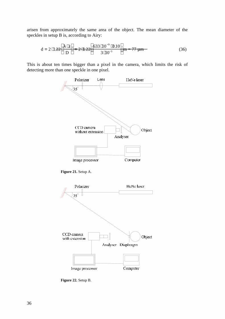
36

arisen from approximately the same area of the object. The mean diameter of thespeckles in setup B is, according to Airy:

d = 2 ⋅1.22λ ⋅ z

D

= 2 ⋅1.22

633⋅10−9 ⋅ 0.10

3⋅10−3

m = 77 µm (36)

This is about ten times bigger than a pixel in the camera, which limits the risk ofdetecting more than one speckle in one pixel.

�������

���������! #"%$#&��'�(�)$*" + $*�, #-#.���"

/0$213�4"6587'��"

9 �:��1<;=�)��"

>?��@A�!13�'�)��"

BDC�E �F&�.+!+HG &F������")�I 58.8J:$*-#.��4K#.������65�$L�

MON

Figure 21. Setup A.

PRQ�SUT�VDW�X%Y�ZUVL[\[(Y*X ] Y*Q^W#_2`�VFX

abY*c3SFX6d<eLVFX

f?g SFcihj[(VFX

klV4mnVDcoSL[(VFX

prq4s VUZt`uld8SFW�v�X%S�T2Q

]w] uxZUSFQ�VFX6Sy dz`ovnVt{#`�V g [|d8Y g

}�~

Figure 22. Setup B.

37

3.2.3. Equipment

The laser is a 632.8 nm HeNe-laser with an output of 10 mW single mode TEM00 . Itcomes from Melles Griot and is called 05-LHP-991. It has an angular drift of less than0.03 mrad after 15 min and a noise amplitude of less than 0.5 %.

The camera is a PULNIX TM-560 No 010038. It has a detection plate that consists of512 x 512 pixels. The lens has the f number 1:1.4, the diameter 16 mm and the outerdiameter 25.5 mm. The lens is extended with a 40 mm COSMICAR TV-lens extensiontube in setup B. The camera sends images to the image processor at a maximum rate of50 Hz.

The image processor is an ADI-151 from Imaging Technology Inc. It digitisesincoming imagery from video inputs and stores it momentarily in two sets of archives(512 x 512). It has a signal-to-noise ratio greater than 40 dB. When testing the speed ofthe grabbing, it was acknowledged that the processor registers frames at 12.5 Hz whichtherefore is the highest frequency that can be detected. The program, ATO12.C, wasmodified to register only a few pixels of the image from the camera to make theprocessor faster. However it turns out that it is necessary to skip many pixels so as toget a higher rate of registration. The loss of accuracy due to fewer pixels is for thisreason not worth the small increase in frequency of the registration. This modificationwas therefore not used in the final ATO12.C. Since the time history of a pixel isrecorded during 512*80.2 ms = 41 s, the lowest frequency that will be recorded is 24mHz.

3.2.4. Computer programs

Many different computer programs were used in the many pilot tests performed duringthe course of the experimental study. I will however only mention the most importantones:

ATO12.C is the name of the program that controls the image processor and stores theimages in the computer. It was written at CIOp a few years ago and works well withthe rest of the equipment.

GRABA.C takes as snapshot of the image in the camera.

VOIGHT.FOR is used to calculate Voight profiles. The input is a file of x-values andthe output is a file of yL / D -values thus forming the profile. It can be found in [25].

FRUTY.C is a program that removes the head from the image file, subtracts the meanvalue of the time history of each pixel, autocorrelates the 512 time histories and takesthe mean autocorrelation of them all as well as Fourier transforms the autocorrelation.The following data is obtained for every image:- files of autocorrelation,- Fourier transform,

38

- re-scaled x-values for the power spectra to normalise it to be comparable with theVoight profile,- FWHM,- yL / D (importance of Lorentzian shape in the profile compared to the Gaussian),- mean value of the time histories and- < I 2(0) > .This program was written by the author and includes sections from other programswritten at CIOp. FRUTY.C is printed in the appendix.

TOMY22.C is a forerunner to FRUTY.C which performs similar calculations apartfrom calculating the Fourier transform. In stead of FWHM, it gives the correlation timeof the autocorrelation.

3.3. Experimental procedure

Seeing that the setups were very sensible, they had to be treated with the utmostcaution throughout the experiments. Firstly, I always turned the laser on about an hourprior to it being used. This was to ensure stability of the laser beam. A change orfluctuation in intensity would influence the scattered light from the whole object andthe autocorrelation would identify it as a consistent signal and therefore not dismiss itas noise. The same thing would happen if there were external shocks on the object. Forthis reason I was quiet and kept still during the measurements. Of course, I alwaysturned off all the lights in the laboratory and the chinks by the door were taped. Theonly light that was present, other than that from the laser, was from the computerscreen and from the diodes on the rest of the electronic equipment.

The first step in the measurements was to;Setup A: put the fruit in front of the camera, with the expanded beam in the centre ofit, and focus the camera on the surface of the fruit.Setup B: coincide the size of the diaphragm with the size of the laser beam diameterand place the strawberry right behind it.Since I made two measurements with different polarisation’s, of each object everytime, I had to turn the analyser 90° between the two measurements. The data wasrecorded as the time history over 512 frames of 512 pixels in the speckle pattern. Theprogram ATO12.C was used to collect the time evolved information from the imageprocessor. The lapsed time between every frame was typically 80.2 ms. The imageswere stored in a computer and later processed with the program FRUTY.C. With theprogram GRABA.C, I could view an instant image and also record it. This enables tostudy first order statistics of the object.

At every measurement, the object was not illuminated more than necessary, in order toreduce possible injuries or induced heat on the surface of the object. On an averageeach measurement took about two minutes. The strawberries were measured once perday, and twice during periods of high cell activity i.e. when turning white, pink andred.

39

3.4. Study of noise

3.4.1. Introduction

When working with speckles there will always be random movements that do not addany information about the object but that will disappear in a mean value of manymeasurements. There will also be error due to fluctuations or movements due to theequipment and the surroundings. By estimating the source and amount of noise presentin the measurements, it is possible to either reduce the noise producing factors or toestimate the reliability of the results. Tests were done with each and every part of theequipment. I simply added one part of the equipment after the other, and studied theamount of noise for each combination and determined if the noise was random or not.When checking the camera, it was covered with a thick black cloth to prevent anyincoming light. The laser was kept off until the dead objects were about to bemeasured.

3.4.2. Results

Piece of equipmentadded to the setup

Correlationtime (ms)

< I2 (0) > (au)

Image processor (Impr1) 0 0Cord Impr-Camera (Cord1) 0 0Camera covered (Cam1) 1.02 1.76Camera covered (Cam2) 1.02 1.75Camera uncovered (Cam3) 1.02 1.75Camera uncovered (Cam4) 1.01 1.74Dead object (Dead1) 1.36 6.94Dead object (Dead2) 1.05 2.69Dead object (Dead3) 1.40 3.52Dead object (Dead4) 1.04 1.49Strawberry 1 18.21 310Strawberry 2 16.88 306

Table 2. Noise depending on different parts of the equipment. The names in

parenthesis are the names of the files of data.

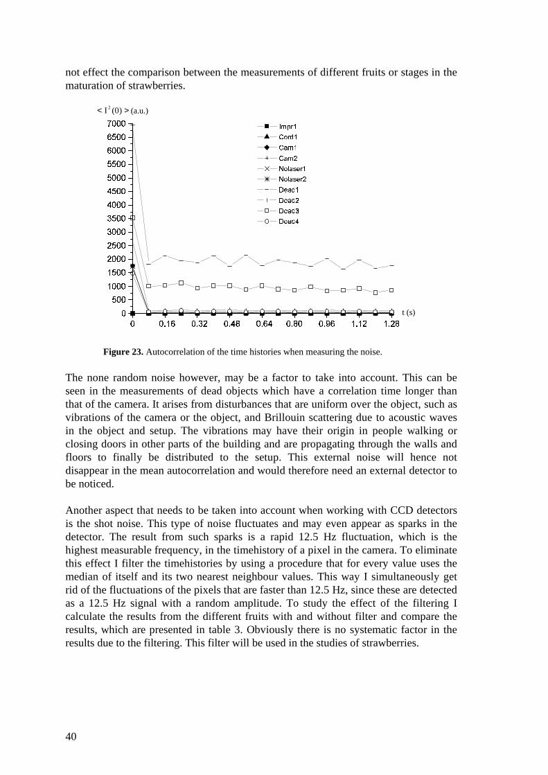
Table 2 shows the different combinations that were measured and their respectivecorrelation times and values of < I 2(0) > . The autocorrelations are also presented in amore pedagogical way in figure 23. As we can see there is no noise until the camera isconnected. The measurements of absolute dead objects are also very similar to theones for only the camera. It is hence obvious that most of the noise comes from thecamera. Since the autocorrelation drops directly after the t = 0 and after that decreaseslinearly, the noise is fully random according to the proof mentioned earlier, equation20. The height of the delta is the value of < I 2(0) > . This is to be compared with thevalues of < I 2(0) > for the measurements of fruits. It turns out that the signal to noiseratio at t = 0 is about 1000, which is enough for what is necessary in this study.Furthermore, if the random noise is believed to have constant mean intensity it does

40

not effect the comparison between the measurements of different fruits or stages in thematuration of strawberries.

< I 2 (0) > (a.u.)

� �j�z�t� �j� �2� �j� �#� �j� �L� �:� �*� �:� �*� �L�<��� �L� �*���2�*����2�2����2�2��*�2�2��*�2�2��*�2�2��*�2�2����2�2����2�2��*�2�2��*�2�2��*�2�2��*�2�2��*�2�2� � ���\�i�

��� � �'���� �H���� �0������ �|�)� �<������ �|�)� � ����\� �'����\� �4����\� �t����\� �4�

t (s)

Figure 23. Autocorrelation of the time histories when measuring the noise.

The none random noise however, may be a factor to take into account. This can beseen in the measurements of dead objects which have a correlation time longer thanthat of the camera. It arises from disturbances that are uniform over the object, such asvibrations of the camera or the object, and Brillouin scattering due to acoustic wavesin the object and setup. The vibrations may have their origin in people walking orclosing doors in other parts of the building and are propagating through the walls andfloors to finally be distributed to the setup. This external noise will hence notdisappear in the mean autocorrelation and would therefore need an external detector tobe noticed.

Another aspect that needs to be taken into account when working with CCD detectorsis the shot noise. This type of noise fluctuates and may even appear as sparks in thedetector. The result from such sparks is a rapid 12.5 Hz fluctuation, which is thehighest measurable frequency, in the timehistory of a pixel in the camera. To eliminatethis effect I filter the timehistories by using a procedure that for every value uses themedian of itself and its two nearest neighbour values. This way I simultaneously getrid of the fluctuations of the pixels that are faster than 12.5 Hz, since these are detectedas a 12.5 Hz signal with a random amplitude. To study the effect of the filtering Icalculate the results from the different fruits with and without filter and compare theresults, which are presented in table 3. Obviously there is no systematic factor in theresults due to the filtering. This filter will be used in the studies of strawberries.

41

Fruit FWHM(Hz)

FWHM withfilter (Hz)

yL / D yL / D

with filterPumpkin 0.365 0.365 1.013 1.038Banana 0.365 0.365 0.971 0.973Chirimoya 0.146 0.146 0.733 0.709Egg 0.073 0.073 0.388 0.353Lettuce 0.146 0.146 0.649 0.619Mango 0.341 0.341 1.048 1.024

Table 3. Comparison between calculations with and without filter.

The effect the total noise has on the width of the Lorentzian shape is bigger than thaton the FWHM of the Gaussian one, equations 28 and 29, which must be taken intoaccount when evaluating the results of the measurements.

42

3.5. Study of the line profile of light scattered in different fruits and vegetables

3.5.1. Introduction

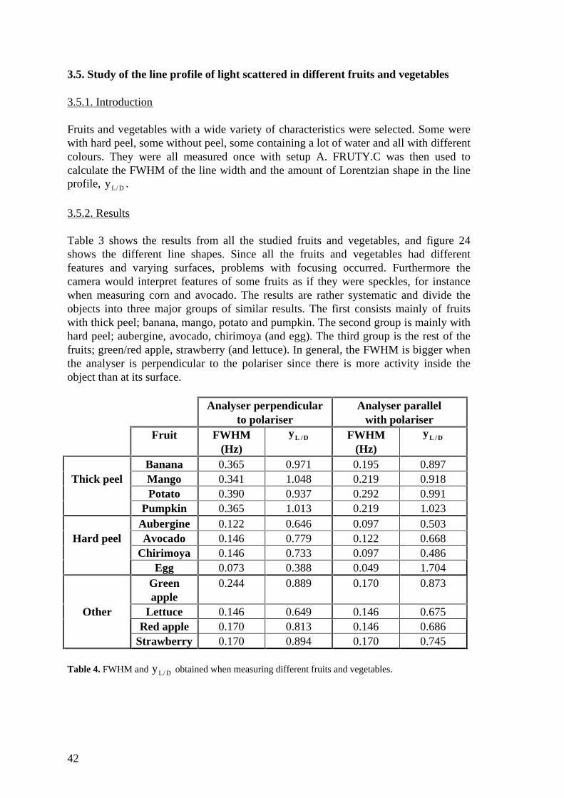
Fruits and vegetables with a wide variety of characteristics were selected. Some werewith hard peel, some without peel, some containing a lot of water and all with differentcolours. They were all measured once with setup A. FRUTY.C was then used tocalculate the FWHM of the line width and the amount of Lorentzian shape in the lineprofile, yL / D .

3.5.2. Results

Table 3 shows the results from all the studied fruits and vegetables, and figure 24shows the different line shapes. Since all the fruits and vegetables had differentfeatures and varying surfaces, problems with focusing occurred. Furthermore thecamera would interpret features of some fruits as if they were speckles, for instancewhen measuring corn and avocado. The results are rather systematic and divide theobjects into three major groups of similar results. The first consists mainly of fruitswith thick peel; banana, mango, potato and pumpkin. The second group is mainly withhard peel; aubergine, avocado, chirimoya (and egg). The third group is the rest of thefruits; green/red apple, strawberry (and lettuce). In general, the FWHM is bigger whenthe analyser is perpendicular to the polariser since there is more activity inside theobject than at its surface.

Analyser perpendicularto polariser

Analyser parallelwith polariser

Fruit FWHM(Hz)

yL / D FWHM(Hz)

yL / D

Banana 0.365 0.971 0.195 0.897Thick peel Mango 0.341 1.048 0.219 0.918

Potato 0.390 0.937 0.292 0.991Pumpkin 0.365 1.013 0.219 1.023

Aubergine 0.122 0.646 0.097 0.503Hard peel Avocado 0.146 0.779 0.122 0.668

Chirimoya 0.146 0.733 0.097 0.486Egg 0.073 0.388 0.049 1.704

Greenapple

0.244 0.889 0.170 0.873

Other Lettuce 0.146 0.649 0.146 0.675Red apple 0.170 0.813 0.146 0.686

Strawberry 0.170 0.894 0.170 0.745

Table 4. FWHM and yL / D obtained when measuring different fruits and vegetables.

43

� �2� �2�  2� ¡t�2� ¡t�2� ¡t�*� ¡t 2� �2�2� �2�2� �2�2��j¢ ��j¢z¡�j¢ ��j¢ £�j¢ ¤�j¢ ��j¢ ¥�j¢  

¦�§4¨(©�ª «t¬ ­(©¦L®%¯4°)±(²t¯³U±t­(±�­(±´:µ(¬ ª ¬ ¶b¯|·)±¸F«4«¹=ª ©4©t­(±tº4º\» ©¼(©)½ ½¾§(°)©¿=±t­%«t¯ÀU¯|½ ±|½ ¯\©ÀL§4¶�º4Á6¬ ­Â�©(²t±tº4º\» ©Ã�½¾ª ±%Ä=¨(©tª¾ª ·

Å3ÆÈÇÊÉUË

ÌUÅ8ÍjÎ ÏOÎ Ë

ν

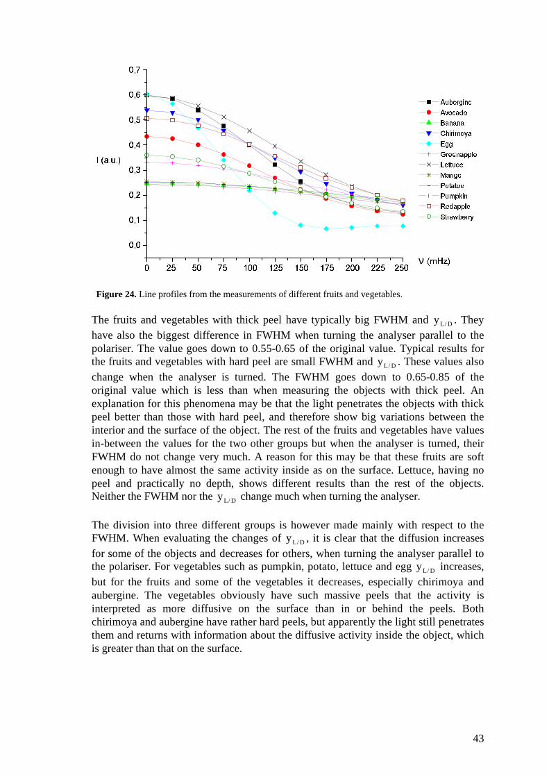
Figure 24. Line profiles from the measurements of different fruits and vegetables.

The fruits and vegetables with thick peel have typically big FWHM and yL / D . Theyhave also the biggest difference in FWHM when turning the analyser parallel to thepolariser. The value goes down to 0.55-0.65 of the original value. Typical results forthe fruits and vegetables with hard peel are small FWHM and yL / D . These values alsochange when the analyser is turned. The FWHM goes down to 0.65-0.85 of theoriginal value which is less than when measuring the objects with thick peel. Anexplanation for this phenomena may be that the light penetrates the objects with thickpeel better than those with hard peel, and therefore show big variations between theinterior and the surface of the object. The rest of the fruits and vegetables have valuesin-between the values for the two other groups but when the analyser is turned, theirFWHM do not change very much. A reason for this may be that these fruits are softenough to have almost the same activity inside as on the surface. Lettuce, having nopeel and practically no depth, shows different results than the rest of the objects.Neither the FWHM nor the yL / D change much when turning the analyser.

The division into three different groups is however made mainly with respect to theFWHM. When evaluating the changes of yL / D , it is clear that the diffusion increasesfor some of the objects and decreases for others, when turning the analyser parallel tothe polariser. For vegetables such as pumpkin, potato, lettuce and egg yL / D increases,but for the fruits and some of the vegetables it decreases, especially chirimoya andaubergine. The vegetables obviously have such massive peels that the activity isinterpreted as more diffusive on the surface than in or behind the peels. Bothchirimoya and aubergine have rather hard peels, but apparently the light still penetratesthem and returns with information about the diffusive activity inside the object, whichis greater than that on the surface.

44

3.6. Study of the line profile of light scattered in strawberries during maturation

3.6.1. Introduction

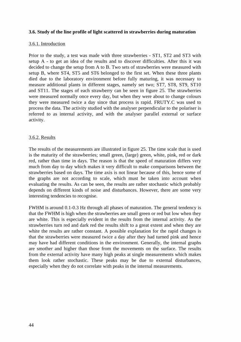
Prior to the study, a test was made with three strawberries - ST1, ST2 and ST3 withsetup A - to get an idea of the results and to discover difficulties. After this it wasdecided to change the setup from A to B. Two sets of strawberries were measured withsetup B, where ST4, ST5 and ST6 belonged to the first set. When these three plantsdied due to the laboratory environment before fully maturing, it was necessary tomeasure additional plants in different stages, namely set two; ST7, ST8, ST9, ST10and ST11. The stages of each strawberry can be seen in figure 25. The strawberrieswere measured normally once every day, but when they were about to change coloursthey were measured twice a day since that process is rapid. FRUTY.C was used toprocess the data. The activity studied with the analyser perpendicular to the polariser isreferred to as internal activity, and with the analyser parallel external or surfaceactivity.

3.6.2. Results

The results of the measurements are illustrated in figure 25. The time scale that is usedis the maturity of the strawberries; small green, (large) green, white, pink, red or darkred, rather than time in days. The reason is that the speed of maturation differs verymuch from day to day which makes it very difficult to make comparisons between thestrawberries based on days. The time axis is not linear because of this, hence some ofthe graphs are not according to scale, which must be taken into account whenevaluating the results. As can be seen, the results are rather stochastic which probablydepends on different kinds of noise and disturbances. However, there are some veryinteresting tendencies to recognise.

FWHM is around 0.1-0.3 Hz through all phases of maturation. The general tendency isthat the FWHM is high when the strawberries are small green or red but low when theyare white. This is especially evident in the results from the internal activity. As thestrawberries turn red and dark red the results shift to a great extent and when they arewhite the results are rather constant. A possible explanation for the rapid changes isthat the strawberries were measured twice a day after they had turned pink and hencemay have had different conditions in the environment. Generally, the internal graphsare smother and higher than those from the movements on the surface. The resultsfrom the external activity have many high peaks at single measurements which makesthem look rather stochastic. These peaks may be due to external disturbances,especially when they do not correlate with peaks in the internal measurements.

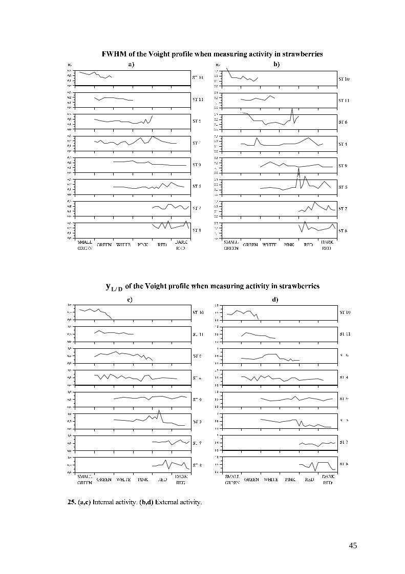
45

Ð�ÑÓÒÕÔ×Ö�Ø0Ù)Ú0ÛrÜÈÖ�Ý3Þ:ÚßÙ�à0áUÖ�Ø6Ýoâ3Ûäã^Ú0Û'åçæèÛ'é:ê�ëbáUÝ3å0Þ^éOìUÙ)ÝiíjÝiÙ6î�Ý3åïê\Ù(áUé#ã^ð=Û*áLáUÝoÛLêñ4ò óLô õ4ö ÷#ø

ù ú ú û ú ú ü ú ú ý ú ú þ ú ú ÿ ú ú � ú úú � úú � ùú � ûú � ü

�����

�����

���

�����

��� �

��� �

�������

�������

������������������ � !"�#%$&� �'�(&�'�)� !��*+��,),

(&���)�-!

. / / 0 / / 1 / / 2 / / 3 / / 4 / / 5 / // 6 // 6 ./ 6 0/ 6 1

. / / 0 / / 1 / / 2 / / 3 / / 4 / / 5 / // 6 // 6 ./ 6 0/ 6 1

. / / 0 / / 1 / / 2 / / 3 / / 4 / / 5 / // 6 // 6 ./ 6 0/ 6 1

. / / 0 / / 1 / / 2 / / 3 / / 4 / / 5 / // 6 // 6 ./ 6 0/ 6 1

. / / 0 / / 1 / / 2 / / 3 / / 4 / / 5 / // 6 // 6 ./ 6 0/ 6 1

. / / 0 / / 1 / / 2 / / 3 / / 4 / / 5 / // 6 // 6 ./ 6 0/ 6 1

. / / 0 / / 1 / / 2 / / 3 / / 4 / / 5 / // 6 // 6 ./ 6 0/ 6 1

7 8 8 9 8 8 : 8 8 ; 8 8 < 8 8 = 8 8 > 8 88 ? 88 ? 78 ? 98 ? :

@�A�B

@�A�C

@DA�E

@�A�F

@�A G

@DA�H

@�A�I�I

@�AJILK

M�NPO�QO�R)MO�R�MS T U"QV%W&T AXRY&O�R�R-U@DZ[N�\�\

YPO�R-R-U

] ^ ^ _ ^ ^ ` ^ ^ a ^ ^ b ^ ^ c ^ ^ d ^ ^^ e ^^ e ]^ e _^ e `

] ^ ^ _ ^ ^ ` ^ ^ a ^ ^ b ^ ^ c ^ ^ d ^ ^^ e ^^ e ]^ e _^ e `

] ^ ^ _ ^ ^ ` ^ ^ a ^ ^ b ^ ^ c ^ ^ d ^ ^^ e ^^ e ]^ e _^ e `

] ^ ^ _ ^ ^ ` ^ ^ a ^ ^ b ^ ^ c ^ ^ d ^ ^^ e ^^ e ]^ e _^ e `

] ^ ^ _ ^ ^ ` ^ ^ a ^ ^ b ^ ^ c ^ ^ d ^ ^^ e ^^ e ]^ e _^ e `

] ^ ^ _ ^ ^ ` ^ ^ a ^ ^ b ^ ^ c ^ ^ d ^ ^^ e ^^ e ]^ e _^ e `

] ^ ^ _ ^ ^ ` ^ ^ a ^ ^ b ^ ^ c ^ ^ d ^ ^^ e ^^ e ]^ e _^ e `

yL/ Df[gih�j%kmlnf[oDp�jqhsr%tPf[g ovuDkxwyjik{z}|~k{� ���JtPovzipy���Ph�o��o�h ��ovz}�'h)t&�[wy�qk�t�t&ovk����� �[�

� � � � � � � � � � � � � � � � � � � � �� � �� � �� � � � � � � � � � � � � � � � � � � � � � � �� � �� � �� � � � � � � � � � � � � � � � � � � � � � � �� � �� � �� � � � � � � � � � � � � � � � � � � � � � � �� � �� � �� � � � � � � � � � � � � � � � � � � � � � � �� � �� � �� � � � � � � � � � � � � � � � � � � � � � � �� � �� � �� � � � � � � � � � � � � � � � � � � � � � � �� � �� � �� � �

�����

�����

�D���

�����

����

�D���

���¡ � 

���¡ �¢

£�¤�¥�¦¥�§)£¥�§)£¨ © ª"¦«%¬&© �'§­&¥�§)§�ª�D®[¤�¯)¯

­P¥�§�§°ª

± ² ² ³ ² ² ´ ² ² µ ² ² ¶ ² ² · ² ² ¸ ² ²² ¹ ²² ¹ ¶± ¹ ²

º » » ¼ » » ½ » » ¾ » » ¿ » » À » » Á » »»  »»  ¿º  » º » » ¼ » » ½ » » ¾ » » ¿ » » À » » Á » »»  »»  ¿º  » º » » ¼ » » ½ » » ¾ » » ¿ » » À » » Á » »»  »»  ¿º  » º » » ¼ » » ½ » » ¾ » » ¿ » » À » » Á » »»  »»  ¿º  » º » » ¼ » » ½ » » ¾ » » ¿ » » À » » Á » »»  »»  ¿º  » º » » ¼ » » ½ » » ¾ » » ¿ » » À » » Á » »»  »»  ¿º  » º » » ¼ » » ½ » » ¾ » » ¿ » » À » » Á » »»  »»  ¿º  »

ÃvÄ Å

ÃvÄÆ

ÃDÄ�Ç

ÃvÄ È

ÃvÄ[É

ÃDÄ�Ê

ÃvÄJË°Ë

Ã�Ä�ËÍÌ

Î�Ï�Ð'ÑÐ�Ò�ÎÐ�Ò)ÎÓ Ô Õ"ÑÖJ×ØÔ ÄXÒÙ&Ð�Ò�Ò-ÕÃ�ÚÛÏ�Ü)Ü

ÙPÐ�Ò�Ò°Õ

Ý Þ Þ ß Þ Þ à Þ Þ á Þ Þ â Þ Þ ã Þ Þ ä Þ ÞÞ å ÞÞ å âÝ å Þ

æÛç"è�é�ê"ëíì�î%ïvð�ñvòXó°ð+ô�õ[ôØöXñD÷Íø{÷ÍñLù�úPû°ü ýÍþ+ÿ������������� ������������������

46

yL / D stays between 0 and 0.8 through the maturation. Since this value is always below1, the Gaussian part of the line profile is at all times greater than the Lorentzian part.Just like the FWHM, yL / D is high when the strawberries are green and has its lowestvalues at late white. Despite this it goes high already when the berries are pink.Another noticeable feature is that all graphs go low at their ends, which indicates thatthe diffusion decreases as the strawberries are turning dry in the laboratory. The resultsdo not change as wildly as the FWHM does at the red phase, which shows that thediffusion changes with the velocity in the object. The changes at white are very small.

FWHM and yL / D during maturation are illustrated in figure 26 in a matrix thatsummarises parts of the analysis above.

�����

�! �" #%$

&'")(�* +-,/.�0�0�1�2 $3$4(5 276 $38

� .92:1 $1�2 $;$<(

Figure 26. Summary of the changes in FWHM and yL / D , due to the internal activity, as

strawberries mature.

The two measures, FWHM and yL / D , are compared in figure 27 to get an idea aboutthe relation between them. Internally, the FWHM and yL / D follow each other throughsmall changes but at the peaks they correspond to each other in opposite directions.This means that the small changes are due to diffusion which contributes positively toboth measures. The peaks are mainly due to velocity changes which gives the inversecontribution to the yL / D . Note that the highest peaks of yL / D appear when thestrawberries are red. These velocity changes may be either a result from the breakageof the cells when the subparts start to flow among the other cells or from when the softstrawberries move sideways and thereby cause a moving speckle pattern. On thesurface however, the FWHM and yL / D hardly follow each other at all. The onlyrelation between these measures is that the (high) peaks in FWHM give opposite peaksin yL / D . Besides this there are tendencies in the yL / D to go in opposite direction fromthe FWHM even at small changes. This tells us that the diffusion is not as important onthe surface as it is inside the fruit.

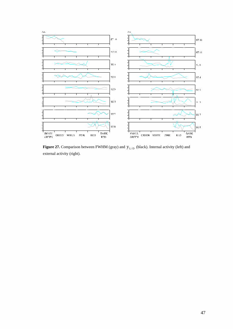
47

=�> ?> =@> ?>

A B B C B B D B B E B B F B B G B B H B B

I�J�K

I�J�L

I�J�M

I�J�N

I J O

I�J�P

I�JRQ�Q

I�JRQ)S

T U V WV X TV X TY Z [ W\ ] Z J X^ V X X [I _ U ` `^ V X X [

a b b c b b d b b e b b f b b g b b h b b

a b b c b b d b b e b b f b b g b b h b b

a b b c b b d b b e b b f b b g b b h b b

a b b c b b d b b e b b f b b g b b h b b

a b b c b b d b b e b b f b b g b b h b b

a b b c b b d b b e b b f b b g b b h b b

a b b c b b d b b e b b f b b g b b h b b

i j j k j j l j j m j j n j j o j j p j j

q�r�s

q r t

q�r�u

q r v

q�r'w

q r x

q�rRyy

q�rRy�z

{ | } ~} � {} � {� � � ~� � � r �� } � � �q � | � �� } � � �

� � � � � � � � � � � � � � � � � � � � �

� � � � � � � � � � � � � � � � � � � � �

� � � � � � � � � � � � � � � � � � � � �

� � � � � � � � � � � � � � � � � � � � �

� � � � � � � � � � � � � � � � � � � � �

� � � � � � � � � � � � � � � � � � � � �

� � � � � � � � � � � � � � � � � � � � �

Figure 27. Comparison between FWHM (gray) and yL / D (black). Internal activity (left) and

external activity (right).

48

49

4. Conclusion and discussion

The line profiles obtained from the Fourier transforms of the autocorrelations of thebiospeckles’ time histories show shifts due to Doppler effect, turbulence and diffusionin the objects. A Voight profile can describe it with FWHM and yL / D as the mainfeatures. With the FWHM it is possible to estimate the average velocity of thescatterers in the objects which turns out to be about 2 µm / s in strawberries. The yL / D

is the ratio of Lorentzian to Gaussian width and a measure of the diffusive movementsin the object. If the laser beam is polarised it is possible to distinct the light scatteredinternally from the light scattered on the surface of the object. Nevertheless, the resultsare rather stochastic but have some interesting tendencies which the conclusions arebased on.

Errors in the measurements are probably due to the changes in the environmentalconditions, for instance temperature and atmospheric pressure, especially during theperiods when the strawberries were measured twice a day. Furthermore, even thoughthe temperature of the object do not increase much due to the laserbeam, it may stillhave an effect on the activity of the object and hence the results of the measurements.This is particularly important on the surface of the object since most light is absorbedthere. The noise from the equipment comes mainly from the camera. It is measured tohave the signal to noise ratio 1000, which is enough for what is necessary in this study.Most of the spectroscopical shifts of the light are too big for the detector and hencerecorded as random noise. However, this type of noise is dismissed by the mean valueof 512 autocorrelations and therefore, it does not interference with the measurements.The most important problem is probably Brillouin scattering due to vibrations anddisplacements transmitted from the building through the ground and the air. Thesevibrations might originate from building vibrations, people working in laboratories andventilation ducts and are in the same range of frequencies as the shifts measured in thisstudy. Some features of the noise were discovered in the experiments. The results fromthe activity on the surface is more stochastic than that from the internal activity. Thenoise has also greater effect on the Lorentzian part of the line profile than the Gaussian(equations 28 and 29), which can be seen in figure 27 where yL / D is more stochasticwhen measured externally than internally.

When different fruits were measured, it was discovered that the results vary with thedifferent characteristics of the objects, but generally there is more activity inside thefruits and vegetables than on their surfaces. The results gave three groups of objectswith similar characteristics, hard peel, thick peel or no peel. Thick peel gives highinternal activity. The objects with neither thick nor hard peel show small differencesbetween internal and external activity. For most of the vegetables the diffusion isgreater on the surface than inside, though this is opposite for the fruits.

The characteristics of the Voight profile from the experiments with strawberries havedifferent features depending on the maturity of the fruit. These results are summarisedin figure 26. Figure 27 compares the two parameters FWHM and yL / D , and shows thatthe activity on the surface mainly depends on the velocity of particles. It also indicatesthat it is possible to detect diffusion on the inside of the fruit, though it is difficult to

50

point out anything specific concerning the diffusion on the surface. When thesetendencies are compared to the sugar flow, table 1, it is discovered that it has very littlecorrelation with the diffusive movements in the strawberries. The flow is very slowwhen the strawberries are pink but, according to the measurements, this is the phase inthe maturation where the diffusion reaches its highest values. When the diffusion wascompared with physical changes in different stages of the maturation (see figure 20),only the flesh firmness was found to correlate with it. This suggests that the diffusionis a result from the movements of the cell walls which are more vivid as the firmnessof the flesh decreases. It can be compared with a crystal of proteins which changes inelasticity. The FWHM correlates well with the amount of CO2 but is probably acombination of the development of CO2 , the transportation of sugar and the changesin viscosity due to cellulose.

Future work in this field could improve and optimise the experiments and dataprocessing in several areas. Primarily the results would probably be better if theenvironment of the strawberries were controlled and preferably constant. Furthermore,it would be interesting to study if the heating of the object due to the laser beam has aneffect on the results. Also to increase the number of samples would probably improvethe results. Further, to optimise the equipment with a faster camera and imageprocessor makes it possible to detect more of the information that the presentequipment dismisses as random noise. Presently it is possible to purchase a camera thattakes 2000 pictures per second. Another possibility would be to use an array ofdetectors, which is faster than a camera. Though, the disadvantage would be that it cannot detect 512 time histories simultaneously. The most important thing to do, however,is to get rid of the noise due to vibrations transferred through the building and thesetup. One alternative would be to hang the setup in rubber straps from the ceiling.The technique eliminates the possibility for the setup to absorb frequencies lower thanthe resonance frequency of the setup, including the straps, which generally swings in afew hertz. This method is used in Scanning Tunnelling Microscopy (STM) and AtomicForce Microscopy (AFM) and can be further studied in [26,27]. To combine theexperiments with spectroscopy would optimise the measurements even more, since thescattering radiates light with much more information than extracted in this study. Thedata processing can also be further optimised. In this work, the measures of the Voightprofile is determined by two very characteristic positions on the line profile.Nevertheless, the profile contains more information that could be extracted if thewhole line profile of the results were used. One example is to make a computerprogram that fits a Voight profile to the experimental results and gives thecharacteristics of it as an output. Another example is to separate the different types ofbroadenings from each other in the autocorrelation, equation 22. In this case, theGaussian shape of the line profile is an e− x2

function, and the Lorentzian an e−x

function.

If the work would be carried out with better equipment, more control of environmentalfactors and a greater amount of samples, it would probably be possible to construct aninstrument to determine the maturity of fruits with the biospeckle technique.

51

Acknowledgements

First of all, I would like to express my most sincere thanks to my supervisor at Centrode Investigaciones Opticas (CIOp), Dr. Héctor J. Rabal, for all his support andengagement during my visit in Argentina, and my supervisor at LTH, Dr. Sven-GöranPettersson. They made this thesis work possible and have been a great help throughoutthe work.

There are many other people at CIOp whose support and friendship I gratefullyacknowledge. I would particularly like to thank Nelly Lucía Cap and Ricardo A.Arizaga, the two computer wizards of the Optics Group.

I would also like to thank Dr. Pedro Marcos Civello at the Centro de Investigaciónes yDesarrollo en Criotecnoligía de Alimentos (CIDCA) at Universidad Nacional de LaPlata (UNLP) for his expertise help in issues concerning strawberries.

Special thanks are due to Joanna Lindbergh and Kristina Steeg for correcting theEnglish in parts of the thesis.

The help and assistance from the Department personnel in Lund is also gratefullyacknowledged.

Finally, I would like to express my appreciation to Lia Zerbino and her family formaking me become a part of their family during my stay in La Plata.

52

53

5. References

[1] Rabal H J, Arizaga R A, Cap N L, Trivi M, Romero G, Alanís E. (1995)”Transient phenomena analysis using dynamic speckle patterns,”Optical engineering vol. 35, no. 1, pp. 57-62.

[2] Ruth B. (1990)”Blood flow determination by the laser speckle method,”Int J Microcirc: Clin Exp 9: 21-45.

[3] Zheng B, Pleass C M, Ih C S. (1994)”Feature information extraction from dynamic biospeckle,”Applied optics vol. 33, no. 2, pp. 231-237.

[4] Xu Z, Joenathan C, Khorana B M. (1995)”Temporal and spatial properties of the timevarying speckles of botanical specimens,” Optical engineering vol. 34, no. 5, pp. 1487-1502.

[5] Vogelmann T C. (1993)”Plant tissue optics,”Annu. rev. plant physiol. plant mol. biol. vol. 44, pp. 231-251.

[6] Gausman H W, Allen W A, Escobar D E. (1974)”Refractive index of plant cell walls,”Applied optics vol. 13, no.1, pp. 109-111.

[7] Tuchin V V. (1993)“Lasers and Fiber Optics in Biomedicine,“Laser Physics vol. 3, no. 4, pp. 767-820.

[8] Svanberg S. (1992)Atomic and molecular spectroscopy, Springer-Verlag.

[9] Bass M. (1995)Handbook of optics I, 2nd ed., McGraw-Hill Inc.

[10] Lehninger A L. (1981)Bioquímica, Las bases moleculares de la estructura y functión celular, 2nd ed. Worth publishers, inc.

[11] Seyfried M, Fukshansky L. (1983)”Light gradients in plant tissue,”Applied optics vol. 22, no. 9, pp. 1402-1408.

[12] Bone R A, Lee D W, Norman J M. (1985)”Epidermal cells functioning as lenses in leaves of tropical rain-forest shade plants,” Applied optics vol. 24, no. 10, pp. 1408-1412.

54

[13] Berg R. (1995)Laser-based cancer diagnostics - Tissue optics considerations,Lund reports on atomic physics, LRAP-184.

[14] Dainty J C, ed. (1975)Laser Speckle and Related Phenomena, Springer-Verlag, Berlin.

[15] Goodman J W, (1984)”Statistical properties of laser speckle patterns,”Laser speckle and related phenomena, Dainty J C, ed., vol 9 of Topics in Applied physics, Springer-Verlag, Berlin, pp. 9-75

[16] Drain L E, (1980)The laser doppler technique chap. 4, p. 70, Wiley, New York.

[17] Briers J D. (1975)”Wavelength dependence of intensity fluctuations in laser speckle patterns

from biological specimens,” Opt. commun. vol. 13, pp. 324-326.

[18] Briers J D. (1993)”Speckle fluctuations and biomedical optics: implications and applications,”Optical engineering vol. 32, no. 2, pp. 277-283.

[19] Goodman J W (1984)Statistical optics.

[20] Gaskill J D. (1978)Linear systems, fourier transforms and optics, p. 193,John Wiley & sons, Inc.

[21] Asakura T, Takai N. (1981)”Dynamic laser speckles and their application to velocity measurements of the diffuse object,” Applied optics vol. 25, no. 3, pp. 179-194.

[22] Friden B R. (1983)Probability, statistical optics, and data testing,Springer-Verlag, Berlin Heidelberg New York.

[23] Cummins H Z, Swinney H L. (1970)Light beating spectroscopy,chap. 3 in Progress in optics vol. VIII, pp. 133-200,, ed. Wolf E

[24] Thorne A P (1988)Spectrophysics, 2nd ed., Chapman & Hall.

[25] Armstrong B H. (1967)”Spectrum line profiles: the voight profile”,J. Quant. Spectrosc. Radiat. Transfer. vol. 7, pp. 61-88, Pergamon Press Ltd.

55

[26] Bai C. (1995)Scanning Tunneling Microscopy and its Application,Springer-Verlag, Berlin Heidelberg.

[27] Wiesendanger R. (1994)Scanning Probe Microscopy and Spectroscopy, methods and applications,Cambridge University Press.

[28] Huber D J. (1984)”Strawberry fruit softening: The potential roles of polyuronides and hemicelluloses,” Journal of food science vol. 49, pp. 1310-1315.

[29] Barnes M F, Patchett B J. (1976)”Cell wall degrading enzymes and the softening of senescent strawberry fruit,”Journal of food science vol. 41, pp. 1392-1395.

[30] Manning K. (1993)Soft fruit, chap. 12 in Biochemistry of fruit ripening,ed. Seymour G, Taylor J, Tucker G, Chapman & Hall, London.

[31] John O-A, Yamaki S. (1994)”Sugar content, compartmentation, and efflux in strawberry tissue,”J. Amer. Soc. Hort. Sci. vol. 119, no. 5, pp. 1024-1028.

56

57

Appendix

/* FRUTY.C */

/* 12-96 */

/* For n number of objects, this program removes the head from a 512x512 imagefile, subtracts the mean value of the time history of each pixel, autocorrelates the 512time histories and takes the mean autocorrelation of them all as well as Fouriertransforms the autocorrelation. The following data is obtained for every image:- files of autocorrelation,- Fourier transform,- re-scaled x-values for the power spectra to normalise it to be comparable with theVoight profile,- FWHM,- yL / D (importance of Lorentzian shape in the profile compared to the amount ofDoppler),- mean value of the time histories and- < I 2(0) > . */

/* This program has the following inputs:For each time the program is run:- name of file containing inputs for every object to process,- name of file for output of mean value of the time histories and- name of file for output of < I 2(0) > .For every object:- name of file containing number and names of images to process,- name of file containing names of output files of autocorrelation,- name of file containing names of output files of Fourier transform,- name of file for output of FWHM and- name of file for output of yL / D . */

/* The images must be in itex or vfg.*/

/* Use FRUTYT.C to check that all the images are OK, so that you will not have abreak in the running of the program */

#include "math.h"#include "stdio.h"#include "fft1opt.h"

main(){long auto1,auto2,g1,g2;float a,v[56],w,vv,nor,g,sum,fwhm,partlor,lorentz,mod,

58

norr,min,meall,hmax,powsum,power,exx,xtot,mre=0,rer=0,rei=0;int lm,p,x,r,j,k,l,q,acom,acome,comp,le[20],length,me,o,m,halfn,z,isign,nn,n,size,size2,xdel,xval,tvax;static int gris[1026],med[513],vect[513];static float autoc[513],prom[1025],data[2050];char nombre1[16],nombre2[16],nombre3[16],nombre4[16],nombre5[16],nombre6[16],nombre7[16],nombre8[16],ca,lw,salida[15],nombre9[16],meansa[16];FILE *arch1,*arch2,*arch3,*arch4,*arch5,*arch6,*arch7,*arch8,*arch9,*meansal,*datsal;

printf("NAME OF FILE FOR OUTPUT OF MEAN VALUES? :\n");scanf("%s",meansa);meansal=fopen(meansa,"w");printf("NAME OF FILE FOR OUTPUT OF < I 2(0) > ? :\n");scanf("%s",nombre9);arch9=fopen(nombre9,"w");printf("NAME OF FILE CONTAINING INPUTS FOR EVERY OBJECT TOPROCESS? :\n");scanf("%s",nombre8);arch8=fopen(nombre8,"rb");fscanf(arch8,"%d",&size2);for (r=1;r<=size2;r++){fscanf(arch8,"%s",nombre3);fscanf(arch8,"%s",nombre4);fscanf(arch8,"%s",nombre7);fscanf(arch8,"%s",nombre5);fscanf(arch8,"%s",nombre6);printf("STARTING FILE %s\n",nombre3);arch3=fopen(nombre3,"rb");arch4=fopen(nombre4,"rb");arch5=fopen(nombre5,"w");arch6=fopen(nombre6,"w");arch7=fopen(nombre7,"rb");fscanf(arch3,"%d",&size);for (q=1;q<=size;q++){

fscanf(arch3,"%s",nombre1);fscanf(arch4,"%s",nombre2);fscanf(arch7,"%s",salida);printf("AUTOCORRELATING IMAGE %s\n",nombre1);me=3;halfn=(me+1)/2;length=512-me+1;arch1=fopen(nombre1,"rb");arch2=fopen(nombre2,"w");datsal=fopen(salida,"w");

for (x=1;x<=1024;x++){gris[x]=0;}

59

for (x=1;x<=512;x++){prom[x]=0.;}

/* REMOVE THE HEAD OF THE IMAGE FILE */for(j=0;j<=13;j++){

fscanf(arch1,"%c",&lw);le[j]=lw;}

acom=le[2]+10*le[3];acome=acom+63;/* CHECK IF FILE IS COMPRESSED*/comp=10*le[13]+le[12];if(comp==1){

printf("COMPRESSED!\n PRESS ANY KEY TO END");while(!kbhit());while(kbhit()==0);getch();goto xxx;}

if(comp==0){printf("NORMAL\n");

}for(k=14;k<=acome;k++){ fscanf(arch1,"%c",&lw); }norr=0;meall=0;/* MAIN LOOP */for (p=0;p<512;p++){/* INSERT A FILE IN GRIS */

mean=0;for (j=1;j<=512;j++){

fscanf(arch1,"%c",&ca);lm=ca;if(lm<0){

lm=lm+256;}

gris[j]=lm;mean=mean+lm;

} min=mean/512; meall=meall+(min/512); /* FILTER THE VECTOR FROM EXTREME PEAKS */

for (j=1;j<=512;j++){gris[j]=gris[j]-min;}

if (me>1){for (k=1;k<=length;k++){

60

for (m=1;m<=me;m++){vect[m]=gris[k-1+m];}

for (o=1;o<me;o++){for (j=o;j<=me;j++){

if (vect[o]>vect[j]){z=vect[o];vect[o]=vect[j];vect[j]=z;}

}}

med[k]=vect[halfn];}

for (k=1;k<=me;k++){med[length+k]=0;}

}else{

for (k=1;k<=512;k++){med[k]=gris[k];}

}for (j=1;j<=512;j++){

gris[j]=med[j];}

/* CALCULATE THE NORMALIZED AUTOCORRELATIONOF GRIS */auto2=0;for (j=1;j<=length;j++){

g1=(long)gris[j];auto2=(long)(auto2+g1*g1);

}nor=(float)auto2;norr=norr+(nor/512);for (j=1;j<=512;j++){

autoc[j]=0.; }

for (x=0;x<512;x++){auto1=0;for (j=1;j<=length;j++){

g1=(long)gris[j]; g2=(long)gris[j+x]; auto1=(long)(auto1+g1*g2);

}autoc[x+1]=(float)(auto1/nor);prom[x+1]=(float)(prom[x+1]+autoc[x+1]);}

61

}/* END OF MAIN LOOP *//* DIVIDE PROM BY 512 AND PRINT IN FILE */for (x=1;x<=1024;x++){

prom[x]=(float)(prom[x]/512.);if (prom[x]<=0){

prom[x]=0;prom[x+1]=0;}

j=2*x-1;data[j]=prom[x];data[j+1]=0;vv=prom[x];fprintf(arch2,"%f\n",vv);}

/* FOURIERTRANSFORM THE AUTOCORRELATION IN DATA*/mre=0;rer=0;rei=0;isign=1;nn=1024;n=2048;/* CALL THE SUBROUTINE FFT1OPT */fft1opt(data,nn,isign);for(j=1;j<=n;j+=2) {

rer+=data[j]; rei+=data[j+1]; mre+=data[j]*data[j]+data[j+1]*data[j+1]; prom[(j+1)/2]=data[j]; }

/* NOW WE HAVE A VECTOR PROM WITH THEPOWERSPECTRA *//* CALCULATE THE FWHM */fwhm=0;xdel=0;powsum=0;hmax=0.5*prom[1];for (x=1;x<=128;x++){

if (prom[x]<hmax){if (fwhm==0){

xdel=(hmax-prom[x])/(prom[x-1]-prom[x]);xtot=x-1-((hmax-prom[x])/(prom[x-1]-prom[x]));xval=x-1;fwhm=2*xtot/(0.0802*1024);fprintf(arch6,"%f\n",fwhm);}

}

62

}

/* NORMALIZE THE POWER SPECTRA TO THE TOTALINTENSITY OF 50 */exx=1.66511/(2*xtot);for (x=1;x<=512;x++){

powsum=powsum+exx*prom[x];}

for (x=1;x<=512;x++){vv=(50/powsum)*prom[x];exx=1.66511*x/(2*xtot);fprintf(datsal,"%f\t%f\t%f\n",exx,prom[x],vv);

}/* CALCULATE THE LORENTZ/GAUSS VALUE */if (xdel>0.5){

tvax=2*xval;lm=prom[tvax]+(2*xdel-1)*(prom[tvax]-prom[tvax-1]);}

else{tvax=2*xval+1;lm=prom[tvax]+(2*xdel)*(prom[tvax]-prom[tvax-1]);}

lorentz=prom[1]/lm;power=pow(lorentz,exp);partlor=3.43315/power;fprintf(arch5,"%f\n",partlor);fprintf(arch9,"%f\n",norr);fprintf(meansal,"%f\n",meall);fclose(arch1);fclose(datsal);fclose(arch2);}

fclose(arch3);fclose(arch4);fclose(arch5);fclose(arch6);fclose(arch7);xxx:;}

fclose(arch9);fclose(arch8);fclose(meansal);}